DynamicMinkowski SumsUnder ScalingEvan Behar and Jyh-Ming Lien

MASC group, Dept. of Computer Science, George Mason University

Abstract

In many common real-world and virtual environments, there are a significant number of repeated objects, primarily varying insize. Similarly, in many complex machines, there are a significant number of parts which also vary in size rather than shape.This repetition saves in both design and production costs. Recent research in robotics has also shown that exploiting workspacerepetition can significantly increase efficiency. In this paper, we address the need to support computation reuse in fundamentaloperations. To this end, we propose an algorithm to reuse the computation of the Minkowski sum when an object is transformedby uniform scaling. The Minkowski sum is a fundamental operation in many areas of robotics, such as motion planning, computervision, and mathematical morphology, and has been studied extensively over the last four decades. We present two methodsfor dynamically updating Minkowski sums under scaling, the first of which updates the sum under uniform scaling of arbitrarypolygons and polyhedra, and the second of which updates the sum under non-uniform scaling of convex polyhedra. Ours are thefirst methods that study the M-sum under this type of transformation. Our results show speed gains between one and two ordersof magnitude over recomputing the Minkowski sum from scratch for each repeated object, and we discuss applications for motionplanning, CAD, rapid prototyping, and shape decomposition.

Key words: Minkowski sum, Kinematic geometry, Geometry processing

1. Introduction

If you examine your surroundings, it should not be dif-ficult to spot objects that have similar or even identicalshapes. If you are in a study room, most books, file folders,and stationery have this property. If you are in a kitchen,most likely you will find many similar cups, dishes, bottles,cans and utensils.

Many such similar objects can also be found in otherindoor environments such as offices, classrooms, factories,airports, and hospitals. In outdoor environments one findscars, bicycles, benches, lamp posts, and traffic signs all havesimilar shapes. If we design a robot to interact with, nav-igate in, and manipulate these environments, taking therepetition into consideration and reusing the computationfor similar objects will make these tasks easier and faster.

Furthermore, we can also see that almost every complexobject, ranging from a washing machine, to a car engine, toa space shuttle, is made of many components with similarshapes. During the design and prototyping stage, the shapeof these components may also have to go through multiplerevisions.

Thus, if a virtual prototyping system has the ability torecognize the similarity between these components as wellas between various design revisions, then tasks such as as-sembly/disassembly planning and part removal can be per-formed much more efficiently. Object reuse is also com-

mon in virtual environments, video games and 3D graph-ics. Similar objects with different scales are usually reusedin different parts of a scene graph, different shots in an an-imation and different areas and levels in a video game inorder to save both rendering and design costs. If similarobjects can also share computations, such as collision de-tection and response, then operations such as haptic ren-dering and physically-based simulation can be dramaticallyaccelerated.

In all of the aforementioned examples, the Minkowskisum plays an important and fundamental role. It is an im-portant and basic operation for tasks such as configurationspace mapping, penetration depth estimation, and collisiondetection. The Minkowski sum of two shapes, P and Q isdefined as P⊕Q = {p+q | p ∈ P, q ∈ Q}. Though its studydates back to the early 70s (see the cited surveys for moredetails [15,29,14]), recent work has also emerged studyingthe idea of dynamic Minkowski sums, rapid methods of up-dating the Minkowski sum under various transformationssuch as rotation [6,7,26]. However, as we have seen in ourearlier discussion, rotation is not the only common trans-formation under which the Minkowski sum may be recom-puted.

In this paper, we examine the case of a common andbasic deformation: scaling. Scaling of an object P bya scale factor s is simply the transformation of eachvertex v = (v1, v2, ..., vd) in P to a new position v′ =

Preprint submitted to Elsevier 11 August 2012

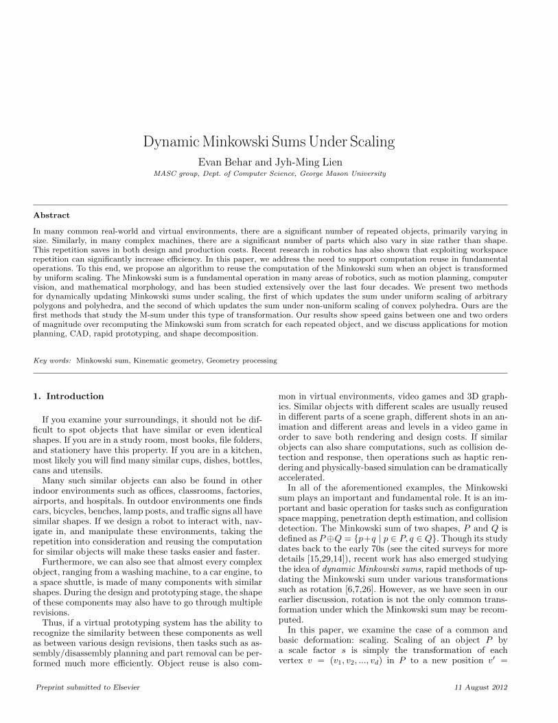
(a) input (b) s = 1 (c) s = 2 (d) convolution s = 1 (e) convolution s = 2

Fig. 1. Comparison of the Minkowski sums [(b) and (c)], and the reduced convolutions [(d) and (e)] for neuron & disc at scales s = 1 ands = 2. The neuron polygon shown in (a) has 18 holes and 1,815 vertices and the disc is represented as a polygon with 32 vertices. Thetopology of the Minkowski sum changes between scales. The definition of the reduced convolution is in Section 3.

(s1v1, s2v2, ..., sdvd), where for v ∈ Rd and si ∈ (0,∞).Uniform scaling consists of the special case where s1 =s2 = ... = sd.

Our goal is to develop an algorithm that can efficientlyupdate the Minkowski sum when the objects are scaledwithout recomputing the Minkowski sum from scratch. Themain challenge comes from the fact that the Minkowskisum can change drastically when the underlying objects arescaled. For example, in Fig. 1, when the disc is scaled totwice its original size, not only the geometry but also thetopology of the Minkowski sum changes.

MainContribution. Our main contributions in this pa-per are two exact, output-sensitive algorithms whose com-putation time depends on the amount of scale and there-fore depends on the number of changes to the Minkowskisum due to scaling.

We base our first method on the Minkowski sum meth-ods in our previous work [8,23], which computes a reducedconvolution of the two polygons or two polyhedra (see defi-nition in Section 3). In 2D, the reduced convolution is a sub-set of the full convolution which omits contributions fromthe reflex vertices of the input polygons. Reflex vertices arevertices whose interior angles are greater than 180 degrees.Two reduced convolutions are illustrated in Fig. 1.

Given this reduced convolution, denoted by P ⊗Q, weshow that there is an efficient way to update both 2DMinkowski sums under scaling regardless of the convex-ity of the input models (Section 4). The set of intersectingfaces in the Minkowski sum changes only at a finite set ofscale values. We call these values critical events, and it ison this notion that our idea rests. As shown in our experi-ments (Section 7), this method is generally one to two or-ders of magnitude faster than recomputing the Minkowskisum from scratch.

We show that this method can be extended naturally to3D (in Section 5). However, we also show that it is not prac-tical to do so due to time and space complexity constraintsas the convolution in 3D is much more complex. To addressthis, in Section 6, we introduce the second method, whichdynamically identifies compatibility errors in the convolu-tion for convex polyhedra and corrects these errors with-out precomputing when they will occur. We show that thismethod supports non-uniform scaling, provides significantspeed improvements over brute force, and does not en-

counter the complexity constraints of precomputation.In addition to reusing computations for the obvious pur-

pose of increasing the computation efficiency, in Section 8we also demonstrate that our method can be extended toanswer the query, “Given the specification of manufactur-ing tolerance, what are the largest and smallest scales ofP for which a given path is valid?” This query is useful inrapid prototyping, for determining the necessary scale forparts to fit into an assembly. With this information we cancheck whether there exists a scale for a part P that canguarantee it fits into the assembly properly. The proposedmethod also finds unusual applications in shape decompo-sition, where it can be used to identify structural featuresbased on multi-scale convolutions.

To the best of our knowledge, this paper presents thefirst work which considers dynamic Minkowski sums underscale and our results are encouraging. However, there aretwo main limitations for the first method. First, it is onlyable to handle uniform scaling, as it relies on the idea thatthe facet normals do not change under scaling. Secondly, itis impractical in more than two dimensions due to its largetime and space complexities. In three or more dimensions,we quickly run up against the curse of dimensionality. Themain limitation of the second method is its inability tohandle non-convex inputs, since it relies on the principlethat each facet in the convolution will be associated withat most one vertex in the input models.

2. Related work

For methods computing static Minkowski sum, detailedsurveys can be found in [15,29,14,5]. A brief discussion ofsome recent works can also be found in Section 3.

Currently there exist few works in computing Minkowskisums for geometric objects under rotation. Many earlyworks can be found in configuration-space (C-space)mapping [24,31,20,28]. These methods generate slices ofC-space obstacles (C-obst) at fixed rotational resolutionusing the Minkowski sums and ignore the temporal andspatial coherence between slices. To avoid this problem,the methods proposed by Avnaim et al. [2] and Brost [9]focus on the idea of contact surfaces, which have a closerelationship to convolution (defined in Section 3). For non-convex polygons, part of the contact region may belong to

2

the interior of the C-obst. Therefore, all contact regionsare tested for intersections and are trimmed around theboundary created by the intersections. Even for simpleshapes many contact regions are trimmed. As a result,significant computation is wasted. In our recent work [6],we address this issue (1) by reducing the number of con-tact regions and (2) by explicitly determining the valuesof rotation θ for which the structure of the Minkowski sumchanges. Our method then computes C-obst by smoothlysweeping the segments of the Minkowski sums betweenconsecutive critical rotations.

However, these methods are limited to 2D polygons andattempts to extend contact surfaces to higher dimensionalspace are still strictly theoretical. [10]. Recently, Mayer etal. [26] have studied transformation of the Minkowski sumunder rotation using the idea of a criticality map, whichstores the rotation values at which the combinatorial struc-ture of the Minkowski sum changes.

Obtaining the full representation of the combinatorialstructure the Minkowski sums of 3D polyhedra under rota-tion is expensive. In many cases, such as penetration depthestimation, it is also unnecessary. In our recent work [22,7],we observe that significant performance gains can be ob-tained if the Minkowski sum is dynamically updated byidentifying and correcting the errors under the given rota-tion. When the input polyhedra are convex, we use the ob-servation that there are only O(n) of certain types of facetsin the sum, where n is the size of input polyhedra, and thatall of the remaining erroneous facets can be identified byfirst locating a linear subset of facets and then performinggradient descent.

3. Preliminaries

In order to provide sufficient background for the read-ers, we briefly discuss the suitability of existing staticMinkowski sum methods for dynamic Minkowski sumsunder scaling.

Many earlier methods based on convex decompositioncompute the pairwise Minkowski sums of the components,and then merge all of the pairwise Minkowski sums. Al-though the main idea of this approach (first proposed byLozano-Perez [24]) is simple, the decomposition and theunion steps can be very tricky and have become the mainfocus of several recent works [1,13,18,29,21].

An additional trouble for the application at hand is thatwhen P is scaled, updating the Minkowski sum using a con-vex decomposition means that once all pairwise Minkowskisums are updated, their union must then be recomputed.This presents a significant hurdle to creating dynamicMinkowski sums using the convex decomposition method.

Due to this, convolution-based approaches becomes moreappealing. The convolution of two shapes P andQ, denotedas P ⊗Q, is a structure produced by combining primitivesfrom the two shapes [16,17]. It is known that the convolu-tion is a superset of the Minkowski sum, that is, P ⊕Q ⊆P ⊗ Q. More specifically, it is known that ∂(P ⊕Q) =∂(P ⊗Q).

The main challenge of the convolution-based meth-ods is in trimming edges and facets in the interior of

p0

p1p2

p3

q0

q1

q2q3

q4

(a) P (left),Q (right)

x

y

(b) P ⊗Q (c) P ⊗Q

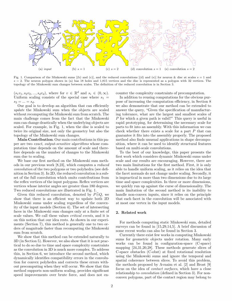
Fig. 2. Polygons P and Q, their convolution P ⊗ Q and reduced

convolution P ⊗Q. In the figure showing P ⊗ Q, x = p0 + q0 andy = p1 + q0. Edge p0p1 is compatible with q0, because p0p1 is onthe counterclockwise turn between q4q0 and q0q1.

the convolution to obtain the Minkowski sum boundary[15,19,30,3,4,27]. For example, Wein [30] computes thearrangement induced by the convolution and keeps thecells with non-zero winding numbers. The arrangement isa data structure representing the subdivision of the spacecreated by the convolution [11]. The winding number ofthe convolution of a point p is the number of times thatconvolution travels counterclockwise around p.

As it will become clear later, convolution methods aremore suitable for dynamically updating Minkowski sumsbecause the combinatorial structure of the convolution typ-ically remains the same when the change to the input modelis small. Additionally, the relationship between the convo-lution edges can be updated in a straightforward way whenthe input models are transformed smoothly.

In the case of uniform scaling, the structure of the con-volution never changes and the structure of the arrange-ment only changes at fixed scale factors, so-called criti-cal scales. This property enables intermediate forms to beupdated rapidly. Additionally, there are far fewer primi-tives in the convolution of two shapes than there are pair-wise Minkowski sums from their decompositions, so the to-tal number of update operations required to reconcile thechange is less.Convolution and Reduced Convolution. The first

method proposed in this paper identifies critical scale fac-tors for each edge in the convolution and updates the ar-rangement of the convolution according to the critical scalefactors. The second method proposed in the paper per-forms dynamic updates on the convolution without com-puting critical events. Our methods can be used in anyconvolution-based method, such as [30,3,4]. However, toease our discussion, we will introduce our method based onthe reduced convolution approach presented in our previ-ous work [23,8], which we review briefly here. In order tocompute the convolution of two shapes, P and Q, we con-sider an edge e of P and a vertex vi of Q. We say that e iscompatible with vi if the direction of e’s outward normalis “between” the directions of the outward normals of vi’sincident facets.

In 2D, we assume P and Q are both counter-clockwiseoriented polygons. Then an edge e and a vertex v are com-patible if the direction of e’s outward normal is betweenthose of v’s incident edges. Note that, this is equivalent tosay that if the direction of e is on the counter-clockwiseturn from (vi−1, vi) to (vi, vi+1). See Fig. 2 for an examplein 2D.

In 3D, f and vi are compatible if the outward normalof f is within the region of the Gaussian map enclosedby the outward normals of vi’s incident facets. Briefly, the

3

Gaussian map is a mapping of a 3D surface to a unit sphere.In the case of polyhedral models, each face is mapped to apoint on the sphere’s surface equal to its unit normal. Thesemapped points are connected by edges if their associatedfaces on the model are adjacent–this maps the edges ofthe model to edges in the Gaussian map. Finally, thesepoint/edge mappings create regions on the surface of thesphere which are the mappings of the vertices on the surfaceof the model.

If f and vi are compatible, then the facet f + v (calledfv-facet) appears in the convolution. Faces of the convolu-tion in 3D may also be formed by an edge from P and anedge from Q (called ee-facet). In this case, the edges arecompatible if their associated edges in the Gaussian mapintersect, in which case the facet eP ⊕ eQ appears in theconvolution.

In order to compute the reduced convolution (RC), wecompute only a subset of the convolution. We exclude con-tributions from reflex vertices (2D) and edges (3D). It hasbeen proven that contributions from reflex vertices andedges are guaranteed to be interior to the Minkowski sum[8]. To extract the Minkowski sum from the reduced con-volution, intersections between the edges and facets of thereduced convolution are computed. Then properly nestedorientable loops (2D) and shells (3D) are extracted fromthe intersections of the RC. Finally, a collision detectionstep is used to detect any remaining errant loops and shells.The worst-case complexity of both algorithms is O(mdnd),for P,Q ⊂ Rd, |P | = m, |Q| = n, which is optimal with re-spect to the worst-case complexity of the Minkowski sumboundary. However, experimentally, our method is shownto be much faster than Wein’s [30].

4. Uniform Scaling in 2D

We seek to update the Minkowski sum of polygons P andQ transforming under uniform scales. We assume withoutloss of generality that P scales uniformly and Q remainsfixed. Since the Minkowski sum is commutative, scaling Qcan be done identically by simply swapping P and Q inthe input order. The uniform scaling operation P ′ = sPgenerates P ′ such that for every point v ∈ P , sv ∈ P ′. Akey observation is that when P scales by s, the outwardnormals of all its line segments remain the same, and soscaling of P does not change the combinatorial structure ofthe reduced convolution (RC); only the length and positionof the segments in RC change.

Even though the combinatorial structure of the RC doesnot change when P is scaled, the outer boundary of theMinkowski sum will change. In particular, the set of edges(2D) or facets (3D) which intersect with each other maychange–some intersections may be deleted while others maybe added. We call these additions and deletions criticalevents.

To use these critical events, we compute the ranges ofs within which intersections between edges actually occur.We can then add or delete intersections by stepping throughthe critical events between two values of s. When we fin-ish adding and deleting intersections in this way, we cancorrectly and efficiently update by considering only those

∆xI(s)

xI1

xI0

svpsvp

(a) T-edge

∆xI(s)

xI1

xI0

sep0sep1

(b) S-edge

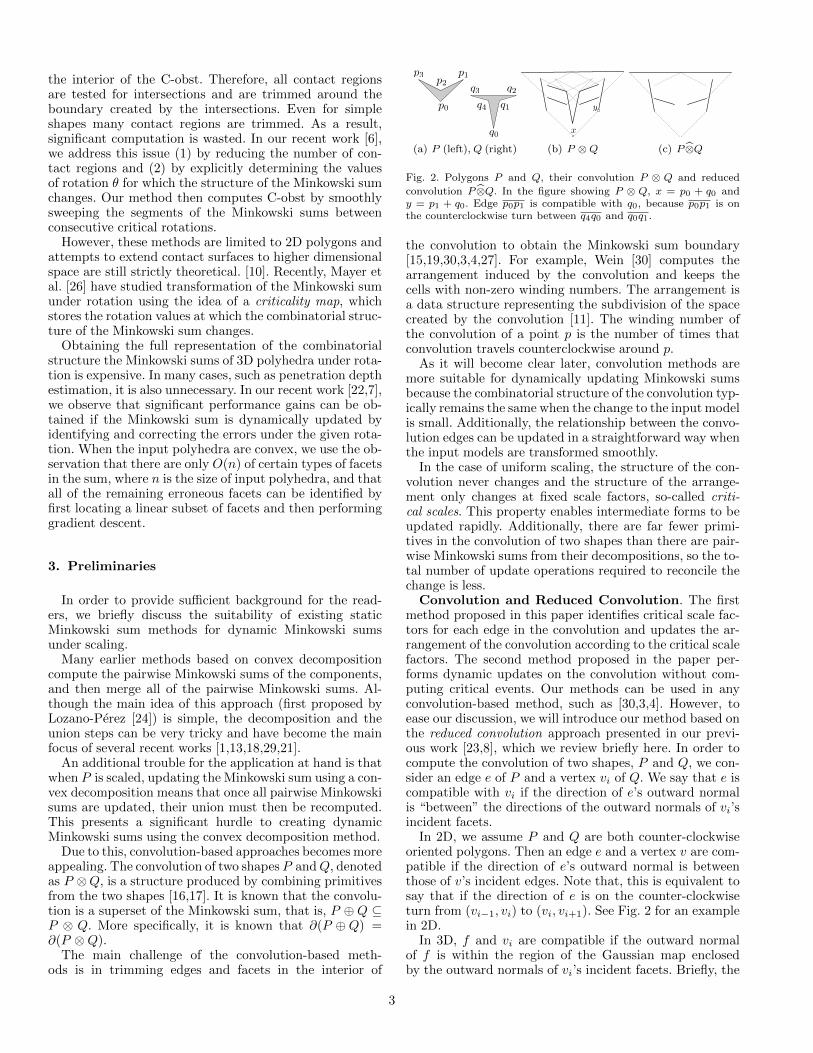
Fig. 3. In (a) an edge from Q and a vertex from P form a T-edgein the convolution, so the segment only translates as s changes. In(b) an edge from P and a vertex from Q form an S-edge edge, sothe segment also scales as it translates. In both cases the underlyinglines translate.

intersections between line segments that are valid for thegiven s.

4.1. Tracking the intersection values in 2D

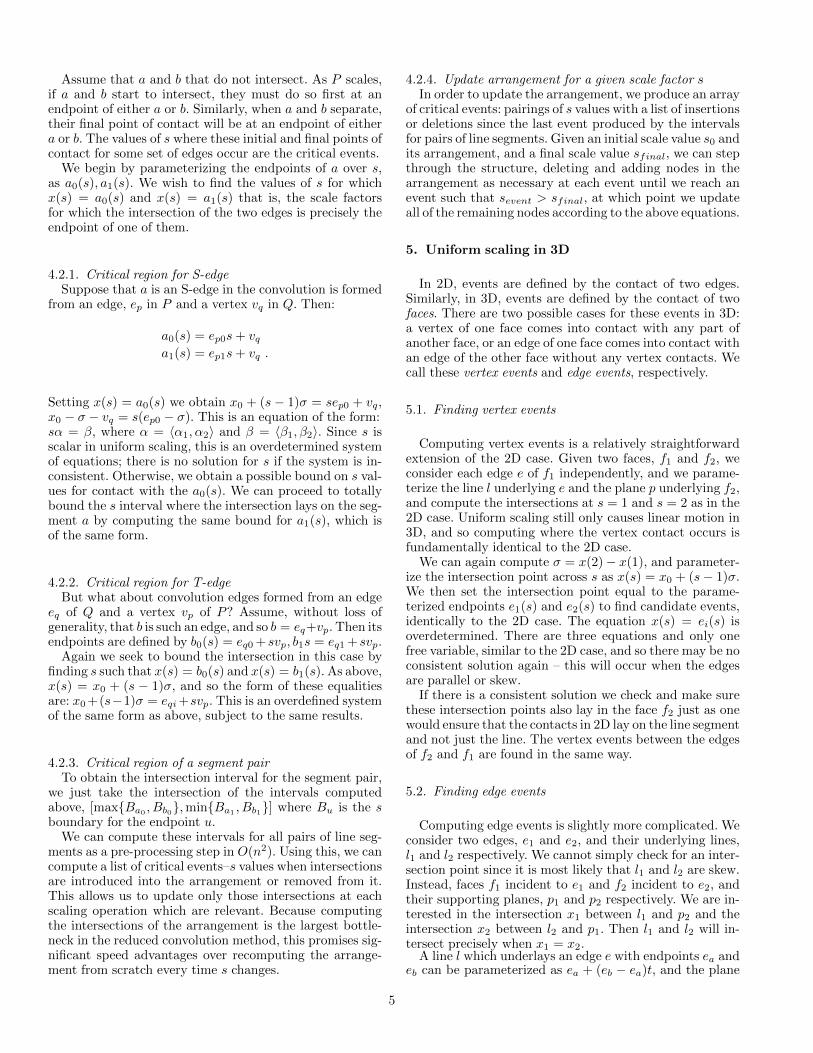
Consider a single edge of the convolution, a. Suppose ais formed from the contribution of an edge of P , ep, and avertex of Q, vq. Then a = ep + vq, that is, ep translatedby vq. When P scales, only ep changes, so a(s) = sep + vq.Because such edges are scaled as P is scaled, we call themS-edges. Note that S-edges will also be translated in theupdated convolution. Similarly, if a is formed from an edgeof Q, eq and a vertex of P , vp, then a = eq +vp, and a(s) =eq + svp, since only P scales. We call such edges T-edgesince as P is scaled, they are translated but not scaled.Fig. 3 illustrates both types of edges.

Now consider two line segments a and b in the convo-lution, and let their endpoints be (a0, a1) and (b0, b1), re-spectively. Let the underlying lines of a and b be la and lb,respectively. We parameterize the intersection point of laand lb over s ∈ (0,∞). To do this, we consider the param-eterized forms of la and lb:

la(r) = a0 + r(a1 − a0) = a0 + rv

lb(t) = b0 + t(b1 − b0) = b0 + tw ,

where v = a1 − a0 and w = b1 − b0.Observation 1 Let u = a0 − b0. Then the intersectionpoint of la and lb is at

rI =vyux − vxux

vxwy − vywx,

and the coordinate of that intersection is xa(rI) = a0 +rIv.The parameterized form lets us find the critical events

we are looking for.

4.2. Finding critical regions

Let x(s) be the intersection point between the line lacontaining a and the line lb containing b when P is scaledby a factor of s. x(s) is a parameterized line as well. Letthe intersection point computed above be x0. This intersec-tion is computed at the base scale value, s = 1. Therefore,x(1) = x0. Then we can define x(s) = x0 + (s − 1)σ for aslope vector σ. It is easy to recompute the line segments atsome other scale, s′, and compute the intersection of the

new lines to find x(s′) = x0+(s′−1)σ, and so σ = x(s′)−x0

s′−1 .

We choose s′ = 2, since in this case, s′ − 1 = 1 and soσ = x(2)− x(1), which eliminates the division.

4

Assume that a and b that do not intersect. As P scales,if a and b start to intersect, they must do so first at anendpoint of either a or b. Similarly, when a and b separate,their final point of contact will be at an endpoint of eithera or b. The values of s where these initial and final points ofcontact for some set of edges occur are the critical events.

We begin by parameterizing the endpoints of a over s,as a0(s), a1(s). We wish to find the values of s for whichx(s) = a0(s) and x(s) = a1(s) that is, the scale factorsfor which the intersection of the two edges is precisely theendpoint of one of them.

4.2.1. Critical region for S-edgeSuppose that a is an S-edge in the convolution is formed

from an edge, ep in P and a vertex vq in Q. Then:

a0(s) = ep0s+ vqa1(s) = ep1s+ vq .

Setting x(s) = a0(s) we obtain x0 + (s− 1)σ = sep0 + vq,x0 − σ − vq = s(ep0 − σ). This is an equation of the form:sα = β, where α = 〈α1, α2〉 and β = 〈β1, β2〉. Since s isscalar in uniform scaling, this is an overdetermined systemof equations; there is no solution for s if the system is in-consistent. Otherwise, we obtain a possible bound on s val-ues for contact with the a0(s). We can proceed to totallybound the s interval where the intersection lays on the seg-ment a by computing the same bound for a1(s), which isof the same form.

4.2.2. Critical region for T-edgeBut what about convolution edges formed from an edge

eq of Q and a vertex vp of P? Assume, without loss ofgenerality, that b is such an edge, and so b = eq+vp. Then itsendpoints are defined by b0(s) = eq0 + svp, b1s = eq1 + svp.

Again we seek to bound the intersection in this case byfinding s such that x(s) = b0(s) and x(s) = b1(s). As above,x(s) = x0 + (s − 1)σ, and so the form of these equalitiesare: x0 +(s−1)σ = eqi +svp. This is an overdefined systemof the same form as above, subject to the same results.

4.2.3. Critical region of a segment pairTo obtain the intersection interval for the segment pair,

we just take the intersection of the intervals computedabove, [max{Ba0 , Bb0},min{Ba1 , Bb1}] where Bu is the sboundary for the endpoint u.

We can compute these intervals for all pairs of line seg-ments as a pre-processing step in O(n2). Using this, we cancompute a list of critical events–s values when intersectionsare introduced into the arrangement or removed from it.This allows us to update only those intersections at eachscaling operation which are relevant. Because computingthe intersections of the arrangement is the largest bottle-neck in the reduced convolution method, this promises sig-nificant speed advantages over recomputing the arrange-ment from scratch every time s changes.

4.2.4. Update arrangement for a given scale factor sIn order to update the arrangement, we produce an array

of critical events: pairings of s values with a list of insertionsor deletions since the last event produced by the intervalsfor pairs of line segments. Given an initial scale value s0 andits arrangement, and a final scale value sfinal, we can stepthrough the structure, deleting and adding nodes in thearrangement as necessary at each event until we reach anevent such that sevent > sfinal, at which point we updateall of the remaining nodes according to the above equations.

5. Uniform scaling in 3D

In 2D, events are defined by the contact of two edges.Similarly, in 3D, events are defined by the contact of twofaces. There are two possible cases for these events in 3D:a vertex of one face comes into contact with any part ofanother face, or an edge of one face comes into contact withan edge of the other face without any vertex contacts. Wecall these vertex events and edge events, respectively.

5.1. Finding vertex events

Computing vertex events is a relatively straightforwardextension of the 2D case. Given two faces, f1 and f2, weconsider each edge e of f1 independently, and we parame-terize the line l underlying e and the plane p underlying f2,and compute the intersections at s = 1 and s = 2 as in the2D case. Uniform scaling still only causes linear motion in3D, and so computing where the vertex contact occurs isfundamentally identical to the 2D case.

We can again compute σ = x(2)− x(1), and parameter-ize the intersection point across s as x(s) = x0 + (s− 1)σ.We then set the intersection point equal to the parame-terized endpoints e1(s) and e2(s) to find candidate events,identically to the 2D case. The equation x(s) = ei(s) isoverdetermined. There are three equations and only onefree variable, similar to the 2D case, and so there may be noconsistent solution again – this will occur when the edgesare parallel or skew.

If there is a consistent solution we check and make surethese intersection points also lay in the face f2 just as onewould ensure that the contacts in 2D lay on the line segmentand not just the line. The vertex events between the edgesof f2 and f1 are found in the same way.

5.2. Finding edge events

Computing edge events is slightly more complicated. Weconsider two edges, e1 and e2, and their underlying lines,l1 and l2 respectively. We cannot simply check for an inter-section point since it is most likely that l1 and l2 are skew.Instead, faces f1 incident to e1 and f2 incident to e2, andtheir supporting planes, p1 and p2 respectively. We are in-terested in the intersection x1 between l1 and p2 and theintersection x2 between l2 and p1. Then l1 and l2 will in-tersect precisely when x1 = x2.

A line l which underlays an edge e with endpoints ea andeb can be parameterized as ea + (eb − ea)t, and the plane

5

p which underlies triangle t with vertices ta, tb, tc can beparameterized as ta + (tb − ta)u+ (tc − ta)v. We set theseequal to each other and simplify, yielding

ea − ta =

ea − eb

tb − ta

tc − ta

T t

u

v

.

We have five vertices from the convolution in this equa-tion, ea, eb, ta, tb, tc, each of which is parameterized in thescale domain by its P and Q components, v = vq + svp.Substituting, we obtain expressions for t, u and v parame-terized by s: t

u

v

=

eaq − ebq + s(eap − ebp)

tbq − taq + s(tbp − tap)

tcq − taq + s(tcp − tap)

T−1

(eaq−taq+s(eap−tap)) .

c1

c6

c5

c4

c3

c2

Fig. 4. Degenerateee contacts for paral-lel faces, contacts aremarked as c1 throughc6. Notice that novertices are involvedin this event.

When we solve this for l1 and p2as well as l2 and p1, we obtain twoexpressions in s for the intersectionsof the line and the plane, which wecan set equal to each other and solvefor s.Parallel faces When f1 and f2

are parallel but not always coplanar,then ea − eb

tb − ta

tc − ta

T

,

will be singular, and so we will notbe able to detect edge events in the usual way. If any vertexof either face is involved in the contact, then we will cor-rectly detect these events as vertex events, but it is possiblethat this isn’t the case. Figure 4 shows a situation in whichtwo coplanar faces have no vertex contacts. In order to de-termine whether an event will occur, we must find the scalevalue when the faces are coplanar, and then check the edgesof the faces for intersections at that scale. Fortunately, thedetection for vertex events is robust enough that it doesnot need to deal with parallel faces as a special case.

To determine the value of s where the faces are coplanar,we pick an arbitrary vertex v on f1 and proceed as thoughwe were detecting a vertex event with f2. However, we donot need to check if v(sevent) is inside of f2, since we areonly interested in the value of s where v hits p2–this willbe the value of s at which the faces are coplanar.

Because of this, we do not need to perform the usual edgeevent detection at all when dealing with parallel faces. Forthese faces, we find the scale of contact from the vertexevent detection step. If there are no vertex events, we checkfor edge intersections to see if there are any edge events.

Coplanar faces Finally, in some cases, f1 and f2 willalways be coplanar. In these coplanar cases, the contactpossibilities for f1 and f2 reduce to the 2D case, in whichedge events are impossible. Therefore, we can use the logicfrom the 2D scaling directly in order to detect the eventsfor the coplanar faces by transforming f1 and f2 into thexy-plane, and applying 2D vertex event detection.

6. Non-uniform scaling for convex polyhedra

In three dimensions, the worst-case complexity of theevent space is O(m4n4). The memory necessary to storethe event structure and the time necessary to compute itrapidly become overwhelming. While there are several prac-tical strategies for mitigating memory issues, including nar-rowing the scaling domain to a smaller window and diskswapping, the event space must be computed for all pairsof faces, resulting in worst-case time complexity. Enumer-ating all critical events also makes the extension to non-uniform scaling almost impossible. As a result, we look toa method with less pre-computation.

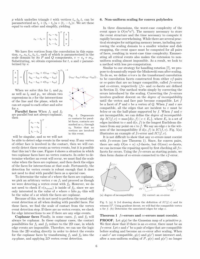
Similar to our strategy for handling rotation [7], we pro-pose to dynamically repair the Minkowski sum after scaling.To do so, we define errors in the transformed convolutionto be convolution facets constructed from either vf -pairsor ee-pairs that are no longer compatible, called fv-errorsand ee-errors, respectively (fv- and ee-facets are definedin Section 3). Our method works simply by correcting theerrors introduced by the scaling. Correcting the fv-errorsinvolves gradient descent on the degree of incompatibilityuntil the vertex and face pair become compatible. Let fbe a facet of P and v be a vertex of Q. When f and v arecompatible, all the edges that are incident to v must bebelow or on the half-plane supported by f . When f and vare incompatible, we can define the degree of incompatibil-ity: IC(f, v) = max{d(e, f) | e ∈ Ev}, where Ev is a set ofedges incident to v and d(e, f) is the longest Euclidean dis-tance from any point on e to f . We say an edge e is the wit-ness of the incompatibility if d(e, f) is IC(f, v). Fig. 5(a)illustrates an example of fv-error and IC(f, v).

It is not difficult to show that any ee-errors must coexistwith fv-errors (see Theorem 1). Since, for convex pairs,there are only O(m + n) vf -facets, but O(mn) ee-facets,we can increase the repairing speed by first checking all fv-facets for errors. Using the fv-errors as starting points, wethen form chains of ee-errors connected to the vf -error.

nf

f

v

IC(f, v)

v�

u

(a) degree of incompatibility

e

f−

f+ q+

q−

g(q−)g(q+)

g(f+)g(f−)g(e)

(b) correct an ee-error

Fig. 5. (a) A 2-d drawing shows the definition of IC(f, v) and its

witness vv′. Using gradient decent, we will find the compatible vertexu for f . (b) Determine the associated edges for edge e.

Theorem 1 fv-errors and ee-errors must coexist.

PROOF. Let g(p) be the Gaussian map of a primitive p.We first show that if there is an ee-error, there must be anfv-error. Let e and e′ be a pair of edges that are compatiblebefore scaling and become an ee-error after scaling. Whene and e′ are compatible, g(e) and g(e′) must intersect and,after a non-uniform scaling of P , g(e) and g(e′) no longer

6

intersect. This means at a certain point during the scaling,an end point of g(e) must cross g(e′) or vice versa. When apoint v crosses the edge g(e), v changes the face with whichit is associated from one side of g(e) to the other side ofg(e). This change indicates that there must be an fv-error.

We then show that if there is an fv-error, there must bean ee-error. If a facet f of P and a vertex v of Q becomean fv-error, we know that f now must be compatible withsome other vertex v′ 6= v of Q. As a result, an edge g(e)incident to g(f) must be moved (or deformed) with g(f).Since the faces in g(Q) are convex and g(e) cannot intersectwith a segment more than twice, g(e) must intersect withsome new edges of Q when g(f) moves from g(v) to g(v′).This indicates that there must be at least one ee-error.

Therefore, fv-errors and ee-errors must coexist. 2

More specifically, let e be such an edge from P involvedin an ee-error, and let f− and f+ be the facets in P incidentto e. Assume that the facets f− and f+ both have the com-patible vertices q− and q+ of Q. If we overlay the Gaussianmap g(e) of e with g(Q), g(e) will intersect a set of faces ing(Q) and the end points of g(e) are inside g(q−) and g(q+).See the bottom of Fig. 5(b). If we can determine the restof the faces intersected by g(e), we can find the compatibleedges for e. We further know that these faces form a con-nected component between g(q−) and g(q+), thus the com-patible edges for e must be on the boundary of these faces.To find these Gaussian faces, we start from g(q−), and findan incident edge e′ of g(q−) that is compatible with e.

Because both P and Q are convex, the faces f1 and f2incident to e will each be compatible with precisely onevertex, v1 and v2 respectively. The edges with which e iscompatible must form a path from v1 to v2 along the surfaceof the model. We check each of v1’s incident edges to find theedge with which e is compatible. We then replace v1 withthe vertex at the other end-point of the compatible edge,and repeat, ignoring the incident edge which has alreadybeen found to be compatible. When we find v2 by this path,we have enumerated all of the compatible vertices. Thecomplexity of this update is O(|E|), where E is the set ofedges incident to at least one vertex in the path.

In convex pairs, each face of P will be paired with pre-cisely one vertex of Q and vice-versa. We depend on thisrelationship in order to correctly identify errors. An exten-sion to non-convex inputs depends on the existence of aconvex map–a convex polyhedron whose Gaussian map isidentical to the arrangement of the Gaussian map of thenon-convex input. Discussion of the convex map is outsidethe scope of this paper.

7. Results

Our implementations are based on the publicly avail-able implementation from our previous work in 2D [8] and3D [7]. All experiments reported in this section are per-formed on a machine with Intel CPUs at 2.13 GHz with 4GB RAM and our implementation is coded in C++, usingGNU MPFR and the MPFRC++ wrapper for high preci-sion arithmetic.

(a) G1 (30) (b) G2 (34) (c)G3(24)

(d) G4 (43) (e) dog (145)

Fig. 6. Models used in the experiments. The figure shows the namesand the sizes of the polygons. Note that (c) is G3 (24).

7.1. Results from uniform Scaling in 2D

Table 1Average speed-up of the 2D enumerative dynamic update algorithmover 100 random re-scalings. Models in the first column are the modelbeing scaled in each experiment, while models in the first row arethe static (unscaled) model. The bolded figures are the lowest andhighest speed-up values achieved.

dog g1 g2 g3 g4

dog 28.911 115.651 5.592 32.408 6.538

g1 115.651 131.150 432.069 533.141 473.282

g2 15.223 313.710 298.038 161.712 88.916

g3 112.354 152.790 171.825 34.347 79.362

g4 14.519 201.861 45.220 80.230 122.565

Table 1 shows average speed-up factors for several modelpairs in Fig. 6 across the scaling domain [0.1, 10] in incre-ments of 0.1 scale factor. Speed-up is computed as tstatic

tdynamic

over 100 random re-scalings. Our method is always fasterthan recomputing from scratch and is on average 150.682times faster. The largest speedup is over two orders of mag-nitude (from g1 ⊕ g4) and even on model pairs with highevent density (dog ⊕ g2 in Table 1), the proposed methodis faster though the improvement here is more marginal.

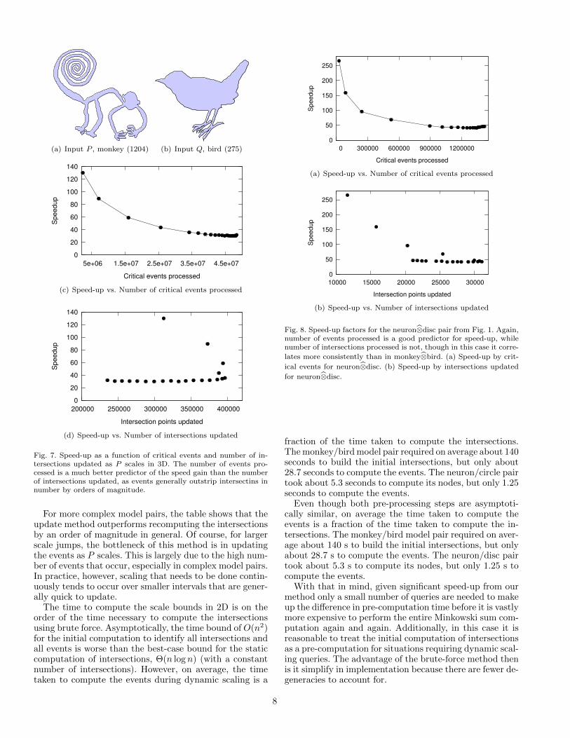
The results in Fig. 7 show speed-up factors on one of themore complex model pairs, shown in Figs. 7(a) and 7(b).The monkey model contains 1204 vertices, and the birdmodel has 275 vertices. Their reduced convolution contains16,425 segments. When the monkey is scaled along the in-terval s ∈ (0,∞], there are 56,996,430 critical events.

Fig. 8 shows speed-up factors for the neuron⊗disc pairshown in Fig. 1. There are 1815 vertices in the neuron modeland 32 vertices in the disc model. The reduced convolu-tion of the neuron and the disc has 3196 segments. Thereare 56238 critical events discovered when the disc is scaledacross s ∈ (0,∞).

7

(a) Input P , monkey (1204) (b) Input Q, bird (275)

0

20

40

60

80

100

120

140

5e+06 1.5e+07 2.5e+07 3.5e+07 4.5e+07

Spe

edup

Critical events processed

(c) Speed-up vs. Number of critical events processed

0

20

40

60

80

100

120

140

200000 250000 300000 350000 400000

Spe

edup

Intersection points updated

(d) Speed-up vs. Number of intersections updated

Fig. 7. Speed-up as a function of critical events and number of in-tersections updated as P scales in 3D. The number of events pro-cessed is a much better predictor of the speed gain than the numberof intersections updated, as events generally outstrip intersectins innumber by orders of magnitude.

For more complex model pairs, the table shows that theupdate method outperforms recomputing the intersectionsby an order of magnitude in general. Of course, for largerscale jumps, the bottleneck of this method is in updatingthe events as P scales. This is largely due to the high num-ber of events that occur, especially in complex model pairs.In practice, however, scaling that needs to be done contin-uously tends to occur over smaller intervals that are gener-ally quick to update.

The time to compute the scale bounds in 2D is on theorder of the time necessary to compute the intersectionsusing brute force. Asymptotically, the time bound of O(n2)for the initial computation to identify all intersections andall events is worse than the best-case bound for the staticcomputation of intersections, Θ(n log n) (with a constantnumber of intersections). However, on average, the timetaken to compute the events during dynamic scaling is a

0

50

100

150

200

250

0 300000 600000 900000 1200000

Spe

edup

Critical events processed

(a) Speed-up vs. Number of critical events processed

0

50

100

150

200

250

10000 15000 20000 25000 30000

Spe

edup

Intersection points updated

(b) Speed-up vs. Number of intersections updated

Fig. 8. Speed-up factors for the neuron⊗disc pair from Fig. 1. Again,number of events processed is a good predictor for speed-up, whilenumber of intersections processed is not, though in this case it corre-

lates more consistently than in monkey⊗bird. (a) Speed-up by crit-

ical events for neuron⊗disc. (b) Speed-up by intersections updated

for neuron⊗disc.

fraction of the time taken to compute the intersections.The monkey/bird model pair required on average about 140seconds to build the initial intersections, but only about28.7 seconds to compute the events. The neuron/circle pairtook about 5.3 seconds to compute its nodes, but only 1.25seconds to compute the events.

Even though both pre-processing steps are asymptoti-cally similar, on average the time taken to compute theevents is a fraction of the time taken to compute the in-tersections. The monkey/bird model pair required on aver-age about 140 s to build the initial intersections, but onlyabout 28.7 s to compute the events. The neuron/disc pairtook about 5.3 s to compute its nodes, but only 1.25 s tocompute the events.

With that in mind, given significant speed-up from ourmethod only a small number of queries are needed to makeup the difference in pre-computation time before it is vastlymore expensive to perform the entire Minkowski sum com-putation again and again. Additionally, in this case it isreasonable to treat the initial computation of intersectionsas a pre-computation for situations requiring dynamic scal-ing queries. The advantage of the brute-force method thenis it simplify in implementation because there are fewer de-generacies to account for.

8

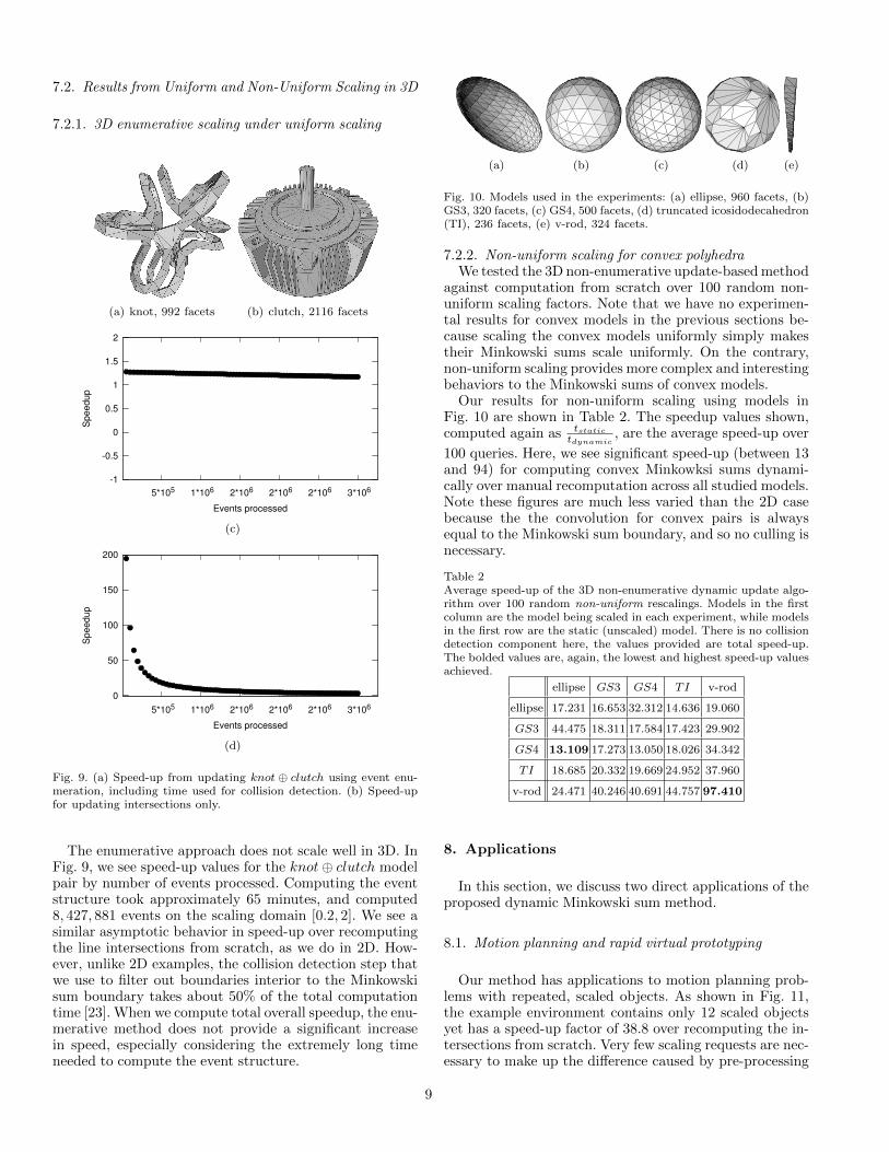
7.2. Results from Uniform and Non-Uniform Scaling in 3D

7.2.1. 3D enumerative scaling under uniform scaling

(a) knot, 992 facets (b) clutch, 2116 facets

-1

-0.5

0

0.5

1

1.5

2

5*105 1*106 2*106 2*106 2*106 3*106

Spe

edup

Events processed

(c)

0

50

100

150

200

5*105 1*106 2*106 2*106 2*106 3*106

Spe

edup

Events processed

(d)

Fig. 9. (a) Speed-up from updating knot ⊕ clutch using event enu-meration, including time used for collision detection. (b) Speed-upfor updating intersections only.

The enumerative approach does not scale well in 3D. InFig. 9, we see speed-up values for the knot⊕ clutch modelpair by number of events processed. Computing the eventstructure took approximately 65 minutes, and computed8, 427, 881 events on the scaling domain [0.2, 2]. We see asimilar asymptotic behavior in speed-up over recomputingthe line intersections from scratch, as we do in 2D. How-ever, unlike 2D examples, the collision detection step thatwe use to filter out boundaries interior to the Minkowskisum boundary takes about 50% of the total computationtime [23]. When we compute total overall speedup, the enu-merative method does not provide a significant increasein speed, especially considering the extremely long timeneeded to compute the event structure.

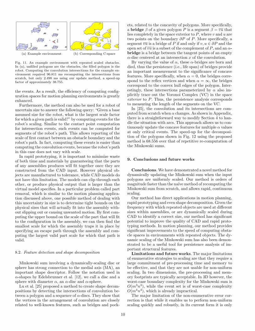
(a) (b) (c) (d) (e)

Fig. 10. Models used in the experiments: (a) ellipse, 960 facets, (b)GS3, 320 facets, (c) GS4, 500 facets, (d) truncated icosidodecahedron(TI), 236 facets, (e) v-rod, 324 facets.

7.2.2. Non-uniform scaling for convex polyhedraWe tested the 3D non-enumerative update-based method

against computation from scratch over 100 random non-uniform scaling factors. Note that we have no experimen-tal results for convex models in the previous sections be-cause scaling the convex models uniformly simply makestheir Minkowski sums scale uniformly. On the contrary,non-uniform scaling provides more complex and interestingbehaviors to the Minkowski sums of convex models.

Our results for non-uniform scaling using models inFig. 10 are shown in Table 2. The speedup values shown,computed again as tstatic

tdynamic, are the average speed-up over

100 queries. Here, we see significant speed-up (between 13and 94) for computing convex Minkowksi sums dynami-cally over manual recomputation across all studied models.Note these figures are much less varied than the 2D casebecause the the convolution for convex pairs is alwaysequal to the Minkowski sum boundary, and so no culling isnecessary.

Table 2Average speed-up of the 3D non-enumerative dynamic update algo-rithm over 100 random non-uniform rescalings. Models in the firstcolumn are the model being scaled in each experiment, while modelsin the first row are the static (unscaled) model. There is no collisiondetection component here, the values provided are total speed-up.The bolded values are, again, the lowest and highest speed-up valuesachieved.

ellipse GS3 GS4 TI v-rod

ellipse 17.231 16.653 32.312 14.636 19.060

GS3 44.475 18.311 17.584 17.423 29.902

GS4 13.109 17.273 13.050 18.026 34.342

TI 18.685 20.332 19.669 24.952 37.960

v-rod 24.471 40.246 40.691 44.757 97.410

8. Applications

In this section, we discuss two direct applications of theproposed dynamic Minkowski sum method.

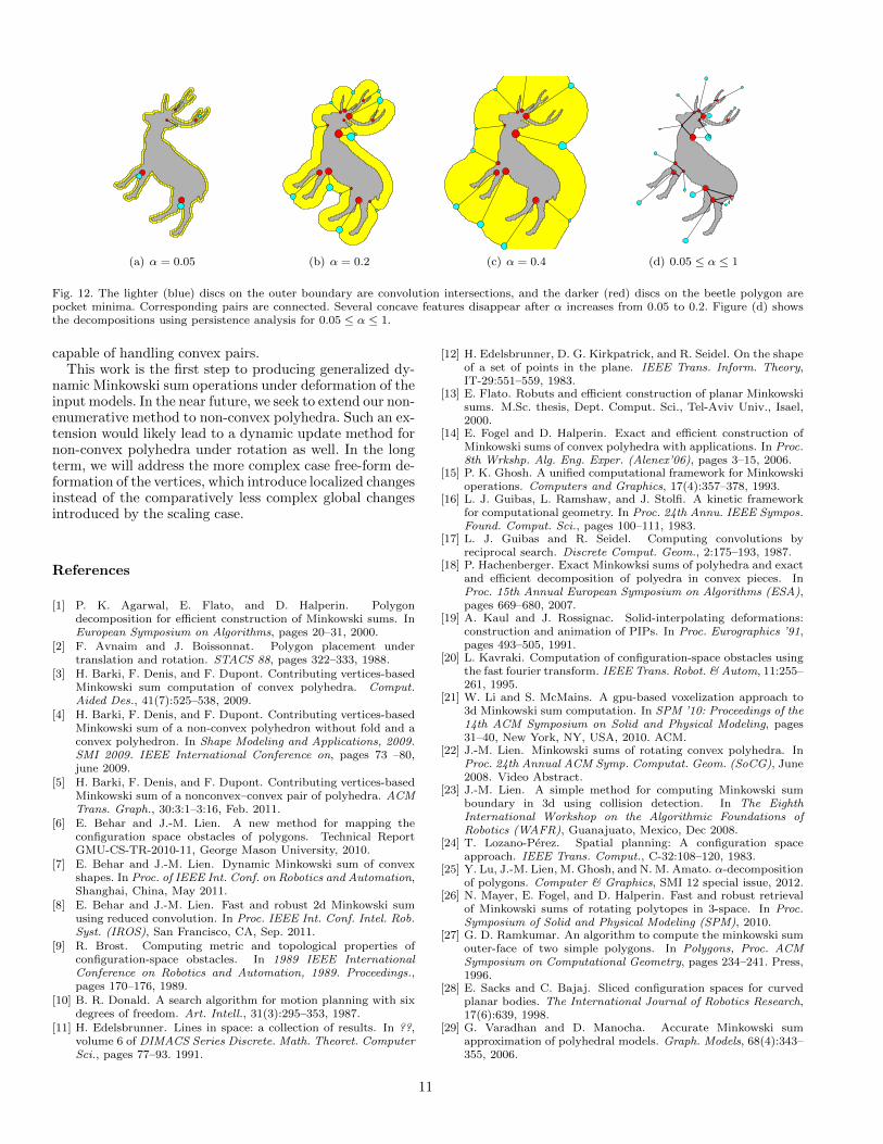
8.1. Motion planning and rapid virtual prototyping

Our method has applications to motion planning prob-lems with repeated, scaled objects. As shown in Fig. 11,the example environment contains only 12 scaled objectsyet has a speed-up factor of 38.8 over recomputing the in-tersections from scratch. Very few scaling requests are nec-essary to make up the difference caused by pre-processing

9

KSEP

WXEVX

(a) Example environment

WXEVX

KSEP

(b) Corresponding C-space

Fig. 11. An example environment with repeated scaled obstacles.In (a), unfilled polygons are the obstacles, the filled polygon is therobot. Computing the convolution intersections for the example en-vironment required 96.811 ms recomputing the intersections fromscratch, but only 2.498 ms using our update method, a speed-upfactor of approximately 38.755.

the events. As a result, the efficiency of computing config-uration spaces for motion planning environments is greatlyenhanced.

Furthermore, the method can also be used for a robot ofuncertain size to answer the following query: “Given a baseassumed size for the robot, what is the largest scale factorfor which a given path is valid?” by computing events for therobot’s scaling. Similar to the contact point computationfor intersection events, such events can be computed forsegments of the robot’s path. This allows reporting of thescale of first contact between an obstacle boundary and therobot’s path. In fact, computing these events is easier thancomputing the convolution events, because the robot’s pathin this case does not vary with scale.

In rapid prototyping, it is important to minimize wasteof both time and materials by guaranteeing that the partsof any assemblies produces will fit together once they areconstructed from the CAD input. However physical ob-jects are manufactured to tolerance, while CAD models donot have this limitation. The models can clip through eachother, or produce physical output that is larger than thevirtual model specifies. In a particular problem called partremoval, which is similar to the motion planning applica-tion discussed above, one possible method of dealing withthis uncertainty in size is to determine tight bounds on thephysical sizes that will actually fit into the assembly with-out slipping out or causing unwanted motion. By first com-puting the upper bound on the scale of the part that will fitto the configuration in the assembly, we can then find thesmallest scale for which the assembly traps it in place byspecifying an escape path through the assembly and com-puting the largest valid part scale for which that path isvalid.

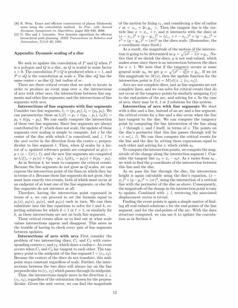
8.2. Feature detection and shape decomposition

Minkowski sum involving a dynamically-scaling disc orsphere has strong connection to the medial axis (MA), animportant shape descriptor. Follow the notation used inα-shapes by Edelsbrunner et al. [12], we call a disc and asphere with diameter α, an α-disc and α-sphere.

Lu et al. [25] proposed a method to create shape decom-positions by detecting the intersections of convolution be-tween a polygon and a sequence of α-discs. They show thatthe vertices in the arrangement of convolution are closelyrelated to well-known features, such as bridges and pock-

ets, related to the concavity of polygons. More specifically,a bridge β of a given polygon P is a segment β = vu thatlies completely in the space exterior to P , where v and u aretwo points on the boundary ∂P of P . More specifically, asegment vu is a bridge of P if and only if v, u ∈ ∂P and theopen set of vu is a subset of the complement of P , and an α-bridge is a bridge between the tangent points of an emptyα-disc centered at an intersection x of the convolution.

By varying the value of α, these α-bridges are born anddied, thus the persistence (i.e., life span) of bridges providean important measurement to the significance of concavefeatures. More specifically, when α = 0, the bridges corre-spond to the reflex vertices and when α = ∞, the bridgescorrespond to the convex hull edges of the polygon. Inter-estingly, these intersections parameterized by α also im-plicitly trace out the Voronoi Complex (VC) in the spaceexterior to P . Thus, the persistence analysis correspondsto measuring the length of the segments on the VC.

In [25], the convolution and its intersections are com-puted from scratch when α changes. As shown in Appendix,there is a straightforward way to modify Section 4 to han-dle the situation with arcs. This approach allows us to con-tinuously update the concave features for multiple α valuesat only critical events. The speed-up for the decomposi-tion of the polygons shown in Fig. 12 using the proposedmethod is 68.556 over that of repetitive re-computation ofthe Minkowski sums.

9. Conclusions and future works

Conclusions. We have demonstrated a novel method fordynamically updating the Minkowski sum when the inputpolygons are uniformly scaled. Our method is orders ofmagnitude faster than the naıve method of recomputing theMinkowski sum from scratch, and allows rapid, continuousscaling.

Our method has direct applications in motion planning,rapid prototyping and even shape decomposition. Given thefrequency with which repeated objects are used at differentsizes within assemblies, or are dynamically scaled duringCAD to identify a correct size, our method has significantpotential to improve the quality of CAD and rapid proto-typing methods. In motion planning, our method providessignificant improvements to the speed of computing obsta-cle spaces in environments with repeated objects. The dy-namic scaling of the Minkowski sum has also been demon-strated to be a useful tool for persistence analysis of im-portant structural features.Limitations and future works. The major limitations

of enumerative strategies to scaling are that they require alarge commitment of pre-processing time and memory tobe effective, and that they are not usable for non-uniformscaling. In two dimensions, the pre-processing and mem-ory footprints are typically acceptable. In 3D however, theworst-case boundary complexity for the Minkowski sum isO(m3n3), while the event set is of worst-case complexityO(m4n4), which is already impractical.

The major limitation of the non-enumerative error cor-rection is that while it enables us to perform non-uniformscaling quickly and robustly, in its current form it is only

10

(a) α = 0.05 (b) α = 0.2 (c) α = 0.4 (d) 0.05 ≤ α ≤ 1

Fig. 12. The lighter (blue) discs on the outer boundary are convolution intersections, and the darker (red) discs on the beetle polygon arepocket minima. Corresponding pairs are connected. Several concave features disappear after α increases from 0.05 to 0.2. Figure (d) showsthe decompositions using persistence analysis for 0.05 ≤ α ≤ 1.

capable of handling convex pairs.This work is the first step to producing generalized dy-

namic Minkowski sum operations under deformation of theinput models. In the near future, we seek to extend our non-enumerative method to non-convex polyhedra. Such an ex-tension would likely lead to a dynamic update method fornon-convex polyhedra under rotation as well. In the longterm, we will address the more complex case free-form de-formation of the vertices, which introduce localized changesinstead of the comparatively less complex global changesintroduced by the scaling case.

References

[1] P. K. Agarwal, E. Flato, and D. Halperin. Polygondecomposition for efficient construction of Minkowski sums. InEuropean Symposium on Algorithms, pages 20–31, 2000.

[2] F. Avnaim and J. Boissonnat. Polygon placement undertranslation and rotation. STACS 88, pages 322–333, 1988.

[3] H. Barki, F. Denis, and F. Dupont. Contributing vertices-basedMinkowski sum computation of convex polyhedra. Comput.Aided Des., 41(7):525–538, 2009.

[4] H. Barki, F. Denis, and F. Dupont. Contributing vertices-basedMinkowski sum of a non-convex polyhedron without fold and aconvex polyhedron. In Shape Modeling and Applications, 2009.SMI 2009. IEEE International Conference on, pages 73 –80,june 2009.

[5] H. Barki, F. Denis, and F. Dupont. Contributing vertices-basedMinkowski sum of a nonconvex–convex pair of polyhedra. ACMTrans. Graph., 30:3:1–3:16, Feb. 2011.

[6] E. Behar and J.-M. Lien. A new method for mapping theconfiguration space obstacles of polygons. Technical ReportGMU-CS-TR-2010-11, George Mason University, 2010.

[7] E. Behar and J.-M. Lien. Dynamic Minkowski sum of convexshapes. In Proc. of IEEE Int. Conf. on Robotics and Automation,Shanghai, China, May 2011.

[8] E. Behar and J.-M. Lien. Fast and robust 2d Minkowski sumusing reduced convolution. In Proc. IEEE Int. Conf. Intel. Rob.Syst. (IROS), San Francisco, CA, Sep. 2011.

[9] R. Brost. Computing metric and topological properties ofconfiguration-space obstacles. In 1989 IEEE InternationalConference on Robotics and Automation, 1989. Proceedings.,pages 170–176, 1989.

[10] B. R. Donald. A search algorithm for motion planning with sixdegrees of freedom. Art. Intell., 31(3):295–353, 1987.

[11] H. Edelsbrunner. Lines in space: a collection of results. In ??,volume 6 of DIMACS Series Discrete. Math. Theoret. ComputerSci., pages 77–93. 1991.

[12] H. Edelsbrunner, D. G. Kirkpatrick, and R. Seidel. On the shapeof a set of points in the plane. IEEE Trans. Inform. Theory,IT-29:551–559, 1983.

[13] E. Flato. Robuts and efficient construction of planar Minkowskisums. M.Sc. thesis, Dept. Comput. Sci., Tel-Aviv Univ., Isael,2000.

[14] E. Fogel and D. Halperin. Exact and efficient construction ofMinkowski sums of convex polyhedra with applications. In Proc.8th Wrkshp. Alg. Eng. Exper. (Alenex’06), pages 3–15, 2006.

[15] P. K. Ghosh. A unified computational framework for Minkowskioperations. Computers and Graphics, 17(4):357–378, 1993.

[16] L. J. Guibas, L. Ramshaw, and J. Stolfi. A kinetic frameworkfor computational geometry. In Proc. 24th Annu. IEEE Sympos.Found. Comput. Sci., pages 100–111, 1983.

[17] L. J. Guibas and R. Seidel. Computing convolutions byreciprocal search. Discrete Comput. Geom., 2:175–193, 1987.

[18] P. Hachenberger. Exact Minkowksi sums of polyhedra and exactand efficient decomposition of polyedra in convex pieces. InProc. 15th Annual European Symposium on Algorithms (ESA),pages 669–680, 2007.

[19] A. Kaul and J. Rossignac. Solid-interpolating deformations:construction and animation of PIPs. In Proc. Eurographics ’91,pages 493–505, 1991.

[20] L. Kavraki. Computation of configuration-space obstacles usingthe fast fourier transform. IEEE Trans. Robot. & Autom, 11:255–261, 1995.

[21] W. Li and S. McMains. A gpu-based voxelization approach to3d Minkowski sum computation. In SPM ’10: Proceedings of the14th ACM Symposium on Solid and Physical Modeling, pages31–40, New York, NY, USA, 2010. ACM.

[22] J.-M. Lien. Minkowski sums of rotating convex polyhedra. InProc. 24th Annual ACM Symp. Computat. Geom. (SoCG), June2008. Video Abstract.

[23] J.-M. Lien. A simple method for computing Minkowski sumboundary in 3d using collision detection. In The EighthInternational Workshop on the Algorithmic Foundations ofRobotics (WAFR), Guanajuato, Mexico, Dec 2008.

[24] T. Lozano-Perez. Spatial planning: A configuration spaceapproach. IEEE Trans. Comput., C-32:108–120, 1983.

[25] Y. Lu, J.-M. Lien, M. Ghosh, and N. M. Amato. α-decompositionof polygons. Computer & Graphics, SMI 12 special issue, 2012.

[26] N. Mayer, E. Fogel, and D. Halperin. Fast and robust retrievalof Minkowski sums of rotating polytopes in 3-space. In Proc.Symposium of Solid and Physical Modeling (SPM), 2010.

[27] G. D. Ramkumar. An algorithm to compute the minkowski sumouter-face of two simple polygons. In Polygons, Proc. ACMSymposium on Computational Geometry, pages 234–241. Press,1996.

[28] E. Sacks and C. Bajaj. Sliced configuration spaces for curvedplanar bodies. The International Journal of Robotics Research,17(6):639, 1998.

[29] G. Varadhan and D. Manocha. Accurate Minkowski sumapproximation of polyhedral models. Graph. Models, 68(4):343–355, 2006.

11

[30] R. Wein. Exact and efficient construction of planar Minkowskisums using the convolution method. In Proc. 14th AnnualEuropean Symposium on Algorithms, pages 829–840, 2006.

[31] D. Zhu and J. Latombe. New heuristic algorithms for efficienthierarchical path planning. IEEE Transactions on Robotics andAutomation, 7(1):9–20, 1991.

Appendix: Dynamic scaling of a disc

We seek to update the convolution of P and Q when Pis a polygon and Q is a disc, as Q is scaled to some factors > 0. The convolution P ⊗Q is produced when s = 1, andP ⊗ sQ is the convolution at scale s. The disc sQ has thesame center c as disc Q, but radius of sr.

There are three critical events that we seek to locate inorder to produce an event map over s, the intersectionsof arcs with other arcs; the intersections between line seg-ments and other line segments; and the intersections of linesegments with arcs.

Intersections of line segments with line segmentsConsider two line segments, l1 = (p1, p2), l2 = (p3, p4). Wecan parameterize these as l1(t) = p1 + t(p2 − p1), l2(k) =p3 + k(p4 − p3). We can easily compute the intersectionof these two line segments. Since line segments are alwayscontributed by P , which does not scale, the update of thesesegments over scaling is simple to compute. Let c be thecenter of the disc with which l is convolved, and ⊥ l bethe unit vector in the direction from the center c, perpen-dicular to line segment l. Then, when Q scales by a fac-tor of s, updated reference points are computed as p(s) =p+ (s− 1)r(⊥ l), and the new line segments are computedas l1(t)s = p1(s) + t(p2 − p1), l2(k)s = p3(s) + k(p4 − p3).

As in Section 4, we want to compute the critical events.Because the line segments do not grow as Q scales, we canexpress the intersection point of the lines on which they layin terms of s. Because these line segments do not grow, theymust have exactly two events, both of which must occur atan endpoint of at least one of the line segments, or else theline segments do not intersect at all.

Therefore, having the intersection point expressed interms of s, we can proceed to set the formula equal top1(s), p2(s), p3(s), and p4(s) each in turn. We can thensubstitute into the line equations to solve for t and k, re-jecting solutions for which 0 < t or t > 1, or similarly fork, as these intersections are not on both line segments.

These critical events allow us to find out at what scalevalues intersections appear and disappear. This saves usthe trouble of having to check every pair of line segmentsbetween updates.

Intersections of arcs with arcs First consider theproblem of two intersecting discs, C1 and C2 with corre-sponding centers c1 and c2, which share a radius r. An eventoccurs when C1 and C2 lay tangent to each other. The tan-gency point is the midpoint of the line segment l = (c1, c2).Because the centers of the discs do not translate, this mid-point stays constant regardless of scale. Further, the inter-sections between the two discs will always lay on the lineperpendicular to (c1, c2) which passes through its midpoint.

Thus, the intersections simply move in the direction ± ⊥(c1, c2), regardless of the orientation chosen for the perpen-dicular. Given the unit vector, we can find the magnitude

of the motion by fixing c1, and considering a disc of radiusr at < xc1 + 2r, yc1 >. Then the tangent line is the ver-ticle line x = xc1 + r, and it intersects with the discs at(x − xc1)2 + (y − yc1)2 = (xc1 + r − xc1)2 + (y − yc1)2 =r2 + (y − yc1)2 = (sr)2 as the discs scale. (Remember, thex coordinate stays fixed.)

As a result, the magnitude of the motion of the intersec-tion is going to be determined as y =

√(s2 − 1)r+yc1 . No-

tice that if we shrink the discs, y is not real-valued, whichmakes sense since there is no intersection between the discsfor s < 1. We note that if the tangency occurs at somegeneral scale s0, we get y =

√(s2 − s20)r + yc1 . If we let

this magnitude be M(s), then the update function for theintersection point is I(s) = M(s)(± ⊥ (c1, c2)).

Arcs are not complete discs, just as line segments are notcomplete lines, and we can solve for critical events that donot occur at the tangency points by similarly assigning I(s)to the end-points of the arc, and solving for s. In the caseof arcs, there may be 0, 1 or 2 solutions for this system.

Intersection of arcs with line segments We startwith a disc and a line, instead of an arc and a line segment;the critical events for a line and a disc occur when the linelays tangent to the disc. We can compute the tangencypoint by computing the line intersection of the line along⊥ l through c, and l itself, in terms of s. The points onthe disc’s perimeter that this line passes through will bec ± sr(⊥ l). We can then compute the critical events forthe line and the disc by setting these expressions equal toeach other and solving for s, which yields s0.

To compute the intersection points, we compute the mag-nitude of the change along the intersection segment l. Con-sider the tangent line x0 = xc − s0r. As s varies from s0 ,we wish to find the y coordinate of the intersection betweenthis line and the disc.

As we pass the line through the disc, the intersectionheight is again calculable using the disc’s equation, (x −xc)

2 + (y− yc)2 = (sr)2, using the intersection of a verticalline with the perimeter of the disc as above. Consequently,the magnitude of the change in the intersection point is easyto update. Combined with ⊥ l, retrieving the associateddisplacement vector is trivial.

Finding the event points is again a simple matter of find-ing all real-valued solutions s for the end-points of the linesegment, and for the end-points of the arc. With the datastructure computed, we can use it to update the convolu-tion as in Section 4.

12