dynamical zeta functions, nielsen theory alexander fel’shtyn · 0.1 from riemann zeta function to...

arX

iv:c

hao-

dyn/

9603

017v

2 2

3 Se

p 19

96

Dynamical Zeta Functions,

Nielsen Theory

and Reidemeister Torsion

Alexander Fel’shtyn

http://arxiv.org/abs/chao-dyn/9603017v2

Contents

Introduction 40.1 From Riemann zeta function to dynamical zeta functions . . . 5

0.1.1 Riemann zeta function . . . . . . . . . . . . . . . . . . 50.1.2 Problems concerning zeta functions . . . . . . . . . . . 60.1.3 Important types of zeta functions . . . . . . . . . . . . 60.1.4 Hasse-Weil zeta function . . . . . . . . . . . . . . . . . 70.1.5 Dynamical zeta functions . . . . . . . . . . . . . . . . . 8

0.2 Dynamical zeta functions and Nielsen fixed point theory . . . 90.3 Congruences for Reidemeister numbers . . . . . . . . . . . . . 120.4 Reidemeister torsion. . . . . . . . . . . . . . . . . . . . . . . . 130.5 Table of contents . . . . . . . . . . . . . . . . . . . . . . . . . 15

1 Nielsen Fixed Point Theory 181.1 History . . . . . . . . . . . . . . . . . . . . . . . . . . . . . . . 181.2 Lifting classes and fixed point classes . . . . . . . . . . . . . . 21

1.2.1 The influence of a homotopy . . . . . . . . . . . . . . . 231.3 Reidemeister numbers . . . . . . . . . . . . . . . . . . . . . . 23

1.3.1 Reidemeister numbers of a continuous map . . . . . . . 231.3.2 Reidemeister numbers of a group endomorphism . . . . 25

1.4 Nielsen numbers of a continuous map . . . . . . . . . . . . . 261.4.1 The fixed point index . . . . . . . . . . . . . . . . . . 261.4.2 Nielsen numbers . . . . . . . . . . . . . . . . . . . . . . 291.4.3 The least number of fixed points . . . . . . . . . . . . . 30

2 The Reidemeister zeta function 312.1 A Convolution Product . . . . . . . . . . . . . . . . . . . . . . 312.2 Pontryagin Duality . . . . . . . . . . . . . . . . . . . . . . . . 34

1

2

2.3 Eventually commutative endomorphisms . . . . . . . . . . . . 362.3.1 Trace formula for the Reidemeister numbers of eventu-

ally commutative endomorphisms . . . . . . . . . . . . 362.3.2 Rationality of Reidemeister zeta functions of eventu-

ally commutative endomorphisms - first proof. . . . . . 392.3.3 Functional equation for the Reidemeister zeta function

of an eventually commutative endomorphism . . . . . . 432.3.4 Rationality of Reidemeister zeta functions of eventu-

ally commutative endomorphisms - second proof. . . . 452.3.5 Connection of the Reidemeister zeta function with the

Lefschetz zeta function of the dual map . . . . . . . . . 462.4 Endomorphisms of finite groups . . . . . . . . . . . . . . . . . 482.5 Endomorphisms of the direct sum of a free Abelian and a

finite group . . . . . . . . . . . . . . . . . . . . . . . . . . . . 532.6 Endomorphisms of nilpotent groups . . . . . . . . . . . . . . . 57

2.6.1 Functional equation . . . . . . . . . . . . . . . . . . . . 582.7 The Reidemeister zeta function and group extensions. . . . . 592.8 The Reidemeister zeta function of a continuous map . . . . . . 60

2.8.1 The Reidemeister zeta function of a continuous mapand Serre bundles. . . . . . . . . . . . . . . . . . . . . 63

3 The Nielsen zeta function 653.1 Radius of Convergence of the Nielsen zeta function . . . . . . 65

3.1.1 Topological entropy . . . . . . . . . . . . . . . . . . . . 653.1.2 Algebraic lower estimation for the Radius of Convergence 67

3.2 Nielsen zeta function of a periodic map . . . . . . . . . . . . 713.3 Orientation-preserving homeomorphisms of a compact surface 74

3.3.1 Geometry of the Mapping Torus and Radius of Con-vergence . . . . . . . . . . . . . . . . . . . . . . . . . 75

3.4 The Jiang subgroup and the Nielsen zeta function . . . . . . . 773.5 Polyhedra with finite fundamental group. . . . . . . . . . . . . 813.6 Nielsen zeta function in other special cases . . . . . . . . . . . 87

3.6.1 Pseudo-Anosov homeomorphism of a compact surface 883.7 The Nielsen zeta function and Serre bundles. . . . . . . . . . . 893.8 Examples . . . . . . . . . . . . . . . . . . . . . . . . . . . . . 90

3

4 Reidemeister and Nielsen zeta functions modulo normal sub-group, minimal dynamical zeta functions 944.1 Reidemeister and Nielsen zeta functions modulo a normal sub-

group . . . . . . . . . . . . . . . . . . . . . . . . . . . . . . . . 944.1.1 Radius of Convergence of the mod K Nielsen zeta func-

tion . . . . . . . . . . . . . . . . . . . . . . . . . . . . 954.1.2 mod K Nielsen zeta function of a periodic map . . . . . 96

4.2 Minimal dynamical zeta function . . . . . . . . . . . . . . . . 984.2.1 Radius of Convergence of the minimal zeta function . . 98

5 Congruences for Reidemeister and Nielsen numbers 1005.1 Irreducible Representation and the Unitary Dual of G . . . . . 1005.2 Endomorphism of the Direct Sum of a Free Abelian and a

Finite Group . . . . . . . . . . . . . . . . . . . . . . . . . . . 1015.3 Endomorphism of almost Abelian

groups . . . . . . . . . . . . . . . . . . . . . . . . . . . . . . . 1035.3.1 Compact Groups . . . . . . . . . . . . . . . . . . . . . 1045.3.2 Almost Abelian groups . . . . . . . . . . . . . . . . . . 105

5.4 Endomorphisms of nilpotent groups . . . . . . . . . . . . . . . 1075.5 Main Theorem . . . . . . . . . . . . . . . . . . . . . . . . . . 1085.6 Congruences for Reidemeister numbers of a continuous map . 1105.7 Congruences for Reidemeister numbers of equivariant group

endomorphisms . . . . . . . . . . . . . . . . . . . . . . . . . . 1115.8 Congruences for Reidemeister numbers of equivariant maps . . 1155.9 Congruences for Nielsen numbers of a continuous map . . . . . 1165.10 Some conjectures for wider classes of

groups . . . . . . . . . . . . . . . . . . . . . . . . . . . . . . . 118

6 The Reidemeister torsion 1196.1 Preliminaries . . . . . . . . . . . . . . . . . . . . . . . . . . . 1196.2 The Reidemeister zeta Function and the Reidemeister Torsion

of the Mapping Torus of the dual map. . . . . . . . . . . . . . 1236.3 The connection between the Reidemeister torsion, eta–invariant,

the Rochlin invariant and theta multipliers via the dynamicalzeta functions . . . . . . . . . . . . . . . . . . . . . . . . . . . 1256.3.1 Rochlin invariant . . . . . . . . . . . . . . . . . . . . . 1256.3.2 The Bismut-Freed-Witten Holonomy Theorem . . . . . 126

4

6.3.3 Connection with Reidemeister torsion . . . . . . . . . . 1296.3.4 The Reidemeister torsion and theta-multipliers . . . . . 130

6.4 Topology of an attraction domain and the Reidemeister torsion1316.4.1 Introduction . . . . . . . . . . . . . . . . . . . . . . . . 1316.4.2 Morse-Smale systems . . . . . . . . . . . . . . . . . . . 1326.4.3 A formula for the Euler characteristic . . . . . . . . . 1366.4.4 The Reidemeister torsion of the level surface of a Lya-

punov function and of the attraction domain of theattractor . . . . . . . . . . . . . . . . . . . . . . . . . . 137

6.5 Integrable Hamiltonian systems and the Reidemeister torsion . 141

Introduction

0.1 From Riemann zeta function to dynamical

zeta functions

In this subsection we shall try to explain where dynamical zeta functionscome from . In a sense the study of dynamical zeta functions is part of thetheory of dynamical systems, but it is also intimately related to algebraicgeometry, number theory, topology and statistical mechanics.

0.1.1 Riemann zeta function

The theory of the Riemann zeta function and its generalisations representone of the most beatiful developments in mathematics. The Riemann zetafunction is that function defined on s ∈ CI : Re(s) > 1 by the series

ζ(s) ≡∞∑

n=0

1

ns.

There is a second representation of ζ which was discovered by Euler in 1749and which is the reason for the significance of the Riemann zeta function inarithmetic. This is Euler product formula:

ζ(s) =∏

p prime

(1− p−s)−1.

Riemann’s significant contribution here was his consideration in 1858 of thezeta function as an analytic function.He first showed that the zeta functionhas an analytic continuation to the complex plane as a meromorphic func-tion with a single pole at s = 1 whose properties can on the one hand be

5

Introduction 6

investigated by the techniques of complex analysis, and on the other yielddifficult theorems concerning the integers[73]. It is this connection betweenthe continuous and the discrete that is so wonderful. Riemann also showedthat the zeta function satisfied a functional equation of the form

ζ(1− s) = γ(s) · ζ(s)

whereγ(s) = π1/2−s · Γ(s/2)/Γ((1− s)/2)

and Γ is the Euler gamma-function. In the course of his investigations Rie-mann was led to suspect that all nontrivial zeros are on the line Re(s) = 1/2,this is the Riemann Hypothesis which has been the central goal of researchto the present day. Although no proof has yet appeared various weak formsof this conjecture, and in other contexts, analogues of it have been of con-siderable significance.

0.1.2 Problems concerning zeta functions

Since the 19 th century, many special functions called zeta functions havebeen defined and investigated. The main problems concerning zeta functionsare:

(I) Creation of new zeta functions.(II) Investigation of the properties of zeta functions. Generally , zeta

functions have the following properties in common: 1) They are meromorphicon the whole complex plane ; 2) they have Dirichlet series expansions ; 3) theyhave Euler product expansions ; 4) they satisfy certain functional equations;5) their special values play important role. Also, it is an important problemto find the poles, residues, and zeros of zeta functions .

(III) Application to number theory, geometry, dynamical systems.(IV) Study of the relations between different zeta functions.Most of the functions called zeta functions or L-functions have the prop-

erties of problem (II).

0.1.3 Important types of zeta functions

For a general discussion of a zeta functions see article ” Zeta functions ” in theEncyclopedic Dictionary of Mathematics [17]. The following is a classificationof the important types of zeta functions that are already known:

Introduction 7

1) The zeta and L-functions of algebraic numbers fields: the Riemann zetafunction, Dirichlet L-functions, Dedekind zeta functions, Hecke L-functions,Artin L-functions.

2) The p-adic L-functions of Leopoldt and Kubota.3) The zeta functions of quadratic forms: Epstein zeta functions, Siegel

zeta functions.4) The zeta functions associated with Hecke operators.5)The zeta and L-functions attached to algebraic varieties defined over

finite fields: Artin zeta function, Hasse-Weil zeta functions.6) The zeta functions attached to discontinuous groups : Selberg zeta

functions.7) The dynamical zeta functions: Artin-Mazur zeta function, Lefschetz

zeta function, Ruelle zeta function for discrete dynamical systems, Ruellezeta function for flows.

0.1.4 Hasse-Weil zeta function

Let V be a nonsingular projective algebraic variety of dimension n over afinite field k with q elements. The variety V is thus defined by homoge-nous polynomial equations with coefficients in the field k for m+1 variablesx0, x1, ..., xm. These variables are in the algebraic closure k of the field k,and constitute the homogeneous coordinates of a point of V .The variety Vis invariant under the Frobenius map F : (x0, x1, ..., xm) → (xq0, x

q1, ..., x

qm).

Arithmetic considerations lead Hasse and Weil to introduce a zeta functionwhich counts the points of V with coordinates in the different finite exten-sions of the field k, or equivalently points of V which are fixed under F n forsome n ≥ 1:

ζ(z, V ) := exp

( ∞∑

n=1

#Fix (F n)

nzn)

Note that ζ(z, V ) can be written as a Euler product

ζ(z, V ) =∏

γ

1

1− z#γ,

over all primitive periodic orbits γ of F on V . For comparison with Riemann’szeta function one has to put z = q−s. Certain conjectures proposed byWeil [98] on the properties of ζ(z, V ) led to lot of work by Weil, Dwork,

Introduction 8

Grothendieck, and complete proof was finally obtained by Deligne [15]. Thestory of the Weil conjectures is one of the most striking instances exhibitingthe fundamental unity of mathematics. It is found that ζ(z, V ) is a rationalfunction of z with a functional equation :

ζ(z, V ) =2m∏

i=0

Pl(z)(−1)l+1

where the zeros of the polynomial Pl have absolute value q−l/2 and the Pl(z)have a cohomological interpretation: the polynomial Pl is roughly the char-acteristic polynomial associated with the induced action of the Frobeniusmorphism on the etale cohomology: Pl(z) = det(1− z · F ∗|H l(V )).

0.1.5 Dynamical zeta functions

Inspired by the Hasse-Weil zeta function of an algebraic variety over a finitefield, Artin and Mazur [5] defined the Artin - Mazur zeta function for anarbitrary map f : X → X of a topological space X :

Ff(z) := exp

( ∞∑

n=1

F (fn)

nzn)

where F (fn) is the number of isolated fixed points of fn. Artin and Mazurshowed that for a dense set of the space of smooth maps of a compact smoothmanifold into itself the Artin-Mazur zeta function Ff (z) has a positive ra-dius of convergence.Later Manning [64] proved the rationality of the Artin -Mazur zeta function for diffeomorphisms of a smooth compact manifold sat-isfying Smale axiom A, after partial results were obtained by Williams andGuckenheimer. On the other hand there exist maps for which Artin-Mazurzeta function is transcendental [11].

The Artin-Mazur zeta function was adopted later by Milnor and Thurston[67] to count periodic points for a piecewise monotone map of the interval.

The Artin-Mazur zeta function was historically the first dynamical zetafunction for discrete dynamical system. The next dynamical zeta functionwas defined by Smale [87] .This is the Lefschetz zeta function of discretedynamical system:

Lf (z) := exp

( ∞∑

n=1

L(fn)

nzn)

Introduction 9

, where

L(fn) :=dimX∑

k=0

(−1)kTr[fn∗k : Hk(X ;QI) → Hk(X ;QI)

]

is the Lefschetz number of fn. Smale considered Lf(z) in the case whenf is diffeomorphism of a compact manifold, but it is well defined for anycontinuous map f of compact polyhedron X . The Lefschetz zeta function isa rational function of z and is given by the formula:

Lf (z) =dimX∏

k=0

det (I − f∗k · z)(−1)k+1

.

Afterwards, J.Franks [38] defined reduced mod 2 Artin-Mazur and Lef-schetz zeta functions, and D. Fried [40] defined twisted Artin-Mazur andLefschetz zeta functions, which have coefficients in the group rings ZZH orZZ2H of an abelian group H . The above zeta functions are directly analogousto the Hasse-Weil zeta function.

Ruelle has found another generalization of the Artin-Mazur zeta function.He was motivated by ideas from equilibrium statistical mechanics and hasreplaced in the Artin-Mazur zeta function [82] simple counting of the periodicpoints by counting with weights. He defined the Ruelle zeta function as

Ffg(z) := exp

∞∑

n=1

zn

n

∑

x∈Fix (fn)

n−1∏

k=0

g(fk(x))

,

where g : X → CI is a weight function(if g = 1 we recover Ff (z)).Dynamical zeta functions have relations with statistical mechanics( en-

tropy, pressure, Gibbs states, equilibrium states). Manning used Markovpartitions and corresponding symbolic dynamics in his proof of the rational-ity of the Artin-Mazur zeta function. This symbolic dynamics is reminiscentof the statistical mechanics of one-dimensional lattice spin system.

0.2 Dynamical zeta functions and Nielsen

fixed point theory

In contrast with the Artin- Mazur zeta function which counts the periodicpoints of the map geometrically, the Lefschetz zeta function does this alge-

Introduction 10

braically.There is another way of counting the fixed points of fn - accordingto Nielsen [51].

Let p : X → X be the universal covering of X and f : X → X a liftingof f , ie. p f = f p. Two liftings f and f ′ are called conjugate if there is aγ ∈ Γ ∼= π1(X) such that f ′ = γ f γ−1. The subset p(Fix(f)) ⊂ Fix(f)is called the fixed point class of f determined by the lifting class [f ]. A fixedpoint class is called essential if its index is nonzero. The number of liftingclasses of f (and hence the number of fixed point classes, empty or not)is called the Reidemeister Number of f , denoted R(f). This is a positiveinteger or infinity. The number of essential fixed point classes is called theNielsen number of f , denoted by N(f). The Nielsen number is alwaysfinite. R(f) and N(f) are homotopy type invariants. In the category ofcompact, connected polyhedra the Nielsen number of a map is equal to theleast number of fixed points of maps with the same homotopy type as f .InNielsen fixed point theory the main objects for investigation are the Nielsenand Reidemeister numbers and their modifications [51].

Let G be a group and φ : G → G an endomorphism. Two elementsα, α′ ∈ G are said to be φ− conjugate iff there exists γ ∈ G such that α′ =γ.α.φ(γ)−1. The number of φ-conjugacy classes is called the Reidemeisternumber of φ, denoted by R(φ).

In papers [23, 24, 25, 28] we have introduced new dynamical zeta func-tions connected with Nielsen fixed point theory.We defined the Nielsen zetafunction of f and Reidemeister zeta functions of f and φ as power series:

Rφ(z) := exp

( ∞∑

n=1

R(φn)

nzn),

Rf(z) := exp

( ∞∑

n=1

R(fn)

nzn),

Nf(z) := exp

( ∞∑

n=1

N(fn)

nzn).

We assume that R(fn) <∞ and R(φn) <∞ for all n > 0.We have investigated the following problem: for which spaces and maps

and for which groups and endomorphisms are the Nielsen and Reidemeis-ter zeta functions a rational functions?When they have a functional equa-tion?Are these functions algebraic functions?

Introduction 11

In [23] we proved that the Nielsen zeta function has a positive radiusof convergence which admits a sharp estimate in terms of the topologicalentropy of the map. Later, in [35] we propose another prove of positivityof radius and proved an exact algebraic lower estimation for it. With thehelp of Nielsen - Thurston theory [46] of surface homeomorphisms , in [74]we proved that for an orientation-preserving homeomorphism of a compactsurface the Nielsen zeta function is either a rational function or the radicalof rational function. For a periodic map of any compact polyhedron in [74]we proved a product formula for Nielsen zeta function which implies thatNielsen zeta function is a radical of a rational function.

The investigation and computation of the Reidemeister zeta functionRφ(z)of a group endomorphism φ is an algebraic ground of the computationand investigation of zeta functions Rf(z) and Nf (z). In [25] we investigatedthe behavior of Rφ(z)under the extension of a group and proved rationalityand a functional equation of Rφ(z) and a trace formula for the R(φn) for theendomorphism of a finitely generated free Abelian group and group ZZ/pZZ.An endomorphism φ : G → G is said to be eventually commutative if thereexists a natural number n such that the subgroup φn(G) is commutative. Amap f : X → X is said to be eventually commutative if the induced endo-morphism on fundamental group is eventually commutative. In [31, 32, 33]we proved that Rφ(z) is a rational function with functional equation in thecase of any endomorphism φ of any finite group G and in the case that φis eventually commutativ e and G is finitely generated. As a consequencewe obtained rationality and a functional equation for Rf (z) where either thefundamental group of X is finite, or the map f is eventually commutative.Weobtained sufficient conditions under which the Nielsen zeta function coincideswith the Reidemeister zeta function and is a rational function with functionalequation. As an application we calculate the Reidemeister and Nielsen zetafunctions of all self-maps of lens spaces, nilmanifolds and tori.

In [24, 25, 27] we found a connection between the rationality of the Nielsenand Reidemeister zeta functions for the maps of fiber,base and total space ofa fiber map of a Serre bundle using results of Brown, Fadell, and You (see[51] ) about Nielsen and Reidemeister numbers of a fiber map.

In [34] we proved the rationality of the Reidemeister zeta function andthe trace formulas for the Reidemeister numbers of group endomorphisms inthe following cases: the group is finitely generated and an endomorphism iseventually commutative; the group is finite ; the group is a direct sum of a

Introduction 12

finite group and a finitely generated free Abelian group; the group is finitelygenerated, nilpotent and torsion free .

0.3 Congruences for Reidemeister numbers

In his article [79], Dold found a remarkable arithmetical property of theLefschetz numbers for the iterations of a map f . He proved the followingformula ∑

d|nµ(d) · L(fn/d) ≡ 0 mod n

where n is any natural number and µ is the Mobius function. This resulthad previously been obtained for prime n by Zabreiko, Krasnosel’skii [102]and Steinlein [89].

The congruences for Lefschetz numbers are directly connected with therationality of the Lefschetz zeta function [79].

In [31], [35] we proved, under additional conditions, similar congruences :∑

d|nµ(d) · R(φn/d) ≡ 0 mod n,

∑

d|nµ(d) · R(fn/d) ≡ 0 mod n

for the Reidemeister numbers of the iterations of a group endomorphism φand a map f .

This result implies , in special cases , the corresponding congruences forthe Nielsen numbers. For n-toral maps in the case when Jiang subgroupcoincide with fundamental group this congruences for Nielsen numbers wereproved by Heath, Piccinini, and You [49] .

In [36], we generalize the arithmetic congruence relations among the Rei-demeister numbers of iterates of maps to similar congruences for Reidemeisternumbers of equivariant group endomorphisms and maps.

In the article [32] we conjected a general connection between the Reide-meister number of a group endomorphism and the number of fixed points ofthe induced map on the space of irreducible unitary representations. This canbe reformulated in terms of self-maps and pullbacks of vector bundles. Theresults [32, 33] are essentially proofs of these conjectures under the conditionthat φ is eventually commutative or G is finite.

Introduction 13

0.4 Reidemeister torsion.

Dynamical zeta functions in the Nielsen theory are closely connected withthe Reidemeister torsion.

Reidemeister torsion is a very important topological invariant which hasuseful applications in knots theory,quantum field theory and dynamical sys-tems.In 1935 Reidemeister [78] classified up to PL equivalence the lens spacesS3/Γ where Γ is a finite cyclic group of fixed point free orthogonal transfor-mations. He used a certain new invariant which was quickly extended byFranz , who used it to classify the generalized lens spaces S2n+1/Γ. Thisinvariant is a ratio of determinants concocted from a Γ-equivariant chaincomplex of S2n+1 and a nontrivial character ρ : Γ → U(1) of Γ. Such a ρdetermines a flat bundle E over S2n+1/Γ such that E has holonomy ρ. Thenew invariant is now called the Reidemeister torsion, or R-torsion of E.

The results of Reidemeister and Franz were extended by de Rham tospaces of constant curvature +1.

Whitehead refined and generalized Reidemeister torsion in defining thetorsion of a homotopy equivalence in 1950, and his work was to play a crucialrole in the development of geometric topology and algebraic K-theory in the60’s. The Reidemeister torsion is closely related to theK1 groups of algebraicK-theory.

Later Milnor identified the Reidemeister torsion with the Alexander poly-nomial, which plays a fundamental role in the theory of knots and links.

In 1971, Ray and Singer [77] introduced an analytic torsion associatedwith the de Rham complex of forms with coefficients in a flat bundle overa compact Riemannian manifold, and conjectured it was the same as theReidemeister torsion associated with the action of the fundamental group onthe covering space, and the representation associated with the flat bundle.The Ray- Singer conjecture was established independently by Cheeger [13]and Muller [69] a few years later.

In 1978 A.Schwartz [84] showed how to construct a quantum field theoryon a manifoldM whose partition function is a power of the analytical torsionofM . Witten [101] have used analytical torsion to study non-Abelian Chern-Simons gauge field theory. Its partition function is the Witten-Reshetikhin-Turaev invariant[95] for the three manifold M and the analytic torsion ap-pears naturally in the asymptotic formula for the partition function obtainedby the method of stationary phase approximation [101].

Introduction 14

Recently, the Reidemeister torsion has found interesting applications indynamical systems theory. A connection between the Lefschetz type dynam-ical zeta functions and the Reidemeister torsion was established by D. Fried[40]. The work of Milnor [65] was the first indication that such a connectionexists. Fried also has shown that, for some flows, the value at 0 of the Ruellezeta function coincides with the Reidemeister torsion.

In [26], [32, 33, 34] we established a connection between the Reidemeistertorsion and Reidemeister zeta function. We obtained an expression for theReidemeister torsion of the mapping torus of the dual map of a group endo-morphism, in terms of the Reidemeister zeta function of the endomorphism.The result is obtained by expressing the Reidemeister zeta function in termsof the Lefschetz zeta function of the dual map, and then applying the the-orem of D. Fried. What this means is that the Reidemeister torsion countsthe fixed point classes of all iterates of map f i.e. periodic point classes of f .

In [29] we established a connection between the Reidemeister torsion of amapping torus, the eta-invariant, the Rochlin invariant and the multipliers ofthe theta function. The formula is obtained via the Lefschetz zeta functionand the results on the holonomy of determinant line bundles due to Witten[100], Bismut-Freed [9], and Lee, Miller and Weintraub [61].

Note, that the work of Turaev [94] was the first indication that the Rochlininvariant is connected with the Reidemeister torsion for three-dimensionalrational homology spheres.

In [43], we proved an analogue of the Morse inequalities for the attractiondomain of an attractor, and the level surface of the Lyapunov function.Theseinequalities describe the connection between the topology of the attractiondomain and dynamic of a Morse-Smale flow on the attractor.

In [26, 30] we described with the help of the Reidemeister torsion theconnection between the topology of the attraction domain of an attractorand the dynamic of flow with circular chain-recurrent set on the attractor.We showed that for flow with circular chain-recurrent set, the Reidemeistertorsion of the attraction domain of an attractor and Reidemeister torsion ofthe level surface of the Lyapunov function is a special value of the twistedLefschetz zeta function building via closed orbits in the attractor.

In [30] we found that for the integrable Hamiltonian system on the four-dimensional symplectic manifold, the Reidemeister torsion of the isoenergeticsurface counts the critical circles (which are the closed trajectories of thesystem) of the second independent Bott integral on this surface.

Introduction 15

0.5 Table of contents

The monograph consists of four parts. Part I( Chapter 1) presents a briefaccount of the Nielsen fixed point theory. Part II( Chapters 2 - 4 ) deals withdynamical zeta functions connected with Nielsen fixed point theory. Part III( Chapter 5) is concerned with congruences for the Reidemeister and Nielsennumbers. Part IV (Chapter 6) deals with the Reidemeister torsion .

The content of the chapters should be clear from the headings. Thefollowing remarks give more directions to the reader.

In Chapter 1 we define the lifting and fixed point classes, fixed point index,Reidemeister and Nielsen numbers. The relevant definitions and results willbe used throughout the book.

In Chapter 2 - 4 we introduce the Reidemeister zeta functions of a groupendomorphism and of a map and the Nielsen zeta function of a map whichare the main objects of the monograph.

In Chapter 2 we prove that the Reidemeister zeta function of a groupendomorphism is a rational function with functional equation in the followingcases: the group is finitely generated and an endomorphism is eventuallycommutative; the group is finite ; the group is a direct sum of a finite groupand a finitely generated free abelian group; the group is finitely generated,nilpotent and torsion free. As a consequence we obtained rationality and afunctional equation for the Reidemeister zeta function of a continuous mapwhere the fundamental group of X is as above.

In Chapter 3 we show that the Nielsen zeta function has a positive radiusof convergence which admits a sharp estimate in terms of the topologicalentropy of the map. We also give an exact algebraic lower estimation for theradius.With the help of Nielsen - Thurston theory of surface homeomorphismswe prove that for an orientation-preserving homeomorphism of a compactsurface the Nielsen zeta function is either a rational function or the radicalof rational function. For a periodic map of a compact polyhedron we provea product formula for Nielsen zeta function which implies that Nielsen zetafunction is a radical of a rational function. In section 3.4 and 3.5 we givesufficient conditions under which the Nielsen zeta function coincides withthe Reidemeister zeta function and is a rational function with functionalequation. In section 3.6 we describe connection between the rationality ofthe Nielsen zeta functions for the maps of fiber, base and total space of afiber map of a Serre bundle. We would like to mention that in all known

Introduction 16

cases the Nielsen zeta function is a nice function. By this we mean that it isa product of an exponential of a polynomial with a function some power ofwhich is rational. May be this is a general pattern.

In Chapter 4 we generalize the results of Chapter 2-3 to the Nielsen andReidemeister zeta functions modulo normal subgroup of the fundamentalgroup.

In Chapter 5 we prove analog of Dold congruences for Reidemeister andNielsen numbers.

In Chapter 6 we explain how dynamical zeta functions give rise to theReidemeister torsion, a very important topological invariant . In section 6.2we establish a connection between the Reidemeister torsion and Reidemeis-ter zeta function. We obtain an expression for the Reidemeister torsion ofthe mapping torus of the dual map of a group endomorphism, in terms ofthe Reidemeister zeta function of the endomorphism.This means that theReidemeister torsion counts the fixed point classes of all iterates of map fi.e. periodic point classes of f .

In section 6.3 we establish a connection between the Reidemeister tor-sion of a mapping torus, the eta-invariant, the Rochlin invariant and themultipliers of the theta function.

In section 6.4 we describe with the help of the Reidemeister torsion andof an analog of Morse inequalities the connection between the topology ofthe attraction domain of an attractor and the dynamic of the system on theattractor.

In section 6.5 we show that for the integrable Hamiltonian system onthe four-dimensional symplectic manifold, the Reidemeister torsion of theisoenergetic surface counts the critical circles(which are the closed trajectoriesof the system ) of the second independent Bott integral on this surface.

A part of this monograph grew out of the joint papers of the authorwith V.B. Pilyugina and R. Hill written in 1985-1995. Their collaboration isgratefully appreciated.

This book had its beginnings in talks which the author gave at Rochlinseminar in 1983 - 1990. We are happy to acknowledge the influence of V.A.Rochlin on our approach to the subject of the book.

The author would like to thank D. Anosov, M.Gromov, B.Jiang, S. Pat-terson, V.Turaev, O. Viro, P. Wong for useful discussions and comments.

The author is sincerely grateful to J. Eichhorn for permanent supportand help.

Introduction 17

Parts of this book were written while the author was visiting the Uni-versity of Gottingen, Institute des Hautes Etudes Scientifiques ( Bures-sur -Yvette), Max-Planck-Institut fur Mathematik (Bonn).The author is indebtedto these institutions for their invitations and hospitality.

Chapter 1

Nielsen Fixed Point Theory

In this section we give a brief review of the Nielsen theory.

1.1 History

Fixed point theory started in the early days of topology, because of its closerelationship with other branches of mathematics.Existence theorems are of-ten proved by converting the problem into an appropriate fixed point prob-lem.Examples are the existence of solutions for elliptic partial differentialequations, and the existence of closed orbits in dynamical systems. In manyproblems, however, one is not satisfied with the mere existence of a solution.One wants to know the number, or at least a lower bound for the numberof solutions. But the actual number of fixed points of a map can hardly bethe subject of an interesting theory, since it can be altered by an arbitrarilysmall perturbation of the map. So, in topology, one proposes to determinethe minimal number of fixed points in a homotopy class.This is what Nielsenfixed point theory about. Perhaps the best known fixed point theorem intopology is the Lefschetz fixed point theorem

Theorem 1 [62] Let X be a compact polyhedron, and f : X → X be a map.If the Lefschetz number L(f) 6= 0, then every map homotopic to f has a fixedpoint.

The Lefschetz number is the total algebraic count of fixed points.It is ahomotopy invariant and is easily computable.

18

Nielsen theory 19

So, the Lefschetz theorem, along with its special case, the Brouwer fixedpoint theorem, and its generalization, the widely used Leray-Schauder theo-rem in functional analysis, can tell existence only. In contrast, the chronolog-ically first result of Nielsen theory has set a beautiful example of a differenttype of theorem

Theorem 2 [70] Let f : T 2 → T 2 be a map of the torus. Suppose that theendomorphism induced by f on the fundamental group π1(T

2) ∼= Z ⊕ Z isrepresented by the 2 × 2 integral matrix A. Then the least number of fixedpoints in the homotopy class of f equals the absolute value of the determinantof E −A, where E is the identity matrix, i.e.

Min#Fix (g) | g ≃ f = | det(E −A)|.

It can be shown that det(E −A) is exactly L(f) on tori and | det(E −A)| isthe Nielsen number N(f) on tori.This latter theorem says much more thanthe Lefschetz theorem specialised to the torus, since it gives a lower boundfor the number of fixed points, or it confirms the existence of a homotopicmap which is fixed point free.The proof was via the universal covering spaceR2 of the torus.From this instance evolved the central notions of Nielsen the-ory - the fixed point classes and the Nielsen number.

Roughly speaking, Nielsen theory has two aspects. The geometric aspectconcerns the comparison of the Nielsen number with the least number offixed points in a homotopy class of maps. The algebraic aspect deals withthe problem of computation for the Nielsen number. Nielsen theory is basedon the theory of covering spaces. An alternative way is to consider nonemptyfixed point classes only, and use paths instead of covering spaces to definethem. This is certainly more convenient for some geometric questions. Butthe covering space approach is theoretically more satisfactory, especially forcomputational problems, since the nonemptiness of certain fixed point classesis often the conclusion of the analysis, not the assumption.

Now let us introduce the basic idea of Nielsen theory by an elementaryexample( see [51])

Example 1 Let f : S1 → S1 be a map of the circle. Suppose the degree off is d. Then the least number of fixed points in the homotopy class of f is|1− d|.

Nielsen theory 20

Proof Let S1 be the unit circle on the complex plane, i.e. S1 = z ∈C | |z| = 1. Let p : R→ S1 be the exponential map p(θ) = z = eiθ. Then θ isthe argument of z, which is multi-valued function of z. For every f : S1 → S1,one can always find ”argument expressions” ( or liftings) f : R → R such

that f(eiθ) = eif(θ), in fact a whole series of them, differing from each otherby integral multiples of 2π. For definiteness let us write f0 for the argumentexpression with f0(0) lying in [0, 2π),and write fk = f0 + 2kπ. Since thedegree of f is d, the functions fk are such that fk(θ + 2π) = fk(θ) + 2dπ.For example, if f(z) = −zd, then fk(θ) = dθ + (2k + 1)π. It is evident thatif z = eiθ is a fixed point of f , i.e. z = f(z) ,then θ is a fixed point of someargument expression of f , i.e. θ = fk(θ) for some k. On the other hand, ifθ is a fixed point of fk, q is an integer, then θ + 2qπ is a fixed point of fl iffl − k = q(1− d). This follows from the calculation

fl(θ + 2qπ) = fk(θ + 2qπ) + 2(l − k)π = fk(θ) + 2qdπ + 2(l − k)π =

= (θ + 2qπ) + 2π(l− k)− q(1− d).

Thus , if l 6≡ k mod (1 − d), then a fixed point of fk and a fixed pointof fl can never correspond to the same fixed point of f , i.e. p(Fix (fk)) ∩p(Fix (fl)) = ∅. So, the argument expressions fall into equivalence classes (called lifting classes) by the relation fl ∼ fk iff k ≡ l mod (1 − d), and thefixed points of f split into |1 − d| classes (called fixed point classes) of theform p(Fix (fk)). That is , two fixed points are in the same class iff theycome from fixed points of the same argument expression. Note that eachfixed point class is by definition associated with a lifting class, so that thenumber of fixed point classes is |1 − d| if d 6= 1 and is ∞ if d = 1. Alsonote that a fixed point class need not be nonempty. Now, to prove that amap f of degree d has at least |1 − d| fixed points, we only have to showthat every fixed point class is nonempty, or equivalently, that every argumentexpression has a fixed point, if d 6= 1. In fact, for each k, by means of theequality fk(θ+2π)− fk(θ) = 2dπ, it is easily seen that the function θ− fk(θ)takes different signs when θ approaches ±∞, hence fk(θ) has at least onefixed point. That |1 − d| is indeed the least number of fixed points in thehomotopy class is seen by checking the special map f(z) = −zd.

The following sections can be considered as generalization of this simplestexample.

Nielsen theory 21

1.2 Lifting classes and fixed point classes

Let f : X → X be a continuous map of a compact connected polyhedron. Letp : X → X be the universal covering of X . A lifting of f is a map f : X → Xsuch that p f = f p. A covering translation is a map γ : X → X suchthat p γ = p, i.e. a lifting of the identity map. Now we describe standardfacts from covering space theory

Proposition 1 (1) For any x0 ∈ X and any x0, x′0 ∈ p−1(x0), there is a

unique covering translation γ : X → X such that γ(x0) = x′0. The coveringtranslations of X form a group Γ which is isomorphic to π1(X) .(2) Let f : X → X be a continuous map. For given x0 ∈ X and x1 = f(x0),pick x0 ∈ p−1(x0) and x1 ∈ p−1(x1) arbitrarily. Then, there is a unique liftingof f such that f(x0) = x1.(3) Suppose f is a lifting of f , and α, β ∈ Γ. Then β f α is a lifting of f .(4) For any two liftings f and f ′ of f , there is a unique γ ∈ Γ, such thatf ′ = γ f .

Lemma 1 Suppose x ∈ p−1(x) is a fixed point of lifting f of f , and γ ∈ Γis a covering translation on X. Then, a lifting f ′ of f has γ(x) ∈ p−1(x) asa fixed point iff f ′ = γ f γ−1.

Proof ”If” is obvious : f ′(γ(x)) = γ f γ−1(γ(x)) = γ f(x) = γ(x).” Only if” : Both f ′ and γ f γ−1 have γ(x) as a fixed point , so they agreeat the point γ(x). By Proposition 1 they are the same lifting.

Definition 1 Two liftings f ′ and f of f are said to be conjugate if thereexists γ ∈ Γ, such that f ′ = γ f γ−1. Lifting classes are equivalence classesby conjugacy.Notation:

[f ] = γ f γ−1 | γ ∈ Γ

Lemma 2 (1) Fix (f) = ∪fp(Fix (f)).

(2) p(Fix (f)) = p(Fix (f ′)) if [f ] = [f ′].(3) p(Fix (f)) ∩ p(Fix (f ′)) = ∅ if [f ] 6= [f ′].

Nielsen theory 22

Proof (1) If x0 ∈ Fix (f), pick x0 ∈ p−1(x0). By proposition 1 thereexists f such that f(x0) = x0. Hence x0 ∈ p(Fix (f)).(2) If f ′ = γ f γ−1, then by lemma Fix (f ′) = γFix (f), so p(Fix (f)) =p(Fix (f ′)).(3) If x0 ∈ p(Fix (f)) ∩ p(Fix (f ′)), there are x0, x

′0 ∈ p−1(x0) such that

x0 ∈ Fix (f) and x′0 ∈ Fix (f ′). Suppose x′0 = γx0.By lemma , f ′ = γfγ−1,hence [f ] = [f ′].

Definition 2 The subset p(Fix (f)) of Fix (f) is called the fixed point classof f determined by the lifting class [f ].

We see that the fixed point set Fix (f) splits into disjoint union of fixed pointclasses.

Example 2 Let us consider the identity map idX : X → X. Then a liftingclass is a usual conjugasy class in Γ; p(Fix (idX)) = X and p(Fix (γ)) = ∅otherwise.

Remark 1 A fixed point class is always considered to carry a label - thelifting class determining it . Thus two empty fixed point classes are considereddifferent if they are determined by different lifting classes.

Our definition of a fixed point class is via the universal covering space. Itessentially says: Two fixed point of f are in the same class iff there is alifting f of f having fixed points above both of them. There is another wayof saying this, which does not use covering space explicitly, hence is veryuseful in identifying fixed point classes.

Lemma 3 ([51]) Two fixed points x0 and x1 of f belong to the same fixedpoint class iff there is a path c from x0 to x1 such that c ∼= f c ( homotopyrelative endpoints).

Lemma 3 can be considered as an equivalent definition of a non-emptyfixed point class. Every map f has only finitely many non-empty fixed pointclasses, each a compact subset of X .

Nielsen theory 23

1.2.1 The influence of a homotopy

Given a homotopy H = ht : f0 ∼= f1, we want to see its influence onfixed point classes of f0 and f1. A homotopy H = ht : X → X is calleda lifting of the homotopy H = ht, if ht is a lifting of ht for every t ∈I. Given a homotopy H and a lifting f0 of f0, there is a unique liftingH of H such that h0 = f0, hence by unique lifting property of coveringspaces they determine a lifting f1 of f1. Thus H gives rise to a one-onecorrespondence from liftings of f0 to liftings of f1. This correspondencepreserves the conjugacy relation.Thus there is a one-to-one correspondencebetween lifting classes and fixed point classes of f0 and those of f1.

1.3 Reidemeister numbers

1.3.1 Reidemeister numbers of a continuous map

Definition 3 The number of lifting classes of f (and hence the number offixed point classes, empty or not) is called the Reidemeister number of f ,denoted by R(f). It is a positive integer or infinity.

The Reidemeister number R(f) is a homotopy invariant.

Example 3 If X is simply-connected then R(f) = 1.

Let f : X → X be given, and let a specific lifting f : X → X be chosenas reference. Let Γ be the group of covering translations of X over X . Thenevery lifting of f can be written uniquely as α f , with α ∈ Γ. So elementsof Γ serve as coordinates of liftings with respect to the reference f . Now forevery α ∈ Γ the composition f α is a lifting of f so there is a unique α′ ∈ Γsuch that α′ f = f α. This correspondence α → α′ is determined by thereference f , and is obviously a homomorphism.

Definition 4 The endomorphism f∗ : Γ → Γ determined by the lifting f off is defined by

f∗(α) f = f α.

Nielsen theory 24

It is well known that Γ ∼= π1(X). We shall identify π = π1(X, x0) andΓ in the following way. Pick base points x0 ∈ X and x0 ∈ p−1(x0) ⊂ Xonce and for all. Now points of X are in 1-1 correspondence with homotopyclasses of paths in X which start at x0: for x ∈ X take any path in X fromx0 to x and project it onto X ; conversely for a path c starting at x0, lift it toa path in X which starts at x0, and then take its endpoint. In this way, weidentify a point of X with a path class < c > in X starting from x0. Underthis identification, x0 =< e > is the unit element in π1(X, x0). The action ofthe loop class α =< a >∈ π1(X, x0) on X is then given by

α =< a >:< c >→ α.c =< a.c > .

Now we have the following relationship between f∗ : π → π and

f∗ : π1(X, x0) −→ π1(X, f(x0)).

Lemma 4 ([51]) Suppose f(x0) =< w >. Then the following diagram com-mutes:

π1(X, x0)f∗−→ π1(X, f(x0))

f∗ ց ↓ w∗π1(X, x0)

We have seen that α ∈ π can be considered as the coordinate of the liftingα f . Can we tell the conjugacy of two liftings from their coordinates?

Lemma 5 [α f ] = [α′ f ] iff there is γ ∈ π such that α′ = γαf∗(γ−1).

Proof [α f ] = [α′ f ] iff there is γ ∈ π such that α′ f = γ (α f)γ−1 =γαf∗(γ

−1) f .

Theorem 3 ([51]) Lifting classes of f are in 1-1 correspondence with f∗-conjugacy classes in π, the lifting class [α f ] corresponds to the f∗-cojugacyclass of α.

By an abuse of language, we will say that the fixed point class p(Fix (α f)), which is labeled with the lifting class [α f ],corresponds to the f∗-conjugacy class of α. Thus the f∗-conjugacy classes in π serve as coordinatesfor the fixed point classes of f , once a reference lifting f is chosen.

A reasonable approach to finding a lower bounds for the Reidemeisternumber, is to consider a homomorphisms from π sending an f∗-conjugacyclass to one element:

Nielsen theory 25

Lemma 6 ([51]) The composition η θ,

π = π1(X, x0)θ

−→ H1(X)η

−→ Coker[H1(X)

1−f1∗−→ H1(X)],

where θ is abelianization and η is the natural projection, sends every f∗-conjugacy class to a single element. Moreover, any group homomorphismζ : π → G which sends every f∗-conjugacy class to a single element, factorsthrough η θ.

The first part of this lemma is trivial.If α′ = γαf∗(γ−1) , then

θ(α′) = θ(γ) + θ(α) + θ(f∗(γ−1)) =

= θ(γ) + θ(α)− f1∗(θ(γ)) = θ(α) + (1− f1∗)θ(γ),

hence η θ(α) = η θ(α′)This lemma shows the importance of the group Coker (1 − f1∗). For

exampleR(f) ≥ #Coker (1− f1∗).

Definition 5 A map f : X → X is said to be eventually commutative ifthere exists an natural number n such that fn

∗ (π1(X, x0)) (⊂ π1(X, fn(x0)))

is commutative.

By means of Lemma 4, it is easily seen that f is eventually commutative ifff∗ is eventually commutative (see [51])

Theorem 4 ([51]) If f is eventually commutative , then

R(f) = #Coker (1− f1∗).

1.3.2 Reidemeister numbers of a group endomorphism

Let G be a group and φ : G→ G an endomorphism. Two elements α, α′ ∈ Gare said to be φ−conjugate iff there exists γ ∈ G such that α′ = γ ·α·φ(γ)−1.The number of φ-conjugacy classes is called the Reidemeister number of φ,denoted by R(φ). We shall write g for the φ-conjugacy class of an elementg ∈ G. We shall also write R(φ) for the set of φ-conjugacy classes of elements

Nielsen theory 26

of G. If φ is the identity map then the φ-conjugacy classes are the usualconjugacy classes in the group G.

An endomorphism φ : G → G is said to be eventually commutative ifthere exists a natural number n such that the subgroup φn(G) is commuta-tive.

We are now ready to compare the Reidemeister number of an endomor-phism φ with the Reidemeister number of H1(φ) : H1(G) → H1(G), whereH1 = HGp

1 is the first integral homology functor from groups to abeliangroups.

Theorem 5 ([51]) If φ : G→ G is eventually commutative, then

R(φ) = R(H1(φ)) = #Coker (1−H1(φ)).

This means that to find out about the Reidemeister numbers of eventu-ally commutative endomorphisms, it is sufficient to study the Reidemeisternumbers of endomorphisms of abelian groups.

From theorem 3 it follows

Corollary 1 R(f) = R(f∗)

So we see that the homotopy invariant - the Reidemeister number of a con-tinuous map is the same as the Reidemeister number of the induced endo-morphism f∗ on the fundamental group. The following are simple but veryuseful facts about φ-conjugacy classes.

Lemma 7 ([51]) If G is a group and φ is an endomorphism of G then anelement x ∈ G is always φ-conjugate to its image φ(x).

Proof If g = x−1 then one has immediately gx = φ(x)φ(g). The existenceof a g satisfying this equation implies that x and φ(x) are φ-conjugate.

1.4 Nielsen numbers of a continuous map

1.4.1 The fixed point index

The fixed point index provides an algebraic count of fixed points. We willintroduce step-by-step construction of the index, and list without proof themost useful properties.The reader may consult the book of Dold [79].

Nielsen theory 27

(A) THE INDEX OF AN ISOLATED FIXED POINT IN Rn.

Suppose Rn ⊃ Uf

−→ Rn, and a ∈ U is an isolated fixed point of f .Picka sphere Sa

n−1 centered at a, small enough to exclude other fixed points.OnSa

n−1 , the vector x− f(x) 6= 0, so a direction field

φ : San−1 → Sn−1, φ(x) =

x− f(x)

|x− f(x)|,

is defined.

Definition 6 Index (f,a)= degree of φ

Example 4 If f is a constant map to the point a, then Index (f, a) = 1

Example 5 Suppose f is differentiable at a with Jacobian A = (∂f∂x)a, and

det(I − A) 6= 0.Then a is an isolated fixed point and

Index (f, a) = sign det(I − A) = (−1)k,

where k is the number (counted with multiplicity) of real eigenvalues of Agreater than 1.

(B) FIXED POINT INDEX IN Rn.

Definition 7 Suppose Rn ⊃ Uf

−→ Rn, and Fix(f) is compact. Take anyopen set V ⊂ U such that Fix (f) ⊂ V ⊂ V ⊂ U and V is a smooth n-manifold, then φ(∂V ) = i · Sn−1 in the homological sense for some i ∈ ZZ.This i is independent of the choice of V , and is defined to be the fixed pointindex of f on U , denoted Index (f, U).

Another way of defining Index (f, U) is by approximation, namely, approxi-mate f by a smooth map with only generic fixed points( isolated fixed pointssatisfying the condition in example 5 ), and add up their indices.

(C) FIXED POINT INDEX FOR POLYHEDRA.

Every compact polyhedron can be embedded in some Euclidean space asa neighborhood retract. Suppose now we are given a compact polyhedron

Nielsen theory 28

X , and a map X ⊃ Uf

−→ X . X can be imbedded in RN with inclusion

Xi

−→ RN . And there is a neighborhood W of i(X) in RN and a retraction

Wi

−→ X such that r i = idX . We have a diagram

X ⊃ Uf

−→ X↑ r ↑ r ↓ i

RN ⊃ W ⊃ r−1(U)ifr−→ RN

.

Definition 8 When Fix(f) is compact, define the fixed point index to be

Index (f, U) := Index (i f r, r−1(U)),

the later being the index in RN . It is independent of the choice of N,W, iand r.

All the facts we need about the fixed point index are listed below.(I) Existence of fixed points. If Index (f, U) 6= 0, then f has at least one

fixed point in U .(II) Homotopy invariance. If H = ht : f0 ≃ f1 : U → X is a homotopy

such that ∪t∈IFix (ht) is compact, then

Index (f0, U) = Index (f1, U).

(III) Additivity. Suppose U1, ...., Us are disjoint open subsets of U , and fhas no fixed points on U−∪s

j=1Uj . If Index (f, U) is defined, then Index (f, Uj),j = 1, ..., s are all defined and

Index (f, U) =s∑

j=1

Index (f, Uj).

(IV) Normalization. If f : X → X , then

Index (f,X) = L(f) :=dimX∑

k=0

(−1)kTr[f∗k : Hk(X ;QI) → Hk(X ;QI)

]

where L(f) is the Lefschetz number of f .

Lemma 8 ([51]) (Homotopy invariance) Let X be a connected, compactpolyhedron, H = ht : f0 ≃ f1 : X → X be a homotopy, and Fi be afixed point class of fi, i = 0, 1. If F0 corresponds to F1 via H, then

Index (f0, F0) = Index (f1, F1)

Nielsen theory 29

1.4.2 Nielsen numbers

Definition 9 A fixed point class is called essential if its index is nonzero.Thenumber of essential fixed point classes is called the Nielsen number of f , de-noted by N(f).

The next lemma follows directly from the definitions and the properties ofthe index.

Lemma 9 (1) N(f) ≤ R(f).(2) Each essential fixed point class is non-empty.(3) N(f) is non-negative integer, 0 ≤ N(f) <∞.(4) N(f) ≤ #Fix (f).(5) The sum of the indices of all essential fixed point classes of f equals

to the Lefschetz number L(f). Hence L(f) 6= 0 implies N(f) ≥ 1.

Example 6

N(idX) =

1 if Euler characteristic χ(X) 6= 0,0 if χ(X) = 0

Lemma 10 N(f) is a homotopy invariant of f . Every map homotopic to fhas at least N(f) fixed points. In other words, N(f) ≤ Min#Fix(g)|g ≃f.

It is this lemma that made the Nielsen number so important in fixed pointtheory. Lemma tells us that an essential fixed point class can never disappear(i.e. become empty) via a homotopy.

Two maps f : X → X and g : Y → Y are said to be of the samehomotopy type if there is a homotopy equivalence h : X → Y such thath f ≃ g h.

Theorem 6 ([51]) ( Homotopy type invariance of the Nielsen number). IfX, Y are compact connected polyhedra, and f : X → X and g : Y → Y areof the same homotopy type, then N(f) = N(g).

Nielsen theory 30

1.4.3 The least number of fixed points

Let X be a compact connected polyhedron , and let f : X → X be a map.Consider the number

MF [f ] :=Min#Fix (g)|g ≃ f,

i.e. the least number of fixed points in the homotopy class [f ] of f . Weknow that N(f) is a lower bound for MF [f ]. The importance of the Nielsennumber in the fixed point theory lies in the fact that, under a mild restrictionon the space involved , it is indeed the minimal number of fixed points in thehomotopy class.The equality MF [f ] = N(f) means that we can homotopethe map f so that each essential fixed point class is combined into a singlefixed point and each inessential fixed point class is removed.

Definition 10 A point x of a connected space X is a (global) separatingpoint of X if X − x is not connected. A point x of a space X is a localseparating point if x is a separating point of some connected open subspaceU of X.

Theorem 7 ([51]) Let X be a compact connected polyhedron without localseparating points. Suppose X is not a surface (closed or with boundary) ofnegative Euler characteristic. ThenMF [f ] = N(f) for any map f : X → X.

This theorem is generalization of the classical theorem of Wecken [97] formanifolds of dimension ≥ 3.

Lemma 11 ([51]) (Geometric characterization of the Nielsen number). Inthe category of compact connected polyhedra, the Nielsen number of a self-map equals the least number of fixed points among all self-maps having thesame homotopy type.

Proof Let f : X → X be a self -map in the category , and consider thenumber m =Min#Fix (g)|g has the same homotopy type as f.

Then N(f) ≤ m by lemma 9 and theorem 6 . On the other hand , therealways exists a manifold M (with boundary) of dimension ≥ 3 which has thesame homotopy type as X ( for example , M= the regular neighborhood ofX imbedded in a Euclidean space). So , by the theorem 7, the lower boundN(f) is realizable on M by a map having the same homotopy type as f .

Chapter 2

The Reidemeister zeta function

PROBLEM. For which groups and endomorphisms is theReidemeister zeta function a rational function? When does ithave a functional equation? Is Rφ(z) an algebraic function?

2.1 A Convolution Product

When Rφ(z) is a rational function the infinite sequence R(φn)∞n=1 of Rei-demeister numbers is determined by a finite set of complex numbers - thezeros and poles of Rφ(z).

Lemma 12 Rφ(z) is a rational function if and only if there exists a finiteset of complex numbers αi and βj such that R(φn) =

∑j β

nj −

∑i α

ni for every

n > 0.

Proof Suppose Rφ(z) is a rational function. Then

Rφ(z) =

∏i(1− αiz)∏j(1− βjz)

,

where αi, βj ∈ CI. Taking the logarithmic derivative of both sides and thenusing the geometric series expansion we see that R(φn) =

∑j β

nj −

∑i α

ni .

The converse is proved by a direct calculation.

For two sequences (xn) and (yn) we may define the corresponding zetafunctions:

X(z) := exp

( ∞∑

n=1

xnnzn),

31

Reidemeister zeta function 32

Y (z) := exp

( ∞∑

n=1

ynnzn).

Alternately, given complex functions X and Y (defined in a neighborhood of0) we may define sequences

xn :=dn

dznlog (X(z)) |z=0,

yn :=dn

dznlog (Y (z)) |z=0 .

Taking the componentwise product of the two sequences gives another se-quence, from which we obtain another complex function. We call this newfunction the additive convolution of X and Y , and we write it

(X ∗ Y )(z) := exp

( ∞∑

n=1

xn.ynn

zn).

It follows immediately from lemma 1 that if X and Y are rational functionsthen X∗Y is a rational function. In fact we may show using the same methodthe following

Lemma 13 (Convolution of rational functions) Let

X(z) =∏

i

(1− αiz)m(i), Y (z) =

∏

j

(1− βjz)l(j)

be rational functions in z. Then X ∗ Y is the following rational function

(X ∗ Y )(z) =∏

i,j

(1− αiβjz)−m(i).l(j). (2.1)

A consequence of this is the following

Lemma 14 (Functional equation of a convolution) Let X(z) and Y (z)be rational functions satisfying the following functional equations

X(

1

d1.z

)= K1z

−e1X(z)f1 , Y(

1

d2.z

)= K2z

−e2Y (z)f2 ,


with di ∈ CI×, ei ∈ ZZ ,Ki ∈ CI× and fi ∈ 1,−1. Suppose also that X(0) =Y (0) = 1. Then the rational function X ∗ Y has the following functionalequation:

(X ∗ Y )(

1

d1d2z

)= K3z

−e1e2(X ∗ Y )(z)f1f2 (2.2)

for some K3 ∈ CI×.

Proof The functions X and Y have representations of the followingform:

X(z) =a∏

i=1

(1− αiz)m(i), Y (z) =

b∏

j=1

(1− βjz)l(j).

The functional equation for X means that if z0 ∈ CI× is a zero or pole of Xwith multiplicity m, then 1

d1.z0must be a pole or zero of X with multiplicity

f1m. We therefore have a map

i 7−→ i′

defined by the equation

αi =1

d1αi′

and with the property that

m(i) = f1m(i′).

Similarly there is a map j 7→ j′ with corresponding properties:

βj =1

d2βj′,

l(j) = f2l(j′).

Putting these maps together, we obtain a map of pairs

(i, j) 7−→ (i′, j′)

with the following properties

αiβj =1

d1d2αi′βj′,


m(i)l(j) = f1f2m(i′)l(j′).

It follows from the previous lemma that the functions (X ∗ Y )(z) and (X ∗Y )( 1

d1d2z)f1f2 have the same zeros and poles in the domain CI×. Since both

functions are rational, we deduce that X ∗Y has a functional equation of theform

(X ∗ Y )(

1

d1d2z

)= K3z

−e3(X ∗ Y )(z)f1f2 ,

for some e3 ∈ ZZ. It remains only to show that e3 = e1e2.By comparing the degrees at zero of the functions X(z) and X( 1

d1z) we

obtain from the functional equation for X :

e1 =a∑

i=1

m(i).

Similarly we have

e2 =b∑

j=1

l(j).

For the same reasons we have

e3 =∑

i,j

m(i)l(j)

=( a∑

i=1

m(i))( b∑

j=1

l(j))

= e1e2.

2.2 Pontryagin Duality

Let G be a locally compact Abelian topological group. We write G for the setof continuous homomorphisms from G to the circle U(1) = z ∈ CI : |z| = 1.This is a group with pointwise multiplication. We call G the Pontryagin dualof G. When we equip G with the compact-open topology it becomes a locallycompact Abelian topological group. The dual of the dual of G is canonicallyisomorphic to G.

A continuous endomorphism f : G → G gives rise to a continuous endo-morphism f : G→ G defined by

f(χ) := χ f.


There is a 1-1 correspondence between the closed subgroups H of G and thequotient groups G/H∗ of G for which H∗ is closed in G. This correspondenceis given by the following:

H ↔ G/H∗,

H∗ := χ ∈ G | H ⊂ kerχ.

Under this correspondence, G/H∗ is canonically isomorphic to the Pontryagindual of H . If we identify G canonically with the dual of G then we haveH∗∗ = H .

If G is a finitely generated free Abelian group then a homomorphismχ : G → U(1) is completely determined by its values on a basis of G, andthese values may be chosen arbitrarily. The dual of G is thus a torus whosedimension is equal to the rank of G.

If G = ZZ/nZZ then the elements of G are of the form

x→ e2πiyx

n

with y ∈ 1, 2, . . . , n. A cyclic group is therefore (uncanonically) isomorphicto itself.

The dual of G1 ⊕G2 is canonically isomorphic to G1 ⊕ G2. From this wesee that any finite abelian group is (non-canonically) isomorphic to its ownPontryagin dual group, and that the dual of any finitely generated discreteAbelian group is the direct sum of a Torus and a finite group.

Proofs of all these statements may be found, for example in [81]. We shallrequire the following statement:

Proposition 2 Let φ : G→ G be an endomorphism of an Abelian group G.Then the kernel ker

[φ : G→ G

]is canonically isomorphic to the Pontryagin

dual of Coker φ.

Proof We construct the isomorphism explicitly. Let χ be in the dual ofCoker (φ : G→ G). In that case χ is a homomorphism

χ : G/Im (φ) −→ U(1).

There is therefore an induced map

χ : G −→ U(1)


which is trivial on Im (φ). This means that χ φ is trivial, or in other wordsφ(χ) is the identity element of G. We therefore have χ ∈ ker(φ).

If on the other hand we begin with χ ∈ ker(φ), then it follows that χ istrivial on Im φ, and so χ induces a homomorphism

χ : G/Im (φ) −→ U(1)

and χ is then in the dual of Coker φ. The correspondence χ ↔ χ is clearlya bijection.

2.3 Eventually commutative endomorphisms

An endomorphism φ : G → G is said to be eventually commutative if thereexists a natural number n such that the subgroup φn(G) is commutative.

2.3.1 Trace formula for the Reidemeister numbers ofeventually commutative endomorphisms

We know from theorem 5 in Chapter 1 that if φ : G → G is eventuallycommutative, then

R(φ) = R(H1(φ)) = #Coker (1−H1(φ))

This means that to find out about the Reidemeister numbers of eventu-ally commutative endomorphisms, it is sufficient to study the Reidemeisternumbers of endomorphisms of abelian groups. For the rest of this section Gwill be a finitely generated abelian group.

Lemma 15 Let φ : ZZk → ZZk be a group endomorphism. Then we have

R(φ) = (−1)r+pk∑

i=0

(−1)iTr (Λiφ). (2.3)

where p the number of µ ∈ Spec φ such that µ < −1, and r the number ofreal eigenvalues of φ whose absolute value is > 1. Λi denotes the exteriorpower.


Proof Since ZZk is Abelian, we have as before,

R(φ) = #Coker (1− φ).

On the other hand we have

#Coker (1− φ) =| det(1− φ) |,

and hence R(φ) = (−1)r+p det(1−φ) ( complex eigenvalues contribute noth-ing to the signdet(1− φ) since they come in conjugate pairs and (1− λ)(1−λ) =| 1 − λ |2> 0). It is well known from linear algebra that det(1 − φ) =∑k

i=0(−1)iTr (Λiφ). From this we have the trace formula for Reidemeisternumber.

Now let φ be an endomorphism of finite Abelian group G.Let V be thecomplex vector space of complex valued functions on the group G.The mapφ induces a linear map A : V → V defined by

A(f) := f φ.

Lemma 16 Let φ : G → G be an endomorphism of a finite Abelian groupG. Then we have

R(φ) = TrA (2.4)

We give two proofs of this lemma . The first proof is given here and thesecond proof is a special case of the proof of theorem 15

Proof The characteristic functions of the elements of G form a basisof V ,and are mapped to one another by A(the map need not be a bijec-tion).Therefore the trace of A is the number of elements of this basis whichare fixed by A.On the other hand, since G is Abelian, we have,

R(φ) = #Coker (1− φ)

= #G/#Im (1− φ)

= #G/#(G/ ker(1− φ))

= #G/(#G/#ker(1− φ))

= #ker(1− φ)

= #Fix (φ)


We therefore have R(φ) = #Fix (φ) = Tr A .For a finitely generated Abelian group G we define the finite subgroup

Gfinite to be the subgroup of torsion elements of G. We denote the quotientG∞ := G/Gfinite. The group G∞ is torsion free. Since the image of anytorsion element by a homomorphism must be a torsion element, the endo-morphism φ : G→ G induces endomorphisms

φfinite : Gfinite −→ Gfinite, φ∞ : G∞ −→ G∞.

As above, the map φfinite induces a linear map A : V → V , where V bethe complex vector space of complex valued functions on the group Gfinite.

Theorem 8 If G is a finitely generated Abelian group and φ an endomor-phism of G .Then we have

R(φ) = (−1)r+pk∑

i=0

(−1)iTr (Λiφ∞ ⊗ A). (2.5)

where k is rgG∞, p the number of µ ∈ Spec φ∞ such that µ < −1, and r thenumber of real eigenvalues of φ∞ whose absolute value is > 1.

Proof By proposition 2, the cokernel of (1−φ) : G→ G is the Pontrjagin

dual of the kernel of the dual map (1− φ) : G → G. Since Coker (1 − φ) isfinite, we have

#Coker (1− φ) = #ker (1− φ).

The map 1− φ is equal to 1− φ. Its kernel is thus the set of fixed points ofthe map φ : G→ G. We therefore have

R(φ) = #Fix(φ : G→ G

)(2.6)

The dual group of G∞ is a torus whose dimension is the rank of G. Thisis canonically a closed subgroup of G. We shall denote it G0. The quotientG/G0 is canonically isomorphic to the dual of Gfinite. It is therefore finite.From this we know that G is a union of finitely many disjoint tori. We shallcall these tori G0, . . . , Gt.

We shall call a torus Gi periodic if there is an iteration φs such thatφs(Gi) ⊂ Gi. If this is the case, then the map φs : Gi → Gi is a translation


of the map φs : G0 → G0 and has the same number of fixed points as thismap. If φs(Gi) 6⊂ Gi then φ

s has no fixed points in Gi. From this we see

#Fix(φ : G→ G

)= #Fix

(φ : G0 → G0

)×#Gi | φ(Gi) ⊂ Gi.

We now rephrase this

#Fix(φ : G→ G

)

= #Fix(φ∞ : G0 → G0

)×#Fix

( φfinite : G/(G0) → G/(G0)).

From this we have product formula for Reidemeister numbers

R(φ) = R(φ∞) ·R(φfinite).

The trace formula for R(φ) follow from the previous two lemmas and formula

Tr (Λiφ∞) · Tr (A) = Tr (Λiφ∞ ⊗A).

2.3.2 Rationality of Reidemeister zeta functions of even-tually commutative endomorphisms - first proof.

If we compare the Reidemeister zeta function of an endomorphism φ withthe Reidemeister zeta function of H1(φ) : H1(G) → H1(G), where H1 = HGp

1

is the first integral homology functor from groups to abelian groups, then wehave from theorem 5 in chapter 1 following

Theorem 9 If φ : G→ G is eventually commutative, then

Rφ(z) = RH1(φ)(z) = exp

( ∞∑

n=1

#Coker (1−H1(φ)n)

nzn).

This means that to find out about the Reidemeister zeta functions ofeventually commutative endomorphisms, it is sufficient to study the zetafunctions of endomorphisms of Abelian groups.

Lemma 17 Let φ : ZZk → ZZk be a group endomorphism. Then we have

Rφ(z) =

(k∏

i=0

det(1− Λiφ · σ · z)(−1)i+1

)(−1)r

(2.7)

where σ = (−1)p with p the number of µ ∈ Spec φ such that µ < −1, and rthe number of real eigenvalues of φ whose absolute value is > 1. Λi denotesthe exterior power.


Proof Since ZZk is Abelian, we have as before,

R(φn) = #Coker (1− φn).

On the other hand we have

#Coker (1− φn) =| det(1− φn) |,

and hence R(φn) = (−1)r+pn det(1−φn). It is well known from linear algebrathat det(1−φn) =

∑ki=0(−1)iTr (Λiφn). From this we have the following trace

formula for Reidemeister numbers:

R(φn) = (−1)r+pnk∑

i=0

(−1)iTr (Λiφn). (2.8)

We now calculate directly

Rφ(z) = exp

( ∞∑

n=1

R(φn)

nzn)

= exp

( ∞∑

n=1

(−1)r∑k

i=0(−1)iTr (Λiφn)

n(σz)n

)

=

k∏

i=0

(exp

( ∞∑

n=1

1

nTr (Λiφn) · (σz)n

))(−1)i

(−1)r

=

(k∏

i=0

det(1− Λiφ · σz

)(−1)i+1)(−1)r

.

Lemma 18 Let φ : G → G be an endomorphism of a finite Abelian groupG. Then we have

Rφ(z) =∏

[γ]

1

1− z#[γ](2.9)

where the product is taken over the periodic orbits of φ in G.

We give two proofs of this lemma. The first proof is given here and thesecond proof is a special case of the proof of theorem 16 .


Proof Since G is Abelian, we again have,

R(φn) = #Coker (1− φn)

= #G/#Im (1− φn)

= #G/#(G/ ker(1− φn))

= #G/(#G/#ker(1− φn))

= #ker(1− φn)

= #Fix (φn)

We shall call an element of G periodic if it is fixed by some iteration of φ. Aperiodic element γ is fixed by φn iff n is divisible by the cardinality the orbitof γ. We therefore have

R(φn) =∑

γ periodic#[γ]|n

1

=∑

[γ] such that,

#[γ]|n

#[γ].

From this follows

Rφ(z) = exp

( ∞∑

n=1

R(φn)

nzn)

= exp

∑

[γ]

∞∑

n=1#[γ]|n

#[γ]

nzn

=∏

[γ]

exp

( ∞∑

n=1

#[γ]

#[γ]nz#[γ]n

)

=∏

[γ]

exp

( ∞∑

n=1

1

nz#[γ]n

)

=∏

[γ]

exp(− log

(1− z#[γ]

))

=∏

[γ]

1

1− z#[γ].

For a finitely generated Abelian group G we define the finite subgroupGfinite to be the subgroup of torsion elements of G. We denote the quotient


G∞ := G/Gfinite. The group G∞ is torsion free. Since the image of anytorsion element by a homomorphism must be a torsion element, the functionφ : G→ G induces maps

φfinite : Gfinite −→ Gfinite, φ∞ : G∞ −→ G∞.

Theorem 10 If G is a finitely generated Abelian group and φ an endomor-phism of G then Rφ(z) is a rational function and is equal to the followingadditive convolution:

Rφ(z) = R∞φ (z) ∗Rfinite

φ (z). (2.10)

where R∞φ (z) is the Reidemeister zeta function of the endomorphism φ∞ :

G∞ → G∞, and Rfiniteφ (z) is the Reidemeister zeta function of the endomor-

phism φfinite : Gfinite → Gfinite. The functions R∞φ (z) and Rfinite

φ (z) aregiven by the formulae

R∞φ (z) =

(k∏

i=0

det(1− Λiφ∞ · σ · z)(−1)i+1

)(−1)r

, (2.11)

Rfiniteφ (z) =

∏

[γ]

1

1− z#[γ]. (2.12)

with the product in (2.12) being taken over all periodic φ-orbits of torsionelements γ ∈ G. Also, σ = (−1)p where p is the number of real eingevaluesλ ∈ Spec φ∞ such that λ < −1 and r is the number of real eingevaluesλ ∈ Spec φ∞ such that | λ |> 1.

Proof By proposition 2, the cokernel of (1−φn) : G→ G is the Pontrja-

gin dual of the kernel of the dual map (1− φn) : G→ G. Since Coker (1−φn)is finite, we have

#Coker (1− φn) = #ker (1− φn).

The map 1− φn is equal to 1 − φn. Its kernel is thus the set of fixed pointsof the map φn : G→ G. We therefore have

R(φn) = #Fix(φn : G→ G

).1 (2.13)

1We shall use this formula again later to connect the Reidemeister number of φ with

the Lefschetz number of φ.


The dual group of G∞ is a torus whose dimension is the rank of G. Thisis canonically a closed subgroup of G. We shall denote it G0. The quotientG/G0 is canonically isomorphic to the dual of Gfinite. It is therefore finite.From this we know that G is a union of finitely many disjoint tori. We shallcall these tori G0, . . . , Gr.

We shall call a torus Gi periodic if there is an iteration φs such thatφs(Gi) ⊂ Gi. If this is the case, then the map φs : Gi → Gi is a translationof the map φs : G0 → G0 and has the same number of fixed points as thismap. If φs(Gi) 6⊂ Gi then φ

s has no fixed points in Gi. From this we see

#Fix(φn : G→ G

)= #Fix

(φn : G0 → G0

)×#Gi | φ

n(Gi) ⊂ Gi.

We now rephrase this

#Fix(φn : G→ G

)

= #Fix(φ∞n

: G0 → G0

)×#Fix

( φfiniten: G/(G0) → G/(G0)

).

From this we have that R(φn) = R((φ∞)n) · R((φfinite)n) for every n and

Rφ(z) = R(φ∞)(z) ∗R(φfinite)(z).

The rationality of Rφ(z) and the formulae for R∞φ (z) and Rfinite

φ (z) followfrom the previous two lemmas and lemma 13.

Corollary 2 Let the assumptions of theorem 10 hold. Then the poles andzeros of the Reidemeister zeta function are complex numbers of the form ζabwhere b is the reciprocal of an eigenvalue of one of the matrices

Λi(φ∞) : Λi(G∞) −→ Λi(G∞) 0 ≤ i ≤ rank G

and ζa is a ψth root of unity where ψ is the number of periodic torsion el-ements in G. The multiplicities of the roots or poles ζab and ζa

′b′ are the

same if b = b′ and hcf(a, ψ) = hcf(a′, ψ).

2.3.3 Functional equation for the Reidemeister zeta

function of an eventually commutative endomor-phism


Lemma 19 (Functional equation for the torsion free part)Let φ : ZZk → ZZk be an endomorphism. The Reidemeister zeta function

Rφ(z) has the following functional equation:

Rφ

(1

dz

)= ǫ1 ·Rφ(z)

(−1)k . (2.14)

where d = detφ and ǫ1 are a constants in CI×.

Proof Via the natural nonsingular pairing (ΛiZZk)⊗ (Λk−iZZk) → CI theoperators Λk−iφ and d · (Λiφ)−1 are adjoint to each other.

We consider an eigenvalue λ of Λiφ. By lemma 17, this contributes a

term((1− λσ

dz)(−1)i+1

)(−1)r

to Rφ

(1dz

). We rewrite this term as

(1−

dσz

λ

)(−1)i+1 (−dz

λσ

)(−1)i

(−1)r

and note that dλis an eigenvalue of Λk−iφ. Multiplying these terms together

we obtain,

Rφ

(1

dz

)=

k∏

i=1

∏

λ(i)∈Spec Λiφ

(1

λ(i)σ

)(−1)i

(−1)r

×Rφ(z)(−1)k .

The variable z has disappeared because

k∑

i=0

(−1)i dimΛiZZk =k∑

i=0

(−1)i · C ik = 0.

Lemma 20 (Functional equation for the finite part) Let φ : G → Gbe an endomorphism of a finite, Abelian group G. The Reidemeister zetafunction Rφ(z) has the following functional equation:

Rφ

(1

z

)= (−1)pzqRφ(z), (2.15)

where q is the number of periodic elements of φ in G and p is the number ofperiodic orbits of φ in G.


Proof This is a simple calculation. We begin with formula (2.9).

Rφ

(1

z

)=

∏

[γ]

1

1− z−#[γ]

=∏

[γ]

z#[γ]

z#[γ] − 1

=∏

[γ]

−z#[γ]

1− z#[γ]

=∏

[γ]

−z#[γ] ×∏

[γ]

1

1− z#[γ]

=∏

[γ]

−z#[γ] × Rφ(z).

The statement now follows because∑

[γ]#[γ] = q.

Theorem 11 (Functional equation) Let φ : G→ G be an endomorphismof a finitely generated Abelian group G. If G is finite the functional equationof Rφ is described in lemma 20. If G is infinite then Rφ has the followingfunctional equation:

Rφ

(1

dz

)= ǫ2 ·Rφ(z)

(−1)Rank G

. (2.16)

where d = det (φ∞ : G∞ → G∞) and ǫ2 are a constants in CI×.

Proof From theorem 10 we have Rφ(z) = R∞φ (z) ∗ Rfinite

φ (z). In theprevious two lemmas we have obtained functional equations for the functionsR∞

φ (z) and Rfiniteφ (z). Lemma 14 now gives the functional equation for Rφ(z).

2.3.4 Rationality of Reidemeister zeta functions of even-

tually commutative endomorphisms - second proof.

Theorem 12 Let G is a finitely generated Abelian group and φ an endomor-phism of G .Then Rφ(z) is a rational function and is equal to

Rφ(z) =

(k∏

i=0

det(1− Λiφ∞ ⊗ A · σ · z)(−1)i+1

)(−1)r

(2.17)


where matrix A is defined in lemma 16 , σ = (−1)p, p , r and k are constantsdescribed in theorem 8 .

Proof If we repeat the proof of the theorem 8 for φn instead φ we obtainthat R(φn) = R((φ∞)n) · R((φfinite)n).From this and lemmas 15 and 16 wehave the trace formula for R(φn):

R(φn) = (−1)r+pnk∑

i=0

(−1)iTr Λi(φ∞)n · Tr An

= (−1)r+pnk∑

i=0

(−1)iTr (Λi(φ∞)n ⊗ An)

= (−1)r+pnk∑

i=0

(−1)iTr (Λiφ∞ ⊗A)n.

We now calculate directly

Rφ(z) = exp

( ∞∑

n=1

R(φn)

nzn)

= exp

( ∞∑

n=1

(−1)r∑k

i=0(−1)iTr (Λiφ∞ ⊗A)n

n(σ · z)n

)

=

k∏

i=0

(exp

( ∞∑

n=1

1

nTr (Λiφ∞ ⊗ A)n · (σ · z)n

))(−1)i

(−1)r

=

(k∏

i=0

det(1− Λiφ∞ ⊗A · σ · z

)(−1)i+1)(−1)r

.

Corollary 3 Let the assumptions of theorem 12 hold. Then the poles andzeros of the Reidemeister zeta function are complex numbers which are thereciprocal of an eigenvalues of one of the matrices

Λi(φ∞)⊗A · σ 0 ≤ i ≤ rank G

2.3.5 Connection of the Reidemeister zeta function withthe Lefschetz zeta function of the dual map


Theorem 13 (Connection with Lefschetz numbers) Let φ : G→ G bean endomorphism of a finitely generated Abelian group. Then we have thefollowing

R(φn) =| L(φn) |, (2.18)

where φ is the continuous endomorphism of G defined in section 2.2 andL(φn) is the Lefschetz number of φ thought of as a self-map of the topologicalspace G. From this it follows:

Rφ(z) = Lφ(σz)(−1)r , (2.19)

where r and σ are the constants described in theorem 10. If G is finite thenthis reduces to

R(φn) = L(φn) and Rφ(z) = Lφ(z).

The proof is similar to that of Anosov [4] concerning continuous maps ofnil-manifolds.

Proof We already know from formula (2.13) in the proof of theorem 10that R(φn) is the number of fixed points of the map φn. If G is finite then Gis a discrete finite set, so the number of fixed points is equal to the Lefschetznumber. This finishes the proof in the case that G is finite. In general it isonly necessary to check that the number of fixed points of φn is equal to theabsolute value of its Lefschetz number. We assume without loss of generalitythat n = 1. We are assuming that R(φ) is finite, so the fixed points of φform a discrete set. We therefore have

L(φ) =∑

x∈Fix φ

Index (φ, x).

Since φ is a group endomorphism, the zero element 0 ∈ G is always fixed.Let x be any fixed point of φ. We then have a commutative diagram

g Gφ

−→ G gl l l l

g + x Gφ

−→ G g + x

in which the vertical functions are translations on G by x. Since the verticalmaps map 0 to x, we deduce that

Index (φ, x) = Index (φ, 0)


and so all fixed points have the same index. It is now sufficient to show thatIndex (φ, 0) = ±1. This follows because the map on the torus

φ : G0 → G0

lifts to a linear map of the universal cover, which is in this case the Liealgebra of G. The index is then the sign of the determinant of the identitymap minus this lifted map. This determinant cannot be zero, because 1− φmust have finite kernel by our assumption that the Reidemeister number ofφ is finite (if det(1− φ) = 0 then the kernel of 1− φ is a positive dimensionalsubgroup of G, and therefore infinite).

2.4 Endomorphisms of finite groups

In this section we consider finite non-Abelian groups. We shall write thegroup law multiplicatively. We generalize our results on endomorphisms offinite Abelian groups to endomorphisms of finite non-Abelian groups. Weshall write g for the φ-conjugacy class of an element g ∈ G. We shallwrite < g > for the ordinary conjugacy class of g in G. We continue towrite [g] for the φ-orbit of g ∈ G, and we also write now [< g >] for theφ-orbit of the ordinary conjugacy class of g ∈ G. We first note that if φ is anendomorphism of a group G then φ maps conjugate elements to conjugateelements. It therefore induces an endomorphism of the set of conjugacyclasses of elements of G. If G is Abelian then a conjugacy class consists of asingle element. The following is thus an extension of lemma 16:

Theorem 14 Let G be a finite group and let φ : G → G be an endomor-phism. Then R(φ) is the number of ordinary conjugacy classes < x > in Gsuch that < φ(x) >=< x >.

Proof From the definition of the Reidemeister number we have,

R(φ) =∑

g1

where g runs through the set of φ-conjugacy classes in G. This gives usimmediately

R(φ) =∑

g

∑

x∈g

1

#g


=∑

g

∑

x∈g

1

#x

=∑

x∈G

1

#x.

We now calculate for any x ∈ G the order of x. The class x is the orbitof x under the G-action

(g, x) 7−→ gxφ(g)−1.

We verify that this is actually a G-action:

(id, x) 7−→ id.x.φ(id)−1

= x,

(g1g2, x) 7−→ g1g2.x.φ(g1g2)−1

= g1g2.x.(φ(g1)φ(g2))−1

= g1g2.x.φ(g2)−1φ(g1)

−1

= g1(g2.x.φ(g2)−1)φ(g1)

−1.

We therefore have from the orbit-stabilizer theorem,

#x =#G

#g ∈ G | gxφ(g)−1 = x.

The condition gxφ(g)−1 = x is equivalent to

x−1gxφ(g)−1 = 1 ⇔ x−1gx = φ(g)

We therefore have

R(φ) =1

#G

∑

x∈G#g ∈ G | x−1gx = φ(g).

Changing the summation over x to summation over g, we have:

R(φ) =1

#G

∑

g∈G#x ∈ G | x−1gx = φ(g).


If < φ(g) > 6=< g > then there are no elements x such that x−1gx = φ(g).We therefore have:

R(φ) =1

#G

∑

g∈G such that<φ(g)>=<g>

#x ∈ G | x−1gx = φ(g).

The elements x such that x−1gx = φ(g) form a coset of the subgroup satis-fying x−1gx = g. This subgroup is the centralizer of g in G which we writeC(g). With this notation we have,

R(φ) =1

#G

∑

g∈G such that<φ(g)>=<g>

#C(g)

=1

#G

∑

<g>⊂G such that<φ(g)>=<g>

# < g > .#C(g).

The last identity follows because C(h−1gh) = h−1C(g)h. From the orbitstabilizer theorem, we know that # < g > .#C(g) = #G. We therefore have

R(φ) = #< g >⊂ G |< φ(g) >=< g >.

Let W be the complex vector space of complex valued class functions onthe group G.A class function is a function which takes the same value onevery element of a usual congruency class.The map φ induces a linear mapB : W →W defined by

B(f) := f φ.

Theorem 15 (Trace formula) Let φ : G → G be an endomorphism of afinite group G. Then we have

R(φ) = Tr B (2.20)

Proof The characteristic functions of the congruency classes in G forma basis of W , and are mapped to one another by B (the map need not bea bijection).Therefore the trace of B is the number of elements of this basiswhich are fixed by B. By theorem 14, this is equal to the Reidemeisternumber of φ.

From the theorem 14 we have immediately,


Theorem 16 Let φ be an endomorphism of a finite group G. Then Rφ(z)is a rational function with a functional equation. In particular we have,

Rφ(z) =∏

[<g>]

1

1− z#[<g>],

Rφ

(1

z

)= (−1)azbRφ(z).

The product here is over all periodic φ-orbits of ordinary conjugacy classesof elements of G. The number #[< g >] is the number of conjugacy classesin the φ-orbit of the conjugacy class < g >. In the functional equation thenumbers a and b are respectively the number of periodic φ-orbits of conjugacyclasses of elements of G and the number of periodic conjugacy classes ofelements of G. A conjugacy class < g > is called periodic if for some n > 0,< φn(g) >=< g >

Proof From the theorem 14 we know that R(φn) is the number of con-jugacy classes < g >⊂ G such that φn(< g >) ⊂< g >. We can rewritethis

R(φn) =∑

[< g >] such that#[< g >] | n

#[< g >].

From this we have,

Rφ(z) =∏

[<g>]

exp

∞∑

n = 1 such that#[< g >] | n

#[< g >]

nzn

.

The first formula now follows by using the power series expansion for log(1−z). The functional equation follows now in exactly the same way as lemma20 follows from lemma 18.

Corollary 4 Suppose that φ1 and φ2 are two endomorphisms of a finitegroup G with

∀g ∈ G, φ1(g) = hφ2(g)h−1

for some fixed element h ∈ G. Then Rφ1(z) = Rφ2(z).


Corollary 5 Let φ be an inner automorphism. Then

Rφ(z) =1

(1− z)b

where b is the number of conjugacy classes of elements in the group. Inparticular, all but finitely many of the symmetric and alternating groups havethe property that any automorphism is an inner automorphism, and so thiscorollary applies.

Remark 2 If we think of the set of conjugacy classes of elements of G asa discrete set then the Reidemeister number of φ is equal to the Lefschetznumber of the induced map on the set of the conjugacy classes of elements ofG.

Another proof of rationality of the Reidemeister zeta function for finitegroups follows from the trace formula for the Reidemeister numbers in thetheorem 15.

Theorem 17 Let φ be an endomorphism of a finite group G. Then Rφ(z)is a rational function and given by formula

Rφ(z) =1

det(1−Bz), (2.21)

Where B is defined in theorem 15

Proof From theorem 15 it follows that R(φn) = Tr Bn for every n >o.We now calculate directly

Rφ(z) = exp

( ∞∑

n=1

R(φn)

nzn)= exp

( ∞∑

n=1

Tr Bn

nzn)= exp

(Tr

∞∑

n=1

Bn

nzn)

= exp (Tr (− log(1− Bz))) =1

det(1− Bz).


2.5 Endomorphisms of the direct sum of a

free Abelian and a finite group

In this section let F be a finite group and r a natural number. The group Gwill be

G = ZZr ⊕ F

We shall describe the Reidemeister numbers of endomorphism φ : G → G.The torsion elements of G are exactly the elements of the finite, normalsubgroup F . For this reason we have φ(F ) ⊂ F .Let φfinite : F → F be therestriction of φ to F , and let φ∞ : G/F → G/F be the induced map on thequotient group.

Let prZZr : G→ ZZr and prF : G→ F be the projections onto ZZr and F. Then the composition

prZZr φ : ZZr → G→ ZZr

is an endomorphism of ZZr, which is given by some matrix M ∈Mr(ZZ). Wedenote by ψ : ZZr → F the other component of the restriction of φ to ZZr,i.e.

ψ(v) = prF (φ(v)).

We therefore have for any element (v, f) ∈ G

φ(v, f) = (M · v, ψ(v)φ(f)).

Lemma 21 Let g1 = (v1, f1) and g2 = (v2, f2) be two elements of G. Theng1 and g2 are φ-conjugate iff

v1 ≡ v2 mod (1−M)ZZr

and there is a h ∈ F with

hf1 = f2φ((1−M)−1(v2 − v1))φ(h).

Proof


Suppose g1 and g2 are φ-conjugate. Then there is a g3 = (w, h) ∈ G withg3g1 = g2φ(g3). Therefore

(w + v1, hf1) = (v2 +M · w, f2ψ(w)φ(h)).

Comparing the first components we obtain (1 − M) · w = v2 − v1 fromwhich it follows that v1 is congruent to v2 modulo (1−M)ZZr. Substituting(1 − M)−1(v2 − v1) for w in the second component we obtain the secondrelation in the lemma. The argument can easily be reversed to give theconverse.

Proposition 3 In the notation described above

R(φ) = R(φfinite)× R(φ∞).

Proof We partition the set R(φ) of φ-conjugacy classes of elements of Ginto smaller sets:

R(φ) = ∪v∈ZZr/(1−M)ZZrR(v)

where R(v) is the set of φ-conjugacy classes (w, f)φ for which w is congru-ent to v modulo (1−M)ZZr. It follows from the previous lemma that this isa partition. Now suppose (w, f)φ ∈ R(v). We will show that (w, f)φ =(v, f ∗)φ for some f ∗ ∈ F . This follows by setting f ∗ = fψ((1−M)−1(w−v))and applying the previous lemma with h = id. Therefore R(v) is the set of φ-conjugacy classes (v, f)φ with f ∈ F . From the previous lemma it followsthat (v, f1) and (v, f2) are φ-conjugate iff there is a h ∈ F with

hf1 = f2ψ(0)φ(h) = f2φ(h)

This just means that f1 and f2 are φfinite-conjugate as elements of F . Fromthis it follows that R(v) has cardinality R(φfinite). Since this is independentof v, we have

R(φ) =∑

v

R(φfinite) =| det(1−M) | ×R(φfinite).

Now consider the map φ∞ : G/F → G/F . We have

φ∞((v, F )) = (M · v, ψ(v)F ) = (M · v, F ).


From this it follows that φ∞ is isomorphic to map M : ZZr → ZZr. Thisimplies

R(φ∞) = R(M : ZZr → ZZr)

but it is known [31] that R(M : ZZr → ZZr) =| det(1 − M) |. ThereforeR(φ) = R(φfinite)× R(φ∞) , proving proposition 3 .

Let W be the complex vector space of complex valued class functions onthe group F .The map φ induces a linear map B : W → W defined as abovein theorem 15.

Theorem 18 If G is the direct sum of a free Abelian and a finite group andφ an endomorphism of G .Then we have

R(φ) = (−1)r+pk∑

i=0

(−1)iTr (Λiφ∞ ⊗ B). (2.22)

where k is rg(G/F ), p the number of µ ∈ Spec φ∞ such that µ < −1, and rthe number of real eigenvalues of φ∞ whose absolute value is > 1.

Proof Theorem follows from lemmas 15 and theorem 15 , proposition 3and formula

Tr (Λiφ∞) · Tr (B) = Tr (Λiφ∞ ⊗B).

Theorem 19 Let G is the direct sum of free Abelian and a finite group andφ an endomorphism of G . If the numbers R(φn) are all finite then Rφ(z) isa rational function and is equal to

Rφ(z) =

(k∏

i=0

det(1− Λiφ∞ ⊗ B · σ · z)(−1)i+1

)(−1)r

(2.23)

where matrix B is defined in theorem 15, σ = (−1)p,p , r and k are constantsdescribed in lemma 17 .

Proof From proposition 3 it follows thatR(φn) = R((φ∞)n·R((φfinite)n).From now on the proof repeat the proof of the theorem 12.

Corollary 6 Let the assumptions of theorem 19 hold. Then the poles andzeros of the Reidemeister zeta function are complex numbers which are thereciprocal of an eigenvalues of one of the matrices

Λi(φ∞)⊗B · σ 0 ≤ i ≤ rank G


Another proof of rationality of the Reidemeister zeta function gives

Theorem 20 If G is the direct sum of a finitely generated free Abelian anda finite group and φ an endomorphism of G then Rφ(z) is a rational functionand is equal to the following additive convolution:

Rφ(z) = R∞φ (z) ∗Rfinite

φ (z). (2.24)

where R∞φ (z) is the Reidemeister zeta function of the endomorphism φ∞ :

G∞ → G∞, and Rfiniteφ (z) is the Reidemeister zeta function of the endomor-

phism φfinite : Gfinite → Gfinite. The functions R∞φ (z) and Rfinite

φ (z) aregiven by the formulae

R∞φ (z) =

(k∏

i=0

det(1− Λiφ∞ · σz)(−1)i+1

)(−1)r

, (2.25)

Rfiniteφ (z) =

∏

[<g>]

1

1− z#[<g>],

The product here is over all periodic φ-orbits of ordinary conjugacy classesof elements of G. The number #[< g >] is the number of conjugacy classesin the φ-orbit of the conjugacy class < g >. Also, σ = (−1)p where p isthe number of real eingevalues λ ∈ Spec φ∞ such that λ < −1 and r is thenumber of real eingevalues λ ∈ Spec φ∞ such that | λ |> 1.

Proof From proposition 3 it follows thatR(φn) = R((φ∞)n·R((φfinite)n).From this we have

Rφ(z) = R(φ∞)(z) ∗Rfiniteφ (z).

The rationality of Rφ(z) and the formulae for R∞φ (z) and Rfinite

φ (z) followfrom the lemma 13 , lemma 17 and theorem 16 .

Theorem 21 (Functional equation) Let φ : G→ G be an endomorphismof a group G which is the direct sum of a finitely generated free Abelian anda finite group. If G is finite the functional equation of Rφ is described intheorem 16. If G is infinite then Rφ has the following functional equation:

Rφ

(1

dz

)= ǫ2 ·Rφ(z)

(−1)Rank G

. (2.26)

where d = det (φ∞ : G∞ → G∞) and ǫ2 are a constants in CI×.


Proof From proposition 3 we have Rφ(z) = R∞φ (z) ∗ Rfinite

φ (z). In thelemma 19 and theorem 16 we have obtained functional equations for the func-tions R∞

φ (z) and Rfiniteφ (z). Now, lemma 14 gives us the functional equation

for Rφ(z).

2.6 Endomorphisms of nilpotent groups

In this section we consider finitely generated torsion free nilpotent groupΓ.It is well known [63] that such group Γ is a uniform discrete subgroup of asimply connected nilpotent Lie group G (uniform means that the coset spaceG/Γ is compact).The coset space M = G/Γ is called a nilmanifold.Since Γ =π1(M) and M is a K(Γ, 1), every endomorphism φ : Γ → Γ can be realizedby a selfmap f : M → M such that f∗ = φ and thus R(f) = R(φ).Anyendomorphism φ : Γ → Γ can be uniquely extended to an endomorphismF : G→ G.Let F : G → G be the corresponding Lie algebra endomorphisminduced from F .

Theorem 22 If Γ is a finitely generated torsion free nilpotent group and φan endomorphism of Γ .Then

R(φ) = (−1)r+pm∑

i=0

(−1)iTr ΛiF , (2.27)

where m is rgΓ = dimM , p the number of µ ∈ Spec F such that µ < −1,and r the number of real eigenvalues of F whose absolute value is > 1.

Proof: Let f :M →M be a map realizing φ on a compact nilmanifoldM of dimension m.We suppose that the Reidemeister number R(f) = R(φ) isfinite.The finiteness of R(f) implies the nonvanishing of the Lefschetz numberL(f) [36].A strengthened version of Anosov’s theorem [4] is proven in [71]which states, in particular, that if L(f) 6= 0 than N(f) = |L(f)| = R(f).Itis well known that L(f) = det(F − 1) [4].From this we have

R(φ) = R(f) = |L(f)| = | det(1− F )| = (−1)r+p det(1− F ) =

= (−1)r+pm∑

i=0

(−1)iTr ΛiF .


Theorem 23 If Γ is a finitely generated torsion free nilpotent group and φan endomorphism of Γ .Then Rφ(z) is a rational function and is equal to

Rφ(z) =

(m∏

i=0

det(1− ΛiF · σ · z)(−1)i+1

)(−1)r

(2.28)

where σ = (−1)p,p , r, m and F is defined in theorem 22.

Proof If we repeat the proof of the previous theorem for φn instead φwe obtain that R(φn) = (−1)r+pn det(1− F )( we suppose that Reidemeisternumbers R(φn) are finite for all n).Last formula implies the trace formula forR(φn) :

R(φn) = (−1)r+pnm∑

i=0

(−1)iTr (ΛiF )n

Now theorem follows immediately by direct calculation as in lemma 17.

Corollary 7 Let the assumptions of theorem 23 hold. Then the poles andzeros of the Reidemeister zeta function are complex numbers which are re-ciprocal of an eigenvalue of one of the matrices

Λi(F ) : Λi(G) −→ Λi(G) 0 ≤ i ≤ rank G

2.6.1 Functional equation

Theorem 24 Let φ : Γ → Γ be an endomorphism of a finitely generatedtorsion free nilpotent group Γ.Then the Reidemeister zeta function Rφ(z) hasthe following functional equation:

Rφ

(1

dz

)= ǫ1 ·Rφ(z)

(−1)Rank G

. (2.29)

where d = det F and ǫ1 are a constants in CI×.

Proof Via the natural nonsingular pairing (ΛiF ) ⊗ (Λm−iF ) → CI theoperators Λm−iF and d.(ΛiF )−1 are adjoint to each other.


We consider an eigenvalue λ of ΛiF . By theorem 23, This contributes aterm (

(1−λσ

dz)(−1)i+1

)(−1)r

to Rφ

(1dz

).

We rewrite this term as

(1−

dσz

λ

)(−1)i+1 (−dz

λσ

)(−1)i

(−1)r

and note that dλis an eigenvalue of Λm−iF . Multiplying these terms together

we obtain,

Rφ

(1

dz

)=

m∏

i=1

∏

λ(i)∈Spec ΛiF

(1

λ(i)σ

)(−1)i

(−1)r

×Rφ(z)(−1)m .

The variable z has disappeared because

m∑

i=0

(−1)i dimΛiG =m∑

i=0

(−1)iCki = 0.

2.7 The Reidemeister zeta function and gro-

up extensions.

Suppose we are given a commutative diagram

Gφ

−→ G↓ p ↓ p

Gφ

−→ G

(2.30)

of groups and homomorphisms. In addition let the sequence

0 → H → Gp→ G→ 0 (2.31)

be exact. Then φ restricts to an endomorphism φ |H : H → H .


Definition 11 The short exact sequence (2.31) of groups is said to have anormal splitting if there is a section σ : G → G of p such that Im σ = σ(G)is a normal subgroup of G. An endomorphism φ : G→ G is said to preservethis normal splitting if φ induces a morphism of (2.31) with φ(σ(G)) ⊂ σ(G).

In this section we study the relation between the Reidemeister zeta func-tions Rφ(z), Rφ(z) and Rφ|H(z).

Theorem 25 Let the sequence (2.31) have a normal splitting which is pre-served by φ : G→ G. Then we have

Rφ(z) = Rφ(z) ∗Rφ|H (z).

In particular, if Rφ(z) and Rφ|H (z) are rational functions then so is Rφ(z).If Rφ(z) and Rφ|H (z) are rational functions with functional equations as de-scribed in theorems 21 and 24 then so is Rφ(z).

Proof From the assumptions of the theorem it follows that for everyn > 0

R(φn) = R(φn) · R(φn |H) (see [48]).

2.8 The Reidemeister zeta function of a con-

tinuous map

Using Corrolary 1 from Chapter 1 we may apply all theorems about theReidemeister zeta function of group endomorphisms to the Reidemeister zetafunctions of continuous maps. Theorem 16 yield

Theorem 26 Let X be a polyhedron with finite fundamental group π1(X)and let f : X → X be a continuous map. Then Rf(z) is a rational functionwith a functional equation:

Rf(z) = Rf∗(z) =

∏

[<g>]

1

1− z#[<g>],

Rf

(1

z

)= (−1)azbRf (z).


The product in the first formula is over all periodic f∗-orbits of ordinaryconjugacy classes of elements of π1(X). The number #[< g >] is the numberof conjugacy classes in the f∗-orbit of < g >. In the functional equation thenumbers a and b are respectively the number of periodic f∗- orbits of cojugacyclasses of elements of π1(X), and the number of periodic conjugacy classesof elements of π1(X).

Theorem 10 yield

Theorem 27 Let f : X → X be eventually commutative. Then Rf (z) is arational function and is given by:

Rf (z) = Rf∗(z) = Rf1∗(z) = R∞

f1∗(z) ∗Rfinite

f1∗(z),

where R∞f1∗

(z) is the Reidemeister zeta function of the endomorphism f∞1∗ :

H1(X,ZZ)∞ → H1(X,ZZ)

∞ and Rfinitef1∗

(z) is the Reidemeister zeta function of

the endomorphism f finite1∗ : H1(X,ZZ)

finite → H1(X,ZZ)finite. The functions

R∞f1∗

(z) and Rfinitef1∗

(z) are given by the formulae:

R∞f1∗

(z) =

(k∏

i=0

det(1− Λif∞

1∗σz)(−1)i+1

)(−1)r

Rfinitef1∗

(z) =∏

[h]

1

1− z#[h]

With the product over [h] being taken over all periodic f1∗- orbits of torsionelements h ∈ H1(X,ZZ), and with σ = (−1)p where p is the number of µ ∈Spec f∞

1∗ such that µ < −1. The number r is the number of real eigenvaluesof f∞

1∗ whose absolute value is > 1.

Theorem 13 yield

Theorem 28 (Connection with Lefschetz zeta function) Let f : X →X be eventually commutative.Then

Rf(z) = Rf∗(z) = Rf1∗(z) = L

(f1∗)(σz)(−1)r ,

where r and σ are constants as described in theorem 27 . If X is a polyhedronwith finite fundamental group then this reduces to

Rf (z) = Rf∗(z) = Rf1∗(z) = L

(f1∗)(z),


Theorem 29 (Functional equation) Let f : X → X be eventually com-mutative. If H1(X ;ZZ) is finite, then Rf(z) has the following functionalequation:

Rf

(1

z

)= (−1)pzqRf (z),

where p is the number of periodic orbits of f1∗ in H1(X ;ZZ) and q is thenumber of periodic elements of f1∗ in H1(X ;ZZ).

If H1(X ;ZZ) is infinite then Rf (z) has the following functional equation:

Rf

(1

dz

)= ǫ2.Rf (z)

(−1)Rank H1(X;ZZ)

,

where d = det(f∞1∗ ) ∈ CI× and ǫ2 ∈ CI× is a constant.

Theorem 20 yield

Theorem 30 Let X be a polyhedron whose fundamental group π is the directsum of a finitely generated free Abelian and a finite group. Let f : X → Xbe a continuous map.Then Rf(z) is a rational function and is equal to thefollowing additive convolution:

Rf(z) = R∞f∗(z) ∗Rfinite

f∗(z). (2.32)

where R∞f∗(z) is the Reidemeister zeta function of the endomorphism f∞

∗ :

π∞ → π∞, and Rfinite

f∗(z) is the Reidemeister zeta function of the endomor-

phism f finite∗ : πfinite → πfinite. The functions R∞

f∗(z) and Rfinite

f∗(z) are given

by the formulae

R∞f∗(z) =

(k∏

i=0

det(1− Λif∞∗ · σz)(−1)i+1

)(−1)r

, (2.33)

Rfinite

f∗(z) =

∏

[<g>]

1

1− z#[<g>],

The product here is over all periodic f∗-orbits of ordinary conjugacy classesof elements of π. The number #[< g >] is the number of conjugacy classesin the f∗-orbit of the conjugacy class < g >. Also, σ = (−1)p where p isthe number of real eingevalues λ ∈ Spec f∞

∗ such that λ < −1 and r is thenumber of real eingevalues λ ∈ Spec f∞

∗ such that | λ |> 1.


Theorem 31 Let f : X → X be a self map of of a nilmanifold. Then

Rf(z) =

(m∏

i=0

det(1− ΛiF · σ · z

)(−1)i+1)(−1)r

Rf

(1

dz

)= ǫ1 · Rf(z)

(−1)Rank π1(X)

,

where σ = (−1)p,p , r, m and F is defined in theorem 22, d = det F and ǫ1are a constants in CI× .

2.8.1 The Reidemeister zeta function of a continuousmap and Serre bundles.

Let p : E → B be a Serre bundle in which E, B and every fibre are connected,compact polyhedra and Fb = p−1(b) is a fibre over b ∈ B. A Serre bundlep : E → B is said to be (homotopically) orientable if for any two pathsw, w′ in B with the same endpoints w(0) = w′(0) and w(1) = w′(1), thefibre translations τw, τw′ : Fw(0) → Fw(1) are homotopic. A map f : E → E iscalled a fibre map if there is an induced map f : B → B such that pf = f p.Let p : E → B be an orientable Serre bundle and let f : E → E be a fibremap. Then for any two fixed points b, b′ of f : B → B the maps fb = f |Fb

and fb′ = f |Fb′have the same homotopy type; hence they have the same

Reidemeister numbers R(fb) = R(fb′) [51].The following theorem describes the relation between the Reidemeister

zeta functions Rf (z), Rf (z) and Rfb(z) for a fibre map f : E → E of anorientable Serre bundle p : E → B.

Theorem 32 Suppose that f : E → E admits a Fadell splitting in the sensethat for some e in Fix f and b = p(e) the following conditions are satisfied:

1. the sequence

0 −→ π1(Fb, e)i∗−→ π1(E, e)

p∗−→ π1(B, e) −→ 0

is exact,

2. p∗ admits a right inverse (section) σ such that Im σ is a normal sub-group of π1(E, e) and f∗(Im σ) ⊂ Im σ.


We then haveRf(z) = Rf (z) ∗Rfb(z).

If Rf (z) and Rfb(z) are rational functions then so is Rf (z). If Rf (z) andRfb(z) are rational functions with functional equations as described in theo-rems 26 and 29 then so is Rf (z).

Proof The proof follows from theorem 25 .

Chapter 3

The Nielsen zeta function

3.1 Radius of Convergence of the Nielsen

zeta function

In this section we find a sharp estimate for the radius of convergence of theNielsen zeta function in terms of the topological entropy of the map. Itfollows from this estimate that the Nielsen zeta function has positive radiusof convergence.

3.1.1 Topological entropy

The most widely used measure for the complexity of a dynamical systemis the topological entropy. For the convenience of the reader, we include itsdefinition. Let f : X → X be a self-map of a compact metric space. For givenǫ > 0 and n ∈ IN , a subset E ⊂ X is said to be (n, ǫ)-separated under f iffor each pair x 6= y in E there is 0 ≤ i < n such that d(f i(x), f i(y)) > ǫ. Letsn(ǫ, f) denote the largest cardinality of any (n, ǫ)-separated subset E underf . Thus sn(ǫ, f) is the greatest number of orbit segments x, f(x), ..., fn−1(x)of length n that can be distinguished one from another provided we can onlydistinguish between points of X that are at least ǫ apart. Now let

h(f, ǫ) := lim supn

1

n· log sn(ǫ, f)

h(f) := lim supǫ→0

h(f, ǫ).

65

Nielsen zeta function 66

The number 0 ≤ h(f) ≤ ∞, which to be independent of the metric d used,is called the topological entropy of f . If h(f, ǫ) > 0 then, up to resolutionǫ > 0, the number sn(ǫ, f) of distinguishable orbit segments of length n growsexponentially with n. So h(f) measures the growth rate in n of the number oforbit segments of length n with arbitrarily fine resolution. A basic relationbetween Nielsen numbers and topological entropy was found by N.Ivanov[55] and independently by Aronson and Grines. We present here a very shortproof of Jiang [52] of the Ivanov’s inequality.

Lemma 22 [55]

h(f) ≥ lim supn

1

n· logN(fn)

Proof Let δ be such that every loop in X of diameter < 2δ is contractible.Let ǫ > 0 be a smaller number such that d(f(x), f(y)) < δ whenever d(x, y) <2ǫ. Let En ⊂ X be a set consisting of one point from each essential fixedpoint class of fn. Thus | En |= N(fn). By the definition of h(f), it sufficesto show that En is (n, ǫ)-separated. Suppose it is not so. Then there wouldbe two points x 6= y ∈ En such that d(f i(x), f i(y)) ≤ ǫ for o ≤ i < nhence for all i ≥ 0. Pick a path ci from f i(x) to f i(y) of diameter < 2ǫ foro ≤ i < n and let cn = c0. By the choice of δ and ǫ , f ci ≃ ci+1 for alli, so fn c0 ≃ cn = c0. This means x, y in the same fixed point class of fn,contradicting the construction of En.

This inequality is remarkable in that it does not require smoothness ofthe map and provides a common lower bound for the topological entropy ofall maps in a homotopy class.

We denote by R the radius of convergence of the Nielsen zeta functionNf(z). Let h = inf h(g) over all maps g of the same homotopy type as f .

Theorem 33 For a continuous map of a compact polyhedron X into itself,

R ≥ exp(−h) > 0. (3.1)

Proof The inequality R ≥ exp(−h) follows from the previous lemma, theCauchy-Hadamard formula, and the homotopy invariance of the radius R ofthe Nielsen zeta function Nf (z). We consider a smooth compact manifoldM which is a regular neighborhood of X and a smooth map g : M → M ofthe same homotopy type as f . As is known [75] , the entropy h(g) is finite.Thus exp(−h) ≥ exp(−h(g)) > 0.


3.1.2 Algebraic lower estimation for the Radius of Con-vergence

In this subsection we propose another prove of positivity of the radius R andgive an exact algebraic lower estimation for the radius R using the Reide-meister trace formula for generalized Lefschetz numbers.

The fundamental group π = π1(X, x0) splits into f∗-conjugacy classes.Letπf denote the set of f∗-conjugacy classes,and ZZπf denote the abelian groupfreely generated by πf . We will use the bracket notation a → [a] for bothprojections π → πf and ZZπ → ZZπf . Let x be a fixed point of f .Take a pathc from x0 to x.The f∗-conjugacy class in π of the loop c · (f c)−1,which isevidently independent of the choice of c, is called the coordinate of x.Twofixed points are in the same fixed point class F iff they have the same coordi-nates.This f∗-conjugacy class is thus called the coordinate of the fixed pointclass F and denoted cdπ(F, f) (compare with description in section 1).

The generalized Lefschetz number or the Reidemeister trace [78] is definedas

Lπ(f) :=∑

F

Index (F, f).cdπ(F, f) ∈ ZZπf , (3.2)

the summation being over all essential fixed point classes F of f .TheNielsen number N(f) is the number of non-zero terms in Lπ(f),and the in-dices of the essential fixed point classes appear as the coefficients in Lπ(f).Thisinvariant used to be called the Reidemeister trace because it can be computedas an alternating sum of traces on the chain level as follows [78],[97] . Assumethat X is a finite cell complex and f : X → X is a cellular map.A cellulardecomposition edj ofX lifts to a π-invariant cellular structure on the universal

covering X .Choose an arbitrary lift edj for each edj . They constitute a free

ZZπ-basis for the cellular chain complex of X .The lift f of f is also a cellularmap.In every dimension d, the cellular chain map f gives rise to a ZZπ-matrixFd with respect to the above basis,i.e Fd = (aij) if f(edi ) =

∑j aij e

dj ,where

aij ∈ ZZπ.Then we have the Reidemeister trace formula

Lπ(f) =∑

d

(−1)d[Tr Fd] ∈ ZZπf . (3.3)

Now we describe alternative approach to the Reidemeister trace formulaproposed recently by Jiang [52]. This approach is useful when we study theperiodic points of f , i.e. the fixed points of the iterates of f .


The mapping torus Tf of f : X → X is the space obtained fromX×[o,∞)by identifying (x, s+1) with (f(x), s) for all x ∈ X, s ∈ [0,∞).On Tf there isa natural semi-flow φ : Tf×[0,∞) → Tf , φt(x, s) = (x, s+t) for all t ≥ 0.Thenthe map f : X → X is the return map of the semi-flow φ. A point x ∈ Xand a positive number τ > 0 determine the orbit curve φ(x,τ) := φt(x)0≤t≤τ

in Tf .Take the base point x0 of X as the base point of Tf . It is known that

the fundamental group H := π1(Tf , x0) is obtained from π by adding anew generator z and adding the relations z−1gz = f∗(g) for all g ∈ π =π1(X, x0).Let Hc denote the set of conjugacy classes in H . Let ZZH be theintegral group ring of H , and let ZZHc be the free abelian group with basisHc.We again use the bracket notation a → [a] for both projections H → Hc

and ZZH → ZZHc. If F n is a fixed point class of fn, then f(F n) is alsofixed point class of fn and Index (f(F n), fn) = Index (F n, fn). Thus f actsas an index-preserving permutation among fixed point classes of fn. Bydefinition, an n-orbit class On of f to be the union of elements of an orbit ofthis action. In other words, two points x, x′ ∈ Fix (fn) are said to be in thesame n-orbit class of f if and only if some f i(x) and some f j(x′) are in thesame fixed point class of fn.The set Fix (fn) splits into a disjoint union ofn-orbits classes. Point x is a fixed point of fn or a periodic point of periodn if and only if orbit curve φ(x,n) is a closed curve. The free homotopy classof the closed curve φ(x,n) will be called the H -coordinate of point x,writtencdH(x, n) = [φ(x,n)] ∈ Hc. It follows that periodic points x of period n andx′ of period n′ have the same H-coordinate if and only if n = n′ and x, x′

belong to the same n-orbits class of f . Thus it is possible equivalently definex, x′ ∈ Fix fn to be in the same n-orbit class if and only if they have thesame H−coordinate.

Recently, Jiang [52] has considered generalized Lefschetz number withrespect to H

LH(fn) :=

∑

On

Index (On, fn) · cdH(On) ∈ ZZHc, (3.4)

and proved following trace formula:

LH(fn) =

∑

d

(−1)d[Tr (zFd)n] ∈ ZZHc, (3.5)

where Fd be ZZπ-matrices defined above and zFd is regarded as a ZZH-matrix.


For any set S let ZZS denote the free abelian group with the specifiedbasis S.The norm in ZZS is defined by

‖∑

i

kisi‖ :=∑

i

| ki |∈ ZZ, (3.6)

when the si in S are all different.For a ZZH-matrix A = (aij),define its norm by ‖A‖ :=

∑i,j ‖aij‖.Then

we have inequalities ‖AB‖ ≤ ‖A | · ‖B‖ when A,B can be multiplied, and‖Tr A‖ ≤ ‖A‖ when A is a square matrix.For a matrix A = (aij) in ZZS,its matrix of norms is defined to be the matrix Anorm := (‖aij‖) which is amatrix of non-negative integers.In what follows, the set S will be π, H orHc.We denote by s(A) the spectral radius of A, s(A) = limn(‖An‖|)

1n , which

coincide with the largest module of an eigenvalue of A.

Theorem 34 For any continuous map f of any compact polyhedron X intoitself the Nielsen zeta function has positive radius of convergence R,whichadmits following estimations

R ≥1

maxd ‖zFd‖> 0 (3.7)

and

R ≥1

maxd s(Fnormd )

> 0, (3.8)

Proof By the homotopy type invariance of the invariants we can supposethat f is a cell map of a finite cell complex.By the definition, the Nielsen num-ber N(fn) is the number of non-zero terms in Lπ(f

n).The norm ‖LH(fn)‖

is the sum of absolute values of the indices of all the n-orbits classes On .It equals ‖Lπ(f

n)‖, the sum of absolute values of the indices of all the fixedpoint classes of fn, because any two fixed point classes of fn contained inthe same n-orbit class On must have the same index. From this we have

N(fn) ≤ ‖Lπ(fn)‖ = ‖LH(f

n)‖ = ‖∑

d

(−1)d[Tr (zFd)n]‖ ≤

≤∑

d

‖[Tr (zFd)n]‖ ≤

∑

d

‖Tr (zFd)n‖ ≤

∑

d

‖(zFd)n‖ ≤

∑

d

‖(zFd)‖n


(see [52]).The radius of convergence R is given by Caushy-Adamar formula:

1

R= lim sup

n(N(fn)

n)

1n = lim sup

n(N(fn))

1n .

Therefore we have:

R =1

lim supn(N(fn))1n

≥1

maxd ‖zFd‖> 0.

Inequalities:

N(fn) ≤ ‖Lπ(fn)‖=‖LH(f

n)‖=‖∑

d

(−1)d[Tr (zFd)n]‖≤

∑

d

‖[Tr (zFd)n]‖≤

≤∑

d

||Tr (zFd)n|| ≤

∑

d

Tr ((zFd)n)norm ≤

∑

d

Tr ((zFd)norm)n ≤

≤∑

d

Tr ((Fd)norm)n

and the definition of spectral radius give estimation:

R =1

lim supn(N(fn))1n

≥1

maxd s(Fnormd )

> 0.

Example 7 Let X be surface with boundary, and f : X → X be a map.Fadelland Husseini [20] devised a method of computing the matrices of the liftedchain map for surface maps.Suppose a1, ...., ar is a free basis for π1(X).Then X has the homotopy type of a bouquet B of r circles which can bedecomposed into one 0-cell and r 1-cells corresponding to the ai,and f hasthe homotopy type of a cellular map g : B → B. By the homotopy typeinvariance of the invariants,we can replace f with g in computations.The ho-momorphism f∗ : π1(X) → π1(X) induced by f and g is determined by theimages bi = f∗(ai), i = 1, .., r.The fundamental group π1(Tf) has a presenta-tion π1(Tf ) =< a1, ..., ar, z|aiz = zbi, i = 1, .., r >.Let

D = (∂bi∂aj

)

be the Jacobian in Fox calculus(see [10]).Then,as pointed out in [20], thematrices of the lifted chain map g are

F0 = (1), F1 = D = (∂bi∂aj

).

Now, we can find estimations for the radius R from (3.7) and (3.8).


3.2 Nielsen zeta function of a periodic map

The following problem is of interest: for which spaces and classes of mapsis the Nielsen zeta function rational? When is it algebraic? Can Nf (z) betranscendental? Sometimes one can answer these questions without directlycalculating the Nielsen numbers N(fn), but using the connection betweenNielsen numbers of iterates. We denote N(fn) by Nn.We shall say that f :X → X is a periodic map of periodm, if fm is the identity map idX : X → X .Let µ(d), d ∈ N , be the Mobius function of number theory. As is known, itis given by the following equations: µ(d) = 0 if d is divisible by a squaredifferent from one ; µ(d) = (−1)k if d is not divisible by a square differentfrom one , where k denotes the number of prime divisors of d; µ(1) = 1.

Theorem 35 Let f be a periodic map of least period m of the connectedcompact polyhedron X . Then the Nielsen zeta function is equal to

Nf(z) =∏

d|m

d

√(1− zd)−P (d)

, where the product is taken over all divisors d of the period m, and P (d) isthe integer

P (d) =∑

d1|dµ(d1)Nd|d1 .

Proof Since fm = id, for each j, Nj = Nm+j . Since (k,m) = 1, there existpositive integers t and q such that kt = mq + 1. So (fk)t = fkt = fmq+1 =fmqf = (fm)qf = f . Consequently, N((fk)t) = N(f). Let two fixed pointx0 and x1 belong to the same fixed point class. Then there exists a pathα from x0 to x1 such that α ∗ (f α)−1 ≃ 0. We have f(α ∗ f α)−1) =(f α) ∗ (f 2 α)−1 ≃ 0 and a product α ∗ (f α)−1 ∗ (f α) ∗ (f 2 α)−1 =α ∗ (f 2 α)−1 ≃ 0. It follows that α ∗ (fk α)−1 ≃ 0 is derived by theiteration of this process.So x0 and x1 belong to the same fixed point classof fk. If two point belong to the different fixed point classes f , then theybelong to the different fixed point classes of fk . So, each essential class( classwith nonzero index) for f is an essential class for fk; in addition , differentessential classes for f are different essential classes for fk. So N(fk) ≥ N(f).Analogously, N(f) = N((fk)t) ≥ N(fk). Consequently , N(f) = N(fk).One can prove completely analogously that Nd = Ndi, if (i, m/d) =1, where


d is a divisor of m. Using these series of equal Nielsen numbers, one canregroup the terms of the series in the exponential of the Nielsen zeta functionso as to get logarithmic functions by adding and subtracting missing termswith necessary coefficient. We show how to do this first for period m = pl,where p is a prime number . We have the following series of equal Nielsennumbers:

N1 = Nk, (k, pl) = 1(i.e., noNip, Nip2, ....., Nipl, i = 1, 2, 3, ....),

Np = N2p = N3p = ....... = N(p−1)p = N(p+1)p = ...(noNip2, Nip3, ..., Nipl)

etc.; finally,Npl−1 = N2pl−1 = .....(noNipl)

and separately the number Npl.Further,

∞∑

i=1

Ni

izi =

∞∑

i=1

N1

izi +

∞∑

i=1

(Np −N1)

p

zpi

i+

+∞∑

i=1

(Np2 − (Np −N1)−N1)

p2zp

2 i

i+ ...

+∞∑

i=1

(Npl − ...− (Np −N1)−N1)

plzp

l i

i

= −N1 · log(1− z) +N1 −Np

p· log(1− zp) +

+Np −Np2

p2· log(1− zp

2

) + ...

+Npl−1 −Npl

pl· log(1− zp

l

).

For an arbitrary period m , we get completely analogously,

Nf(z) = exp

( ∞∑

i=1

N(f i)

izi)

= exp

∑

d|m

∞∑

i=1

P (d)

d·zd

i

i


= exp

∑

d|m

P (d)

d· log(1− zd)

=∏

d|m

d

√(1− zd)−P (d)

where the integers P (d) are calculated recursively by the formula

P (d) = Nd −∑

d1|d;d1 6=d

P (d1).

Moreover, if the last formula is rewritten in the form

Nd =∑

d1|dµ(d1) · P (d1)

and one uses the Mobius Inversion law for real function in number theory,then

P (d) =∑

d1|dµ(d1) ·Nd/d1 ,

where µ(d1) is the Mobius function in number theory. The theorem is proved.

Corollary 8 If in Theorem 35 the period m is a prime number, then

Nf (z) =1

(1− z)N1· m

√(1− zm)N1−Nm.

For an involution of a connected compact polyhedron, we get

Nin(z) =1

(1− z)N1· 2

√(1− z2)N1−N2 .

Remark 3 Let f : Mn → Mn, n ≥ 3 be a homeomorphism of a compacthyperbolic manifold. Then by Mostow rigidity theorem f is homotopic to pe-riodic homeomorphism g. So theorem 35 applies and the Nielsen zeta functionNf(z) is equal to

Nf (z) = Ng(z) =∏

d|m

d

√(1− zd)−P (d)

, where the product is taken over all divisors d of the least period m of g, andP (d) is the integer P (d) =

∑d1|d µ(d1)N(gd|d1).


Remark 4 Let f : X → X be a continuous map of a connected compact poly-hedron X, homotopic to idX . Since the Lefschetz numbers L(fn) = L(idX) =χ(X), where χ(X) is the Euler characteristic of X, then for χ(X) 6= 0 onehas N(fn) = N(idX) = 1 for all n > 0 , and Nf(z) =

11−z

; if χ(X) = 0, thenN(fn) = N(idX) = 0for all n > 0 , and Nf (z) = 1

3.3 Orientation-preserving homeomorphisms

of a compact surface

The proof of the following theorem is based on Thurston’s theory of orienta-tion-preserving homeomorphisms of surfaces [91].

Theorem 36 The Nielsen zeta function of an orientation-preserving home-omorphism f of a compact surface M2 is either a rational function or theradical of a rational function.

Proof The case of an orientable surface with χ(M2) ≥ 0(S2, T 2) is con-sidered in subsection 3.8. In the case of an orientable surface with χ(M2) < 0, according to Thurston’s classification theorem, the homeomorphism f isisotopic either to a periodic or a pseudo-Anosov, or a reducible homeomor-phism.In the first case the assertion of the theorem follows from theorem35. If f is an orientation-preserving pseudo-Anosov homeomorphism of acompact surface(i.e. there is a number λ > 1 and a pair of transverse mea-sured foliations (F s, µs) and (F u, µu) such that f(F s, µs) = (F s, 1

λµs) and

f(F u, µu) = (F u, λµu)), then for each n > 0, N(fn) = F (fn) [91], [55], [51].Consequently, in this case the Nielsen zeta function coincides with the Artin-Mazur zeta function: Nf(z) = Ff(z). Since in [22] Markov partitions areconstructed for a pseudo-Anosov homeomorphism, Manning’s proof [64] ofthe rationality of the Artin-Mazur zeta function for diffeomorphisms satisfy-ing Smale’s axiom A carries over to the case of pseudo-Anosov homeomor-phisms.Thus , the Nielsen zeta function Nf(z) is also rational.Now if f isisotopic to a reduced homeomorphism φ, then there exists a reducing systemS of disjoint circles S1, S2, ..., Sm on intM2 such that

1) each circle Si does not bound a disk in M2;


2) Si is not isotopic to Sj , i 6= j;

3) the system of circles S is invariant with respect to φ;

4) the system S has an open φ-invariant tubular neighborhood η(S) suchthat each φ -component Γj of the setM

2−η(S) is mapped into itself by someiterate φnj , nj > 0 of the map φ; here φnj on Γj is either a pseudo-Anosov ora periodic homeomorphism;

5) each band η(Si) is mapped into itself by some iterate φmi, mi > 0; hereφmi on η(Si) is a generalized twist (possibly trivial).

Since the band η(Si) is homotopically equivalent to the circle S1, aswill be shown in subsection 3.8 the Nielsen zeta function Nφm

i(z) is ratio-

nal. The zeta functions Nφ(z) and Nφmi(z) are connected on the φ - com-

ponent Γj by the formula Nφ(z) = nj

√Nφn

j(znj ); analogously, on the band

η(Si), Nφ(z) = mj

√Nφm

j(zmj ). The fixed points of φn, belonging to different

components Γj and bands η(Si) are nonequivalent [56],so the Nielsen numberN(φn) is equal to the sum of the Nielsen numbers N(φn/Γj) and N(φn/η(Si))of φ -components and bands . Consequently, by the properties of the expo-nential, the Nielsen zeta function Nφ(z) = Nf (z) is equal to the product ofthe Nielsen zeta functions of the φ- components Γj and the bands η(Si), i.e.is the radical of a rational function.

Remark 5 For an orientation -preserving pseudo-Anosov homeomorphismof a compact surface the radius of the Nielsen zeta function Nf (z) is equal to

R = exp(−h(f)) =1

λ(A)

, where λ(A) is the largest eigenvalue of the transition matrix of the topolog-ical Markov chain corresponding to f .

3.3.1 Geometry of the Mapping Torus and Radius of

Convergence

Let f :M2 →M2 be an orientation-preserving homeomorphism of a compactorientable surface, R the radius of convergence of Nielsen zeta function and Tf


be the mapping torus of f , i.e. Tf is obtained fromM2× [0, 1] by identifying(x, 0) to (f(x), 1) , x ∈M2.

Lemma 23 Let the Euler characteristic χ(M2) < 0. Then R = 1 if andonly if the Thurston normal form for f does not contain pseudo-Anosovcomponents.

Proof Let φ be a Thurston canonical form of f . Suppose that φ does notcontain a pseudo-Anosov component. Then φ is periodic or reducible by S,where on each φ-component φ is periodic. If φ is periodic then by theorem35 R = 1. If φ is reducible then in theorem 36 we have proved that theNielsen zeta function Nφ(z) = Nf (z) is equal to the product of the Nielsenzeta functions of the φ- components Γj and the bands η(Si), i.e. has radiusof convergence R = 1.

A three-dimensional manifold M is called a graph manifold if there is asystem of mutually disjoint two-dimensional tori Ti in M such that theclosure of each component of M cut along ∪Ti is a (surface) ×S1.

Theorem 37 Let χ(M2) < 0. The mapping torus Tf is a graph-manifold ifand only if R = 1. If IntTf admits a hyperbolic structure of finite volume, then R < 1. If R < 1 then f has an infinite set of periodic points withpairwise different periods.

Proof T. Kobayashi [58] has proved that mapping torus Tf is a graph-manifold if and only if the Thurston normal form for f does not containpseudo-Anosov components.So, lemma 23 implies the first statement of thetheorem. Thurston has proved [93], [90] that IntTf admits a hyperbolic struc-ture of finite volume if and only if f is isotopic to pseudo-Anosov homeomorp-hism. But for pseudo-Anosov homeomorphism 1 > R = exp(−h(f)) = 1

λ(A),

where λ(A) is the largest eigenvalue of the transition matrix of the topolog-ical Markov chain corresponding to f .This proves the second statement ofthe theorem. If R < 1 thenThurston normal form for f does contain pseudo-Anosov components. It is known [58] that pseudo-Anosov homeomorphismhas infinitely many periodic points those periods are mutually distinct.

A link L is a finite union of mutually disjoint circles in a three-dimensionalmanifold.The exterior of L is the closure of the complement of a regularneighborhood of L. A link L is a graph link if the exterior of L is a graphmanifold.Let Σ a set consisting of a finite number of periodic orbits of f .The set Σ× [0, 1] projects to a link Lf,Σ in the mapping torus Tf .


Corollary 9 Let χ(M2 − Σ < 0.The link Lf,Σ is a graph link if and only ifR = 1.

Proof Homeomorphism f is isotope relΣ to a diffeomorphism g. Let F bea surface obtained from M2 − Σ by adding a circle to each end . Since g isdifferentiable at each point of Σ , g extends to g : F → F [47]. By theorem37 Tg is a graph manifold if and only if R = 1. Hence Lf,Σ is a graph link ifand only if R = 1.

3.4 The Jiang subgroup and the Nielsen zeta

function

From the homotopy invariance theorem (see [51]) it follows that if a homotopyht : f ∼= g : X → X lifts to a homotopy ht : f ∼= g : X → X , thenwe have Index (f, p(Fix f)) = Index (g, p(Fix g)). Suppose ht is a cyclichomotopy ht : f ∼= f ; then this lifts to a homotopy from a given lifting fto another lifting f ′ = α f , and we have

Index (f, p(Fix f)) = Index (f, p(Fix α f)).

In other words, a cyclic homotopy induces a permutation of lifting classes(and hence of fixed point classes); those in the same orbit of this permutationhave the same index. This idea is applied to the computation of Nf(z).

Definition 12 The trace subgroup of cyclic homotopies (the Jiang subgroup)I(f) ⊂ π is defined by

I(f) =

α ∈ π

∣∣∣∣∣

there exists a cyclic homotopyht : f ∼= fwhich lifts to

ht : f ∼= α f

(see [51]).

Let Z(G) denote the centre of a group G, and let Z(H,G) denote thecentralizer of the subgroup H ⊂ G. The Jiang subgroup has the followingproperties:


1.I(f) ⊂ Z(f∗(π), π);

2.I(idX) ⊂ Z(π);

3.I(g) ⊂ I(g f);

4.g∗(I(f)) ⊂ I(g f);

5.I(idX) ⊂ I(f).

The class of path-connected spaces X satisfying the condition I(idX) = π =π1(X, x0) is closed under homotopy equivalence and the topological productoperation, and contains the simply connected spaces, generalized lens spaces,H-spaces and homogeneous spaces of the form G/G0 where G is a topologicalgroup and G0 a subgroup which is a connected, compact Lie group (for theproofs see [51]).

From theorem 27 it follows:

Theorem 38 Suppose that N(fn) = R(fn) for all n > 0, and that f iseventually commutative. Then the Nielsen zeta function is rational, and isgiven by

Nf(z) = Rf (z) =

=

(

k∏

i=0

det(1− Λif∞

1∗σz)(−1)i+1

)(−1)r ∗

∏

[h]

1

1− z#[h]

, (3.9)

where σ, r, and [h] are as in theorem 27. The function written here has afunctional equation as described in theorem 29.


Theorem 39 Suppose that f∗(π) ⊂ I(f) and L(fn) 6= 0 for every n > 0.Then Nf (z) = Rf(z) is rational and is given by (3.9). It has a functionalequation as described in theorem 29. If L(fn) = 0 only for finite number ofn,then

Nf (z) = Rf(z) · exp (P (z))

where Rf (z) is rational and is given by (3.9 ) and P (z) is a polynomial.

Proof We have fn∗ (π) ⊂ I(fn) for every n > 0 (by property 4 and the

condition f∗(π) ⊂ I(f)). For any α ∈ π, p(Fix α fn) = p(Fix fn∗ (α) f

n) bylemmas 2 and 5 and the fact that α and fn

∗ α are in the same fn∗ -conjugacy

class( see lemma 7). Since fn∗ (π) ⊂ I(fn), there is a homotopy ht : fn ∼=

fn which lifts to ht : fn ∼= fn∗ (α) f

n. Hence Index (fn, p(Fix fn)) =Index (fn, p(Fix α fn)). Since α ∈ π is arbitrary, any two fixed pointclasses of fn have the same index. It immediately follows that L(fn) = 0implies N(fn) = 0 and L(fn) 6= 0 implies N(fn) = R(fn). By property 1,fn(π) ⊂ I(fn) ⊂ Z(fn

∗ (π), π), so fn∗ (π) is abelian. Hence f∗ is eventually

commutative. If L(fn) 6= 0 for every n > 0 then the first part of the theoremnow follows from theorems 27 and 29 . If L(fn) = 0 only for finite numberof n,then the fraction Nf(z)/Rf (z) = exp(P (z)), where P (z) is a polynomialwhose degree equal to maximal n, such that L(fn) 6= 0. This gives the secondpart of the theorem.

Corollary 10 Let the assumptions of theorem 39 hold. Then the poles andzeros of the Nielsen zeta function are complex numbers of the form ζab whereb is the reciprocal of an eigenvalue of one of the matrices

Λi(f∞1∗ ) : Λ

i(H1(X ;ZZ)∞) −→ Λi(H1(X ;ZZ)∞) 0 ≤ i ≤ rank G

and ζa is a ψth root of unity where ψ is the number of periodic torsion ele-ments in H1(X ;ZZ). The multiplicities of the roots or poles ζab and ζa

′b′ are

the same if b = b′ and hcf(a, ψ) = hcf(a′, ψ).

Remark 6 The conclusion of theorem 39 remains valid under the weakerprecondition “there is an integer m such that fm

∗ (π) ⊂ I(fm)” instead off∗(π) ⊂ I(f), but the proof is more complicated.

From theorem 8 and results of Jiang [51] it follows:


Theorem 40 (Trace formula for the Nielsen numbers) Suppose that there isan integer m such that fm

∗ (π) ⊂ I(fm) and L(f) 6= 0.Then

N(f) = R(f) = (−1)r+pk∑

i=0

(−1)iTr (Λif1∗∞ ⊗ A). (3.10)

where k is rgH1(X,ZZ)∞,A is linear map on the complex vector space of

complex valued functions on the group TorsH1(X,ZZ), p the number of µ ∈Spec f∞

1∗ such that µ < −1, and r the number of real eigenvalues of f∞1∗ whose

absolute value is > 1.

Theorem 41 Suppose that there is an integer m such that fm∗ (π) ⊂ I(fm).If

L(fn) 6= 0 for every n > o ,then

Nf (z) = Rf (z) =

(k∏

i=0

det(1− Λif∞1∗ ⊗A · σ · z)(−1)i+1

)(−1)r

(3.11)

If L(fn) = 0 only for finite number of n,then

Nf(z) = Rf(z) · expP (z)

=

(k∏

i=0

det(1− Λif∞1∗ ⊗A · σ · z)(−1)i+1

)(−1)r

· expP (z) (3.12)

Where P (z) is a polynomial ,A, k, p, and r are as in theorem 40.

Proof

If L(fn) 6= 0 for every n > o ,then formula (3.11) follows from theorem12. If L(fn) = 0, then N(fn) = 0 . If L(fn) 6= 0, then N(fn) = R(fn)(seeproof of theorem 39 ).So the fraction Nf (z)/Rf (z) = exp(P (z)), where P (z)is a polynomial whose degree equal to maximal n, such that L(fn) 6= 0.

Corollary 11 Let the assumptions of theorem 41 hold. Then the poles andzeros of the Nielsen zeta function are complex numbers which are the recip-rocal of an eigenvalue of one of the matrices

Λi(f∞1∗ ⊗A · σ)


Corollary 12 Let I(idX) = π . If L(fn) 6= 0 for all n > 0 then formula(3.11) is valid. If L(fn) = 0 for finite number of n , then formula (3.12) isvalid.

Corollary 13 Suppose that X is aspherical, f is eventually commutative. IfL(fn) 6= 0 for all n > 0 then formula (3.11) is valid.If L(fn) = 0 for finitenumber of n , then formula (3.12) is valid

3.5 Polyhedra with finite fundamental group.

For a compact polyhedron X with finite fundamental group, π1(X), theuniversal cover X is compact, so we may explore the relation between L(fn)and Index (p(Fix fn)).

Definition 13 The number µ([fn]) = #Fix fn∗ , defined to be the order of

the finite group Fix fn∗ , is called the multiplicity of the lifting class [fn], or

of the fixed point class p(Fix fn).

Lemma 24 ([51])

L(fn) = µ([fn]) · Index (fn, p(Fix fn)).

Lemma 25 ([51]) If R(fn) = #Coker (1− fn1∗) (in particular if f is even-

tually commutative), then

µ([fn]) = #Coker (1− fn1∗).

Theorem 42 Let X be a connected, compact polyhedron with finite funda-mental group π. Suppose that the action of π on the rational homology ofthe universal cover X is trivial, i.e. for every covering translation α ∈ π,α∗ = id : H∗(X, QI) → H∗(X, QI). If L(fn) 6= 0 for all n > 0 then Nf(z) is arational function given by

Nf (z) = Rf(z) =∏

[<h>]

1

1− z#[<h>], (3.13)


where the product is taken over all periodic f∗-orbits of ordinary conjugacyclasses in the finite group π1(X). This function has a functional equation asdescribed in theorem 26. If L(fn) = 0 only for finite number of n,then

Nf (z) = Rf(z) · exp (P (z)) ,

where P (z) is a polynomial and Rf (z) is given by formula (3.13)

Proof Under our assumption on X , any two liftings fn and α fn inducethe same homology homomorphism H∗(X, QI) → H∗(X, QI), and have thus thesame value of L(fn). From Lemma 24 it follows that any two fixed pointclasses fn are either both essential or both inessential. If L(fn) 6= 0 forevery n > 0 then for every n there is at least one essential fixed point classof fn. Therefore for every n all fixed point classes of fn are essential andNf(z) = Rf(z). The formula ( 3.13) for Rf (z) follows from theorem 16 . IfL(fn) = 0, then N(fn) = 0 . If L(fn) 6= 0, then N(fn) = R(fn). So thefraction Nf(z)/Rf (z) = exp(P (z)), where P (z) is a polynomial whose degreeequal to maximal n, such that L(fn) 6= 0. This gives the second statementof the theorem.

Let W be the complex vector space of complex valued class functions onthe fundamental group π.The map f∗ induces a linear map B : W → Wdefined by

B(f) := f f∗.

Theorem 43 (Trace formula for Nielsen numbers) Let X be a connected,compact polyhedron with finite fundamental group π. Suppose that the actionof π on the rational homology of the universal cover X is trivial, i.e. forevery covering translation α ∈ π, α∗ = id : H∗(X, QI) → H∗(X, QI). LetL(f) 6= 0.Then

N(f) = R(f) = Tr B, (3.14)

Proof Under our assumption on X all fixed point classes of f are es-sential and N(f) = R(f) ( see proof of the previous theorem for n=1).Theformula for N(f) follows now from theorem 15.

Theorem 44 Let X be a connected, compact polyhedron with finite funda-mental group π. Suppose that the action of π on the rational homology of


the universal cover X is trivial, i.e. for every covering translation α ∈ π,α∗ = id : H∗(X, QI) → H∗(X, QI). If L(f

n) 6= 0 for every n > o ,then

Nf(z) = Rf (z) =1

det(1−Bz), (3.15)

If L(fn) = 0 only for finite number of n,then

Nf(z) = Rf (z) · exp (P (z)) =exp (P (z))

det(1− Bz), (3.16)

Where P (z) is a polynomial, B is defined in theorem 15

Proof

If L(fn) 6= 0 for every n > o ,then N(fn) = R(fn) (see proof of theorem42) and formula (3.16) follows from theorem 17 . If L(fn) = 0, then N(fn) =0 . If L(fn) 6= 0, then N(fn) = R(fn). So the fraction Nf (z)/Rf (z) =exp(P (z)), where P (z) is a polynomial whose degree equal to maximal n,such that L(fn) 6= 0.

Lemma 26 Let X be a polyhedron with finite fundamental group π and letp : X → X be its universal covering. Then the action of π on the rationalhomology of X is trivial iff H∗(X ;QI) ∼= H∗(X ;QI).

Corollary 14 Let X be a compact 1-connected polyhedron which is a rationalhomology n-sphere, where n is odd. Let π be a finite group acting freely onX and let X = X/π. Then theorems 42 and 44 applie.

Proof The projection p : X → X = X/π is a universal covering space ofX . For every α ∈ π, the degree of α : X → X must be 1, because L(α) = 0(α has no fixed points). Hence α∗ = id : H∗(X;QI) → H∗(X ;QI).

Corollary 15 If X is a closed 3-manifold with finite π, then theorems 42and 44 applie.

Proof X is an orientable, simply connected manifold, hence a homology3-sphere. We apply corollary 14 .


Corollary 16 Let X = L(m, q1, . . . , qr) be a generalized lens space and f :X → X a continuous map with f1∗(1) = d where | d |6= 1. The Nielsen andReidemeister zeta functions are then rational and are given by the formula:

Nf (z) = Rf(z) =∏

[h]

1

1− z#[h]=

ϕd(m)∏

t=1

(1− e2πit/ϕd(m)z)−a(t).

where [h] runs over the periodic f1∗-orbits of elements of H1(X ;ZZ). Thenumbers a(t) are natural numbers given by the formula

a(t) =∑

s | m such thatϕd(m) | tϕd(s)

ϕ(s)

ϕd(s),

where ϕ is the Euler totient function and ϕd(s) is the order of the multiplica-tive subgroup of (ZZ/sZZ)× generated by d.

Proof By corollary 14 we see that theorem 42 applies for lens spaces.Since π1(X) = ZZ/mZZ, the map f is eventually commutative. A lens spacehas a structure as a CW complex with one cell ei in each dimension 0 ≤ i ≤2n + 1. The boundary map is given by ∂e2k = m.e2k−1 for even cells, and∂e2k+1 = 0 for odd cells. From this we may calculate the Lefschetz numbers:

L(fn) = 1− d(l+1)n 6= 0.

This is true for any n as long as | d |6= 1. Then by theorem 42 we have

N(fn) = R(fn) = #Coker (1− fn1∗)

where f1∗ is multiplication by d. One then sees that (1−fn1∗)(ZZ/mZZ) = (1−

dn)(ZZ/mZZ) and therefore Coker (1 − fn1∗) = (ZZ/mZZ)/(1 − dn)((ZZ/mZZ).

The cokernel is thus a cyclic group of order hcf(1− dn, m).We briefly investigate the sequence n 7→ hcf(1−dn, m). It was originally

this calculation which lead us to the results of section 2.4.Let ϕ : IN → IN be the Euler totient function, ie. ϕ(r) = #(ZZ/rZZ)×.

In addition we define ϕd(r) to be the order of the multiplicative subgroup of(ZZ/rZZ)× generated by d. One then has by Lagrange’s theorem ϕd(r) | ϕ(r).The number ϕ(r) is the smallest n > 0 such that dn ≡ 1 mod r.


The sequence n 7→ hcf(1−dn, m) is periodic in n with least period ϕd(m).It can therefore be expressed as a finite Fourier series:

hcf(1− dn, m) =ϕd(m)∑

t=1

a(t) exp

(2πint

ϕd(m)

).

The coefficients a(t) are given by Fourier’s inversion formula:

a(t) =1

ϕd(m)

ϕd(m)∑

n=1

hcf(1− dn, m) exp

(−2πint

ϕd(m)

).

After a simple calculation, one obtains the formula:

exp

( ∞∑

n=1

hcf(1− dn, m)

nzn)=

ϕd(m)∏

t=1

(1− e2πit/ϕd(m)z)−a(t).

We now calculate the coefficients a(t) more explicitly. We have hcf(dn −1, m) = r iff dn ≡ 1 mod r and for all primes p | m

r, dn 6≡ 1 mod pr. This

is the case if and only if n ≡ 0 mod ϕd(r) and for all primes p | mr, n 6≡

0 mod ϕd(pr). Using this we partition the sum in the expression for a(t):

a(t) =1

ϕd(m)

∑

r|mr

ϕd(m)∑

n = 1 such thatn ≡ 0 mod ϕd(r) and

∀p | mr, n 6≡ 0 mod ϕd(pr)

exp

(−2πint

ϕd(m)

).

We define

g(r) :=ϕd(m)∑

n = 1 such thatn ≡ 0 mod ϕd(r)

exp

(−2πint

ϕd(m)

).

Using this we rewrite the inner sum in the expression for a(t).

ϕd(m)∑

n = 1 such thatn ≡ 0 mod ϕd(r) and

∀p | mr, n 6≡ 0 mod ϕd(pr)

exp

(−2πint

ϕd(m)

)=

= g(r)−∑

p1|mr

g(p1r) +∑

p1,p2|mr

g(p1p2r)− . . .


Here the second sum is over all 2-element sets of primes p1, p2 such thatp1 and p2 both divide m

r. Substituting this into our expression for a(t) we

obtain,

a(t) =1

ϕd(m)

∑

r|mr

g(r)−

∑

p1|mr

g(p1r) +∑

p1,p2|mr

g(p1p2r)− . . .

.

We now change the variable of summation:

a(t) =1

ϕd(m)

∑

s|mg(s)

s−

∑

p1|s

s

p1+

∑

p1,p2|s

s

p1p2− . . .

.

The large bracket here can be factorized into a kind of Euler product:

a(t) =1

ϕd(m)

∑

s|mg(s)

∏

p|s

(1−

1

p

).

This is then seen to be exactly the Euler totient function:

a(t) =1

ϕd(m)

∑

s|mg(s)ϕ(s).

On the other hand, a simple calculation shows

g(s) =

ϕd(m)ϕd(s)

if ϕd(m) | tϕd(s)

0 otherwise.

From this we have

a(t) =∑

s | m such thatϕd(m) | tϕd(s)

ϕ(s)

ϕd(s).

It is now clear that the coefficients a(t) are natural numbers, and we havethe formula stated.

Remark 7 Let X = L2l+1(m, q1, q2, . . . , qr) and let f : X → X be an con-tinuous map. If f induces the trivial map on the cyclic group π1(X) then wehave,

Nf(z) = 1, Rf(z) =1

(1− z)m.


If f induces the map g 7→ −g on π1(X) then we have

Rf (z) =

1

(1−z)m2

+1(1+z)m2

−1 if m is even,

1

(1−z)m+1

2 (1+z)m−1

2if m is odd,

Nf (z) =

1 if l is odd,

11−z2

if l is even and m is even,√

1+z1−z

if l is even and m is odd.

We have now described explicitly all the Reidemeister and Nielsen zeta func-tions of all continuous maps of lens spaces. Apart from one exception theyare all rational.

3.6 Nielsen zeta function in other special cases

Theorems 22 and 31 implie

Theorem 45 Let f be any continuous map of a nilmanifold M to itself.IfR(fn) is finite for all n then

Nf (z) = Rf (z) =

(m∏

i=0

det(1− ΛiF .σ.z)(−1)i+1

)(−1)r

(3.17)

where σ = (−1)p,p , r, m and F is defined in theorem 31.

Theorem 46 Suppose M is a orientable compact connected 3-manifold suchthat intM admits a complete hyperbolic structure with finite volume andf : M → M is orientation preserving homeomorphism.Then Nielsen zetafunction is rational and

Nf (z) = Lf (z)

Proof B.Jiang and S. Wang [53] have proved that N(f) = L(f). Thisis also true for all iterations.


3.6.1 Pseudo-Anosov homeomorphism of a compactsurface

Let X be a compact surface of negative Euler characteristic and f : X → Xis a pseudo-Anosov homeomorphism,i.e. there is a number λ > 1 anda pair of transverse measured foliations (F s, µs) and (F u, µu) such thatf(F s, µs) = (F s, 1

λµs) and f(F u, µu) = (F u, λµu). Fathi and Shub [22]

has proved the existence of Markov partitions for a pseudo-Anosov home-omorphism.The existence of Markov partitions implies that there is a sym-bolic dynamics for (X, f).This means that there is a finite set N , a matrixA = (aij)(i,j)∈N×N with entries 0 or 1 and a surjective map p : Ω → X ,where

Ω = (xn)n∈ZZ : axnxn+1 = 1, n ∈ ZZ

such that p σ = f p where σ is the shift (to the left) of the sequence (xn)of symbols.We have first [11]:

#Fix σn = Tr An.

In general p is not bijective.The non-injectivity of p is due to the fact that therectangles of the Markov partition can meet on their boundaries.To cancelthe overcounting of periodic points on these boundaries,we use Manning’scombinatorial arguments [64] proposed in the case of Axiom A diffeomor-phism (see also [72]) . Namely, we construct finitely many subshifts of finitetype σi, i = 0, 1, .., m, such that σ0 = σ, the other shifts semi-conjugate withrestrictions of f [72] ,and signs ǫi ∈ −1, 1 such that for each n

#Fix fn =m∑

i=0

ǫi ·#Fix σni =

m∑

i=0

ǫi · Tr Ani ,

where Ai is transition matrix, corresponding to subshift of finite type σi. Forpseudo-Anosov homeomorphism of compact surface N(fn) = #Fix (fn) foreach n > o [91].So we have following trace formula for Nielsen numbers

Lemma 27 Let X be a compact surface of negative euler characteristic andf : X → X is a pseudo-Anosov homeomorphism.Then

N(fn) =m∑

i=0

ǫi · Tr Ani .


This lemma implies

Theorem 47 Let X be a compact surface of negative Euler characteristicand f : X → X is a pseudo-Anosov homeomorphism.Then

Nf(z) =m∏

i=0

det(1− Aiz)−ǫi (3.18)

where Ai and ǫi the same as in lemma 27.

3.7 The Nielsen zeta function and Serre bun-

dles.

Let p : E → B be a orientable Serre bundle in which E, B and every fibreare connected, compact polyhedra and Fb = p−1(b) is a fibre over b ∈ B ( seesection ). Let f : E → E be a fibre map. Then for any two fixed points b, b′

of f : B → B the maps fb = f |Fband fb′ = f |Fb′

have the same homotopytype; hence they have the same Nielsen numbers N(fb) = N(fb′) . Thefollowing theorem describes the relation between the Nielsen zeta functionsNf(z), Nf (z) and Nfb(z) for a fibre map f : E → E of an orientable Serrebundle p : E → B.

Theorem 48 Suppose that for every n > 0

1) KN(fnb ) = N(fb) , where b ∈ Fix (fn), K = Kb = Ker(i∗ : π1(Fb) →

π1(E));

2) in every essential fixed point class of fn, there is a point e such that

p∗(Fix (π1(E, e)(fn)∗→ π1(E, e) == Fix (π1(B, b0)

(fn)∗→ π1(B, b0),

where b0 = p(e). We then have

Nf(z) = Nf (z) ∗Nfb(z).

If Nf (z) and Nfb(z) are rational functions then so is Nf (z). If Nf (z) andNfb(z) are rational functions with functional equations as described in theo-rem 38 and 42 then so is Nf(z).


Proof From the conditions of the theorem it follows that

N(fn) = N(fn) ·N(fnb )

for every n( see [51]). From this we have

Nf(z) = Nf (z) ∗Nfb(z).

The rationality of Nf (z) and functional equation for it follow from lemmas13 and 14 .

Corollary 17 Suppose that for every n > 0 homomorphism 1 − (fn)∗ :π2(B, b) → π2(B, b) is an epimorphism. Then the condition 1) above issatisfied.

Corollary 18 Suppose that f : E → E admits a Fadell splitting in the sensethat for some e in Fix f and b = p(e) the following conditions are satisfied:

1. the sequence

0 −→ π1(Fb, e)i∗−→ π1(E, e)

p∗−→ π1(B, e) −→ 0

is exact,

2. p∗ admits a right inverse (section) σ such that Im σ is a normal sub-group of π1(E, e) and f∗(Im σ) ⊂ Im σ.

Then theorem 48 applies.

3.8 Examples

Let f : X → X be a continuous map of a simply connected, connected,compact polyhedron. Then Rf (z) =

11−z

.Let X = S1 and f : S1 → S1 be continuous map of degree d.Then

N(fn) =| 1− dn |, and the Nielsen zeta function is rational and is equal to

Nf (z) =

1−z1−dz

if d > 0

11−z

if d = 0

1+z1+dz

if d < 0 .


If X = S2n, and f : S2n → S2n is a continuous map of degree d then

Nf (z) =

1√1−z2

if d = −1

11−z

if d 6= −1.

Now if X = S2n+1, and f : S2n+1 → S2n+1 is a continuous map of degree dthen

Nf(z) =

1 if d = 1√

1+z1−z

if d = −1

11−z

if | d |6= 1.

Thus, even on a simply connected space the Nielsen zeta function can bethe radical of a rational function. In the next example X = T n is torusand f : T n → T n is a hyperbolic endomorphism of the torus . Hyperbolicmeans that the covering linear map f : Rn → Rn has no eigenvalues ofmodulus one. Then R(fn) = N(fn) =| det(E − fn) |=| L(fn) | [12]. ThusR[fn) = N(fn) = (−1)r+pn · det(E − fn), where r is equal to the numberof λi ∈ Spec(f) such that | λi |> 1, and p is equal to the number of µi ∈Spec(f) such that µi < −1.Consequently, R[fn) = N(fn) = (−1)r+pn ·L(fn)and the Reidemeister and Nielsen zeta function are rational and equal toRf (z) = Nf(z) = (Lf (σ · z))(−1)r , where σ = (−1)p. It follows from theresults of Franks, Newhouse and Manning [85] that the following diffeomor-phisms g are topologically conjugate to hyperbolic automorphisms of thetorus Γ: a Anosov diffeomorphism of the torus, a Anosov diffeomorphism ofcodimension one [85] of manifold , which is metrically decomposable [85] ,a Anosov diffeomorphism of a manifold , whose fundamental group is com-mutative.Consequently, by the topological conjugacy of g and Γ, the Nielsenzeta function Ng(z) is rational and equal to Ng(z) = NΓ(z) = (Lf (σ ·z))(−1)r .In this example the Reidemeister and Nielsen zeta functions coincide withthe Artin-Mazur zeta function. In fact, the covering map Γ has a uniquefixed point, which is the origin; hence, by the covering homotopy theorem[80] , the fixed points of Γ are pairwise nonequivalent.The index of eachequivalence class, consisting of one fixed point, coincides with its Lefschetzindex, and by the hyperbolicity of Γ, the later is not equal to zero.ThusR(Γ) = N(Γ) = F (Γ). Analogously,R(Γn) = N(Γn) = F (Γn) for each n > o


and RΓ(z) = NΓ(z) = FΓ(z). Since Γ satisfies axiom A of Smale, by Man-ning theorem [64] we get another proof of the rationality of RΓ(z) = NΓ(z) =FΓ(z).

let X = RP 2k+1, k 6= 0 be projective space of odd dimension. Then foreach n > 0, N(fn) = 0, if d = 1, and N(fn) = (2, 1 − dn), if | d |6= 1.Consequently, N(fn) = 2, for all n > 0, if | d |6= 1 is odd , and N(fn) = 1for all n > 0, if d is even, and the Nielsen zeta function is rational and equalto:

Nf (z) =

1 if d = 1

1(1−z)2

if | d |6= 1 is odd

11−z

if d is even.

Now if d = −1, then for even n,N(fn) = 0, for odd n,N(fn) = 2, andNf(z) = (1 + z)/(1− z). For RP 2k, the projective spaces of even dimension,one gets exactly the same result for Nf(z).

Now let f : M → M be an expanding map[86] of the orientable smoothcompact manifold M . Then M is aspherical and is K(π1(M), 1) and thefundamental group π1(M) is torsion free [86] . If pr : M → M is theuniversal covering, f : M → M is an arbitrary map , covering f , thenaccording to Shub [86] f has exactly one fixed point. From this and thecovering homotopy theorem [80] it follows that the fixed points of f arepairwise nonequivalent. The index of each equivalence class, consisting ofone fixed point, coincides with its Lefschetz index,.If f preserves the orien-tation of M , then the Lefschetz index L(p, f) of the fixed point p is equalto L(p, f) = (−1)r, where r = dimM . Then by Lefschetz trace formulaR(f) = N(f) = F (f) = (−1)r · L(f).Since the iterates fn are also orienta-tion preserving expanding maps, we get analogously that R(fn) = N(fn) =F (fn) = (−1)r · L(fn) for every n, and the Nielsen zeta function is ra-tional and equal to Rf (z) = Nf (z) = Ff (z) = Lf (z)

(−1)r . Now if f re-verses the orientation of the manifold M , then L(p, fn) = (−1)r+n. Hence ,R(fn) = N(fn) = F (fn) = (−1)r+n · L(fn) and Rf(z) = Nf (z) = Ff(z) =Lf (−z)(−1)r .


Example 8 ([8]) Let f : S2 ∨ S4 → S2 ∨ S4 to be a continuous map of thebouquet of spheres such that the restriction f/S4 = idS4 and the degree of therestriction f/S2 : S2 → S2 equal to −2.Then L(f) = 0, hence N(f) = 0 sinceS2∨S4 is simply connected.For k > 1 we have L(fk) = 2+(−2)k 6= 0,thereforeN(fk) = 1.From this we have by direct calculation that

Nf(z) = exp(−z) ·1

1− z. (3.19)

Remark 8 We would like to mention that in all known cases the Nielsenzeta function is a nice function. By this we mean that it is a product of anexponential of a polynomial with a function some power of which is rational.May be this is a general pattern; it could however be argued that this justreflects our inability to calculate the Nielsen numbers in general case.

Chapter 4

Reidemeister and Nielsen zetafunctions modulo normalsubgroup, minimal dynamicalzeta functions

4.1 Reidemeister and Nielsen zeta functions

modulo a normal subgroup

In the theory of (ordinary) fixed point classes, we work on the universalcovering space. The group of covering transformations plays a key role. Itis not surprising that this theory can be generalized to work on all regularcovering spaces. Let K be a normal subgroup of the fundamental groupπ1(X). Consider the regular covering pK : X/K → X corresponding to K.A map fK : X/K → X/K is called a lifting of f : X → X if pK fK = f pK .We know from the theory of covering spaces that such liftings exist if andonly if f∗(K) ⊂ K. If K is a fully invariant subgroup of π1(X) ( in thesense that every endomorphism sends K into K) such as, for example thecommutator subgroup of π1(X), then there is a lifting fK of any continuousmap f .

We can develop a theory which is similar to the theory in Chapters I - IIby simply replacing X and π1(X) by X/K and π1(X)/K in every definition,every theorem and every proof, since everything was done in terms of liftings

94


and covering translations. What follows is a list of definitions and some basicfacts.

Two liftings fK and f ′K are called conjugate if there is a γK ∈ ΓK

∼=π1(X)/K such that f ′

K = γK fK γ−1K . The subset pK(Fix (fK)) ⊂ Fix (f)

is called the mod K fixed point class of f determined by the lifting class [fK ]on X/K . The fixed point set Fix (f) splits into a disjoint union of mod Kfixed point classes. Two fixed points x0 and x1 belong to the same mod Kclass iff there is a path c from x0 to x1 such that c ∗ (f c)−1 ∈ K. Eachmod K fixed point class is a disjoint union of ordinary fixed point classes.So the index of a mod K fixed point class can be defined in obvious way.A mod K fixed point class is called essential if its index is nonzero. Thenumber of lifting classes of f on X/K (and hence the number of mod Kfixed point classes, empty or not) is called the mod K Reidemeister Numberof f , denoted KR(f). This is a positive integer or infinity. The number ofessential mod K fixed point classes is called the mod K Nielsen number off , denoted by KN(f). The mod K Nielsen number is always finite. KR(f)and KN(f) are homotopy type invariants. The mod K Nielsen number wasintroduced by G.Hirsch in 1940 , primarily for purpose of estimating Nielsennumber from below. The mod K Reidemeister zeta functions of f and themod K Nielsen zeta function of f was defined in [24], [26] as power series:

KRf (z) := exp

( ∞∑

n=1

KR(fn)

nzn),

KNf(z) := exp

( ∞∑

n=1

KN(fn)

nzn).

KRf (z) and KNf(z) are homotopy invariants. If K is the trivial subgroup ofπ1(X) then KNf (z) and KRf (z) coincide with the Nielsen and Reidemeisterzeta functions respectively.

4.1.1 Radius of Convergence of the mod K Nielsen

zeta function

We show that the mod K Nielsen zeta function has positive radius of conver-gence.We denote by R the radius of convergence of the mod K Nielsen zetafunction Nf(z),


Theorem 49 Suppose that f : X → X be a continuous map of a compactpolyhedron and f∗(K) ⊂ K. Then

R ≥ exp(−h) > 0 (4.1)

and

R ≥1

maxd ‖zFd‖> 0, (4.2)

and

R ≥1

maxd s(F normd )

> 0, (4.3)

where Fd and h is the same as in section 3.1.1 and 3.1.2.

Proof The theorem follows from inequality N(fn) ≥ KN(fn) , Caushy-Adamar formula and theorems 33 and 34 .

Remark 9 Let f be a C1-mapping of a compact, smooth, Riemannian man-ifold M . Then h(f) ≤ log sup ‖ Df(x)∗ ‖ [83], where Df(x)∗ is a mappingbetween exterior algebras of the tangent spaces T (x) and T (f(x)), induced byDf(x), ‖ · ‖ is the norm on operators, induced from the Riemann metric.Now from the inequality

h(f) ≥ lim supn

1

n· log KN(fn)

and the Cauchy-Adamar formula we have

R ≥1

supx∈M ‖D(f) ∗ (x)‖, (4.4)

4.1.2 mod K Nielsen zeta function of a periodic map

We denote KN(fn) by KNn.Let µ(d), d ∈ N , be the Mobius function

Theorem 50 Let f be a periodic map of least period m of the connectedcompact polyhedron X and f∗(K) ⊂ K . Then the mod K Nielsen zetafunction is equal to

KNf (z) =∏

d|m

d

√(1− zd)−P (d),


where the product is taken over all divisors d of the period m, and P (d) isthe integer

P (d) =∑

d1|dµ(d1)KNd|d1 .

Proof Since fm = id, for each j,KNj = KNm+j . Since (k,m) = 1, thereexist positive integers t and q such that kt = mq + 1. So (fk)t = fkt =fmq+1 = fmqf = (fm)qf = f . Consequently, KN((fk)t) = KN(f). Let twofixed point x0 and x1 belong to the same mod K fixed point class. Thenthere exists a path α from x0 to x1 such that α ∗ (f α)−1 ∈ K.Sincef∗(K) ⊂ K, we have f(α ∗ f α)−1) = (f α) ∗ (f 2 α)−1 ∈ K and a productα ∗ (f α)−1 ∗ (f α) ∗ (f 2 α)−1 = α ∗ (f 2 α)−1 ∈ K. It follows thatα ∗ (fk α)−1 ∈ K is derived by the iteration of this process. So x0 and x1belong to the same mod K fixed point class of fk. If two point belong to thedifferent mod K fixed point classes f , then they belong to the different modK fixed point classes of fk.So, each essential class( class with nonzero index)for f is an essential class for fk; in addition , different essential classes forf are different essential classes for fk. So KN(fk) ≥ KN(f). Analogously,KN(f) = KN((fk)t) ≥ KN(fk).Consequently , KN(f) = KN(fk). Onecan prove completely analogously that KNd = KNdi, if (i, m/d) =1, whered is a divisor of m. Using these series of equal mod K Nielsen numbers, onecan regroup the terms of the series in the exponential of the mod K Nielsenzeta function so as to get logarithmic functions by adding and subtractingmissing terms with necessary coefficient:

KNf(z) = exp

( ∞∑

i=1

KN(f i)

izi)

= exp

∑

d|m

∞∑

i=1

P (d)

d·zd

i

i

= exp

∑

d|m

P (d)

d· log(1− zd)

=∏

d|m

d

√(1− zd)−P (d)

where the integers P (d) are calculated recursively by the formula

P (d) = KNd −∑

d1|d;d1 6=d

P (d1).


Moreover, if the last formula is rewritten in the form

KNd =∑

d1|dµ(d1) · P (d1)

and one uses the Mobius Inversion law for real function in number theory,then

P (d) =∑

d1|dµ(d1) ·KNd/d1 ,

where µ(d1) is the Mobius function. The theorem is proved.

4.2 Minimal dynamical zeta function

4.2.1 Radius of Convergence of the minimal zeta func-tion

In the Nielsen theory for periodic points, it is well known that N(fn) issometime poor as a lower bound for the number of fixed points of fn. A goodhomotopy invariant lower bound NFn(f),called the Nielsen type number forfn,is defined in [51].Consider any finite set of periodic orbit classes Okjof varied period kj such that every essential periodic m-orbit class, m|n,contains at least one class in the set.Then NFn(f) is the minimal sum

∑j kj

for all such finite sets. Halpern (see [51]) has proved that for all n NFn(f) =min#Fix (gn)|g has the same homotopy type as f .Recently, Jiang [52]found that as far as asymptotic growth rate is concerned,these Nielsen typenumbers are no better than the Nielsen numbers.

Lemma 28 ([52])

lim supn

(N(fn))1n = lim sup

n(NFn(f))

1n (4.5)

We define minimal dynamical zeta function as power series

Mf (z) := exp

( ∞∑

n=1

NFn(f)

nzn),


Theorem 51 For any continuous map f of any compact polyhedron X intoitself the minimal zeta function has positive radius of convergence R,whichadmits following estimations

R ≥ exp(−h) > 0, (4.6)

R ≥1

maxd ‖zFd‖> 0, (4.7)

and

R ≥1

maxd s(F normd )

> 0, (4.8)

where Fd and h is the same as in section 3.1.1 and 3.1.2.

Proof The theorem follows from Caushy-Adamar formula,lemma 28 andtheorems 33 and 34.

Remark 10 Let us consider a smooth compact manifold M , which is a reg-ular neighborhood of X and a smooth map g : M → M of the same ho-motopy type as f . There is a smooth map φ : M → M homotopic to gsuch that for every n iteration φn has only a finite number of fixed pointsF (φn)(see [51] , p.62).According to Artin and Mazur [5] there exists con-stant c = c(φ) < ∞, such that F (φn) < cnfor every n > 0. Then due toHalperin result cn > F (φn) ≥ NFn(f) for every n > 0. Now the Cauchy-Adamar formula gives us the second proof that the radius of the convergenceR is positive.

Chapter 5

Congruences for Reidemeisterand Nielsen numbers

5.1 Irreducible Representation and the Uni-

tary Dual of G

Let V be a Hilbert space. A unitary representation of G on V is a homomor-phism ρ : G → U(V ) where U(V ) is the group of unitary transformationsof V . Two of these ρ1 : G → U(V1) and ρ2 : G → U(V2) are said to beequivalent if there is a Hilbert space isomorphism V1 ∼= V2 which commuteswith the G-actions. A representation ρ : G→ U(V ) is said to be irreducibleif there is no decomposition

V ∼= V1 ⊕ V2

in which V1 and V2 are non-zero, closed G-submodules of V .One defines the unitary dual G of G to be the set of all equivalence classes

of irreducible, unitary representations of G.If ρ : G → U(V ) is a representation then ρ φ : G → U(V ) is also a

representation, which we shall denote φ(ρ). If ρ1 and ρ2 are equivalent thenφ(ρ1) and φ(ρ2) are equivalent. Therefore the endomorphism φ induces amap φ : G→ G from the unitary dual to itself.

Definition 14 Define the number #Fix(φ) to be the number of fixed pointsof the induced map φ : G→ G. We shall write S(φ) for the set of fixed points

100

Congruences 101

of φ. Thus S(φ) is the set of equivalence classes of irreducible representationsρ : G→ U(V ) such that there is a transformation M ∈ U(V ) satisfying

∀x ∈ G, ρ(φ(x)) =M · ρ(x) ·M−1. (5.1)

Note that if φ is an inner automorphism x 7→ gxg−1 then we have for anyrepresentation ρ,

ρ(φ(x)) = ρ(g) · ρ(x) · ρ(g)−1,

implying that the class of ρ is fixed by the induced map. Thus for an innerautomorphism the induced map is trivial and #Fix(φ) is the cardinality ofG. When G is Abelian the group G is the Pontryagin dual of G.

5.2 Endomorphism of the Direct Sum of a

Free Abelian and a Finite Group

In this section let F be a finite group and r a natural number. The group Gwill be the direct sum

G = ZZr ⊕ F

We shall describe the Reidemeister numbers of endomorphism φ : G → G.The torsion elements of G are exactly the elements of the finite, normalsubgroup F . For this reason we have φ(F ) ⊂ F .Let φfinite : F → F be therestriction of φ to F , and let φ∞ : G/F → G/F be the induced map on thequotient group. We have proved in proposition 3 that

R(φ) = R(φfinite)× R(φ∞).

We shall prove the following result:

Proposition 4 In the notation described above

#Fix (φ) = #Fix (φfinite)×#Fix (φ∞)

Proof

Consider the dual G. This is cartesian product of the duals of ZZr and F :

G = ZZr × F , ρ = ρ1 ⊗ ρ2

Congruences 102

where ρ1 is an irreducible representation of ZZr and ρ2 is an irreducible rep-resentation of F . Since ZZr is abelian, all of its irreducible representationsare 1-dimensional , so ρ(v) for v ∈ ZZr is always a scalar matrix, and ρ2 isthe restriction of rho to F . If ρ = ρ1 ⊗ ρ2 ∈ S(φ) then there is a matrix Tsuch that

ρ φ = T · ρ · T−1.

This impliesρfinite φfinite = T · ρfinite · T−1,

so ρ2 = ρfinite is in S(φfinite). For any fixed ρ2 ∈ S(φfinite), the set of ρ1with ρ1 ⊗ ρ2 ∈ S(φfinite) is the set of ρ1 satisfying

ρ1(M · v)ρ2(ψ(v)) = T · ρ1(v) · T−1

for some matrix T independent of v ∈ ZZr. Since ρ1(v) is a scalar matrix,the equation is equivalent to

ρ1(M · v)ρ2(ψ(v)) = ρ1(v),

i.e.ρ1((1−M)v) = ρ2(ψ(v)).

Note that ZZr is isomorphic to the torus T n, and the transformation ρ1 →ρ1 (1 −M) is given by the action of the matrix 1 −M on the torus T n.Therefore the number of ρ1 satisfying the last equation is the degree of themap (1−M) on the torus , i.e. | det(1−M) |. From this it follows that

#Fix (φ) = #Fix (φfinite)× | det(1−M) | .

As in the proof of proposition 3 we have R(φ∞) =| det(1−M) | .Since φ∞ isan endomorphism of an abelian group we have #Fix (φ∞) = R(φ∞).Therefore

#Fix (φ) = #Fix (φfinite)×#Fix (φ∞).

As a consequence we have the following

Theorem 52 If φ be any endomorphism of G where G is the direct sum ofa finite group F with a finitely generated free Abelian group, then

R(φ) = #Fix (φ)

Congruences 103

Proof Let φfinite is an endomorphism of a finite group F and V be thecomplex vector space of class functions on the group F . A class function is afunction which takes the same value on every element of a (usual) congruenceclass. The map φfinite induces a map

ϕ : V → V

f 7→ f φfinite

We shall calculate the trace of ϕ in two ways. The characteristic functionsof the congruence classes in F form a basis of V , and are mapped to oneanother by ϕ (the map need not be a bijection). Therefore the trace of ϕ isthe number of elements of this basis which are fixed by ϕ. By Theorem 14 ,this is equal to the Reidemeister number.

Another basis of V , which is also mapped to itself by ϕ is the set oftraces of irreducible representations of F (see [60] chapter XVIII). From thisit follows that the trace of ϕ is the number of irreducible representations ρ ofF such that ρ has the same trace as φfinite(ρ). However, representations offinite groups are characterized up to equivalence by their traces. Thereforethe trace of ϕ is equal to the number of fixed points of φfinite.

So, we have R(φfinite) = #Fix (φfinite). Since φ∞ is an endomorphismof the finitely generated free Abelian group we have R(φ∞) = #Fix (φ∞) (see formula (2.13) ). It now follows from propositions 3 and 4 that R(φ) =#Fix (φ).

Remark 11 By specialising to the case when G is finite and φ is the iden-tity map, we obtain the classical result equating the number of irreduciblerepresentation of a finite group with the number of conjugacy classes of thegroup.

5.3 Endomorphism of almost Abelian

groups

In this section let G be an almost Abelian and finitely generated group.Agroup will be called almost Abelian if it has an Abelian subgroup of finiteindex. We shall prove in this section an analog of theorem 52 for almost

Congruences 104

Abelian group founded by Richard Hill [50]. It seems plausible that onecould prove the same theorem for the so - called “tame” topological groups(see [57]). However we shall be interested mainly in discrete groups, and itis known that the discrete tame groups are almost Abelian.

We shall introduce the profinite completion G of G and the correspondingendomorphism φ : G → G. This is a compact totally disconnected group inwhich G is densely embedded. The proof will then follow in three steps:

R(φ) = R(φ), #Fix (φ) = #Fix (φ), R(φ) = #Fix (φ).

If one omits the requirement that G is almost Abelian then one can still show

that R(φ) ≥ R(φ) and #Fix (φ) ≥ #Fix (φ). The third identity is a generalfact for compact groups (Theorem 53).

5.3.1 Compact Groups

Here we shall prove the third of the above identities.Let K be a compact topological group and φ a continuous endomorphism

ofK. We define the number #Fix top(φ) to be the number of fixed points of φin the unitary dual of K, where we only consider continuous representationsof K. The number R(φ) is defined as usual.

Theorem 53 ([50]) For a continuous endomorphism φ of a compact groupK one has R(φ) = #Fix top(φ).

The proof uses the Peter-Weyl Theorem:

Theorem 54 (Peter - Weyl) If K is compact then there is the followingdecomposition of the space L2(K) as a K ⊕K-module.

L2(K) ∼=⊕

λ∈KHomC(Vλ, Vλ).

and Schur’s Lemma:

Lemma 29 (Schur) If V andW are two irreducible unitary representationsthen

HomCK(V,W ) ∼=

0 V 6∼= WC V ∼= W.

Congruences 105

Proof of Theorem 53. The φ-conjugacy classes, being orbits of acompact group, are compact. Since there are only finitely many of them,they are also open subsets of K and thus have positive Haar measure.

We embed K in K ⊕K by the map g 7→ (g, φ(g)). This makes L2(K) aK-module with a twisted action. By the Peter-Weyl Theorem we have (asK-modules)

L2(K) ∼=⊕

λ∈KHomC(Vλ, Vφ(λ)).

We therefore have a corresponding decomposition of the space of K-invariantelements:

L2(K)K ∼=⊕

λ∈KHomCK(Vλ, Vφ(λ)).

We have used the well known identity HomC(V,W )K = HomCK(V,W ).The left hand side consists of functions f : K → C satisfying f(gxφ(g)−1) =

f(x) for all x, g ∈ K. These are just functions on the φ-conjugacy classes.The dimension of the left hand side is thus R(φ). On the other hand bySchur’s Lemma the dimension of the right hand side is #Fix top(φ).

5.3.2 Almost Abelian groups

Let G be an almost Abelian group with an Abelian subgroup A of finite index[G : A]. Let A0 be the intersection of all subgroups of G of index [G : A].Then A0 is an Abelian normal subgroup of finite index in G and one hasφ(A0) ⊂ A0 for every endomorphism φ of G.

Lemma 30 If R(φ) is finite then so is R(φ|A0).

Proof. A φ-conjugacy class is an orbit of the group G. A φ|A0-conjugacyclass is an orbit of the group A0. Since A0 has finite index in G it followsthat every φ-conjugacy class in A0 can be the union of at most finitely manyφ|A0-conjugacy classes. This proves the lemma.

Let G be the profinite completion of G with respect to its normal sub-groups of finite index. There is a canonical injection G→ G and the map φcan be extended to a continuous endomorphism φ of G.

There is therefore a canonical map

R(φ) → R(φ).

Congruences 106

Since G is dense in G, the image of a φ-conjugacy class xφ is its closure inG. From this it follows that the above map is surjective. We shall actuallysee that the map is bijective. This will then give us

R(φ) = R(φ).

However φ is an endomorphism of the compact group G so by Theorem 53

R(φ) = #Fix top(ˆφ).

It thus suffices to prove the following two lemmas:

Lemma 31 If R(φ) is finite then #Fix top(ˆφ) = #Fix (φ).

Lemma 32 If R(φ) is finite then the map R(φ) → R(φ) is injective.

Proof of Lemma 31. By Mackey’s Theorem (see [57]), every rep-resentation ρ of G is contained in a representation which is induced by a1-dimensional representation χ of A. If ρ is fixed by φ then for all a ∈ A0

we have χ(a) = χ(φ(a)). Let A1 = a · φ(a)−1 : a ∈ A0. By Lemma 30R(φ|A0) is finite and by Theorem 5 R(φ|A0) = [A0 : A1]. Therefore A1 hasfinite index in G. However we have shown that χ and therefore also ρ isconstant on cosets of A1. Therefore ρ has finite image, which implies that ρis the restriction to G of a unique continuous irreducible representation ρ of

G. One verifies by continuity that ˆφ(ρ) = ρ.Conversely if ρ ∈ S(φ) then the restriction of ρ to G is in S(φ).

Proof of Lemma 32. We must show that the intersection with G of theclosure of xφ in G is equal to xφ. We do this by constructing a coset ofa normal subgroup of finite index in G which is contained in xφ. For everya ∈ A0 we have x ∼φ xa if there is a b ∈ A0 with x−1bxφ(b)−1 = a. It followsthat xφ contains a coset of the group A2

x := x−1bxφ(b)−1 : b ∈ A0. Itremains to show that A2

x has finite index in G.Let ψ(g) = xφ(g)x−1. Then by Corollary 4 we have R(ψ) = R(φ). This

implies R(ψ) <∞ and therefore by Lemma 30 that R(ψ|A0) <∞. Howeverby Theorem 5 we have R(ψ|A0) = [A0 : A2

x]. This finishes the proof.

Theorem 55 ([50]) If φ be any endomorphism of G where G is an almostabelian group, then

R(φ) = #Fix (φ)

Proof The proof follows from lemmas 31 , 32 and theorem 53

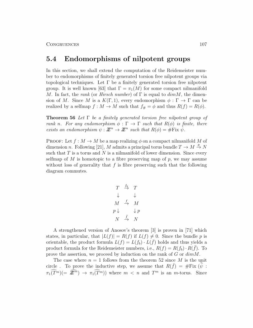
Congruences 107

5.4 Endomorphisms of nilpotent groups

In this section, we shall extend the computation of the Reidemeister num-ber to endomorphisms of finitely generated torsion free nilpotent groups viatopological techniques. Let Γ be a finitely generated torsion free nilpotentgroup. It is well known [63] that Γ = π1(M) for some compact nilmanifoldM . In fact, the rank (or Hirsch number) of Γ is equal to dimM , the dimen-sion of M . Since M is a K(Γ, 1), every endomorphism φ : Γ → Γ can berealized by a selfmap f :M →M such that f# = φ and thus R(f) = R(φ).

Theorem 56 Let Γ be a finitely generated torsion free nilpotent group ofrank n. For any endomorphism φ : Γ → Γ such that R(φ) is finite, thereexists an endomorphism ψ : ZZn → ZZn such that R(φ) = #Fix ψ.

Proof: Let f :M →M be a map realizing φ on a compact nilmanifoldM ofdimension n. Following [21],M admits a principal torus bundle T → M

p→ N

such that T is a torus and N is a nilmanifold of lower dimension. Since everyselfmap of M is homotopic to a fibre preserving map of p, we may assumewithout loss of generality that f is fibre preserving such that the followingdiagram commutes.

Tfb→ T

↓ ↓

Mf→ M

p ↓ ↓ p

Nf→ N

A strengthened version of Anosov’s theorem [3] is proven in [71] whichstates, in particular, that |L(f)| = R(f) if L(f) 6= 0. Since the bundle p isorientable, the product formula L(f) = L(fb) · L(f) holds and thus yields aproduct formula for the Reidemeister numbers, i.e., R(f) = R(fb) ·R(f). Toprove the assertion, we proceed by induction on the rank of G or dimM .

The case where n = 1 follows from the theorem 52 since M is the unitcircle . To prove the inductive step, we assume that R(f) = #Fix ( ψ :π1(Tm)(= ZZm) → π1(Tm)) where m < n and Tm is an m-torus. Since

Congruences 108

R(fb) = #Fix (φb :π1(T ) → π1(T )), if L(f) 6= 0 then the product formula

for Reidemeister numbers gives

R(f) = #Fix (φb) ·#Fix ( ψ)= #Fix (ψ)

where ψ = φb × ψ : π1(Tn) = π1(T ) × π1(T

m) → π1(T ) × π1(Tm) with

T n = T × Tm.

5.5 Main Theorem

The following lemma is useful for calculating Reidemeister numbers. It willalso be used in the proof of the Main Theorem

Lemma 33 Let φ : G → G be any endomorphism of any group G, and letH be a subgroup of G with the properties

φ(H) ⊂ H

∀x ∈ G ∃n ∈ IN such that φn(x) ∈ H.

ThenR(φ) = R(φH),

where φH : H → H is the restriction of φ to H.

Proof Let x ∈ G. Then there is an n such that φn(x) ∈ H . FromLemma 7 it is known that x is φ-conjugate to φn(x). This means that theφ-conjugacy class xφ of x has non-empty intersection with H .

Now suppose that x, y ∈ H are φ-conjugate, ie. there is a g ∈ G suchthat

gx = yφ(g).

We shall show that x and y are φH-conjugate, ie. we can find a g ∈ Hwith the above property. First let n be large enough that φn(g) ∈ H . Thenapplying φn to the above equation we obtain

φn(g)φn(x) = φn(y)φn+1(g).

Congruences 109

This shows that φn(x) and φn(y) are φH-conjugate. On the other hand, oneknows by Lemma 7 that x and φn(x) are φH-conjugate, and y and φn(y) areφH conjugate, so x and y must be φH-conjugate.

We have shown that the intersection with H of a φ-conjugacy class in Gis a φH-conjugacy class in H . We therefore have a map

Rest : R(φ) → R(φH)xφ 7→ xφ ∩H

This clearly has the two-sided inverse

xφH7→ xφ.

Therefore Rest is a bijection and R(φ) = R(φH).

Corollary 19 Let H = φn(G). Then R(φ) = R(φH).

Let µ(d), d ∈ IN be the Moebius function, i.e.

µ(d) =

1 if d = 1,(−1)k if d is a product of k distinct primes,0 if d is not square − free.

Theorem 57 (Congruences for the Reidemeister numbers) Let φ : G→ G be an endomorphism of the group G such that all numbers R(φn) arefinite and let H be a subgroup of G with the properties

φ(H) ⊂ H

∀x ∈ G ∃n ∈ IN such that φn(x) ∈ H.

If one of the following conditions is satisfied:(I) H is finitely generated Abelian,(II) H is finite,(III) H is a direct sum of a finite group and a finitely generated free Abeliangroup,or more generally(IV) H is finitely generated almost Abelian group,

Congruences 110

or(V) H is finitely generated, nilpotent and torsion free , then one has for allnatural numbers n,

∑

d|nµ(d) · R(φn/d) ≡ 0 mod n.

Proof From theorems 52, 55, 56 and lemma 33 it follows immediatelythat , in cases I - IV, for every n

R(φn) = #Fix[φH

n: H → H

].

Let Pn denote the number of periodic points of φH of least period n. Onesees immediately that

R(φn) = #Fix[φH

n]=∑

d|nPd.

Applying Mobius’ inversion formula, we have,

Pn =∑

d|nµ(d)R(φn/d).

On the other hand, we know that Pn is always divisible be n, because Pn isexactly n times the number of φH-orbits in H of length n. In the case V whenH is finitely generated, nilpotent and torsion free ,we know from theorem 56that there exists an endomorphism ψ : Zn → Zn such that R(φn) = #Fix ψn.The proof then follows as in previous cases.

Remark 12 For finite groups, congruences for Reidemeister numbers followfrom those of Dold for Lefschetz numbers since we have identified in remark 2the Reidemeister numbers with the Lefschetz numbers of induced dual maps.


of a continuous map

Using corollary 1 we may apply the theorem 57 to the Reidemeister numbersof continuous maps.

Congruences 111

Theorem 58 Let f : X → X be a self-map such that all numbers R(fn)are finite.Let f∗ : π1(X) → π1(X) be an induced endomorphism of the groupπ1(X) and let H be a subgroup of π1(X) with the properties

f∗(H) ⊂ H

∀x ∈ π1(X) ∃n ∈ IN such that fn∗ (x) ∈ H.

If one of the following conditions is satisfied :(I) H is finitely generated Abelian,(II) H is finite,(III) H is a direct sum of a finite group and a finitely generated free Abeliangroupor more generally,(IV) H is finitely generated almost Abelian group,or(V) H is finitely generated, nilpotent and torsion free ,then one has for all natural numbers n,

∑

d|nµ(d) · R(fn/d) ≡ 0 mod n.


of equivariant group endomorphisms

Let G be a compact Abelian topological group acting on a topological groupπ as automorphisms of π, i.e., a homomorphism ν : G → Aut(π). For everyσ ∈ π, the isotropy subgroup of σ is given by Gσ = g ∈ G|g(σ) = σ whereg(σ) = ν(g)(σ). For any closed subgroup H ≤ G, the fixed point set of theH-action, denoted by

πH = σ ∈ π|h(σ) = σ, ∀h ∈ H,

is a subgroup of π. Since G is Abelian, G acts on πH as automorphisms ofπH . Denote by C(π) (and C(πH)) the set of conjugacy classes of elementsof π (and πH , respectively). Note that the group G acts on the conjugacyclasses via

< σ > 7→< g(σ) >

Congruences 112

for < σ >∈ C(π) (or C(πH)).

Let EndG(π) be the set of G-equivariant endomorphisms of π. For anyφ ∈ EndG(π) and H ≤ G, φH ∈ EndG(π

H) where φH = φ|πH : πH → πH .Furthermore, φ induces a G-map on C(π) defined by

φconj : C(π) → C(π)

via< σ > 7→< φ(σ) > .

Similarly, φH induces

(φH)conj : C(πH) → C(πH).

In the case where π is Abelian, G acts on π via

χ(σ) 7→ χ(g(σ))

for any χ ∈ π, g ∈ G. Thus the dual φ of φ ∈ EndG(π) is also G-equivariant,

i.e., φ ∈ EndG(π). Similarly, φH ∈ EndG(πH).

To establish the congruence relations in this section, we need the followingbasic counting principle.

Lemma 34 Let G be an Abelian topological group and Γ be a G-set withfinite isotropy types. For any G-map ψ : Γ → Γ,

Fix ψ =⊔

K∈Iso(Γ)Fix ψK

where Iso(Γ) is the set of isotropy types of Γ, ΓK = γ ∈ Γ|Gγ = K, ψK =ψ|ΓK : ΓK → ΓK and Fix ψK = (Fix ψ)∩ΓK. In particular, if #Fix ψ <∞then

#Fix ψ =∑

K∈Iso(Γ)#Fix ψK . (5.2)

Congruences 113

Proof: It follows from the decomposition

Γ =⊔

K∈Iso(Γ)ΓK .

Remark Suppose that G is a compact Abelian Lie group. If Fix ψ is finitethen it follows that #Fix ψK = I(ψK), the fixed point index of ψK which isdivisible by χ(G/K), the Euler characteristic of G/K (see [79], [59], [96]).

Theorem 59 Let G be an Abelian compact Lie group. For any subgroupH ∈ Iso(π) and φ ∈ EndG(π), if

(I) π is finitely generated and φ is eventually commutative or(II) π is finite or (III) π is finitely generated torsion free nilpotent, then

∑

H≤K∈Iso(π)µ(H,K)R(φK) ≡ 0 mod χ(G/H)

and ∑

H≤K∈Iso(π)ϕ(H,K)R(φK) ≡ 0 mod χ(G/H)

where µ(, ) denotes the Mobius function on Iso(π) and

ϕ(H,K) =∑

H≤L≤K

χ(L/H)µ(L,K).

Proof: (I): Since φ is eventually commutative, so is φH for every H ≤ G.With the canonical G-action on H1(π), H1(φ) is a G-equivariant endomor-phism of H1(π). Similarly, we have H1(φ

H) ∈ EndG(H1(πH)) and hence

H1(φH) ∈ EndG(H1(πH)). It follows from theorem 52 and formula (5.1) that

R(φH) = #Fix ( H1(φH)) =∑

H≤K∈Iso(π)#Fix ( H1(φH))K .

Hence, by Mobius inversion [2], we have

∑

H≤K∈Iso(π)µ(H,K)R(φK) = #Fix ( H1(φK))H ≡ 0 mod χ(G/H).

Congruences 114

(II): Following theorem 14 , we have

R(φH) = #Fix (φH)conj =∑

H≤K∈Iso(π)#Fix ((φH)conj)K .

The assertion follows from formula (5.1) and the Mobius inversion for-mula.

(III): The commutative diagram in the proof of Theorem 56 gives rise to thefollowing commutative diagram in which the rows are short exact sequencesof groups where π′ is free abelian and π is nilpotent.

1 → π′ i∗→ πp∗→ π → 1

↑ φ′ ↑ φ ↑ φ

1 → π′ i∗→ πp∗→ π → 1

Note that G acts on both π′ and π as automorphisms and so φ′ andφ are both G-equivariant. Similarly, we have φ′H ∈ EndG(π

′H) and φH ∈EndG(φ

H). It follows from the proof of Theorem 56 that the endomorphismψ can be made G-equivariant by the diagonal action on the product of thefibre and the base. Hence,

R(φH) = #Fix ψH =∑

H≤K∈Iso(π)#Fix (ψH)K .

Again, the assertion follows from Mobius inversion.Finally, for the congruences with ϕ(, ), we proceed as in Theorem 6 of

[59].

Remark 13 In [59], Komiya considered the G-invariant set X(H) = GXH

for arbitrary G (not necessarily Abelian). In our case, π(H) need not be asubgroup of π. For example, take π = G = S3 to be the symmetric group onthree letters and let G act on π via conjugation. For any subgroup H ≤ G oforder two, it is easy to see that π(H) is not a subgroup of π.

Congruences 115


of equivariant maps

Unlike Komiya’s generalization [59] of Dold’s result, the congruence rela-tions among the Reidemeister numbers of fn established in section cannotbe generalized without further assumptions as we illustrate in the followingexample.

Example 9 Let X = S2 ⊂ R3, G = Z2 act on S2 via

ζ(x1, x2, x3) = (x1, x2, ζx3)

so that XG = S1. Let f : X → X be defined by (x1, x2, x3) 7→ (−x1, x2, x3).It follows that

R(f) = 1; R(fG) = 2.

Hence, ∑

(1)≤K

µ((1), K)R(fK) = µ(1)R(f) + µ(2)R(fG) = −1

which is not congruent to 0 mod 2.

In order to apply the previous result , we need R(fH) = R((f∗)H), for all

H ≤ G. In the above example, R(fG) = 2 but R((f∗)G) = 1.

Recall that a selfmap f : X → X is eventually commutative [51] if theinduced homomorphism f∗ : π1(X) → π1(X) is eventually commutative. Thefollowing is immediate from Theorem 59.

Theorem 60 Let f : X → X be a G-map on a finite G-complex X whereG is an abelian compact Lie group, such that XH is connected for all H ∈Iso(X). If f is eventually commutative, or π1(X

H) is finite or nilpotent, andR(fH) = R((f∗)

H) for all H ∈ Iso(X), then∑

H≤K∈Iso(π)µ(H,K)R(fK) ≡ 0 mod χ(G/H)

and ∑

H≤K∈Iso(π)ϕ(H,K)R(fK) ≡ 0 mod χ(G/H).

Congruences 116

5.9 Congruences for Nielsen numbers of a con-

tinuous map

Theorem 61 Suppose that there is a natural number m such that fm∗ (π) ⊂

I(fm) . If for every d dividing a certain natural number n we have L(fn/d) 6=0, then one has for that particular n,

∑

d|nµ(d)N(fn/d) ≡ 0 mod n.

Proof From the results of Jiang [51] we have that N(fn/d) = R(fn/d) forthe same particular n and f∗ is eventually commutative. The result nowfollows from theorem 58.

Corollary 20 Let I(idX) = π and for every d dividing a certain naturalnumber n we have L(fn/d) 6= 0, then theorem 61 applies

Corollary 21 Suppose that X is aspherical, f is eventually commutativeand for every d dividing a certain natural number n we have L(fn/d) 6= 0,then theorem 61 applies

Example 10 Let f : T n → T n be a hyperbolic endomorphism. Then forevery natural n ∑


Example 11 Let g : M → M be an expanding map [86] of the orientablesmooth compact manifoldM .ThenM is aspherical and is a K(π1(M), 1), andπ1(M) is torsion free [86].According to Shub [86] any lifting g of g has exactlyone fixed point.From this and the covering homotopy theorem it follows thatthe fixed point of g are pairwise inequivalent.The same is true for all iteratesgn.Therefore N(gn) = #Fix (gn) for all n.So the sequence of the Nielsennumbers N(gn) of an expanding map satisfies the congruences as above.

Congruences 117

Theorem 62 Let X be a connected, compact polyhedron with finite funda-mental group π. Suppose that the action of π on the rational homology ofthe universal cover X is trival, i.e. for every covering translation α ∈ π,α∗ = id : H∗(X, QI) → H∗(X, QI). If for every d dividing a certain naturalnumber n we have L(fn/d) 6= 0, then one has for that particular n,

∑


Proof From the results of Jiang [51] we have that N(fn/d) = R(fn/d) forthe same particular n.The result now follows from theorem 58.

Lemma 35 Let X be a polyhedron with finite fundamental group π and letp : X → X be its universal covering. Then the action of π on the rationalhomology of X is trivial iff H∗(X ;QI) ∼= H∗(X ;QI).

Corollary 22 Let X be a compact 1-connected polyhedron which is a rationalhomology n-sphere, where n is odd. Let π be a finite group acting freely onX and let X = X/π. Then theorem 62 applies.

Proof The projection p : X → X = X/π is a universal covering space ofX . For every α ∈ π, the degree of α : X → X must be 1, because L(α) = 0(α has no fixed points). Hence α∗ = id : H∗(X;QI) → H∗(X ;QI).

Corollary 23 If X is a closed 3-manifold with finite π, then theorem 62applies.

Proof X is an orientable, simply connected manifold, hence a homology3-sphere. We apply corollary 22.

Example 12 Let X = L(m, q1, . . . , qr) be a generalized lens space and f :X → X a continuous map with f1∗(1) = k where | k |6= 1. Then for everynatural n ∑


Congruences 118

Proof

By corollary we see that theorem applies for lens spaces. Since π1(X) =ZZ/mZZ, the map f is eventually commutative. A lens space has a structureas a CW complex with one cell ei in each dimension 0 ≤ i ≤ 2n + 1. Theboundary map is given by ∂e2k = m.e2k−1 for even cells, and ∂e2k+1 = 0 forodd cells. From this we may calculate the Lefschetz numbers:

L(fn) = 1− k(l+1)n 6= 0.

This is true for any n as long as | k |6= 1. The result now follows fromtheorem .

Remark 14 It is known that in previous example

N(fn) = R(fn) = #Coker (1− fn1∗) = hcf(1− kn, m)

for every n.So we obtain pure arithmetical fact: the sequence n 7→ hcf(1 −kn, m) satisfies congruences above for every natural n if | k |6= 1.

5.10 Some conjectures for wider classes of

groups

For the case of almost nilpotent groups (ie. groups with polynomial growth,in view of Gromov’s theorem [44]) we believe that the congruences for theReidemeister numbers are also true.We intend to prove this conjecture byidentifying the Reidemeister number on the nilpotent part of the group withthe number of fixed points in the direct sum of the duals of the quotientsof successive terms in the central series. We then hope to show that theReidemeister number of the whole endomorphism is a sum of numbers oforbits of such fixed points under the action of the finite quotient group (iethe quotient of the whole group by the nilpotent part). The situation forgroups with exponential growth is very different. There one can expect theReidemeister number to be infinite as long as the endomorphism is injective.

Chapter 6

The Reidemeister torsion

6.1 Preliminaries

Like the Euler characteristic, the Reidemeister torsion is algebraically de-fined. Roughly speaking, the Euler characteristic is a graded version of thedimension, extending the dimension from a single vector space to a complexof vector spaces. In a similar way, the Reidemeister torsion is a graded ver-sion of the absolute value of the determinant of an isomorphism of vectorspaces: for this to make sense, both vector spaces should be equipped witha positive density.

Recall that a density f on a complex space V of dimension n is a mapf : ∧nV → R with f(λ · x) = |λ| · f(x) for all x ∈ ∧nV, λ ∈ CI. Thedensities on V clearly form a real vector space |V | of dimension one. If f isnonzero and takes values in [o,∞), we say that it is positive . If V1 and V2are both n-dimensional and A : V1 → V2 is linear over CI, then there is aninduced map A∗ : |V2| → |V1|. If each Vi carries a preffered positive densityfi then A∗f2 = a · f1, for some a ≥ 0, and we write a = |detA|.In the caseV1 = V2, f1 = f2 then a is indeed the absolute value of the determinant of A,so this notation is consistent.

If 0 → V1 → V2 → V3 → 0 is an exact sequence of finite dimensionalvector spaces over CI , then there is a natural isomorphism ∧n1V1 ⊗∧n3V3 →∧n2V2, ni = dimVi.This induces a natural isomorphism |V1| ⊗ |V3| ∼= |V2|. IfV is zero, then absolute value is a standard generator for |V | and sets up anatural isomorphism |V | ∼= R.

119

Reidemeister torsion 120

Let di : C i → C i+1 be a cochain complex of finite-dimensional vectorspaces over CI with C i = 0 for i < 0 or i large. Let Z i = kerdi, Bi =imdi−1, and H i = Z i/Bi be the cocycles, coboundaries, and cohomology ofC∗ respectively. If one is given positive densities ∆i on C

i and Di on Hi(with

the standard choice when i is negative or large), then the Reidemeister torsionτ(C∗,∆i, Di) ∈ (0,∞) is defined as follows. The short exact sequences 0 →Z i → C i → Bi+1 → 0 and 0 → Bi → Z i → H i → o together with thetrivializations |C i| = R ·∆i, |H

i| = R ·Di give isomorphisms |Z i| ⊗ |Bi+1| ∼=R, |Bi| ∼= |Z i| for each i. This gives isomorphisms |Bi| ⊗ |Bi+1| ∼= R, hencealso |Bi| ∼= |Bi+2|. But for i ≤ 0 or i large, Bi = 0 and so |Bi| = R. Soif j is large and even, we find R = |Bj| ∼= |B0| = R and this isomorphismis the multiplication by scalar τ ∈ R∗. This is the Reidemeister torsionτ(C∗,∆i, Di).

If the cohomology H i = 0 for all i we say that C∗ is acyclic and we writeτ(C∗,∆i) for the torsion when all the Di are standard .

When C∗ is acyclic , there is another way to define τ .

Definition 15 Consider a chain contraction δi : C i → C i−1, i.e. a linearmap such that d δ + δ d = id. Then d+ δ determies a map

(d+ δ)+ : C+ := ⊕C2i → C− := ⊕C2i+1 and a map (d+ δ)− : C− → C+.Since the map (d+δ)2 = id+δ2 is unipotent, (d+δ)+ must be an isomorphism.One defines τ(C∗,∆i) :=| det(d+ δ)+ | (see [42]).

Reidemeister torsion is defined in the following geometric setting. Sup-pose K is a finite complex and E is a flat, finite dimensional, complex vectorbundle with base K. We recall that a flat vector bundle over K is essentiallythe same thing as a representation of π1(K) when K is connected. If p ∈ K isa basepoint then one may move the fibre at p in a locally constant way arounda loop in K. This defines an action of π1(K) on the fibre Ep of E above p. Wecall this action the holonomy representation ρ : π → GL(Ep). Conversely,given a representation ρ : π → GL(V ) of π on a finite dimensional complexvector space V , one may define a bundle E = Eρ = (K×V )/π. Here K is theuniversal cover of K, and π acts on K by covering tranformations and on Vby ρ. The holonomy of Eρ is ρ, so the two constructions give an equivalenceof flat bundles and representations of π.

If K is not connected then it is simpler to work with flat bundles. Onethen defines the holonomy as a representation of the direct sum of π1 of the


components of K. In this way, the equivalence of flat bundles and represen-tations is recovered.

Suppose now that one has on each fibre of E a positive density which islocally constant on K. In terms of ρE this assumption just means | det ρE |=1. Let V denote the fibre of E. Then the cochain complex C i(K;E) withcoefficients in E can be identified with the direct sum of copies of V associatedto each i-cell σ of K. The identification is achieved by choosing a basepointin each component of K and a basepoint from each i-cell. By choosing a flatdensity on E we obtain a preferred density ∆i on C

i(K,E). Let H i(K;E) bethe i-dimensional cohomology of K with coefficients in E , i.e. the twistedcohomology of E. Given a density Di on each H i(K;E), one defines theReidemeister torsion of (K;E,Di) to be τ(K;E,Di) = τ(C∗(K;E),∆i, Di) ∈(0,∞). A case of particular interest is when E is an acyclic bundle, meaningthat the twisted cohomology of E is zero (H i(K;E) = 0), then one can takeDi to be the absolute value map on ∧0(0) = CI and the resulting Reidemeistertorsion is denoted by τ(K;E). In this case it does not depend on the choiceof flat density on E.

The Reidemeister torsion of an acyclic bundle E on K has many niceproperties. Suppose that A and B are subcomplexes of K. Then we have amultiplicative law:

τ(A ∪B;E) · τ(A ∩B;E) = τ(A;E) · τ(B;E) (6.1)

that is interpreted as follows. If three of the bundles E|A ∪ B, E|A ∩B, E|A, E|B are acyclic then so is the fourth and the equation (6.1) holds.

Another property is the simple homotopy invariance of the Reidemeistertorsion. SupposeK ′ is a subcomplex ofK obtained by an elementary collapseof an n-cell σ in K. This means that K = K ′ ∪ σ ∪ σ′ where σ′ is an (n− 1)cell of K so set up that ∂σ′ = σ′ ∩K ′ and σ′ ⊂ ∂σ, i.e. σ′ is a free face of σ.So one can push σ′ through σ into K ′ giving a homotopy equivalence.ThenH∗(K;E) = H∗(K ′;E) and

τ(K;E,Di) = τ(K ′;E,Di) (6.2)

By iterating a sequence of elementary collapses and their inverses, one obtainsa homotopy equivalence of complexes that is called simple . Plainly onehas,by iterating (6.2) , that the Reidemeister torsion is a simply homotopyinvariant. In particular τ is invariant under subdivision. This implies that


for a smooth manifold, one can unambiguously define τ(K;E,Di) to be thetorsion of any smooth triangulation of K.

In the case K = S1 is a circle, let A be the holonomy of a generator of thefundamental group π1(S

1). One has that E is acyclic iff I − A is invertibleand then

τ(S1;E) =| det(I −A) | (6.3)

Note that the choice of generator is irrelevant as I − A−1 = (−A−1)(I − A)and |det(−A−1| = 1.

These three properties of the Reidemeister torsion are the analogues ofthe properties of Euler characteristic ( cardinality law, homotopy invarianceand normalization on a point), but there are differences.Since a point has noacyclic representations (H0 6= 0) one cannot normalise τ on a point as wedo for the Euler characteristic, and so one must use S1 instead. The multi-plicative cardinality law for the Reidemeister torsion can be made additivejust by using log τ , so the difference here is inessential. More important forsome purposes is that the Reidemeister torsion is not an invariant under ageneral homotopy equivalence: as mentioned earlier this is in fact why it wasfirst invented.

It might be expected that the Reidemeister torsion counts somethinggeometric(like the Euler characteristic). D. Fried showed that it counts theperiodic orbits of a flow and the periodic points of a map. We will show thatthe Reidemeister torsion counts the periodic point classes of a map( fixedpoint classes of the iterations of the map).

Some further properties of τ describe its behavior under bundles.Let p : X → B be a simplicial bundle with fiber F where F,B,X are

finite complexes and p−1 sends subcomplexes of B to subcomplexes of X .over the circle S1. We assume here that E is a flat, complex vector bundleover B . We form its pullback p∗E over X . Note that the vector spacesH i(p−1(b), CI) with b ∈ B form a flat vector bundle over B, which we denoteH iF . The integral lattice in H i(p−1(b), IR) determines a flat density by thecondition that the covolume of the lattice is 1. We suppose that the bundleE ⊗H iF is acyclic for all i. Under these conditions D. Fried [42] has shownthat the bundle p∗E is acyclic, and

τ(X ; p∗E) =∏

i

τ(B;E ⊗H iF )(−1)i . (6.4)


the opposite extreme is when one has a bundle E on X for which the restric-tion E|F is acyclic. Then, for B connected,

τ(X ;E) = τ(F ;E|F )χ(B) (6.5)

Suppose in (6.5) that F = S1 i.e. X is a circle bundle . Then (6.5) can beregarded as saing that

log τ(X ;E) = χ(B) · log τ(F ;E|F )

is counting the circle fibers in X in the way that χ counts points in B, witha weighting factor of log τ(F ;E|F ).

6.2 The Reidemeister zeta Function and the

Reidemeister Torsion of the Mapping To-

rus of the dual map.

Let f : X → X be a homeomorphism of a compact polyhedron X . LetTf := (X × I)/(x, 0) ∼ (f(x), 1) be the mapping tori of f . We shall considerthe bundle p : Tf → S1 over the circle S1. We assume here that E is aflat, complex vector bundle with finite dimensional fibre and base S1. Weform its pullback p∗E over Tf . Note that the vector spaces H

i(p−1(b), c) withb ∈ S1 form a flat vector bundle over S1, which we denote H iF . The integrallattice in H i(p−1(b), IR) determines a flat density by the condition that thecovolume of the lattice is 1. We suppose that the bundle E ⊗H iF is acyclicfor all i. Under these conditions D. Fried [42] has shown that the bundle p∗Eis acyclic, and we have

τ(Tf ; p∗E) =

∏

i

τ(S1;E ⊗H iF )(−1)i . (6.6)

Let g be the prefered generator of the group π1(S1) and let A = ρ(g) where

ρ : π1(S1) → GL(V ). Then the holonomy around g of the bundle E ⊗H iF

is A⊗ f ∗i .

Since τ(S1;E) =| det(I −A) | it follows from (6.6) that

τ(Tf ; p∗E) =

∏

i

| det(I − A⊗ f ∗i ) |

(−1)i . (6.7)


We now consider the special case in which E is one-dimensional, so A is justa complex scalar λ of modulus one. Then in terms of the rational functionLf (z) we have [42]:

τ(Tf ; p∗E) =

∏

i

| det(I − λ · f ∗i ) |

(−1)i=| Lf(λ) |−1 (6.8)

Theorem 63 Let φ : G→ G be an automorphism of G,where G is the directsum of a finite group with a finitely generated free Abelian group, then

τ(Tφ; p

∗E)=| Lφ(λ) |

−1=| Rφ(σ · λ) |(−1)r+1

, (6.9)

where λ is the holonomy of the one-dimensional flat complex bundle E overS1, r and σ are the constants described in theorem 13 .

Proof We know from the theorem 52 that R(φn) is the number of fixedpoints of the map φn. In general it is only necessary to check that the numberof fixed points of φn is equal to the absolute value of its Lefschetz number.We assume without loss of generality that n = 1. We are assuming that R(φ)is finite, so the fixed points of φ form a discrete set. We therefore have

L(φ) =∑

x∈Fix φ

Index (φ, x).

Since φ is a group endomorphism, the trivial representation x0 ∈ G is alwaysfixed. Let x be any fixed point of φ.Since G is union of tori G0, ..., Gt and φis a linear map, we can shift any two fixed points onto one another withoutaltering the map φ. This gives us for any fixed point x the equality

Index (φ, x) = Index (φ, x0)

and so all fixed points have the same index. It is now sufficient to show thatIndex (φ, x0) = ±1. This follows because the map on the torus

φ : G0 → G0

lifts to a linear map of the universal cover, which is an euclidean space. Theindex is then the sign of the determinant of the identity map minus thislifted map. This determinant cannot be zero, because 1− φ must have finitekernel by our assumption that the Reidemeister number of φ is finite (ifdet(1− φ) = 0 then the kernel of 1− φ is a positive dimensional subspace ofG, and therefore infinite).


Corollary 24 Let f : X → X be a homeomorphism of a compact polyhedronX. If π1(X) is the direct sum of a finite group with a free Abelian group,then then

τ(T(f1∗)

; p∗E)=

∣∣∣∣ L(f1∗)(λ)

∣∣∣∣−1

=∣∣∣ Rf(σ · λ)

∣∣∣(−1)r+1

,

where r and σ are the constants described in theorem 13 .

6.3 The connection between the Reidemeis-

ter torsion, eta–invariant, the Rochlin in-

variant and theta multipliers via the dy-

namical zeta functions

In this section we establish a connection between the Reidemeister torsionof a mapping tori, the eta-invariant, the Rochlin invariant, and theta multi-pliers via the Lefchetz zeta function and the Bismut-Freed-Witten holonomytheorem.

6.3.1 Rochlin invariant

We begin by recalling the definition of a spin structure on an oriented Rie-mannian manifold Mm with special attention to the notion of a spin diffeo-morphism. The tangent bundle TM is associated to a principal GL+(m)bundle P , the bundle of oriented tangent frames. This last group GL+(m)has a unique connected two-fold covering group GL+(m). If the tangentbundle TM is associated to a princial GL+(m) bundle P , then we call P aspin structure on M . Thus, spin structures are in one-to-one correspondencewith double coverings P → P which are nontrivial on each fiber. In terms ofcohomology, such coverings are given by elements w of H1(P, ZZ/2ZZ) suchthat w | π−1(x) = 0 for every x in M , where π : P → M is the bundleprojection and π−1(x) is the fiber over x. We shall refer to the cohomologyclass w as a spin structure on M , and the pair (M,w) as a spin manifold.

Given an orientation preserving diffeomorphism f :M →M , the differen-tial df of f gives us a diffeomorphism df : P → P and hence an isomorphismon the cohomology (df)∗ : H1(P, ZZ/2ZZ) → H1(P, ZZ/2ZZ). We say that an


orientation-preserving diffeomorphism f : M → M preserves the spin struc-ture w if (df)∗(w) = w in H1(P, ZZ/2ZZ). This is equivalent to the existenceof a bundle map b : P → P making the following diagram commutative

Pb→ P

↓ ↓

Pdf→ P

By a spin diffeomorphism F of (M,w) we mean a pair F = (f, b) consistingnot only of a spin preserving diffeomorphism f but also of a bundle mapb : P → P covering df . Given a spin diffeomorphism F = (f, b) of (M,w)there is a well defined spin structure w′ on the mapping torus Tf (see [61]).

We shall now define an invariant of spin diffeomorphisms F of (M,w)where M has dimension 8k + 2. This will actually be defined via (Tf , w

′),a spin manifold of dimension 8k + 3. As usual, a spin manifold (N8k+3, w)is a spin boundary if there is a compact 8k + 4-dimensional spin manifold(X8k+4,W ) with ∂X = N and with W restricting to w. By a result of [3]the manifold N8k+3 is a spin boundary if and only if it is an unorientedboundary. A necessary and sufficient condition for N to be a boundary isthat all its Stiefel-Whitney numbers vanish. In particular, this is alwaysthe case when k = 0 or k = 1. If M8k+2 has vanishing Stiefel-Whitneyclasses, then all the Stiefel-Whitney numbers of Tf are zero (see [61]). For aspin boundary (N8k+3, w) = ∂(X8k+4,W ) the Rochlin invariant R(N,w) inZZ/16ZZ is defined by

R(N,w) ≡ σ(X) (mod 16),

where σ(X) denotes the signature of the 8k + 4-dimensional manifold X .

6.3.2 Determinant line bundles, the Eta-invariant andthe Bismut-Freed-Witten theorem

Let π : Z → N be a smooth fibration of manifolds with base manifold N andtotal manifold Z. The fiber above a point x ∈ N is an 8k + 2-dimensionalmanifoldM8k+2

x which is equipped with a metric and a compatible spin struc-ture. The latter vary smoothly with respect to the parameter x in the basemanifold; in other words the structure group of the fibration π : Z → N is asubgroup of the spin diffeomorphism group.


In this situation, along a fiber Mx, we have a principal Spin(8k + 2)-bundle P (TMx). Since the dimension 8k + 2 is even there are two half-spin representation S± of Spin(8k + 2) and associated to them two vectorbundles E±

x = P (TMx)⊗S±. On the space C∞(E±x ) of C

∞-sections of thesebundles, there is a Dirac operator ∂x : C∞(E±

x ) → C∞(E∓x ) which is a first

order, elliptic, differential operator [18]. If we replace the C∞-sections ofE±

x by square-integrable sections, the Dirac operator can be extended to anoperator ∂x : L2(E±

x ) → L2(E∓x ) of Hilbert spaces. As we vary x over N ,

these Hilbert spaces L2(E±x ) form Hilbert bundles L2(E±) and the operators

∂x form a continuous family of operators ∂ : L2(E±) → L2(E∓) on theseHilbert bundles.

From the work Atiyah-Singer, Bismut-Freed [9] and Quillen [76] it followsthat there exists a well-defined complex line bundle det ∂ over N . Over apoint x in N , the fiber of this line bundle (det ∂)x is isomorphic to(Λmaxker∂x)

∗⊗(Λmaxcoker∂x). Bismut and Freed [9] undertook an extensivestudy of the geometry of this determinant line bundle det ∂. They showedthat det ∂ admits a Bismut-Freed connection , and proved a formula forthe curvature associated to this connection. One of the basic results in [9] isthe holonomy formula for the Bismut-Freed connection of the determinantline bundle det ∂ around an immersed circle γ : S1 → N in the base manifoldN . We now describe this formula. Pulling back by γ, there is an 8k + 3-dimensional manifold which is diffeomorphic to a mapping torus Tφ, with thediffeomorphism φ specified by γ. Choosing an arbitrary metric gS1 on S1,and using the projection Φ : τ(Tφ) → τfiber(Tφ) of tangent bundles, we obtaina Riemannian structure on Tφ. Since the structure group of the fibrationπ : Z → N is a subgroup of the spin diffeomorphism group, it follows that φis covered by a canonical spin diffeomorphism and the mapping torus Tφ hasa natural spin structure. From this spin structure on Tφ we obtain a spinbundle over Tφ with structure group Spin(8k + 3) and Dirac operator ∂ onthe space of C∞-sections of this bundle.

Following Atiyah, Patodi, Singer [7] we define the function η(s, ∂) in termsof the eigenvalues λ of ∂ by

η(s, ∂) =∑

λ6=0

signλ

| λ |s.

This function is holomorphic for Re(s) > 0 and its value at s = 0 is theη-invariant of ∂: η(∂) = η(0, ∂). We denote by h(∂) the dimension of the


kernel of the operator ∂. Notice that these invariants depend on the choiceof the metric gS1 on the base circle S1. In order to be free of this choice, wescale the metric gS1 by a factor 1

ǫ2, and with respect to this new metric

gS1

ǫ2

we have a Dirac operator ∂ǫ on Tφ and a corresponding η-invariant η(∂ǫ) and

h(∂ǫ). As the parameter ǫ tends to zero, the invariant η(∂ǫ)+h(∂ǫ)2

tends to afixed limit.

Theorem 64 [9] The holonomy of the Bismut-Freed connection of thedeterminant line bundle det ∂ around γ is given by

hol(γ; det ∂,) = limǫ→0

exp

(−2πi

η(∂ǫ) + h(∂ǫ)

2

). (6.10)

Now, suppose that π : Z → N is a fibration of manifolds M8k+2 withtwo prefered spin structures w1 and w2. Corresponding to these two spinstructures, there are families of Dirac operators ∂w1 and ∂w2 , and determinantline bundles det ∂w1 and det ∂w2 . Notice that from the curvature formula ofBismut-Freed [9] these two complex line bundles det ∂w1 and det ∂w2 havethe same curvature 2-form. Hence if we form the bundle det ∂w1/ det ∂w2 =det ∂w1⊗(det ∂w2)

∗, the result is a flat complex line bundle. In the language ofcontemporary physicists, this is known as the cancelation of local anomalies.For some of their models, it is important to investigate the holonomies of theflat line bundle det ∂w1 ⊗ (det ∂w2)

∗ -the global anomalies.Let w′

1 and w′2 be the spin structures on Tφ induced by w1 and w2, where

the diffeomorphism φ is specified by γ. Lee, Miller and Weintraub provedthe following

Theorem 65 ([61]) The holonomy of the flat complex line bundledet ∂w1/ det ∂w2 around a loop γ is

hol(γ; det ∂w1/ det ∂w2) =

= limǫ→0

exp(− 2πi

[η(∂w′1ǫ) + h(∂w′

1ǫ)

2−η(∂w′

2ǫ) + h(∂w′

2ǫ)

2

])

If the fiber M8k+2 is a Riemann surface, then

hol(γ; det ∂w1/ det ∂w2) = exp

[−2πi

R(Tφ, w′1)−R(Tφ, w

′2)

8

].


6.3.3 Connection with Reidemeister torsion

Let us now suppose that F = (f, bi), i = 1, 2 are two spin diffeomorphismsof spin manifolds (M8k+2, wi), i = 1, 2. Then there are well-defined spinstructures w′

i, i = 1, 2 on the mapping torus Tf . We may consider Tf as abundle p : Tf → S1 over the circle S1 with fiber M8k+2. As above we havetwo Dirac operators ∂w′

iǫ, i = 1, 2 on the space of C∞-sections of the spin

bundles over Tf and corresponding eta-invariants η(∂w′iǫ) and h(∂w′

iǫ). We

also have a flat complex determinant line bundle det ∂w1/ det ∂w2 over thebase manifold S1 and its pullback p∗(det ∂w1/ det ∂w2) over Tf . Let γ be thepreferred generator of the fundamental group π1(S

1).

Theorem 66

τ(Tf ; p∗(det ∂w1/ det ∂w2)) =| Lf (λ) |

−1,

whereλ = hol(γ; det ∂w1/ det ∂w2) =

= limǫ→0

exp

(−2πi

[η(∂w′

1ǫ) + h(∂w′

1ǫ)

2−η(∂w′

2ǫ) + h(∂w′

2ǫ)

2

])

If the fiber M8k+2 is a Riemann surface, then

λ = hol(γ; det ∂w1/ det ∂w2) = exp

[−2πi

R(Tf , w′1)− R(Tf , w

′2)

8

]

Proof The connection between the Reidemeister torsion of the mappingtorus and the Lefschetz zeta function follows from formula (6.8):

τ(Tf ; p∗(det ∂w1/ det ∂w2)) =| Lf (λ) |

−1,

whereλ = hol(g; det ∂w1/ det ∂w2)

The result now follows from the previous theorem 65.


6.3.4 The Reidemeister torsion and theta-multipliers

We recall some well known properties of theta-functions (see [54]). Fix an in-teger g ≥ 1. A characteristic m is a row vector m = (m∗

1, ..., m∗g, m

∗∗1 , ..., m

∗∗g )

each of whose entries is zero or one. The parity e(m) = m∗1 ·m

∗∗1 + ...+m∗

g ·m∗∗

g ∈ ZZ/2ZZ of the characteristic m is said to be even (odd) when e(m) = 0(= 1).

Let Sg denote the Siegel space of degree g. We shall write elementsT ∈ Sp2g(ZZ) as block matrices:

T =

(A BC D

).

The theta function with characteristic m is a function θm

: Sg × CIg → CIsatisfying the following transformations law [54] :

θT ·m(z(Cτ +D)−1, (Aτ +B)(Cτ +D)−1) =

= γm(T ) · det(Cτ +D)1/2 · exp

(πiz(Cτ +D)−1 tz

)· θ

m(τ, z)

whereT ·m = m · T−1 + ((D tC)0(B

tA)0) (mod 2)

and ( )0 denotes the row vector obtained by taking the diagonal elements ofthe matrix. The number γ

m(T ) is an eighth root of unity, and are known

as the theta multiplier of T for the characteristic m. The action of thesymplectic group Sp2g(ZZ) on the characteristic (denoted above m 7→ T.m)preserves parity, and is transitive on characteristics of a given parity. Welet Γ(m) = T ∈ Sp2g(ZZ) | T ·m = m. If Γ2 is the principal congruencesubgroup of level 2 in Sp2g(ZZ), i.e.

Γ2 = T ∈ Sp2g(ZZ) | T ≡ I (mod 2),

then Γ2 ⊂ Γ(m) for every m.For a diffeomorphism f : V 2 → V 2 of a Riemann surface V 2 of genus

g, the induced map on the homology T = f∗ : H1(V2, ZZ) → H1(V

2, ZZ) isan element in the integral symplectic group Sp2g(ZZ). There is a bijectionbetween the set of Spin structures on V 2 and the set of characteristics m.We shall let w

mdenote the spin structure corresponding to the characteristic

m. Thus a diffeomorphism f : V 2 → V 2 preserves the spin structure wm

iff


f∗ : H1(V, ZZ) → H1(V, ZZ) is in Γ(m). If f∗ is in Γ2 then f preserves eachof the spin structures on V 2. Let T be any element of Γ2 ⊂ Sp2g(ZZ) andf : V 2 → V 2 be a diffeomorphism with f∗ = T : H1(V

2, ZZ)) → H1(V2, ZZ).

Consider again the bundle p : Tf → S1 over the circle S1 with the fiber V 2.Let w

mand w

nbe two spin structures on V 2 corresponding to any two even

characteristic m and n. We have a flat complex determinant line bundledet ∂wm/ det ∂wn over the base S1 and its pullback p∗(det ∂wm/ det ∂wn) overthe mapping tori Tf .

Theorem 67

τ(Tf ; p∗(det ∂wm/ det ∂wn) =| Lf (γm(T )/γ

n(T )) |−1 .

Proof Lee,Miller and Weintraub [61] proved that

γm(T )/γ

n(T ) = exp

(−2πi

R(Tf , wm)−R(Tf , wn)

8

)

Now the statement of the theorem it follows from theorem 66.

6.4 Topology of an attraction domain and

the Reidemeister torsion

6.4.1 Introduction

Assume that on a smooth compact manifoldM of dimension n there is givena tangential vector field X of class C1, and consider the corresponding systemof differential equations

dx

dt= X(x), (6.11)

Let φ(t, x) is the trajectory of (1) passing through the point x for t = 0. Weshall say that the set I is the attractor or the asymptotically stable compactinvariant set for system (1) if for any neighborhood U of I there is the neigh-borhood W , I ⊂W ⊂ U such that1) for any x ∈ W φ(t, x) ∈ U, if t ∈ [0,+∞),

2) for any x ∈ W φ(t, x) −→ I,when t −→ +∞.


By a Lyapunov function V (x) for attractor I we mean a function thatsatisfies following conditions1)V (x) ∈ C1(U − I), V (x) ∈ C(U),

2)V (x) > 0, x ∈ U − I; V (x) = 0, x ∈ I,

3) The derivative by virtue of the system (1) dV (x)dt

> 0 in U − I.

Such Lyapunov function V (x) for I always exist [100]. Suppose that S is alevel surface of Lyapunov function V (x) in U .The conditions 3) and the Im-plicit Function Theorem imply that the level surface S is a compact smoothn−1-dimensional manifold transverse to the trajectories of (1) and trajecto-ries of (1) intersect S on the descending side of the Lyapunov function V (x).Any two level surfaces of the Lyapunov function V (x) are diffeomorphic.Notethat manifold S is determined up to diffeomorphism by the behavior of tra-jectories of the system (1) in U − I and does not depend on the choice of theLyapunov function V (x) and its level. Let N ⊃ I, dimN = n, be a compactsmooth manifold with the boundary ∂N = S.In this article we will study the dependence of the topology of the attractiondomain

D = x ∈ M − I : φ(t, x) −→ I,when t −→ +∞

of the attractor I and of the level surface S of the Lyapunov function V (x) onthe dynamical properties of the system (1) on the attractor. The investigationof the topological structure of the level surfaces of the Lyapunov function wasinitiated by Wilson [100]. Note that the attraction domainD is diffeomorphicto S × R1,since each trajectory of system (1) in the invariant attractiondomain D intersects n − 1-dimensional manifold S exactly once.Hence itfollows that the homology groups of D and S are isomorphic.

6.4.2 Morse-Smale systems

We assume in this section that system (1) is given in Rn and is a Morse-Smalesystem on manifold N , i.e. the following conditions are satisfied:1) A set of nonwandering trajectories Ω of system (1) is the union of a finitenumber of hyperbolic stationary points and hyperbolic closed trajectories,2) Stable and unstable manifolds of stationary points and closed trajectoriesintersect transversally.


A stable or unstable manifold of a stationary point or a closed trajectoryp is denoted byW s(p) andW u(p). Let ak be the number of stationary pointsp of system (1) in I such that dimW u(p) = k, bk is the number closed orbitsq of system (1) in I such that dimW u(q) = k, Mk = ak + bk + bk+1,Bk = dimHk(D;Q) = dimHk(S;Q), χ(D) = χ(S) is the Euler characteristicof D and S.

Theorem 68 The numbers Bk and Mk satisfy the following inequalities:

B0 ≤M0 +Mn−1 −Mn,

B1 − B0 ≤M1 −M0 +Mn−2 −Mn−1 +Mn,

B2 −B1 +B0 ≤ M2 −M1 +M0 +Mn−3 −Mn−2 +Mn−1 −Mn, (6.12)

.......................................................................................,

n−1∑

i=0

(−1)i · Bi = χ(S) = χ(D) = (1 + (−1)n−1)n∑

i=0

(−1)i ·Mi.

To prove the theorem we need several preliminary definitions and lemmas.

Lemma 36Br = Br(N) +Bn−1−r(N), (6.13)

where Br(N) = dimHr(N ;Q).

Proof It is possible to assume that S lies on the n-dimensional sphereSn.Suppose C = Cl(Sn − N) is the closure of the complement of N . ThenS = C ∩N . The manifolds C and N are compact and intersect only on theboundary. Consequently, we have the exact reduced Maier-Vietoris sequence[79]:

....→ Hr+1(Sn;Q) → Hr(S;Q) → Hr(N ;Q)⊕ Hr(C;Q) → Hr(S

n;Q) → ...

Set 1 ≤ r < n− 1.Then Hr(Sn;Q) = Hr+(S

n;Q) = 0, and therefore

Hr(S;Q) = Hr(N ;Q)⊕ Hr(C;Q).

Hence Br(S) = Br(N)+ Br(C), where Br denotes the dimension of Hr.FromAlexander duality it follows that Br(C) = Br(N − ∂N) It is easy to show


that N and N − ∂N are homotopically equivalent( for example, by means ofthe collar theorem). ThereforeBr(N − ∂N) = Br(N), hence

Br(S) = Br(N) + Bn−1−r(N) and Br(S) = Br(N) + Bn−1−r(N).

The manifold S is closed and orientable ; therefore in case r = n − 1 weobtain the following from Poincare duality:

B0(S) = B0(N) +Bn−1(N).

Thus the lemma is proved for all r = 0, 1, 2, ..., n − 1. We make thefollowing definition:

Definition 16 The stationary point p of the vector fieldX with dimW u(p) =k has standard form if there exist local coordinates x1, x2, ..., xk; y1, y2, .., yn−k

in some neighborhood of the point p such that

X = x1∂

∂x1+ ......+ xk

∂

∂xk− y1

∂

∂y1− ....− yn−k

∂

∂yn−k

in this neighborhood.

The standard form for a closed trajectory is defined analogously [38].

Lemma 37 [38] If X0 is a Morse-Smale vector field on the manifold N , thenthere exists a path in the space of smooth vector fields on N, Xt, t ∈ [0, 1],such that:1) Xt is a Morse-Smale vector field for all t ∈ [0, 1];2) the stationary points and closed trajectories of the field X1 are all instandard form.By using this result we replace the original vector field by a vector field forwhich all stationary points and closed trajectories have standard form.

Lemma 38 [38] Suppose X is a Morse-Smale vector field on an orientablemanifold, γ is a closed trajectory in standard form, dimW u(γ) = k + 1, Uis a sufficiently small neighborhood of γ. There exists a Morse-Smale vectorfield Y which coincides with x outside of U , in U has stationary points p andq, and has no other stationary points or closed orbits.Moreover dimW u(p) =k, dimW u(q) = k + 1.


By means of this lemma we replace a vector field on the manifold Nby the field Y having no closed trajectories.In this connection the numberof stationary points of the field Y with dimW u(p) = k will be equal toak + bk + bk+1

Lemma 39 [88] Suppose Y is a smooth Morse-Smale vector field withoutclosed trajectories on a compact manifold N with boundary, the stationarypoints of Y have standard form, and the vector field on ∂N is directed in-ward. Then there exists a Morse function f on N such that:1) the critical points of the function f coincide with stationary points of thefield Y , the index of a critical point of the function f coincides with the di-mension of the unstable manifold of this point ;2) if p ∈ N is a critical point of f then f(p) = dimW u(p);3) f(∂N) = n+1

2.

Lemma 40 [88] Suppose f is a Morse function on N satisfyingconditions 1) - 3). Then:

B0(N) ≤M0,

B1(N)− B0(N) ≤ M1 −M0,

B2(N)− B1(N) +B0(N) ≤ M2 −M1 +M0, (6.14)

.......................................................................................,n∑

i=0

(−1)i · Bi(N) = χ(N) =n∑

i=0

(−1)i ·Mi.

Corollary 25 The following inequalities hold:

Bn−1(N) ≤Mn−1 −Mn,

Bn−2(N)−Bn−1(N) ≤Mn−2 −Mn−1 +Mn,

Bn−3(N)−Bn−2(N) +Bn−1(N) ≤Mn−3 −Mn−2 +Mn−1 −Mn, (6.15)

.......................................................................................,n−1∑

i=0

(−1)i ·Bi(N) = χ(N) = (1 + (−1)n−1)n−1∑

i=0

(−1)i ·Mi.


Proof of the corollary. From the fact that Hn(N) = 0 it follows that

−Bn−1(N) +Bn−2(N)...+ (−1)nB0(N) =Mn −Mn−1...+ (−1)nM0 (6.16)

Adding (6.16) to the inequalities (6.14) and subtracting (6.16) from the in-equalities (6.14) we obtain system of the inequalities (6.15).

Proof of Theorem 68 From lemma 1, inequalities (6.14) and (6.15)it follows that

Bk −Bk−1+Bk−2− ...+ (−1)kB0 = Bk(N)−Bk−1(N) + ...+ (−1)kB0(N) +

+Bn−1−k(N)−Bn−k(N) +Bn−k+1(N) + .... + (−1)kBn−1(N) ≤

≤Mk−Mk−1+......+(−1)kM0+Mn−1−k−Mn−k+......+(−1)kMn−1−(−1)kMn;

χ(S) =n−1∑

k=0

(−1)k · Bk =n−1∑

k=0

(−1)k(Bk(N) +Bn−1−k(N)).

Using the fact that Hn(N) = 0 and changing the index of summation weobtain

χ(S) = (1 + (−1)n−1)n∑

i=0

(−1)i · Bi(N) = (1 + (−1)n−1)n∑

i=0

(−1)i ·Mi

The theorem is proved.

6.4.3 A formula for the Euler characteristic

The last identity in Theorem 68 is also true in more general situation.Namely, assume that system (6.11) is an autonomous system of differentialequations having a finite number of stationary points in attractor I. Denoteby Index (p) the indices of the vector field X at stationary point p.

Theorem 69

χ(D) = χ(S) = ((−1)n − 1) ·∑

p∈IIndex (p). (6.17)


Proof The vector field X is directed on ∂N into N . Therefore from thePoincare-Hopf theorem [65], by replacing X by −X we obtain

χ(N) = (−1)n ·∑

p∈Iind(p).

It is known that χ(∂N) = (1 + (−1)n−1) · χ(N). Hence

χ(D) = χ(S) = ((−1)n − 1) ·∑

p∈IIndex (p).

Corollary 26 Suppose the stationary points on I are hyperbolic , ak is thenumber of stationary points of I with dimW u(p) = k.Since for a hyperbolicstationary point p with dimW u(p) = k the index of the vector field at it isequal to (−1)k, we obtain the following formula:

χ(D) = χ(S) = ((−1)n − 1) ·n∑

k=0

(−1)k · ak. (6.18)

For n = 3 S is union of finite number of spheres with handles.Suppose m isthe number of connected components, p is the total number of handles of themanifold S. Then χ(S) = 2m− 2p. Hence we obtain

Corollary 27m− p = −

∑

p∈IIndex (p). (6.19)

In the case, when stationary points are hyperbolic

m− p = ao − a1 + a2 − a3.

6.4.4 The Reidemeister torsion of the level surface of aLyapunov function and of the attraction domain

of the attractor

In this section we consider the flow (6.11) with circular chain recurrent setR ⊂ I .The Reidemeister torsion of the attraction domain D and of the levelsurface S is the relevant topological invariant of D and S which is calculatedin theorem 70 and corollary 28 via closed orbits of flow (6.11) in the attractor


I.The point x ∈ M is called chain-recurrent for flow (6.11) if for any ε > 0there exist points x1 = x, x2, ..., xn = x and real numbers t(i) ≥ 1 such thatρ(φ(t(i), xi), xi+1) < ε for 1 ≤ i < n . Let R ⊂ I be a set of chain-recurrentpoints of equation (6.11) on the manifold N defined above. We assume inthis section that R is circular , i.e. there is a smooth map θ : U → R1/Z, Ua neighborhood of R in N , on which d

dt(θ φ(t, x)) > 0. In other words,

there is a cross-section of the flow (6.11) on R , namely , a level set of θon int(U) . For instance, if R is finite i.e., consists of finitely many closedorbits, then R is circular. More generally, if φ on R has no stationary pointsand the topological dimension of R is 1, then R is circular. For example ,ifφ is a nonsingular Smale flow , so that R is hyperbolic and 1-dimensional,then R is circular. If U ∈ N is such that ∩t∈R1φt(U) = J is compact andJ ∈ intU , then we say that U is an isolating neighborhood of the isolatedinvariant set J . According to Conley [14], there is a continuous functionG :→ R1 such that G is decreasing on N −R and G(R) is nowhere dense inR1. Taking an open neighborhoodW of G(R) and U = G−1(W ), we see thatU is an isolating neighborhood for some isolating invariant set J and thatJ → R as W → G(R) [40].This proves that the chain recurrent set R can beapproximated by the isolated invariant set J .In particular we can make Jcircular. Further, there are finitely many points xi < xi+1 in R

1−G(R) suchthat G−1[xi, xi+1] isolates an invariant set Ji so that J = ∪Ji is as closes aswe like to R . In particular, we can make J circular. For the sequel we needthe isolating blocks [14]. A compact isolating neighborhood Bi of Ji is saidto be isolating block if:1)Bi is smooth manifold with corners,2) ∂Bi = b+i ∪ b−i ∪ b0i where each term is compact manifold with boundary,3) the trajectories φ(t, x) is tangent to b0i and ∂b0i = (b+i ∪ b−i ) ∩ b

0i ,

4) the trajectories φ(t, x) is transverse to b+i and b−i , enters Bi on b+i andexists on b−i .Since Ji is circular there is a smooth map θi : Bi → R1/Z such that d

dt(θi

φ(t, x)) > 0 on Bi.By perturbing θi, we can make θi transverse to 0 ∈ R1/Zon Bi, b

+i , b

−i , b

0i , ∂b

+i , ∂b

−i , ∂b

0i . Now let Yi = θ−1

i (0) ∪ b−i , Zi = b−i . Then(Yi, Zi) is a simplicial pair . We define a continuous map ri : Yi → Yi asfollows. If yi 6∈ Zi then ri(y) = φ(τ, y) where τ = τ(y) > 0 is the smallestpositive time t for which φ(t, y) ∈ Yi. Since φ(t, x) is transverse out on b

−i 0Zi,

we see that τ(y) is near 0 for y near Zi.Thus τ extends continuously to Zi


if we set τ/Zi = 0. Now let E be a flat complex vector bundle of finitedimension on Bi. There is a bundle map αi : r

∗i (E|Yi) → E|Yi defined by

pulling back along trajectory from y to ri(y), using the flat connection onE.This determines an endomorphism

(αi)∗ : H∗(Yi, Zi; r

∗iE) → H∗(Yi, Zi;E). (6.20)

Since there is a natural induced map r∗i : H∗(Yi, Zi;E) → H∗(Yi, Zi; r

∗iE) we

obtain the endomorphism

βi = (αi)∗ · r∗i : H

∗(Yi, Zi;E) → H∗(Yi, Zi;E). (6.21)

So the relative Lefschetz number

L(βi) =n−1∑

k=o

(−1)k · Tr (βi)k (6.22)

is defined. According to Atiyah and Bott [1] the numbers L(βi) can becomputed from the fixed point set of ri in Yi − Zi.If Fix (ri)− Zi is a finiteset of points p with the Lefschetz index Index L(ri, p) and (αi)p : Ep → Ep

is the endomorphism of the fiber at p, then one has the relative Lefschetzformula

L(βi) =∑

p

Index L(ri, p) · Tr (αi)p. (6.23)

We see that L(βni ), n ≥ 1 , counts the periodic points of period n for βi which

are not in Zi, i.e. the closed orbits of system (6.11) that wrap n times aroundR1/Z under θi, with a weight coming from the holonomy of E around theseclosed orbits. Now , consider the twisted Lefschetz zeta function [40] for Eand (Bi, b

−i ):

Li(z) ≡ Lβi(z) := exp

( ∞∑

n=1

L(βni )

nzn)

(6.24)

we now turn to the R-torsion of pairs. Suppose that L is a CW-subcomplexof K and consider the relative cochain complex

C∗(K,L;E) = ker(C∗(K;E) → C∗(L;E|L)).

Then one has a natural isomorphism |C∗(K,L;E)| ∼= ⊗j |V |, where j runsover the i-cells inK\L. So our flat density on E gives a density ∆i on the rela-tive i-cochains in E. Thus we again have an R-torsion denoted τ(K,L;E,Di)


for some choice of positive densities Di on Hi(K,L;E). If H i(K,L;E) = 0,

we say that E is acyclic for (K,L) and we simply write τ(K,L;E), when theDi are chosen standard. Let ρE : π1(N, p) → GL(Ep) is holonomy represen-tation for acyclic bundle E on orientable manifold N, dimN = n, ρ∗E is thecotragredient representation of ρE and E∗ is a flat complex vector bundlewith the holonomy ρ∗E . We suppose that det ρE = 1. Let L∗

i (z) is the twistedLefschetz zeta function for E∗ and (Bi, b

−i ), and

L∗(z) =∏

i

L∗i (z), L(z) =

∏

i

Li(z). (6.25)

Theorem 70

τ(D;E) = τ(S;E) = |L(1)|−1 · |L∗(1)|ε(n), (6.26)

where ε(n) = (−1)n.

Proof Consider the function G. Smoothing the level set G−1(xi) bysliding it along the flow, one obtains a smooth region Ni ⊂ N with

G−1((−∞, xi − ε)) ⊂ G−1((−∞, xi + ε))

, such that the trajectories φ(t, x) transverse to ∂Ni, for large i we haveNi = N and ∂N− = ∅. If ε is small one has that Ni+1 −Ni isolates Ji.Thenby properties of the Reidemeister torsion [40] one finds:

τ(N ;E) =∏

i

τ(Ni+1, Ni;E) =∏

i

τ(Bi, bi;E) (6.27)

D.Fried proved [40] that E is acyclic for (Bi, b−i ) iff I − βi is invertible and

thenτ(Bi, bi;E) = |Li(z)|

−1|z=1 (6.28)

So we haveτ(N ;E) =

∏

i

|Li(1)|−1 = |L(1)|−1 (6.29)

From the multiplicative law (6.1) for the Reidemeister torsion it follows:

τ(N ;E) = τ(N, ∂N = S;E) · τ(∂N = S;E) (6.30)


Using Milnor’s duality theorem for the Reidemeister torsion [65] we have:

τ(N, ∂N = S;E) = τ(N ;E∗)(−1)n (6.31)

From formula (6.29) it follows that

τ(N ;E∗) =∏

i

|L∗i (1)|

−1 = |L∗(1)|−1 (6.32)

Since the attraction domain D is diffeomorphic to S × R1 then the Reide-meister torsion τ(D;E) = τ(S;E) by the simple homotopy invariance of theReidemeister torsion. Now from (6.29), (6.30), (6.31), (6.32) we have:

τ(D;E) = τ(S = ∂N ;E) = τ(N ;E) · τ−1(N, ∂N = S;E) =

= τ(N ;E) · τ(N ;E∗)(−1)n+1

= |L(1)|−1 · |L∗(1)|(−1)n

Suppose now that the system(6.11) on the manifold N is a nonsingularalmost Morse-Smale system. This means that (6.11) has finitely many hy-perbolic prime periodic orbits γ and no other chain-recurrent points. Overthe orbit γ lies a strong unstable bundle Eu(γ) of some dimension u(γ). Letδ(γ) be +1 if Eu is orientable and −1 if it is not. Let ε(γ) = (−1)u(γ)

Corollary 28τ(D;E) = τ(S = ∂N ;E) =

=∏

γ

| det(I − δ(γ) · ρE(γ))|ε(γ) × (

∏

γ

| det(I − δ(γ) · ρ∗E(γ))|ε(γ))(−1)n+1

Proof According to D.Fried [40] if Ji is a prime hyperbolic closed orbitγ then

|Li(1)|−1 = | det(I − δ(γ) · ρE(γ))|

ε(γ)

Now, the statement it follows from theorem 70.

6.5 Integrable Hamiltonian systems and the

Reidemeister torsion

Let M be a four-dimensional smooth symplectic manifold and the system(6.11) be a Hamiltonian system with a smooth Hamiltonian H . In the Dar-boux coordinates such system has the form:


dpidt

=∂H

∂qi(6.33)

dqidt

=∂H

∂pi.

As the Hamiltonian H is the integral of the system (6.33), then three-dimensional level surface Q = [H = const] is invariant for the system (6.33).The surface Q is called the isoenergetic surface or the constant -energy sur-face. Since M is orientable( as a symplectic manifold), the surface Q isautomatically orientable in all cases. Suppose that the system (6.33) is com-plete integrable (in Liouville’s sense) on the surface Q. This means, thatthere is the smooth function f(the second integral), which is independentwith H and for the Poisson bracket [H, f ] = 0in the neighborhood of Q.We shall call the integral f a Bott integral on the isoenergetic surface Q, ifits critical points form critical nondegenerate smooth submanifolds in Q.Thismeans that Hessian d2f of the function f is nondegenerate on the planes nor-mal to the critical submanifolds of the function f . A.T. Fomenko [37] provedthat a Bott integral on compact nonsingular isoenergetic surface Q can haveonly three types of critical submanifolds: circles, tori, Klein bottles. Theinvestigation of the concrete systems shows [37] that it is a typical situationwhen the integral on Q is a Bott integral. In the classical integrable cases ofthe solid body movement( cases of the Kovalevskaya, Goryachev-Chaplygin,Clebsch, Manakov) the Bott integrals are a round Morse functions on theisoenergetic surfaces. The round Morse function is a Bott function all whosecritical manifolds are circles. Note that critical circles of f is a periodic so-lution of the system(6.33) and the number of this circles is finite. Supposenow that the Bott integral f is a round Morse function on the closed isoen-ergetic surface Q. Let us recall the concept of the separatrix diagram ofthe critical circle γ for a Bott function f . Let x ∈ γ be an arbitrary pointand NX(γ) be a disc of small radius normal to γ at x. The restriction of fto the NX(γ) is a normal Morse function with the critical point x having acertain index λ = o, 1, 2. The separatrix of the critical point x is the integraltrajectory of the field gradf , which is entering or leaving x. The union of allthe separatrices entering the point x gives a disc of dimension λ and is calledthe incoming separatrix diagram(disc). The union of outgoing separatricesgives a disc of additional dimension and is called the outgoing separatrix


diagram(disc). Varing the point x and constructing the incoming and out-going separatrix discs for each point x, we obtain the incoming and outgoingseparatrix diagrams of circleγ. Let u(γ) be the dimensi on of the outgoingseparatrix diagram of γ, and δ(γ) be +1 if this separatrix is orientable , and-1 if it is not. Let ε(γ) = (−1)u(γ). Suppose that ρE : π1(Q, p) → GL(Ep) isholonomy representation for acyclic bundle E over Q; Ep is a fiber at pointp.

Theorem 71

τ(Q;E) =∏

γ

| det(I − δ(γ) · ρE(γ))|ε(γ) (6.34)

Proof As a Bott integral f on Q is a round Morse function then ac-cording to Thurston [92] Q has a round handle decomposition whose corecircles are critical circles of f . According to Asimov [6] if Q has a roundhandle decomposition then Q has a nonsingular Morse-Smale flow whoseclosed orbits are exactly the core circles of the round handles, i.e. criticalcircles γ of f . Consider this nonsingular Morse-Smale flow. For a closed or-bit γ of such flow the dimension u(γ) of unstable manifold W u(γ) is exactlythe dimension of the outgoing separatrix diagram of γ as critical circle off . One can choose as isolating block B for γ to be a bundle over S1 withfiber F a simplicial disc so that F ∼= Iu × Is, u = u(γ), s = 4 − u(γ), andF ∩ b− ∼= ∂Iu×Is ⊂ F . By collapsing Is to a point one can produce a simplehomotopy equivalence of (B, b−) to (Xγ, ∂Xγ) where Xγ is the unstable discbundle over γ. Give Q its Smale filtration by compact submanifolds Qi oftop dimension so that Qi ⊂ intQi+1, Q0 = ∅, Qi = Q for large i , flow istransverse inward on ∂Qi and Qi+1 − Qi is an isolating neighborhood for ahyperbolic closed orbit γ.Then (Qi+1, Qi) has the same homotopy type as(Xγ, ∂Xγ) and by properties of the Reidemeister torsion [40] one finds:

τ(Q;E) =∏

i

τ(Qi+1, Qi;E) =∏

γ

τ(Xγ , ∂Xγ ;E) =

=∏

γ

| det(I − δ(γ) · ρE(γ))|ε(γ).

Bibliography

[1] M.Atiyah, R. Bott, A Lefschetz fixed point formula for elliptic com-plexes II. Annals of Math., v.88(1968), 451-491.

[2] A.Aigner, Combinatorial Theory. Springer, Heidelberg , 1979.

[3] D.Anderson, E.Brown, E.Peterson, The structure of the spin cobordismring. Annals of Math., 86 (1967), 271-298.

[4] D. Anosov, The Nielsen number of maps of nilmanifolds. Russian Math.Surveys , 40 (1985), 149-150.

[5] M. Artin and B. Mazur, On periodic points, Annals of Math., 81 (1965),82-99.

[6] D. Asimov, Round handle and non-singular Morse-Smale flows. Annalsof Math., v.102(1975), 41-54.

[7] M. Atiyah, V. Patodi, I. Singer, Spectral asymmetry and Riemanngeometry I. Math. Proc. Cambr. Phil. Soc., 77 (1975), 43-69.

[8] I. Babenko, S. Bogatyi, Private communication.

[9] J. Bismut, D. Freed, The analysis of elliptic families. II. Dirac families,eta invariants and the holonomy theorem. Comm. Math. Phys., 107(1986), 103-163.

[10] J. S. Birman, Braids, links and mapping class groups. Ann. Math.Studies vol. 82, Princeton Univ. Press, Princeton, 1974.

[11] R. Bowen and O. Lanford, Zeta functions of restrictions of the shifttransformation. Proc. Global Anal., 1968, 43-49.

144

bibliography 145

[12] R.Brooks, R.F.Brown, J.Pak, and D.H.Taylor, Nielsen numbers ofmaps of tori. Proc. Am. Math. Soc., 52 (1975), 398-400.

[13] J. Cheeger, Analytic torsion and the heat equation. Annals of Math.,109 (1979), 259-322.

[14] C.Conley, Isolated invariant sets and the Morse index. C. B. M. S. Reg.Conf. ser., v.38(1978).

[15] P. Deligne, La conjecture de Weil. Publ. math. IHES, 43(1974), 273-307.

[16] A. Dold, Fixed point indices of iterated maps. Inventiones Math. 74(1983), 419-435.

[17] Encyclopedic Dictionary of Mathematics. MIT Press, Cambridge,Mass., 1977.

[18] J. Eichhorn, Elliptic operators on noncompact manifolds. Teubner-Texte Math. 106(1988), 4-169.

[19] C. Epstein, The spectral theory of geometrically periodic hyperbolic3-manifolds. Memoirs of the AMS, vol. 58, number 335, 1985.

[20] E. Fadell, S. Husseini, The Nielsen number on surfaces, Topologicalmethods in nonlinear functional analysis. Contemp. Math. vol. 21,AMS, Providence, 1983, 59-98.

[21] E. Fadell and S. Husseini, On a theorem of Anosov on Nielsen numbersfor nilmanifolds, Nonlinear Functional Anal. Appl. 173 (1986), 47-53.

[22] A. Fathi and M. Shub, Some dynamics of pseudo-Anosov diffeomor-phisms. Asterisque 66-67 (1979), 181-207.

[23] A. L. Fel’shtyn, New zeta function in dynamic. in Tenth Internat. Conf.on Nonlinear Oscillations, Varna, Abstracts of Papers, Bulgar. Acad.Sci., 1984, 208

[24] A.L. Fel’shtyn, New zeta functions for dynamical systems and Nielsenfixed point theory. in : Lecture Notes in Math. 1346, Springer, 1988,33-55.

bibliography 146

[25] A.L.Fel’shtyn, The Reidemeister zeta function and the computation ofthe Nielsen zeta function. Colloquium Mathematicum 62 (1) (1991),153-166.

[26] A.L.Fel’shtyn, The Reidemeister, Nielsen zeta functions and the Rei-demeister torsion in dynamical systems theory. Zap. nauch. sem.Leningrad. otd. Math. Inst. Steklowa. Geometry and Topology 1,V.193,1991,p.119-142.

[27] A.L. Fel’shtyn, Zeta functions in Nielsen theory. Functsional Anal. iPrilozhen 22 (1) (1988), 87-88 (in Russian); English transl.: FunctionalAnal. Appl. 22 (1988), 76-77.

[28] A.L. Fel’shtyn, A new zeta function in Nielsen theory and the uni-versal product formula for dynamic zeta functions. Functsional Anal. iPrilozhen 21 (2) (1987), 90-91 (in Russian); English transl.: FunctionalAnal. Appl. 21 (1987), 168-170.

[29] A.L. Fel’shtyn, The Rochlin invariant, eta-invariant and Reidemeistertorsion. St.Petersburg Mathematical Journal v.3,n.4,1991, p.197-206.

[30] A.L. Fel’shtyn, Attractors, integrable hamiltonian systems and the Rei-demeister torsion. Progress in Nonlinear Differential Equations andTheir Applications, v.12,1994,p.227-234. Birkhauser.

[31] A.L.Fel’shtyn,R.Hill, Dynamical zeta functions, Nielsen theory andReidemeister torsion. Mathematica Gottingensis.Heft 22.August 1992,36 p.

[32] A.L.Fel’shtyn,R.Hill, Dynamical zeta functions, Nielsen theory andReidemeister torsion. Contemporary Mathematics, v.152, 1993,p.43-69.

[33] A.L.Fel’shtyn,R.Hill, The Reidemeister zeta function with applicationsto Nielsen theory and a connection with Reidemeister torsion. K-theory,v.8,n.4,1994,p.367-393 .

[34] A.L.Fel’shtyn,R.Hill, Trace formulas and dynamical zeta functions inthe Nielsen theory.Preprint IHES, 1993, 36 p.

bibliography 147

[35] A.L.Fel’shtyn,R.Hill, Congruences for Reidemeister and Nielsen num-bers. Proceedings of the Conference on Topological methods in Non-linear Analysis, Gdansk, to appear.

[36] Fel’shtyn A.L. ,Hill R., Wong P, Reidemeister numbers of equivariantmaps. Topology and its Applications vol. 67 (1995), 119 - 131.

[37] A.T.Fomenko, Symplectic geometry. Advan.Stud. in Con. Math., v.5(1988), 1-388.

[38] J. Franks, Homology and dynamical systems. Regional Conf. Ser. Math,49 (1982), 1-120.

[39] W. Franz, Uber die Torsion einer Uberdeckung. J. Reine Angew. Math.,173 (1935), 245-254.

[40] D. Fried, Periodic points and twisted coefficients. Lect. Notes in Math.,1007 (1983), 261-293.

[41] D. Fried, Lefschetz formula for flows, The Lefschetz centennial confer-ence. Contemp. Math., 58 (1987), 19-69.

[42] D. Fried, Homological identities for closed orbits. Invent. Math., 71(1983), 219-246.

[43] I.Gontareva,A.L.Fel’shtyn, An analogue of Morse inequalities for do-main of attraction. Vestnik Leningrad.Univ.Math.v.17,n.2,1984,p.16-20.

[44] M. Gromov, Groups of polynomial growth and expanding maps. Pub-licationes Mathematiques, 53, 1981, 53-78.

[45] M. Gromov, Hyperbolic groups, Essays in Group theory. MathematicalSciences Research Institute Publications, 8, 1987, 75-265.

[46] M.Handel,W.P.Thurston, New proofs of some results of Nielsen. Advan.in Math.,56(1985),2,p.267-289.

[47] M. Handel, The entropy of orientation reversing homeomorphisms ofsurfaces. Topology 21(1982), 291-296.

bibliography 148

[48] P. R. Heath, Product formulae for Nielsen numbers of fibre maps. Pa-cific J. Math. 117 (2) (1985), 267-289.

[49] P. R. Heath, R. Piccinini, C. You, Nielsen-type numbers for periodicpoints I. Lecture Notes in Math. Vol. 1411 (1988) p.86-88.

[50] R. Hill, Some new results on Reidemeister numbers from group theo-retical point of view. Preprint, 1993.

[51] B. Jiang, Nielsen Fixed Point Theory. Contemp. Math. 14, Birkhauser,1983.

[52] B. Jiang, Estimation of the number of periodic orbits. Preprint of Uni-versitat Heidelberg, Mathematisches Institut, Heft 65, Mai 1993.

[53] B. Jiang, S. Wang, Lefschetz numbers and Nielsen numbers for homeo-morphisms on aspherical manifolds. Topology - Hawaii, World Scientific, Singapore (1992), 119-136.

[54] J. Igusa, On the graded ring of theta-constants. Amer. J. Math., 86(1964), 219-246.

[55] N. V. Ivanov, Entropy and the Nielsen Numbers. Dokl. Akad. NaukSSSR 265 (2) (1982), 284-287 (in Russian); English transl.: SovietMath. Dokl. 26 (1982), 63-66.

[56] N. V. Ivanov, Nielsen numbers of maps of surfaces. Journal Sov. Math.,26, (1984).

[57] A.A. Kirillov , Elements of the Theory of Representations, SpringerVerlag 1976.

[58] T. Kobayashi, Links of homeomorphisms of surfaces and topologicalentropy. Proceed. of the Japan Acad. 60(1984), 381-383.

[59] K.Komia, Fixed point indices of equivariant maps and Mobius inver-sion. Invent. Math. 91(1988) , 129-135.

[60] S.Lang , Algebra, Addison-Wesley 1993.

bibliography 149

[61] R. Lee, E. Miller, S. Weintraub, The Rochlin invariant,theta functionsand the holonomy of some determinant line bundle. J. reine angew.Math., 392 (1988), 187-218.

[62] S. Lefschetz, Continuous transformations of manifolds. Proc. Nat.Acad. Sci. U.S.A. 9 (1923), 90-93.

[63] A. Mal’cev, On a class of homogeneous spaces. Izvestiya AkademiiNauk SSSR. Seriya Matematiceskaya, 13 (1949), 9-32.

[64] A. Manning, Axiom A diffeomorphisms have rational zeta function.Bull. London Math. Soc. 3 (1971), 215-220.

[65] J. Milnor, Infinite cyclic covers. Proc. Conf. “Topology of Manifolds”in Michigan 1967, 115-133.

[66] J. Milnor, A duality theorem for the Reidemeister torsion. Annals ofMath., v.76(1962), 137-147.

[67] J.Milnor, W. Thurston, On iterated maps of the interval. Lec. Not. inMath., vol. 1342, 465-564.

[68] J.Milnor and A.Wallace, Differential Topology. 1972.

[69] W. Muller, Analytic torsion and R-torsion of Riemannian manifolds.Adv. in Math. 28 (1978), 233-305.

[70] J. Nielsen, Untersuchungen zur Topologie der geschlossenen zweiseiti-gen Flachen. Acta Math., 50 (1927), 189-348.

[71] B. Norton-Odenthal, Ph. D Thesis. University of Wisconsin, Madison,1991.

[72] W. Parry and M. Pollicot, Zeta functions and the periodic structure ofhyperbolic dynamics. Asterisque, vol.187-188, 1990

[73] S.J. Patterson, An introduction to the theory of the Riemann zeta-function. Cambridge studies in advanced mathematics 14 , 1988.

[74] V. B. Pilyugina and A. L. Fel’shtyn, The Nielsen zeta function. Funk-tsional. Anal. i Prilozhen. 19 (4) (1985), 61-67 (in Russian); Englishtransl.: Functional Anal. Appl. 19 (1985), 300-305.

bibliography 150

[75] F.Przytycki, An upper estimation for topological entropy. InventionesMath., 59(1980), 205-213.

[76] D. Quillen, Determinants of Cauchy-Riemann operators over a Rie-mann surface. Functional Anal. i Prilozhen.,19(1)(1985),31-34.

[77] D. Ray and I. Singer, R-torsion and the Laplacian an Riemannianmanifolds. Adv. in Math. 7 (1971), 145-210.

[78] K. Reidemeister, Automorphismen von Homotopiekettenringen. Math.Ann. 112 (1936), 586-593.

[79] G. de Rham, Complexes a automorphismes et homeomorphie differen-tiable. Ann. Inst. Fourier, 2 (1950), 51-67.

[80] V.A. Rohlin and D.B.Fuks, Introductory course in topology.Geometricchapters.Nauka, Moscow ,1977.

[81] W. Rudin , Fourier Analysis on Groups. Interscience tracts in pure andapplied mathematics number 12, 1962.

[82] D. Ruelle, Zeta function for expanding maps and Anosov flows. Invent.Math, 34 (1976), 231- 242.

[83] D. Ruelle, An inequality for the entropy of differentiable maps. Bol.Soc. Brasil. Mat., 9(1978), 83-88.

[84] A. Schwarz, The partition function of degenerate quadratic functionaland Ray-Singer torsion. Lett. Math. Phys., 2(1978), 247-252.

[85] Smooth dynamical systems( Russian translation). Mir,Moscow, 1977.

[86] M. Shub, Endomorphisms of compact differentiable manifolds. Amer.J. Math. 91 (1969), 175-179.

[87] S. Smale, Differentiable dynamical systems. Bull. Amer. Math. Soc. 73(1967), 747-817.

[88] S.Smale, On gradient dynamical systems. Annals of Math., 74(1961),199-206.

bibliography 151

[89] H. Steinlein, Ein Satz uber den Leray-Schauderschen Abbildungsgrad.Math.Zeit., 126(1972), 176-208.

[90] D. Sullivan, Travaux de Thurston sur les groupes quasi-Fuchsiens et lesvarietes hyperboliques de dimension 3 fibres sur S1. Seminar Bourbaki554(1979/80), 1-19.

[91] W. Thurston, On the geometry and dynamics of diffeomorphisms ofsurfaces. Bull. AMS 19 (1988), 417-431.

[92] W. Thurston, Existence of codimension one foliated manifolds. Annalsof Math., v.104(1976), 249-268.

[93] W. Thurston, Hyperbolic structures on 3-manifolds, II: surface groupsand 3-manifolds which fibers over the circle. Preprint.

[94] V. Turaev, The cohomology rings,formula for the linking coefficientsand the spin structure invariant. Matem. Sbornik 120 (1983), 68-84.

[95] V. Turaev, Quantum Invariants of Knots and 3-manifolds. de GruyterStudies in Mathematics 18, 1994.

[96] H.Ulrich, Fixed point theory of parametrized equivariant maps. LectureNotes in Math. v.1343, 1988

[97] F.Wecken, Fixpunktklassen, II. Math. Ann. 118 (1942), 216-234.

[98] A. Weil, Numbers of solutions of equations in finite fields. ibid. 55(1949), 497-508.

[99] F.W. Wilson, The structure of the level surfaces of a Laypunov func-tion. Jour.Diff.Equat., 3(1967), 323-329.

[100] E. Witten, Global gravitational anomalies. Comm. Math. Phys., 100(1985), 197-229.

[101] E. Witten, Quantum field theory and the Jones polynomial. Commun.Math. Phys., 121(1988), 351-399.

[102] P.P. Zabreiko, M.A. Krasnosel’skii, Iterations of operators and fixedpoints. Dokl.Akad. Nauk SSSR 196(1971), 1006-1009.

dynamical zeta functions, nielsen theory alexander fel’shtyn · 0.1 from riemann zeta function to...

Documents