dynamical properties of hamilton{jacobi equations via the ...hung/mitake-tran-ln.pdf · the outline...
TRANSCRIPT

Dynamical properties of Hamilton–Jacobi equations
via the nonlinear adjoint method:
Large time behavior and Discounted approximation
Hiroyoshi Mitake1
Institute of Engineering, Division of Electrical, Systems and
Mathematical Engineering, Hiroshima University
1-4-1 Kagamiyama, Higashi-Hiroshima-shi 739-8527, Japan
Hung V. Tran2
Department of Mathematics,
University of Wisconsin Madison,
Van Vleck hall, 480 Lincoln drive, Madison, WI 53706, USA
December 4, 2016
1Email address: [email protected] address: [email protected]


Contents
1 Ergodic problems for HJ equations 9
1.1 Motivation . . . . . . . . . . . . . . . . . . . . . . . . . . . . . . . . . . 9
1.2 Existence of solutions to ergodic problems . . . . . . . . . . . . . . . . 10
2 Large time asymptotics 19
2.1 A brief introduction . . . . . . . . . . . . . . . . . . . . . . . . . . . . . 19
2.2 First-order case with separable Hamiltonians . . . . . . . . . . . . . . . 20
2.2.1 First example . . . . . . . . . . . . . . . . . . . . . . . . . . . . 20
2.2.2 Second example . . . . . . . . . . . . . . . . . . . . . . . . . . . 22
2.3 First-order case with general Hamiltonians . . . . . . . . . . . . . . . . 23
2.3.1 Formal calculation . . . . . . . . . . . . . . . . . . . . . . . . . 24
2.3.2 Regularizing process . . . . . . . . . . . . . . . . . . . . . . . . 26
2.3.3 Conservation of energy and a key observation . . . . . . . . . . 29
2.3.4 Proof of key estimates . . . . . . . . . . . . . . . . . . . . . . . 32
2.4 Degenerate viscous case . . . . . . . . . . . . . . . . . . . . . . . . . . 35
2.5 Asymptotic profile of the first-order case . . . . . . . . . . . . . . . . . 39
2.6 Viscous case . . . . . . . . . . . . . . . . . . . . . . . . . . . . . . . . . 46
2.7 Some other directions and open questions . . . . . . . . . . . . . . . . . 47
3 Vanishing discount problem 49
3.1 Selection problems . . . . . . . . . . . . . . . . . . . . . . . . . . . . . 49
3.1.1 Examples on nonuniqueness of ergodic problems . . . . . . . . . 49
3.1.2 Discounted approximation . . . . . . . . . . . . . . . . . . . . . 54
3.2 Regularizing process . . . . . . . . . . . . . . . . . . . . . . . . . . . . 56
3.2.1 Regularizing process and construction of M . . . . . . . . . . . 56
3.2.2 Stochastic Mather measures . . . . . . . . . . . . . . . . . . . . 59
3.2.3 Key estimates . . . . . . . . . . . . . . . . . . . . . . . . . . . . 62
3.3 Proof of Theorem 3.1 . . . . . . . . . . . . . . . . . . . . . . . . . . . . 63
3.4 Proof of the commutation lemma . . . . . . . . . . . . . . . . . . . . . 65
3.5 Applications . . . . . . . . . . . . . . . . . . . . . . . . . . . . . . . . . 70
3.6 Some other directions and open questions . . . . . . . . . . . . . . . . . 72
3

4 CONTENTS
4 Appendix 75
4.1 Motivation and Examples . . . . . . . . . . . . . . . . . . . . . . . . . 76
4.1.1 Front propagation problems . . . . . . . . . . . . . . . . . . . . 76
4.1.2 Optimal control problems . . . . . . . . . . . . . . . . . . . . . 78
4.2 Definitions . . . . . . . . . . . . . . . . . . . . . . . . . . . . . . . . . . 80
4.3 Consistency . . . . . . . . . . . . . . . . . . . . . . . . . . . . . . . . . 83
4.4 Comparison principle and Uniqueness . . . . . . . . . . . . . . . . . . . 84
4.5 Stability . . . . . . . . . . . . . . . . . . . . . . . . . . . . . . . . . . . 88
4.6 Lipschitz estimates . . . . . . . . . . . . . . . . . . . . . . . . . . . . . 91
4.7 The Perron method . . . . . . . . . . . . . . . . . . . . . . . . . . . . . 92
Introduction
These notes are based on the two courses given by the authors at the summer school
on “PDE and Applied Mathematics” at Vietnam Institute for Advanced Study in
Mathematics (VIASM) from July 14 to July 25, 2014. The first course was about the
basic theory of viscosity solutions, and and the second course was about asymptotic
analysis of Hamilton–Jacobi equations. In particular, we focused on the large time
asymptotics of solutions and the selection problem of the discounted approximation.
We study both the inviscid (or first-order) Hamilton–Jacobi equation
ut(x, t) +H(x,Du(x, t)) = 0 for x ∈ Rn, t > 0, (0.1)
and the viscous Hamilton–Jacobi equation
ut(x, t) − ∆u(x, t) +H(x,Du(x, t)) = 0 for x ∈ Rn, t > 0. (0.2)
Here, u : Rn × [0,∞) → R is the unknown, and ut, Du,∆u denote the time derivative,
the spatial gradient and the Laplacian of u, respectively. The Hamiltonian H : Rn ×Rn → R is a given continuous function. We will add suitable assumptions later when
needed. At some points, we also consider the general (possibly degenerate) viscous
Hamilton–Jacobi equation:
ut(x, t) − tr(A(x)D2u(x, t)
)+H(x,Du(x, t)) = 0 for x ∈ Rn, t > 0, (0.3)
where D2u denotes the Hessian of u, and A : Rn → Mn×nsym is a given continuous diffusion
matrix, which is nonnegative definite and possibly degenerate. Here, Mn×nsym is the set
of n×n real symmetric matrices, and for S ∈ Mn×nsym , tr (S) denotes the trace of matrix
S. The assumptions on A will be specified later.
In the last decade, there has been much interest on dynamical properties of viscosity
solutions of (0.1)–(0.3). Indeed, in view of the weak Kolmogorov–Arnold–Moser theory
(weak KAM theory) established by Fathi (see [34]), the asymptotic analysis of solutions
to Hamilton–Jacobi equation (0.1) with convex Hamiltonian H has been dramatically
developed. One of the features of this lecture note is to introduce a new way to
investigate dynamical properties of solutions of (0.1)–(0.3) and related equations by
using PDE methods. More precisely, we use the nonlinear adjoint method introduced
by Evans [32] together with some new conserved quantities and estimates to study
several type of asymptotic problems. The main point of this method is to look at the
behavior of the solution of the regularized Hamilton–Jacobi equation combined with
5

6 CONTENTS
the adjoint equation of its linearized operator to derive new information about the
solution, which could not be obtained by previous techniques. Evans introduced this
method to study the gradient shock structures of the vanishing viscosity procedure
of viscosity solutions. With Cagnetti, Gomes, the authors used this method to study
the large-time behavior of solutions to (0.3). Another interesting topic is about the
selection problem in the discounted approximation setting. This was studied by Davini,
Fathi, Iturriaga, Zavidovique [26] by using a dynamical approach, and the authors [71]
by using a nonlinear adjoint method.
The outline of the lecture notes is as follows. In Chapter 1, we investigate the
ergodic problems associated with (0.1)–(0.3). In particular, we prove the existence
of solutions to the ergodic problems. In Chapters 2 and 3, we study the large time
behavior of solutions to (0.1)–(0.3), and the selection problem for the discounted ap-
proximation, respectively. To make the lecture notes self-contained, we prepare a brief
introduction to the theory of viscosity solutions of first-order equations in Appendix.
Appendix can be read independently from other chapters. Also, we note that Chapters
2 and 3 can be read independently.
It is worth pointing out that these lecture notes reflect the state of the art of the
subject by the end of summer 2014. We will address some up-to-date developments at
the end of Chapters 2 and 3.
Acknowledgement. The work of HM was partially supported by JSPS grants: KAK-
ENHI #15K17574, #26287024, #16H03948, and the work of HT was partially sup-
ported by NSF grants DMS-1361236 and DMS-1615944. These lecture notes were
started while the authors visited Vietnam Institute for Advanced Study in Mathemat-
ics (VIASM) in July 2014. The authors are extremely grateful for their hospitality.
The authors thank the anonymous referee for carefully reading the previous version
of the manuscript and valuable comments. The authors also thank Son Van for his
thoughtful suggestions.

Notations
• For n ∈ N, Tn is the n-dimensional flat torus, that is, Tn = Rn/Zn.
• For x = (x1, . . . , xn), y = (y1, . . . yn) ∈ Rn, x · y = x1y1 + · · · xnyn denotes the
Euclidean inner product of x and y.
• For x ∈ Rn and r > 0, B(x, r) denotes the open ball with center x and radius r,
that is, B(x, r) = {y ∈ Rn : |y − x| < r}.
• Mn×nsym is the set of n× n real symmetric matrices.
• In denotes the identity matrix of size n.
• For S ∈ Mn×nsym , tr (S) denotes the trace of matrix S.
• For A,B ∈ Mn×nsym , A ≥ B (or B ≤ A) means that A−B is nonnegative definite.
• Given a metric space X, C(X),USC (X),LSC (X) denote the space of all contin-
uous, upper semicontinuous, lower semicontinuous functions in X, respectively.
Let Cc(X) denote the space of all continuous functions in X with compact sup-
port.
• For any interval J ⊂ R, AC (J,Rm) is the set of all absolutely continuous functions
in J with value in Rm.
• For U ⊂ Rn open, k ∈ N and α ∈ (0, 1], Ck(U) and Ck,α(U) denote the space
of all functions whose k-th order partial derivatives are continuous and Holder
continuous with exponent α in U , respectively. Also C∞(U) is the set of all
infinitely differentiable functions in U .
• For U ⊂ Rn open, Lip (U) is the set of all Lipschitz continuous function in U .
• L∞ norm of u in U is defined as
‖u‖L∞(U) = ess supU
|u|.
• For u : Rn → R, we denote by Du the gradient of u, that is,
Du = ∇u = (ux1 , . . . , uxn) =
(∂u
∂x1
, . . . ,∂u
∂xn
).
7

8 CONTENTS
• For u : Rn → R, D2u denotes the Hessian matrix of u
D2u =(uxixj
)1≤i,j≤n
=
(∂2u
∂xi∂xj
)1≤i,j≤n
,
and ∆u denotes the Laplacian of u
∆u = tr (D2u) =n∑
i=1
uxixi.
• We use the letter C to denote any constant which can be explicitly computed in
terms of known quantities. The exact value of C could change from line to line
in a given computation.

Chapter 1
Ergodic problems for
Hamilton–Jacobi equations
1.1 Motivation
One of our main goals in the lecture note is to understand the large-time behavior of
the solutions to various Hamilton–Jacobi type equations. We cover both the first-order
and the second-order cases. The first-order equation is of the form{ut +H(x,Du) = 0 in Rn × (0,∞),
u(x, 0) = u0(x) on Rn.(1.1)
The viscous Hamilton–Jacobi equation is of the form{ut − ∆u+H(x,Du) = 0 in Rn × (0,∞),
u(x, 0) = u0(x) on Rn.(1.2)
More generally, we consider the possibly degenerate viscous equation{ut − tr
(A(x)D2u
)+H(x,Du) = 0 in Rn × (0,∞),
u(x, 0) = u0(x) on Rn,(1.3)
under rather general assumptions on the Hamiltonian H, and the diffusion A.
The problem of interest is the behavior of u(x, t) as t → ∞. In this section, we
first give a heuristic (formal) argument to find out possible candidates for the limiting
profiles. Let us work with (1.1) for now.
We always assume hereinafter the coercivity condition on H, that is,
H(x, p) → ∞ as |p| → ∞ uniformly for x ∈ Rn. (1.4)
It is often the case that we need to guess an expansion form of u(x, t) when we do not
know yet how it behaves as t→ ∞. Let us consider a formal asymptotic expansion of
u(x, t)
u(x, t) = a1(x)t+ a2(x) + a3(x)t−1 + . . . ,
9
10 CHAPTER 1. ERGODIC PROBLEMS FOR HJ EQUATIONS
where ai ∈ C∞(Rn) for all i ≥ 1. Plug this into equation (1.1) to yield
a1(x) − a3(x)t−2 + . . .+H(x,Da1(x)t+Da2(x) +Da3(x)t
−1 + . . .) = 0.
In view of (1.4), we should have Da1(x) ≡ 0 as other terms are bounded with respect
to t as t→ ∞, which therefore implies that the function a1 should be constant. Thus,
there exists c ∈ R such that a1(x) ≡ −c for all x ∈ Rn. Set v(x) = a2(x) for x ∈ Rn.
From this observation, we expect that the large-time behavior of the solution to (1.1)
is
u(x, t) − (v(x) − ct) → 0 locally uniformly for x ∈ Rn as t→ ∞, (1.5)
for some function v and constant c. Moreover, if convergence (1.5) holds, then by the
stability result of viscosity solutions (see Section 5.5), the pair (v, c) satisfies
H(x,Dv) = c in Rn in the viscosity sense.
Therefore, in order to investigate whether convergence (1.5) holds or not, we first need
to study the well-posedness of the above problem. We call it an ergodic problem for
Hamilton–Jacobi equations. This ergodic problem will be one of the main objects in
the next section.
Remark 1.1. One may wonder why we do not consider terms like bi(x)ti for i ≥ 2 in
the above formal asymptotic expansion of u. We will give a clear explanation at the
end of this chapter.
1.2 Existence of solutions to ergodic problems
Henceforth, we consider the situation that everything is assumed to be Zn-periodic
with respect to the spatial variable x. As it is equivalent to consider the equations in
the n-dimensional torus Tn = Rn/Zn, we always use this notation.
In this section, we consider ergodic problems for first-order and second-order Hamilton–
Jacobi equations. The ergodic problem for the inviscid (first-order) case is the one
addressed in the previous section
H(x,Dv) = c in Tn. (1.6)
For second-order equations, we consider both the ergodic problem for the viscous case
−∆v +H(x,Dv) = c in Tn, (1.7)
and, more generally, the ergodic problem for the possibly degenerate viscous case
−tr(A(x)D2v(x)
)+H(x,Dv) = c in Tn. (1.8)
In all cases, we seek for a pair of unknowns (v, c) ∈ C(Tn) × R so that v solves the
corresponding equation in the viscosity sense.

1.2. EXISTENCE OF SOLUTIONS TO ERGODIC PROBLEMS 11
We give three results on the existence of solutions (v, c) ∈ C(Tn)×R to (1.6)–(1.8).
The last one includes the first two results, but we study all of them separately as each
is important in its own right. Besides, the set of assumptions for each case is slightly
different.
The first result concerns the inviscid case.
Theorem 1.1. Assume that H ∈ C(Tn × Rn) and that H satisfies (1.4). Then there
exists a pair (v, c) ∈ Lip (Tn) × R such that v solves (1.6) in the viscosity sense.
Proof. For δ > 0, consider the following approximate problem
δvδ +H(x,Dvδ) = 0 in Tn. (1.9)
Setting M := maxx∈Tn |H(x, 0)|, we have ±M/δ is a subsolution and supersolution of
(1.9), respectively (see Section 4.2 for the definitions). By the Perron method in the
theory of viscosity solutions (see Section 4.7), there exists a unique viscosity solution
vδ to (1.9) such that
|vδ| ≤M/δ,
which implies further that H(x,Dvδ) ≤M . In view of coercivity assumption (1.4), we
get
|Dvδ| ≤ C for some C > 0 independent of δ. (1.10)
Therefore, we obtain that{vδ(·) − vδ(x0)
}δ>0
is equi-Lipschitz continuous for a fixed
x0 ∈ Tn. Moreover, noting that
|vδ(x) − vδ(x0)| ≤ ‖Dvδ‖L∞(Tn)|x− x0| ≤ C,
we see that{vδ(·) − vδ(x0)
}δ>0
is uniformly bounded in Tn. Thus, in light of the
Arzela–Ascoli theorem, there exists a subsequence {δj}j converging to 0 so that vδj(·)−vδj(x0) → v uniformly on Tn as j → ∞. Since |δjvδj(x0)| ≤ M , by passing to another
subsequence if necessary, we obtain that
δjvδj(x0) → −c for some c ∈ R.
In view of the stability result of viscosity solutions, we get the conclusion.
Remark 1.2. Let us notice that the approximation procedure above using (1.9) is
called the discounted approximation procedure. It is a very natural procedure in many
ways. Firstly, the approximation makes equation (1.9) strictly monotone in vδ, which
fits perfectly in the well-posedness setting of viscosity solutions. See Section 4.1.2 for
the formula of vδ in terms of optimal control.
Secondly, for wδ(x) = δvδ(x/δ), wδ solves
wδ +H(xδ,Dwδ
)= 0 in Tn,
which is the setting to study an important phenomenon called homogenization.
12 CHAPTER 1. ERGODIC PROBLEMS FOR HJ EQUATIONS
The arguments in the proof of Theorem 1.1 are soft as we just use a priori estimate
(1.10) on |Dvδ| and the Arzela–Ascoli theorem to get the result. In particular, from
this argument, we only know convergence of{vδj − vδj(x0)
}jvia the subsequence {δj}j.
It is not clear at all at this moment whether{vδ − vδ(x0)
}δ>0
converges uniformly as
δ → 0 or not. We will come back to this question and give a positive answer under
some additional assumptions in Chapter 3.
Let us now provide the existence proof for the viscous case. To do this, we need a
sort of superlinearity condition on H:
lim|p|→∞
(1
2nH(x, p)2 +DxH(x, p) · p
)= +∞ uniformly for x ∈ Tn. (1.11)
Theorem 1.2. Assume that H ∈ C2(Tn ×Rn) and that H satisfies (1.11). Then there
exists a pair (v, c) ∈ Lip (Tn) × R such that v solves (1.7) in the viscosity sense.
Proof. The proof is based on the standard Bernstein method. For δ > 0, consider the
approximate problem
δvδ − ∆vδ +H(x,Dvδ) = 0 in Tn. (1.12)
By repeating the first step in the proof of Theorem 1.1, we obtain the existence of a
solution vδ to the above. Note that in this case, by the classical regularity theory for
elliptic equations, vδ is smooth due to the appearance of the diffusion ∆vδ.
Differentiate (1.12) with respect to xi to get
δvδxi− ∆vδ
xi+Hxi
+DpH ·Dvδxi
= 0.
Multiplying this by vδxi
and summing up with respect to i, we achieve that
δ|Dvδ|2 − ∆vδxivδ
xi+DxH ·Dvδ +DpH ·Dvδ
xivδ
xi= 0.
Here we use Einstein’s convention. Set ϕ := |Dvδ|2/2. Noting that
ϕxj= vδ
xivδ
xixjand ϕxjxj
= vδxixj
vδxixj
+ vδxivδ
xixjxj,
we obtain
∆ϕ = |D2vδ|2 + ∆vδxivδ
xi.
Thus, ϕ satisfies
2δϕ− (∆ϕ− |D2vδ|2) +DxH ·Dvδ +DpH ·Dϕ = 0.
Take a point x0 ∈ Tn such that ϕ(x0) = maxTn ϕ ≥ 0. As we have Dϕ(x0) = 0,
D2ϕ(x0) ≤ 0, we obtain
|D2vδ(x0)|2 +DxH ·Dvδ(x0) ≤ 0.
1.2. EXISTENCE OF SOLUTIONS TO ERGODIC PROBLEMS 13
Noting furthermore that
|D2vδ(x0)|2 ≥1
n|∆vδ(x0)|2 ≥
1
2nH(x0, Dv
δ(x0))2 − C
for some C > 0. Thus,
1
2nH(x0, Dv
δ(x0))2 +DxH(x0, Dv
δ(x0)) ·Dvδ(x0) ≤ C.
In light of (1.11), we get a priori estimate ‖Dvδ‖L∞(Tn) ≤ C. This is enough to get the
conclusion as in the proof of Theorem 1.1.
Here is a generalization of Theorems 1.1 and 1.2 to the degenerate viscous setting.
We use the following assumptions:
(H1) A(x) = (aij(x))1≤i,j≤n ∈ Mn×nsym with A(x) ≥ 0, and aij ∈ C2(Tn) for all i, j ∈
{1, . . . , n},
and there exists γ > 1 and C > 0 such that|DxH(x, p)| ≤ C(1 + |p|γ) for all (x, p) ∈ Tn × Rn,
lim|p|→∞
H(x, p)2
|p|1+γ= +∞ uniformly for x ∈ Tn.
(1.13)
We remark that (1.13) is also a sort of superlinearity condition. It is clear that (1.13)
is stronger than (1.11). We need to require a bit more than (1.11) as we deal with the
general diffusion matrix A here. We use the label (H1) for the assumptions on A as it
is one of the main assumptions in the lecture notes, and we will need to use it later.
Theorem 1.3. Assume that A satisfies (H1). Assume further that H ∈ C2(Tn × Rn)
and H satisfies (1.13). Then there exists a pair (v, c) ∈ Lip (Tn)×R such that v solves
(1.8) in the viscosity sense.
Proof. We first consider the discount approximation
δvδ − tr(A(x)D2vδ
)+H(x,Dvδ) = 0 in Tn (1.14)
for δ > 0.
Next, for α > 0, consider the equation
δvα,δ − tr(A(x)D2vα,δ
)+H(x,Dvα,δ) = α∆vα,δ in Tn. (1.15)
Owing to the discount and viscosity terms, there exists a (unique) classical solu-
tion vα,δ. By the comparison principle, it is again clear that |δvα,δ| ≤ M for M =
maxx∈Tn |H(x, 0)|.

14 CHAPTER 1. ERGODIC PROBLEMS FOR HJ EQUATIONS
We use the Bernstein method again. As in the proof of Theorem 1.2, differentiate
(1.15) with respect to xi, multiplying it by vα,δxi
and summing up with respect to i to
obtain
2δϕ− aijxkvα,δ
xixjvα,δ
xk− aij(ϕxixj
− vα,δxixk
vα,δxjxk
)
+DxH ·Dvα,δ +DpH ·Dϕ = α(∆ϕ− |D2vα,δ|2),
where ϕ := |Dvα,δ|2/2. Here we use Einstein’s convention.
Take a point x0 such that ϕ(x0) = maxTn ϕ ≥ 0 and note that at that point
−aijxkvα,δ
xixjvα,δ
xk+DxH ·Dvα,δ + aijvα,δ
xixkvα,δ
xjxk+ α|D2vα,δ|2 ≤ 0. (1.16)
The two terms aijvα,δxixk
vα,δxjxk
and α|D2vα,δ|2 are the good terms, which will help us to
control other terms and to deduce the result.
We first use the trace inequality (see [76, Lemma 3.2.3] for instance),
(tr (AxkS))2 ≤ Ctr (SAS) for all S ∈ Mn×n
sym , 1 ≤ k ≤ n,
for some constant C depending only on n and ‖D2A‖L∞(Tn) to yield that, for some
small constant d > 0,
aijxkvα,δ
xixjvα,δ
xk= tr (Axk
D2vα,δ)vα,δxk
≤ d(tr (Axk
D2vα,δ))2
+C
d|Dvα,δ|2
≤ 1
2tr (D2vα,δAD2vα,δ) + C|Dvα,δ|2 =
1
2aijvα,δ
xixkvα,δ
xjxk+ C|Dvα,δ|2. (1.17)
Next, by using a modified Cauchy-Schwarz inequality for matrices (see Remark 1.3
(trAB)2 ≤ tr (ABB)trA for all A,B ∈ Mn×nsym , with A ≥ 0 (1.18)
we obtain (aijvα,δ
xixj
)2
= (trA(x)D2vα,δ)2 ≤ tr (A(x)D2vα,δD2vα,δ)trA(x)
≤Ctr(A(x)D2vα,δD2vα,δ
)= Caikvα,δ
xixjvα,δ
xkxj. (1.19)
In light of (1.19), for some c0 > 0 sufficiently small,
1
2aijvα,δ
xixkvα,δ
xjxk+ α|D2vα,δ|2 ≥ 4c0
((aijvα,δ
xixj
)2
+ (α∆vα,δ)2
)≥ 2c0
(aijvα,δ
xixj+ α∆vα,δ
)2
= 2c0(δvα,δ +H(x,Dvα,δ)
)2
≥ c0H(x,Dvα,δ)2 − C. (1.20)
Combining (1.16), (1.17) and (1.20) to achieve that
DxH ·Dvα,δ − C|Dvα,δ|2 + c0H(x,Dvα,δ)2 ≤ C.
We then use (1.13) in the above to get the existence of a constant C > 0 independent
of α, δ so that |Dvα,δ(x0)| ≤ C. Therefore, as in the proof of Theorem 1.1, setting
wα,δ(x) := vα,δ(x) − vα,δ(0), by passing some subsequences if necessary, we can send
α → 0 and δ → 0 in this order to yield that wα,δ and δvα,δ, respectively, converge
uniformly to v and −c in Tn. Clearly, (v, c) satisfies (1.8) in the viscosity sense.

1.2. EXISTENCE OF SOLUTIONS TO ERGODIC PROBLEMS 15
Remark 1.3. We give a simple proof of (1.18) here. By the Cauchy-Schwarz inequality,
we always have
0 ≤ (tr (ab))2 ≤ tr (a2)tr (b2) for all a, b ∈ Mn×nsym .
For A,B ∈ Mn×nsym with A ≥ 0, set a := A1/2 and b := A1/2B. Then,
(tr (AB))2 ≤ tr (A)tr (A1/2BA1/2B) = tr (A)tr (ABB).
Definition 1.1. For a pair (v, c) ∈ C(Tn) × R solving one of the ergodic problems
(1.6)–(1.8), we call v and c an ergodic function and an ergodic constant, respectively.
We now proceed to show that an ergodic constant c is unique in all ergodic problems
(1.6)–(1.8). It is enough to consider general case (1.8).
Proposition 1.4. Assume that H ∈ C2(Tn × Rn) and that (H1), (1.13) hold. Then
ergodic problem (1.8) admits the unique ergodic constant c ∈ R, which is uniquely
determined by A and H.
Proof. Suppose that there exist two pairs of solutions (v1, c1), (v2, c2) ∈ Lip (Tn) × Rto (1.8) with c1 6= c2. We may assume that c1 < c2 without loss of generality. Note
that v1 − c1t −M and v2 − c2t + M are a subsolution and a supersolution to (1.3),
respectively, for a suitably large M > 0. By the comparison principle for (1.3), we get
v1 − c1t−M ≤ v2 − c2t+M in Tn × [0,∞).
Thus, (c2− c1)t ≤M ′ for some M ′ > 0 and all t ∈ (0,∞), which yields a contradiction.
Remark 1.4. As shown in Proposition 1.4, an ergodic constant is unique but on the
other hand, ergodic functions are not unique in general. It is clear that, if v is an
ergodic function, then v + C is also an ergodic function for any C ∈ R. But even up
to additive constants, v is not unique. See Section 3.1.1.
The ergodic constant c is related to the effective Hamiltonian H in the homogeniza-
tion theory (see Lions, Papanicolaou, Varadhan [61]). In fact, c = H(0). In general,
for p ∈ Rn, H(p) is the ergodic constant to
−tr(A(x)D2v
)+H(x, p+Dv) = H(p) in Tn.
It is known that there are (abstract) formulas for the ergodic constant.
Proposition 1.5. Assume that H ∈ C2(Tn × Rn) and that (H1), (1.13) hold. The
ergodic constant of (1.8) can be represented by
c = inf{a ∈ R : there exists a solution to − tr
(A(x)D2w) +H(x,Dw) ≤ a in Tn
}.
Moreover, if A ≡ 0, and p 7→ H(x, p) is convex for all x ∈ Tn, then
c = infφ∈C1(Tn)
supx∈Tn
H(x,Dφ(x)). (1.21)

16 CHAPTER 1. ERGODIC PROBLEMS FOR HJ EQUATIONS
Proof. Let us denote by d1, d2 the first and the second formulas in statement of the
proposition, respectively.
It is clear that d1 ≤ c. Suppose that c > d1. Then there exists a subsolution (va, a)
with a < c to (1.8). By using the same argument as that of the proof of Proposition 1.4,
we get (c− a)t ≤ M ′ for some M ′ > 0 and all t > 0, which implies the contradiction.
Therefore, c = d1.
We proceed to prove the second part of the proposition. For any fixed φ ∈ C1(Tn),
H(x,Dφ) ≤ supx∈Tn
H(x,Dφ(x)) in Tn in the classical sense,
which implies that d1 ≤ supx∈Tn H(x,Dφ(x)). Take infimum over φ ∈ C1(Tn) to yield
that d1 ≤ d2.
Now let v ∈ Lip (Tn) be a subsolution of (1.6). Take ρ to be a standard mollifier
and set ρε(·) = ε−nρ(·/ε) for any ε > 0. Denote by vε = ρε ∗ v. Then vε ∈ C∞(Tn). In
light of the convexity of H and Jensen’s inequality,
H(x,Dvε(x)) = H
(x,
∫Tn
ρε(y)Dv(x− y) dy
)≤
∫Tn
H(x,Dv(x− y))ρε(y) dy
≤∫
Tn
H(x− y,Dv(x− y))ρε(y) dy + Cε ≤ c+ Cε in Tn.
Thus, d2 ≤ supx∈Tn H(x,Dvε) ≤ c+ Cε. Letting ε → 0 to get d2 ≤ c = d1. The proof
is complete.
Remark 1.5. Concerning formula (1.21), it is important pointing out that the ap-
proximation using mollification to a given subsolution v plays an essential role. This
only works for first-order convex Hamilton–Jacobi equations as seen in the proof of
Proposition 1.5. If we consider first-order nonconvex Hamilton–Jacobi equations, then
a smooth way to approximate a subsolution is not known. In light of the first formula
of Proposition 1.5, we only have in case A ≡ 0 that
c = infφ∈Lip (Tn)
supx∈Tn
supp∈D+φ(x)
H(x, p),
where we denote by D+φ(x) the superdifferential of φ at x (see Section 4.2 for the
definition). An analog to (1.21) in the general degenerate viscous case is not known
yet even in the convex setting. See Section 3.4 for some further discussions.
In the end of this chapter, we give the results on the boundedness of solutions to
(1.14), (1.3), and the asymptotic speed of solutions to (1.3). These are straightforward
consequences of Theorem 1.3.
Proposition 1.6. Assume that H ∈ C2(Tn × Rn) and that (H1), (1.13) hold. Let vδ
be the viscosity solution of (1.14) and c be the associated ergodic constant. Then, there
exists C > 0 independent of δ such that∣∣∣vδ +c
δ
∣∣∣ ≤ C in Tn.

1.2. EXISTENCE OF SOLUTIONS TO ERGODIC PROBLEMS 17
Proof. Let (v, c) be a solution of (1.8). Take a suitably large constant M > 0 so that
v − c/δ ±M are a subsolution and a supersolution of (1.14), respectively. In light of
the comparison principle for (1.14), we get
v(x) − c
δ−M ≤ vδ(x) ≤ v(x) − c
δ+M for all x ∈ Tn,
which yields the conclusion.
Proposition 1.7. Assume that H ∈ C2(Tn × Rn) and that (H1), (1.13) hold. Let u
be the viscosity solution of (1.3) with the given initial data u0 ∈ Lip (Tn), and c be the
associated ergodic constant. Then,u+ ct is bounded, andu(x, t)
t→ −c uniformly on Tn as t→ ∞.
Proof. Let (v, c) be a solution of (1.8). Take a suitably large constant M > 0 so that
v− ct−M , v− ct+M are a subsolution and a supersolution of (1.3), respectively. In
light of the comparison principle for (1.3), we get
v(x) − ct−M ≤ u(x, t) ≤ v − ct+M for all (x, t) ∈ Tn × [0,∞), (1.22)
which implies the conclusion.
Remark 1.6. A priori estimate (1.22) is the reason why we do not need to consider the
terms like bi(x)ti for i ≥ 2 in the formal asymptotic expansion of u in the introduction
of this chapter.
We also give here a result on the Lipschitz continuity of solutions to (1.3).
Proposition 1.8. Assume that H ∈ C2(Tn ×Rn) and that (H1), (1.13) hold. Assume
further that u0 ∈ C2(Tn). Then the solution u to (1.3) is globally Lipschitz continuous
on Tn × [0,∞), i.e.,
‖ut‖L∞(Tn×(0,∞)) + ‖Du‖L∞(Tn×(0,∞)) ≤M for some M > 0.
Proof. For a suitably large M > 0, u0 − Mt and u0 + Mt are a subsolution and a
supersolution of (1.3), respectively. By the comparison principle, we get u0(x)−Mt ≤u(x, t) ≤ u0(x) + Mt for any (x, t) ∈ Tn × [0,∞). We use the comparison principle
again to get
|u(x, t+ s) − u(x, t)| ≤ maxx∈Tn
|u(x, s) − u0(x)| ≤Ms for all x ∈ Tn, t, s ≥ 0.
Therefore, |ut| ≤ M . By using the same method as that of the proof of Theorem 1.3,
we get |Du| ≤M ′ for some M ′ > 0.

18 CHAPTER 1. ERGODIC PROBLEMS FOR HJ EQUATIONS
As a corollary of Propositions 1.7, 1.8, we can easily get that there exists a subse-
quence {tj}j∈N with tj → ∞ as j → ∞ such that
u(x, tj) + ctj → v(x) uniformly for x ∈ Tn as j → ∞,
where v is a solution of (1.8). We call v an accumulation point. However, we have to be
careful about the fact that v in the above may depend on the choice of a subsequence
at this moment. The question whether this accumulation point is unique or not for
all of choices of subsequences is nontrivial, and will be seriously studied in the next
chapter.

Chapter 2
Large time asymptotics of
Hamilton–Jacobi equations
2.1 A brief introduction
In the last decade, a number of authors have studied extensively the large time behavior
of solutions of first-order Hamilton–Jacobi equations. Several convergence results have
been established. The first general theorem in this direction was proven by Namah and
Roquejoffre in [72], under the assumptions:
p 7→ H(x, p) is convex, H(x, p) ≥ H(x, 0) for all (x, p) ∈ Tn × Rn, maxx∈Tn
H(x, 0) = 0.
We will first discuss this setting in Section 2.2. In this setting, as the Hamiltonian
has a simple structure, we are able to find an explicit subset of Tn which has the
monotonicity of solutions and the property of the uniqueness set. Therefore, we can
relatively easily get a convergence result of the type (1.5), that is,
u(x, t) − (v(x) − ct) → 0 uniformly for x ∈ Tn,
where u is the solution of the initial value problem and (v, c) is a solution to the
associated ergodic problem.
Fathi then gave a breakthrough in [34] by using a dynamical approach from the weak
KAM theory. Contrary to [72], the results of [34] use uniform convexity and smoothness
assumptions on the Hamiltonian but do not require any structural conditions as above.
These rely on a deep understanding of the dynamical structure of the solutions and of
the corresponding ergodic problem. See also the paper of Fathi and Siconolfi [35] for
a characterization of the Aubry set, which will be studied in Section 2.5. Afterwards,
Davini and Siconolfi in [25] and Ishii in [49] refined and generalized the approach of
Fathi, and studied the asymptotic problem for Hamilton–Jacobi equations on Tn and
on the whole n-dimensional Euclidean space, respectively.
Besides, Barles and Souganidis [12] obtained additional results, for possibly non-
convex Hamiltonians, by using a PDE method in the context of viscosity solutions.
19
20 CHAPTER 2. LARGE TIME ASYMPTOTICS
Barles, Ishii and Mitake [8] simplified the ideas in [12] and presented the most general
assumptions (up to now).
In general, these methods are based crucially on delicate stability results of ex-
tremal curves in the context of the dynamical approach in light of the finite speed of
propagation, and of solutions for large time in the context of the PDE approach.
In the uniformly parabolic setting, Barles and Souganidis [13] proved the large-time
convergence of solutions. Their proof relies on a completely distinct set of ideas from
the ones used in the first-order case as the associated ergodic problem has a simpler
structure. Indeed, since the strong maximum principle holds, the ergodic problem has
a unique solution up to additive constants. The proof for the large-time convergence
in [13] strongly depends on this fact. We will discuss this in Section 2.6.
It is clear that all the methods aforementioned are not applicable for the general
degenerate viscous cases, which will be described in details in Section 2.4, because of the
presence of the second order terms and the lack of both the finite speed of propagation
as well as the strong comparison principle. Under these backgrounds, the authors
with Cagnetti, Gomes [17] introduced a new method for the large-time behavior for
general viscous Hamilton–Jacobi equations (1.3). In this method, the nonlinear adjoint
method, which was introduced by Evans in [32], plays the essential role. In Section
2.3, we introduce this nonlinear adjoint method.
2.2 First-order case with separable Hamiltonians
As mentioned in the end of Section 1.2, in general, (1.6) does not have unique solutions
even up to additive constants. See Section 3.1.1 for details. This fact can be observed
from Example 4.1 too. This requires a more delicate and serious argument to prove
the large-time convergence (1.5) for (1.1).
Before handling the general case, we first consider the case where the Hamiltonian
is separable with respect to x and p. We consider two representative examples here.
2.2.1 First example
Consider ut +1
2|Du|2 + V (x) = 0 in Tn × (0,∞),
u(·, 0) = u0 on Tn,
where V ∈ C(Tn) is a given function. See Example 4.2 in Appendix. In this case, since
the structure of the Hamiltonian is simple, we can easily prove (1.5), that is,
u(x, t) − (v(x) − ct) → 0 uniformly for x ∈ Tn,
where (v, c) satisfies1
2|Dv|2 + V = c in Tn. (2.1)

2.2. FIRST-ORDER CASE WITH SEPARABLE HAMILTONIANS 21
This was first done by Namah and Roquejoffre in [72]. Firstly, let us find the ergodic
constant c in this case. By Proposition 1.5, we have
c = infφ∈C1(Tn)
supx∈Tn
(|Dφ(x)|2
2+ V (x)
)≥ sup
x∈Tn
V (x) = maxx∈Tn
V (x).
On the other hand, if we take φ to be a constant function, then
c ≤ supx∈Tn
(|0|2
2+ V (x)
)= max
x∈TnV (x).
Thus, we get c = maxx∈T V (x).
Set uc(x, t) := u(x, t) + ct. Then
(uc)t +1
2|Duc|2 = max
x∈TnV (x) − V (x).
Set
A := {x ∈ Tn : V (x) = maxx∈Tn
V (x)}.
Then we observe, at least formally, that for x ∈ A
(uc)t = −1
2|Duc|2 ≤ 0,
which implies the monotonicity of t 7→ uc(x, t) for x ∈ A. Thus, we get
lim inft→∞ ∗uc(x, t) = lim sup
t→∞
∗uc(x, t) for all x ∈ A,
where, for f ∈ C(Tn × [0,∞)), we set
lim supt→∞
∗f(x, t) := limt→∞
sup {f(y, s) : |x− y| ≤ 1/s, s ≥ t} ,
lim inft→∞ ∗f(x, t) := lim
t→∞inf {f(y, s) : |x− y| ≤ 1/s, s ≥ t} .
We call these limits lim inft→∞ ∗ and lim sup
t→∞
∗ the half-relaxed limits. In view of the stability
result of viscosity solutions (see Theorem 4.11 in Section 4.5), lim supt→∞
∗uc and lim inft→∞ ∗uc
are a subsolution and a supersolution of (2.1), respectively. Also notice that the set Ais a uniqueness set of ergodic problem (2.1) (see Theorem 2.15 in Section 2.5), that is,
for v1, v2 are a subsolution and a supersolution of (2.1), respectively,
if v1 ≤ v2 on A, then v1 ≤ v2 on Tn.
This is an extremely important fact, and we will come back to it later. In light of this
fact, we get lim supt→∞
∗uc ≤ lim inft→∞ ∗uc on Tn, and thus,
lim inft→∞ ∗uc = lim sup
t→∞
∗uc on Tn,
which confirms (1.5) (see Proposition 4.13 in Section 4.5).
We encourage the interested readers to find a simple and direct PDE proof for the
fact that A is the uniqueness set of (1.6) (see [72] and also [68] for more details).

22 CHAPTER 2. LARGE TIME ASYMPTOTICS
2.2.2 Second example
Next, let us consider{ut + h(x)
√1 + |Du|2 = 0 in Tn × (0,∞),
u(·, 0) = u0 on Tn,(2.2)
where h ∈ C(Tn) with h(x) > 0 for all x ∈ Tn is a given function. See Section 4.1.1 in
Appendix. We obtain the ergodic constant c first as follows:
h(x)√
1 + |Dv|2 = c ⇐⇒ |Dv|2 =c2 − h(x)2
h(x)2. (2.3)
Thus, we get
c =√
maxx∈Tn
h(x)2 = maxx∈Tn
h(x). (2.4)
Set uc := u+ ct as above to get that
(uc)t + h(x)√
1 + |Duc|2 = c.
In this case, we have
(uc)t = c− h(x)√
1 + |Duc|2 ≤ 0 in A := {x ∈ Tn : h(x) = c}. (2.5)
Therefore, we get a similar type of monotonicity of uc in A as in the above example.
Moreover, setting V (x) := (c2 − h(x)2)/h(x)2, we see that
A = {x ∈ Tn : V (x) = minx∈Tn
V (x) = 0}.
Thus, we can see that A is a uniqueness set for (2.3) as in Section 2.2.1. The large
time behavior result follows in a similar manner.
Moreover, we have the following proposition.
Proposition 2.1. If the initial data u0 is a subsolution of (2.3), then u(x, t)+ct = u0(x)
for all (x, t) ∈ A× [0,∞). In particular,
limt→∞
(u(x, t) + ct) = u0(x) for all x ∈ A.
Proof. Since u0 is a subsolution to (2.3), u0 − ct is also a subsolution to (2.2). Thus,
by the comparison principle, we have u0(x) − ct ≤ u(x, t) for all (x, t) ∈ Tn × [0,∞).
Combining this with (2.5), we obtain the conclusion.
Example 2.1. Let us consider a more explicit example. Assume that n = 1, h : R → Ris 1-periodic and
h(x) :=2√
1 + f(x)2, (2.6)
2.3. FIRST-ORDER CASE WITH GENERAL HAMILTONIANS 23
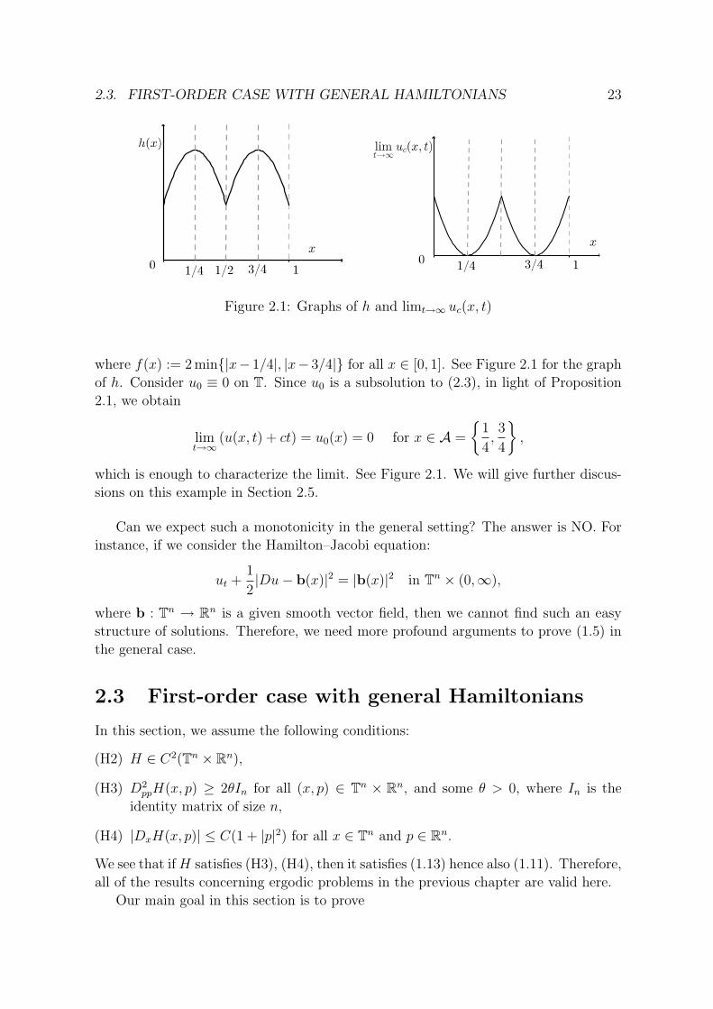
Figure 2.1: Graphs of h and limt→∞ uc(x, t)
where f(x) := 2 min{|x− 1/4|, |x− 3/4|} for all x ∈ [0, 1]. See Figure 2.1 for the graph
of h. Consider u0 ≡ 0 on T. Since u0 is a subsolution to (2.3), in light of Proposition
2.1, we obtain
limt→∞
(u(x, t) + ct) = u0(x) = 0 for x ∈ A =
{1
4,3
4
},
which is enough to characterize the limit. See Figure 2.1. We will give further discus-
sions on this example in Section 2.5.
Can we expect such a monotonicity in the general setting? The answer is NO. For
instance, if we consider the Hamilton–Jacobi equation:
ut +1
2|Du− b(x)|2 = |b(x)|2 in Tn × (0,∞),
where b : Tn → Rn is a given smooth vector field, then we cannot find such an easy
structure of solutions. Therefore, we need more profound arguments to prove (1.5) in
the general case.
2.3 First-order case with general Hamiltonians
In this section, we assume the following conditions:
(H2) H ∈ C2(Tn × Rn),
(H3) D2ppH(x, p) ≥ 2θIn for all (x, p) ∈ Tn × Rn, and some θ > 0, where In is the
identity matrix of size n,
(H4) |DxH(x, p)| ≤ C(1 + |p|2) for all x ∈ Tn and p ∈ Rn.
We see that ifH satisfies (H3), (H4), then it satisfies (1.13) hence also (1.11). Therefore,
all of the results concerning ergodic problems in the previous chapter are valid here.
Our main goal in this section is to prove

24 CHAPTER 2. LARGE TIME ASYMPTOTICS
Theorem 2.2. Assume that (H2)–(H4) hold. Let u be the solution of (1.1) with a
given initial data u0 ∈ Lip (Tn). Then there exists (v, c) ∈ Lip (Tn) × R, a solution of
ergodic problem (1.6), such that (1.5) holds, that is,
u(x, t) − (v(x) − ct) → 0 uniformly for x ∈ Tn.
We call v − ct obtained in Theorem 2.2 the asymptotic solution for (1.1).
Remark 2.1. It is worth pointing out delicate things on the convexity assumption
here. Assumption (H3) is a uniform convexity assumption. We can actually easily
weaken this to a strictly convexity assumption, i.e., D2ppH > 0, since we do have an a
priori estimate on the Lipschitz continuity of solutions. Therefore, we can construct a
uniformly convex Hamilton–Jacobi equation which has the same solution as that of a
strictly convex one.
On the other hand, this “strictness” of convexity is very important to get conver-
gence (1.5). Consider the following explicit example:
ut + |ux − 1| = 1 in R × (0,∞), u(·, 0) = sin(x).
Then, it is clear that
u(x, t) = sin(x+ t) for all (x, t) ∈ R × [0,∞)
is the solution of the above but convergence (1.5) does not hold. This was first pointed
out by Barles and Souganidis in [12].
We also point out that the convexity is NOT a necessary condition either, since it
is known that there are convergence results for possibly nonconvex Hamilton–Jacobi
equations in [12, 8]. A typical example for nonconvex Hamiltonians is H(x, p) :=
(|p|2 − 1)2 − V (x).
2.3.1 Formal calculation
In this subsection, we describe the idea in [17] in a heuristic way to get
ut(·, t) → −c as t→ ∞ in the viscosity sense, (2.7)
where c is the ergodic constant of (1.6). We call this an asymptotic monotone property
of the solution to (1.1). This is a much stronger result than that of Proposition 1.7.
We “assume” that u is smooth below in the derivation. Notice that this is a completely
formal assumption as we cannot expect a global smooth solution u of Hamilton–Jacobi
equations in general.
Let us first fix T > 0. We consider the adjoint equation of the linearized operator
of the Hamilton–Jacobi equation:{−σt − div
(DpH(x,Du(x, t))σ
)= 0 in Tn × (0, T )
σ(x, T ) = δx0(x) on Tn,(2.8)
2.3. FIRST-ORDER CASE WITH GENERAL HAMILTONIANS 25
where δx0 is the Dirac delta measure at a fixed point x0 ∈ Tn. Note that although (2.8)
may have only a very singular solution, we do not mind in this section as this is just a
formal argument. It is clear that
σ(x, t) ≥ 0 and
∫Tn
σ(x, t) dx = 1 for all (x, t) ∈ Tn × [0, T ]. (2.9)
Then, we have the following conservation of energy:
d
dt
∫Tn
H(x,Du(x, t))σ(x, t) dx
=
∫Tn
DpH(x,Du) ·Dutσ dx+
∫Tn
H(x,Du)σt dx
= −∫
Tn
div(DpH(x,Du)σ
)ut dx−
∫Tn
utσt dx = 0,
which implies a new “formula”:
ut(x0, T ) =
∫Tn
ut(·, T )δx0 dx = −∫
Tn
H(x,Du)σ dx∣∣∣t=T
= − 1
T
∫ T
0
∫Tn
H(x,Du)σ dxdt.
Noting (2.9) and |Du(x, t)| ≤ C by Proposition 1.8, in light of the Riesz theorem,
there exists νT ∈ P(Tn × Rn) such that∫∫Tn×Rn
ϕ(x, p) dνT (x, p) =1
T
∫ T
0
∫Tn
ϕ(x,Du)σ dxdt
for all ϕ ∈ Cc(Tn×Rn). Here P(Tn×Rn) is the set of all Radon probability measures on
Tn×Rn. Because of the gradient bound of u, we obtain that supp (νT ) ⊂ Tn×B(0, C),
where supp (νT ) denotes the support of νT , that is,
supp (νT ) ={(x, p) ∈ Tn × Rn : νT
(B((x, p), r)
)> 0 for all r > 0
}.
Since ∫∫Tn×Rn
dνT (x, p) = 1,
there exists a subsequence Tj → ∞ as j → ∞ so that
νTj⇀ ν ∈ P(Tn × Rn) as j → ∞ (2.10)
in the sense of measures. Then, we can expect some important facts
(i) ν is a Mather measure associated with (1.6),
(ii) supp ν ⊂ {(x, p) ∈ Tn × Rn : p = Dv(x)}, where v is a viscosity solution to (1.6).

26 CHAPTER 2. LARGE TIME ASYMPTOTICS
We do not give the proofs of these facts here. We will give the definition of Mather
measures in Chapter 3. Property (ii) in the above is called the graph theorem in the
Hamiltonian dynamics, which is an extremely important result (see [63, 62] for details).
One way to look at (i) is the following: if we think of Du as a given function in (2.8),
then (2.8) is a transport equation, and the characteristic ODE is given by{X(t) = DpH(X(t), Du(X(t), t)
)for t ∈ (0, T )
X(T ) = x0,(2.11)
which is formally equivalent to the Hamiltonian system.
If we admit these, then we obtain
ut(x0, Tj) = − 1
Tj
∫ Tj
0
∫Tn
H(x,Du)σ dxdt
= −∫∫
Tn×Rn
H(x, p) dνTj(x, p) → −
∫∫Tn×Rn
H(x, p) dν(x, p) = −c
as j → ∞ for any subsequence Tj satisfying (2.10).
Now, we should ask ourselves how we can make this argument rigorous. Some
important points are
(i) to introduce a regularizing process for (1.1),
(ii) to introduce a scaling process for t as we need to look at both limits of a regu-
larizing process and the large-time behavior, and
(iii) to give good estimates,
which are discussed in details in the next subsections.
2.3.2 Regularizing process
In the following subsections, we make the formal argument in Section 2.3.1 rigorous by
using a regularizing process and giving important estimates.
We only need to study the case where the ergodic constant c = 0, and we always
assume it henceforth. Indeed, by replacing, if necessary, H and u(x, t) by H − c and
u(x, t) + ct, respectively, we can always reduce the situation to the case that c = 0.
We first consider a rescaled problem. Let u be the solution of (1.1). For ε > 0, set
uε(x, t) = u(x, t/ε) for (x, t) ∈ Tn × [0,∞). Then, uε satisfies
(C)ε
{εuε
t +H(x,Duε) = 0 in Tn × (0,∞),
uε(x, 0) = u0(x) on Tn.
By repeating the proof of Proposition 1.8 with a small modification, we have the
following a priori estimates
‖uεt‖L∞(Tn×[0,1]) ≤ C/ε, ‖Duε‖L∞(Tn×[0,1]) ≤ C. (2.12)

2.3. FIRST-ORDER CASE WITH GENERAL HAMILTONIANS 27
for some constant C > 0 independent of ε. Notice that in general, the function uε is
only Lipschitz continuous.
For this reason, we add a viscosity term to (C)ε, and consider the following regu-
larized equation
(A)ε
{εwε
t +H(x,Dwε) = ε4∆wε in Tn × (0,∞),
wε(x, 0) = u0(x) on Tn.
We also consider a corresponding approximation for the ergodic problem (1.6):
(E)ε H(x,Dvε) = ε4∆vε +Hε in Tn.
By Theorem 1.2 and Proposition 1.4, the existence and uniqueness of the ergodic
constant Hε of (E)ε holds. Besides, there exists a smooth solution vε to (E)ε.
The advantage of considering (A)ε and (E)ε lies in the fact that the solutions of
these equations are smooth, and this will allow us to use the nonlinear adjoint method
to perform rigorous calculations in the next subsection.
Proposition 2.3. Assume that (1.11), (H2) and (H4) hold, and the ergodic constant
of (1.6) is 0. Let uε and wε be the solution of (C)ε and (A)ε with a given initial data
u0 ∈ Lip (Tn), respectively. There exists C > 0 independent of ε such that
‖uε(·, 1) − wε(·, 1)‖L∞(Tn) ≤ Cε,
|Hε| ≤ Cε2.
Proof. We consider the function Φ : Tn × Tn × [0, 1] → R defined by
Φ(x, y, t) := uε(x, t) − wε(y, t) − |x− y|2
2η−Kt
for η > 0 and K > 0 to be fixed later. Pick (xη, yη, tη) ∈ Tn × Tn × [0, 1] such that
Φ(xη, yη, tη) = maxx,y∈Tn, t∈[0,1]
Φ.
In the case tη > 0, in light of Ishii’s lemma (see [23, Theorem 3.2.19]), for any
ρ ∈ (0, 1), there exist (aη, pη, Xη) ∈ J2,+uε(xη, tη) and (bη, pη, Yη) ∈ J
2,−wε(yη, tη) such
that
aη − bη = K, pη =xη − yη
η,
(Xη 0
0 −Yη
)≤ Aη + ρA2
η, (2.13)
where
Aη :=1
η
(In −In−In In
).
Here, J2,±
denotes the super-semijet, and sub-semijet, respectively (see Section 4.2).

28 CHAPTER 2. LARGE TIME ASYMPTOTICS
We need to be careful for the case tη = 1, which is handled by Lemma 4.4. By the
definition of viscosity solutions,
εaη +H(xη, pη) ≤ 0 and εbη +H(xη, pη) ≥ ε4tr (Yη),
which implies
εK +H(xη, pη) −H(yη, pη) ≤ −ε4tr (Yη).
Note that
−ε4tr (Yη) =n∑
i=1
{〈Xη0ei, 0ei〉 − 〈Yηε
2ei, ε2ei〉
}≤
n∑i=1
{Aη
(0ei
ε2ei
)·(
0ei
ε2ei
)+ ρA2
η
(0ei
ε2ei
)·(
0ei
ε2ei
)}≤ Cε4
η+O(ρ).
Since Φ(yη, yη, tη) ≤ Φ(xη, yη, tη), we have
uε(yη, tη) − wε(yη, tη) −Ktη ≤ uε(xη, tη) − wε(yη, tη) −|xη − yη|2
2η−Ktη,
which implies |pη| ≤ C for some C > 0 in view of the Lipschitz continuity of uε. Thus,
|xη − yη| ≤ Cη. Therefore,
|H(xη, pη) −H(yη, pη)| ≤ C(1 + |pη|2)|xη − yη| ≤ Cη.
Combine the above to deduce
εK ≤ Cε4/η + Cη +O(ρ) as ρ→ 0.
Sending ρ→ 0 and setting K := C ′ε−1(ε4/η + η) for C ′ > C, we necessarily have
tη = 0.
Thus, we get, for all x ∈ Tn, t ∈ [0, 1],
Φ(x, x, t) ≤ Φ(xη, yη, tη) = Φ(xη, yη, 0),
which reads for t = 1,
uε(x, 1) − wε(x, 1) ≤ u0(xη) − u0(yη) +K
≤‖Du0‖L∞(Tn)η + C ′ε−1(ε4
η+ η
)= C
(ε3
η+
(1 +
1
ε
)η
).
Setting
η := ε2,

2.3. FIRST-ORDER CASE WITH GENERAL HAMILTONIANS 29
we get uε(x, 1) − wε(x, 1) ≤ Cε2 for all x ∈ Tn. By exchanging the role of uε and wε
in Φ and repeating a similar argument, we obtain ‖uε(·, 1) − wε(·, 1)‖L∞(Tn) ≤ Cε2.
Let us now prove ∣∣Hε
∣∣ =∣∣Hε − c
∣∣ ≤ Cε2
in a similar way. Set
Ψ(x, y) := v(x) − vε(y) − |x− y|2
2η,
where vε and v are solutions to (E)ε and (1.6), respectively. For a maximum point
(xη, yη) of Ψ on Tn × Tn, we have
H(xη, pη) ≤ 0 and H(yη, pη) ≥ ε4tr (Yη) +Hε
for any (pη, Xη) ∈ J2,+v(xη), (pη, Yη) ∈ J
2,−vε(yη). Note here that we are assuming the
ergodic constant of (1.6) is c = 0 now.
Therefore, similarly to the above,
Hε − 0 ≤ H(yη, pη) −H(xη, pη) − ε4tr (Yη) ≤ C
(η +
ε4
η
).
Setting η = ε2, we obtain Hε ≤ Cε2. Symmetrically, we can prove Hε ≥ −Cε2, which
yields the conclusion.
Remark 2.2. As seen in the proof, the vanishing viscosity method gives that the rate
of convergence of uε − wε is√viscosity coefficient/(the coefficient of uε
t and wεt ).
Because of this fact, we can choose εα for any α > 2 as a coefficient of the viscosity
terms in (A)ε and (E)ε. We choose α = 4 here just to make the computations nice and
clear.
2.3.3 Conservation of energy and a key observation
The adjoint equation of the linearized operator of (A)ε is
(AJ)ε
{−εσε
t − div(DpH(x,Dwε)σε) = ε4∆σε in Tn × (0, 1),
σε(x, 1) = δx0 on Tn.
Proposition 2.4 (Elementary Property of σε). Assume that (H2)–(H4) hold. We have
σε > 0 in Tn × (0, 1), and∫Tn
σε(x, t) dx = 1 for all t ∈ [0, 1].
30 CHAPTER 2. LARGE TIME ASYMPTOTICS
Proof. We have that σε > 0 in Tn × (0, 1) by the strong maximum principle for (AJ)ε.
Since
εd
dt
∫Tn
σε(·, t) dx =
∫Tn
(−div(DpH(x,Dwε)σε) − ε4∆σε
)dx = 0,
we conclude ∫Tn
σε(x, t) dx =
∫Tn
σε(x, 1) dx =
∫Tn
δx0 dx = 1
for all t ∈ [0, 1], which is the conclusion.
Lemma 2.5 (Conservation of Energy 1). Assume that (H2)–(H4) hold. Then we have
the following properties
(i)d
dt
∫Tn
(H(x,Dwε) − ε4∆wε)σε dx = 0,
(ii) εwεt (x0, 1) = −
∫ 1
0
∫Tn
(H(x,Dwε) − ε4∆wε)σε dx dt.
Proof. We only need to prove (i) as (ii) follows directly from (i). This is a straightfor-
ward result of adjoint operators and comes from a direct calculation:
d
dt
∫Tn
(H(x,Dwε) − ε4∆wε)σε dx
=
∫Tn
(DpH(x,Dwε) ·Dwεt − ε4∆wε
t )σε dx+
∫Tn
(H(x,Dwε) − ε4∆wε)σεt dx
= −∫
Tn
(div
(DpH(x,Dwε)σε
)+ ε4∆σε
)wε
t dx−∫
Tn
εwεtσ
εt dx = 0.
Remark 2.3.
(i) We stress the fact that identity (ii) in Lemma 2.5 is extremely important. If we
scale back the time, the integral on the right hand side becomes
− 1
T
∫ T
0
∫Tn
[H(x,Dwε) − ε4∆wε
]σε(x, t) dx dt,
where T = 1/ε→ ∞. This is the averaging action as t→ ∞, which is a key observation.
We observed this in a formal calculation in Section 2.3.1.
(ii) We emphasize here that we do not use any specific structure of the equations up
to now, and therefore this conservation law holds in a much more general setting. To
analyze further, we need to require more specific structures and perform some delicate
analysis. But it is worth mentioning that, in this reason, this method for the large-time
asymptotics for nonlinear equations is universal and robust in principle.
The following theorem is a rigorous interpretation of asymptotic monotone property
(2.7) of the solution to (1.1), which is essential in the proof of Theorem 2.2.
Theorem 2.6. Assume that (H2)–(H4) hold, and the ergodic constant of (1.6) is 0.
We have
limε→0
ε‖wεt (·, 1)‖L∞(Tn) = 0.
2.3. FIRST-ORDER CASE WITH GENERAL HAMILTONIANS 31
More precisely, there exists a positive constant C, independent of ε, such that
ε‖wεt (·, 1)‖L∞(Tn) = ‖H(·, Dwε(·, 1)) − ε4∆wε(·, 1)‖L∞(Tn) ≤ Cε1/2.
To prove this, we use the following key estimates, which will be proved in the next
subsection.
Lemma 2.7 (Key Estimates 1). Assume that (H2)–(H4) hold, and the ergodic constant
of (1.6) is 0. There exists a positive constant C, independent of ε, such that the
followings hold:
(i)
∫ 1
0
∫Tn
|D(wε − vε)|2σε dx dt ≤ Cε,
(ii)
∫ 1
0
∫Tn
|D2(wε − vε)|2σε dx dt ≤ Cε−7.
We now give the proof of Theorem 2.6 by using the averaging action above and the
key estimates in Lemma 2.7.
Proof of Theorem 2.6. Let us first choose x0, which may depend on ε, such that
|εwεt (x0, 1)| = ‖εwε
t (·, 1)‖L∞(Tn) = ‖H(·, Dwε(·, 1)) − ε4∆wε(·, 1)‖L∞(Tn).
Thanks to Lemma 2.5,
|εwεt (x0, 1)| =
∣∣∣∣∫ 1
0
∫Tn
(H(x,Dwε) − ε4∆wε)σε dx dt
∣∣∣∣ .Let vε be a solution of (E)ε. By Proposition 2.3,
ε‖wεt (·, 1)‖L∞(Tn)
=
∣∣∣∣∫ 1
0
∫Tn
(H(x,Dwε) − ε4∆wε)σε dx dt
∣∣∣∣=
∣∣∣∣∫ 1
0
∫Tn
(H(x,Dwε) − ε4∆wε − (H(x,Dvε) − ε4∆vε −Hε))σε dx dt
∣∣∣∣≤
∫ 1
0
∫Tn
|H(x,Dwε) −H(x,Dvε)|σε + ε4|∆(wε − vε)|σε dx dt+ |Hε|
≤C
∫ 1
0
∫Tn
[|D(wε − vε)| + ε4|D2(wε − vε)|
]σε dx dt+ Cε2.
We finally use the Holder inequality and Lemma 2.7 to get that
ε‖wεt (·, 1)‖L∞(Tn)
≤C
[(∫ 1
0
∫Tn
|D(wε − vε)|2σε dx dt
)1/2
+ ε4
(∫ 1
0
∫Tn
|D2(wε − vε)|2σε dx dt
)1/2
+ ε2
]≤Cε1/2.

32 CHAPTER 2. LARGE TIME ASYMPTOTICS
Let us now present the proof of the large time asymptotics of u, Theorem 2.2.
Proof of Theorem 2.2. Firstly, the equi-Lipschitz continuity of {wε(·, 1)}ε>0 is obtained
by an argument similar to that of the proof of Theorem 1.2. Therefore, we are able to
choose a sequence εm → 0 as m → ∞ such that {wεm(·, 1)}m∈N converges uniformly
to a continuous function v in Tn, which may depend on the choice of {εm}m∈N. We let
tm := 1/εm for m ∈ N, and use Proposition 2.3 to deduce that
‖u(·, tm) − v‖L∞(Tn) → 0 as m→ ∞.
Let us show that the limit of u(·, t) as t → ∞ does not depend on the sequence
{tm}m∈N. In view of Theorem 2.6, which is one of our main results in this chapter,
v is a solution of (E), and thus a (time independent) solution of the equation in (C).
Therefore, for any x ∈ Tn, and t > 0 such that tm ≤ t < tm+1, we use the comparison
principle for (C) to yield that
|u(x, t) − v(x)| ≤ ‖u(·, tm + (t− tm)) − v(·)‖L∞(Tn) ≤ ‖u(·, tm) − v(·)‖L∞(Tn).
Thus,
limt→∞
‖u(·, t) − v(·)‖L∞(Tn) ≤ limm→∞
‖u(·, tm) − v(·)‖L∞(Tn) = 0,
which gives the conclusion.
2.3.4 Proof of key estimates
A key idea to prove estimates in Lemma 2.7 is to use a combination of the Bernstein
method and the adjoint technique.
Lemma 2.8. Assume that (H2), (H4) hold. Let wε be the solution of (A)ε. There
exists a constant C > 0 independent of ε such that∫ 1
0
∫Tn
ε4|D2wε|2σε dx dt ≤ C.
This is one of the key estimates which was first introduced by Evans [32] in the
study of gradient shock structures of the vanishing viscosity procedure of nonconvex,
first-order Hamilton–Jacobi equations. See also Tran [78]. The convexity of H is not
needed at all to get the conclusion of this lemma as can be seen in the proof.
Proof. By a computation similar to that in the proof of Theorem 1.2, for ϕ(x, t) :=
|Dwε|2/2, we have
εϕt +DpH ·Dϕ+DxH ·Dwε = ε4(∆ϕ− |D2wε|2).
Multiply the above by σε and integrate over Tn × [0, 1] to yield
ε4
∫ 1
0
∫Tn
|D2wε|2σε dxdt = −∫ 1
0
∫Tn
(εϕt +DpH ·Dϕ− ε4∆ϕ
)σε dxdt
−∫ 1
0
∫Tn
DxH ·Dwεσε dxdt.
2.3. FIRST-ORDER CASE WITH GENERAL HAMILTONIANS 33
Integrating by parts, we get∫ 1
0
∫Tn
(εϕt +DpH ·Dϕ− ε4∆ϕ
)σε dxdt
=
∫Tn
[εϕσε]t=1t=0 dx+
∫ 1
0
∫Tn
(−εσε
t − div (DpHσε) − ε4∆σε
)ϕdxdt
≤Cε.
Noting that |DxH ·Dwε| ≤ C, we get the conclusion.
Proof of Lemma 2.7 (i). Subtracting equation (A)ε from (E)ε, thanks to the uniform
convexity of H, we get
0 = ε(vε − wε)t +H(x,Dvε) −H(x,Dwε) − ε4∆(vε − wε) −Hε
≥ ε(vε − wε)t +DpH(x,Dwε) ·D(vε − wε) + θ|D(vε − wε)|2 − ε4∆(vε − wε) −Hε.
Multiply the above inequality by σε and integrate by parts on Tn × [0, 1] to deduce
that
θ
∫ 1
0
∫Tn
|D(wε − vε)|2σε dx dt
≤Hε −∫ 1
0
∫Tn
ε((vε − wε)σε)t dxdt
+
∫ 1
0
∫Tn
[εσε
t + div (DpH(x,Dwε)σε) + ε4∆σε](vε − wε) dxdt
=Hε + ε
[∫Tn
(wε − vε)σε dx
]t=1
t=0
=Hε + ε(wε(x0, 1) − vε(x0)) − ε
∫Tn
(u0(x) − vε(x))σε(x, 0) dx
=Hε + εwε(x0, 1) − ε
∫Tn
(vε(x0) − vε(x))σε(x, 0) dx− ε
∫Tn
u0(x)σε(x, 0) dx.
Note here that wε satisfies∥∥∥∥wε +Hεt
ε
∥∥∥∥L∞(Tn×(0,∞))
≤ C for some C > 0,
as we see in the proof of Proposition 1.6. Thus, Hε + εwε(x0, 1) ≤ Cε and
θ
∫ 1
0
∫Tn
|D(wε − vε)|2σε dx dt ≤ ε(C + ‖Dvε‖L∞(Tn) + ‖u0‖L∞(Tn)) ≤ Cε,
which implies the conclusion.

34 CHAPTER 2. LARGE TIME ASYMPTOTICS
Proof of Lemma 2.7 (ii). Subtract (A)ε from (E)ε and differentiate with respect to xi
to get
ε(vε − wε)xit +DpH(x,Dvε) ·Dvεxi−DpH(x,Dwε) ·Dwε
xi
+Hxi(x,Dvε) −Hxi
(x,Dwε) − ε4∆(vε − wε)xi= 0.
Let ϕ(x, t) := |D(vε−wε)|2/2. Multiplying the last identity by (vε−wε)xiand summing
up with respect to i, we achieve that
εϕt +DpH(x,Dwε) ·Dϕ+[(DpH(x,Dvε) −DpH(x,Dwε)
)·Dvε
xi
](vε
xi− wε
xi)
+(DxH(x,Dvε) −DxH(x,Dwε)
)·D(vε − wε) − ε4
(∆ϕ− |D2(vε − wε)|2
)= 0.
By using the equi-Lipschitz continuity of vε, wε and (H4), we derive that
εϕt +DpH(x,Dwε) ·Dϕ− ε4∆ϕ+ ε4|D2(vε − wε)|2
≤C(|D2vε| + 1)|D(vε − wε)|2. (2.14)
The right hand side of (2.14) is a dangerous term because of the term |D2vε|. We now
take advantage of Lemma 2.8 to handle it. Using the fact that ‖Dvε‖L∞ and ‖Dwε‖L∞
are bounded, we have
C|D2vε| |D(vε − wε)|2 ≤ C|D2(vε − wε)| |D(vε − wε)|2 + C|D2wε| |D(vε − wε)|2
≤ ε4
2|D2(vε − wε)|2 +
C
ε4|D(vε − wε)|2 + C|D2wε|. (2.15)
Combine (2.14) and (2.15) to deduce
εϕt +DpH(x,Dwε) ·Dϕ− ε4∆ϕ+ε4
2|D2(vε − wε)|2
≤ C|D(vε − wε)|2 +C
ε4|D(vε − wε)|2 + C|D2wε|. (2.16)
We multiply (2.16) by σε, integrate over Tn × [0, 1], and use integration by parts to
yield that, in light of Lemma 2.8 and (i),
ε4
∫ 1
0
∫Tn
|D2(wε − vε)|2σε dx dt ≤ Cε+C
ε4ε+ C
∫ 1
0
∫Tn
|D2wε|σε dx dt
≤ C
ε3+ C
(∫ 1
0
∫Tn
|D2wε|2σε dx dt)1/2(∫ 1
0
∫Tn
σε dx dt)1/2
≤ C
ε3+C
ε2≤ C
ε3.
Remark 2.4. The estimates in Lemma 2.7 give us much better control of D(wε − vε)
and D2(wε−vε) on the support of σε. More precisely, the classical a priori estimates by
using the Bernstein method as in the proof of Theorem 1.2 only imply that D(wε − vε)
and ε4∆(wε − vε) are bounded.

2.4. DEGENERATE VISCOUS CASE 35
By using the adjoint equation, we can get further formally that ε−1/2D(wε − vε)
and ε7/2D2(wε−vε) are bounded on the support of σε. Clearly, these new estimates are
much stronger than the known ones on the support of σε. However, we must point out
that, as ε→ 0, the supports of subsequential limits of {σε}ε>0 could be very singular.
Understanding deeper about this point is essential in achieving further developments
of this new approach in the near future.
It is also worth mentioning that we eventually do not need to use the graph theorem
in the whole procedure above.
2.4 Degenerate viscous case
In this section, we consider a general possibly degenerate viscous Hamilton–Jacobi
equation:
ut − tr(A(x)D2u
)+H(x,Du) = 0 in Tn × (0,∞). (2.17)
Here is one of the main results of [17].
Theorem 2.9. Assume that (H1)–(H4) hold. Let u be the solution of (2.17) with initial
data u(·, 0) = u0 ∈ Lip (Tn). Then there exists (v, c) ∈ Lip (Tn) × R such that (1.5)
holds, that is,
u(x, t) − (v(x) − ct) → 0 uniformly for x ∈ Tn as t→ ∞,
where the pair (v, c) is a solution of the ergodic problem
−tr(A(x)D2v
)+H(x,Dv) = c in Tn.
For an easy explanation, we consider the 1-dimensional case (i.e., n = 1) in this
section. This makes the problem much easier but we do not lose the key difficulties
coming from the degenerate viscous term −tr(A(x)D2u
). We now assume that the
ergodic constant c for (1.8) is 0 as in Section 2.3.3.
We repeat the same procedures as those in Sections 2.3.2 and 2.3.3. Associated
problems are now described below:
(C) ut − a(x)uxx +H(x, ux) = 0 in T × (0,∞), u(x, 0) = u0(x) in T,(A)ε εwε
t − a(x)wεxx +H(x,wε
x) = ε4wεxx in T × (0,∞), wε(x, 0) = u0(x) in T,
(AJ)ε − εσεt − (a(x)σε)xx − (Hp(x,w
εx)σ
ε)x = ε4σεxx in T × (0, 1), σε(x, 1) = δx0 in T,
(E)ε − a(x)vεxx +H(x, vε
x) = ε4vεxx +Hε in T.
Here, assumption (H1) means that a ∈ C2(T) is a nonnegative function.
As pointed out in Remark 2.3, we have the same type conservation of energy.
Lemma 2.10 (Conservation of Energy 2). Assume that (H1)–(H4) hold, and the as-
sociated ergodic constant is zero. The following properties hold:
(i)d
dt
∫T
[H(x,wε
x) − (a(x) + ε4)wεxx
]σε dx = 0,
(ii) εwεt (x0, 1) = −
∫ 1
0
∫T
[H(x,wε
x) − (a(x) + ε4)wεxx
]σε dx dt.
36 CHAPTER 2. LARGE TIME ASYMPTOTICS
The proof of this lemma is similar to that of Lemma 2.5, hence is omitted.
Now, as in the proof of Theorem 2.6, we have
ε‖wεt (·, 1)‖L∞(T) = ‖H(·, wε
x(·, 1)) − (ε4 + a(x))wεxx(·, 1)‖L∞(T)
=
∣∣∣∣∫ 1
0
∫T
[H(x,wε
x) − (ε4 + a(x))wεxx
]σε dx dt
∣∣∣∣=
∣∣∣∣∫ 1
0
∫T
[H(x,wε
x) − (ε4 + a(x))wεxx − (H(x, vε
x) − (ε4 + a(x))vεxx −Hε)
]σε dx dt
∣∣∣∣≤
∫ 1
0
∫T
(|H(x,wε
x) −H(x, vεx)| + |(ε4 + a(x))(wε − vε)xx|
)σε dx dt+
∣∣Hε
∣∣≤C
[ (∫ 1
0
∫T|(wε − vε)x|2σε dx dt
)1/2
+ ε4
(∫ 1
0
∫T|(wε − vε)xx|2σε dx dt
)1/2
+
(∫ 1
0
∫Ta(x)2|(wε − vε)xx|2σε dx dt
)1/2
+∣∣Hε
∣∣ ],
where vε is a solution of (E)ε (vε is unique up to an additive constant).
Since c = 0, we have∣∣Hε
∣∣ ≤ Cε2. Therefore, in order to control ε‖wεt (·, 1)‖L∞(T),
we basically need to bound three terms on the right hand side of the above. The first
two already appear in the previous section, and the last term is a new term due to the
appearance of the possibly degenerate diffusion a(x). We now redo the same procedure
to handle these three with great care as the possibly degenerate diffusion a(x) is quite
dangerous.
Lemma 2.11 (Key Estimates 2). Assume that (H1)–(H4) hold, and the associated
ergodic constant is zero. There exists a constant C > 0, independent of ε, such that
(i)
∫ 1
0
∫T|(wε − vε)x|2σε dx dt ≤ Cε,
(ii)
∫ 1
0
∫T(a(x) + ε4)|wε
xx|2σε dx dt ≤ C,
(iii)
∫ 1
0
∫T|(wε − vε)xx|2σε dx dt ≤ Cε−7,
(iv)
∫ 1
0
∫Ta2(x)|(wε − vε)xx|2σε dx dt ≤ C
√ε.
Proof. The proof of (i) is similar to that of Lemma 2.7 (i), hence is omitted. Notice that
if we do not differentiate the equation, then we do not have any difficulty which comes
from the diffusion term a(x). On the other hand, once we differentiate the equation
to obtain some estimates, then we face some of difficulties coming from the term a as
seen below.
We now prove (ii). Let wε be the solution of (A)ε. Differentiate (A)ε with respect
to the x variable to get
εwεtx +Hp(x,w
εx) · wε
xx +Hx(x,wεx) − (ε4 + a)wε
xxx − axwεxx = 0. (2.18)

2.4. DEGENERATE VISCOUS CASE 37
Here we write Hp(x, p) = DpH(x, p), Hx(x, p) = DxH(x, p) as we are in the 1-
dimensional space.
Let ξ(x, t) := |wεx|2/2. Note that
ξt = wεxw
εxt, ξx = wε
xwεxx, ξxx = |wε
xx|2 + wεxw
εxxx.
Multiply (2.18) by wεx to arrive at
εξt +Hp · ξx +Hx · wεx = (ε4 + a)(ξxx − |wε
xx|2) + (ax · wεx)w
εxx.
We need to be careful for the last term which comes from the diffusion term. Notice
first that we have
a2x(x) ≤ Ca(x) for all x ∈ T (2.19)
since a ∈ C2(T). Indeed, a ∈ C2(T) implies√a ∈ Lip (T). Thus, |ax| = |2(
√a)x
√a| ≤
C√a. We next notice that for δ > 0 small enough,
axwεxw
εxx ≤ C|ax||wε
xx| ≤C
δ+ δa2
x|wεxx|2 ≤ C +
1
2a|wε
xx|2. (2.20)
Hence,
εξt +Hp · ξx − (ε4 + a)ξxx + (ε4 +a
2)|wε
xx|2 ≤ C.
Multiply the above by σε, integrate over T× [0, 1], and use integration by parts to yield
the conclusion of (ii).
Next, we prove (iii). Subtract (A)ε from (E)ε and differentiate with respect to the
variable x to get
ε(vε − wε)xt +Hp(x, vεx) · vε
xx −Hp(x,wεx) · wε
xx
+Hx(x, vεx) −Hx(x,w
εx) − (ε4 + a)(vε − wε)xxx − ax(v
ε − wε)xx = 0.
Let ϕ(x, t) := |(vε − wε)x|2/2. Multiplying the last identity by (vε − wε)x, we achieve
that
εϕt +Hp(x,wεx) · ϕx +
[(Hp(x, v
εx) −Hp(x,w
εx)
)· vε
xx
](vε − wε)x
+(Hx(x, v
εx) −Hx(x,w
εx)
)· (vε − wε)x + (ε4 + a(x))(|(vε − wε)xx|2 − ϕxx)
− [ax · (vε − wε)xx] (vε − wε)x = 0.
We only need to be careful for the last term as in the above
∣∣[ax · (vε − wε)xx
](vε − wε)x
∣∣ ≤ δ|ax|2|(vε − wε)xx|2 +1
δ|(vε − wε)x|2
≤ a
2|(vε − wε)xx|2 + C|(vε − wε)x|2

38 CHAPTER 2. LARGE TIME ASYMPTOTICS
for δ > 0 small enough. Thus,
εϕt +Hp(x,wεx) · ϕx − (ε4 + a(x))ϕxx +
(ε4 +
a
2
)|(vε − wε)xx|2
≤ C(1 + |vεxx|)|(vε − wε)x|2. (2.21)
By using the same trick as (2.15), we get
εϕt +Hp(x,wεx) · ϕx − (ε4 + a(x))ϕxx +
(ε4
2+a
2
)|(vε − wε)xx|2
≤ C|(vε − wε)x|2 +C
ε4|(vε − wε)x|2 + C|wε
xx|.
We multiply the above by σε, integrate over T× [0, 1], and use integration by parts to
yield that∫ 1
0
∫T(ε4 + a(x))|(wε − vε)xx|2σε dx dt ≤ Cε+
C
ε4ε+ C
∫ 1
0
∫T|wε
xx|σε dx dt
≤ C
ε3+ C
(∫ 1
0
∫T|wε
xx|2σε dx dt)1/2(∫ 1
0
∫Tσε dx dt
)1/2
≤ C
ε3+C
ε2≤ C
ε3,
which implies the conclusion of (iii).
Finally we prove (iv). Setting
ψ(x, t) := a(x)ϕ(x, t) =a(x)|(vε − wε)x(x, t)|2
2,
and multiplying (2.21) by a(x), we get
εψt +Hp(x,wεx) · (ψx − axϕ) − (ε4 + a(x))(ψxx − axxϕ− 2ax · ϕx)
+ a(x)
(ε4 +
a(x)
2
)|(vε − wε)xx|2 ≤ Ca(x)(|vε
xx| + 1)|(vε − wε)x|2.
Note that ax, axx are bounded. Then,
εψt +Hp(x,wεx) · ψx − (ε4 + a(x))ψxx + a(x)
(ε4 +
a(x)
2
)|(vε − wε)xx|2
≤ Cϕ(x) − 2(ε4 + a(x))ax · ϕx + Ca(x)|vεxx| |(vε − wε)x|2.
For δ > 0 small enough
2|(ε4 + a(x))ax · ϕx| ≤ C(ε4 + a(x))|ax| |(vε − wε)xx| |(vε − wε)x|
≤ δ(ε4 + a(x))|ax|2|(vε − wε)xx|2 +C
δ|(vε − wε)x|2
≤ 1
8(ε4 + a(x))a(x)|(vε − wε)xx|2 + C|(vε − wε)x|2

2.5. ASYMPTOTIC PROFILE OF THE FIRST-ORDER CASE 39
by using (2.19) again. Moreover,
a(x)|vεxx| |(vε − wε)x|2
≤ a(x)|wεxx| |(vε − wε)x|2 + a(x)|(vε − wε)xx| |(vε − wε)x|2
≤ ε1/2a(x)|wεxx|2 +
C
ε1/2|(vε − wε)x|2 +
a(x)2
8|(vε − wε)xx|2 + C|(vε − wε)x|2.
Combining everything, we obtain
εψt +Hp(x,wεx) · ψx − (ε4 + a(x))ψxx +
a(x)2
4|(vε − wε)xx|2
≤ (C + Cε−1/2)|(vε − wε)x|2 + ε1/2a(x)|wεxx|2.
We multiply the above inequality by σε, integrate over T × [0, 1] and use (i), (ii) to
yield (iv).
Thanks to Lemmas 2.10, 2.11, we obtain
Theorem 2.12. Assume that (H1)–(H4) hold, and the associated ergodic constant is
zero. Let wε be the solution of (A)ε with initial data u(·, 0) = u0 ∈ Lip (T). Then,
ε‖wεt (·, 1)‖L∞(T) ≤ Cε1/4 for some C > 0,
Theorem 2.9 in the case n = 1 is a straightforward result of Theorem 2.12 as seen in
the proof of Theorem 2.2. We refer to [17] and [70] for the multi-dimensional setting.
Remark 2.5. If the equation in (C) is uniformly parabolic, that is, a(x) > 0 for all
x ∈ T, then estimate (iii) in Lemma 2.11 is not needed anymore as estimate (iv) in
Lemma 2.11 is much stronger.
On the other hand, if a is degenerate, then (iv) in Lemma 2.11 only provides the
estimate of |D2(wε − vε)|2σε on the support of a, and it is hence essential to use (iii)
in Lemma 2.11 to control the part where a = 0.
2.5 Asymptotic profile of the first-order case
In this section, we investigate the first-order Hamilton–Jacobi equation (1.1) again,
and specifically focus on the asymptotic profile, which is
u∞c [u0](x) := limt→∞
(u(x, t) + ct) ,
where u is the solution to (1.1) and c is the ergodic constant of (1.6). Due to Theorem
2.2, this limit exists. As we have already emphasized many times, because of the
multiplicity of solutions to (1.6), the asymptotic profile v in Theorem 2.2 is completely
decided through the initial data for H fixed. In this section, we try to make clear how
the asymptotic profile depends on the initial data, which is based on the argument by
Davini, Siconolfi [25]. We use the following assumption

40 CHAPTER 2. LARGE TIME ASYMPTOTICS
(H3)’ H : Tn × Rn → R such that lim|p|→∞
H(x, p)
|p|= +∞ uniformly for x ∈ Tn,
D2ppH(x, p) ≥ 0 for all (x, p) ∈ Tn × Rn,
which is weaker than (H3).
Let L : Tn × Rn → R be the Legendre transform of H, that is,
L(x, v) = supp∈Rn
(p · v −H(x, p)) for all (x, v) ∈ Tn × Rn.
The function L is called the Lagrangian in the literature.
We first introduce the notion of the Aubry set.
Definition 2.1. Let c be the ergodic constant of (1.6) and set Lc(x, v) := L(x, v)+c for
any (x, v) ∈ Tn × Rn. We call y ∈ Tn the element of the Aubry set A if the following
inf
{∫ t
0
Lc(γ(s),−γ(s)) ds : t ≥ δ, γ ∈ AC ([0, t],Tn), γ(0) = γ(t) = y
}= 0 (2.22)
is satisfied for any fixed δ > 0.
Let us define the function dc : Tn × Tn → R by
dc(x, y)
:= inf
{∫ t
0
Lc(γ(s),−γ(s)) ds : t > 0, γ ∈ AC ([0, t],Tn), γ(0) = x, γ(t) = y
}.
(2.23)
The function dc plays a role of a fundamental solution for Hamilton–Jacobi equations.
We gather some basic properties of the function dc.
Proposition 2.13. Assume that (H3)’ holds. We have
(i) dc(x, y) = sup{v(x) − v(y) : v is a subsolution of (1.6)},(ii) dc(x, x) = 0 and dc(x, y) ≤ dc(x, z) + dc(z, y) for any x, y, z ∈ Tn,
(iii) dc(·, y) is a subsolution of (1.6) for all y ∈ Tn and a solution of (1.6) in Tn \ {y}for all y ∈ Tn.
Proof. We first prove
v(x) − v(y) ≤∫ t
0
Lc(γ,−γ) ds
for all x, y ∈ Tn, any subsolution v of (1.6), and γ ∈ AC ([0, t],Tn) with γ(0) = x and
γ(t) = y. This is at least formally easy to prove. Indeed, let v be a smooth subsolution
of (1.6). We have the following simple computations
v(x) − v(y) = −∫ t
0
dv(γ(s))
dsds =
∫ t
0
Dv(γ(s)) · (−γ(s)) ds
≤∫ t
0
(L(γ(s),−γ(s)) + c) + (H(γ(s), Dv(γ(s))) − c) ds ≤∫ t
0
Lc(γ(s),−γ(s)) ds.
2.5. ASYMPTOTIC PROFILE OF THE FIRST-ORDER CASE 41
This immediately implies (i). Due to the convexity assumption on H, we can obtain an
approximated smooth subsolution by using mollification as in the proof of Proposition
1.5. By using this approximation, we can make this argument rigorous. We ask the
interested readers to fulfill the details here.
It is straightforward to check that (i) implies (ii), and (iii) is a consequence of (i)
and stability results of viscosity solutions (see Proposition 4.10 in Section 4.5) .
Remark 2.6. We can easily check that y is in A if and only if (2.22) holds only for
some δ0 > 0. Indeed, for any δ > 0, we only need to consider the case where δ > δ0.
Fix ε > 0 and then there exist tε ≥ δ0 and γε ∈ AC ([0, tε],Tn) with γ(0) = γ(tε) = y
such that
0 = v(γε(0)) − v(γε(tε)) ≤∫ tε
0
Lc(γε(s),−γε(s)) ds < ε.
We choose m ∈ N such that mtε ≥ δ and set
γm(s) := γ(s− (j − 1)tε) for s ∈ [(j − 1)tε, jtε], j = 1, . . . ,m.
Then γm(0) = γm(mtε) = y. We calculate that
0 ≤∫ mtε
0
Lc(γm(s),−γm(s)) ds =m∑
j=1
∫ jtε
(j−1)tε
Lc(γ(s− (j − 1)tε),−γ(s− (j − 1)tε)) ds
=m
∫ tε
0
Lc(γ(s),−γ(s)) ds < mε.
Sending ε→ 0 yields
inf
{∫ t
0
Lc(γ(s),−γ(s)) ds : t ≥ δ, γ ∈ AC ([0, t],Tn), γ(0) = γ(t) = y
}= 0
for any δ > 0.
Fathi and Siconolfi in [35] gave a beautiful characterization of the Aubry set as
follows.
Theorem 2.14. Assume that (H3)’ holds. A point y ∈ Tn is in the Aubry set A if and
only if dc(·, y) is a solution of (1.6).
We refer to [35, Proposition 5.8] and [49, Proposition A.3] for the proofs.
Theorem 2.15. Assume that (H3)’ holds. Then the Aubry set A is nonempty, com-
pact, and a uniqueness set of (1.6), that is, if v and w are solutions of (1.6), and v = w
on A, then v = w on Tn.
Proof. Let us first proceed to prove that A is a uniqueness set of (1.6). It is enough to
show that if v ≤ w on A, then v ≤ w on Tn. For any small ε > 0, there exists an open
set Uε such that A ⊂ Uε with ∩ε>0Uε = A, and v ≤ w + ε in Uε. Set Kε := Tn \ Uε.
Fix any z ∈ Kε. Since z 6∈ A, dc(·, z) is not a supersolution at x = z in light of

42 CHAPTER 2. LARGE TIME ASYMPTOTICS
Proposition 2.13 (iii) and Theorem 2.14. Then, there exist a constant rz > 0 and a
function ϕz ∈ C1(Tn) such that B(z, rz) ⊂ Tn \ A,
H(x,Dϕz(x)) < 0 for all x ∈ B(z, rz),
ϕz(z) > 0 = dc(z, z), and ϕz(x) < dc(x, z) for all x ∈ Tn \B(z, rz).
See the proof of Theorem 4.19 for details. We set ψz(x) = max{dc(x, z), ϕz(x)} for
x ∈ Tn and observe that ψz is a subsolution of (1.6) in light of Proposition 4.10, and
that H(x,Dψz(x)) < 0 in a neighborhood Vz of z in the classical sense.
By the compactness of Kε, there is a finite sequence of points {zj}Jj=1 such that
Kε ⊂∪J
j=1 Vzj. We define the function ψ ∈ C(Tn) by ψ(x) = (1/J)
∑Jj=1 ψzj
(x) and
observe by convexity (H3)’ that ψ is a strict subsolution to (1.6) for some neighborhood
V of Kε. Regularizing ψ by mollification, if necessary, we may assume that ψ ∈ C1(V ).
Thus, we may apply the comparison result (see Theorem 4.8 in Section 4.4) to conclude
that v ≤ w + ε in Kε. Sending ε → 0 yields v ≤ w in Tn \ A, which implies the
conclusion.
To prove that A 6= ∅, suppose that for all y ∈ Tn, dc(·, y) is not a solution to
(1.6). By the above argument, for each z ∈ Tn, ψz is a subsolution of (1.6), and
H(x,Dψz(x)) < 0 in a neighborhood Vz of z in the classical sense. By the compactness
of Tn, there is a finite sequence {yi}Ni=1 ⊂ Tn such that Tn =
∪Ni=1 Vyi
. We set w(x) :=
(1/N)∑N
i=1 ψyi(x) for all x ∈ Tn and δ := (1/N) mini=1,...,N δi. By the convexity of
H(x, ·), we have H(x,Dw(x)) ≤ c − δ in Tn in the viscosity sense, which contradicts
the first formula of c in Proposition 1.5.
The compactness of A is a straightforward result of stability of viscosity solutions
(see Proposition 4.9 in Section 4.5).
Theorem 2.16. Assume that (H2)–(H4) hold. Let u∞c [u0] − ct be the asymptotic so-
lution for (1.1), that is, u∞c [u0](x) := limt→∞(u(x, t) + ct), where u is the solution to
(1.1). Then we have, for all y ∈ A,
u∞c [u0](y) = min {dc(y, z) + u0(z) : z ∈ Tn} (2.24)
= sup {v(y) : v is a subsolution to (1.6) with v ≤ u0 in Tn} .
Proof. We write vu0 for the right hand side of (2.24). Let y ∈ A and choose zy ∈ Tn
so that
vu0(y) = dc(y, zy) + u0(zy).
By the definition of the function dc, for any ε > 0, there exists tε > 0 and a curve
ξε ∈ AC ([0, tε],Tn) with ξε(0) = y, ξε(tε) = zy such that
dc(y, zy) >
∫ tε
0
Lc(ξε,−ξε) ds− ε.
By the definition of the Aubry set, for any n ∈ N, there exists a sequence tn ≥ n and
a curve δε ∈ AC ([0, tn],Tn) such that δε(0) = δε(tn) = y, and∫ tn
0
Lc(δε(s),−δε(s)) ds < ε.

2.5. ASYMPTOTIC PROFILE OF THE FIRST-ORDER CASE 43
Define γε ∈ AC ([0, tn + tε],Tn) by
γε(s) =
{δε(s) for s ∈ [0, tn],
ξε(s− tn) for s ∈ [tn, tn + tε].
Note that γε(0) = y and γε(tn + tε) = zy.
!
!
!
!
! "
!" !
!
Figure 2.2
We observe that
vu0(y) >
∫ tε
0
Lc(ξε,−ξε) ds+ u0(zy) − ε
>
∫ tn
0
Lc(δε(s),−δε(s)) ds+
∫ tε
0
Lc(ξε,−ξε) ds+ u0(zy) − 2ε
=
∫ tn+tε
0
Lc(γε,−γε) ds+ u0(zy) − 2ε
≥ uc(y, tn + tε) − 2ε,
where uc(x, t) := u(x, t) + ct for (x, t) ∈ Tn × [0,∞). Thus, sending n→ ∞ and ε→ 0
in this order yields vu0(y) ≥ u∞c (y).
By the definition of vu0 , we can easily check vu0 ≤ u0 on Tn in view of Proposition
2.13 (ii). Note that vu0 is a subsolution to (1.6) in view of Proposition 2.13 (iii)
and Corollary 4.16 (i). Thus, in light of the comparison principle for (1.1), we get
vu0(x)− ct ≤ u(x, t) for all (x, t) ∈ Tn × [0,∞). Thus, vu0(x) ≤ limt→∞(u(x, t) + ct) =
u∞c (x).
The second equality is a straightforward result of Proposition (2.13) with the ob-
servation vu0 ≤ u0 on Tn.
In light of Proposition 2.13, Theorems 2.14, 2.15 and 2.16, we get the following
representation formula for the asymptotic profile:
Corollary 2.17. Assume that (H2)–(H4) holds. Let u∞c [u0] − ct be the asymptotic
solution for (1.1). Then we have the representation formula for the asymptotic profile

44 CHAPTER 2. LARGE TIME ASYMPTOTICS
u∞c [u0] as
u∞c [u0](x) = min {dc(x, y) + vu0(y) : y ∈ A} (2.25)
= inf{v(x) : v is a solution to (1.6) with v ≥ vu0 in Tn},
where
vu0(x) = min{dc(x, z) + u0(z) : z ∈ Tn} for all x ∈ Tn.
Proof. We denote by wu0 the right hand side in (2.25). Note first that this is a solution
of (1.6) in view of Theorem 2.14 and Corollary 4.16. Moreover, we can check that
wu0(x) = min{dc(x, y) + vu0(y) : y ∈ A} = vu0(x) for all x ∈ A
by Proposition 2.13 (i), (ii). Thus, u∞c [u0] ≡ vu0 on A.
In light of a property of a uniqueness set of A, Theorem 2.15, we obtain u∞c [u0] ≡ vu0
on Tn, which is the conclusion.
Example 2.2. Now, let us consider the asymptotic profile for the Hamilton–Jacobi
equation appearing in Example 4.1. As we observe in the beginning of Section 2.2, the
associated ergodic problem is
|Dv| =
√c2 − h(x)2
h(x)2in Tn,
where
c := maxx∈Tn
h(x).
We can easily check that we have the explicit formula for the Aubry set
A := {x ∈ Tn : h(x) = maxTn
h}
from the definition of the Aubry set. Also, we have
dc(x, y) = inf
{∫ t
0
√c2
h(γ(s))2− 1 ds : t > 0, |γ| ≤ 1, γ(0) = x, γ(t) = y
}.
From this, we somehow have a better understanding on how the asymptotic profile
depends on the force term h and the initial data u0 through Corollary 2.17.
Example 2.3. We consider Example 2.2 in a more explicit setting which we discussed
in Example 2.1. Let n = 1 and h be the function given by (2.6). Our goal is to derive
the asymptotic profiles by using the formula given in Corollary 2.17 for some given
initial data u0.
In this setting, we have A = {1/4, 3/4}. Thus, letting u∞c [u0] := limt→∞(u(x, t) +
ct), we obtain by Corollary 2.17,
u∞c [u0](x) = min
{dc
(x,
1
4
)+ vu0
(1
4
), dc
(x,
3
4
)+ vu0
(3
4
)}.

2.5. ASYMPTOTIC PROFILE OF THE FIRST-ORDER CASE 45
We are able to compute dc(·, 1/4), dc(·, 3/4) explicitly as
dc
(x,
1
4
)=
(x− 1
4
)2
for 0 ≤ x ≤ 1
2,
−(x− 3
4
)2
+1
8for
1
2≤ x ≤ 1,
dc
(x,
3
4
)=
−
(x− 1
4
)2
+1
8for 0 ≤ x ≤ 1
2,(
x− 3
4
)2
for1
2≤ x ≤ 1.
Firstly, let u0 = u10 ≡ 0 as in Example 2.1. Then, we can check that vu1
0(x) ≡ 0.
Thus, we conclude that u∞c [u10] coincides with the one which we got in Example 2.1.
Next, let us consider another case where u0 = u20 and u2
0 : R → R is 1-periodic,
u20(x) =
−2
(x− 1
4
)2
+1
8for 0 ≤ x ≤ 1
2,
0 for1
2≤ x ≤ 1.
Notice that u20 is not a subsolution to (2.3). Thus, Proposition 2.1 does not hold.
In this case, we need to find vu20. In this setting, it is not hard to see that
vu20(x) =
−
(x− 1
4
)2
+1
16for 0 ≤ x ≤ 1
2,
0 for1
2≤ x ≤ 1.
Thus, we derive that
u∞c [u20](x) = min
{dc
(x,
1
4
)+
1
16, dc
(x,
3
4
)}.
Figure 2.3: Graph of u∞c [u20]
.

46 CHAPTER 2. LARGE TIME ASYMPTOTICS
2.6 Viscous case
In this subsection, we give a proof of the convergence result (1.5) for (1.2) based on
the strong maximum principle, which is rather simple. It is worth emphasizing that
this argument works only for uniformly parabolic equations including (1.2).
Theorem 2.18. Assume that H ∈ C2(Tn × Rn), (1.11) holds and u0 ∈ C2(Tn). Let u
be the solution of (1.2). Then there exists a solution (v, c) ∈ C2(Tn) × R of (1.7) such
that, as t→ ∞,
u(x, t) − (v(x) − ct) → 0 uniformly on Tn.
The following proof is based on the argument in [13].
Proof. We normalize the ergodic constant c to be 0 as usual.
Let v be a solution of (1.7). By the maximum principle we see that
m(t) := maxx∈Tn
(u(x, t) − v(x))
is nonincreasing. Therefore we have m(t) → m ∈ R as t→ ∞. By the global Lipschitz
regularity result, Proposition 1.8, there exists a sequence {tj}j∈N with tj → ∞ such
that
u(x, t+ tj) → u∞(x, t) locally uniformly on Tn × [0,∞)
as j → ∞ for some u∞ ∈ Lip (Tn × [0,∞)) which may depend on the subsequence
{tj}j∈N at this moment. By a standard stability result of viscosity solutions we see that
u∞ is a solution to the equation in (1.1). Noting thatm(t+tj) = maxx∈Tn (u(x, t+ tj) − v(x)),
we obtain
m = maxx∈Tn
(u∞(x, t) − v(x)) for all t ≥ 0.
By Proposition 2.19 (the strong maximum principle) below, we obtain
m = u∞(x, t) − v(x) for all (x, t) ∈ Tn × [0,∞),
which implies that u∞(x, t) ≡ u∞(x) = v(x) + m. As the right hand side above does
not depend on the choice of subsequences anymore, we see that
u(x, t) → v(x) +m uniformly on Tn as t→ ∞.
Proposition 2.19 (Strong maximum principle). Let U be a bounded domain in Tn
and set UT := U × (0, T ] for each time T > 0. Let u, v be a smooth subsolution and a
smooth supersolution to (1.2), respectively. If, for some given T > 0, u− v attains its
maximum over UT at a point (x0, t0) ∈ UT , then
u− v is constant on Ut0.
See [31] for instance. If we do not have the regularity (smoothness) for solutions,
then we need to be careful with the result in Proposition 2.19. A straightforward
application of Proposition 2.19 is the uniqueness (up to additive constants) of solutions
to (1.7). This uniqueness result is a crucial difference from that of the first-order
Hamilton–Jacobi equation.
2.7. SOME OTHER DIRECTIONS AND OPEN QUESTIONS 47
2.7 Some other directions and open questions
In this section, we present other developments in the study of large time behaviors of
solutions to Hamilton–Jacobi equations or related ones very briefly.
(i) Unbounded domains: If we consider the Cauchy problem in unbounded domains
(for instance, the whole space Rn), then the behavior of the solution at infinity in x
may be quite complicated as it involves some compactness issues. Therefore, some
compactness conditions are often required and the analysis along this direction is
much more complicated. For this, there are several results: see Barles, Roquejoffre
[11], Ishii [49], Ichihara, Ishii [45] for first-order Hamilton–Jacobi equations and
Fujita, Ishii, Loreti [37], Ichihara [44], Ichihara, Sheu [46] for viscous Hamilton–
Jacobi equations.
(ii) Boundary value problems: If we consider different types of optimal control prob-
lems (e.g., state constraint, exit-time problem, reflection problem, stopping time
problem), then we need to consider several types of boundary value problems for
Hamilton–Jacobi equations, which cause various kinds of difficulties. See Mitake
[64], Barles, Ishii, Mitake [7] for state constraint problems, Mitake [65], Tchamba
[77], Barles, Porretta, Tchamba [10] , Barles, Ishii, Mitake [7] for Dirichlet prob-
lems, Ishii [50], Barles, Mitake [9], Barles, Ishii, Mitake [7] for Neumann problems,
and Mitake, Tran [70] for obstacle problems.
(iii) Weakly coupled systems: If we consider an optimal control problem which appears
in the dynamic programming for the system whose states are governed by random
changes (jumps), then we can naturally derive the weakly coupled system of
Hamilton–Jacobi equations. See Cagnetti, Gomes, Mitake Tran [17], Mitake,
Tran [68, 69], Camilli, Ley, Loreti, Nguyen [19], Nguyen [73], Davini, Zavidovique
[27], Mitake, Siconolfi, Tran, Yamada [66] for developments on this direction. The
profile of asymptotic limits is not solved yet.
(iv) Degenerate viscous Hamilton–Jacobi equations: In addition to the works [17, 70],
we refer to Ley, Nguyen [58] for this direction. Also, not much is known about
the limiting profiles.
(v) Time-periodic Hamilton–Jacobi equations: This is the case when H = H(x, t, p) :
Tn×T×Rn → R. There are only a few works in this direction. Only 1-dimensional
case has been studied by Bernard, Roquejoffre [15]. See Jin, Yu [56] for an
interesting application in the modeling of traffic flows. The multi-dimensional
case (n ≥ 2) is completely open. Note here that we do not have conservation of
energy anymore as H depends on t. It is also known that there is a time-periodic
solution of the associated ergodic problem, whose minimum time period is 2. This
fact makes the analysis of the large time behavior complicated.

48 CHAPTER 2. LARGE TIME ASYMPTOTICS
(vi) Hamilton–Jacobi equations with mean curvature terms: This is an interesting
topic, and many questions still remain open. See Cesaroni, Novaga [21] for a
result along this line.

Chapter 3
Selection problems in the
discounted approximation
procedure
3.1 Selection problems
In this chapter, we consider the following ergodic problem
−a(x)∆u(x) +H(x,Du) = c in Tn, (3.1)
where (u, c) ∈ C(Tn) × R so that u solves the corresponding equation in the viscosity
sense. This is a special case of (1.8). We will give precise assumptions on the Hamil-
tonian H : Tn × Rn → R and the nonnegative diffusion coefficient a : Tn → [0,∞) in
Section 3.1.2.
We emphasize first that in general, solutions to ergodic problem (3.1) are not unique
even up to additive constants. This can be seen via several examples below. Therefore,
if we consider an approximation procedure for ergodic problem (3.1), then two natural
questions appear:
(i) Does the whole family of approximate solutions converges?
(ii) If it converges, then which solution of the corresponding ergodic problem is the
limit (which solution is selected)?
This type of questions is called a selection problem for ergodic problem (3.1).
3.1.1 Examples on nonuniqueness of ergodic problems
Let us give first two explicit examples for the inviscid case (ergodic problem (1.6)) to
show the nonuniqueness issue.
Example 3.1. Let n = 1, H(x, p) = |p|2 −W (x)2, where W : R → R is 1-periodic,
and W (x) = 2 min{|x − 1/4|, |x − 3/4|} for all x ∈ [0, 1]. We identify the torus T as
the interval [0, 1] here.
49

50 CHAPTER 3. VANISHING DISCOUNT PROBLEM
Figure 3.1: Graph of W on [0, 1].
Then the ergodic constant c = maxx∈T(−W (x)2) = 0, and the Aubry set
A =
{x ∈ [0, 1] : −W (x)2 = max
x∈T(−W (x)2)
}=
{1
4,3
4
}.
The ergodic problem becomes
|u′|2 = W (x)2 in R, (3.2)
where u is 1-periodic. For x ∈ [0, 1], set
ub1(x) :=
(x− 1
4
)2
for 0 ≤ x ≤ 1
2,
min
{−
(x− 3
4
)2
+1
8,
(x− 3
4
)2
+ b
}for
1
2≤ x ≤ 1,
ub2(x) :=
min
{(x− 1
4
)2
+ b,−(x− 1
4
)2
+1
8
}for 0 ≤ x ≤ 1
2,(
x− 3
4
)2
for1
2≤ x ≤ 1,
and extend ub1, u
b2 to R periodically. It is straightforward to check that all functions
ub1, u
b2 for any b ∈ [0, 1/8] are solutions to (3.2).

3.1. SELECTION PROBLEMS 51
Figure 3.2: Graph of ub1 on [0, 1] for b = 0, b = 1/16, b = 1/8
.
This shows that inviscid ergodic problem (3.2) has many solutions of different types,
which confirms that solutions of (1.6) are not unique even up to additive constants
in general. This example was known from the beginning of the theory of viscosity
solutions (see [60, Proposition 5.4]).
Example 3.2. Let H(x, p) = p · (p−Df), where f ∈ C1(Tn) is given. Then, we can
easily see that
Du · (Du−Df) = 0 in Tn (3.3)
has two solutions u(x) ≡ C1 and u(x) = f(x) + C2 for any C1, C2 ∈ R fixed. Thus,
c = 0. Moreover, in view of the stability result for convex Hamilton–Jacobi equations
(see Corollary 4.16 in Section 4.5), we see that
u(x) = min{C1, f(x) + C2}, for all x ∈ Tn,
are also solutions to ergodic problem (3.3) for all C1, C2 ∈ R.
We now give two examples on the nonuniqueness issue for the degenerate viscous
case (ergodic problem (3.1)).
Example 3.3. Let n = 1, H(x, p) = |p|2 − V (x), where V : R → R is 1-periodic and
V (x) =
x4
(x− 1
4
)4
for 0 ≤ x ≤ 1
4,
0 for1
4≤ x ≤ 3
4,(
x− 3
4
)4
(x− 1)4 for3
4≤ x ≤ 1.
The diffusion a : R → R is an 1-periodic, C2 function such thata(x) = 0 for 0 ≤ x ≤ 1
4and
3
4≤ x ≤ 1,
a(x) ≥ 0 for1
4≤ x ≤ 3
4.
See Figure 3.3. Here, notice that we do not require much on the behavior of a in
(1/4, 3/4).
We identify the torus T as the interval [0, 1] here. The ergodic problem in this
setting is
|u′|2 = V (x) + a(x)u′′ + c in R, (3.4)
where u is 1-periodic.

52 CHAPTER 3. VANISHING DISCOUNT PROBLEM
Figure 3.3: Graphs of V and a
Set
u(x) :=
∫ x
0
y2
(y − 1
4
)2
dy for 0 ≤ x ≤ 1
4,
α for1
4≤ x ≤ 3
4,
α−∫ x
3/4
(y − 3
4
)2
(y − 1)2 dy for3
4≤ x ≤ 1,
where
α :=
∫ 1/4
0
y2
(y − 1
4
)2
dy =1
30720. (3.5)
Extend u in a periodic way to R. It is not hard to see that ±u are solutions to (3.4)
with c = 0. Moreover, for β ≥ 0, define
uβ(x) := min{u(x),−u(x) + β} for x ∈ R. (3.6)
Note that uβ(x) = min{α,−α + β} for x ∈ [1/4, 3/4]. By checking carefully, we see
that uβ is also a solution of (3.4) with c = 0.
Figure 3.4: Graph of uβ on [0, 1] for β = 2α, β = 3α/2, β = α
.
This again demonstrates that ergodic problem for degenerate viscous Hamilton–
Jacobi equations (3.1) has many solutions of different types in general.
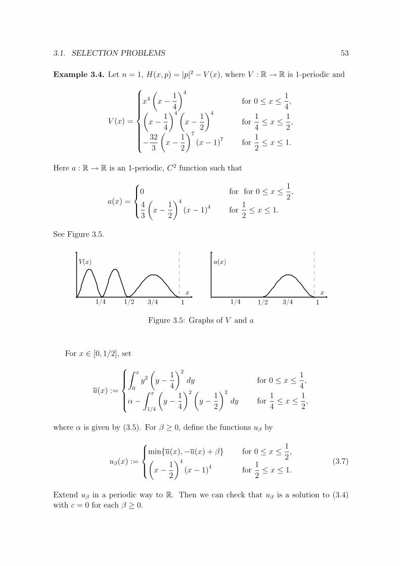
3.1. SELECTION PROBLEMS 53
Example 3.4. Let n = 1, H(x, p) = |p|2 − V (x), where V : R → R is 1-periodic and
V (x) =
x4
(x− 1
4
)4
for 0 ≤ x ≤ 1
4,(
x− 1
4
)4 (x− 1
2
)4
for1
4≤ x ≤ 1
2,
−32
3
(x− 1
2
)7
(x− 1)7 for1
2≤ x ≤ 1.
Here a : R → R is an 1-periodic, C2 function such that
a(x) =
0 for for 0 ≤ x ≤ 1
2,
4
3
(x− 1
2
)4
(x− 1)4 for1
2≤ x ≤ 1.
See Figure 3.5.
Figure 3.5: Graphs of V and a
For x ∈ [0, 1/2], set
u(x) :=
∫ x
0
y2
(y − 1
4
)2
dy for 0 ≤ x ≤ 1
4,
α−∫ x
1/4
(y − 1
4
)2 (y − 1
2
)2
dy for1
4≤ x ≤ 1
2,
where α is given by (3.5). For β ≥ 0, define the functions uβ by
uβ(x) :=
min{u(x),−u(x) + β} for 0 ≤ x ≤ 1
2,(
x− 1
2
)4
(x− 1)4 for1
2≤ x ≤ 1.
(3.7)
Extend uβ in a periodic way to R. Then we can check that uβ is a solution to (3.4)
with c = 0 for each β ≥ 0.

54 CHAPTER 3. VANISHING DISCOUNT PROBLEM
Figure 3.6: Graph of uβ on [0, 1] for β = 2α, β = α, β = 0
.
3.1.2 Discounted approximation
There are several methods to construct or approximate viscosity solutions of ergodic
problem (3.1). One natural way in terms of the well-posedness theory and a priori
estimates is the following discounted approximation procedure. For ε > 0, consider
(D)ε εuε − a(x)∆uε +H(x,Duε) = 0 in Tn.
Problem (D)ε is uniquely solvable as we see in Section 1.2 because of the term “εuε”,
which is sometimes called a discount factor in optimal control theory.
The main assumptions in this chapter are:
(H5) H ∈ C2(Tn ×Rn), p 7→ H(x, p) is convex for each x ∈ Tn, and there exists C > 0
so that
|DxH(x, p)| ≤ C(1 +H(x, p)), for all (x, p) ∈ Tn × Rn,
lim|p|→+∞
H(x, p)
|p|= +∞, uniformly for x ∈ Tn,
(H6) a ≥ 0 in Tn, and a ∈ C2(Tn).
Note that the situation we consider is a special case of general degenerate viscous case
(1.14). For the general case, see the discussion in Section 3.6.
Let us now repeat some of arguments in the proof of Theorem 1.3. Under assump-
tions (H5), (H6) (or some other appropriate growth conditions), we derive the following
a priori estimate
‖εuε‖L∞(Tn) + ‖Duε‖L∞(Tn) ≤ C for some C > 0. (3.8)
See the proof of Theorem 1.3. Once (3.8) is achieved, we obtain that
{uε(·) − uε(x0)}ε>0 is uniformly bounded and equi-Lipschitz continuous in Tn,

3.1. SELECTION PROBLEMS 55
for some fixed x0 ∈ Tn. Therefore, in view of the Arzela-Ascoli theorem, there exists a
subsequence {εj}j∈N with εj → 0 as j → ∞ such that
εjuεj → −c ∈ R, uεj − uεj(x0) → u ∈ C(Tn) uniformly in Tn as j → ∞, (3.9)
where (u, c) is a solution of ergodic problem (3.1).
Moreover, Proposition 1.6 gives{uε +
c
ε
}ε>0
is uniformly bounded and equi-Lipschitz continuous in Tn.
Thus, by using the Arzela-Ascoli theorem again, there exists a subsequence {εk}k∈Nwith εk → 0 as k → ∞ such that
uεk +c
εk
→ u ∈ C(Tn) uniformly in Tn as k → ∞, (3.10)
where (u, c) is a solution of ergodic problem (3.1).
Up to now, in convergence (3.10), we only use a soft approach mainly based on
tools from functional analysis. As explained in Introduction of this chapter, our main
question in this chapter is the selection problem concerning (D)ε, that is, whether
convergence (3.10) holds for the whole sequence ε→ 0 or not.
This problem was proposed by Lions, Papanicolaou, Varadhan [61] (see also Bardi,
Capuzzo-Dolcetta [5, Remark 1.2, page 400]). It remained unsolved for almost 30 years.
Recently, there was substantial progress in the case of convex Hamiltonians. First, a
partial characterization of the possible limits was given by Gomes [41] in terms of the
Mather measures. Iturriaga and Sanchez-Morgado [53] then studied this under rather
restricted assumptions. Davini, Fathi, Iturriaga, Zavidovique [26] and Mitake, Tran [71]
gave a positive answer for this question in case a ≡ 0 and a ≥ 0, respectively, by using
a dynamical approach and the nonlinear adjoint method. These approaches are based
on the weak KAM theory. By characterizing the limit in terms of Mather measures,
the convergence for the whole sequence is proven. A selection problem for Neumann
boundary problems conditions was examined by Al-Aidarous, Alzahrani, Ishii, Younas
[1].
We state here the main result in this chapter.
Theorem 3.1. Assume (H5), (H6) hold. For each ε > 0, let uε be the solution to (D)ε.
Then, we have that, as ε→ 0,
uε(x) +c
ε→ u0(x) := sup
φ∈Eφ(x) uniformly for x ∈ Tn, (3.11)
where we denote by E the family of solutions u of (3.1) satisfying∫∫Tn×Rn
u dµ ≤ 0 for all µ ∈ M. (3.12)
The set M, which is a family of probability measures on Tn ×Rn, is defined in Section
3.2.1.

56 CHAPTER 3. VANISHING DISCOUNT PROBLEM
Remark 3.1. (i) It is worth emphasizing that all of the above results strongly require
the convexity of the Hamiltonians. On the other hand, to obtain a priori estimate
(3.8), we only need the superlinearity of H, and in particular, we do NOT need the
convexity assumption. Thus, the question whether convergence of uε + c/ε as ε → 0
without the convexity assumption holds or not remains. Indeed, selection problems
for Hamilton–Jacobi equations with nonconvex Hamiltonians remain rather open. See
Section 3.6 for some further discussions on more recent developments.
(ii) Note also that, in the above theorem, the first-order case and the second-order case
are quite different because of the appearance of the diffusion term, which is delicate
to be handled. In particular, E is a family of solutions of (3.1) (not just subsolutions),
which is different from that of [26]. We will address this matter clearly later.
3.2 Regularizing process, stochastic Mather mea-
sures and key estimates
Hereinafter, we assume that the ergodic constant c of (3.1) is zero. Indeed, by replacing,
if necessary, H and uε by H − c and uε + c/ε, respectively, we can always reduce the
situation to the case that c = 0.
Thus, the ergodic problem is
(E) H(x,Du) = a(x)∆u in Tn.
Since uε, u are not smooth in general, in order to perform our analysis, we need a
regularizing process as in the previous chapter.
3.2.1 Regularizing process and construction of MWe denote by P(Tn ×Rn) the set of Radon probability measures on Tn ×Rn. Let the
function L : Tn × Rn → R be the Legendre transform of H. It is worth recalling the
formula of L
L(x, v) := supp∈Rn
(p · v −H(x, p)) for all (x, v) ∈ Tn × Rn.
By (H5), L is well-defined, that is, L(x, v) is finite for each (x, v) ∈ Tn × Rn. Further-
more, L is of class C1, convex with respect to v, and superlinear.
For each ε, η > 0, we study
(A)ηε εuε,η +H(x,Duε,η) = (a(x) + η2)∆uε,η in Tn,
which is an approximation of (D)ε. Due to the appearance of viscosity term η2∆uε,η,
(A)ηε has a (unique) smooth solution uε,η. The following result on the rate of conver-
gence of uε,η to uε as η → 0 is standard. It is of the same flavor as that of Proposition
2.3, and we omit its proof.

3.2. REGULARIZING PROCESS 57
Lemma 3.2. Assume (H5), (H6). Then there exists a constant C > 0 independent of
ε and η so that
‖Duε,η‖L∞(Tn) ≤ C,
‖uε,η − uε‖L∞(Tn) ≤Cη
ε.
It is time to use the nonlinear adjoint method to construct the set M ⊂ P(Tn×Rn)
in Theorem 3.1. For x0 ∈ Tn fixed, we consider an adjoint equation of the linearized
operator of (A)ηε :
(AJ)ηε εθε,η − div(DpH(x,Duε,η)θε,η) = ∆(a(x)θε,η) + η2∆θε,η + εδx0 in Tn,
where δx0 denotes the Dirac delta measure at x0. By the maximum principle and
integrating (AJ)ηε on Tn, we obtain
θε,η > 0 in Tn \ {x0}, and
∫Tn
θε,η(x) dx = 1.
In light of the Riesz theorem, for every ε, η > 0, there exists a probability measure
νε,η ∈ P(Tn × Rn) satisfying∫Tn
ψ(x,Duε,η)θε,η(x) dx =
∫∫Tn×Rn
ψ(x, p) dνε,η(x, p) (3.13)
for all ψ ∈ Cc(Tn × Rn). It is clear that supp (νε,η) ⊂ Tn × B(0, C) for some C > 0
due to Lemma 3.2. Since∫∫Tn×Rn
ψ(x, p) dνε,η(x, p) = 1 for all ε > 0, η > 0,
due to the compactness of weak convergence of measures, there exist two subsequences
ηk → 0 and εj → 0 as k → ∞, j → ∞, respectively, and probability measures
νεj , ν ∈ P(Tn × Rn) (see [30, Theorem 4] for instance) so that
νεj ,ηk ⇀ νεj as k → ∞,
νεj ⇀ ν as j → ∞,(3.14)
in the sense of measures. We also have that supp (νεj), supp (ν) ⊂ Tn × B(0, C). For
each such ν, set µ ∈ P(Tn ×Rn) so that the pushforward measure of µ associated with
Φ(x, v) = (x,DvL(x, v)) is ν, that is, for all ψ ∈ Cc(Tn × Rn),∫∫Tn×Rn
ψ(x, p) dν(x, p) =
∫∫Tn×Rn
ψ(x,DvL(x, v)) dµ(x, v). (3.15)
We denote the pushforward measure of µ by Φ#µ.
Notice that the measure µ constructed by the above process depends on the choice
of x0, {ηk}k, {εj}j, and when needed, we write µ = µ(x0, {ηk}k, {εj}j) to demonstrate

58 CHAPTER 3. VANISHING DISCOUNT PROBLEM
the clear dependence. In general, there could be many such limit µ for different choices
of x0, {ηk}k or {εj}j. We define the set M ⊂ P(Tn × Rn) by
M :=∪
x0∈Tn,{ηk}k,{εj}j
µ(x0, {ηk}k, {εj}j).
The following simple proposition records important properties of ν and µ.
Proposition 3.3. Assume that (H5), (H6) hold and the ergodic constant of (3.1) is 0.
Let ν and µ be probability measures given by (3.14) and (3.15). Then,
(i)
∫∫Tn×Rn
(DpH(x, p) · p−H(x, p)) dν(x, p) =
∫∫Tn×Rn
L(x, v) dµ(x, v) = 0,
(ii)
∫∫Tn×Rn
(DpH(x, p) ·Dϕ− a(x)∆ϕ) dν(x, p)
=
∫∫Tn×Rn
(v ·Dϕ− a(x)∆ϕ) dµ(x, v) = 0 for any ϕ ∈ C2(Tn).
Proof. Equation (A)ηε can be rewritten as
εuε,η +DpH(x,Duε,η) ·Duε,η − (a(x) + η2)∆uε,η
= DpH(x,Duε,η) ·Duε,η −H(x,Duε,η).
Multiply this by θε,η and integrate on Tn to get∫Tn
(εuε,η +DpH(x,Duε,η) ·Duε,η − (a(x) + η2)∆uε,η
)θε,η dx
=
∫Tn
(εθε,η − div (DpH(x,Duε,η)θε,η) − ∆
((a(x) + η2)θε,η
))uε,η dx
=
∫Tn
εδx0uε,η dx = εuε,η(x0).
Moreover, ∫Tn
(DpH(x,Duε,η) ·Duε,η −H(x,Duε,η)) θε,η dx
=
∫∫Tn×Rn
(DpH(x, p) · p−H(x, p)) dνε,η(x, p).
Set η = ηk, ε = εj, and let k → ∞, j → ∞ in this order to yield
0 =
∫∫Tn×Rn
(DpH(x, p) · p−H(x, p)) dν(x, p)
=
∫∫Tn×Rn
(DpH(x,DvL(x, v)) ·DvL(x, v) −H(x,DvL(x, v))) dµ(x, v)
=
∫∫Tn×Rn
L(x, v) dµ(x, v),
3.2. REGULARIZING PROCESS 59
by (3.15) and the duality of convex functions. Note in the above computation that we
have limj→∞ εjuεj(x0) = 0 because of the assumption that c = 0.
We now proceed to prove the second part. Fix ϕ ∈ C2(Tn). Multiply (AJ)ηε by ϕ
and integrate on Tn to get∫Tn
(DpH(x,Duε,η) ·Dϕ− a(x)∆ϕ) θε,η dx
= η2
∫Tn
∆ϕθε,η dx+ εϕ(x0) − ε
∫Tn
ϕθε,η dx.
We use (3.13) for ε = εj, η = ηk, and let k → ∞ to obtain∫∫Tn×Rn
(DpH(x, p) ·Dϕ− a(x)∆ϕ) dνεj(x, p)
= εjϕ(x0) − εj
∫∫Tn×Rn
ϕ(x) dνεj(x, p).
Finally, let j → ∞ to complete the proof.
Remark 3.2. It is worth emphasizing a delicate issue that we cannot replace C2 test
functions by C1,1 test functions in item (ii) of Proposition 3.3. This is because each
measure µ ∈ M can be quite singular and it can see the jumps of ∆ϕ in case ϕ is
C1,1 but not C2. This issue actually complicates our analysis later on as we need to
build C2-approximated subsolutions of (E), which is not quite standard in the theory
of viscosity solutions to second-order degenerate elliptic or parabolic equations. This
point will be addressed in Section 3.4.
Properties (i), (ii) in Proposition 3.3 of measure µ are essential ones to characterize
a stochastic Mather measure, which will be defined in the following section. This idea
was first discovered by Mane [62], who relaxed the original idea of Mather [63]. See
Fathi [34], Cagnetti, Gomes and Tran [18, Theorem 1.3] for some discussions on this.
3.2.2 Stochastic Mather measures
We are concerned with the following minimization problem
minµ∈F
∫∫Tn×Rn
L(x, v) dµ(x, v), (3.16)
where
F :=
{µ ∈ P(Tn × Rn) :
∫∫Tn×Rn
(v ·Dφ− a(x)∆φ) dµ(x, v) = 0 for all φ ∈ C2(Tn)
}.
Measures belonging to F are called holonomic measures or closing measures associated
with (3.1). By (ii) of Proposition 3.3, M ⊂ F .
Definition 3.1. We let M to be the set of all minimizers of (3.16). Each measure in
M is called a stochastic Mather measure.

60 CHAPTER 3. VANISHING DISCOUNT PROBLEM
When a ≡ 0, holonomic condition is equivalent to the invariance condition under the
Euler–Lagrange flow
d
dsDvL(γ(s), γ(s)) = DxL(γ(s), γ(s)).
This idea was first discovered by Mane [62], who relaxed the original idea of Mather
[63]. Minimizers of the minimizing problem (3.16) are precisely Mather measures for
first-order Hamilton–Jacobi equations.
When a ≡ 1, this coincides with the definition of stochastic Mather measures
for viscous Hamilton–Jacobi equations given by Gomes [39]. This means that this
definition is quite natural for the current degenerate viscous case, and it covers both
the first-order and the viscous case. Gomes [40, 41] also introduced the notion of
generalized Mather measures by using the duality principle.
Proposition 3.4. Fix µ ∈ M. Then µ is a minimizer of (3.16).
This proposition clearly implies that M ⊂ M.
Lemma 3.5. Assume that (H5), (H6) hold and the ergodic constant of (3.1) is 0. We
have ∫∫Tn×Rn
L(x, v) dµ(x, v) ≥ 0 for all µ ∈ F . (3.17)
Furthermore,
minµ∈F
∫∫Tn×Rn
L(x, v) dµ(x, v) = 0.
Since a solution w of ergodic problem (E) is not smooth in general, in order to use
the admissible condition in F , we need to find a family of smooth approximations of
w, which are approximate subsolutions to (E). A natural way to perform this task is
to use the usual convolution technique. More precisely, for each η > 0, let
wη(x) := γη ∗ w(x) =
∫Rn
γη(y)w(x+ y) dy, (3.18)
where γη(y) = η−nγ(η−1y) (here γ ∈ C∞c (Rn) is a standard symmetric mollifier such
that γ ≥ 0, supp γ ⊂ B(0, 1) and ‖γ‖L1(Rn) = 1).
In the first-order case, it is quite simple to show that {wη}η>0 indeed are approx-
imate subsolutions to (E) (see the second part of Proposition 1.5). In the current
degenerate viscous setting, it is much more complicated because of the appearance of
the possibly degenerate viscous term a(x)∆w. To prove that {wη}η>0 are approximate
subsolutions to (E), we need to be able to control the commutation term
γη ∗ (a∆w) − a(γη ∗ ∆w).
We give a commutation lemma, which itself is interesting and important:

3.2. REGULARIZING PROCESS 61
Lemma 3.6 (A commutation lemma). Assume (H5), (H6) hold. Assume that w is
a viscosity solution of (E) and wη be the function defined by (3.18) for η > 0. There
exists a constant C > 0 and a continuous function Sη : Tn → R such that
|Sη(x)| ≤ C and limη→0
Sη(x) = 0, for each x ∈ Tn, (3.19)
and
H(x,Dwη) ≤ a(x)∆wη + Sη(x) in Tn.
Moreover, we can actually show that Sη converges to 0 uniformly on Tn with con-
vergence rate η1/2, which is necessary in the proof of Theorem 3.1.
Lemma 3.7 (Uniform convergence). Assume (H5), (H6) hold. Then there exists a
universal constant C > 0 such that ‖Sη‖L∞(Tn) ≤ Cη1/2.
The proofs of Lemmas 3.6 and 3.7 are postponed to Section 3.4. By using the
commutation lemma, Lemma 3.6, we give a proof of Lemma 3.5.
Proof of Lemma 3.5 and Proposition 3.4. Let w be a solution of ergodic problem (E).
By Lemma 3.6, we have that
H(x,Dwη) ≤ a(x)∆wη + Sη(x) in Tn,
where Sη is an error term and we have a good control (3.19).
For any µ ∈ F , one has∫∫Tn×Rn
Sη(x) dµ(x, v) ≥∫∫
Tn×Rn
(H(x,Dwη) − a(x)∆wη) dµ(x, v)
≥∫∫
Tn×Rn
(−L(x, v) + (v ·Dwη − a(x)∆wη)) dµ(x, v)
= −∫∫
Tn×Rn
L(x, v) dµ(x, v),
where we use the admissible condition of µ ∈ F to go from the second line to the last
line. Thanks to (3.19), we let η → 0 and use the Lebesgue dominated convergence
theorem to deduce that ∫∫Tn×Rn
L(x, v) dµ(x, v) ≥ 0.
Thus, item (i) in Proposition 3.3 confirms that any measure µ ∈ M minimizes the
action (3.16). This is equivalent to the fact that M ⊂ M.
Remark 3.3. In general, if we do not assume that c = 0, then
minµ∈F
∫∫Tn×Rn
L(x, v) dµ(x, v) = −c.

62 CHAPTER 3. VANISHING DISCOUNT PROBLEM
3.2.3 Key estimates
In this section, we give two important estimates.
Lemma 3.8. Assume that (H5), (H6) hold and the ergodic constant of (3.1) is 0. Let
w ∈ C(Tn) be any solution of (E), and, for ε, η > 0, wη and θε,η be, respectively, the
function given by (3.18) and the solution to (AJ)ηε for some x0 ∈ Tn.
Then,
uε,η(x0) ≥ wη(x0) −∫
Tn
wηθε,η dx− Cη
ε− 1
ε
∫Tn
Sηθε,η dx, (3.20)
where Sη(x) is the function given in Lemma 3.6.
Proof. We first calculate, for every x ∈ Tn,
|∆wη(x)| ≤∫
Rn
|Dγη(y) ·Dw(x+ y)| dy
≤ C
ηn+1
∫Rn
|Dγ(η−1y)| dy =C
η
∫Rn
|Dγ(z)| dz ≤ C
η,
which immediately implies η2|∆wη| ≤ Cη. Combing this with Lemma 3.6, we see that
wη satisfies
H(x,Dwη) ≤ (a(x) + η2)∆wη + Cη + Sη(x) in Tn.
Subtract (A)ηε from the above inequality to yield
εwη + Cη + Sη(x)
≥ ε(wη − uε,η) +H(x,Dwη) −H(x,Duε,η) − (a(x) + η2)∆(wη − uε,η)
≥ ε(wη − uε,η) +DpH(x,Duε,η) ·D(wη − uε,η) − (a(x) + η2)∆(wη − uε,η),
where we use the convexity of H in the last inequality.
Then, multiplying this by θε,η, integrating on Tn, and using the integration by parts,
we get∫Tn
(εwε,η + Cη + Sη(x))θε,η dx
≥ ε
∫Tn
(wη − uε,η)θε dx+
∫Tn
(DpH(x,Duε,η) ·D(wη − uε,η) − a(x)∆(wη − uε,η)) θε,η dx
= ε
∫Tn
(wη − uε,η)θε,η dx−∫
Tn
(div (DpH(x,Duε,η)θε,η) + ∆(a(x)θε,η)) (wη − uε,η) dx
= ε
∫Tn
(wη − uε,η)θε,η dx−∫
Tn
(εθε,η − εδx0) (wη − uε,η) dx
= ε(wη − uε,η)(x0)
which, after a rearrangement, implies (3.20).

3.3. PROOF OF THEOREM 3.1 63
Proposition 3.9. Assume that (H5), (H6) hold and the ergodic constant of (3.1) is 0.
Let uε be the solution of (E)ε, and µ ∈ M. Then, for any ε > 0,∫∫Tn×Rn
uε(x) dµ(x, v) ≤ 0.
Proof. For each η > 0, we set
ψη(x) :=
∫Rn
γη(y)uε(x+ y) dy.
Thanks to Lemma 3.6, ψη satisfies
εuε +H(x,Dψη) − a(x)∆ψη ≤ Sη(x),
where |Sη(x)| ≤ C in Tn for some C > 0 independent of η, and Sη → 0 pointwise in
Tn as η → 0.
For any vector v ∈ Rn, we use the convexity of H that H(x,Dψη(x)) + L(x, v) ≥v ·Dψη(x) to obtain
εuε + v ·Dψη − L(x, v) − a(x)∆ψη ≤ Sη(x).
Thus, in light of properties (i), (ii) in Proposition 3.3 of µ, we integrate the above
inequality with respect to dµ(x, v) on Tn × Rn to imply∫∫Tn×Rn
εuε dµ(x, v) ≤∫∫
Tn×Rn
Sη(x) dµ(x, v).
Let η → 0 and use the Lebesgue dominated convergence theorem for the integral on
the right hand side of the above to complete the proof.
We remark that the key idea of Proposition 3.9 was first observed in [41, Corollary
4].
We suggest readers give the statements and the proofs of heuristic versions of
Lemma 3.8 and Proposition 3.9, in which we “assume” w, uε ∈ C∞(Tn), where w
and uε are solutions of (E), (D)ε, respectively. By doing so, one will be able to see
the clear intuitions behind the complicated technicalities. To make it rigorous, as we
see in the proofs of Lemma 3.8 and Proposition 3.9, the regularizing process and the
commutation lemma in Section 3.4 play essential roles.
3.3 Proof of Theorem 3.1
Theorem 3.1 is a straightforward consequence of the following two propositions.
Proposition 3.10. Assume that (H5), (H6) hold and the ergodic constant of (3.1) is
0. Then
lim infε→0
uε(x) ≥ u0(x).

64 CHAPTER 3. VANISHING DISCOUNT PROBLEM
Proof. Let φ ∈ E , that is, φ is a solution of (E) satisfying (3.12). Let φη = γη ∗ φ for
η > 0.
Fix x0 ∈ Tn. Take two subsequences ηk → 0 and εj → 0 so that (3.14) holds,
and limj→∞ uεj(x0) = lim infε→0 uε(x0). Let µ be the corresponding measure satisfying
ν = Φ#µ. In view of Lemmas 3.8, 3.7,
uεj ,ηk(x0) ≥ φηk(x0) −∫
Tn
φηkθεj ,ηk dx− Cηk
εj
− 1
εj
∫Tn
Sηkθεj ,ηk dx
≥ φηk(x0) −∫
Tn
φηkθεj ,ηk dx− Cηk
εj
− Cη1/2k
εj
.
Let k → ∞ to imply
uεj(x0) ≥ φ(x0) −∫∫
Tn×Rn
φ(x)dνεj(x, p).
Let j → ∞ in the above inequality to deduce further that
lim infε→0
uε(x0) = limj→∞
uεj(x0) ≥φ(x0) −∫∫
Tn×Rn
φ(x)dν(x, p)
=φ(x0) −∫∫
Tn×Rn
φ(x)dµ(x, v) ≥ φ(x0),
which implies the conclusion.
Proposition 3.11. Assume that (H5), (H6) hold and the ergodic constant of (3.1) is
0. Let {εj}j∈N be any subsequence converging to 0 such that uεj uniformly converges to
a solution u of (E) as j → ∞. Then the limit u belongs to E. In particular,
lim supε→0
uε(x) ≤ u0(x),
where u0 is the function defined in Theorem 3.1.
Proof. In view of Proposition 3.9, it is clear that any uniform limit along subse-
quences belongs to E . By the definition of the function u0, it is also obvious that
limj→∞ uεj(x) ≤ u0(x).
Remark 3.4. We discuss here four important points.
The first point is a technical one appearing in the proof of Proposition 3.10. In
order to show that
limk→∞
1
εj
∫Tn
Sηkθεj ,ηk dx = 0,
we needed to use the estimate ‖Sηk‖L∞ ≤ Cη1/2k in Lemma 3.7. The pointwise conver-
gence of Sηk to 0 in Lemma 3.6 is not enough.
Secondly, M is the collection of stochastic Mather measures that can be derived
from the solutions θε,η of the adjoint equations. It should be made clear that we do not

3.4. PROOF OF THE COMMUTATION LEMMA 65
collect all minimizing measures of (3.16) in M in general. However, we do not know
whether M ( M is true or not, where M is the set of all stochastic Mather measures
defined in Definition 3.1. This is an interesting question (though technical) worth to
be studied.
Thirdly, by repeating the whole proof, we obtain that
uε(x) → u0(x) := supφ∈eE
φ(x) uniformly for x ∈ Tn as ε→ 0, (3.21)
where we denote by E the family of solutions u of (E) satisfying∫∫Tn×Rn
u dµ ≤ 0 for all µ ∈ M.
Thus, u0 = u0. We will use this point later in Section 3.5.
Finally, as we only assume here that H is convex, and not uniformly convex in
general, we cannot expect to get deeper properties of Mather measures like Lipschitz
graph property and such. For instance, we cannot expect in our setting∫∫Tn×Rn
H(x, p) dν(x, p) = 0 for all ν given by (3.14).
It would be extremely interesting to investigate this kind of property for a degenerate
viscous Hamilton–Jacobi equation in case H is uniformly convex.
3.4 Proof of the commutation lemma
We will give a proof of the commutation lemma, Lemma 3.6, which is a technical result,
but plays a very important role in our analysis. Indeed, for each solution w of (E) with
some a priori bounds, we can construct a family of smooth approximated subsolutions
{wη}η>0 of (E). In particular, for any η > 0, wη is in C2(Tn), which is good enough for
us to use as test functions in Proposition 3.3 (ii). We have already seen this idea in
the proof of Propositions 3.4, 3.9.
It is well-known that we can perform sup-convolutions of w, which was discovered
by Jensen [55], to derive semi-convex approximated subsolutions of (E), but these are
not smooth enough to use as test functions (see Remark 3.2). It is worth pointing out
that a similar result was already discovered a long time ago by Lions [59]. However,
Lions only got that Sη converges to 0 in the almost everywhere sense, which is not
enough for our purpose. This is because each Mather measure µ can be very singular
in Tn × Rn, and the almost everywhere sense may miss some points on the support of
µ. We need to have the convergence of Sη everywhere to perform our analysis (e.g.,
the last step in the proof of Proposition 3.4).
The results related to the commutation lemma 3.6 may be of independent interests
elsewhere, and that is the reason why we present it separately here in this section. See
Section 3.6 for some further comments.

66 CHAPTER 3. VANISHING DISCOUNT PROBLEM
Proof of Lemma 3.6. It is important noting that, in view of Theorem 1.3 (see also [4,
Theorem 3.1]), all viscosity solutions of (E) are Lipschitz continuous with a universal
Lipschitz constant C. Therefore, we have
−C ≤ −a(x)∆w ≤ C in Tn
in the viscosity sense. The result of Ishii [48] on the equivalence of viscosity solutions
and solutions in the distribution sense for linear elliptic equations, and the simple
structure of a(x) allow us to conclude further that
‖Dw‖L∞(Tn) + ‖a∆w‖L∞(Tn) ≤ C (3.22)
for some constant C > 0.
Let us next show that w is actually a subsolution of (E) in the distributional sense
based on the ideas in [55]. For each δ > 0, let wδ be the sup-convolution of w, that is,
wδ(x) := supy∈Rn
(w(y) − |x− y|2
2δ
).
Thanks to [55, 23], wδ is semi-convex and is a viscosity subsolution of
−a(x)∆wδ +H(x,Dwδ) ≤ ω(δ) in Tn. (3.23)
Here, ω : (0,∞) → R is a modulus of continuity, that is, limδ→0 ω(δ) = 0. Since wδ is
a semi-convex function, it is twice differentiable almost everywhere and thus is also a
solution of (3.23) in the almost everywhere sense. We use (3.22) to deduce further that
wδ is a distributional subsolution of (3.23). By passing to a subsequence if necessary,
we obtain the following convergence
wδ → w uniformly in Tn,
Dwδ ∗⇀ Dw weakly in L∞(Tn),
as δ → 0. Take an arbitrary test function φ ∈ C2(Tn) with φ ≥ 0. We use the convexity
of H to yield that∫Tn
(H(x,Dw)φ− w∆(a(x)φ)) dx
= limδ→0
∫Tn
(H(x,Dw)φ+DpH(x,Dw) ·D(wδ − w)φ− wδ∆(a(x)φ)
)dx
≤ limδ→0
∫Tn
(H(x,Dwδ) − a∆wδ
)φ dx ≤ lim
δ→0
∫Tn
ω(δ)φ dx = 0.
Therefore, w is a subsolution of (E) in the distributional sense. For each η > 0, we
multiply (E) by γη and integrate on Tn to get
−a(x)∆wη +H(x,Dwη) ≤ Rη1(x) +Rη
2(x) in Tn,

3.4. PROOF OF THE COMMUTATION LEMMA 67
where
Rη1(x) := H(x,Dwη(x)) −
∫Rn
H(x+ y,Dw(x+ y))γη(y) dy,
Rη2(x) :=
∫Rn
a(x+ y)∆w(x+ y)γη(y) dy − a(x)∆wη(x).
We will provide treatments for Rη1 and Rη
2 separately in Lemmas 3.12 and 3.13 below.
Note that Rη2 is exactly the commutation term mentioned in Section 3.2.2.
Basically, Lemma 3.12 gives that Rη1(x) ≤ Cη for all x ∈ Tn and η > 0. Lemma
3.13 confirms that |Rη2(x)| ≤ C for all x ∈ Tn and η > 0, and limη→0R
η2(x) = 0 for
each x ∈ Tn.
We thus set Sη(x) := Cη +Rη2(x) to finish the proof.
Lemma 3.12. Assume that (H5), (H6) hold. Then there exists C > 0 independent of
η such that
Rη1(x) ≤ Cη for all x ∈ Tn and η > 0.
The proof goes essentially in the same way as that of the second part of Proposition
1.5. Nevertheless, we repeat it here to remind the readers of this simple but important
technique.
Proof. In view of (3.22) and (H5) that H ∈ C2(Tn × Rn), we have
|H(x+ y,Dw(x+ y)) −H(x,Dw(x+ y))| ≤ Cη for a.e. y ∈ B(x, η).
We then use the convexity of H and Jensen’s inequality to yield
Rη1(x) ≤H
(x,
∫Rn
γη(y)Dw(x+ y) dy
)−
∫Rn
H(x,Dw(x+ y))γη(y) dy + Cη
≤Cη.
Lemma 3.13. Assume that (H5), (H6) hold. Then there exists a constant C > 0
independent of η such that |Rη2(x)| ≤ C for all x ∈ Tn and η > 0. Moreover,
limη→0
Rη2(x) = 0 for each x ∈ Tn.
Proof. We first show the boundedness of Rη2. By using the integration by parts,
|Rη2(x)| =
∣∣∣∣∫Rn
(a(x+ y) − a(x))∆w(x+ y)γη(y) dy
∣∣∣∣=
∣∣∣∣∫Rn
γη(y)Da(x+ y) ·Dw(x+ y) dy +
∫Rn
(a(x+ y) − a(x))Dw(x+ y) ·Dγη(y) dy
∣∣∣∣≤ C
∫Rn
(γη(y) + |y| · |Dγη(y)|) dy ≤ C.

68 CHAPTER 3. VANISHING DISCOUNT PROBLEM
Next, we prove the last claim that, for each x ∈ Tn, limη→0Rη2(x) = 0. There are
two cases to be considered
(i) a(x) = 0, and (ii) a(x) > 0.
We handle case (i) first. Since a(x) = 0 = minTn a, we also have Da(x) = 0.
Therefore,
|Rη2(x)| =
∣∣∣∣∫Rn
a(x+ y)∆w(x+ y)γη(y) dy
∣∣∣∣=
∣∣∣∣∫Rn
Dw(x+ y) ·Da(x+ y)γη(y) dy +
∫Rn
Dw(x+ y) ·Dγη(y)a(x+ y) dy
∣∣∣∣≤ C
∫Rn
(|Da(x+ y)|γη(y) + a(x+ y)|Dγη(y)|) dy
= C
∫Rn
(|Da(x+ y) −Da(x)|γη(y) + (a(x+ y) − a(x) −Da(x) · y)|Dγη(y)|) dy
≤ C
∫Rn
(|y|γη(y) + |y|2|Dγη(y)|
)dy ≤ Cη.
The use of Taylor’s expansion of a(·) ∈ C2(Tn) around x is important in the above
computation.
Let us now study case (ii), in which a(x) > 0. We choose η0 > 0 sufficiently small
such that a(z) ≥ cx > 0 for |z − x| ≤ η0 for some cx > 0. In view of (3.22), we deduce
further that
|∆w(z)| ≤ C
cx=: Cx for a.e. z ∈ B(x, η0). (3.24)
Note that η0 depends on x. For η < η0, we have
|Rη2(x)| =
∣∣∣∣∫Rn
(a(x+ y) − a(x))∆w(x+ y)γη(y) dy
∣∣∣∣≤ Cx
∫Rn
|a(x+ y) − a(x)|γη(y) dy ≤ Cx
∫Rn
|y|γη(y) dy ≤ Cxη.
In both cases, we can conclude that limη→0 |Rη2(x)| = 0. Note however that the bound
for |Rη2(x)| is dependent on x.
Remark 3.5. In the proof of Lemma 3.13, estimate (3.22) plays an extremely crucial
role. That is the main reason why we require w to be a solution instead of just a
subsolution of (E) so that (3.22) holds automatically. In fact, (3.22) does not hold for
subsolutions of (E) in general. This point is one of the main difference between first-
order and second-order Hamilton–Jacobi equations. For first-order Hamilton–Jacobi
equations, that is, the case a ≡ 0, estimate (3.22) holds automatically even just for
subsolutions thanks to the coercivity of H.
We also want to comment a bit more on the rate of convergence of Rη2 in the above
proof. For each δ > 0, set U δ := {x ∈ Tn : a(x) = 0 or a(x) > δ}. Then there exists a
constant C = C(δ) > 0 such that
|Rη2(x)| ≤ C(δ)η for all x ∈ U δ.

3.4. PROOF OF THE COMMUTATION LEMMA 69
We however do not know the rate of convergence of Rη2 in Tn \ U δ through the above
proof yet.
With a more careful analysis, we are indeed able to improve the convergence rate of
Rη2 to η1/2 in Lemma 3.7 by a more careful analysis. We do not know whether this rate
is optimal or not, but for our purpose, it is good enough. See the proof of Proposition
3.10 and the first point in Remark 3.4.
Proof of Lemma 3.7. Fix x ∈ Tn and η > 0. We consider two cases
(i) miny∈B(x,η)
a(y) ≤ η, and (ii) miny∈B(x,η)
a > η.
In case (i), there exists x ∈ B(x, η) such that a(x) ≤ η. Then, in light of (2.19) (see
also [17, Lemma 2.6]), there exists a constant C > 0 such that,
|Da(x)| ≤ Ca(x)1/2 ≤ Cη1/2.
For any z ∈ B(x, η) we have the following estimates
|Da(z)| ≤ |Da(z) −Da(x)| + |Da(x)| ≤ Cη + Cη1/2 ≤ Cη1/2.
Moreover, by using Taylor’s expansion,
|a(z) − a(x)| ≤ |a(z) − a(x)| + |a(x) − a(x)|≤ |Da(x)|(|z − x| + |x− x|) + C(|z − x|2 + |x− x|2) ≤ Cη3/2 + Cη2 ≤ Cη3/2.
We use the two above inequalities to control Rη2 as
|Rη2(x)| =
∣∣∣∣∫Rn
(a(x+ y) − a(x))∆w(x+ y)γη(y) dy
∣∣∣∣=
∣∣∣∣∫Rn
Dw(x+ y) ·Da(x+ y)γη(y) dy +
∫Rn
Dw(x+ y) ·Dγη(y)(a(x+ y) − a(x)) dy
∣∣∣∣≤ C
∫Rn
(η1/2γη(y) + η3/2|Dγη(y)|
)dy ≤ Cη1/2.
Let us now consider case (ii), in which minB(x,η) a > η. A direct computation shows
|Rη2(x)| ≤
∫Rn
|(a(x+ y) − a(x))| |∆w(x+ y)| γη(y) dy
≤ C
∫Rn
|a(x+ y) − a(x)|a(x+ y)
γη(y) dy ≤ C
∫Rn
|Da(x+ y)| · |y|a(x+ y)
γη(y) dy + Cη
≤ C
∫Rn
|y|a(x+ y)1/2
γη(y) dy + Cη ≤ C
∫Rn
|y|η1/2
γη(y) dy + Cη ≤ Cη1/2.
Combining these estimates we get the conclusion.
An immediate consequence of the above lemmas is the following.

70 CHAPTER 3. VANISHING DISCOUNT PROBLEM
Lemma 3.14. Let w ∈ C(Tn) satisfy (3.22). Then, w is a viscosity subsolution of (E)
if and only if w is a subsolution of (E) in the almost everywhere sense.
Proof. Assume first that w be a viscosity subsolution of (E). Then by the first part of
the proof of Lemma 3.6, w is a subsolution of (E) in the distribution sense. In light of
(3.22), w is furthermore a subsolution of (E) in the almost everywhere sense.
On the other hand, assume that w is a subsolution of (E) in the almost everywhere
sense. For each η > 0, let wη be the function defined by (3.18). In view of Lemmas 3.7,
and the stability result of viscosity solutions, we obtain that w is a viscosity subsolution
of (E).
Another consequence of Lemmas 3.6 and 3.7 is a representation formula for ergodic
constant c in this setting. If we repeat the argument in the proof of Proposition 1.5 by
using Lemmas 3.6 and 3.7, we obtain
Proposition 3.15. Assume (H5), (H6) hold. Let c be the ergodic constant of (3.1).
Then,
c = infφ∈C2(Tn)
maxx∈Tn
(−a(x)∆φ(x) +H(x,Dφ(x))) .
See Section 3.6 for some further discussions.
3.5 Applications
Let us now discuss the limit of uε in Examples 3.1, 3.3 and 3.4 in Section 3.1.
Limit of uε in Example 3.1
In this example, the equation for uε is
εuε + |(uε)′|2 −W (x)2 = 0 in T.
By Theorem 3.1 and Remark 3.4, we have
uε(x) → u0(x)
= sup{w(x) : w is a solution to (3.2) s.t.
∫∫Tn×Rn
w dµ(x, v) ≤ 0, ∀µ ∈ M}
uniformly for x ∈ T as ε→ 0. In this specific case, we have that{δ{1/4}×{0}
}∪
{δ{3/4}×{0}
}⊂ M.
Thus,
u0(x) ≤ sup{w(x) : w is a solution to (3.2) s.t.∫∫
Tn×Rn
w dµ(x, v) ≤ 0, ∀µ ∈{δ{1/4}×{0}
}∪
{δ{3/4}×{0}
} }= sup
{w(x) : w is a solution to (3.2) s.t. w
(1/4
)≤ 0, w
(3/4
)≤ 0
},

3.5. APPLICATIONS 71
which implies u0(1/4) ≤ 0 and u0(3/4) ≤ 0. On the other hand, noting that 0 is a
subsolution of (D)ε, by the comparison principle, we have uε ≥ 0 in T, which implies
u0 ≥ 0 in R. Thus, we obtain u0(1/4) = 0 and u0(3/4) = 0, and therefore
u0 = u0 = u01 = u0
2,
where u01, u
02 are the functions defined in Example 3.1.
Figure 3.7: Graph of u0 on [0, 1]
.
Let us consider a slightly more general case:
εuε + |(uε)′ + P |2 − V (x) = 0 in T,
for P ∈ R fixed, where V ∈ C2(Tn) with V ≥ 0. Associated ergodic problem is
|u′ + P |2 − V (x) = H(P ) in T, (3.25)
where we denote the ergodic constant by H(P ) instead of c. This ergodic problem
and H(P ) are called, respectively, the cell problem and the effective Hamiltonian in
the context of periodic homogenization of Hamilton–Jacobi equations. It is well-known
that the structure of solutions to (3.25) strongly depends on P . Indeed, if
|P | ≥ P0 :=
∫T
√V (y) dy,
then solutions of (3.25) are unique (up to additive constants). On the other hand, if
|P | < P0, then solutions of (3.25) are not unique in general. See [61] for more details.
Let us therefore only consider the case where |P | < P0 here. In this case, it is
known that
δ{x0}×{0} ∈ M if and only if x0 ∈ {V = 0} := {x ∈ T : V (x) = 0}. (3.26)
See [2, 42] for instance. Therefore, by Theorem 3.1 and Remark 3.4, we obtain
uε(x) → u0(x) = sup{w(x) : w is a solution to (3.25) s.t. w ≤ 0 on {V = 0}
}uniformly for x ∈ T as ε→ 0.
We emphasize here that the characterization of Mather measures is very hard in
general. Indeed, it is still not known yet whether characterization (3.26) holds or not in
the multi-dimensional cases even in this specific form. See Section 3.6 for some further
discussions.

72 CHAPTER 3. VANISHING DISCOUNT PROBLEM
Limit of uε in Examples 3.3, 3.4
In these examples, the equation for uε is
εuε − a(x)(uε)′′ + |(uε)′|2 − V (x) = 0 in T,
where V and a are given functions in Examples 3.3, 3.4.
Firstly, let us consider Example 3.3. By Theorem 3.1 and Remark 3.4, we know
that uε uniformly converges to u0 given in (3.21). Moreover, noting that
δ{0}×{0}, δ{1/4}×{0}, δ{3/4}×{0} ∈ M,
we obtain
uε → uα uniformly for x ∈ T as ε→ 0,
where uα and α are the function and the constant given by (3.6) and (3.5), respectively.
See Figure 3.4.
Similarly, we can characterize the limit of the discount approximation for Example
3.4. Noting that
δ{0}×{0}, δ{1/4}×{0}, δ{1/2}×{0} ∈ M,
we obtain
uε → uα uniformly for x ∈ T as ε→ 0,
where uα and α are the function and the constant given by (3.7) and (3.5), respectively.
See Figure 3.6.
3.6 Some other directions and open questions
In this section, we present recent developments in the study of selection problems for
Hamilton–Jacobi equations. There are other methods to construct or approximate
viscosity solutions of the ergodic problem for Hamilton–Jacobi equations such as the
vanishing viscosity method, a finite difference approximation. If we consider a different
type of approximation for (1.6), then the selection procedure could be rather different.
Therefore, different types of difficulties may appear in general. Let us describe briefly
these directions as well as some open questions.
Discounted approximation procedure
(i) General convex settings (e.g., fully nonlinear, degenerate elliptic PDEs under
various type of boundary conditions such as periodic condition, state constraint
condition, Dirichlet condition, Neumann condition): Ishii, Mitake, Tran [51, 52]
obtained convergence results in 2016. The proofs in [51, 52] are based on a
variational approach and a duality principle, which are completely different from
the ones presented here. They nevertheless share the same philosophy.

3.6. SOME OTHER DIRECTIONS AND OPEN QUESTIONS 73
(ii) Selection problems for nonconvex Hamilton–Jacobi equations: Most problems are
open. In some examples, invariant measures and invariant sets do not exist (see
Cagnetti, Gomes, Tran [18] for the discussion on Mather measures, and Gomes,
Mitake, Tran [43] for the discussion on Aubry set). It is therefore extremely
challenging to establish general convergence results and to describe the limits if
they exist. Gomes, Mitake, Tran [43] proved convergence results for some special
nonconvex first-order cases in 2016.
(iii) Rate of convergence: It is quite challenging to obtain some rates of the con-
vergence (quantitative results) of Theorem 3.1. Mitake, Soga [67] studied this
for some special first-order situations in 2016. It is demonstrated there that er-
ror estimates would depend highly on dynamics of the corresponding dynamical
systems in general.
(iv) Aubry (uniqueness) set: The structure of solutions of (1.8) is poorly understood.
For instance, in the case of the inviscid (first-order) equation, the Aubry set
plays a key role as a uniqueness set for the ergodic problem. In a general viscous
case where the diffusion could be degenerate, there has not been any similar
notions/results on the uniqueness (Aubry) set for (1.8) up to now.
(v) Commutation lemma 3.6: Another way to perform this task is to do sup-inf-
convolution first, and usual convolution later. Ishii, Mitake, Tran did this in a
unpublished note first before finding the new variational approach in [51]. Are
these useful in other contexts?
(vi) Applications: Theorem 3.1 is very natural in its own right. It is therefore ex-
tremely interesting to use it to get some further PDE results and to find connec-
tions to dynamical systems.
Vanishing viscosity procedure
(i) Vanishing viscosity procedure: For ε > 0, consider the following problem
H(x,Duε) = ε∆uε +Hε
in Tn
where Hε
is the corresponding ergodic constant. The question of interest is to
investigate the limit of uε as ε → 0. Under relatively restrictive assumptions
on the Aubry set, the convergence is proven. See Bessi [16], Anantharaman,
Iturriaga, Padilla, Sanchez-Morgado [3]. In the general setting, there are still
many questions which are not solved yet. See also E [29] and Jauslin-Kreiss-
Moser [54] for related works on entropy solutions.
(ii) Finite difference approximation: In [75], the selection problem which appears
in the finite difference procedure was first formulated by Soga, and the conver-
gence was also proven there in a similar setting to that of the vanishing viscosity
procedure.

74 CHAPTER 3. VANISHING DISCOUNT PROBLEM
Selection of Mather measures
The fact that ergodic problems (1.6) and (1.8) have many solutions of different types
is strongly related to the multiplicity of Mather measures. Each approximation of
the ergodic problem has associated generalized Mather measures. Thus, the selection
problem for Mather measures appears. Many questions still remain open. See Anan-
tharaman [2], Evans [33], Gomes [39], Gomes, Iturriaga, Sanchez-Morgado, Yu [42], Yu
[79], Mitake, Soga [67] for this direction.

Chapter 4
Appendix
The readers can read Appendix independently from other chapters. In Appendix, we
give a short introduction to the theory of viscosity solutions of first-order Hamilton–
Jacobi equations, which was introduced by Crandall and Lions [24] (see also Crandall,
Evans, and Lions [22]). The readers can use this as a starting point to learn the theory
of viscosity solutions. Some of this short introduction is taken from the book of Evans
[31]. Let us for simplicity focus on the initial-value problem of first-order (inviscid)
Hamilton–Jacobi equations
(C)
{ut +H(x,Du) = 0 in Rn × (0,∞),
u(x, 0) = u0(x) on Rn,
where the Hamiltonian H : Rn × Rn → R and the initial function u0 : Rn → R are
given. We will give precise assumptions on H and u0 when necessary.
The original approach [24, 22, 60] is to consider the following approximated equation
(C)ε
{uε
t +H(x,Duε) = ε∆uε in Rn × (0,∞),
uε(x, 0) = u0(x) on Rn,
for ε > 0. The term ε∆uε in (C)ε regularizes the Hamilton–Jacobi equation, and this
is called the method of vanishing viscosity. We then let ε → 0 and study the limit of
the family {uε}ε>0. It is often the case that, in light of a priori estimates, {uε}ε>0 is
bounded and equicontinuous on compact subsets of Rn × [0,∞). We hence can use the
Arzela-Ascoli theorem to deduce that, there exists a subsequence {εj}j converging to
0 as j → ∞ such that,
uεj → u, locally uniformly in Rn × [0,∞),
for some limit function u ∈ C(Rn × [0,∞)). We expect that u is some kind of solution
of (C), but we only have that u is continuous and absolutely no information about Du
and ut. Also as (C) is fully nonlinear in Du and not of the divergence structure, we
cannot use integration by parts and weak convergence techniques to justify that u is
a weak solution in such sense. We instead use the maximum principle to obtain the
notion of weak solution, which is viscosity solution.
75
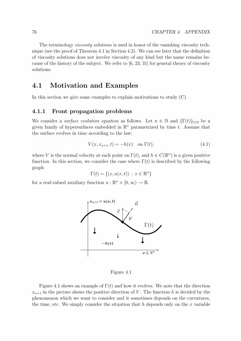
76 CHAPTER 4. APPENDIX
The terminology viscosity solutions is used in honor of the vanishing viscosity tech-
nique (see the proof of Theorem 4.1 in Section 4.2). We can see later that the definition
of viscosity solutions does not involve viscosity of any kind but the name remains be-
cause of the history of the subject. We refer to [6, 23, 31] for general theory of viscosity
solutions.
4.1 Motivation and Examples
In this section we give some examples to explain motivations to study (C).
4.1.1 Front propagation problems
We consider a surface evolution equation as follows. Let n ∈ N and {Γ(t)}t≥0 be a
given family of hypersurfaces embedded in Rn parametrized by time t. Assume that
the surface evolves in time according to the law:
V (x, xn+1, t) = −h(x) on Γ(t), (4.1)
where V is the normal velocity at each point on Γ(t), and h ∈ C(Rn) is a given positive
function. In this section, we consider the case where Γ(t) is described by the following
graph
Γ(t) = {(x, u(x, t)) : x ∈ Rn}
for a real-valued auxiliary function u : Rn × [0,∞) → R.
Figure 4.1
Figure 4.1 shows an example of Γ(t) and how it evolves. We note that the direction
xn+1 in the picture shows the positive direction of V . The function h is decided by the
phenomenon which we want to consider and it sometimes depends on the curvatures,
the time, etc. We simply consider the situation that h depends only on the x variable

4.1. MOTIVATION AND EXAMPLES 77
here. We refer to [38] for many interesting applications appearing in front propagation
problems.
Suppose that everything is smooth, and then by elementary calculations, we get
V = ~v · ~n =
(0
ut
)· 1√
1 + |Du|2
(−Du
1
)=
ut√1 + |Du|2
,
where ~v denotes the velocity in the direction xn+1. Plug this into (4.1), we get that u
is a solution to the Hamilton–Jacobi equation
ut + h(x)√
1 + |Du|2 = 0 in Rn × (0,∞).
Example 4.1. We consider the simplest case where n = 1, h(x) ≡ 1 and two initial
data: (i) a line in Figure 4.2, (ii) a curve in Figure 4.3.
Figure 4.2
Figure 4.3
In the context of large time behavior (Chapter 2), the large time limit (asymptotic
profile), if exists, is a solution to the associated ergodic problem. We also observe that
it depends on the initial data as demonstrated in Figures 4.2, 4.3. In general, it is
highly nontrivial to characterize this dependence as we deal with nonlinear equations.
Section 2.5 somehow gives an answer to this question (see Examples 2.2, 2.3 in Section
2.5).
78 CHAPTER 4. APPENDIX
4.1.2 Optimal control problems
Let L(x, v) : Rn ×Rn → R be a superlinear and convex Lagrangian with respect to the
variable v, that is, for all x, v1, v2 ∈ Rn, and λ ∈ [0, 1],L(x, v)
|v|→ ∞ locally uniformly for x ∈ Rn as |v| → ∞,
L(x, λv1 + (1 − λ)v2) ≤ λL(x, v1) + (1 − λ)L(x, v2).
Inviscid cases.
We consider the optimal control problem, for fixed (x, t) ∈ Rn × [0,∞),
Minimize
∫ t
0
L(γ(s),−γ(s)) ds+ u0(γ(t))
over all controls γ ∈ AC ([0, t],Rn) with γ(0) = x. Here u0 is a given bounded uniformly
continuous function on Rn. We denote by u(x, t) the minimum cost. It can be proven
that u solves the following Cauchy problem:{ut +H(x,Du) = 0 in Rn × (0,∞)
u(x, 0) = u0(x) on Rn,
where the Hamiltonian H is the Legendre transform of the Lagrangian L, that is,
H(x, p) = supv∈Rn
{p · v − L(x, v)} for (x, p) ∈ Rn × Rn.
Let us show a quick formal proof of this. Note first that u satisfies the so-called dynamic
programming principle, that is, for any h > 0,
u(x, t+ h) = inf
{∫ h
0
L(γ(s),−γ(s)) ds+ u(γ(h), t) : γ(0) = x
}. (4.2)
The dynamic programming principle can be checked in a rough way as following:
u(x, t+ h) =
∫ t+h
0
L(γ∗(s),−γ∗(s)) ds+ u0(γ∗(t+ h))
=
∫ h
0
L(γ∗(s),−γ∗(s)) ds+
∫ t
0
L(δ(s),−δ(s)) ds+ u0(δ(t))
=
∫ h
0
L(γ∗(s),−γ∗(s)) ds+ u(γ∗(h), t),
where we denote a minimizer of the minimizing problem for u(x, t+ h) by γ∗, and set
δ(s) := γ∗(s+ h) for s ∈ [−h, t], and we used the Bellman principle.
We rewrite it as
u(δ(−h), t+ h) − u(δ(0), t)
h=
1
h
∫ h
0
L(γ(s),−γ(s)) ds.

4.1. MOTIVATION AND EXAMPLES 79
Sending h→ 0 yields
ut +Du ·(−δ(0)
)− L
(x,−δ(0)
)= 0,
which more or less implies the conclusion. We can use this formal idea to give a rigorous
proof by performing careful computations and using the notion of viscosity solutions.
We refer to [31, 5] for details for instance.
Example 4.2 (Classical mechanics). We consider the case that L is the difference
between a kinetic energy and a potential energy, i.e., L(x, v) := |v|2/2 − V (x) for a
given function V which is uniformly bounded continuous on Rn. Then,
u(x, t) = inf
{∫ t
0
[1
2|γ(s)|2 − V (γ(s))
]ds+ u0(γ(t)) : γ ∈ AC ([0, t],Rn), γ(0) = x
}solves the following Cauchy problemut +
1
2|Du|2 + V (x) = 0 in Rn × (0,∞),
u(·, 0) = u0 on Rn.
In this case, H(x, p) = |p|2/2 + V (x).
Example 4.3 (Hopf–Lax formula). If we consider a Lagrangian which is independent
of the x variable, then we can get the Hopf–Lax formula from the optimal control
formula. In short, we have
u(x, t) = inf
{∫ t
0
L(−γ(s)) ds+ u0(γ(t)) : γ ∈ AC ([0, t],Rn), γ(0) = x
}= inf
y∈Rn
{tL
(x− y
t
)+ u0(y)
}.
It is quite straightforward to prove that the first line implies the second line in the
above by using Jensen’s inequality. We leave it to the interested readers. See [31] for
instance. We also refer to [5, 20] for the connections between the theory of viscosity
solutions and optimal control theory.
Example 4.4 (Discounted approximation). Fix δ > 0. For x ∈ Rn, define
vδ(x) = inf
{∫ ∞
0
e−δsL(γ(s),−γ(s)) ds : γ ∈ AC ([0,∞),Rn), γ(0) = x
}.
This is an infinite horizon problem in optimal control theory. The function vδ satisfies
the dynamic programming principle
vδ(x) = inf
{∫ h
0
e−δsL(γ(s),−γ(s)) ds+ e−δhvδ(γ(h)) : γ ∈ AC ([0, h],Rn), γ(0) = x
}for any h > 0. We can use this to check that vδ solves the following discount Hamilton–
Jacobi equation
δvδ +H(x,Dvδ) = 0 in Rn.
In the formula of vδ, the function e−δs plays a role of discount, and therefore, the
constant δ in the above formula is called the discount factor in optimal control theory.

80 CHAPTER 4. APPENDIX
Viscous cases.
We consider the stochastic optimal control problem
Minimize E[∫ t
0
L(Xv(s), v(s)) ds+ u0(Xv(t))
]subject to Xv = x−
∫ t
0
v(s) ds+√
2
∫ t
0
σ(Xv(s)) dWs
for x ∈ Rn, over all controls v in some admissible class, where m ∈ N and σ : Rn →Mn×m is a given matrix-valued function which is Lipschitz, and Ws denotes a standard
m-dimensional Brownian motion. Here, Mn×m denotes the set of n-by-m matrices. Let
u(x, t) be the corresponding minimum cost.
We can prove in appropriate settings that the function u solves the Cauchy problem
for the general viscous Hamilton–Jacobi equation{ut − tr
(A(x)D2u
)+H(x,Du) = 0 in Rn × (0,∞),
u(x, 0) = u0(x) on Rn,
where A(x) := σ(x)σT (x), by using the dynamic programming principle, the Ito for-
mula and the notion of viscosity solutions.
We refer to [36, 74] for the connections between the theory of viscosity solutions
and stochastic optimal control theory.
4.2 Definitions
Let us now introduce the definitions of viscosity subsolutions, supersolutions, and so-
lutions. These definitions are encoded naturally in the vanishing viscosity method (see
the proof of Theorem 4.1 below).
Definition 4.1 (Viscosity subsolutions, supersolutions, solutions). An upper semicon-
tinuous function u : Rn× [0,∞) → R is called a viscosity subsolution of the intial-value
problem (C) provided that
• u(·, 0) ≤ u0 on Rn,
• for each ϕ ∈ C1(Rn × (0,∞)), if u − ϕ has a local maximum at (x0, t0) ∈ Rn ×(0,∞) then
ϕt(x0, t0) +H(x0, Dϕ(x0, t0)) ≤ 0.
A lower semicontinuous function u : Rn× [0,∞) → R is called a viscosity supersolution
of the intial-value problem (C) provided that
• u(·, 0) ≥ u0 on Rn,

4.2. DEFINITIONS 81
• for each ϕ ∈ C1(Rn × (0,∞)), if u − ϕ has a local minimum at (x0, t0) ∈ Rn ×(0,∞) then
ϕt(x0, t0) +H(x0, Dϕ(x0, t0)) ≥ 0.
A function u : Rn × [0,∞) → R is called a viscosity solution of the intial-value problem
(C) if u is both a viscosity subsolution, and a viscosity supersolution (hence continuous)
of (C).
Remark 4.1. (i) In Definition 4.1, a local maximum (resp., minimum) can be replaced
by a maximum (resp., minimum) or even by a strict maximum (resp., minimum).
Besides, a C1 test function v can be replaced by a C∞ test function v as well.
(ii) For (x0, t0) ∈ Rn × (0,∞), we set
D+u(x0, t0) := {(ϕt(x0, t0), Dϕ(x0, t0)) :
ϕ ∈ C1 and u− ϕ has a local maximum at (x0, t0)},D−u(x0, t0) := {(ϕt(x0, t0), Dϕ(x0, t0)) :
ϕ ∈ C1 and u− ϕ has a local minimum at (x0, t0)}.
The sets D+u(x0, t0), D−u(x0, t0) are called the superdifferential and subdifferential of
u at (x0, t0), respectively. We can rewrite the definitions of viscosity subsolutions and
supersolutions by using the superdifferential and subdifferential, respectively (see [22]).
We also give the definitions of viscosity subsolutions, supersolutions, and solutions
to the following second order equation{ut + F (x,Du,D2u) = 0 in Rn × (0,∞),
u(x, 0) = u0(x) on Rn.(4.3)
Definition 4.2. An upper semicontinuous function u : Rn × [0,∞) → R is called a
viscosity subsolution of the intial-value problem (4.3) provided that
• u(·, 0) ≤ u0 on Rn,
• for any (x0, t0) ∈ Rn × (0,∞) and (a, p,X) ∈ J2,+u(x0, t0),
a+ F (x0, p,X) ≤ 0,
where
J2,+u(x0, t0) := {(ϕt(x0, t0), Dϕ(x0, t0), D2ϕ(x0, t0)) :
ϕ ∈ C2 and u− ϕ has a local maximum at (x0, t0)}.
A lower semicontinuous function u : Rn× [0,∞) → R is called a viscosity supersolution
of the intial-value problem (4.3) provided that
• u(·, 0) ≥ u0 on Rn,

82 CHAPTER 4. APPENDIX
• for any (x0, t0) ∈ Rn × (0,∞) and (a, p,X) ∈ J2,−u(x0, t0),
a+ F (x0, p,X) ≥ 0,
where
J2,−u(x0, t0) := {(ϕt(x0, t0), Dϕ(x0, t0), D2ϕ(x0, t0)) :
ϕ ∈ C2 and u− ϕ has a local minimum at (x0, t0)}.
A function u : Rn × [0,∞) → R is called a viscosity solution of the intial-value problem
(4.3) if u is both a viscosity subsolution, and a viscosity supersolution (hence continu-
ous) of (4.3).
We call J2,+u(x0, t0) and J2,−u(x0, t0) the super-semijet and sub-semijet of u at
(x0, t0), respectively.
Remark 4.2. In Definition 4.2, J2,±u(x0, t0) can be replaced by the closure of these
sets, which are defined as
J2,±u(x0, t0) := {(a, p,X) ∈ R × Rn × Mn×n
sym : ∃ (xk, tk, ak, pk, Xk) s.t.
(ak, pk, Xk) ∈ J2,±u(xk, tk) and (xk, tk, ak, pk, Xk) → (x0, t0, a, p,X) as k → ∞}.
We here give a precise result concerning the vanishing viscosity method explained
in the introduction of this appendix. It shows that Definition 4.1 arises naturally in
light of this procedure and the maximum principle. We will verify the assumption in
this theorem in Section 4.6 below.
Theorem 4.1 (Vanishing viscosity method). Let uε be the smooth solution of (C)ε for
ε > 0. Assume that there exists a subsequence {uεj}j such that
uεj → u, locally uniformly in Rn × [0,∞),
for some u ∈ C(Rn × [0,∞)) as j → ∞. Then u is a viscosity solution of (C).
Proof. We only prove that u is a viscosity subsolution of (C) as similarly we can prove
that it is a viscosity supersolution of (C). Take any ϕ ∈ C∞(Rn × (0,∞)) and assume
that u− ϕ has a strict maximum at (x0, t0) ∈ Rn × (0,∞).
Recall that uεj → u locally uniformly as j → ∞. For j large enough, uεj − ϕ has a
local maximum at some point (xj, tj) and
(xj, tj) → (x0, t0), as j → ∞.
We have
uεj
t (xj, tj) = ϕt(xj, tj), Duεj(xj, tj) = Dϕ(xj, tj), −∆uεj(xj, tj) ≥ −∆ϕ(xj, tj).

4.3. CONSISTENCY 83
Hence,
ϕt(xj, tj) +H(xj, Dϕ(xj, tj)) = uεj
t (xj, tj) +H(xj, Duεj(xj, tj))
= εj∆uεj(xj, tj) ≤ εj∆ϕ(xj, tj).
Let j → ∞ to imply that
ϕt(x0, t0) +H(x0, Dϕ(x0, t0)) ≤ 0.
Remark 4.3.
(i) Let us emphasize that obtaining viscosity solutions through the vanishing viscosity
approach is the classical approach. This method does not work for general second-order
equations. In general, we can use Perron’s method to prove the existence of viscosity
solutions.
(ii) As seen in the proof of Theorem 4.1, we lose the information of Duε and ∆uε
as ε → 0 in this argument. Evans [32] introduced the nonlinear adjoint method to
understand these in the vanishing viscosity procedure. In particular, his aim is to
understand gradient shock structures in the nonconvex setting.
4.3 Consistency
We here prove that the notion of viscosity solutions is consistent with that of classical
solutions.
Firstly, it is quite straightforward to see that if u ∈ C1(Rn × [0,∞)) solves (C)
in the classical sense, then u is a viscosity solution of (C). Next, we show that if a
viscosity solution is differentiable at some point, then it solves (C) there. We need the
following lemma.
Lemma 4.2 (Touching by a C1 function). Let m ∈ N. Assume u : Rm → R is
continuous in Rm, and is differentiable at some point x0. There exists ϕ ∈ C1(Rm)
such that u(x0) = ϕ(x0) and u− ϕ has a strict local maximum at x0.
Proof. Without loss of generality, we may assume that
x0 = 0, u(0) = 0, and Du(0) = 0. (4.4)
We use (4.4) and the differentiability of u at 0 to deduce that
u(x) = |x|ω(x), (4.5)
where ω : Rm → R is continuous with ω(0) = 0. For each r > 0, we define
ρ(r) = maxx∈B(0,r)
|ω(x)|.
We see that ρ : [0,∞) → [0,∞) is continuous, increasing, and ρ(0) = 0.

84 CHAPTER 4. APPENDIX
We define
ϕ(x) =
∫ 2|x|
|x|ρ(r)dr + |x|2, for x ∈ Rm. (4.6)
It is clear that |ϕ(x)| ≤ |x|ρ(2|x|) + |x|2, which implies
ϕ(0) = 0, Dϕ(0) = 0.
Besides, for x 6= 0, explicit computations give us that
Dϕ(x) =2x
|x|ρ(2|x|) − x
|x|ρ(|x|) + 2x,
and hence ϕ ∈ C1(Rm).
Finally, for every x 6= 0,
u(x) − ϕ(x) = |x|ω(x) −∫ 2|x|
|x|ρ(r)dr − |x|2
≤ |x|ρ(|x|) − |x|ρ(|x|) − |x|2 < 0 = u(0) − ϕ(0).
The proof is complete.
Lemma 4.2 immediately implies the following.
Theorem 4.3 (Consistency of viscosity solutions). Let u be a viscosity solution of (C),
and suppose that u is differentiable at (x0, t0) ∈ Rn × (0,∞). Then
ut(x0, t0) +H(x0, Du(x0, t0)) = 0.
4.4 Comparison principle and Uniqueness
In this section, we establish the comparison principle for (C). Let us first prepare a
useful lemma.
Lemma 4.4 (Extrema at a terminal time). Fix T > 0. Assume that u is a viscosity
subsolution (resp., supersolution) of (C). Assume further that, on Rn × (0, T ], u − ϕ
has a local maximum (resp., minimum) at a point (x0, t0) ∈ Rn × (0, T ], for some
ϕ ∈ C1(Rn × [0,∞)). Then
ϕt(x0, t0) +H(x0, Dϕ(x0, t0)) ≤ 0 (resp., ≥ 0).
The point here is that terminal time t0 = T is allowed.
Proof. We just need to verify the case of subsolution. Assume u − ϕ has a strict
maximum at (x0, T ). We define
ϕ(x, t) = ϕ(x, t) +ε
T − tfor (x, t) ∈ Rn × (0,∞)

4.4. COMPARISON PRINCIPLE AND UNIQUENESS 85
for ε > 0. If ε > 0 is small enough, then u − ϕ has a local maximum at (xε, tε) ∈Rn × (0, T ) and (xε, tε) → (x0, T ) as ε→ 0. By definition of viscosity subsolutions, we
have
ϕt(xε, tε) +H(xε, Dϕ(xε, tε)) ≤ 0
which is equivalent to
ϕt(xε, tε) +ε
(T − tε)2+H(xε, Dϕ(xε, tε)) ≤ 0.
Hence,
ϕt(xε, tε) +H(xε, Dϕ(xε, tε)) ≤ 0.
We let ε→ 0 to achieve the result.
We fix T > 0 now and consider (C) in Rn × [0, T ] only, i.e.,
(C)
{ut +H(x,Du) = 0 in Rn × (0, T ],
u(x, 0) = u0(x) on Rn.
Let us first give a formal argument to see how the comparison principle works. Let
u, v be a smooth subsolution and a smooth supersolution to (C), respectively, with
the same initial data. Our goal is to prove that u ≤ v on Rn × [0, T ]. We argue by
contradiction, and therefore we suppose that
maxRn×[0,T ]
{(u− v)(x, t) − λt} > 0
for a small λ > 0. Suppose formally that the maximum is attained at (x0, t0) ∈Rn × [0, T ). Because of the initial data, we have t0 > 0. Then,
ut(x0, t0) = vt(x0, t0) + λ, Du(x0, t0) = Dv(x0, t0).
Thus,
0 ≥ ut(x0, t0) +H(x0, Du(x0, t0)) = vt(x0, t0) + λ+H(x0, Dv(x0, t0)) ≥ λ > 0,
which is a contradiction.
We now establish the comparison principle (hence uniqueness) for (C) rigorously
by using the so-called doubling variable argument, which was originally introduced by
Kruzkov [57].
We assume further that the Hamiltonian H satisfies
(A1) There exist a positive constant C such that
|H(x, p) −H(x, q)| ≤ C|p− q|,|H(x, p) −H(y, p)| ≤ C|x− y|(1 + |p|), for (x, y, p, q) ∈ (Rn)4.

86 CHAPTER 4. APPENDIX
Theorem 4.5 (Comparison Principle for (C)). Assume that (A1) holds. If u, u are a
bounded uniformly continuous viscosity subsolution, and supersolution of (C) on Rn ×[0, T ], respectively, then u ≤ u on Rn × [0, T ].
Proof. We assume by contradiction that
supRn×[0,T ]
(u− u) = σ > 0.
For ε, λ ∈ (0, 1), we define
Φ(x, y, t, s) = u(x, t) − u(y, s) − λ(t+ s) − 1
ε2(|x− y|2 + (t− s)2) − ε(|x|2 + |y|2)
for x, y ∈ Rn, t, s ≥ 0. Since u, u are bounded, there exists a point (x0, y0, t0, s0) ∈R2n × [0, T ]2 such that
Φ(x0, y0, t0, s0) = maxR2n×[0,T ]2
Φ(x, y, t, s).
For ε, λ small enough, we have Φ(x0, y0, t0, s0) ≥ σ/2.
We use Φ(x0, y0, t0, s0) ≥ Φ(0, 0, 0, 0) to get
λ(t0 + s0) +1
ε2(|x0 − y0|2 + (t0 − s0)
2) + ε(|x0|2 + |y0|2)
≤ u(x0, t0) − u(y0, s0) − u(0, 0) + u(0, 0) ≤ C. (4.7)
Hence,
|x0 − y0| + |t0 − s0| ≤ Cε, |x0| + |y0| ≤C
ε1/2. (4.8)
We next use Φ(x0, y0, t0, s0) ≥ Φ(x0, x0, t0, t0) to deduce that
1
ε2(|x0 − y0|2 + (t0 − s0)
2) ≤ u(x0, t0) − u(y0, s0) + λ(t0 − s0) + ε(x0 − y0) · (x0 + y0).
In view of (4.8) and the uniformly continuity of u, we get
|x0 − y0|2 + (t0 − s0)2
ε2→ 0, |x0 − y0| + |t0 − s0| = o(ε) as ε→ 0. (4.9)
By (4.8) and (4.9), we can take ε > 0 small enough so that s0, t0 ≥ µ > 0 for some
µ > 0.
Notice that (x, t) 7→ Φ(x, y0, t, s0) has a maximum at (x0, t0). In view of the defini-
tion of Φ, u− ϕ has a maximum at (x0, t0) for
ϕ(x, t) := u(y0, s0) + λ(t+ s0) +1
ε2(|x− y0|2 + (t− s0)
2) + ε(|x|2 + |y0|2).
By definition of viscosity subsolutions,
λ+2(t0 − s0)
ε2+H
(x0,
2(x0 − y0)
ε2+ 2εx0
)≤ 0. (4.10)

4.4. COMPARISON PRINCIPLE AND UNIQUENESS 87
Similarly, by using the fact that (y, s) 7→ Φ(x0, y, t0, s) has a maximum at (y0, s0), we
obtain that
−λ+2(t0 − s0)
ε2+H
(y0,
2(x0 − y0)
ε2− 2εy0
)≥ 0. (4.11)
Subtracting (4.11) from (4.10), and using (4.8) and (A1) to get
2λ ≤H
(y0,
2(x0 − y0)
ε2− 2εy0
)−H
(x0,
2(x0 − y0)
ε2+ 2εx0
)≤C|x0 − y0|
(1 +
∣∣∣∣2(x0 − y0)
ε2
∣∣∣∣ + 2ε|y0|)
+ Cε|x0 − y0|.
In view of (4.9), we let ε→ 0 to discover that λ ≤ 0, which is a contradiction.
Remark 4.4. In Theorem 4.5, we assume that u, u are uniformly continuous just
to make the proof simple and clean. In fact, the comparison principle holds for the
general case that u, u are a bounded viscosity subsolution in USC (Rn × [0, T ]), and
supersolution in LSC (Rn × [0, T ]) of (C) on Rn × [0, T ], respectively. The proof for
the general case follows the same philosophy as the above one. We leave this to the
interested readers to complete.
By using the comparison principle above, we obtain the following uniqueness result
immediately.
Theorem 4.6 (Uniqueness of viscosity solution). Under assumption (A1) there exists
at most one bounded uniformly continuous viscosity solution of (C) on Rn × [0, T ].
We state here the comparison principles for stationary problems.
Theorem 4.7. Assume that (A1) holds. If v, v are a bounded uniformly continuous
viscosity subsolution, and supersolution of
v +H(x,Dv) = 0 in Rn,
respectively, then v ≤ v on Rn.
Theorem 4.8. Assume that (A1) holds. If v, v are, respectively, a bounded uniformly
continuous viscosity subsolution, and supersolution of
H(x,Dv) ≤ −δ, H(x,Dv) ≥ 0 in Rn
for δ > 0 given, then v ≤ v on Rn.
Since the proofs of Theorems 4.7, 4.8 are similar to that of Theorem 4.5, we omit
them.

88 CHAPTER 4. APPENDIX
4.5 Stability
It is really important mentioning that viscosity solutions remain stable under the L∞-
norm. The following proposition shows this basic fact.
Proposition 4.9. Let {Hk}k∈N ⊂ C(Rn × Rn) and {gk}k∈N ⊂ C(Rn). Assume that
Hk → H, gk → g locally uniformly in Rn × Rn and in Rn, respectively, as k → ∞for some H ∈ C(Rn × Rn) and g ∈ C(Rn). Let {uk}k∈N be viscosity solutions of
the Hamilton–Jacobi equations corresponding to {Hk}k∈N with uk(·, 0) = gk. Assume
furthermore that uk → u locally uniformly in Rn × [0,∞) as k → ∞ for some u ∈C(Rn × [0,∞)). Then u is a viscosity solution of (C).
Proof. It is enough to prove that u is a viscosity subsolution of (C). Take φ ∈ C1(Rn ×[0,∞)) and assume that u − φ has a strict maximum at (x0, t0) ∈ Rn × (0,∞). By
the hypothesis, for k large enough, uk − φ has a maximum at some point (xk, tk) ∈Rn × (0,∞) and (xk, tk) → (x0, t0) as k → ∞. By definition of viscosity subsolutions,
we have
φt(xk, tk) +Hk(xk, Dφ(xk, tk)) ≤ 0.
We let k → ∞ to obtain the result.
We also give useful stability results on supremum of subsolutions and infimum of
supersolutions. Let us consider
H(x,Dv) = 0 in Rn (4.12)
for simplicity.
Proposition 4.10.
(i) Let S− be a collection of subsolutions of (4.12). Define the function u on Rn by
u(x) := sup{v(x) : v ∈ S−}.
Assume that u is upper semicontinuous on Rn. Then u is a subsolution of (4.12).
(ii) Let S+ be a collection of supersolutions of (4.12). Define the function u on Rn by
u(x) := inf{v(x) : v ∈ S+}.
Assume that u is lower semicontinuous on Rn. Then u is a supersolution of (4.12).
Proof. We only prove (ii) since we can prove (i) similarly. Let φ ∈ C1(Rn), x0 ∈ Rn
and k ∈ N. Assume that u− φ has a strict minimum at x0. From the definition of u,
there exists vk ∈ S+ such that vk(x0) − 1/k < u(x0). Due to the lower semicontinuity
of u, there exists δk > 0 such that u(x0) < u(x) + 1/k for any x ∈ B(x0, δk).
Choose a sequence {xk}k∈N ⊂ B(x0, δk) so that xk → x0 and u(xk) → u(x0). We
have vk(x0) < u(xk) + 2/k for any k ∈ N. Fix r > 0. Let yk ∈ B(x0, r) be a minimum
point of vk − φ over B(x0, r) for each k ∈ N. Then, we have
yk → x0 and vk(yk) → u(x0) as k → ∞.

4.5. STABILITY 89
Indeed, we observe
u(xk) +2
k− φ(x0) > (vk − φ)(x0) ≥ (vk − φ)(yk)
≥ (u− φ)(yk) ≥ (u− φ)(x0).
From the above, we have (vk − φ)(yk) → (u − φ)(x0) and (u − φ)(yk) → (u − φ)(x0)
as k → ∞. We consider any convergent subsequence {ykj}j∈N and y0 denotes its limit
point. Noting that u is lower semicontinuous, (u − φ)(x0) = lim infk→∞(u − φ)(yk) ≥(u− φ)(y0), which guarantees yk → x0 as k → ∞. Moreover, we get vk(yk) → u(x0) as
k → ∞.
Now, by definition of viscosity supersolutions, we have
H(yk, Dφ(yk)) ≥ 0 for any k ∈ N large enough.
Sending k → ∞ yields the conclusion.
Let {uα}α∈R be a family of locally bounded functions on Rn, and define functions
u, u on Rn by
u(x) = lim supα→∞
∗uα(x) := limα→∞
sup{uβ(y) : |x− y| ≤ 1/β, β ≥ α}, (4.13)
u(x) = lim infα→∞ ∗uα(x) := lim
α→∞inf{uβ(y) : |x− y| ≤ 1/β, β ≥ α}. (4.14)
We call u and u the upper half-relaxed limit and the lower half-relaxed limit of uα
as α → ∞, respectively. Note that u and u are upper and lower semicontinuous,
respectively. We show some stability properties of u and u.
Theorem 4.11. Let {Hα}α∈R ⊂ C(Rn ×Rn). Assume that Hα → H locally uniformly
in Rn ×Rn as α→ ∞ for some H ∈ C(Rn ×Rn). Let {uα}α∈R ⊂ C(Rn) be a family of
locally uniformly bounded functions, which are solutions of (4.12). Then the half-relaxed
limits u and u are a subsolution and a supersolution of (4.12), respectively.
Lemma 4.12. Let {uα}α∈R ⊂ C(Rn) be a family of locally uniformly bounded functions,
u, u be the functions defined by (4.13) and (4.14), respectively. Assume that u − ϕ
takes a strict maximum (resp., u − ϕ takes a strict minimum) at some x0 ∈ Rn and
ϕ ∈ C1(Rn). Then there exist {xk}k∈N ⊂ Rn converging to x0 and {αk}k∈N converging
to infinity such that uαk− ϕ attains a local maximum (resp., minimum) at xk ∈ Rn,
and uαk(xk) → u(x0) (resp., uαk
(xk) → u(x0)) as k → ∞.
Proof. We only deal with the case of u. Choose {yk}k∈N ⊂ Rn so that yk → x0 and
uαk(yk) → u(x0). Let xk ∈ B(x0, r) be a maximum point of uαk
− ϕ on B(x0, r) for
r > 0. By replacing the sequence by its subsequence if necessary, we may assume
that xkj→ x ∈ B(x0, r) and uαkj
(xkj) → a ∈ R as j → ∞. Noting that uαkj
(ykj) ≤
uαkj(xkj
), sending j → ∞ yields (u − ϕ)(x0) ≤ a − ϕ(x) ≤ (u − ϕ)(x). Since x0 is
a strict maximum point of u − ϕ on Rn, we see that x = x0. Moreover, we see that
a = u(x0). Therefore, we obtain uαkj− ϕ attains a local maximum at xkj
, xkj→ x0
and uαkj(xkj
) → u(x0) as j → ∞.
90 CHAPTER 4. APPENDIX
Proof of Theorem 4.11. We only prove that u is a subsolution of (4.12). Let ϕ ∈C1(Rn) and x0 ∈ Rn. We assume that u − ϕ attains a strict maximum at x0 and let
{xk}k∈N ⊂ Rn, {αk}k∈N be the sequences obtained in Lemma 4.12. Then by definition
of viscosity solutions, we have
H(xk, Dϕ(xk)) ≤ 0 for all k ∈ N.
Sending k → ∞, we get H(x0, Dϕ(x0)) ≤ 0.
Proposition 4.13. Let {uα}α∈R ⊂ C(Rn) be uniformly bounded in Rn. Assume that
u = u =: u on K for a compact set K ⊂ Rn. Then, u ∈ C(K) and uα → u uniformly
on K as α→ ∞.
Proof. It is clear that u ∈ C(K). Suppose that uα does not uniformly converges to
u on K. Then, there exist ε0 > 0, a sequence {αk}k∈N converging to infinity, and a
sequence {xk}k∈N ⊂ K such that |uαk(xk) − u(xk)| > ε0 for any k ∈ N. Since K is
a compact set, we can extract a subsequence {xkj}j∈N such that xkj
→ x0 ∈ K as
j → ∞. Sending j → ∞ to get
ε0 ≤ lim supj→∞
(uαkj− u)(xkj
)) ≤ (u− u)(x0) = 0 or
−ε0 ≥ lim infj→∞
(uαkj− u)(xkj
)) ≥ (u− u)(x0) = 0,
which is a contradiction.
Remark 4.5. The idea of using half-relaxed limits arises naturally when attempting
to pass to the limits with maxima and minima. This result is in particular powerful
when it can be used with a comparison principle. If the comparison principle holds for
the limit equation, then a straightforward consequence of Theorem 4.11, Proposition
4.13 is that uα → u locally uniformly on Rn as α → ∞ for some u ∈ C(Rn).
If we have further that H is convex in p, then we are able to obtain more stability
results. Assume that
(A2) p 7→ H(x, p) is convex for all x ∈ Rn.
Proposition 4.14. Assume that (A2) holds. Let u be a Lipschitz continuous func-
tion on Rn. Then, u is a viscosity subsolution of (4.12) if and only if u satisfies
H(x,Du(x)) ≤ 0 for almost every x ∈ Rn.
Proof. In light of Theorem 4.3 and Rademacher’s theorem, we can easily see that if u
is a viscosity subsolution of (4.12), then u satisfies H(x,Du(x)) ≤ 0 for a.e. x ∈ Rn.
Conversely, if u satisfies H(x,Du(x)) ≤ 0 for a.e. x ∈ Rn, then by mollification, for
each ε > 0, we can construct a smooth function uε satisfying H(x,Duε) ≤ Cε in Rn as
in the proof of Proposition 1.5. Furthermore, uε → u locally uniformly in Rn as ε→ 0.
Thus, in light of the stability result, Proposition 4.9, we obtain the conclusion.
4.6. LIPSCHITZ ESTIMATES 91
Corollary 4.15. Assume that (A2) holds. Let u be a Lipschitz continuous function on
Rn. Then, u is a viscosity solution of (4.12) if and only if H(x, p) = 0 for any x ∈ Rn,
p ∈ D−u(x).
Proof. We only need to prove that u is a viscosity subsolution of (4.12) if and only if
H(x, p) ≤ 0 for any x ∈ Rn, p ∈ D−u(x). By Proposition 4.14, we have
H(x,Du(x)) ≤ 0 in Rn in the viscosity sense.
⇐⇒ H(x,Du(x)) ≤ 0 for almost every x ∈ Rn.
⇐⇒ H(x,−Dv(x)) ≤ 0 for almost every x ∈ Rn,
where v(x) = −u(x) for all x ∈ Rn.
⇐⇒ H(x,−Dv(x)) ≤ 0 in Rn in the viscosity sense.
⇐⇒ H(x,−p) ≤ 0 for any x ∈ Rn, p ∈ D+v(x).
⇐⇒ H(x, q) ≤ 0 for any x ∈ Rn, q ∈ D−u(x).
Corollary 4.16. Assume that (A2) holds.
(i) Let S− be a collection of subsolutions of (4.12). Define the function u on Rn by
u(x) := inf{v(x) : v ∈ S−}.
Assume that u is Lipschitz continuous on Rn. Then u is a subsolution of (4.12).
(ii) Let S be a collection of solutions of (4.12). Define the function u on Rn by
u(x) := inf{v(x) : v ∈ S}.
Assume that u is Lipschitz continuous on Rn. Then u is a solution of (4.12).
Taking Corollary 4.15 into account in the proof of Proposition 4.10, we are able to
prove Corollary 4.16 in a similar way. Thus, we omit the proof. Corollaries 4.15, 4.16
were first observed by Barron, Jensen [14].
4.6 Lipschitz estimates
We provide here a way to obtain Lipschitz estimates (a priori estimates) for uε, which
is the solution of (C)ε in the introduction of Appendix. Assume for simplicity the
followings
(A3) lim|p|→∞
infx∈Rn
(H(x, p)2 +DxH(x, p) · p
)= +∞.
(A4) u0 ∈ C2(Rn) and ‖u0‖C2(Rn) ≤ C < +∞.
Lemma 4.17. Assume that (A3), (A4) hold. There exists a constant C > 0 indepen-
dent of ε such that
‖uεt‖L∞(Rn×[0,∞)) + ‖Duε‖L∞(Rn×[0,∞)) ≤ C.

92 CHAPTER 4. APPENDIX
Sketch of proof. We first note that for C > 0 sufficiently large, u0±Ct are, respectively,
a supersolution and a subsolution of (C)ε. By the comparison principle, we get
u0 − Ct ≤ uε ≤ u0 + Ct.
This, together with the comparison principle once more, yields that ‖ut‖L∞(Rn×[0,∞)) ≤C.
Next, set φ := |Duε|2/2. We have
φt +DpH ·Dφ+DxH ·Duε = ε∆φ− ε|D2uε|2.
For ε > 0 sufficiently small, one has
ε|D2uε|2 ≥ 2 (ε∆uε)2 = 2(uεt +H(x,Duε))2 ≥ H(x,Duε)2 − C.
Thus,
φt +DpH ·Dφ+ (H(x,Duε)2 +DxH ·Duε − C) ≤ ε∆φ.
By the maximum principle and (A3), we get the desired result.
Theorem 4.18. Assume that (A1), (A3), (A4) hold. Then, we obtain
uε → u locally uniformly on Rn × [0,∞)
for u ∈ C(Rn × [0,∞)), where u is the unique viscosity solution of (C).
Proof. In view of Lemma 4.17, there exists a subsequence {uεj}j∈N such that
uεj → u locally uniformly on Rn × [0,∞)
for some u ∈ C(Rn × [0,∞)), which is Lipschitz. In particular, u is bounded uniformly
continuous on Rn × [0, T ] for each T > 0.
By Theorems 4.1 and 4.6, we see that u is the unique viscosity solution of (C). This
implies further that uε → u locally uniformly on Rn × [0,∞) as ε→ 0.
4.7 The Perron method
Theorem 4.19. Let f and g be a subsolution and a supersolution of (C), respectively.
Assume that f ≤ g on Rn × [0,∞). Then, the function u : Rn × [0,∞) → R defined by
u(x, t) = sup{v(x, t) : f ≤ v ≤ g on Rn × [0,∞), v is a subsolution of (C)}
is a solution of (C). Moreover, f ≤ u ≤ g on Rn × [0,∞).
The above construction of solutions is called Perron’s method. The use of this
method in the area of viscosity solutions was introduced by Ishii [47]. For simplicity
in this proof, we will assume u is continuous.

4.7. THE PERRON METHOD 93
Sketch of proof. Set
S− := {v : Rn × [0,∞) → R : f ≤ v ≤ g in Rn × [0,∞), v is a subsolution of (C)}.
Since f ∈ S−, S− 6= ∅. It is clear that f ≤ u ≤ g in Rn × [0,∞). Thus, u is locally
bounded in Rn × [0,∞) and a subsolution of (C) by Proposition 4.10.
The proof is completed by showing that u is a supersolution of (C). To do this, we
argue by contradiction, and therefore we suppose that u is not a supersolution of (C).
Then we may choose a function φ ∈ C1(Rn × (0,∞)) such that u − φ attains a strict
minimum at some (y, s) ∈ Rn × (0,∞) and φt(y, s) + H(y,Dφ(y, s)) < 0. We may
assume that (u− φ)(y, s) = 0 by adding some constant to φ.
We now prove that u(y, s) = φ(y, s) < g(y, s). Noting that u ≤ g, we deduce φ ≤ g
in Rn × (0,∞). Assume that u(y, s) = g(y, s). Then g−φ attains a minimum at (y, s).
Noting that g is a supersolution of (C), we obtain 0 ≤ φt(y, s) +H(y,Dφ(y, s)), which
contradicts the above.
Set ε0 = (g − φ)(y, s) > 0. By the continuity of g − φ and H, there exists r > 0
such that
g(x, t) ≥ φ(x, t) +ε0
2for all (x, t) ∈ B(y, r) × (s− r, s+ r),
φt(x, t) +H(x,Dφ(x, t)) ≤ 0 for all (x, t) ∈ B(y, r) × (s− r, s+ r).
Set U = B(y, r) × (s− r, s+ r) and ε = 12min{ε0,min∂U(u− φ)(x, t)} > 0. We define
the function u : Rn × [0,∞) → R by
u(x, t) :=
{max{u(x, t), φ(x, t) + ε} for (x, t) ∈ B(y, r) × (s− r, s+ r),
u(x, t) otherwise.
It is clear that u ∈ C(Rn × [0,∞)), u ≤ u and f ≤ u ≤ g in Rn × [0,∞). Besides,
u(y, s) > u(y, s) and u is a subsolution of (C), which contradicts the definition of u.


Bibliography
[1] E. S. Al-Aidarous, E. O. Alzahrani, H. Ishii, A. M. M. Younas, A convergence
result for the ergodic problem for Hamilton–Jacobi eqautions with Neumann type
boundary conditions, Proc. Roy. Soc. Edinburgh Sect. A 146 (2016) 225–242.
[2] N. Anantharaman, On the zero-temperature or vanishing viscosity limit for certain
Markov processes arising from Lagrangian dynamics, J. Eur. Math. Soc. 6 (2004),
no. 2, 207–276.
[3] N. Anantharaman, R. Iturriaga, P. Padilla, H. Sanchez-Morgado, Physical solu-
tions of the Hamilton-Jacobi equation, Discrete Contin. Dyn. Syst. Ser. B 5 (2005),
no. 3, 513–528.
[4] S. N. Armstrong, H. V. Tran, Viscosity solutions of general viscous Hamilton–
Jacobi equations, Mathematische Annalen, 361 (2015), no. 3, 647–687.
[5] M. Bardi, I. Capuzzo-Dolcetta, Optimal control and viscosity solutions of
Hamilton-Jacobi-Bellman equations, Systems & Control: Foundations & Appli-
cations. Birkhauser Boston, Inc., Boston, MA, 1997.
[6] G. Barles, Solutions de viscosite des equations de Hamilton-Jacobi, Mathematiques
& Applications (Berlin), 17, Springer-Verlag, Paris, 1994.
[7] G. Barles, H. Ishii, H. Mitake, On the large time behavior of solutions of Hamilton–
Jacobi equations associated with nonlinear boundary conditions, Arch. Ration.
Mech. Anal. 204 (2012), no. 2, 515–558.
[8] G. Barles, H. Ishii, H. Mitake, A new PDE approach to the large time asymptotics
of solutions of Hamilton-Jacobi equation, Bull. Math. Sci. 3 (2013), 363–388.
[9] G. Barles, H. Mitake, A PDE approach to large-time asymptotics for boundary-
value problems for nonconvex Hamilton-Jacobi equations, Comm. Partial Differ-
ential Equations 37 (2012), no. 1, 136–168.
[10] G. Barles, A. Porretta, T. T. Tchamba, On the large time behavior of solutions of
the Dirichlet problem for subquadratic viscous Hamilton-Jacobi equations, J. Math.
Pures Appl. (9) 94 (2010), no. 5, 497–519.
95

96 BIBLIOGRAPHY
[11] G. Barles, J.-M. Roquejoffre, Ergodic type problems and large time behaviour of un-
bounded solutions of Hamilton-Jacobi equations, Comm. Partial Differential Equa-
tions 31 (2006), no. 7-9, 1209–1225.
[12] G. Barles, P. E. Souganidis, On the large time behavior of solutions of Hamilton–
Jacobi equations, SIAM J. Math. Anal. 31 (2000), no. 4, 925–939.
[13] G. Barles, P. E. Souganidis, Space-time periodic solutions and long-time behavior
of solutions to quasi-linear parabolic equations, SIAM J. Math. Anal. 32 (2001),
no. 6, 1311–1323.
[14] E. N. Barron, R. Jensen, Semicontinuous viscosity solutions for Hamilton-Jacobi
equations with convex Hamiltonians, Comm. Partial Differential Equations 15
(1990), no. 12, 1713–1742.
[15] P. Bernard, J.-M. Roquejoffre, Convergence to time-periodic solutions in time-
periodic Hamilton-Jacobi equations on the circle, Comm. Partial Differential Equa-
tions 29 (2004), no. 3-4, 457–469.
[16] U. Bessi, Aubry-Mather theory and Hamilton-Jacobi equations, Comm. Math.
Phys. 235 (2003), no. 3, 495–511.
[17] F. Cagnetti, D. Gomes, H. Mitake, H. V. Tran, A new method for large time
behavior of convex Hamilton–Jacobi equations: degenerate equations and weakly
coupled systems, Annales de l’Institut Henri Poincare - Analyse non lineaire 32
(2015), 183–200.
[18] F. Cagnetti, D. Gomes, H. V. Tran, Aubry-Mather measures in the non convex
setting, SIAM J. Math. Anal. 43 (2011), no. 6, 2601–2629.
[19] F. Camilli, O. Ley, P. Loreti, and V. D. Nguyen, Large time behavior of weakly
coupled systems of first-order Hamilton–Jacobi equations, NoDEA Nonlinear Dif-
ferential Equations Appl., 19 (6), (2012), 719–749.
[20] P. Cannarsa and C. Sinestrari, Semiconcave functions, Hamilton-Jacobi equations,
and optimal control, Progress in Nonlinear Differential Equations and their Appli-
cations, 58. Birkhauser Boston, Inc., Boston, 2002.
[21] A. Cesaroni, M. Novaga, Long-time behavior of the mean curvature flow with pe-
riodic forcing, Comm. Partial Differential Equations 38 (2013), no. 5, 780–801.
[22] M. G. Crandall, L. C. Evans, P.-L. Lions, Some properties of viscosity solutions
of Hamilton-Jacobi equations, Trans. Amer. Math. Soc., 282 (1984), 487–502.
[23] M. G. Crandall, H. Ishii, and P.-L. Lions. User’s guide to viscosity solutions of
second order partial differential equations, Bull. Amer. Math. Soc. (N.S.), 27(1):1–
67, 1992.

BIBLIOGRAPHY 97
[24] M. G. Crandall, P.-L. Lions, Viscosity solutions of Hamilton-Jacobi equations,
Trans. Amer. Math. Soc., 277 (1983), 1–42.
[25] A. Davini, A. Siconolfi, A generalized dynamical approach to the large-time behav-
ior of solutions of Hamilton–Jacobi equations, SIAM J. Math. Anal. 38 (2006),
no. 2, 478–502.
[26] A. Davini, A. Fathi, R. Iturriaga, M. Zavidovique, Convergence of the solutions
of the discounted equation, Invent. Math. 206 (1) (2016) 29–55.
[27] A. Davini, M. Zavidovique, Aubry sets for weakly coupled systems of Hamilton-
Jacobi equations, SIAM J. Math. Anal. 46 (2014), no. 5, 3361–3389.
[28] R. J. Di Perna, P.-L. Lions, Ordinary differential equations, transport theory and
Sobolev spaces, Invent. Math. 98, 511–547 (1989).
[29] W. E, Aubry-Mather theory and periodic solutions of the forced Burgers equation,
Comm. Pure Appl. Math. 52 (1999), no. 7, 811–828.
[30] L. C. Evans, Weak convergence methods for nonlinear partial differential equations.
CBMS 74, American Mathematical Society, 1990.
[31] L. C. Evans, Partial differential equations. Second edition. Graduate Studies in
Mathematics, 19. American Mathematical Society, Providence, RI, 2010.
[32] L. C. Evans, Adjoint and compensated compactness methods for Hamilton–Jacobi
PDE, Archive for Rational Mechanics and Analysis 197 (2010), 1053–1088.
[33] L. C. Evans, Towards a quantum analog of weak KAM theory, Comm. Math. Phys.
244 (2004), no. 2, 311–334.
[34] A. Fathi, Weak KAM Theorem in Lagrangian Dynamics, to appear in Cambridge
Studies in Advanced Mathematics.
[35] A. Fathi, A. Siconolfi, Existence of C1 critical subsolutions of the Hamilton-Jacobi
equation, Invent. Math. 155 (2004), no. 2, 363–388.
[36] W. H. Fleming and H. M. Soner, Controlled Markov processes and viscosity so-
lutions, Stochastic Modelling and Applied Probability, 25. Springer, New York,
2006.
[37] Y. Fujita, H. Ishii, P. Loreti, Asymptotic solutions of viscous Hamilton-Jacobi
equations with Ornstein-Uhlenbeck operator, Comm. Partial Differential Equations
31 (2006), no. 4-6, 827–848.
[38] Y. Giga, Surface Evolution Equations. A Level Set Approach, Monographs in
Mathematics, 99. Birkhauser, Basel-Boston-Berlin (2006), xii+264pp.

98 BIBLIOGRAPHY
[39] D. A. Gomes, A stochastic analogue of Aubry-Mather theory, Nonlinearity 15
(2002), no. 3, 581–603.
[40] D. A. Gomes, Duality principles for fully nonlinear elliptic equations, Trends in
partial differential equations of mathematical physics, 125–136, Progr. Nonlinear
Differential Equations Appl., 61, Birkhauser, Basel, 2005.
[41] D. A. Gomes, Generalized Mather problem and selection principles for viscosity
solutions and Mather measures, Adv. Calc. Var., 1 (2008), 291–307.
[42] D. Gomes, R. Iturriaga, H. Sanchez-Morgado, Y. Yu, Mather measures selected by
an approximation scheme, Proc. Amer. Math. Soc. 138 (2010), no. 10, 3591–3601.
[43] D. Gomes, H. Mitake, H. V. Tran, The Selection problem for discounted Hamilton-
Jacobi equations: some non-convex cases, arXiv:1605.07532 [math.AP], submitted.
[44] N. Ichihara Large time asymptotic problems for optimal stochastic control with
superlinear cost, Stochastic Process. Appl. 122 (4) (2012), 1248–1275.
[45] N. Ichihara, H. Ishii, Long-time behavior of solutions of Hamilton-Jacobi equations
with convex and coercive Hamiltonians, Arch. Ration. Mech. Anal. 194 (2009), no.
2, 383–419.
[46] N. Ichihara, S.-J. Sheu, Large time behavior of solutions of Hamilton-Jacobi-
Bellman equations with quadratic nonlinearity in gradients, SIAM J. Math. Anal.
45 (2013), no. 1, 279–306.
[47] H. Ishii, Perron’s method for Hamilton–Jacobi equations, Duke Math Journal, 55
(1987), no. 2, 369–384.
[48] H. Ishii, On the equivalence of two notions of weak solutions, viscosity solutions
and distribution solutions, Funkcial. Ekvac. 38 (1995), no. 1, 101–120.
[49] H. Ishii, Asymptotic solutions for large-time of Hamilton–Jacobi equations in Eu-
clidean n space, Ann. Inst. H. Poincare Anal. Non Lineaire, 25 (2008), no 2,
231–266.
[50] H. Ishii, Long-time asymptotic solutions of convex Hamilton-Jacobi equations with
Neumann type boundary conditions, Calc. Var. Partial Differential Equations 42
(2011), no. 1-2, 189–209.
[51] H. Ishii, H. Mitake, H. V. Tran, The vanishing discount problem and viscosity
Mather measures. Part 1: the problem on a torus, Journal Math. Pures Appl., to
appear.
[52] H. Ishii, H. Mitake, H. V. Tran, The vanishing discount problem and viscosity
Mather measures. Part 2: boundary value problems, Journal Math. Pures Appl.,
to appear.

BIBLIOGRAPHY 99
[53] R. Iturriaga, H. Sanchez-Morgado, Limit of the infinite horizon discounted
Hamilton–Jacobi equation, Discrete Contin. Dyn. Syst. Ser. B, 15 (2011), 623–
635.
[54] H. R. Jauslin, H. O. Kreiss and J. Moser, On the forced Burgers equation with
periodic boundary conditions, Proc. Symp. Pure Math. 65 (1999), 133–153.
[55] R. Jensen, The maximum principle for viscosity solutions of fully nonlinear second
order partial differential equations, Arch. Rat. Mech. Anal. 101 (1988), 1–27.
[56] W.-L. Jin, Y. Yu, Asymptotic solution and effective Hamiltonian of a Hamilton–
Jacobi equation in the modeling of traffic flow on a homogeneous signalized road,
J. Math. Pures Appl. (9) 104 (2015), no. 5, 982–1004.
[57] S. N. Kruzkov, Generalized solutions of nonlinear equations of the first order with
several independent variables. II, (Russian) Mat. Sb. (N.S.) 72 (114) 1967 108–134.
[58] O. Ley, V. D. Nguyen, Large time behavior for some nonlinear degenerate parabolic
equations, J. Math. Pures Appl. 102 (2014), 293–314.
[59] P.-L. Lions, Control of Diffusion Processes in RN , Comm. Pure Appl. Math. 34
(1981), 121–147.
[60] P.-L. Lions, Generalized solutions of Hamilton-Jacobi equations, Research Notes
in Mathematics, Vol. 69, Pitman, Boston, Masso. London, 1982.
[61] P.-L., Lions, G. Papanicolaou, S. R. S. Varadhan, Homogenization of Hamilton–
Jacobi equations, unpublished work (1987).
[62] R. Mane, Generic properties and problems of minimizing measures of Lagrangian
systems, Nonlinearity 9 (1996), no. 2, 273–310.
[63] J. N. Mather, Action minimizing invariant measures for positive definite La-
grangian systems, Math. Z. 207 (1991), no. 2, 169–207.
[64] H. Mitake, Asymptotic solutions of Hamilton-Jacobi equations with state con-
straints, Appl. Math. Optim. 58 (2008), no. 3, 393–410.
[65] H. Mitake, The large-time behavior of solutions of the Cauchy-Dirichlet problem
for Hamilton-Jacobi equations, NoDEA Nonlinear Differential Equations App. 15
(2008), no. 3, 347–362.
[66] H. Mitake, A. Siconolfi, H. V. Tran, N. Yamada, A Lagrangian approach to weakly
coupled Hamilton-Jacobi systems, SIAM J. Math. Anal. 48 (2016), no. 2, 821–846.
[67] H. Mitake, K. Soga, Weak KAM theory for discount Hamilton-Jacobi equations
and its application, preprint.

100 BIBLIOGRAPHY
[68] H. Mitake, H. V. Tran, Remarks on the large time behavior of viscosity solutions of
quasi-monotone weakly coupled systems of Hamilton–Jacobi equations, Asymptot.
Anal. 77 (2012), 43–70.
[69] H. Mitake, H. V. Tran, A dynamical approach to the large-time behavior of so-
lutions to weakly coupled systems of Hamilton–Jacobi equations, J. Math. Pures
Appl. 101 (2014) 76–93.
[70] H. Mitake, H. V. Tran, Large-time behavior for obstacle problems for degenerate
viscous Hamilton-Jacobi equations, Calc. Var. Partial Differential Equations 54
(2015) 2039–2058.
[71] H. Mitake, H. V. Tran, Selection problems for a discount degenerate viscous
Hamilton–Jacobi equation , Adv. Math., 306 (2017), 684–703.
[72] G. Namah, J.-M. Roquejoffre, Remarks on the long time behaviour of the solutions
of Hamilton–Jacobi equations, Comm. Partial Differential Equations 24 (1999), no.
5-6, 883–893.
[73] V. D. Nguyen, Some results on the large time behavior of weakly coupled systems
of first-order Hamilton–Jacobi equations, J. Evol. Equ. 14 (2014), 299–331.
[74] M. Nisio, Stochastic Control Theory: Dynamic Programming Principle, Proba-
bility Theory and Stochastic Modelling, vol. 72. Springer, Tokyo, 2015. xvi+250
pp.
[75] K. Soga, Selection problems of Z2-periodic entropy solutions and viscosity solu-
tions, preprint (arXiv:1501.03594).
[76] D. W. Stroock and S. R. S. Varadhan, Multidimensional diffusion processes.
Reprint of the 1997 edition. Classics in Mathematics. Springer-Verlag, Berlin,
2006. xii+338 pp.
[77] T. T. Tchamba, Large time behavior of solutions of viscous Hamilton-Jacobi equa-
tions with superquadratic Hamiltonian, Asymptot. Anal. 66 (2010), no. 3-4, 161–
186.
[78] H. V. Tran, Adjoint methods for static Hamilton-Jacobi equations, Calc. Var. Par-
tial Differential Equations 41 (2011), 301–319.
[79] Y. Yu, A remark on the semi-classical measure from −h2
2∆ + V with a degenerate
potential V , Proc. Amer. Math. Soc. 135 (2007), no. 5, 1449–1454.