Jivandhar Jnawali / New Modified Newton Type Iterative Methods

24

5. Conclusion In this work, we have presented two new Newton type iterative methods having convergence order 1 +√2 and 3.5615 for solving nonlinear equations of single variable. From the numerical as well as theoretical result, the newly introduced method (3a)-(3d) whose order of convergence and efficiency index are higher than Newton’s methods and same with McDougall and Wotherspoon method (2a)-(2d). Also hybrid method (5a)-(5d) is converge to the root faster than Potra and Pta’k method but in this method we have to evaluate one more function after first iteration. References

[1]. Bradie, B. (2007). A Friendly Introduction to Numerical Analysis. Pearson Education Inc.

[2]. Dheghain, M. and Hajarian, M. (2010). New iterative method for solving nonlinear equations fourth-

order Convergence. International Journal of Computer Mathematics. 87: 834-839.

[3]. Homeier, H. H. H. (2005). On Newton’s type methods with cubic convergence. J. Comput. Appl.

Math. 176: 425–432.

[4]. Jain, D. (2013). Families of Newton-like methods with fourth-order convergence. International

Journal of Computer Mathematics. 90: 1072-1082.

[5]. Jain, P., Bhatta C.R. and Jnawali,, J. (2015) Modified Newton type methods with higher order of

convergence. Jordan J. Math. Stat. 8(4): 327–341.

[6]. Jain, P., Bhatta C.R. and Jnawali,, J. (2016). Newton type iterative methods with higher order of

convergence, J. Numer. Anal. Approx. Theory. 45: 14–26.

[7]. Jnawali, J. and Bhatta, C. R.(2018). Two higher order iterative methods for solving nonlinear

equations, Journal of the Institute of Engineering. 14: 179-18.

[8]. Jnawali, J. (2020).Some iterative methods to solve nonlinear equations with faster convergence.

Punjab University Journal of Mathematics. 52(2): 57-72.

[9]. McDougall T. J. and Wotherspoon, S. J. (2014). A simple modification of Newton’s method to

achieve convergence of order 1 + √2. Appl. Math. Letter. 29: 20-25.

[10]. ��𝑂zban, A.Y. (2004) Some new variants of Newton's method. Applied Mathematics Letters. 13: 677-682. [11]. Potra, F.A. and Pt’ak, V. (1984). Nondecrete introduction and iterative processes. Research Note

in Mathematics. Vol.203 Pitman, Bostan.

[12]. Wang, P. (2011). A third order family of Newton like iteration method for solving nonlinear

equation. Journal of Numerical Mathematics and Stochastics. 3 : 11-19. [13]. Weerakoon, S. and Fernando, T.G.I. (2002). A variant of Newton's method with accelerated third- order convergence. Applied Mathematics Letters. 13 : 87-93.

Nepal Journal of Mathematical Sciences (NJMS) Vol. 2(1), 2021 (February): 25-34 ISSN: 2738-9928 (online), 2738-9812 (print) ©© School of Mathematical Sciences, Tribhuvan University, Kathmandu, Nepal

Research Article Received Date: October 20, 2020 Accepted Date: December 27, 2020 Published Date: February 5, 2020

25

Dynamical Indicator of Human Body’s Physical Endurance

Rashmi Bhardwaj1 & Aashima Bangia University School of Basic and Applied Sciences, Non-Linear Dynamics Research Lab,

G. G. S. Indraprastha University, Dwarka, Delhi-110078. 1Corresponding Author : rashmib22@gmail.com

Abstract: Physical endurance is the time span between the beginning of physical activity by an individual and the termination because of exhaustion. Physical endurance involve a multifaceted behaviour which can be understood by complexities. Everyone performs physical activity in order to sustain-life. However, the amount of activities done are largely subject to personal choice and varies from person to person as well as for a given person over time. Physical activity like meditation/exercises are positively related to physical fitness. One needs to understand relation between physical activity, exercise, physical fitness and health. These activities can be partitioned mutually exclusively into many different ways. This paper categorizes daily physical activity into three broad subdivisions based on amount of body movements taking place are: (i) light, (ii) moderate and (iii) high intensity. These three characterizations are considered to be mutually exclusive and sum up to total energy spent by an individual. The behavior of the three factors physical activity, heart and energy generated is analyzed with the help of Fast Lyapunov indicator (FLI), Dynamic Lyapunov indicator (DLI), Small alignment index (SALI). FLI’s increase for chaotic orbits for values of R=20, Q=70 for the case of high intensity exercises and to linearly regular orbits for values of R=5, Q=8 and R=10, Q=12 in the cases of light and moderate exercises respectively. SALI’s alters through non-zero value for R=20, Q=70 while it tends to zero for values of R=5, Q=8 and R=10, Q=12. DLI’s the largest Eigen values form a definite pattern/curve for n=2000 for values of R=5, Q=8 and n=100 for R=10, Q=12 respectively as the motion stays regular plus dispersed randomly as the motion is chaotic for n=60 and for R=20, Q=70.

Keywords: Physical Endurance, Fast Lyapunov Indicators (FLIs), Dynamic Lyapunov Indicators

(DLIs), Small Alignment Indexes (SALIs), Lyapunov Characteristics Exponents (LCEs)

1. Introduction Physical activities cause body to utilise more oxygen than resting, exercising, meditating,

walking, jogging etc. which enhance and maintain physical fitness, happiness. Also, physical activities are performed for strengthening muscles, cardiovascular system, honing athletic-skills, weight loss maintenance, enjoyment. The level of physical fitness varies as amount of physical activity ranging through low to high. Dynamic exercises such as steady running, tend to produce a higher demand of the oxygen during exercise, due to the improved blood flow. On other hand, static exercises such as weight-lifting causes oxygen concentration to rise significantly. In long term, it fills an individual with happiness, refreshes & improves health.

Bhardwaj and Bangia [1] studies complex dynamics of meditating body using nonlinear analysis techniques. Bhardwaj et al [2-3, 8-9] discussed different methodologies and forecasting techniques to predict air pollution, water-pollution and weather-forecasting with the impact of pollutants on health and the dynamics of environmental and health assessment. The different tools exist to classify regular and chaotic orbits in dynamical-systems such that time series-curves, phase plots, Poincaré maps, power spectra, etc. These indicators are very powerful, but not sufficient to differentiate regular and chaotic-

1

Rashmi Bhardwaj & Aashima Bangia / Dynamical Indicator of Human Body’s Physical Endurance

26

motion when the system bears higher degrees of freedom. Buckley et al [4] discussed about the sedentary office which is a growing case for change towards better health and productivity. Buman and King [5] gave some ideas for exercise as a treatment to enhance sleep. Buskirk and Jeffris [6] discussed chaotic dynamics of coupled nonlinear oscillator. Dinas et al [7] studied the effects of exercise and physical activity on depression. The concept of FLI was proposed by Froeschle et al [10]. Grassberger and ProcacciaI [11] measured the strangeness of Strange Attractors. Lega and Froeschle [12] discussed the relationship between Fast Lyapunov Indicator and periodic-orbit for symplectic-mappings. Nonlinear Chaotic Systems discussed by Li et al [13]; Martelli [14] and Nagashima and Baba [15]. Nikić [16] discussed importance of yoga. Pimlott [17] gave some idea about miracle drugs. The concept of DLI is first coined by Saha et al [18, 19] and SALI by Skokos [20, 21].

In this paper, model consists of compartments of breathing function from physical activities towards energy produced in the body is explained. A mathematical model is developed to study the effects of physical activities on the human body and on its two major components heart and energy generated by body. The model uses non-linear differential equations which are time dependent under constant metabolic-rate. A compartment model of breath function from lungs to tissues or body cells is discussed. Also, it is considered that flow from lungs to the blood depends on the concentration present in the blood since oxygen binds to hemoglobin in the blood. In reality, this is a non-linear relationship but for simplicity, it is considered that it is directly proportional to the difference in concentrations of the twozchambers. Firstly, assumptions and factors taken into account to form the non-linear model equations are discussed. The nature and behavior of various body parts during various forms of exercise postures such as stretching, bending, standing, squatting, etc. are formulated mathematically. As, these factors change with time so, rate of change in heartbeat, lungs and blood flowing through various veins with respect to time are taken into consideration. Thus, the system of nonlinear differential equations defines the model. Phase space analysis of the system of equations is evaluated which involves calculation of equilibrium point, Jacobian matrix defining nature of the point. Further, Eigen-system leads to phase space diagram is discussed. Graphs are plotted for the equilibrium point and phase space. Time series data of the three major dynamic components i.e. Physical state of the body, Heart & Energy in the Body-cells is analyzed. This analysis is used for future predictions. Also, the graphs have been plotted for each component with time. These results are studied and various observations are made which helped in verification and a better understanding of the previously obtained results.

1. Methodology 1.1 Lyapunov Characteristic Exponents (LCE) LCEs were coined after the Russian Engineer, Alexander M. Lyapunov. Lyapunov exponent

measures relative stability of the system of equations. Multifaceted systems having Lyapunov exponents equivalent to the dimensions in the phase-space. Whenever these values are less than zero, implying nearby initial-conditions all converge to one another, and initial-small errors decrease with respect to time. However, if any of the LCE value is positive, it shows that nearby initial conditions diverge from one to another exponentially. Thus, the condition is known as sensitive dependence on initial conditions which is coined as Chaos. LCE measures the relative stability of the dynamical system(s). Number of LCEs depends on the dimension of phase-space of the system.

1.2 Dynamic Lyapunov Indicator (DLI)

DLI is categorized by the pattern formed by the largest Eigen values. When J denotes Jacobian matrix of the dynamical system. At every discretized time, calculate the eigenvalues of the matrix J and then plot the largest eigenvalue. It seems that the eigenvalues of Jacobian, J can be found as:

0J Ij

where I is the identity matrix and J is Jacobian. Whenever DLI values form a definite pattern, the motion is regular. Otherwise, DLI points get disseminated on a random basis showing no definite pattern, i.e. chaos reaching motion.

Nepal Journal of Mathematical Sciences (NJMS), Vol.2(1) , 2021 (February): 25-34

27

1.3 Fast Lyapunov Indicator (FLI)

FLI represents the value of the largest eigenvector at each iteration and also least dependent on the initial conditions. Theorem: Consider p-dimensional basis, Vp(0) = (v1(0), v2(0),...,vp(0)) entrenched into the (general notation) n-dimensional system alongwith initial condition P(0) = (x1(0), x2(0),...,xn(0)). It is taken to be the largest among the evolving vector basis outcomes at each iteration. Thus, it is calculated as:

supremum || ||, 1, 2,...,FLI v j mj

where v j is an eigenvector of eigen-basis having dimension „m‟.

Remark: Deviation norm vector approaches precipitously to totally unalike outcomes for regular vs chaotic orbits differing in huge magnitude indicating discrimination towards regular and chaotic trajectories.

For regular orbits, these are comparatively small values and for randomized orbits, FLI gets very large values. FLI increases exponentially for chaotic-orbits and linearly for regular orbits. FLI indexes present norm value for deviation vector & never computes limiting value, as .

1.4 Small Alignment Index (SALI) SALI explicitly distinguishes in ordered and chaotic-motion at each time evolution.

Theorem: Assuming „n‟ dimensional phase-diagram for the dynamical system having in general the initial condition (I.C.) as: 0 0 , 0 , , 01 2( )P x x xn . In addition to it, the deviation vector taken to be:

0 0 ,( )0 , , 01 2dx dx dxn via point, P(0) simulating alignment indexes resulting in an orbit

following evolution of trajectory with time having initial condition P(0) itself and also of two deviation vectors ,1 2t t in the beginning have two different directions.

For each time step, two-vectors deviating are: (t)1 ; ( )2 t need to be stabilized. Then, SALI is:

( ) ( ) ( ) ( )1 2 1 2( ) minimum ,|| ( ) || || ( ) || || ( ) || || ( ) ||1 2 1 2

t t t tSALI t

t t t t

For the case of n-dimensional system where 2n , SALI oscillates through non-zero-value for ordered-orbits. SALI value tending towards zero in the chaotic trajectories. For 2D mapping, the alignment index tends to zero both for ordered-and-chaotic orbits following however, completely different time-rates, to distinguish between the two cases.

Attractors: The two types of the attractors that are to be studied are: 1. Equilibrium: 0 > 1 2 3 … n ;

2. Strange chaotic: 0, 01 1

nii

.

Mathematical Modeling The mathematical model for three important components: Physical state of the body, Heart and

Energy generated in cells/tissues of the body is proposed. The model helps to study the impact of exercises on these factors simultaneously with time and also to study how the change in one component influences the changes in other with respect to time. For the development of model some assumptions that are required to transform the biological condition into a mathematical model are as follows: The core assumption considered for modeling the problem states that oxygen comes in and goes out

of the lungs during various physical activities like walking, exercising, resting etc. where breathing

Rashmi Bhardwaj & Aashima Bangia / Dynamical Indicator of Human Body’s Physical Endurance

26

motion when the system bears higher degrees of freedom. Buckley et al [4] discussed about the sedentary office which is a growing case for change towards better health and productivity. Buman and King [5] gave some ideas for exercise as a treatment to enhance sleep. Buskirk and Jeffris [6] discussed chaotic dynamics of coupled nonlinear oscillator. Dinas et al [7] studied the effects of exercise and physical activity on depression. The concept of FLI was proposed by Froeschle et al [10]. Grassberger and ProcacciaI [11] measured the strangeness of Strange Attractors. Lega and Froeschle [12] discussed the relationship between Fast Lyapunov Indicator and periodic-orbit for symplectic-mappings. Nonlinear Chaotic Systems discussed by Li et al [13]; Martelli [14] and Nagashima and Baba [15]. Nikić [16] discussed importance of yoga. Pimlott [17] gave some idea about miracle drugs. The concept of DLI is first coined by Saha et al [18, 19] and SALI by Skokos [20, 21].

In this paper, model consists of compartments of breathing function from physical activities towards energy produced in the body is explained. A mathematical model is developed to study the effects of physical activities on the human body and on its two major components heart and energy generated by body. The model uses non-linear differential equations which are time dependent under constant metabolic-rate. A compartment model of breath function from lungs to tissues or body cells is discussed. Also, it is considered that flow from lungs to the blood depends on the concentration present in the blood since oxygen binds to hemoglobin in the blood. In reality, this is a non-linear relationship but for simplicity, it is considered that it is directly proportional to the difference in concentrations of the twozchambers. Firstly, assumptions and factors taken into account to form the non-linear model equations are discussed. The nature and behavior of various body parts during various forms of exercise postures such as stretching, bending, standing, squatting, etc. are formulated mathematically. As, these factors change with time so, rate of change in heartbeat, lungs and blood flowing through various veins with respect to time are taken into consideration. Thus, the system of nonlinear differential equations defines the model. Phase space analysis of the system of equations is evaluated which involves calculation of equilibrium point, Jacobian matrix defining nature of the point. Further, Eigen-system leads to phase space diagram is discussed. Graphs are plotted for the equilibrium point and phase space. Time series data of the three major dynamic components i.e. Physical state of the body, Heart & Energy in the Body-cells is analyzed. This analysis is used for future predictions. Also, the graphs have been plotted for each component with time. These results are studied and various observations are made which helped in verification and a better understanding of the previously obtained results.

1. Methodology 1.1 Lyapunov Characteristic Exponents (LCE) LCEs were coined after the Russian Engineer, Alexander M. Lyapunov. Lyapunov exponent

measures relative stability of the system of equations. Multifaceted systems having Lyapunov exponents equivalent to the dimensions in the phase-space. Whenever these values are less than zero, implying nearby initial-conditions all converge to one another, and initial-small errors decrease with respect to time. However, if any of the LCE value is positive, it shows that nearby initial conditions diverge from one to another exponentially. Thus, the condition is known as sensitive dependence on initial conditions which is coined as Chaos. LCE measures the relative stability of the dynamical system(s). Number of LCEs depends on the dimension of phase-space of the system.

1.2 Dynamic Lyapunov Indicator (DLI)

DLI is categorized by the pattern formed by the largest Eigen values. When J denotes Jacobian matrix of the dynamical system. At every discretized time, calculate the eigenvalues of the matrix J and then plot the largest eigenvalue. It seems that the eigenvalues of Jacobian, J can be found as:

0J Ij

where I is the identity matrix and J is Jacobian. Whenever DLI values form a definite pattern, the motion is regular. Otherwise, DLI points get disseminated on a random basis showing no definite pattern, i.e. chaos reaching motion.

Nepal Journal of Mathematical Sciences (NJMS), Vol.2(1) , 2021 (February): 25-34

27

1.3 Fast Lyapunov Indicator (FLI)

FLI represents the value of the largest eigenvector at each iteration and also least dependent on the initial conditions. Theorem: Consider p-dimensional basis, Vp(0) = (v1(0), v2(0),...,vp(0)) entrenched into the (general notation) n-dimensional system alongwith initial condition P(0) = (x1(0), x2(0),...,xn(0)). It is taken to be the largest among the evolving vector basis outcomes at each iteration. Thus, it is calculated as:

supremum || ||, 1, 2,...,FLI v j mj

where v j is an eigenvector of eigen-basis having dimension „m‟.

Remark: Deviation norm vector approaches precipitously to totally unalike outcomes for regular vs chaotic orbits differing in huge magnitude indicating discrimination towards regular and chaotic trajectories.

For regular orbits, these are comparatively small values and for randomized orbits, FLI gets very large values. FLI increases exponentially for chaotic-orbits and linearly for regular orbits. FLI indexes present norm value for deviation vector & never computes limiting value, as .

1.4 Small Alignment Index (SALI) SALI explicitly distinguishes in ordered and chaotic-motion at each time evolution.

Theorem: Assuming „n‟ dimensional phase-diagram for the dynamical system having in general the initial condition (I.C.) as: 0 0 , 0 , , 01 2( )P x x xn . In addition to it, the deviation vector taken to be:

0 0 ,( )0 , , 01 2dx dx dxn via point, P(0) simulating alignment indexes resulting in an orbit

following evolution of trajectory with time having initial condition P(0) itself and also of two deviation vectors ,1 2t t in the beginning have two different directions.

For each time step, two-vectors deviating are: (t)1 ; ( )2 t need to be stabilized. Then, SALI is:

( ) ( ) ( ) ( )1 2 1 2( ) minimum ,|| ( ) || || ( ) || || ( ) || || ( ) ||1 2 1 2

t t t tSALI t

t t t t

For the case of n-dimensional system where 2n , SALI oscillates through non-zero-value for ordered-orbits. SALI value tending towards zero in the chaotic trajectories. For 2D mapping, the alignment index tends to zero both for ordered-and-chaotic orbits following however, completely different time-rates, to distinguish between the two cases.

Attractors: The two types of the attractors that are to be studied are: 1. Equilibrium: 0 > 1 2 3 … n ;

2. Strange chaotic: 0, 01 1

nii

.

Mathematical Modeling The mathematical model for three important components: Physical state of the body, Heart and

Energy generated in cells/tissues of the body is proposed. The model helps to study the impact of exercises on these factors simultaneously with time and also to study how the change in one component influences the changes in other with respect to time. For the development of model some assumptions that are required to transform the biological condition into a mathematical model are as follows: The core assumption considered for modeling the problem states that oxygen comes in and goes out

of the lungs during various physical activities like walking, exercising, resting etc. where breathing

Rashmi Bhardwaj & Aashima Bangia / Dynamical Indicator of Human Body’s Physical Endurance

28

function is denoted by R in volume per time units i.e., the concentration of oxygen in the body cells changes with time.

Depending on the oxygen capacity of lungs, relevant amount of oxygen goes into the heart. Even after this process, there is a possibility that some amount i.e. minimal volume equivalent to 1.2L of oxygen remains in the lungs.

The variation in oxygen levels in the lung during exercising (specifically, exhaling) is also taken into account. It is assumed that the amount of movement from lungs to the heart can be governed by the concentration streamlined into bloodstream; as oxygen fixes to haemoglobin of blood.

Oxygen drifts from blood towards body cells where energy for performing activities is produced. Lastly, oxygen consumption is proportional to amount obtainable having metabolic rate (M).

The Compartmental model is given as follows:

Assuming non-linearity in the system having x that denotes concentration of oxygen flow during any physical state (like exercising, walking, resting) of human body, y representing the concentration of oxygen flow in heart/bloodstream during a particular physical state of body and variable z to represent the concentration of oxygen in body/cells. These three variables fluctuating rates with respect to time are thought of as three new state-variables. Let M represents metabolic-rate i.e., how much oxygen is utilized in body; R denotes the breath function and for Inhaling rate: R > 0; Exhaling rate: R < 0; η refers to the maximum transfer rate of molecules from the lungs towards bloodstream; f denotes the max transfer rate of molecules through bloodstream to body tissues; the max lung-volume is denoted by V. Let p refers to period of breath, t accounting for breathing-period, Q denotes amount of oxygen intake for various conditions of heart (24 L/min). All the concentration are taken to be positive-i.e., x 0, zy 0, zz 0. Therefore, assigning an appropriate dimension to every state-variable, following simplified-model is obtained:

'[t] ( ) RC (1)y'[t] ( ) (2)z'[t] M (3)

x ax b x yx b z dyx y z dy

where, x[t]-concentration of oxygen flow during any physical state (like exercising, walking, resting) of human body, y[t]-concentration of oxygen flow in heart/bloodstream during a particular physical state of body and z[t]-concentration of oxygen in body/cells. Also, a = sqrt(R)/Vol, b = η, C=Q, d = f. As per simulations carried out, following included parameters have constant values in equations (1) - (3) to be considered as follows:

Vol=3600 ml, η = z 0.1/s, f =0.7/s, M= 0.01/s, Qmax = 24L/min, R = 20s. R is deliberated from the tidal volume (about 500ml) for the customary breathing function and the maximum lung volume was used and the breath-rate is defined as 20s inhale, 20s suspension, and 20s exhale.

3. Results and Discussion Critical (or more commonly called fixed) points of the system where the changes in the system’s behavior/orbits are obtained through equations of system (1), (2) & (3), i.e. x'(t) = 0, y'(t) = 0 and z'(t) = 0 which are

- b( - ) = 0

( - z) - = 0

- M + = 0

RC+ax x y

x b dy

xy z dy

Jacobian for system of equation (1) – (3) can be given by

Heart/Bloodstream (y(t))

Energy in Body cells (z(t)) Physical state of

the body (x(t))

Nepal Journal of Mathematical Sciences (NJMS), Vol.2(1) , 2021 (February): 25-34

29

1 * * * 0

* * 1 * *

* * * 1 *

a k b k b k

J b k k z t d k k x t

k y t d k k x t k M

The Characteristic equation from the Jacobian Matrix is given as: 3 + b12 + b2 + b3 = 0 where,

1

2 2 2 2 22

2 2 2 2 2 2

2 2 2 2 2 2 23

2 3 3 3 2 3 3 2 2

(3 ak bk dk kM);

( 3 2ak 2 bk 2dk b k adk bdk 2 kM ak M)

bk M dk M dk x[t] k x[t] bk z[t];

(1 ak bk dk b k adk bdk kM ak M bk M dk M

b k M [ ] [ ] [ ] [ ]

b

b

b

adk M bdk M dk x t adk x t bdk x t k x t

3 2 3 2 3 2 3[t] bk x[t] bk x[t] y[t] bk z[t] bk Mz[t])ak x

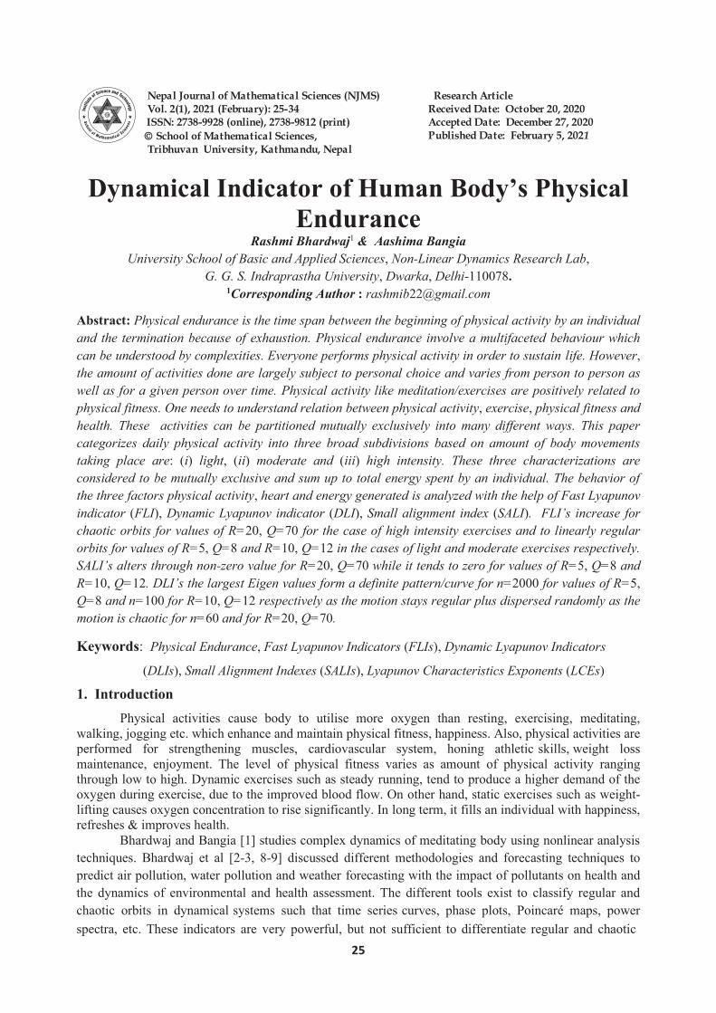
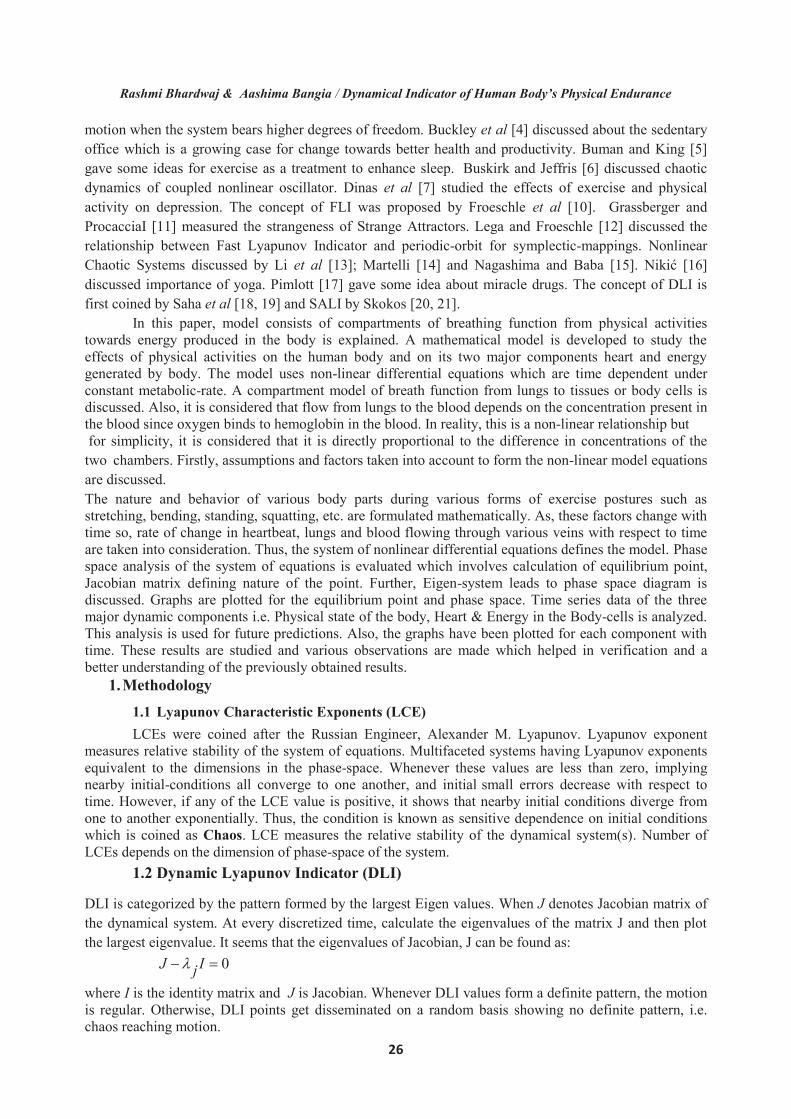
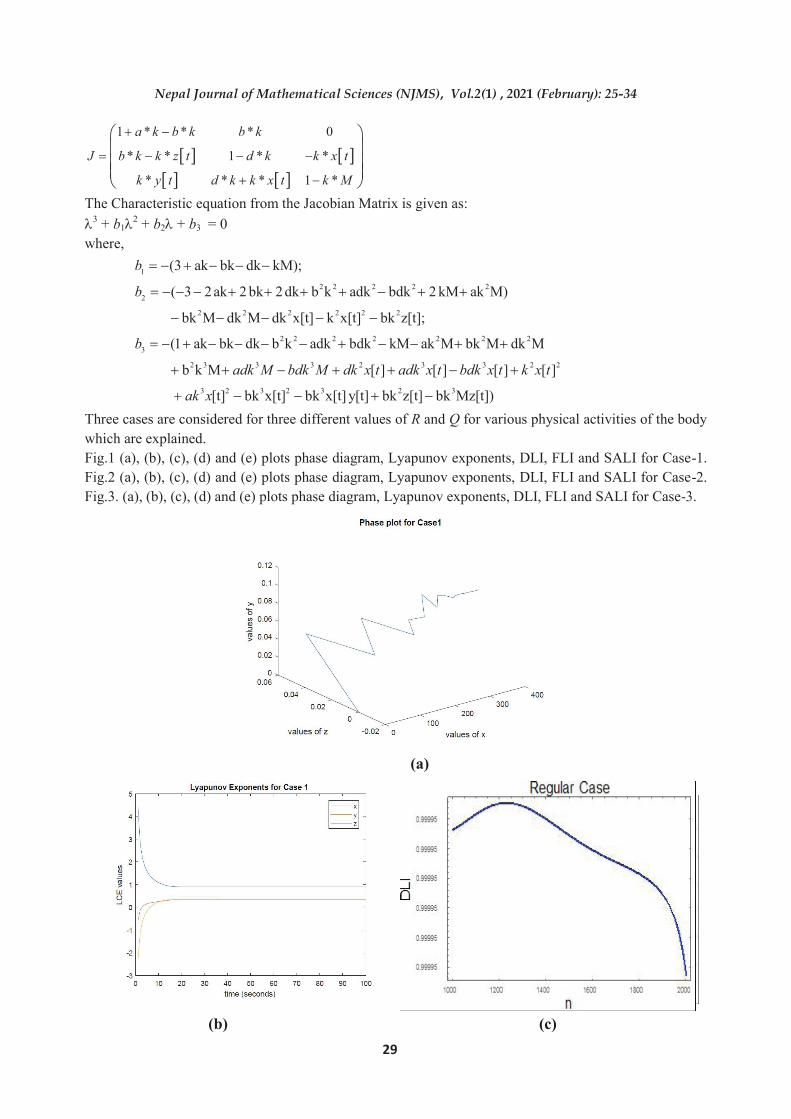
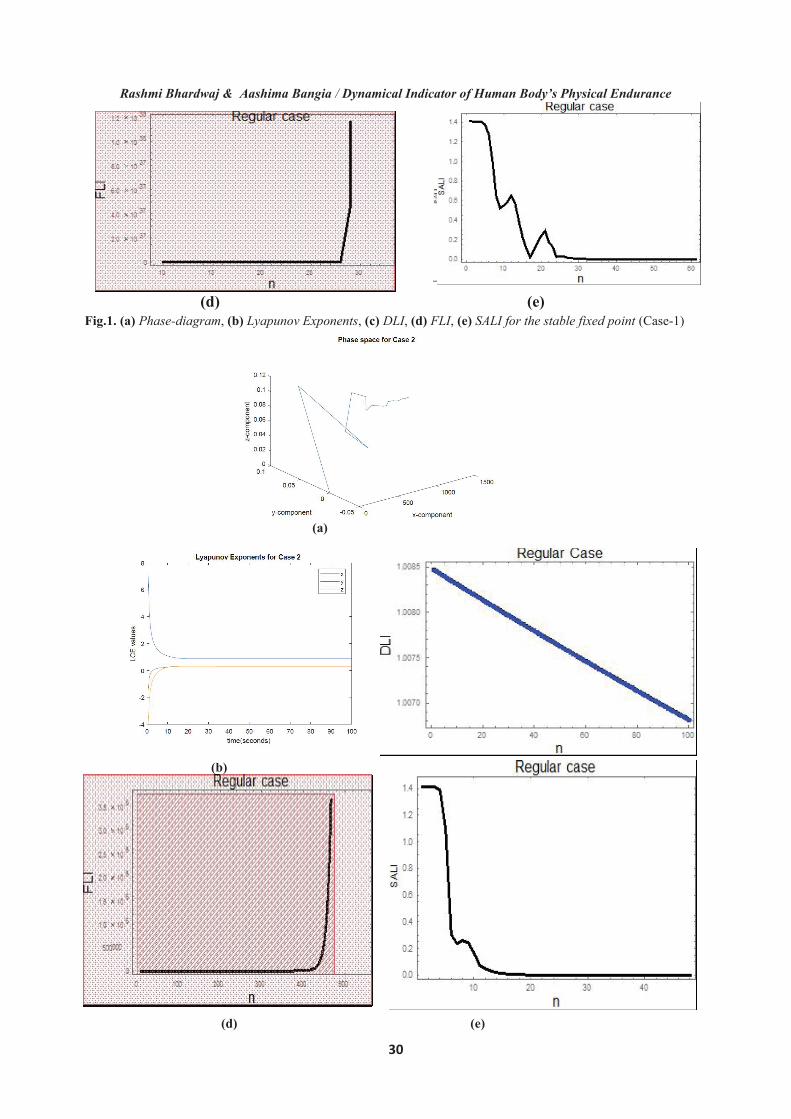
Three cases are considered for three different values of R and Q for various physical activities of the body which are explained. Fig.1 (a), (b), (c), (d) and (e) plots phase diagram, Lyapunov exponents, DLI, FLI and SALI for Case-1. Fig.2 (a), (b), (c), (d) and (e) plots phase diagram, Lyapunov exponents, DLI, FLI and SALI for Case-2. Fig.3. (a), (b), (c), (d) and (e) plots phase diagram, Lyapunov exponents, DLI, FLI and SALI for Case-3.

(a)

(b) (c)

Rashmi Bhardwaj & Aashima Bangia / Dynamical Indicator of Human Body’s Physical Endurance

28

function is denoted by R in volume per time units i.e., the concentration of oxygen in the body cells changes with time.

Depending on the oxygen capacity of lungs, relevant amount of oxygen goes into the heart. Even after this process, there is a possibility that some amount i.e. minimal volume equivalent to 1.2L of oxygen remains in the lungs.

The variation in oxygen levels in the lung during exercising (specifically, exhaling) is also taken into account. It is assumed that the amount of movement from lungs to the heart can be governed by the concentration streamlined into bloodstream; as oxygen fixes to haemoglobin of blood.

Oxygen drifts from blood towards body cells where energy for performing activities is produced. Lastly, oxygen consumption is proportional to amount obtainable having metabolic rate (M).

The Compartmental model is given as follows:

Assuming non-linearity in the system having x that denotes concentration of oxygen flow during any physical state (like exercising, walking, resting) of human body, y representing the concentration of oxygen flow in heart/bloodstream during a particular physical state of body and variable z to represent the concentration of oxygen in body/cells. These three variables fluctuating rates with respect to time are thought of as three new state-variables. Let M represents metabolic-rate i.e., how much oxygen is utilized in body; R denotes the breath function and for Inhaling rate: R > 0; Exhaling rate: R < 0; η refers to the maximum transfer rate of molecules from the lungs towards bloodstream; f denotes the max transfer rate of molecules through bloodstream to body tissues; the max lung-volume is denoted by V. Let p refers to period of breath, t accounting for breathing-period, Q denotes amount of oxygen intake for various conditions of heart (24 L/min). All the concentration are taken to be positive-i.e., x 0, zy 0, zz 0. Therefore, assigning an appropriate dimension to every state-variable, following simplified-model is obtained:

'[t] ( ) RC (1)y'[t] ( ) (2)z'[t] M (3)

x ax b x yx b z dyx y z dy

where, x[t]-concentration of oxygen flow during any physical state (like exercising, walking, resting) of human body, y[t]-concentration of oxygen flow in heart/bloodstream during a particular physical state of body and z[t]-concentration of oxygen in body/cells. Also, a = sqrt(R)/Vol, b = η, C=Q, d = f. As per simulations carried out, following included parameters have constant values in equations (1) - (3) to be considered as follows:

Vol=3600 ml, η = z 0.1/s, f =0.7/s, M= 0.01/s, Qmax = 24L/min, R = 20s. R is deliberated from the tidal volume (about 500ml) for the customary breathing function and the maximum lung volume was used and the breath-rate is defined as 20s inhale, 20s suspension, and 20s exhale.

3. Results and Discussion Critical (or more commonly called fixed) points of the system where the changes in the system’s behavior/orbits are obtained through equations of system (1), (2) & (3), i.e. x'(t) = 0, y'(t) = 0 and z'(t) = 0 which are

- b( - ) = 0

( - z) - = 0

- M + = 0

RC+ax x y

x b dy

xy z dy

Jacobian for system of equation (1) – (3) can be given by

Heart/Bloodstream (y(t))

Energy in Body cells (z(t)) Physical state of

the body (x(t))

Nepal Journal of Mathematical Sciences (NJMS), Vol.2(1) , 2021 (February): 25-34

29

1 * * * 0

* * 1 * *

* * * 1 *

a k b k b k

J b k k z t d k k x t

k y t d k k x t k M

The Characteristic equation from the Jacobian Matrix is given as: 3 + b12 + b2 + b3 = 0 where,

1

2 2 2 2 22

2 2 2 2 2 2

2 2 2 2 2 2 23

2 3 3 3 2 3 3 2 2

(3 ak bk dk kM);

( 3 2ak 2 bk 2dk b k adk bdk 2 kM ak M)

bk M dk M dk x[t] k x[t] bk z[t];

(1 ak bk dk b k adk bdk kM ak M bk M dk M

b k M [ ] [ ] [ ] [ ]

b

b

b

adk M bdk M dk x t adk x t bdk x t k x t

3 2 3 2 3 2 3[t] bk x[t] bk x[t] y[t] bk z[t] bk Mz[t])ak x

Three cases are considered for three different values of R and Q for various physical activities of the body which are explained. Fig.1 (a), (b), (c), (d) and (e) plots phase diagram, Lyapunov exponents, DLI, FLI and SALI for Case-1. Fig.2 (a), (b), (c), (d) and (e) plots phase diagram, Lyapunov exponents, DLI, FLI and SALI for Case-2. Fig.3. (a), (b), (c), (d) and (e) plots phase diagram, Lyapunov exponents, DLI, FLI and SALI for Case-3.

(a)

(b) (c)

Rashmi Bhardwaj & Aashima Bangia / Dynamical Indicator of Human Body’s Physical Endurance

30

(d) (e)

Fig.1. (a) Phase-diagram, (b) Lyapunov Exponents, (c) DLI, (d) FLI, (e) SALI for the stable fixed point (Case-1)

(a)

(b) (c)

(d) (e)

Nepal Journal of Mathematical Sciences (NJMS), Vol.2(1) , 2021 (February): 25-34

31

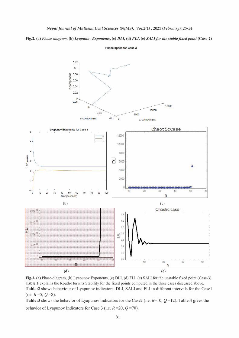
Fig.2. (a) Phase-diagram, (b) Lyapunov Exponents, (c) DLI, (d) FLI, (e) SALI for the stable fixed point (Case-2)

(a)

(b) (c)

(d) (e)

Fig.3. (a) Phase-diagram, (b) Lyapunov Exponents, (c) DLI, (d) FLI, (e) SALI for the unstable fixed point (Case-3) Table:1 explains the Routh-Hurwitz Stability for the fixed points computed in the three cases discussed above. Table:2 shows behaviour of Lyapunov indicators: DLI, SALI and FLI in different intervals for the Case1 (i.e. R =5, Q =8). Table:3 shows the behavior of Lyapunov Indicators for the Case2 (i.e. R=10, Q =12). Table:4 gives the

behavior of Lyapunov Indicators for Case 3 (i.e. R =20, Q =70).

Rashmi Bhardwaj & Aashima Bangia / Dynamical Indicator of Human Body’s Physical Endurance

30

(d) (e)

Fig.1. (a) Phase-diagram, (b) Lyapunov Exponents, (c) DLI, (d) FLI, (e) SALI for the stable fixed point (Case-1)

(a)

(b) (c)

(d) (e)

Nepal Journal of Mathematical Sciences (NJMS), Vol.2(1) , 2021 (February): 25-34

31

Fig.2. (a) Phase-diagram, (b) Lyapunov Exponents, (c) DLI, (d) FLI, (e) SALI for the stable fixed point (Case-2)

(a)

(b) (c)

(d) (e)

Fig.3. (a) Phase-diagram, (b) Lyapunov Exponents, (c) DLI, (d) FLI, (e) SALI for the unstable fixed point (Case-3) Table:1 explains the Routh-Hurwitz Stability for the fixed points computed in the three cases discussed above. Table:2 shows behaviour of Lyapunov indicators: DLI, SALI and FLI in different intervals for the Case1 (i.e. R =5, Q =8). Table:3 shows the behavior of Lyapunov Indicators for the Case2 (i.e. R=10, Q =12). Table:4 gives the

behavior of Lyapunov Indicators for Case 3 (i.e. R =20, Q =70).

Rashmi Bhardwaj & Aashima Bangia / Dynamical Indicator of Human Body’s Physical Endurance

32

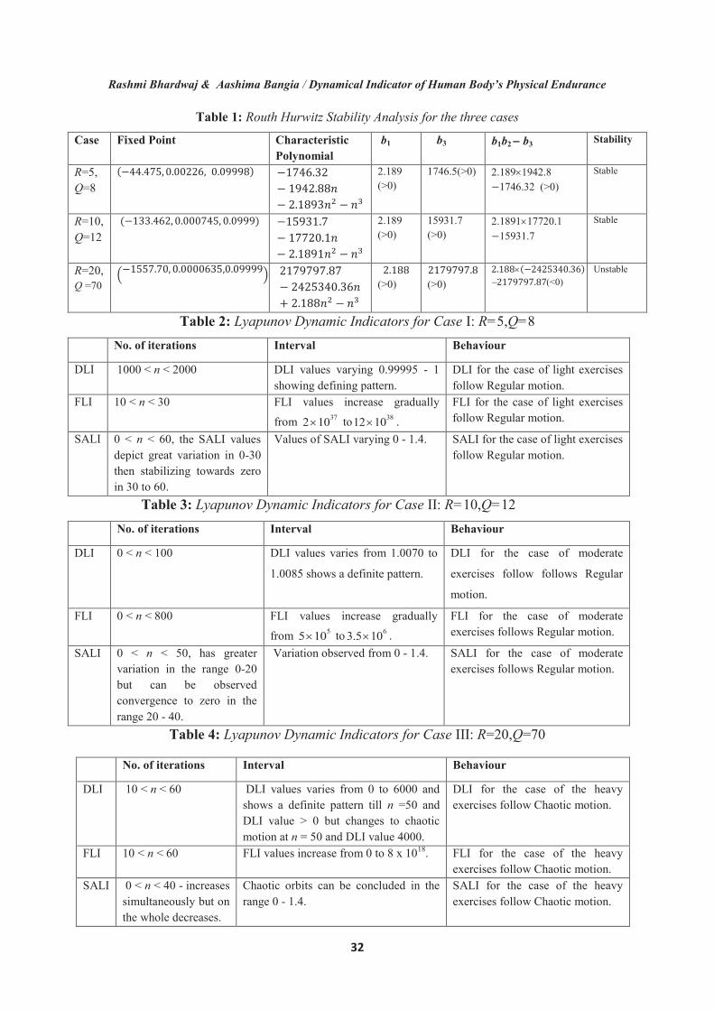
Table 1: Routh Hurwitz Stability Analysis for the three cases

Case Fixed Point Characteristic Polynomial

b1 b3 b1b2 b3 Stability

R=5, Q=8

( )

2.189 (>0)

1746.5(>0) 2.1891942.8 1746.32 (>0)

Stable

R=10, Q=12

( )

2.189 (>0)

15931.7 (>0)

2.189117720.1 15931.7

Stable

R=20, Q =70

( )

(>0)

(>0)

( ) (<0)

Unstable

Table 2: Lyapunov Dynamic Indicators for Case I: R=5,Q=8 No. of iterations Interval Behaviour

DLI 1000 < n < 2000 DLI values varying 0.99995 - 1 showing defining pattern.

DLI for the case of light exercises follow Regular motion.

FLI 10 < n < 30 FLI values increase gradually

from 372 10 to 3812 10 .

FLI for the case of light exercises follow Regular motion.

SALI 0 < n < 60, the SALI values depict great variation in 0-30 then stabilizing towards zero in 30 to 60.

Values of SALI varying 0 - 1.4. SALI for the case of light exercises follow Regular motion.

Table 3: Lyapunov Dynamic Indicators for Case II: R=10,Q=12 No. of iterations Interval Behaviour

DLI 0 < n < 100 DLI values varies from 1.0070 to

1.0085 shows a definite pattern.

DLI for the case of moderate

exercises follow follows Regular

motion.

FLI 0 < n < 800 FLI values increase gradually

from 55 10 to 63.5 10 .

FLI for the case of moderate exercises follows Regular motion.

SALI 0 < n < 50, has greater variation in the range 0-20 but can be observed convergence to zero in the range 20 - 40.

Variation observed from 0 - 1.4. SALI for the case of moderate exercises follows Regular motion.

Table 4: Lyapunov Dynamic Indicators for Case III: R=20,Q=70

No. of iterations Interval Behaviour

DLI 10 < n < 60 DLI values varies from 0 to 6000 and shows a definite pattern till n =50 and DLI value > 0 but changes to chaotic motion at n = 50 and DLI value 4000.

DLI for the case of the heavy exercises follow Chaotic motion.

FLI 10 < n < 60 FLI values increase from 0 to 8 x 1018. FLI for the case of the heavy exercises follow Chaotic motion.

SALI 0 < n < 40 - increases simultaneously but on the whole decreases.

Chaotic orbits can be concluded in the range 0 - 1.4.

SALI for the case of the heavy exercises follow Chaotic motion.

Nepal Journal of Mathematical Sciences (NJMS), Vol.2(1) , 2021 (February): 25-34

33

Conclusion

A mathematical model for levels of concentration of oxygen during various physical states of the human body like exercising, walking, jogging, resting etc. and two major components heart/ blood stream and the energy produced in the bodycells modeled as non-linearities factored into complex equations taken to be time dependent alongwith constant M. The stability analysis including the equilibrium points, Jacobian matrix, Eigen-system and its Phase space is estimated. Further, for improving accuracy and model efficiency, time-step analyzations also implemented. It is observed that there is a chaotic behavior in FLI, DLI and SALI graphs for the case where breath function, R and the amount of oxygen intake, Q are the highest, i.e. R=20 and Q=70. The time series graphs of amount of oxygen in physical state (x), amount of oxygen in heart (y) and amount of oxygen in the bodycells (z) variables indicate that on excessive exercising, oxygen supply/intake increases which further increases the oxygen concentration in heart and body cells. FLI’s increase for chaotic orbits for values of R = 20, Q =70 for the case of high intensity exercises and to linearly regular orbits for values of R = 5, Q = 8 and R = 10, Q =12 in the cases of light and moderate exercises respectively. SALI oscillating around a non-zero value for value of R=20, Q=70 while it tends to zero for values of R=5, Q=8 and R=10, Q=12. DLI’s the largest Eigen values form a definite pattern/curve for n=2000 for values of R=5, Q=8 and n =100 for R=10, Q=12 respectively as the motion is regular and distributed randomly as the motion is chaotic for n=60 and for R=20, Q=70. It is good to go for some kind of exercise on a daily basis. But, it is recommended to exercise for a limited time and period to avoid any harm to the body. It can be concluded that with various values of breath functions, R and the amount of oxygen intake, Q, concentration of oxygen varies. This means that more exercising leads to more of oxygen intake and further produces more energy which may keep us active, fresh and happy the whole day. In addition, excessive exercise will lead to excessive oxygen which may not be needed in the body and prove to be harmful. Acknowledgment Both of the authors are thankful towards G.G.S. Indraprastha University for facilitating research. Conflict of Interest: Authors declare no conflict of interest. References

[1]. Bhardwaj R. and Bangia A. (2016). Complex Dynamics of Meditating Body. Indian Journal of

Industrial and Applied Mathematics. 7(2): 106-116.

[2]. Bhardwaj R. (2016). Wavelets and fractal methods with Environmental Applications. Mathematical

Models, Methods and Applications. Eds: Siddiqi A.H., Manchanda P. and Bhardwaj R. 173-195.

[3]. Bhardwaj R., Kumar A., Maini P., Kar S.C. and Rathore L.S. (2007). Bias free rainfall forecast and

temperature trend based temperature forecast based upon T-170 model during monsoon season.

Meteorological Applications. 14(4) : 351-360.

[4]. Buckley J.P., Hedge A., Yates T., Copeland R.J., Loosemore M., Hamer M., Bradley G. and Dunstan

D.W. (2015). The sedentary office: A growing case for change towards better health and

productivity. British Journal of Sports Medicine. 49: 1357-1362.

[5]. Buman M.P., King A.C. (2010). Exercise as a Treatment to Enhance Sleep. American Journal of

Lifestyle Medicine. 4(6): 500-514.

Rashmi Bhardwaj & Aashima Bangia / Dynamical Indicator of Human Body’s Physical Endurance

32

Table 1: Routh Hurwitz Stability Analysis for the three cases

Case Fixed Point Characteristic Polynomial

b1 b3 b1b2 b3 Stability

R=5, Q=8

( )

2.189 (>0)

1746.5(>0) 2.1891942.8 1746.32 (>0)

Stable

R=10, Q=12

( )

2.189 (>0)

15931.7 (>0)

2.189117720.1 15931.7

Stable

R=20, Q =70

( )

(>0)

(>0)

( ) (<0)

Unstable

Table 2: Lyapunov Dynamic Indicators for Case I: R=5,Q=8 No. of iterations Interval Behaviour

DLI 1000 < n < 2000 DLI values varying 0.99995 - 1 showing defining pattern.

DLI for the case of light exercises follow Regular motion.

FLI 10 < n < 30 FLI values increase gradually

from 372 10 to 3812 10 .

FLI for the case of light exercises follow Regular motion.

SALI 0 < n < 60, the SALI values depict great variation in 0-30 then stabilizing towards zero in 30 to 60.

Values of SALI varying 0 - 1.4. SALI for the case of light exercises follow Regular motion.

Table 3: Lyapunov Dynamic Indicators for Case II: R=10,Q=12 No. of iterations Interval Behaviour

DLI 0 < n < 100 DLI values varies from 1.0070 to

1.0085 shows a definite pattern.

DLI for the case of moderate

exercises follow follows Regular

motion.

FLI 0 < n < 800 FLI values increase gradually

from 55 10 to 63.5 10 .

FLI for the case of moderate exercises follows Regular motion.

SALI 0 < n < 50, has greater variation in the range 0-20 but can be observed convergence to zero in the range 20 - 40.

Variation observed from 0 - 1.4. SALI for the case of moderate exercises follows Regular motion.

Table 4: Lyapunov Dynamic Indicators for Case III: R=20,Q=70

No. of iterations Interval Behaviour

DLI 10 < n < 60 DLI values varies from 0 to 6000 and shows a definite pattern till n =50 and DLI value > 0 but changes to chaotic motion at n = 50 and DLI value 4000.

DLI for the case of the heavy exercises follow Chaotic motion.

FLI 10 < n < 60 FLI values increase from 0 to 8 x 1018. FLI for the case of the heavy exercises follow Chaotic motion.

SALI 0 < n < 40 - increases simultaneously but on the whole decreases.

Chaotic orbits can be concluded in the range 0 - 1.4.

SALI for the case of the heavy exercises follow Chaotic motion.

Nepal Journal of Mathematical Sciences (NJMS), Vol.2(1) , 2021 (February): 25-34

33

Conclusion

A mathematical model for levels of concentration of oxygen during various physical states of the human body like exercising, walking, jogging, resting etc. and two major components heart/ blood stream and the energy produced in the bodycells modeled as non-linearities factored into complex equations taken to be time dependent alongwith constant M. The stability analysis including the equilibrium points, Jacobian matrix, Eigen-system and its Phase space is estimated. Further, for improving accuracy and model efficiency, time-step analyzations also implemented. It is observed that there is a chaotic behavior in FLI, DLI and SALI graphs for the case where breath function, R and the amount of oxygen intake, Q are the highest, i.e. R=20 and Q=70. The time series graphs of amount of oxygen in physical state (x), amount of oxygen in heart (y) and amount of oxygen in the bodycells (z) variables indicate that on excessive exercising, oxygen supply/intake increases which further increases the oxygen concentration in heart and body cells. FLI’s increase for chaotic orbits for values of R = 20, Q =70 for the case of high intensity exercises and to linearly regular orbits for values of R = 5, Q = 8 and R = 10, Q =12 in the cases of light and moderate exercises respectively. SALI oscillating around a non-zero value for value of R=20, Q=70 while it tends to zero for values of R=5, Q=8 and R=10, Q=12. DLI’s the largest Eigen values form a definite pattern/curve for n=2000 for values of R=5, Q=8 and n =100 for R=10, Q=12 respectively as the motion is regular and distributed randomly as the motion is chaotic for n=60 and for R=20, Q=70. It is good to go for some kind of exercise on a daily basis. But, it is recommended to exercise for a limited time and period to avoid any harm to the body. It can be concluded that with various values of breath functions, R and the amount of oxygen intake, Q, concentration of oxygen varies. This means that more exercising leads to more of oxygen intake and further produces more energy which may keep us active, fresh and happy the whole day. In addition, excessive exercise will lead to excessive oxygen which may not be needed in the body and prove to be harmful. Acknowledgment Both of the authors are thankful towards G.G.S. Indraprastha University for facilitating research. Conflict of Interest: Authors declare no conflict of interest. References

[1]. Bhardwaj R. and Bangia A. (2016). Complex Dynamics of Meditating Body. Indian Journal of

Industrial and Applied Mathematics. 7(2): 106-116.

[2]. Bhardwaj R. (2016). Wavelets and fractal methods with Environmental Applications. Mathematical

Models, Methods and Applications. Eds: Siddiqi A.H., Manchanda P. and Bhardwaj R. 173-195.

[3]. Bhardwaj R., Kumar A., Maini P., Kar S.C. and Rathore L.S. (2007). Bias free rainfall forecast and

temperature trend based temperature forecast based upon T-170 model during monsoon season.

Meteorological Applications. 14(4) : 351-360.

[4]. Buckley J.P., Hedge A., Yates T., Copeland R.J., Loosemore M., Hamer M., Bradley G. and Dunstan

D.W. (2015). The sedentary office: A growing case for change towards better health and

productivity. British Journal of Sports Medicine. 49: 1357-1362.

[5]. Buman M.P., King A.C. (2010). Exercise as a Treatment to Enhance Sleep. American Journal of

Lifestyle Medicine. 4(6): 500-514.

Rashmi Bhardwaj & Aashima Bangia / Dynamical Indicator of Human Body’s Physical Endurance

34

[6]. Buskirk R.V. and Jeffries C. (1985). Observation of chaotic dynamics of coupled non-linear

oscillator. Physical Review A. , 31(5): 3332-33357.

[7]. Dinas P.C., Koutedakis Y. and Flouris A.D. (2011). Effects of exercise and physical activity on

depression. Irish Journal of Medical Science. 180(2): 319-325.

[8]. Durai V.R. and Bhardwaj R. (2014). Location specific forecasting of maximum and minimum

temperature over India by using the statistical bias corrected output of global forecasting system.

Journal of Earth System Science. 123(5) : 1171-1195.

[9]. Durai V.R. and Bhardwaj R. (2014). Forecasting quantitative rainfall over India using Multi-Model

Ensemble Technique. Meteorology and Atmospheric Physics. 126(1-2) : 31-48.

[10]. Froeschle Cl. , Gonczi R. and Lega E. (1997). The Fast Lyapunov Indicator: A simple tool to detect

weak chaos. Application to the structure of the main a steroidal belt. Planetary and Space Science.

45(7): 881-886.

[11]. Grassberger P. and Procaccia I. (1983). Measuring the Strangeness of Strange Attractors. Physica D:

Nonlinear Phenomena. 9(1-2): 189-208.

[12]. Lega E.and Froesschle C. (2001). On the relationship between Fast Lyapunov Indicator and Periodic

orbit for symplectic mappings. Celestial Mechanics and Dynamical Astronomy. 81(1-2): 129-147.

[13]. Li D., Lu J.A.and Wu X. (2005). Linearly Coupled Synchronization of the Unified Chaotic Systems

and the Lorenz Systems. Chaos, Solitons & Fractals. 23(1): 79-85.

[14]. Martelli M. (2011). Introduction to Discrete Dynamical Systems and Chaos. John Wiley & Sons,

New York.

[15]. Nagashima H. and Baba Y. (2005). Introduction to Chaos: Physics and Mathematics of Chaotic

Phenomena. CRC Press, India.

[16]. Nikić P.K. (2010). Yoga-The Light of Micro-Universe. Proceedings of the International

Interdisciplinary Scientific Conference “Yoga In Science – Future And Perspectives”. Belgrade,

Serbia. pp. 156-161

[17]. Pimlott N. (2010). The miracle drug. Canadian Family physician Medecin de famille

Canadien. 56 (5): 407-409.

[18]. Saha L.M. and Budhraja M. (2007). The largest eigenvalue: An indicator of chaos. International

Journal of Applied Mathematics and Mechanics. 3(1): 61-71.

[19]. Saha L.M. , Das M.K. and Budhraja M. (2006). Characterization of attractors in Gumowski-Mira map using fast Lyapunov indicator. Forma. 21: 151-158. [20]. Skokos C., Antonopoulos C.G., Bountis T. and Vrahatis M.N. (2004). Detecting order and chaos in Hamiltonian systems by SALI method. Journal of Physics A: Mathematical and General. 37(24): 6269-6284. [21]. Skokos C. (2001). Alignment indices: A new, simple method for determining the ordered or chaotic

nature of orbits. Journal of Physics A: Mathematical and General. 34(47) : 10029-10043.

Nepal Journal of Mathematical Sciences (NJMS) Vol. 2(1), 2021 (February): 35-42 ISSN: 2738-9928 (online), 2738-9812 (print) School of Mathematical Sciences, Tribhuvan University, Kathmandu, Nepal

Research Article Received Date: October 15, 2020 Accepted Date: December 20, 2020 Published Date: February 5, 2020

35

On Generalized Recurrent Finsler Connection Khageshwar Mandal

Department of Mathematics,

Padma Kanya Campus, Tribhuvan University, Kathmandu, Nepal

Email: khageshwarmandal@gmail.com Abstract: The purpose of the present paper is to generalize the concept of recurrent Finsler connection by taking -

connection by applying -covariant derivative of as recurrent. Such a connection will be called a

generalized -recurrent Finsler connection. The relation between curvature tensors of Cartan's

connection and generalized -recurrent Finsler connection has been established.

Keywords: Finsler connection, Cartan's connection, Curvature tensor, Torsion tensor, Deflection tensor.

1. Introduction Cartan (Cartan,1994) published his monograph 'les espaces de Finsler' and fixed his method to

determine a notion of connection in the Geometry of Finsler space. Matsumoto (Matsumoto, 2008) determined uniquely the Cartan's connection CT by following conditions: (1) the connection is metrical; (2) the deflection tensor field vanishes; (3) the torsion tensor field T vanishes; (4) the torsion tensor field S vanishes.

Hozo (Hojo, 2016, Hashiguchi, 1998) introduced the connections, which depend on a real parameter P and make v-covariant derivative

zero just like as in case

of . The cartan's connection is really the case when P takes its value two and so the connection determined by Hozo is a generalization of .

Recently Prasad and Srivastava (2012) have introduced a recurrent Finsler connection which is neither -metricalnor v-metrical, but is is recurrent with respect to both -and v-covariant, derivatives. Suh a Finsler connection has been called an hv-recurrent Finsler connection.

To avoid confusions, we use - and v-covariant derivatives with respect to Cartan's connection by while these covariant derivatives with respect to generalized -recurrent Finsler connection will be denoted by ǁ k and ǁ k respectively.

The quantities corresponding to generalized -recurrent Finsler connection will be denoted by putting p on the top of the quantity followed by putting (a) in front of the quantity, while the quantities corresponding to Cartan's connection will be denoted as usual.

We have not used the raising and lowering of indices of objects, but if anywhere necessary, the metric will be used.