dynamic system models for optimal control - syscop.de · i in this course, treatdeterministic di...

Dynamic Systems and Optimal Control

I “Optimal control” = optimal choice of inputs for adynamic system

I What type of dynamic system?I Stochastic or deterministic?I Discrete or continuous time?I Discrete or continuous states?

I In this course, treat deterministic differential equations anddiscrete time systems

Continous and discrete time deterministic systems

I Continuous time Ordinary Differential Equation (ODE):

x(t) = f (x(t), u(t)), t ∈ [0,T ]

states x ∈ Rnx , control inputs u ∈ Rnu , f : Rnx × Rnu → Rnx ,

I Discrete time systems:

xk+1 = f (xk , uk), k = 0, 1, . . .

states xk ∈ X , control inputs uk ∈ U. Sets X ,U can becontinuous or discrete.

(Some other dynamic system classes)

I Games like chess: discrete time and state (chess figurepositions), adverse player exists.

I Robust optimal control: like chess, but continuous time andstate (adverse player exists in form of worst-case disturbances)

I Control of Markov chains: discrete time, system described bytransition probabilities

P(xk+1|xk , uk), k = 0, 1, . . .

I Stochastic Optimal Control of ODE: like Markov chain, butcontinuous time and state

Ordinary Differential Equations (ODE)

System dynamics can be manipulated by controls and parameters:

x(t) = f (t, x(t), u(t), p)

• simulation interval: [t0, tend]

• time t ∈ [t0, tend]

• state x(t) ∈ Rnx

• controls u(t) ∈ Rnu ←− manipulated

• design parameters p ∈ Rnp ←− manipulated

ODE Example: Dual Line Kite Model

I Kite position relative to pilot in sphericalpolar coordinates r , φ, θ. Line length rfixed.

I System states are x = (θ, φ, θ, φ).

I We can control roll angle u = ψ.

I Nonlinear dynamic equations:

θ =Fθ(θ, φ, θ; φ, ψ)

rm+ sin(θ) cos(θ)φ2

φ =Fφ(θ, φ, θ; φ, ψ)

rm sin(θ)− 2 cot(θ)φθ

I Summarize equations as x = f (x , u).

Initial Value Problems (IVP)

THEOREM [Picard 1890, Lindelof 1894]:

Initial value problem in ODE

x(t) = f (t, x(t), u(t), p), t ∈ [t0, tend],

x(t0) = x0

I with given initial state x0, design parameters p, and controlsu(t),

I and Lipschitz continuous f (t, x , u(t), p)

has unique solution

x(t), t ∈ [t0, tend]

NOTE: Existence but not uniqueness guaranteed iff (t, x , u(t), p) only continuous [G. Peano, 1858-1932].Non-uniqueness example: x =

√|x |

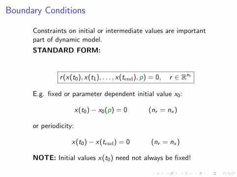
Boundary Conditions

Constraints on initial or intermediate values are importantpart of dynamic model.

STANDARD FORM:

r(x(t0), x(t1), . . . , x(tend), p) = 0, r ∈ Rnr

E.g. fixed or parameter dependent initial value x0:

x(t0)− x0(p) = 0 (nr = nx)

or periodicity:

x(t0)− x(tend) = 0 (nr = nx)

NOTE: Initial values x(t0) need not always be fixed!

Kite Example: Periodic Solution Desired

I Formulate periodicity asconstraint.

I Leave x(0) free.

I Minimize integrated powerper cycle

minx(·),u(·)

∫ T

0L(x(t), u(t))dt

subject to

x(0)− x(T ) = 0

x(t)− f (x(t), u(t)) = 0, t ∈ [0,T ].

Objective Function Types

Typically, distinguish between

I Lagrange term (cost integral, e.g. integrated deviation):∫ T

0L(t, x(t), u(t), p)dt

I Mayer term (at end of horizon, e.g. maximum amount ofproduct):

E (T , x(T ), p)

I Combination of both is called Bolza objective.

Differential-Algebraic Equations (DAE) - Semi-Explicit

Augment ODE by algebraic equations g and algebraicstates z

x(t) = f (t, x(t), z(t), u(t), p)0 = g(t, x(t), z(t), u(t), p)

• differential states x(t) ∈ Rnx

• algebraic states z(t) ∈ Rnz

• algebraic equations g(·) ∈ Rnz

Standard case: index one ⇔ matrix ∂g∂z ∈ Rnz×nz invertible.

Existence and uniqueness of initial value problems similar asfor ODE.

Tutorial DAE Example

Regard x ∈ R and z ∈ R, described by the DAE

x(t) = x(t) + z(t)0 = exp(z)− x

I Here, one could easily eliminate z(t) by z = log x , to get theODE

x(t) = x(t) + log(x(t))

Tutorial DAE Example

Regard x ∈ R and z ∈ R, described by the DAE

x(t) = x(t) + z(t)0 = exp(z)− x + z

I Now, z cannot be eliminated as easily as before, but still, theDAE is well defined because ∂g

∂z (x , z) = exp(z) + 1 is alwayspositive and thus invertible.

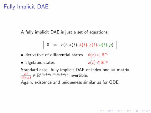
Fully Implicit DAE

A fully implicit DAE is just a set of equations:

0 = f (t, x(t), x(t), z(t), u(t), p)

• derivative of differential states x(t) ∈ Rnx

• algebraic states z(t) ∈ Rnz

Standard case: fully implicit DAE of index one ⇔ matrix∂f

∂(x ,z) ∈ R(nx+nz )×(nx+nz ) invertible.

Again, existence and uniqueness similar as for ODE.

Multi Stage Processes

Two dynamic stages can be connected by a discontinuous“transition”. E.g. Intermediate Fill Up in Batch Distillation

��

��

�� ···

···

��6?

6

��

��

�� ···

···

��6?

6

dynamic stage 0

6

Volume

transitionx1(t1) = ftr(x0(t1), p)

?

x0(t) x1(t)

t1

-timedynamic stage 1

Multi Stage Processes II

Also different dynamic systems can be coupled. E.g. batchreactor followed by distillation (different state dimensions)

'

&

$

%��

A + B → C ��

��

�� ···

···

��6?

6

dynamic stage 0

6 6

transitionx1(t1) = ftr(x0(t1), p)

x0(t)

x1(t)

t1

-timedynamic stage 1

Partial Differential Equations

I Instationary partial differential equations (PDE) arise e.g intransport processes, wave propagation, ...

I Also called “distributed parameter systems”

I Often PDE of subsystems are coupled with each other (e.g.flow connections)

I Method of Lines (MOL): discretize PDE in space to yieldODE or DAE system.

I Often MOL can be interpreted in terms of compartmentmodels.

From continous ODE to discrete time systems

I Solution x(t) of ODE x = f (x , u) can be computed bynumerical integration (details in talk by Rien)

I if control is kept constant u(t) ≡ q and initial value x(0) = sspecified, integrator delivers solution trajectory

x(t; s, q)

I for sampling time ∆t, can use fd(s, q) := x(∆t; s, q) toobtain discrete time system

sk+1 = fd(sk , qk)

I In case of linear ODE x = Ax + Bu, discrete linear systemsk+1 = Adsk + Bdq can be obtained by matrix exponentials:

Ad := eA∆t , Bd :=

∫ ∆t

0eAtBdt

Linearization of Nonlinear Systems

I Nonlinear discrete time system fd(s, q) can be linearized atany point (s, q) to obtain first order Taylor expansion:

fd(s, q) ≈ fd(s, q) +∂fd∂s

(s, q)︸︷︷︸=:Ad

(s − s) +∂fd∂q

(s, q)︸︷︷︸=:Bd

(q − q)

I If evaluated at steady state, derivatives are identical to matrixexponentials of linearized continous time system (matter ofconvenience which way to go).

Linear Quadratic Regulator (LQR)

Simplest optimal control problem: linear system xk+1 = Axk + Bukwith quadratic cost on infinite horizon:

minu0,x1,u1,...

∞∑k=0

x>k Qxk + u>k Ruk

I Solved with help of discrete time Riccati equation

P = Q + ATPA− (ATPB)(R + BTPB)−1(BTPA)

to determine matrix P yielding optimal feedback control

u∗(x) = − (R + BTPB)−1(BTPA)︸︷︷︸=K

x

I Implemented e.g. in MATLAB’s dlqr command.

Summary

Dynamic models for optimal control consist ofI differential equations (ODE/DAE/PDE)I boundary conditions, e.g. initial/final values, periodicityI objective in Lagrange and/or Mayer formI transition stages in case of multi stage processes

PDE can be transformed to DAE by Method of Lines (MOL)

ODE standard form for this course:

x(t) = f (x(t), u(t))

I Discrete time models can be obtained by numerical integration

I Linear quadratic regulator (LQR) can easily be computed forlinearized systems

References

I K.E. Brenan, S.L. Campbell, and L.R. Petzold: The NumericalSolution of Initial Value Problems in Differential-AlgebraicEquations, SIAM Classics Series, 1996.

I U.M. Ascher and L.R. Petzold: Computer Methods forOrdinary Differential Equations and Differential-AlgebraicEquations. SIAM, 1998.

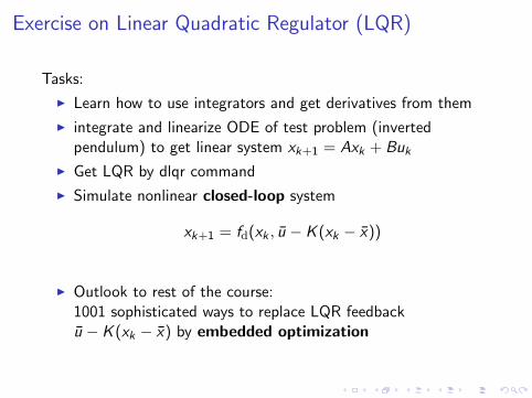
Exercise on Linear Quadratic Regulator (LQR)

Tasks:

I Learn how to use integrators and get derivatives from them

I integrate and linearize ODE of test problem (invertedpendulum) to get linear system xk+1 = Axk + Buk

I Get LQR by dlqr command

I Simulate nonlinear closed-loop system

xk+1 = fd(xk , u − K (xk − x))

I Outlook to rest of the course:1001 sophisticated ways to replace LQR feedbacku − K (xk − x) by embedded optimization

dynamic system models for optimal control - syscop.de · i in this course, treatdeterministic di...

Documents