dynamic stress concentration in a single particle
TRANSCRIPT

DYNAMIC STRESS CONCENTRATION IN A SINGLE
PARTICLE COMPOSITE
Sinisa Bugarin A thesis submitted to the Faculty of Engineering and the Built Environment, University of the Witwatersrand, Johannesburg, in fulfilment of the requirements for the degree of Doctor of Philosophy. Johannesburg, 2012

1
Abstract
The fracture and fatigue properties of particle reinforced matrix composites are greatly
influenced by stress concentration around the reinforcements as the failure of a structural
member often initiates at regions of high stress concentration. Determining stress
concentration has been the focus of number of researchers for quite some time in order
to better understand the failure mechanics of structural members. The first part of the
study investigates the stress concentration around a spheroidal particle that is embedded in a
large elastic matrix and subjected to dynamic loading. Interaction between neighboring
particles is ignored. The results are therefore valid for composites with low volume fractions.
The problem is studied by extending a hybrid technique that was previously developed for
axisymmetric loading. In the hybrid technique, a fictitious spherical boundary enclosing the
particle is drawn. The fictitious boundary divides the entire region into interior and exterior
regions. The interior region is modeled through an assemblage of conventional finite
elements while the exterior region is represented by spherical wave functions. Coupling of
the solutions for the interior and exterior regions is achieved by imposing the continuity of
displacements and tractions along the common boundary B. This leads to a set of linear
equations that enables the displacements and stresses at any point to be determined. It is
found that the stress concentrations within the matrix at the matrix-particle interface are
dependent on the frequency of the dynamic excitation, aspect ratio of the particle and the
material properties of both matrix and a particle. The study reveals that the dynamic stress
concentration can reach much higher values than the static case.
A second part of the study involved investigating the potential of using an interphase layer to
reduce stress concentrations under a dynamic loading in Mg matrix surrounding a SiC
particle. An interphase layer was applied between the particle and the matrix and the contact
between them was assumed to be perfect. Both constant property materials and functionally
graded materials were considered for the interphase. A constant property interphase was
modelled as a single layer while a functionally graded interphase was divided into a number
of sublayers and each sublayer was treated as having constant material properties. Numerical
results reveal that the interphase layer made of a constant property material shows better
stress concentration reduction than that made of functionally graded materials. An interphase
layer with low values of both shear modulus and Poisson's ratio is necessary for a significant
stress concentration reduction. Studies were focused on reducing the concentration that
occurs over a range of frequencies.
The third part of the study investigates the size effects as the particle size reduces to
nanometers. This part of the study was inspired by the current interest in nanomaterials. For
instance, a quantum dot that is embedded in the matrix of a composite could introduce stress
concentrations under dynamic loading. This is studied here by using the surface/interface
theory of elasticity. It is found that the stress concentration values are significantly
dependent on the elastic properties of the surface/interface and the frequency of excitation.

2
The work presented here has resulted in three publications in international journals and three
conference presentations. The complete list is given below:
1. R. Paskaramoorthy, S. Bugarin and R. Reid: Effect of an interphase layer on the dynamic
stress concentration in a Mg-matrix surrounding a SiC-particle. Journal of Composite and
Structures, 2009, 91, 451–460.
2. R. Paskaramoorthy, S. Bugarin and R. Reid. Analysis of stress concentration around a
spheroidal cavity under asymmetric dynamic loading. Journal of Solids and Structures,
July 2011, 48, Issues 14-15, 2255-2263.
3. S. Bugarin, R. Paskaramoorthy and R. Reid. Influence of the geometry and material
properties on the dynamic stress field in the matrix containing a spheroidal particle
reinforcement. Composite Part B: Engineering, Volume 43, Issue 2, March 2012, Pages
272-279
4. Paskaramoorthy R, Bugarin S, Reid RG. A hybrid finite element method for stress concentration in a single fibre composite. ASME 2011 Applied Mechanics and Materials
Conference in Chicago, Illinois, USA, June 2011.
5. Bugarin S, Paskaramoorthy R, Reid RG. A hybrid finite element method for stress analysis around an inhomogeneity under dynamic loads. South African Conference on
Applied Mechanics, 2010, University of Pretoria, South Africa.
6. Paskaramoorthy R, Bugarin S, Reid RG. On the reduction of dynamic stress concentrations in a SiC/Mg composite using interphase layers. Proceedings of the Sixth
International Conference on Composite Science and Technology, Durban, January 2007.
(ISBN: 1-86840-642-3)

3
Declaration
I declare that this thesis is entirely my own work. It is being submitted for the degree of
Doctor of Philosophy in the University of The Witwatersrand, Johannesburg. It has not been
submitted before for any degree or examination in any other University.
_____________________________________
(Signature of candidate)
_________day of___________ 2012

4
Acknowledgments
I would like to thank my supervisor Professor R. Paskaramoorthy, for his assistance in
guiding me into the world of scientific research. Many thanks also go to National Aerospace
Centre of Excellence in Strong Materials for bursary support during this research study. To
my colleagues Kmil Midor, Andrew Allcock, Nico Wilke and Adolph Vogel I extend my
gratitude for help and advice with Matlab and Python programming.
5
Table of Contents
Abstract ...................................................................................................................................... 1 Declaration ................................................................................................................................. 3 Acknowledgments...................................................................................................................... 4 Table of Contents ....................................................................................................................... 5 List of Figures ............................................................................................................................ 7 Glossary of terms ....................................................................................................................... 9 1. Introduction ..................................................................................................................... 10
1.1. Introduction to Composites .......................................................................................... 10 1.2. Introduction to metal-matrix composites ..................................................................... 12 1.3. Failure and mechanisms of crack initiation in PRMMCs ............................................ 18 1.4. Interphase layer effects ................................................................................................ 20 1.4. Surface/interface effects at nano-scale ......................................................................... 22
2. General problem and fundamental equations ................................................................. 24 2.1. Statement of the problem ............................................................................................ 24
3. Stress concentration in matrix around spheroidal particle .............................................. 29 under asymmetric dynamic loading ......................................................................................... 29
3.1. Formulation of the problem ........................................................................................ 31 3.1.1. Interior region ......................................................................................................... 31
3.1.2. Exterior region ........................................................................................................ 33
3.1.3. Incident waves ........................................................................................................ 33
3.1.4. Scattered waves .................................................................................................. 35
3.2. Global Solution ........................................................................................................... 38 3.3. Numerical results and discussion ............................................................................ 39 3.4. Conclusion .................................................................................................................. 49
4. Effect of an interphase layer on the dynamic stress concentration in a .......................... 50 Mg matrix surrounding a SiC particle ..................................................................................... 50
4.1. Formulation of the Problem ......................................................................................... 50 4.1.2. Refracted wave field in the interphase layer .......................................................... 53
4.1.3. Incident and scattered wave fields in the matrix .................................................... 54
4.1.4. Boundary conditions ............................................................................................... 56
4.2. Numerical results and discussion ................................................................................. 57 4.2.1. Effect of an interphase layer of higher elastic modulus than the matrix ................ 61
4.2.2. Effect of a functionally graded interphase layer ..................................................... 62
4.2.3. Effect of an interphase layer with an elastic modulus lower than the matrix ......... 64
4.2.4. Effect of Poisson’s ratio ......................................................................................... 65
4.2.5. Effect of Density ..................................................................................................... 66
4.3. Conclusion ................................................................................................................... 67 5. Surface effects on the dynamic elastic state surrounding a ............................................. 68 nanosized spherical particle ..................................................................................................... 68
5.1. Problem Formulation ................................................................................................... 68 5.1.1. Refracted waves in the particle ........................................................................ 71

6
5.1.2. Surface/interface elasticity ................................................................................ 71
5.2. Numerical results and discussion ........................................................................... 74 5.3. Conclusion .................................................................................................................. 82
6. Summary and final conclusion......................................................................................... 83 References ................................................................................................................................ 85 Appendix A .............................................................................................................................. 89 Appendix B .............................................................................................................................. 90 Appendix C .............................................................................................................................. 95 Appendix D .............................................................................................................................. 96

7
List of Figures
Figure 1.1 Schematic showing the three main types of composite [1] .................................... 11
Figure 1.2 Mid-fuselage structure of Space Shuttle Orbiter showing boron-aluminum tubes [2]. ............................................................................................................................................ 14
Figure 1.3 Properties of AMCs versus conventional alloys [3] ............................................... 16
Figure 2.1 Schematic illustration of the general problem. ....................................................... 24
Figure 3.1 Problem geometry with cylindrical and spherical coordinate systems. ........... 30
Figure 3.2 Finite element mesh of the interior region for b/a = 3. ..................................... 32
Figure 3.3 Comparison of stress concentration values along the circumference of a spherical particle for ω*= 0.01(ρ*=1, µ*=8, ν1= ν2=0.3) ....................................................... 41
Figure 3.4 Comparison of stress concentration values along the circumference of a spherical particle for ω*= 3 (ρ*=1, µ*=8, ν1= ν2=0.3) ........................................................... 41
Figure 3.5 Comparison of stresses along the circumference of a spheroidal particle of b/a=3 subject to static loading ............................................................................................... 43
Figure 3.6 Comparison of stresses along the circumference of a spheroidal particle of b/a=5 subject to static loading ............................................................................................... 43
Figure 3.7 Angular distribution of stress concentration on the particle matrix interface for b/a=1 (ρ*=1, µ*=8, ν1= ν2=0.3) ............................................................................................... 45
Figure 3.8 Angular distribution of stress concentration on the particle matrix interface for b/a=3 (ρ*=1, µ*=8, ν1= ν2=0.3) ............................................................................................... 46
Figure 3.9 Angular distribution of stress concentration on the particle matrix interface for b/a =5 (ρ*=1, µ*=8, ν1= ν2=0.3) .............................................................................................. 47
Figure 3.11 Effect of particle stiffness on peak stress concentration values for: 3.17a) .... 48
b/a =1 and 3.17b) b/a =5 (ρ*=1, ν1= ν2=0.3) ......................................................................... 48
Figure 3.12 Effect of particle density on peak peak stress concentration values for b/a =5 (µ*=8, ν1=ν2=0.3) .................................................................................................................... 49
Figure 4.1 Schematic illustration of the matrix-interphase-particle problem. ......................... 51
Figure 4.2 Stress distribution around the particle without the interphase layer for two frequencies (µ2 / µ1 = 11.4; ν2 = ν1 = 0.3).................................................................................. 60
Figure 4.3 Effect of interphase layer with an elastic modulus larger than that of the matrix .. 61
Figure 4.4 Schematic variation of the elastic modulus of a functionally graded material ....... 63
Figure 4.5 Effect of a functionally graded interphase layer ..................................................... 63
Figure 4.6 Effect of interphase layer with a stiffness lower than that of the matrix ................ 64
Figure 4.7 Effect of Poisson’s ratio of the interphase on the stress concentration .................. 65
Figure 4.8 Angular location of maximum von Mises stress for different Poisson’s ratios (µ3 / µ1 = 0.4, ρ3 / ρ1 =1) .................................................................................................................. 66
Figure 4.9 Effect of density of interphase layer on maximum von Mises stress (µ3 / µ1 = 0.4, ν3 = 0.1, ν2 = ν1 = 0.3) ............................................................................................................... 66
Figure 5.1 Schematic illustration of the general problem. ....................................................... 68
Figure 5.1 Angular distribution of stress concentration in the matrix at the nano-particle matrix interface for ω*= 0.1 (ρ*=1, µ*=8, ν1= ν2=0.3) .......................................................... 77
Figure 5.2 Angular distribution of stress concentration in the matrix at the nano-particle matrix interface for ω*= 3 (ρ*=1, µ*=8, ν1= ν2=0.3) .............................................................. 78
Figure 5.3 Radial distribution of stress concentration in the matrix at θ π = 0.75 angle for
ω*= 0.1 (ρ*=1, µ*=8, ν1= ν2=0.3) ............................................................................................ 79
Figure 5.4 Radial distribution of stress concentration in the matrix at θ π = 0.75 angle for
ω*= 2 (ρ*=1, µ*=8, ν1= ν2=0.3) ............................................................................................... 79
Figure 5.5 Effect of k2 on the peak stress concentration values in the matrix at the nano-particle matrix interface (ρ*=1, µ*=8, ν1= ν2=0.3) ................................................................. 80

8
Figure 5.6 Effect of nano-particle/matrix stiffness ratio µ* on the peak stress concentration values in the matrix at the particle matrix interface for k2 =0.5 (ρ*=1, ν1= ν2=0.3) ............ 81
Figure 5.7 Effect of nano-particle/matrix stiffness ratio µ* on the peak stress concentration values in the matrix at the particle matrix interface for k2 =2 (ρ*=1, ν1= ν2=0.3) ............... 82
Figure C.1. Finite element mesh for the spheroidal particle (b/a=3) for static loading case.................................................................................................................................................. 95
Figure C.2. Finite element mesh for the spheroidal particle (b/a=5) for static loading case.................................................................................................................................................. 95

9
Glossary of terms
U - displacement vector
xxσ - normal stress in Cartesian coordinate system
xyσ - shear stress in Cartesian coordinate system
xxε - normal strain in Cartesian coordinate system
xyε - shear strain in Cartesian coordinate system
RRσ - normal stress in Spherical coordinate system
Rθσ - shear stress in Spherical coordinate system
RRε - normal strain in Spherical coordinate system
Rθε - shear strain in Spherical coordinate system
R - radial distance from the centre of inhomogeneity in Spherical coordinates system
r - radial distance from the centre of inhomogeneity in Cylindrical coordinates system
a - dimension of the inclusion along the x axis
b - dimension of the inclusion along the z axis
θ - angle in zx-plane
φ - angle in xy-plane
t - time variable
λ - Lamé constant of the material
µ - Lamé constant of the medium
ν - Poisson’s ratio of the medium
ρ - density of the medium
ω - frequency of the incident wave
ω* - normalized frequency of the incident wave
α - wave number
β - wave number
nj - Spherical Bessel function of the first kind
ny - Spherical Bessel function of the second kind
mnP - Legendre polynomial
( )1nh - Henkel function of the first kind
( )2nh - Henkel function of the second kind
χ - Pressure wave potential function
ϕ - Shear wave potential function
ψ - Shear wave potential function

10
1. Introduction
1.1. Introduction to Composites
A composite material is a microscopic combination of two or more distinct materials, having
a recognizable interface between them, which have been bonded together at a scale that is
sufficiently fine that the result can be considered a material with properties of its own.
Composites are engineered materials that have been designed to provide higher structural
efficiency, which is higher specific strength and specific stiffness relative to previously
available materials. High strength and modulus of elasticity of reinforcements provide
strength and stiffness in composites. By selecting the reinforcements with desired levels of
strength and stiffness and by controlling the volume fraction of reinforcements the actual
magnitude of composite strength and stiffness can be controlled. Composites are used not
only for their structural properties, but also for their thermal, electrical and environmental
applications. Modern composites are usually optimized to achieve a particular balance of
properties for a given range of applications. The composite material has a balance of
structural properties that is superior to either constituent material alone. The improved
structural properties generally result from a load-sharing mechanism.
Composites typically have a fibre or particle phase that is stiffer than the continuous matrix
phase. The distinction of the matrix in composite from other two or more phase alloys comes
about from the processing of the composite. This is possible by the virtue of the fact that the
melting temperature of the matrix is much lower than that of the reinforcement and the two
can be mixed together to distinguish a composite from two or more phase alloys. Many types
of reinforcements often have good thermal and electrical conductivity, good wear resistance
and a coefficient of thermal expansion (CTE) that is less than the matrix. Composites are
commonly classified at two distinct levels. The first classification is usually made with
respect to the matrix constituent of which major composite classes include organic-matrix
composites (OMCs), metal-matrix composites (MMCs) and ceramic-matrix composites
(CMCs). In each of these composites the matrix is typically a continuous phase throughout
the component. The second level of classification refers to the reinforcement form being
particulate-reinforcement, whisker reinforcement, continuous fibre reinforcement (see Figure
1.1) and woven fibre composites (braided and knitted fibre architectures). The reinforcement
volume fraction must generally be substantial (10% or more) to provide a useful increase in
properties.

11
Figure 1.1 Schematic showing the three main types of composite [1]
Particulate-reinforcements and whisker reinforcement are classified as “discontinuous”
reinforcements as the reinforcing phase is discontinuous for the lower volume fraction (20% -
30%) typically used in MMCs. In particle reinforcement all of particle’s dimensions are
roughly equal and thus, particle-reinforced composites include those reinforced by spheres,
flakes and many other shapes of roughly equal axes. Whisker reinforcements, with an aspect
ratio typically between 20 to a 100 are often considered together with particulates in MMCs.
Continuous fibre-reinforced composites contain reinforcements that have length much greater
than their cross-sectional dimensions and their length is comparable to the overall dimensions
of the composite part. The prime role of the fibers is to carry the load, while the matrix serves
to transfer and distribute the load to the fibers.
In fibre-reinforced composites, the strength and stiffness can also be controlled by specifying
the fibre direction. Highest structural efficiency is obtained when fibres are aligned along the
primary loading direction within the composites, which provides part of the motivation for
the widespread use of these materials. Simultaneously this fibre orientation produces a
material with lower structural efficiency for the loads perpendicular to the fibre direction.
These highly anisotropic properties must be considered in the use of such materials.
The purpose of the matrix is to bind the reinforcements together by virtue of its cohesive and
adhesive characteristics, to transfer the load to and between reinforcements, and to protect the
reinforcements from environmental handling. The matrix also provides a solid form to the
composite that aids in handling of the finished part in manufacture. In discontinuously
reinforced composites the matrix is particularly necessary as the reinforcements are not of
sufficient length to provide manageable form. The matrix is often a “weak link” from a
structural perspective in the composite since the reinforcements are typically stronger and
stiffer. However the matrix allows the strength of reinforcements to be used to their full
potential by holding reinforcing fibres in the proper orientation and position so that they can
carry the intended loads and distribute the loads more or less evenly among reinforcements.
A great deal of flexibility exists in the lay-up of composite. The fraction of fibres in any
given direction can be tailored in proportion to the load that must be supported thereby
significantly increasing structural efficiency of the composite. Some OMCs such as quasi-
isotropic graphite/epoxy laminate provide in-plane isotropy as required in some applications.

12
The specific stiffness of quasi-isotropic laminated OMCs is significantly higher than
structural metals, with the exception of few specialty titanium alloys and high strength steel.
Almost all high strength or high stiffness materials fail due to propagation of flaws under
loading. A fibre of such a material is inherently stronger than the bulk form as the size of the
flaw is limited by the small diameter of the fibre. If equal volumes of fibrous and bulk
material are compared, the flaw that would produce the failure in fibres will not propagate to
fail the entire assemblage of fibres, as would happen in the bulk material.
The technology base for fibre-reinforced MMCs is less established. Their use is limited due
to factors such as high cost of constituent material and processing difficulties of
monofilament-reinforced metal alloys. Cross-plied architectures have never been successfully
demonstrated in any commercial fibre-reinforced MMC. One of the few commercially
available is aluminium alloy reinforced with tow-based alumina (Al2O3) reinforcement which
is significantly cheaper than the graphite/epoxy OMC. The applications of fibre-reinforced
MMCs are limited to areas where metal-like behavior is important, including good wear
resistance, elevated temperature operation, high electrical conductivity and high bearing
strength.
Particle-reinforced metals provide essentially isotropic properties that are in the same general
range as graphite/epoxy quasi-isotropic material. Discontinuously reinforced aluminium
(DRA) is by far the most widely used MMC and a number of important applications have
been established. For reinforcement volume fraction less than 25%, DRA has good fracture
toughness and ductility, and structural efficiency that overlap that of quasi-isotropic organic
matrix composites (OMC). For higher volume fraction the fracture properties are lower, but
these materials are used widely for wear resistant applications, thermal management and
electronic packaging. The relatively low cost and ease of manufacturing makes DRA an
affordable material where high structural efficiency is required. Discontinuously reinforced
titanium (DRTi) is less established than DRA, but already has important applications,
including intake and exhaust valves in production automobile engines. Current DRTi
materials provide a balance of specific strength and specific stiffness that is superior to any
isotropic engineering material, including quasi-isotropic OMCs.
1.2. Introduction to metal-matrix composites
Metal Matrix Composites (MMCs) are composed of a metal matrix and a reinforcement, or
filler material, which confers excellent mechanical performance, and can be classified
according to whether the reinforcement is continuous (monofilament or multifilament) or
discontinuous (particle, whisker, short fibre or other). The principal matrix materials for
MMCs are aluminium and its alloys. To a lesser extent, magnesium and titanium are also
used, and for several specialised applications a copper, zinc or lead matrix may be employed.
The reinforcements can be metallic or ceramic (in general an oxide, a carbide or a nitride)

13
having much higher melting temperature than the matrix which allows mixing of the two
distinct materials together to form a composite. MMCs with discontinuous reinforcements are
usually less expensive to produce than continuous fibre reinforced MMCs, although this
benefit is normally offset by their inferior mechanical properties. Consequently, continuous
fibre reinforced MMCs are generally accepted as offering the ultimate in terms of mechanical
properties and commercial potential.
The first focused effort to develop metal-matrix composites (MMC) originated in the early
1950s and 1960s. Historically, MMCs, such as steel-wire reinforced copper, were among the
first continuous-fiber reinforced composites studied as a model system. Initial work in late
1960s was stimulated by the high-performance needs of the aerospace industry. In these
development efforts, performance, not cost, was the primary driver. The principal motivation
was to dramatically extend the structural efficiency of metallic materials while still retaining
the already utilized advantages such as high shear strength, high chemical inertness and
property retention at high temperatures. Boron filament, the first high-strength, high-modulus
reinforcement, was developed both for metal- and organic- matrix composites. Because of the
fiber-strength degradation and poor wettability in molten-aluminum alloys, the early carbon
fibers could only be properly reinforced in organic-matrix composites. Therefore, the
development of MMCs was primarily directed toward diffusion-bonding processing. At the
same time, optimum (air stable) surface coatings were developed for boron and graphite
fibers to facilitate wetting and inhibit reaction with aluminum or magnesium alloys during
processing.
Early work on sintered aluminium powder was an initiator to discontinuously reinforced
MMC. The development of high-strength monofilaments (first boron and then silicone
carbide – SiC) significantly increased efforts on fibre-reinforced MMC throughout the 1960s
and 1970s. Issues associated with processing, fibre damage and fibre-matrix interaction were
established and overcome to produce useful materials. Despite the costs at the time and
marginal reproducibility, important applications were established such as numerous
components on the space shuttle orbiter (frame and rib truss members in the mid-fuselage
section, see Figure 1.2). In the early 1970s, economic recession resulted in significant
research and development funding cuts leading to an end of this phase of MMC discovery.
In the late 1970s efforts were again renewed on discontinuously reinforced MMCs using SiC
whisker reinforcements. The high cost of whiskers and difficulty in avoiding whisker damage
led to the concept of particulate reinforcement resulting in nearly equivalent strength and
stiffness, but with much lower cost and easier processing. Both discontinuous and fibre-
reinforced MMCs experienced tremendous increase in research and development throughout
the 1980s. Major efforts were focused on particle-reinforced, whisker-reinforced and tow-
based MMCs of aluminium, magnesium, iron and copper in applications mostly in
automotive, thermal management, tribology and aerospace industries. In addition,
monofilament-reinforced titanium MMCs were developed for high temperature applications
primarily in aeronautical systems such as critical rotating components for advanced gas
turbine engines and structures for high-Mach airframes. Since this period saw significant

14
improvements in performance and material quality of MMCs, there were an increasing
number of generally small businesses that specialized in the production of MMCs for target
markets. A growing number of MMC applications were entering service during this period.
However, these successful insertions were not often widely advertised and so the full impact
of MMC technology was not widely appreciated. Despite the successful production of MMCs
such as continuous-fiber reinforced boron/aluminum (B/Al), graphite/ aluminum (Gr/Al), and
graphite/ magnesium (Gr/Mg), the technology insertion was limited by the concerns related
to ease of manufacturing and inspection, scale-up, and cost.
Significant investment provided by the U.S. Air Force, in the early 1990s, produced several
milestone military and commercial aerospace applications of MMC technology in the United
States, specifically of discontinuously reinforced aluminium (DRA). Greater benefits, other
than just a simple weight reduction in components, provided motivation and cost justification
for the use of DRA. In addition, new MMC with increasing insertions in ground
transportation, industrial and thermal management and electronic packaging industries far
exceeded the growth in the aerospace industries. In 1999, the MMC market for thermal
management and electronic packaging alone was five times larger than the aerospace market,
and the automotive transportation industry accounted for 62% of the total MMC world
market. Due to the aggressive growth in ground transportation and thermal management this
gap is expected to increase in future.
Figure 1.2 Mid-fuselage structure of Space Shuttle Orbiter showing boron-aluminum tubes
[2].
The potential for MMCs in general and Aluminium Matrix Composites (AMCs) in particular,
is enormous, and in certain technology areas their use is already established where
conventional unreinforced materials have reached their limits.
Particulate reinforced metal-matrix composites (PRMMC) offer a wide range of attractive
material properties that are not available with conventional engineering alloys. They are

15
based on the concept of using the characteristics of two different materials to make a material
with superior properties compared to the unreinforced metals. Such material properties are
the ductility and toughness of the metallic matrix and the modulus of elasticity and strength
of the ceramic particulate reinforcement. The enhanced physical and material properties
associated with PRMMCs are the direct result of the interaction between the matrix and
reinforcement. During the cooling process, a geometric mismatch is created at the particle-
matrix interface owing to the much higher thermal contraction of the metallic matrix in
comparison to the ceramic reinforcements. The mismatch strains that are created at the
interface are then relieved by generation of dislocations in the matrix originating from sharp
features on the particulate reinforcement.
Metal alloy matrices, unlike their organic counterparts typically possess higher strength and
in use with discontinuous reinforcements have much higher matrix volume fraction. Metal-
matrix composites that are currently in service use matrices based on alloys of aluminium,
titanium, iron, cobalt, copper, silver and beryllium. Copper, silver and beryllium MMCs are
mostly used for thermal management as heat sink and electrical contacts. Iron MMCs are
mostly used for industrial wear resistant applications and titanium MMCs are used primarily
for automotive, aerospace and recreational products. The largest commercial application of
DRTi is for automotive intake and exhaust valves as they require high-temperature resistant
matrix alloy.
The UK’s Advisory Council on Science & Technology in 1992 stated that MMCs can be
viewed either as a replacement for existing materials, but with superior properties, or as a
means of enabling radical changes in system or product design. Moreover, by utilising near-
net shape forming and selective reinforcement techniques MMCs can offer economically
viable solutions for a wide variety of commercial applications.
By far the most widely produced MMCs are based on aluminium alloy matrices. In general,
the major advantages of Aluminium Matrix Composites (AMCs) compared to unreinforced
materials, such as steel and other common metals, are as follows (see Figure 1.3):
• Increased specific strength, specific stiffness and elevated temperature strength
• Improved wear resistance and damping capabilities
• Tailorable thermal expansion coefficients
• Good corrosion resistance
These advantages can be quantified in terms of percentages. For instance, AMCs can offer
potential mass savings of up to 60%, and increases in stiffness and strength of up to 200%
when compared with, for example, conventional aluminium alloys. Furthermore, AMCs can
be produced with near-zero coefficients of thermal expansion.

16
Figure 1.3 Properties of AMCs versus conventional alloys [3]
Aluminium-based MMCs are currently in use in automotive and rail ground transportation,
thermal management and electronic packaging, aerospace and recreational applications. A
wide range of cast and wrought aluminium alloys are used as matrices in aluminium MMCs.
The most widely used MMC casting alloys are based on aluminium-silicone, which are used
to produce foundry ingots. The high content of silicone in aluminium alloy improves
castability and minimizes chemical interaction with SiC reinforcements during melting.
In particle-reinforced composites significant improvements are obtained, for example, by the
addition of 20% SiC to 6061 aluminium. An increase in strength of over 50% and an increase
in stiffness of over 40% is achieved in this manner. In addition to structural properties,
typical particle-reinforcing materials such as SiC, graphite and glass may also provide good
thermal and electrical conductivity, controlled thermal expansion and good wear resistance.
By adding ceramic reinforcement, one can generally reduce the coefficient of linear thermal
expansion of the composite giving ability to control thermal expansion in applications
involving electronic packaging
Abrasive-grade ceramic grit is usually used for particulate reinforcements. This provides a
ready commercial source, and the high volume associated with the abrasive industry helps
maintain a low cost. Silicon carbide (SiC), alumina and boron carbide (B4C) are most often
used. Titanium carbide (TiC) is also used for iron and titanium matrices. SiC offers the best
strength and stiffness for an aluminum matrix, and it is used where these properties are
important. Alumina is slightly cheaper than SiC, and so is attractive where cost is critical,
such as in the automotive sector. Alumina is also more chemically stable than SiC and has a
higher coefficient of thermal expansion (CTE), and so it is frequently used in cast DRA.
Typical grit sizes used are between F-1200 (2.5 and 3.5 µm) and F-600 (8.3 to 10.3 µm).

17
PRMMC can be fabricated using processing techniques similar to those used for unreinforced
metals making them more cost-effective. The most commonly used manufacturing processes
of MMCs are infiltration casting and squeeze casting. In both cases, carefully produced
porous ceramic preforms are required. Infiltration preforms of ceramic particulates are
produced by either a slurry-casting approach, powder pressing or by injection molding. These
preforms provide a uniform distribution of reinforcements and controlled porosity for
infiltration. Nearly twice the volume of MMCs are produced by casting and other liquid
routes compared to solid state fabrication, as is evident in automotive applications such as
engine block cylinder liners and brake components as well as in thermal management
industry. Notable examples of squeeze-cast components, as introduced by Toyota Motor
Manufacturing in 1983, are the selectively reinforced MMC pistons as the first MMC
application in the automotive industry. Squeeze-cast MMC piston liners have been used in
the Honda Prelude since 1990 replacing cast iron inserts. Benefits obtained from using cast
MMC here are numerous. Selectively reinforced MMC pistons provided lower CTE than
unreinforced aluminum enabling the use of stricter tolerances in engine assembly resulting in
higher pressures obtained during combustion and better performance. Improved wear
resistance and lower thermal conductivity enabled more of the heat generated by combustion
gases to be available for producing work. MMC piston liners provide improved wear
resistance thereby allowing overall liner thickness to be reduced and at the same time
increasing cylinder displacement so that more power is obtained from the same overall
engine weight and volume. The thermal conductivity of MMC is much higher than the cast
iron liner thereby decreasing the overall operating temperature and resulting in extended
engine life.
Fabrication processes for particle reinforced MMCs, as well as machining and finishing, are
typically the same (with only small modifications) to the already established processes for the
metalworking industry, such as extrusion, forging and rolling. Excellent dimensional
tolerances and surface finish can be achieved in the extruded MMC products. In the
automobile industry extruded MMCs are used in applications such as driveshafts for trucks
and Chevrolet Corvette and in aerospace components such as fan exit guide vanes of Pratt
and Whitney 4000 series gas turbine engines. Rolling and forging processes are also used for
commercial MMC components. MMC products such as plate and sheet are both produced by
rolling. Plates are used in applications such as thermal management input material, clutch
plates and fuel excess doors in the aerospace industry and sheet is used primarily for
aerospace components. Both casting and powder metallurgy processes are used to produce
rolling preforms. For fatigue-critical applications, such as helicopter rotor blade sleeves,
MMCs are usually forged, as that process provides microstructural refinement that improves
fatigue response.
Replacement of iron or aluminium with the DRA in driveshafts, as in the case of Chevrolet S-
10 and GMC Sonoma in 1996, produced considerable weight savings. Usually the iron
driveshaft in trucks and large passenger cars were two-piece metal assembly with a central
support in between. The higher specific stiffness of MMC allow a single driveshaft to be used

18
without the central support and requires less counterweight mass compared to steel resulting
in a weight saving of as much as 9 kg.
In thermal and electronic packaging, materials require high thermal conductivity to dissipate
large localized heat loads, and a low CTE to minimized thermal stresses with semiconductor
and ceramic base-plate materials. Previously used materials include Kovar (Fe-Ni-Co alloy),
copper-molybdenum and copper-tungsten. Aluminium MMCs such as DRA have a thermal
conductivity that is nearly ten times higher than Kovar and up to 20% higher than copper-
molybdenum and copper-tungsten. Replacing such materials with DRA provides a dramatic
weight reduction of 60 to 80%. Fewer processing steps in comparison with Kovar and copper
alloys also provide a huge benefit in commercial applications such as portable electronics in
laptop computers and cellular phones. Other applications of MMCs in related industry
include radio frequency packaging for microwave transmitters in commercial low-earth orbit
communications satellites, as well as the commercial flip-chip packaging of computer chips
[4].
1.3. Failure and mechanisms of crack initiation in PRMMCs
Despite the numerous advantages of PRMMCs and other forms of composites, these
materials are generally limited in certain applications due to their poor fracture and fatigue
properties under static and dynamic loading. The increasing cost of failure in high-risk
applications such as aircraft structures has encouraged the need to understand the failure
mechanisms that govern the material’s performance and fatigue. In order for these
composites to be used at their fullest potential, it is imperative that ways be found to improve
their fracture and fatigue strength. To gain insight into the predominant factors that influence
fracture properties and failure mechanisms, many researchers have focused their attention on
determining the stress state of the constituents of the composite at the microlevel. It is
understood that failure often initiates at the microlevel with the formation of microvoids and
microcracks in the matrix. The microcracs and voids eventually link up to form macrocracks
[4], causing substantial degradation in the mechanical properties of the composite. Extensive
studies have been conducted in to the initiation of cracks with most of studies concentrating
on aluminium alloy matrix and SiC reinforcement particles. Four major sources of crack
initiation have been identified, however the formation of microcracks has mainly been
attributed to the large internal stresses. Such high stresses often result from the differences in
the elastic and thermal properties of the particulate reinforcement and matrix of the
composite.
In MMCs reinforced with ceramic particles it has been observed that the fracture of
reinforcement particles initiates microcracks in the surrounding matrix. Reinforcement
particles are typically very brittle and tend to fracture in the initial stages of fatigue producing
high strain concentration at the interface with the matrix. Just as in unreinforced metals,
porosity in composites initiates fatigue cracks. The size of the pores is directly related to their

19
effectiveness in initiating cracks. An MMC that contain large pores, due to incomplete
penetration of matrix into particle clusters would typically fail as a result of fatigue crack
initiation from one of these pores. Another important finding is the presence of microcracks
at the end of reinforcements at the particle-matrix interface. This eventually causes
decohesion of the reinforcement from the matrix. It has been identified that the predominant
factor in the formation of these microcracks is stress concentration in the matrix around the
reinforcement (Davidson [5]). These microcracks eventually link up to form macrocracks.
The degree of the stress concentration depends on the shape, size and elastic modulus of the
reinforcement. The analysis of stresses within the reinforcement and the matrix allows for a
more accurate prediction of the failure of a composite. Stress concentration that occurs as a
result of the mismatch in elastic properties between the reinforcement and matrix is of
particular interest.
From classical mechanics point of view the analysis of stress concentration due to the
presence of geometric and material discontinuities (cavities, cracks, notches,
inclusions and reinforcements) within the elastic bodies has been the subject of many
investigations. Review articles by Sternberg [6] and Neuber and Hahn [7] cover a
comprehensive literature in this field. More recent research on inclusion problems has
been reviewed in the monograph by Tan [8]. The monograph provides a comprehensive
coverage on stress concentration in composites.
The applicable solutions for stress concentrations have mostly been obtained for simple shape
inclusions and reinforcements such as spherical and infinite cylinders. The applicable
solutions for more complex shapes of general nature such as ellipsoidal are rather scarce
(Prokic et al. [9]). With increasing complexities of geometry and loading conditions
considered, obtaining analytical solutions present greater difficulties. Mostly they lead to
rather complex and often unsolvable integrations that cannot provide the usable expressions
for stresses and strains. Researchers often resort to various numerical methods to obtain
stress concentration and intensity factors around more complex inclusion shapes located
in infinite or semi-infinite media. Most popular techniques are finite element and
boundary element methods. Using finite element analysis Wang et al. [10], Agarwal and
Broutman [11] and Kassam et al. [12] studied internal stress fields in particulate-reinforced
composites under static loading.
All these studies mentioned above considered static loading, where the inertia of the medium
is not considered. However, under dynamic loading the inertia of the medium plays a
significant role. The application of dynamic loading is done by considering
displacement and stress waves that travel through the medium. On encountering the
reinforcements, these waves are reflected, refracted and scattered, giving rise to a complex
stress pattern. Often the result is a high elevation of local stresses around the reinforcement.
Pao and Mow [13] give a comprehensive coverage of this and other related subjects. By using
a two dimensional model Bogan and Hinders [14] presented results on dynamic stress
concentration for continuously reinforced fibre composite. The dynamic stress fields around
rigid spherical inclusions in three dimensions have been studied by Ying and Truell [15],

20
Bostrom [16] and Shindo el al. [17]. In the case of elastic inclusion, the dynamic stress field
around the spherical solid due to a plane longitudinal and shear waves has been obtained only
very recently by Paskaramoorthy et al. [18, 19]. The study shows that the dynamic stresses in
the matrix at the matrix-particle interface are significantly different from the static stresses.
The stress values higher than the static ones occur at various incident frequencies of the plane
compressional and shear wave. Elastic properties of particle and matrix have been shown to
strongly influence the dynamic stresses. The largest stresses in the matrix produced at the
interface between the particle and the matrix are normal stresses which generally reach
maximum values up to 58% greater than corresponding static values.
The solutions described above for dynamic stress concentration are available only for simple
shapes such as a sphere. For more complicated geometries encountered in practice such as
wave scattering by a spheriodal discontinuity, presents greater analytical and
computational difficulties. Some approximate asymptotic solutions for ellipsoidal
inclusions valid at low frequencies are presented by Datta [20] and Willis [21]. For
most of the complicated inhomogeneity geometries encountered in practice, as described
previously, researchers resort to numerical methods.
Using the finite element method in combination with analytical procedure Paskaramoorthy
et al. [22], Olsson et al. [23], and Meguid and Wang [24] studied scattering of
elastic waves around three dimensional elastic spherical inclusions. With the same
numerical technique Paskaramoorthy et al. [25] presented dynamic stress concentrations
around an oblate spheroidal particle and found that the dynamic stresses in the matrix due to
compressional wave could reach values up to 100 % greater than the corresponding static
values. The dynamic load excitation considered was an incident plane compressional
wave and an axisymethic finite element analysis with the eigenfunction expansion
technique was considered.
In chapter 3 of this study the work of Paskaramoorthy et al. [18, 19 and 25] is extended by
considering the incident plane shear wave on the three-dimensional prolate particle. Even
though the geometry is axisymmetric, the loading is asymmetric rendering the problem three
dimensional. As a result, all three displacement components need to be considered in the
formulation rather than just the two in the axisymmetric problem studied previously [25]. In
addition, in the previous study it was found that the dynamic stress concentrations could be
100% greater than the quasi-static values. However, due to the symmetric nature of the
loading considered in this paper, these effects are expected to be different.
1.4. Interphase layer effects
An important fact needing consideration is the presence of interphase layer between the
matrix and the reinforcement. In MMCs interphase layers in composites can occur naturally
during material processing stage or one may intentionally introduce an interphase coating and

21
tailor its material properties to enhance the performance of composites. Although the studies
mentioned previously investigate the stress field in particle-reinforced composites they
ignored the interphase region between the reinforcement and matrix. For instance, ceramic
reinforced aluminium, which is used for disc brakes in sports cars such as the Lotus Elise, is
produced by pressureless infiltration of aluminium into a mass of ceramic particles, which is
accompanied by the formation of a unique surface coating on all the reinforcing particles. In
recent years, many papers have appeared in the literature and they indicate that the interphase
region has a strong influence on the mechanical properties of composites (Madhukar and
Drzal [26]). The understanding of the dominant role of the interphase has led many
researchers to conceptualize the idea of tailoring the interphase properties in order to enhance
the mechanical properties of composites. In this regard, the works of Wu and Dong [27],
Ghosn and Lerch [28], Jansson and Leckie [29] and Carman et al. [30] are worth mentioning.
These studies demonstrated that optimum interphase coatings exist to improve material
performance. In all these studies, the composite was subjected to static loads where the inertia
of the medium was ignored.
In chapter 4 of his thesis the potential of using interphase layers to reduce stress
concentration in Silicone-Carbide/Magnesium particle-reinforced metal-matrix composites
under dynamic loading has been investigated. The model of the composite considers only a
single particle within an infinite matrix primarily to isolate the results from particles
interacting with one another. The solution of a single particle is a good assumption for the
dilute case in which inclusions are far away from each other and they do not interact. Al-
Ostaz and Jasiuk [31] reported a good correlation in the static stress calculated using a two-
dimensional single fibre model and a multiple randomly arranged model for a fibre volume
fraction up to 23%. While such results may not hold true for a dynamic loading, it is still
worthwhile considering a single particle model since it gives a basic understanding of the
influence of various parameters of the composite material on the overall stress field.
Moreover, it is possible to extend the results obtained from a single particle to account for
multiple particles by applying Foldy’s [32] theory. Such considerations are, however, beyond
the scope of the present study.
An interphase layer was applied between the particle and the matrix and the contact between
them was assumed to be welded. Both constant property materials and functionally graded
(Lee et al. [33]) materials were considered for the interphase. Constant property materials
were modeled as a single layer with uniform material properties throughout the thickness.
Functionally graded materials were modeled with multiple layers each having a uniform
material property. The stress concentrations are calculated in the matrix at the interface of the
matrix and the interphase layer.

22
1.4. Surface/interface effects at nano-scale
Owing to the reduced coordination of the atoms at the free surface and the volume difference
relative to the bulk, the free surface atoms experience the local environment differently than
the atoms further away in the bulk (Cammarata [34, 35]). As a result, physical properties and
constitutive relations of the material vary across the nanometers distance from the free
surface into the bulk. Similarly the energy associated with the atoms at the interface of two
dissimilar materials is generally different from that associated with atoms in the bulk in either
of the adjoining materials. Surface/interface energy has been identified as the major factor
contributing to this variation of the material behavior around the free surface or interface.
The free surface/interface effects are often neglected in the classical continuum mechanics as
they are limited to only a few atomic layers compared to the relative size of the conventional
engineering structures. Recent rapid development in nanotechnology made fabrication of
nanostructured devices possible (thin films, nanowires, and nanotubes) whose particular
mechanical properties differ from their macroscopic counterparts. Such nanostructured
materials exhibit characteristic length in nanometers. Surface stresses can displace atoms
from the equilibrium positions which they normally occupy in bulk macroscopic assemblies
affecting the elastic properties of such nanoscale structures (Streitz et al. [36]). These
properties are not normally noticed in macroscale.
Gurtin and Murdoch [37, 38] and Murdoch [39] first established the continuum mechanics
models incorporating free surface stress. Gurtin et al. [40] extended the model by
incorporating interface effects. The stress model assumes the nanostructure is made of bulk
and the free surface both having different moduli (Shenoy [41]). The model agreed well with
atomic simulations observed by Miller and Shenoy [42] and Shenoy [43].
Using surface/interface model various researchers studied size dependent properties on
nanoscale. Cuenot et al. [44] and Jing et al. [45] compared the continuum model with atomic
measurements of the elastic properties of silver nanowires and found that the apparent
Young’s modulus of the silver nanowires decreased with an increase in the diameter. The size
effect has been attributed to the surface stress effect. Sharma et al. [46] investigated the
interface stress effects on the deformation of the elastic field around spherical nano-
inhomogeneity due to various loading conditions. Fang and Liu [47] analysed size dependent
edge dislocations around circular nano-inhomogeneity with interface effects and Wang and
Wang [48] studied surface effects on deformation around nano-circular hole.
The studies on surface effects on diffraction of elastic waves around nano-inhomogeneity
however are scarce. Dynamic wave scattering around spherical cavity has been studied by
Paskaramoorthy and Meguid [49]. The effects of different matrix material properties and
wave frequencies on stress concentration in matrix around cavity have been investigated.
Wang et al. [50] and Wang et al. [51] analysed the stress concentration around a nanosized
hole due to the diffraction of plane compressional and shear waves. The investigation showed

23
that that surface/interface elasticity significantly affects the elastic scatting field when the
cavity size is reduced to nanometers. In the case of elastic particle Paskaramoorthy et al. [18,
19] studied effects of particle and matrix material properties on dynamic stress concentration
due to range of frequencies of pressure and shear waves. Significant difference between
scattering of shear and plane compressional waves was shown. Wang et al. [52] investigated
the interface effects on stress concentration around nanosized spherical particle subject to
plane compressional wave and showed that the size effects should be taken into account.
In Chapter 5 the investigation of Paskaramoorthy et al. [18] has been extended by
considering the effects of surface/interface elasticity on the stress concentration around a
nanosized particle due to the shear wave.

24
2. General problem and fundamental equations
2.1. Statement of the problem
Figure 2.1 shows geometry of a single spherical inhomogeneity that can be a solid
particle or a cavity, having a radius a embedded in an infinitely large matrix with z-
axis as the symmetry axis. Spheroid is excited by time harmonic plane P (compressional) or
SV (shear) waves propagating in the xz plane, parallel to the axis of symmetry. The
inhomogeneity and matrix material is assumed to be homogeneous, linearly
elastic, isotropic and fully bonded. Assuming a harmonic steady-state loading and
from the theory of elasticity the displacement at any point within the medium must
satisfy the equation of motion:
( ) ( ) 22 0λ µ µ ρω+ ∇ ∇⋅ − ∇×∇× + =U U U Dx ∈ (2.1)
where vector x is the position vector, ρ is the density, and λ and µ are Lame’s constants of
the medium. The displacement vector ( ), ,Ru u uφ θ=U satisfies Navier’s equations of motion
of dynamic elasticity with zero body forces.
Figure 2.1 Schematic illustration of the general problem.
The solution of the equation (2.1) in terms of stress potentials χ, φ and ψ may be written
in spherical coordinates as:
R
Inhomogeneity
Matrix
Incident wave

25
( ) ( )1
R RR e R eχ ψ ϕβ
= ∇ + ∇×∇ × + ∇ ×U (2.2)
where:
( ) ( ) ( )1
0
, , cos cosm i tnm n n
m n m
R a Z R P m e ωχ φ θ α θ φ∞ ∞
−
= =
=∑∑ (2.3)
( ) ( ) ( )2
0
, , cos cosm i tnm n n
m n m
R a Z R P m e ωψ φ θ β θ φ∞ ∞
−
= =
=∑∑ (2.4)
( ) ( ) ( )3
0
, , cos sinm i tnm n n
m n m
R a Z R P m e ωϕ φ θ β θ φ∞ ∞
−
= =
=∑∑ (2.5)
Here m represents the azimuthal harmonic number, 1i = − , a1nm, a2nm and a3nm are
unknown amplitude coefficients, Zn is the appropriate Bessel (jn, yn) or spherical
Henkel function ( ( )1
nh or ( )2
nh ) of order n. ( )cosm
nP θ is the associated Legendre function
of the first kind of degree n and order m and α and β are wave numbers defined by
( )µλ
ρωα
2
2
2
+= ;
µ
ρωβ
2
2 = ; (2.6)
Only time-harmonic excitation is considered. Thus, all the field quantities have time
dependence e-iωt, where ω is the frequency of excitation. The time dependence is
suppressed in all the subsequent representations for notational convenience.
The potential χ and potentials ψ and φ represent the pressure and shear waves respectively
and they satisfy the following equations:
2 2 0χ α χ∇ + = (2.7)
2 2 0ψ β ψ∇ + = (2.8)
2 2 0ϕ β ϕ∇ + = (2.9)
By simply substituting equations (2.3) to (2.5) into (2.2) the following expression for
displacements in spherical coordinates is obtained:
0
cosnR R
m n m
u u mφ∞ ∞
= =
=∑∑ (2.10)
0
cosn
m n m
u u mθ θ φ∞ ∞
= =
=∑∑ (2.11)
0
sinn
m n m
u u mφ φ φ∞ ∞
= =
= −∑∑ (2.12)

26
where the over-bar denotes amplitude of the displacement components which are given by:
( ) ( ) ( )( )
1 1 2 1nn m m
R nm n n n nm n
Z Rnu a Z R Z R P a n n P
R R
βα α α
β+
= − + +
(2.13)
( )( )
( )( ) ( )1 2 1 31
sin
m m mn nn n n n
nm nm n nm n
Z R Z RdP dP Pu a a n Z R a mZ R
R d R dθ
α ββ β
θ β θ θ+
= + + − +
(2.14)
( )( )
( )( ) ( )1 2 1 31
sin sin
m m mn nn n n n
nm nm n nm n
Z R Z RP P dPu a a n Z R a mZ R
R R dφ
α ββ β
θ β θ θ+
= + + − +
(2.15)
In the above and the equations that follow, the argument (cosθ) for m
nP and its derivatives has
been suppressed for notational convenience.
The strain-displacement relations in the spherical coordinate system may be written as:
RRR
u
Rε
∂=
∂ (2.16)
1 Ru u
R R
θθθε
θ
∂= +
∂ (2.17)
1sin cos
sinR
uu u
R
φφφ θε θ θ
θ φ
∂ = + +
∂ (2.18)
12 R
R
u uu
R R
θθ θε
θ
∂ ∂ = + −
∂ ∂ (2.19)
1 12 cos
sin
u uu
R R
φ θθφ φε θ
θ θ ϕ
∂ ∂ = + −
∂ ∂ (2.20)
12 sin
sin
RR
u uu
R R
φφ φε θ
θ ϕ
∂ ∂= + −
∂ ∂ (2.21)
The Stress-strain relations as:
RRRR µελεσ 2+= (2.22)
θθθθ µελεσ 2+= (2.23)
2φφ φφσ λε µε= + (2.24)
θθ µεσ RR 2= (2.25)
2θφ θφσ µε= (2.26)
2R Rφ φσ µε= (2.27)
RR θθ φφε ε ε ε= + + (2.28)
( ) ( )2
2
sin1 1 1
sin sin
RR u uu
R R RR
φθ θε
θ θ θ φ
∂ ∂∂= + +
∂ ∂ ∂ (2.29)
27
The stress-displacement relations can now be written, taking the linear elastic constitutive
law of each medium into consideration as:
2 RRR
u
Rσ λε µ
∂= +
∂ (2.30)
12 Ru u
R R
θθθσ λε µ
θ
∂ = + +
∂ (2.31)
12 cot
sin
Ruuu
R R R
φθφφσ λε µ θ
θ φ
∂ = + + +
∂ (2.32)
12 R
R
u uu
R R R
θ θθσ µ
θ
∂∂ = + −
∂ ∂ (2.33)
cos1 12
sin sin
u uu
R R R
φ φθθφ
θσ µ
θ θ φ θ
∂ ∂= + −
∂ ∂ (2.34)
12
sin
RR
u uu
R R R
φ φφσ µ
θ φ
∂ ∂= + −
∂ ∂ (2.35)
Substitution of the displacement expressions from equations (2.10) to (2.12) in to equations
(2.30) to (2.35) the expressions for stresses in spherical coordinates are obtained as:
0
cosnRR RR
m n m
mσ σ φ∞ ∞
= =
=∑∑ (2.36)
0
cosn
m n m
mθθ θθσ σ φ∞ ∞
= =
=∑∑ (2.37)
0
cosn
m n m
mφφ φφσ σ φ∞ ∞
= =
=∑∑ (2.38)
0
cosnR R
m n m
mθ θσ σ φ∞ ∞
= =
=∑∑ (2.39)
0
sinnR R
m n m
mφ φσ σ φ∞ ∞
= =
= −∑∑ (2.40)
0
sinn
m n m
mθφ θφσ σ φ∞ ∞
= =
= −∑∑ (2.41)
where
( ) ( )
( )( ) ( ) ( )
2 2 21 12
2 12
2 12
2
121
n mRR nm n n n
mnm n n n
a n n R Z R RZ R PR
n na n Z R RZ R P
R
µσ β α α α
µβ β β
β
+
+
= − − +
+ + − −
(2.42)

28
( ) ( ) ( )
( ) ( )
( ) ( ) ( )
1 12
2 2 22 12
3 1
21
2 1 1
2
1sin
mn nR nm n n
mn
nm n n
mn
nm n n
dPa n Z R RZ R
dR
dPa n n R Z R RZ R
dR
Pa m n Z R RZ R
R
θ
µσ α α α
θ
µβ β β β
β θ
µβ β β
θ
+
+
+
= − −
+ − − +
+ − −
(2.43)
( ) ( ) ( )
( ) ( )
( ) ( ) ( )
1 12
2 2 22 12
3 1
21
sin
2 1
2 sin
1
mn nR nm n n
mn
nm n n
mn
nm n n
Pa m n Z R RZ R
R
Pma n n R Z R RZ R
R
dPa n Z R RZ R
R d
φ
µσ α α α
θ
µβ β β β
β θ
µβ β β
θ
+
+
+
= − −
+ − − +
+ − −
(2.44)
( ) ( ) ( )
( ) ( ) ( ) ( ) ( )
( ) ( ) ( )
1 12 2
2 1 12 2
2 23 12
21 cos
sin
2 11 1 cos
sin
2 1 11 sin cos
2sin
n m mnm n n n
m mnm n n n n
m mnm n n n
ma Z R n P n m P
R
ma n Z R RZ R n P n m P
R
a Z R m n n n P n m PR
θφµ
σ α θθ
µβ β β θ
β θ
µβ θ θ
θ
−
+ −
−
= − − +
+ + − − − +
+ − − − + +
(2.45)
( ) ( ) ( )
( ) ( ) ( ) ( ) ( ){ }
( )
22 2 2 2
1 12 2
2
2 12 2
3
2 1cot
2 sin
2 11 1 cot
sin
2 1cot
sin
mn m mn
nm n n n n n
mm mn
nm n n n n n
mnm n n
dP ma n R R Z R RZ R P Z R P
dR
dP ma n n Z R P n Z R RZ R P
dR
dPa mZ R P
R
φφµ
σ α β α α α α θθ θ
µβ β β β θ
β θ θ
µβ θ
θ
+
+
= + − − + −
+ + + + − −
+ −m
n
dθ
(2.46)
( ) ( ) ( )
( ) ( ) ( ) ( ) ( ){ }
( )
22 2 2 2
1 12 2
2
2 12 2
3
2 1
2
2 11 1
2 1
sin sin
mn m n
nm n n n n
mm n
nm n n n n
mn
nm n
d Pa n R R Z R RZ R P Z R
R d
d Pa n n Z R P n Z R RZ R
R d
Pda mZ R
R d
θθµ
σ α β α α α αθ
µβ β β β
β θ
µβ
θ θ θ
+
+
= + − − +
+ + + + −
+
(2.47)
Presented here is a general theory in which a quantity of interest is calculated for each
harmonic m. However, when the angle of incidence α is zero, only one harmonic number in
equations (2.3) to (2.5) needs to be considered, namely m = 0 for incidence P wave and m =
1 for incident SV wave. The degenerate and the general cases of incidence are discussed in
subsequent sections where particular problems are presented and solved.

29
3. Stress concentration in matrix around spheroidal particle
under asymmetric dynamic loading
This investigation considers the incident plane shear wave on the three-dimensional spheroid
prolate elastic solid. For simplicity, the effect of the interaction of neighbouring particles is
ignored and the results are therefore valid for low volume fraction of particles. Figure 3.1a
shows the geometry of a single prolate spheroidal particle having b/a > 1 embedded in an
infinitely large matrix. z-axis is the symmetry axis, a and b are dimensions of the inclusion
along x and z axis respectively. The spheroid is excited by time harmonic plane SV waves
propagating in the xz plane, parallel to the axis of symmetry. In solving the problem a
fictitious spherical boundary B is drawn so that it encloses the particle and a finite region of
the elastic medium. The interior region between the particle and the boundary B is modelled
by using an assembly of finite elements and the solution in the exterior region is represented
by spherical wave functions. By imposing the continuity of the displacements and traction
forces on the boundary B, between the interior and exterior regions, the model yields the
displacements for the nodes lying on the boundary. This in turn yields both the displacements
of the interior nodes and the unknown coefficients associated with the spherical wave
functions.
The surface of the particle, denoted by S, may be defined by
2 2 2
2 2 21
x y z
a a b+ + = (3.1)
The domain of the medium is denoted by D. The material is assumed to be homogeneous,
linearly elastic and isotropic. Only time-harmonic excitation is considered. Thus, all the field
quantities have a time dependence e-iωt, where ω is the frequency of excitation.
The equation of motion of the domain D for the steady state is specified by equation
(2.1). The boundary conditions on the surface S of the particle are of the form
0=j
nij
σ Sx ∈ (3.2)
where n is the unit normal vector to the surface S and the summation convention for
repeated indices is assumed. A solution of equation (2.1) satisfying equation (3.2) is
sought. In addition, the solution should be regular at infinity.

30
Matrix
Particle
Surface S
Boundary B
t
n D
z
x
y
Incident Wave
Exterior Region
Interior Region
a. Schematic of the problem
b. Cylindrical coordinate system c. Spherical coordinate system
Figure 3.1 Problem geometry with cylindrical and spherical coordinate systems.
r ϕ
ez eϕ
er
z
x
y z
(r, ϕ, z)
R
ϕ
eϕ
eR
eθ
z
x
(R, ϕ, θ)
θ y

31
3.1. Formulation of the problem
3.1.1. Interior region
The interior region contains the particle and a small portion of the surrounding matrix. This
region is modelled by using 8-noded isoparametric finite elements. A typical finite element
mesh is shown in figure 3.2 where the mid-side and interior nodes are omitted for clarity. The
formulation is presented in the cylindrical coordinate system (r, ϕ, z) shown in figure 3.1b. In
the analysis of axisymmetric bodies subjected to non-axisymmetric loadings, both loads and
displacements are expanded in Fourier series in the circumferential direction. For instance,
the displacement components may be written, in cylindrical coordinate system, as
( ) ( ) ( )0
ˆ, , , , cos , sin i tr rm rm
m
u r z t u r z m u r z m e ωφ φ φ∞
−
=
= + ∑ (3.3)
( ) ( ) ( )0
ˆ, , , , cos , sin i tz zm zm
m
u r z t u r z m u r z m e ωφ φ φ∞
−
=
= + ∑ (3.4)
( ) ( ) ( )0
ˆ, , , , sin , cos i tm m
m
u r z t u r z m u r z m e ωφ φ φφ φ φ
∞−
=
= − + ∑ (3.5)
where 1i = − , the overbar denotes amplitude of the displacement components symmetric
about the φ =0 axis, the hat denotes the antisymmetric components and m is the
circumferential harmonic number. The negative sign before ( ),mu r zφ has the effect of giving
identical stiffness matrices for both symmetric and antisymmetric components. The primary
unknowns in this formulation are amplitudes of the displacement components which are
functions of r and z only and do not depend upon φ . Since the polarization of the incident
wave is in the xz-plane, the resulting loading will be symmetric about φ =0. Consequently,
only the symmetric part of the displacement components is used. This study considers only
the case of incident wave propagating along the z-axis with polarization along the x-axis.
This results in further simplification in that only one harmonic number, namely m = 1,
survives. Consequently, the displacement field can be written as
( ) ( ), , , , cos i tr ru r z t u r z e ωφ φ −= (3.6)
( ) ( ), , , , cos i tz zu r z t u r z e ωφ φ −= (3.7)
( ) ( ), , , , sin i tu r z t u r z e ωφ φφ φ −= − (3.8)
The amplitude of displacements within an element is interpolated from the nodal
displacement amplitude as

32
{ } [ ]{ }u N q= (3.9)
where [N] contains interpolation functions, { }q is the vector of nodal displacement
amplitudes, and
{ }T
r zu u u uφ= (3.10)
In the above, the superscript T denotes transpose. Explicit expressions for [N] may be found
in the book by Cook et al. [53] or in many other standard reference books.
Figure 3.2 Finite element mesh of the interior region for b/a = 3.
The governing equation of motion, which can be obtained by following the conventional
finite element methodology for axisymmetric elements subjected to non-axisymmetric loads
[53], is given by:
[ ]{ } { }S q P= (3.11)
where
[ ] [ ] [ ]2S K Mω= − (3.12)
in which [ ]K and [ ]M are the respective stiffness and consistent mass matrices of the
Particle
Boundary B
Particle – matrix interface

33
interior region, { }q is the vector of nodal displacements, and { }P is the vector of nodal
load amplitudes.
If the vector { }q is separated into two parts, { }Bq corresponding to nodal displacements at the
boundary B, and { }Iq corresponding to nodal displacements elsewhere in the interior region
equation (3.11) can be written as:
0
B
III IB
BI BB B
qS S
qS S P
=
(3.13)
in which { }BP represent the amplitudes of interaction forces between the interior and exterior
regions.
3.1.2. Exterior region
The incident and scattered waves are denoted by the superscripts inc and sct respectively. The
displacement vector U has contributions from both incident and scattered waves.
inc sct= +U U U (3.14)
While the incident wave field is known, the scattered wave field is unknown.
3.1.3. Incident waves
Let the incident wave be represented by the displacement field in Cartesian
coordinate system as
1i Z i tincXe e
β ω−=U (3.15)
where ex is the unit vector in x direction, this being the plane SV-wave propagating
in the z direction, its extent covers the whole x-y plane. The displacement and stress
field induced by this wave, which also occur in the absence of the solid particle,
have the following explicit forms in cylindrical coordinates as in figure 3.1b:

34
1 cosi zinc i tru e e
β ωφ −= (3.16)
1 sini zinc i tu e eβ ω
φ φ −= − (3.17)
0inczu = (3.18)
11 1 cosi zinc i t
rz i e eβ ωσ µ β φ −= (3.19)
11 1 sini zinc i t
z i e eβ ω
φσ µ β φ −= − (3.20)
0inc i i ir rr zzφ φφσ σ σ σ= = = = (3.21)
where α and β are wave numbers defined in equation (2.6) and the subscript 1 refers to the
matrix medium. It can be seen that the variation of the displacement components with respect
to the angular coordinate φ is similar those presented in equations (3.6) to (3.8). It is obvious
that the displacement and stress fields are asymmetric about the φ =0 axis.
The incident field can also be expanded in terms of the spherical eigenfunctions as
( )( )
( ) 11
11
12 1cos
1
inc nR n n
n
n nnu i i j R P
n n Rβ φ
β
∞
=
++= − + ∑ (3.22)
( )( )
( )( ) ( )
1 11
1 1 111
2 11 cos
1 sin
ninc n n nn n
n
j R dP Pnu i i n j R j R
n n R dθ
ββ β φ
β θ θ
∞
+
=
+ = − + − + +
∑ (3.23)
( )( )
( )( ) ( )
1 11
1 1 111
2 11 sin
1 sin
ninc n n nn n
n
j R P dPnu i i n j R j R
n n R dφ
ββ β φ
β θ θ
∞
+
=
+ = + − − +
∑ (3.24)
For later use when satisfying the continuity conditions, an array containing the amplitudes of
the nodal displacements on the boundary, { }inc
Bq can be constructed by evaluating equations
(3.16) to (3.18) at each node on the boundary B. Similarly, an array containing the amplitudes
of the nodal forces { }inc
BP on the boundary can also be constructed from equations (3.19) to
(3.21). Each of these arrays will have 3NB elements.

35
3.1.4. Scattered waves
A solution for Usct satisfying equation (2.1) and far-field radiation conditions can
be written in the spherical coordinate system of figure 3.1c as [13]
( ) ( )1
R RU R e R eχ ψ ϕβ
= ∇ + ∇ × ∇ × + ∇ × (3.25)
where Re is the unit vector in the R–direction and χ, ψ and φ are given by:
( ) ( ) ( )11 1, , cos cossct i tn n nR a h R P e
ωχ φ θ α θ φ −=∑ (3.26)
( ) ( ) ( )12 1, , cos cossct i t
n n nR a h R P eωψ φ θ β θ φ −=∑ (3.27)
( ) ( ) ( )13 1, , cos sinsct i t
n n nR a h R P eωϕ φ θ β θ φ −=∑ (3.28)
In the above, and in the following, all the summations are over integral values of n from one
to infinity, a1n, a2n and a3n are as yet unknown amplitude coefficients, hn is the spherical
Hankel function of the first kind and order n. ( )1 cosnP θ the associated Legendre function of
first order and degree n.
Substituting equations (3.26) to (3.28) in to equation (3.25), we obtain
( ) ( ), , , , cos cossct i t i t nR R Ru R t u R e e u
ω ωφ θ θ φ φ− −= = ∑ (3.29)
( ) ( ), , , , cos cossct i t i t nu R t u R e e u
ω ωθ θ θφ θ θ φ φ− −= = ∑ (3.30)
( ) ( ), , , , sin sinsct i t i t nu R t u R e e u
ω ωφ φ φφ θ θ φ φ− −= = ∑ (3.31)
where
( ) ( ) ( )( )11 1
1 1 1 1 1 21
1nn
R n n n n n n
h Rnu a h R h R P a n n P
R R
βα α α
β+
= − + +
(3.32)
( )( )
( )( ) ( )
1 1 11 1
1 2 1 1 3 11
1sin
n nn n n nn n n n n
h R h RdP dP Pu a a n h R a h R
R d R dθ
α ββ β
θ β θ θ+
= + + − +
(3.33)
( )( )
( )( ) ( )
1 1 11 1
1 2 1 1 3 11
1sin sin
n nn n n nn n n n n
h R h RP P dPu a a n h R a h R
R R dφ
α ββ β
θ β θ θ+
− = + + − +
(3.34)

36
In the above and the equations that follow, the argument (cosθ) for 1
nP and its derivatives has
been suppressed for notational convenience.
The stress field associated with the displacements of equations (3.29) to (3.31) are given by
( ) ( ), , , , cos cossct i t i t nRR RR RRR t R e e
ω ωσ θ φ σ θ φ φ σ− −= = ∑ (3.35)
( ) ( ), , , , cos cossct i t i t nR R RR t R e e
ω ωθ θ θσ θ φ σ θ φ φ σ− −= = ∑ (3.36)
( ) ( ), , , , sin sinsct i t i t nR R RR t R e e
ω ωφ φ φσ θ φ σ θ φ φ σ− −= = ∑ (3.37)
where
( ) ( )
( )( ) ( ) ( )
2 2 2 111 1 1 1 1 12
112 1 1 1 12
1
2 12
2
121
nRR n n n n
n n n n
a n n R h R Rh R PR
n na n h R Rh R P
R
µσ β α α α
µβ β β
β
+
+
= − − +
+ + − −
(3.38)
( ) ( ) ( )
( ) ( )
( ) ( ) ( )
11
1 1 1 1 12
12 2 21
2 1 1 1 1 12
11
3 1 1 1 1
21
2 1 1
2
1sin
n nR n n n
nn n n
nn n n
dPa n h R Rh R
dR
dPa n n R h R Rh R
dR
Pa n h R Rh R
R
θ
µσ α α α
θ
µβ β β β
β θ
µβ β β
θ
+
+
+
= − −
+ − − +
+ − −
(3.39)
( ) ( ) ( )
( ) ( )
( ) ( ) ( )
11
1 1 1 1 12
12 2 21
2 1 1 1 1 121
11
3 1 1 1 1
21
sin
2 1 1
2 sin
1
n nR n n n
nn n n
nn n n
Pa n h R Rh R
R
Pa n n R h R Rh R
R
dPa n h R Rh R
R d
φ
µσ α α α
θ
µβ β β β
β θ
µβ β β
θ
+
+
+
− = − −
+ − − +
+ − −
(3.40)
The other three stress components not shown here are not zero but they are not needed in the
formulation.
Let p be the number of significant terms in equations (3.29) to (3.31), and (3.35)
to (3.37). Evaluating equations (3.29) to (3.31) at each nodes lying on the boundary
B, we can construct a matrix [ ]G relating the nodal displacements to the unknown
coefficients as

37
{ } [ ]{ }sctB
sphq G a= (3.41)
where { }sct
Bsph
q is the array of amplitude displacements, in spherical coordinates, at
the nodes on the boundary B, { }a contains the unknown coefficients a1n, a2n and a3n
with n = 1, 2, .., p. It can be seen that the matrix [ ]G is complex valued. If NB is the
number of nodes on the boundary B, the [ ]G matrix will have dimensions 3NB x 3p.
Similarly a relationship between the amplitudes of the nodal forces{ }sct
Bsph
P , at the
boundary B, and the unknown coefficients { }a , can be established by evaluating the
stresses RRσ , Rθσ and Rφσ at each of the nodes on the B and multiplying them by the
corresponding tributary area:
{ } [ ]{ }sctB
sphP F a= (3.42)
A relationship between vector { }sct
Bsph
P and the displacement { }sct
Bsph
q vector can now
be established by eliminating unknown coefficients { }a from equations (3.41) and
(3.42). We first write the equation (3.43) as (see Appendix A)
{ } [ ]{ }sctB
spha H q= ;[ ] [ ]( )
1T T
H G G G−
∗ ∗ = (3.43)
Where G∗ is the complex conjugate of [ ]G . Substitution of equation (3.43) in equation
(3.42) leads to
{ } [ ][ ]{ }sct sctB B
sph sphP F H q= (3.44)
In the above, [ ]H is the generalized inverse of [ ]G . For p ≤ NB, the generalized
inverse exists (Lancaster [54]) and the uniqueness of the operation is assured. The
arrays { }sct
Bsph
P and { }sct
Bsph
q in equations (3.41) and (3.42) are in the spherical
coordinate system. When they are transformed into cylindrical coordinates, equation
(3.44) takes the form

38
{ } { }sct sctB f BP S q = (3.45)
where
[ ] [ ][ ][ ]tfS T F H T = (3.46)
In which [ ]T is the transformation matrix from spherical to cylindrical coordinate
system.
3.2. Global Solution
The continuity of the displacement and stresses across the boundary B can be imposed by
setting the displacement and stresses from the interior region to be equal to those from the
exterior region:
{ } { } { }inc sct
B B Bq q q= + (3.47)
{ } { } { }inc sct
B B BP P P= + (3.48)
Since the ϕ variation of the displacement and force components in both interior and exterior
regions are similar, equations (3.47) and (3.48) can be written in terms of the amplitudes as
{ } { } { }inc sctB B Bq q q= + (3.49)
{ } { } { }inc sctB B BP P P= + (3.50)
In view of equations (3.49), (3.50) and (3.45), equation (3.13) takes the form
0II IB I
inc incBI BB f B B f B
S S q
S S S q P S q
=
− − (3.51)
Once the above equation is solved for the nodal displacements, the stress field in the interior
region can be obtained from conventional procedures used in finite element analysis.

39
3.3. Numerical results and discussion
The actual number of spherical functions required to construct a scattered field
solution in the exterior region (equation (3.41)) is determined by conducting
numerical experiments on the convergence of the solution. In this study a finite number
of wave functions have been considered that was sufficient for the convergence of the
solution, since the contribution of the higher-order terms of the infinite series in
equation (3.41) and in other equations is small. The spherical wave functions should be
taken in sequence so that no preference is given to a higher-order spherical function at
the omission of a lower-order function. More details may be found in the excellent
article by Dong [55] that reviews the hybrid method in its generality and addresses
issues related to convergence, completeness and uniqueness of the solution.
The dynamic excitation is provided by an incident SV-wave defined by equation (3.15). In the
absence of the particle, the stress field at any point in the medium can be expressed in
rectangular coordinates as
1
1 1i z i t
xz zx i eβ ωσ σ µ β −= = (3.52)
With all other stress components being zero the maximum value of the stresses is µ1β1. In the
presence of the particle, the stress field is significantly different from that given by equation
(3.52) due to scattering. The nonzero stresses on the surface of the particle are tt
σ , φφσ and
tφσ where t is the tangential vector on the surface of particle as shown in figure 3.1a. The
results have the general form
( ) ( ) i tR iI f e ωσ φ −= + (3.53)
Where ( )f φ is either cosϕ or sinϕ, the real part R represents the solution at t = 0 and
T/2, and the imaginary part I represents the solution at t = T/4 and 3T/4, T being the
period of excitation. The absolute value (R2 + I
2)
1/2 is the maximum stress that occurs at
some instant depending on the phase-shift.
These stresses are expressed in dimensionless form by normalizing with respect to the
maximum value of the incident stress field, µ1β1:
1 1
, ,ij
ij i j tσ
σ φµ β
∗ = = (3.54)
Thus the values of ijσ ∗ can be considered as dynamic stress concentration factors. They
depend on the aspect ratio of the particle and the frequency of excitation. In addition they
40
also depend on shear moduli µ1 and µ2, Poisson’s ratios ν1 and ν2, and mass densities ρ1 and
ρ2 of the particle and matrix. The frequency is expressed in non-dimensional form through
1
1
aρ
ω ωµ
∗ = (3.55)
where a, as defined earlier, is the radius of the particle in the x-y plane. In addition, the shear
modulus and density of the particle are expressed in nondimensional form through
2 2
1 1
;µ ρ
µ ρµ ρ
∗ ∗= = (3.56)
The following values of the parameters have been chosen for the computation:
µ* = 2, 4, 8, 12
ν2, ν1 = 0.15, 0.25, 0.30, 0.35, 0.45
ρ* = 0.5, 1, 2, 5
The values are sufficient to cover the range of parameters which might be encountered in
practical application [56, 57, 58, 59]. For instance, the ratio of shear moduli µ* = µ2 / µ1 is
close to 8 for the case of a SiC particle embedded in an Al matrix.
The nature of the dynamic excitation is better appreciated by considering the limiting static
case. When the frequency approaches zero, the applied stress field at infinity approaches
0xz zxσ σ σ= = (3.57)
xx yy zz xy yzσ σ σ σ σ= = = = (3.58)
where 0σ is a constant. The stress field of equations (3.57) and (3.58) is pure shear. Thus, the
results presented herein are for the dynamic counterpart of this shear load.
For the spherical particle analytical solutions are available which are used to assess
the accuracy of the numerical procedure. Figures 3.3 and 3.4 compare the
nondimensional stress concentration values of stresses RR
σ ∗ , Rθσ ∗ and Rφσ ∗ on the surface
of a spherical particle of radius a obtained by the numerical method against the
analytical solution. For the two representative values of dimensionless frequency 0.01
and 3.0, agreement between the analytical and numerical results can be seen to be
excellent. Other stress concentration values on the particle and matrix interface are
lower than one and therefore not shown. At low dimensionless frequencies of 0.01
(figure 3.3) there is little dynamic effect present and the dynamic solution is hardly
different from the corresponding static solution. The stress distributions also display
symmetry about the xy-plane, as expected. For the normalized frequency of 3.0 the
wavelength is about the same size as the diameter of the particle and a great deal of

41
scattering occurs (figure 3.4) which results in a stress distribution being quite different from
the quasi-static solution.
Figure 3.3 Comparison of stress concentration values along the circumference of a
spherical particle for ω*= 0.01(ρ*=1, µ*=8, ν1= ν2=0.3)
Figure 3.4 Comparison of stress concentration values along the circumference of a
spherical particle for ω*= 3 (ρ*=1, µ*=8, ν1= ν2=0.3)
A separate static analysis for sheroidal particle of b/a=3 (figure 3.5) and b/a=5 (figure
3.6) confirmed that the solution corresponding to the loads given by equations (3.56)
and (3.57) agree with the dynamic solutions of a hybrid model. The finite element mesh
for the static analysis used in figures 3.5 and 3.6 is shown in Appendix C figures C.1 and C.2.
The solutions obtained by the hybrid method shown in figures 3.3 and 3.4 exhibit a very high
level of accuracy. In general, the fineness of the finite element mesh and the number of wave
functions p considered in equations (3.41) and (3.42) are two primary factors that influence
___
. . . . Analytical Hybrid
___
. . . . Analytical Hybrid

42
the accuracy of the solution. As in any finite element analysis, the fineness of the mesh must
be gradually increased until convergence is reached. As for the number of wave functions p,
it must be sufficiently large to guarantee the convergence of the series in equations (3.29) to
(3.31) and (3.35) to (3.37). A simple strategy to satisfy the requirements is set p equal to NB
and gradually refine the mesh which, in turn, increases both NB and p. While this worked well
for low frequencies, numerical underflow and overflow problems were encountered at high
frequencies. The numerical instability was caused by the magnitudes of Bessel and Hankel
functions since, for p number of wave functions, the highest order of Bessel and Hankel
functions to be evaluated is p+1 and the magnitudes of these functions increases at a rapid
rate with the order. As a result, the magnitudes of the terms in the [ ]S matrix of equation
(3.11) and f
S matrix in equation (3.45) differed by several orders which, in turn, rendered
the matrix on the left side of equation (3.51) ill conditioned. Use of a matrix conditioning
scheme such as diagonal scaling offered only a slight improvement to the situation. The
recommendation is to start with p = NB /2 and gradually refine the mesh. This worked well
for all frequencies. The location of boundary B also affects the accuracy of the solution. The
radius of this boundary, RB, should be large enough to completely enclose the particle.
However, a very large RB is undesirable since the arguments of the Bessel and Hankel
functions increase linearly with RB and the algorithms available to calculate Bessel and
Hankel functions become moderately less accurate for large arguments. It is therefore
recommended that RB be kept in the range of 1:1b –1:5b, where b is the larger semi-axis of
the particle.
Figures 3.7, 3.8 and 3.9 illustrate the angular distribution of nn
σ ∗ , nφσ ∗ and ntσ ∗ for both
spherical and spheroidal particle for five different normalized frequencies. The small
figures to the right of the main ones in figure 3.9 better illustrate the variation of stress around
θ =180˚ which is the incident side of the particle. In these figures, the subscripts n and t refer
to the normal and tangential directions, respectively, as shown in figure 3.1. For spherical
particle nn RR
σ σ∗ ∗= , n Rφ φσ σ∗ ∗= and nt Rθσ σ∗ ∗= . Other stress components are not shown here
since their computed values turned out to be less than 1 for every frequency in the range 0 <
ω* < 3. It can be seen that both the nondimensional frequency and the aspect ratio b/a of the
particle have a significant influence on the stress distribution. In addition, a simple
consideration of the asymmetric nature of loading and the axisymmetric geometry of particle
suggests that, at θ =180˚, nφσ ∗ must be equal to ntσ ∗ . The results presented in figures 3.7 to
3.9 show that this is indeed the case. At a very small normalized frequency of 0.01 hardly
any dynamic effect is expected. The dynamic solution can be regarded as quasi-static and
dynamic load is given approximately by equations (3.57) and (3.58) which exhibit
symmetry with respect to the z = 0 plane. As seen in figures 3.7 to 3.9 the resulting stress
field is also symmetric about this plane for all aspect ratios. For b/a = 1 the maximum
values of nnσ ∗ occur at 45˚ and 135˚, that of nφσ ∗
occur at 0˚ and 180˚ and for nt
σ ∗ occur at
0˚, 90˚ and 180˚. As the particle aspect ratio increases the position of these maximum
stresses concentration values moves progressively towards the poles. For clarity reasons, a

43
narrow range of every graph in figure 3.9 have been shown to the right of every stress plot
to better portray the behavior at peak values.
0 50 100 1500
0.5
1
1.5
2
2.5
Angle θ
Norm
alis
ed s
tress c
oncentr
ation v
alu
es
← σ*nn
σ*nt
σ*nφ
→
← σ*nn
σ*nt
σ*nφ
→
Hybrid
Static
0 50 100 1500
0.1
0.2
0.3
0.4
0.5
0.6
0.7
0.8
0.9
1
Angle θ
Norm
alis
ed s
tress c
oncentr
ation v
alu
es
σ*tt →
← σ*
φφ
σ*tφ
σ*tt →
← σ*
φφ
σ*tφ
Figure 3.5 Comparison of stresses along the circumference of a spheroidal particle of
b/a=3 subject to static loading
0 50 100 1500
0.2
0.4
0.6
0.8
1
1.2
1.4
1.6
1.8
2
Angle θ
Norm
alis
ed s
tress c
oncentr
ation v
alu
es
← σ*nn
σ*nt
σ*nφ
→
← σ*nn
σ*nt
σ*nφ
→
0 50 100 1500
0.1
0.2
0.3
0.4
0.5
Angle θ
Norm
alis
ed s
tress c
oncentr
ation v
alu
es
σ*
φφ
σ*tφ
σ*
φφ
σ*tφ
Figure 3.6 Comparison of stresses along the circumference of a spheroidal particle of
b/a=5 subject to static loading

44
The maximum values of nn
σ ∗ , nφσ ∗ and nt
σ ∗ and are always greater than 1 in the considered
range of normalized frequencies and so are of a great interest in this study, whereas the
values of other three stresses tt
σ , φφσ and tφσ are always less than 1. Between the three
stress components nn
σ ∗ , nφσ ∗ and nt
σ ∗ the dominant component seems to be nφσ ∗ and nt
σ ∗ . The
maximum values of these stress components for both spherical and spheroidal geometries
occur at θ =180˚. These are much larger than the stress concentration value corresponding to
ω* = 0.01, which is especially true for the spheroidal geometry.
Figure 3.10 shows the influence of the geometry on the dynamic stress concentration. To
obtain this figure, the maximum value of nφσ ∗ at the particle-matrix interface for a given
frequency was first calculated and the procedure was repeated for several discrete frequencies
in the nondimensional frequency range 0–3. The maximum of nφσ ∗ for each frequency
consistently occurred at θ =180˚. As expected, the dynamic stress concentration increases
with the aspect ratio but this increase significantly depends on both the frequency and aspect
ratio.
The effect of the mismatch of elastic constant µ* between the particle and matrix on the
dynamic stress concentration is presented in figure 3.11. It is evident that for any given
frequency, the dynamic stress concentration increases with the degree of mismatch. This
effect is especially predominant on the spheroidal particle.
Finally, the effect of the density of the particle on the stress concentration is illustrated in
figure 3.12. It can be seen that the stress concentration is greater than that of the static case.
This increase is higher for a particle having a higher density than that of the matrix. In
particular, the dynamic stress concentration reaches a maximum value of 4.6 for the case
ρ* = 4 and this value is 147% more than the corresponding quasi-static value.

45
Figure 3.7 Angular distribution of stress concentration on the particle matrix interface for
b/a=1 (ρ*=1, µ*=8, ν1= ν2=0.3)

46
Figure 3.8 Angular distribution of stress concentration on the particle matrix interface for
b/a=3 (ρ*=1, µ*=8, ν1= ν2=0.3)

47
Figure 3.9 Angular distribution of stress concentration on the particle matrix interface for
b/a =5 (ρ*=1, µ*=8, ν1= ν2=0.3)

48
Figure 3.10 Effect of particle b/a value on peak stress concentration values on the particle
matrix interface (ρ*=1, µ*=8, ν1= ν2=0.3)
a)
b)
Figure 3.11 Effect of particle stiffness on peak stress concentration values for: 3.17a)
b/a =1 and 3.17b) b/a =5 (ρ*=1, ν1= ν2=0.3)
49
Figure 3.12 Effect of particle density on peak peak stress concentration values for b/a =5
(µ*=8, ν1=ν2=0.3)
3.4. Conclusion
A hybrid axysimmetric finite element technique has been used to determine the stress
concentration distribution around a spheroidal particle under asymmetric dynamic loading
for various matrix and particle properties. The method combines the finite element
technique with spherical wave functions to obtain the solution. The accuracy of the hybrid
method has been verified by comparing the results with the analytical solution for a
spherical particle. The study was done in the effort to predict the most likely location of
crack initiation. The stress concentration values were presented at the particle-matrix
interface being the region with the highest stress concentration values. These values at the
spheroidal particle and matrix interface have shown to be significantly influenced by the
variation of particle aspect ratio, excitation frequency and the degree of elastic mismatch
between the particle and matrix. High values of particle stiffness have shown that the peak
stress concentration values can be as high as 147% more than quasi-static values.

50
4. Effect of an interphase layer on the dynamic stress concentration in a
Mg matrix surrounding a SiC particle
4.1. Formulation of the Problem
The three dimensional model studied here is shown in figure 4.1. The model consists of a
normalized spherical particle radius Rp=0.9 embedded in an infinite matrix with the
interphase layer applied between the particle and the matrix, which is represented by
concentric spheres. This case hereafter is referred to as matrix – interphase – particle. Owing
to the geometry the problem is best described by spherical coordinates (R, φ , θ).
The material properties are given by Lamé constants λi and µi and mass density by ρi. The
subscripts i = 1, 2, 3 donate matrix (medium 1), particle (medium 2) and interphase layer
(medium 3) respectively. The change in dynamic strength properties of the material as
loading rate increases is ignored for simplicity. The dynamic excitation is provided by an
incident plane compressional wave propagating in positive z-axis direction. Since the
problem is symmetric about z-axis, field quantities such as displacements and stresses are
independent of spherical ϕ coordinate. The contact between the particle, interphase layer and
matrix is assumed to be welded, and materials elastic and linear.
Constant property materials and functionally graded materials were considered for the
interphase. Constant property materials were modeled as a single layer with uniform material
properties throughout the thickness. Functionally graded materials were modeled with
multiple layers each having a uniform material property.
The time variation is assumed to be of the form eiωt, where ω is the frequency of excitation.
Thus, all field quantities have the same time variation which is suppresses in all subsequent
representations for notational convenience.
Since the displacement component φU is zero due to symmetry, following Helmholtz’s
decomposition of a vector field, the general solution of equation (2.1) for this problem can be
written as:
( )1
RU R eχ ψβ
= ∇ + ∇ × ∇ × (4.1)
By setting m=0 in equations (2.3) to (2.5) for plane compressional P-wave
propagating in z-direction the potential functions χ and ψ may be written in spherical
coordinates as:

51
( ) ( ) ( )1
0
, cosn n n
n
R a Z R Pχ θ α θ∞
=
=∑ (4.2)
( ) ( ) ( )2
0
, cosn n n
n
R a Z R Pψ θ β θ∞
=
=∑ (4.3)
The potentials χ and ψ satisfy the equations (2.7) and (2.8).
Particle
Interphase layer
RpRm
Sublayer 1
Sublayer 2
Sublayer 3
Particle
Interphase layer
RpRm
Sublayer 1
Sublayer 2
Particle
Interphase layer
RpRm
Sublayer 1
Sublayer 2
Sublayer 3
Figure 4.1 Schematic illustration of the matrix-interphase-particle problem.
The resulting displacement and stress amplitudes reduce to the following:
( ) ( ) ( )( )0 0
1 1 2
0
1nn
R n n n n n n
n
Z Rnu a Z R Z R P a n n P
R R
βα α α
β
∞
+
=
= − + +
∑ (4.4)
( )( )
( )( )
0 0
1 2 1
0
1n nn n n
n n n
n
Z R Z RdP dPu a a n Z R
R d R dθ
α ββ
θ β θ
∞
+
=
= + + −
∑ (4.5)

52
( ) ( )
( )( ) ( ) ( )
2 2 2 01 12
02 12
2 12
2
121
nRR nm n n n
nm n n n
a n n R Z R RZ R PR
n na n Z R RZ R P
R
µσ β α α α
µβ β β
β
+
+
= − − +
+ + − −
(4.6)
( ) ( ) ( )
( ) ( )
0
1 12
02 2 2
2 12
21
2 1 1
2
n nR nm n n
nnm n n
dPa n Z R RZ R
dR
dPa n n R Z R RZ R
dR
θµ
σ α α αθ
µβ β β β
β θ
+
+
= − −
+ − − +
(4.7)
( ) ( ) ( )
( ) ( ) ( ) ( ) ( ){ }
2 02 2 2 2 0
1 12 2
2 00
2 12 2
2 1
2
2 11 1
n nnm n n n n
nnm n n n n
d Pa n R R Z R RZ R P Z R
R d
d Pa n n Z R P n Z R RZ R
R d
θθµ
σ α β α α α αθ
µβ β β β
β θ
+
+
= + − − +
+ + + + −
(4.8)
In the above, the argument (cosθ) for 0
nP and its derivatives has been suppressed for
notational convenience.
Refer to the chapter 2.1 for further explanation of the terms in above equations.
4.1.1. Refracted wave field in the particle
The refracted waves, being confined in the spherical particle, are standing waves. Using the
solutions of the wave equations (4.2) and (4.3), they can be represented by
( ) 01 2
0
( ) rfrn n n
n
b j R P cosχ α θ∞
=
= ∑ (4.9)
( ) 02 2
0
( ) rfrn n n
n
b j R P cosψ β θ∞
=
= ∑ (4.10)
where jn is the spherical Bessel function of the first kind and ( )0 cosnP θ is the Legendre
polynomial. Superscript rfr refers to refracted wave field and subscript 2 refers to the particle
medium.
By substituting equations (4.9) and (4.10) into equation (4.1) and the resulting expressions
into equations (2.30) to (2.33) the displacements and stresses in spherical coordinate system
due to refracted field in the particle are obtained.
( ) ( ) ( )( )20 0
1 2 2 1 2 220
1nrfr
n n n n n nR
n
j Rnu b j R j R P b n n P
R R
βα α α
β
∞
+
=
= − + +
∑ (4.11)

53
( )( )
( )( )
0 02 2
1 2 1 220
1n nrfr n n
n n n
n
j R j RdP dPu b b n j R
R d R dθ
α ββ
θ β θ
∞
+
=
= + + −
∑ (4.12)
( ) ( )
( )( ) ( ) ( )
2 2 2 021 2 2 2 1 22
0
022 2 2 1 22
2
2 12
2
121
rfrn n n nRR
n
n n n n
b n n R j R Rj R PR
n nb n j R Rj R P
R
µσ β α α α
µβ β β
β
∞
+
=
+
= − − +
+ + − −
∑ (4.13)
( ) ( ) ( )
( ) ( )
02
1 2 2 1 220
02 2 22
2 2 2 2 122
21
2 1 1
2
rfr nn n nR
n
nn n n
dPb n j R Rj R
dR
dPb n n R j R Rj R
dR
θ
µσ α α α
θ
µβ β β β
β θ
∞
+
=
+
= − −
+ − − +
∑ (4.14)
4.1.2. Refracted wave field in the interphase layer
The wave field in the interphase layer, as well as for each sublayer, also consists of standing
refracted waves. For any ith layer, the solution can be written in the form:
( ) ( ) 0 01 3 2 3
0
( ) ( ) rfrn n n n n n
n
c j R P cos c y R P cosχ α θ α θ∞
=
= +∑ (4.15)
( ) ( ) 0 03 3 4 3
0
( ) ( ) rfrn n n n n n
n
c j R P cos c y R P cosψ β θ β θ∞
=
= +∑ (4.16)
where yn is the spherical Bessel function of the second kind and the subscript 3 refers to the
interphase layer medium.
By substituting equations (4.15) and (4.16) into equation (4.1) and the resulting expressions
into equations (2.30) to (2.33) the displacement and stresses in spherical coordinate system
due to refracted field in the interphase layer, and each sublayer are obtained.
( ) ( ) ( )( )
( ) ( ) ( )( )
3 01 3 3 1 3 2
30
3 03 3 3 1 3 4
3
1
1
nrfrn n n n n nR
n
nn n n n n n
j Rnu c j R j R P c n n P
R R
y Rnc y R y R P c n n P
R R
βα α α
β
βα α α
β
∞
+
=
+
= − + +
+ − + +
∑ (4.17)
( )( )
( )( )
( )( )
( )( )
0 03 3
1 2 1 330
0 03 3
3 4 1 33
1
1
n nrfr n nn n n
n
n nn nn n n
j R j RdP dPu c c n j R
R d R d
y R y RdP dPc c n y R
R d R d
θ
α ββ
θ β θ
α ββ
θ β θ
∞
+
=
+
= + + −
+ + + −
∑ (4.18)

54
( ) ( )
( )( ) ( ) ( )
( ) ( )
( )( ) ( ) ( )
2 2 2 031 3 3 3 1 32
0
032 3 3 1 32
3
2 2 2 033 3 3 3 1 32
034 3 3 1 32
3
2 12
2
121
2 12
2
121
rfrn n n nRR
n
n n n n
n n n n
n n n n
c n n R j R Rj R PR
n nc n j R Rj R P
R
c n n R y R Ry R PR
n nc n y R Ry R P
R
µσ β α α α
µβ β β
β
µβ α α α
µβ β β
β
∞
+
=
+
+
+
= − − +
+ + − −
+ − − +
+ + − −
∑
(4.19)
( ) ( ) ( )
( ) ( )
( ) ( ) ( )
( ) ( )
03
1 3 3 1 320
02 2 23
2 3 3 3 1 323
03
3 3 3 1 32
2 2 234 3 3 3 1 32
3
21
2 1 1
2
21
2 1 1
2
rfr nn n nR
n
nn n n
nn n n
nn n n
dPc n j R Rj R
dR
dPc n n R j R Rj R
dR
dPc n y R Ry R
dR
dPc n n R y R Ry R
R
θ
µσ α α α
θ
µβ β β β
β θ
µα α α
θ
µβ β β β
β
∞
+
=
+
+
+
= − −
+ − − +
+ − −
+ − − +
∑
0
dθ
(4.20)
4.1.3. Incident and scattered wave fields in the matrix
The incident plane compressional P-wave travelling in positive z-direction through the matrix
can be represented by two potentials:
1i z i tinc e
α ϖχ −= ; 0incψ = (4.21)
where subscript inc indicates the incident field.
When potential χinc is expanded in terms of spherical eigenfunctions as:
( ) ( ) 01
0
2 1 ( )inc nn n
n
i n j R P cosχ α θ∞
=
= +∑ (4.22)
Here subscript 1 refers to the matrix medium.
By substituting equations (4.22) into equation (4.1) and the resulting expressions into
equations (2.30) to (2.33) the displacement and stresses in the matrix due to incident field are
obtained.
( ) ( ) 01 1 1 1
0
(2 1)inc nR n n n
n
nu i n j R j R P
Rα α α
∞
+
=
= + −
∑ (4.23)
( ) 01
0
(2 1)ninc n n
n
j R dPu i n
R dθ
α
θ
∞
=
= +∑ (4.24)

55
( ) ( )2 2 2 011 1 1 1 12
0
2 1(2 1) 2
2
inc nRR n n n
n
i n n n R j R Rj R PR
µσ β α α α
∞
+
=
= + − − +
∑ (4.25)
( ) ( ) ( )0
11 1 1 12
0
2(2 1) 1inc n n
R n n
n
dPi n n j R Rj R
dRθ
µσ α α α
θ
∞
+
=
= + − − ∑ (4.26)
Scattered wave field expressions, just as refracted fields, can be obtained from solutions of
the wave equations (4.2) and (4.3). For the scattered field in the matrix only the waves
propagating outward need to be considered and they are given by
( ) ( ) ( )01 1
0
, cossctn n n
n
R a h R Pχ θ α θ∞
=
=∑ (4.27)
( ) ( ) ( )02 1
0
, cossctn n n
n
R a h R Pψ θ β θ∞
=
=∑ (4.28)
where n
h is the Henkel function of the first kind and superscript sct refers to scattered wave
field.
Again by substituting equations (4.27) and (4.28) into equation (4.1) and the resulting
expressions into equations (2.30) to (2.33) the displacement and stresses in the matrix due to
scattered field are obtained.
( ) ( ) ( )( )10 0
1 1 1 1 1 210
1nsct
R n n n n n n
n
h Rnu a h R h R P a n n P
R R
βα α α
β
∞
+
=
= − + +
∑ (4.29)
( )( )
( )( )
0 01 1
1 2 1 110
1n nsct n n
n n n
n
h R h RdP dPu a a n h R
R d R dθ
α ββ
θ β θ
∞
+
=
= + + −
∑ (4.30)
( ) ( )
( )( ) ( ) ( )
2 2 2 011 1 1 1 1 12
0
012 1 1 1 12
1
2 12
2
121
sctRR n n n n
n
n n n n
a n n R h R Rh R PR
n na n h R Rh R P
R
µσ β α α α
µα β β
β
∞
+
=
+
= − − +
+ + − −
∑ (4.31)
( ) ( ) ( )
( ) ( )
01
1 1 1 1 120
02 2 21
2 1 1 1 1 121
21
2 1 1
2
sct nR n n n
n
nn n n
dPa n h R Rh R
dR
dPa n n R h R Rh R
dR
θ
µσ α α α
θ
µβ β β β
β θ
∞
+
=
+
= − −
+ − − +
∑ (4.32)
56
The coefficients an, bn, and cn in equations (4.29) to (4.32), (4.11) to (4.14) and (4.17) to
(4.20) are to be determined from the boundary conditions between particle, interphase layer
and matrix.
4.1.4. Boundary conditions
At the interface between matrix and the interphase layer the displacements and stresses must
be continuous. The total field in the matrix is obtained by superposition of incident and
scattered field. Thus the boundary conditions are:
1 1 3 rfrinc sct
R R Ru u u+ = (4.33)
1 1 3 rfrinc sctu u uθ θ θ+ = (4.34)
1 1 3 rfrinc sctR R Rθ θ θσ σ σ+ = (4.35)
1 1 3 rfrinc sctRR RR RRσ σ σ+ = (4.36)
where superscripts on the left of the terms refer to the medium and on the right of the term
refers to the wave type.
The boundary conditions at the interface of the interphase layer and the particle are:
3 2rfr rfr
R Ru u= (4.37)
3 2rfr rfru uθ θ= (4.38)
3 2rfr rfrRR RRσ σ= (4.39)
3 2rfr rfrR Rθ θσ σ= (4.40)
By invoking the orthogonality relations of Legendre polynomials, one obtains, for each n ≥ 0,
a set of simultaneous algebraic equations. When there are three layers, for example, a set of
twenty equations are obtained which can be expressed in matrix form as:
[ ]{ } { }nE a f= (4.41)
where the vector { }na contains the unknown coefficients an , bn and cn, and elements of [ ]E
and { }f are complex valued. Equation (4.41) is solved to obtain these coefficients. The
elements of the matrix [ ]E and the vector { }f in case of one interphase layer are shown in
Appendix B.

57
4.2. Numerical results and discussion
In this study, the dynamic excitation is provided by an incident P-wave defined by equation
(4.21). In the absence of the reinforcing particle, the stress field at any point in the medium
can be expressed in rectangular coordinates as
1( )2
1 1i z t
xx eα ωσ λ α −= − (4.42)
1( )21 1
i z tyy e
α ωσ λ α −= − (4.43)
1( )21 1
i z tzz e
α ωσ µ β −= − (4.44)
0xy yz zxσ σ σ= = = (4.45)
Since all the shear stresses vanish, all the normal stresses are principal stresses and the
maximum value is ( )12
0 1 1
i z te
α ωσ µ β −= − . When a particle is present, the stress field is
significantly different from that given by equations (4.42) to (4.45) due to multiple reflection
and scattering. The addition of an interphase layer further changes this stress field.
The variation of stress components RR
σ , θθσ and φφσ as well as von Mises equivalent
stress, vm
σ , are presented to show the influence that the configuration of the interphase layer
has on the dynamic stress concentration in the matrix. The von Mises stress is often used to
describe the failure criterion of ductile material such as Mg. The von Mises equivalent stress
incorporates terms from the full stress tensor and can be calculated in terms of the principal
stresses 1σ , 2σ and 3σ :
( ) ( ) ( )1
2 22 21 2 2 3 3 1
1
2vmσ σ σ σ σ σ σ = − + − + −
(4.46)
The normal stresses and the von Mises stress are expressed in dimensionless forms by
normalizing with respect to 0σ and 0σ ′ respectively:
0
ij
ij
σσ
σ∗ = i, j = R, θ, ϕ (4.47)
0
vmvm
σσ
σ∗ =
′ (4.48)
where
210 1 1
1
1 2
1
νσ µ β
ν
−′ =
− (4.49)
The expression for 0σ ′ was obtained by substituting equations (4.42) to (4.45) into equation
(4.46). Thus, 0σ ′ represents the maximum value of the von Mises stress in the matrix if no

58
particle was present. Since 0σ also represents the maximum value of the principal stress in
the matrix in the absence of a particle, the values of ijσ ∗ and vm
σ ∗ given by equations (4.47)
and (4.48) can be considered as dynamic stress concentration factors which depend on a
number of non-dimensional variables including:
1. the frequency of excitation,
2. the ratio of shear moduli of interphase layer and matrix, µ3 / µ1,
3. the Poisson’s ratio ν3, and
4. the ratio of densities, ρ3 / ρ1 .
In order to present the results in a non-dimensional form, all the linear dimensions have been
normalised with respect to the matrix radius Rm. The frequency of excitation is expressed in
non-dimensional form through
1
1 1( 2 )ma
ρω ω
λ µ∗ =
+ (4.50)
For computations, a frequency range of ω* = 0 to 3 is considered. The SiC-particle and Mg-
matrix offer the following material properties:
µ2 / µ1 = 11.4
ρ2 / ρ1 = 1.77
ν2 = ν1 = 0.3
In addition, the following values of the material parameters are chosen for the interphase
layer:
ρ3 / ρ1 = 0.5, 07, 1, 1.4, 1.77, 2, 2.2
µ3 / µ1 = 25, 15, 8, 4, 0.8, 0.6, 0.4
ν3 = 0.4, 0.3, 0.2, 0.1, 0.05
These values are sufficient to cover the range of parameters which might be encountered in
practical applications and demonstrate the essential behavior of dynamic stress
concentrations.
The thickness of the interphase layer zone is assumed to be equal to 0.1Rm. In order to
quantify the effect of the interphase layer on the stress concentration in the matrix, stresses
were computed in the matrix with and without the interphase. In both cases, the stresses were
computed in the matrix at the same locations. This was achieved by using a particle size of
0.9Rm when an interphase layer was present.
An appreciation of the dynamic loading can be gained by considering the limiting static case.
When the frequency approaches zero, the applied stress field at infinity tends towards
zz oσ σ= − (4.51)

59
10
11xx yy
νσ σ σ
ν= = −
− (4.52)
0xy yz zxσ σ σ= = = (4.53)
The stress field of equations (4.51) to (4.53) is triaxial. Thus, the results presented herein are
for the dynamic counterpart of this triaxial load.
The stress field in the matrix in the absence of an interphase is initially calculated for various
frequencies by adding the incident and scattered field amplitudes. The stresses are expressed
as infinite series in equations (4.25), (4.26), (4.31) and (4.32). The series, however,
converged rapidly, requiring a maximum of 25 terms for the largest frequency. Since Bessel
functions, such as jn, grow to very large values with n, they often present difficulties in
numerical calculations. However, no such difficulties were encountered during the
computation due to the use of normalised values for size and material parameters. The results
are shown in figure 4.2 for two frequencies, ω* = 0.02 and 2.0, where three stress
components are plotted for a portion of the matrix surrounding the particle. The plane wave is
approaching from the bottom of the figure in all cases, and the colour bar at the base of the
figure indicates the range of stress concentration factors that occur. The particle is shown in
each case by a circle of unit radius. The frequency of ω* = 0.02 can be considered as
representing a quasi-static state, since the wave length at this frequency is several times
larger than the particle. Thus, hardly any dynamic effects are expected and the corresponding
results may be considered as the quasi-static solution. A separate static analysis, based on the
works of Eshelby [60, 61], revealed that the results corresponding to ω* = 0.02 coincided
with the static solutions. It can be seen in figure 4.2 that stress components display symmetry
about θ = 90º which is consistent with the loading given by equations (4.51) to (4.53).
The presence of dynamic loading effects is evident in the results corresponding to the
normalised frequency of ω* = 2. In this case, considerable reflection, refraction and
scattering of the incident wave takes place, resulting in a significantly different stress field.
The increase in frequency has led to a concentration of high values of RR
σ ∗ on the illuminated
side of the particle near the particle/matrix interface. The maximum value of RR
σ ∗
in the
matrix occurs at the interface between the particle and matrix, on the θ = 180º line and is
greater than the corresponding maximum value for the quasi-static case. A rippling effect can
also be seen to have developed behind this point of maximum stress, indicating the effect of
dynamic loading. The maximum of φφσ ∗ also occurs at this point but its value is significantly
lower than that ofRR
σ ∗ . For the stress component θθσ ∗ , the maximum value also occurs at the
particle-matrix interface, but at the angular location of θ = 90º. The concentration of high
values for the different stress components at the particle-matrix interface seems to
substantiate a common observation that in many practical applications of particulate-
reinforced composites, failure often initiates in the matrix at the interface between the particle
and matrix. Even though the results are not shown here, it was noted that the stress field in
the particle was comparable to that in the matrix. Particles, however, often have considerably

60
larger modulus and substantially higher yield stress values than the matrix and initiation of
failure will therefore most likely take place within the matrix. For this reason the attention
henceforth is limited to the state of stress in the matrix only. In the following sections,
interphase regions with unknown yield strength will be introduced and the possibility of
failure in these regions will also be ignored.
Figure 4.2 Stress distribution around the particle without the interphase layer for two
frequencies (µ2 / µ1 = 11.4; ν2 = ν1 = 0.3)
RRσ ∗ ∗θθσ ∗
φφσ∗σ

61
4.2.1. Effect of an interphase layer of higher elastic modulus than the matrix
The effect on the stress concentration within the matrix resulting from the addition of an
interphase layer was considered for the following configurations: µ3 / µ1 = 4, 8, 15 and 25. For
a given frequency, the stress concentration in the matrix was obtained by first calculating the
stress components at the radius R = Rm for various angles and then taking the maximum
value. This procedure was repeated for a number of normalised frequencies in the range 0 to
3. These results are presented in figure 4.3 which shows the variation of stress concentration
in the matrix with frequency. It is seen that the addition of an interphase layer leads to
slightly lower stress concentrations at low frequencies. However, slightly higher stress
concentrations are often seen at high frequencies.
0 0.5 1 1.5 2 2.5 30.8
1
1.2
1.4
1.6
1.8
2
2.2
ω*
σ* rr
no interphase
µ3/µ
1 = 25
µ3/µ
1 = 15
µ3/µ
1 = 8
µ3/µ
1 = 4
0 0.5 1 1.5 2 2.5 30
0.1
0.2
0.3
0.4
0.5
0.6
0.7
0.8
0.9
1
ω*
σ* θ
θ
0 0.5 1 1.5 2 2.5 30
0.1
0.2
0.3
0.4
0.5
0.6
0.7
0.8
0.9
1
ω*
σ* φ
φ
0 0.5 1 1.5 2 2.5 30
0.5
1
1.5
2
2.5
3
ω*
σ* v
m
Figure 4.3 Effect of interphase layer with an elastic modulus larger than that of the matrix
RRσ ∗
∗θθσ
∗φφσ
∗vmσ

62
The stress concentration values for φφσ ∗ and θθσ ∗ are less than 1, that is, there is no stress
amplification. For the stress components RR
σ ∗ and
vmσ ∗ , the dynamic stress concentration
values are lower than the quasi-static ones for normalised frequencies up to 0.6. At
normalised frequencies greater than 0.6, each curve displays a local maximum. The stress
concentration factors at local maximum points are greater than the corresponding quasi-static
values and they occur at various frequencies. Even though some reduction in stress
concentration is possible at a particular frequency, it is not always possible to achieve a
consistent reduction of stress concentration over the given frequency range 0 to 3.
4.2.2. Effect of a functionally graded interphase layer
The previous results clearly indicate that no significant reduction in the maximum value of
any normal stress component is possible through the introduction of an interphase layer with
an elastic modulus larger than the matrix. In recent years, functionally graded materials have
been receiving a lot of attention for applications in extremely high temperature environments
and in bonded media (Koizumi [62] and Lee et al [63]). The advantage of functionally graded
material stems from the ability to tailor a continuous and gradual variation of its thermal and
mechanical properties. The potential for reducing stress concentration through using a
functionally graded material in the interphase layer will now be investigated. The shear
modulus of the interphase layer is assumed to have a linear variation with a value equal to
that of the matrix at the matrix interface, and to that of the particle at the particle interface as
shown in figure 4.4. Such an interphase layer eliminates material discontinuities at the
interfaces. It was anticipated that this would eliminate or substantially reduce the stress
concentrations. For modeling purposes, the interphase layer is divided into one, two or three
sublayers, each sublayer having a uniform property.
In the case of three sublayers, each sublayer has a thickness of 0.0333 Rm so that the thickness
of the interphase layer remains at 0.1Rm. Since each sublayer has uniform material properties,
the expressions for displacements and stresses in each sublayer are given by equations (4.17)
to (4.20). Figure 4.5 depicts the effect of the functionally graded interphase layer on the
stress concentration for RR
σ ∗ and
vmσ ∗ . The results for φφσ ∗ and θθσ ∗ are not presented since their
values are, in all cases, significantly less than those of RR
σ ∗ and
vmσ ∗ . In spite of the initial
anticipation, the reduction in stress concentration is not significant and, at high frequencies,
the stress concentration for RR
σ ∗ is slightly increased. A closer examination reveals that the
results forRR
σ ∗ are similar to those displayed in figure 4.3 In fact, this is to be expected since
the effective modulus of the interphase layer in all sublayer configurations is greater than that
of the matrix. The von Mises stress, unlike RR
σ ∗ , shows a consistent decrease throughout the
frequency range. This reduction varies depending on a frequency with maximum reduction
being 6% at ω* = 1. It is somewhat surprising to note that the number of sublayers has little
effect on the stress concentration factors.

63
Firs
t sub
laye
r
Second s
ubla
yer
Th
ird s
ubla
ye
r
matrixparticle
radius
Interphase layer
11.4
1
Modulus Firs
t sub
laye
r
Second s
ubla
yer
Th
ird s
ubla
ye
r
matrixparticle
radius
Interphase layer
11.4
1
Modulus
Figure 4.4 Schematic variation of the elastic modulus of a functionally graded material
0 0.5 1 1.5 2 2.5 30.8
1
1.2
1.4
1.6
1.8
2
2.2
ω*
σ* rr
no interphase
1 layer
2 sublayers
3 sublayers
0 0.5 1 1.5 2 2.5 30
0.5
1
1.5
2
2.5
3
ω*
σ* v
m
Figure 4.5 Effect of a functionally graded interphase layer
RRσ ∗
∗vmσ
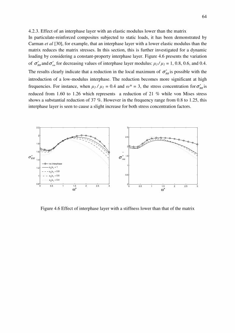
64
4.2.3. Effect of an interphase layer with an elastic modulus lower than the matrix
In particulate-reinforced composites subjected to static loads, it has been demonstrated by
Carman et al [30], for example, that an interphase layer with a lower elastic modulus than the
matrix reduces the matrix stresses. In this section, this is further investigated for a dynamic
loading by considering a constant-property interphase layer. Figure 4.6 presents the variation
of RR
σ ∗ andvm
σ ∗ for decreasing values of interphase layer modulus: µ3 / µ1 = 1, 0.8, 0.6, and 0.4.
The results clearly indicate that a reduction in the local maximum of RR
σ ∗ is possible with the
introduction of a low-modulus interphase. The reduction becomes more significant at high
frequencies. For instance, when µ3 / µ1 = 0.4 and ω* = 3, the stress concentration forRR
σ ∗ is
reduced from 1.60 to 1.26 which represents a reduction of 21 % while von Mises stress
shows a substantial reduction of 37 %. However in the frequency range from 0.8 to 1.25, this
interphase layer is seen to cause a slight increase for both stress concentration factors.
0 0.5 1 1.5 2 2.5 30.8
1
1.2
1.4
1.6
1.8
2
2.2
ω*
σ* rr
no interphase
µ3/µ
1 = 1
µ3/µ
1 = 0.8
µ3/µ
1 = 0.6
µ3/µ
1 = 0.4
0 0.5 1 1.5 2 2.5 30
0.5
1
1.5
2
2.5
3
ω*
σ* v
m
Figure 4.6 Effect of interphase layer with a stiffness lower than that of the matrix
RRσ ∗
∗vmσ

65
4.2.4. Effect of Poisson’s ratio
The values of the Poisson’s ratio of the interphase layer have thus far been kept constant. It
will be investigated now how this variable affects the stress concentration in the matrix.
Figure 4.7 represents the effect that the Poisson’s ratio of the interphase layer has on the
stress concentration for RR
σ ∗ andvm
σ ∗ when µ3 / µ1 = 0.4. It can be seen that there is a consistent
reduction of stress concentration forRR
σ ∗ when the Poisson’s ratio of the interphase layer is
decreased and this reduction is significant at high frequencies. In fact, a reduction of 41% can
be seen when the normalised frequency is 3. A similar trend is observed forvm
σ ∗
until the
normalised frequency becomes 2.4. At this frequency vm
σ ∗ exhibits a maximum reduction of
44%. However, vm
σ ∗ starts increasing slightly in the frequency range 2.4 to 3 when the
Poisson’s ratio of the interphase is 0.2 or 0.1. This change in behavior of vm
σ ∗
is due to the
shift in the angular position of the maximum from 180° to 90°. This is illustrated in Figure
4.8 which shows the angular location at which the maximum value for vm
σ ∗
occurs for various
frequencies.
0 0.5 1 1.5 2 2.5 30.8
1
1.2
1.4
1.6
1.8
2
2.2
ω*
σ* rr
no interphase
ν3 = 0.3
ν3 = 0.2
ν3 = 0.1
0 0.5 1 1.5 2 2.5 30
0.5
1
1.5
2
2.5
3
ω*
σ* v
m
Figure 4.7 Effect of Poisson’s ratio of the interphase on the stress concentration
RRσ ∗
∗vmσ

66
0 0.5 1 1.5 2 2.5 30
20
40
60
80
100
120
140
160
180
200
ω*
θ (
deg)
no interphase
ν1 = 0.3
ν1 = 0.2
ν1 = 0.1
Figure 4.8 Angular location of maximum von Mises stress for different Poisson’s ratios (µ3 /
µ1 = 0.4, ρ3 / ρ1 =1)
4.2.5. Effect of Density
Figure 4.9 shows the effect of density of the interphase layer for the case µ3 / µ1 = 0.4 and νi =
0.1. The density of the interphase, be it lower or higher than that of the matrix, seems to have
little influence for normalised frequencies up to 2.2. At frequencies higher than 2.2, an
interphase lighter than the matrix could cause a small reduction in stress concentration.
0 0.5 1 1.5 2 2.5 30
0.5
1
1.5
2
2.5
3
ω*
σ* v
m
no interphase
ρ3/ρ
1 = 2.2
ρ3/ρ
1 = 2
ρ3/ρ
1 = 1.77
ρ3/ρ
1 = 1.4
0 0.5 1 1.5 2 2.5 30
0.5
1
1.5
2
2.5
3
ω*
σ* v
m
no interphase
ρ3/ρ
1 = 1
ρ3/ρ
1 = 0.7
ρ3/ρ
1 = 0.5
Figure 4.9 Effect of density of interphase layer on maximum von Mises stress (µ3 / µ1 = 0.4,
ν3 = 0.1, ν2 = ν1 = 0.3)
∗vmσ
∗vmσ
67
4.3. Conclusion
The effect of an interphase layer on the stress field caused by a dynamic loading in a Mg-
matrix surrounding SiC-particle has been studied in this paper. It was found that the
introduction of an interphase layer with an elastic modulus larger than the matrix or a
functionally graded interphase layer cannot offer significant reduction of stress concentration.
However, an interphase layer with an elastic modulus lower than the matrix caused
substantial decrease in stress concentration at high frequencies. The amount of reduction
depends strongly on the frequency. A reduction of 21% for RRσ ∗ and 37% for ∗vmσ could be
achieved at the normalized frequency of 3 through the introduction of an interphase layer
whose modulus is 2.5 times lower than that of the matrix. The stress concentration could be
further reduced by decreasing the Poisson’s ratio of the interphase to 0.1. Here a maximum
reduction of 44% for von Mises stress concentration can be achieved at the normalised
frequency of 2.4.

68
5. Surface effects on the dynamic elastic state surrounding a
nanosized spherical particle
5.1. Problem Formulation
In the bulk of the solids the equilibrium and constitutive equations are the same as those in
the traditional elasticity theory Gurtin and Murdoch [37] and Gurtin et a.l [40]. Figure 5.1
shows geometry of a single spherical nano-particle of radius a embedded in an
infinitely large matrix with z-axis as the symmetry axis. Owing to the geometry the
problem is best described by spherical coordinates (R, φ, θ). The bulk material properties are
given by Lamé constants λi and µi and mass density by ρi. The subscripts i = 1 and 2 donate
matrix (medium 1) and nano-particle (medium 2). Spheroid is excited by time harmonic plane
SV (shear) waves propagating in the xz plane, parallel to the axis of symmetry. On
encountering the particle incident waves are reflected, refracted and scattered. The time
variation is assumed to be of the form e-iωt, where ω is the frequency of excitation.
Only time-harmonic excitation is considered. Since all field quantities have the same time
variation this term will be suppresses in all subsequent representations for notational
convenience.
Figure 5.1 Schematic illustration of the general problem.
R
Nano-Particle
Matrix
Incident wave

69
The nano-particle and matrix material is assumed to be homogeneous, linearly
elastic, isotropic and fully bonded. Assuming a harmonic steady-state loading and
from the theory of elasticity the displacement at any point within the bulk medium
must satisfy the equation (2.1) of motion:
In the matrix the wave field consists of both incident and scattered waves while the particle
consists of only refracted wave field. By denoting the incident and scattered waves by the
superscripts inc and sct respectively, the displacement vector U in the matrix has
contributions from both incident and scattered waves.
inc sct= +U U U (5.2)
While the incident wave field is known, the scattered wave field in the matrix and the
refracted field in the particle is unknown.
Before writing the displacement and stress expressions for incident, scattered and refracted
waves, the general expressions for displacement amplitudes of the equations (2.13) to (2.15)
and stress amplitudes of the equations (2.42) to (2.47) are rewritten in the following form:
1 1
1 21 2 22nR n n n nu a c P a c P= + (5.3)
1 1 1
1 23 2 24 3 25sin
n n n nn n n
dP dP Pu a c a c a c
d dθ
θ θ θ= + + (5.4)
1 1 1
1 23 2 24 3 25sin sin
n n n nn n n
P P dPu a c a c a c
dφ
θ θ θ= + + (5.5)
1 1
1 2 2 1nRR n n n na c P a c Pσ = + (5.6)
1 1 1
1 9 2 10 3 11sin
n n n nR n n n
dP dP Pa c a c a c
d dθσ
θ θ θ= + + (5.7)
1 1 1
1 9 2 10 3 11sin sin
n n n nR n n n
P P dPa c a c a c
dφσ
θ θ θ= + + (5.8)
2 1 2 11 1
1 3 4 2 5 62 2
11
3 12
1cot
sin
n n nn n n n
nn n
d P d Pa c P c a c P c
d d
dPa c P
d
θθσθ θ
θθ θ
= + + +
+ −
(5.9)
11 1
1 3 4 2
11 1
2 5 6 2
11
3 12
1cot
sin
1cot
sin
1cot
sin
n nn n n
nn n n
nn n
dPa c P c P
d
dPa c P c P
d
dPa c P
d
φφσ θθ θ
θθ θ
θθ θ
= + −
+ + −
+ −
(5.10)

70
( ) ( )
( ) ( )
( ) ( )
1 11 4 12
1 12 6 12
2 2 1 13 12 12
11 cos 1
sin
11 cos 1
sin
1 11 1 sin 1 cos
2sin
nn n n
n n n
n n n
a c n P n P
a c n P n P
a c n n n P n P
θφσ θθ
θθ
θ θθ
−
−
−
= − − +
+ − − +
+ − − − + +
(5.11)
where
( ) ( )2 2 21 12
2 12
2n nc n n R Z R RZ R
R
µβ α α α+
= − − +
(5.12)
( )( ) ( ) ( )2 12
121 n n
n nc n Z R RZ R
R
µβ β β
β+
+ = − − (5.13)
( ) ( )2 2 2 23 12
2 1
2n nc n R R Z R RZ R
R
µα β α α α+
= + − −
(5.14)
( )4 2
2nc Z R
R
µα= (5.15)
( ) ( )5 2
2 11 nc n n Z R
R
µβ
β= + (5.16)
( ) ( ) ( )6 12
2 11 n nc n Z R RZ R
R
µβ β β
β+ = + − (5.17)
( ) ( ) ( )9 12
21 n nc n Z R RZ R
R
µα α α+ = − − (5.18)
( ) ( )2 2 210 12
2 1 1
2n nc n n R Z R RZ R
R
µβ β β β
β+
= − − +
(5.19)
( ) ( ) ( )11 11 n nc n Z R RZ RR
µβ β β+ = − − (5.20)
( )12
2nc Z R
R
µβ= (5.21)
( ) ( )21 1n n
nc Z R Z R
Rα α α+= − (5.22)
( )( )
22 1nZ R
c n nR
β
β= +
(5.23)
( )23
nZ Rc
R
α= (5.24)
( )( )
( )24 11n
n
Z Rc n Z R
R
ββ
β+= + − (5.25)
( )25 nc Z Rβ= (5.26)
In the above and the equations that follow, the argument (cosθ) for 1
nP and its derivatives has
been suppressed for notational convenience.
The incident wave displacement and stresses are described in section 3.1.3.

71
The expressions for scattered wave displacements and stresses are given in section
3.1.4 equations (3.32) to (3.34) and (3.38) to (3.40). Since only three stress
components for scattered wave are given, all six can be obtained from equations
(5.3) to (5.11) by replacing the function Zn by ( )1
nh in the expressions for c1, c2,..., etc
with α and β being those of matrix.
5.1.1. Refracted waves in the particle
The refracted waves, being confined in the spherical particle, are standing waves. The
potentials χ, ψ and φ in the equation (2.2) are now given by:
( ) ( ) 11 2, , cosrfrn n nR b j R Pχ φ θ α φ=∑ (5.27)
( ) ( ) 12 2, , cosrfr
n n nR b j R Pψ φ θ β φ=∑ (5.28)
( ) ( ) 13 2, , sinrfr
n n nR b j R Pϕ φ θ β φ=∑ (5.29)
where superscript rfr refers to the refracted wave, b1n, b2n and b3n are as yet unknown
amplitude coefficients and subscript 2 refers to the particle medium,
By substituting equations (5.27) to (5.29) into equation (2.2) and the resulting expressions
into equations (2.13) to (2.15) and equations (2.30) to (2.35) the displacements and stresses in
spherical coordinate system due to refracted field in the particle are obtained. These
expressions are given in equations (5.3) to (5.11) by replacing the function Zn by jn in the
expressions for c1, c2,...,etc with α and β being those of a particle.
5.1.2. Surface/interface elasticity
In the surface/interface elasticity theory an interface is considered as a negligibly thin surface
or a membrane glued to the underlying bulk materials without slipping and its inertia can be
neglected for dynamic problems. The elastic constants of the membrane are different from
those of its adjoining materials and are given by constants µs and λs. This leads to a set of
nonclassical boundary conditions at the interface. Basic equations of the surface/interface
elasticity theory are reviewed here.
The relation between surface energy density ( )αβεΓ and the surface stress tensor s
αβσ is
0s
sαβ αβαβ
σ ι δε
∂Γ= +
∂ (5.30)
where superscript s denotes the surface, 0ι is the residual surface stress under unstrained
conditions, αβδ
is the Kronecker delta and s
αβε
the second rank tensor of the
surface/interface strain.
72
The equilibrium condition on the surface can be written as
, 0,s sij i jt n nα βα β αβ αβσ σ σ κ+ = = (5.31)
( ) ( )0 0 02s s sαβ αβ γγ αβ αγ γβσ ι δ λ ι ε δ µ ι δ ε= + + + − (5.32)
where superscript s denotes the surface, tα is the tangential component of the traction s
i ij jt nσ=
in the direction χα ,
ijσ is the change of the bulk stress tensor across the
surface/interface, s
αβσ is the stress tensor of the surface/interface, ni is the normal vector of
the surface/interface, αβκ is the surface/interface curvature.
For the isotropic surface/interface the stresses are given by:
2s s s s sαβ γγ αβ αβσ λ ε δ µ ε= + (5.33)
5.1.3. Continuity conditions
The surface/interface strains in spherical coordinates in terms of the matrix stresses in the
bulk are given by
( )1 1 1 11s
RRv vE
θθ θθ θθ φφε ε σ σ σ= = − − (5.34)
( )1 1 1 11s
RRv vE
φφ φφ φφ θθε ε σ σ σ= = − − (5.35)
1
2
s
G
θφ
θφ
σε = (5.36)
where superscript 1 refers to the matrix medium. E, G and v donate Young’s modulus, shear
modulus and Poisson’s ratio of the matrix respectively.
The stress-strain relationships for the surface/interface from equation (5.33) are given by:
( ) 2s s s s s s
θθ θθ φφ θθσ λ ε ε µ ε= + + (5.37)
( ) 2s s s s s s
φφ θθ φφ φφσ λ ε ε µ ε= + + (5.38)
2s s s
θφ θφσ µ ε= (5.39)

73
Substituting equations (5.40) to (5.42) into equations (5.37) to (5.39) and resulting
expressions into equilibrium condition of equation (5.33) the surface effects on the interface
of the nano-sized spherical particle of radius a and the matrix are obtained:
( ) ( )1 2 1 s sRR RR
aθθ φφσ σ σ σ− = + (5.40)
( ) ( )1 2 1 1 1 1cot
sin
sss s
R Ra a a
θφθθθ θ θθ φφ
δσδσσ σ σ σ θ
δθ θ δφ
− = − + − +
(5.41)
( )1 2 1 1 12cot
sin
s s
sR R
a a
θφ φφφ φ θφ
δσ δσσ σ θ σ
δθ θ δφ
− = − + +
(5.42)
where 1 inc sct
RR RR RRσ σ σ= + and same applies for 1
Rθσ and 1
Rφσ . Superscript 2 refer to the refracted
wave field in the particle.
The displacement continuity conditions on the interface require that:
1 2R Ru u= (5.43) 1 2u uθ θ= (5.44)
1 2u uφ φ= (5.45)
Where 1 inc sct
R R Ru u u= + and the same applies for 1
uθ and 1uφ .
Substituting equations (5.34) to (5.36) into (5.37) to (5.39) and the resulting expressions into
equations (5.40) to (5.42) the interface stress conditions in terms of bulk stresses are obtained
( ) ( ) ( ) ( )1 2 1 1 11 2 1 1 1 22 1 4RR RR RRk k v v k kθθ φφσ σ σ σ σ− = + − + − + (5.46)
( ) ( )
( ) ( )( )
( )
111 2
1 1 2 1 2
11 1
1 1 2 2
12 1
1 2 1 2
2 2 1
12 1
sin
R R
RR
v k k v k k
v k k k v
k v
φφθθθ θ
θθ φφ
θφ
δσδσσ σ
δθ δθ
δσσ σ
δθ
σθ
− = − + − − −
+ + − + +
+ +
(5.47)
( )
( ) ( ) ( ){ }
11 2 1
2 1
1 1 11 1 2 1 1 2 1 1 2
2 1 2 cot
11 2 1 2
sin
R R
RR
k v
v k k v k k v k k
θφφ φ θφ
θθ φφ
δσσ σ σ θ
δθ
σ σ σθ
− = + +
+ − − + − + − +
(5.48)
where k1 and k2 are dimensionless parameters

74
11
s
kE a
λ= , 2
1
s
kE a
µ= (5.49)
With a particle size approaching macroscopic values the terms µ2 and λ2, and consequently k1
and k2 approach zero. The surface/interface effects disappear in this case and the equations
(5.40) to (5.42) reduce to the solution of the classical elasticity. In view of the modelling
different material properties of the matrix and the inhomogeneity, as the ratio 2 1 0µ µ →
the
inhomogeneity becomes a cavity, however as 2 1µ µ → ∞ the inhomogeneity becomes a rigid
inclusion.
By invoking the orthogonality relations of Legendre polynomials in equations (5.43) to
(5.48), one obtains, for each n ≥ 1, two sets of simultaneous algebraic equations which can be
expressed in matrix form as:
[ ]{ } { }nE b f= (5.50)
[ ]{ } { }nP d q= (5.51)
where the vector{ }nb contains the unknown coefficients [a1n a2n b1n b2n]T and vector { }nd
contains the unknown coefficients [a3n b3n]T. The elements of [ ]E and [ ]P and vectors { }f
and { }q are given in the Appendix D. Equations (5.50) and (5.51) can be solved to determine
the coefficients a1n, a2n, a3n, b1n, b2n and b3n.
5.2. Numerical results and discussion
In the absence of the nano-particle, the stress field at any point in the medium can be
expressed in rectangular coordinates as
1
1 1i z i t
xz zx i eβ ωσ σ µ β −= = (5.52)
where subscript 1 refers to the matrix medium. With all other stress components being zero
the maximum value of the stresses is µ1β1.
In the presence of the nano-particle, the stress field is significantly different from that given
by equation (5.52) due to scattering. The nonzero stresses on the surface of the particle
are RRσ , Rφσ and Rθσ . The results have the general form
( ) ( ) i tR iI f e ωσ φ −= + (5.53)

75
where ƒ(φ) is either cosφ or sinφ, the real part R represents the solution at t = 0 and
T/2, and the imaginary part I represents the solution at t = T/4 and 3T/4, T being the
period of excitation. The absolute value (R2 + I
2)
1/2 is the maximum stress that occurs at
some instant depending on the phase-shift.
These stresses are expressed in dimensionless form by normalizing with respect to the
maximum value of the incident stress field, µ1β1:
1 1
, ,ij
ij i j tσ
σ φµ β
∗ = = (5.54)
Thus the values of ijσ ∗ can be considered as dynamic stress concentration factors. They
depend on the aspect ratio of the particle and the frequency of excitation; the latter is
expressed in non-dimensional form through
1
1
aρ
ω ωµ
∗ = (5.55)
where a, as defined earlier, is the radius of the nano-particle in the x-y plane.
The nature of the dynamic excitation is better appreciated by considering the limiting static
case. When the frequency approaches zero, the applied stress field at infinity approaches
0xz zxσ σ σ= = (5.56)
xx yy zz xy yzσ σ σ σ σ= = = = (5.57)
where 0σ is a constant. The stress field of equations (5.56) and (5.57) is pure shear. Thus, the
results presented herein are for the dynamic counterpart of this shear load.
In the following examples the effects of parameter k2 and normalized frequency ∗ω on the
stress concentration values in the matrix at the interface has been examined. Parameter
k1=0 and ν1= ν2=0.3. In many practical applications of particulate-reinforced composites a
common observation is that failure often initiates in the matrix at the interface between the
particle and matrix which. This confirms the high stress concentration values obtained in this
study for different stress components. Particles often have considerably larger modulus and
substantially higher yield stress values than the matrix and initiation of failure will therefore
most likely take place within the matrix. For this reason, we will henceforth limit our
attention to the state of stress in the matrix at the interface only.
Figures 5.1 to 5.2 illustrate the angular distribution of RRσ ∗ and Rφσ∗
for six k2 values and
normalized frequencies of ∗ω = 0.1 and 3. The other stress values are not shown since their
values consistently fall between those of RRσ ∗
and Rφσ∗ . It can be seen that both

76
nondimensional frequency and k2 have significant influence on stress distribution. At a
very small normalized frequency of 0.1 the wavelength of the incident wave is much
larger than the nano-particle radius and hardly any dynamic effect is expected. The
dynamic solution can be regarded as quasi-static and dynamic load is given approximately
by equations (5.56) and (5.57) which exhibit symmetry with respect to the z = 0 plane.
As seen in figures 5.1 to 5.2 the resulting stress field is also symmetric about this plane
for all k2 values. The maximum values of RRσ ∗ occur at θ π = 0.25, 0.75 and that of Rφσ∗
occur θ π = 0 and 1. The influence of k2 on RRσ ∗ and Rφσ∗
stress concentration values is the
highest at these same values of θ π . The most significant reduction of RRσ ∗
stress
concentration values occur at k2 values greater than 1. For values lower than 1 the stress
concentration reduction is not significant. The effect of k2 values on Rφσ∗ stress
concentration values is less than for RRσ ∗ . With increasing k2 values in the range below 1
show more or less the same stress concentration reduction as values above 1, which is
different to that of RRσ ∗ .
For the normalized frequency of 3.0 the wavelength is about the same size as the
diameter of the particle and a great deal of scattering occurs (figures 5.2) which results in
a stress distribution being quite different from the quasi-static solution. The dynamic stress
concentration distribution is no longer symmetric about the θ π = 0.5. The influence of k2
values on both RRσ ∗
and Rφσ∗
occur at the peak stress concentration values. The effect of k2
values on RRσ ∗ occur across greater angle range at higher normalized frequency than is the
case at quasi-static loading. The increasing k2 values result in higher Rφσ∗
stress
concentration values at θ π range below 0.65.
The radial distribution of RRσ ∗ , Rφσ∗ and Rθσ ∗ in the matrix at θ π = 0.75 is illustrated in
figures 5.3 and 5.4 for ω*= 0.1 and 2. The stress concentration of Rθσ ∗
in figure 5.3 is not
shown as its values fall far below that of Rφσ∗ . As the radius increase all three stress
components converge to incident field values as expected. The maximum values of the
stresses occur at or near the interface indicating the most likely location of the matrix
failure. The stress concentration values are mostly affected by nano-sized particle
properties at or very near the interface. This effect then relatively quickly disappears as
distance from the particle increases, as expected.
The influence of the k2 parameter and the normalized frequency on the peak stress
concentration values for RRσ ∗ and Rφσ∗ is shown in figure 5.5. The increasing k2 values shows a
reduction of RRσ ∗
peak stress concentration values throughout the frequency range. A
significant decrease occurs for k2 values greater than 1, which is reflected in figures 5.1
and 5.2. The peak stress concentration values of Rφσ∗ experience a drop for k2 values lower
than 1 throughout the frequency range. However the values show an increase for k2 values
greater than 1 at ∗ω > 0.7.

77
Figures 5.6 and 5.7 show the effect of stiffness ratio µ* of nano-particle to matrix on the
peak stress concentration values of RRσ ∗
and Rφσ∗ that occur over a range of normalized
frequencies 0 < ω* < 3. Values of figure 3.6 and 3.7 are computed for k2 value of 0.5 and
2 respectively. It is evident that the higher particle stiffness value result in a steady
increase in peak stress concentration values of RRσ ∗
throughout the considered normalized
frequency range and for both k2 values. This increase in stress concentration values
becomes progressively higher with the increase in frequency. The values of Rφσ∗
however
exhibit initially a reduction in stress concentration values throughout the frequency range
considered as the particle-matrix stiffness ratio increases from a very low ratio. As the
particle-matrix stiffness ratio increases further the effect is reversed showing quite a large
increase in stress concentration values. The greatest effect is shown at very low
frequencies.
Figure 5.1 Angular distribution of stress concentration in the matrix at the nano-particle
matrix interface for ω*= 0.1 (ρ*=1, µ*=8, ν1= ν2=0.3)

78
Figure 5.2 Angular distribution of stress concentration in the matrix at the nano-particle
matrix interface for ω*= 3 (ρ*=1, µ*=8, ν1= ν2=0.3)

79
Figure 5.3 Radial distribution of stress concentration in the matrix at θ π = 0.75 angle for
ω*= 0.1 (ρ*=1, µ*=8, ν1= ν2=0.3)
Figure 5.4 Radial distribution of stress concentration in the matrix at θ π = 0.75 angle for
ω*= 2 (ρ*=1, µ*=8, ν1= ν2=0.3)

80
Figure 5.5 Effect of k2 on the peak stress concentration values in the matrix at the nano-
particle matrix interface (ρ*=1, µ*=8, ν1= ν2=0.3)
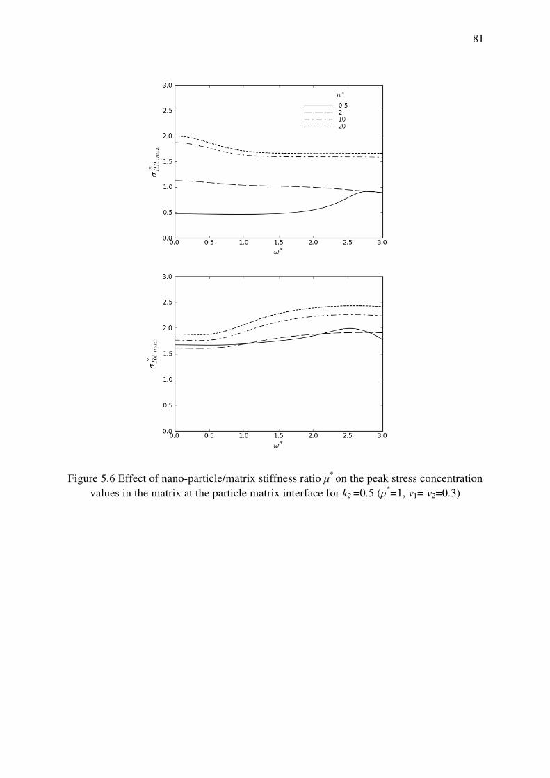
81
Figure 5.6 Effect of nano-particle/matrix stiffness ratio µ* on the peak stress concentration
values in the matrix at the particle matrix interface for k2 =0.5 (ρ*=1, ν1= ν2=0.3)

82
Figure 5.7 Effect of nano-particle/matrix stiffness ratio µ* on the peak stress concentration
values in the matrix at the particle matrix interface for k2 =2 (ρ*=1, ν1= ν2=0.3)
5.3. Conclusion
The study presents the effect of surface/interface elasticity on the dynamic stress field at the
interface of the nanosized particle and the matrix due to a shear wave loading. It has been
shown that the dynamic stress field at the particle-matrix interface is significantly affected by
surface/interface elasticity as the particle size reduces to nanometers. The surface/interface
effect is localized to a region at or very near the interface and quickly disappears away from
interface. The increasing surface elastic constant µs can significantly reduce the stress
concentration values concentration values at the nano-particle matrix interface.

83
6. Summary and final conclusion
The study deals with determining stress concentration in a particle reinforced composite at
the particle-matrix interface as a result of interaction with elastic waves. Stress concentration
at the interphase has been directly linked to formation of microcracks that eventually lead to
failure. The investigation here analysed three interrelated problems by expanding techniques
previously developed. All the analysis assumed low concentration of particles and therefore
interaction of neighboring particles was ignored. All the materials are assumed linear elastic
and perfectly bonded to each other. The investigation considered the effects of prolate
spheroidal shape of a particle, nanoparticle surface/interface energy and particle-matrix
interphase layers on dynamic stress concentration.
Since the analysis of the dynamic stress concentration around a particle due to dynamic
waves is limited to a simple spherical shape, a hybrid technique was used. The technique is
an extension of the already developed hybrid technique for axisymmetric loading to
incorporate three dimensionality of asymmetric shear loading. It uses the finite element
method with spherical wave functions. The analysis showed that the higher aspect ratios of
the spheroidal particle result in increase in dynamic stress concentration. The increase
however depends on both frequency of incident wave and aspect ratio. At higher wave
frequencies, high values of spheroidal particle stiffness can result in 147% increase in
peak stress concentration from the quasi-static values.
As the interphase layer in MMCs either occurs naturally or is intentionally introduced it is
important to consider its effect on dynamic stress concentration. It is desirable to also
investigate the properties of the interphase layer to potentially reduce the dynamic stress
concentration at the particle-matrix interface. The study considered interphase effect in a
Mg-matrix surrounding a SiC-particle. Both functionally graded and constant property
interphase layers were considered. The analysis showed that the functionally graded
interphase layer does not offer any significant stress concentration reduction. However a
constant property interphase layer with elastic modulus and Poisson’s ratio lower than the
matrix can significantly reduce the stress concentration.
Stress states of the materials at nanoscale are found to differ from those at macroscale. This
variation of the material behavior around the free surface or interface, as structures reduce to
nano-meters has mainly contributed to Surface/interface energy. Previous two studies
outlined in the paragraphs above have been extended here to include free surface/interface
effects as the particle size reduces to nanometers. The nano-particle was subject to shear
dynamic waves and by considering the effects of surface/interface elasticity, stress
concentration values at the interface with matrix were obtained. The results showed that
Surface/interface elasticity of the nanosized particle has a significant effect on dynamic stress
field at the particle-matrix interface. The increasing surface elastic constant µs greatly reduces
the stress concentration values at the nano-particle matrix interface. This effect is however
localized near the interface and quickly disappears away from interface.

84
The findings show that the particle shape, particle size, interphase layer properties as well as
particle and matrix properties all have a significant influence on dynamic stress concentration
at the particle-matrix interface.

85
References
[1] www.globalspec.com/reference/69955/203279/chapter-15-composite-materials.
Figure 15.1: Different types of reinforcement for composites.
[2] www.tms.org/pubs/journals/JOM/0104/Rawal-0104.html. Figure 1. Photo courtesy of
U.S. Air Force/NASA.
[3] www.cmt-ltd.com/html/mat_1.htm. Metal matrix composites, Figure Title: Properties
of AMCs versus conventional alloys.
[4] ASM Handbook, Vol 21 Composites, 2001.
[5] Davidson DL. The effect of particulate SiC on fatigue crack growth in a cast-extruded
aluminium alloy composite. Metalurgicall and Materials Transactions, 1991, vol. 22,
pp. 97-209.
[6] Sternberg E. Three-dimensional stress concentrations in the theory of elasticity.
Applied Mechanics Rev, 1958, vol. 11, pp. 1-5.
[7] Neuber H, Hahn HG. Stress concentration in scientific research and engineering.
Applied Mechanics Rev, 1966, vol. 19, pp. 187-286.
[8] Tan SC. Stress concentrations laminated composites. Lancaster, PA: Technomic
Publishing Co., 1994.
[9] Prokic, A, Lukic, D, Anagnosti, P. Stress – strain field around elliptic cavities in
elastic continuum. European Journal of Mechanics, 2009, 28, 86-93.
[10] Wang Z, Chen TK, Lloyd DJ. Stress distribution in particulate reinforced metal
matrix composites subjected to external load. Metalurgicall and Materials
Transactions, 1993, vol. 24A, pp. 197-207.
[11] Agarwal BD, Broutman LJ. Three-dimensional finite element analysis of spherical
particle composites. Fiber Science and Technology, 1974, vol. 7, pp. 63-72.
[12] Kassam ZHA, Zhang RJ, Wang Z. Finite element simulation to investigate interaction
between crack and particulate reinforcements in metal-matrix composites. Materials
Science and Engineering, 1995, vol. A203, pp. 286-299.
[13] Pao YH, Mow CC. Diffraction of elastic waves and dynamic stress concentrations.
New York: Crane and Russak, 1973.
[14] Bogan SD, Hinders MK. Dynamic stress concentrations in fiber-reinforced
composites with interface layers. Journal of Composite Materials, 1993, vol. 27, pp.
1272-1312.
[15] Ying CF, Truell R. Scattering of a plane longitudinal wave by a spherical obstacle in
an isotropically elastic solid. Journal of Applied Physics, 1956, vol. 27, pp. 1086-
1184.
[16] Bostrom A. Scattering by a smooth elastic obstacle. Journal of Acoustic Society of
America, 1980, vol. 67, pp. 1904-1917.
[17] Shindo Y, Nozaki H, Datta SK. Effect of interface layers on elastic wave propagation
in a metal matrix composite reinforced by particles. Journal of Applied Mechanics,
1995; 62; 178-85.

86
[18] Paskaramoorthy R, Meguid SA. Large internal stresses in particle-reinforced
composites subjected to dynamic loads. Journal of Composite Science and
Technology, 1999; vol. 59: pp. 1361-67.
[19] Paskaramoorthy R, Kienhöfer F, Chandler HD. The response of particle-reinforced
composites to asymmetric dynamic loading. Journal of Composite Science and
Technology, 2002, vol. 62, pp. 223-232.
[20] Datta, SK. Diffraction of plane elastic waves by ellipsoidal inclusions. Journal of
Acoustic Society of America, 1997, 61, 1432-1537.
[21] Willis, JR. A polarization approach to the scattering of elastic waves – I. Scattering by
a single inclusion. Journal of Mechanics and Physics of Solids, 1980, 28, 287-305.
[22] Paskaramoorthy R, Datta SK, Shah AH. Effect of interface layers on scattering of
elastic waves. Journal of Applied Mechanics, 1988; 55: 871-8.
[23] Olsson, P, Datta, SK., and Bostrom, A. Elastodynamic scattering from inclusions
surrounded by thin interface layers. Journal of Applied Mechanics, 1990, 57, 672-676.
[24] Meguid, SA, Wang, XD. Wave scattering from partially-debonded inhomogeneities in
advanced ceramics. Presented at the 1997. Joint ASME, ASCE and SES Summer
Meeting, 29 June-2 July, Northwestern University.
[25] R. Paskaramoorthy, F. Kienhöfer, and S. A. Meguid . “The Dynamic Stress Field in
the Matrix Surrounding a Spheroidal Particle”. Journal of Composite Materials, Aug
2002; vol. 36: pp. 1803 - 1824.
[26] Madhukar MS, Drzal LT. Fiber-matrix adhesion and its effects on composite
mechanical properties: I. Inplane and interlaminar shear behavior of graphite/epoxy
composites. Journal of Composite Materials, 1991, vol. 25, pp. 932-958.
[27] Wu Y, Dong Z. Three dimensional finite element analysis of composites with coated
spherical inclusions. Materials Science and Engineering, 1995, vol. 203, pp. 314-337.
[28] Ghosn LJ, Lerch BA. Optimum interface properties for metal matrix composites.
NASA Technical Memorandum, 1989, vol. 102295, pp. 1-19.
[29] Jansson S, Leckie FA. Reduction of thermal stresses in continuous fibre reinforced
metal matrix composites with interface layers. Journal of Composite Materials, 1992,
vol. 26, pp. 1474-1486.
[30] Carman GP, Averill RC, Reifsnider KL, Reddy JN. Optimization of fiber coatings to
minimize stress concentrations in composite materials. Journal of Composite
Materials, 1993, vol. 27, pp. 589-612.
[31] Al-Ostaz A, Jasiuk I. Effect of interface and random arrangement of inclusions on
the local stresses in composite materials. Durability of Composite Materials, 1994;
51: 207-217.
[32] Foldy LL. Multiple scattering theory of waves. Physical Review, 1945; 67: 107-119.
[33] Lee CS, Ahn AH, DeJonghe LC, Thomas G. Effect of functionally graded material
(FGM) layers on the residual stress of polytypoidally joined Si3N4–Al2O3, Materials
Science and Engineering: A, 2006, vol. 434, pp. 160-165.
[34] Cammarata, RC. Surface and interface stresses effects in thin films. Progress in
Surface Science, 1994, 46, 1–38.
[35] Cammarata, RC. Surface and interface stress effects on interfacial and nanostructured
materials. Materials Science and Engineering: A, 1997,237, 180–184.

87
[36] Streitz, FH, Cammarata, RC, and Sieradzki, K. Surface-stress effects on elastic
properties. I. Thin metal films. Physics Rev., B, 1994, 49, 10699–10706.
[37] Gurtin, ME, and Murdoch, AI. Acontinuum theory of elastic material surfaces.
Archives of Rational Mechanics and Analysis, 1975, 57, 291–323.
[38] Gurtin, ME, and Murdoch, AI. Surface stress in solids. International Journal of Solids
and Structures, 1978, 14, 431–440.
[39] Murdoch, AI. Thermodynamical theory of elastic-material interfaces. Quarterly
Journal of Mechanics and Applied Mathematics, 1976, 29, 245–275.
[40] Gurtin, M E, Weissmüller, J, and Larché, F. Ageneral theory of curved deformable
interfaces in solids at equilibrium. Philosophical. Magazine, A, 1998,78, 1093–1109.
[41] Shenoy, VB. Atomistic calculations of elastic properties of metallic fcc crystal
surfaces. Physics Rev., B, 2005, 71, 094104-1–11.
[42] Miller, RE, and Shenoy, VB. Size-dependent elastic properties of nanosized structural
elements. Nanotechnology, 2000, 11, 139–147.
[43] Shenoy, VB. Size-dependent rigidities of nanosized torsional elements. International
Journal of Solids and Structures, 2002, 39, 4039–4052.
[44] Cuenot, S, Fr’etigny, C, Demoustier-Champagne, S, and Nysten, B. Surface tension
effect on the mechanical properties of nanomaterials measured by atomic force
microscopy. Physics Rev., B, 2004, 69, 165410–165413.
[45] Jing, GY, Duan, HL, Sun, XM, Zhang, ZS, Xu, J, Li, YD, Wang, J, and Yu, DP.
Surface effects on elastic properties of silver nanowires: contact atomic-force
microscopy. Physics Rev., B 2006, 73, 235409-1–6.
[46] Sharma, P, Ganti, S, and Bhate, N. Effect of surfaces on the sizedependent elastic
state of nano-inhomogeneities. Applied Physics Letters, 2003, 82, 535–537.
[47] Fang, QH, and Liu, YW. Size-dependent interaction between an edge dislocation and
a nanoscale inhomogeneity with interface effects. Acta Materialia, 2006, 54, 4213–
4220.
[48] Wang, GF, and Wang, TJ. Deformation around a nanosized elliptical hole with
surface effect. Applied Physics Letters, 2006, 89, 161901-1–3.
[49] Paskaramoorthy, R., Meguid, SA. On the dynamic behavior of porous materials.
Journal of Solids and Structures, 2000, 37, 2341-2358.
[50] Wang, GF, Wang, TJ, and Feng, XQ. Surface effects on the diffraction of plane
compressional waves by a nanosized circular hole. Applied Physics Letters, 2006, 89,
231923-1–3.
[51] Wang, GF. Diffraction of shear waves by a nanosized spherical cavity. Journal of
Applied Physics, 2008,103, 053519-5.
[52] Wang, GF, Feng XQ, and Yu SW. Interface effects on the diffraction of plane
compressional waves by a nanosized spherical inclusion. Journal of Applied Physics,
2007,102, 043533.
[53] Cook, RD, Malkus, DS, Plesha, ME. Concepts and applications of finite element
analysis, third ed., John Wiley & Sons, New York, 1989.
[54] Lancaster, P. 1969. Theory of Matrices, pp. 301–307, Academic Press, New York.

88
[55] Dong, SB, 1981. Global-local finite element methods. In: Pilkey, W.D., Noor, A.K.
(Eds), State-of-the-Art Survey of Finite Element Methods (Chap. 14) ASME
Publication.
[56] Taya M. and Arsenault RJ. Metal Matrix Composites. Permagon Pres, New York,
1989.
[57] Gaofeng Q, Yujiu S, and Mingjing T. Mechanical Properties and Evaluation of
Magnesium Matrix Composites. Proceding of the Second International Conference of
Composite Science and Technology, Jun 1998, pp. 175-179.
[58] Ranganath S.A. Review on Particulate-reinforced Titanium Matrix Composites.
Journal of Material Science, vol. 32, 1997, pp. 1-16.
[59] Noor A.K. and Levine S.R. Composite Materials, vol 3: Flight-Vehicle Material,
Structures and Dynamic Assessment & Future Directions. Academic Press, 1974.
[60] Eshelby JD. 1957. The determination of the elastic field of an ellipsoidal inclusion
and related problems. Proceedings of Royal Society of London Series, A, 241:376–86.
[61] Eshelby JD. 1959. The elastic field outside an ellipsoidal inclusion. Proceedings of
Royal Society of London Series, A, 252:561–9.
[62] Koizumi M. 1997. FGM activities in Japan. Composites Part B; 28:1–4.
[63] Lee CS, Ahn AH, DeJonghe LC, Thomas G. 2006. Effect of functionally graded
material (FGM) layers on the residual stress of polytypoidally joined. Materials
Science and Engineering, A; 434:160–5.

89
Appendix A
Assuming { }sct
Bsph
q is known, equation (3.41) may be solved for { }a by minimizing the least
square error of the error function { }ε defined by
{ } [ ]{ } { }sB
sphG a qε = − (A.1)
The square of the 2ε , which is a scalar, is given by
{ } { }2T
ε ε ε∗= (A.2)
Substitution of (A1) in (A2) leads to
{ } [ ]{ } { } [ ]{ } { } { } { } { }2T TT TT T
s s s sB B B B
sph sphsph sph
a G G a q G a a G q q qε∗ ∗∗ ∗ ∗ ∗ = − − + (A.3)
Minimizing the square of the error with respect to{ }a yields
[ ]{ } { }T T
sB
sphG G a G q
∗ ∗ = (A.4)
Since
T
G∗ [ ]G is a square matrix, the Equation. (A4) can be solved for{ }a as
{ } [ ]{ }sB
spha H q= (A.5)
where
[ ] [ ]1
T T
H G G G
−∗ ∗ =
(A.6)
For Bp N≤ , [ ]H is the generalized inverse of [ ]G and the uniqueness of the operation is
assured (Lancaster [54]).

90
Appendix B
( ) ( ) ( )2 2 211 1 1 1 12
2 11,1 2
2n n
E n n R h R Rh RR
µβ α α α+
= − − +
(B.1)
( ) ( ) ( ) ( )11 1 1 12
1
2 ( 1)1,2 1 n n
n nE n h R R h R
R
µβ β β
β+
+= − − (B.2)
( ) ( ) ( )2 2 233 3 3 1 32
2 11,3 2
2n n
E n n R j R R j RR
µβ α α α+
= − − − +
(B.3)
( ) ( ) ( ) ( )33 3 1 32
3
2 ( 1)1, 4 1 n n
n nE n j R R j R
R
µβ β β
β+
+= − − − (B.4)
( ) ( ) ( )2 2 233 3 3 1 32
2 11,5 2
2n n
E n n R y R R y RR
µβ α α α+
= − − − +
(B.5)
( ) ( ) ( ) ( )33 3 1 32
3
2 ( 1)1,6 1 n n
n nE n y R R y R
R
µβ β β
β+
+= − − − (B.6)
( ) 07,1 =E (B.7)
( ) 08,1 =E (B.8)
( ) ( ) ( ) ( )11 1 1 12
22,1 1 n nE n h R R h R
R
µα α α+= − − (B.9)
( ) ( ) ( )2 2 211 1 1 1 12
1
2 1 12,2 2
2n n
E n n R h R R h RR
µβ β β β
β+
= − − +
(B.10)
( ) ( ) ( ) ( )33 3 1 32
22,3 1 n nE n j R R j R
R
µα α α+= − − − (B.11)
( ) ( ) ( )2 2 233 3 3 1 32
3
2 1 12,4
2n n
E n n R j R R j RR
µβ β β β
β+
= − − − +
(B.12)
( ) ( ) ( ) ( )33 3 1 32
22,5 1 n nE n y R R y R
R
µα α α+= − − − (B.13)
( ) ( ) ( )2 2 233 3 3 1 32
3
2 1 12,6
2n n
E n n R y R R y RR
µβ β β β
β+
= − − − +
(B.14)
( ) 0 7,2 =E (B.15)

91
( ) 0 8,2 =E (B.16)
( ) ( ) ( )1 1 1 13,1 n n
nE h R h R
Rα α α+
= −
(B.17)
( ) ( )( )1
1
3,2 1 nh R
E n nR
β
β= + (B.18)
( ) ( ) ( )3 3 1 33,3 n n
nE j R j R
rα α α+
= − −
(B.19)
( ) ( )( )3
3
3, 4 1 nj R
E n nR
β
β= − + (B.20)
( ) ( ) ( )3 3 1 33,5 n n
nE y R y R
Rα α α+
= − −
(B.21)
( ) ( )( )3
3
3,6 1 ny R
E n nR
β
β= − + (B.22)
( ) 07,3 =E (B.23)
( ) 08,3 =E (B.24)
( )( )14,1 n
h RE
R
α= (B.25)
( ) ( )( )
( )1
1 1
1
4, 2 1 n
n
h RE n h R
R
ββ
β+
= + −
(B.26)
( )( )34,3 n
j RE
R
α= − (B.27)
( ) ( )( )
( )3
1 3
3
4, 4 1 n
n
j RE n j R
R
ββ
β+
= − + −
(B.28)
( )( )34,5 n
y RE
R
α= − (B.29)
( ) ( )( )
( )3
1 3
3
4,6 1 n
n
y RE n y R
R
ββ
β+
= − + −
(B.30)

92
( ) 07,4 =E (B.31)
( ) 08,4 =E (B.32)
( ) 01,5 =E (B.33)
( ) 02,5 =E (B.34)
( ) ( ) ( )2 2 233 3 3 1 32
2 15,3 2
2n n
E n n R j R R j RR
µβ α α α+
= − − +
(B.35)
( ) ( ) ( ) ( )33 3 1 32
3
2 ( 1)5,4 1 n n
n nE n j R R j R
R
µβ β β
β+
+= − − (B.36)
( ) ( ) ( )2 2 233 3 3 1 32
2 15,5 2
2n n
E n n R y R R y RR
µβ α α α+
= − − +
(B.37)
( ) ( ) ( ) ( )33 3 1 32
3
2 ( 1)5,6 1 n n
n nE n y R R y R
R
µβ β β
β+
+= − − (B.38)
( ) ( ) ( )2 2 232 2 2 1 22
2 15,7 2
2n n
E n n R j R R j RR
µβ α α α+
= − − − +
(B.39)
( ) ( ) ( ) ( )22 2 1 22
2
2 ( 1)5,8 1 n n
n nE n j R R j R
R
µβ β β
β+
+= − − − (B.40)
( ) 01,6 =E (B.41)
( ) 02,6 =E (B.42)
( ) ( ) ( ) ( )33 3 1 32
26,3 1 n nE n j R R j R
R
µα α α+= − − (B.43)
( ) ( ) ( )2 2 233 3 3 1 32
3
2 1 16,4
2n n
E n n R j R R j RR
µβ β β β
β+
= − − +
(B.44)
( ) ( ) ( ) ( )33 3 1 32
26,5 1 n nE n y R R y R
R
µα α α+= − − (B.45)
( ) ( ) ( )2 2 233 3 3 1 32
3
2 1 16,6
2n n
E n n R y R R y RR
µβ β β β
β+
= − − +
(B.46)
( ) ( ) ( ) ( )2
2 2 1 22
26,7 1 n nE n j R R j R
R
µα α α+= − − − (B.47)

93
( ) ( ) ( )2 2 222 2 2 1 22
2
2 1 16,8
2n n
E n n R j R R j RR
µβ β β β
β+
= − − − +
(B.48)
( ) 01,7 =E (B.49)
( ) 02,7 =E (B.50)
( ) ( ) ( )3 3 1 37,3 n n
nE j R j R
Rα α α+
= −
(B.51)
( ) ( )( )3
3
7,4 1 nj R
E n nR
β
β= + (B.52)
( ) ( ) ( )3 3 1 37,5 n n
nE y R y R
Rα α α+
= −
(B.53)
( ) ( )( )3
3
7,6 1 ny R
E n nR
β
β= + (B.54)
( ) ( ) ( )2 2 1 27,7 n n
nE j R j R
Rα α α+
= − −
(B.55)
( ) ( )( )2
2
7,8 1 nj R
E n nR
β
β= − + (B.56)
( ) 01,8 =E (B.57)
( ) 02,8 =E (B.58)
( )( )38,3 n
j RE
R
α= (B.59)
( ) ( )( )
( )3
1 3
3
8, 4 1 n
n
j RE n j R
R
ββ
β+
= + −
(B.60)
( )( )38,5 n
y RE
R
α= (B.61)
( ) ( )( )
( )3
1 3
3
8,6 1 n
n
y RE n y R
R
ββ
β+
= + −
(B.62)
( )( )28,7 n
j RE
R
α= − (B.63)
( ) ( )( )
( )2
1 2
2
8,8 1 n
n
j RE n j R
R
ββ
β+
= − + −
(B.64)

94
( ) ( ) ( ) ( )2 2 211 1 1 1 12
2 11,1 2n 1 2
2
n
n nf i n n R j R R j R
R
µβ α α α+
= − + − − +
(B.65)
( ) ( ) ( ) ( ) ( )11 1 1 12
22,1 2n 1 1n
n nf i n j R R j RR
µα α α+
= − + − −
(B.66)
( ) ( ) ( ) ( )1 1 1 13,1 2n 1n
n n
nf i j R j R
Rα α α+
= − + −
(B.67)
( ) ( )( )1
1
4,1 2n 1 nnj R
f iR
α
β
= − +
(B.68)
( ) ( ) 01,81,5 =ftof (B.69)

95
Appendix C
Figure C.1. Finite element mesh for the spheroidal particle (b/a=3) for static loading case
Figure C.2. Finite element mesh for the spheroidal particle (b/a=5) for static loading case

96
Appendix D
The elements of the matrices [E] and [P] and vectors {f} and {q} in equations (4.50) and
(4.51) are given by:
( )11 1 3 3 3 42 1E c k c n n k c= − + + (D.1)
( )12 2 3 5 3 62 1E c k c n n k c= − + + (D.2)
13 10 1E k e= − (D.3)
14 10 2E k e= − (D.4)
( ) ( ) ( )21 9 6 1 4 5 3 4 4 4 5 41E c k c k k c n n k c k k c= + + + − + + −
(D.6)
( ) ( ) ( )22 10 6 2 4 5 5 4 6 4 5 61E c k c k k c n n k c k k c= + + + − + + −
(D.7)
23 9E e= − (D.8)
24 10E e= − (D.9)
31 21E c= (D.10)
32 22E c= (D.11)
33 21E e= − (D.12)
34 22E e= − (D.13)
41 23E c= (D.14)
42 24E c= (D.15)
43 23E e= − (D.16)
44 24E e= − (D.17)
( ) ( )( )
( )1
1 2 3 5 3 6
2 12 1
1
ni n
f d k d n n k dn n
++
= − − + + + (D.18)
( ) ( )( )
( ) ( ) ( )1
2 10 6 2 4 5 5 4 6 4 5 6
2 11
1
ni n
f d k d k k d n n k d k k dn n
++
= − + + + − + + − + (D.19)
( ) ( )( )
1
3 22
2 1
1
ni n
f dn n
++
= −+
(D.20)
( ) ( )( )
1
4 24
2 1
1
ni n
f dn n
++
= −+
(D.21)
( ) ( )11 11 4 5 12
11 1
2P c k k n n c
= + − − + +
(D.22)
12 11P e= − (D.23)
21 25P c= (D.24)
22 25P e= − (D.25)
( ) ( )( )
( ) ( )1 11 4 5 12
2 1 11 1
1 2
ni n
q d k k n n dn n
− + = + − − + + +
(D.26)
( ) ( )( )2 25
2 1
1
ni n
q dn n
− +=
+ (D.27)

97
where
( )( )( )
1 23
1 2
2 1
1 4
k k vk
v k k
+ −=
+ + (D.28)
( )4 1 21 2k k v k= − + (D.29)
( )5 1 21 2k k v k v= − + (D.30)
( )6 1 22k k k v= + (D.31)
( )101 2
1
1 4k
v k k=
+ + (D.32)
In the above equations c1, c2,..., etc are calculated using hn(1) for Zn and α and β are those
of matrix.
The d1, d2,..., etc have identical expressions as c1, c2,..., etc but are calculated using jn for
Zn and α and β are those of matrix.
The e1, e2,..., etc have identical expressions as c1, c2,..., etc but are calculated using jn for
Zn and α and β are those of the nano-particle.