Originally published as:

Jousset, P., Reinsch, T., Ryberg, T., Blanck, H., Clarke, A., Aghayev, R., Hersir, G. P., Henninges, J., Weber, M., Krawczyk, C. (2018): Dynamic strain determination using fibre-optic cables allows imaging of seismological and structural features. - Nature Communications, 9.

DOI: http://doi.org/10.1038/s41467-018-04860-y

ARTICLE

Dynamic strain determination using fibre-opticcables allows imaging of seismological andstructural featuresPhilippe Jousset 1, Thomas Reinsch 1, Trond Ryberg1, Hanna Blanck2, Andy Clarke3

Rufat Aghayev3, Gylfi P. Hersir2, Jan Henninges1, Michael Weber 1,4 & Charlotte M. Krawczyk 1,5

Natural hazard prediction and efficient crust exploration require dense seismic observations

both in time and space. Seismological techniques provide ground-motion data, whose

accuracy depends on sensor characteristics and spatial distribution. Here we demonstrate

that dynamic strain determination is possible with conventional fibre-optic cables deployed

for telecommunication. Extending recently distributed acoustic sensing (DAS) studies, we

present high resolution spatially un-aliased broadband strain data. We recorded seismic

signals from natural and man-made sources with 4-m spacing along a 15-km-long fibre-optic

cable layout on Reykjanes Peninsula, SW-Iceland. We identify with unprecedented resolution

structural features such as normal faults and volcanic dykes in the Reykjanes Oblique Rift,

allowing us to infer new dynamic fault processes. Conventional seismometer recordings,

acquired simultaneously, validate the spectral amplitude DAS response between 0.1 and

100 Hz bandwidth. We suggest that the networks of fibre-optic telecommunication lines

worldwide could be used as seismometers opening a new window for Earth hazard assess-

ment and exploration.

DOI: 10.1038/s41467-018-04860-y OPEN

1 GFZ German Research Centre for Geosciences, Telegrafenberg, Potsdam 14473, Germany. 2 ÍSOR Iceland GeoSurvey, Grensásvegi 9, Reykjavik 108, Iceland.3 Silixa Ltd., Silixa House, 230 Centennial Park, Centennial Avenue, Elstree WD6 3SN, UK. 4 Institute of Earth and Environmental Science, University ofPotsdam, Potsdam 14476, Germany. 5 Institute for Applied Geosciences, Technical University Berlin, Ernst-Reuter-Platz 1, Berlin 10587, Germany.Correspondence and requests for materials should be addressed to P.J. (email: philippe.jousset@gfz-potsdam.de)or to T.R. (email: thomas.reinsch@gfz-potsdam.de)

NATURE COMMUNICATIONS | (2018) 9:2509 | DOI: 10.1038/s41467-018-04860-y | www.nature.com/naturecommunications 1

1234

5678

90():,;

Seismic and ground-motion datasets quality (spatial density,accuracy, bandwidth, etc.) determines our ability to char-acterize crustal media properties distribution, seismic

source processes and wave propagation mechanisms. These aremandatory for acute natural hazard assessment1–3, for efficientresource exploration4, and for structural health monitoring andsecurity5. For example, faults are known to display differentelastic properties6, due to the existence of a damage zone7. Thestructure and physical properties of faults control processes ofdynamic rupture and/or creep. Prior to rupture, tectonic stressaccumulates and rock damage grows, inducing deformation of theEarth crust8. In addition, dynamic stress from remote earth-quakes has also been proposed as a mechanism to trigger volcaniceruptions, earthquakes, as well as micro-seismic activity9, andmay also explain inelastic ground response in compliant faultzones10. Micrometre-scale deformation at faults were inferredfrom GPS and broadband seismological observations during theBarðabunga volcanic eruption in Iceland11. However, imaging theinternal structure of faults with high resolution as well as infer-ring creeping processes of faults at sub-micrometre steps remainschallenging3. This prevents an accurate assessment of associatednear fault hazard7.

In order to refine images of the structure and betterunderstand fault rupture and processes, seismology requiresdense spatial coverage of individual sensors12–14, more accuraterecording instruments and new techniques for processing data11.Seismic networks deployed for several decades15 producewaveforms with increasing quality and broader frequency con-tent. Data from those networks fostered many discoveries andadvanced knowledge, e.g. on crustal anisotropy, the core-mantleboundary, and detailed images of the crust16. The deployment ofsuch networks requires great effort and resources, especially inareas where access is limited. The rising cost of maintenancemakes it arduous to expand those networks much further.Alternative solutions from space are being developed17 butremain inaccurate. Complementary solutions on the ground havealso been proposed such as including GPS measurements todetect earthquake surface wave’s characteristics18. So far, con-ventional recording instruments used in those networks providehigh quality waveforms but spatially aliased data. Accurate wave-fields in space are frequently acquired by increasing the density ofinstruments at the surface, such as network deployment of cheapgeophones19. Those studies address mainly local structures(typically several km2) and use limited frequency band (>4 Hz).

Fibre-optic technologies have been offering a range of solutionsfor an increasing array of applications20. Two sensing strategiesare commonly proposed. The first strategy designs high qualitysensors (higher bandwidth, resolution, etc.), which however stillremain single points of observations in space21, whereas theseismic wave-field is constantly varying with location and time.The second strategy, referred to as distributed fibre-optic sensing,uses the entire length of an optical fibre as a sensing elementallowing a marked densification of spatial sampling down to themetre scale over a distance of tens of kilometres. A passingseismic wave disturbs the sub-surface, locally stretching andcompressing the ground; a buried fibre-optic cable is thereforestretched and compressed as well. Fibre-optic sensors measurethe response of the optical fibre to the external forces applied to it.This can be done in a variety of ways22, but in general theprinciple involves sending a pulsed coherent optical laser signal23

propagating along the fibre and measuring the naturally back-scattered light. The time-of-flight of the laser signal and itsbackscattered component are recorded and converted into adistance value using the speed of light and refractive index of thefibre. The phase of Rayleigh backscattered light along an opticalfibre is well suited for monitoring dynamic strain changes, with a

high spatial and high temporal resolution (Methods: Distributedfibre-optic sensing). Whereas the physical principle24 is namedphase-OTDR (optical time domain reflectometry), its applicationfor ground-motion detection is often referred to as distributedacoustic sensing (DAS)25 or distributed vibration sensing (DVS)26. Sensitivities down to the nano-strain are achieved with currenttechnologies27.

The DAS/DVS technologies have been mainly developed in theoil and gas industry. A common application is in seismic acquisi-tion, with active sources. Fibre-optic cables that have been pre-viously deployed in a borehole, for communication with a downholegauge, for example are regularly used. However, it is also possible todesign and deploy dedicated cables with improved characteristics forcertain applications28. The deployment of optical cables in boreholesallows structural underground investigation and monitoring ofreservoirs properties29. The DAS/DVS technologies tend to com-plement classical vertical seismic profile (VSP) measurements30,31.Field studies on VSP data show that the frequency spectrumrecorded with DAS/DVS is comparable to conventional geophonedata32, where the bandwidth of the seismic record is limited by theminimum frequency generated by the source, e.g. >5–10Hz.However, measurements performed with DAS/DVS in the labora-tory33 produced acoustic bandwidth from 0.008Hz to 49.5 kHzsuggesting possible applications at longer seismic periods (<1Hz) inthe field34–40. In the following, we refer to “DAS” for simplicity.

In this study, we find new structural and dynamic features ofnormal faults zones within the oblique rift of Reykjanes mid-oceanic ridge. We achieve those findings by using an existing~15-km long conventional fibre-optic cable, utilized for tele-communication in Reykjanes Peninsula (SW-Iceland). This cablewas deployed in 1994 with a plough in a <1 m deep trench andcovered with sandy soil and gravel. We analyse the continuousstrain-rate data recorded with a dedicated acquisition system(iDAS) over 9 days in March 2015 with high sampling both intime (1000 Hz) and space (4 m). We thus demonstrate thatconventional fibre-optic cables already deployed in the ground fortelecommunication purposes can be used as quasi-continuouslines of highly sensitive sensors, providing spatially un-aliasedstrain data over a broad frequency band useful for seismologicalresearch. This spatially dense acquisition over a large distanceallows (1) to record data yielding improved earthquake identifi-cation and localizations, and (2) to detect small features of thesub-surface which can then be compared to the local geology, e.g.fault zones and volcanic dykes associated to the rift.

ResultsValidation of the DAS records. We process our dense ground-motion DAS strain-rate records both in terms of amplitude andfrequency content to evaluate the response characteristics of thepreviously deployed fibre-optic cable (e.g. the ability to adequatelyrecord broadband ground-motion signals for seismologicalresearch), and to derive information about the crustal structureand rifting processes at Reykjanes Peninsula (SupplementaryNote 1 and Fig. 1).

We obtain characteristics of the DAS strain signals asrecorded along the profile defined by the fibre cable forground-motion studies. Over a broad frequency band, we showthat recorded strain rate signals are meaningful: after wecorrected for the instrumental response of both DAS andseismometer data, the DAS signals accurately match thosederived from the seismometers (in terms of the frequencycontent as well as the phase characteristics). This suggests thedata acquired by the DAS is a valid representation of the nearsurface ground deformation, and can therefore be used forshallow crustal exploration and monitoring with similar

ARTICLE NATURE COMMUNICATIONS | DOI: 10.1038/s41467-018-04860-y

2 NATURE COMMUNICATIONS | (2018) 9:2509 | DOI: 10.1038/s41467-018-04860-y | www.nature.com/naturecommunications

performance as broadband seismological sensors typicallydeployed in an array (Figs. 2–4; Methods: Strain anddisplacement and velocity determination).

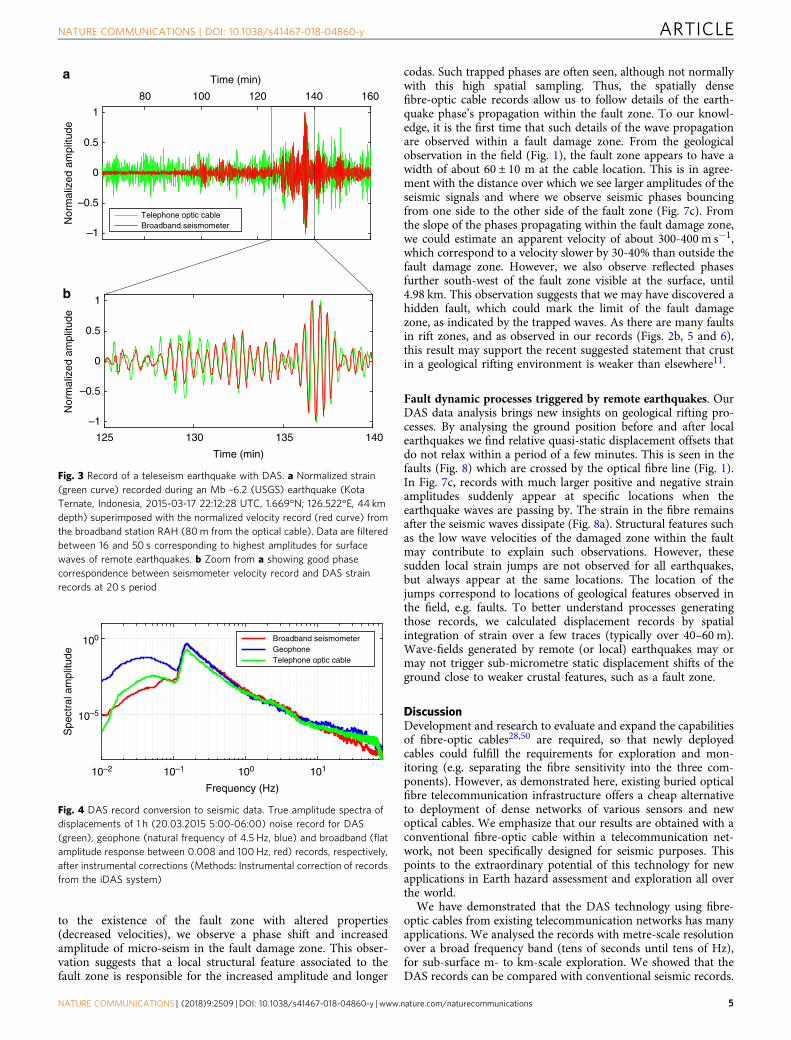
We identify signals generated from a large variety of bothanthropogenic and natural sources (0.05 Hz up to >100 Hz).High frequency signals (1–100 Hz) are mostly generated byanthropogenic sources, such as passing cars, fluid circulating inpipes of nearby geothermal power stations, hammer shots on theground, people walking, and distant active explosion shots(Figs. 2–4). In addition, we detected local earthquakes(0.5–20 Hz) associated with the seismic activity of the Mid-Atlantic Ridge (Supplementary Table 1). We observed oceanicmicro-seism (ambient seismic noise with signal frequencies from0.1 to several Hz), as well as Rayleigh waves from large remoteearthquakes (with ~20 s signal period, Fig. 3 and SupplementaryTable 2). Figure 3 shows the filtered records (range 5–40 s) fromthe optic cable and broadband seismometer for a Mb ~6.2earthquake in Indonesia, including surface waves (period ranging10–30 s).

We validate our observations with records from co-locatedshort-period three-component geophones and broadband seismicsensors deployed in the vicinity of the optic cable41 (Fig. 1;Method: Cable localisation). Waveforms from individual tracesalong the optical fibre exhibit high coherency, as well as withsignals from broadband seismometers located along the cable(stations RAH and EIN, Fig. 1). Broadband signals (0.1–10 Hz)associated with the ground deformation due to passing cars

along the fibre can be observed (Fig. 2a). We retrieve local averagesub-surface ground elastic properties from the response to a carusing simple ground deformation models (Methods).

To interpret DAS data, it is of primary importance toevaluate the performance of the iDAS system with respect totraditional acquisition seismic systems22,25–27. We compare singlerecord of the DAS data set with records from the closestgeophone and from a nearby broadband seismometer. Weperform this data comparison both on ambient noise (Fig. 4)and during earthquakes. Several technical issues must be firstsolved. (1) We locate each DAS trace along the cable with a finalspatial uncertainty of ±5 m, using hammer shots and GPSlocations from the geophone data. (Fig. 1 and Methods). (2) Weorient the recorded horizontal components of the seismometersalong the local direction given by the cable. (3) We correct theinstrumental responses of the iDAS system (Methods), of thegeophones and the broadband seismometer on the respectiverecord, prior to the determination of the seismic signal phase andamplitude.

The applied instrumental correction for the iDAS system canbe used to accurately represent amplitude and phase of theseismic signal as confirmed by the comparison to classical seismicrecording equipment (Fig. 4). Although DAS data can beconverted to ground velocity, our conversion is valid in a certainfrequency range only. Therefore, it is more convenient to follow adifferent approach when analysing fibre-optic DAS data, asdemonstrated in the analysis and modelling of the grounddeformation due to a passing car (Methods: Shallow sub-surfacecrustal properties determination). DAS systems typically measurestrain rate or strain between two neighbouring positions withinan optical fibre. The integration of strain data in space (along thecable) allows the calculation of the displacement of each datapoint relative to a chosen reference. Given an appropriateintegration length, amplitude and phase, static local deformationsand passing seismic signals can be quantified, removing the needto apply the instrumental correction. For localized deformations,the integration length must exceed the distance over which thedeformation occurs. For passing seismic waves, at least half of themaximum wavelength must be integrated to properly quantifyseismic amplitudes (Nyquist’s theorem). The required length forlong period signals easily exceeds the length of the sensor system(cable), which is typically a couple of km. While focusing onsingle traces and applying the instrumental correction isappropriate to analyse passing waves with periods from 0.01 sto several minutes, high frequency signals as well as localized(static) deformation can be accurately analysed by integratingDAS data in space. In the following, we apply time-integration ofthe strain rate to obtain strain and space-integration to obtaindisplacement (Methods: "Strain and displacement and velocitydetermination").

Earthquake identification and localisation. Accurate earthquakelocalisation is still one of the challenges in seismology42. Theaccuracy of the seismic wave velocity model and the networkdesign determine the earthquake hypocentre accuracy. Thecrustal structure of Reykjanes was the topic of investigation inseveral geophysical and particularly seismic studies43. The ECfunded project “IMAGE” performed new passive seismic dataacquisition, including deployment of Ocean Bottom Seism-ometers44. A structural analysis was performed using classical andmodern seismic methods41,45,46. In particular, we jointly invertedearthquakes locations and P-wave (Vp) and/or Vp/Vs ratio modelsof Reykjanes by a local travel time tomography41. From surfacedown to 4–5 km, seismic velocity increases rapidly from 1.8 to4.2 km s−1, which is a typical velocity gradient for oceanic crust.

–22.7° −22.5°

63.8°

63.9°

RAH

5 km

Dyke E

Curve 1Curve 2 Curve 3

Fault 1 Fault 2Fault 3

Fault 4

I c e l a n d

ReykjanesAtlanticOcean

Fault zone

EIN

Fig. 1 Location of the fibre-optic cable in Reykjanes and main geologicalfeatures70. Location of the fibre-optic cable (continuous green line) fromthe telecommunication network (Míla Company) used for ourmeasurements within the Reykjanes fissure swarm (black lines). Small lightblue squares along the fibre-optic cable represent geophones. Blue trianglesindicate broadband seismological stations from the European ProjectIMAGE (Integrated Methods for Advanced Geothermal Exploration)network41,44. RAH and EIN are the closest broadband stations to the opticalcable. The thick black lines indicate a series of cones and postglacialcraters, from the latest eruptive episode in Reykjanes in 1210–1240 (e.g.Dyke E= Eldvörp crater row). The black star indicates a local earthquakeepicentre (depth ~3.5 km). The thin red curve indicates the limit of the Sh=Sandfellshæð lava shield (most recent lava flow), hiding most of the faultsat the surface of the tip of the Peninsula. The inset represents the locationof the area in Iceland (North Atlantic), with black dots being epicentres of68 earthquakes (Supplementary Table 1) recorded during the 9 days of ouroptical DAS records

NATURE COMMUNICATIONS | DOI: 10.1038/s41467-018-04860-y ARTICLE

NATURE COMMUNICATIONS | (2018) 9:2509 | DOI: 10.1038/s41467-018-04860-y | www.nature.com/naturecommunications 3

Vp/Vs ratios are indicative of the absence of large magma reser-voirs in Reykjanes, which is also confirmed by the recent IDDP-2drilling47.

We focus here on one particular earthquake (Ml ~1.2) thatoccurred almost beneath the cable at 3 ± 1 km depth in thetomographic model41. Figure 5 shows the geophone and DASrecords along the cable for this small local earthquake. We use anautomatic picker based on Akaike Information Criteria to obtainmore than 500 valid P- and S-wave arrival times along the cable.P-wave picks have good coherency between neighbouring traceswhereas S-wave have poorer coherency (Fig. 6). Although thetelecommunication cable geometry was for sure not designed forearthquake monitoring, we obtain a hypocentre location using P-and S-wave travel times automatically picked on all tracesrecorded along the cable. We find a hypocentre similar to the oneobtained from conventional seismological network41. The prob-ability density function (pdf) of the earthquake hypocentrelocation is obtained using only the travel time data derived fromthe DAS record (Supplementary Figure 7). The pdf locates thehypocentre within few hundred metres from the hypocentrelocation obtained in the IMAGE velocity model demonstratingthat the iDAS system can be used for earthquake monitoring andlocalization. In addition, we note the rather good match both inamplitude and trend between the derived Vp/Vs ratio obtainedfrom DAS records for this earthquake (only one) and the Vp/Vs

ratio from 3D local tomography (Fig. 6b).

Crustal structural features detection. Geometrical and physicalsub-surface properties of the damage fault zone could be derivedusing waves from local earthquakes trapped within a fault damagezone (Fig. 7). From the geological and structural maps of Rey-kjanes48, we notice that the fibre-optic cable crosses several tec-tonic and volcanic features, i.e. volcanic dykes and faults. Oneprominent fault zone crosses the cable at a distance of about 5 kmalong the road (Fig. 1). This fault zone crops out along the rift tothe north and the south of the road over several kilometres. TheEldvörp crater row crosses the cable at a distance of about10.5 km. Several observations indicate the signature of those

geological features in the DAS record. For example, in Figs. 5band 6a note the larger delay of P-wave arrival time at distance~5 km, corresponding to the presence of a fault zone. Similarly,note the faster arrival times at distance ~10.5 km, where the cablecrosses the Eldvörp crater row. In Fig. 5d, Vp/Vs ratio along thecable shows kinks located at faults. Those features cannot be seenin the sparser geophone records.

Dense arrays of seismometers give the opportunity to betterimage the sub-surface, especially using recently developedimaging techniques, such as ambient noise cross-correlationand auto-correlation technologies49. Even when classical sources(earthquakes, etc.) are absent, we show that ambient noiseanalysis techniques reveal wave disturbances associated with faultzones (Method: Ambient noise interferometric techniques withDAS records). As ambient noise is rather strong in Reykjanes45,we computed autocorrelations and cross-correlations in order toillustrate the detection and imaging capabilities of those methodswith DAS records (Supplementary Figure 8). We observe similarquality and good coherency between autocorrelations from DASrecord and co-located geophones and the classical X shape ofwave propagation from the virtual source towards larger offsets.Those results demonstrate that geophysical studies (detection,mapping, localisation, monitoring, etc.) from correlations meth-ods could be performed using available telecommunication cablenetworks for further structural interpretation.

Towards imaging the damage zone within fault systems. Fromthe analysis of trapped waves in fault damage zones, P-wave andS-wave velocities were found to be typically 35 to 45% lower thanthose of the surroundings rocks in California7. For all earth-quakes recorded by the iDAS system, we observed similar char-acteristic wave-field features at several places along thetelecommunication cable. As an example, we focus on a faultdamage zone (FDZ) with a clear surface expression (Fig. 7). Weobserve an increase in both, duration and amplitude of trappedwaves excited by local earthquakes. Interestingly, we observesimilar trapped-wave features in the micro-seismic noise, evenwhen local earthquakes are absent (Supplementary Figure 9). Due

50 100 150 200

Time (s)

3

4

5

6

7

8

9

10

11

12D

ista

nce

(km

)

Earthquake

Car

3

4

5

6

7

8

9

10

11

Dis

tanc

e (k

m)

20 40 60 80 100 120

Time (s)

–6

–5

–4

–3

–2

–1

0

1

2

3

4

5

6

Nan

ostr

ain

Fault 1

Fault zoneCurve 1

Fault 2

Curve 2

Fault 3Curve 3

Dyke

Fault 4

a b

Fig. 2 DAS records. a 4min of strain signal (17 March 2015, 12:33–12:37). Only selected normalized traces (one trace out of 25, i.e. one trace every 100m,frequency range 0.01–100 Hz) are shown. A local earthquake is revealed by higher frequencies in the signal from 135 to 140 s. Coherent oscillations of5–6 s period correspond to ocean-driven micro-seism. Traces between 10.5 and 11.6 km with large amplitude signals correspond to a car travelling on theroad along the cable (Methods: Shallow sub-surface crustal properties determination). b 2 min of strain record (19.03.2015, 15:27 UTC) showing micro-seism (4–6 s period) propagating from the south coast northwards along the cable. Beamforming computation (from the DAS record) indicates a source inthe Atlantic Ocean, SW of Iceland. Changes in cable direction along the road (black labels) induce a change in the incidence angle of the micro-seismwaves, and therefore amplitude change. Amplitudes and phases are disturbed at specific locations (indicated by the red labels), which correspond togeological features such as faults or volcanic dykes (Fig. 1)

ARTICLE NATURE COMMUNICATIONS | DOI: 10.1038/s41467-018-04860-y

4 NATURE COMMUNICATIONS | (2018) 9:2509 | DOI: 10.1038/s41467-018-04860-y | www.nature.com/naturecommunications

to the existence of the fault zone with altered properties(decreased velocities), we observe a phase shift and increasedamplitude of micro-seism in the fault damage zone. This obser-vation suggests that a local structural feature associated to thefault zone is responsible for the increased amplitude and longer

codas. Such trapped phases are often seen, although not normallywith this high spatial sampling. Thus, the spatially densefibre-optic cable records allow us to follow details of the earth-quake phase’s propagation within the fault zone. To our knowl-edge, it is the first time that such details of the wave propagationare observed within a fault damage zone. From the geologicalobservation in the field (Fig. 1), the fault zone appears to have awidth of about 60 ± 10 m at the cable location. This is in agree-ment with the distance over which we see larger amplitudes of theseismic signals and where we observe seismic phases bouncingfrom one side to the other side of the fault zone (Fig. 7c). Fromthe slope of the phases propagating within the fault damage zone,we could estimate an apparent velocity of about 300-400 m s−1,which correspond to a velocity slower by 30-40% than outside thefault damage zone. However, we also observe reflected phasesfurther south-west of the fault zone visible at the surface, until4.98 km. This observation suggests that we may have discovered ahidden fault, which could mark the limit of the fault damagezone, as indicated by the trapped waves. As there are many faultsin rift zones, and as observed in our records (Figs. 2b, 5 and 6),this result may support the recent suggested statement that crustin a geological rifting environment is weaker than elsewhere11.

Fault dynamic processes triggered by remote earthquakes. OurDAS data analysis brings new insights on geological rifting pro-cesses. By analysing the ground position before and after localearthquakes we find relative quasi-static displacement offsets thatdo not relax within a period of a few minutes. This is seen in thefaults (Fig. 8) which are crossed by the optical fibre line (Fig. 1).In Fig. 7c, records with much larger positive and negative strainamplitudes suddenly appear at specific locations when theearthquake waves are passing by. The strain in the fibre remainsafter the seismic waves dissipate (Fig. 8a). Structural features suchas the low wave velocities of the damaged zone within the faultmay contribute to explain such observations. However, thesesudden local strain jumps are not observed for all earthquakes,but always appear at the same locations. The location of thejumps correspond to locations of geological features observed inthe field, e.g. faults. To better understand processes generatingthose records, we calculated displacement records by spatialintegration of strain over a few traces (typically over 40–60 m).Wave-fields generated by remote (or local) earthquakes may ormay not trigger sub-micrometre static displacement shifts of theground close to weaker crustal features, such as a fault zone.

DiscussionDevelopment and research to evaluate and expand the capabilitiesof fibre-optic cables28,50 are required, so that newly deployedcables could fulfill the requirements for exploration and mon-itoring (e.g. separating the fibre sensitivity into the three com-ponents). However, as demonstrated here, existing buried opticalfibre telecommunication infrastructure offers a cheap alternativeto deployment of dense networks of various sensors and newoptical cables. We emphasize that our results are obtained with aconventional fibre-optic cable within a telecommunication net-work, not been specifically designed for seismic purposes. Thispoints to the extraordinary potential of this technology for newapplications in Earth hazard assessment and exploration all overthe world.

We have demonstrated that the DAS technology using fibre-optic cables from existing telecommunication networks has manyapplications. We analysed the records with metre-scale resolutionover a broad frequency band (tens of seconds until tens of Hz),for sub-surface m- to km-scale exploration. We showed that theDAS records can be compared with conventional seismic records.

10–2 10–1 100 101

Frequency (Hz)

10–5

100

Spe

ctra

l am

plitu

de

Broadband seismometerGeophoneTelephone optic cable

Fig. 4 DAS record conversion to seismic data. True amplitude spectra ofdisplacements of 1 h (20.03.2015 5:00-06:00) noise record for DAS(green), geophone (natural frequency of 4.5 Hz, blue) and broadband (flatamplitude response between 0.008 and 100 Hz, red) records, respectively,after instrumental corrections (Methods: Instrumental correction of recordsfrom the iDAS system)

80 100 120 140 160

Time (min)

–1

–0.5

0

0.5

1

Nor

mal

ized

am

plitu

de

Telephone optic cableBroadband seismometer

125 130 135 140

Time (min)

–1

–0.5

0

0.5

1

Nor

mal

ized

am

plitu

dea

b

Fig. 3 Record of a teleseism earthquake with DAS. a Normalized strain(green curve) recorded during an Mb ~6.2 (USGS) earthquake (KotaTernate, Indonesia, 2015-03-17 22:12:28 UTC, 1.669°N; 126.522°E, 44 kmdepth) superimposed with the normalized velocity record (red curve) fromthe broadband station RAH (80m from the optical cable). Data are filteredbetween 16 and 50 s corresponding to highest amplitudes for surfacewaves of remote earthquakes. b Zoom from a showing good phasecorrespondence between seismometer velocity record and DAS strainrecords at 20 s period

NATURE COMMUNICATIONS | DOI: 10.1038/s41467-018-04860-y ARTICLE

NATURE COMMUNICATIONS | (2018) 9:2509 | DOI: 10.1038/s41467-018-04860-y | www.nature.com/naturecommunications 5

We report applications focussing on sub-surface exploration forelastic rock properties and earthquake monitoring. We also dis-covered unusual wave-field features of fault structures anddynamics in a geological active rift (Reykjanes, Iceland). Thespatial density increase over a long distance is one of the majoradvantages for obtaining detailed information on Earth propertydistribution. With only one earthquake (we did not use otherearthquakes), we determined structural rock properties at the kmscale and at the fault damage zone scale and inferred hints onstrain accumulation and creeping processes. For instance, thetrapped seismic phases observed in a fault damage zone aresingle- or multiple- reflected phases at two reflectors or more,which we interpret as being fault zone boundaries, defining thefault damage zone, as inferred from our seismic observations.Reflected waves in the micro-seism suggest that seismic energy istrapped in the fault zone at various frequencies. Those resultssuggest that when applied to many earthquakes, even moredetailed information could be retrieved. Our observations alsoreveal potential creeping processes at faults and fault damagezones induced by impinging seismic waves from local earth-quakes. Dynamic strain perturbations due to the passing wavesfrom local earthquakes trigger relative displacements that maycorrespond to tiny aseismic fault movements, interpreted ascreeping processes. Micro-seism may influence fault creepingprocesses as well as remote earthquakes. Further analysis in thisdirection could help solve questions related to co-seismic faultdeformation3,10,51, understand fault preparation prior to largeearthquakes as well as aseismic deformation. Those results open anew window for the study of remote triggering of earthquakesand stress build-up at faults, especially in cities where fibre-opticcable networks may be dense and where seismic hazard is high(San Francisco, Mexico, Tokyo, etc).

The dramatic increase in sensor density over a large distancewith unprecedented acquisition characteristics (sampling in spaceand time and over a large frequency band) suggests that scientistscould test new approaches and unconventional data processing,which then might obtain more accurate results compared toclassical seismological methods. The DAS technology thus offersa great potential for Earth exploration and natural hazardassessment, offering new scientific research opportunities.Improving the sensitivity of cables in existing networks, deter-mining accurate position and orientation of the observed tracesand understanding details of the ground/cable coupling issues25

are certainly great challenges when exploiting buried opticalcommunication lines. For the situation on Reykjanes Peninsula,the analysis of the stress transfer from the ground to the sensingcore of the fibre is more than 90% efficient for seismic frequenciesbetween several 10’s Hz and long seismic periods52. By demon-strating that the data acquired on a telecommunication networkof fibre-optic cable fulfills many requirements for improvement ofseismological analysis, we foresee a vibrant future for the use ofoptical sensor technologies in seismology applications. Besidesthe deployment of new dedicated and improved cables in order toallow for observation of the full strain tensor, existing infra-structures may allow for simultaneous monitoring of strain andground motion for natural hazard assessment. They could help inmore accurate earthquake localisation and focal mechanismdetermination, volcanic activity monitoring and a morecomplete characterisation of the range of volcanic and seismic

Tim

e (s

)Distance (km)

3 4 5 6 8 10 11 12

b

1

2

3

4

P

S

a

3

1

2

4Geophone velocity

Fibre optic strain

Distance (km)

3 4 5 6 7 8 10 11 129

7 9

Fig. 5 Records of a local earthquake. a Geophone record (blue) of an Ml ~1.2local earthquake (23.03.2015, 16:07:08.5 U.T.C.—Iceland MeteorologicalOffice) and fibre-optic (green) record at the corresponding locations of thegeophone. b DAS record of the same earthquake as in a

Vp/V

s

1.7

1.8

1.6

1.9

1.5

Distance (km)

2 3 4 5 6 8 10 11

a1

2

3

Fibre optic P-pick

Geophone P-pick

Synthetic P-arrival

Fibre optic S-pick

Synthetic S-arrival

Geophone S-pick

b7 9

Fig. 6 Exploration studies using conventional seismological methods and afibre-optic telecommunication line. a P- and S-waves’ travel timesautomatically picked along the profile: each symbol represents a P- (blackstar) and S- (grey dots) arrival times on the DAS records. The whitesquares with black dot and the white circle with black dot correspond to P-and S-wave travel times, respectively, picked on the geophone records withthe same automatic picker. The continuous grey (black) lines correspond totheoretical arrival times for the inverted hypocentre using P- and S-wavepicks from the cable (respectively). b Observed Vp/Vs ratio computed at alltraces and compared with the results obtained from the travel timetomography (green dots) obtained from more than 2000 local earthquakesover 1.5 years41. The black line corresponds to the polynomial(Savitsky–Golay) smoothing filter of order 5 with size frame ~3 km longthrough the fibre-optic Vp/Vs individual values

ARTICLE NATURE COMMUNICATIONS | DOI: 10.1038/s41467-018-04860-y

6 NATURE COMMUNICATIONS | (2018) 9:2509 | DOI: 10.1038/s41467-018-04860-y | www.nature.com/naturecommunications

sources, seismic hazard assessment, global seismology studies,exploration, etc.

We also suggest that our results may open the door to newways of data processing53. With the advent of spatially un-aliased,i.e. densely sampled seismic data, array analysis methods (e.g.Helmholtz tomography) becomes easier to implement54, poten-tially providing a huge improvement in resolution by directlyinverting and/or imaging sub-surface structures utilizing fullwave-field recordings.

Can we also envisage a change of paradigm in theoreticalseismology? The classical stress/displacement approach in seis-mology uses the basics of mechanics and observational seismol-ogy is based mostly on displacement and/or velocity and/oracceleration sensor recordings. With a fibre-optic cable providingequivalent broadband seismometers records, the gradient of thedisplacement, i.e. the strain, is uniquely measured at many morelocations than before. We believe new processing methods may beneeded. New mathematical progress for tomography has beenrecently discovered55 but their application is hindered by the lackof information at the Earth surface56. Since fibre-optic lines aredeployed very widely and densely on Earth, e.g. for tele-communication (~106 km cable deployed under the sea57), weanticipate that our results will open a new era for strain andground-motion acquisition at all scales, for both seismic proces-sing and modelling. For instance and non-exclusively, monitoringof underground explosions in the framework of the CTBTO,volcano monitoring, seismic hazard assessment, landslide

monitoring and, global seismology using transatlantic opticalcables could benefit from this technology with current and futureinfrastructures. We may also envisage dedicated experiments tocompare new instrument development in rotational seismology58,and detailed studies of surface wave properties59. Many otherapplications, like car traffic monitoring, theft protection, cityunderground monitoring37 will promote telecommunicationcompanies as actors for Earth hazard monitoring, exploration andsecurity enhancement for the benefit of research60 and humansocieties.

MethodsDistributed fibre-optic strain sensing. Various optical architectures have beenused to interrogate the backscattered Rayleigh light, ranging from relatively simple,coherent-OTDR (optical time domain reflectometer) schemes, which are unable todetermine acoustic phase and so are unsuitable for seismic measurements, to morecomplex arrangements which provide the full acoustic amplitude, frequency andphase. Both the simple and complex range of systems are generally described asDAS25,33 or DVS26, though only the phase sensitive variants have been successfullyused for seismic applications60. The description of the underlying sensing princi-ples of the DAS/DVS technology has been reported22,61,62. When a laser pulse islaunched into an optical fibre, a fraction of the light is elastically scattered (Rayleighscattering) due to random inhomogeneity distribution in the glass fibre material.During interrogation of an optical fibre, the backscattered photons can be detected.The position of the scattering inhomogeneity within the fibre can be calculatedbased on the speed of light within the fibre. This method is called optical timedomain reflectometry (OTDR)63. If a coherent laser pulse is launched into the fibre,with appropriate optical processing, not only the amplitude but also the phase ofthe backscattered photons can be analysed (phase-OTDR). For any section of thefibre, the phase-difference Δϕ of photons scattered at both ends of that section is

100 m

Faul

t zon

e

Telephone

line

5.04 km

5.09 km

4.98 km4.8 4.9 5

5.1

5.2

Distance (km)

P

S

Tim

e (s

)

Reflections

0

6

1

5

4

3

2

a

b c

Fau

ltzo

ne

5.1

Fig. 7 Structure of a fault damage zone within an active geological rift. a The road and the cable (distance ~5 km) cross several faults, e.g. a clearly visiblefault zone with more loose material in the field (between 5.04 and 5.09 km). b The fault damage zone is visible by the ~50–60m wide depression area(picture taken at ~100m SW of the road, looking towards SW). Note that at the cable location no depression area is visible. The depression is only thesurface expression at the position of the picture (Picture Martin Lipus, GFZ). c Short record (6 s) of strain phases from a local earthquake (Fig. 5) trapped inthe fault damage zone. Phases are reflected until ~4.98 km, which may indicate a hidden fault with surface expression. Waves inside and outside the faultzone have different apparent velocities

NATURE COMMUNICATIONS | DOI: 10.1038/s41467-018-04860-y ARTICLE

NATURE COMMUNICATIONS | (2018) 9:2509 | DOI: 10.1038/s41467-018-04860-y | www.nature.com/naturecommunications 7

linearly related to the length of this section27. When the section of the sensing fibreis unperturbed, the length and, consequently, the phase-difference Δϕ remainsunchanged. Any perturbation inducing a strain ε on the fibre will change thatdifference. The strain rate can therefore be mapped along the sensing fibre byexamining the changes in the phase of the elastically backscattered photonsbetween successive measurements. For example, an imbalanced Mach-Zehnderinterferometer has been used to measure dynamic strain changes along the fibre64.A fibre-optic cable can hence be considered a system consisting of a large numberof one component relative strain gauges. State of the art DAS systems are capable ofquantifying the frequency, amplitude, phase and location of dynamic perturbationsanywhere along the sensing fibre. Measurement systems with the capability toresolve perturbations of 40 nϵ are reported27.

Strain and displacement and velocity determination. In our study, we define theDAS system as comprising the deployed fibre-optic cable (sensor) and the iDASinterrogation system33. The phase-difference is a measure of the relative travel timeand hence the relative distance. The physical distance over which the phase-difference measurement is performed, is referred to as the “gauge length” dx26,61.Comparing successive pulses, phase changes are directly related to the distancechanges and therefore the strain rate in direction of the fibre can be recorded. Inthe iDAS system, each digital sample is indexed by the centre location of a movingwindow along a cable’s fibre core (the sample’s ‘channel’, x) and recording time(the sample’s ‘time’, t). Thus, if u(x,t) represents the dynamic displacement of thefibre, the DAS observation DASobs at axial location x and time t is a measure of thestrain rate at the distance x from the iDAS recorder and is expressed by:

DAS obsðx; tÞ ¼ u x þ dx2; t

� �� u x � dx

2; t

� �� �

� u x þ dx2; t � dt

� �� u x � dx

2; t � dt

� �� � ð1Þ

where dx and dt are the spatial gauge length and temporal sample interval,respectively. The typical gauge length for seismic applications spans dx= ~10 m.The longer the gauge length, the more sensitive the DAS system with increasedsignal to noise ratio. Wavelength λ below dx/2 can however not be resolved(Nyquist’s theorem in space26). Together with the spatial sampling, the gaugelength determines the dependency between individual seismic traces. Althoughdata can be acquired with a high spatial resolution, the assumption of independenttraces only holds true if the gauge length of neighbouring traces does not overlap.In order to achieve a sufficient intensity of the backscattered light for each datapoint and every laser pulse, the laser pulse has a given width and the backscatteredlight has to be integrated for a given time. Both, the pulse width as well as theintegration time acts as a moving averaging filtering in space26. In some imple-mentations, post-acquisition averaging of individual traces is applied to suppressunwanted optical noise and an increase in seismic signal/noise ratio.

DAS data can be equivalently regarded either as an estimate of the fibre strain-rate

∂

∂t∂u∂x

� �ð2Þ

or as an estimate of the spatial derivative of fibre particle velocity

∂

∂x∂u∂t

� �ð3Þ

If we integrate the distributed strain-rate along the optical fibre with respect totime, local strain can be estimated for every section along the optical fibre. If weintegrate the local strain with respect to space, the relative displacement can becalculated at all points along the profile. Note that by differentiating with respect totime, we obtain an estimate of the velocity of the ground, which we may compare

–300

–200

–100 0

100

200

300

Nanometers

Tim

e (s

)

Fau

ltzo

ne

–100

0

100

200

4.8 4.9 5 5.1 5.2

Distance (km)

–100 –8

0

–60

–40

–20 0 20 40 60 80 100

Nanostrain

Fau

ltzo

ne

–100

0

100

200

4.8 4.9 5 5.1 5.2

Distance (km)

EqS

udde

nst

rain

ste

p

a b

Fig. 8 Dynamics of a fault damage zone within an active geological rift. a Extensive record (400 s) of strain observed in the vicinity of the damage faultzone, from 100 s before, during and 300 s after the earthquake (Figs. 6 and 7). Sudden strain steps (black arrows indicated at the time 0) occur overseveral neighbouring traces simultaneously to the waves of the earthquake. Strain remains with the same value for at least 300 s, possibly more. Thelocation of the steps correspond to locations of geological features observed in the field, e.g. faults. b Displacement computed by spatial integration atselected traces along the same section of the cable as in Fig. 7a and c. The displacement is directly obtained from the spatial integration of the strain ina over a 60-m-long sliding window. Eq: earthquake

ARTICLE NATURE COMMUNICATIONS | DOI: 10.1038/s41467-018-04860-y

8 NATURE COMMUNICATIONS | (2018) 9:2509 | DOI: 10.1038/s41467-018-04860-y | www.nature.com/naturecommunications

to local broadband seismometer records. We compare spectral data indisplacements (Fig. 4).

Cable localisation. Using an optical cable at the surface is driven by the idea thatthere could potentially be a larger range of applications both in hazard assessmentand crustal exploration, although applications at the surface are described to bemore challenging26. Instead of deploying a new dedicated cable (with great amountof expenses), we use an optical fibre within the commercial telecommunicationnetwork on the Reykjanes peninsula, SW-Iceland. The geographical position of thecable was provided by the telecommunication provider (Mila). The optical data isgiven in terms of distance along the optical fibre within the cable to the iDASrecorder. Each trace of the DAS record has an associated distance from the iDASrecorder. In order to locate and check the accuracy of the observed distances fromthe DAS record, we deployed an array of 33 geophones every 250–500 m along thecable. We determine the position of each geophone using precise differential GPS(accuracy better than ~0.5 m). To locate individual DAS traces, we assign thegeographical position of the geophones to the closest optical trace. At each geo-phone, we performed six successive hammer shots for calibration purpose. Wecompare DAS records of hammer shots in the vicinity of each geophone with therecords of these shots at different traces along the cable. We identify the DAS tracewith the earliest arrival time of seismic waves associated to the hammer shots. Forevery geophone position, the shortest distance to the position of the cable wascalculated and the geographical position of this point assigned to the identifiedDAS trace. In between individual reference points, the geographical position waslinearly interpolated along the cable. To verify the positions of the traces in theintervals between geophones, the distance between individual DAS traces is cal-culated using the number of traces and the distance along the cable and given bythe geophone localisation. We are able to localize every shot with an accuracy ofthe sampling resolution along the optical fibre (i.e. 4 m). The localization accuracyfor records located in the range over which geophones were deployed, is thereforein the order of 10 m for distant traces to the next shot point. The sensitivity of alinear fibre is decreasing with increasing angle of the incident wave with respect tothe cable direction. Therefore, the comparison of the DAS data with other type ofrecords (geophone and broadband seismometer) requires the projection of seismicmotions (displacement, velocity or acceleration) in the local direction of the cable.We oriented the broadband sensors using an Octans (IXSEA) gyro-compass65.

Shallow sub-surface crustal properties determination. The iDAS system is ableto record the ground deformation associated to cars passing by along the cable(Fig. 2a and Supplementary Fig. 6). We use here those records to locally determineaverage rock properties beneath the road. To predict the deformation of the groundto the car’s weight, we model the car by a series of 4 point loads moving onan isotropic semi-infinite elastic half-space66. As the speed of the car is slowcompared to the Rayleigh wave velocity in the ground, we use theFlamant–Boussinesq approximation theory describing the static deformation of apoint load on the ground surface67. In this theory, the ground displacement u(ux,uy,uz) in the ith direction is given by

ui ¼F4πμ

x3xir3

þ 3� 4υð Þ δi3r� 1� 2υð Þ

r þ x3δ3i þ

xir

� �� �ð4Þ

where F is the force of the point load (weight of the car), μ the shear modulus of the

rock, υ the Poisson ratio, r ¼ffiffiffiffiffiffiffiffiffiffiffiffiffiffiffiffiffiffiffiffiffiffiffiffiffiffiu2x þ u2y þ u2z

q, and δ is the Kronecker sign (Einstein

notation). The centre of mass of the car (we computed 4 mass contributions at thelocations of the 4 wheels) is assumed to be located at a constant distance of 2.5 mfrom the cable. The shape of the strain trace with time at one location is dependenton the speed and weight of the car, on the distance to the cable, and on the elasticproperties of the ground, e.g. P-wave velocity. Supplementary Fig. 6 shows anexample of ground property determination with this approach at one locationalong the cable. The best match of the deformation curve we found for a carmoving at ~25 km h−1 with a sub-surface P-wave velocity of ~750 m s−1. Note thealmost perfect match between observations and our simple prediction. The P-wavevelocity is consistent with velocities obtained (~500–1000m s−1) from the refrac-tion analysis of the seismic waves generated by hammer test shots68. We could usethis method to derive a profile of sub-surface velocities long the cable, a task thatwe will pursue in a further study.

Instrumental correction of records from the iDAS system. The iDAS systemmeasures strain rate (Methods: Strain and displacement and velocity determina-tion). In order to calibrate the amplitude and phase responses of the recordedsignal by the iDAS system, an impulse displacement signal is sent in the cable andthe output strain is measured at different frequencies. The amplitude and phaseresponses both depend on the frequency (Supplementary Figure 1). To retrieve thetrue amplitude over a frequency band of interest (<100 Hz) for our seismicapplications, we should correct the recorded signal from the amplitude and phaseshift introduced by the recording unit (iDAS). We focus only on the frequency ofinterest for our seismological applications: from <0.01 Hz to 100 Hz. In this fre-quency band, the response can be modelled with simple functions. We first dealwith the dependency of the instrumental wave response with an apparent ground

velocity v. The response of the iDAS is better expressed in apparent wavelength λalong the cable. As v= λf, f being the frequency, we can express the response as anon-velocity dependent function with the wavelength (Supplementary Fig. 2): thegain and phase responses are the same for all wave velocities. We also notice thatthe amplitude response is linear with wavelengths above roughly 20 m. The seismicfrequencies of interest are about <100 Hz, therefore wavelengths of interest for usare above 15–50 m depending on the ground velocity. A simplified instrumentalresponse can be used. We note that the amplitude decay with diminishing fre-quency is almost linear below 100 Hz (in logarithm versus logarithm scales). Wealso note that the phase is almost constant below 10–20 Hz (in semi-logarithmscale). We express both amplitude and phase responses as a linear function of thewavelength or frequency. We correct from the recorded signals for the iDASinstrumental response by multiplying, in the Fourier domain, the amplitude by thesimple function C*λ, C being a constant. If we apply the correction to theinstrumental response, we can calibrate this constant to C= 0.0159, by imposingthe corrected instrumental response to amplitude 1 for the frequencies of interest,as shown in Supplementary Fig. 3. We also note that the phase shift is constant π/2for long wavelengths (above 100 m). In practice, the processing steps to performthe restitution of the “true” ground motion, consists of integrating strain rate intostrain, as iDAS records data as strain rate, and as the instrumental response isexpressed in strain. We assume that the initial strain is zero all along the cable, onthe basis that the average strain along the cable is zero. Then, the correction isapplied in the frequency domain as shown in Supplementary Fig. 4. The restitutiondepends on the velocity of the medium. Supplementary Fig. 5 shows smoothedversion of the restitution spectra for different velocities. Differences are due todifferent amplitude and phase responses of the instrumental correction at differentvelocities. Note that the transfer function that we used is valid only for the gaugelength used (10 m).

Probability density function of an earthquake location. The probability densityfunction is, in inversion theory, a way to represent the difference between obser-vations and a model. In order to find the hypocentre location that minimises themisfit difference between the synthetic travel times and DAS observations in theleast square sense (RMS), we performed systematic computation of synthetic traveltimes for many hypothetic hypocentres within a 3D grid around the hypocentrelocation found by the 3D tomographic velocity model in Reykjanes. Each hypo-thetic hypocentres give a misfit value with respect to observations, represented inthe Supplementary Fig. 7. The DAS cable observations are sufficient to define anarea where the true hypocentre might be. The minimum misfit value is found at alocation which is at <1 km from the hypocentre determined from the 3D traveltime tomography.

Ambient noise interferometric techniques with DAS records. We used ambientnoise interferometric techniques to generate source gathers by cross-correlatingDAS records at different positions (Supplementary Fig. 8). Results indicate mostlyone-sided correlation because ambient noise has a strong directivity, the sourcesbeing located in the Atlantic Ocean (South-Western). Strong perturbation ofambient noise amplitude occurs at the location of fault damage zones. Other dis-turbances in the signal amplitude and phase (Supplementary Fig. 8) reveal variousfeatures visible in the field (such as directional changes of the cable at curves of theroad), but also other features that we cannot identify accurately, without more fieldinspection. An example of auto-correlation computed at specific DAS/DVSrecords, corresponding to the location of the geophones and along the wholeprofile are shown in Supplementary Fig. 8b and c.

Data availability. The fibre-optic data and the geophone datasets69 generated andanalysed in the current study and that supports the finding of this study areaccessible via the data repository of “GFZ Data Services” (https://doi.org/10.5880/GFZ.6.2.2018.003).

Received: 28 November 2017 Accepted: 21 May 2018

References1. Sigmundsson, F. et al. Segmented lateral dyke growth in a rifting event at

Bárðarbunga volcanic system, Iceland. Nature 517, 191–195 (2015).2. Witze, A. Volcano risk quantified. Nature 519, 16–17 (2015).3. Harris, R. H. Large earthquakes and creeping faults. Rev. Geophys. 55, 169–198

(2017).4. Budd, G. Efficient interpretation. New Technol. Mag. 1–2 (2010).5. Yatman, G., Üzumcü, S., Pahsa, A. & Mert, A. A. Intrusion detection sensors

used by electronic security systems for critical facilities and infrastructures: areview. WIT Trans. Built Environ. 151, 131–141 (2015).

6. Shelef, E. & Oskin, M. Deformation processes adjacent to active faults:examples from eastern California. J. Geophys. Res. 115, B05308 (2010).

NATURE COMMUNICATIONS | DOI: 10.1038/s41467-018-04860-y ARTICLE

NATURE COMMUNICATIONS | (2018) 9:2509 | DOI: 10.1038/s41467-018-04860-y | www.nature.com/naturecommunications 9

7. Li, Y. in Seismic Imaging Fault Damage and Heal (ed Li, Y.) Ch 4, 378 pp(Walter de Gruyter GmbH & Co KG, High Education Press, 2014).

8. Amitrano, D. Rupture by damage accumulation in rocks. Int. J. Fract. 139,369–381.

9. Jousset, P. & Rohmer, J. Evidence of remotely triggered micro-earthquakesduring salt cavern collapse. Geophys. J. Int 191, 207–223 (2012).

10. Duan, B., Kang, J. & Li, Y.-G. Deformation of compliant fault zones inducedby nearby earthquakes: theoretical investigations in two dimensions. J.Geophys. Res. 116, B03307 (2011).

11. Thun, J. et al. Micrometre-scale deformation observations reveal fundamentalcontrols on geological rifting. Nat., Sci. Rep. 6, 36676 (2016).

12. Allen, R. M. Transforming earthquake detection? Science 225, 297–298 (2012).13. Burdick, S. et al. Upper mantle heterogeneity beneath North America from

travel time tomography with global and US Array Transportable Array data.Seismol. Res. Lett. 79, 384–392 (2008).

14. Hansen, S. M. & Schmandt, B. Automated detection and location ofmicroseismicity at Mount St. Helens with a large-N geophone array. Geophys.Res. Lett. 42, 7390–7397 (2015).

15. Sigloch, K., McQuarrie, N. & Nolet, G. Two-stage subduction history underNorth America inferred from multiple-frequency tomography. Nat. Geosci. 1,458–462 (2008).

16. Snieder, R. & Wapenaar, K. Imaging with ambient noise. Phys. Today 2010,44–49 (2010).

17. Elliott, J. R., Walters, R. J. & Wright, T. J. The role of space-based observationin understanding and responding to active tectonics and earthquakes. Nat.Commun. 7, 13844 (2017).

18. Houlié, N. et al. New approaches to detect seismic surface waves in 1 Hz-samples GPS time series. Nat. Sci. Rep. 1, 1–9 (2011).

19. Lehujeur, M., Vergne, J., Schmittbuhl, J. & Maggi, A. Characterization ofambient seismic noise near a deep geothermal reservoir and implications forinterferometric methods: a case study in northern Alsace, France. Geotherm.Energy 3, 3 (2015).

20. Matias, I., Ikezawa, S. & Corres, J. Fiber Optic Sensors—Current Status andFuture Possibilities 381 (Springer, Switzerland, 2017).

21. Coutant, O., De Mangin, M. & Le Coarer, E. Fabry–Perrot Optical strain-meter with an embeddable, low-power interrogation system. Optica 2,400–404 (2015).

22. Masoudi, A. & Newson, T. P. Contributed review: distributed optical fibredynamic strain sensing. Rev. Sci. Instrum. 87, 011501 (2016).

23. Nickès, M. & Ravet, F. Distributed fibre sensors: depth and sensitivity. Nat.Photonics 4, 431–432 (2010).

24. Philen, D. L., White, I. A., Kuhl, J. F. & Mettler, S. Single-mode fibre ODTR:experiment and theory. IEEE J. Quantum Electron. QE18 10, 1499–1508 (1982).

25. Willis, M. E. et al. Quantitative quality of distributed acoustic sensing verticalseismic profile data. Leading Edge 35, 605–609 (2016).

26. Dean, T., Cuny, T. & Hartog, A. H. The effect of gauge length on axiallyincident P-waves measured using fibre optic distributed vibration sensing.Geophys. Prospect. 65, 184–193 (2016).

27. Masoudi, A. & Newson, T. P. High spatial resolution distributed optical fibredynamic strain sensor with enhanced frequency and strain resolution. OpticLett. 42, 290–293 (2017).

28. Kuvshinov, B. N. Interaction of helically wound fibre-optic cables with planeseismic waves. Geophys. Prospect. 64, 671–688 (2016).

29. Cox, B. et al. Distributed acoustic sensing for geophysical measurement,monitoring and verification. CSEG Recorder 37, 7–13 (2012).

30. Hartog, A., Frignet, B., Mackie, D. & Clark, M. Vertical seismic opticalprofiling on wireline logging cable. Geophys. Prospect. 62, 1365–2478 (2014).

31. Madsen, K. N., Tondel, R. & Kvam, O. Data-driven depth calibration fordistributed acoustic sensing. Leading Edge 35, 610–614 (2016).

32. Daley, T. et al. Field testing of fibre-optic distributed acoustic sensing (DAS)for sub-surface seismic monitoring. Leading Edge 36, 936–942 (2013).

33. Parker, T., Shatalin, S. & Farhadiroushan, M. Distributed acoustic sensing—anew tool for seismic applications. First Break 32, 61–69 (2014).

34. Jousset, P., Reinsch, T., Henninges, J., Blanck, H. & Ryberg, T. Strain andground-motion monitoring at magmatic areas: ultra-long and ultra-densenetworks using fibre optic sensing systems. Geophys. Res. Abstr. 18,EGU2016–EGU15707 (2016).

35. Reinsch, T., Jousset, P., Henninges, J. & Blanck, H. Distributed acousticsensing technology in magmatic geothermal areas—first results from asurvey in Iceland. In Proc. European Geothermal Congress, Strasbourg, France(2016).

36. Becker, M. W., Ciervo, C., Cole, M., Coleman, T. & Mondanos, M. Fracturehydromechanical response measured by fiber optic distributed acousticsensing at milliHertz frequencies. Geophys. Res. Lett. 44, 7295–7302 (2017).

37. Dou, S. et al. Distributed acoustic sensing for seismic monitoring of the nearsurface: a traffic-noise interferometry. Sci. Rep. 7, 11620 (2017).

38. Lindsey, N. J. et al. Fiber-optic network observations of earthquake wavefields.Geophs. Res. Lett. 44, 1944–8007 (2017).

39. Martin, E. R., Biondi, B. L., Karrenbach, M. & Cole, S. Continuous subsurfacemonitoring by passive seismic with distributed acoustic sensors—the“Stanford Array” experiment. In First EAGE Workshop on Practical ReservoirMonitoring. https://doi.org/10.3997/2214-4609.201700017 (2017).

40. Franklin, J. B. A. et al. Dark Fiber and Distributed Acoustic Sensing:Applications to Monitoring Seismicity and Near Surface Properties (AGUGeneral Assembly, New Orleans, 2017).

41. Jousset, P. et al. Seismic tomography in Reykjanes, SW Iceland. In ExtendedAbstract EGC, Strasbourg (2016).

42. Geiger, L. Probability method for the determination of earthquakes epicentresfrom arrival time only. Bull. St. Louis Univ. 8, 60–71 (1912).

43. Weir, N. R. W. et al. Crustal structure of the northern Reykjanes Ridge andReykjanes Peninsula, southwest Iceland. J. Geophys. Res. 106, 6347–6368(2001).

44. Blanck, H., Jousset, P., Ágústsson, K., Hersir, G. P. & Flóvenz Ó. G. Analysis ofseismological data on Reykjanes peninsula, Iceland. In Extended AbstractEGC, Strasbourg (2016).

45. Verdel A. et al. Reykjanes ambient noise reflection interferometry. In Proc.European Geothermal Congress, Strasbourg, France (2016).

46. Weemstra C. et al. Time-lapse seismic imaging of the Reykjanes geothermalreservoir. In Proc. European Geothermal Congress, Strasbourg, France (2016).

47. Friðleifsson, G. O. et al. ICDP supported coring in IDDP-2 at Reykjanes—theDEEPEGS demonstrator in Iceland—supercritical conditions reached below4.6 km depth. Geophys. Res. Abstr. 19, EGU2017-14147-1 (2017).

48. Saemundsson, K. & Einarsson, S. Geological Map of Iceland, Sheet 3, SW-Iceland 2nd edn (Museum of Natural History and the Iceland GeodeticSurvey, Reykjavík, 1980).

49. Ryberg, T., Muksin, U. & Bauer, K. Ambient seismic noise tomography revealsa hidden caldera and its relation to the Tarutung pull-apart basin at theSumatran Fault Zone, Indonesia. J. Volcanol. Geotherm. Res. 321, 73–84(2016).

50. Wright, L. G., Christodoulides, D. N. & Wise, F. W. Controllable spatio-temporal non-linear effects in multi-mode fibres Nat. Photon. 9, 306–310(2015).

51. Nissen, E., Maruyama, T., Parker, T., Arrowsmith, J. R. & Elliot, J. Coseismicfault zone deformation revealed with differential lidar: examples fromJapanese Mw~7 intraplate earthquakes. Earth Planet. Sci. Lett. 405, 244–256(2014).

52. Reinsch, T., Thurley, T. & Jousset, P. On the coupling of a fiber optic cableused for distributed acoustic/vibration sensing applications—a theoreticalconsideration. Meas. Sci. Technology 28, 12 (2017).

53. Weemstra, C. et al. Application of seismic interferometry by multidimensionaldeconvolution to ambient noise recorded in Malargüe, Argentina. Geophys. J.Int. 208, 693–714 (2017).

54. Lin, F. C. & Ritzwoller, M. H. Helmholtz surface wave tomography forisotropic and azimuthally anisotropic structure. Geophys. J. Int. 186,1104–1120 (2011).

55. Stefanov, P., Uhlmann, G. & Vasy, A. Local and local boundary rigidity andthe geodesic X-ray transform in the normal gauge. Preprint at https://arxiv.org/abs/1702.03638v2 (2017).

56. Castelvecchi, D. Long-sought maths proof can shape-up seismology. Nature542, 281–282 (2017).

57. ICPC. International Cable Protection Committee. https://www.iscpc.org/cable-data. Accessed 2017.

58. Lee, W. H. K., Igel, H. & Trifunac, M. D. Recent advances in rotationalseismology. Seismol. Res. Lett. 80, 479–490, (2009).

59. Colombi, A., Guenneau, S., Roux, P. & Craster, R. V. Transformationseismology: composite soil lenses for steering surface wave elastic Rayleighwaves. Nat. Sci. Rep. 6, 25320 (2016).

60. You, Y. Harnessing telecoms cables for science. Nature 466, 690–691(2010).

61. Masoudi, A., Belal, M. & Newson, T. P. A distributed optical fibre dynamicstrain sensor based on phase-OTDR. Meas. Sci. Technol. 24, 085204 (2013).

62. Daley, T., Miller, D. E., Dodds, K., Cook, P. & Freifield, B. M. Field testing ofmodular borehole monitoring with simultaneous acoustic sensing andgeophone vertical seismic profiles at Citronelle, Alabama. Geophys. Prospect.12,1318–1334 (2016).

63. Barnoski, J. K. & Jensen, S. M. Fibre waveguides: a novel technique forinvestigating attenuation characteristics. Appl. Opt. 15, 2112–2115 (1976).

64. Posey, R. J., Johnson, G. A. & Vohra, S. T. Strain sensing based oncoherent Rayleigh scattering in an optical fibre. Electron. Lett. 36, 1688–1689(2000).

65. Schreiber, K. U., Velikoseltsev, A., Carr, A. J. & Franco-Anaya, R. Theapplication of fibre optic gyroscopes for the measurement of rotations instructural engineering. Bull. Seism. Soc. Am. 99, 1207–1214 (2009).

66. Liou, J. Y. & Sung, J. C. Surface responses induced by point load or uniformtraction moving steadily on an anisotropic half-plane. Int. J. Solids Struct. 45,2737–2757 (2008).

ARTICLE NATURE COMMUNICATIONS | DOI: 10.1038/s41467-018-04860-y

10 NATURE COMMUNICATIONS | (2018) 9:2509 | DOI: 10.1038/s41467-018-04860-y | www.nature.com/naturecommunications

67. Fung, Y. C. Foundations of Solid Mechanics (Prentice-Hall, EnglandwoodCliffs, 1965).

68. Raab, T., Reinsch, T., Jousset, P. & Krawczyk, C. Multi-station analysisof surface wave dispersion using distributed acoustic sensing. InEAGE/DGG Workshop on Fibre Optic Technology, Potsdam, 31 March 2017(2017).

69. Jousset, P. et al Fibre-optic data set from Reykjanes Iceland. V. 1.0. GFZ DataServices. https://doi.org/10.5880/GFZ.6.2.2018.003 (2018).

70. Generic Mapping Tools. http://gmt.soest.hawaii.edu. (Last accessed: June, 4th,2018).

AcknowledgementsWe gratefully acknowledge help of the following people and institutions; Ernst Huenges,David Bruhn, Christian Haberland, Kemal Erbas, Karl-Heinz Jäckel and Arthur Jolly forfruitful discussions; Míla (Iceland) during the field implementation; ISOR staff andUniversity students for helping with the geophone and broadband sensors deployment.HS Orka gave access to the road along the telephone line. Geophones, broadbandseismometers and data logger equipment are from the Geophysical Instrumental Pool ofPotsdam (GIPP). Map in Fig. 1 was produced using the Generic Mapping Tool v5.0. Thiswork received funding from the European Union Seventh Framework Programme underthe Grant No. 608553 (project IMAGE), from the Iceland Geosurvey, the Geo-ForschungZentrum Potsdam and the Helmholtz Association.

Author contributionsP.J. guided the whole experiment and wrote the first manuscript draft and the finalversion of the manuscript. P.J., Th.R., J.H., H.B. designed, planned the experiment andperformed the field measurements. P.J., Th.R., T.R. and H.B. analysed the data. P.J. andTh.R. produced most results shown in the manuscript. T.R. produced the noise corre-lation results. R.A. and A.C. produced the instrumental response for iDAS technology.G.P.H. supported the operational and organisational aspects in Iceland and helped in thefield. G.P.H., M.W. and C.M.K. supported the initial idea and gave strong input in the

interpretation and future perspectives. P.J. and Th.R. wrote the manuscript. C.K.improved it. A.C. checked for English.

Additional informationSupplementary Information accompanies this paper at https://doi.org/10.1038/s41467-018-04860-y.

Competing interests: The authors declare no competing interests.

Reprints and permission information is available online at http://npg.nature.com/reprintsandpermissions/

Publisher's note: Springer Nature remains neutral with regard to jurisdictional claims inpublished maps and institutional affiliations.

Open Access This article is licensed under a Creative CommonsAttribution 4.0 International License, which permits use, sharing,

adaptation, distribution and reproduction in any medium or format, as long as you giveappropriate credit to the original author(s) and the source, provide a link to the CreativeCommons license, and indicate if changes were made. The images or other third partymaterial in this article are included in the article’s Creative Commons license, unlessindicated otherwise in a credit line to the material. If material is not included in thearticle’s Creative Commons license and your intended use is not permitted by statutoryregulation or exceeds the permitted use, you will need to obtain permission directly fromthe copyright holder. To view a copy of this license, visit http://creativecommons.org/licenses/by/4.0/.

© The Author(s) 2018

NATURE COMMUNICATIONS | DOI: 10.1038/s41467-018-04860-y ARTICLE

NATURE COMMUNICATIONS | (2018) 9:2509 | DOI: 10.1038/s41467-018-04860-y | www.nature.com/naturecommunications 11