Dynamic Programming Strikes Back

Guido MoerkotteUniversity of MannheimMannheim, Germany

moerkotte@informatik.uni-mannheim.de

Thomas NeumannMax-Planck Institute for Informatics

Saarbrücken, Germanyneumann@mpi-inf.mpg.de

ABSTRACTTwo highly efficient algorithms are known for optimally or-dering joins while avoiding cross products: DPccp, which isbased on dynamic programming, and Top-Down PartitionSearch, based on memoization. Both have two severe limi-tations: They handle only (1) simple (binary) join predicatesand (2) inner joins. However, real queries may contain com-plex join predicates, involving more than two relations, andouter joins as well as other non-inner joins.

Taking the most efficient known join-ordering algorithm,DPccp, as a starting point, we first develop a new algorithm,DPhyp, which is capable to handle complex join predicatesefficiently. We do so by modeling the query graph as a (vari-ant of a) hypergraph and then reason about its connectedsubgraphs. Then, we present a technique to exploit this ca-pability to efficiently handle the widest class of non-innerjoins dealt with so far. Our experimental results show thatthis reformulation of non-inner joins as complex predicatescan improve optimization time by orders of magnitude, com-pared to known algorithms dealing with complex join pred-icates and non-inner joins. Once again, this gives dynamicprogramming a distinct advantage over current memoizationtechniques.

Categories and Subject DescriptorsH.2 [Systems]: Query processing

General TermsAlgorithms, Theory

1. INTRODUCTIONFor the overall performance of a database management

system, the cost-based query optimizer is an essential pieceof software. One important and complex problem any cost-based query optimizer has to solve is to find the optimaljoin order. In their seminal paper, Selinger et al. not onlyintroduced cost-based query optimization but also proposed

Permission to make digital or hard copies of all or part of this work forpersonal or classroom use is granted without fee provided that copies arenot made or distributed for profit or commercial advantage and that copiesbear this notice and the full citation on the first page. To copy otherwise, torepublish, to post on servers or to redistribute to lists, requires prior specificpermission and/or a fee.SIGMOD’08, June 9–12, 2008, Vancouver, BC, Canada.Copyright 2008 ACM 978-1-60558-102-6/08/06 ...$5.00.

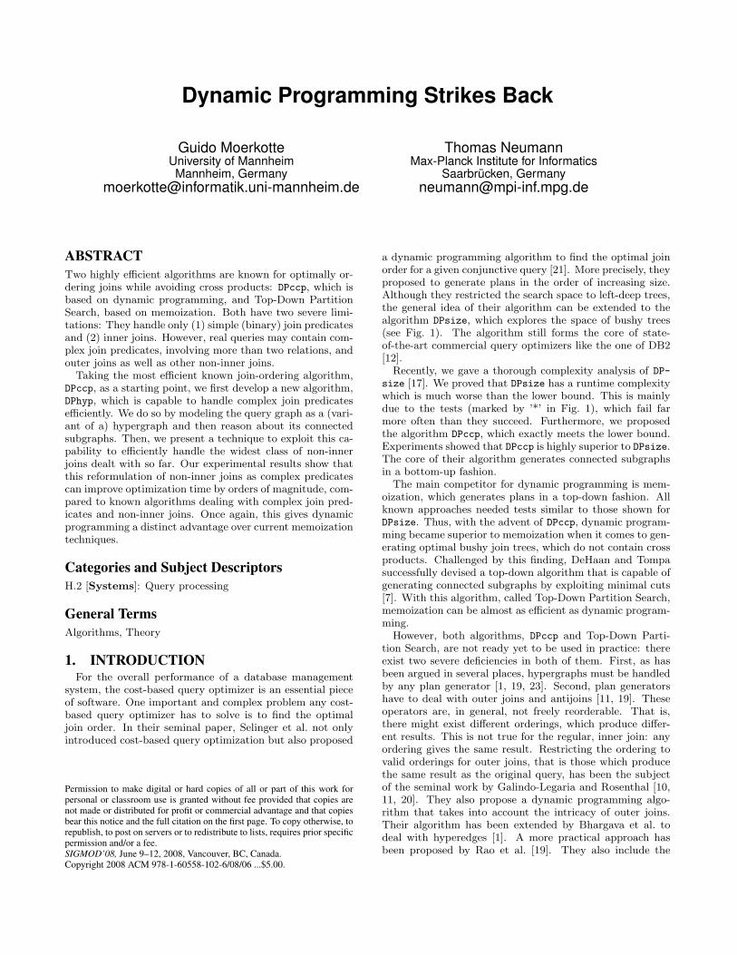
a dynamic programming algorithm to find the optimal joinorder for a given conjunctive query [21]. More precisely, theyproposed to generate plans in the order of increasing size.Although they restricted the search space to left-deep trees,the general idea of their algorithm can be extended to thealgorithm DPsize, which explores the space of bushy trees(see Fig. 1). The algorithm still forms the core of state-of-the-art commercial query optimizers like the one of DB2[12].

Recently, we gave a thorough complexity analysis of DP-

size [17]. We proved that DPsize has a runtime complexitywhich is much worse than the lower bound. This is mainlydue to the tests (marked by ’*’ in Fig. 1), which fail farmore often than they succeed. Furthermore, we proposedthe algorithm DPccp, which exactly meets the lower bound.Experiments showed that DPccp is highly superior to DPsize.The core of their algorithm generates connected subgraphsin a bottom-up fashion.

The main competitor for dynamic programming is mem-oization, which generates plans in a top-down fashion. Allknown approaches needed tests similar to those shown forDPsize. Thus, with the advent of DPccp, dynamic program-ming became superior to memoization when it comes to gen-erating optimal bushy join trees, which do not contain crossproducts. Challenged by this finding, DeHaan and Tompasuccessfully devised a top-down algorithm that is capable ofgenerating connected subgraphs by exploiting minimal cuts[7]. With this algorithm, called Top-Down Partition Search,memoization can be almost as efficient as dynamic program-ming.

However, both algorithms, DPccp and Top-Down Parti-tion Search, are not ready yet to be used in practice: thereexist two severe deficiencies in both of them. First, as hasbeen argued in several places, hypergraphs must be handledby any plan generator [1, 19, 23]. Second, plan generatorshave to deal with outer joins and antijoins [11, 19]. Theseoperators are, in general, not freely reorderable. That is,there might exist different orderings, which produce differ-ent results. This is not true for the regular, inner join: anyordering gives the same result. Restricting the ordering tovalid orderings for outer joins, that is those which producethe same result as the original query, has been the subjectof the seminal work by Galindo-Legaria and Rosenthal [10,11, 20]. They also propose a dynamic programming algo-rithm that takes into account the intricacy of outer joins.Their algorithm has been extended by Bhargava et al. todeal with hyperedges [1]. A more practical approach hasbeen proposed by Rao et al. [19]. They also include the

DPsize (R = {R0, . . . , Rn−1})for ∀ Ri ∈ R dpTable[{Ri}] = Ri

for ∀ 1 < s ≤ n ascending // size of planfor ∀ 1 ≤ s1 < s // size of left subplan

for ∀ S1 ⊂ R : |S1| = s1, S2 ⊂ R : |S2| = s− s1

if S1 ∩ S2 6= ∅ continue (*)if ¬(S1 connected to S2) continue (*)p =dpTable[S1]B dpTable[S2]if cost(p)<cost(dpTable[S1 ∪ S2])

dpTable[S1 ∪ S2] = preturn dpTable[{R0, . . . , Rn−1}]

Figure 1: Algorithm DPsize

R1

R2

R3

R4

R5

R6

Figure 2: Sample hypergraph

antijoin. All these approaches use DPsize as their startingpoint. Thus, they suffer from a much higher than necessaryruntime complexity.

In this paper, we introduce DPhyp, which can efficientlydeal with hypergraphs (Sec. 2 and 3). Experiments will showthat it is highly superior to existing approaches (Sec. 4). In asecond step, we deal with left and full outer joins, antijoins,nestjoins, and their dependent counterparts (Section 5). Itwill be shown that non-inner joins can be dealt with byintroducing new hyperedges. Thus, no extension to DPhyp

except for calculating the new hyperedges is necessary todeal with a complete set of non-inner and dependent joins.This approach is highly superior to existing approaches evenif no initial hyperedges are present, i.e. the query exhibitsonly simple predicates but non-inner joins.

2. HYPERGRAPHS

2.1 DefinitionsLet us start with the definition of hypergraphs.

Definition 1 (hypergraph). A hypergraph is a pairH = (V, E) such that

1. V is a non-empty set of nodes and

2. E is a set of hyperedges, where a hyperedge is an un-ordered pair (u, v) of non-empty subsets of V (u ⊂ Vand v ⊂ V ) with the additional condition that u∩v = ∅.

We call any non-empty subset of V a hypernode. We as-sume that the nodes in V are totally ordered via an (arbi-trary) relation ≺. The ordering on nodes is important forour algorithm.

A hyperedge (u, v) is simple if |u| = |v| = 1. A hypergraphis simple if all its hyperedges are simple.

Note that a simple hypergraph is the same as an ordinaryundirected graph. In our context, the nodes of hypergraphs

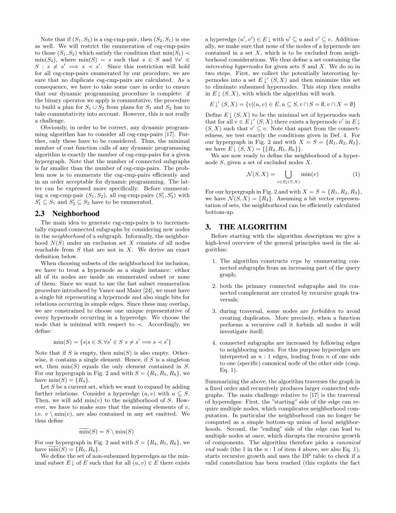
are relations and the edges are abstractions of join predi-cates. Consider, for example, a join predicate of the formR1.a + R2.b + R3.c = R4.d + R5.e + R6.f . This predi-cate will result in a hyperedge ({R1, R2, R3}, {R4, R5, R6}).Fig. 2 contains an example of a hypergraph. The set V ofnodes is V = {R1, . . . , R6}. Concerning the node order-ing, we assume that Ri ≺ Rj ⇐⇒ i < j. There are thesimple edges ({R1}, {R2}), ({R2}, {R3}), ({R4}, {R5}), and({R5}, {R6}). The hyperedge from above is the only truehyperedge in the hypergraph.

Note that is possible to rewrite the above complex joinpredicate. For example, it is equivalent to R1.a + R2.b =R4.d + R5.e + R6.f −R3.c. This leads to a hyperedge({R1, R2}, {R3, R4, R5, R6}). If the query optimizer is ca-pable of performing this kind of algebraic transformations,all derived hyperedges are added to the hypergraph, at leastconceptually. We will come back to this issue in Section 6.

To decompose a join ordering problem represented as ahypergraph into smaller problems, we need the notion ofsubgraph. More specifically, we only deal with node-inducedsubgraphs.

Definition 2 (subgraph). Let H = (V, E) be a hy-pergraph and V ′ ⊆ V a subset of nodes. The node in-duced subgraph G|V ′ of G is defined as G|V ′ = (V ′, E′)with E′ = {(u, v)|(u, v) ∈ E, u ⊆ V ′, v ⊆ V ′}. The nodeordering on V ′ is the restriction of the node ordering of V .

As we are interested in connected subgraphs, we give

Definition 3 (connected). Let H = (V, E) be a hy-pergraph. H is connected if |V | = 1 or if there exists a par-titioning V ′, V ′′ of V and a hyperedge (u, v) ∈ E such thatu ⊆ V ′, v ⊆ V ′′, and both G|V ′ and G|V ′′ are connected.

If H = (V, E) is a hypergraph and V ′ ⊆ V is a subsetof the nodes such that the node-induced subgraph G|V ′ isconnected, then we call V ′ a connected subgraph or csg forshort. The number of connected subgraphs is importantfor dynamic programming: it directly corresponds to thenumber of entries in the dynamic programming table. If anode set V ′′ ⊆ (V \V ′) induces a connected subgraph G|V ′′ ,we call V ′′ a connected complement of V ′ or cmp for short.

Within this paper, we will assume that all hypergraphsare connected. This way, we can make sure that no crossproducts are needed. However, when dealing with hyper-graphs, this condition can easily be assured by adding ac-cording hyperedges: for every pair of connected components,we can add a hyperedge whose hypernodes contain exactlythe relations of the connected components. By consideringthese hyperedges as B operators with selectivity 1, we getan equivalent connected hypergraph (i.e., one that describesthe same query).

2.2 Csg-cmp-pairWith these notations, we can move closer to the heart of

dynamic programming by defining a csg-cmp-pair.

Definition 4 (csg-cmp-pair). Let H = (V, E) be ahypergraph and S1, S2 two subsets of V such that S1 ⊆ Vand S2 ⊆ (V \S1) are a connected subgraph and a connectedcomplement. If there further exists a hyperedge (u, v) ∈ Esuch that u ⊆ S1 and v ⊆ S2, we call (S1, S2) a csg-cmp-pair.

Note that if (S1, S2) is a csg-cmp-pair, then (S2, S1) is oneas well. We will restrict the enumeration of csg-cmp-pairsto those (S1, S2) which satisfy the condition that min(S1) ≺min(S2), where min(S) = s such that s ∈ S and ∀s′ ∈S : s 6= s′ =⇒ s ≺ s′. Since this restriction will holdfor all csg-cmp-pairs enumerated by our procedure, we aresure that no duplicate csg-cmp-pairs are calculated. As aconsequence, we have to take some care in order to ensurethat our dynamic programming procedure is complete: ifthe binary operator we apply is commutative, the procedureto build a plan for S1 ∪ S2 from plans for S1 and S2 has totake commutativity into account. However, this is not reallya challenge.

Obviously, in order to be correct, any dynamic program-ming algorithm has to consider all csg-cmp-pairs [17]. Fur-ther, only these have to be considered. Thus, the minimalnumber of cost function calls of any dynamic programmingalgorithm is exactly the number of csg-cmp-pairs for a givenhypergraph. Note that the number of connected subgraphsis far smaller than the number of csg-cmp-pairs. The prob-lem now is to enumerate the csg-cmp-pairs efficiently andin an order acceptable for dynamic programming. The lat-ter can be expressed more specifically. Before enumerat-ing a csg-cmp-pair (S1, S2), all csg-cmp-pairs (S′1, S

′2) with

S′1 ⊆ S1 and S′2 ⊆ S2 have to be enumerated.

2.3 NeighborhoodThe main idea to generate csg-cmp-pairs is to incremen-

tally expand connected subgraphs by considering new nodesin the neighborhood of a subgraph. Informally, the neighbor-hood N(S) under an exclusion set X consists of all nodesreachable from S that are not in X. We derive an exactdefinition below.

When choosing subsets of the neighborhood for inclusion,we have to treat a hypernode as a single instance: eitherall of its nodes are inside an enumerated subset or noneof them. Since we want to use the fast subset enumerationprocedure introduced by Vance and Maier [24], we must havea single bit representing a hypernode and also single bits forrelations occurring in simple edges. Since these may overlap,we are constrained to choose one unique representative ofevery hypernode occurring in a hyperedge. We choose thenode that is minimal with respect to ≺. Accordingly, wedefine:

min(S) = {s|s ∈ S,∀s′ ∈ S s 6= s′ =⇒ s ≺ s′}

Note that if S is empty, then min(S) is also empty. Other-wise, it contains a single element. Hence, if S is a singletonset, then min(S) equals the only element contained in S.For our hypergraph in Fig. 2 and with S = {R4, R5, R6}, wehave min(S) = {R4}.

Let S be a current set, which we want to expand by addingfurther relations. Consider a hyperedge (u, v) with u ⊆ S.Then, we will add min(v) to the neighborhood of S. How-ever, we have to make sure that the missing elements of v,i.e. v \ min(v), are also contained in any set emitted. Wethus define

min(S) = S \min(S)

For our hypergraph in Fig. 2 and with S = {R4, R5, R6}, wehave min(S) = {R5, R6}.

We define the set of non-subsumed hyperedges as the min-imal subset E ↓ of E such that for all (u, v) ∈ E there exists

a hyperedge (u′, v′) ∈ E ↓ with u′ ⊆ u and v′ ⊆ v. Addition-ally, we make sure that none of the nodes of a hypernode arecontained in a set X, which is to be excluded from neigh-borhood considerations. We thus define a set containing theinteresting hypernodes for given sets S and X. We do so intwo steps. First, we collect the potentially interesting hy-pernodes into a set E ↓′ (S, X) and then minimize this setto eliminate subsumed hypernodes. This step then resultsin E ↓ (S, X), with which the algorithm will work.

E ↓′ (S, X) = {v|(u, v) ∈ E, u ⊆ S, v ∩ S = ∅, v ∩X = ∅}

Define E ↓ (S, X) to be the minimal set of hypernodes suchthat for all v ∈ E ↓′ (S, X) there exists a hypernode v′ in E ↓(S, X) such that v′ ⊆ v. Note that apart from the connect-edness, we test exactly the conditions given in Def. 4. Forour hypergraph in Fig. 2 and with X = S = {R1, R2, R3},we have E ↓ (S, X) = {{R4, R5, R6}}.

We are now ready to define the neighborhood of a hyper-node S, given a set of excluded nodes X.

N (S, X) =[

v∈E↓(S,X)

min(v) (1)

For our hypergraph in Fig. 2 and with X = S = {R1, R2, R3},we have N (S, X) = {R4}. Assuming a bit vector represen-tation of sets, the neighborhood can be efficiently calculatedbottom-up.

3. THE ALGORITHMBefore starting with the algorithm description we give a

high-level overview of the general principles used in the al-gorithm:

1. The algorithm constructs ccps by enumerating con-nected subgraphs from an increasing part of the querygraph;

2. both the primary connected subgraphs and its con-nected complement are created by recursive graph tra-versals;

3. during traversal, some nodes are forbidden to avoidcreating duplicates. More precisely, when a functionperforms a recursive call it forbids all nodes it willinvestigate itself;

4. connected subgraphs are increased by following edgesto neighboring nodes. For this purpose hyperedges areinterpreted as n : 1 edges, leading from n of one sideto one (specific) canonical node of the other side (cmp.Eq. 1).

Summarizing the above, the algorithm traverses the graph ina fixed order and recursively produces larger connected sub-graphs. The main challenge relative to [17] is the traversalof hyperedges: First, the ”starting” side of the edge can re-quire multiple nodes, which complicates neighborhood com-putation. In particular the neighborhood can no longer becomputed as a simple bottom-up union of local neighbor-hoods. Second, the ”ending” side of the edge can lead tomultiple nodes at once, which disrupts the recursive growthof components. The algorithm therefore picks a canonicalend node (the 1 in the n : 1 of item 4 above, see also Eq. 1),starts recursive growth and uses the DP table to check if avalid constellation has been reached (this exploits the fact

that DP strategies enumerate subsets before supersets). Wenow discuss the details of the algorithm.

We give the implementation of our join ordering algorithmfor hypergraphs by means of pseudocode for member func-tions of a class DPhyp. This allows us to minimize the num-ber of parameters by assuming that the query hypergraph(G = (V, E)) and the dynamic programming table (dpTable)are class members.

The whole algorithm is distributed over five subroutines.The top-level routine Solve initializes the dynamic program-ming table with access plans for single relations and thencalls EmitCsg and EnumerateCsgRec for each set containingexactly one relation. The member function EnumerateCs-

gRec is responsible for enumerating connected subgraphs.It does so by calculating the neighborhood and iteratingover each of its subset. For each such subset S1, it callsEmitCsg. This member function is responsible for findingsuitable complements. It does so by calling EnumerateCm-

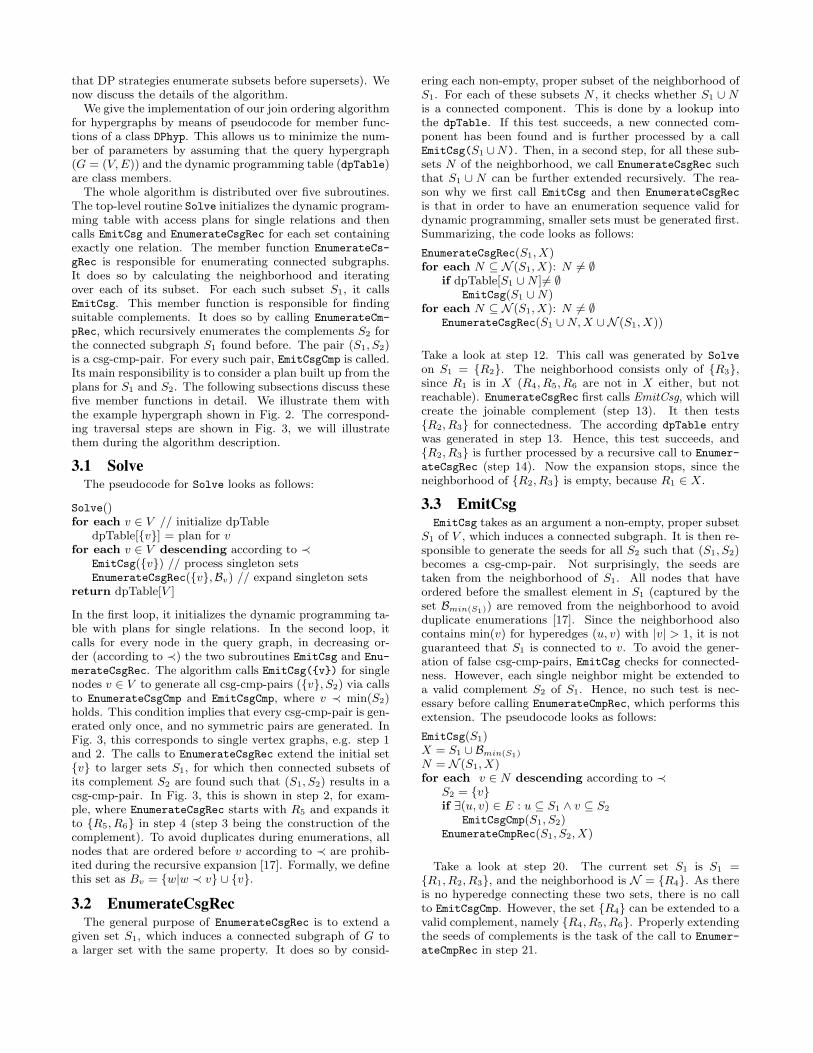
pRec, which recursively enumerates the complements S2 forthe connected subgraph S1 found before. The pair (S1, S2)is a csg-cmp-pair. For every such pair, EmitCsgCmp is called.Its main responsibility is to consider a plan built up from theplans for S1 and S2. The following subsections discuss thesefive member functions in detail. We illustrate them withthe example hypergraph shown in Fig. 2. The correspond-ing traversal steps are shown in Fig. 3, we will illustratethem during the algorithm description.

3.1 SolveThe pseudocode for Solve looks as follows:

Solve()for each v ∈ V // initialize dpTable

dpTable[{v}] = plan for vfor each v ∈ V descending according to ≺

EmitCsg({v}) // process singleton setsEnumerateCsgRec({v},Bv) // expand singleton sets

return dpTable[V ]

In the first loop, it initializes the dynamic programming ta-ble with plans for single relations. In the second loop, itcalls for every node in the query graph, in decreasing or-der (according to ≺) the two subroutines EmitCsg and Enu-

merateCsgRec. The algorithm calls EmitCsg({v}) for singlenodes v ∈ V to generate all csg-cmp-pairs ({v}, S2) via callsto EnumerateCsgCmp and EmitCsgCmp, where v ≺ min(S2)holds. This condition implies that every csg-cmp-pair is gen-erated only once, and no symmetric pairs are generated. InFig. 3, this corresponds to single vertex graphs, e.g. step 1and 2. The calls to EnumerateCsgRec extend the initial set{v} to larger sets S1, for which then connected subsets ofits complement S2 are found such that (S1, S2) results in acsg-cmp-pair. In Fig. 3, this is shown in step 2, for exam-ple, where EnumerateCsgRec starts with R5 and expands itto {R5, R6} in step 4 (step 3 being the construction of thecomplement). To avoid duplicates during enumerations, allnodes that are ordered before v according to ≺ are prohib-ited during the recursive expansion [17]. Formally, we definethis set as Bv = {w|w ≺ v} ∪ {v}.

3.2 EnumerateCsgRecThe general purpose of EnumerateCsgRec is to extend a

given set S1, which induces a connected subgraph of G toa larger set with the same property. It does so by consid-

ering each non-empty, proper subset of the neighborhood ofS1. For each of these subsets N , it checks whether S1 ∪ Nis a connected component. This is done by a lookup intothe dpTable. If this test succeeds, a new connected com-ponent has been found and is further processed by a callEmitCsg(S1 ∪N). Then, in a second step, for all these sub-sets N of the neighborhood, we call EnumerateCsgRec suchthat S1 ∪ N can be further extended recursively. The rea-son why we first call EmitCsg and then EnumerateCsgRec

is that in order to have an enumeration sequence valid fordynamic programming, smaller sets must be generated first.Summarizing, the code looks as follows:

EnumerateCsgRec(S1, X)for each N ⊆ N (S1, X): N 6= ∅

if dpTable[S1 ∪N ]6= ∅EmitCsg(S1 ∪N)

for each N ⊆ N (S1, X): N 6= ∅EnumerateCsgRec(S1 ∪N, X ∪N (S1, X))

Take a look at step 12. This call was generated by Solve

on S1 = {R2}. The neighborhood consists only of {R3},since R1 is in X (R4, R5, R6 are not in X either, but notreachable). EnumerateCsgRec first calls EmitCsg, which willcreate the joinable complement (step 13). It then tests{R2, R3} for connectedness. The according dpTable entrywas generated in step 13. Hence, this test succeeds, and{R2, R3} is further processed by a recursive call to Enumer-

ateCsgRec (step 14). Now the expansion stops, since theneighborhood of {R2, R3} is empty, because R1 ∈ X.

3.3 EmitCsgEmitCsg takes as an argument a non-empty, proper subset

S1 of V , which induces a connected subgraph. It is then re-sponsible to generate the seeds for all S2 such that (S1, S2)becomes a csg-cmp-pair. Not surprisingly, the seeds aretaken from the neighborhood of S1. All nodes that haveordered before the smallest element in S1 (captured by theset Bmin(S1)) are removed from the neighborhood to avoidduplicate enumerations [17]. Since the neighborhood alsocontains min(v) for hyperedges (u, v) with |v| > 1, it is notguaranteed that S1 is connected to v. To avoid the gener-ation of false csg-cmp-pairs, EmitCsg checks for connected-ness. However, each single neighbor might be extended toa valid complement S2 of S1. Hence, no such test is nec-essary before calling EnumerateCmpRec, which performs thisextension. The pseudocode looks as follows:

EmitCsg(S1)X = S1 ∪ Bmin(S1)

N = N (S1, X)for each v ∈ N descending according to ≺

S2 = {v}if ∃(u, v) ∈ E : u ⊆ S1 ∧ v ⊆ S2

EmitCsgCmp(S1, S2)EnumerateCmpRec(S1, S2, X)

Take a look at step 20. The current set S1 is S1 ={R1, R2, R3}, and the neighborhood is N = {R4}. As thereis no hyperedge connecting these two sets, there is no callto EmitCsgCmp. However, the set {R4} can be extended to avalid complement, namely {R4, R5, R6}. Properly extendingthe seeds of complements is the task of the call to Enumer-

ateCmpRec in step 21.

. .

..

R1

R2

R3

R4

R5

R6

. .

..

R1

R2

R3

R4

R5

R6

. .

..

R1

R2

R3

R4

R5

R6

. .

..

R1

R2

R3

R4

R5

R6

. .

..

R1

R2

R3

R4

R5

R6

. .

..

R1

R2

R3

R4

R5

R6

1 2 3 4 5 6

. .

..

R1

R2

R3

R4

R5

R6

. .

..

R1

R2

R3

R4

R5

R6

. .

..

R1

R2

R3

R4

R5

R6

. .

..

R1

R2

R3

R4

R5

R6

. .

..

R1

R2

R3

R4

R5

R6

. .

..

R1

R2

R3

R4

R5

R6

7 8 9 10 11 12

. .

..

R1

R2

R3

R4

R5

R6

. .

..

R1

R2

R3

R4

R5

R6

. .

..

R1

R2

R3

R4

R5

R6

. .

..

R1

R2

R3

R4

R5

R6

. .

..

R1

R2

R3

R4

R5

R6

. .

..

R1

R2

R3

R4

R5

R6

13 14 15 16 17 18

. .

..

R1

R2

R3

R4

R5

R6

. .

..

R1

R2

R3

R4

R5

R6

. .

..

R1

R2

R3

R4

R5

R6

. .

..

R1

R2

R3

R4

R5

R6

. .

..

R1

R2

R3

R4

R5

R6

. .

..

R1

R2

R3

R4

R5

R6

19 20 21 22 23 24

. .

..

R1

R2

R3

R4

R5

R6

. .

..

R1

R2

R3

R4

R5

R6

Legend:R2R1 connected subgraph R1 forbidden nodeR2R1 connected complement R1 non-forbidden node

25 26

Figure 3: Trace of algorithm for Figure 2

3.4 EnumerateCmpRecEnumerateCsgRec has three parameters. The first param-

eter S1 is only used to pass it to EmitCsgCmp. The second pa-rameter is a set S2 which is connected and must be extendeduntil a valid csg-cmp-pair is reached. Therefore, it considersthe neighborhood of S2. For every non-empty, proper subsetN of the neighborhood, it checks whether S2 ∪ N inducesa connected subset and is connected to S1. If so, we havea valid csg-cmp-pair (S1, S2) and can start plan construc-tion (done in EmitCsgCmp). Irrespective of the outcome ofthe test, we recursively try to extend S2 such that this testbecomes successful. Overall, the EnumerateCmpRec behavesvery much like EnumerateCsgRec. Its pseudocode looks asfollows:

EnumerateCmpRec(S1, S2, X)for each N ⊆ N (S2, X): N 6= ∅

if dpTable[S2 ∪N ]6= ∅ ∧∃(u, v) ∈ E : u ⊆ S1 ∧ v ⊆ S2 ∪N

EmitCsgCmp(S1, S2 ∪N)X = X ∪N (S2, X)for each N ⊆ N (S2, X): N 6= ∅

EnumerateCmpRec(S1, S2 ∪N, X)

Take a look at step 21 again. The parameters are S1 ={R1, R2, R3} and S2 = {R4}. The neighborhood consists ofthe single relation R5. The set {R4, R5} induces a connectedsubgraph. It was inserted into dpTable in step 6. However,there is no hyperedge connecting it to S1. Hence, there is nocall to EmitCsgCmp. Next is the recursive call in step 22 withS2 changed to {R4, R5}. Its neighborhood is {R6}. The set{R4, R5, R6} induces a connected subgraph. The accordingtest via a lookup into dpTable succeeds, since the accordingentry was generated in step 7. The second part of the testalso succeeds, as our only true hyperedge connects this setwith S1. Hence, the call to EmitCsgCmp in step 23 takesplace and generates the plans containing all relations.

3.5 EmitCsgCmpThe task of EmitCsgCmp(S1,S2) is to join the optimal

plans for S1 and S2, which must form a csg-cmp-pair. Forthis purpose, we must be able to calculate the proper joinpredicate and costs of the resulting joins. This requires thatjoin predicates, selectivities, and cardinalities are attachedto the hypergraph. Since we hide the cost calculations in anabstract function cost, we only have to explicitly assemblethe join predicate. For a given hypergraph G = (V, E) and

R1R0

R2

R3

R4

R6

R7

R5

R1 R2 R3 R4

R7 R8R6R5

R0

a b

Figure 4: Cycle and Star with initial hyperedge (n =8)

a hyperedge (u, v) ∈ E, we denote by P(u, v) the predicaterepresented by the hyperedge (u, v).

The pseudocode of EmitCsgCmp should look very familar:

EmitCsgCmp(S1, S2)plan1 = dpTable[S1]plan2 = dpTable[S2]S = S1 ∪ S2

p =V

(u1,u2)∈E,ui⊆SiP(u1, u2)

newplan = plan1 Bp plan2

if dpTable[S]= ∅ ∨ cost(newplan) < cost(dpTable[S])dpTable[S] = newplan

newplan = plan2 Bp plan1 // for commutative ops onlyif cost(newplan) < dpTable[S]

dpTable[S] = newplan

First, the optimal plans for S1 and S2 are recovered from thedynamic programming table. Then, we remember in S thetotal set of relations present in the plan to be constructed.The join predicate p is assembled by taking the conjunctionof the predicates of those hyperedges that connect S1 to S2.Then, the plans are constructed and, if they are cheaperthan existing plans, stored in dpTable.

The calculation of the predicate p seems to be expensive,since all edges have to be tested. However, we can attachthe set of predicates

pS = {P(u, v)|(u, v) ∈ E, u ⊆ S}

to any plan class S ⊆ V . If we represent the pS by a bitvector, then for a csg-cmp-pair we can easily calculate pS1 ∩pS2 and just consider the result.

3.6 Memory RequirementsAll dynamic programming variants DPsize, DPsub, DPccp,

and DPhyp memoize the best plan for each subset of relationsthat induces a connected subgraph of the query graph. Sincethis is the major factor in memory consumption, the memoryrequirements of all algorithms are about the same. It is onlyabout the same, because the number of bytes necessary foreach such subset may differ sligthly. For example, DPsub

needs an additional pointer to link plans of equal size.

4. EVALUATIONUnfortunately, there are no experiments on join ordering

for hypergraphs reported in the literature. Thus, we hadto invent our own experiments. The general design princi-ple of our hypergraphs used in the experiments is that we

start with a simple graph and add one big hyperedge to it.Then, we successively split the hyperedge into two smallerones until we reach simple edges. As starting points, we usethose graphs that have proven useful for the join orderingof simple graphs. In the literature, we often find the use ofchain, cycle, star, and clique queries [17]. The behavior ofjoin ordering algorithms on chains and cycles does not differmuch: the impact of one additional edge is minor. Hence,we decided to use cycles as one starting point. Star querieshave also been proven to be very useful to illustrate differentperformance behaviors of join ordering algorithms. More-over, star queries are common in data warehousing and thusdeserve special attention. Hence, we also used star queriesas a starting point. The last potential candidate are cliquequeries. However, adding hyperedges to a clique query doesnot make much sense, as every subset of relations alreadyinduces a connected subgraph. Thus, we limited our exper-iments to hypergraphs derived from cycle and star queries.

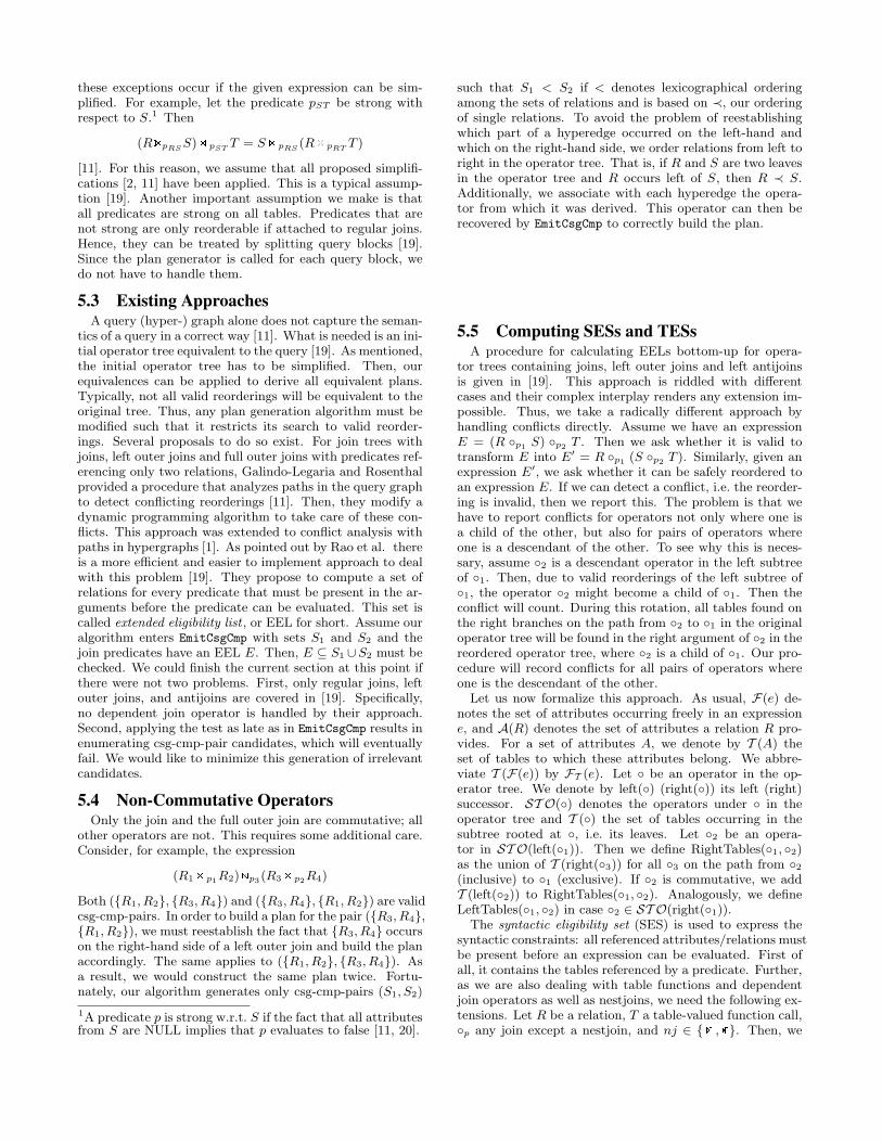
Fig. 4a shows a starting cycle-based query. It con-tains eight relations R0, . . . , R7. The simple edges are({Ri}, {Ri+1}) for 0 ≤ i ≤ 7 (with R7+1 = R0). Wethen added the hyperedge ({R0, . . . , R3}, {R4, . . . , R7}).Each of its hypernodes consists of exactly half of the re-lations. From this graph (call it G0), we derive hypergraphsG1, . . . , G3 by successively splitting the hyperedge. Thisis done by splitting each hypernode into two hypernodescomprising half of the relations. That is, apart from thesimple edges, G1 has the hyperedges ({R0, R1}, {R6, R7})and ({R2, R3}, {R4, R5}). To derive G2, we split the firsthyperedge into ({R0}, {R6}) and ({R1}, {R7}). G3 addi-tionally splits the second hyperedge into ({R2}, {R4}) and({R3}, {R5}).

For star queries, we apply the same procedure. Fig. 4bshows an initial hypergraph derived from a star. It consistsof nine relations R0, . . . , R8 and simple edges ({R0}, {Ri})for 1 ≤ i ≤ 8. The hyperedge is ({R1, . . . , R4}, {R5, . . . , R8}).More hypergraphs are generated by successively splittingthis hyperedge as described above.

4.1 The CompetitorsWe ran DPhyp against DPsize and DPsub. For regular

graphs, these algorithms are explained in detail in [17]. SinceDPsize is the most frequently used dynamic programmingalgorithm, we give its pseudocode in Fig. 1. In order todeal with hypergraphs, the pseudocode does not have tobe changed: only the second test marked by (*) has to beimplemented in such a way that it is capable to deal withhyperedges instead of only regular edges. Whereas DPsize

enumerates plans by increasing size, DPsub generates sub-sets. Assume the best plan for a set of relations S is to befound. Then DPsub generates all subsets S1 ⊂ S and joinsthe best plans for S1 and S2 = S \S1. Before doing so, thereare tests checking that (S1, S2) is a csg-cmp-pair. Again, thepseudocode of DPsub does not have to be changed, but thetest checking that S1 and S2 are connected has to be imple-mented in such a way that it can deal with hyperedges.

4.2 Cycle-Based HypergraphsFor very small queries with 3 or fewer relations, there is

no observable difference in the execution time of the differ-ent algorithms. Cycle queries with four relations exhibit asmall difference. However, since each hypernode in the ini-tial hyperedge consists of only two relations, there is only

0

0.5

1

1.5

2

2.5

0 1 2 3

op

tim

iza

tio

n t

ime

[m

s]

hyperedge splits

Cycle Queries with 8 Relations

DPhypDPsizeDPsub

0

500

1000

1500

2000

2500

3000

0 1 2 3 4 5 6 7

op

tim

iza

tio

n t

ime

[m

s]

hyperedge splits

Cycle Queries with 16 Relations

DPhypDPsizeDPsub

Figure 5: Results for cycle-based hypergraphs

one more derived hypergraph. Hence, we do not plot theruntimes but give them in tabular form. The runtime isgiven in milliseconds. The experiments were carried out ona PC with a 3.2 GHz Pentium D CPU. In the following tablewe show the result for cycles with 4 relations.

splits DPhyp DPsize DPsub

0 0.02 0.035 0.0351 0.025 0.025 0.025

Only small differences in runtime are observable here. Thischanges if we go to cycles with 8 and 16 relations. The cpu-times in milliseconds are given in the graphs in Fig. 5. Thefirst graph contains the results for cycles with 8 relations,the second one those for cycles with 16 relations. As wecan see, in all cases DPhyp is superior to any of the otheralgorithms. Further, DPsize is superior to DPsub for largequeries.

4.3 Star-Based HypergraphsLet us start by giving the results for star queries with four

satellite relations in tabular form. The table is organized thesame way as before.

splits DPhyp DPsize DPsub

0 0.03 0.085 0.0651 0.055 0.09 0.08

We already observe small runtime differences. For example,DPsize, which is used in commercial systems, is slower thanDPhyp by a factor of almost two. Further, DPsub is slightlysuperior to DPsize, but less efficient than DPhyp. For largerstar queries with eight and 16 satellite relations (see Fig. 6),these differences become rather huge. We observe that DPhypis highly superior to DPsize and DPsub. Further, DPsub issuperior to DPsize.

4.4 Queries with Regular GraphsFor completeness we also study the performance for regu-

lar graphs (i.e., simple hypergraphs without hyperedges), asthese are more common in practice and DPhyp might havelarge constants than other approaches. But the results aresimilar to the hypergraph results (see Fig. 7), DPhyp is highlysuperior to DPsize and DPsub (note the logarithmic scale).

0.001

0.01

0.1

1

10

100

1000

10000

100000

3 4 5 6 7 8 9 10 11 12 13 14 15 16

op

tim

iza

tio

n t

ime

[m

s]

number of relations

Star Queries without Hyperedges

DPhypDPsizeDPsub

Figure 7: Results for star-based regular graphs

This is also true for other graph structures, where DPhyp

performs exactly like DPccp on regular graphs.

5. NON-REORDERABLE OPERATORSThis section is organized as follows. We start with enu-

merating the set of binary operators which we handle. Then,we discuss their reorderability properties. Sec. 5.3 providesan overview of existing approaches. Problems occurring fornon-commutative operators are discussed in Sec. 5.4. Here-after, we introduce SESs and TESs, which capture possibleconflicts among operators. Finally, we discuss issues con-cerning dependent joins and show how TESs can be usedto generate the query hypergraph. An evaluation concludesthis section.

5.1 Considered Binary OperatorsLet us define the set of binary operators which we allow for

in our plans. Besides the fully reorderable join (B ), we alsoconsider the following operators with limited reorderabilitycapabilities: full outer join (M), left outer join (P), left an-tijoin (I), left semijoin (G), and left nestjoin (T ). Exceptfor the nestjoin, these are standard operators. The nestjoin(also called binary grouping or MD-join) has been proposed

0

1

2

3

4

5

6

0 1 2 3

op

tim

iza

tio

n t

ime

[m

s]

hyperedge splits

Star Queries with 8 Relations

DPhypDPsizeDPsub

0

20000

40000

60000

80000

100000

120000

0 1 2 3 4 5 6 7

op

tim

iza

tio

n t

ime

[m

s]

hyperedge splits

Star Queries with 16 Relations

DPhypDPsizeDPsub

Figure 6: Results for star-based hypergraphs

to unnest nested queries in the object-oriented [6, 22], therelational [3], and the XML context [14]. It is further usedto speed up data warehouse queries [5]. Since the variousdefinitions of the nestjoin differ slightly, we use the mostgeneral one, from which all others can be derived by spe-cialization. Let R and S be two relations, p a join predicatebetween them, ai attribute names and ei expressions in onefree variable. Then we use the following definition of thenestjoin:

RT p;[a1:e1,...,an:en]S = {r ◦ s(r)|r ∈ R}

with s(r) = [a1 : e1(g(r)), . . . , an : en(g(r))] and g(r) ={s|s ∈ S, p(r, s)}. Verbally, the operation can be describedas follows. For every tuple r ∈ R, we collect all those tu-ples from S which successfully join with it. This gives g(r).Then, the expressions ei are evaluated with their free vari-able bound to g(r). Often, ei will consist of a single aggre-gate function call. Implementational issues for the nestjoinhave been discussed in [5, 15].

Additionally to the above operators, we consider their de-pendent variants. Here, the evaluation of one side dependson the other side. Consider, for example, the left dependentjoin (or d-join for short) [6]. Let R be a relation and S analgebraic expression whose evaluation depends on R becauseit references attributes from R. Then, we define the d-joinbetween R and S as follows:

RC pS = {r ◦ s|r ∈ R, s ∈ S(r), p(r, s)}

The d-join is very useful for table-valued functions withfree variables [16], unnesting relational queries [9], object-oriented query processing [6], and XML query processing [4,13, 14, 18].

It is straightforward to define the following dependent op-erators: left dependent join (C , d-join for short), dependentleft outer join (Q), dependent left antijoin (J), dependentleft semijoin (H), and dependent left nestjoin (U). Again,different names have been supplied for these operators. Forexample, the d-join is sometimes called [cross] apply [9, 13,18], and the dependent left outer join outer apply [13, 18].

Let LOP be the set of operators consisting of P, I, G, T ,C , Q, J, H, and U.

5.2 ReorderabilityWe will start with a definition that is at the core of what

will be allowed in terms of reorderability and what will not.

Definition 5 (linear). Let ◦ be a binary operator onrelations. If for all relations S and T the following two con-ditions hold, then ◦ is called left linear:

1. ∅ ◦ T = ∅ and

2. (S1 ∪ S2) ◦ T = (S1 ◦ T ) ∪ (S2 ◦ T ) for all relations S1

and S2.

Similarly, ◦ is called right linear if

1. S ◦ ∅ = ∅ and

2. S ◦ (T1 ∪ T2) = (S ◦ T1) ∪ (S ◦ T2) for all relations T1

and T2.

Observation 1. All operators in LOP are left-linear, andB is left- and right-linear.

The full outer join is neither left- nor right-linear.This observation simplifies the proofs of equivalences. We

only have to prove that the operators are reorderable on sin-gle tuple relations. Before giving the reorderability resultsfor our operators, we need some notation. Let S and T betwo relation-valued algebraic expressions. Then we use theconvention that a predicate pST references attributes fromrelations in S and T and no other relation.

We can now state the following equivalences.

Theorem 1 (Reorderability). Let→1 and→2 be op-erators in LOP. Then

(R→1pRS

S)→2pRT

T = (R→2pRT

T )→1pRS

S (2)

(RB pRS S)→2pST

T = RB pRS (S →2pST

T ) (3)

(RB pRS S)→2pRT

T = S B pRS (R→2pRT

T ) (4)

Another way to write the first equivalence by using the rightvariant of →1 is

(S ←1pRS

R)→2pRT

T = S ←1pRS

(R→2pRT

T )

With only very few exceptions, all valid reorderings arecaptured by the equivalences in the above theorem. Most of

these exceptions occur if the given expression can be sim-plified. For example, let the predicate pST be strong withrespect to S.1 Then

(RPpRS S)B pST T = S B pRS (RB pRT T )

[11]. For this reason, we assume that all proposed simplifi-cations [2, 11] have been applied. This is a typical assump-tion [19]. Another important assumption we make is thatall predicates are strong on all tables. Predicates that arenot strong are only reorderable if attached to regular joins.Hence, they can be treated by splitting query blocks [19].Since the plan generator is called for each query block, wedo not have to handle them.

5.3 Existing ApproachesA query (hyper-) graph alone does not capture the seman-

tics of a query in a correct way [11]. What is needed is an ini-tial operator tree equivalent to the query [19]. As mentioned,the initial operator tree has to be simplified. Then, ourequivalences can be applied to derive all equivalent plans.Typically, not all valid reorderings will be equivalent to theoriginal tree. Thus, any plan generation algorithm must bemodified such that it restricts its search to valid reorder-ings. Several proposals to do so exist. For join trees withjoins, left outer joins and full outer joins with predicates ref-erencing only two relations, Galindo-Legaria and Rosenthalprovided a procedure that analyzes paths in the query graphto detect conflicting reorderings [11]. Then, they modify adynamic programming algorithm to take care of these con-flicts. This approach was extended to conflict analysis withpaths in hypergraphs [1]. As pointed out by Rao et al. thereis a more efficient and easier to implement approach to dealwith this problem [19]. They propose to compute a set ofrelations for every predicate that must be present in the ar-guments before the predicate can be evaluated. This set iscalled extended eligibility list , or EEL for short. Assume ouralgorithm enters EmitCsgCmp with sets S1 and S2 and thejoin predicates have an EEL E. Then, E ⊆ S1 ∪S2 must bechecked. We could finish the current section at this point ifthere were not two problems. First, only regular joins, leftouter joins, and antijoins are covered in [19]. Specifically,no dependent join operator is handled by their approach.Second, applying the test as late as in EmitCsgCmp results inenumerating csg-cmp-pair candidates, which will eventuallyfail. We would like to minimize this generation of irrelevantcandidates.

5.4 Non-Commutative OperatorsOnly the join and the full outer join are commutative; all

other operators are not. This requires some additional care.Consider, for example, the expression

(R1 B p1R2)Pp3(R3 B p2R4)

Both ({R1, R2}, {R3, R4}) and ({R3, R4}, {R1, R2}) are validcsg-cmp-pairs. In order to build a plan for the pair ({R3, R4},{R1, R2}), we must reestablish the fact that {R3, R4} occurson the right-hand side of a left outer join and build the planaccordingly. The same applies to ({R1, R2}, {R3, R4}). Asa result, we would construct the same plan twice. Fortu-nately, our algorithm generates only csg-cmp-pairs (S1, S2)

1A predicate p is strong w.r.t. S if the fact that all attributesfrom S are NULL implies that p evaluates to false [11, 20].

such that S1 < S2 if < denotes lexicographical orderingamong the sets of relations and is based on ≺, our orderingof single relations. To avoid the problem of reestablishingwhich part of a hyperedge occurred on the left-hand andwhich on the right-hand side, we order relations from left toright in the operator tree. That is, if R and S are two leavesin the operator tree and R occurs left of S, then R ≺ S.Additionally, we associate with each hyperedge the opera-tor from which it was derived. This operator can then berecovered by EmitCsgCmp to correctly build the plan.

5.5 Computing SESs and TESsA procedure for calculating EELs bottom-up for opera-

tor trees containing joins, left outer joins and left antijoinsis given in [19]. This approach is riddled with differentcases and their complex interplay renders any extension im-possible. Thus, we take a radically different approach byhandling conflicts directly. Assume we have an expressionE = (R ◦p1 S) ◦p2 T . Then we ask whether it is valid totransform E into E′ = R ◦p1 (S ◦p2 T ). Similarly, given anexpression E′, we ask whether it can be safely reordered toan expression E. If we can detect a conflict, i.e. the reorder-ing is invalid, then we report this. The problem is that wehave to report conflicts for operators not only where one isa child of the other, but also for pairs of operators whereone is a descendant of the other. To see why this is neces-sary, assume ◦2 is a descendant operator in the left subtreeof ◦1. Then, due to valid reorderings of the left subtree of◦1, the operator ◦2 might become a child of ◦1. Then theconflict will count. During this rotation, all tables found onthe right branches on the path from ◦2 to ◦1 in the originaloperator tree will be found in the right argument of ◦2 in thereordered operator tree, where ◦2 is a child of ◦1. Our pro-cedure will record conflicts for all pairs of operators whereone is the descendant of the other.

Let us now formalize this approach. As usual, F(e) de-notes the set of attributes occurring freely in an expressione, and A(R) denotes the set of attributes a relation R pro-vides. For a set of attributes A, we denote by T (A) theset of tables to which these attributes belong. We abbre-viate T (F(e)) by FT (e). Let ◦ be an operator in the op-erator tree. We denote by left(◦) (right(◦)) its left (right)successor. ST O(◦) denotes the operators under ◦ in theoperator tree and T (◦) the set of tables occurring in thesubtree rooted at ◦, i.e. its leaves. Let ◦2 be an opera-tor in ST O(left(◦1)). Then we define RightTables(◦1, ◦2)as the union of T (right(◦3)) for all ◦3 on the path from ◦2(inclusive) to ◦1 (exclusive). If ◦2 is commutative, we addT (left(◦2)) to RightTables(◦1, ◦2). Analogously, we defineLeftTables(◦1, ◦2) in case ◦2 ∈ ST O(right(◦1)).

The syntactic eligibility set (SES) is used to express thesyntactic constraints: all referenced attributes/relations mustbe present before an expression can be evaluated. First ofall, it contains the tables referenced by a predicate. Further,as we are also dealing with table functions and dependentjoin operators as well as nestjoins, we need the following ex-tensions. Let R be a relation, T a table-valued function call,◦p any join except a nestjoin, and nj ∈ {T ,U}. Then, we

define:

SES(R) = {R}SES(T ) = {T}

SES(◦p) =[

R∈FT (p)

SES(R) ∩ T (◦p)

SES(nlp,[a1:e1,...,an:en]) =[

R∈FT (p)∪FT (ei)

SES(R) ∩ T (nl)

We illustrate these definitions in the next subsection, wherewe discuss the handling of dependent join operations.

The total eligibility set (T ES) – to be introduced next– captures the syntactic constraints and additional reorder-ability constraints. Assume the operator tree contains twooperators ◦1 and ◦2, where ◦2 ∈ ST O(◦1). If they are notreorderable, i.e. there occurs a conflict , this is expressed byadding the T ES of ◦2 to the T ES of ◦1.

After initializing T ES(◦) with SES(◦) for every opera-tor ◦, the following procedure is called bottom-up for everyoperator to complete the calculation of T ES(◦).

CalcTES(◦p1) // operator ◦1 and its predicate p1

for ∀ ◦p2 ∈ ST O(left(◦p1))

if LeftConflict((◦p2), ◦p1) // add ◦p2 < ◦p1

T ES(◦p1) = T ES(◦p1) ∪ T ES(◦p2)

for ∀ ◦p2 ∈ ST O(right(◦p1))

if RightConflict(◦p1 , (◦p2)) // add ◦p2 < ◦p1

T ES(◦p1) = T ES(◦p1) ∪ T ES(◦p2)

for ∀ T p′,[ai:ei] ∈ ST O(◦p1)

if ∃ai : ai ∈ F(p1) // add T p′,[ai:ei] < ◦p1

T ES(◦p1) = T ES(◦p1) ∪ T ES(T p′,[ai:ei])

where

LeftConflict((◦p2), ◦p1)) = LC ∧OC(◦p2 , ◦p1)

RightConflict(◦p1 , (◦p2)) = RC ∧OC(◦p1 , ◦p2)

and

LC((◦p2), ◦p1) = FT (p1) ∩ RightTables(◦p1 , ◦p2) 6= ∅RC(◦p1 , (◦p2)) = FT (p1) ∩ LeftTables(◦p1 , ◦p2) 6= ∅

OC(◦1, ◦2) = (◦1 = B ∧ ◦2 = M) ∨ (◦1 6= B ∧¬ (◦1 = ◦2 = P)

∧ ¬ (◦1 = M ∧ ◦2 ∈ {P,M}))

where each operator also stands for its dependent counter-part. We show of the derivations of these conditions here inthe appendix.

5.6 Dependent Join OperatorsWhen reordering dependent joins, some care is required,

as can been seen in the following equivalences:

RC pRS (S(R)B pST T (R)) = (RC pRS S(R))C pST T

RC pRS (S B pST T (R)) = (RB pRS S)C pST T (R)

In the first equivalence, the join between S and T on the left-hand side must be turned into a dependent join on the right-hand side. In the second equivalence, the first dependentjoin between R and S becomes a regular join between Rand S on the right-hand side and the regular join between

S and T on the left-hand side becomes a dependent join onthe right-hand side.

The general decision of whether to use a dependent or reg-ular join (semijoin, antijoin, . . .) can be made rather simpledue to the numbering and enumeration properties of ouralgorithm discussed in Sec. 5.4. We attach only regular bi-nary operators with hyperedges. When a hyperedge is usedby EmitCsgCmp to generate a plan, we retrieve this opera-tor. Then, EmitCsgCmp has to turn it into its dependentcounterpart if and only if the following condition holds:

FT (P2) ∩ S1 6= ∅

where P2 is the best plan for S2.

5.7 Faster TESs Handling Using HypergraphsNote the following: if the hypernodes in the hyperedges of

the query graphs become larger, the search space decreases.We could use T ES directly to test for conflicts in EmitCs-

gCmp, as described. However, taking the introductory state-ment into account, we use T ES to construct the hypergraph,which then serves as the input to our algorithm. For everyoperator ◦, we construct a hyperedge (l, r) such that

r = T ES(◦) ∩ T (right(◦))

and

l = T ES(◦) \ r

Again, it is more efficient, as the hyperedges directly coverall possible conflicts. Note that this significantly reduces thesearch space. Even for the relatively simple example of astar query of anti-joins, the explored search space is reducedfrom O(n2) to O(n), the runtime from O(n3) to O(n). Thehypergraph formulation greatly speeds up the handling ofnon-inner joins.

5.8 EvaluationWe ran several experiments to evaluate the different al-

gorithms under different settings. Due to lack of space, weselected two typical experiments.

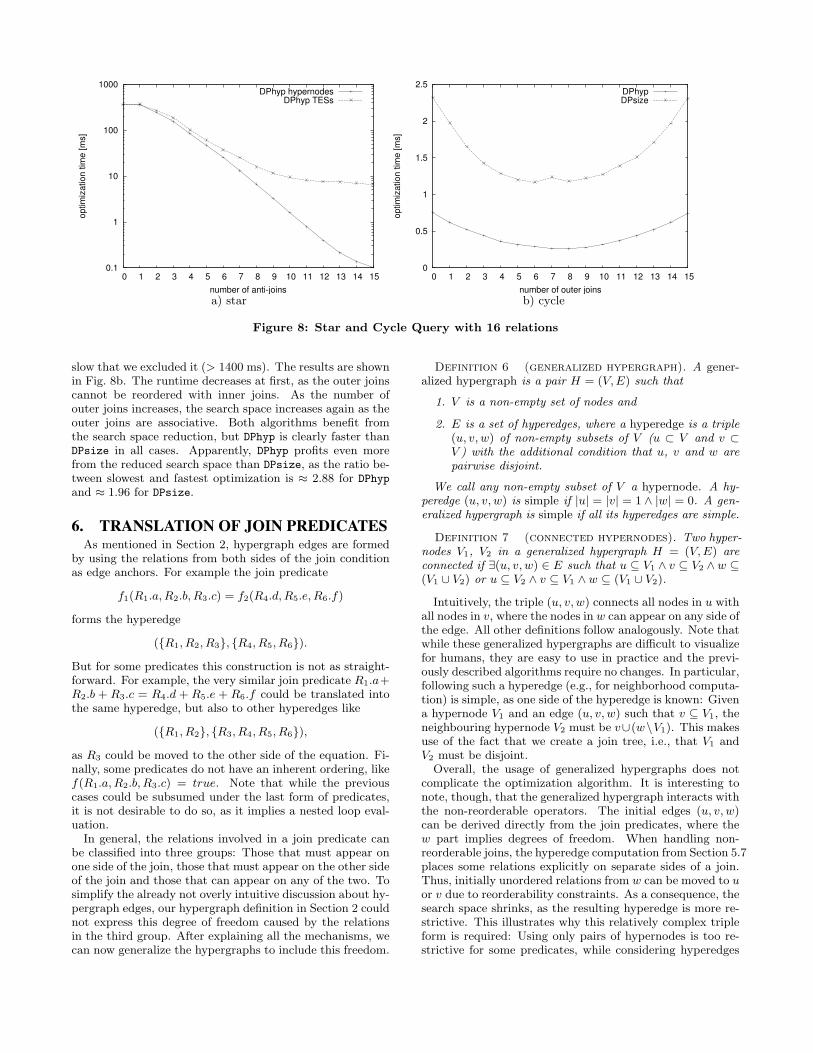
In the first experiment, we wanted to answer the questionhow much we benefit from the search space reduction inSec. 5.7. We compared a generate-and-test paradigm usingTESs with deriving hypergraphs from TESs. We constructa left-deep operator tree for a star query with 16 relations,with an increasing number of antijoins. Thus, the searchspace size decreases over time, as the antijoins are more re-strictive than inner joins. The results are shown in Fig. 8a.For both approaches the optimization time decreases as thesearch space shrinks, but the hypergraph performs muchbetter. The reason is that a TES-test-based approach gen-erates many plans which have to be discarded, while thehypergraph-based formulation can avoid generating them.This shows that hypergraphs can greatly reduce the opti-mization time when handling non-inner joins, even thoughthe original query does not induce a hypergraph.

Antijoins are very restrictive. Hence, the relevant searchspace shrinks quite fast. Outer joins are more interesting,as they can be reordered relatively to each other, which in-creases the search space again. To study this effect andto get a better comparison with the other algorithms, weconstruct a cycle query with 16 relations similar to the starquery above, and replaced inner joins with outer joins. Notethat cycle queries are very favorable for DPsize. DPsub is so

0.1

1

10

100

1000

0 1 2 3 4 5 6 7 8 9 10 11 12 13 14 15

optim

ization tim

e [m

s]

number of anti-joins

DPhyp hypernodesDPhyp TESs

0

0.5

1

1.5

2

2.5

0 1 2 3 4 5 6 7 8 9 10 11 12 13 14 15

optim

ization tim

e [m

s]

number of outer joins

DPhypDPsize

a) star b) cycle

Figure 8: Star and Cycle Query with 16 relations

slow that we excluded it (> 1400 ms). The results are shownin Fig. 8b. The runtime decreases at first, as the outer joinscannot be reordered with inner joins. As the number ofouter joins increases, the search space increases again as theouter joins are associative. Both algorithms benefit fromthe search space reduction, but DPhyp is clearly faster thanDPsize in all cases. Apparently, DPhyp profits even morefrom the reduced search space than DPsize, as the ratio be-tween slowest and fastest optimization is ≈ 2.88 for DPhyp

and ≈ 1.96 for DPsize.

6. TRANSLATION OF JOIN PREDICATESAs mentioned in Section 2, hypergraph edges are formed

by using the relations from both sides of the join conditionas edge anchors. For example the join predicate

f1(R1.a, R2.b, R3.c) = f2(R4.d, R5.e, R6.f)

forms the hyperedge

({R1, R2, R3}, {R4, R5, R6}).

But for some predicates this construction is not as straight-forward. For example, the very similar join predicate R1.a+R2.b + R3.c = R4.d + R5.e + R6.f could be translated intothe same hyperedge, but also to other hyperedges like

({R1, R2}, {R3, R4, R5, R6}),

as R3 could be moved to the other side of the equation. Fi-nally, some predicates do not have an inherent ordering, likef(R1.a, R2.b, R3.c) = true. Note that while the previouscases could be subsumed under the last form of predicates,it is not desirable to do so, as it implies a nested loop eval-uation.

In general, the relations involved in a join predicate canbe classified into three groups: Those that must appear onone side of the join, those that must appear on the other sideof the join and those that can appear on any of the two. Tosimplify the already not overly intuitive discussion about hy-pergraph edges, our hypergraph definition in Section 2 couldnot express this degree of freedom caused by the relationsin the third group. After explaining all the mechanisms, wecan now generalize the hypergraphs to include this freedom.

Definition 6 (generalized hypergraph). A gener-alized hypergraph is a pair H = (V, E) such that

1. V is a non-empty set of nodes and

2. E is a set of hyperedges, where a hyperedge is a triple(u, v, w) of non-empty subsets of V (u ⊂ V and v ⊂V ) with the additional condition that u, v and w arepairwise disjoint.

We call any non-empty subset of V a hypernode. A hy-peredge (u, v, w) is simple if |u| = |v| = 1 ∧ |w| = 0. A gen-eralized hypergraph is simple if all its hyperedges are simple.

Definition 7 (connected hypernodes). Two hyper-nodes V1, V2 in a generalized hypergraph H = (V, E) areconnected if ∃(u, v, w) ∈ E such that u ⊆ V1 ∧ v ⊆ V2 ∧w ⊆(V1 ∪ V2) or u ⊆ V2 ∧ v ⊆ V1 ∧ w ⊆ (V1 ∪ V2).

Intuitively, the triple (u, v, w) connects all nodes in u withall nodes in v, where the nodes in w can appear on any side ofthe edge. All other definitions follow analogously. Note thatwhile these generalized hypergraphs are difficult to visualizefor humans, they are easy to use in practice and the previ-ously described algorithms require no changes. In particular,following such a hyperedge (e.g., for neighborhood computa-tion) is simple, as one side of the hyperedge is known: Givena hypernode V1 and an edge (u, v, w) such that v ⊆ V1, theneighbouring hypernode V2 must be v∪(w\V1). This makesuse of the fact that we create a join tree, i.e., that V1 andV2 must be disjoint.

Overall, the usage of generalized hypergraphs does notcomplicate the optimization algorithm. It is interesting tonote, though, that the generalized hypergraph interacts withthe non-reorderable operators. The initial edges (u, v, w)can be derived directly from the join predicates, where thew part implies degrees of freedom. When handling non-reorderable joins, the hyperedge computation from Section 5.7places some relations explicitly on separate sides of a join.Thus, initially unordered relations from w can be moved to uor v due to reorderability constraints. As a consequence, thesearch space shrinks, as the resulting hyperedge is more re-strictive. This illustrates why this relatively complex tripleform is required: Using only pairs of hypernodes is too re-strictive for some predicates, while considering hyperedges

as connecting an unordered set of nodes (as is sometimesdone for hypergraphs) is wasteful for the search space. Bycombining them, we can both maintain expressiveness andpreserve an efficient exploration of the search space.

7. RELATED WORKWe already discussed closely related approaches in Sec-

tion 5.3. Hence, we give only a brief overview here. Whilethere exist many algorithms for ordering inner joins (see [16]for an overview), there exist only very few to deal with otherjoin operators and hypergraphs.

The basic idea of using csg-cmp-pairs for join enumerationfor simple graphs was published in [17]. DeHaan and Tompaused the same idea to formulate a top down algorithm [7].In both cases, neither hypergraphs nor operators other thaninner joins have been considered.

Galindo-Legaria and Rosenthal extend DPsize to deal withfull and left outer joins [11]. They extend DPsize by incorpo-rating a conflict analysis, which analyzes paths in the querygraph to detect conflicting join operators. However, the ex-tension to hypergraphs was left to Bhargava et al. [1]. Themain idea here is to analyze paths in a hypergraph to detectpossible conflicts.

A much simpler ordering test using EELs has been pro-posed by Rao et al. [19]. It performs a bottom-up traversalof the initial operator tree and builds relation dependencies,handling left outer joins and antijoins. They extend DPsize

with an EEL test much in the same way as our first (lessefficient) alternative (see Sec. 5.8). A more thorough discus-sion of their approach and the differences to our approachcan be found in Sec. 5.3 and 5.5.

8. CONCLUSIONWe presented DPhyp, a join enumeration algorithm ca-

pable of handling hypergraphs and a much wider class ofjoin operators than previous approaches. The extension tohypergraphs enables us to optimize queries with non-innerjoins much more efficiently than before, even for queries withbinary join predicates.

Although our algorithm is way the fastest competitor forjoin ordering for complex queries, there is still plenty of roomfor future research. First, the generation of csg-cmp-pairsstill does some generate-and-test. It will be interesting to seewhether connected subgraphs of hypergraphs can be gener-ated without any tests. Further, compensation is a meansto allow for more reordering if there is a conflict [1, 11, 19].Our algorithm does not incorporate compensation. Thus,this is a natural next step to consider. Lately, a new ap-proach for a top-down join enumeration algorithm has beenproposed by DeHaan and Tompa [7]. It is only a linear fac-tor apart from the optimal solution and thus highly superiorto existing top-down join enumeration algorithms. It suffersfrom the same issues as DPccp did, namely, no hypergraphand no outer join support. It will be interesting to see howtheir algorithm can be extended to deal with these issues.

Acknowledgement. We thank Guy Lohman for point-ing out the importance of hypergraphs, Simone Seeger forher help preparing the manuscript, and Vasilis Vassalos andthe anonymous referees for their help to improve the read-ability of the paper.

9. REPEATABILITY ASSESSMENT RESULTAll the results in this paper were verified by the SIGMOD

repeatability committee.

10. REFERENCES[1] G. Bhargava, P. Goel, and B. Iyer. Hypergraph based

reorderings of outer join queries with complexpredicates. In SIGMOD, pages 304–315, 1995.

[2] G. Bhargava, P. Goel, and B. Iyer. Simplification ofouter joins. In CASCOM, 1995.

[3] S. Bitzer. Design and implementation of a queryunnesting module in Natix. Master’s thesis, U. ofMannheim, 2007.

[4] M. Brantner, S. Helmer, C.-C. Kanne, andG. Moerkotte. Full-fledged algebraic XPath processingin Natix. In ICDE, pages 705–716, 2005.

[5] D. Chatziantoniou, M. Akinde, T. Johnson, andS. Kim. The MD-Join: An Operator for ComplexOLAP. In ICDE, pages 524–533, 2001.

[6] S. Cluet and G. Moerkotte. Classification andoptimization of nested queries in object bases.Technical Report 95-6, RWTH Aachen, 1995.

[7] D. DeHaan and F. Tompa. Optimal top-down joinenumeration. In SIGMOD, pages 785–796, 2007.

[8] C. Galindo-Legaria. Outerjoin Simplification andReordering for Query Optimization. PhD thesis,Harvard University, 1992.

[9] C. Galindo-Legaria and M. Joshi. Orthogonaloptimization of subqueries and aggregation. InSIGMOD, pages 571–581, 2001.

[10] C. Galindo-Legaria and A. Rosenthal. How to extenda conventional optimizer to handle one- and two-sidedouterjoin. In ICDE, pages 402–409, 1992.

[11] C. Galindo-Legaria and A. Rosenthal. Outerjoinsimplification and reordering for query optimization.TODS, 22(1):43–73, Marc 1997.

[12] P. Gassner, G. Lohman, and K. Schiefer. Queryoptimization in the IBM DB2 family. IEEE DataEngineering Bulletin, 16:4–18, Dec. 1993.

[13] E. Kogan, G. Schaller, M. Rys, H. Huu, andB. Krishnaswarmy. Optimizing runtime XMLprocessing in relational databases. In XSym, pages222–236, 2005.

[14] N. May, S. Helmer, and G. Moerkotte. Strategies forquery unnesting in XML databases. TODS,31(3):968–1013, 2006.

[15] N. May and G. Moerkotte. Main memoryimplementations for binary grouping. In XSym, pages162–176, 2005.

[16] G. Moerkotte. Building query compilers. available atdb.informatik.uni-mannheim.de/moerkotte.html.en,2006.

[17] G. Moerkotte and T. Neumann. Analysis of twoexisting and one new dynamic programming algorithmfor the generation of optimal bushy trees without crossproducts. In VLDB, pages 930–941, 2006.

[18] S. Pal, I. Cseri, O. Seeliger, M. Rys, G. Schaller,W. Yu, D. Tomic, A. Baras, B. Berg, and E. K.D. Churin. Xquery implementation in a relationaldatabase system. In VLDB, pages 1175–1186, 2005.

[19] J. Rao, B. Lindsay, G. Lohman, H. Pirahesh, and

D. Simmen. Using EELs: A practical approach toouterjoin and antijoin reordering. In ICDE, pages595–606, 2001. IBM Tech. Rep. RJ 10203.

[20] A. Rosenthal and C. Galindo-Legaria. Query graphs,implementing trees, and freely-reorderable outerjoins.In SIGMOD, pages 291–299, 1990.

[21] P. Selinger, M. Astrahan, D. Chamberlin, R. Lorie,and T. Price. Access path selection in a relationaldatabase management system. In SIGMOD, pages23–34, 1979.

[22] H. Steenhagen. Optimization of Object QueryLanguages. PhD thesis, University of Twente, 1995.

[23] J. Ullman. Database and Knowledge Base Systems,volume Volume 2. Computer Science Press, 1989.

[24] B. Vance and D. Maier. Rapid bushy join-orderoptimization with cartesian products. In SIGMOD,pages 35–46, 1996.

APPENDIXA. EQUIVALENCES AND CONFLICT RULES

In Section 5.5 we needed conflcit rules for all consideredoperators. The following two subsections provide an overviewover all equivalences and conflict rules. The first subsectiondeals with operators nested on the left side, the second withoperators nested on the right side. Note that this is re-dundant, but it is better for an overview of the situation.There is a parenthesized comment on every equivalence orconflict rules. Within these comments, you sometimes findpST (pRS) strong. This has to be read as pST (pRS) strongwith respect to S. Further, the numbers 4.?? refer to equiv-alences in Galindo-Legarias thesis [8].

A.1 Equivalences and Conflict Rules for LeftNesting

Let R, S, and T be arbitrary algebraic expression in ouroperators. Then, assume that we have an expression E

(R ◦p1 S) ◦p2 T

and would like to reorder it to E′, which looks as follows:

R ◦p1 (S ◦p2 T )

For our original expression E, we observe the following:

FT (T ) ⊆ T (R) ∪ T (S)

FT (S) ⊆ T (R)

FT (p1) ⊆ T (R) ∪ T (S)

FT (p2) ⊆ T (R) ∪ T (S) ∪ T (R)

FT (p1) ∩ T (T ) = ∅

These are syntactic constraints, that must be covered.If

FT (p2) ∩ T (R) 6= ∅ ∧ FT (p2) ∩ T (S) 6= ∅

then reodering E to E′ is not possible. However, this is alsocovered by our syntactic constraints SES.

If

FT (p2) ∩ T (R) = ∅ ∧ FT (p2) ∩ T (S) = ∅

then p2 can be a constant predicate like true or false. Thefirst case can lead to e.g. cross products. In the second case,

simplifications apply. If neither is the case, then the predi-cate might reference attributes outside the arguments. Thiskind of algebraic expression results from some nested queries[6]. Anyway, in this paper we do not consider the case thatFT (p2) has no intersection with any argument relations.

Hence, we have to consider only two cases here:

L1 FT (p2) ∩ T (R) 6= ∅ ∧ FT (p2) ∩ T (S) = ∅L2 FT (p2) ∩ T (R) = ∅ ∧ FT (p2) ∩ T (S) 6= ∅Case L1 allows for free reorderability, if no full outerjoin ispresent (see Theorem 1). We will consider Case L2 below.

For commutative operators (B , M), Case L1 can be re-cast to Case L2 by normalzing the operator tree (prior tocalculating SES and T ES) by demanding that

FT (p2) ∩ T (S) 6= ∅

for all commutative operators ◦p1 , which occur on the leftunder some other operator. After this step, all possible con-flicts are of Case L2.

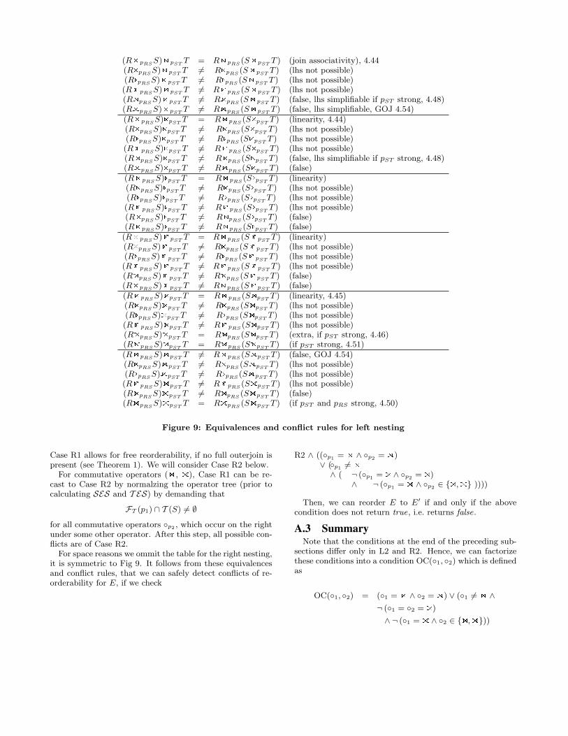
Fig. 9 contains a complete listing of valid and invalid casesfor reordering E to E′. It follows from these equivalencesand conflict rules, that we can safely detect conflicts of re-orderability for E, if we check

L2 ∧ ((◦p1 = B ∧ ◦p2 = M)∨ (◦p1 6= B

∧ ( ¬ (◦p1 = P ∧ ◦p2 = P)∧ ¬ (◦p1 = M ∧ ◦p2 ∈ {P,M} ))))

Then, we can reorder E to E′ if and only if the above con-dition does not return true, i.e. returns false.

A.2 Equivalences and Conflict Rules for RightNesting

Let R, S, and T be arbitrary algebraic expression in ouroperators. Then, assume that we have an expression E

R ◦p1 (S ◦p2 T )

and would like to reorder it to E′, which is defined as follows:

(R ◦p1 S) ◦p2 T

For our original expression E, we observe the following:

FT (S) ⊆ T (R)

FT (T ) ⊆ T (R) ∪ T (S)

FT (p1) ⊆ T (R) ∪ T (S) ∪ T (R)

FT (p2) ⊆ T (S) ∪ T (R)

FT (p2) ∩ T (R) = ∅

These are syntactic constraints, that must be covered. If

FT (p1) ∩ T (S) 6= ∅ ∧ FT (p1) ∩ T (T ) 6= ∅

then reodering E to E′ is not possible. However, this is alsocovered by our syntactic constraints SES. Again, we do notconsider the case where

FT (p2) ∩ T (R) = ∅ ∧ FT (p2) ∩ T (S) = ∅

here.Hence, we have to consider only two cases here:

R1 FT (p1) ∩ T (S) = ∅ ∧ FT (p1) ∩ T (T ) 6= ∅R2 FT (p1) ∩ T (S) 6= ∅ ∧ FT (p1) ∩ T (T ) = ∅

(RB pRS S)B pST T = RB pRS (S B pST T ) (join associativity), 4.44(RGpRS S)B pST T 6= RGpRS (S B pST T ) (lhs not possible)(RIpRS S)B pST T 6= RIpRS (S B pST T ) (lhs not possible)(RT pRS S)B pST T 6= RT pRS (S B pST T ) (lhs not possible)(RPpRS S)B pST T 6= RPpRS (S B pST T ) (false, lhs simplifiable if pST strong, 4.48)(RMpRS S)B pST T 6= RMpRS (S B pST T ) (false, lhs simplifiable, GOJ 4.54)(RB pRS S)GpST T = RB pRS (SGpST T ) (linearity, 4.44)(RGpRS S)GpST T 6= RGpRS (SGpST T ) (lhs not possible)(RIpRS S)GpST T 6= RIpRS (SGpST T ) (lhs not possible)(RT pRS S)GpST T 6= RT pRS (SGpST T ) (lhs not possible)(RPpRS S)GpST T 6= RPpRS (SGpST T ) (false, lhs simplifiable if pST strong, 4.48)(RMpRS S)GpST T 6= RMpRS (SGpST T ) (false)(RB pRS S)IpST T = RB pRS (SIpST T ) (linearity)(RGpRS S)IpST T 6= RGpRS (SIpST T ) (lhs not possible)(RIpRS S)IpST T 6= RIpRS (SIpST T ) (lhs not possible)(RT pRS S)IpST T 6= RT pRS (SIpST T ) (lhs not possible)(RPpRS S)IpST T 6= RPpRS (SIpST T ) (false)(RMpRS S)IpST T 6= RMpRS (SIpST T ) (false)

(RB pRS S)T pST T = RB pRS (S T pST T ) (linearity)(RGpRS S)T pST T 6= RGpRS (S T pST T ) (lhs not possible)(RIpRS S)T pST T 6= RIpRS (S T pST T ) (lhs not possible)(RT pRS S)T pST T 6= RT pRS (S T pST T ) (lhs not possible)(RPpRS S)T pST T 6= RPpRS (S T pST T ) (false)(RMpRS S)T pST T 6= RMpRS (S T pST T ) (false)(RB pRS S)PpST T = RB pRS (SPpST T ) (linearity, 4.45)(RGpRS S)PpST T 6= RGpRS (SPpST T ) (lhs not possible)(RIpRS S)PpST T 6= RIpRS (SPpST T ) (lhs not possible)(RT pRS S)PpST T 6= RT pRS (SPpST T ) (lhs not possible)(RPpRS S)PpST T = RPpRS (SPpST T ) (extra, if pST strong, 4.46)(RMpRS S)PpST T = RMpRS (SPpST T ) (if pST strong, 4.51)(RB pRS S)MpST T 6= RB pRS (SMpST T ) (false, GOJ 4.54)(RGpRS S)MpST T 6= RGpRS (SMpST T ) (lhs not possible)(RIpRS S)MpST T 6= RIpRS (SMpST T ) (lhs not possible)(RT pRS S)MpST T 6= RT pRS (SMpST T ) (lhs not possible)(RPpRS S)MpST T 6= RPpRS (SMpST T ) (false)(RMpRS S)MpST T = RMpRS (SMpST T ) (if pST and pRS strong, 4.50)

Figure 9: Equivalences and conflict rules for left nesting

Case R1 allows for free reorderability, if no full outerjoin ispresent (see Theorem 1). We will consider Case R2 below.

For commutative operators (B , M), Case R1 can be re-cast to Case R2 by normalzing the operator tree (prior tocalculating SES and T ES) by demanding that

FT (p1) ∩ T (S) 6= ∅

for all commutative operators ◦p2 , which occur on the rightunder some other operator. After this step, all possible con-flicts are of Case R2.

For space reasons we ommit the table for the right nesting,it is symmetric to Fig 9. It follows from these equivalencesand conflict rules, that we can safely detect conflicts of re-orderability for E, if we check

R2 ∧ ((◦p1 = B ∧ ◦p2 = M)∨ (◦p1 6= B

∧ ( ¬ (◦p1 = P ∧ ◦p2 = P)∧ ¬ (◦p1 = M ∧ ◦p2 ∈ {P,M} ))))

Then, we can reorder E to E′ if and only if the abovecondition does not return true, i.e. returns false.

A.3 SummaryNote that the conditions at the end of the preceding sub-

sections differ only in L2 and R2. Hence, we can factorizethese conditions into a condition OC(◦1, ◦2) which is definedas

OC(◦1, ◦2) = (◦1 = B ∧ ◦2 = M) ∨ (◦1 6= B ∧¬ (◦1 = ◦2 = P)

∧ ¬ (◦1 = M ∧ ◦2 ∈ {P,M}))