dynamic programming models and algorithms for …castlelab.princeton.edu/html/papers/nascimento...
TRANSCRIPT

Submitted to Management Sciencemanuscript
Dynamic programming models and algorithms for themutual fund cash balance problem
Juliana NascimentoDepartment of Operations Research and Financial Engineering, Princeton University, Princeton, NJ 08540,
Warren PowellDepartment of Operations Research and Financial Engineering, Princeton University, Princeton, NJ 08540,
Fund managers have to decide the amount of a fund’s assets that should be kept in cash, considering the
tradeoff between being able to meet shareholder redemptions and minimizing the opportunity cost from
lost investment opportunities. In addition, they have to consider redemptions by individuals as well as
institutional investors, the current performance of the stock market and interest rates, and the pattern of
investments and redemptions which are correlated with market performance. We formulate the problem as
a dynamic program, but this encounters the classic curse of dimensionality. To overcome this problem, we
propose a provably convergent approximate dynamic programming algorithm. We also adapt the algorithm
to an online environment, requiring no knowledge of the probability distributions for rates of return and
interest rates. We use actual data for market performance and interest rates, and demonstrate the quality
of the solution (compared to the optimal) for the top 10 mutual funds in each of nine fund categories. We
show that our results closely match the optimal solution (in considerably less time), and outperform two
static (newsvendor) models. The result is a simple policy that describes when money should be moved into
and out of cash based on market performance.
Key words : Mutual fund cash balance, approximate dynamic programming
History :
1. Introduction
Mutual fund managers have to determine how much cash to keep on hand, striking a balance
between the cost of meeting redemption requests against the opportunity cost of holding cash. The
academic literature typically ignores several dimensions of the problem, such as the characteristics
of the demands for redemptions. For example, the mutual fund has to consider both individual and
institutional investors. Not only are redemption requests by institutional investors much larger,
1

Author: Mutual fund cash balance problem2 Article submitted to Management Science; manuscript no.
they have to be satisfied right away, producing short-term borrowing costs if there is insufficient
cash. The manager has to consider transaction costs and bid-ask spreads. He also has to take into
account whether the market is under or over-performing long-term averages, as well as the pattern
of deposits and redemptions which are correlated with both market performance and interest rates.
In Wermers (2000) and Edelen (1999), the authors present empirical evidence that supports the
value of active fund management, as expenses and transactions costs are considerable factors in
the fund net returns. In particular, these papers point out the significant cost of holding cash in a
mutual fund.
Variations of the cash balance problem have been studied in the academic community in dif-
ferent forms. A survey of deterministic cash balance problems can be found in Srinivasan & Kim
(1986). The deterministic problem assumes demands, market returns and interest rates are known,
but introduces issues such as fixed costs for a transaction, and the modeling of continuous time
processes. A similar deterministic version of this problem is the cash balance problem based on
Sethi & Thompson (1970) and Sethi (1973) and later described in Sethi & Thompson (2000). The
problem is represented by a system of differential equations and the optimal policy is determined
studying the associated Hamiltonian and adjoint functions. Golden et al. (1979) and Jorjani &
Lamar (1994) propose network flow optimization models to deal with efficient management of cash,
investments and short-term loans. Myopic and stationary solutions for a stochastic cash balance
problem are presented in Penttinen (1991).
A related problem is corporate cash holding which is addressed in Kim et al. (2001), Almeida et
al. (2004) and Faulkender & Wang (2006). These papers present a qualitative analysis indicating
that the more volatile the cash flow and the the higher the cost of finance, the more cash holding
is observed. Almeida et al. (2004) also analyzes cash flow sensitivity.
A cash holding problem specifically applied to mutual funds is discussed in Yan (2006). Like
the papers on corporate cash holdings, this paper only deals with qualitative aspects. The author
develops a simplified static model for the problem and then proceeds with a regression analysis
on actual mutual fund data that validates the model predictions. The author only hints, based on
Author: Mutual fund cash balance problemArticle submitted to Management Science; manuscript no. 3
Constantinides (1986), that the holding of cash should be kept within a certain range and it should
be adjusted only when the cash level is too low or too high.
Hinderer & Waldmann (2001) present a broader cash management model which includes a basic
model of the mutual fund cash holding problem as a special case. The authors propose a dynamic
programming formulation but do not address the computational problems that arise as a result of
the curse of dimensionality.
The mutual fund cash holding problem can be viewed as a more complex inventory control
problem (Graves et al. (1981)). The complications arise due to the presence of side variables
not present in a standard inventory context, such as interest rates and market rates of return.
Even inventory problems with one-dimensional state spaces may lead to prohibitive computational
requirements, due to the cardinality of the state space. In the context of a single-item stochastic
lot-sizing problem, Halman et al. (2006) develops approximation algorithms to deal with it.
A related problem in the economic literature is the commodity storage problem (Wright &
Williams (1982, 1984)). This problem assumes an infinite planning horizon where a crop is harvested
each year and a decision regarding the allocation between consumption and changes in inventory
must be taken at each period. Both a dynamic programming analysis and a competitive equilibrium
analysis are discussed in Judd (1998).
We provide a model of the mutual fund cash-management problem that captures several dimen-
sions of a realistic setting. In fact, our model is based on an email sent by an actual fund manager
describing the issues he was facing and could not find the answers in the literature to approach
them. We propose both finite and infinite horizon models. We then describe several methods for
solving these models: a) we give two solutions based on newsvendor models suggested by the mutual
fund manager in his email, b) we give an exact algorithm using backward dynamic programming
(the most detailed version requires three days to solve), and c) we provide an approximate dynamic
programming algorithm. Our ADP algorithm, dubbed the “SPAR-Mutual” algorithm is based on
a procedure described in Powell et al. (2004) which adaptively learns a piecewise linear function
giving the value of cash as a function of market return and interest rates. The SPAR-Mutual

Author: Mutual fund cash balance problem4 Article submitted to Management Science; manuscript no.
algorithm is provably convergent for finite horizon problems (the proof is given in Nascimento &
Powell (2008), based on the proof technique in Nascimento & Powell (to appear)) which uses a
pure exploitation strategy. The algorithm can be used in a model-based implementation (where we
assume that we know the distribution of market returns and interest rates) over a finite horizon,
or a model-free implementation if we are willing to assume steady state, using actual (rather than
simulated) observations of the exogenous information.
2. Problem Description and Assumptions
Our problem is to determine how much cash to keep on hand to strike a balance between having
enough cash to handle redemptions, and maximizing the return on invested assets. We consider
both finite and infinite horizon versions of this problem. The objective is to minimize discounted
expected costs, where costs include early liquidation costs (if we have to liquidate assets to meet a
redemption request), borrowing costs (if a redemption request has to be satisfied before assets can
be liquidated), transaction costs and the lost return on funds that are not invested in the market.
During periods of market decline, the lost return is negative. We disregard the use of cash to pay
management fees and other expenses and to make dividends and capital gains distributions, since
they are typically a fixed percentage of the total assets under consideration.
There are two types of shareholders, namely large institutional investors and small retail cus-
tomers. We denote by Dlt and Ds
t the demand for redemption at time t from institutional (large)
and retail (small) investors, respectively. We denote by Dit the inflow of money from new investors,
treated as a single, aggregate quantity. We assume that the stochastic processes describing Dlt, Ds
t
and Dit are Markovian. Moreover, they are integer, bounded and positive.
We denote by Rt the cash level at period t after new deposits Dit have been added. If the total
demand for redemption Dlt +Ds
t at t is larger than Rt, then part of the fund portfolio must be
liquidated in order to meet the demand. The cost involved will be denoted by ρsh, the shortfall
cost, given by a deterministic fraction of the liquidating amount. We note that we can easily
accommodate increasing costs for larger transactions which might arise from the cost of liquidating

Author: Mutual fund cash balance problemArticle submitted to Management Science; manuscript no. 5
illiquid assets. If the institutional demand alone is higher than Rt, then a financial cost (interest
rate), denoted by P ft , is also charged, as the demand must be satisfied immediately through short
term loans while securities are liquidated (a process that can require several days). On the other
hand, if too much cash is maintained, the portfolio is losing investment opportunities. This loss is
measured using the fund’s portfolio rate of return, denoted by P rt . P f
t and P rt are Markov processes
(not necessarily independent) which are exogenous to the system. We also assume they have finite
support. Continuous processes could be discretized appropriately in order to apply the algorithms.
We let Wt = (P rt , P
ft ,D
it,D
lt,D
st ) be the vector of exogenous information that becomes avail-
able at every time period t. We assume that Wt is independent of the cash level. Moreover,
(P rt , P
ft ) is conditionally independent of (Di
t,Dlt,D
st ) given Wt−1, that is, IE
[P rt P
ft D
itD
ltD
st |Wt−1
]=
IE[P rt P
ft |Wt−1
]IE [Di
tDltD
st |Wt−1]. We note that more general structures, other than the Markovian
assumption, could be considered for the processes. As a consequence, we would have to augment
Wt with additional features.
Knowing Wt and Rt, the cash rebalancing decision xt = (xt1, xt2) is made, where xt1 is the amount
of money to transfer from the portfolio to the bank account, while xt2 is the amount of money to
transfer from the bank account to the portfolio. There is a limit on the amount of the portfolio
that can be liquidated in one period, so we impose the constraint 0 ≤ xt1 ≤M , where M is a
deterministic bound. Normally, M would simply be chosen large enough that it never constrains
the optimal solution, but it can also be justified by the 1940 Investment Company Act1 which
allows redemptions to be satisfied using shares of stock instead of cash if a redemption request is
too large.
It is obvious that 0≤ xt2 ≤max(0,Rt−Dlt−Ds
t ). We denote by X (Wt,Rt) the feasible region for
xt = (xt1, xt2). The fund incurs transaction costs ρtr for each dollar moved into or out of the fund,
which means that total transaction costs are given by ρtr(xt1 +xt2). Moreover, we assume that the
shortfall cost ρsh is larger than the transaction cost ρtr. Finally, we assume that IE[P ft |P f
t−1
]is
positive and IE[P rt |P r
t−1
]is greater than −ρsh and −ρtr. Clearly, ρsh and ρtr must be positive.
1 http://www.sec.gov/about/laws.shtml#invcoact1940

Author: Mutual fund cash balance problem6 Article submitted to Management Science; manuscript no.
We denote by Rxt the cash level at the end of period t after the decision is taken. This means
that Rxt =max(0,Rt−Dl
t−Dst ) +xt1−xt2 and Rt+1 =Rx
t +Dit+1. Note that since we assume that
Dlt, Ds
t and Dit are integer and bounded, then Rt, xt1, xt2 and Rx
t are also integer and bounded.
The state of the system before the decision is made is denoted by St = (Wt,Rt), while the state of
the system after the decision is made is denoted by Sxt = (Wt,Rxt ).
The one period cost is given by
Ct(St, xt) = ρsh(Dlt +Ds
t −Rt)1{Dlt+Ds
t≥Rt}+P ft (Dl
t−Rt)1{Dlt≥Rt}
+P rt (Rt−Dl
t−Dst )1{Dl
t+Dst<Rt}+ ρtr(xt1 +xt2).
(1)
The first term is the shortfall cost, while the second term is the financial cost. The third term is
the opportunity cost and the last term is the transaction cost.
Let Xπt (St) be a decision function which determines xt given the information in St. We assume
that we have a family of functions Xπt , π ∈ Π. We consider both stationary and nonstationary
policies in this paper, so for the purpose of properly representing nonstationary policies, the decision
function is indexed by time. When we refer to a policy π, we mean the decision function Xπt for
some policy π ∈Π. Later, we provide more specific meaning to a specific policy.
Our problem is to solve
infπ∈Π
IET∑t=0
γtCt(St,Xπt (St))
where γ is a discount factor between 0 and 1. There are two strategies we can use to solve the
problem (we test both in our experimental work). The first is an offline strategy where we use prior
history to update our forecasts at each time period t, from which we generate what is typically a
nonstationary forecast of the future. For example, we may feel that a sudden drop in the market
will be followed by a fairly fast return to normal levels over the next few days. We would implement
such a strategy using a finite horizon model (T might be five or 10 days).
The second strategy is an online implementation where we assume that all processes are sta-
tionary. In this case, we would use an infinite-horizon objective (T =∞). We demonstrate how
a steady-state model such as this can be implemented very easily, without requiring an explicit
update to short-term forecasts.

Author: Mutual fund cash balance problemArticle submitted to Management Science; manuscript no. 7
3. Mutual Fund Cash Holding Models
We first introduce a dynamic programming model where decisions at time t consider their impact
on the future. This model is compared to two static models which use myopic policies. The first
one is a straightforward simplification of the dynamic model, in the sense that the only difference
between them is that the value function will not play a role when a decision is taken. This way,
we are able to measure the importance of the role of the value function, since it adds significant
computational burden to solve the problem. The second static model, proposed by Yan (2006), is
even simpler. It does not consider transaction costs and there is no distinction between the two
types of demand.
The policy obtained from minimizing the cost is the same as the one obtained from maximizing
the profit. Since the original approximate algorithm deals with profit maximization, we use this
terminology when describing the models and algorithmic strategies.
3.1. The Dynamic Model
We start this section discussing the optimal value functions for the cash holding problem. In section
2, we introduced the state of the system, at time t, before and after the decision is taken, denoted
by St = (Wt,Rt) and Sxt = (Wt,Rxt ), respectively. We let V ∗t (St) be the optimal value of being in
state St, where
V ∗t (St) = maxx∈X (Wt,Rt)
−Ct(Wt,Rt, x) + supπ∈Π
IE
[T∑
t′=t+1
−γt′−tCt′(St′ ,Xπ
t (St′))|(St, x)
].
Similarly, we let V ∗,xt (Sxt ) be the optimal value of being in post-decision state Sxt , where
V ∗,xt (Sxt ) = supπ∈Π
IE
[T∑
t′=t+1
−γt′−tCt′(St′ ,Xπ
t (St′))|Sxt
].
Equivalently, the optimal value functions can be defined recursively. Using the value functions
around the pre- and post-decision states, we break Bellman’s equation into two steps:
V ∗,xt−1(Wt−1,Rxt−1) = IE
[V ∗t (Wt,Rt)|(Wt−1,R
xt−1)
], (2)
V ∗t (Wt,Rt) = maxx∈X (Wt,Rt)
−Ct(Wt,Rt, x) + γV ∗,xt (Wt,Rxt ), (3)

Author: Mutual fund cash balance problem8 Article submitted to Management Science; manuscript no.
At time t= T , since it is the end of the planning horizon, V ∗,xT (WT ,RxT ) = 0. At time t− 1, for t=
T, . . . ,1, the value of being in any post-decision state (Wt−1,Rxt−1) does not involve the solution of
an optimization problem, it only involves an expectation, since the next pre-decision state (Wt,Rt)
only depends on the exogenous information that first becomes available at t, as in (2). On the
other hand, the value of being in any pre-decision state (Wt,Rt) at t does not involve expectations,
since the next post-decision state (Wt,Rxt ) is a deterministic function of Wt, it only requires the
solution of an optimization problem, as in (2).
If we substitute (3) into (2), we get
V ∗,xt−1(Wt−1,Rxt−1) = IE
[max
x∈X (Wt,Rt)−Ct(Wt,Rt, x) + γV ∗,xt (Wt,R
xt )|(Wt−1,R
xt−1)
]. (4)
For algorithmic reasons, throughout the paper, we only use (4), instead of (3) and (2), i.e., we only
consider the value function around the post-decision state. Its main feature is the inversion of the
optimization/expectation order in the value function formula. See Powell (2007), Chapter 4, for a
complete discussion of post-decision states.
In order to simplify notation, we will just drop the superscript x in the value function notation.
We perform a qualitative analysis of (4) in order to provide insights about the optimal policy. This
analysis is also the foundation for the SPAR-Mutual algorithm.
Even without computing the expectation in (4), given the integrality assumptions on Dit, Dl
t
and Dst , the function V ∗t−1(Wt−1, ·) : [0,∞] → IR is piecewise linear with integer break points.
Thus, disregarding its value at (Wt−1,0), the function can be identified uniquely by its slopes{v∗t−1(Wt−1,1), v∗t−1(Wt−1,2), . . . , v∗t−1(Wt−1,Bt−1)
}, where Bt−1 is the upper bound on the cash
level Rxt−1 and v∗t−1(Wt−1,R
xt−1) = V ∗t−1(Wt−1,R
xt−1)−V ∗t−1(Wt−1,R
xt−1− 1).
Assuming the slopes are monotone decreasing in the cash level dimension, that is,
vt(Wt,Rxt )≥ vt(Wt,R
xt + 1), (5)
for all states (Wt,Rxt ), we give a simple and intuitive proof that the optimal cash holding
policy only rebalances the cash holdings when the cash level goes outside a certain range.

Author: Mutual fund cash balance problemArticle submitted to Management Science; manuscript no. 9
To describe the policy, we define the following ranges: R1(Wt) = {R : γvt(Wt,R) > ρtr},
R2(Wt) = {R :−ρtr ≤ γvt(Wt,R)≤ ρtr} and R3(Wt) = {R : γvt(Wt,R)<−ρtr}.
Theorem 1. Given a pre-decision state (Wt,Rxt ), assume (5) for all possible cash levels. Regions
R1(Wt), R2(Wt) and R3(Wt) determine a decision rule for the optimization problem
maxxt∈X (Wt,Rt)
−Ct(Wt,Rt, xt) + γVt(Wt, R+xt1−xt2), (6)
where R= max(0,Rt−Dlt−Ds
t ) and Vt(Wt,R) =R∑r=1
vt(Wt, r). The optimal policy is:
Rule 1: If R ∈R1(Wt): x∗t1 = min(M,max
{xt1 : R+xt1 ∈R1(Wt)
}), x∗t2 = 0;
Rule 2: If R ∈R2(Wt): x∗t1 = 0, x∗t2 = 0;
Rule 3: If R ∈R3(Wt): x∗t1 = 0, x∗t2 = max(R,min
{xt2 : R−xt2 ∈R2(Wt)
}).
Proof: Proof of theorem 1. For any pre-decision state (Wt,Rt), the optimal decision x∗t for (6)
is the same as the optimal decision x∗t of the following linear problem:
maxxt,y,z
− ρtr(xt1 +xt2) + γM∑i=1
vt(Wt, R+ i)yi + γR∑j=1
vt(Wt, R− j)(1− zj)
subject toM∑i=1
yi = xt1
R∑j=1
zj = xt2 0≤ y≤ 1 0≤ z ≤ 1.
Note that even without imposing integrality, each component of y and z is either equal to 0 or
1. Each yi = 1, for i = 1, . . . ,M , represents the decision to transfer one dollar from the portfolio
to the bank account. On the other hand, each zj = 1, for j = 1, . . . , R represents the transfer of
one dollar from the bank account to the portfolio. Moreover, given (5), if for some i, y∗i = 1 then
y∗i′ = 1 for all i′ < i, y∗i′′ = 0 for all i′′ > i and the entire vector z is equal to 0. Furthermore, if
for some j, z∗j = 1 then z∗j′ = 1 for all j′ < j, z∗j′′ = 0 for all j′′ > j and the entire vector y is
equal to 0. This follows the logical reasoning that if money is transferred from the portfolio to
the bank account it makes no sense to transfer money from the bank account to the portfolio.
Clearly, if R ∈R1(Wt), then the optimal vector z∗ is equal to zero and y∗i = 1 for all i such that
γvt(Wt, R+ i)>ρtr, that is, we keep transferring money to the bank account while the transaction
cost is smaller than the marginal value of having one more dollar in cash or until the upper bound
Author: Mutual fund cash balance problem10 Article submitted to Management Science; manuscript no.
M is reached. Symmetrically, if R ∈R3(Wt), then the optimal vector y∗ is equal to zero and z∗j = 1
for all j such that γvt(Wt, R− j)<−ρtr, that is, we keep transferring money to the portfolio while
the transaction cost is smaller than the marginal value of having one less dollar in cash or until
there is no more cash to be transferred. Finally, if R ∈R2(Wt), then y∗ = 0 and z∗ = 0, since the
transaction cost is too high to justify any transfer of money, proving rules 1-3. �
We next give an expression for the optimal slopes and show that they are monotonically decreas-
ing, a property that we exploit in the SPAR-Mutual algorithm. This property not only accelerates
the rate of convergence of the algorithm, but it is also central to its pure exploitation nature,
resulting in a simpler and faster procedure.
Theorem 2. For t= T, . . . ,1 and all states (Wt−1,Rxt−1), the optimal slopes are given by
v∗t−1(Wt−1,Rxt−1) = IE
[G(Wt,Rt, v
∗t )|(Wt−1,R
xt−1)
], (7)
where
G(Wt,Rt, v∗t ) = ρsh1{Dl
t+Dst≥Rt}+P f
t 1{Dlt≥Rt}−P
rt 1{Dl
t+Dst<Rt}
+ max(ρtr, γv∗t (Wt,Rt−Dl
t−Dst +Mt)
)1{γv∗t (Wt,Rt−Dl
t−Dst )>ρtr}1{Dl
t+Dst<Rt}
+ γv∗t (Wt,Rt−Dlt−Ds
t )1{−ρtr≤γv∗t (Wt,Rt−Dlt−D
st )≤ρtr}1{Dl
t+Dst<Rt}
− ρtr1{γv∗t (Wt,Rt−Dlt−D
st )<−ρtr}1{Dl
t+Dst<Rt}.
Moreover, the optimal slopes are monotone decreasing in the cash level dimension, that is,
v∗t−1(Wt−1,Rxt−1)≥ v∗t−1(Wt−1,R
xt−1 + 1),
implying concavity of the optimal value function.
The proof of Theorem 2 is given in the appendix.
3.2. The Static Models
In our first static model, given the time period t and the pre-decision state (Wt,Rt), the objective
is to find a decision that maximizes the expected profit in the next time period, where the profit

Author: Mutual fund cash balance problemArticle submitted to Management Science; manuscript no. 11
is the negative of the cost given by (1). The second model is similar to the one proposed in Yan
(2006). It does not consider transaction costs and there is no distinction between the two types
of demand. Because of the latter simplification, the finance and the shortfall costs are collapsed
together. As in the first static model, given the time period t and the pre-decision state (Wt,Rt),
the objective is to find a decision that maximizes the expected profit in the next time period, where
the expression for the profit takes into consideration the simplifications mentioned above.
Let Dt+1 = Dlt+1 +Ds
t+1 −Dit+1 be the net flow of money. For the first and second model, the
optimal decision x∗t is thus found by solving, respectively, the maximization problems:
maxxt∈X (Wt,Rt)
IE[−Ct+1(Wt+1,R
xt +Di
t+1, xt)|(Wt,Rt)], (8)
maxxt∈X (Wt,Rt)
IE[−(ρsh +P f
t+1)(Dt+1−Rxt )1{Dt+1≥Rx
t }−Prt+1(Rx
t −Dt+1)1{Dt+1<Rxt }|(Wt,Rt)
], (9)
where Rxt = max(0,Rt−Dl
t−Dst ) +xt1−xt2.
4. Algorithmic Strategies
In this section, we present algorithms to actually compute the decisions implied by each cash
holding model. For the dynamic setting, once we compute the slopes of the value functions, a
solution is easily determined following the decision rule described in Theorem 1. We propose two
approaches to find the slopes. The first one is traditional backward dynamic programming. Even
though this approach is simple and straightforward, it is computationally very demanding.
The second approach is through approximate dynamic programming (ADP). The ADP algorithm
replaces the computation of the expected value by iteratively observing sample path realizations
and, most importantly, by exploiting the structural property of the optimal slopes, namely the
monotone decreasing property. Of course, ADP replaces the computational burden of the exact
solution with the statistical errors of a Monte-Carlo based procedure. The upside is that the
slopes do converge to the optimal ones in the limit. The idea is that if the number of iterations is
large enough, the approximate solutions are very close to the optimal ones. The ADP approach is
discussed in full in the next section.

Author: Mutual fund cash balance problem12 Article submitted to Management Science; manuscript no.
The optimal decision for the static models is obtained in a similar fashion as the optimal decision
for the dynamic model at time period T−1, since no downstream effects are taken into consideration
at the end of the planning horizon T . Therefore, our procedure to determine the optimal decision
for the static models follows the reasoning of the proof of Theorem 1, i.e., we make the decision
comparing the transaction cost with the marginal value of transferring one dollar to/from the bank
account.
Given the pre-decision state (Wt,Rt), let f1(Wt,Rxt ) and f2(Wt,R
xt ) denote the marginal value
of transferring one dollar to the bank account for the first and second static models, respectively,
when the cash level is Rxt = max(0,Rt−Dl
t−Dst )+xt1−xt2. From (8) and (9), we can easily obtain
f1(Wt,Rxt ) =Ef IP{Dl
t+1−Dit+1 ≥Rx
t |(Wt,Rt)}+ (ρsh +Er)IP{Dt+1 ≥Rxt |(Wt,Rt)}−Er,
f2(Wt,Rxt ) = (Ef + ρsh +Er)IP{Dt+1 ≥Rx
t |(Wt,Rt)}−Er,
where Ef = IE[P ft+1|Wt], Er = IE[P r
t+1|Wt] and Dt+1 = Dlt+1 + Ds
t+1 − Dit+1. Symmetrically, the
marginal value of transferring one dollar from the bank account is given by −f1(Wt,Rxt ) and
−f2(Wt,Rxt ), respectively.
The optimal decision for the first model can be found using the procedure:
STEP 0: Initialize xt1 = xt2 = 0.
STEP 1: While f1(Wt,Rxt )>ρtr and xt1 <Mt do xt1 = xt1 + 1.
STEP 2: While f1(Wt,Rxt )<−ρtr and xt2 <max(0,Rt−Dl
t−Dst ) do xt2 = xt2 + 1.
Since there is no transaction cost involved in the second model, its solution is determined using a
similar procedure, replacing ρtr by zero and f1(Wt,Rxt ) by f2(Wt,R
xt ).
5. The Approximate Dynamic Programming Approach
The main idea of the algorithm is to construct concave and piecewise linear function approximations
V nt (Wt, ·), learning its slopes vnt (Wt,R
xt1), . . . , vnt (Wt,R
xtN) over the iterations. At each iteration, our
decision function looks like
Xπt (Snt ) = arg max
xt∈X (Wnt ,R
nt )
−Ct(Snt , xt) + γV n−1t (W n
t ,Rxt )

Author: Mutual fund cash balance problemArticle submitted to Management Science; manuscript no. 13
where V n−1t (Wt, ·) is the piecewise, linear value function approximation computed using information
up through iteration n−1. We now see that our policy is parameterized by the slopes vn−1t (Wt, r),
r= 1,2, . . . for each possible value of Wt. Thus, when we refer to a policy π, we are actually referring
to a specific set of slopes.
The catch is that the algorithm does not try to learn the slopes for the whole state space, only for
parts close to optimal cash levels, which are determined by the algorithm itself. Figure 1 illustrates
the idea.
������������������������������������������������������������������������������������������������������������������������������������������������������������������������������������������������������������������������������������������������������������������������������������������������������������������������������������������������������������������������������������������������������������������������������������������������������������������������������������������������������������������������������������������������������������������������������������������������������������������������������������������������������
������������������������������������������������������������������������������������������������������������������������������������������������������������������������������������������������������������������������������������������������������������������������������������������������������������������������������������������������������������������������������������������������������������������������������������������������������������������������������������������������������������������������������������������������������������������������������������������������������������������������������������������������������
Important Region
Asset Dimension
V ∗t (Wt, ·) V nt (Wt, ·)
Approximation - Constructed
Rxt1 Rx
t2 Rxt3
v nt (W
t ,R xt5 )
v ∗t (W
t ,R xt4 )
v∗t(Wt,Rxt3)
v∗t(W t,R
xt2)
v∗ t(Wt,Rx t1)
Optimal - Unknown
vn t(W
t,Rx t1)
vnt(W
t,Rxt2)
vnt (Wt,Rxt3) v n
t (Wt ,R x
t4 )
v ∗t (Wt ,R
xt5 )
Figure 1 Optimal value function and the constructed approximation
At each iteration n and time t, instead of computing the expectation in (4), the algorithm
observes one sample realization of the information vector. After that, the sample realization and
the current value function approximation are used to take a decision xnt , leading the system to
a post-decision state. Sample information around the new post-decision state is gathered and is
used to update the approximate slopes vn−1t−1 . A projection operation is then performed in case a
violation of the concavity property occurs.
5.1. The SPAR-Mutual Algorithm
Before we present the algorithm, some notation is necessary. A general post-decision state at t is
denoted by Sxt or (Wt,Rxt ). The two of them are used interchangeably. We use Sx,nt to denote the
actual post-decision state visited by the algorithm at iteration n and time t. The same notation
convention holds for the pre-decision states. At iteration n and time t, the actual decision taken by
the algorithm is denoted by xnt , while the value function approximation is denoted by V nt (Wt, ·). The

Author: Mutual fund cash balance problem14 Article submitted to Management Science; manuscript no.
STEP 0: Algorithm initialization:
STEP 0a: Initialize v0t (Wt,R
xt ) for all t and (Wt,R
xt ) monotone decreasing in Rx
t .
STEP 0b: Pick N , the total number of iterations.
STEP 0c: Set n= 1.
STEP 1: Planning horizon initialization: Observe the initial cash level Rx,n−1 .
Do for t= 0, . . . , T :
STEP 2: Sample/Observe P f,nt , P r,n
t , Di,nt , Dl,n
t and Ds,nt .
STEP 3: Compute the pre-decision cash level: Rnt =Rx,n
t−1 +Di,nt .
STEP 4: Slope update procedure:
If t > 0 then
STEP 4a: Observe vnt (Rx,nt−1) and vnt (Rx,n
t−1 + 1).
STEP 4b: For all possible states Sxt−1:
znt−1(Sxt−1) = (1− αnt−1(Sxt−1))vn−1t−1 (Sxt−1) + αnt−1(Sxt−1)vnt (Rx
t−1).
STEP 4c: Perform the projection operation vnt−1 = ΠC,Wnt−1,R
x,nt−1
(znt−1). See (10).
STEP 5: Find the optimal solution xnt of maxx∈X (Wn
t ,Rnt )−Ct(Snt , x) + γV n−1
t (W nt ,R
xt ).
STEP 6: Compute the post-decision cash level: Rx,nt = max(0,Rn
t −Dl,nt −Ds,n
t ) +xnt1−xnt2.
STEP 7: If n<N increase n by one and go to step 1. Else, return vN .
Figure 2 SPAR-Mutual Algorithm
corresponding slopes are denoted by vnt (Wt) = (vnt (Wt,1), . . . , vnt (Wt,Bt)). Clearly, V nt (Wt,R
xt ) =∑Rx
tr=1 v
nt (Wt, r). We refer interchangeably to the value function itself and to its slopes.
The SPAR-Mutual algorithm is presented in figure 2. As described in Step 0, the algorithm
inputs are piecewise linear value function approximations represented by their slopes v0t (Wt,R
xt ).
The initial slopes must be decreasing in the cash level dimension. A slope vector that is equal to
zero for all states and time periods is a valid input. Since we know that v∗T (WT ,RxT ) = 0 for all
states (WT ,RxT ), then we use vnT (WT ,R
xT ) = 0 for all iterations n.
At each iteration n, the algorithm starts by observing the initial cash level, denoted by Rx,n−1 , as

Author: Mutual fund cash balance problemArticle submitted to Management Science; manuscript no. 15
in Step 1. The initial cash level must be a positive integer. After that, the algorithm proceeds over
time periods t= 0, . . . , T . At the beginning of time period t, the algorithm generates a sample of
the interest rate P f,nt , rate of return P r,n
t , money inflow Di,nt , institutional redemption Dl,n
t and
retail redemption Ds,nt , as in Step 2. These are Monte Carlo samples following the probability
distribution of the information process Wt given that W nt−1 = (P f,n
t−1, Pr,nt−1,D
i,nt−1,D
l,nt−1,D
s,nt−1). After
that, the pre-decision cash level Rnt is computed, as in Step 3.
Before the decision at time period t is taken, the algorithm uses the sample information to
update the slopes of time period t− 1. Steps 4a-4c describes the procedure and figure 3 illustrates
it. We first observe slopes relative to the post-decision states (W nt−1,R
x,nt−1) and (W n
t−1,Rx,nt−1 + 1)
(see Step 4a and figure 3.a). Then, these sample slopes are used to update the approximation
slopes vn−1t−1 through a temporary slope vector znt−1 (see Step 4b and figure 3.b). This step requires
the use of a stepsize rule that is state dependent, denoted by αnt (Sxt ). We have that αnt (Sxt ) =
αnt 1{Wt=Wnt }(1{Rx
t =Rx,nt }+ 1{Rx
t =Rx,nt +1}), where 0<αnt ≤ 1 and αnt can depend only on information
that became available up through iteration n and time t. For example, it is valid to use αnt = 1N(S
x,nt )
,
where N(Sx,nt ) is the number of visits to state Sx,nt up until iteration n. The updating scheme
may produce slopes that violate the property of being monotonically decreasing. In this case, a
projection operation is performed to restore the property and obtain the updated approximation
slopes vnt−1 (see Step 4c and figure 3.c).
Next, a decision xnt is made given the current state at time t. This decision is the optimal
solution with respect to the current pre-decision state (W nt ,R
nt ) and value function approximation
V n−1t (W n
t , ·), as stated in Step 5. This decision can be easily calculated following the decision rule
described in Theorem 1. We just need to consider the current pre-decision state (W nt ,R
nt ) and the
current slope approximation vn−1t (W n
t ).
Finally, the post-decision state Rx,nt is computed, as in Step 6, and we advance the clock to time
t+ 1. As the algorithm reaches the planning horizon t = T , if the number of iterations has not
reached its limit N , then the iteration counter is incremented, as in Step 7, and a new iteration is

Author: Mutual fund cash balance problem16 Article submitted to Management Science; manuscript no.
FW
n t,R
n t−1,V
n−
1t
(x)
Exact
ATxnt
xRn
t
vnt+1+v
nt+1−
Rnt−1
��������������������������������������������������������������������������������
������������������������������������������������
���������������������������������������
���������������������������������������
������������������������������������
������������������������������������
���������������������������������������������
���������������������������
������
������
���������������������������
���������������������������
Slopes of V n−1t (W n
t )
vn−1t (W n
t ,Rnt )
3.a: Current approximate function, optimal decision and sampled slopes
Concavity violationExact
��������������������������������������������������������������������������������
������������������������������������������������
���������������������������������������
���������������������������������������
����������������������������������������������������������������������
������������������������������������������
������������������������
������������������������
������������������
���������
������������������
������������������
Slopes of znt (W n
t )
znt (W nt ,R
nt )
3.b: Temporary approximate function with violation of concavity
Fr
n t,P
n t,R
n t−1,V
n t(x,y
n t)
Exact
x������������������������
������������������������
���������������������������
���������������������������
������������������
������������������
��������������������������������������������������������������������������������
������������������������������������������������
����������������������������
��������������
���������������������������������������
��������������������������������������� � � � � ����������
Slopes of V nt (W n
t )
vnt (W nt ,R
nt )
3.c: Level projection operation: updated approximate function with concavity restoredFigure 3 Slopes update procedure, where Ft−1(Sn
t−1, Vn−1
t−1 , x) =−Ct−1(Snt−1, x) + γV n−1
t−1 (Wnt−1,R
xt−1).
started from Step 1. Otherwise, the algorithm is finished returning the current slope approximation
vNt (Wt,Rxt ) for all t and (Wt,R
xt ).
We obtain sample slopes by replacing the expectation and the optimal slope v∗t in (7) by the
sample realization W nt and the current slope approximation vn−1
t , respectively. Thus, for t= 1 . . . , T ,
the sample slope is vnt (R) = G(W nt ,R, v
n−1t ).
The projection operator ΠC,Wnt ,R
x,nt
maps a vector znt that may not be monotone decreasing in

Author: Mutual fund cash balance problemArticle submitted to Management Science; manuscript no. 17
the cash level dimension, into another vector vnt that has this structural property. The operator
imposes the property by forcing the newly updated slope at (W nt ,R
x,nt ) to be greater than or equal
to the newly updated slope at (W nt ,R
x,nt + 1) and then forcing the other violating slopes to be
equal to the newly updated ones. For any state (Wt,Rxt ), the projection is given by
ΠC,Wnt ,R
x,nt
(z)(Wt,Rxt ) =
z(Wn
t ,Rx,nt )+z(Wn
t ,Rx,nt +1)
2, if C1
ΠC,Wnt ,R
x,nt
(z)(W nt ,R
x,nt ), if C2
ΠC,Wnt ,R
x,nt
(z)(W nt ,R
x,nt + 1), if C3
z(Wt,Rxt ), otherwise,
(10)
where the conditions C1, C2 and C3 are
C1: Wt =W nt , Rx
t = (Rx,nt or Rx,n
t + 1), z(W nt ,R
x,nt )< z(W n
t ,Rx,nt + 1);
C2: Wt =W nt , Rx
t <Rx,nt , z(Wt,R
xt )≤ΠC,Wn
t ,Rx,nt
(z)(W nt ,R
x,nt );
C3: Wt =W nt , Rx
t >Rx,nt + 1, z(Wt,R
xt )≥ΠC,Wn
t ,Rx,nt
(z)(W nt ,R
x,nt + 1).
5.2. Convergence Analysis
We state two theorems that prove that the algorithm converges to an optimal policy, that is, the
algorithm does learn the optimal decision to be taken at each state that can possibly be reached
by an optimal policy. The proofs are based on more general results in Nascimento et al. (2007),
hence only a sketch is provided here.
We start with some remarks. We denote by {Snt }n≥0 = {(W nt ,R
nt )}n≥0 the sequence of pre-
decision states visited by the algorithm at time t. Likewise, we denote by {xnt }n≥0 the sequence
of decisions taken by the algorithm and by {Sx,nt }n≥0 = {(W nt ,R
x,nt )}n≥0 the sequence of post-
decision states visited by the algorithm. Each one of these sequences has at least one accumulation
point. This result derives from the fact that the information process and the cash level have finite
support. Moreover, the decisions are constrained to compact sets. We denote by S∗t , x∗t and Sx,∗t
the respective accumulation points.
We denote by {vnt (Wt)}n≥0 the sequence of slopes generated by the algorithm. Note that there is
one such sequence for each vector Wt. This sequence also has at least one accumulation point, since
the projection operation guarantees, for all n, that vnt (Wt) belongs to a compact set, namely, the
Author: Mutual fund cash balance problem18 Article submitted to Management Science; manuscript no.
set of vectors that are monotone decreasing in the cash level dimension and are bounded (due to
the finite support assumption of the information process). We denote by v∗t (Wt) an accumulation
point of this sequence.
Theorem 3. On the event that (W ∗t ,R
x,∗t ) is an accumulation point of {(W n
t ,Rx,nt )}n≥0, if
∞∑n=0
αnt (W ∗t ,R
x,∗t ) =∞ and
∞∑n=0
(αnt (W ∗t ,R
x,∗t ))2
<B <∞ a.s.,
then
vnt (W ∗t ,R
x,∗t )→ v∗t (W
∗t ,R
x,∗t ) and vnt (W ∗
t ,Rx,∗t + 1)→ v∗t (W
∗t ,R
x,∗t + 1) a.s. (11)
As a byproduct of the previous theorem, we obtain the next theorem:
Theorem 4. For t = 0, . . . , T , on the event that (W ∗t ,R
∗t , v∗t , x∗t ) is an accumulation of
{(W nt ,R
nt , v
n−1t , xnt )}n≥1, if the stepsize condition of Theorem 3 is satisfied, then, with probability
one, x∗t is an optimal solution of maxxt∈X (W∗t ,R
∗t )Ft(W ∗
t ,R∗t , V
∗t , xt), where
Ft(W ∗t ,R
∗t , V
∗t , xt) =−Ct(W ∗
t ,R∗t , xt) + γV ∗t (W ∗
t ,max(0,R∗t −Dl,∗t −Ds,∗
t ) +xt1−xt2). (12)
Equation (12) implies that the algorithm has learned an optimal decision for all states that can
be reached by an optimal policy. This implication can be easily justified as follows. We start with
t= 0. For each accumulation point (W ∗0 ,R
∗0) of {(W n
0 ,Rn0 )}n≥0, (12) tells us that the accumulation
points x∗0 of {xn0}n≥0 along the iterations with initial pre-decision state (W ∗0 ,R
∗0) are in fact an
optimal decision for period 0 when the pre-decision state is (W ∗0 ,R
∗0). This implies that all accu-
mulation points Rx,∗0 = max(0,R∗0 −D
l,∗0 −D
s,∗0 ) + x∗01 − x∗02 of {Rx,n
0 }n≥0 are post-decision cash
levels that can be reached by an optimal policy. When t= 1, for each Rx,∗0 and each accumulation
point W ∗1 of {W n
1 }n≥0, R∗1 = Rx,∗0 + Di,∗
1 is a pre-decision cash level that can be reached by an
optimal policy. Once again, (12) tells us that the accumulation points x∗1 of {xn1}n≥0 along the iter-
ations with (W n1 ,R
n1 ) = (W ∗
1 ,R∗1) are indeed an optimal decision for period 1 when the pre-decision
state is (W ∗1 ,R
∗1). As before, the accumulation points Rx,∗
1 = max(0,R∗1 −Dl,∗1 −D
s,∗1 ) + x∗11 − x∗12
of {Rx,n1 }n≥0 are post-decision cash levels that can be reached by an optimal policy. The same
reasoning can be applied for t= 2, . . . , T .

Author: Mutual fund cash balance problemArticle submitted to Management Science; manuscript no. 19
6. The Infinite Horizon Cash Holding Problem
The infinite horizon problem arises when we believe that the exogenous information processes
(prices, interest rates, deposits and redemptions) are stationary. The only change is that we drop
the indexing by time of all variables. We adjust the algorithms to the infinite horizon case in a fairly
straightforward way. For the static models, we use the procedure described in section 4, dropping
the time index.
The ADP algorithm for the infinite horizon case is similar to the SPAR-Mutual algorithm
described in figure 2, except that we do not loop over the different time periods and again the time
index is dropped. The modified SPAR-Mutual algorithm for the infinite horizon method brings
a nice twist. It can be considered an online algorithm, in the sense that probability distributions
do not need to be known or estimated. For the finite horizon case, the sample realizations for the
interest rate, rate of return, deposits and withdrawals are obtained from a sample generator that
follows a known distribution. On the other hand, actual daily historical values of the interest rate,
rate of return, inflow money and demand for redemption can be used for the infinite horizon case,
without any need to estimate the probability distribution underlying them. Moreover, as new daily
information becomes available, it can be used to update the current slope approximations. We do
not have a proof of convergence for this online algorithm, but we show that the policies produced
by this algorithm outperform the static ones.
7. Numerical Experiments
The purpose of this section is to analyze the behavior of the different algorithmic approaches. We
study the effect of discretization on CPU time and solution quality for the exact and the ADP
algorithms. Moreover, we quantify how much we gain by considering the impact a decision has
on the future, instead of just using a myopic policy. Finally, for the infinite horizon case, we can
observe the behavior of an online algorithm and the errors incurred in constructing probability
distributions and estimating their parameters.
We want to make sure we compare the algorithmic strategies when they are applied to realistic
environments. To achieve this goal, the probability distributions are estimated using real data,

Author: Mutual fund cash balance problem20 Article submitted to Management Science; manuscript no.
including bank prime loan rates, rates of return of top performing funds, total asset values and
redemption rates of a broad range of funds.
We start by describing the instances considered and the data used to construct them. After
that, we discuss implementation details. We then present and analyze the results for the finite and
infinite horizon cases.
7.1. Problem Instances
We start with the interest rate models. The Vasicek and the Cox-Ingersoll-Ross (CIR) processes
are commonly used to model interest rates (Cairns (2004)). The processes are described by
drt = α(µ − rt)dt + σdBt and drt = α(µ − rt)dt + σ√rtdBt, respectively, where rt represents
the interest rate process, Bt is a standard Brownian motion and α, µ and σ are parameters
that must be estimated. We used discrete time versions of these models, capturing the behav-
ior that decisions are made once each day. Thus, we use rt+1 = rt + α(µ− rt)∆t + σ√
∆tZt and
rt+1 = rt+α(µ−rt)∆t+σ√rt∆tZt, respectively, where Zt is normally distributed with mean 0 and
variance 1, and ∆t is the length of a single day (in whatever units we are measuring time).
We applied the maximum likelihood estimation (MLE) method to fit these parameters, using
weekly prime rate historical data (from July, 2001 to June, 2006) from the Federal Reserve Board
website2, as bank prime loan is one of several base rates used by banks to price short-term business
loans.
For the portfolio rate of return, we used the Vasicek process to model the rate of return. We
consider nine different sets of funds. Each set represents a market capitalization category (large,
mid, small cap) and a style (blend, growth, value). Moreover, each set is composed of the 10 best
performing funds in the given category/style over the past three years according to Yahoo Finance3.
We identify each set using the first letter of the corresponding category/style. For example, LB
represents the set of large blend funds.
2 http://www.federalreserve.gov/releases
3 http://finance.yahoo.com/
Author: Mutual fund cash balance problemArticle submitted to Management Science; manuscript no. 21
Daily rates of return (from July, 2001 to June, 2006) for each fund were collected from the
CRSP Mutual Fund Database 4 and were averaged across the ten funds on each style/category.
The resulting daily rates and the MLE method were used to estimate the parameters of the Vasicek
process.
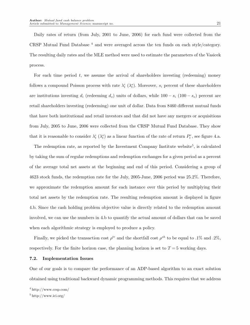
For each time period t, we assume the arrival of shareholders investing (redeeming) money
follows a compound Poisson process with rate λit (λot ). Moreover, si percent of these shareholders
are institutions investing di (redeeming do) units of dollars, while 100− si (100− so) percent are
retail shareholders investing (redeeming) one unit of dollar. Data from 8460 different mutual funds
that have both institutional and retail investors and that did not have any mergers or acquisitions
from July, 2005 to June, 2006 were collected from the CRSP Mutual Fund Database. They show
that it is reasonable to consider λit (λot ) as a linear function of the rate of return P rt , see figure 4.a.
The redemption rate, as reported by the Investment Company Institute website5, is calculated
by taking the sum of regular redemptions and redemption exchanges for a given period as a percent
of the average total net assets at the beginning and end of this period. Considering a group of
4623 stock funds, the redemption rate for the July, 2005-June, 2006 period was 25.2%. Therefore,
we approximate the redemption amount for each instance over this period by multiplying their
total net assets by the redemption rate. The resulting redemption amount is displayed in figure
4.b. Since the cash holding problem objective value is directly related to the redemption amount
involved, we can use the numbers in 4.b to quantify the actual amount of dollars that can be saved
when each algorithmic strategy is employed to produce a policy.
Finally, we picked the transaction cost ρtr and the shortfall cost ρsh to be equal to .1% and .2%,
respectively. For the finite horizon case, the planning horizon is set to T = 5 working days.
7.2. Implementation Issues
One of our goals is to compare the performance of an ADP-based algorithm to an exact solution
obtained using traditional backward dynamic programming methods. This requires that we address
4 http://www.crsp.com/
5 http://www.ici.org/

Author: Mutual fund cash balance problem22 Article submitted to Management Science; manuscript no.
−4 −3 −2 −1 0 1 2 3 4−20
−15
−10
−5
0
5
10
15
Monthly Rate of Return
Mon
thly
Net
Flo
w
Actual DataLinear Regression
LB LG LV MB MG MV SB SG SL0
50
100
150
200
250
300
350
400
450
500
Instance
Red
empt
ion
(in m
illio
ns o
f dol
lars
)
4.a - Average Net Flow 4.b - Approximate redemption amountFigure 4 Net Flow and Redemptions
the fact that the interest rate and rate of return processes are unbounded and continuous, but an
exact solution requires that they be bounded and discrete.
To obtain an exact solution, we had to create a discretized version of the interest rate and return
processes. We did this by first discretizing and truncating the exogenous changes to interest rate
and return processes. Using this modified process, we created a probability distribution for these
processes that reflected both the discretization and the truncation. We then chose the finest level
of discretization that could be solved with reasonable execution times (we allowed run times to
span days), and defined this to be the exact solution. This solution could then be compared to
solutions obtained using backward dynamic programming for coarser levels of aggregation, as well
as solutions obtained using the SPAR-Mutual algorithm.
When using the SPAR-Mutual algorithm, we simulated the original continuous state (that is, the
interest rate and returns – movements of cash were always assumed to occur in discrete quantities).
Sample observations of changes in interest rates and returns were generated by either using the
original continuous distributions or sample observations from history (without discretization). Only
the value function approximation was discretized. This strategy allowed us to estimate the errors
produced using approximate dynamic programming in a realistic setting, but we still compared
our performance against an “exact” model which assumed a very fine level of discretization.

Author: Mutual fund cash balance problemArticle submitted to Management Science; manuscript no. 23
A second important implementation issue was the choice of the right stepsize rule which is a key
ingredient to faster rates of convergence. Even though the stepsize rule αn = 1/N(Sx,nt ) produces
a provably convergent algorithm, the associated rate of convergence is poor, since this rule goes to
zero too quickly. The problem is that while learning the slope for one state, the updating procedure
depends on another slope approximation, which is steadily changing, since the algorithm is also
learning this other slope, leading to a nonstationary process. Moreover, the rate of convergence for
each slope is different and, ideally, the stepsize rule would reflect that. For example, the slower the
convergence of a given slope, the larger its stepsize should be. Since we cannot tune a stepsize rule
for each slope, an adaptive stepsize rule works best. In our implementation, we use the adaptive
stepsize rule proposed in George & Powell (2006). It is given by αnt = 1− (σnt (S
x,nt ))2
δmt (S
x,nt )
, where m is
the number of visits to state Sx,nt up to iteration n. (σnt (Sx,nt ))2 is an estimate of the variance
of the observation error, and δmt (Sx,nt ) is an estimate of the total squared variation between the
observation and the estimate which includes both bias (if our estimates are consistently high or
low) as well as the observation error. These are computed using
δmt (Sx,nt ) = (1− νm−1)δm−1t (Sx,nt ) + νm−1(vnt+1(Rx,n
t )− vn−1t (Sx,nt ))2;
βmt (Sx,nt ) = (1− νm−1)βm−1t (Sx,nt ) + νm−1(vnt+1(Rx,n
t )− vn−1t (Sx,nt ));
(σnt (Sx,nt ))2 =δmt (Sx,nt )− (βmt (Sx,nt ))2
1 + λm−1t (Sx,nt )
.
Here, νm = 10/(10 +m) is a stepsize formula.
The other ingredient to faster rates of convergence is the choice of discretization increments. It is
intuitive to expect that coarser discretization increments (smaller state space) lead to faster rates
of convergence in the initial iterations but poorer results in the long run, while finer discretization
increments (larger state space) lead to slower rates of convergence in the initial iterations but more
accurate results in the long run. The reasoning behind this intuition is that, when the discretization
is fine, in the initial iterations, most of the state space (in the information dimension Wt) does not
have enough observations to produce a reasonable slope approximation. Since the SPAR-Mutual

Author: Mutual fund cash balance problem24 Article submitted to Management Science; manuscript no.
algorithm depends on the slope approximation to make a decision and this decision determines the
further course of the algorithm, the rate of convergence can suffer from this lack of information.
We start the SPAR-Mutual algorithm (for the infinite horizon case) considering a coarse dis-
cretization increment for the rate of return. Then, after N1 iterations, we switch the discretization
increment increasing by a factor of two the state space. We repeat the same procedure after N2
and N3 iterations. The values of N1, N2 and N3 are a rough estimate of the number of iterations
necessary to observe a wide spectrum of values of Wt.
We close this section describing how the numerical experiments were conducted. All the algo-
rithms were implemented in Java, on a 3.06 GHz Intel P4 machine with 2 GB of memory running
Linux. In order to evaluate the policies generated by the different algorithmic strategies, we cre-
ated, for each instance, a unique testing set. For the finite horizon case, the testing set consists
of 1000 different sample paths that were randomly generated following the processes described in
section 7.1. For the infinite horizon case, the testing set consists of actual daily prime rate and rate
of returns from July, 2005 to June, 2006. It is worth mentioning that the testing set is not used as
part of the sample data required to learn the slopes.
Unless otherwise noted, we adopt as optimal the policy obtained using traditional dynamic
programming with discretization increments .001 and .0001 for the interest rate and rate of return,
respectively. For i= 1, . . . ,1000, let F πi be the value of following policy named π for the ith sample
path ωi in the testing set, given by
F πi =
T∑t=0
γtCt(St(ωi),Xπt (St(ωi))).
Let F ∗i be the value of following the optimal policy labeled by π∗. Moreover, when the approximate
algorithms are considered, we add the superscript n to the notation, indicating that F ni is measuring
the policy obtained after n iterations of the algorithm. In order to take into account the randomness
involved in the approximate approaches, the policy considered to obtain F ni is in fact an average
over 10 runs of the SPAR-Mutual algorithm, each starting with a different random seed.

Author: Mutual fund cash balance problemArticle submitted to Management Science; manuscript no. 25
Finally, we measure our distance from the optimal policy using
ηn = 100×∑1000
i=1
(F ni − F ∗i
)∣∣∣∑1000
i=1 F∗i
∣∣∣ . (13)
We note that it is possible for F ni to be negative since one of the costs of holding cash is the lost
return from not having the money properly invested. This cost can be negative during a market
downturn, when we actually make money relative to the market.
7.3. Finite Horizon Results
We start by presenting the optimal value function (figure 5.a) and its corresponding slopes (figure
5.b) for time period t= 0 and a fixed interest rate when instance LB is considered.
5.a - Optimal Value Function 5.b - Corresponding Optimal SlopesFigure 5 Initial time period and fixed interest rate - Instance LB
Figure 5.b also shows the three regions considered in theorem 1 as well as the planes that define
them. Note that as the rate of return decreases the thresholds between Regions I (R1(Wt)) and II
(R2(Wt)) and between Regions II and III (R3(Wt)) increase, indicating that more cash should be
held. This is consistent with the intuition that lower opportunity costs and market timing when
the return is low lead to more cash holdings. Region II represents the main role played by the
transaction cost ρtr. When the cash level is in this region, it means that moving money from/to

Author: Mutual fund cash balance problem26 Article submitted to Management Science; manuscript no.
the portfolio is not justified, since the transaction cost ρtr is too high compared to the marginal
gain of increasing/decreasing the cash level.
Although not depicted in the figure, the interest rate plays a less significant role in the cash
holding decision. When the interest rate is increased, the optimal slopes increase slightly, indicating
that it is a little bit more valuable to hold cash. It is consistent with the intuition that higher
financial costs lead to higher cash balances.
Table 1 shows the percentage distance and the associated CPU time for selected discretization
levels for the rate of return. The interest rate increment was fixed at .001, as policies obtained at
this level are comparable to the ones obtained at .0005 and the computational time is reduced. As
expected, the quality of the solution improves as the discretization of the rate of return process is
made finer. Of course, this accuracy comes at a cost. The curse of dimensionality is clearly observed
as the less accurate policy (smallest state space) is computed in less than 20 seconds while it takes
almost a day to compute the optimal one (largest state space). It is important to note that in this
problem class, an improvement of .1% implies that millions of dollars can be saved in one year, as
savings are proportional to the redemption amount as depicted in figure 4.b.
Instance Rate of Return Increment – % from Optimal (CPU Time in seconds).0001 .0005 .0010 .0050
LB Opt ( 44348.40) -0.15 (1794.78 ) -0.29 (462.29) -0.85 ( 23.47)LG Opt ( 55178.34) -0.07 (2231.72 ) -0.31 (573.75) -1.41 ( 29.36)LV Opt ( 31306.78) -0.01 (1261.36 ) -0.23 (329.41) -0.81 ( 18.51)MB Opt ( 61641.28) -0.00 (2486.63 ) 0.04 (635.70) -0.41 ( 29.35)MG Opt ( 49096.07) -0.10 (2013.07 ) -0.30 (531.73) -0.61 ( 23.68)MV Opt ( 37511.26) -0.11 (1521.59 ) -0.25 (394.57) -0.55 ( 18.49)SB Opt ( 64957.03) -0.08 (2556.25 ) -0.24 (669.67) -0.62 ( 29.50)SG Opt ( 53718.82) -0.10 (2243.49 ) -0.10 (571.22) -0.07 ( 25.87)SV Opt ( 41232.56) -0.01 (1689.76 ) -0.03 (506.88) 0.00 ( 19.32)
Table 1 Traditional Dynamic Programming - Performance for selected levels of discretization
Table 2 presents the percentage distance from the optimal policy for static and ADP approaches.
The ADP algorithm was run for 300 thousand iterations and the reported results are for the last
iteration. The discretization increment for the interest rate was .001 and for the rate of return was
.0005.

Author: Mutual fund cash balance problemArticle submitted to Management Science; manuscript no. 27
Instance Static 1 Static 2 SPAR-Mutual ADP algorithm% from Optimal CPU Time (in sec)
LB -1.60 -7.75 -0.12 27.35LG -1.65 -12.45 -0.26 28.48LV -2.11 -8.66 -0.26 27.95MB -0.79 -6.77 0.06 26.65MG -2.01 -11.27 -0.37 27.71MV -2.14 -7.09 -0.36 29.26SB -2.54 -5.07 -0.52 28.51SG -1.75 -12.07 0.04 29.25SV -2.09 -11.97 -0.59 29.50
Table 2 Static and ADP approaches - Distance from optimal
Figure 6 shows the rate of convergence as a function of CPU time and as a function of number of
iterations for the large style funds. These graphs illustrate that the algorithm has very fast initial
convergence with a long tail. However, the convergence path is quite stable.
0 5 10 15 20 25 30
−12
−10
−8
−6
−4
−2
0
CPU Time − Seconds
% a
way
from
the
optim
al
LargeMid−CapSmall
0 0.5 1 1.5 2 2.5 3
x 105
−12
−10
−8
−6
−4
−2
0
# of iterations
% a
way
from
the
optim
al
LargeMid−CapSmall
Figure 6 Rate of convergence of the SPAR-Mutual algorithm for large style funds
The substantial gap between the two static methods shows that the second model is oversim-
plified and indicates that it is important to distinguish the two types of demand (individual and
institutional) in addition to considering transaction costs. Traditional dynamic programming has
running times comparable with the ADP approach when the discretization level (the discretiza-
tion of prices and interest rates) is .005. However, the accuracy of its policy is inferior to the one

Author: Mutual fund cash balance problem28 Article submitted to Management Science; manuscript no.
produced by an ADP algorithm.
7.4. Infinite Horizon Results
In the finite horizon case, we compared the performance of different algorithms using an assumed
probability distribution for the portfolio return and interest rates. In the infinite horizon case, the
ADP algorithm is applied without any knowledge of the distributions, since actual data can be used
in an online learning setting. By contrast, the exact infinite horizon model and the static model
require that parameters first be estimated from the model. Actual data is also used to measure
the policies, independently of the algorithm. Therefore, modeling and fitting the parameters of the
underlying distributions does introduce errors in the resulting policies when value iteration and
the static approaches are considered.
Table 3 presents the percentage increased cost when the static models are considered relative to
the ADP approach. Formula (13) multiplied by −1 was used to obtain the numbers. Even though
the ADP algorithm was run for 200 thousand iterations and the total CPU time was around 6
seconds, it converged after 25000 iterations. Since we used actual rates of return and interest rates
from July, 2001 to June, 2005, we did not have 200 thousand sample realizations as required by
the ADP algorithm. We circumvented this problem by going back to the July, 2001 data after the
June, 2005 data was reached.
Market Blend (B) Growth (G) Value(V)Capitalization Static 1 Static 2 Static 1 Static 2 Static 1 Static 2
Large(L) 14.95 91.14 14.28 97.19 17.59 2.49Mid(M) 0.48 78.46 16.69 101.07 9.89 68.56
Small (S) 13.80 72.81 8.75 93.94 15.18 84.48Table 3 Percentage increased cost produced by the static models relative to the ADP approach from July,
2005 to June, 2006
We can infer from this table that the savings using a dynamic policy instead of a static one
were even more dramatic for the infinite horizon case. Other than the intrinsic dynamic versus
static factor we can infer that the main reason behind the bigger difference is modeling errors.

Author: Mutual fund cash balance problemArticle submitted to Management Science; manuscript no. 29
We conclude that real gains can be observed when an online algorithm is used instead of one that
requires the estimation of the underlying distributions.
8. Insights and Conclusions
We proposed static and dynamic models for the mutual fund cash balance problem as well as
algorithmic strategies to solve them. We were able to develop a provably convergent approximate
dynamic programming algorithm that replaces the computation of expected values with the obser-
vation of sample realizations. Moreover, in an infinite horizon environment, our approach is an
online algorithm that requires no estimation of probability distributions.
We were able to show experimentally that the SPAR-Mutual approximate dynamic programming
algorithm delivers policies very close to the optimal ones in a short amount of time. Moreover, it is
very robust relative to state space size, eliminating the curse of dimensionality. For the infinite hori-
zon case, the SPAR-Mutual algorithm does not require the knowledge of the underlying probability
distributions, eliminating the errors introduced by model selection and parameter estimation.
We proved that the optimal value functions are piecewise linear and concave in the cash level
dimension, implying that dealing with the monotone decreasing value function slopes is equivalent
to dealing with the function itself. This structural result allowed us to prove in a very intuitive
way that the optimal policy does not produce transactions unless the cash level falls outside of
a specific range. However, this range depends on the performance of the market and, to a lesser
degree, interest rates.
We found that the rate of return is more influential than the interest rate when making a decision.
Furthermore, transaction costs and differentiating redemptions originating from institutional and
retail investors are two factors that should be taken into consideration when solving the problem,
as the policy obtained from the model that disregards these factors is inferior to the policies
produced by the models that do consider them. Finally, dynamic policies outperform static ones by a
significant margin, implying that the downstream effect of the decisions does play an important role
and the increased computational burden introduced with the consideration of the value functions
does pay off.

Author: Mutual fund cash balance problem30 Article submitted to Management Science; manuscript no.
Acknowledgements
The authors would like to thank the very helpful comments of the reviewers, as well as additional
comments by the Department Editor, Michael Fu, which clarified the paper. This work was also
supported in part by AFOSR grant FA9550-06-1-0496.
References
Almeida, H., Campello, M. & Weisbach, M. (2004), ‘The cash flow sensitivity of cash’, Journal Of Finance
59(4), 1777–1804.
Cairns, A. (2004), Interest Rate Models: An Introduction, Princeton University Press.
Constantinides, G. (1986), ‘Capital-market equilibrium with transaction costs’, Journal Of Political Economy
94(4), 842–862.
Edelen, R. M. (1999), ‘Investor flows and the assessed performance of open-end mutual funds’, Journal of
Financial Economics 53(3), 439–466.
Faulkender, M. & Wang, R. (2006), ‘Corporate financial policy and the value of cash’, Journal Of Finance
61(4), 1957–1990.
George, A. & Powell, W. B. (2006), ‘Adaptive stepsizes for recursive estimation with applications in approx-
imate dynamic programming’, Machine Learning 65(1), 167–198.
Golden, B., Liberatore, M. & Lieberman, C. (1979), ‘Models and solution techniques for cash flow manage-
ment’, Computers and Operations Research 6(1), 13–20.
Graves, S., Kan, A. R. & Zipkin, P. (1981), Logistics of Production and Inventory, North Holland, Amsterdam.
Halman, N., Klabjan, D., Mostagir, M. & Orlin, J. (2006), ‘A fully polynomial time approximation scheme
for single-item stochastic lot-sizing problems with discrete demand’, MIT Sloan Research Paper No.
4582-06. Available at SSRN: http://ssrn.com/abstract=882101.
Hinderer, K. & Waldmann, K. (2001), ‘Cash management in a randomly varying environment’, European
Journal of Operational Research 130(18), 468–485.
Jorjani, S. & Lamar, B. (1994), ‘Cash flow management network models with quantity discounting’, Omega-
International Journal of Management Science 22(2), 149–155.
Judd, K. (1998), Numerical Methods in Economics, MIT Press.

Author: Mutual fund cash balance problemArticle submitted to Management Science; manuscript no. 31
Kim, C., Mauer, D. & Sherman, A. (2001), ‘The determinants of corporate liquidity: Theory and evidence’,
Journal Of Financial And Quantitative Analysis 135(3), 335–359.
Nascimento, J. & Powell, W. B. (2008), Optimal approximate dynamic programming algorithms for a gen-
eral class of storage problems, Technical report, Department of Operations Research and Financial
Engineering, Princeton University.
Nascimento, J. M. & Powell, W. B. (to appear), ‘An optimal approximate dynamic programming algorithm
for the lagged asset acquisition problem’, Mathematics of Operations Research.
Nascimento, J., Powell, W. B. & Ruszczynski, A. (2007), Optimal approximate dynamic programming algo-
rithms for a general class of storage problems, Technical report, Princeton University.
Penttinen, M. (1991), ‘Myopic and stationary solutions for stochastic cash balance problems’, European
Journal of Operational Research 52(2), 155–166.
Powell, W. B. (2007), Approximate Dynamic Programming: Solving the curses of dimensionality, John Wiley
and Sons, New York.
Powell, W. B., Ruszczynski, A. & Topaloglu, H. (2004), ‘Learning algorithms for separable approximations
of stochastic optimization problems’, Mathematics of Operations Research 29(4), 814–836.
Sethi, S. (1973), ‘Note on modeling simple dynamic cash balance problems’, Journal of Financial and Quan-
titative Analysis 8(4), 685–687.
Sethi, S. & Thompson, G. (1970), ‘Applications of mathematical control theory to finance - modeling simple
dynamic cash balance problems’, Journal of Financial and Quantitative Analysis 5(4–5), 381–394.
Sethi, S. & Thompson, G. (2000), Optimal Control Theory - Applications to Management Science and
Economics, 2 edn, Spring.
Srinivasan, V. & Kim, Y. (1986), ‘Deterministic cash flow management - state-of-the-art and research direc-
tions’, Omega-International Journal of Management Science 14(2), 145–166.
Wermers, R. (2000), ‘Mutual fund performance: An empirical decomposition into stock-picking talent, style,
transaction costs, and expenses’, Journal of Finance 55(4), 1655–1695.
Wright, B. & Williams, J. (1982), ‘The economic role of commodity storage’, Economic Journal 92(367), 596–
614.

Author: Mutual fund cash balance problem32 Article submitted to Management Science; manuscript no.
Wright, B. & Williams, J. (1984), ‘The welfare effects of the introduction of storage’, Quarterly Journal of
Economics 99(1), 169–192.
Yan, X. (2006), ‘The determinants and implications of mutual fund cash holdings: Theory and evidence’,
Financial Management 35(2), 67–91.
Appendix. Proof of theorem 2.
We prove the theorem using a backward induction on t. We start with t= T − 1. By definition, we have
that v∗T−1(WT−1,RxT−1) = V ∗T−1(WT−1,R
xT−1)−V ∗t−1(WT−1,R
xT−1− 1). Using equation (4), a straightforward
calculation gives us
v∗T−1(WT−1,RxT−1) = IE
[−CT (WT ,RT ,0) +CT (WT ,RT − 1,0)|(WT−1,R
xT−1)
]= IE
[ρsh1{Dl
T+Ds
T≥RT }+P f
T 1{DlT≥RT }−P
rT 1{Dl
T+Ds
T<RT }|(WT−1,R
xT−1)
],
as the optimal decision x∗T inside the expectation in (4), given any pre-decision state (WT ,RT ), is equal to
zero, since the transaction cost ρtr is charged for all decisions different from 0 and the optimal value function
at T is zero for all states (WT ,RxT ). Based on the assumption that IE
[P f
t |P ft−1
]is positive and IE
[P r
t |P rt−1
]is greater than −ρsh and −ρtr, it is easy to see that v∗T−1(WT−1,R
xT−1)≥ v∗T−1(WT−1,R
xT−1 + 1).
Now we state the induction hypothesis. Suppose, for any t = T − 2, . . . ,1 and all post-decision states
(Wt,Rxt ) that v∗t (Wt,R
xt ) ≥ v∗t (Wt,R
xt + 1). We shall prove that v∗t−1(Wt−1,R
xt−1) is given by (7) and
v∗t−1(Wt−1,Rxt−1)≥ v∗t−1(Wt−1,R
xt−1 + 1) for all post-decision states (Wt−1,R
xt−1).
In order to obtain (7), we plug in (4) in the definition of v∗t−1. Since the first three terms of the cost
function Ct(Wt,Rt, x) are independent of the decision x, the first three terms of (7) are obtained in the same
fashion as we did for t= T − 1. The last three terms of (7) are obtained plugging in the solution determined
by rules 1-3 of Theorem 1.
Finally, v∗t−1(Wt−1,Rxt−1)≥ v∗t−1(Wt−1,R
xt−1 + 1) follows from the fact that v∗t is monotone decreasing and
the assumption that ρsh ≥ ρtr. �