Dynamic Product Positioning in Di¤erentiated Product

Markets: The E¤ect of Fees for Musical Performance Rights

on the Commercial Radio Industry

Andrew Sweeting�

Duke University and NBER

January 2011

Abstract

This article investigates how product positioning decisions in the radio industry would be

a¤ected if, as has recently been proposed, music stations have to pay fees for musical performance

rights. A rich dynamic model, which captures many features of the industry such as multi-

station ownership, economies of scope and both vertical and horizontal product di¤erentiation,

is formulated, estimated and (approximately) re-solved for di¤erent levels of fee, by applying

the method of parametric policy function iteration in the context of a dynamic game. The

estimated model predicts that fees could have substantial e¤ects on product positioning. For

example, if music stations have to pay 10% of their revenues as performance fees - which would

be consistent with the fees currently paid by cable and satellite providers - the number of music

stations would fall by 11% over a 15 year period. The article also considers how industry

characteristics such as heterogeneous listener tastes, multi-station ownership and substantial

repositioning costs a¤ect the size and speed of adjustment.

�Please send comments to atsweet@duke.edu. I would like to thank Jerry Hausman, Igal Hendel, Aviv Nevo, AmilPetrin, Ariel Pakes, Rob Porter, Steve Berry, Pat Bayer, Peter Arcidiacono, Kate Ho, Allan Collard-Wexler, PaulEllickson, Arie Beresteanu, three referees and seminar participants for valuable comments. I would like to thankthe National Association of Broadcasters and the Center for the Study of Industrial Organization at NorthwesternUniversity for �nancial support. All errors are my own.

1

1 Introduction

While we have many tools to help us understand static pricing decisions in di¤erentiated product

markets, we know relatively little about what determines the set of products that are o¤ered. This

is unfortunate because this margin may be more important for consumer welfare and government

policies often intentionally or unintentionally a¤ect �rms�incentives to sell particular types of prod-

uct. For example, gasoline taxes, fuel e¢ ciency standards and trade policies a¤ect the incentives

of domestic automakers to produce particular types of vehicles (Berry et al. (1993)), while taxes,

labelling and advertising restrictions increasingly a¤ect the incentives of �rms making or selling food

and beverages to o¤er healthier products (Wang (2010)). The e¤ects of these policies will likely

depend on industry characteristics such as consumers� tastes for variety, ownership concentration

and the costs that �rms have to incur to develop new products or reposition their existing ones.

In most settings, accurately predicting a policy�s e¤ects will also require a dynamic model because

�rms will typically expect to sell products for several years, and their incentives to develop particular

types of products may depend on how their competitors might change their assortment decisions in

response.1

This article estimates a dynamic oligopoly model of the broadcast radio industry to understand

how the set of available products would be a¤ected by proposed legislation that would levy potentially

large performance rights fees on music stations.2 Historically, broadcast stations in the United States

have paid fees to the owners of composition rights (i.e., composers and music writers), but not the

owners of performance rights (musicians, performers and record labels), based on the argument that

owners of performance rights bene�t from increased sales of recordings and concert tickets when their

music is played on the radio. However, this position is anomalous as cable, satellite and internet

stations pay both types of fees, as do broadcast stations in most other countries. Under pressure

from the recording industry, legislation has been introduced into both houses of Congress (H.R. 848

and S. 379, 111th Congress), with support from the Obama Administration and members of both

1Of course, dynamics may be less important when assortment or positioning change frequently (e.g., Mazzeo et al.(2009) and Fan (2010)).

2Some earlier work has focused on vertical di¤erentiation. For example, Aguirregabiria et al. (2007) and Macieira(2007) estimate a dynamic models where �rms choose product quality but, unlike in the current paper, there is nosystematic horizontal di¤erentiation. Beresteanu et al. (2010) estimate a dynamic game with two types of grocery�rm that make capacity choices in each market, but �rms are unable to choose their type.

2

major political parties, to require commercial broadcast stations to pay for performance rights.3 The

broadcast radio industry also provides an excellent setting for studying �rms�positioning decisions

as we are able to observe the formats of several thousand stations in di¤erent local markets, and,

even in the absence of performance fees, changes in demand and competition lead to many observed

format switches in the data.

While the proposed legislation left the level of fees to be determined by negotiation or, in the

absence of agreement, by copyright judges, precedent suggests that these fees, charged as a % of

revenues, would be much larger than the 2-3% fees typically paid for composition rights. For example,

copyright judges recently determined that satellite radio company XM Sirius should pay 7-8% of its

total subscription revenues (including those for non-music programming) for performance rights for

2010-12, a fee level which included a discount recognizing the fact that satellite radio was struggling

to become established.4 Companies providing audio programming on cable pay 15% of revenues.5

Some experts on media law have predicted that copyright judges might approve fees as high as 25%

of revenues for broadcast music radio stations.6 Not surprisingly, the broadcast radio industry has

argued that fees at this level would have devastating e¤ects. One of its principal arguments has been

that even small fees would cause many stations to switch to non-music programming, which could

have the perverse e¤ect of harming the music industry if performers do bene�t from airplay.7 As

these types of fee have never been levied before and the radio industry in the US is quite di¤erent

from the radio industries in the rest of the world, where public broadcasters or content regulations

are much more important, it is impossible to evaluate this claim based on historical experience alone.

The substantive aims of this article are therefore to predict how station format decisions would

3The House Judiciary Committee voted for the draft bill 21-9 with the no votes coming primarily from Republicanmembers who wanted further study of the e¤ects of the legislation on the broadcast radio and music industries. Forexample, Lamar Smith, the ranking Republican member, asked that �the parties agree to have a third party entityconduct an objective study of the economic impact of royalty payments on performing artists and radio stations.�(ThePerformance Rights Act, Hearing Before the Committee on the Judiciary, House of Representatives, 111th Congress,1st session on HR 848, March 10, 2009, Statement of Lamar Smith). The Government Accountability O¢ ce made itsreport (US GAO (2010)) to Congress in August 2010.

4Federal Register vol. 75, p. 5513 (2010-02-03).5Federal Register vol. 75, p. 14075 (2010-03-24).6See for example, http://www.broadcastlawblog.com/2010/03/articles/music-rights/copyright-royalty-board-

approves-settlement-for-sound-recording-royalty-rates-for-new-subscription-services-any-hints-as-to-what-a-broadcast-performance-royalty-would-be/ (accessed December 5, 2010).

7For example, the National Association of Broadcasters Radio Board Chairman, Steven Newberry, stated beforethe House Judiciary committee that �the number of stations playing music would dramatically decrease�because ofthe Act (The Performance Rights Act, Hearing Before the Committee on the Judiciary, House of Representatives,111th Congress, 1st session on HR 848, March 10, 2009, Oral Testimony of Steven Newberry).

3

change under di¤erent fee levels, and to understand how important features of the industry, such as

consumers tastes for variety and multiple station ownership, in�uence the e¤ects of fees.

To achieve these substantive goals, I formulate and estimate a rich dynamic discrete choice game

where radio companies choose their stations�formats. The model allows for many important features

of the industry including: horizontal (format) and vertical (quality) di¤erentiation between stations,

heterogeneity in listeners� tastes for di¤erent types of programming and in advertisers�values for

di¤erent types of listeners, multiple station ownership and economies of scope from operating similar

stations, and the existence of costs to changing station formats. Many of these features may a¤ect

how the industry responds when performance fees are introduced. For example, repositioning costs

may a¤ect how many music stations want to switch formats and the speed of adjustment, while

heterogeneity in listeners�tastes a¤ect how listeners are redistributed across stations when a music

station switches to a non-music format. If many listeners have a strong preference for music pro-

gramming, the audience of the remaining music stations will increase, reducing their incentives to

move.

Under the assumption that future innovations in station quality are unknown when format choices

are made, I can consistently estimate static models describing listener and advertiser tastes in a �rst

stage. The results show that heterogeneity in the tastes of each group are important. I estimate

the remaining parameters of the model, which describe station repositioning costs and economies

of scope, by combining Aguirregabiria and Mira�s (2007, AM hereafter) Nested Pseudo-Likelihood

(NPL) procedure with parametric policy function iteration (PPI), assuming that the �rms�value

functions can be accurately approximated using a particular function of the state variables. I also

use the PPI approach to re-solve the model in order to predict what would happen for di¤erent

levels of fee, for di¤erent parameters and ownership structures. PPI has been used to approximately

solve and estimate the parameters of rich dynamic single agent models in the economics literature

(Benitez-Silva et al. (2005), Nevo and Hendel (2006)) and dynamic programming problems outside

of economics (Bertsekas (2010)), but it has not been used to solve dynamic games where multiple

agents interact. To provide evidence that these methods can be used e¤ectively in the game context,

I present extensive Monte Carlo results using a simpli�ed, but still quite rich, version of my model

that can be solved exactly. I use the example to show that my estimation procedure can recover

the parameters without signi�cant bias and that when PPI is used to perform a counterfactual

4

experiment, both the short-run and long-run e¤ects of format-speci�c fees on product positioning

can be predicted accurately.

The estimated parameters indicate that format repositioning costs are quite large especially for

stations with many listeners, which re�ects the value of stations�relationships with existing listeners

and advertisers, as many of these relationships are lost when a station changes formats. As a result,

the format structure of the industry evolves quite slowly when fees are introduced. For example, a

fee equal to 10% of revenues is predicted to reduce the number of music stations by 6.1%, 9.9% and

11.0% after 5, 10 and 15 years respectively relative to the no fee case, while music radio audiences

would fall by 4.7%, 5.6% and 5.9% over the same time period. If listeners had more homogenous

tastes for di¤erent types of programming, more stations would switch to non-music programming

when fees are introduced and the declines in the number of people listening to music radio would be

larger. Lower repositioning costs would cause a similar long-run adjustment to happen more quickly.

Multi-station ownership, a common feature of the modern radio industry, tends to lead to a faster

adjustment than independent ownership, as independent owners may delay moving in the hope that

one of their competitors will pay the repositioning cost and restore the pro�tability of the remaining

music stations.

1.1 Related Literature

The paper is related to both the methodological literature on the solution and estimation of dynamic

discrete choice models, and the growing literature on understanding product positioning and the

e¤ects of ownership consolidation in the commercial radio industry.

1.1.1 Dynamic Games

I consider a discrete time, dynamic game with a very rich state space (re�ecting station characteristics,

station ownership and local market characteristics), where �rms simultaneously make discrete choices

about how to arrange their stations across formats for the next period. I estimate the parameters

of the model using �rms�choices in an environment with no performance rights fees, and then re-

solve the model to see how the industry would change if fees are imposed. Following most of the

dynamic games literature, I make assumptions that allow me to consistently estimate the parameters

describing listeners�and advertisers�tastes in a �rst stage, with the remaining parameters estimated

5

using the dynamic model.

Aguirregabiria and Nevo (2010) provide a review of the literature on estimating dynamic games.

Several papers, including Pakes et al. (2007), Bajari et al. (2007), Pesendorfer and Schmidt-Dengler

(2008) and Arcidiacono and Miller (2010), have proposed two-step methods for estimating games

which may be too complicated to solve even once.8 However, these methods su¤er from �nite sample

biases in large games and they do not provide a method for performing counterfactuals. AM�s NPL

procedure, imposes more of the structure of the model during estimation which can substantially

reduce bias (Kasahara and Shimotsu (2009)), and application of the iterative procedure with �xed

parameters, which corresponds to policy function iteration, provides a natural approach to re-solve

the model. However, the NPL algorithm has only been used to estimate games with a relatively

small number of discrete states (e.g., Aguirregabiria and Ho (2009)). In my setting, the state space

required to model the industry in a plausible way is too rich to approximate it with a small number of

states, and many of the state variables are naturally continuous.9 I therefore assume that �rms�value

functions can be accurately approximated using a linear parametric function of the state variables,

and a simulation method for numerically integrating over future states. The method of �parametric

policy function iteration�, generalized to a game setting, can then be used to approximately solve the

game, and the method can also be used as a step within an iteration of the NPL estimation procedure.

I present Monte Carlo evidence that these methods can work well, even with quite simple functions

of the state variables, using a simpli�ed version of my model which can be solved exactly. The

application of various approximation methods in the context of single-agent dynamic programming

problems has been an active area of research outside of economics (see, for example, Bertsekas (2010),

Bertsekas and Yu (2007) and Bertsekas and Io¤e (1996) which contains an application to the game

Tetris with over 2200 states), and some degree of approximation will always be necessary when state

variables are continuous (Benitez-Silva et al. (2000)).10

8Some counterfactuals can be assessed using forward simulation and the estimated choice probabilities. Forexample, Benkard et al. (2010) use this approach to simulate the e¤ects of additional mergers in the airline industry.

9Nevo and Rossi (2008) suggest a method, implemented by Macieira (2007), for reducing the size of the state spacewhen there are multi-product �rms and consumers�preferences can be represented by a pure logit model, so that theydo not have systematic preferences for particular types of horizontally di¤erentiated product. This approach cannotbe used here where horizontal di¤erentiation is important.10Bertsekas (2010) and Ma and Powell (2009) discuss various convergence results for approximate dynamic program-

ming algorithms where the underlying problem is a contraction, which is not the case for a dynamic game. As notedby Benitez-Silva et al. (2000) accurate approximation of the value function will depend on payo¤s being a smoothfunction of the state variables. Keane and Wolpin (1994) provide an approach to using simulation and interpolationto solve and estimate �nite horizon dynamic programming models that has been widely applied in the labor literature.

6

The possible existence of multiple equilibria may a¤ect both the estimation of dynamic games

(Pesendorfer and Schmidt-Dengler (2008) and Su and Judd (2010)) and the simulation of counterfac-

tuals where it is impossible to know for sure which equilibrium would be played when the parameters

are changed. I discuss issues concerning equilibrium selection when presenting the empirical results

and counterfactuals.

1.1.2 Product Positioning in the Radio Industry

Several recent articles have examined the e¤ects of ownership consolidation on product positioning

and pricing in the radio industry, looking at the period of rapid ownership consolidation that followed

the 1996 Telecommunications Act. Berry andWaldfogel (2001) and Sweeting (2010) provide evidence

on how owners within local markets tend to di¤erentiate their stations, focusing on �ner classi�cations

in programming than are used here. Using my coarser programming classi�cation, owners have a

tendency to cluster their stations, consistent with the existence of economies of scope. O�Gorman

and Smith (2008) and Mooney (2010a) estimate static models to estimate economies of scope from

operating stations in the same market and economies of scope from operating similar stations in

di¤erent markets respectively, �nding evidence that both can be large. I estimate economies of scope

from operating multiple stations in the same format in the same market and in di¤erent markets using

a dynamic model. Jeziorski (2009) considers the e¤ects of mergers on future product positioning

using forward simulation using conditional choice probabilities estimated from the existing data.

That approach is not possible for counterfactuals that are unlike changes observed in the data.

I use a reduced form revenue function to estimate stations�revenues as a function of demographics,

station ownership and competition. Mooney (2010b) and Jeziorski (2010) estimate static structural

models of the radio advertising market to investigate the e¤ects of consolidation on the advertising

market, �nding evidence that consolidation leads to either slightly more or slightly less commercials

being played respectively. The estimated coe¢ cients of my revenue function also indicate small

e¤ects of ownership. A more restrictive modelling assumption in the current article is that owners

are assumed to treat the current ownership, but not format, structure of the industry as �xed when

they take forward looking decisions about how to position their stations. This assumption is clearly

imperfect because station transactions occur in the data. However, I focus on the years 2002-2005,

when the rapid consolidation that followed the 1996 Act had come to an end. At the cost of additional

7

computation, it would be possible to incorporate a model of endogenous ownership changes within

the current framework.

1.2 Format Switching: An Example

To readers who are not familiar with the radio industry, it may not be obvious what factors lead

stations to change formats and why format changes can be expensive, so I now provide an example

based on the experience of one (anonymous) company that I have spoken to. In 2007 the �rm owned

an FM Adult Contemporary station and an FM Country station in one mid-sized local market, with

annual revenues of around $10 million and $4 million respectively. The Country station had a

relatively weak signal, which could not be upgraded due to potential interference with other stations,

so when another station moved into Country, the �rm decided that it would need to switch the

Country station to a di¤erent format. Its �rst action was to hire consultants to evaluate its options

based on local tastes and current competition, and they recommended switching to either Religious

or Sports programming. The �rm then spent six months investigating each of these possibilities,

including negotiating for possible syndication rights in each format. At this point the �rm chose

Sports, even though it could not initially secure its preferred syndication rights, moving the station

approximately 3 months after the decision was taken. During these three months, it played Rock

music, which Country listeners tend to dislike, in order to reduce the number of complaints that would

be made when it �nally moved into Sports and to confuse competitors about the �rm�s intentions.

The �rm also replaced all of the station�s on-air sta¤, all of its advertising sales sta¤ (because Sports

stations appeal to di¤erent advertisers than Country) and hired a new general manager for the

station. Once the station switched to Sports, it aired fewer commercials for several months while

it developed a new base of advertisers, a feature which I will capture by allowing a �rm�s revenues

per listener to fall for one period following a format switch. The �rm expected that the station

would have more listeners than before its switch after 6 months (in reality it took 2 years to meet

this target), and that it would take �at least two years for the move to pay for itself�.

1.3 Outline

The paper is structured as follows. Section 2 describes the data and Section 3 presents the model.

Section 4 explains how the model is approximately solved using a parametric approximation to the

8

value function and parametric policy function iteration. Section 5 describes the estimation procedure.

Monte Carlo results are presented in the Appendix. Section 6 presents the coe¢ cient estimates,

and Section 7 describes the counterfactual experiments. Section 8 concludes.

2 Data

This section describes the data used to estimate the model, and some stylized facts that motivate

the rest of the analysis. The data is taken from BIAfn�s MediaAccessPro database (BIA Financial

Network (2006)) unless otherwise noted.

2.1 Sample Markets, Periods and Stations

I estimate the model using data from a sample of local radio markets. Consistent with industry

practice, I use the local geographic markets de�ned by the Arbitron Company for estimating station

audiences, and in many cases these markets correspond to Metropolitan Statistical Areas. The

sample markets were chosen using three criteria. First, I exclude markets where stations based in

other Arbitron markets have more than a combined 6% share of commercial radio listening in order

to avoid modelling how much revenues stations derive from each market.11 Second, I exclude the

ten largest radio markets from the sample. These markets have as many as 49 commercial stations

each, and including them raises the computational burden signi�cantly as well as introducing some

additional concerns about variation in tastes across markets.12 Third, I use markets which were

surveyed by Arbitron in every Spring and Fall quarter from Spring 2002 to Spring 2005, the ratings

periods used in estimation.13 In my model, a period will be one of these six month periods. The

�nal sample consists of 102 markets, ranging in size from Caspar, WY (with 55,000 people aged 12

and above in 2002) to Atlanta, GA (3.4 million). Based on BIAfn�s estimates, these markets had

advertising revenues of approximately $5.5 billion in 2004.

11Stations typically derive most of their revenues from their home market, as local, but not regional or national,advertisers primarily value local residents.12For example, New York City historically has had no Country music stations even though based on some format

classi�cations this is the most popular format in the US. In contrast, smaller markets close to New York, such asAlbany, which are included in the sample, have a distribution of stations across formats which is much more similarto the rest of the US.13I use the Spring and Fall quarters for all markets, even though Arbitron also collects data in the Winter and

Summer quarters in larger markets.

9

BIAfn lists each station�s on air date and indicates whether it was active each quarter. De novo

entry and permanent exit in the broadcast radio industry are rare. During the sample only one

station closes permanently, which re�ects the fact that licences are scarce, and it is much easier to

buy an existing, if struggling, station than to receive an entirely new license from the FCC.14 55

stations (approximately 0.09 stations per market per quarter) begin operating during the sample,

while 40 stations go temporarily o¤-air before returning. As entry and exit are not important

phenomena in this industry, I simplify the model by assuming that �rms optimize treating the set of

stations that will operate in the future as �xed, although some of these stations may go temporarily

o¤-air (located in the �Dark�format). If it was important, a model of the entry and exit process

could be added to the model at the cost of additional computation.

A limitation of the data is that market share information is not available for non-commercial

stations and commercial stations that fail to meet Arbitron�s minimum ratings standard (MRS,

which typically requires 0.3% of radio listening) in a given quarter. I focus my analysis on non-

marginal commercial stations by excluding all non-commercial stations (approximately 18% of all

stations) and active stations that fail to meet the MRS in at least 4 sample periods (approximately

3% of the commercial stations). This means that the �rms in my model will ignore the current

and future existence of these stations. These deletions leave a sample of 2,378 stations, or 16,543

station-market-period observations.

2.2 Station Audiences and Revenues

During the period of the data, Arbitron estimated the audiences of commercial stations using diaries

completed by a sample of listeners. A station�s reported market share (the AQH in industry jargon)

is the station�s share of radio listening by people aged 12 and above during an average quarter hour

in a broadcast week of Monday to Sunday 6am to midnight. Consistent with industry practice, any

listening by people younger than 12 is ignored for the rest of the paper. These market shares are

converted into shares of the time potentially available for radio listening by using Arbitron�s APR

number, which measures the average proportion of time that people spend listening to radio during

the broadcast week, and an assumption that each person has at most 6 hours per day to listen to

14More generally, exit in the radio industry often occurs for non-economic reasons such as the death of a stationowner or the revocation of a license by the FCC due to breaches of FCC regulations.

10

the radio, compared with average realized listening of 2 hours per day.15 The outside good in the

demand model will include time spent listening to non-commercial stations and stations which are

dropped because they are too small, as well as time spent not listening to the radio. I impute market

shares for stations which are included in the sample, but fail to meet the MRS in a particular quarter,

by assuming that their AQH shares were 10 percent below the smallest AQH share which Arbitron

did report for the market in that quarter.

AQH shares are averages across demographics, and demographic-speci�c shares may di¤er sig-

ni�cantly across formats which appeal to di¤erent types of listener. Identi�cation of di¤erences

in listener tastes across demographics is aided by using average listening patterns for di¤erent de-

mographic groups reported in Arbitron�s 2003-2006 Radio Today publications, which are based on

Arbitron�s surveys in the Spring quarter of the preceding year in a known subset of markets. Data

on the proportion of each market�s population which is in each of 18 mutually exclusive demographic

groups (the product of three age categories (12-24, 25-49 and 50 plus), two gender categories and

three ethnic racial/categories (black, white and Hispanic)) are calculated for each quarter from the

US Census�s County Population Estimates, aggregated to the market level using Arbitron�s market

de�nitions.16

BIAfn estimates annual station advertising revenues using a proprietary formula.17 These es-

timates are available for 96% of station-years in the sample. BIAfn�s revenue numbers are widely

cited within the industry, so they are likely to be useful for approximating how revenues per listener

di¤er across markets and across di¤erent types of listener, which is how they are used here.

2.3 Station Formats and Observed Characteristics

I model stations as either being o¤-air or being located in exactly one active format per quarter.

Modelling programming in discrete formats is consistent with industry practice, although exact pro-

15The APR number is not reported in MediaAccessPro. However, I was able to collect it from M Street�s STARdatabase for 2002 and Spring 2003 and BIAfn were able to provide me with these numbers from Fall 2004. The APRsfor Fall 2003 and Spring 2004 were interpolated which is a reasonable approach as they change very slowly over time.16The County Population Estimates are calculated for July each year. I choose to assign these to the Spring quarter

and use linear interpolation to �nd estimates for the Fall. My estimation of the process by which demographics evolveexplicitly addresses the fact that I only observe demographics every other period.17About 80% of radio advertising revenues come from local (as opposed to regional or national) advertisers. Unfor-

tunately very little is known about how station ownership has a¤ected the balance of local and national advertisingor how this may a¤ect BIAfn�s revenue estimates.

11

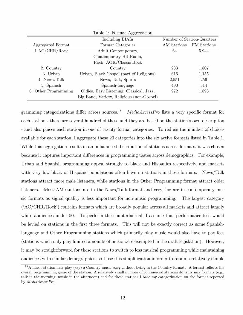
Table 1: Format AggregationIncluding BIAfn Number of Station-Quarters

Aggregated Format Format Categories AM Stations FM Stations1 AC/CHR/Rock Adult Contemporary, 64 5,944

Contemporary Hit Radio,Rock, AOR/Classic Rock

2. Country Country 233 1,8073. Urban Urban, Black Gospel (part of Religious) 616 1,155

4. News/Talk News, Talk, Sports 2,551 2565. Spanish Spanish-language 490 514

6. Other Programming Oldies, Easy Listening, Classical, Jazz, 972 1,893Big Band, Variety, Religious (non-Gospel)

gramming categorizations di¤er across sources.18 MediaAccessPro lists a very speci�c format for

each station - there are several hundred of these and they are based on the station�s own description

- and also places each station in one of twenty format categories. To reduce the number of choices

available for each station, I aggregate these 20 categories into the six active formats listed in Table 1.

While this aggregation results in an unbalanced distribution of stations across formats, it was chosen

because it captures important di¤erences in programming tastes across demographics. For example,

Urban and Spanish programming appeal strongly to black and Hispanics respectively, and markets

with very low black or Hispanic populations often have no stations in these formats. News/Talk

stations attract more male listeners, while stations in the Other Programming format attract older

listeners. Most AM stations are in the News/Talk format and very few are in contemporary mu-

sic formats as signal quality is less important for non-music programming. The largest category

(�AC/CHR/Rock�) contains formats which are broadly popular across all markets and attract largely

white audiences under 50. To perform the counterfactual, I assume that performance fees would

be levied on stations in the �rst three formats. This will not be exactly correct as some Spanish-

language and Other Programming stations which primarily play music would also have to pay fees

(stations which only play limited amounts of music were exempted in the draft legislation). However,

it may be straightforward for these stations to switch to less musical programming while maintaining

audiences with similar demographics, so I use this simpli�cation in order to retain a relatively simple

18A music station may play (say) a Country music song without being in the Country format. A format re�ects theoverall programming genre of the station. A relatively small number of commercial stations do truly mix formats (e.g.,talk in the morning, music in the afternoon) and for these stations I base my categorization on the format reportedby MediaAccessPro.

12

format structure. Stations observed as o¤-air are placed in the non-active �Dark�format, and I place

stations that enter during the data into the Dark format in the period before they are �rst on-air.19

Stations in the same market-format can have quite di¤erent market shares. I allow for these

di¤erences to be explained by several observable variables, speci�cally AM band*format interactions,

the proportion of the market�s population covered by the station�s signal (interacted with the station�s

band), an �out of market�dummy for whether the station is based outside the geographic boundaries

of the local market (e.g., in the surrounding countryside) and a dummy for whether the station has

an imputed share in one or more periods. With the exception of the format interactions, �rms treat

these characteristics as permanent and �xed. While this ignores the possibility of physical capital

investment, it is a reasonable approximation to the data where less than 1% of stations change signal

strength or tower height between 2002 and 2006. MediaAccessPro provides data on current and

historical station ownership. I assign ownership to the �rm that owns the station at the end of the

period.

2.4 Summary Statistics and Stylized Facts

Table 2 contains summary statistics on the market and station variables. The sample markets di¤er

widely in their populations, racial composition, total revenues and number of stations. Average

revenues per capita also vary across markets (mean $68.20, standard deviation $16.59, minimum

$34.76, maximum $116.97). On average, a �rm operates 2.5 stations, with the number varying from

1 to 8. Market shares and revenues also di¤er signi�cantly across stations within a market: in both

cases, within-market standard deviations are greater than between market standard deviations. For

this reason it is important to allow for both observed and unobserved heterogeneity in station quality.

The top section of Table 3 provides some summary statistics on format switching, based on the

sample markets. The years 2002-5 are used in estimation, but the table shows statistics for 1996�

2000 and 2001 as a comparison. Throughout the decade, 3-4% of stations switch formats per period.

The switching rates are similar across small and large markets, even though average station revenues

are almost 4.5 times larger in the large market group. This suggests that format repositioning costs

may also be larger in larger markets. Independent stations are slightly more likely to switch than

19This treatment will obviously a¤ect the estimated level of costs for moves from Dark to active formats. However, itshould not directly a¤ect the estimates of the costs of switching between active formats which are key for the analysis.

13

Table2:SummaryStatistics

MarketCharacteristics

Variable

Observations

Mean

Std.Dev.Min.

Max.

(market-periods)

Numberofstationsinmarket

714

23.2

5.8

1138

Numberofdi¤erentstationownersinmarket

714

9.4

3.2

318

Population(12andabove,inmillions)

714

0.733

0.747

0.055

3.683

Proportionofpopulationblack

714

0.119

0.124

0.002

0.502

ProportionofpopulationHispanic

714

0.091

0.130

0.005

0.793

Combinedlisteningtosamplestations(%

oftotalmarket20)

714

37.2

3.5

24.9

47.9

BIAfnEstimatedAnnualMarketAdvertisingRevenues(2002-2005,$m.)

408

53.5

66.0

3.9

403.7

StationCharacteristics

Variable

Observations

Mean

Std.Dev.Min.

Max.

(station-periods)

Marketshare(includesdarkstations)

16,543

1.6%

1.4%

011.3%

BIAfnEstimatedAdvertisingrevenues(station-year2002-2004,$000s)

6,413

2,438

3,702

2545,550

Dummyforstationlocatedoutsidemarketboundaries

16,543

0.061

0.240

01

DummyforAMband

16,543

0.299

0.458

01

Proportionofmarketcoveredbysignal(outofmarketstationsexcluded)21

15,526

0.786

0.358

0.003

1.1

Dummyforstationhasimputedmarketshareinatleastonequarter

16,543

0.147

0.354

01

Thetotalmarketincludestheoutsidegoodofnotlisteningtoradioandlisteningtonon-commercialandcommercialnon-samplestations.Market

de�nitionallowsforeachindividualtospendupto6hourslisteningtotheradiobetween6amandmidnight.

Signalcoverageisde�nedrelativetothemarketpopulationandIcapitat1.1toaddressoutliersthatappearedtodistortthedemandestimates.

14

Table3:SummaryStatisticsonFormatSwitchingandOwnership

FormatSwitching 1996-2000

2001

2002

2003

2004

2005

FormatSwitchingRate(perstation-quarter)

4.0%

3.4%

3.0%

3.7%

2.9%

3.4%

FormatSwitchingRateinMarketswith2001Population>1million

3.3%

3.9%

2.7%

3.4%

2.5%

4.3%

FormatSwitchingRateinMarketswith2001Population

�1million

4.3%

3.1%

3.2%

3.8%

3.1%

2.9%

Mean(Std.Dev.)MarketShareforSwitchingStation

50.4%

45.8%

54.3%

67.0%

56.6%

63.5%

as%ofmarketaverageshare

(51.8%)

(50.8%)(52.9%)(70.8%)(52.0%)(53.1%)

SwitchingRateforIndependentStations

4.8%

5.4%

4.2%

4.1%

3.9%

4.0%

SwitchingRateforStationsinLocalClusterswith2-3Stations

4.0%

3.5%

2.4%

3.0%

2.3%

2.0%

SwitchingRateforStationsinLocalClustersof>3Stations

3.4%

2.6%

2.8%

3.8%

2.8%

3.2%

Ownership

1996-2000

2001

2002

2003

2004

2005

%ofStationsA¤ectedByOwnershipChanges

16.1%

17.2%

5.8%

5.8%

6.1%

4.6%

MeanLocalMarketOwnershipConcentration(HHI,audienceshares)

0.249

0.274

0.276

0.275

0.286

0.287

ProbabilitythatTwoRandomlyChosenStationsareintheSameFormat:

StationsinSameLocalMarketwithDi¤erentOwners

0.20

0.21

0.22

0.22

0.21

0.21

StationsinSameLocalMarketwithSameOwner

0.28

0.28

0.29

0.29

0.29

0.29

StationsinDi¤erentLocalMarketswithDi¤erentOwners

0.20

0.21

0.22

0.21

0.21

0.21

StationsinDi¤erentLocalMarketswithSameOwner

0.27

0.28

0.28

0.29

0.29

0.28

15

Figure 1: Distribution of Year-to-Year Changes in Market Share (Listeners) for Switching and Non-Switching Stations

­3 ­2 ­1 0 1 2 3 4 50

0.2

0.4

0.6

0.8

1

1.2

1.4

Share Change in One Year (Percentage Point)

Ker

nel D

ensi

ty E

stim

ate

Switching StationNon­Switching Station

stations owned by multi-station �rms.

The bottom section of the table provides some additional information about ownership. During

the sample years, fewer stations changed ownership than in earlier years. Randomly selected pairs

of stations owned by the same �rm are more likely to be in the same format, which suggests that

economies of scope may be realized by operating similar stations. This is true whether one looks at

pairs of stations in the same market or di¤erent markets, suggesting that economies of scope from

operating similar stations may exist at both levels.

Figure 1 shows how the market shares of stations which switch formats change in the following

year, compared with stations that do not switch. Switching stations tend to gain listeners, and the

average gain is 32% of the average pre-switch market share. It is also interesting to note that few

switching stations experience large declines in market shares. This fact favors a model where station

quality can be predictably transferred across formats, rather than a model where stations receive

completely new, and unpredictable, draws on quality when they switch.

Table 4 shows the frequency with which switches are made between pairs of active formats. In all

formats, stations are much more likely to remain than to switch. Stations leaving News/Talk, Other

Programming or Spanish are more likely to switch to another non-music format, which re�ects the

16

Table 4: Format Switching Matrixformat in period t+ 1

AC Country Urban/Gospel News/Talk Other Prog. SpanishAC/CHR/Rock 0.975 0.004 0.005 0.003 0.009 0.002

format Country 0.013 0.963 0.003 0.007 0.005 0.006in period Urban/Gospel 0.007 0.003 0.974 0.008 0.005 0.003

t News/Talk 0.003 0.003 0.001 0.982 0.006 0.004Other Programming 0.023 0.007 0.006 0.014 0.941 0.006

Spanish 0.003 0.002 0.001 0.008 0.004 0.982

behavior of AM stations, but otherwise there are few obvious patterns. In estimation I will assume

that the cost of switching between any pair of active formats is the same, although this cost may

vary across stations and markets.

3 Model

In this section I describe the empirical model, and discuss the rationale for some of the restrictive

assumptions that I make.

3.1 Overview and Notation

Stations are observed in a set of local markets m = 1; :::;M; and play an in�nite horizon discrete

time game with periods t = 1; :::;1. A market has observable characteristics Xmt which include

population size, demographic composition based on 18 age-gender-race/ethnicity groups, population

growth rates and the value of each listener to advertisers. The players are a set of �local �rms�

o = 1; :::O. o owns a set of stations So in a particular local market m(o). As noted in the

Introduction, �rms optimize assuming that the current period�s ownership structure will remain the

same in the future so that any ownership changes that occur would be unexpected surprises. Stations

owned by the same company (e.g., Clear Channel) in di¤erent local markets will be controlled by

separate players in my game, but I explain below how I allow for cross-market economies of scope to

a¤ect format choices. Each station has observable characteristics Xst. Characteristics such as signal

coverage and whether the station is located outside market boundaries will be treated as �xed while

the band-format interactions can vary with format choices. Each station also has a one-dimensional

17

level of time-varying quality �st that is orthogonal to these observed characteristics. Xst and �st

capture vertical di¤erentiation between stations.

The set of players and stations are assumed to remain the same over time, so that there is no

new entry, permanent exit or changes in ownership. Each period local �rms generate revenues by

selling their stations�audiences to advertisers, and pay �xed costs so that their stations can operate.

Station audiences are determined by the size and demographic make-up of the market, station quality

characteristics (vertical di¤erentiation) and station programming formats (horizontal di¤erentiation).

There are F = 0; 1; :::; 6 discrete formats, where format 0 is the Dark (temporarily o¤-air) format.

Each station is in exactly one format each period, where Fst is a vector which indicates the format

of station s. To describe economies of scope from operating stations in the same format, F o;m(o)ft will

be a count of the number of local stations that o has in format f , and F o;m0

ft will be a count of the

number of stations in format f and market m0 that have the same corporate owner as o. The Xmt,

Xst; �st and ownership and format variables in all markets are observed by all �rms andMt denotes

these features of the state space at time t.

In the game, �rms choose the formats of their stations for the next period (they are not able

to take any other type of action). Aot denotes the discrete set of actions (next period choices)

available to o, and aot the chosen action. To place a limit on the size of the choice sets, I assume

that each �rm can move at most one station per period. Each possible action is associated with

a private information, iid payo¤ shock "ot(aot; �"o(Mt)). These shocks will be distributed Type

1 extreme value with location parameter 0 and scale parameter �"o(Mt) which can depend on o�s

observed characteristics. Market demographics and the �sts, which are continuous state variables,

evolve stochastically over time according to AR(1) processes and �rms cannot a¤ect how they evolve,

except that �st can change discretely when a format switch is made. Advertising values and listener

preferences are assumed to stay the same over time.

3.2 Timing

Within each period t; the timing of the game is as follows:

1. �rms observeMt;

2. �rms pay �xed costs Co(Mt)�C for the current period (i.e., a function of state variables that

18

are linear in parameters). These costs are a¤ected by local and cross-market economies of

scope;

3. �rms observe the private information shocks "ot to their payo¤s from each choice and simulta-

neously and irreversibly make their choices aot;

4. �rms receive revenuesP

s2So Rs(Mtj ), pay any repositioning costsWo(aot;Mt)�W and receive

the payo¤ shock "ot(aot; �"o(Mt)) associated with their format choices. are parameters of

the static listener demand system and advertising revenue functions. These parameters can

be estimated separately from the various � parameters that are estimated using the dynamic

model. A �rm�s total current period payo¤s are therefore

�ot(aot;Mt; �; ) + "ot(aot; �"o(Mt)) (1)

=Xs2So

Rs(Mtj )| {z }Period t Advertising Revenues

� Co(Mt)�C| {z }

Fixed Operating Costs

�Wo(aot;Mt)�W| {z }

Repositioning Costs

+ "ot(aot; �"o(Mt))| {z }

Payo¤ Shock For aot

5. Mt evolves to Mt+1, re�ecting �rms�format choices, and the stochastic evolution of market

demographics and station qualities.

3.3 Components of the Per-Period Payo¤ Function

I now describe each component of the payo¤ function.

3.3.1 Station Revenues (Rs(Mtj ))

A station�s revenues are determined by a listener demand model, which determines howmany listeners

a station has in each demographic group, and a revenue function, which determines the value of each

listener to the station.

Listener Demand A station�s audience in each of 18 demographic groups is determined by a

static, discrete choice random coe¢ cients logit model as a function of the state variables in its own

market. Each consumer i in this market chooses at most one station, and i�s utility if she listens to

19

non-Dark station s is

uist = Xst S + Fst(

F + Fi ) + �st + "List (2)

= �st(Fst; Xst; S; F ; �st) + Fst

Fi + "List (3)

where �st is the �mean utility�of the station for a consumer with baseline demographics (white, male,

aged 12-24) and "List is an iid logit shock to individual preferences. Xst and �st are assumed to enter

the preferences of all consumers in the same way. �st allows stations with the same observed charac-

teristics to have di¤erent market shares, and while it is orthogonal to observed market characteristics,

the values of �st can be backed out from the estimated demand model. F are the average format

tastes of baseline consumers. Individual deviations from these preferences are

Fi = FDDi + �vFi (4)

where the �rst term re�ects systematic demographic preferences (additively separable age, ethnicity

and gender e¤ects) and vFi is a vector of draws from independent standard normals. The parameter

� determines the heterogeneity in format preferences within a demographic group, and it is assumed

to be the same across formats. A consumer receives utility of "Li0t if she chooses the outside good

(i.e., she does not listen to one of the commercial radio stations in my model).

This is a rich speci�cation, but it makes two signi�cant simpli�cations. First, consumers are

assumed to choose at most one station, whereas in reality people listen to several stations for di¤erent

lengths of time during a period (ratings quarter). This is a common simpli�cation when using

aggregate data (e.g., Nevo (2001)) and it can be rationalized as a representation of consumers�

preferences during shorter time periods, which are aggregated to give period market shares. This

representation is adequate if stations and advertisers are indi¤erent between audiences of the same

size made up of either a few people who listen a lot, or a lot of people who listen a little, and this

is consistent with average quarter hour (AQH) shares being the ratings number that are most used

by advertisers. Second, the model is entirely static, whereas listening habits might make shares

adjust slowly to quality or format changes. This simpli�cation seems reasonable given my focus on

major format changes, which are likely to cause any listener to change her habits, and six-month

time periods, which are likely to be longer than the time required for listeners to adjust.

20

Revenues Per Listener I assume that station s�s revenues for a listener with demographics Dd

are determined by a parametric function

rsmt(Dd) = m(1 + Ysmt Y )(1 +Dd d) (5)

where m is a market �xed e¤ect and d allows listeners with di¤erent characteristics to be more

or less valued by advertisers. In order to allow for format switching and market structure to a¤ect

revenues, the variables in Y include the number of other stations that the �rm has in the format, the

number of other stations in the format and a dummy variable for whether the station switched formats

in the previous period. I also allow for revenues per listener to depend on the station�s aggregate

market share, as work in the broadcast television industry has shown that larger stations achieve

higher revenues per viewer per minute of commercial time (Fisher et al. (1980)). Total station

revenues Rs(Mtj ) are calculated by multiplying the number of listeners in each demographic group

by these prices.

3.3.2 Repositioning Costs (Wo(aot;Mt)�W )

A local �rm has to pay a repositioning cost when it moves a station to a new format. I allow

repositioning costs to depend on whether the potential move is between active formats or to or from

the Dark format, total market revenues22, the revenues of the station being moved and whether the

station switched formats in the previous period. Because I estimate a cost for all possible moves, it

is not possible to also estimate a common �xed cost that stations pay to be active.23

3.3.3 Fixed Costs and Economies of Scope (Co(Mt)�C)

I assume that active stations pay �xed costs. The level of costs that is common across formats is

not identi�ed, but, using the positioning decisions of multi-station �rms, I can estimate the value of

22Speci�cally this variable equals market revenues per percentage point of radio listening during the years that themarket is observed in the data. Results using total population are similar, but I prefer the revenue measure as itshould also re�ect some di¤erences in input prices across markets, as well as population.23One could assume that the cost of switching to Dark is zero and then estimate the �xed cost of being active.

However, switches to Dark are rare, so that estimated �xed costs could be negative. Instead, I estimate a cost ofswitching to Dark which can be interpreted as a re�ection of the fact that when a station goes o¤-air it will lose thegoodwill of all of its existing listeners and advertisers, not just those who would leave the station if it switched to adi¤erent active format.

21

economies of scope that arise when a �rm operates several stations in the same format. For local

market economies of scope, I allow each station�s �xed costs to fall linearly with the number of other

stations that the local �rm has in the same format. These should re�ect e¢ ciencies achieved in pro-

gramming and selling commercials to advertisers with similar preferences. Cross-market economies

of scope are modelled with a non-linear speci�cation because the number of a¢ liated stations in other

markets can be very large (maximum in the data is 232). I assume that a local �rm is rewarded (by

the corporate owner) for the contemporaneous externality that its format con�guration has for local

�rms in other markets, and, taking this into account, o�s total bene�t from cross-market economies

of scope is proportional to24

Xf

0BBBBBB@Fo;m(o)ft log

�1 + F oft � F

o;m(o)ft

�| {z }cost reduction for local �rm�s own stations

+

Xj 6=m(o)

F o;jft

�log(1 + F oft � F o;jft )� log(1 + F oft � F o;jft � F

o;m(o)ft )

�| {z }

externality on stations in other markets with the same corporate owner

1CCCCCCA (6)

where F o;m(o)ft is the number of stations o has in format f in its own market in period t, and F oft =

Fo;m(o)ft +

P8j 6=m(o) F

o;jft is the total number of stations across markets in format f with the same

corporate owner.

3.3.4 Payo¤ Shocks ("ot(aot; �"o(Mt)))

Firms receive iid (across �rms and over time) private information shocks to their payo¤s from each

possible format choice, including keeping stations in the same format. These shocks are drawn from

a Type 1 extreme value distribution with location parameter 0 and scale parameter �"o(Mt): The

scale parameter is identi�ed in my setting because revenues are treated as observed and all costs are

assumed to be �xed. I allow the scale parameter to depend on both a constant and the revenues of

the local �rm in the current period.25 The revenue e¤ect should be identi�ed by how much �rms

24See Aguirregibiria and Ho (2009) for an alternative, and still fairly simple, way to model network externalities,applied to the airline industry. Note that I calculate this function based on only the sample markets.25It is important to allow for the scale of the payo¤ shocks to vary across �rms because �rms have quite di¤erent

expected future revenues depending on the size of the market and the number and quality of stations owned. With noscaling, choice probabilities exceptionally close to 0 or 1 tend to be predicted for either high or low revenue �rms. Ihave also experimented with allowing the scale of the shocks to also depend directly on the number of stations owned.Unfortunately the pseudo-likelihood minimization procedure often performed poorly in this case.

22

with di¤erent revenues tend to switch and how predictable their chosen format switches are (based

on predicted future values).26 The interpretation of these payo¤ shocks are factors that a¤ect the

format choices of �rms that are not captured by expected revenues or costs. For example, the �rm

described in Section 1.2 was attracted to Sports partly because the �rm had some non-radio interests

in managing sports facilities so it knew more about the types of advertisers that might be attracted

to a Sports station. The assumptions that payo¤ shocks are private information and independent

over time (serial independence) are necessary for tractability. The example does provides anecdotal

support for the private information assumption by illustrating how �rms may want to keep their

intentions hidden from competitors.27

3.4 Evolution of the State Variables

At the end of period t, the state variables evolve for the following period. Station formats change

deterministically with �rms�choices. Unobserved station quality is assumed to evolve according to

an AR(1) process with normally distributed innovations that are iid across stations

�st = ���st�1 + ��st if Fst = Fst+1 (7)

= ���st�1 + ��st � � if Fst 6= Fst+1 (8)

where ��st � N(0; �2v�): The � term allows for a change in station quality when it changes format.

An important assumption, which allows consistent �rst-stage estimation of the demand model when

format choices are endogenous to qualities, is that no �rm knows the v�st+1 innovations when they

make format choices in period t, so that there can be no selection into di¤erent formats based on

these innovations. In contrast, there can be selection based on the prior level of the �s. I show that

this model of quality innovations allows me to match the distribution of observed share changes in the

data. If it was assumed that �rms knew the innovations in quality when choosing these formats, it

would be necessary to adopt a di¤erent approach to estimation of listener demand, possibly involving

26Note that I assume that repositioning costs vary with the current revenues of the station that would be moved(which can therefore di¤er across choices), not the current total revenues of the �rm (that are common across choices).27A standard objection to the private information assumption in static models (e.g., Seim (2006)) is that it can lead

to �rms experiencing ex-post regret, because, for example, more �rms choose the same location than was expected.However, in my model the rate of switching is relatively low and in the data it is relatively rare for two �rms in thesame market to make switches that would have a large impact on the expected pro�tability of each other�s switch. Ina dynamic model �rms are also able to quickly reverse choices that turn out to be particularly sub-optimal.

23

the joint estimation of the demand and format choice models which would create an exceptionally

large computational burden.

While listener demand depends on 18 mutually exclusive age-gender-ethnic/racial groups it is

cumbersome to model the evolution of each of these groups independently. Instead, I model the

growth rate for each ethnic/racial group (white, black and Hispanic) and assume that the same

growth rate applies to each of the associated age-gender groups. I assume that for ethnic group e

log

�popmetpopmet�1

�= � 0 + � 1 log

�popmetpopmet�1

�+ umet (9)

which allows population growth for particular groups to have the serial correlation that we observe in

the data.28 This particular speci�cation also lets me address the problem that population estimates

are annual.

3.5 Value Functions and Equilibrium Concept

Following the empirical literature on dynamic games, I assume that �rms play a stationary and

anonymous pure strategy Markov Perfect Nash Equilibrium (MPNE).29 A stationary Markov Perfect

strategy �o is a mapping from (Mt; "ot) to actions aot that does not depend on t; and � is the set

of strategies for all �rms in all states. V �o (Mt; "ot) de�nes a �rm�s value in a particular state when

it uses an optimal strategy and other �rms use strategies de�ned in �. Dropping notation for the

parameters, by Bellman�s optimality principle

V �o (Mt; "ot) = max

aot2Aot

24 �(aot;Mt) + "ot(aot;Mt)+

�RV �o (Mt+1)g(Mt+1jaot;��o;Mt)dMt+1

35 (10)

28Alho and Spencer (2005), Chapter 7 discuss the application of time series models, including AR(1) to demographicgrowth rates. Models with additional lag terms would complicate the state space of the dynamic model.29With continuous states it is an assumption that a pure strategy MPNE exists. Dorazelski and Satterthwaite

(2010) show the existence of a pure strategy MPNE for a model with discrete states when the random component ofpayo¤s has unbounded support. Conceptually it would be possible to convert my model into one with an exceptionallylarge number of discrete states using an arbitrarily �ne discretization. A similar argument is made in Jenkins et al.(2004).

24

where � is the discount factor. The choice-speci�c value function v�o (aot;Mt) de�nes o�s expected

payo¤ from choosing aot excluding the idiosyncratic shock component "ot(aot;Mt)

v�o (aot;Mt) = �(aot;Mt) + �

ZV �o (Mt+1)g(Mt+1jcot;��o;Mt)dMt+1 (11)

It follows that o�s optimal strategy ��o in state (Mt; "ot) when other �rms use ��o is

��o(Mt; "ot;��o) = arg maxaot2Aot

[v�o (aot;Mt) + "ot(aot;Mt)] (12)

Strategies will form a MPNE when, in all states, the strategy of each �rm maximizes its value given

the strategies of other �rms.

3.6 Discussion of the Assumptions

Several assumptions deserve some additional comment.

Time E¤ects. When estimating the listener demand and revenue models I allow for time

e¤ects as, during the sample period, there is a downward trend in radio listenership (which began

in the late 1980s) and an upward trend in revenues per listener. Unfortunately it is di¢ cult to

include persistent trends in in�nite horizon dynamic games because existing solution methods assume

stationarity. Therefore I assume that �rms expect that the current value of the time e¤ects will

remain �xed in the future (so, for example, �rms in Spring 2003 assume that the Spring 2003 values

of the time e¤ect of listener demand and per listener revenues will persist into the future and the

�rms in Spring 2004 assume that the Spring 2004 values will persist into the future). This is a

simpli�cation but it is consistent with the fact that total revenues, which is what �rms care about,

were stable during the sample period changing by no more than 2% from year-to-year, because the

trends in listenership and revenues per listener roughly cancelled out.30 ;31

30The Radio Advertising Bureau estimates annual industry revenues from 2002 to 2006 of $19.4 bn., $19.6 bn., $20.0bn. and $20.1 bn (personal correspondance, November 29, 2010).31Given my counterfactual, it is important that these trends are common across formats. This appears to be the

case in the data. For example, based on Arbitron�s Radio Today reports time spent listening between 2001 and 2005fell by 4.9% for the population as a whole, 5.1% for black listeners and 3.5% for Hispanic listeners who were beingserved by many more Spanish language stations over this period. When I regress station revenues per listener onformat dummies, market dummies, year dummies and year*format interactions, the coe¢ cients on the year*formatinteractions are jointly insigni�cant (p-value 0.3142) which suggests that revenues per listener were changing in asimilar way across formats over time.

25

Entry and Exit. As noted in Section 2, de novo entry and exit are very rarely observed, and

the issuing of new licenses is complicated by spectrum constraints in most markets, so I choose not

to include these margins in my model (although stations can go o¤-air temporarily). Of course, very

large fees might cause some stations to exit rather than switch to non-music programming. However,

even when industry revenues dropped dramatically after 2008, the FCC still reported excess demand

for broadcast licenses (US GAO (2010), p. 25).

One Move Per Period. The current model assumes that a local �rm can only move at most

one station per period in order to limit the number of choices available to a particular �rm. While

99.5% of �rm-period observations satisfy this constraint, there are 28 observations where �rms move

two stations and 1 observation where a �rm moves 3 stations.32 These observations are ignored

when calculating the pseudo-likelihood as part of the estimation process, and it is assumed that all

other local �rms optimize assuming that other �rms can only move one station at once. Relaxing

this restriction in the dynamic model with seven formats would be very burdensome, but I have

investigated how allowing each �rm to make two moves, rather than one move, a¤ects the results in

a two-period version of the model where �rms only care about their revenues in the following period.

The only signi�cant change is that the estimates of local economies of scope increase by around 10%,

which is sensible as 9 out of the 28 two move observations involve a �rm moving two stations to the

same format at the same time.

Coordination Across Local Firms with the Same Corporate Owner. I assume that

format choices are made by local �rms, but that each �rm is compensated for how its current format

con�guration a¤ects the �xed costs of �rms in other markets. This provides a relatively simple

way to allow for cross-market economies of scope to a¤ect format choices, without modelling a single

decision maker who controls many stations simultaneously. However, it does assume that local �rms

with the same corporate owner do not know each others " draws, so that they cannot coordinate their

simultaneous choices. Instead, �rms have expectations about what their sister �rms will choose in

the same way that they have expectations about their competitors.

32There are 364 �rm-market observations where exactly one station is moved.

26

4 Approximately Solving the Model using Parametric Pol-

icy Function Iteration (PPI)

Finding an exact solution to the proposed model, which has many asymmetric players and a rich state

space that is a mixture of continuous and discrete variables is beyond the current literature.33 Instead,

I employ the technique of �parametric policy function iteration�(PPI) to compute an approximate

solution. This section describes how I use PPI to solve the model, and brie�y describes the related

Monte Carlo experiments that are detailed in the Appendix. Estimation is described in the next

section.

Following AM, it is convenient to express �rms�strategies in probability space. De�ne P � as the

probabilities that actions are chosen prior to the "s being revealed when �rms use strategies �

P �o (aot;Mt) =

ZI(�o(Mt; "ot) = aot)hot(Mt; "ot)d"ot (13)

where hot("ot) is the pdf of the vector of shocks "ot and I(�o(Mt; "ot) = aot) is an indicator for action

aot being chosen. Equilibrium strategies �� imply equilibrium choice probabilities P �. At P �, we

can express ex ante (i.e., before the "s are revealed) value functions as

V P �

o (Mt) = e�o(Mt; P�) + �

ZV P �

o (Mt+1)g(Mt+1jP �;Mt)dMt+1 (14)

where e�o(Mt; P�t ) are o�s expected �ow pro�ts for strategies P � and state Mt. In terms of the

within-period timing detailed above, expected �ow pro�ts are calculated from stage 3 in the current

period to stage 2 in the following period, so they include next period�s expected �xed costs (which

will depend on the actions chosen in the current period). For describing estimation later, it is useful

33To understand the size of the state space, suppose that cross-market e¤ects are ignored and consider a marketwith 20 stations, with time-varying station quality discretized to 5 levels and 25 discretized states describing marketdemographic composition. Then, the number of possible states for this market would be greater than 3.8e31, and be-cause stations di¤er in some permanent characteristics the number of states could not be reduced using exchangeability(Gowrisankaran (1999)).

27

to express e�o(Mt; P�ot) as

e�(Mt; P�ot) =

Xaot2Aot

P �ot(aotjMt;��o)

0BBB@P

s2So Rs(Mtj )�Wo(aot;Mt)�W�

�RCo(aot;Mt+1)�

Cg(Mt+1jP �;Mt)dMt+1

+e(aot; P�ot; �

"o(Mt))

1CCCA (15)

where e(aot; P �ot; �"ot(Mt)) = �"o(Mt)({ � log(P �(aotjMt;��o))) is the expected value of the " associ-

ated with choice aot. { is Euler�s constant. Note that e only depends on o�s own choice probabilities

in the current period, and not the strategies of other �rms or o�s own strategy in future periods.

Fixed costs in the next period can depend on the choices of other �rms in di¤erent markets because

of national economies of scope.

Stacking states and �rms, equation (14) can be expressed in matrix form as

V P � = e�(P �) + �EP �VP � (16)

where EP � is the Markov operator corresponding to policies P �; and for a particular state and �rm

EP �VP �

o (Mt) =

ZV P �

o (Mt+1)g(Mt+1jP �;Mt)dMt+1 (17)

Holding P � �xed, equation (16) has a unique solution for V P � de�ned by the linear equations

V P � = [I � �EP � ]�1e�(P �) (18)

Policy iteration seeks to solve for equilibrium policies and values by iterating two steps (Judd

(1998), Rust (2000)). At iteration i, in the �rst step (policy valuation), (15) and (18) are applied to

calculate values V P i associated with probabilities P i that may not be optimal. In the second step

(policy improvement), values V P i are used to update P i by computing choice-speci�c value functions

vPi

o (aot;Mt) = �(Mt; aot) + �

ZV P i

o (Mt+1)g(Mt+1jP i;Mt; aot)dMt+1 (19)

where g(Mt+1jP i;Mt; aot) is the probability of transitioning toMt+1 when o chooses aot. P i+1 is

calculated using formulae implied by the Type 1 extreme value distribution of the "s where the scale

28

parameter is �"o

P i+1ot (aotjMt; Pi) =

exp

�vP

io (aot;Mt)�"o(Mt)

�P

a0ot2Aotexp

�vPio (a0ot;Mt)

�"o(Mt)

� (20)

For V P s and P s that constitute a �xed point of these equations, the associated strategies will con-

stitute a Markov Perfect Nash equilibrium. Similarly, for any Markov Perfect Nash equilibrium

strategies, the V P s and P s will form a �xed point. For a game, there may be multiple solutions and

convergence of policy iteration is not guaranteed. Practical implementation of policy iteration with

continuous states requires a choice of N discrete states at which to evaluate V and P and, typically, a

method for approximating the integrals by choosing an additional set of statesMt+1 for eachMt.34

Parametric Policy Function Iteration (PPI).

To apply parametric policy iteration I make the further assumption that the value function can

be approximated using a linear combination of K basis functions describing the state variables

V P �

o (Mt) 'KXk=1

�k�ko(Mt) (21)

so that equation (14) can be expressed as

KXk=1

�k�ko(Mt) ' e�(Mt; P�ot) + �

Z KXk=1

�k�ko(Mt+1)g(Mt+1jP �;Mt)dMt+1 (22)

The solution to the value function for given choice probabilities now requires �nding K � coe¢ cients

rather than values for V at each state. When the equations (22) are stacked into matrix form for N

states

�� = e�(P �) + �E�� (23)

where � is the matrix of basis functions and E� is a matrix where element (j; k)

E�j;k =

Z�ko(Mt+1)g(Mt+1jP �;Mt)dMt+1 (24)

34The integration method must specify the discrete set of statesMt+1 for eachMt at which to evaluate V , a methodfor approximating V (Mt+1) given the estimates of V at the N points, and a rule for weighting the V (Mt+1) estimatesthat are calculated to approximate the integral.

29

if row j is associated with �rm o and stateMt. For the overidenti�ed case (N > K), b� can be foundusing the OLS estimator

b� = ((�� �E�)0(�� �E�))�1(�� �E�)0e�(P �) (25)

The iterative procedure now consists of the following steps for a given initial set of choice probabilities

P i:

1. at a given set of N states, calculate �; and use (24) to calculate the matrix E� and the vectore�(P i). Details of the approximate integration procedure are provided below;2. create matrices (�� �E�) and use (25) to calculate b�;3. use b� to calculate the choice-speci�c value functions for each choice

vPi

o (aot;Mt) = �(Mt; aot) + �KXk=1

��Z�ko(Mt+1)g(Mt+1jP i;Mt; aot)dMt+1

� b�k� (26)

4. use formulae (20) to calculate updated choice probabilities P 0; and calculate P i+1 = P 0 +

(1 � )P i, where the weights can vary (from 0.1 to 1) depending on how well the choice

probabilities appear to be converging. In practice, weights equal to 1 work �ne close to the

�nal values.

5. repeat steps 1-4 until the maximum di¤erence between P i and P 0 is small enough (less than

1e� 5).

Integration.

An e¢ cient procedure is required to perform the integrations. In particular it would very com-

putationally expensive to calculate entirely new matrices of variables each time a choice probability

changes: in my setting this would require solving a random coe¢ cient demand model. Instead, I

calculate matrices for many sets of moves by other �rms in advance, and reweight these matrices as

the choice probabilities change. Speci�cally suppose that for a given state inMt, I consider a set of

H statesMh;t+1 created by considering all possible combinations of moves by the current �rm, a set

of S� draws for innovations in � and market demographics (which do not depend on �rm choices),

30

S�o;m moves by other �rms in the same local market, and S�o;�m moves by other �rms with the same

corporate owner in di¤erent local markets. The integralR�ko(Mt+1)g(Mt+1jP �;Mt)dMt+1 is then

approximated byHXh=1

�ko(Mh;t+1)g(Mh;t+1jP �;Mt)PHh0=1 g(Mh0;t+1jP �;Mt)

A similar integration is used to calculate a �rm�s expected �xed costs in the following period. To

be accurate this integration procedure requires that the moves S�o;m and S�o;�m are those that are

likely to be made. I choose these moves by �rst solving (or estimating when the parameters are being

estimated) a model where �rms assume that all other �rms�formats will remain �xed forever. This

is a single agent model that can be solved quickly. The choice probabilities implied by this model are

then used to select the set of S�o;m moves by other �rms which are most likely. In estimating and

solving the model for the counterfactual I use S� = 50, S�o;m = 500 and S�o;�m = 100.35 To make

computation with this many simulations feasible I assume that variables describing cross-market

factors enterPK

k=1 �k�ko(Mt) completely separably from the variables describing a �rm�s situation

within its own market. It is also possible to repeat the procedure by drawing a new set of states

S�o;m and S�o;�m that re�ect the choice probabilities of a solved game.

Speci�cation of the Parametric Function.

It is necessary to specify the variables used in the parametric approximation of the value function

and the initial set of N states at which the value function is evaluated. The N states used are

the ones that are observed in the data (a total of 6,075, one for each local �rm-period observation).

These points will, of course, represent the types of states that are likely to be observed given �rms�

equilibrium strategies. In the Monte Carlo described in the Appendix, using additional states, which

increases the computational burden, gives, at most, a small improvement in performance.

There are 151 variables used in the parametric approximation that can be divided into 6 groups (a

full list and code to calculate them is available). The �rst group describe market characteristics: the

proportion black and proportion Hispanic in the market�s current population, market population and

market average revenues per market share point, and several interactions between these variables.

The second group contains measures of the quality of stations owned by the �rm: sums of exp(�st)

(which can be recovered from the estimated demand model), exp(Xs b s), the interaction of these35S�o;m and S�o;�m are obviously capped at the maximum possible moves by other �rms that could be observed.

For example, for independent �rms S�o;�m is trivially equal to zero.

31

variables and interactions with a count of the number of stations owned and market average revenues

per market share point.

The third group contain similar variables for the two largest rival �rms that the �rm faces in its

market. The order is based on the number of stations owned and total current market share, so that

the identity of these leading rivals can change across periods.

The fourth group of variables provide some more detailed variables for individual formats. For

example, the number of the �rm�s stations in the News/Talk format, a count of how many of these

are AM band, and interacts these variables with the number of AM stations owned by rivals in that

format. For Urban and Spanish-language stations it includes the number of the �rm�s stations in

the format, and interacts them with the number of rival stations in the format and the proportion

of the population that is black or Hispanic respectively.

The �fth group are based directly on the �rm�s revenues. In particular it includes the �rm�s

current revenues, the �rm�s revenues if the time-varying components of quality � are set equal to

zero (which helps to capture �rms�long-run expected values), and several variables that capture how

the �rm�s revenues would change if it moved its stations to di¤erent formats assuming that other

�rms do not move their stations and station quality and demographic variables do not change (so

these variables are only functions of the current state variables, and can change across periods). For

example, these variables include a count of the number of moves that a �rm could make which would

increase its own revenues, and its interaction with the �rm�s current revenues and the number of

moves which would result in owning an increased numbers of stations in the same format.

The �nal group has variables that may a¤ect economies of scope including a count of the number

of stations the �rm has which are in formats with another one of its stations, an interaction of this

variable with market size and market average revenues per share point and the value of the national

economies of scope variable (de�ned in Section 3) for each format. The Monte Carlo experiments in

the Appendix consider speci�cations with both more and less variables than are used here.

Monte Carlo Experiments: Solution.

The Appendix describes a Monte Carlo exercise designed to assess whether this method can

accurately approximate the value function and accurately predict what will happen if performance

fees are introduced so that the revenues of all stations in a particular format are taxed. To do

this, I set-up a simpli�ed, purely discrete version of the model that can be solved exactly, but

32

which incorporates several of the key features of the full model, such as multi-station �rms and

heterogeneity in demographics and station qualities across markets, and, just like I do using the

data, I pool observations from di¤erent markets when applying PPI. I compare the accuracy of the

value function approximation and the implied choice probabilities using three speci�cations that di¤er

in how many variables are used to approximate the value function and the states used to evaluate

the approximations.

When there are no performance fees, I �nd that in all three speci�cations, the solution based on

the parametric approximations provides values and choice probabilities that are very close to those

from the model that is solved exactly (e.g., correlation coe¢ cients of 0.96 or higher). These high

correlations partly re�ect the fact that the various variables based on current revenues and potential

revenues in other formats, which are known (but complicated) functions of many state variables, can

capture a lot of the variation in �rm values. There is also evidence that simpler speci�cations of the

parametric value function approximation can actually work better, presumably because they avoid

problems of over�tting. All three speci�cations predict both the short-run and long-run e¤ects of

performance fees without signi�cant bias.

5 Estimation

I estimate the model in four stages. The steps involve the estimation of (i) the process governing

demographics; (ii) the listener demand model and the process for the � component of station quality;

(iii) the revenue function; and, (iv) the dynamic model.

5.1 Step 1: Demographics

The population of ethnic group e in market m is assumed to evolve according to the following process

log (popmet)� log(popmet�1) = � 0 + � 1 (log (popmet�1)� log(popmet�2)) + umet (27)

where pop is the level of population. Estimation is complicated by the fact that the County Popu-

lation Estimates are annual (July each year) so I only observe them every other period. However,

adding these di¤erenced equations for t and t�1 and substituting for (log (popmet�1)� log(popmet�3))

33

in the resulting equation gives

log (popmet)� log(popmet�2) = 2� 0(1 + � 1) + � 21 (log (popmet�2)� log(popmet�4)) + eumet (28)

where eumet = umet+(1+� 1)umet�1+� 1umet�2. The population numbers in this equation are observed,

but (log (popmet�2)� log(popmet�4)) will be correlated with eumet. I estimate (28) by 2SLS using

(log (popmet�4)� log(popmet�6)) as an instrument for (log (popmet�2)� log(popmet�4)).36 I estimate

this equation using data from all radio markets from 1996 to 2006, not just the sample of markets

used to estimate the rest of the model. The estimates are b� 0 = 0:00035 (0:00004) and b� 1 = 0:9535(0:0146) (standard errors in parentheses) respectively, and the standard deviation of the innovations

umet is 0.0125.

5.2 Step 2: Listener Demand Model and Evolution of Unobserved Sta-

tion Quality (�)

The listener demand model is a random coe¢ cients demand model with no price variable. There is

a potential endogeneity problem because station formats might be correlated with the components of

station quality (�) that are not associated with observed characteristics. To avoid the endogeneity

problem I form moments based on the innovations in station quality (v�) that are assumed to be

unknown when format choices are made, using my assumption that �st evolves according to an AR(1)

process (with serial correlation parameter ��). The model has 32 non-linear parameters (��, � and

30 demographic taste parameters) collectively labelled NL, and a set of linear parameters ( L) that

capture format tastes, time e¤ects and observable di¤erences in station quality. Estimation involves

minimizing a GMM objective function based on three sets of moments.

5.2.1 Quasi-Di¤erenced Moments

The quasi-di¤erenced moments are formed from the equations for listener mean utilities and the

process that determines the evolution of the component of station quality � that is not associated

36The instrument will be correlated with the endogenous variable if �1 6= 0 (serial correlation in population growthrates) and it should be uncorrelated with eumet if the innovations in growth rates are independent.

34

with observed station characteristics

�st � Xt t +Xs

S + Fst F + �st (29)

�st = ���st�1 � I(Fst 6= Fst�1) � + v�st; �

�st � N(0; �2v�) (30)

where I() is an indicator function and Xt are time dummies which I include in the empirical speci-

�cation of demand (see comments in Section 3). (30) assumes that quality evolves in the same way

whether or not a station switches formats, except for a �xed change �. This is a strong assump-

tion, so I proceed by forming quasi-di¤erenced moments based only on stations that do not change

formats, and calculate the value of � implied by how the �sts of switching stations change when I

assume these parameters and I examine how well this estimated process can match the distribution

of share changes for stations that do change formats. In practice, the distributions match closely so

that the assumption of a common process seems reasonable.

I form the moments by quasi-di¤erencing the mean utilities �st(q; NL); which are uniquely de�ned

by the observed market shares q and the non-linear parameters (Berry (1994), Berry et al. (1995))

��st = �st(q; NL)� ���st�1(q;

NL)� (1� ��)Xst S � (1� ��)Fst

F (31)

where I have exploited the fact that Xst = Xst�1 and Fst = Fst�1 for stations that remain in the

same format. The assumption that the quality innovations ��st are unknown when format choices

are made implies that ��st must be uncorrelated with Xst and Fst. I form the moments as

E(Z 0v�(��; NL; L)) = 0 (32)

where the v�s are de�ned by the above equation and the instrument matrix Z includes Xst; Fst and

an initial estimate of the lagged mean utilities, �st�1.37 Given values of �� and NL, the linear

coe¢ cients can be estimated from these moments using an OLS regression where the dependent

variable is �st(q; NL)� ���st(q; NL). �2v� is estimated using the residuals from this regression.

37These initial estimates were obtained by using lagged log(market share) as the instrument.

35

5.2.2 Demographic Moments

The accurate estimation of coe¢ cients for demographic tastes using aggregate market share data can

be aided by including additional demographic-speci�c moments (Petrin (2002)). I form this type of

moment based on the average demographic composition of the audience of di¤erent formats reported

in Arbitron�s annual Radio Today reports. Speci�cally these reports list the average proportion of a

format�s listeners who are in particular age (12-24, 25-49, 50 plus), gender and ethnic/racial (white,

black or Hispanic) categories based on a particular set of markets. I specify 30 moments (which

match the 30 demographic parameters) based on the di¤erence between these reported averages and

the averages predicted by my model for the quarters used by Arbitron and the set of markets that

are common to my sample and Arbitron�s calculations38

E(propARBftd � \propftd(�(q; NL); NL)) = 0

where prop is the proportion of a format�s listeners who are in a particular demographic group. The

demographic parameters will be identi�ed by how a format�s average demographics di¤er from what

would be expected given the demographics of markets which have stations in these formats.

5.2.3 One Additional Moment

The quasi-di¤erenced moment with instrument �st�1 and the demographic moments provide 31 mo-

ments for identifying 32 non-linear parameters. Intuitively, the parameter which lacks an obvious

identifying moment is � which determines the heterogeneity in listeners�preferences for particular

types of programming, and therefore how much listeners tend to substitute within formats, across

formats and with the outside good. Higher values of � imply that, all else equal, radio and for-

mat listening should increase more slowly with the number of stations in a market. To provide an

additional moment I assume that the expected value of �st, which could also a¤ect how audiences

increase with the number of stations in a market, is independent of market size (log population).39

38Arbitron uses di¤erent markets for its age/gender and ethnic calculations. There are some markets included inArbitron�s calculations which are not in my sample. I have veri�ed that the demographic taste coe¢ cients remainsimilar if I include all of the markets used by Arbitron in the demand estimation. Creating the moments requiresaggregating some of the formats used in Arbitron�s reports, which is done by weighting these formats by averagelistenership.39Speci�cally I assume that the vector of �st for stations that are based inside the market should be independent

of market size. The assumption would likely not hold for stations located outside of the market, as their signals are

36

Berry and Waldfogel (1999) make a similar use of market population as an instrument to identify

substitution patterns in a nested logit model of listener demand. Note that if �rms invest more in

station quality in larger markets, which is ignored in my model but which we might expect given the

di¢ culty of new entry, then this should tend to lead to � being underestimated. In practice, my

estimate of � is larger than those estimated in recent papers where this moment condition is not

included (Mooney (2010b) and Jeziorski (2010)).

5.2.4 Estimation Algorithm

The demand system is estimated by adapting the algorithms outlined by Berry et al. (1995) and

Nevo (2000). Prior to estimation, Halton draws for vF are made for 450 simulated individuals

equally spread amongst the 18 mutually exclusive demographic groups. The simulated individuals

in these groups are weighted during estimation by the size of the demographic group as a percentage

of the market�s population. For particular values of the non-linear parameters, the mean utilities (�)

are calculated using a contraction mapping procedure.40 These utilities are then used to form the

quasi-di¤erenced moments, allowing the calculation of the linear parameters. Analytic derivatives

are used to speed the search. My model is exactly identi�ed (the number of moments equals the

number of parameters), so the value of the objective function at the true parameters should be equal

to 0. Its value at my parameter estimates is less than 3e�10.41

5.3 Step 3: Revenue Model

The estimated revenue model assumes that station s�s revenues for a listener with demographics Dd

are

rst(Ys; Dd; ) = mt(1 + Ysmt Y )(1 +Dd

D) (33)

unlikely to cover the entire market area in larger markets (recall that I control for the signal coverage of the stationslocated inside the market).40The convergence tolerance is set to 1e-12:41Knittel and Metaxoglu (2008) and Dube et al. (2009) highlight that commonly used numerical routines for random

coe¢ cient demand models can fail to �nd the coe¢ cients that minimize the objective function. My use of an exactlyidenti�ed model allows me to check that I have found a global minimum up to numerical tolerance. I have estimatedmany di¤erent speci�cations of the random coe¢ cients model using this data. Convergence problems were sometimesencountered when format-speci�c �f parameters were included along with additional moments, and they occurredwhen one or more of these parameters was close to zero. Even when the parameter estimates for these models didappear to converge successfully the estimates for these parameters were imprecise.

37

where mt are market-year e¤ects. For estimation, I assume that the mean annual revenues per

listener for a station reported by BIAfn equal

rBIAsy =

Xt2y

X8d

rst(Ys; Dd; )clsdtXt2y

X8d

clsdt + "Rsmy (34)

where clsdt is the listenership for each demographic group implied by the estimated listener demandmodel in quarter t. The residual is treated as if it is random measurement error on the part of

BIAfn, and it is assumed to be uncorrelated with unobserved station characteristics, local tastes or

format choices. The model is estimated using Non-Linear Least Squares, and the standard errors are

corrected, by expressing the �rst-order conditions as moments (as in Ho (2006)), for the uncertainty

in the estimated demand parameters. Stations with imputed shares are excluded from the estimation

as small di¤erences in these shares can have large e¤ects on the implied revenues per listener.

5.4 Step 4: Dynamic Choice Model

Estimation of the dynamic parameters � uses nested pseudo-likelihood, adding two steps to the PPI

procedure for solving the model.42 Following the description of the steps at iteration i in Section 4,

the steps for iteration i in the estimation procedure are:

1. use P i, equation (24) and the integration procedure to calculate the matrixE� and the expected

values of the �xed cost variables ( eC(aot;Mt+1)) for the following period associated with each

possible choice;

2. use P i; eC(aot;Mt+1) and the current value of the parameters �i to calculate e�k(Mt; P

i; �i);

3. use equation (25) to calculate b�;4. use b� to calculate the sum of the �rm�s current revenues plus its future expected value when it42This procedure is followed for both the full model and the single-agent version of the model used to select the

following period states for integration.

38

makes choice aot

v0(aot;Mt; Pi) =

Xs2So

Rs(Mtj ) + �KXk=1

�Z�ko(Mt+1)g(Mt+1jP i;Mt; aot)dMt+1

� b�k (35)

5. estimate the structural parameters �i+1 using a pseudo-likelihood estimator. The probability

that aot is chosen is

exp�v0(aot;Mt;P i)�Wo(aot;Mt)�

W�� eCo(aot;Mt;P i)�C

�"o(Mt)

�P

a0ot2Aotexp

�v0(a0ot;Mt;P i)�Wo(a0ot;Mt)�

W )�� eC(a0ot;Mt;P i)�C

�"o(Mt)

� (36)

where current revenues drop out because they are common across choices. This step is similar

to a standard multinomial logit estimation, except that the number of potential choices and the

scale parameters di¤er across �rms. However, it is still straightforward to calculate analytic

gradients and Hessians. Observations for �rms moving more than one station are excluded

from the calculation of the pseudo-likelihood;

6. use �i+1 and (36) to calculate P 0; and calculate P i+1 = P 0 + (1� )P i, where the weights

can vary (from 0.1 to 1) depending on how well the choice probabilities appear to be converging.

In practice, weights equal to 1 work �ne close to the �nal parameter estimates.

7. repeat steps 1-6 until max(max(jP i � P 0j);max(j�i � �i+1j)) < 1e� 5.

The period-to-period discount factor � is assumed to be 0.95, implying an annual rate of approx-

imately 0.9025.43

Equilibrium Selection.

The performance of the NPL estimator can be a¤ected by the existence of multiple equilibria, be-

cause, for example, the estimator may converge to di¤erent estimates from di¤erent starting points.44

Unfortunately the complexity of the model makes it very di¢ cult to enumerate all of the possible

solutions to the model for given parameters. The initial parameters and choice probabilities used in

43This is lower than the discount factors used in some other empirical applications but it is higher than the discountfactors typically used to assess the market value of radio stations (Albarran and Patrick (2005)).44Pesendorfer and Schmidt-Dengler (2008) and Su and Judd (2010) also show that NPL estimators will be inconsis-

tent if the equilibrium played in the data is not stable, which re�ects the fact that the NPL estimator updates basedon best responses.

39

estimating the parameters of the full model come from the estimation of a single-agent model where

each �rm (incorrectly) assumes that other �rms will not move their stations.45 This approach has

the nice feature that it imposes a lot of the structure of the model when calculating starting values.

However, I have also experimented with estimating initial choice probabilities based on a simpler

multinomial logit model with functions of the state variables as explanatory values.46 This approach

produced �nal parameter estimates and choice probabilities that are very close to those based on

using the single-agent model values as starting points, although convergence takes longer because the

logit estimated probabilities are less accurate.

Monte Carlo Experiments: Estimation.

The Appendix reports the results of a Monte Carlo exercise where this procedure is used to recover

the parameters from a simpli�ed dynamic model. For three di¤erent speci�cations, the structural

parameters, which capture repositioning costs, local economies of scope and the scale of the payo¤

shocks, are recovered without systematic bias.

6 Empirical Results

In this section, I present the coe¢ cient estimates together with some statistics on how well the

estimated model �ts the data.

6.1 Listener Demand

Table 5 presents the format taste parameter estimates for the listener demand model. The demo-

graphics coe¢ cients indicate that relative to white males aged 12-24, older listeners have stronger

preferences for radio (positive coe¢ cients), and for News/Talk and Other Programming stations in

particular. Male listeners also prefer News/Talk, while blacks and Hispanics prefer Urban and Span-

ish language programming respectively. The large estimate of � implies that many listeners have

strong preferences for radio or particular types of programming that are not explained by demo-

graphics. This implies that if a station leaves a format, a large proportion of its listeners will switch

45While the true single agent model should have a unique solution, it is possible that, because of the parametricapproximation of the value function, there could be multiple solutions to the mathematical problem solved here. Inpractice I have never found more than one solution starting the single agent problem from multiple starting points.46This approach is closer to the one proposed by AM.

40

to other stations that remain in that format. Table 6 shows the estimates of the station quality

coe¢ cients and the transition process for unobserved station quality (�).47 As expected, AM band

stations have signi�cantly lower quality than other stations unless they are in the News/Talk format.

Greater signal coverage increases quality, especially for FM stations which re�ects the fact that weak

FM signals provide particularly poor reception. Out of market stations, which may be heard in only

part of the market, also have lower quality. Unobserved station quality is estimated to be quite

persistent (�� = 0:8), while a format switch results is estimated to result in a small drop in quality,

even though audiences tend to increase after a switch. This re�ects the fact that stations typically

move to formats where they face less competition.

Fit of the Listener Demand Model.

The listener demand model plays a key role in estimating format repositioning costs because

it is used to predict how many listeners (and therefore how much revenue) a station would have

in a di¤erent format. I can evaluate how accurately the estimated model predicts share changes

following the format switches that are observed in the data. Figure 2 compares the observed and

predicted distributions of period-to-period share changes for switching and non-switching stations.

The predicted changes come from simulating a draw for v� (the innovation in �) for each station.

For switching stations, the actual and predicted distributions have very similar means (0.11 and

0.10 percentage points), and the standard deviations are quite close (0.68 and 0.79 pp). Although

the model predicts too many cases where shares remain almost unchanged, the close �t of the entire

distribution supports my assumption that � evolves in the same way whether or not a station switches

formats. For non-switchers the mean changes are essentially identical (-0.02 pp), and the standard

deviations are also close (0.50 and 0.60 pp). As well as looking at distributions one can also assess how

well the model predicts share changes for individual switching stations. The correlation coe¢ cient

for observed and predicted share changes is 0.2, which is positive and signi�cant at the 1% level.

6.2 Revenue Function

Table 7 shows the coe¢ cient estimates from three speci�cations of the revenue function (market and

time coe¢ cients are not reported). The most general speci�cation in column (3) will be used in

47The coe¢ cients on the time dummies, which are not reported, indicate that the outside option of not listening tocommercial radio was improving over time.

41

Table5:EstimatesofFormatTasteParameters

MeanTastes

Age25-49

Age50plus

Female

Black

Hispanic

AC/CHR/Rock

-7.081

0.762

-0.609

-0.411

0.548

-0.849

(0.325)

(0.086)

(0.044)

(0.035)

(0.153)

(0.120)

Country

-7.242

1.117

0.775

-0.310

-0.805

-2.004

(0.329)

(0.086)

(0.045)

(0.036)

(0.156)

(0.160)

Urban

-9.013

0.584

-0.422

-0.005

4.825

0.022

(0.340)

(0.077)

(0.033)

(0.029)

(0.192)

(0.186)

News/Talk

-8.968

2.397

2.610

-0.892

0.399

-1.644

(0.373)

(0.086)

(0.043)

(0.036)

(0.149)

(0.114)

Other

-8.310

1.428

1.604

-0.325

0.842

-0.985

(0.326)

(0.088)

(0.048)

(0.036)

(0.156)

(0.138)

Spanish

-10.594

1.335

0.455

-0.342

0.537

3.974

(0.341)

(0.087)

(0.056)

(0.035)

(0.149)

(0.094)

StdDevofrandom

formattastes, �

5.397

--

--

-(0.520)

Note:16,495observations,GMMobjectivefunction2.658e-10,robuststandarderrorsinparentheses.

Meantasteswillre�ectaveragevaluationsofawhitemaleaged12-24.

42

Table 6: Estimates of Station Quality ParametersAM * AC/CHR/Rock, Country, Urban -1.009

(0.147)AM * News/Talk -0.029

(0.226)AM * Other -0.713

(0.158)AM * Spanish -0.711

(0.213)Signal Coverage (for stations located in the market) 0.859

(0.132)FM * Signal Coverage 0.430

(0.142)Small Station Dummy (shares imputed for some quarters) -1.215

(0.073)Out of Market Dummy -0.450

(0.110)Transition Process for Unobserved Quality�� 0.796

(0.006)�v� 0.325

(0.005)E¤ect of Format Switch on Unobserved Quality -0.085

(0.050)

Note: 16,495 observations, GMM objective function 2.658e-10. Time coe¢ cients not reported.Robust standard errors in parentheses.

43

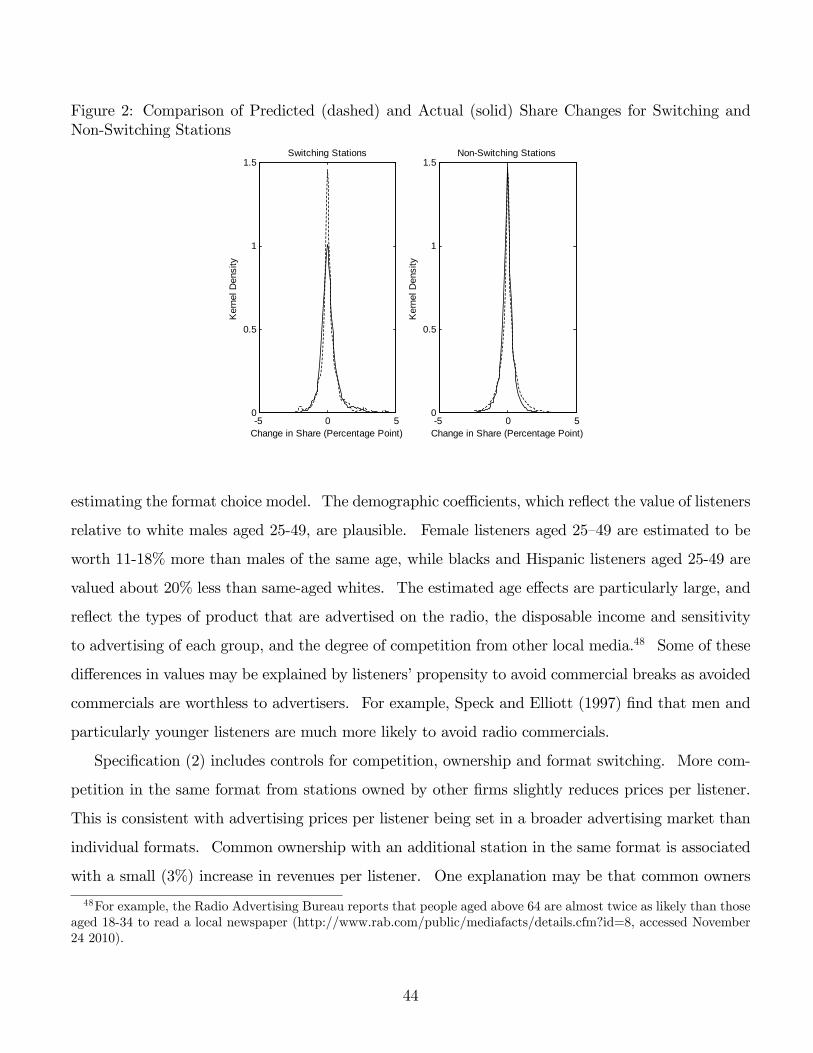
Figure 2: Comparison of Predicted (dashed) and Actual (solid) Share Changes for Switching andNon-Switching Stations

­5 0 50

0.5

1

1.5Switching Stations

Change in Share (Percentage Point)

Ker

nel D

ensi

ty

­5 0 50

0.5

1

1.5Non­Switching Stations

Change in Share (Percentage Point)

Ker

nel D

ensi

ty

estimating the format choice model. The demographic coe¢ cients, which re�ect the value of listeners

relative to white males aged 25-49, are plausible. Female listeners aged 25�49 are estimated to be

worth 11-18% more than males of the same age, while blacks and Hispanic listeners aged 25-49 are

valued about 20% less than same-aged whites. The estimated age e¤ects are particularly large, and

re�ect the types of product that are advertised on the radio, the disposable income and sensitivity

to advertising of each group, and the degree of competition from other local media.48 Some of these

di¤erences in values may be explained by listeners�propensity to avoid commercial breaks as avoided

commercials are worthless to advertisers. For example, Speck and Elliott (1997) �nd that men and

particularly younger listeners are much more likely to avoid radio commercials.

Speci�cation (2) includes controls for competition, ownership and format switching. More com-

petition in the same format from stations owned by other �rms slightly reduces prices per listener.

This is consistent with advertising prices per listener being set in a broader advertising market than

individual formats. Common ownership with an additional station in the same format is associated

with a small (3%) increase in revenues per listener. One explanation may be that common owners

48For example, the Radio Advertising Bureau reports that people aged above 64 are almost twice as likely than thoseaged 18-34 to read a local newspaper (http://www.rab.com/public/mediafacts/details.cfm?id=8, accessed November24 2010).

44

Table 7: Parameter Estimates for the Revenue Function(1) (2) (3)

DEMOGRAPHICSFemale 0.1709 0.1794 0.1154

(0.0852) (0.0900) (0.0902)Age 12-24 -0.7582 -0.6787 -0.6533

(0.1962) (0.2100) (0.2091)Age 50+ -0.6022 -0.5825 -0.5288

(0.0953) (0.0994) (0.1022)Black -0.1913 -0.2118 -0.2020

(0.0272) (0.0297) (0.0287)Hispanic -0.1779 -0.1970 -0.1661

(0.0174) (0.0182) (0.0192)STATION CHARACTERISTICS AND COMPETITIONNumber of stations with same owner in format - 0.0293 0.0271

(0.0065) (0.0066)Number of other stations in format - -0.0025 -0.0005

(0.0020) (0.0020)Format switch in previous quarter - -0.1247 -0.0973

(0.0431) (0.0441)

Non-linear market share e¤ect - - 2.6846(Station market share - market average share) (0.3717)

R2 (compared to a model with only market-year 0.2165 0.2215 0.2306�xed e¤ects)

Note: 4,484 annual station observations. Market-year coe¢ cients not reported. Robust standarderrors in parentheses corrected for imprecision in the demand parameters.

45

can extract more money from advertisers by selling bundles of commercials on di¤erent stations,

reducing advertisers�transaction costs. Revenues per listener fall by 10% in the period following a

format switch, which may re�ect either fewer commercials being played or discounts being o¤ered

to advertisers while the station develops relationships with new advertisers. Speci�cation (3) also

allows for revenues per listener to increase in the station�s market share (measured relative to the

market average). Consistent with the literature on television advertising (Fisher et al. (1980)), the

positive coe¢ cient suggests that stations with higher shares (typically those of higher quality) get

higher revenues per listener. The size of the coe¢ cient implies that increasing a station�s market

share by one standard deviation from the market mean raises revenues per listener by 3.3%.

Although the reported R2s indicate that the model only explains some of the within-market

variation in station revenues, the model does do a reasonable job of predicting how station revenues

change over time. For example, for stations remaining in the same format, the correlation between

observed year-to-year changes in station revenues and those predicted by the model (conditional on

the observed changes in station audiences) is 0.40. For stations changing formats the correlation is

0.62.

6.3 Estimates of Repositioning Costs and Economies of Scope

Repositioning costs and economies of scope are estimated using the dynamic model. Table 8 shows

the coe¢ cient estimates from four speci�cations. The �rst one only includes repositioning costs,

and the next two add local and national economies of scope. The fourth speci�cation repeats the

third speci�cation, increasing the number of simulated draws for moves by other �rms in the same

market from 500 to 1000, and the number of draws by �rms in other markets with the same corporate

owner from 100 to 200. This provides a robustness check on whether the accuracy of the integration

procedure has signi�cant e¤ects on the results. Standard errors are calculated using a non-parametric

block bootstrap (50 repetitions, 25 in the case of speci�cation 4) where markets are re-sampled (with

the same resampling scheme used for each speci�cation).49 The �nal row of the table reports the R2

49Because of cross-market economies of scope, markets cannot be dropped entirely, and the set of states used toapproximate the value function remains the set of observed states in all of the sample markets. Instead, the bootstrap isapplied by reweighting observations from di¤erent markets when performing the maximum pseudo-likelihood procedurefor each NPL iteration. The standard errors do not account for error in the listener demand and revenue models.However, the coe¢ cient estimates in these models are precise, so accounting for this would likely have small e¤ects onthe results.

46

from the regression which approximates the value function at the estimated parameters and choice

probabilities. In all four speci�cations the R2 is above 0.99. All of the speci�cations also achieved

convergence of the choice probabilities, so that no element of P i and P 0 di¤ers by more than 1e� 5

(see point 7 of the estimation methodology in Section 5.4).

The signs of the coe¢ cients are sensible. For example, it should be more expensive to move

stations with higher existing revenues and less expensive to move stations that are currently o¤-air

or which have recently switched formats if one of the main costs of repositioning is the loss of the

goodwill of loyal listeners and advertisers. The negative coe¢ cient on market size for the cost of a

switch to an active format re�ects the fact that relatively small stations in large markets are more

likely to change formats than larger stations in smaller markets, even if, because of the di¤erence in

market size, their revenues are larger. This may re�ect the fact that the leading �rm in a market

format has the most goodwill to lose if it switches formats. Switching to being o¤-air is estimated

to be more expensive than switching to an active format, which re�ects how few stations go o¤-air

in the data. There is also evidence of statistically signi�cant local and national economies of scope.

Table 14 shows the average size of repositioning costs and local economies of scope implied by the

coe¢ cients from speci�cation (3) for three sets of markets with di¤erent populations. The �rst line of

the table lists the average per-period revenues of stations in each market group based on their BIAfn

estimated revenues in Fall 2004.50 In the largest markets, average repositioning costs are estimated

to be equal to one period�s revenues for the average station, while in smaller markets estimated

repositioning costs could be equal to 2 or 3 periods of revenue. Higher relative repositioning costs in

smaller markets, which tend to reduce the amount of switching, are partly o¤set by the higher relative

variance of the payo¤ shocks, which, for given repositioning costs, tends to increase the amount of

switching. Local economies of scope are estimated to be quite substantial: adding one more station

to a format where a �rm already owns a station can reduce �xed costs by around 20% of average

station revenues. The implied total value of local economies of scope (for the sample markets) in

Fall 2004 is $236 million. Of course, this �gure does not include economies of scope that can be

realized by operating �rms in the same market but not in the same format (e.g., reduced transmitter

maintenance costs). As a comparison, the estimates imply that the realized value of cross-market

economies of scope in Fall 2004 was $63 million.

50The stations which have no BIAfn revenue estimates are ignored.

47

Table8:ParameterEstimatesfrom

theDynamicModel

(1)

(2)

(3)

(4)

Speci�cation

Repositioning

(1)+Local

(2)+Cross-

(3)+more

CostsOnly

Econ.of

MarketEcon

draws

Scope

ofScope

REPOSITIONINGCOSTS:

COSTSOFMOVETOACTIVEFORMAT($M.)

FixedComponent

1.341

1.259

1.242

1.251

(0.376)

(0.343)

(0.362)

(0.340)

*Pre-MoveRevenueofMovingStation(mean0.92,std.dev.1.46)

0.909

0.876

0.909

0.896

(0.236)

(0.224)

(0.241)

(0.227)

*MarketSizeMeasure(mean0.09,std.dev0.10)

-0.307

-0.490

-0.552

-0.540

(0.186)

(0.274)

(0.390)

(0.383)

*FormatSwitchinPreviousPeriod(indicator)

-0.642

-0.644

-0.658

-0.653

(0.154)

(0.149)

(0.160)

(0.154)

*FormatSwitch*Pre-MoveRevenueofMovingStation

-0.486

-0.469

-0.474

-0.480

(0.193)

(0.150)

(0.168)

(0.162)

*RecentFormatSwitch*MarketSizeMeasure

-2.915

-2.396

-2.345

-2.363

(1.939)

(1.836)

(1.902)

(1.864)

ADDITIONALCOSTSOFMOVINGTOACTIVEFROMDARK($M.)

FixedComponent

-0.741

-0.693

-0.642

-0.660

(0.350)

(0.320)

(0.321)

(0.303)

*MarketSizeMeasure

11.873

13.008

12.616

12.720

(1.890)

(2.355)

(2.460)

(2.609)

48

Table13:ParameterEstimatesfrom

theDynamicModelcont.

(1)

(2)

(3)

(4)

COSTSOFMOVEFROMACTIVETODARK($M.)

FixedComponent

1.515

1.434

1.341

1.354

(0.683)(0.562)(0.482)(0.434)

*Pre-MoveRevenueofMovingStation

5.149

6.186

5.690

5.777

(5.245)(4.973)(5.155)(4.902)

*MarketSizeMeasure

-1.327

-1.642

-1.652

-1.640

(1.442)(1.066)(1.443)(1.374)

LOCALECONOMIESOFSCOPE:REDUCTIONINFIXED

WHENADDONEMORESTATIONTOFORMAT($M.)

FixedComponent

-0.076

0.042

0.048

(0.025)(0.020)(0.020)

*MarketSizeMeasure

-2.851

2.813

2.811

(0.618)(0.405)(0.378)

CROSSMARKETECONOMIESOFSCOPE

0.013

0.014

(seespeci�cationinSection3)

(0.005)(0.004)

--

STANDARDDEVIATIONOF"s

Constant

0.321

0.306

0.303

0.303

(0.120)(0.108)(0.103)(0.110)

LocalFirmRevenuePriortoSwitch

0.038

0.040

0.041

0.040

(0.004)(0.003)(0.005)(0.004)

R2forparametricapproximation(atestimatedparameters)

0.9918

0.9911

0.9906

0.9907

6,046localmarket�rmobservationsusedtocalculatedpseudo-likelihood.

Standarderrorsinparenthesescalculatedusinganon-parametricbootstrap.

49

Table 14: Average Values of Repositioning Costs and Economies of Scope By Market SizeMarket Size Group Small Mid Large

Population < 0.25 mil. 0.25 - 1 mil. � 1 mil.Average (Half-Year) Station Revenue ($m.) 0.45 0.81 2.59

Implied Average Repositioning Cost for A Switch 1.45 1.66 2.59Between Active Formats ($m.) (0.42) (0.49) (0.55)Average Incremental Value of Local 0.090 0.181 0.570Economy of Scope ($m.) (0.029) (0.043) (0.065)Total Local Economies of Scope in 15.33 61.71 159.59Fall 2004 ($m.) (4.71) (14.55) (19.64)Average Std Deviation of Payo¤ Shocks ($m.) 0.333 0.373 0.512

(0.125) (0.131) (0.145)

Model Fit.

Table 15 contains statistics that summarize how well the estimated model (speci�cation (3)) does

at matching format switching patterns in the data at the station (not �rm) level. The �rst four

rows compare the mean probabilities of remaining in the same format for di¤erent groups of stations

depending on their ownership, and shows that the model �ts well for each group. The next two rows

show that the model also does a reasonable job of predicting which stations move in the sense that the

predicted probability of remaining in the same format is signi�cantly lower for these stations (even

though it is above 0.9 on average). For moving stations, the predicted probabilities of the chosen

moves are also signi�cantly higher than those for moves that are not chosen, which is consistent with

the estimated listener demand and revenue models capturing quite accurately how a �rm expects its

stations�market shares and revenues to change when a station changes formats.

7 Counterfactual: The E¤ect of the Proposed Performance

Rights Act on Format Choices

I now examine how the introduction of a performance rights fees on contemporary music stations,

implemented as a % �tax�on revenues, would a¤ect format choices. I de�ne AC/CHR/Rock, Country

and Urban as contemporary music formats. I also solve the model under di¤erent assumptions on

station ownership, repositioning costs and heterogeneity in listener tastes in order to understand how

these industry characteristics a¤ect the impact of a tax. It is particularly useful to understand the

50

Table 15: Fit of the Dynamic ModelEstimated Model Data

Mean probability of remaining in same formatall stations 0.971 0.967independent stations 0.975 0.969stations owned by local �rms with 2 or 3 stations 0.980 0.976stations owned by local �rms with more than 4 stations 0.965 0.968

Mean probability of remaining in same format for stations that do move 0.913 -

Mean probability of remaining in same format for stations that do not move 0.972 -

Mean probability of chosen move for stations that move 0.037 -

Mean probability of not chosen moves for stations that move 0.010 -

e¤ects of multi-station ownership and taste heterogeneity as these factors might be excluded from

simpler models that could be solved without parametric approximation.

7.1 Solving the Model for the Counterfactual

Given the point estimates of the structural parameters estimated above (column 3 of Table 8), solving

the model for the counterfactual involves two steps.

1. �nd a new set of parameters �CF that approximate the equilibrium value function when the tax

is imposed. This involves solving the model holding the structural parameters (e.g., listener

demand and repositioning costs) �xed, but rescaling the (post-tax) revenues of contemporary

music stations. The set of states chosen is the same set of states used for estimating the model

(i.e., the observed states in all periods), which the Monte Carlo experiments in the Appendix

suggest is appropriate;

2. forward simulation. I analyze how the industry evolves over 30 periods after the introduction

of the tax. For the �rst period, the equilibrium choice probabilities are found in step 1, and

these are used, together with the processes for demographics and station quality, to simulate

the model forward to the second period. For the new state it is necessary to �nd equilibrium

choice probabilities given �CF . The steps for solving the model are therefore repeated (i.e., a

51

single agent model is solved �rst to determine the states used in integration, followed by the

game) to give the equilibrium choice probabilities, except that �CF is held �xed.51 These new

choice probabilities are used to simulate the model forward to the third period, and the process

is then repeated.

I start the simulations from Fall 2004. For each tax level I simulate the model forward 25 times,

and the numbers reported below are averages and standard deviations across these 25 simulations.52

Equilibrium Selection.

It is well known that dynamic games can have multiple equilibria, and this presents a potential

challenge for performing counterfactuals because even if the equilibrium played in the data is correctly

identi�ed it is impossible to know which equilibrium will be played when fees are imposed. The

complexity of the current model makes it extremely di¢ cult to enumerate all of the equilibria that the

game may have. The approach used to solve for both the counterfactual �CF and to �nd the choice

probabilities during forward simulation is to �rst solve a (�ctitious) single agent model (where each

�rm assumes that other �rms will not move their stations), which should have a unique equilibrium,

and then to use the associated parameters and choice probabilities as starting points for best response

iterations to �nd the parameters and choice probabilities associated with the equilibrium of the full

game.

A couple of pieces of evidence suggests that this procedure �nds equilibria that are at least

plausible. First, the equilibrium choice probabilities and � parameters vary quite smoothly in the

assumed tax rate, i.e., when the tax rate is changed by a small amount, the procedure identi�es an

equilibrium that is close by in probability space. It seems plausible that this type of equilibrium

would be played when the tax rate is changed slightly.53 Second, it is possible to compare the

equilibria found by this method with those that are found from iterating best responses from starting

51As this creates a signi�cant computational burden the number of possible moves for other stations in the samemarket that are sampled for the next period to perform the integrations is 100 rather than 500. However, I checkedthat for a 10% tax the evolution of the industry was almost identical when 250 or 500 simulations were used.52Note, I use the point estimates from speci�cation (3) in Table 8 in all of the simulations, so the standard deviations

do not re�ect the lack of precision in some of the parameter estimates.53The equilibria of dynamic games are typically isolated (see, for example, Dorazelski and Escobar (2010)) so one

would not expect there to be many nearby equilibria when the tax rate is changed by a small amount. Of course,proximity in probability space is not the only criterion that one might use. Aguirregabiria (2009) presents a methodfor �nding equilibria based on Taylor expansions, under the assumption that the unobserved equilibrium selectionmechanism is smooth in the structural parameters, which would include the tax rate. He presents an exampleshowing that this approach, which also seems attractive, may not select the equilibrium that is nearest to the originalequilibrium in probability space.

52

Table 16: Evolution of the Number of Music Stations Under Di¤erent Performance Rights FeesFees, As a % of Revenues

0% 5% 10% 15% 20%Period prior to introduction 1,401 1,401 1,401 1,401 1,401(Fall 2004)+1 period 1,409 1,403 1,397 1,387 1,379

(4.7) (5.1) (5.3) (6.2) (7.1)+5 periods 1,418 1,392 1,370 1,351 1,309

(13.1) (11.1) (13.1) (13.4) (14.7)+10 periods 1,416 1,373 1,330 1,287 1,219

(16.1) (14.8) (16.1) (19.1) (21.5)+15 periods 1,413 1,357 1,297 1,234 1,157

(16.2) (16.1) (18.8) (20.5) (20.4)+20 periods 1,411 1,343 1,272 1,191 1,096

(17.2) (21.4) (18.0) (21.6) (24.2)+25 periods 1,413 1,337 1,260 1,170 1,070

(14.7) (21.8) (20.1) (22.5) (23.9)+30 periods 1,415 1,336 1,258 1,160 1,053

(16.8) (21.0) (25.0) (22.0) (20.7)

Standard deviations across 25 simulations in parentheses.

points that are not those of the single-agent model. For fees equal to 0%, 5% and 10% of revenues,

I re-started the best response procedure for �nding �CF and the initial period equilibrium choice

probabilities from several di¤erent starting points and found that they converged to values that are,

for practical purposes, identical to those considered here.

7.2 The E¤ects of Performance Fees on Market Structure

Table 16 shows how the number of contemporary music formats in the sample markets is predicted

to change following the introduction of di¤erent levels of fees. With no fees the number of music

stations is predicted to increase in the �rst few periods and then remain fairly constant. As one

would expect, larger fees have greater impacts on the number of music stations. For example, a 5%

fee is predicted to reduce the number of contemporary music stations by only 6% over 15 years (30

periods) relative to the case with no fees. On the other hand, a 20% fee, which is towards the upper

end of what might be charged, would reduce the number of music stations by 25%. The number

of stations is predicted to fall in all three music formats with slightly larger falls in AC/CHR/Rock

53

(30% with a 20% fee) than Country or Urban (16% and 18% respectively), while all three non-music

formats would gain stations. News/Talk would experience the largest gains, which is consistent with

News/Talk stations tending to appeal to similar demographics (white, middle-aged) as AC and Rock

stations. The number of Dark (o¤-air) stations is predicted to increase only slightly (10 stations

over 30 periods or 0.1 per market). The table also shows that the format structure tends to evolve

relatively slowly: for example, with a 10% fee the number of music stations falls (relative to the

no fee case) at a rate of 8.6 stations per period in the �rst 5 years54, 5.3 stations per period in the

next 5 years and 1.9 stations per period in the �nal 5 years of the simulations. Slow adjustment

will be partly driven by the fact that �rms will tend to wait for a favorable " draw for a switch to

a non-music format before moving, as this will tend to o¤set the repositioning cost. I investigate

other factors that may a¤ect adjustment below.

The listener demand estimates indicate that many consumers will have strong preferences for

stations in a particular music format, either because of demographics or because of unobserved taste

heterogeneity, and these listeners will tend to substitute to the remaining stations in a format if

their preferred station switches to non-music programming. The �rst two columns of Table 17 show

how the average (unweighted across markets) contemporary music audience and the number of music

stations would change with a 10% tax (relative to the case of no tax), where, to make comparisons as

easy as possible Fall 2004 levels have been indexed to be equal to 1. Over 15 years, music audiences

fall by proportionally less than the number of music stations, consistent with this type of substitution.

On the other hand, in the �rst few periods after the introduction of fees, music audiences fall more

quickly than the number of stations, because higher quality stations are more likely to move quickly,

even though, with no fees, these stations are less likely to switch. I consider one possible explanation

for this pattern below.

7.3 The E¤ects of Taste Heterogeneity, Repositioning Costs and Own-

ership on Industry Transition

I now consider how the level of repositioning costs, listeners�heterogeneous tastes for di¤erent formats

and multi-station ownership a¤ect how the industry responds to the introduction of a 10% tax. The

54A rate of 8.6 stations per period over 102 markets implies that the average market would lose a music stationevery 6 years.

54

Table 17: Evolution of the Number of Music Stations and Music Audiences under a 10% Fees forDi¤erent Assumptions on the Structural Parameters Relative to Evolution with No Fees (Fall 2004indexed to 1)

True Parameters Less Taste Lower Repositioning Independent StationHeterogeneity Costs Ownership

Column (1) (2) (3) (4) (5) (6) (7) (8)Stations Audience Stations Audiences Stations Audience Stations Audience

Fall 2004 1 1 1 1 1 1 1 1

+1 period 0.991 0.985 0.981 0.977 0.982 0.975 0.994 0.989(0.004) (0.009) (0.006) (0.011) (0.008) (0.011) (0.007) (0.008)

+2 periods 0.983 0.970 0.959 0.951 0.963 0.951 0.989 0.983(0.007) (0.012) (0.009) (0.014) (0.012) (0.013) (0.010) (0.010)

+5 periods 0.966 0.961 0.926 0.921 0.942 0.942 0.978 0.974(0.010) (0.013) (0.013) (0.019) (0.015) (0.014) (0.012) (0.013)

+10 periods 0.939 0.953 0.858 0.873 0.907 0.932 0.954 0.963(0.011) (0.012) (0.014) (0.020) (0.019) (0.015) (0.014) (0.012)

+15 periods 0.918 0.947 0.801 0.862 0.891 0.931 0.932 0.955(0.013) (0.011) (0.016) (0.018) (0.020) (0.014) (0.015) (0.016)

+20 periods 0.901 0.944 0.785 0.847 0.886 0.930 0.910 0.948(0.012) (0.010) (0.017) (0.016) (0.018) (0.013) (0.016) (0.015)

+25 periods 0.892 0.942 0.783 0.847 0.884 0.932 0.899 0.944(0.013) (0.009) (0.016) (0.017) (0.015) (0.014) (0.018) (0.012)

+30 periods 0.890 0.941 0.784 0.844 0.882 0.930 0.894 0.942(0.012) (0.012) (0.018) (0.015) (0.015) (0.013) (0.016) (0.013)

Standard deviations across 25 simulations in parentheses. Audience measured based on averagecombined market share of music stations across markets.

55

taste heterogeneity and ownership comparisons are particularly interesting as these features might

be ignored if one made the model simple enough to solve and estimate without using parametric

approximation. The results also provide some suggestive insights about what might happen in other

settings.55

Taste Heterogeneity. The estimates of listener demand imply that many listeners have strong

preferences for particular formats, which implies that when one station switches from a music format

the audience of the remaining stations will increase. To understand how the extent of taste hetero-

geneity a¤ects repositioning I resolve the model (for no tax and a 10% tax rate) assuming that �

and all of the demographic taste parameters are equal to half of their estimated values.56 Columns

(3) and (4) of Table 17 shows how the industry would adjust given these hypothetical parameters.57

As one might expect, more stations move when format preferences are weaker, and the change in

audiences is also relatively large. The adjustment is also predicted to take place more quickly. This

may be explained by music stations having less to gain if they wait and one of their competitors

moves.

Repositioning Costs. Repositioning costs make it more expensive for music stations to switch

to non-music formats. Columns (5) and (6) of Table 17 shows the adjustment of the industry when

the parameters determining repositioning costs between active formats are reduced by 25% (the taste

parameters take their estimated values). The level of repositioning costs only has a small e¤ect on

the number of music stations in the long-run. This is sensible because the attractiveness of each

format is ultimately determined by listener and advertiser preferences and the level of the tax, and

the existence of " payo¤ shocks means that stations will change their formats eventually for any level

of repositioning costs. However, lower repositioning costs make the adjustment happen more quickly

and also make the adjustment less expensive: with the original parameters, the additional switches

from music to non-music formats when a 10% tax is introduced cost approximately $290 million (no

discounting). When repositioning costs are 25% lower, the additional switches cost $233 million

55For example, consider taste heterogeneity. Suppose that a tax is imposed on sugar-sweetened soft drinks (Wang(2010)). If no consumers have a strong preference for sugar-sweetened drinks then, as long as these drinks are notmuch cheaper to produce, we would expect future innovation to be concentrated in non-sugar-sweetened products.56This simulation is performed with values for the linear demand parameters, �st and �st which would be estimated

if the random coe¢ cients had these hypothetical values. However, in order to isolate the e¤ects of changing F I usethe same values of the revenue function, repositioning cost and economies of scope parameters that were estimatedusing the full model.57As before, the table shows the di¤erence between what happens with a 0% tax and a 10% tax. With no fee the

model predicts a small �ow of stations into music formats.

56

(20% lower).58

Multi-Station Ownership. Taste heterogeneity and repositioning costs a¤ect the industry�s

adjustment in ways that are fairly predictable. The likely e¤ects of multi-station ownership are less

clear. I re-solve the model assuming that all stations are independent, which has three e¤ects on

the model. First, there are no economies of scope. Second, multi-station �rms no longer coordinate

the location of their stations, taking into account, for example, audience cannibalization. Third,

given my simplifying assumption that a local �rm can only move one station at a time, the number

of format switches that can happen each period increases, which could mechanically speed up the

industry�s adjustment. However, as can be seen in columns (7) and (8) of Table 17, the adjustment is

predicted to take place more slowly with independent �rms. This suggests that the coordinating role

of multi-station owners speeds the industry�s transition when the tax is introduced. In particular,

independent music stations may delay moving in the hope that one of their competitors will pay the

repositioning cost and restore the pro�tability of the remaining stations. This could slow the exit of

stations from music formats, as can happen when a �war of attrition�determines which �rm exits a

declining market (Maynard Smith (1974), Tirole (1988), p. 311-4). In contrast, the owner of two or

more stations in the same music format may want to move one of its stations more quickly because

it internalizes how this will increase the pro�tability of its remaining stations.

Ownership also provides a potential explanation for why higher quality stations tend to move more

quickly when the tax is introduced because higher quality stations tend to be owned by multi-station

local �rms. To investigate further, I calculate how the tax changes the probability that each music

station switches to a non-music format when it is �rst introduced (to provide more observations I do

this for all states observed in the data, not just those for Fall 2004) using the observed ownership

structure. The change in probability is regressed on a constant, current format dummies, estimated

station quality (�) from the listener demand model, dummies for the number of stations that the

station�s owner owns in the market (this a¤ects the number of options a �rm has and mechanically

reduces the probability of a particular station moving), and a count of the number of stations that

the station�s owner has in that format, plus the interaction of � and this count variable. If ownership

e¤ects are important then we would expect the coe¢ cients on the �nal two variables to be signi�cant,

58The number of extra switches when a fee is imposed is greater than the net �ow of stations into non-music formatsmight suggest. This partly re�ects the fact that once a station switches it is more likely to switch again the followingperiod, and the fact that more than one station might make a similar move in a particular period, creating an incentivefor additional moves.

57

Table 18: Regression of Change in First Period Probabilities of Moving to a Non-Music for eachStation with a 10% Tax

(1) (2)� (station quality) 0.0058 0.0072

(0.0007) (0 0009)Number of owned stations in format 0.0003 -0.0006

(0.0021) (0.0021)Number of owned stations in format * � 0.0011 0 0008

(0.0003) (0.0003)

Controls Format Dummies Dummies for the NumberDummies for the Number of Local Stations Ownedof Local Stations Owned

Number of observations 8,505 8,505

Market-Format-Period Fixed E¤ects No Yes

Adjusted R2 0.055 0.462(includes �xed e¤ects)

Standard errors in parentheses.

whereas if there is only a station quality e¤ect only the �rst variable should be signi�cant. The

�rst column of Table 18 reports the results of this speci�cation, while the second column shows the

results when market-format-period �xed e¤ects are included to control for any factors that a¤ect all

stations in a particular local market-format.

The coe¢ cients are similar in both speci�cations, and they indicate that fees make it more likely

that higher quality stations will move, but that this is particularly true for higher quality stations

owned by �rms with several music stations in the same format. The � coe¢ cient implies that a

one unit increase in � (approximately equal to one within-market-format standard deviation) raises

the probability of a station moving to a non-music format by 0.006-0.007, relative to a mean station

probability of moving (to a non-music format) before the tax of 0.013 and after the tax of 0.017.

This is likely to be because the loss created by the tax is larger relative to the repositioning cost for

higher quality stations that can attract more listeners in any format. The coe¢ cients in the �rst

column imply that the increase in probability would be 0.01, rather than 0.006, for a station with

two sister stations in the same music format. This additional e¤ect suggests a coordinating role of

multi-station ownership.

58

8 Conclusion

This article has analyzed the likely e¤ects of performance rights fees on format choices in the broadcast

radio industry. Currently broadcast radio stations do not have to compensate performers or record

labels when they play their music, but proposed legislation would introduce possibly quite substantial

fees for performance rights. This setting provides a close to ideal environment for think about the

general e¤ects of policies that favor particular types of product in a di¤erentiated product industry,

because the set of available products (stations) is well-de�ned and, even in the absence of fees, quite

a lot of product repositioning is observed. My results predict that if a fee equal to 10% of station

revenues was levied on contemporary music stations, the number of music stations would fall by 11%

in a 15 year period, with the adjustment taking place relatively slowly. By resolving the model for

di¤erent parameters, I show how listeners�heterogeneous tastes for di¤erent formats, repositioning

costs and multi-station ownership a¤ect the adjustment. The number of music stations and the

number of people listening to music radio decline by more when listeners�have weaker preferences for

particular types of programming, while the level of repositioning costs and multi-station ownership

primarily a¤ect the speed with which the industry adjusts to the tax.

The article has also made a methodological contribution by illustrating how parametric approxi-

mations to the value function can be used to estimate and re-solve dynamic games in a setting with

a very rich state space, which is necessary to model industries with many asymmetric �rms and rich

horizontal and vertical product di¤erentiation. The evidence of Monte Carlo experiments, as well

as the plausible empirical results, suggest that the method works well in my setting, and that it

could also be applied in other industries with similar characteristics. My experience suggests that

some features of the radio industry help the approach to work well here. In particular, the estimated

models of listener demand and revenues provide predictions of a station�s revenues in di¤erent format

con�gurations, and a small number of variables that measure a �rm�s current revenues and its oppor-

tunities to increase its revenues by moving stations to di¤erent formats explain a lot of the variation

in �rm values, which would otherwise have to be captured by very rich functions that interact many

of the state variables in a highly non-linear way. The predictive power of the variables based on

current station attributes is increased by the fact that market demographics and station qualities

change quite slowly, and the rate of station format switching is quite low. This latter problem may

also help to relieve problems associated with multiple equilibria, where �rms would make di¤erent

59

equilibrium choices based on their beliefs about what other �rms will choose. However, it will be

interesting and important to test the accuracy of the model�s predictions if and when performance

fees are eventually introduced.

60

References

[1] Alho, Juha M. and Bruce D. Spencer (2005), Statistical Demography and Forecasting, New York:

Springer

[2] Aguirregabiria, Victor (2009), �A Method for Implementing Counterfactual Experiments in

Models with Multiple Equilibria�, mimeo, University of Toronto

[3] Aguirregabiria, Victor and Chun-Yu Ho (2009), �A Dynamic Oligopoly Game of the US Airline

Industry: Estimation and Policy Experiments�, mimeo, University of Toronto

[4] Aguirregabiria, Victor and Pedro Mira (2007), �Sequential Estimation of Dynamic Discrete

Games�, Econometrica, 75(1), 1-53

[5] Aguirregabiria, Victor, Pedro Mira and Hernan Roman (2007), �An Estimable Dynamic Model

of Entry, Exit, and Growth in Oligopoly Retail Markets�, American Economic Review, 97 (2)

449-454

[6] Aguirregabiria, Victor and Aviv Nevo (2010), �Recent Developments in Empirical Dynamic

Models of Demand and Competition in Oligopoly Markets�, mimeo, University of Toronto

[7] Albarran, Alan B. and W. Lawrence Patrick (2005), �Assessing Radio Station Value: A Review

of Academic Literature and Analysis of Contemporary Industry Models�, Journal of Radio &

Audio Media, 12(1), 3�13

[8] Arbitron Company (2002), Arbitron Radio Market Report Reference Guide, New York, NY:

Arbitron Company

[9] Arbitron Company, Radio Today, various years, New York, NY: Arbitron Company

[10] Arcidiacono, Peter and Robert Miller (2010), �CCP Estimation of Dynamic Discrete Choice

Models with Unobserved Heterogeneity�, mimeo, Duke University

[11] Bajari, Patrick, Lanier Benkard and Jonathan Levin (2007), �Estimating Dynamic Models of

Imperfect Competition�, Econometrica, 75(5), 1331-1370

61

[12] Benitez-Silva, Hugo, George Hall, Gunter Hitsch, Giorgio Pauletto and John Rust (2000): �A

Comparison of Discrete and Parametric Approximation Methods for Continuous-State Dynamic

Programming Problems,�mimeo, Yale University

[13] Benkard, C. Lanier, Aaron Bodoh-Creed and John Lazarev (2010), �Simulating the Dynamic

E¤ects of Horizontal Mergers: U.S. Airlines�, mimeo, Yale University

[14] Beresteanu, Arie, Paul B. Ellickson and Sanjog Misra (2010), �The Dynamics of Retail

Oligopoly�, mimeo, University of Rochester

[15] Berry, Steven T. (1994), �Estimating Discrete-Choice Models of Product Di¤erentiation�, RAND

Journal of Economics, 25(2), 242-262

[16] Berry, Steven T., James Levinsohn and Ariel Pakes (1993), �Applications and Limitations of

Some Recent Advances in Empirical Industrial Organization: Price Indexes and the Analysis of

Environmental Change�, American Economic Review, 83(2), 240-246

[17] Berry, Steven T., James Levinsohn and Ariel Pakes (1995), �Automobile Prices in Market Equi-

librium�, Econometrica, 63(4), 841-890

[18] Berry, Steven T. and Joel Waldfogel (1999), �Free Entry and Social Ine¢ ciency in Radio Broad-

casting�, RAND Journal of Economics, 30(2), 397-420

[19] Berry, Steven T. and Joel Waldfogel (2001), �Do Mergers Increase Product Variety? Evidence

from Radio Broadcasting�, Quarterly Journal of Economics, 116(3), 1009-1025

[20] Bertsekas, Dimitri (2010), �Approximate Policy Iteration: A Survey and Some New Methods�,

Laboratory for Information and Decision Systems Report No. 2833, MIT

[21] Bertsekas, Dimitri and Huizhen Yu (2007), �Solution of Large Systems of Equations Using Ap-

proximate Dynamic Programming Methods�, Laboratory for Information and Decision Systems

Report No. 2754, MIT

[22] Bertsekas, Dimitri and Sergey Io¤e (1996), �Temporal Di¤erences-Based Policy Iteration and

Applications in Neuro-Dynamic ProgrammingSolution of Large Systems of Equations Using Ap-

62

proximate Dynamic Programming Methods�, Laboratory for Information and Decision Systems

Report No. 2349, MIT

[23] BIA Financial Network, Inc. (2006), Media Access Pro User�s Manual, version 3.0, Chantilly,

VA: BIA Financial Network, Inc.

[24] Collard-Wexler, Allan (2010), �Demand Fluctuations in the Ready-Mix Concrete Industry�,

mimeo, New York University

[25] Draganaska, Michaela, Michael Mazzeo and Katja Seim (2009), �Beyond Plain Vanilla: Modeling

Joint Pricing and Product Assortment Choices�, Quantitative Marketing and Economics, 7(2),

105-46

[26] Doraszelski, Ulrich and Mark Satterthwaite (2010), �Computable Markov-Perfect Industry Dy-

namics�, RAND Journal of Economics, 41(2), 215-43

[27] Doraszelski, Ulrich and Juan Escobar (2010), �A Theory of Regular Markov Perfect Equilibria

in Dynamic Stochastic Games: Genericity, Stability, and Puri�cation�, Theoretical Economics,

5(3), 369-402

[28] Dube, Jean-Pierre H. and Jeremy T. Fox and Che-Lin Su (2009), �Improving the Numerical

Performance of BLP Static and Dynamic Discrete Choice Random Coe¢ cients Demand Esti-

mation�, National Bureau of Economic Research Working Paper No. 14991

[29] Duncan, James H., Duncan�s American Radio, issues from Spring 1996 to Spring 2001

[30] Ericson, Richard and Ariel Pakes (1995), �Markov Perfect Industry Dynamics: A Framework

for Empirical Work�, Review of Economic Studies, 62(1), 53-82

[31] Fan, Ying (2010), �Ownership Consolidation and Product Quality: A Study of the U.S. Daily

Newspaper Market�, mimeo, University of Michigan

[32] Federal Communications Commission (2001), Review of the Radio Industry, 2001, Mass Media

Bureau Policy and Rules Division, Washington DC: Federal Communications Commission

[33] Fisher, Franklin M., John F. McGowan and David S. Evans (1980), �The Audience-Revenue

Relationship for Local Television Stations�, Bell Journal of Economics, 11(2), 694-708

63

[34] Hendel, Igal and Aviv Nevo (2006), �Measuring the Implications of Sales and Consumer Inven-

tory Behavior�, Econometrica, 74(6), 1637-1673

[35] Hitsch, Gunter J. (2006), �An Empirical Model of Optimal Dynamic Product Launch and Exit

Under Demand Uncertainty�, Marketing Science, 25(1), 25-50

[36] Ho, Katherine (2006), �The Welfare E¤ects of Restricted Hospital Choice in the US Medical

Market�, Journal of Applied Econometrics, 21, 1039-1079

[37] Hotz, V. Joseph and Robert A. Miller (1993), �Conditional Choice Probabilities and the Esti-

mation of Dynamic Models�, Review of Economic Studies, 60(3), 497-529

[38] Hotz, V. Joseph, Robert A. Miller, Seth Sanders and Je¤rey Smith (1994), �A Simulation

Estimator for Dynamic Models of Discrete Choice�, Review of Economic Studies, 61(2), 265-89

[39] Gowrisankaran, Gautam (1999), �E¢ cienct Representation of State Spaces for Some Dynamic

Models�, Journal of Economic Dynamics and Control, 23(8), 1077-1098

[40] Jenkins, Mark, Paul Liu, Rosa L. Matzkin and Daniel L. McFadden (2004), �The Browser War:

Econometric Analysis of Markov Perfect Equilibrium in Markets with Network E¤ects�, mimeo,

Stanford University

[41] Jeziorski, Przemyslaw (2009), �Dynamic Determinants of Mergers and Product Characteristics

in the Radio Industry�, mimeo, Johns Hopkins University

[42] Jeziorski, Przemyslaw (2010), �Merger enforcement in two-sided markets�, mimeo, Johns Hop-

kins University

[43] Judd, Kenneth L. (1998), Numerical Methods in Economics, MIT Press: Cambridge, MA

[44] Kasahara, Hiroyuki and Katsumi Shimotsu (2009), �Sequential Estimation of Structural Models

with a Fixed Point Constraint�, mimeo, University of Western Ontario

[45] Keane, Michael P. and Kenneth L. Wolpin (1994), �The Solution and Estimation of Discrete

Choice Dynamic Programming Models by Simulation and Interpolation: Monte Carlo Evidence�,

Review of Economics and Statistics, 76(4), 648-672

64

[46] Knittel, Christopher R. and Konstantinos Metaxoglou (2008), �Estimation of Random Coe¢ -

cient Demand Models: Challenges, Di¢ culties and Warnings�, National Bureau of Economic

Research Working Paper No. 14080

[47] Ma, Jun and Warren B. Powell (2009), �Convergence Proofs of Least Squares Policy Iteration

Algorithm for High-Dimensional In�nite Horizon Markov Decision Process Problems�, mimeo,

Princeton University

[48] Macieira, Joao, (2007), �Extending the frontier: A structural model of investment and techno-

logical competition in the supercomputer industry�, mimeo, Virginia Tech

[49] Maynard Smith, J. (1974), �The Theory of Games and the Evolution of Animal Contests�,

Journal of Theoretical Biology, 47, 209-221

[50] Mooney, Catherine Tyler (2010a), �Cost Sharing and Strategic Programming Choices in Broad-

cast Radio�, mimeo, University of Oklahoma

[51] Mooney, Catherine Tyler (2010b), �A Two-Sided Market Analysis of Radio Ownership Caps�,

mimeo, University of Oklahoma

[52] Nevo, Aviv (2001), �Measuring Market Power in the Ready-to-Eat Cereal Industry�, Economet-

rica, 69(2), 307-342.

[53] Nevo, Aviv (2000), �A Practioner�s Guide to Estimation of Random-Coe¢ cients Logit Models

of Demand�, Journal of Economics and Management Strategy, 9(4), 513-548

[54] Nevo, Aviv and Federico Rossi (2008), �An Approach for Extending Dynamic Models to Settings

with Multi-Product Firms�, Economic Letters, 100(1), 49-52

[55] O�Gorman, Catherine and Howard Smith (2008), � E¢ ciency Gain from Ownership Deregula-

tion: Estimates for the Radio Industry�, mimeo, University of Oxford

[56] Pakes, Ariel, Berry, Steven T. and Michael Ostrovsky (2007), �Simple Estimators for the Para-

meters of Discrete Dynamic Games (with Entry/Exit Examples)�, RAND Journal of Economics,

38(2), 373-399

65

[57] Pesendorfer, Martin and Philipp Schmidt-Dengler (2008), �Asymptotic Least Squares Estimators

for Dynamic Games�, Review of Economic Studies, 75(3), 901-928

[58] Petrin, Amil (2002), �Quantifying the Bene�ts of New Products: The Case of the Minivan�,

Journal of Political Economy, 110(4), 705-729

[59] Rust, John (2000), �Parametric Policy Iteration: An E¢ cient Algorithm for Solving Multidi-

mensional DP Problems?�, mimeo, Yale University

[60] Seim, Katja (2006), �An Empirical Model of Firm Entry with Endogenous Product-Type

Choices�, RAND Journal of Economics, 37(3), 619-640

[61] Speck, Paul S. and Michael T. Elliott (1997), �Predictors of Advertising Avoidance in Print and

Broadcast Media Predictors of Advertising Avoidance in Print and Broadcast Media�, Journal

of Advertising, 26(3), 61-76

[62] Su, Che-Lin and Kenneth L. Judd (2010), �Constrained Optimization Approaches to Estimation

of Structural Models�, mimeo, University of Chicago

[63] Sweeting, Andrew T. (2010), �The E¤ects of Mergers on Product Positioning: Evidence from

the Music Radio Industry�, RAND Journal of Economics, 41(2), 372-97

[64] Tirole, Jean (1988), The Theory of Industrial Organization, MIT Press: Cambridge, MA

[65] Wang, Emily (2010), �Estimating the Distributional Impact of Taxes on Storable Goods: A

Dynamic Demand Model with Random Coe¢ cients�, mimeo, Duke University

[66] United States Government Accountability O¢ ce, �The Proposed Performance Rights Act Would

Result in Additional Costs for Broadcast Radio Stations and Additional Revenue for Record

Companies, Musicians, and Performers�, GAO-10-826, August 2010

66

A Monte Carlo Experiments

In this section I present a set of Monte Carlo experiments using a simpli�ed version of the model

that can be solved exactly to test how well the methods that I use for solving and estimating the

model perform in practice.59

A.1 Simpli�ed Model

I consider a simpli�ed discrete state version of the model that captures several features of the full

model.60 I suppose that the researcher observes a set of 60 markets, that are independent because

I assume that there are no economies of scope across markets. Markets di¤er in demographics (size

and ethnic composition), format tastes (which would be caused by age and sex variation in the full

model), ownership structure and station qualities. The size of a market is drawn from U [0:5; 1:5]

(an interpretation would be millions of people) and it is treated as �xed. There are two ethnicities

of listeners, with the proportion of type 2 listeners taking on possible values [0.1,0.3,0.5,0.7], with

period-to-period transition probability matrix shown in Table 19. There are seven stations in each

Table 19: Demographic Transition Matrixtime t+ 1

0.1 0.3 0.5 0.7

0.1 0.8 0.2 0 0time 0.2 0.2 0.6 0.2 0t 0.5 0 0.2 0.6 0.2

0.7 0 0 0.2 0.8

market, owned by four �rms. There are 20 markets with each of the following ownership structures

[4,1,1,1], [3,2,1,1] and [2,2,2,1] where the numbers indicate the number of stations owned by each

�rm. Stations di¤er in two �xed quality dimensions. One component (�) has a common e¤ect across

formats (e.g., signal coverage) and is randomly drawn from U [�0:5; 0:5], while, with probability 0.25,59Benitez-Silva et al. (2000) provide several examples in economic models without strategic interactions. Hendel

and Nevo (2006) apply PPI to estimate a single-agent dynamic demand model for storable goods.60The features that are missing from the simpli�ed model are cross-market economies of scope, the existence of a

Dark format, permanent di¤erences in revenues per listener across markets and stochastic evolution of station qualities.In practice, the �rst two are unlikely to be important as my estimates indicate that national economies of scope arefairly small and the Dark format is rarely chosen. Permanent di¤erences in revenues per listener across markets maybe mimicked by permanent di¤erences in format tastes across markets which are included in the simpli�ed model.Station qualities are also fairly persistent, so treating them as �xed should not distort the results too much.

67

a station is classi�ed as AM (AMs = 1). AM stations have a relative advantage in format 2 (a talk

format).

A station can be in one of three active formats (no Dark format). A station�s audience is deter-

mined by a simple random coe¢ cient listener demand model. The utility that a type � i listener i

in market m gets from listening to station s when it is in format fs is

uis = �mfs + �s � 2 � I(fs 6= 2) � AMs + 3 � I(� i = 2) � I(fs = 3) + �vifs + "is

�mfs measure local market tastes for format fs among type 1 consumers, and it is drawn from

U [�5:5;�4:5] for formats 1 and 2, and U [�6:5;�5:5] for format 3.61 The fourth term implies that

type 2 consumers tend to prefer format 3 (Urban or Hispanic), vifs is a draw from a standard normal

distribution and the parameter � controls the amount of substitution within and across formats. I

set � = 4 so that format/radio tastes are quite strong, consistent with the empirical results.

As in full model, �rms receive revenues for each listener. A type 1 listener is assumed to yield

revenue of 1, while a type 2 listener yields a revenue of 0.7. I assume that �rms can move at most

one station per period, just like in the full model.62 A move involves paying a cost �MOV E (which is

the same across markets). Stations pay a �xed cost each period, which is the same across formats.

This �xed cost is reduced by �SCOPE for each additional station in the same format owned by the

same �rm. The scale parameter of the "s associated with each possible format choice is equal to

�", which is common across �rms. The true value of the structural parameters is �MOV E = 1:85;

�SCOPE = 0:075 and �" = 0:66.

Given the discrete nature of the state space (34,992 possible states), I can solve exactly for an

MPNE in each market.63 No convergence or multiple equilibria problems were encountered when

the model was started from di¤erent initial values for �rms strategies for these parameters, which

imply relatively high average moving costs (three periods of revenues for the average station). In

equilibrium, the model is consistent with some of the main features of the real data. Weighting states

61In the full model format tastes do not di¤er across markets for the base demographic. I allow them to do sohere as a way of capturing in a simple way other di¤erences across markets that are allowed in the full model (e.g.,age-gender demographic di¤erences and di¤erences in advertising prices).62Additional Monte Carlos shows that the method can also work well when �rms can move all of their stations at

the same time.63The solution method used is policy iteration (i.e., the method described in the �rst part of Section 4). The process

is assumed to have converged when the choice probabilities change by less than 1e� 7.

68

by the probability that they occur in the stationary distribution implied by equilibrium strategies,

the average probability that a station changes format is low (0.06). 85% of stations in format 2 are

AM stations. The economy of scope leads to multi-station �rms clustering their stations in the same

format even though stations in the same format compete directly for listeners: the probability that

two stations owned by the same �rm are in the same format is 0.62, compared with 0.54 for pairs

with di¤erent owners.

A.2 Performance of PPI for Solving the Model

The �rst set of tests examine the performance of PPI in solving the model accurately when the

parameters are known. As with the real data, I pool states from across markets and assume that

the value function can be approximated by a linear function of �ve groups of variables (383 variables

in total in the base case, with a full list and code to calculate them available).64

The �rst group describe market characteristics (interactions between the �mfs , market size and

ethnic composition state variables) and the second group describe permanent characteristics of the

stations owned by the �rm (sum, product and maximum of station exp(�s)s and AMs variables

interacted with the number of stations owned and market size). The third group describe the

permanent characteristics of rivals (the sum of station exp(�s)s and AMs variables for each of the

�rm�s two largest (most stations or, when these are equal, highest average quality) competitors,

interacted with the �rm�s own sum of exp(�s)s, the number of stations that it owns and market

size). The fourth group of variables describe a �rm�s current revenues given the current allocation

of its stations across states (the variables for the earlier groups are constant across states within a

market). These include measures of the number of revenues it has in each format and their revenues,

interacted with measures of demographics, �mfs , own station and rival station qualities. The �fth

group measure the possible gains and costs of moving stations from their current format, assuming

that other �rms do not move their stations. For example, this group includes a count of the number

of moves that a �rm could make which would increase its own revenues, which is then interacted with

the number of moves which would result in its �xed costs falling due to economies of scope. These

gains are interacted with own station characteristics and market characteristics. As my selection of

64In the full model, the existence of cross-market economies of scope means that markets in the same time periodhave to be pooled together when solving the model.

69

N states in the base case, I choose a selection of 30 observations (120 states given 4 �rms) for each

market drawn without replacement from the stationary distribution of observations implied by the

true model. This is meant to re�ect the approach I actually use of solving the game using the states

observed in the data. As the number of possible states in the next period is relatively small, I use

all possible states for the next period when calculating expectations.65

I consider four types of performance measure. The �rst is the correlation between the true �rm

values and the �tted values, �b�, for all states where b� is calculated using (25) and I use the trueequilibrium values of P �. This measure therefore captures how accurately the linear parametric

function approximates the value function, but not how well the iterated procedure does at solving

for equilibrium strategies. The second measure calculates the same correlation when I use the choice

probabilities found when the model is solved using the iterated procedure described in Section 4.

Although the model is solved (b� calculated) using only 30 states per market, I assess the correlationof �b� and the true equilibrium values using all states.

While accurate approximation of the value function is clearly important, accurate approximation

of �rms�equilibrium choice probabilities are more important for predicting how the market will evolve.

The third measure is therefore the correlation between the true and solved values for the probabilities

that �rms make each choice.66 As the probability that a �rm keeps maintains its existing format

con�guration is much higher, I report separate correlations for probabilities that involve choosing the

existing con�guration and changing the con�guration.

The fourth measure looks at how well the model does when I perform a counterfactual, where all

stations in format 1 are hit by a permanent, unanticipated 20% revenue tax. I compare the changes

in the expected number of stations in format 1 in the stationary distribution implied by the model,

and in the �rst 5 periods following the imposition of the tax starting from initial states drawn from

the stationary distribution of the model with no tax.67 The set of states used when solving the

model using PPI is the same as were used for solving the original model, even though the stationary

distribution of states under the counterfactual is di¤erent.65The empirical results for the full model present a robustness check on the integration procedure.66Once again, I compare probabilities at all states not just those used to approximately solve the model. This

requires me to calculate the equilibrium choice probabilities at all states given the value of b� from the approximatesolution.67The stationary distribution of states is calculated using the equilibrium choice probabilities at all states. I simulate

the model 1 million times to look at changes in station formats over 5 periods.

70

Column (1) of Table 20 reports the performance measures for the base case. The reported

numbers are the mean correlation coe¢ cients and standard deviations across 100 simulations where

for each simulation a di¤erent set of states is used and the solution algorithm is started from perturbed

versions of the true equilibrium choice probabilities. There are no standard deviations for the �rst

measure, as it uses the true P �s. The results show that the value functions can be approximated

accurately and that the iterative solution procedure generates values and choice probabilities that are

highly correlated with their true values, even in those states that are not used when solving the model.

The method also does well at predicting how formats change when taxes are imposed, with both the

short-run and long-run declines in the number of format 1 stations only slightly underpredicted on

average.

The second column examines how the accuracy of the results change when I use a smaller set of

79 variables in the parametric approximation. The variables are still drawn from the �ve groups

described above, but in each case I include many fewer interactions between the state variables. For

example, for the group measuring gains when other �rms� stations remain in the same format, I

include a simple count of the number of possible moves that would increase the �rm�s revenues and

the average revenue gains from these revenue-increasing moves, interacted only with the number of

stations that the �rm has. The set of states used in each simulation are exactly the same as in

the base case. As one would expect, the value function is now approximated less accurately for the

true P � (measure 1). However, Measures 2 and 3 indicate that this speci�cation may actually do

better (more accurate choice probabilities and much lower standard deviations for Measure 2 and

3), suggesting that the richer speci�cation can sometimes su¤er from an over�tting problem.68 The

performance on the counterfactual is very similar to the base speci�cation.

The third column uses the same speci�cation for the parametric approximation as column (1),

but increases the number of states on which the approximation is based by drawing an additional

10 observations for each market (40 states) randomly from the set of all possible states. The idea

behind doing this is that these states may exhibit more variation in both market structure and �rms�

opportunities to pro�tably move their stations than the states drawn from the stationary distribution,

and that this could help to pin down the shape of the value function. Measures 2 and 3 suggest that

68This may not be so surprising given that in the base case there are 383 coe¢ cients approximated using 7,200 states.For Measure 3b and 3c the median correlations for the �rst speci�cation are greater than 0.985, but the correlationsare lower (around 0.9) in a small number of simulations.

71

this logic is correct, as the average correlations increase and the variance across simulations falls.

However, the performance for the counterfactual is similar to the other columns, as the reduction

in the number of stations in format 1 is predicted to be slightly larger than it actually would be.

Overall, in all of the columns, the performance of the approximation for solving this dynamic game

seems to be excellent.

An obvious question is why the approximation approach performs so well, as one could easily

imagine that it would be very di¢ cult to approximate di¤erences in �rm values with a parsimonious

regression function that does not include many possible interactions between the state variables. It

turns out that the algorithm�s performance relies in part on the fact that we can include variables

that directly measure �rms�current revenues (which are complicated non-linear functions of the state

variables given a random coe¢ cient model of listener demand), and the revenue increases that the

�rm would make by switching its stations to di¤erent formats (holding the formats of other stations

�xed, so they are still functions of the current state variables). For example, when the revenue

based variables are excluded in speci�cation (1) then the average correlations for measures 3a-c fall

to 0.9573, 0.8743 and 0.7252 respectively.

A.3 Performance of PPI with NPL for Estimating the Model

I estimate the parameters of the dynamic model by combining PPI with AM�s Nested Pseudo-

Likelihood procedure.69 I assess the performance of this combined procedure by performing a Monte

Carlo This requires supplementing the information used in the previous analysis with simulated

choices of each �rm drawn using the true equilibrium choice probabilities in each of the states drawn

from the stationary distribution. For speci�cation (3) with additional states I assume that no

choices are observed for the added states. However, including these states when performing the

policy iteration step can still potentially a¤ect the accuracy of the results because these states can

a¤ect the value of b�. In all cases I assume that the researcher knows the true values of the demandand revenue parameters.

Table 21 shows the mean and standard deviation of the estimate parameter values, compared

with their true values, when the model is estimated 100 times, starting from values of the parameters

69I have also experimented with replacing the maximum pseudo-likelihood estimation with a moment based functionthat matches choice probabilities for di¤erent types of station. This alternative procedure also performed well.

72

Table20:MonteCarlo:PerformanceofPPIatSolvingtheModel

PerformanceMeasures

(1)

(2)

(3)

BaseSpeci�cation

FewerXVariables

SupplementedStates

1.CorrelationofV�and�b �giv

enP�

0.9995

0.9960

sameascol.(1)

2.CorrelationofV�(basedonP� )and�b �giv

enP�;PPI

0.9974

0.9950

0.9983

(0.0017)

(0.0004)

(0.0002)

3a.CorrelationofP�andP�;PPI(allmoves)

0.9891

0.9962

0.9985

(0.0083)

(0.0010)

(0.0002)

b.CorrelationofP�andP�;PPI(forchoosingcurrentcon�guration)

0.9688

0.9850

0.9922

(0.0533)

(0.0010)

(0.0003)

c.CorrelationofP�andP�;PPI(formove)

0.9676

0.9833

0.9907

(0.0720)

(0.0012)

(0.0003)

4a.PredictedChangeintheMeanNumberofSteady-StateFormat1

-0.96

-0.95

-1.05

stationswitha20%RevenueTax(truechange-1.00)

(0.06)

(0.05)

(0.02)

b.True,PredictedChangeintheMeanNumberofFormat1

-0.52

-0.51

-0.59

stationsin5Periodswitha20%RevenueTax(truechange-0.55)

(0.03)

(0.03)

(0.02)

Formeasures2and3tablereportsmeancorrelationcoe¢cientsacross100repetitions,standarddeviationsinparentheses.

Formeasure4tablereportsmeanchangesacross100repetitions,standarddeviationsacrosssimulationsinparentheses.

73

Table 21: Monte Carlo: Performance of the Estimation Algorithm(1) (2) (3)

Parameters Base Speci�cation Fewer X Variables Supplemented States�MOV E 1.863 1.899 1.866

true value 1.85 (0.120) (0.128) (0.120)�SCOPE 0.071 0.076 0.085

true value 0.075 (0.012) (0.013) (0.015)�" 0.662 0.674 0.664

true value 0.66 (0.037) (0.040) (0.038)

Table reports mean parameters across 100 repetitions with di¤erent statesand starting values. Standard deviations across simulations in parentheses.

that are randomly perturbed from their true values.70 For each of the speci�cations, the procedure

recovers the parameters without signi�cant bias. It is also noticeable that varying the number of

variables in the parametric approximation or increasing the number of states has very little e¤ect on

the variance of the estimates across simulations.

70These perturbations slow down estimation, but did not appear to a¤ect the �nal estimated values.

74