dynamic modeling and control of reactive distillation...

DYNAMIC MODELING AND CONTROL OF REACTIVE DISTILLATION FOR

HYDROGENATION OF BENZENE

A Thesis

by

OBANIFEMI ALUKO

Submitted to the Office of Graduate Studies of

Texas A&M University

in partial fulfillment of the requirements for the degree of

MASTER OF SCIENCE

August 2008

Major Subject: Chemical Engineering

DYNAMIC MODELING AND CONTROL OF REACTIVE DISTILLATION FOR

HYDROGENATION OF BENZENE

A Thesis

by

OBANIFEMI ALUKO

Submitted to the Office of Graduate Studies of

Texas A&M University

in partial fulfillment of the requirements for the degree of

MASTER OF SCIENCE

Approved by:

Chair of Committee, Juergen Hahn

Committee Members, Mahmoud El-Halwagi

Sergiy Butenko

Head of Department, Michael Pishko

August 2008

Major Subject: Chemical Engineering

iii

ABSTRACT

Dynamic Modeling and Control of Reactive Distillation for

Hydrogenation of Benzene. (August 2008)

Obanifemi Aluko, B.S, Illinois Institute of Technology, Chicago

Chair of Advisory Committee: Dr. Juergen Hahn

This work presents a modeling and control study of a reactive distillation column

used for hydrogenation of benzene. A steady state and a dynamic model have been

developed to investigate control structures for the column. The most important aspects of

this control problem are that the purity of the product streams regarding benzene need to

be met. At the same time as little toluene as possible should be converted. The former is a

constraint imposed by EPA regulations while the latter is tied to process economics due

to the high octane number of toluene. It is required to satisfy both of these objectives

even under the influence of disturbances, as the feed composition changes on a regular

basis. The dynamic model is used for developing transfer function models of two

potential control structures. Pairing of inputs and outputs is performed based upon the

Relative Gain Array (RGA) and PI controllers were designed for each control structure.

The controller performance was then compared in simulation studies. From our results,

control structure 2 performed better than control structure 1. The main advantage of CS2

over CS1 is noticed in the simulation of feed composition disturbance rejection, where

CS2 returns all variables back to steady state within 3 hrs while it take CS1 more than 20

hrs to return the temperature variables back to steady state.

iv

DEDICATION

To my family and friends

v

ACKNOWLEDGEMENTS

I am very grateful to my research advisor, Prof. Juergen Hahn for all the knowledge

he provided and his direction in this project. His work ethic is one to be emulated. He

made time available for his students and his timely response to inquiries were truly

appreciated. I would also like to thank the other members of my committee, Prof. Sergiy

Butenko and Prof. Mahmoud El-Halwagi, for their time and assistance during the course

of this work. I would like to thank Ben Cormier for the initial help he provided in

introducing me to Aspen Plus. I would like to thank the staff and professors in the

Department of Chemical Engineering at Texas A&M University who helped during the

whole period of my research.

I would also like to thank my group members for their help and insight on my project.

Also to my fellow graduate students, thank you for providing a tending environment to

work in, and I wish you all the best in the completion of your graduate work and beyond.

Finally, I would like to thank my family and friends for all their love and support.

vi

TABLE OF CONTENTS

Page

ABSTRACT .............................................................................................................. iii

DEDICATION........................................................................................................... iv

ACKNOWLEDGEMENTS....................................................................................... v

TABLE OF CONTENTS........................................................................................... vi

LIST OF FIGURES ................................................................................................... viii

LIST OF TABLES..................................................................................................... x

CHAPTER

I INTRODUCTION ................................................................................ 1

Introduction to reactive distillation................................................. 1

Benzene hydrogenation................................................................... 4

Process description and requirements............................................. 6

Objective......................................................................................... 10

Previous work ................................................................................. 10

II DEVELOPMENT OF DYNAMIC MODEL FOR REACTIVE

DISTILLATION................................................................................... 13

Steady state model ......................................................................... 13

Assumptions for the model ............................................................. 15

Dynamic model............................................................................... 16

Disturbance response without controller ........................................ 19

Change in feed flow rate................................................................. 19

Change in feed temperature ............................................................ 21

Change in feed composition ........................................................... 22

Discussion....................................................................................... 24

III CONTROL OF A REACTIVE DISTILLATION COLUMN.............. 25

Overview......................................................................................... 25

vii

CHAPTER Page

Choosing controlled and manipulated variables ............................. 27

Open loop step test.......................................................................... 29

Linearity of the model..................................................................... 29

Transfer function ............................................................................ 30

Relative Gain Array (RGA) analysis .............................................. 31

Tuning of controllers ...................................................................... 33

IV CONTROLLER DESIGN .................................................................... 34

Manipulated and controlled variables............................................. 34

Linearity of the model..................................................................... 35

Transfer functions ........................................................................... 37

Getting approximate transfer function............................................ 46

Relative Gain Array (RGA) analysis .............................................. 49

V CONTROL STRUCTURE OF REACTIVE DISTILLATION WITH

PI CONTROLLERS ............................................................................ 53

Controller tuning............................................................................. 53

Control performance ....................................................................... 54

Discussion....................................................................................... 58

VI CONCLUSIONS AND RECOMMENDATIONS ............................... 59

Conclusions..................................................................................... 59

Future work..................................................................................... 61

REFERENCES .......................................................................................................... 62

VITA .............................................................................................................. 66

viii

LIST OF FIGURES

Page

Figure 1 Plant integration in methyl acetate separative reactor process by

Eastman Chemical ................................................................................... 3

Figure 2 Regular distillation column with reactor (conventional method) ............ 8

Figure 3 Process diagram ....................................................................................... 9

Figure 4 Disturbance in feed flow rate. Response of: a) reflux drum liquid height

b) base level liquid height c) condenser pressure d) temperature on

stage 23 e) temperature on stage 55 f) Benzene composition in distillate

g) Toluene composition in bottom........................................................... 20

Figure 5 Disturbance in feed temperature. Response of: a) reflux drum liquid height

b) base level liquid height c) condenser pressure d) temperature on

stage 23 e) temperature on stage 55 f) Benzene composition in distillate

g) Toluene composition in bottom........................................................... 21

Figure 6 Disturbance in feed benzene composition. Response of: a) reflux drum

liquid height b) base level liquid height c) condenser pressure

d) temperature on stage 23 e) temperature on stage 55 f) Benzene

composition in distillate g) Toluene (bottom) ......................................... 23

Figure 7 Response of base level height to changes in bottom flow rate ................ 36

Figure 8 Response of temperature on stage 23 to changes in reboiler duty........... 36

Figure 9 Change in bottom flow rate. Open loop response of: a) reflux drum


d) temperature on stage 23 e) temperature on stage 55 ........................... 37

Figure 10 Change in distillate flow rate. Open loop response of: a) reflux drum



Figure 11 Change in vent flow rate. Open loop response of: a) reflux drum



Figure 12 Change in reboiler duty. Open loop response of: a) reflux drum



ix

Page

Figure 13 Change in condenser duty. Open loop response of: a) reflux drum



Figure 14 Change in reflux flow rate. Open loop response of: a) reflux drum



Figure 15 Process flow diagram. a) Control structure 1 b) Control structure 2 ....... 52

Figure 16 Feed flow rate disturbance (D1). Closed loop response to a) reflux

drum liquid height b) base level liquid height c) condenser pressure


Figure 17 Feed temperature disturbance (D2). Closed loop response to a) reflux

drum liquid height b) base level liquid height c) condenser pressure


Figure 18 Feed benzene composition disturbance (D1). Closed loop response to

a) reflux drum liquid height b) base level liquid height c) condenser

pressure d) temperature on stage 23 e) temperature on stage 55 ............. 57

x

LIST OF TABLES

Page

Table 1 Feed composition ........................................................................................ 7

Table 2 Steady state results of benzene hydrogenation ........................................... 16

Table 3 Transfer functions for control structure 1 ................................................... 47

Table 4 Transfer functions for control structure 2 ................................................... 48

Table 5 Gain matrix: control structure 1.................................................................. 49

Table 6 Gain matrix: control structure 2.................................................................. 49

Table 7 Relative Gain Array: control structure 1..................................................... 50

Table 8 Relative Gain Array: control structure 2..................................................... 50

Table 9 Controlled variable paired with corresponding manipulated variable for

CS1.............................................................................................................. 50

Table 10 Controlled variable paired with corresponding manipulated variable for

CS2.............................................................................................................. 50

Table 11 Control settings for control structure 1 using IMC tuning rules................. 54

Table 12 Control settings for control structure 2 using IMC tuning rules................. 54

Table 13 Disturbances to system ............................................................................... 54

1

CHAPTER I

INTRODUCTION

Introduction to reactive distillation

Reactive distillation is process, where chemical reactions and separation are carried

out in a single multifunctional process unit. As opposed to the conventional method used

in the chemical process industries, in which the chemical reaction and the purification of

the desired products are usually carried out separately and sequentially. This classic

approach can be improved by the integration of reaction and distillation in a single

column. This integration concept is called reactive distillation1.

Such a configuration has several advantages which include higher selectivity, the heat

of reaction being used to facilitate distillation by vaporizing the liquid phase, overcoming

chemical equilibrium limitation, azeotropic mixtures being more easily separated than in

a conventional distillation column. Also this integration reduces initial investment and

operational cost by combining multiple units in one.

One of the most important industrial applications of reactive distillation columns is in

the field of esterification such as the Eastman Chemical Company’s process for the

synthesis of methyl acetate2. This process replaces a conventional flow sheet with 11

units to a single hybrid unit with a reactive and none reactive zone. With this process

intensification, investment and energy cost were reduced by a factor of five3.

______

This thesis follows the style and format of Journal of Physical Chemistry.

2

Another important application of RD columns is in the preparation of ethers MTBE,

ETBE and TAME which are produced in large amounts as fuel components4.

Despite the success of reactive distillation, it is important to know that the process is not

always advantageous. For one part is may not be feasible for certain reactions and

separation processes. Also, due to interaction of reaction and distillation in one single

unit, the dynamic and steady state operational behavior can be very complex. As a result,

the controllability and operability of this attractive process can be reduced.

Over the last two decades1, especially after the commissioning of large scale plants

for MTBE and methyl acetate production, reactive distillation has been used as a unit to

fulfill several multiple chemical process objectives. Engineers and chemists have started

looking beyond the classic esterification and etherification processes. Figure 1 shows

methyl acetate separative reactor process by Eastman Chemical. Now RD columns have

been successfully applied on a commercial scale to processes for hydrogenation,

hydrosulfurization, isomerization and oligomerization.

3

Figure 1: Plant integration in methyl acetate separative reactor process by Eastman

Chemical (Adapted from5).

4

Another important area of its application is for the removal of small amounts of

impurities to obtain high quality products like phenol. Reactive distillation can also be

used for the recovery of valuable products like lactic acid, glycols, and acetic acids from

waste streams.

Reactive distillation research greatly relies on the use of mathematical models.

Initially, researchers developed models to describe the steady-state behavior of reactive

distillation columns. Such a model, according to its underlying modeling assumptions, is

classified as an equilibrium or a rate-based model. This classification usually refers to the

treatment of liquid-vapor material and energy transfer mechanism. When thermodynamic

equilibrium is assumed between the liquid and vapor phases, the model is an equilibrium

one. Otherwise, a rate-based mechanism is employed to describe the material and enrgy

transfer between the liquid and vapor phases. The chemical reactions also introduce a

structural difference between the models. Indeed, the chemical reactions can be either

described by some rate expressions or assumed to be at equilibrium. Sundmacher et al. 6

presented an approach to characterize and classify a reactive distillation process

according to its intrinsic physical-chemical behavior. Taylor and Krishna7 published a

comprehensive review on reactive distillation that includes n extensive presentation of

various models.

Benzene hydrogenation

Gasoline reforming is the process of altering the composition of gasoline to achieve a

higher octane rating. Gasoline is a complex mixture of hydrocarbons, generally falling in

the range of C6-C10, and different mixtures have different octane ratings. A reforming

5

process generally produces high octane aromatics one of which is benzene. Benzene is an

undesirable carcinogenic impurity in gasoline, which is being regulated by the EPA due

to studies showing a link between increased incidences of leukemia in humans exposed to

benzene. Due to this, refining processes have to focus not only on producing high octane

gasoline but also meeting the environmental standards, benzene reduction being one or

the major regulations. Since most of the benzene is produced in the reformate stream, the

benzene has to removed downstream from the reformer. There are several processes used

for the downstream removal of benzene, they are8:

• Alkylation.

• Reformate splitting and benzene extraction.

• Hydrogenation of benzene to cyclohexane.

The latter is the focus of this work. Hydrogenation in reactive distillation is a typical class

of reacting system in which one o the components is non-condensable under the

operating conditions1. Hydrogenative distillation for the conversion of isophorone to

trimethyl cyclohexane has been practiced since the 1960s. Recently many hydrogenation

reactions have been investigated and commercialized successfully using reactive

distillation.

The reactive distillation process for benzene hydrogenation developed by CR&L uses

a supported nickel catalyst at high temperature and high pressure and offers several

advantages apart from being highly selective. The process allows efficient contact of

hydrogen and benzene, good temperature control and substantial removal of heat of

reaction. 9, 10

The down side to this method is the possibility of hydrogen taking part in

undesirable reaction, for instance hydrogenation of toluene to methyl cyclo-hexane; this

6

is an unwanted reaction because toluene has a high octane rating and should remain a

main component of the final gasoline mixture.

Process description and requirements

The Process being investigated is a reactive distillation column used for the

hydrogenation of benzene. The column consists of 70 trays including a condenser and

reboiler. The hydrocarbon feed enters the column above stage 45. The hydrogen required

for the reaction has to be fed above the hydrocarbon feed stage and below the reactive

zone. The hydrogen feed stage in this process is stage 40. There are three product streams

coming out of the column; the distillate, the bottom product and the vent. The distillate is

a liquid stream that contains the cyclohexane produced by the reaction between hydrogen

and benzene. The bottom product is also a liquid stream containing the heavier keys in

the hydrocarbon mixture and an insignificant amount of benzene. The vent is a vapor

stream that contains most of the unreacted hydrogen. Since it is extremely difficult to

condense hydrogen, any unreacted hydrogen has to be vented out and in some cases

recycled and added to the original feed. A recycle stream is not included in our process

because this would involve having another separation unit to separate the hydrogen from

the lighter than light key hydrocarbons in the vent stream before recycling the hydrogen.

This would involve investigating the dynamics of more than one column which is beyond

the reach of this project.

The hydrogen feed has a flow rate of 2,000 lb/hr with pressure and temperature of

127 psi and 80F. The feed flow rate is 200,000 lb/hr at a pressure of 120 psi and a

temperature of 270F. The reformate composition by weight is given in the table 1.

7

Table 1: Feed composition

Feed Components Composition (weight)

Butane 0.01

Pentane 0.08

2,3-Dimethylbutane 0.01

3-Methylpentane 0.05

Hexane 0.03

Benzene 0.08

3-Methylhexane 0.02

2,4-Dimethylpentane 0.02

Heptane 0.01

Toluene 0.30

Xylene 0.22

Cumene 0.17

The reactive zone is between stage 6 and 20 and is filled with catalyst required to

hydrogenate the benzene. The reactive zone was chosen to take advantage of the

difference in volatilities of the feed components. It is above reformate feed stage because

benzene is one of the light keys of the feed compositions therefore it flows upward

towards the reactive zone to react with hydrogen which also flows up the column. The

heavy keys flow downward and therefore do not go through any reactions.

There are two reactions that take place in the reactive zone:

• The hydrogenation of benzene to cyclohexane, the wanted reaction.

• The hydrogenation of toluene to methylcyclohexane, which is an unwanted

reaction.

The Latter is an unwanted reaction because toluene contributes to a high octane number

for the stream. Even though it is possible for reactions to occur outside the reaction zone,

it happens at a very slow rate without a catalyst that its effects can be ignored. It is

therefore important that the reactive zone is not placed immediately above the reformate

8

feed stage because a substantial amount of the toluene would enter the reactive zone and

can get saturated.

The rates of reaction of the two reactions are assumed to be first order with respect to

each reactant. They are expressed as follow:

• 211 HBZ PCkr =

• 222 HTol PCkr =

They are both exothermic reactions.

Figure 2 shows the conventional method of a distillation column followed by a reactor.

The column diagram is given in Figure 3.

Figure 2: Regular distillation column with reactor (conventional method)

Feed from reformer

C4 and lights

C7+

Hydrogen C5 to C6

Lights

9

Figure 3: Process diagram

Feed from reformer

C4 and lights

C5 to C6

C7+

Hydrogen

Catalyst Bed

10

Objective

The main objective of the column under investigation is to hydrogenate benzene

without hydrogenating the toluene. The exit concentration of the benzene in the light

reformate stream should be less than 1% weight to meet EPA regulations and the toluene

recovery in the bottom should be 99.5%. A control scheme is to be devised to

accommodate disturbances to the process. The main disturbance associated with this

process is the feed composition of the hydrocarbon feed. The benzene varies from 3% to

15% weight fraction while the heavier components can range from 40% to 80%. Due to

these disturbances, it takes a while for the column to reach a new steady state and the

product may deviate largely from its product specification. Appropriate controllers can

return the process to a new steady state faster after disturbances and can also control the

product specification. To design our controller we require a dynamic model, so the

objectives of this work is to develop a dynamic model for our process, design controller

to be implemented in the process and test the controllers in response to disturbances in

the system.

Previous work

Reactive distillation processes can result in an economically attractive alternative to

conventional process designs, where reaction and separation are carried out in different

processing units1. Consequently, there has been a lot of interest in this type of process

intensification in recent years. Emphasis has been on steady-state modeling and the

foundations of RD column design. Still, comparably little work has been done on

dynamics and control of a reactive distillation process.

11

Unlike regular distillation processes, reactive distillation systems usually have two

objectives:

• Final product purity; and

• Desired level of reactant conversion.

Sneesby et al. 11

consider these two requirements and develop a two-point control

scheme based upon linear PI controllers for a 10 stage ETBE reactive distillation column.

The authors identified a tray temperature as a controlled variable to regulate the product

composition and chose an inferential model to predict the reactant conversion.

Additionally, general recommendations for the control of this type of process are given.

12, 13, 14, 15 Tade and co-workers extensively investigate catalytic distillation columns for

the production of ETBE. Their work includes research on input multiplicity12

, conversion

inferences from temperature measurements16

, and predictive control17

. Bock et al. 18

present a control scheme consisting of two independent feedback loops for the production

of isopropyl myristate. However, even for small disturbances in the acid feed rate, the

controllers were unable to achieve acceptable performance, presenting a need for feed

forward control. Kumar and Doutidis19

studied the control structure of a reactive

distillation column with three controlled variables. The process was the formation of

ethylene glycol from the reaction of ethylene oxide and water. This work was extended to

ethyl acetate reactive distillation afterwards by Vora and Daoutidis20

. Lextrait21

worked

on 5 X 5 control structure of a TAME packed reactive distillation column with PI

controllers.

Al-Arjaf and Luyben conducted extensive case studies on control structure selection

and controller design for different reactive systems22

via simulations. These included the

12

control of an ideal two-product reactive distillation column, of a methyl acetate reactive

distillation column, of an ethylene glycol trayed reactive distillation column, control for

ETBE synthesis and pentene metathesis. Their control structures generally consisted of

conventional linear feedback controllers coupled with ratio control for ensuring that a

sufficient amount of both reactants would be fed to the column.

So far there is no literature on the control of a benzene hydrogenation RD column.

Despite the fact that this is a process that is being used in chemical plants all over the

world, controlling the process has received little research. This shows that there exist a

need for further study of the dynamic and control of a RD column for the hydrogenation

of benzene.

13

CHAPTER II

DEVELOPMENT OF DYNAMIC MODEL FOR REACTIVE DISTILLATION

Modeling is a cornerstone of science and engineering. Human knowledge relies

greatly on the use of mathematical modeling to conceptualize reality. Usually, a scientist

or engineer postulates some physical mechanisms, writes a mathematical model and then

validates it. Any solvable mathematical model that represents the underlying assumptions

is usually sufficient for developing an understanding of the physical mechanisms.

However, from a control perspective, some representations of models are more attractive

than others.

This chapter discusses concepts related to developing both steady state and dynamic

models, with assumptions and simulation relevant to the work presented here.

Steady state model

A steady state model of a distillation column can either be rate-based or equilibrium-

based. In an equilibrium-based model it is assumed that the bulk vapor and the bulk

liquid phase are in chemical equilibrium to each other10

. This means that the vapor and

liquid stream exiting from such control volumes will be in equilibrium to each other.

There will be no temperature gradient within the region where the equilibrium

assumption is valid. In a rate-based model, however, the liquid and vapor interface are

assumed to be in equilibrium. There is a temperature gradient in the phases and mass

transfer takes place between the bulk and the interface of two phases.

14

The justification of using an equilibrium-based model in building a distillation

column model has often been questioned in many articles23

. The fact that the streams

leaving a tray are never in equilibrium to each other has initiated the use of efficiency in

equilibrium-based model. However the difficulty and the uncertainty associated with

determining the efficiency of each tray is also a concern. Lee et al. 24

compared

simulation result of an equilibrium-based and non equilibrium based model of a

multicomponent reactive distillation column. The conclusion drawn was to prefer

generalized non equilibrium model for the simulation as opposed to an equilibrium based

model because of the difficulty associated with the prediction of tray efficiencies. Later

Taylor et al.24

compared the two approaches and pointed out that “with ever increasing

computing power these simulations are not only feasible, but in some circumstances they

should be regarded as mandatory”. In another study however Rouzineau, Prevost and

Meyer25

showed that by taking reasonable values for the Murphee efficiencies one can

get similar simulation results in equilibrium models and rate-based models. They also

pointed out that if obtaining reasonable Murphee efficiencies is difficult then it will also

be problematic to predict some of the rate-based model parameters. While the critical

factor is to obtain a good description of vapor-liquid equilibrium most real distillation

columns, both trayed and packed, can be modeled via stage equilibrium models. 26

Our steady state model was derived using an equilibrium based column modeled in

Aspen Plus27

. The physical properties of the streams were computed using the Peng-

Robinson equation of state. The steady state model is the first step to creating a dynamic

model.

15

Assumptions for the model

As discussed in the last chapter making the right assumptions are important for

generating a model with desired properties. The assumptions for modeling the steady

state column were chosen to be:

• Equilibrium based model.

• Ideal gas law to describe gas properties.

• Murphee efficiency has been assumed to be equal to 1.

• The reaction rate constant follows an Arrhenius equation.

Another major assumption made in the simulation was to exclude the reaction that

involves the hydrogenation of toluene. This assumption was made under the notion that

most of the toluene would be found at the bottom of the column, with only a negligible

amount entering the reactive zone, hence the toluene would not be able to react with the

hydrogen.

The process was simulated to meet certain product specifications:

• The benzene weight concentration is less than 1% in the light reformate stream

(distillate product).

• The toluene recovery is 99.5% in the bottom product.

The simulation results from the steady state run are given in the table 2:

16

Table 2: Steady state results of benzene hydrogenation

Distillate Bottom Vent

Temperature (F) 65.04 449.53 65.04

Pressure (Psia) 115 135.6 115

Phase Liquid Liquid Vapor

Mass Flow rate (lb/hr) 60000 140000 2000

Butane 0.02924 0.00000 0.12271

Pentane 0.25692 0.00000 0.29249

2,3-Dimethylbutane 0.03277 0.00000 0.01686

3-Methylpentane 0.16441 0.00000 0.06778

Hexane 0.09893 0.00000 0.03202

Benzene 0.00000 0.00014 0.00000

Cyclohexane 0.28476 0.00000 0.06628

3-Methylhexane 0.06221 0.00179 0.00844

2,4-Dimethylpentane 0.06615 0.00001 0.01472

Heptane 0.00450 0.01235 0.00046

Toluene 0.00000 0.42857 0.00000

Xylene 0.00000 0.31429 0.00000

Cumene 0.00000 0.24286 0.00000

Hydrogen 0.00010 0.00000 0.37823

The results closely match steady state data of the plant provided by CD Tech. The results

show that the percentage by weight of benzene in the distillate is less than 1%, and the

mass fraction of toluene in the bottom is 0.42857, which is 99.9% toluene recovery,

basically no toluene is found in the distillate. Once the steady state requirements are met,

the next step is to create a dynamic model.

Dynamic model

Mathematical models for dynamical systems are particular sets of equations that

represent certain behaviors. Among the different approaches the modeling of chemical

processes, Hangos and Cameron28

have presented a formal strategy to systematically

handle systems modeled according to first principles. The models are defined and

processed according to the modeling assumptions, which truly define a behavior. The

17

formal representation of the modeling assumptions enable the authors to deal with

complex chemical process models having a certain structure. The procedure stresses that

an engineering model has to be understood as a set of algebraic equivalent models, when

models are defined through equations. This idea of great significance, since on realizes

that a mathematical model, a set of differential and/or algebraic equations, is one of many

possible representations of a behavior.

As stated earlier, from the steady state model, an assumption on the type of model is

made on whether the distillation column is going to be rated-based or an equilibrium-

based model. Other assumptions will have to be made which would have an effect on

how numerically solvable the model will be. Since the dynamic model is a set of

differential algebraic equations (DAE), inappropriate assumption may lead to a model not

solvable due to index problems.

The index problem was first identified by Petzold (1982), followed by Gear

(1988).The problems of solving of a dynamic process model arises with DAE of index 2

or higher. Brenan, Campbell and Petzold29

pointed out, that the numerical solution of

these types of systems has been the subject of intense research in the past few years.

While dealing with high index DAE systems has been a topic of intensive research since

index problem was first determined, it is possible to completely avoid this problem by

proper modeling and nobody wants a high index DAE system in the first place.

Moe in his Ph.D. dissertation30

presented his study on modeling and index reduction.

His work mainly focused on formulating solvable process models and manipulating

models into a more manageable form. A modeling method for developing low index

models was presented along with two index reduction algorithms. In the same year Moe,

18

Hauan, Lien and Hertzberg31

applied a modeling method for modeling a system having

both phase and reaction equilibrium which guaranteed the resulting model to be semi-

explicit index one. They also looked into the initialization methods of the DAE system.

Using a systematic modeling approach, Ponton and Gawthrop32

have shown how to

formulate sets of differential and algebraic equations, which are of index one for

describing certain classes of chemical processes. Following simple rules, the modeler can

represent the dynamical systems as DAE’s of index one. The work presented here also

ensured to use the set of assumptions so that the resulting system is not higher index. The

approach taken by them suggests that the extensive balance equations should be

combined to eliminate interphase flow variables. Hence, by “intelligent” modeling,

equilibrium assumptions also lead to DAE systems of index one.

Below is a summary of the key ideas to be taken under consideration when modeling

a system:

• A mathematical model seen as a set of DAE’s is only a particular representation

of a behavior.

• Different representations of a particular model originate from a unique set of

modeling assumptions

• Different representations of a particular model exhibits can exhibit different

numerical, control or modeling-related properties.

Aspen Dynamics33

was used to study the dynamics and control of the process. The

steady state results from Aspen Plus were exported to Aspen Dynamics to create the

dynamic model. Additional specifications had to be added to the steady state model to

this dynamic model. The RD column has a diameter of 11.5ft to accommodate the vapor

19

rates in the column and a weir height of 0.31ft. Simple tray stages were used in the

simulation with an 8000lb liquid holdup in the reactive zone, with residence time of

approximately 2 min.

Disturbance response without controller

Simulations were carried out for disturbances in the system to investigate how the

system responded to these changes without controllers being present. The disturbances

charged to the system were: changes in the feed flow rate, changes in the feed

temperature and changes in the feed benzene composition. The responses are illustrated

below.

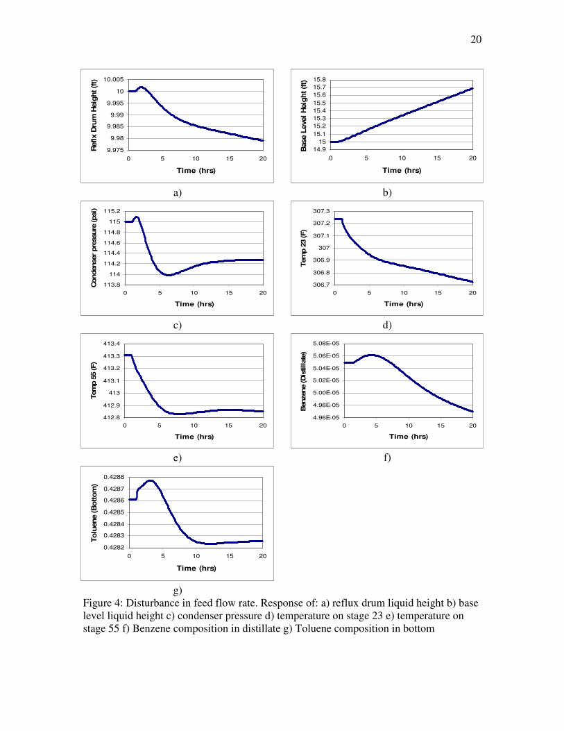
Change in feed flow rate

Figure 4 shows the response of several variables in the column in response to

disturbance in the feed flow rate without the control structures being implemented.

20

9.975

9.98

9.985

9.99

9.995

10

10.005

0 5 10 15 20

Time (hrs)

Reflx D

rum

Heig

ht (ft)

a)

14.9

15

15.1

15.2

15.3

15.4

15.5

15.6

15.7

15.8

0 5 10 15 20

Time (hrs)

Base L

evel H

eig

ht (ft)

b)

113.8

114

114.2

114.4

114.6

114.8

115

115.2

0 5 10 15 20

Time (hrs)

Condenser

pre

ssure

(psi)

c)

306.7

306.8

306.9

307

307.1

307.2

307.3

0 5 10 15 20

Time (hrs)Tem

p 2

3 (F)

d)

412.8

412.9

413

413.1

413.2

413.3

413.4

0 5 10 15 20

Time (hrs)

Tem

p 5

5 (F)

e)

4.96E-05

4.98E-05

5.00E-05

5.02E-05

5.04E-05

5.06E-05

5.08E-05

0 5 10 15 20

Time (hrs)

Benzene (D

istillate

)

f)

0.4282

0.4283

0.4284

0.4285

0.4286

0.4287

0.4288

0 5 10 15 20

Time (hrs)

Tolu

ene (B

ottom

)

g)

Figure 4: Disturbance in feed flow rate. Response of: a) reflux drum liquid height b) base

level liquid height c) condenser pressure d) temperature on stage 23 e) temperature on

stage 55 f) Benzene composition in distillate g) Toluene composition in bottom

21

Figure 4 shows that a disturbance in the feed flow rate leads to the process moving away

from its steady state, and some variables moving towards a new steady state. The base

level liquid keeps increasing until it starts flooding, at which point, the model loses its

validity.

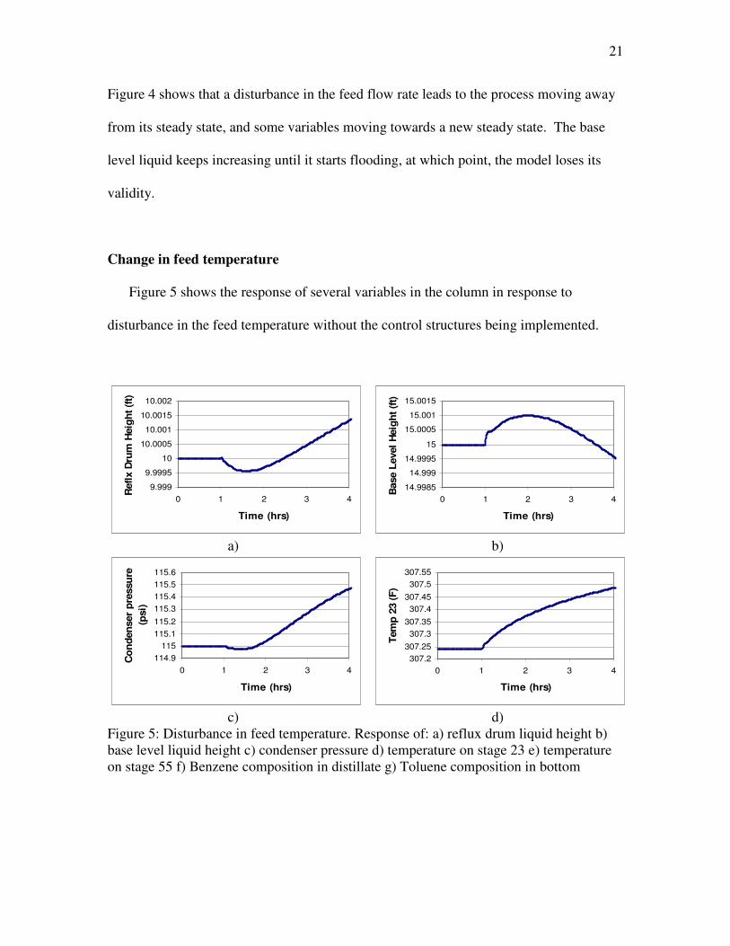
Change in feed temperature


disturbance in the feed temperature without the control structures being implemented.

9.999

9.9995

10

10.0005

10.001

10.0015

10.002

0 1 2 3 4

Time (hrs)

Refl

x D

rum

Heig

ht

(ft)

a)

14.9985

14.999

14.9995

15

15.0005

15.001

15.0015

0 1 2 3 4

Time (hrs)

Base L

evel

Heig

ht

(ft)

b)

114.9

115

115.1

115.2

115.3

115.4

115.5

115.6

0 1 2 3 4

Time (hrs)

Co

nd

en

ser

pre

ssu

re

(psi)

c)

307.2

307.25

307.3

307.35

307.4

307.45

307.5

307.55

0 1 2 3 4

Time (hrs)

Tem

p 2

3 (

F)

d)

Figure 5: Disturbance in feed temperature. Response of: a) reflux drum liquid height b)

base level liquid height c) condenser pressure d) temperature on stage 23 e) temperature

on stage 55 f) Benzene composition in distillate g) Toluene composition in bottom

22

413.25

413.3

413.35

413.4

413.45

413.5

413.55

413.6

413.65

0 1 2 3 4

Time (hrs)

Tem

p 5

5 (

F)

e)

4.99E-05

5.00E-05

5.01E-05

5.02E-05

5.03E-05

5.04E-05

5.05E-05

5.06E-05

0 1 2 3 4

Time (hrs)

Ben

zen

e (

Dii

sti

llate

)

f)

0.42856

0.42857

0.42858

0.42859

0.4286

0.42861

0.42862

0.42863

0 1 2 3 4

Time (hrs)

To

luen

e (

Bo

tto

m)

g)

Figure 5: Continued

Disturbance in the feed temperature also demonstrates that the system moves away from

steady state. The simulation results ended a little after 4 hours, this was because the

simulator had convergence problems after the disturbance was charged at the 1 hour

mark. But the results presented are just used to illustrate that the system moves away

from steady state after feed temperature disturbance.

Change in feed composition


disturbance in the feed benzene composition without the control structures being

implemented.

23

9.7

9.75

9.8

9.85

9.9

9.95

10

10.05

0 2 4 6 8 10

Time (hrs)

Refl

x D

rum

Heig

ht

(ft)

a)

14.9

15

15.1

15.2

15.3

15.4

15.5

15.6

0 2 4 6 8 10

Time (hrs)

Base L

evel

Heig

ht

(ft)

b)

108

109

110

111

112

113

114

115

116

0 2 4 6 8 10

Time (hrs)

Co

nd

en

ser

pre

ssu

re

(psi)

c)

306.2

306.4

306.6

306.8

307

307.2

307.4

0 2 4 6 8 10

Time (hrs)T

em

p 2

3 (

F)

d)

411.8

412

412.2

412.4

412.6

412.8

413

413.2

413.4

0 2 4 6 8 10

Time (hrs)

Tem

p 5

5 (

F)

e)

4.60E-05

4.70E-05

4.80E-05

4.90E-05

5.00E-05

5.10E-05

0 2 4 6 8 10

Time (hrs)

Ben

zen

e (

Dis

till

ate

)

f)

0.426

0.4265

0.427

0.4275

0.428

0.4285

0.429

0.4295

0.43

0 2 4 6 8 10

Time (hrs)

To

luen

e (

Bo

tto

m)

h)

Figure 6: Disturbance in feed benzene composition. Response of: a) reflux drum liquid

height b) base level liquid height c) condenser pressure d) temperature on stage 23 e)

temperature on stage 55 f) Benzene composition in distillate g) Toluene (bottom)

24

Figure 6 also indicates that the system deviates from its steady state after a disturbance in

the feed benzene composition.

Discussion

From the simulation results, we observe that these three types of disturbances cause

the process to deviate from its steady state values and it takes several hours before it

reaches its new steady state. This further emphasizes that a control system is necessary to

return the process to steady state within a considerable amount of time.

25

CHAPTER III

CONTROL OF A REACTIVE DISTILLATION COLUMN

Overview

Distillation is probably the most studied unit operation in terms of control. Control of

distillation columns refers to the ability of keeping certain variables at or near their

setpoints whenever there is a disturbance or set point change in the plant. Many papers

and books have been devoted to the investigation and exploration of different aspects of

distillation column control over the last half century34

. Usually, the control of reactive

distillation columns presents several difficulties due to the existence of multiple steady

states35

. Output multiplicities have direct implications for the operability and

controllability of the reactive distillation14

. Minor perturbation in feed conditions or

disturbances may produce a transition to a less favorable steady state. Sneesby et al.15

investigated different strategies to control the transition from an undesirable steady state

to a desirable one in a MTBE reactive distillation column. Sneesby et al.16

published

recommendations for the control of an ETBE reactive distillation column.

Barlett 36

studied, via dynamic simulation, different control strategies for a MTBE

reactive distillation column, and highlighted possible limitations of traditional feedback

control. A hybrid feedforward-feedback controller using molar feed ratio control was

proposed. However, the author suggested that advanced control strategy (predictive

control) would have its benefits.

Gruner et al37

described a nonlinear control scheme for continuous reactive distillation.

They designed a robust observer based on temperature measurements that was

26

incorporated into a nonlinear state feedback control scheme. Jimenez and Costa-Lopez38

analyzed the simulation, modeling, and control of a butyl acetate reactive distillation. The

authors described the process as an equilibrium stage model. They presented an efficient

decentralized control scheme with PID controllers.

Al-Arfaj and Luyben39, 40, 41, 42

conducted extensive case studies for different reactive

systems. First they investigated the control of an ideal two-product reactive distillation

column41

. The process was a two-feed 30-tray reactive distillation column. Four

components constituted the chemical system. A single reversible reaction occurred inside

the column involving two reactants and two products. The authors employed dynamic

equilibrium model to investigate six control alternative structures. In subsequent

publication40

, the authors investigated the control of a methyl acetate reactive distillation

column.

Balasubramhanya and Doyle III43

considered the production of ethyl acetate via batch

reactive distillation. They proposed a nonlinear control algorithm based on a reduced

nonlinear model, which captured the essential dynamic of the process.

The control of batch or semi-batch reactive distillation has been studied in a number of

communications. 44, 45, 46, 47, 48, 49

Sorensen et al. 50, 51

extensively studied the optimal

control of batch reactive distillation.

The procedure for determining which process variables should be controlled by

manipulating certain values is called is control strategy design52

. Dynamic simulations

can be used to provide a picture of how the plant will behave when there is a set point

change and disturbances. Controller system design can be broken into following steps:

• Formulate control objective

27

• Identify controlled and manipulated variables

• Choose a control strategy and structure

• Specify controller settings.

The control objective can generally be formulated based on safety concerns,

environmental regulations, and economic objectives. In this particular work it is mainly

driven by environmental regulations and economic considerations. The first step involved

in designing a control strategy for a distillation column is choosing the controlled and

manipulated variables. The variables are then paired based on their level of interaction

between the variables; this is achieved by performing relative gain array analysis. PI

controllers are then tuned to be implemented in the control structure. The settings of the

controllers are obtained using IMC tuning rules, the closed loop structure is tested to

investigate the control performance and identify if further tuning would be required. The

controllers are tuned until a satisfactory control performance is observed.

Choosing controlled and manipulated variables

Choosing a set of controlled and manipulated variables is the first step taken for

developing a plant wide control structure for a process. To do this, the degree of freedom

of the process must first be determined; this is the number of variables that can be

controlled. Knowing the degree of freedom of a process is useful so that you do not try to

over or under control the process.

The mathematical approach to finding the degree of freedom is to subtract the number of

independent equations from the total number of variables. An easier approach is to

simply add the total number of rationally placed control valves.

28

For instance, in a simple distillation column with a single feed, distillate and bottom

products, we have 5 control valves, one for each of the following streams: distillate,

bottom, reflux, condensing and heating medium. So this column would have 5 degrees of

freedom.

Inventories on any process must be controlled23

, these include liquid levels and

column pressure. For the case of the simple distillation column, the liquid level in both

the reflux drum and base of the column and the column of the pressure must be

controlled. Subtracting these three variables that must be controlled from 5, leaves us

with two degrees of freedom. Therefore, we are left with 2 additional variables that can

be controlled in this simple distillation case.

The remaining two variables chosen to be controlled depend on the specifications of

the process and the control resources provided for the process. Some common situations

include: controlling composition of the light-key impurity in the bottoms and the

composition of the heavy-key impurity in the distillate or controlling a temperature in the

rectifying section of the column and a temperature in the stripping section of the column.

Once all controlled variables are determined, we still have the problem of deciding what

manipulated variable to use to control what controlled variable. This “pairing” problem is

solved by performing a relative gain array (RGA) analysis which would be discussed

later.

Open loop step test

Once the controlled variables and manipulated variables are chosen, open loop tests

are performed on the column. Open loop tests are simulation runs on the dynamic column

29

carried out without any controllers in place. It can be called the natural response of the

column to changes in the manipulated variables. The responses of the controlled variables

to changes in the manipulated variables are recorded. This information is used to

determine the range in which the linear fit is appropriate and it is also used to provide the

relationship between the input and output through transfer functions.

Linearity of the model

In order to determine the transfer function relationships between input and output,

step changes in the input/manipulated variables in both directions and of different

magnitudes are simulated and the response of the output variables are used to determine

the range in which changes in the manipulated variables can be fit by linear relationships.

For instance, for similar changes in the manipulated variable in opposite directions,

should produce responses that are approximately mirror images of each other.

In this case fitting a linear transfer function would be appropriate. However if the two

responses are completely different in nature from each other then this is not a good

assumption. For large changes in the manipulated variables such a case can often be

observed. Another way to judge this could be to determine if the superposition principle

holds in the response of the controlled variables. For example for a step change of

magnitude 4, the response has to be the same as that of the addition of the two different

responses with change of magnitude 1 and change of magnitude 3 of the manipulated

variable for a linear model. Also, if a step change of magnitude 2 produces a response of

magnitude 2, a step change of twice the initial magnitude (i.e. magnitude of 4) should

30

produce a response of twice the initial response and so on. This step identifies the range

in which fitting the transfer functions will be valid.

Transfer function

The transfer function is an expression which dynamically relates the input and the

output in a process model. Y(s) = G(s) U(s) where Y is the output, U is the input and G is

the transfer function relating them. So if a transfer function is known between one input

and one output, the change in the output can be computed for a change in the input. One

important property of the transfer function is that one can calculate the steady-state

change in output given a change in input by directly setting s = 0 in G(s). Another

important property of transfer functions is that they can be added. A single process output

variable can be influenced by more than one input variable. The total output change is

calculated by summing up the changes of the output if only one of the inputs were

changed at a time.

∑=j

jiji sUsGsY )()()(

Where, )(sYi is the thi controlled variable, )(sU j is the thj manipulated variable and ijG

is the transfer function between the thi controlled variable and the thj manipulated

variable.

31

Relative Gain Array (RGA) analysis

Relative gain array was introduced by Bristol53

. Bristol developed a systematic

approach for the analysis of multivariable process control problems. The approach is

convenient because it requires only the process gain matrix K and provides two important

pieces of information54

:

1. A measure of process interactions.

2. A selection criteria for the most effective pairing of controlled and manipulated

variables.

Consider a process multivariable process with n manipulated variables and n

controlled variables. The relative gain between a controlled variable y and a manipulated

variable u is defined as the dimensionless ratio of two gains, the open-loop gain and the

closed loop gain:

( )( ) )(

)(

loopclosedgain

loopopengain

uy

uy

yji

uji

ij−

−=

∂∂

∂∂=λ

From the equation above, the numerator is a partial derivative with all the manipulated

variables held constant except ju . This is the open-loop gain ( ijK ) between iy and ju .

Similarly the denominator is evaluated with all of the control variables held constant

except iy . This is the closed-loop gain that indicates the effect of ju on iy when all other

variables are held constant.

32

The relative gain is then arranged in a relative gain array (RGA) as shown below:

4321 uuuu

=Λ

nnn

n

n

y

y

y

121

22221

11211

3

2

1

...

............

...

...

...

λλλ

λλλ

λλλ

There are fives ranges of value which an element in the RGA can have:

1. 1=ijλ . In this situation the closed-loop and open-loop gains between iy and ju

are identical. This is an ideal situation; it follows that iy and ju should be paired.

2. 0=ijλ . This indicates that the open-loop gain iy and ju is zero, therefore ju

has no effect on iy and they need not be paired.

3. 10 << ijλ . The closed-loop gain is larger than the open-loop gain. Within this

range, the interaction between the two loops is greatest when 5.0=ijλ .

4. 1>ijλ . In this situation, closing the loop reduces the gain between iy and ju .

Thus, the control loops interact. As ijλ increases, the degree of interaction

increases. When ijλ is very large, it is impossible to control multiple outputs

independently.

5. 0<ijλ . When ijλ is negative, the open-loop and closed-loop gains between iy

and ju have opposite signs. It follows that iy and ju should not be paired

because the control loops interact be trying to “fight each other” 55, 56

and the

closed-loop system may become unstable.

33

The overall recommendation from RGA analysis is to pair the controlled and

manipulated variables so that corresponding relative gains are positive and as close to one

as possible.

Tuning of controllers

After the transfer functions are derived and optimal pairing between the controlled

variable and manipulated variable are found, the controller can be tuned. First we choose

the type of controller, either P, PI or PID controller. Then the setting of the controllers is

tuned to get good control performance. PI and PID controller settings can be determined

by a number of alternative techniques. The Internal Model Control (IMC) 57

method is

one of the most commonly used methods in practice. Other methods of designing

controllers are using the Direct Synthesis (DS) 58

method, On-line tuning and other tuning

relations based on Integral Error Criteria, i.e. IAE (Integral Absolute Error), ISE (Integral

squared error) or ITAE(Integral time-weighted absolute-error) 59

.

When the controller has been tuned, it is then implemented and the control

performance is investigated.

34

CHAPTER IV

CONTROLLER DESIGN

Manipulated and controlled variables

In this process, we have six degrees of freedom: bottom flow rate, distillate flow rate,

vent flow rate, condenser duty, reboiler duty and reflux flow rate. We have the choice of

manipulating these six variables to control six other variables, we use the conventional

5X5 control structure23

, leaving one manipulated variable free. In our case, it is possible

to have two 5X5 control structures (CS1 and CS2), where the manipulated variable which

was not used in CS1 is used to substitute one of the manipulated variable initially used,

this creates the second control structure, CS2.

The manipulated variables for both control structures are given below:

For CS1,

• Bottom flow rate, distillate flow rate, vent flow rate, reboiler duty and condenser

duty.

For CS2,

• Bottom flow rate, distillate flow rate, vent flow rate, reboiler duty and reflux flow

rate.

The controlled variables chosen are the same for both control structures. The liquid levels

in both the reflux drum and base level are chosen to be controlled; the other three

variables are the pressure in the column, temperature in the stripping section and

temperature in the rectifying section.

35

Since there are 70 stages in the column, we have to decide the two stages to place the

two temperature controllers. The first stage chosen for temperature control is a stage

below the reactive zone (stage 23) and the second stage to be controlled is a stage a

quarter way up the column from the reboiler (stage 55).

Since we have chosen five manipulated variables and five controlled variables for both

control structures, RGA analysis is then used to determine which manipulated variable

would be used to control a chosen controlled variable.

Linearity of the model

In order to design the controller the transfer function fit should be done in a region

where linear relationship holds between the manipulated and controlled variables. As

discussed earlier, this means that the two responses obtained for the same controlled

variable for a given change in the manipulated variable in opposite direction should be

approximately mirror image of one another. The figures below show that the model

exhibits close to linear behavior since mirror images are derived for equal changes in

positive and negative directions. Two cases are presented by the figures below: The effect

of changing the bottom flow rate by %2.0± and the effect of changing the reboiler duty

by %05.0± . Figures 7 and 8 show the response to changes in bottom flow rate and

reboiler duty respectively.

36

14.75

14.8

14.85

14.9

14.95

15

15.05

15.1

15.15

15.2

15.25

0 1 2 3 4 5 6 7 8 9 10

Time (Hrs)

Base L

evel H

eig

ht

(ft)

+0.2% -0.2%

Figure 7: Response of base level height to changes in bottom flow rate

307

307.05

307.1

307.15

307.2

307.25

307.3

307.35

307.4

307.45

0 2 4 6 8 10

Time (Hrs)

Te

mp

23

(F

)

+0.05% -0.05%

Figure 8: Response of temperature on stage 23 to changes in reboiler duty

The responses of other controlled variable to changes in the manipulated variables

give similar results, showing the linearity of the model.

37

Transfer functions

We also perform open loop tests to obtain transfer functions between manipulated

variables and controlled variables. A transfer function is an expression which

dynamically relates the input and the output of a process model. Y(s) = G(s) U(s) where

Y is the output, U is the input and G is the transfer function relating them. Accordingly if

a transfer function is known between one input and output, the change in the output can

be computed for a change in the input. In this particular study there are five input

variables which are the manipulated variables and five output variables which are the

controlled variables. As a result of this a 5 X 5 control structure there will have 25

transfer functions since each combination of input-output variables results in one transfer

function. From our simulations, we obtained responses to step changes in the manipulated

variables and from the figures we obtained the transfer functions.

Figure 9 shows the response of the five controlled variables to change in bottom flow

rate.

9.9997

9.99975

9.9998

9.99985

9.9999

9.99995

10

10.00005

0 5 10 15 20

Time (Hrs)

Reflux D

rum

Heig

ht (f

t)

a)

14.5

14.55

14.6

14.65

14.7

14.75

14.8

14.85

14.9

14.95

15

15.05

0 5 10 15 20

Time (Hrs)

Base L

evel H

eig

ht (f

t)

b)

Figure 9: Change in bottom flow rate. Open loop response of: a) reflux drum liquid


temperature on stage 55

38

114.965

114.97

114.975

114.98

114.985

114.99

114.995

115

115.005

0 5 10 15 20

Time (Hrs)

Condenser Pre

ssure

(Psi)

c)

307.226

307.228

307.23

307.232

307.234

307.236

307.238

307.24

307.242

0 5 10 15 20

Time (Hrs)

Tem

p 2

3 (F)

d)

413.288

413.29

413.292

413.294

413.296

413.298

413.3

413.302

413.304

413.306

0 5 10 15 20

Time (Hrs)

Tem

p 5

5 (F)

e)

Figure 9: Continued

Figure 9 shows the transfer function profile for the five measured variables to changes in

the bottom flow rate. From the figure above, we can see that a change in the bottom flow

rate has an effect on each controlled variable. But each response varies in regards to the

extent on which it is affected by the bottom flow rate. The reflux drum and base level

liquid height respond as an integrating process, i.e. the process increases with time an

does not reach a steady state. If allowed to continue over a long period of time, the two

liquid drums will start drying up. The condenser pressure, temperature on stage 23 and 55

has a first-order process response. As it can be seen in the figure 9, the three latter

variables reach a new steady state. Also we see that there are variables not really affected

by the bottom flow rate change compared to other variables. The base level liquid height

39

change is much more than the change in the reflux drum’s liquid height. Also the

pressure and temperature do not change much in magnitude.

Figure 10 shows the response of five controlled variables to a change in distillate flow

rate.

9.88

9.9

9.92

9.94

9.96

9.98

10

10.02

0 5 10 15 20

Time (Hrs)

Reflux D

rum

Heig

ht (ft)

a)

14.9999

15

15.0001

15.0002

15.0003

15.0004

15.0005

15.0006

15.0007

0 5 10 15 20

Time (Hrs)

Base L

evel H

eig

ht (f

t)

b)

114.965

114.97

114.975

114.98

114.985

114.99

114.995

115

115.005

0 5 10 15 20

Time (Hrs)

Condenser Pre

ssure

(Psi)

c)

307.2386

307.2388

307.239

307.2392

307.2394

307.2396

307.2398

307.24

307.2402

307.2404

307.2406

0 5 10 15 20

Time (Hrs)

Tem

p 2

3 (F)

d)

Figure 10: Change in distillate flow rate. Open loop response of: a) reflux drum liquid



40

413.302

413.3025

413.303

413.3035

413.304

413.3045

0 5 10 15 20

Time (Hrs)

Tem

p 5

5 (F)

e)

Figure 10: Continued

The distillate flow rate change also gives an integrating process response for both reflux

drum and base level liquid height. An increase in the distillate flow rate causes the reflux

drum liquid level to reduce, if the process is let to run for a long period of time, the reflux

drum would dry up while the base (reboiler) drum would flood. The other three variables

respond with a first-order process. Changes in the pressure, temperature and base level

liquid height are negligible compare to the change in the reflux drum liquid height. Some

of the changes are so small that the profile appears as steps, these steps are numerical

problems and not physical. We can infer that the distillate flow rate would be used to

control the reflux drum liquid height, but we leave assumptions for analysis that would

actually give optimal pairing of the variables in the process. This would be achieved by

RGA analysis.

Figure 11 shows the response of five controlled variables to change in vent flow rate.

41

9.992

9.993

9.994

9.995

9.996

9.997

9.998

9.999

10

10.001

0 5 10 15 20

Time (Hrs)

Reflux D

rum

Heig

ht (f

t)

a)

14.999

15

15.001

15.002

15.003

15.004

15.005

15.006

15.007

15.008

15.009

0 5 10 15 20

Time (Hrs)

Base L

evel H

eig

ht (f

t)

b)

114.55

114.6

114.65

114.7

114.75

114.8

114.85

114.9

114.95

115

115.05

0 5 10 15 20

Time (Hrs)

Condenser Pre

ssure

(Psi)

c)

307.215

307.22

307.225

307.23

307.235

307.24

307.245

0 5 10 15 20

Time (Hrs)

Tem

p 2

3 (F)

d)

413.275

413.28

413.285

413.29

413.295

413.3

413.305

413.31

0 5 10 15 20

Time (Hrs)

Tem

p 5

5 (F)

e)

Figure 11: Change in vent flow rate. Open loop response of: a) reflux drum liquid height

b) base level liquid height c) condenser pressure d) temperature on stage 23 e)


We would expect a change in the vent flow rate to have a visible effect on the pressure of

the column, since it means either reducing or increasing the amount of vapor in the

column. Figure 11 shows that increasing the vent flow rate, letting more vapor out of the

42

system, would reduce the condenser pressure. This reduction in pressure is so far the

largest out of the three manipulated variables noticed, and has the fastest response. The

temperatures on both stages studied are reduced but not profoundly, and the two liquid

levels show an integrating process response.

Figure 12 shows the response of the five controlled variables to a change in the

reboiler duty.

9.999

9.9995

10

10.0005

10.001

10.0015

10.002

10.0025

10.003

10.0035

10.004

10.0045

0 5 10 15 20

Time (Hrs)

Reflux D

rum

Heig

ht (f

t)

a)

14.993

14.994

14.995

14.996

14.997

14.998

14.999

15

15.001

0 5 10 15 20

Time (Hrs)

Base L

evel H

eig

ht (f

t)

b)

114.9

115

115.1

115.2

115.3

115.4

115.5

0 5 10 15 20

Time (Hrs)

Condenser Pre

ssure

(Psi)

c)

307.2

307.25

307.3

307.35

307.4

307.45

307.5

0 5 10 15 20

Time (Hrs)

Tem

p 2

3 (F)

d)

Figure 12: Change in reboiler duty. Open loop response of: a) reflux drum liquid height



43

413.25

413.3

413.35

413.4

413.45

413.5

413.55

0 5 10 15 20

Time (Hrs)

Tem

p 5

5 (F)

e)


An increase in the reboiler duty in the column, increases the temperature in the column,

produces more vapor, and hence increases the column pressure. It boils more liquid in the

base level drum, so the liquid height reduces and if let to continue for a long period of

time, dries up. These are behaviors that are expected, but there are some aspects of the

column we can not explicitly state without performing the simulation and observing hoe

they respond, but from figure 12, we see that the liquid height in the reflux drum

increases as the reboiler duty increases.

Figure 13 shows the response of the five controlled variables to a change in the

condenser duty.

44

9.95

9.955

9.96

9.965

9.97

9.975

9.98

9.985

9.99

9.995

10

10.005

0 5 10 15 20

Time (Hrs)

Reflux D

rum

Heig

ht (f

t)

a)

14.99

15

15.01

15.02

15.03

15.04

15.05

15.06

15.07

0 5 10 15 20

Time (Hrs)

Base L

evel H

eig

ht (f

t)

b)

110

110.5

111

111.5

112

112.5

113

113.5

114

114.5

115

115.5

0 5 10 15 20

Time (Hrs)

Condenser Pre

ssure

(Psi)

c)

306.4

306.5

306.6

306.7

306.8

306.9

307

307.1

307.2

307.3

0 5 10 15 20

Time (Hrs)

Tem

p 2

3 (F)

d)

412.3

412.4

412.5

412.6

412.7

412.8

412.9

413

413.1

413.2

413.3

413.4

0 5 10 15 20

Time (Hrs)

Tem

p 5

5 (F)

e)

Figure 13: Change in condenser duty. Open loop response of: a) reflux drum liquid height



Increasing the condenser duty, reduces the temperature in the column, also condenses

more vapor, therefore reducing the vapor in the column, hence reducing the pressure. It

has an integrating-process response on both liquid levels in the column. Changes in the

45

condenser duty and reboiler duty show that these manipulated variables have more of an

effect on the temperature on both stages than the first three manipulated variables studied.

Figure 14 below shows the response of the five controlled variables to a change in the

reflux flow rate.

9.996

9.9965

9.997

9.9975

9.998

9.9985

9.999

9.9995

10

10.0005

0 5 10 15 20

Time (Hrs)

Reflux D

rum

Heig

ht (f

t)

a)

14.999

15

15.001

15.002

15.003

15.004

15.005

15.006

15.007

15.008

0 5 10 15 20

Time (Hrs)

Base L

evel H

eig

ht (f

t)

b)

114.98

115

115.02

115.04

115.06

115.08

115.1

115.12

0 5 10 15 20

Time (Hrs)

Condenser Pre

ssure

(Psi)

c)

307.205

307.21

307.215

307.22

307.225

307.23

307.235

307.24

307.245

0 5 10 15 20

Time (Hrs)

Tem

p 2

3 (F)

d)

Figure 14: Change in reflux flow rate. Open loop response of: a) reflux drum liquid



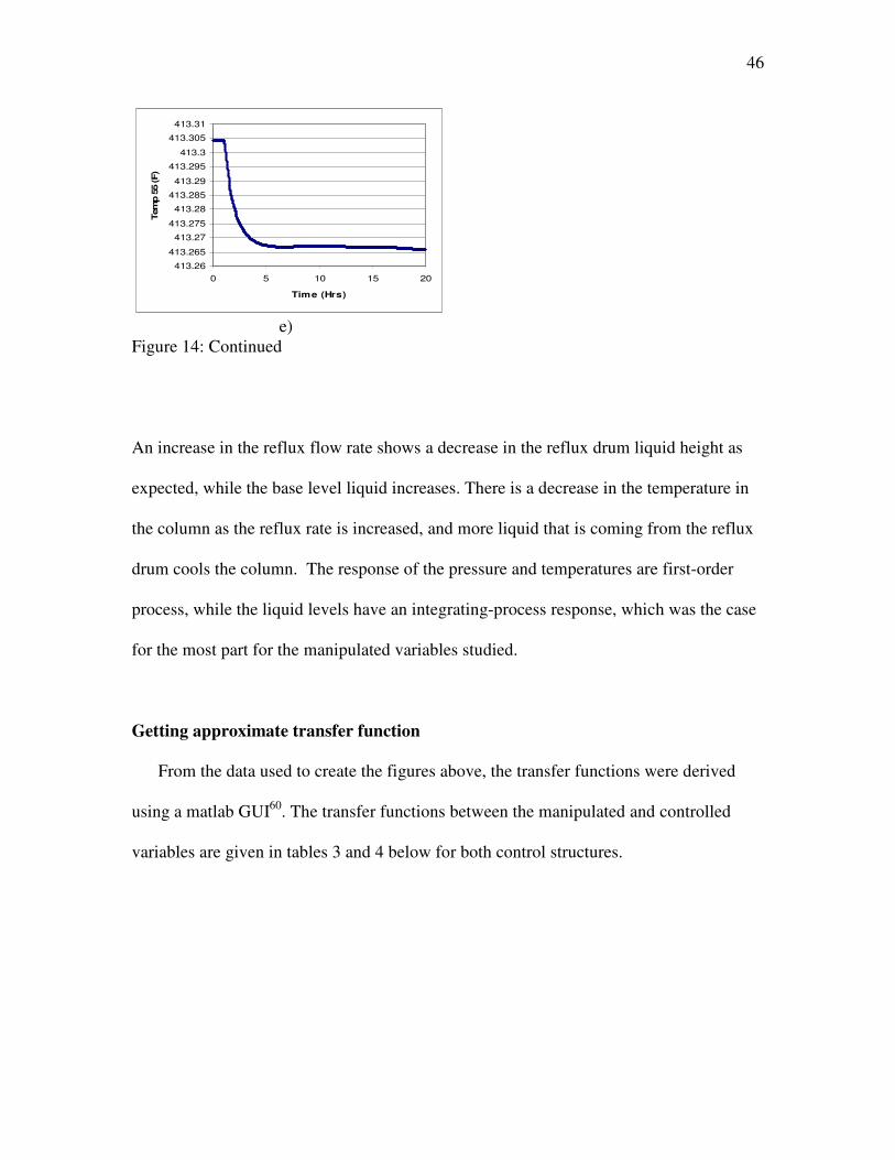
46

413.26

413.265

413.27

413.275

413.28

413.285

413.29

413.295

413.3

413.305

413.31

0 5 10 15 20

Time (Hrs)

Tem

p 5

5 (F)

e)


An increase in the reflux flow rate shows a decrease in the reflux drum liquid height as

expected, while the base level liquid increases. There is a decrease in the temperature in

the column as the reflux rate is increased, and more liquid that is coming from the reflux

drum cools the column. The response of the pressure and temperatures are first-order

process, while the liquid levels have an integrating-process response, which was the case

for the most part for the manipulated variables studied.

Getting approximate transfer function

From the data used to create the figures above, the transfer functions were derived

using a matlab GUI60

. The transfer functions between the manipulated and controlled

variables are given in tables 3 and 4 below for both control structures.

47

Table 3: Transfer functions for control structure 1.

Reflux Drum Height (ft) Base Level Height

(ft)

Condenser

Pressure (psi)

Temp 23 (F) Temp 55 (F)

Bottom

Flow Rate 1189.8

)1232.1(1068.8 554.07

+

+−×− −−

s

ess

s

51053.8 −×−

1437.2

1004.1 07.14

+

×− −−

s

es

1561.2

1045.4 5

+

×− −

s 1622.2

109.4 5

+

×− −

s Distillate

Flow Rate s

5102.4 −×−

s

es183.071078.2 −−×

15843.0

1057.2 4

+

×− −

s s

es116.061027.2 −−×−

1654.2

1058.1 565.05

+

×− −−

s

es

Vent Flow

Rate s

41001.1 −×−

s

es184.041013.1 −−×

1582.0

1005.1 1

+

×− −

s 1205.6

1072.5 245.03

+

×− −−

s

es

1798.2

1043.6 56.03

+

×− −−

s

es

Reboiler

Duty 1249.8

)1249.1(1059.1 49.07

+

+−× −−

s

ess

s

es978.081041.1 −−×−

1445.2

1088.1 07.15

+

× −−

s

es

1646.2

1011.8 6

+

× −

s 1646.2

1092.8 6

+

× −

s Condenser

Duty 1463.8

1062.3 7

+

×− −

s s

es325.08108.2 −−×

1925.1

1064.3 5

+

×− −

s 1505.3

1099.5 56.06

+

×− −−

s

es

1907.2

1052.7 545.06

+

×− −−

s

es

48

Table 4: Transfer functions for control structure 2.

Reflux Drum Height (ft) Base Level Height

(ft)

Condenser

Pressure (psi)

Temp 23 (F) Temp 55 (F)

Bottom

Flow

Rate 1189.8

)1232.1(1068.8 554.07

+

+−×− −−

s

ess

s

51053.8 −×−

1437.2

1004.1 07.14

+

×− −−

s

es

1561.2

1045.4 5

+

×− −

s 1622.2

109.4 5

+

×− −

s

Distillate

Flow

Rate s

5102.4 −×−

s

es183.071078.2 −−×

15843.0

1057.2 4

+

×− −

s s

es116.061027.2 −−×−

1654.2

1058.1 565.05

+

×− −−

s

es

Vent

Flow

Rate s

41001.1 −×−

s

es184.041013.1 −−×

1582.0

1005.1 1

+

×− −

s 1205.6

1072.5 245.03

+

×− −−

s

es

1798.2

1043.6 56.03

+

×− −−

s

es

Reboiler

Duty 1249.8

)1249.1(1059.1 49.07

+

+−× −−

s

ess

s

es978.081041.1 −−×−

1445.2

1088.1 07.15

+

× −−

s

es

1646.2

1011.8 6

+

× −

s 1646.2

1092.8 6

+

× −

s Reflux

Flow

Rate s

61034.5 −×−

s

51017.1 −×

19306.0

1012.3 158.03

+

× −−

s

es

1755.1

1025.8 4

+

×− −

s 19472.0

1004.1 3

+

×− −

s

49

Relative Gain Array (RGA) analysis

Given the gain of each manipulated variable (input) with corresponding controlled

variable (output), we can compute the relative gain array. We place the gain for both

control structures in a 5X5 matrix. Since the reactive distillation column is integrating,

steady-state gains are not defined for the reflux drum liquid level or for the reboiler

liquid volume. However, some information regarding these variables is required for

computing the RGA. The approach initially developed by Woolverton61

and further

described by McAvoy55

is employed. For variables that exhibit integrating responses, the

RGA is calculated based on the derivatives of the variables with respect to time. The

gain matrix for both structure are given in the tables 5 and 6:

Table 5: Gain matrix: control structure 1

Reflux Drum Base Level Condenser

Pressure

Temp 23 Temp 55

Bottom -8.67937E-07 -0.001621578 -0.00010501 -4.54E-05 -4.96E-05

Distillate -0.000806092 5.08228E-06 -0.000259113 -1.42E-05 -1.58E-05

Vent -0.001892057 0.00209201 -0.105975164 -0.005724 -0.006498

Reboiler 1.58697E-07 -2.52936E-07 1.90273E-05 8.18E-06 9E-06

Condenser -3.61953E-07 5.21349E-07 -3.69595E-05 -6.08E-06 -7.6E-06

Table 6: Gain matrix: control structure 2

Reflux Drum

Level

Base Level Condenser

Pressure

Temp 23 Temp 55

Bottom -8.67937E-07 -0.001621578 -0.00010501 -4.54E-05 -4.96E-05

Distillate -0.000806092 5.08228E-06 -0.000259113 -1.42E-05 -1.58E-05

Vent -0.001892057 0.00209201 -0.105975164 -0.005724 -0.006498

Reboiler 1.58697E-07 -2.52936E-07 1.90273E-05 8.18E-06 9E-06

Reflux -9.86584E-05 0.000209569 0.00311582 -0.000906 -0.001064

Performing Relative Gain Array analysis on the gain matrix above, the pairing of

variables can be achieved. The relative gain arrays for both control structures are given

50

in tables 7 and 8 for CS1 and CS2 respectively, with the recommended pairings in bold.

Tables 9 and 10 shows each controlled variable paired with its respective manipulated

variable, for both CS1 and CS2 respectively.

Table 7: Relative Gain Array: control structure 1

Reflux

Drum

Base Level Condenser

Pressure

Temp 23 Temp 55

Bottom -5.3E-08 0.999108 0.00136 0.004437 -0.00491

Distillate 1.005854 -3.1E-07 -0.00637 -0.00394 0.004454

Vent -0.00597 0.000121 1.21562 1.652735 -1.8625

Reboiler -4.7E-05 0.000902 -0.11775 7.079145 -5.96225

Condenser 0.000164 -0.00013 -0.09286 -7.73238 8.825206

Table 8: Relative Gain Array: control structure 2

Reflux Drum Base Level Condenser

Pressure

Temp 23 Temp 55

Bottom 7.48379E-07 0.999937 0.000821 -0.11351 0.112751

Distillate 1.00486034 3.16E-06 -0.0046 0.045323 -0.04559

Vent -0.005225767 -0.00034 0.983576 -4.69163 4.71362

Reboiler -0.000124644 0.000971 -0.06571 18.40463 -17.3398

Reflux 0.000489323 -0.00058 0.085908 -12.6448 13.55899

Table 9: Controlled variable paired with corresponding manipulated variable for CS1

Controlled Variable Manipulated Variable

Base level height Bottom flow rate

Reflux drum level height Distillate flow rate

Condenser pressure Vent flow

Temperature (Stage 23) Reboiler duty

Temperature (Stage 55) Condenser duty

Table 10: Controlled variable paired with corresponding manipulated variable for CS2

Controlled Variable Manipulated Variable

Base level height Bottom flow rate

Reflux drum level height Distillate flow rate

Condenser pressure Vent flow

Temperature (Stage 23) Reboiler duty

Temperature (Stage 55) Reflux flow rate

51

According to Bristol’s recommendation for controller pairing, controlled variables

and manipulated variables are paired so that the corresponding relative gains are positive

and as close to one as possible. From the above table, the two control structures have

similar controller pairing except for the difference of the manipulated variables used for

controlling the temperature on stage 55. From the controller pairing and the transfer

function the controllers can now be tuned. Figure 15 shows the process flow diagram of

the two control structures.

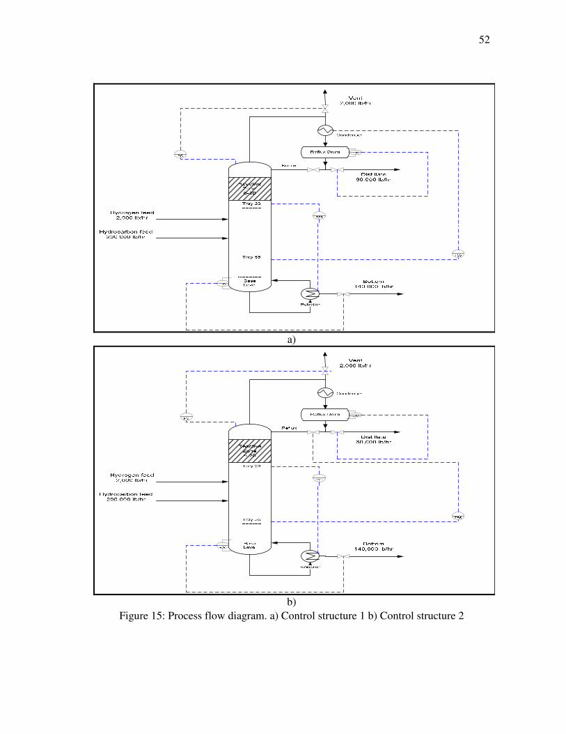
52

a)

b)

Figure 15: Process flow diagram. a) Control structure 1 b) Control structure 2

53

CHAPTER V

CONTROL STRUCTURE OF REACTIVE DISTILLATION WITH PI

CONTROLLERS

Controller tuning

Before the controllers are implemented, they have to be tuned to provide good

controller performance for the dynamic process. From the pairing recommended by the

RGA analysis, we have 5 controllers to tune and from the transfer function for paired

variables we can get an initial value of the controller parameters by using IMC tuning

method. Since the process is simulated in Aspen Dynamics, the units of the gains have

to be converted from the respective units to (%/%). The gain, time constant and time

delay are then used to calculate the controller gain and reset time. The choice of the

desired closed-loop time constant has to be taken into consideration, because it is used to

calculate the controller parameters. Choosing a small desired closed-loop time constant

will lead to a more aggressive controller that would return the process back to its steady

state within a considerably shorter amount of time than choosing a larger time constant.

Also, we do not want to choose a very small desired closed-loop time constant that will

lead to the system being oscillatory and unstable when a disturbance is charged into the

system. There are several rules of thumbs in choosing a desired closed-loop time

constant57

. Tables 11 and 12, show the parameter for each controller for both control

structure. As a rule of thumb, the desired closed loop constant should be smaller than the

open-loop time constant and greater than the delay time: θττ >> c .62

54

Table 11: Control settings for control structure 1 using IMC tuning rules

Reflux

Level

Controller

Base Level

Controller

Pressure

Controller

Stage 23

Temperature

Controller

Stage 55

Temperature

Controller

Controller

gain (%/%)

70.73

23.77 50.00 13.24 90.00

Reset time

(hr)

0.22 0.22 0.001 0.10 0.25

Table 12: Control settings for control structure 2 using IMC tuning rules

Reflux

Level

Controller

Base Level

Controller

Pressure

Controller

Stage 23

Temperature

Controller

Stage 55

Temperature

Controller

Controller

gain (%/%)

74.28 24.16 50.00 8.76 10.00

Reset time

(hr)

0.22 0.22 0.001 0.11 0.06

The control structure is implemented and the performance is investigated.

Disturbance rejection is investigated for each controller in both control structures.

Disturbances charged to the column are feed flow rate, feed temperature and feed

composition.

Control performance

Table 13: Disturbances to system

Perturbation Description

D1 Reformate feed flow rate +5%

D2 Feed Temperature +10%

D3 Feed benzene composition from 0.08 to 0.09

For the perturbations in Table 13, closed-loop responses are simulated in Aspen

Dynamics and the control performance of both structures are assessed and compared.

55

Figure 16 shows the closed loop response of both control structures to disturbance in

the feed flow rate.

9.997

9.998

9.999

10

10.001

10.002

10.003

0 5 10 15 20

Time (hrs)

Re

flu

x D

rum

He

igh

t (f

t)

CS1 CS2

a)

14.998

15

15.002

15.004

15.006

15.008

0 5 10 15 20

Time (hrs)

Ba

se

Le

ve

l H

eig

ht

(ft)

CS1 CS2

b)

114.9996

114.9998

115

115.0002

115.0004

115.0006

115.0008

0 5 10 15 20

Time (hrs)Co

nd

en

se

r P

res

su

re (

ps

i)

CS1 CS2

c)

307.16

307.18

307.2

307.22

307.24

307.26

0 5 10 15 20

Time (hrs)

Te

mp

23

(F

)

CS1 CS2

d)

413.22413.24413.26413.28413.3

413.32413.34413.36

0 5 10 15 20

Time (hrs)

Te

mp

55

(F

)

CS1 CS2

e)

Figure 16: Feed flow rate disturbance (D1). Closed loop response to a) reflux drum liquid



56

Figure 17 below shows the closed loop response of both control structures to

disturbances in feed temperature.

9.985

9.99

9.995

10

10.005

10.01

10.015

0 5 10 15

Time (hrs)

Re

flu

x D

rum

He

igh

t (f

t)

CS1 CS2

a)

14.98514.99

14.99515

15.00515.01

15.01515.02

0 5 10 15

Time (hrs)

Ba

se

Le

ve

l H

eig

ht

(ft)

CS1 CS2

b)

114.994

114.996

114.998

115

115.002

115.004

0 5 10 15

Time (hrs)Co

nd

en

se

r P

res

su

re (

ps

i)

CS1 CS2

c)

307

307.2

307.4

307.6

307.8

308

308.2

0 5 10 15

Time (hrs)

Te

mp

23

(F

)

CS1 CS2

d)

412.8

413

413.2

413.4

413.6

413.8

0 5 10 15

Time (hrs)

Te

mp

55

(F

)

CS1 CS2

e)

Figure 17: Feed temperature disturbance (D2). Closed loop response to a) reflux drum

liquid height b) base level liquid height c) condenser pressure d) temperature on stage 23

e) temperature on stage 55

57

Figure 18 shows the closed loop response of both control structures to disturbances

in feed benzene composition.

9.985

9.99

9.995

10

10.005

10.01

0 10 20 30

Time (hrs)

Refl

ux D

rum

Heig

ht

(ft)

CS1 CS2

a)

14.998

15

15.002

15.004

15.006

15.008

15.01

15.012

0 10 20 30

Time (hrs)

Base L

evel H

eig

ht

(ft)

CS1 CS2

b)

114.9985

114.999114.9995

115

115.0005115.001

115.0015115.002

115.0025

0 10 20 30

Time (hrs)

Co

nd

en

ser

Pre

ssu

re (

psi)

CS1 CS2

c)

307.15

307.2

307.25

307.3

307.35

307.4

0 10 20 30

Time (hrs)

Tem

p 2

3 (

F)

CS1 CS2

d)

413

413.1

413.2

413.3

413.4

413.5

0 10 20 30

Time (hrs)

Tem

p 5

5 (

F)

CS1 CS2

e)

Figure 18: Feed benzene composition disturbance (D1). Closed loop response to a) reflux

drum liquid height b) base level liquid height c) condenser pressure d) temperature on

stage 23 e) temperature on stage 55

58

Discussion

The controller settings above give a satisfactory controller performance. From the

figures above, the controllers are returning each controlled variable back to steady state

in less than 5 hrs. Control structure 2 generally performs better than control structure 1,

it is less oscillatory and it gets back to steady state faster. Perturbation (D3) is where the

advantage of CS2 over CS1 is emphasized. It takes CS1 about 25 hours to return to

steady state after a feed composition disturbance, whereas CS2 returns the column to

steady state in approximately 3 hours.

59

CHAPTER VI

CONCLUSIONS AND RECOMMENDATIONS

Conclusions

The dynamic model of a reactive distillation column for benzene hydrogenation

was created and investigated. The column has 70 trays and is fed with a stream that

contains 12 components. Hydrogen was fed above the hydrocarbon feed stage to

hydrogenate the benzene in the process. The feed to the system comes from a reformer

and may change on a regular basis which presents a need for investigating the dynamic

behavior of the process. EPA regulations require that the benzene content in the distillate

streams leaving the column is below 1% weight concentration even under the influence

of large disturbances in the feed. Building a dynamic model started by creating a steady

state model for the process. The results from the steady state simulation were compared

with data provided from an industrial collaborator. The steady state results were then

extended to be used to create the dynamic model, which is used to design the control

structure for the process.

Open loop tests were performed on the dynamic model for different disturbances

and the need for the work was revealed as the process moves away from its steady state,

hence the need for a control system. A set of manipulated and controlled variables were

chosen and open loop simulations were carried out to determine the transfer functions

between the variables.

60

A 5x5 control structure was implemented on the process and investigated. Two

control structures were compared and analyzed. RGA analysis was performed on the

dynamic model to find optimal pairing for the control structures. Naturally, the RGA

analysis suggested pairing the condenser pressure with the vent flow rate, the base level

liquid height with the bottom flow rate and the reflux drum liquid level with the distillate

flow rate. The three pairing are in agreement with studies dedicated to distillation or

reactive distillation.24, 63

The other two variables are used to control the temperature on

two different stages (stage 23 and 55).

PI controllers were designed and tuned based upon the transfer function between the

manipulated and the controlled variable and the IMC tuning rules were used to obtain

the controller settings. The controllers provided satisfactory control performance, where

all the control variables return to steady state within 5 hours of when disturbance was

charged.

From our results, control structure 2 performed better than control structure 1. The

main advantage of CS2 over CS1 is noticed in the simulation of feed composition

disturbance rejection, where CS2 returns all variables back to steady state within 3 hrs

while it take CS1 more than 20 hrs to return the temperature variables back to steady

state. This means, it would better to control the temperature on stage 55 with the reflux

flow rate rather than the condenser duty.

There is a possibility the control performance can be further improved by

investigating feed forward and cascade control and also trying to implement model

predictive control (MPC) for the column.

61

This is one of the first works on the control of a reactive distillation for benzene

hydrogenation, in our approach we used temperature controllers as opposed to

conventional composition controllers used in simulation but hardly used in real-life

situations.

Future work

The 5x5 control of a benzene hydrogenation reactive distillation column was

investigated however supplemental research and simulations can be done to extend the

work done here. The following issues are worth of investigation:

• Choosing different sets of manipulated and controlled variables to investigate if it

gives any advantage to the existing control structure developed.

• Feed forward control studies can be implemented on the process, to investigate if it

improves the process controllability.

• Cascade control structures can also be investigated on the process.

• Also implementing model predictive control (MPC) on the column may have its

advantages, so it should be taken into consideration for investigation.

62

REFERENCES

1. Sundmacher, K.; Kienle, A. Reactive distillation: Status and future directions.

WILEY-VCH Verlag GmbH & Co. KGaA: Weinheim, 2003.

2. Agreda, V.H.; Partin, L.R.; Heise, W.H. Chem. Eng. Progr. 1990, 86, 40-46.

3. Siirola, J.J. AICHE Symp. Ser. 1995, 91, 222-233.

4. Smith, L.A. US Patent No. 4.978.807, 1990.

5. Stankiewicz, A. Chem. Eng. Progr. 2003, 42, 137-144.

6. Sundmacher, K.; Rihko, L.K.; Hoffmann, U. Chem. Eng. Comm. 1994, 127, 151-

167.

7. Taylor, R.; Krishna, R. Chemical Engineering Science. 2000, 55, 5183-5229.

8. Chakrabarty, A. M.S. Thesis, Texas A&M University, 2004.

9. Gilbert, G.R.; Hearn, D.; Putman, H.M. US Pat. 57,73,670, 1998.

10. Rock, K.; Gildert, G. H.; Meguirk T. Chem. Engng. New York., 1997, July, 78-

82.

11. Sneesby, M.G.; Tade, M.O.; Smith, T.N. J. Proc. Control. 1999, 9, 19-31.

12. Sneesby, M.G.; Tade, M.O.; Smith, T.N. In Proc. 1997 Symp. Distillation and

Absorption. 1997, 205-216.

13. Sneesby, M.G.; Tade, M.O.; Smith, T.N. Computers Chem. Eng. 1998, 22, 879-

892.

14. Sneesby, M.G.; Tade, M.O.; Datta, R.; Smith, T.N. Indust. & Eng. Chem.

Research. 1997, 36, 1870-1881.

15. Sneesby, M.G.; Tade, M.O.; Smith, T.N. Chem. Eng. Res. & Design, Trans

IchemE, Part A. 2000, 78, 283-292.

16. Tade, M.O; Tian, Y. Separation and Purification Technology. 2000, 19, 85-91.

17. Tian, Y.; Zhao, F.; Biswarno, B.H.; Tade, M.O. J. Proc. Control. 2003, 13, 57-

67.

63

18. Bock, H.; Wozny, G.; Gutsche, B. Chemical Engineering and Processing. 1997,

36, 101-109.

19. Kumar, A.; Daoutidis, P. AIChE 1999, 45, 51.

20. Vora, N.; Daoutidis, P. Ind. Eng. Chem. Res. 2001, 40, 833.

21. Lextrait, S. W. Ph.D. Dissertation, The University of Texas at Austin, 2003.

22. Al-Arfaj, M.A.; Luyben, W.L. Indust. & Eng. Chem. Research. 2000, 39, 3298-

3307.

23. Taylor, R.; Krishna, R.; Kooijman H. Chemical Engineering Progress 2003,

July, 28-39.

24. Lee, J.-H.; Dudukovic, M. P. Computers Chem Engng 1998, 23, 159-172.

25. Rouzineau, D.; Prevost, M.; Meyer, M. In EFCE Distillation & Absorption,

Working Party, Cedex, France, 2000.

26. Skogestad, S. Trans I.Chem.E 1997, 75, 539- 562.

27. Aspen Plus, Release AspenONE, Aspen Technology, Inc.: Cambridge, MA,

2004.

28. Hangos, K.M.; Cameron, I.T. Computers Chem. Engng. 2001, 25, 237-255.

29. Brenan, K. E.; Campbell, S. L.; Petzold, L. R. Numerical Solution of Initial-

Value Problems in Differential- Algebraic Equations.; SIAM: Philadelphia,

1996.

30. Moe, H. I. Ph.D. Dissertation, University of Trondheim, Norway, 1995.

31. Moe, H. I.; Hauan, S.; Lien, K. M.; Hertberg, T. Computers Chem Engng, 1995,

19, S513- S518.

32. Ponton, J.W.; Gawthrop, P.J. Computers Chem. Engng. 1991, 15, 803-808.

33. Aspen Dynamics, Release AspenONE, Aspen Technology, Inc.: Cambridge, MA,

2004.

34. Luyben, W.L. In Practical Distillation Control; Luyben, W. L., Ed.; Van

Nostrand Reinhold: New York, 1992.

64

35. Wang, S.J.; Wong, D.S.H.; Lee, E.K. Journal of Process Control. 2003, 13, 503-

515.

36. Bartlett, D.A. In FOCAPO Proceedings. 1998, July, 315-321.

37. Gruner, S.; Mohl, K.D.; Kienle, A.; Gilles, E.D.; Fernholz, G.; Friedrich, M.

Control Engineering Practice. 2003, 11, 915-925.

38. Jimenez, L.; Costa-Lopez, J. I&EC Research. 2002, 41, 6735-6744.

39. Al-Arfaj, M.A.; Luyben, W.L. I&EC Research. 2000, 39, 3298-3307.

40. Al-Arfaj, M.A.; Luyben, W.L. Chemical Engineering Science. 2002, 57, 5039-

50550.

41. Al-Arfaj, M.A.; Luyben, W.L. AIChE. 2002, 48, 905-908.

42. Al-Arfaj, M.A.; Luyben, W.L. I&EC Research. 2002, 41, 3784-3796.

43. Balasubramhanya, L.S.; Doyle III, F.J. Journal of Process Control. 2000, 10,

209-218.

44. Cervantes, A.M.; Wachter, A.; Tutuncu, R.H.; Biegler, L.T. Computers Chem.

Engng. 2000, 24, 39-51.

45. Engell, S.; Fernholz, G. Chemical Engineering and Processing. 2003, 42, 201-

210.

46. Fernholz, G.; Engell, S.; Kreul, L.U.; Gorak, A. Computers Chem. Engng. 2000,

24, 1569-1575.

47. Fernholz, G.; Wang, W.; Engell, S.; Fougner, K.; Bredehoft, J. In Proc.

International Conference on Control Applications in Kohala Coast-Island of

Hawaii. 1999, 397-402.

48. Sorensen Leversund, E.; Macchietto, S.; Stuart, G.; Skogestad, S. Computers

Chem. Engng. 1994, 18 Suppl, S391-S395.

49. Monroy-Loperena, R.; Alvarez-Ramirez, J. I&EC Research. 2000, 39, 378-386.

50. Sorensen, E.; Macchietto, S.; Stuart, G.; Skogestad, S. Computers Chem. Engng.

1996, 20, 1491-1498.

65

51. Sorensen, E.; Skogestad, S. Journal of Process Control. 1994, 4, 205-217.

52. Vogel, E. F. Plantwise In Practical Distillation Control Luyben, W. L., Ed.; Van

Nostrand Reinhold: New York, 1992.

53. Bristol, E. H. IEEE Transactions on Automatic Control 1966, 11, 133-134.

54. Seborg, D.E.; Edgar, T.F.; Mellichamp, D.A. Process Dynamics and Control, 2d

ed., John Wiley & Sons, Inc.: Hoboken, NJ, 2004.

55. McAvoy, T.J. Interaction Analysis Principles and Applications. Instrument

Society of America: Research Triangle Park, NC, 1983.

56. Shinskey, F.G. Process Control Systems, 4th

ed., McGraw-Hill: New York, 1996,

Chapter 8.

57. Garcia, C.E; Morari, M. Ind. Eng. Chem. Process Des. Dev. 1982, 21, 308.

58. Chen, D.; Seborg, D.E. Ind. Eng. Chem. Res. 2002, 41, 4807.

59. Smith, C.A.; Corripio, A.B.; Principles and Practice of Automatic Control, 3d

ed., John Wiley & Sons: Hoboken, NJ, 2006.

60. Hahn, J. PI/PID Design GUI for MATLAB; 1.0 ed., Texas A&M University:

College Station, 2004.

61. Woolverton, P.F. In Tech. 1980, 27, 63-65.

62. Chie, I-L; Fruehauf, P.S. Chem. Eng. Prog. 1990, 86, 33.

63. Lundstrom, P.; Skogestad, S. Journal of Process Control. 1995, 5, 249-261.

66

VITA

Obanifemi Aluko, son of Obafemi Aluko and Iyabowale Aluko, was born in Lagos,

Nigeria. He attended college at the Illinois Institute of Technology in Chicago, Illinois

where he received his Bachelor of Science in Chemical Engineering in May, 2006. He

was admitted into the graduate program at Illinois Institute of Technology to begin his

graduate studies in chemical engineering in August 2006. He later was admitted into

Texas A&M University, where he transferred to continue his graduate studies in January

2007. He earned his Master of Science in chemical engineering from Texas A&M

University in August 2008.

Obanifemi Aluko can be contacted through his parents at his permanent address in

Nigeria.

51, Oduduwa way. G.R.A

Ikeja, Lagos.

Email: [email protected]

dynamic modeling and control of reactive distillation...

Documents