Dynamic Mechanism Designfor a Global Commons

Rodrigo Harrison∗ and Roger Lagunoff†

Final Version: March 8, 2016‡

Abstract

We model dynamic mechanisms for a global commons. Countries benefit from

both consumption and aggregate conservation of an open access resource. A coun-

try’s relative value of consumption-to-conservation is privately observed and evolves

stochastically. An optimal quota maximizes world welfare subject to being imple-

mentable by Perfect Bayesian equilibria. With complete information, the optimal

quota is first best; it allocates more of the resource each period to countries with

high consumption value. Under incomplete information, the optimal quota is fully

compressed — initially identical countries always receive the same quota even as en-

vironmental costs and resource needs differ later on. This is true even when private

information is negligible.

JEL Codes: C73, D82, F53, Q54, Q58

Key Words and Phrases: Optimal quota, full compression, fish wars, Perfect Bayesian

equilibria, international agency, climate change.

∗Instituto de Economıa Pontificia Universidad Catolica de Chile, Av. Vicuna Mackenna 4860,Macul, Santiago 780436. CHILE†Department of Economics, Georgetown University, Washington, DC 20057, USA.

+1-202-687-1‘510, lagunofr@georgetown.edu, www.georgetown.edu/lagunoff/lagunoff.htm.‡We thank seminar participants at Brown, NYU, CETC Montreal, the NBER Summer Politi-

cal Economy & Public Finance Workshop, USACH (Chile), University Carlo Alberto, and MasakiAoyagi, Sandeep Baliga, Andy Postlewaite, Debraj Ray, and three anonymous referees for valuablecomments and suggestions.

1 Introduction

The global effects of environmental problems such as green house gas (GHG) emis-

sions, deforestation, and species extinction present a significant challenge for policy

makers. The global scale of GHG emissions, for instance, requires that most countries

be involved in any climate negotiations. Moreover, the accumulation of atmospheric

GHG is an inherently dynamic process. Its effects are difficult to predict and are het-

erogeneous across countries. According to the Intergovernmental Panel on Climate

Change (IPCC):

“Peer-reviewed estimates of the social cost of carbon in 2005 average

US$12 per tonne of CO2, but the range from 100 estimates is large (-

$3 to $95/tCO2). This is due in large part to differences in assumptions

regarding climate sensitivity, response lags, the treatment of risk and eq-

uity, economic and non-economic impacts, the inclusion of potentially

catastrophic losses and discount rates. Aggregate estimates of costs mask

significant differences in impacts across sectors, regions and populations

and very likely underestimate damage costs because they cannot include

many non-quantifiable impacts...” (IPCC 2007 Synthesis Report).

In light of this, any international agreement must be structured so that countries

find it in their self interest to follow its prescriptions at each point in time, all the

while accounting for difficult-to-predict and asymmetrically observed changes in the

benefits and costs of carbon usage.

This paper examines the nature of optimal self-enforcing agreements to regulate a

global commons. We posit an infinite horizon model of global resource consumption.

The resource is depletable, and its aggregate use imposes environmental costs on each

country. Access to the resource is not limited, and each country derives simultaneous

benefit both from its own resource consumption and from the aggregate conservation

of the resource stock.

Conservation is intrinsically beneficial to each country because it allows the coun-

try to avoid the environmental costs of global resource consumption. The conservation

benefits are assumed to be heterogeneous across countries and are stochastically de-

termined as countries are hit with private, idiosyncratic “payoff” shocks. The shock

1

process in our model captures a common feature in many commons problems: envi-

ronmental costs are difficult to forecast and often vary widely across countries.1

Our model adopts a parametric approach which, for a variety of technical reasons,

has proved useful in studies in dynamic resource allocation.2 One of the first of these

was the classic common pool resource model of Levhari and Mirman (LM) (1980).

LM posit a parameterized “fish war” model of an open access resource problem. In

their model identical users choose how much to extract each period. The residual is

left for future extraction. There are no extraction costs or associated externalities.

Conservation is therefore valued in the LM model only for instrumental reasons:

preserving the stock allows one to smooth consumption. The LM model and its many

successors admit closed form solutions yielding a transparent view of the “tragedy of

the commons” problem.

A new generation of parametric models augment the LM model. Dutta and Rad-

ner (2006, 2009) examine energy consumption with emissions externalities. Antoni-

adou, et al. (2013) examine resource extraction in a more general class of parametric

models.

Our paper works from these blueprints, adding some modifications along the way.

We consider a heterogeneous externality in resource consumption that makes conser-

vation directly beneficial. We add private shocks that alter each country’s relative

value of conservation. Despite the generalization, the parameterization is tractable

enough to yield explicit, close form solutions. From these explicit solutions, we exam-

ine how optimal commons mechanisms respond to uncertainty, private information,

and cross-sectional variation among countries.

In particular, we solve for an optimal quota system. An optima quota system

is an international agreement specifying each country’s resource consumption (or

emissions) at each date, given any carbon stock and payoff realization, such that (a)

the agreement jointly maximizes the expected long run payoffs of all countries, and

(b) the agreement can be implemented by a Perfect Bayesian equilibrium (PBE).

1Burke, et. al. (2011) find, for example, widely varying estimates of the effect of climate change onUS agriculture when climate model uncertainty is taken into account. Desmet and Rossi-Hansberg(2013) quantify cross country variation in a calibrated model of spatial differences in welfare lossesacross countries due to global warming. These differences come primarily from geography but maybe amplified by trade frictions, migration, and energy policy.

2See Long (2011) for a survey of the vast literature since the 1980.

2

Implementability in PBE captures the fact that there is no explicit mechanism

designer in global commons problems. There is no global government that can impose

its will on the countries. Instead, the PBE concept requires the quota system to be

dynamically self-enforcing in compliance and in public disclosure of information.

In the benchmark case of full information, each country’s payoff for consumption

and conservation is known and there are no shocks. In this case, the first-best quota

is shown to be implementable and is characterized by stationary extraction rates

that vary across countries. Those countries that place high value on consumption

(or low value on conservation) are permitted to extract more. Because the effects of

full depletion are catastrophic, cheating is deterred by graduated punishments that

further deplete the stock each time a country violates its prescribed resource use. For

this reason, implementability does not depend on discounting.3

A second set of results pertain to the case of incomplete information — the case

where persistent, private payoffs shocks hit each of the countries. Under private infor-

mation, all countries have incentives to choose extraction policies that overstate their

values for extraction. Hence, the first-best quota system is not incentive compatible.

Unlike the full information benchmark, we show that with private shocks the

optimal quota is completely insensitive to a country’s realized type. We refer to this

as the property of full quota compression.

To illustrate what full compression means, consider two ex ante identical countries.

Suppose the realized shocks are such that one country ends up with high resource

needs and/or low environmental damage, while the other ends up with low resource

needs and/or high environmental damage. Full compression then implies that the

same quota is assigned to each country at every point in time, regardless of the initial

realization of the shocks.

Full compression also holds for arbitrarily small amounts of private information.

Specifically, as long as the support remains fixed, the distribution can place arbitrar-

ily large mass on a single resource type. The result suggests that arbitrarily small

amounts of private information can have first order implications for international

agreements.

3The punishment scheme can, in principle, implement any feasible payoff.

3

The basic intuition for the compression results is straightforward. Global commons

problems entail free riding. Under the optimal quota, all countries have individual

incentives to over-extract. Free riding incentives are, of course, higher for higher

types. Nevertheless, there is a threshold extraction rate such that optimal extraction

rates for all types will lie below this cutoff. Meanwhile, free riding incentives, if left

unchecked, will push countries to extract above the cutoff level. Hence, a quota that

is not compressed will allow some types to indirectly free ride by mimicking other

types that are allocated higher extraction quotas.

It is worth noting that this intuition applies to commons problems but not neces-

sarily to markets. Optimal dynamic mechanisms for firms, for instance, will typically

not be compressed because allocation of market share inherently requires hard trade-

offs between market shares of different types of firms. A higher production quota

assigned to one type of seller must be offset with a lower one to another.4

By contrast, in the global commons problem there are no such trade offs. A

country’s “market share” is its expected net present value of “stored resource” which

behaves like a public good. Thus, a planner increases each country’s value of stored

carbon simultaneously by reducing everyone’s quota. This is not a good thing for the

planner, however, since a reduction of the quota increases all countries’ incentives to

free ride via manipulation of information. The planner is hamstrung by having no

additional instrument beyond the quota to dampen these incentives.

For more clarity on this point, we consider an extension of the model in which

utility of the representative agents of each country is transferable. The presence of

transferable utility (TU) is shown to eliminate the inefficiency because the transfers

comprise a common unit of account from which high type countries can be compen-

sated by low types for truthful disclosure. This additional “degree of freedom” admits

an equilibrium that implements the first best quota.

We argue, however, that transfers in a non-transferable utility (NTU) framework

is a more natural benchmark in our setting. With NTU transfers a welfare improving

scheme may exist in the context of the model, but requires countries that end up with

4There are exceptions. For instance Athey and Bagwell (2008) show that in certain types ofmarkets with persistent private shocks, the optimal collusive mechanism assigns a market share toeach firm that is independent of the firm’s realized cost type. We discuss differences and similaritiesbetween market mechanisms and the commons mechanisms in the upcoming Literature Section andin Section 5.3

4

low usage value be subsidized by those with high usage value. This will sometimes

require that developing countries subsidize developed ones.

Up next, Section 2 summarizes the literature on dynamic mechanisms design

as it applies to global commons. Section 3 describes the benchmark model of full

information. In that model there are no shocks and each country’s resource type is

common knowledge. Section 4 introduces private persistent shocks. Section 5 explains

the logic and implications of the full compression result. We examine differences in

implications if there model were to admit transferable utility, imperfectly persistent

shocks, or a more general parametrization. Section 6 concludes with a discussion of

potential implications for policy. Section 7 comprises an Appendix with the proofs.

2 Related Literature

There is, by now, a large literature analyzing mechanisms to address global commons

problems. Understandably much of the literature focusses on a fairly narrow range

of practical options. These include variations of cap and trade, carbon taxes, credit

exchanges, and other well publicized proposals.5

A large quantitative literature has emerged to evaluate these. Some key quantita-

tive assessments of carbon tax policies, for instance, include Nordhaus (2006, 2007)

and Stern (2006), Golosov et al (2014), and Acemoglu et al (2012). Krusell and

Smith (2009) calibrate a model of the global economy with fossil fuel use. They

provide quantitative assessments of carbon taxation and cap and trade policies with

the goal of achieving a zero emissions target. Rouillon (2010) proposes a compet-

itive pricing scheme with directed transfers between individuals in a common pool

problem.

Most of these papers focus on pricing mechanisms designed for firms and con-

sumers in a competitive resource market.6 The present study, however, is concerned

primarily with incentives of strategic players. In that vein, Barrett (2003) and Finus

(2001) argue that any international mechanism must be dynamically self-enforcing

for large stakeholders. Consequently, they propose repeated game models in which

5See Arava, et. al. (2010) for a summary of the mechanisms in place and their rationales.6See Bodansky (2004) for a summary of the hurdles faced by these proposals.

5

international climate agreements are implementable in subgame perfect equilibria.

A number of models in the literature extend the self-enforcement constraint to non

stationary commons games that better characterize the dynamics of resource use.7

Cave (1987) examines the traditional full information common pool model of Levhari

and Mirman (1980). He shows that punishment strategies that trigger the Markov

Perfect equilibrium (the “business-and-usual” outcome) can enforce full cooperation

of the agreement when the participants are sufficiently patient.

Dutta and Radner (2004, 2006, 2009) and Antoniadou, et al (2013) study inno-

vations to the LM framework. Dutta and Radner characterize the optimal emissions

quota and, like Cave (1987), use the Markov Perfect benchmark as a type of Nash

reversion strategy to sustain the optimum. Antoniadou, et al. focus attention on

Markov Perfect equilibria in a more general, yet tractable, parametric model.

Battaglini and Harstad (2012) examine endogenous coalition formation in environ-

mental agreements. In their model, global pollution can be addressed by investment

in green technologies. The problem is that if agreement is “contractually complete”

then countries may refuse to participate. Whereas if the agreement is incomplete,

then it gives rise to an international hold up problem which, fortunately, can be

mitigated when large coalitions of countries sign on to the appropriately structured

agreement.

Like these, we stress the dynamic self-enforcement requirement of any interna-

tional agreement. The inclusion private valuations for the global commons differ-

entiates our model from the models highlighted above. With private information,

dynamic self-enforcement must apply both to compliance and to truthful disclosure

in any regulatory mechanism.8

In non-commons environments, dynamic models with private shocks are more

common, and our study builds on them to some extent. For instance, Athey, Bagwell,

and Sanchirico (2001), Aoyagi (2003), and Skrzypacz and Hopenhayn (2004) model

optimal collusion of firms with private, iid shocks. Athey and Bagwell (2008) who

7Ostrom (2002) provides a broad but informal discussion of the problems involved in extendingher well known “design principles” set forth in Ostrom (1990) to the global commons. See alsoHaurie (2008) for a survey that includes cooperative game theoretic concepts.

8See, for instance, Baliga and Maskin (2003) who study a static model of environmental exter-nalities with private information.

6

study a model with persistent shocks. Compression-like results hold in these models

when shocks are perfectly persistent and hazard rates are monotone.9 The fact that

compression holds in our paper without the monotone hazard assumption reflects a

basic difference between the commons problem and collusion/auction environments.

We discuss these differences in Section 5.3.

Other models with persistent shocks include Pavan, A., I. Segal, and J. Toikka

(2014), and Halac and Yared (2014). The latter demonstrate optimal rules that are

explicitly uncompressed and, in fact, history dependent. Their setting - a model

of dynamically inconsistent government - is quite different from either collusion or

commons environments.

3 The Full Information Benchmark Model

3.1 Basic Setup

This section sets up full information model as a benchmark. The model consists of n

countries, indexed by i = 1, . . . , n, in an infinite horizon, t = 0, 1, . . .. Each country’s

economy makes essential use of an open access resource each period. Countries make

inter-temporal strategic decisions regarding how much of the resource to extract and

use.

To better motivate the framework, we use carbon usage as a leading, albeit im-

perfect, example.10 The current stock of the resource at date t is given by ωt. In

the case of carbon, the current stock ωt is the amount of “stored” greenhouse gas —

the amount of carbon currently preserved under ground or in forest cover. Initially,

we assume that the stock is known, and each country is able to precisely control its

9For related results, see McAfee and McMillan (1983) who model static collusion environments,Amador, Angeletos, and Werning (2006) who model consumption-saving environments with private,iid shocks, and Athey, Atkeson, and Kehoe (2005) who model optimal discretion by a monetaryauthority who privately observes iid shocks.

10Strictly speaking, fossil fuel is a leading source of GHG emissions and would not be characterizedas a pure, open access resource. Nevertheless, we maintain the open access assumption in ourdiscussion of carbon mechanisms because access to all types of resources that produce GHG emissionsare widely dispersed among a large collection of countries. The open access model focuses attentionon many of the critical difficulties in controlling GHG emissions, namely, free riding incentives,heterogeneity, and potential misrepresentation of information.

7

internal resource usage. We interpret the stock as a “sustainability” bound rather

than an absolute quantity available. Fix the initial stock at ω0 > 1.

Country i’s resource consumption at date t is cit. Total consumption across all

countries is Ct =∑

i cit. Feasibility requires Ct ≤ ωt. We assume that resource

use and emissions are linearly related so that ωt − Ct of the resource remains as,

for instance, the amount of stored carbon at the end of the period. The resource

extraction technology is given by

(1) ωt+1 = (ωt − Ct)γ

When γ ≤ 1 the post-extraction stock depreciates exponentially at rate γ. However,

γ > 1 allows for growth in the stock.

Let ct = (c1t . . . , cnt) denote the date t profile of resource consumption. A coun-

try’s flow payoff in date t is given by

(2) θi log cit + (1− θi) log(ωt − Ct).

The value θi is the weight given to country i’s log consumption, whereas 1 − θi is

the weight assigned to the remaining resource stock ωt − Ct. The parameter θi is

country i’s “resource type” or simply its “type” and is assumed to lie in an interval

[θ, θ] ⊂ [0, 1]. A type profile is given by θ = (θ1, . . . , θn). Following convention,

θ−i = (θj)j 6=i.

Flow payoffs are discounted by δ each period. The entire dynamic path profile

of resource consumption is the given by c = {ct}∞t=0. A path c is feasible if it is

consistent with the technological constraint (1) and Ct ≤ ωt at each date t. Given

a feasible consumption path c, the long run payoff to country i at date t may be

expressed recursively as

(3) Ui(ωt, c, θ) = θi log cit + (1− θi) log(ωt − Ct) + δ Ui(ωt+1, c, θ).

3.2 Interpretation and Technical Issues in Commons Models

Using carbon as an example, a country’s payoff Ui in (3) can be interpreted in one

of two ways. The first way is to associate Ui simply with the preferences of a “rep-

resentative citizen.” The citizen’s flow payoff weights both resource consumption and

8

resource conservation. Since the costs of GHG emissions are associated with con-

sumption of carbon-based resources, the citizen therefore derives some value from

keeping the carbon in its “stored” state.

The “pure preference interpretation” builds on, and may be compared to, tradi-

tional “fish war” models of common pool resource usage dating back to Levhari and

Mirman (1980). Those models assume θi = 1 for all i, in which case a user of the

resource merely trades off the value of present with future usage, given the antici-

pated usage of others. A user’s value of “ conservation” in the traditional model is

therefore purely instrumental. Conservation is valued because it represents potential

future usage, and the user prefers to smooth consumption.

The present formulation differs by adding a direct preference for resource conser-

vation. This preference, moreover, is heterogeneous across countries.11 In the case of

carbon-based resources, countries obviously value the use of fossil fuels and timber,

but recognize the associated GHG emissions as a costly by-product. Both benefits

and costs of usage differ across countries. Warmer average temperatures resulting

from GHG emissions are viewed differently in Greenland than in Sub-saharan Africa.

A second interpretation is that θi reflects production elasticity of a carbon based

resource. According to this “production-based” interpretation, all representative con-

sumers have identical payoffs of the form∑t

δt log yit

where yit is a composite output consumed by the representative consumer from coun-

try i at date t, and δ is a common discount factor. The composite good is produced

using two inputs, extracted and unextracted carbon, according to the technology

yit = cθiit (ωt − Ct)1−θi .

In this formulation, the carbon extracted from the ecosystem gets used up in the

production process. The unextracted or “stored” carbon from ecosystem is renew-

able, but depreciates/appreciates at rate γ according to (1). Each country utilizes

the inputs at different intensities. Countries with larger θi use more of the carbon

input to produce a given output. Richer countries, for instance, have larger carbon

11The recent models of Dutta and Radner (2006, 2009) are among the few others we are aware ofthat build in heterogeneous usage externalities in the common pool framework.

9

requirements as a consequence of a more developed economy.12

In either interpretation, we demonstrate in the next section how the parametric

specification yields an explicit closed form solution for an optimal self-enforcing con-

tract. This is significant since abstract dynamic game models are notoriously difficult

to solve and even more difficult to interpret. Equilibrium existence itself is not guar-

anteed except under fairly special circumstances.13 Even in such circumstances, it is

difficult to say too much about the commons in the abstract. It is has proved diffi-

cult for instance to identify conditions on preferences and laws of motion of resource

stocks that ensure well behaved value functions.14 Without parametric structure or

numerical approximations, results are sparse.15

For these reasons, much of the prior literature tended toward parametric ap-

proaches. The multiple interpretations above suggest that our parameterization is

flexible and well suited to address the role of heterogeneity and private information

inherent in global commons problems.

3.3 Optimal Quota Systems

Our interest is in international agreements chosen by the participants through a co-

ordinating body such as the United Nations (U.N.). We refer to this body as the

International Agency (IA). The IA, as envisioned here, operates by the consent of

its members, gathers and makes available information, makes recommendations, and

suggests sanctions for violations. It does not have the power to restrict communica-

tion or enforce sanctions.

Initially, we consider the case in which all countries’ types are common knowledge

and fixed throughout. Later, we consider the case of privately observed, stochastically

determined types for each country i. The model “abstracts away” issues of endogenous

technical change and technology transfer between countries. Though these are clearly

12A country’s type θi does not necessarily correspond to its size. While larger countries wouldhave greater need for resources, the costs of climate change may be larger as well. The country’stype θi only determines its relative weight between use and conservation. Size differentials could becaptured instead by differential welfare weighting in any planner’s problem.

13See Dutta and Sundaram (1998) for a lucid discussion of the technical difficulties in establishingexistence of equilibria in stochastic games.

14The technical problems examined in Mirman (1979) remain highly relevant.15See, for instance Doepke and Townsend (2006) or Cai, Judd, and Lontzek (2012).

10

central issues in current discussions of climate mechanisms, the present study focuses

at this stage purely on issues of disclosure and compliance.

Hence, because the IA cannot directly impose or enforce anything, it merely “rec-

ommends” a quota system. A quota system is defined as a mapping c∗(θ) from

type profiles to feasible consumption paths. Here c∗it(θ) is the targeted resource con-

sumption recommended for country i at date t given the global type profile θ. The

recommended quota system must be implementable by a subgame perfect equilibrium

(SPE) of the dynamic resource game.

In order to define the implementability requirement, a few extra bits of notation

are needed. Let ht = (ω0, c0, ω1, c1, . . . , ωt−1, ct−1, ωt) be the date t history of con-

sumption and resource stocks, including the current stock ωt. The initial history is

h0 = ω0. A usage strategy σi(ht, θ) for country i maps histories and global type

profiles to desired resource consumption cit at date t. A usage profile is given by

σ = (σ1, . . . , σn). A default rule describing payoffs when∑

i cit = ωt (full depletion)

is needed to complete the specification of the game.16

A profile σ is a subgame perfect equilibirum (SPE) if each σi maximizes country

i’s long run payoff

(4)

Vi(ht, σ, θ) = θi log

(σi(h

t, θ))

+ (1−θi) log

(ωt −

n∑j=1

σj(ht, θ)

)+ δ Vi(h

t+1, σ, θ).

after every history ht. Note that in the recursive formulation in (4), decisions in t

determine the history ht+1 entering t+ 1.17

An SPE profile σ may then be said to implement a quota system c∗ if σ generates

consumption c∗ along the equilibrium path. Formally, c∗ is generated recursively:

c∗0(θ) = σ(h0, θ), then c∗1(θ) = σ(h0, c∗0(θ), (ω0 − C∗0(θ))γ, θ), and so forth... Hence,

if a SPE profile σ implements a quota system c∗(θ), it follows that Vi(h0, σ, θ) =

Ui(ω0, c∗(θ), θi) where Vi is defined by (4) and Ui is defined by (3).

The IA’s problem can now be formally stated as one that recommends both a

16The rule is needed to map all strategy profiles to well defined payoffs in the game. Hence, extendthe definition of the flow payoff ui to the extended reals: let ui = θit log cit + (1− θit) log(ωt − Ct)as in Equation (2) when cit > 0 and Ct < ωt, and let ui = −∞, otherwise.

17Formally, ht+1 = (ht, ct, ωt+1) =(ht, σ(ht, θ), (ωt −

∑nj=1 σj(h

t, θ))γ)

.

11

quota c∗(θ) and a subgame perfect profile σ∗ that solve

(5)maxc∗(θ)

n∑i=1

Ui(ω0, c∗(θ), θ)

such that c∗(θ) is implemented by a σ∗.

Hence, the IA chooses the quota to maximize the joint sum of all countries’ payoffs

such that the quota is sequentially self-enforcing.

The formulation in (5) implicitly assumes that all countries are of the same size. To

account for size differences, an international agency would attach differential welfare

weights. Doing so would complicate the notation without adding to the results.

The solution to (5) can be found by breaking the problem into two steps.

• Step 1 characterizes the optimal quota without the compliance constraints. In

the full information case, this amounts to solving (5) without the SPE equilib-

rium constraint. This “relaxed” problem yields the unconstrained, “first-best”

quota chosen by an international agency with the ability to impose and enforce

its choice upon the participants.

• Step 2 shows that the first-best quota can be implemented by SPE profile σ∗.

This simple two-step algorithm will be repeated later on when private shocks are

introduced into the model.

3.4 Finding the Optimal Quota

Step 1 in the above algorithm finds the optimal quota as a solution to a “relaxed

problem.” A candidate solution c∗ to this “relaxed” problem (outlined in Step 1)

satisfies the Bellman equation

(6)∑i

Ui(ωt, c∗, θ) = max

ct

[∑i

θi log cit + (1− θi) log(ωt − Ct) + δ∑i

Ui(ωt+1, c∗, θ)

]subject to (1).

12

To find the solution to this Bellman equation, it’s easier to work with extraction

rates rather than levels. For any dynamic consumption path c, let e = (eit) denote

the corresponding path of extraction rates where cit = eitωt. Let Et =∑

i eit denote

the aggregate extraction rate so that Ct = Etωt.

Using rates rather than levels in the Bellman equation, the first order condition

in eit is:

θieit−∑

j(1− θj)1− Et

− δγ∑j

∂Uj(ωt+1, e, θ)

∂ωt+1

ωγt (1− Et)γ−1 = 0.

Appendix 7.1 has the full derivation. From the first order condition, the IA’s Euler

equation is

(7)θi(1− Et)

eit−∑j

(1− θj) = nδγ + δγ

(θi(1− Et+1)

ei t+1

−∑j

(1− θj)

).

This Euler equation is derived using standard techniques and the Envelope Theorem.

The forward solution to the IA’s Euler equation is then easily found to be

(8)θi(1− Et)

eit−∑j

(1− θj) =nδγ

1− δγ

which is stationary.18 Re-arranging terms and aggregating over i yields the aggregate

rate E∗(θ) = Θ(1−δγ)n

where Θ ≡∑

j θj. In other words, the first-best aggregate

extraction rate is a fraction (1− δγ) of the average resource type Θn

. This aggregate

rate is achieved by country-specific extraction rates.

(9) e∗i (θ) =θi(1− δγ)

n,

which is displayed in Figure 1. By recursive substitution, the extraction rates yields

an explicit closed form solution for the optimal quota system:

(10) c∗it(θ) =θi(1− δγ)

nωγ

t

0

(1− Θ(1− δγ)

n

)γ(1−γt)/(1−γ)

for country i in date t.19

18I.e., it is independent of the current stock ω and of calendar time. Note that to ensure thesolution exists, one must assume δγ < 1

19To obtain (10), start with t = 0: c∗i0(θ) = e∗iω0 = θi(1−δγ)n ω0, then for t = 1, c∗i1(θ) = e∗iω1 =

e∗i (ω0 − C∗0 )γ = θi(1−δγ)n ωγ0 (1− Θ(1−δγ)

n )γ , ... and so on.

13

Type0 θ θ

Rates

e∗i (θ)

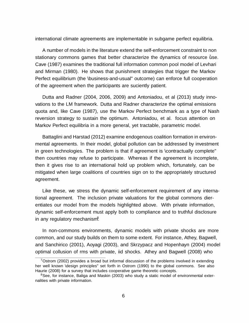
Figure 1: First Best Extraction Rates

Notice that the quota allocated to each country declines or increases over time,

depending on whether the stock is exhaustible (γ ≤ 1) or renewable (γ > 1). No-

tice also that both the rate and the level in (10) are increasing in one’s own re-

source type θi but decreasing in the cross-country average Θ/n. Hence, countries

with larger-than-average carbon usage intensity can extract more. Put another way,

“pro-consumption” types should extract more while “pro-conservation” types should

extract less.

3.5 Implementing the Optimal Quota

As for Step 2, compliance with the first best quota is not automatic. One could

compare the IA’s Euler equation to that of each individual country. That latter

corresponds to a country’s individual incentives for resource consumption, and is

given by:20

θi(1− Et)eit

− (1− θi) = δγ + δγ

(θi(1− Et+1)

ei t+1

− (1− θi)).

20The derivation mirrors the algorithm for solving the planner’s problem in Appendix 7.1.

14

As before, the forward solution is easily found.

(11)(1− Et)eit

=δγ

θi(1− δγ)+

1− θiθi

From (11), one can calculate country’s best response to the extraction rates E−itof other countries:

(12) eit = BRi(θi, E−it) = θi(1− δγ)(1− E−it)

Predictably, pro-extraction types have a greater incentive to extract more. It is easy

to verify that BRi(θi, E∗−i t) > e∗i . In other words, the individual country’s incentives

are toward greater extraction than that prescribed by the IA.21

Consequently, the quota system described by (10) is the optimal one only if it can

be implemented by a SPE (Step 2 in the solution algorithm). This is summarized in

the following result.

Proposition 1 (Full Information Benchmark) Consider the model with full in-

formation satisfying δγ < 1. Then the IA’s optimal quota system (the solution to

(5) ) is the quota system c∗(θ) described by (10). Namely,

(13) c∗it(θ) =θi(1− δγ)

nωγ

t

0

(1− Θ(1− δγ)

n

)γ(1−γt)/(1−γ)

∀ i ∀ θ ∀ t

Proposition 1 is a useful benchmark for comparing subsequent results with private

information. Note that the implementation result holds for any discount factor δ > 0,

including impatient ones. This is possible because payoffs are unbounded below,

reflecting the idea that in a global commons, the costs of full resource depletion may

be catastrophic.

As a consequence, the IA can recommend further threats of resource depletion in

any continuation payoff, even ones that are already punitive, to enforce compliance.

Since increased resource depletion hurts all countries, the credibility of the punishment

21Note that solving (12) as a simultaneous system of equations across countries yields the uniqueMarkov Perfect equilibrium (MPE) — the analogue of the “business-as-usual equilibrium” computedby Cave and by Dutta and Radner in their models. The analytical solution to the MPE in the presentmodel is worked out in Harrison and Lagunoff (2015, Sect. 4).

15

depends on even harsher punishment if the countries fail to carry out the sanction.

This means, in turn, that increasingly severe depletion threats must be used, each

such threat made credible only by even more severe depletion threats later on, and so

forth. The successive threats are only reached, of course, by further deviations at each

counterfactual stage. Since each country’s payoff in the residual stock is unbounded,

the sequence of threats can be recursively defined. The proof in the Appendix gives

the formal details.

Further, the equilibrium does not actually require monitoring by the IA, since

the punishments at each counterfactual stage are not tailored to the perpetrator who

deviated from the prescribed rate. Instead, it need only monitor the aggregate stock

itself to determine whether a deviation occurred.

Finally, we emphasize that the algorithm for constructing punishments is not

sensitive to the location of the social optimum. Indeed, because the punishments are

potentially unbounded, any finite payoff profile can be implemented in this way.

3.6 Credibility of the Implementation

Given the construction, a few questions naturally arise. First, does implementation

works in a commons model for any flow payoff that diverges to −∞ as Et → 1? The

proof in the Appendix indicates the answer is yes, although we do not offer an explicit

proof of the general case.

Second, is it credible for the IA to carry out draconian punishments in the event of

repeated violation? One can argue this both ways. We point out that the IA here is

merely a coordination device — it has no enforcement powers. Thus the punishments

are self-enforcing, carried out as they are by the participants, and sustained by the

self-fulfilling expectations of others’ behavior. In this sense, the international agency

need not be credible in order for the implementation to work.

Third, how would implementation proceed if unbounded punishments were not

permissible or feasible? The most direct alternative to the present construction is a

Markov Perfect reversion strategy. The idea is straightforward. If a country defects

from the optimal quota, then all countries revert to a Markov Perfect Equilibrium

from that period forward. The deterrent works if the participants are patient enough.

16

This type of implementation is described in Cave (1987), Dutta and Radner (2006),

and in a more closely related model of ours (Harrison and Lagunoff (2015), Section 4).

Significantly, even when participants are patient, the reversion strategy only works if

the participants are not too heterogeneous.22

4 Persistent Private Shocks

This Section investigates the nature of optimal quotas when each country’s internal

costs and benefits of resource usage are privately observed as countries are hit with

idiosyncratic private shocks.

The shocks capture a degree of unpredictability of the effect of climatic change

within each country. Moreover, country’s resource shock is assumed to be observable

only to that country, presuming that countries have inside knowledge of changing

business conditions and “local inventories” of sources and sinks of GHG.

Consider a scenario, for instance, in which a warmer climate lowers a country’s

agricultural yields. This, in turn, leads to more intense use of petroleum-based fer-

tilizer, thus increasing the country’s relative value of carbon. In another scenario,

the warmer climate leads to an increase in the saline contamination of the country’s

fresh water fisheries. In that case, the relative value of carbon decreases as GHG

costs increase. The international agency is keen to know which scenario prevails,

but must rely on self-reported information by the countries, a fact explicitly recog-

nized in many international agreements. See, for instance, Article 12 under the UN

Framework Convention for Climate Change, and Articles 5 and 7 under the Kyoto

Protocol.

The shock is assumed to hit i’s type at t = 0. One natural interpretation is

that this is the limiting case of a more general scenario in which each country incurs

serially correlated private shocks to its resource type each period. The present model

corresponds to the case in which shocks are perfectly persistent.23 Perfect persistence

is a reasonable approximation to a situation where environmental change is more

22The problem is that if a country’s type θi is too low, then it may prefer the MPE over a planner’ssolution with equal welfare weights.

23An external appendix explore the general case and extends our main result (Proposition 2) tothis case. See faculty.georgetown.edu/lagunofr/optimal-resource10-External-Appendix2.pdf.

17

rapid than technological progress.

Country i’s type θi is therefore determined by a distribution Fi(θi). For simplic-

ity we analyze a symmetric situation in which Fi = Fj for all i and j. Under the

production interpretation of the model the shocks to types represent exogenous tech-

nological change. We assume the shocks are independent across countries, with Fi(·)differentiable in θi, has full support on [θ, θ], and admits a continuous density fi(·).The distribution Fi is assumed to be commonly known to all countries, however, each

country’s realized shock each period is privately observed.

4.1 Optimal Quota Systems with Private Shocks

As before, the international agency (IA) recommends a quota system. To make an

effective recommendation, the international agency is a gatherer and dispenser of

information. The IA solicits information concerning each country’s realized type θi.

As before, the IA is a weak mechanism designer. It cannot compel the countries to

report truthfully. Nor can it withhold information since the revelation of information

by each country is public. Instead, the IA serves only as a vehicle for coordinating

information and usage. Again, this is appropriate in the international setting where

there is no global government with external enforcement capability.

Each member country chooses whether or not to disclose its type (as, for instance,

when countries make public their national income accounts, estimates, and forecasts).

A country’s reported type is denoted by θi. The entire profile of types reported by

all countries is θ = (θ1, . . . , θn).

A quota system then conditions on the reported profile θ. To distinguish this from

the full information case, we denote a quota system here by c◦. Formally, a quota

system is given by the sequence c◦ = {c◦t (θ)}, t = 0, 1, . . ..

To obtain the desired quota system, the IA recommends both a usage and a dis-

closure strategy. Formally, a disclosure strategy for country i is map µi(θi) describing

i’s report at the beginning of t = 0 after realizing its type.

A usage strategy now is a map σi(ht, θ, θi) = cit determining i’s consumption at

date t given the extraction history, the disclosure profile, and its resource type.

18

To an extent, the disclosure mechanism resembles some existing protocols. Arti-

cle 12 of the UN Framework Convention on Climate Change, for instance, requires

its signatories to periodically submit, among other things, a “national inventory of

anthropogenic emissions,” and a “specific estimate of the effects that the policies and

measures ... will have on anthropogenic emissions by its sources and removals by its

sinks of greenhouse gases...”

Let µ = (µ1, . . . , µn) and σ = (σ1, . . . , σn) denote profiles of disclosure and re-

source usage, resp., and after any history, let µ(θi) = (µi(θi))ni=1 and σ(ht, θ, θ) =

(σi(ht, θ, θi))

ni=1. Given a strategy pair (σ, µ), the long run expected payoff to a coun-

try i at the resource consumption stage in date t is

(14)

Vi(ht, θ, σ, µ| θi) ≡

∫θ−i

[θi log σi(h

t, θ, θi) + (1− θi) log(ωt −n∑j=1

σj(ht, θ, θj) )

+ δVi(ht+1, θ, σ, µ| θi)

]dF ◦−i(θ−i| ht, θ)

where F ◦−i(θ−i| ht, θ) will denote the posterior update about other countries’ resource

types when ht is the usage history, θ is the disclosure profile, and (implicitly) given

the strategy pair (σ, µ).

At the disclosure stage, country i’s interim payoff before observing the disclosed

type of others is ∫θ−i

Vi(h0, µ(θ), σ, µ| θi)dF−i(θ−i).

To implement a quota system, the IA recommends a profile (µ, σ) of disclosure and

usage strategies. Each period it solicits information from each country about its type.

If these prescriptions are followed, then all countries disclose their types according

to µ. The IA then makes public the reported profile θ. We focus on truth-telling

disclosure strategies, i.e., those in which µ prescribes θi = θi for each country.

The strategy pair (µ, σ) with truth-telling disclosure may then be said to imple-

ment the quota system c◦ in the private shocks model if (µ, σ) yields c◦ along the

outcome path.24

24As with the full information case, the consumption path is generated recursively: c◦0(θ) =σ(h0, θ, θ), then c◦1(θ) = σ(h1, θ), where h1 = (h0, σ(h0, θ, θ), (ω0 − C0(θ))γ ), etc.

19

A quota system is feasible only if it can be implemented by, a Perfect Bayesian

equilibrium strategy pair (σ, µ). The pair (µ, σ) and a belief system F ◦i (θi| ht, θ), i =

1, . . . n constitute a Perfect Bayesian equilibrium (PBE) if (i) at the consumption

stage in date t, σi and µi together maximize i’s long run expected payoff (defined in

(14)) given usage history ht, disclosure profile θ, i’s type θi, and given the strategies of

other countries; (ii) at the disclosure stage, σi and µi together maximize i’s expected

payoff given ht, given θi, and given the strategies of others; and (iii) beliefs F ◦ satisfy

Bayes’ Rule wherever possible.

Note that at the disclosure stage, countries contemplate disclosure deviations from

the prescribed plan, taking account of the fact that they have the freedom to deviate

in their extraction plans at a subsequent stage. This potential for “thoughtful” devi-

ations limits the types of punishments that any IA can suggest to the members. This

also complicates the members’ beliefs off-path. After any deviation from prescribed

usage strategies, other countries must determine what type of deviation — a resource

use deviation, or an earlier disclosure deviation, or both — occurred.

If, however, (σ, µ) is a truth-telling PBE that implements c◦, then along the

equilibrium path, the realized payoff for i following any type history θt satisfies

(15) Vi(ht, θ, σ, µ| θi) = Ui(ωt, c

◦(θ), θi)

Consequently, the IA will recommend a quota system c◦ and a PBE (σ, µ) that

solves

(16)

maxc◦

∑i

∫θ

Ui(ω0, c◦(θ), θi)dF (θ) subject to c◦ implemented by the PBE (σ, µ).

Any quota that solves (16) will be called an optimal quota. Our main result is that

the optimal quota has a special form which we refer to as fully compressed. A quota

system c◦ is fully compressed if for every country i, the recommended quota c◦it for

country i at date t does not vary with the realized profile of shocks θ. In other words,

the quota is completely insensitive to the countries’ realized preferences/ production

intensities for carbon.

20

4.2 A Full Compression Result

For the result below, one further assumption is required:

Dispersion Restriction. The parameters n, δ, γ, and θ jointly satisfy θ > 11+(n−1)δγ

.

The dispersion restriction is a weak condition that bounds the relative dispersion

of types by the discounted number of participants.25 In general the larger the global

commons problem (the larger is n), the more dispersed the resource types can be and

still satisfy the constraint.

Proposition 2 Consider the model with private, perfectly persistent shocks such that

the dispersion restriction is satisfied. Then the optimal quota c◦ (the solution to (16))

is fully compressed. Specifically,

(1) the extraction rates corresponding to c◦ are stationary, fully compressed, and

given by:

(17) e◦i =(1− δγ)

[∫ θθθidFi(θi)

]n

for each country i.

(2) c◦ is implementable by an equilibrium in which each country’s prescribed extrac-

tion rate after any history is stationary and fully compressed.

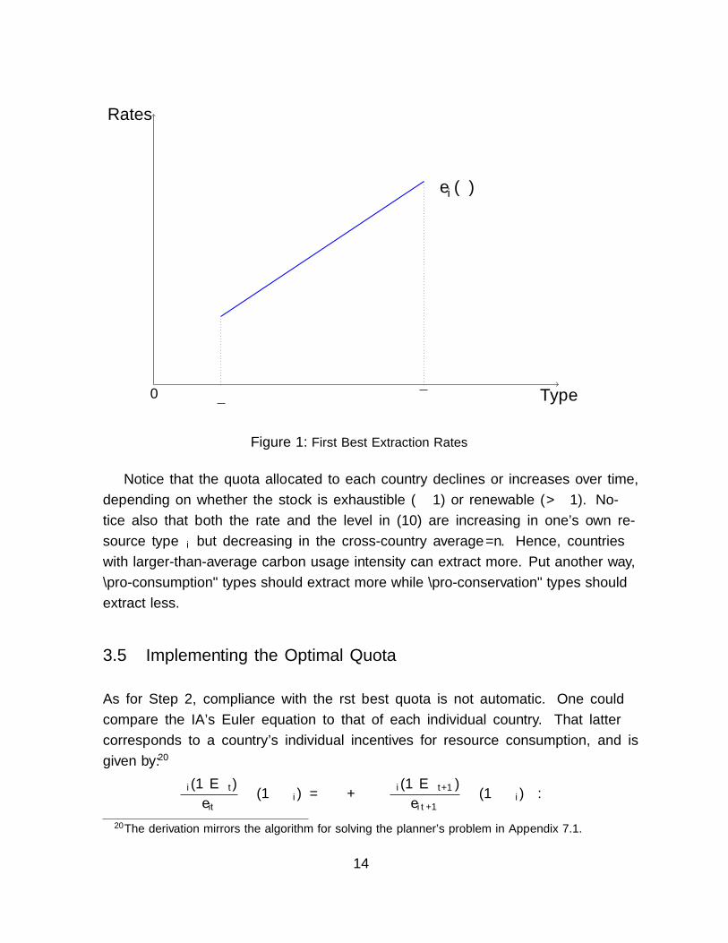
To illustrate what compression means for the optimal quota, compare the optimal

rate e◦ in (17) to the full information solution in (9). This is illustrated in Figure

2. Under private shocks, the optimal quota assigns all countries identical extraction

rates, despite the fact that the international agency can condition its recommendation

on the information disclosed by each of the countries (again see Figure 2). If, for

instance, Fi is uniform on [θ, θ], then in the optimal quota, all countries are required

25To illustrate just how weak it is, consider δγ = .8 and n = 193 (the number of countries in theU.N.). Then the lower bound θ need only exceed .0065 (approximately) to satisfy the dispersionconstraint. To take an even more pessimistic case, consider δγ = .5 and n = 34 (the number ofcounties in the OECD). Then the dispersion constraint is satisfied when θ > .0571.

21

Type0 θ θ

Rates

e∗i (θ) (full information)

e◦i (private shocks)

Figure 2: Optimal quota: Private Shocks vs Full Information

to extract resources at the same rate e◦i = (1−δγ)(θ+θ)/2n, even if they realize very

different resource types.

Proposition 2 has troubling implications for any prospective climate agreement.

Countries with realized usage values above the mean must extract less than under

the full information optimum. Those below the mean can extract more (Fig. 2).

Generally, the informational rents accorded to low types gives them considerable

“bargaining power.” Relative to the full information optimum, high types subsidize

low types. In concrete terms, it suggests that fast-developing countries with higher

than expected resource demand (India, Brazil, and China) must, in a sense, subsidize

countries with lower than expected resource demand (U.S., Japan, EU countries).

Moreover, the compression holds even if private information on the country shocks

is negligible. To see this, fix any ε-neighborhood of a particular type θ ∈ [θ, θ] and

consider a distribution Fi that places all but ε of its mass on that neighborhood while

maintaining full support. Observe then that Proposition 2 holds for any ε > 0.

It is worth noting that while the Proposition describes the optimal quota by its

22

extraction rates, one can characterize the optimal consumption profile by

(18) c◦it(θ) =(1− δγ)

∫ θθθidFi(θi)

nωγ

t

0

1−(1− δγ)

∑i

∫ θθθidFi(θi)

n

γ(1−γt)/(1−γ)

for each country i and each date t. Here, consumption is not stationary but it is

compressed. Consumption may grow or contract over time depending on whether the

depletion rate γ admits growth.

Before proceeding with the logic of Proposition 2, we consider what the planner

would choose if it never observed the realized types. In that case, the optimal

mechanism is, of course, compressed and coincides with the compressed mechanism

in the Proposition.

5 The Logic of Full Compression

5.1 Intuition from first order conditions

This section illustrates the basic logic of the result.26 The proof proceeds by first

introducing a “relaxed planner’s problem” similar to the one in the full information

benchmark. In this case, the PBE constraint in the relaxed problem is replaced by

a weaker constraint that requires only truthful disclosure. Compliance incentives

following disclosure are ignored. The International Agency then faces only a single

disclosure stage at the beginning of t = 0 (since compliance is ignored). This is given

by the truth-telling constraint:

(19)

∫θ−i

Ui(ω, c◦(θ), θi)dF−i ≥

∫θ−i

Ui(ω, c◦(θi, θ−i), θi)dF−i ∀θi ∀θi

The “relaxed planner’s problem” is stated as

(20) maxc◦

∑i

∫θ

Ui(ω, c◦(θ), θi)dF (θ) subject to (19).

To understand the argument, we consider, as a solution to the relaxed problem,

an extraction plan c◦ that is both stationary and symmetric. This is later established

in the proof. For now, these properties are taken as given.

26A more detailed outline of the proof is given in Section 7.3.1.

23

To show how non-compression is ruled out, observe that for any profile θ−i of

others’ types, the full information optimal extraction rate for country i possessing

the highest type θ is

e∗i (θ, θ−i) = e ≡ θ(1− δγ)/n.

This extraction rate serves as a cutoff. The proof shows that solution to the indirect

problem must be consistent with an extraction plan e◦i (θ) for each i that lies below

e. By contrast, under the Dispersion restriction, if a type could freely choose its

extraction rate ei then it would choose a larger extraction rate than e. This is shown

formally in the proof, but can be illustrated heuristically using first order conditions.

First, rewrite the payoffs. One can verify that under any stationary plan, country

i’s payoff in the relaxed problem may be expressed as

(21) Ui(ω0, c◦(θ), θi) = k0 + k1 log(1− E◦(θ)) − θik2 log

(1− E◦(θ)e◦i (θ)

)where e◦ is the stationary extraction rate corresponding to c◦, and k0, k1, k2 are

positive constants given by

(22) k0 =logω0

1− δγ, k1 =

∞∑t=0

δtt∑

j=0

γt−j, and k2 =1

1− δ

We illustrate why separating equilibria cannot arise in the case where extraction

plan e◦i for country i is differentiable in θi on some subinterval Θi ⊆ [θ, θ]. Using (21),

the interim payoff to type is θi is

k0 +

∫θ−i

(k1 log(1− E◦(θ)) − θik2 log

(1− E◦(θ)e◦i (θ)

))dF−i(θ−i)

Consequently, the incentive constraint for an interior type θi ∈ Θi satisfies the first

order condition, ∫θ−i

[k2θie◦(θ)

− k1 − k2θi1− E◦(θ)

]∂e◦i (θ)

∂θidF−i(θ−i) = 0

If e◦ is fully compressed, then∂e◦i (θ)

∂θi= 0 and the first order condition is trivially

satisfied. Suppose that for some type θi, the set Θ−i(θi) ≡ {θ−i :∂e◦i (θ)

∂θi6= 0} has

F−i-positive probability. Then the first order condition becomes∫θ−i∈Θ−i

[k2θie◦(θ)

− k1 − k2θi1− E◦(θ)

]∂e◦i (θ)

∂θidF−i(θ−i) = 0

24

One can contrast this with first order condition for i’s best response, call it eBi , to

the relaxed solution e◦−i under full information:

k2θieBi (θ)

− k1 − k2θi1− E◦−i(θ)− eBi (θ)

= 0 ∀ θ.

We can then use the dispersion restriction to show that any solution e◦ to the

relaxed problem satisfies e◦i (θ) < eBi (θ) for each i and almost every θ. In other words,

if it were possible for a country to freely choose its extraction rate ei, it would opt

for one larger than allowed by the relaxed optimal quota, regardless of the realized θ.

From this free rider problem, it follows that

k2θie◦i (θ)

− k1 − k2θi1− E◦(θ)

> 0 ∀ θ.

Hence, if∂e◦i (θ)

∂θi> 0 for almost all θ−i ∈ Θ−i then the first order condition for incentive

compatibility will be violated.

To summarize, if e◦ is not compressed, then a country can move closer to its

preferred extraction rate, not by cheating on the quota, but rather by misreporting

its type. It will mimic a type that is allotted a higher extraction quota.

Naturally, this is a heuristic argument. It suggests that any optimal extraction

plan must be compressed locally but does not rule out, for instance, step functions.

It nevertheless suggests a broader intuition. Namely, a free rider problem will

exist with any solution to the planner’s problem. Because of the “complementarity”

between a country’s actions and its reports, if any solution were non-compressed then

a country can move closer to its preferred extraction rate by manipulating its report.

The planner has no additional instrument to offset to this incentive to manipulate.

The planner’s only instrument is e and so full compression cannot be avoided.

5.2 Transferable Utility and Side Payments

In contrast with the logic above, environments with transferable utility provide to the

planner an additional instrument — side payments. In the literature on self-enforcing

environmental agreements (absent private information) the inclusion of monetary

25

transfers or side payments in a climate agreement is often referred to as issue linkage

(see Finus (2001)).

The transferable utility (TU) model provides a stark contrast with the full com-

pression result. Using the expression for payoffs in (21) consider the following variant

of the model: after receiving a reported profile, the planner can divide up the constant

amount nk0 = n logω0

1−δγ and allocate it to the countries according to some formula. The

allotment can include both positive (transfers) and negative values (taxes), depend-

ing on the reported profile. This allotment constitutes a transferable utility payment

to/from each country.

Formally, let si(θ) denote a tax/transfer from/to country i given the reported

profile θ. One can have either si(θ) > 0 or si(θ) < 0. A balanced transfer scheme

satisfies∑

i si(θ) = nk0 for every profile θ (where k0 is defined in (22) ). With this

transfer, the country’s payoff under truth-telling is

(23) Ui = si(θ) + k1 log(1− E◦(θ)) − θik2 log

(1− E◦(θ)e◦i (θ)

).

Comparing (23) with the no-transfer payoff in Equation (21), we see that the constant

k0 is replaced with a type-contingent transfer si(θ).

Proposition 3 There exists a PBE with a balanced transfer scheme s = (s1, . . . , sn)

that implements the first-best (full information optimal) quota c∗(θ).

Proposition 3 indicates that when the payoffs admit a TU representation, then the

previous result is reversed and the first best is implementable.

Compression in the original model occurs precisely because each of the separable

components of the payoffs are either independent of θ — as is the case with k0 —

or they jointly depend on θ via the extraction profile e◦. By contrast, transferable

utility imparts a degree of freedom to the planner by adding a linear type-contingent

payoff that does not depend directly on e◦.

The proof in the Appendix constructs a transfer scheme that adapts a well-known

result of d’Aspremont and Gerard-Varet (1979) to the present model. In this con-

26

struction, the transfer to country i is

(24)

si(θi, θ−i) = k0 +

∫θ−i

∑j 6=i

[Uj(ω0, c◦(θi, θ−i), θj)] dF−i

− 1

n− 1

∑j 6=i

∫θ−j

∑k 6=j

[Uk(ω0, c◦(θ), θk)] dF−j

In this construction, the average transfer is k0 = logω0

1−δγ > 0. Hence, on average,

countries receive the value k0 of accumulated resource stock just as they did without

the transfer. In relative terms, however, high type realizations are penalized, receiving

a lower value than k0. Meanwhile, low types receive a higher value than k0. When

aggregated over all countries, the transfers sum to nk0.

In the Appendix proof, we verify that i’s transfer depends only payoffs of other

countries, and an aggregated part that integrates out i’s type. By turning what

previously was a constant term into a type contingent one, si aligns the payoff of i

with those of the planner. Consequently, i has no incentive to lie. Note that the

payments do not affect incentives at the compliance stage, and so the compliance

arguments are unaffected.

The addition of transferable utility to our model is not simply a relaxation of an

institutional constraint (i.e. “forbidding” side payments between countries), but is

rather a fundamental change in the payoffs of each country’s representative citizen.

It is an open question whether and to what extent transfers can improve things under

non-transferable utility (NTU) — as is the case in the present model. For a number

of reasons, NTU transfers are problematic in our framework. First, the common NTU

unit of account here is a resource unit such as carbon. The designer could conceivably

propose an emissions trading system. Given the Revelation Principle, however, any

trading mechanism that the designer could propose would be a special case of a quota

system as defined already.27

Second, the direction of transfer indicated in (24) is regressive. To improve wel-

fare, the scheme will at some point involve transfers from poor countries to rich ones.

Specifically, in order to counteract compression, countries that realize shocks with

high usage value (relative to its value of conservation) would be required to subsidize

27NTU transfers in other dimensions include non-climate benefits, technology transfers, tradeterms, etc. To add these would require a substantially richer and higher dimensional model, but aworthwhile extension.

27

those with low usage value. Yet, the large projected increase in usage by developing

countries, coupled with per capita reductions in GHG production by wealthier coun-

tries, means that relatively poorer countries will eventually be the ones with high

usage value.28

Finally, the presence of side payments or any other form of issue linkage com-

pounds transaction costs of reaching a global agreement. Along this line of argument

Calcott and Petkov (2012) shows how cross-country heterogeneity reduces the possi-

bility of an efficient implementation of transfers. They model the case of heteroge-

neous countries, under full information, focusing on transfers that are time invariant,

linear in emissions, and consistent with budget balance. They find that heterogeneity

reduces the scope for penalty schemes to jointly satisfy desirable emissions reduction.

5.3 Robustness Issues

Credibility. As with the compliance scheme in the full information environment,

one can ask whether a planner will carry out the disclosure rule. At first glance,

this may seem problematic. Consider, for instance, a truth-telling equilibrium that

implements the optimal quota. Since the quota is fully compressed, each country has

no incentive to lie about its type in date t = 0. This means that the IA now has

full information about countries’ types heading into date t = 1. Without the ability

to commit to a mechanism at t = 0 the IA would make use of this information to

implement the first-best solution in date t = 1 and beyond. However, this destroys

the initial incentive for truthful disclosure.29

Consequently, if the IA can re-optimize at any date, then the equilibrium must be

constructed so that disclosure strategies are pooling. Fortunately, this is easily done

since the mechanism is already known to be fully compressed both on and off path.

Commons versus Market Incentives. One can also ask why the full compression

holds in the commons environment but not necessarily in market frameworks. The

countries in this environment can be compared to seller’s in a procurement auction,

28See projected usage estimates from the Carbon Dioxide Information Analysis Center (CDIAC),cdiac.ornl.gov.

29This “ratchet effect” was originally observed by Roberts (1984) in a dynamic Mirleesian modelof optimal taxation.

28

each attempting to bid for the right to emit carbon. A few key differences arise. In

a standard auction or oligopoly there are trade offs in the production quota between

seller types. An increase in the market share for a type θi, for instance, must be

compensated by either a reduction in the share given to another seller-type on average.

Given the hard trade offs in these cases, productive efficiency will usually require that

the quota prescribe different levels for different seller types. For this reason, optimal

mechanisms will not generally be compressed.30

One exception to the “un-compressed” optimal mechanism occurs when hazard

rates Fi/fi are strictly increasing. In that case, the loss from inefficient production is

offset by allocative concerns of the planner. Athey and Bagwell (2008) for instance,

analyze a repeated oligopoly setting in which firms receive serially correlated cost

shocks each period. They show that the optimal production quota for colluding firms

is fully compressed (which they refer to as “rigid”) when either hazard rates are

increasing or the maximum possible compensation from monopoly pricing is large

enough.

McAfee and McMillan (1992) show a similar result when buyers collude in a static

procurement auction under free entry. Finally, Lewis (1996) argues that compression

would occur naturally when government uses standard policy instruments to regu-

late environmental externalities in a perfectly competitive static environment with

privately observed costs and benefits of pollution. He shows, however, that without

constraints on the instrument, the incentive-efficient mechanism is not compressed.

These results depend critically on the fact that market shares are bounded and

in fact add up to one. This means that there are one-for-one trade offs across types

in the oligopoly framework. By contrast, there is no such aggregate constraint in

the global commons framework. The stored resource ωt is non-rivalrous, and so all

countries’ values for, say, carbon storage can be increased simultaneously by simply

withholding carbon consumption. For these reasons, the results from oligopolies (or

procurement auctions) cannot be applied to the present model.

Imperfect Persistence. The compression result can be extended to a more general

model of imperfect persistence. Specifically, a country is hit with a shock to its

30See Pavan, Segal, and Toikka (2012) for a comprehensive characterization of optimal mechanismsin Markov models of private information.

29

resource type each period according to a stationary Markov process. If that process

is a martingale, then the quota will remain compressed.

Hence, two countries that start identically will typically evolve very different ben-

efits and costs of resource use. They are, nevertheless, prescribed the same con-

sumption quota throughout. The extension and result is described in an external

appendix.31

The Parametric Structure. Finally, one can ask whether the results hold under

a more general parametric setup. As a general matter, one can only speculate. Here

we examine a generalization based on a utility function adapted from Antoniadou

et al. (2013) (the “AKM model” from here on).32 We extend the AKM model to

a heterogeneous agent environment, and in an external appendix derive the Euler

equations for the full information case.33

The law of motion in AKM model is given by

(25) ωt+1 =[γ(ωt − Ct)1− 1

η + (1− γ)φ1− 1η

] ηη−1

where η > 0. The larger is the second term in [·] the lower is the incremental effect

of current resource depletion on future stock.

Now consider a flow utility for country i of

(26) ui = θic1− 1

η

it − 1

1− 1η

+ (1− θi)(ωt − Ct)1− 1

η − 1

1− 1η

.

The flow payoff in AKM model corresponds to Equation (26) in the special case where

θ = 1. Equation (26) simultaneously varies the elasticity of substitution η between

extraction and preservation and the relative payoff weights given to each in ui.

Notice that when taking the limits η → 1, γ → 1, and setting φ = 1, Equations

(25) and (26) converge to Equations (1) and (2), respectively. Hence this model is a

generalization of our benchmark model.

31The argument is largely based on the proof of Proposition 2. It combines Part 1 of the originalresult, the martingale assumption which allows one to apply recursive logic. The proof of compliancemimics the steps of the proof of Proposition 2 (part 2). See faculty.georgetown.edu/lagunofr/optimal-resource10-External-Appendix2.pdf for the formulation and details.

32We thank a referee for suggesting the extension.33The external appendix can be found on faculty.georgetown.edu/lagunofr/optimal-resource10-

External-Appendix1.pdf.

30

For this more general model, the external appendix displays the Euler equations

for the full information case.34 We verify that the planner’s problem is stationary, but

does not admit an explicit solution. It turns out that the implementation in Propo-

sition 1 holds when the CES parameter is in the set (0, 1), but not when it is greater

than 1. Basically, payoffs are bounded in extension when η ≥ 1. But the construction

of punishments in Proposition 1 applies only to commons problems in which payoffs

are unbounded below. When payoffs are bounded, and an alternative construction of

punishments, based on a Nash reversion strategy is worked out in Harrison and La-

gunoff (2016). They show, however, the reversion strategies implements the optimum

only for certain parameters.

It is unclear whether Proposition 2 can be extended to this case. Future research,

making use of computational methods, would help to resolve this question.

6 Conclusion

This paper studies dynamic mechanisms for global commons with environmental ex-

ternalities. Using carbon consumption as the leading example, we generalize the

dynamic resource extraction game of Levhari and Mirman (1980) to allow for direct,

heterogeneous benefits of resource conservation across countries. We examine the

case where countries incur payoff/technology shocks. These shocks alter the way that

countries evaluate the relative benefits and costs of carbon consumption over time.

An optimal quota system is an international agreement that assigns emissions

restrictions to each country as a function of the sequence of realized type profiles

such that it be implementable in PBE. The PBE builds in the idea of sequential

self-enforcement in both compliance and disclosure.

Our main result is that the optimal quota system is fully compressed. The result is

stark, as it suggests that the quota can only be tailored to ex ante differences between

countries. Among other things, it should not vary with the realized evolution of a

country’s climate costs or its resource needs.

34These set of equations, beside helping to study the robustness of our results, can be helpful asa new baseline model with which to explore other issues in resource dynamics.

31

The results stand in contrast to with many actual international proposals (see

Bodansky (2004) for a survey). Most of these advocate maximal flexibility in making

adjustments particular characteristics of each country. Article 4 in the UNFCCC

explicitly references the need to account for “the differences in these Parties’ starting

points and approaches, economic structures and resource bases, the need to maintain

strong and sustainable economic growth, available technologies and other individual

circumstances, as well as the need for equitable and appropriate contributions by each

of these Parties to the global effort ...”

The results may be reconciled to these approaches to the extent that transfers can

be used, or that some information about local shocks is globally observed. Indeed,

our study suggests a critical role for sided payments, although not, as many policy

makers suggest, for purposes of distributive justice (again see Bodansky (2004)). Both

distributive concerns and political economy constraints may limit or negate the sorts

of transfers or side payments needed to overcome the information frictions of the type

we model.

As for increased information, inefficient compression could be mitigated if the

data gathering process occurs above and beyond the reach of sovereign filters. This

is an important consideration for the climate science itself. As before, any mitigating

mechanism based on globally public information must be self enforcing at compliance

stage or should be enforceable by the International agent. In our view, the disclosure

of country-specific observations of economic costs and benefits remains problematic

because these costs and benefits rely heavily on each country’s yearly disclosure of its

national income accounts. Public provision of “investigative” resources to generate

such information, however, might overcome this problem. It seems an excellent topic

for future study.

7 Appendix: Proofs of the Results

7.1 Derivation of Planner’s Solution

.

32

Starting from the Euler equation

θieit−

n∑j=1

(1− θj)(1− Et)

+n∑j=1

δ[∂Uj(ωt+1, e,θj)

∂ωt+1

∂ωt+1

∂eit] = 0

with∂ωt+1

∂eit= −γωγt (1− Et)γ−1, then the first order condition becomes

(27)θieit−

n∑j=1

(1− θj)(1− Et)

= γδn∑j=1

[∂Uj(ωt+1, e,θj t+1)

∂ωt+1

ωγt (1− Et)γ−1]

Differentiating the value function Uj(ωt+1, e,θj) with respect to ωt+1 yields,

∂Uj(ωt+1, e,θj)

∂ωt+1

=1

ωt+1

+ δγ∂Uj(ωt+2, e,θj)

∂ωt+2

ωγ−1t+1 (1− Et+1)γ

Substituting this into the first order condition, we obtain

θieit−

n∑j=1

(1− θj)(1− Et)

= δγn∑j=1

{1

ωt+1

+∂Uj(ωt+2, e,θj)

∂ωt+2

ωγ−1t+1 (1− Et+1)γωγt (1− Et)γ−1

}=

1

1− Etγδ

n∑j=1

{ωγt (1− Et)γ

ωt+1

+∂Uj(ωt+2, e,θj)

∂ωt+2

ωγ−1t+1 (1− Et+1)γωγt (1− Et)γ

}=

1

1− Et

(nδγ + δγ

n∑j=1

∂Uj(ωt+2, e,θj)

∂ωt+2

ωγt+1(1− Et+1)γ

)

=1

1− Et

(nδγ + δγ

n∑j=1

[(θj(1− Et+1)

ej t+1

−n∑j=1

(1− θj))]

)

Reorganizing terms, we obtain

(28)θi(1− Et)

eit−

n∑j=1

(1− θj) = nδγ + δγ

[θi(1− Et+1)

ei t+1

−n∑j=1

(1− θj)

]

which is Equation (7) in the main body of the paper.

Define sit ≡ θi(1−Et)eit

−∑n

j=1(1− θjt). Then

sit(θi) = nδγ + δγsi t+1(θi).

33

Forward iteration yields a steady state sit = nδγ(1−δγ)

and plugging in the last equation

we obtainθi(1− Et)

eit−

n∑j=1

(1− θj) =nδγ

(1− δγ).

Then:

θi(1− Et)eit

−n∑j=1

(1− θj) =nδγ

(1− δγ)(29)

θi(1− Et)(1− δγ)− eit∑j

(1− θj)(1− γδ) = eitγδn

θi(1− Et)(1− γδ)− eit(n−∑j

θj)(1− γδ) = eitγδn(30) ∑j

θj(1− Et)(1− γδ)− (1− γδ)Et(n−∑j

θj)− Etγδn = 0(31) ∑j

θj − nEt −∑j

θjγδ = 0(32)

using Equations (29)-(32) we get

(33) e∗i (θi) =θi(1− δγ)

n

which is equivalent to Equation (9) in the main text.

7.2 Proof of Proposition 1

Fix a profile θ. As we have already shown that c∗(θ) maximizes∑

i Ui without the

equilibrium constraint, it remains to show that c∗(θ) can be implemented by a SPE.

For ease of exposition, we will work with extraction rates ei rather than levels ci.

To prove the result, we will construct a sequence {eτ (θ)}∞τ=0 of extraction profiles,

and a strategy profile σ satisfying for each i:

(i) σi(h0, θ) = ω0e

0i (θ),

34

(ii) for each τ ≥ 0 and each t ≥ τ , if ht(eτ (θ)) represents history in which some

country deviated unilaterally from profile eτ (θ) in date t− 1, then set

σi(ht(eτ (θ)), θ) = ωte

τ+1i (θ)

(i) For all other histories ht let σi(ht, θ) = ω0e

0i (θ).

Our task is to construct the sequence {eτ (θ)}∞τ=0 in such a way that σ is a SPE,

i.e., Vi(ht, σ, θ) ≥ Vi(h

t, σi, σ−i, θ) for all i, all σi, and all histories ht, and along the

equilibrium path h∗t at date t, σi(h∗t, θ) = c∗it(θ).

Our sequence is constructed recursively as follows. Starting from ω0, for any

stationary dynamic path e of usage rates, the long run payoff to a country i can be

expressed as

(34)

log(ω0)

1− δγ+

∞∑t=0

δt[(

1

1− δγ− θi

)log(1− E) + θi log ei

]≡ log(ω0)

1− δγ+

∞∑t=0

δt ui

Here, ui captures the long run effect on payoffs of the stationary extraction profile

e chosen at each date t. We refer to ui as the flow payoff even though it includes

future as well as present effects of the current profile e through its effect on the

resource stock ωt. The critical feature used in the proof is the fact that each “flow”

payoff ui is unbounded below. In the rest of the proof we make use of this notation

and, moreover, drop the first term log(ω0)1−δγ which will cancel in any comparison with

an alternative long run payoff.

Let e∗(θ) denote the corresponding path of usage rates in the optimal quota c∗(θ).

Recall that e∗i (θ) = θi(1−δγ)n

. Since e∗(θ) is stationary, i.e., e∗t (θ) = e∗t′(θ) for any pair

of dates t and t′, it yields a payoff

(35) V ∗i (θ) ≡ 1

1− δ

[(1

1− δγ− θi

)log(1− E∗(θ)) + θi log e∗i (θ)

]to each country i (and dropping the term log(ω0)

1−δγ ).

Working with rates rather than levels, we construct a recursive sequence of usage

profiles {eτ (θ)}∞τ=0 as follows. Let e0(θ) = e∗(θ) and V 0i (θ) = V ∗i (θ).

35

Next, for τ ≥ 1, let eτ−1(θ) be a profile of extraction rates. The profile eτ (θ) is

defined as follows.

For each τ , all countries choose eτ (θ) (to be defined shortly) for that period. This

yields each country a flow payoff of uτi (θ). After one period, the countries revert

to optimal extraction rates, e0(θ), if there is no subsequent deviation.35 The payoff

V τi (θ) is therefore defined by

V τi (θ) ≡ uτi (θ) + δV 0

i (θ)

Using the definition in (34) of an arbitrary flow payoff, the payoff in state τ is given

by

(36) V τi (θ) =

(1

1− δγ− θi

)log(1− Eτ (θ)) + θi log eτi (θ) + δ V 0

i (θ)

To complete the recursive definition, we need to define eτ (θ). This will be con-

structed to satisfy the incentive constraint in stage τ − 1. Specifically, if it turns out

that a country deviates in state τ − 1 in some period then the countries transition

to the state τ in the following period so that extraction rates in the next period are

given by eτ (θ). Consequently, for each τ ≥ 1, eτ (θ) is defined to satisfy:

(37) V τ−1i (θ) ≥ uτ−1

i (θ) + δV τi (θ)

where uτ−1i (θ) = max

ei

[(1

1− δγ− θi

)log(1− Eτ−1

−i (θ) + ei) + θi log ei

]is i’s flow

payoff if it chooses a best response to eτ−1(θ) in the current period.

Using the definition of V τi in (36), one can show that the incentive constraint (37)

holds if for all i,

(38)

uτ−1i (θ) + δ(1−δ)V 0

i (θ) ≥ uτ−1i (θ)+δ

[(1

1− δγ− θi

)log(1− Eτ (θ)) + θi log eτi (θ)

]Clearly, these inequalities (one for each country) can always be made to hold by

choosing Eτ sufficiently close to one. Note that it will necessarily be the case that

Eτ > Eτ−1.

To summarize, the sequence {eτ (θ)}∞τ=0 is recursively constructed so that for each

eτ−1(θ), eτ (θ) is chosen to satisfy these incentive constraints. Then σ is constructed to

35We thank a referee for suggesting this simplified construction.

36

give precisely eτ (θ) in any period in which a unilateral deviation occurred in eτ−1(θ)

after which point the strategy takes the countries back to e0(θ) = e∗(θ). Multilateral

deviations revert to e0(θ) as well. By construction, the profile is subgame perfect and

implements c∗(θ).

7.3 Proof of Proposition 2

7.3.1 A Basic Outline

Before proceeding, we give a more formal outline of the argument sketched in Section

5.1.

Recalling the discussion in Serction 5.1, the proof of Part 1 proceeds by first

introducing a “relaxed planner’s problem” as shown in Equation (20). Since the

relaxed problem ignores off-path deviations, all the subsequent arguments here refer

to the on-path incentive constraints in (19).

Without the incentive constraint (19), the solution to the relaxed problem in (20)

coincides the with full information extraction plan (Lemma 1 below). With incentive

constraints, the solution to the relaxed problem can be reformulated using standard

Envelope and monotonicity conditions from the theory of optimal auctions (Lemma

2 below).

Both Lemma 1 and Lemma 2 are used in Lemmata 3-6 (in the proof) to rule out

all possible forms of non-compression. The idea is as follows. For any profile θ−i of

others’ types, the full information optimal extraction rate for country i possessing the

highest type θ is

e∗i (θ, θ−i) = e ≡ θ(1− δγ)/n.

This extraction rate serves as a cutoff. Any solution to the indirect problem must be

consistent with an extraction plan e◦i (θ) for each i that lies below e. This is shown

below in Lemma 3.

By contrast, under the Dispersion restriction, if a type could freely choose its

extraction rate ei then it would choose a larger extraction rate than e. This is shown

in Lemma 4.

37

Hence, if e◦ is not compressed, then a country can move closer to its preferred

extraction rate, not by cheating on the quota, but rather by misreporting its type. It

will mimic a type that is allotted a higher extraction quota. This is shown in Lemma

5.

To prove Part 2 of the Proposition, we need to show that the relaxed-optimal

quota can be implemented by a full-blown PBE in which a country’s prescribed usage

rate after any history is stationary and compressed.

To implement the quota e◦ one might think that the IA could simply use the

sanctions constructed in the full information case. That logic (outlined in the proof

of Proposition 1) requires credible punishment at each counterfactual stage depends

on even harsher punishment if the countries fail to carry out the sanction.

When shocks are private, that construction needs modification. In any PBE with

truth-telling at the disclosure stage, the IA takes at face value any disclosed profile,

manipulated or otherwise. Consequently, a country may have an incentive to report

a type consistent with the least punitive punishment which, in turn, may give it the

incentive to violate the quota itself. Notice that this problem arises whenever the

prescribed usage along the punishment path varies across type. So, even though the

quota c◦ itself is compressed, it may be difficult to implement in Perfect Bayesian

equilibria if the sanctions are not. The result in Part 2 by-passes this problem by

showing that the optimal quota can be implemented by compressed sanctions.

7.3.2 The Proof

Part 1. We begin by establishing some facts about the planner’s relaxed problem

in (20).

Lemma 1 The full information solution e∗i (θi) ≡ θi(1 − δγ)/n for country i solves

(20) if the truth-telling constraint (19) is dropped.

Proof of Lemma 1. By dropping the constraint (19), truthful revelation is assumed

to hold at t = 0, and so the planner implements the full information optimum e∗ after

receiving the profile θ. The Lemma therefore follows.

38

Call an extraction plan c◦ symmetric if for any ω and any permutation ν :

{1, . . . , n} → {1, . . . , n} on the index set of countries and any profile θ with θν corre-

sponding to the permutation of θ under ν, we have,

c◦i (ω, θ) = c◦j(ω, θν) whenever j = ν(i).

The solution to the planner’s relaxed problem (20) is symmetric given the symmetry

of payoffs, incentive constraints, and welfare weights in the planner’s problem.

Let c◦ denote a candidate symmetric solution to (20), and let e◦ denote the rates

corresponding to c◦. For any equilibrium (σ, µ) which implements c◦, if (σ, µ) satisfies

the truth-telling constraint (19), then any arbitrary report θj by country j should be

believed to be j’s true type with probability one by country i. By the Revelation

Principle, for any PBE one can always construct a payoff-equivalent PBE with truth-

telling strategies and so we limit our attention to these.

Consequently, if profile θ is disclosed by all the countries, then a country of type

θi has a long- run payoff under a quota (in rates) e◦ given by,

(39)

Ui(ω0, e◦(θ), θi) =

∞∑t=0

δt[θi logωte

◦it(θ) + (1− θi) logωt(1− E◦t (θ))

]=

∞∑t=0

δt[logωt + θi log e◦it(θ) + (1− θi) log(1− E◦t (θ))

]=

∞∑t=0

δt log

(ωγ

t

0

t−1∏s=0

(1− E◦s (θ))γt−s

)+ θi

∞∑t=0

δt log e◦it(θ)

+ (1− θi)∞∑t=0

δt log(1− E◦t (θ))

=logω0

1− δγ+

∞∑t=0

δtt−1∑s=0

γt−s log(1− E◦s (θ)) +∞∑t=0

δt log(1− E◦t (θ))

− θi

∞∑t=0

δt log

(1− E◦t (θ)

e◦it(θ)

)

=logω0

1− δγ+∞∑t=0

δtt∑

s=0

γt−s log(1− E◦s (θ)) − θi

∞∑t=0

δt log

(1− E◦t (θ)

e◦it(θ)

)

Observe that Ui(ω0, e◦(θ), θi) is a strictly concave, hence single peaked, function

of {et(θ)}. Multiplying Ui by the standard normalizing constant (1 − δ), the time

t weights sum to one. Consequently there exists a “certainty equivalent” extraction

39

plan, i.e., a plan e satisfying ei t(θ) = ei t′(θ) for all i, t, t′, and θ (time stationarity),

and satisfying Ui(ω0, e(θ), θi) = Ui(ω0, e◦(θ), θi) for all i and all θ.36 By symmetry of

e, the equivalence holds for each country i = 1, . . . , n. It also holds holds profile by

profile, and so e satisfies the incentive constraints.

Consequently we restrict attention to stationary extraction plans without loss of

generality. For any extraction profile e, define

r(e) ≡ logω0

1− δγ+ log(1− E)

∞∑t=0

δtt∑

s=0

γt−s and(40)

qi(e) ≡1

1− δlog

(1− Ee

).(41)

Then a stationary extraction profile e◦ satisfies

Ui(ω0, e◦(θ), θi) = r(e◦(θ)) − θi qi(e

◦(θ)).

Reassuringly, this payoff is consistent with the payoff described in Equation (21).

This payoff has a simple interpretation. For any type profile θ reported to the IA,

r is the long run benefit of resource conservation. By contrast, qi is the long run cost

of conservation. This cost is the value of the foregone usage relative to one’s actual

usage. It is therefore naturally decreasing in one’s actual usage. Notice that both r

and qi are strictly concave functions of the profile e◦(θ) for any θ.

In what follows, we ignore the constant term in r. The interim values of r and qi

are given by

(42) R◦i (θi) ≡∫θ−i

r(e◦(θ))dF−i(θ−i) and Q◦i (θi) ≡∫θ−i

qi(e◦(θ))dF−i(θ−i)

Hence, by definition,

(43)

∫θ−i

Ui(ω0, c◦(θ), θi)dF−i(θ−i) ≡ R◦i (θi) − θi Q

◦i (θi),

and the truth-telling constraint (19) may be expressed as

(44) R◦i (θi) − θi Q◦i (θi) ≥ R◦i (θi) − θi Q

◦i (θi) ∀ θi ∀ θi

36Because the discount weights can be interpreted as probability weights, the extraction plan econstitutes a certainty equivalent to the “random” (i..e, time varying) extraction plan e◦.

40

Notice that (43) and (44) resemble payoffs in a standard procurement auction or

oligopoly problem, though we emphasize that R◦ and Q◦ are not independent choices,

but instead depend jointly on e◦.

In general, for any pair of functions Ri and Qi comprising the payoff Ri(θi) −θi Q(θi), standard arguments from optimal auctions (Myerson (1981)) show that any

Ri and Qi will satisfy the incentive constraint (44) only if Qi is weakly decreasing

and

(45) Ri(θi) − θi Qi(θi) = Ri(θ)− θ Qi(θ) +

∫ θ

θi=θi

Qi(θi)dθi

Equation (45) is the standard envelope condition where the IC constraint for the

highest type θ does not bind. An integration by parts argument applied to (45)

yields∫ θ

θi=θ

[Ri(θi) − θi Qi(θi)]dFi(θi) = Ri(θ)− θ Qi(θ) +

∫ θ

θ

Fi(θi)Qi(θi)dθi

We have thus shown that the planner’s problem can be formulated as follows:

Lemma 2 Any solution e◦ to the planner’s relaxed problem solves

(46)

maxe◦

∑i

[R◦i (θ)− θ Q◦i (θ) +

∫ θ

θ

Fi(θi)Q◦i (θi)dθi

]=

maxe◦

∑i

[∫θ−i

[r(e◦(θ, θ−i))− θ qi(e◦(θ, θ−i)) ]dF−i(θ−i)

+

∫ θ

θ

Fi(θi)

∫θ−i

qi(e◦(θ)dF−i(θ−i)dθi

]

subject to Q◦i weakly decreasing in θi for all i.

We will refer to (46) as the indirect problem. We want to show that any extraction

plan e◦ that solves the indirect problem in (46), is fully compressed.

In the following Lemmata, e◦ will denote a solution to the indirect problem in

(46).

41

Lemma 3 For every country i,

e◦i (θ) ≤ ei ≡ θ(1− δγ)/n a.e. θ.

Proof of Lemma 3. Suppose by contradiction that e◦i (θ) > ei for some country i

on a set Θi of positive Borel measure.

Step 1. Observe first that by Lemma 1, ei = e∗(θ, θ−i). That is, ei is the

unconstrained socially optimal extraction rate assigned to country i when i is of type

θ, regardless of the extraction types of other countries.

Hence, for every θ,

(47)∑i

[r(e)− θ qi(e) ] >∑i

[r(e◦(θ, θ−i))− θ qi(e◦(θ, θ−i)) ]

Since ∫θ

[∑i

[r(e◦(θ, θ−i))− θ qi(e◦(θ, θ−i)) ]

]dF

=∑i

[∫θ−i

[r(e◦(θ, θ−i))− θ qi(e◦(θ, θ−i)) ]dF−i(θ−i)

]it follows that

(48)∑i

[Ri − θ Qi

]>∑i

[R◦i (θ)− θ Q◦i (θ)

]Step 2. Define an extraction plan e∗∗ by: for all j 6= i,

e∗∗j (θ) =

ej if θ = (θ, θ−k), for some k = 1, . . . , n

e◦j(θ) if otherwise

That is, each country j 6= i has same extraction profile as e◦ except when some

country (possibly different from j) has the highest type θ. Next, define i’s extraction

profile by

e∗∗i (θ) =

ei if θ ∈

⋃θ−i{(θ, θ−i)} ∪Θi

e◦i (θ) if otherwise

42

As constructed, e∗∗i (θ) ≤ e◦i (θ) except possibly when θi = θ.

The monotonicity of qi in e implies

(49)

∫ θ

θ

Fi(θi)Q∗∗i (θi)dθi ≡

∫ θ

θ

Fi(θi)

∫θ−i

qi(e∗∗(θ))dF−i(θ−i)dθi

≥∫ θ

θ

Fi(θi)

∫θ−i

qi(e◦(θ))dF−i(θ−i)dθi ≡

∫ θ

θ

Fi(θi)Q◦i (θi)dθi

Note that type profiles of the form (θ, θ−k) are of measure zero and hence are irrelevant

for this inequality.

Step 3. Combining Equations (47) and (48) from Step 1 and Equation (49) from

Step 2, ∑i

[R∗∗i (θ)− θ Q∗∗i (θ) +

∫ θ

θ

Fi(θi)Q∗∗i (θi)dθi

]≡

∑i

[∫θ−i

[r(e∗∗(θ, θ−i))− θ qi(e∗∗(θ, θ−i)) ]dF−i(θ−i)

+

∫ θ

θ

Fi(θi)

∫θ−i

qi(e∗∗(θ))dF−i(θ−i)dθi

]=

∑i

[∫θ−i

[r(e)− θ qi(e) ]dF−i(θ−i)

+

∫ θ

θ

Fi(θi)

∫θ−i

qi(e∗∗(θ))dF−i(θ−i)dθi

]>

∑i

[∫θ−i

[r(e◦(θ, θ−i))− θ qi(e◦(θ, θ−i)) ]dF−i(θ−i)

+

∫ θ

θ

Fi(θi)

∫θ−i

qi(e◦(θ))dF−i(θ−i)dθi

]≡

∑i

[R◦i (θ)− θ Q◦i (θ) +

∫ θ

θ

Fi(θi)Q◦i (θi)dθi

],

a contradiction of the optimality of e◦.

Lemma 4 Fixing ω0, define

BRi(θi, e−i, F−i) = arg maxei

∫θ−i

Ui(ω0, e(θ), θi)dF−i

43

Then BRi(θi, e◦−i, F−i) > e for every type θi.

Proof of Lemma 4. Fixing ω0, define

BRi(θi, e−i(θ−i)) = arg maxei

Ui(ω0, e(θ), θi)

Extraction rates BRi(θi, e−i(θ−i)) and BRi(θi, e◦−i, F−i) are country i’s ex post

and interim best response functions, respectively, when the initial state is ω0. Indeed,

one can think of BRi(θi, e−i(θ−i)) as corresponding to BRi(θi, e◦−i, F−i) when F−i is

a degenerate distribution that places full mass on θ−i.

Since Ui(ω0, e(θ), θi) and∫θ−i

Ui(ω0, e(θ), θi)dF−i are strictly concave functions of

ei, it follows that BRi(θi, e−i(θ−i)) and BRi(θi, e−i, F−i) are single valued.

Define

θmin−i ∈ arg minθ−i

BRi(θi, e−i(θ−i))

(Note that θmin−i minimizes i’s best response, but need not be, itself, a minimum on

[θ, θ]n−1.)

From (12),

BRi(θi, e◦−i(θ

min−i )) = θi(1− E◦−i(θi, θmin−i ))(1− δγ)

Hence, a country’s preferred extraction rate is decreasing in the anticipated extraction

of others, and so θmin−i must maximize the total extraction E◦−i(θ−i) of other countries.

Consequently,

(50) BRi(θi, e◦−i, F−i) ≥ BRi(θi, e

◦−i(θ

min−i ) )

44

Hence, for any θi we have

(51)

BRi(θi, e◦−i, F−i) ≥ BRi(θi, e

◦−i, θ

min−i )

= θi(1− E◦−i(θi, θmin−i ))(1− δγ)

≥ θi(1−∑j 6=i

ej)(1− δγ)

≡ θi(1− (n−1)nθ(1− δγ))(1− δγ)

>θ(1− δγ)

n

≡ ei

In this string, the first inequality follows from (50), the second inequality follows

from Lemma 3. The third inequality follows from the Disperson restriction

(52) θ >1

1 + (n− 1)δγ

assumed in the Proposition. To verify this final inequality, observe that

θ > 11+(n−1)δγ

=⇒

θ > 1n−(n−1)(1−δγ)

=⇒

n− (n− 1)(1− δγ)) > 1/θ =⇒

n/θ − (n− 1)(1− δγ) > 1/θ =⇒

nθ/θ − (n− 1)θ(1− δγ) > 1 =⇒

nθ(1− (n−1)nθ(1− δγ)) > θ =⇒

θ(1− (n−1)nθ(1− δγ))(1− δγ) > θ

1− δγn

Consequently, we have that BRi(θi, e◦−i, F−i) > e for every type θi.

Lemma 5 The extraction plan e◦ that solves the indirect problem (46) is fully com-

pressed.

45

Proof of Lemma 5. Suppose, by contradiction, that e◦i is not compressed for some

i. Then ∃ θ′i, θ′′i such that θ′i < θ′′i and e◦i (θ′i) 6= e◦i (θ

′′i ). In fact, e◦i (θ

′i) < e◦i (θ

′′i )

by monotonicity. That is, incentive compatibility implies∫θ−i

log(

1−E◦(θ)e◦i (θ)

)dF−i is

weakly decreasing in θi. So, symmetry of e◦ implies a point-by-point monotonicity

restriction, namely log(

1−E◦(θ)e◦i (θ)

)is weakly decreasing in θi. Consequently,

∂e◦i (θ)

∂θi> 0

holds for some i.

Without loss of generality, then, we take θ′′ = θ. From Lemma 3 and Lemma 4,

BRi(θi, e◦−i, F−i) > e ≥ e◦i (θ) ∀ θ.

Since i’s preferences are single peaked in ei, this means that

R◦i (θ)− θ′i Q◦i (θ) > R◦i (θ′i)− θ′i Q◦i (θ′i),

for type θ′i < θ. In other words, i’s interim expected payoff if it is type θ′i is larger if

it mimics θi. But this contradicts the incentive compatibility of e◦.

Lemma 6 Consider the compressed extraction plan e◦ where

e◦i =1

n(1− δγ)

∫θidFi ∀ i.

Then e◦ maximizes the indirect problem in (46) among all compressed extraction

plans.

Proof of Lemma 6. By Lemma 4, Q◦i (θi) = Q◦i (θ) for all types θi. Now evaluate

(45) at θi = θ and set Q◦i (θi) = Q◦i (θ) for all θi as prescribed by full compression.

This yields:

R◦i (θ)− θQ◦i (θ) = R◦i (θ)− θ Q◦i (θ)

Substituting this back into the indirect problem in (46) yields

(53)∑i

[R◦i (θ) − Q◦i (θ)

(θ −

∫ θ

θ

Fi(θi)dθi

)]

By a simple integration by parts, we obtain θ −∫ θθFi(θi)dθi =

∫ θθθidFi(θi). We

use this fact, together with the fact that ei(θ) does not vary with type, to rewrite the

objective in (46) as

46

(54) max∑i

[r(e◦(θ)) − qi(e

◦(θ))

(∫ θ

θ

θidFi(θi)

)]

Since the functions r(e◦(θ)) and qi(e◦(θ)) are simply scalar choice variables of the

planner, the solution to (54) yields the full information optimum in which each indi-

vidual’s type is∫θidFi. The solution to this full information problem is the first best

quota when i’s type is∫θidFi. Specifically, the solution is given by

e◦i =(1− δγ)

[∫ θθθidFi(θi)

]n

This concludes the proof of Lemma 6.

Combining Lemma 5 with Lemma 6, it follows that Part 1 of the Proposition

holds.

Proof of Part 2. Given the compressed quota system c◦ from part 1, we construct

a PBE (σ, µ) which implements c◦. The proof largely mimics the steps of Proposition

1 which we do not repeat here. In particular, we construct a recursive sequence {eτ}in the same manner, but now, each eτ is constructed to be independent of θ. To do

this, the incentive constraint for each τ requires that for all i,

(55)

V τ−1i ≥ max

θi

{1− δρ

1− δρ− δ2(1− ρ)maxei

[(1

1− δγ− θi

)log(1− Eτ−1

−i + ei) + θi log ei

]+

δ2

1− δρ− δ2(1− ρ)

[(1

1− δγ− θi

)log(1− Eτ ) + θi log eτi

]}Hence, the difference between (55) and the analogous constraint (38) in the full infor-

mation case is that the constraint here does not depend on the value of the realization

of θi. As before, we can satisfy (55) by choosing Eτ sufficiently close to one. Analo-

gous to the full information case, the strategy profile (µ, σ) is constructed such that

µ is truth-telling, and σi(ht(eτ ), θ, θi) = ωte

τ+1i , t ≥ 1 and σi(h

0, , θ, θi) = ω0e◦i , for

all θ profiles disclosed, all types θi, and all countries i. By construction, the profile

(µ, σ) is a Perfect Public Bayesian equilibrium that implements e◦.

47

7.4 Proof of Proposition 3

. First, recall the definitions of ri(θ) and qi(θ) and of Ri and Qi given by equations

(40), (41), and (42).

Now define the transfers si(θ) for all countries by

si(θi, θ−i) =

∫θ−i

∑j 6=i

[rj(θi, θ−i)

− θjqj(θi, θ−i)] dF−i −1

n− 1

∑j 6=i

∫θ−j

∑k 6=j

[rk(θ) − θkqk(θ)] dF−j

Observe that∑i

si(θi, θ−i) =∑i

∫θ−i

∑j 6=i

[rj(θi, θ−i) − θjqj(θi, θ−i)] dF−i

−∑i

1

n− 1

∑j 6=i

∫θ−j

∑k 6=j

[rk(θ) − θkqk(θ)] dF−j = 0

so that these transfers balance ex post. To verify IC, we need to show

(56)

Ri(θi) − θi Qi(θi) +

∫θ−i

si(θ)dF−i ≥ Ri(θi) − θi Qi(θi) +

∫θ−i

si(θi, θ−i)dF−i ∀ θi ∀ θi

Observe that if i report type θi, then

Ri(θi, θ−i) − θi Qi(θi, θ−i) +

∫θ−i

si(θi, θ−i)dF−i

=

∫θ−i

[ri(θi, θ−i) − θi qi(θi, θ−i) + si(θi, θ−i)]dF−i

=

∫θ−i

{ri(θi, θ−i) − θi qi(θi, θ−i) +

∑j 6=i

[rj(θi, θ−i) − θjqj θi, θ−i)]

}dF−i

− 1

n− 1

∑j 6=i

∫θ−j

∑k 6=j

[rk(θ) − θkqk(θ)] dF−j

Notice that the second term of si (the term beginning with 1n−1

) is independent

of i’s reported type θ, and so we can drop it from the notation. Hence, i’s disclosure-

relevant payoff is ∫θ−i

∑j

[rj(θi, θ−i) − θjqj(θi, θ−i)]dF−i

48

But this is simply the planner’s payoff for a planner that knows only i’s type. Yet,

recall, that the full information quota choice for i does not depend on the realized

types of others. Hence, if r and q correspond to the full information optimal quota

system e◦, then the payoff above is maximized by setting θi = θi. This would yield

ei(θi) = θi(1 − δγ)/n which is the socially optimal choice for a type θi regardless of

the distribution over θ−i.

References

[1] Acemoglu, D., P. Aghion, L. Bursztyn, and D. Hemous (2012), “The Environ-ment and Directed Technical Change,” American Economic Review, 102: 131-166.

[2] Amador, M., G.-M. Angeletos, and I. Werning (2006): “Commitment Vs. Flexi-bility,” Econometrica, 74: 365-396.

[3] Antoniadou, E., C. Koulovatianos, and L. Mirman (2013), “Strategic Exploita-tion of a Common Property Resource under Uncertainty, Journal of Environ-mental Economics and Management, 65: 28-39.

[4] Aoyagi, M. (2003), “Bid Rotation and Collusion in Repeated Auctions,” Journalof Economic Theory, 112: 79-105.

[5] Athey, S., A. Atkeson, and P. Kehoe (2005), “The Optimal Degree of Discretionin Monetary Policy,” Econometrica, 73: 1431-1475.

[6] Athey, S. and K. Bagwell (2008), “Collusion with Persistent Cost Shocks,”Econometrica, 76: 493-540.

[7] Athey, S., K. Bagwell, and C. Sanchirico (2001), “Collusion and Price Rigidity,”The Review of Economic Studies, 17: 317-49.

[8] Arava, R., Y. Narahari, Deepak Bagchi, P. Suresh, S. V. Subrahmanya (2010),“Mechanism design problems in carbon economics,” Journal of the Indian Insti-tute of Science, 90:3 Jul-Sep.

[9] Baliga, S. and E. Maskin (2003), “Mechanism Design for the Environment,”in Handbook of Environmental Economics, Volume 1, K.-G. Muller and Z. R.Vincent, Eds., Elsevier Science B.V. A.

[10] Barrett, S. (2003), Environment and Statecraft: The Strategy of EnvironmentalTreaty- Making, Oxford University Press, Oxford.

[11] Battaglini, M. and Bard Harstad (2012), “Participation and Duration of Envi-ronmental Agreements,” NBER working paper, #18585.

49

[12] Bodansky, D. (2004), “International Climate Efforts Beyond 2012: A Survey ofApproaches,” PEW Center on Global Climate Change.

[13] Cai, Y., K. Judd, and T. Lontzek (2012), “Tipping Points in a Dynamic Stochas-tic IAM,” mimeo, January.

[14] Burke, M., J Dykema, D. Lobell, E. Miguel, and S Satyanath (2011), “Incor-porating Climate Uncertainty into Estimates of Climate Change Impacts, withApplications to U.S. and African Agriculture,” NBER Working paper #17092.

[15] Calcott, P. and V. Petkov (2012), “International Environmental Agreements:Design of Optimal Transfers Under Heterogeneity,” Environmental Modeling andAssessment, 17: 209-220.

[16] Cave, J. (1987), “Long-Term Competition in a Dynamic Game: The Cold FishWar,” Rand Journal, 18: 596-610.

[17] d’Aspremont, C., and L.A. Gerard-Varet (1979), “Incentives and incompleteinformation,” Journal of Public Economics, 11: 25- 45.

[18] Desmet, K. and E. Rossi-Hansberg (2013), “On the Spatial Economic Impact ofGlobal Warming,” mimeo, Princeton University, February.

[19] Doepke, M. and R. M. Townsend (2006), “Dynamic Mechanism Design withHidden Income and Hidden Actions,” Journal of Economic theory, 126: 235-85.

[20] Dutta, P. and R. Radner (2009), “A Strategic Analysis of Global Warming:theory and some numbers,” Journal of Economic Behavior and Organization,71: 187-2009.

[21] Dutta, P. and R. Radner (2006), “A Game-Theoretic Approach to Global Warm-ing,” Advances in Mathematical Economics, 8: 135-53.

[22] Dutta, P. and R. Radner (2004), “Self-enforcing climate-change treaties,” Pro-ceedings of the National Academy of Sciences.

[23] Dutta, P. and R. K Sundaram (1998), “The Equilibrium Existence Problemin General Markovian Games,” in Organizations with Incomplete Information:Essays in Economic Analysis, A Tribute to Roy Radner, M. Majumdar, Ed.,Cambridge, UK: Cambridge University Press.

[24] Finus, M. (2001), Game Theory and International Environmental Cooperation,Cheltenham, Edward Elgar.

[25] Golosov, M., J. Hassler, P. Krusell, and A. Tsyvinski (2014), “Optimal Taxes onFossil Fuel in General Equilibrium,” Econometrica, 82: 41-88.

[26] Halac, M. and P. Yared (2014), “Fiscal Rules and Discretion under PersistentShocks,” Econometrica, 82: 1557-1614.

[27] Harrison, R. and R. Lagunoff (2016), “Tipping Points and Business-as-Usual inthe Global Carbon Commons,” revised, January 2016.

50

[28] Haurie, A. (2008), “A Dynamic Game Model of Strategic R&D Cooperation andGHG Emission Mitigation,” mimeo.

[29] Krusell, P. and A. Smith (2009), “Macroeconomics and Global Climate Change:Transition for a Many-Region Economy,” working paper.

[30] Levhari and L. Mirman (1980), “The Great Fish War: An Example Using aDynamic Cournot-Nash Solution,” Bell Journal of Economics, 14: 322-34.

[31] Lewis, T. (1996), “Protecting the Environment when Costs and Benefits arePrivately Known,” Rand Journal of Economics, 27: 819-47.

[32] Long, N.V. (2011), “Dynamic Games in the Economics of Natural Resources: ASurvey,” Dynamic Games and Applications , 1: 115-148.

[33] McAfee, R.P. and J. McMillan, “Bidding Rings,” American Economic Review,82: 579-99.

[34] Myerson, R. (1981), “Optimal Auction Design,” Mathematics of Operations Re-search, 6: 58-73.

[35] Nordhaus, W. (2006), “After Kyoto: Alternative Mechanisms to Control GlobalWarming,” American Economic Review, 96: 31-34.

[36] Nordhaus, W. (2007), “To Tax or Not to Tax: The Case for a Carbon Tax,”Review of Environmental Economics and Policy.

[37] Ostrom, E. (1990), Governing the Commons: The Evolution of Institutions forCollective Action, Cambridge University Press, New York.

[38] Ostrom, E. (2002), “Common Pool Resource and Institutions: Towards a RevisedTheory,” Handbook of Agricultural Economics, Volume 2.

[39] Pavan, A., I. Segal, and J. Toikka (2014), “Dynamic Mechanism Design: a My-ersonian Approach,” Econometrica.

Dynamic Mech Design:

[40] Rouillon, S. (2010), “Optimal decentralized management of a natural resource,”mimeo, Universite Bordeaux.

[41] Roberts, K. (1984), “The Theoretical Limits of Redistribution,” Review of Eco-nomic Studies, 51(2): 177-95.

[42] Skrzypacz A. and H Hopenhayn (2004), “Tacit Collusion in Repeated Auctions,”Journal of Economic Theory, 114: 153-69.

[43] Stern, N. (2006), The Stern Review Report on the Economics of Climate Change.

[44] United Nations Inter-Governmental Panel on Climate Change (2007), FourthAssessment Report: Climate Change.

51