Dynamic Macroeconomic TheoryNotes

David L. Kelly

Department of EconomicsUniversity of Miami

Box 248126Coral Gables, FL 33134

dkelly@miami.edu

Current Version: Fall 2013/Spring 2013

I Introduction

A Basic Principles of Modern Economics and Macro

Basic principle: individuals and firms act in their own best interest. They strive to make

the best decisions given constraints and respond to incentives. This may seem ridiculous or

obvious. To those who are right now thinking of examples where people do not act in their

own best interest, remember that only a few people on the margin need to act in their own

best interest for the overall economy to perform as if everyone acts in their own best interest.

Secondly, is you example of someone acting not in their interest really the case, or do you

just not understand their incentives and constraints? To those who think the principle is

obvious, listen to the news and see how many contradictions you find.

As far as macroeconomics, we use “micro-foundations” style of analysis. Bottom-up

models start with individual agents making the best decisions given constraints as above,

then aggregate across all individuals to get economy wide aggregates. Top down models,

which you are probably familiar with from undergraduate classes examine aggregate markets

and try to find empirical relationships and make implications about individual behavior as

well as aggregate behavior (“consumption is an increasing function of income”).

Mathematically, what we have is maximization of interests subject to constraints. Macro

differs from micro primarily in that we maximize a sequence of decisions over time.

Macro is not “forecasting interest rates/stock prices”– something that cannot be done

as we shall see. Macro is not about how the FED and Government control the economy –

we will see that they do not. Instead we will ask: “why do some countries grow faster than

others?” or “why do interest rates tend to rise in booms and fall in recessions?” or “why

does investment vary more than output?”

B Topics and Models

1. Growth Theory (most important).

(a) Why do countries grow and what determines the growth rate?

• Optimal Growth (standard model).

(b) Why do some countries not grow? What is the convergence rate of incomes (if

any)?

• Endogenous Growth.

1

(c) What is the relationship between the business cycle and other variables (eg. in-

terest rates and total hours)?

• Stochastic Growth.

2. Topics in Monetary Theory and Policy.

(a) What is the value of money?

(b) What is the optimal monetary policy?

(c) What is the relationship between monetary aggregates and the business cycle?

(d) Inflation taxation.

• Asset pricing models (money as an asset).

• Money-in-utility function Model.

• Cash-in-advance Models.

• Overlapping Generations model with money.

• Price rigidities.

3. Fiscal Policy.

(a) Optimal taxation.

(b) Bonds and deficits: Ricardian Equivalence and sustainability of deficits.

(c) Social Security.

(d) Government Spending.

(e) Fiscal Policy and the business cycle.

2

BUSINESSCYCLES

OPTIMAL GROWTH MODEL

INTERNATIONAL

LONG RUN

OG MODEL AND REDISTRIBUTION

ENDOGENOUS GROWTH

SHORT RUN (REAL BUSINESS CYCLE)

OPTIMAL GROWTH MONETARY MODELS FISCAL MODELS OPEN ECONOMY

CASH IN ADVANCE

ASSET PRICINGMONEY-IN-UTILITY

MONEY WITH BONDSOPTIMAL TAXATIONDEFICITS

OVERLAPPING GENERATIONS MODEL

OG MODEL WITH MONEY

Figure 1: Macroeconomic Models

C Mathematical Tools

We are going to use exactly the same set of tools throughout the first two semesters: Dis-

crete time dynamic programming. The main alternative is to use continuous time, which

is often exactly analogous in terms of results. We will learn some continuous time in the

third semester. Within discrete time, one can use dynamic programming or look at the

Euler equations. Here dynamic programming is most common these days, but I will in the

beginning show how the two methods relate.

DYNAMIC OPTIMIZATION

CONTINUOUS TIME

(HAMILTON-JACOBI-BELLMAN EQUATIONS)

DISCRETE TIME

DYNAMIC PROGRAMMING(BELLMAN EQUATIONS)

HAMILTONIAN DYNAMIC PROGRAMMINGEULER EQUATIONS

Figure 2: Mathematical Tools of Macroeconomic Analysis

3

MATHEMATICAL PRELIMINARIES

I Unconstrained Optimization

A Maximization

Recall individuals ‘maximize,’ or act in their own best interest. Graphical examples:

UTILITY(INTEREST)

POSSIBLEDECISIONS (d)

d*

Figure 3: Utility or self interest or objective

How do we compute d∗, the optimal decision? Notice that the slope of the utility curve

is zero at the maximum.

UTILITY(INTEREST)

slope=0 at d*

POSSILBLEDECISIONS (d)

d*

Figure 4: Decision which maximizes objective.

Hence we might suppose that for a continuously differentiable function, U (d), it is “nec-

essary” (in the sense that the maximum has this property) to find a d such that:

∂U (d)

∂di= 0 ∀i (1)

4

However, remember that minima have the same property. Hence we need a “sufficient”

condition.

UTILITY(INTEREST)

Positive Slope

POSSILBLEDECISIONS (d)

d*

slope=0 at d*

Negative Slope

Figure 5: Slope of objective function is zero at the maximum.

Hence we need the slopes to decrease or:

H ≡∂2U (d∗)

∂d2=

∂2U(d∗)

∂d21

. . . ∂2U(d∗)∂d1dn

.... . .

...∂2U(d∗)∂dnd1

. . . ∂2U(d∗)∂d2n

< 0 (2)

For one variable, negativity is easy.

∂2U (d∗)

∂d21< 0 (3)

For many variables, we use the determinant test for negative definiteness.

(−1)i |Hi| > 0 i = 1 . . . n (4)

Here Hi is a sub matrix consisting of the first i rows and columns of H .

We still may only have a relative maximum. For a global maximum, we need the second

order condition to hold for all d.

∂2U (d)

∂d2< 0 ∀d (5)

5

UTILITY(INTEREST)

d* POSSILBLEDECISIONS (d)

Figure 6: Slope decreases, moving from positive to negative for a maximum.

Finally, let us take a moment to understand necessary and sufficient. If A is necessary

for B then B is never present without A, or B ⇒ A. Ie. any maximum satisfies the first

order conditions. If A is sufficient for B, then given A we know we have B or A ⇒ B. Hence

necessary and sufficient is A ⇔ B. In the above example, B equals “d∗ is a maximum and A

equals “the first order condition equals zero at d∗ or the second order condition is negative

at d∗.

B Concavity

Many times economic functions are concave, which automatically satisfies the second order

conditions. Consider the graph below:

Figure 7: Concavity

d

UU [d2]+

d2

U [d2]

U [d1]

d1 αd1+(1−α)d2

αU [d1]+(1−α)U [d2]

U [αd1+(1−α)d2]

U ′[d2](d1−d2)

6

If we can draw a line underneath the curve, we should have a maximum. Mathematically,

let d1 and d2 be any two decisions. Then:

THEOREM 1 The following are equivalent statements:

1. U is (strictly) concave.

2. U ′′ (d) (<) ≤ 0 ∀d.

3. αU (d1) + (1− α)U (d2) (<) ≤ U (αd1 + (1− α) d2) ∀d1, d2, α ∈ (0,1)

4. U (d1) (<) ≤ U (d2) +∂U(d2)

∂d(d1 − d2) ∀d1, d2

EXERCISE: CONVINCE YOURSELF OF THESE FACTS.

C Time Dependent Maximization

Now expand to the time dependent case, everything should still go through. Let:

d1

d2...

dn

=

dt

dt+1

...

dt+n

(6)

A problem of the form:

max{d0,d1,...dn}

n∑

t=0

U (dt) (7)

is really no different.

Necessary conditions are:

∂U (dt)

∂d= 0 t = 0 . . . n (8)

Sufficient conditions are:

∂2U (dt)

∂d2< 0 t = 0 . . . n (9)

Note that because the second derivative matrix is a diagonal matrix, the negative definite

test simply requires each element of the diagonal to be negative.

7

II Equality Constraints

Consider a more complicated problem:

maxdt

n∑

t=0

U (dt) (1)

Subject to:

St+1 = F (St)− dt (2)

Sn+1 = S S0 given (3)

Here F might be production, which uses capital, St, and dt might be consumption. St+1

would correspond to investment.

A The Easy Way

Recognize that there are implicitly two decisions: investment and consumption. Once we

know one decision, we know the other because of the constraint. So instead, let’s remove

one variable using the constraint:

maxSt+1

n−1∑

t=0

U (F (St)− St+1) + U(

F (Sn)− S)

(4)

Hence we have n decisions which correspond to S1 . . . Sn.

The necessary conditions are then:

−∂U (F (St)− St+1)

∂S+

∂U (F (St+1)− St+2)

∂S

∂F (St+1)

∂St+1= 0, t = 0 . . . n− 1 (5)

−∂U (F (Sn−1)− Sn)

∂d+

∂U(

F (Sn)− S)

∂d

∂F (Sn)

∂S= 0 (6)

EXERCISE: DERIVE THE SUFFICIENT CONDITIONS FOR n = 2.

B The hard way

Exceptions to the easy way are cases where we are especially interested in the impact of the

constraint on the problem, or where the constraint cannot easily be solved to eliminate one

8

variable. In this case, we use the Lagrange form of the problem described in section (III.B).

III Inequality Constraints

Suppose we have the same problem with an inequality constraint.

maxdt

n∑

t=0

U (dt) (1)

Subject to:

St+1 ≤ F (St)− dt (2)

Sn+1 = S S0 given (3)

A Substitution

Once again, we are doing things the easy way.

1. The first option is to show the constraint always holds with equality. Why would

anyone throw away income? If the constraint always holds with equality, we are back

in section II.

2. The second option is to show that the constraint is irrelevant (my consumption decision

is not affected by the temperature of spit in Wichita. In this case we can ignore the

constraint.

B Lagrange Form

Once in a while, the constraint binds occasionally, or we cannot prove one way or the other.

In this case, we must set up the problem in Lagrange form. We write the Lagrange form of

the problem as:

L = max

n∑

t=0

u (dt) + λt [F (St)− dt − St+1] (4)

Notice that we set up the problem so that the term multiplied by λ is always greater than

or equal to zero.

9

In this form, L is an adjusted measure of utility. In essence, we will be adding zero to the

problem. Either the constraint will be zero, or λ will be zero. λ is a choice variable which

represents the marginal utility of relaxing the constraint. In this case, the marginal utility

obtained from a little more F .

1 Conditions on constraints for a unique maximum

We will still need concavity conditions to hold here for a maximum. But there are additional

conditions on the constraint as well. These are conditions on the set of choices available,

that is choices which do not violate the constraints.

1. INTERIORITY. The set of feasible decisions is not empty.

2. COMPACTNESS. If xi is a feasible decision for all i and xi → x, then x is also feasible.

Closed and bounded.

3. CONVEXITY. If d1 and d2 are feasible then αd1 + (1− α) d2 is also feasible for all

α ∈ (0,1).

Figure 8: Compactness

xi xi

xbarxbar

COMPACT NOT COMPACT

d2

d1 d1

d2

Feasible Decisions

10

Figure 9: ConvexityCONVEX NOT CONVEX

0

d

d1 d2

d1 d2

F(St)−St+1

d1

d2

d1

d2

Take our problem and suppose d ≥ 0 is also a constraint. Then we have F (St)−St+1 ≥ 0

is compact, convex, and non-empty for F (S0) positive. It is easy to see that if interiority

is not satisfied, there cannot exist a maximum. If compactness is not satisfied, a maximum

also may not exist (to see this draw indifference curve). If convexity is not satisfied, multiple

solutions may exist (to see this draw indifference curve).

EXERCISE: GIVE AN EXAMPLEWHICH VIOLATES (2) AND HAS NOMAXIMUM.

2 Necessary conditions for a maximum and interpretation

For the Lagrange problem, the first order conditions are:

∂L

∂d=

∂U (dt)

∂d− λt = 0 t = 0 . . . n (5)

∂L

∂St+1= −λt + λt+1

∂F (St+1)

∂S= 0 t = 0 . . . n (6)

λt

∂L

∂λt

= λt (F (St)− dt − St+1) = 0 t = 0 . . . n (7)

The third equation is the “complementary slackness” (Kuhn-Tucker) condition. Notice

equation (7) implies that if λ is greater than zero then the constraint holds with equality.

Conversely, if the constraint does not hold with equality, λ must be zero.

In this case, equation (5) implies the λ > 0, if marginal utility is strictly positive. In this

11

case, we can recover equations (5)-(6) by eliminating λt (the constraint holds with equality):

−∂U (dt)

∂d+

∂U (dt+1)

∂d

∂F (St+1)

∂S= 0 t = 0 . . . n (8)

∂U (dt)

∂d(F (St)− dt − St+1) = 0 t = 0 . . . n (9)

Conversely if the marginal utility is zero (“satiation”), then the equation (5) implies

λ = 0, and the constraint does not matter, and the first order conditions are the same as if

we had ignored the constraint.

We can interpret λ as the marginal utility of income, or the marginal utility from relaxing

the constraint. What could we do with a little extra income? We could consume or invest.

These options must give identical utility, otherwise we could reallocate some existing income

from the one which gives less utility to the one which gives more utility and be better off.

Since both give equal utility, let us measure the marginal utility of income in terms of the

extra consumption we get (first equation).

The second order conditions are again more complicated here, because the equation is

linear in lambda. So we don’t exactly need every determinant to be negative. To save time,

let this be taught in Eco 512.

IV Analysis of Difference Equations

Our optimization often produces an equation governing the states that looks like:

St+1 = h (St, St−1, . . .) (1)

In fact, usually only one or two lags exist (equation 5 has two lags, for example). This

equation determines the time series behavior of the economy, along with initial conditions

(e.g. S0 given).

For example, let:

St+1 = 1 +1

2St S0 = 0 (2)

Then:

S1 = 1 +1

2· 0 = 1 (3)

12

S2 = 1 +1

2· 1 = 1.5 (4)

S3 = 1 +1

2· 1.5 = 1.75 (5)

S4 = 1 +1

2· 1.75 = 1.875 (6)

Figure 10: Time Series Behavior

3time=t

2

0 1 2

St

So the long run behavior of this economy is to have S = 2. Further, we expect S to

increase at a decreasing rate starting from a small value.

A Long Run Behavior: Steady States

Where does the economy go to in the long run?

Definition 1 A steady state or balanced growth path occurs when all variables grow at a

constant rate.

Definition 2 A stationary state is a steady state where the growth rate is zero.

All variables in the steady state satisfy St = (1 + g)St−1. The stationary state is the same

with g = 0 so: St+1 = St = S

13

Typically the steady state is easy to compute. For the above example:

S = 1 +1

2S (7)

S = 2 (8)

So that if St = 2, St+1 = 2.

For more complicated possibly non-linear difference equations, the stationary state solves:

St+1 = h (St, St−1, . . .) (9)

S = h(

S, S, . . .)

(10)

B Convergence to the Steady State, 1 lag difference equations

Does the economy converges to the steady state? Not necessarily the case as seen by some

examples:

Figure 11: Phase Diagrams, Linear Difference Equations

St+1

St

St+1

St

St+1

St

St+1

St

α + β St

α + β St

α + β St

α + β St

St+1 = St

St+1 = St St+1 = St

St+1 = St

Stability seems to be related to the slope of the line: we want St to have a small effect on

St+1. If so, the initial condition will die out, in the long run, the value of St will not depend

14

on the initial conditions and will remain finite:

St+1 = α + βSt (11)

S1 = α + βS0 (12)

S2 = α + β (α + βS0) (13)

S2 = α (1 + β) + β2S0 (14)

St = α

t−1∑

i=0

βi + βtS0 (15)

So if |β| > 1, then S will go to infinity. But if |β| < 1 we have convergence. Specifically:

β > 1 diverges monotonicallyβ = 1 diverges monotonically for α 6= 00 < β < 1 converges monotonically−1 < β < 0 converges cyclicallyβ = −1 cycles around initial conditionβ < −1 diverges cyclically

For non linear difference equations, we have only a local result. We need to consider the

slope near the steady state.

THEOREM 2 Hartman’s theorem: The stability of a non-linear difference equation St+1 =

h (St) is locally equivalent to:

St+1 = S +∂St+1

(

S)

∂St

St (16)

Hence we have a stable stationary state iff:

∣

∣

∣

∣

∣

∂St+1

(

S)

∂St

∣

∣

∣

∣

∣

< 1 (17)

Here is the geometry of this result:

15

S+ dSt+1dSt

StSt+1

St

St+1 = St

h(St)

Figure 12: Hartman’s Theorem

16

OPTIMAL GROWTH MODEL

I Empirical regularities on Growth

1. Output (and output per capita) grows over time, and the growth rate does not diminish

(about 2% per year in the US since early 1800s, see graph).

2. About half of long run growth is due to advances in productivity, the rest due to growth

in capital and labor.

3. The real rate of return to capital is nearly constant.

4. In developed countries, the ratio of physical capital to output is nearly constant.

5. The growth rate of output and output per worker differs across countries. Many

developed countries look similar, some less developed countries do not. Why?

Here we will do the optimal growth model as a way of teaching the tools you are going

to need for the rest of the class. The model is due to Ramsey (1928) and Koopman (1963)

or Cass (1965).

II Assumptions

The first assumption is the neoclassical production function. Capital and labor produce an

composite commodity called a “shmoo” which vaguely resembles a marshmallow. One can

eat shmoos, which are yummy, or let them reproduce. The next period new shmoos are

born, which are harvested again.

A Neoclassical Production Function

1. Output (Yt) is produced from inputs capital (Kt) and labor (Lt):

Yt = F (Kt, Lt) (2.1.1)

2. F is twice differentiable.

3. F is homogeneous degree 1, or constant returns to scale. The idea of constant returns

to scale is that if we have a recipe or procedure for building a product, we can replicate

17

it exactly, thus doubling the inputs results in a doubling of the output. A second idea is

that firms with increasing (decreasing) returns tend to merge (spin off). If bigger firms

have higher returns, we should see mergers. Hence economy wide we might expect

constant returns. Homogeneous degree one functions satisfy:

F (λK, λL) = λF (K,L) λ > 0 (2.1.2)

4. The Inada conditions hold:

Fk (0,L) = ∞ FL (K,0) = ∞ (2.1.3)

Fk (∞, L) = 0 FL (K,∞) = 0 (2.1.4)

F (0,0) = 0 i = K,L (2.1.5)

Note that Fi is the partial derivative of F with respect to i. The Inada conditions rule

out corner solutions. The economy should not converge to zero capital, for example,

as this will not match reality.

5. Positive but diminishing marginal products to labor and capital. The idea is that if

we keep the capital stock fixed and keep adding workers, the workers eventually start

tripping over each other, reducing efficiency.

Fi > 0 , Fii < 0, i = K,L (2.1.6)

6. Capital depreciates at rate δ ∈ [0, 1].

7. Initial capital stock is given at K0.

8. Population of workers grows at a constant rate η: Lt = (1 + η)Lt−1.

An example of such a production function is Cobb-Douglas: F = KγL1−γ . EXERCISE:

convince yourself that the Cobb-Douglas production function satisfies 1-5 above.

18

B Preferences

1. The population consists of Lt identical, infinitely lived households. Later we will

examine agents with finite lives, or overlapping generations (OG) models. The ILA

model can be viewed as a type of OG model where generations are linked through

bequests.

2. Utility comes from eating shmoos, or consumption (Ct).

3. Time separable utility function with discount factor β:

U [C0, C1, . . .] = u (C0) + βu (C1) + . . . =∞∑

t=0

βtu (Ct) 0 ≤ β < 1 (2.2.1)

4. u is twice differentiable.

5. Marginal utility of consumption is positive and diminishing:

uc (C) > 0 , ucc (C) < 0 (2.2.2)

6. Inada conditions hold for U :

Uc (0) = ∞ , Uc (∞) = 0 (2.2.3)

III Digression: Welfare and Efficiency

We are interested in competitive economies in general. The main features of such economies

are:

1. All firms and consumers take prices as given.

2. Consumers compute a demand schedule or demand curve: amounts bought or sold

given a price. Suppliers and firms compute a supply curve.

3. A Walrasian Auctioneer computes a price which equates supply and demand. When

supply equals demand, the economy is in equilibrium.

Such equilibria are somewhat painful to compute, but we can and will do it.

A second type of economy is the social planning economy. The main features are:

19

1. Benevolent dictator collects all resources, allocates resources so as to maximize wel-

fare, usually defined as the sum of individual utilities or utility of the representative

consumer if agents are identical.

2. no prices.

The social planners problem is generally easier to compute. By definition, the social

planning problem (SP) maximizes welfare and is also efficient in the following sense. Let

i index households, and let Ci = {C0i, C1i, . . .} be an allocation for household i and C ={

C1, . . . , CL

}

be an economy wide allocation. Allow for the moment households to be

potentially not identical, with lifetime utility Ui

(

Ci

)

. Then:

Definition 3 An allocation C ′ is Pareto Preferred to an allocation C if Ui

(

C ′i

)

≥ Ui

(

Ci

)

for all i, with strict inequality for at least one household.

Definition 4 An allocation is Parato Efficient if no Pareto Preferred allocation exists.

In identical agent economies, the efficient allocation is unique. Since households are identical,

they must receive identical allocations. If households are different, there are usually lots of

efficient allocations, for example, give one household everything and the rest nothing, etc.

Thus, Pareto Efficiency is, in a world of non-identical households, a minimum standard for

efficiency. All households would unanimously vote for C ′ over C given the choice.

THEOREM 3 First Fundamental Theorem of Welfare Economics: Every competitive

equilibrium is Parato efficient.

THEOREM 4 Second Fundamental Theorem of Welfare Economics: Every efficient al-

location can be supported by a competitive equilibrium price set, provided resources are dis-

tributed appropriately before the market opens.

The first theorem says in essence that in a competitive economy households will trade until

an efficient allocation is achieved. Each voluntary trade makes two parties better off and

no other party worse off, and so results in a Pareto preferred allocation. An example of the

second theorem would be the efficient allocation where Dave gets everything and all others

get nothing. To achieve this allocation via a competitive economy, we need only allocate all

resources to Dave before trading begins.

Since agents are identical, there is only one efficient allocation and hence only one price

set. Thus we may compute either, moving back and forth using the welfare theorems.

20

SOCIAL PLANNINGPROBLEM

PARATO EFFICIENTALLOCATION #1

(IDENTICALALLOCATIONS)

(IDENTICALALLOCATIONS)

COMPETITIVEEQUILIBRIUM #1

SECONDWELFARE

SECONDWELFARE

FIRSTWELFARE

FIRSTWELFARE

PARATO EFFICIENTALLOCATION #2

COMPETITIVEEQUILIBRIUM #2

BY DEF.

......

Figure 13: Social Planning, Competitive, and Efficient Economies when all households areidentical.

The allocation which solves the planning problem is efficient. Suppose it was not efficient.

Then since agents are identical we can make everyone better off by reallocating (eg. more

leisure, less work, more savings, less consumption). But then cannot be maximizing welfare

(where everyone is as well off as possible). If households are identical, the planner will always

choose identical allocations since U is concave. EXERCISE: maximize welfare (equal to the

sum of household utilities as given above) with identical households subject to the constraint

Y =∑L

i=1Cit for all t. Show allocations are identical.

Fundamental insight of the relationship between competitive equilibrium and efficiency:

prices allocate resources. You are willing to pay the price for the good if and only if you

want the good more than the next person (or an alternative good), since you are maximizing

utility. Goods go to those who want them the most as evidenced by their willingness to pay.

This is efficient. Key assumptions of the welfare theorems include:

• Complete markets. Two households that can be made better off through trade must

be able to trade.

• Perfect competition. A firm should not be able to under-produce to drive up the

price.

• No externalities, public goods. People over-consume goods they do not have to

pay for.

• Perfect information. In the sense that information cannot be asymmetric.

21

We generally look at social planning problems, which are easier to work with. However,

in some cases, we will have externalities or other violations of the welfare theorems. So

we cannot always use planning problems. Usually in this case, we can work with a “pseudo

planning problem” which looks similar to a planning problem and has an identical solution to

the competitive economy. In other cases we will be forced to directly look at the competitive

problem.

IV Problem

Consider a benevolent social planner who wishes to maximize a social welfare function.

Definition 5 A social welfare function is a weighted average of the welfare or utility of all

households.

We will consider two weighting schemes equally: weighting the per capital utility (W , the

Koopman-Cass formulation) of all persons currently alive or population utility (W , the

Ramsey set up), equally weighting all individuals including those not yet born.

W = maxCt

∞∑

t=0

βtu

[

Ct

Lt

]

(4.1)

W = maxCt

∞∑

t=0

βtLtu

[

Ct

Lt

]

(4.2)

The maximization is subject to a resource constraint (recall the shmoo idea), takes as

given initial levels of capital stock K0 and population L0. The resource constraint sets

resources equal to allocations.

resources = allocations (4.3)

F (Kt, Lt) + (1− δ)Kt = Ct +Kt+1 (4.4)

V Normalization

Our next task is to simplify the problem a bit. First, we know it is not optimal to waste

resources, hence we the resource constraint holds with equality. Second, we can express

22

everything in per-capita terms:

F

(

Kt

Lt

, 1

)

+ (1− δ)Kt

Lt

=Ct

Lt

+Kt+1

Lt+1

Lt+1

Lt

(5.1)

Let ct =Ct

Lt, kt =

Kt

Lt, and f (kt) = F (kt, 1). Then the resource constraint is:

f (kt) + (1− δ) kt = ct + (1 + η) kt+1 (5.2)

Hence we can rewrite the problem as:

W = maxct

∞∑

t=0

βtu [ct] (5.3)

W = maxct

∞∑

t=0

(β (1 + η))t u [ct] (5.4)

Notes:

• Normalization reduces the number of state variables by 1, simplifying the problem.

• We are solving for the capital/labor ratio, which makes W finite. Kt and Lt are not

stationary, which means that most solution techniques fail, and we cannot do steady

state analysis.

• Assumption: 0 ≤ β (1 + η) < 1. Hence the problems W and W are identical, except for

different discount factors. So we will consider only one problem, with discount rate β.

When calibrating the model, one can choose a value for β based on either specification.

VI Euler Equations

Equality constraints can be substituted in directly. Here we substitute for ct.

W = max0≤kt+1≤f(kt)+(1−δ)kt

∞∑

t=0

βtu [f (kt) + (1− δ) kt − (1 + η) kt+1] (6.1)

The Inada conditions imply the constraint k ≥ 0 constraint may be ignored, and the other

constraint holds with equality. Because the resource constraint holds with equality, we

have three equivalent problems. We could solve for consumption, per capita net investment

xt = (1 + η) kt+1 − (1− δ) kt, or the next periods capital stock. Choose one, then via the

23

resource constraint, you have chosen all three. Here we let kt be the state variable, which

changes over time but is taken as given period-by-period, and kt+1 as the control variable,

which is the decision or choice variable.

Definition 6 State Variables change over time but are fixed from today’s perspective.

Definition 7 Control Variables are variables that the planner or household may change in

the current period.

Definition 8 Parameters do not change over time.

A General problem when constraints hold with equality

Let St be a vector of states, Ct be a vector of controls, St+1 = g (St, Ct) be a vector of tran-

sition equations, also known as laws of motion, and W =∑∞

t=0 βtu (St, Ct) be an objective

function. Assume g is invertible. Then we can write the problem as:

W =∞∑

t=0

βtu(

St, g−1 (St, St+1)

)

(6.1.1)

≡∞∑

t=0

βtr (St, St+1) (6.1.2)

Definition 9 The Return Function r is the welfare function with the constraints substituted

in.

B First order conditions

First we find the necessary condition for the optimal decisions on St+1:

βt ∂r

∂St+1(St, St+1) + βt+1 ∂r

∂St

(St+1, St+2) = 0 t = 0,1, . . . . (6.2.1)

Note that this is a non-linear second order difference equation. The boundary conditions

are:

1. S0 given.

2. Transversality condition:

limt→∞

βt ∂r

∂St

(St, St+1) · St = 0 (6.2.2)

24

Interpretation: total value (ie quantity times marginal value) of a unit of state variables

S goes to zero in present discounted value. At the end of time (here t = ∞), we must either

have zero of the state left over, if S∞ has some positive marginal value, or if S∞ > 0 is left

over, it must have marginal value of zero, otherwise we would have already used it (say for

consumption).

Types of solutions ruled out:

1. Consume zero for all t. Let capital build up to infinity, then at t = ∞ consume

C∞ = ∞. Such a plan would satisfy the first order conditions in that:

uc (0) (1 + η) = βuc (0) (fk (kt+1) + 1− δ) , (6.2.3)

holds since both sides equal ∞. Such a plan would be optimal if uc (Ct) grew faster

than the discount factor went to zero.

2. Suppose the household borrows x in period t and continually refinances the loan by

borrowing (1 + r) ·x next period and so on. But then a lender has an asset which goes

to infinity faster than the discount factor if (1 + r) β ≥ 1.

C sufficient conditions

For sufficiency, we rely on theorem (4.15) of Lucas and Stokey:

THEOREM 5 Assume the return function r is concave and differentiable, β ∈ (0, 1),

and the constraints are convex. The following conditions are necessary and sufficient for a

maximum:

1. The first order conditions.

2. The transversality conditions.

The FOC’s and the transversality condition are necessary and sufficient for a maximum

if the problem is concave with convex constraints. The assumptions on u and F typically

yield a concave problem, and the constraints are convex since the choice of capital is over a

continuous interval.

Thus we generally need only verify that the objective is concave. This usually follows

from the concavity of the production function and the utility function.

25

D Euler Equations of Growth Model

Returning to the growth model, we have the return function:

W = max0≤kt+1≤f(kt)+(1−δ)kt

∞∑

t=0

βtu [f (kt) + (1− δ) kt − (1 + η) kt+1] (6.4.1)

Hence the first order condition is:

−βt (1 + η)uc

[

f (kt) + (1− δ) kt − (1 + η) kt+1

]

+

βt+1uc

[

f (kt+1) + (1− δ) kt+1 − (1 + η) kt+2

]

[fk (kt+1) + 1− δ] = 0 t = 0,1, . . . .(6.4.2)

The above equation sets the marginal utility of consumption equal to the marginal util-

ity of investment/savings. The optimal growth model is inherently a savings/consumption

problem.

Transversality condition:

limt→∞

βtuc (ct) [fk (kt) + 1− δ] kt = 0 (6.4.3)

Present discounted value of todays capital stock per unit of labor goes to zero.

The first order condition, transversality condition, and initial condition k0 form a second

order difference equation system. Solution methods exist for the above problem when the

equations are linear. Really interested in a time-invariant policy function kt+1 = h (kt)

which solves the above equation. Does such a function exist? If so, what are its properties

(comparative statics, etc.)? Is there an algorithm for finding h? That is, can we start at

some initial guess, iterate, and converge to h? The above system is pretty good for steady

state analysis, we have all we need for that. But anything else is a pain, especially with the

transversality condition.

VII Steady state via Euler Equations

A Golden Rules

There is one thing we can do immediately with the FOC: find the steady state. The steady

state represents the long run behavior of the economy, if we can also show the difference

equation converges to the steady state. Developed economies can be viewed as at the long

26

run steady state. Conversely, we are also interested in “transitions,” the behavior of the

economy after a technology shock or a monetary policy shock or transitional or developing

country.

The steady state in the optimal growth model has per capita variables kt, yt, ct, and xt

approach a constant. Hence total capital, population, total output, and total investment all

grow at the same rate. This is known as balanced growth. EXERCISE: Give a heuristic

argument as to why the economy should converge to balanced growth.

If kt = kt+1 = kt+2 = k, we must have:

1 + η = β[

fk(

k)

+ 1− δ]

(7.1)

Suppose we use the population welfare function, and let β = 1+η

1+ρ. Here ρ is the rate of time

preference. Then:

fk(

k)

− δ = ρ (7.2)

The net return to capital thus equals the rate of time preference. In the optimal growth

model, the steady state offsets the desire for consumption now versus later with the return

to capital. Thus the interest rate equals the rate of time preference. This equation is known

as THE MODIFIED GOLDEN RULE.

Note that the modified golden rule capital stock is unique and finite, since fk is continuous

and decreasing and f satisfies the Inada conditions.

For the per-capita specification, we have

(1 + η) (1 + ρ) =[

fk(

k)

+ 1− δ]

(7.3)

ρ+ η (1 + ρ) = fk(

k)

− δ (7.4)

This is the MODIFIED GOLDEN RULE for the per capita welfare function. Hence the

steady state capital to labor ratio is higher in the population case, because the right hand

side of the population modified golden rule is smaller in the population case. We must raise

the population steady state capital/labor ratio in order to decrease the MPK (left hand side).

There is more saving under the population utility because we value the future more because

we care about each person born in the future and not just today’s population. Higher rates

of time discount and depreciation lower incentives to save and therefore the per capita steady

state capital/labor ratio.

27

The steady state equation is known as the MODIFIED GOLDEN RULE. The actual

GOLDEN RULE maximizes steady state per capita consumption:

maxk

f(

k)

+ (1− δ) k − (1 + η) k (7.5)

For which the first order condition is:

fk(

k)

− δ = η (7.6)

Note that the golden rule capital stock is greater than the modified golden rule (which is

optimal) for both the per capital and population cases. This is immediate for the per capita

case. For the population case, we need to show that ρ > η. But recall our assumption:

β =1 + η

1 + ρ< 1 (7.7)

Hence ρ > η by assumption. Therefore the per-capita capital to labor ratio is also below

that implied by the golden rule. Recall that we are maximizing welfare, so that consumers

prefer this. In summary:

kgolden > kpop > kpercap (7.8)

Why it is optimal to grow at a rate slower than that which maximizes steady state per

capita consumption? Because we favor current consumption over future consumption. In

essence, the discounting prevents us from saving enough, which prevents us from building a

big enough capital base to support high steady state consumption. The golden rule ignores

discounting, enabling more saving.

B Total variables

Since kt =Kt

Ltand kt → k, it must be the case that Kt grows at rate η in the steady state.

Similarly, Ct also grows at rate η. For Yt note that:

Yt

Yt−1

=F (Kt, Lt)

F (Kt−1, Lt−1)(7.9)

=LtF (kt, 1)

Lt−1F (kt−1, 1)= (1 + η)

F (kt, 1)

F (kt−1, 1)(7.10)

28

Hence in the steady state:

Yt = (1 + η)Yt−1 (7.11)

At the steady state, Yt must grow at rate η as well. This is balanced growth: all variables

grow at the same rate in the steady state. Now in the data output per capita grows at

a constant rate. But in the homework, we see that given productivity growth, output per

capita will grow at a constant rate as in the data.

In the homework case, we therefore derive the answer to one of our questions. Why does

the economy keep growing? The answer is because productivity keeps growing. However,

the answer is in some sense unsatisfactory. Why does productivity keep growing? To answer

that question, we need to move to a model in which economic growth is endogenous. Here,

economic growth is exogenously determined by the productivity growth rate.

C Summary of Long Run Results

Our results are:

1. The net interest rate net of depreciation is constant and equal to the rate of time pref-

erence in the long run. This matches the data. Rates in the long run have apparently

little to do with FED policy and instead depend on things like productivity.

2. All per-capita (per productivity unit in the model with productivity growth) variables

are constant. This matches the data.

3. All total variables grow at the rate of growth of population (of per-productivity unit

persons in the model with productivity growth). This matches the data.

4. Any difference in growth rates in the long run must be due to differences in population

growth rates or productivity growth rates.

VIII A Recursive Representation

We are looking for a recursive representation of the infinite horizon maximization problem

listed above. Why?

• Can show existence and uniqueness of solutions via fixed point theorems.

• Gives us a method for computing solutions on computer

29

• Issues with solving Euler equations directly:

– Truncation: how to choose truncation period and what will be the terminal con-

dition?

– Can be computationally painful to find all k’s at once.

– Can try to solve the Euler equation (a second order difference equation) directly

for any kt−1 and kt, but can we prove the solution is first order and solve that

instead? That would be simpler.

• It is easier to determine properties of optimal policies if the solution is first order.

However, some find the method somewhat unintuitive at first.

A the value function

Consider the generalized problem we talked about previously: Let St be a vector of states,

Ct be a vector of controls, St+1 = g (St, Ct) be a vector of transition equations, also known

as laws of motion, and W =∑∞

t=0 βtu (St, Ct) be a return or objective function. Assume g

is invertible. Then we can write the problem as:

W =∞∑

t=0

βtu(

St, g−1 (St, St+1)

)

(8.1.1)

≡∞∑

t=0

βtr (St, St+1) (8.1.2)

We write the value function equation (Bellman’s equation) as:

Vi (S) = maxS′∈Γ(S)

{r (S, S ′) + βVi−1 (S′)} (8.1.3)

Here primes denote next periods value. Note the time invariance of the problem. It doesn’t

matter what time period it is, it only matters what the current value of the state variable

is. From this, we can determine the optimal value of the states next period. This is why we

drop the t notation and instead use primes.

Definition 10 A TIME INVARIANT OPTIMAL POLICY is a policy which is recursive in

the sense that the function taking states to controls does not depend on time.

30

Now how do we know this problem is equivalent to the infinite horizon problem? Start

with an arbitrary V0, then:

V1 (ST−1) = maxST∈Γ(ST−1)

{r (ST−1, ST ) + βV0 (ST )} (8.1.4)

= r (ST−1, S∗T ) + βV0 (S

∗T ) (8.1.5)

Hence:

V2 (ST−2) = maxST−1∈Γ(ST−2)

{

r (ST−2, ST−1) + β

[

r (ST−1, S∗T ) + βV0 (S

∗T )

]}

(8.1.6)

So working backwards, given the sp acts optimally in period T , what is the optimal action

in T − 1?

= r(

ST−2, S∗T−1

)

+ βr(

S∗T−1, S

∗T

)

+ β2V0 (S∗T ) (8.1.7)

Hence:

VT (S0) =T−1∑

t=0

βtr(

S∗t , S

∗t+1

)

+ βTV0 (S∗T ) (8.1.8)

With some regularity conditions, we get that:

limT→∞

VT (S0) =∞∑

t=0

βtr(

S∗t , S

∗t+1

)

≡ V (S0) (8.1.9)

Hence the limiting value function and the original optimization problem are equivalent in

the sense the that the two problems yield the same solution. The limit is the globally stable

fixed point of the value function equation:

V (S) = maxS′∈Γ(S)

{r (S, S ′) + βV (S ′)} (8.1.10)

We let V , the fixed point, be the VALUE FUNCTION.

Now the intuitive parts. Note that as we iterated on the value function, we worked

backwards. We assumed that the future was in fact optimally chosen, and given that, found

the optimal current decision.

Problem (1) is usually easier to work with than problem (2). In the infinite horizon case,

or the stochastic case, problem (1) requires much fewer possibilities to be evaluated over.

31

17

3

2

4

1

5

7

1

2

3

8

2

1

3

4

5

34

5

34

534

5

34

5

34

53

45

34

5

34

5

7

8

9

11

1213

15

16

Figure 14: Recursive versus Non-Recursive.

Other notes:

• Problem is a recursive problem in the function space.

• Optimal Policies are time invariant. First order conditions will depend only on last

periods value, S.

• Can see that we already have a computational method. Just iterate on the value

function equation.

B Economics of the Value function

• What from micro does the value function look like? In fact the value function is the

indirect utility function.

• Represents the maximum total value or utility that can be achieved starting with S,

ie total utility given optimal decisions are made in the future.

32

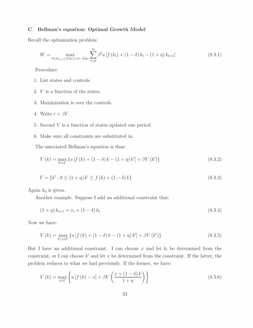
C Bellman’s equation: Optimal Growth Model

Recall the optimization problem:

W = max0≤kt+1≤f(kt)+(1−δ)kt

∞∑

t=0

βtu [f (kt) + (1− δ) kt − (1 + η) kt+1] (8.3.1)

Procedure:

1. List states and controls.

2. V is a function of the states.

3. Maximization is over the controls.

4. Write r + βV .

5. Second V is a function of states updated one period.

6. Make sure all constraints are substituted in.

The associated Bellman’s equation is thus:

V (k) = maxk′∈Γ

{u [f (k) + (1− δ) k − (1 + η) k′] + βV (k′)} (8.3.2)

Γ = {k′ : 0 ≤ (1 + η) k′ ≤ f (k) + (1− δ) k} (8.3.3)

Again k0 is given.

Another example. Suppose I add an additional constraint that:

(1 + η) kt+1 = xt + (1− δ) kt (8.3.4)

Now we have:

V (k) = maxk′,x∈Γ

{u [f (k) + (1− δ) k − (1 + η) k′] + βV (k′)} (8.3.5)

But I have an additional constraint. I can choose x and let k′ be determined from the

constraint, or I can choose k′ and let x be determined from the constraint. If the latter, the

problem reduces to what we had previously. If the former, we have:

V (k) = maxx∈Γ

{

u [f (k)− x] + βV

(

x+ (1− δ) k

1 + η

)}

(8.3.6)

33

IX Existence, Uniqueness, and other properties of the value function

A few useful theorems. Again, no need to get into the details, just want to use them.

Theorem (4.6) Lucas and Stokey:

THEOREM 6 Let:

1. r be bounded for all S ∈ Γ and continuous.

2. Γ be non-empty, compact, and continuous.

3. β ∈ (0,1).

Then V exists and is unique.

Surprisingly, bounding r from above is not too difficult. Suppose in the optimal growth

model we assume c = 0 for at t. Then the resource constraint implies capital will evolve

according to:

0 = f (kt) + (1− δ) kt − (1 + η) kt+1 (9.1)

The steady state of this equation is the maximum sustainable capital stock km:

f (km) = (δ + η) km (9.2)

A finite solution exists since f is concave:

So a natural upper bound for r is u (c (km)). However, u is still may be negatively

unbounded at 0 (for example logarithmic utility). But the theorem does extend to the

unbounded case if u does not go too quickly to −∞ as k goes to zero.

Theorem (4.8) Lucas and Stokey:

THEOREM 7 Suppose (1-3) and suppose:

4. r is concave.

5. Γ is convex.

Then V is concave and the optimal policy function S ′ = h (S) is continuous and single valued.

Theorem (4.11) Lucas and Stokey (Benveniste and Scheinkman, 1979).

THEOREM 8 Envelope theorem. Suppose (1-5) and:

34

km

(η+δ)k

f (k)

f

k

Figure 15: Maximum Capital Stock.

6. r is C1.

7. h (S0) is on the interior of S. (ie the solution is interior).

Then V is differentiable at S0, with derivative:

vs (S0) = rs (S0, h (S0)) (9.3)

Mathematically:

vs (S0) = rs (S0, h (S0)) + hs (S0) (r2 (S0, h (S0)) + βVs (h (S0))) (9.4)

Here the second term is zero due to the first order condition.

Theorem (4.11) is especially useful. It shows that we can apply the envelope theorem to

the Bellman’s equation. We are going to use this a bunch, it will let us solve easily for the

steady state and establish how the value function changes with the states.

Based on papers by Benveniste and Scheinkman (1979) and Araujo and Scheinkman

(1981) it was previously thought that exceptionally strong conditions were required for twice

differentiability of the value function. Twice differentiability is important because it implies

differentiability of the policy function. So Lucas and Stokey and Sargent go through a lot

of hoops trying to avid differentiating h. However, recent results by Santos have shown that

35

twice differentiability. can be had with relatively mild restrictions.

Santos (1991), theorem (2.1) (see also Santos, 1994 and Araujo, 1989).

THEOREM 9 Suppose (1-7) and let:

8. r is twice differentiable at S0.

9. The Hessian of r is negative definite.

10. The eigenvalues of the Hessian of r are bounded and non-zero.

Then V is C2 at S0, and h is C1 at S0.

So the value function is well-behaved, we can work with it analytically. Because the

Bellman’s equation is recursive, we can also use it to solve for V and h numerically.

X Using the Bellman’s equation: first order conditions and comparative statics

of growth model

A First order condition

We have:

V (k) = maxk′∈Γ

{u [f (k) + (1− δ) k − (1 + η) k′] + βV (k′)} (10.1)

The first order necessary condition is thus:

− (1 + η) uc [f (k) + (1− δ) k − (1 + η) k′] + βVk (k′) = 0 (10.2)

So the marginal utility of consumption is the first term, the marginal utility of investment

is the second term. Why? Note that V represents the future of marginal value of all the

capital (k′) we invest in. Hence the total value of investment is V (k′). Note that k′ = h (k)

is defined implicitly from the first order condition. Hence know V if and only if we know h.

Decision rule is of course time invariant.

Why no transversality condition? In fact, we have assumed that u is bounded, and hence

V is bounded. Thus we have in fact already ruled out Ponzi schemes. Thus the transversality

condition is satisfied, implicitly.

36

B Comparative Statics

1 Graphically

In the old days, people worked a lot with graphs because of lack of differentiability. Still

instructive though.

c(k′) = 0 c(k′2) = 0k′2

(1+η)Uc (k2)

(1+η)Uc (k)

k′

Uc

k′

βVK (k′)

Figure 16: First Order Condition, Growth Model.

Note the graph of the MU of consumption follows from uc > 0, ucc < 0, and Inada

conditions. Graph of MU investment follows from concavity of V . Hence graph implies that

for k2 > k we have k′∗2 > k′∗. Hence hk > 0.

2 Via the implicit function theorem

Substituting the solution into the first order condition yields an identity:

− (1 + η) uc [f (k) + (1− δ) k − (1 + η)h (k)] + βVk (h (k)) ≡ 0 (10.3)

Hence we can take the derivative of both sides with respect to k.

− (1 + η) ucc

[

fk + (1− δ)− (1 + η) hk

]

+ βVkkhk = 0 (10.4)

37

Solving for hk gives:

hk =

ucc

[

fk + (1− δ)

]

(1 + η)2 ucc + βVkk

(10.5)

So we see that hk is positive because u and V are concave.

XI Envelope condition

From Theorem (8), we can use the envelope theorem on the Bellman’s equation:

VS (S) = rs (S, S′∗) (11.1)

The envelope equation is used for several purposes.

1. We can use the envelope equation to solve for the steady state.

2. We can use the envelope equation to find the impact of the state variables on the total

welfare.

3. We can recover the Euler equations.

4. We can use the envelope equation to examine the transition path.

5. We can use the envelope equation to solve for the value function and policy function

in special cases.

For the optimal growth model we have:

1. Impact of k on welfare:

Vk (k) = uc

[

f (k) + (1− δ) k − (1 + η) k′

] [

fk (k) + 1− δ

]

(11.2)

Because the marginal utility of consumption is positive and the marginal product of

capital is positive, we see that the marginal value of capital is positive. The above

equation shows that the marginal value of capital is equal to the marginal utility that

the return on capital brings.

38

2. Solve for the steady state. The envelope equation, evaluated at the steady state is:

Vk

(

k)

= uc (c)

[

fk(

k)

+ 1− δ

]

(11.3)

Recall that the first order condition at the steady state is:

(1 + η)uc (c) = βVk

(

k)

(11.4)

Putting these two together gives:

1 + η = β

[

fk(

k)

+ 1− δ

]

(11.5)

This is just the equation examined earlier for the modified golden rule.

3. Recover the Euler equations:

Vk (kt) = uc (ct)

[

fk (kt) + 1− δ

]

(11.6)

(1 + η)uc (ct) = βVk (kt+1) (11.7)

Hence,

βuc (ct+1)

[

fk (kt+1) + 1− δ

]

= (1 + η)uc (ct) (11.8)

But what happened to the transversality condition? Well, conditions imposed on V

imply transversality condition holds. Hence there is some loss of information when we

substitute out for Vk.

39

XII Transitional Dynamics of Growth Model

A Convergence to Steady State

We have examined the steady state properties, getting important insights such as the mod-

ified golden rule. Now let’s look at the transitional dynamics. The dynamics of the growth

model are determined from the optimal policy function:

k′ = h (k) , k0 given (12.1)

Here h is the implicit function defined via the first order conditions. We know:

• h is continuous and increasing in k.

• There exists a steady state k > 0 which satisfies:

1 + η = β

[

fk(

k)

+ 1− δ

]

(12.2)

• The resource constraint,

(1 + η) k′ ≤ f (k) + (1− δ) k, (12.3)

implies that:

limk→0

h (k) = 0. (12.4)

Hence there are two possibilities:

40

h(k)K’

K

K’=K

h(k)

K’

K

K’=K

Figure 17: Possible Convergence Paths, Growth Model.

Hence if the policy function is convex, we have an unstable steady state and the capital

level explodes or falls to zero. If the policy function is concave, we have a stable steady state

(stable balanced growth path). To find out we can use a little proof:

The FOC and envelope are:

(1 + η)uc [f (k) + (1− δ) k − (1 + η) k′] = βVk (k′) (12.5)

Vk (k) = uc

[

f (k) + (1− δ) k − (1 + η) k′

] [

fk (k) + 1− δ

]

(12.6)

Next note that since V is concave, Vk is decreasing in k. Hence:

[

Vk (k)− Vk (k′)

]

(k − k′) ≤ 0 (12.7)

Hence:

uc (·)

[

fk (k) + 1− δ −1 + η

β

]

(k − k′) ≤ 0 (12.8)

Let us do the population utility, the per capita case is analogous. Then:

[

(fk (k) + 1− δ)− (1 + ρ)

]

(k − k′) ≤ 0 (12.9)

[

fk (k)− δ − ρ

]

(k − k′) ≤ 0 (12.10)

41

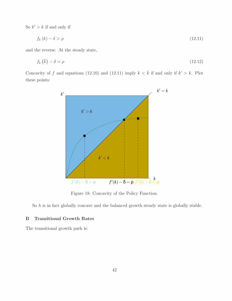
So k′ > k if and only if

fk (k)− δ > ρ (12.11)

and the reverse. At the steady state,

fk(

k)

− δ = ρ (12.12)

Concavity of f and equations (12.10) and (12.11) imply k < k if and only if k′ > k. Plot

these points:

f ′(k)−δ = ρ

k′ = k

k′ > k

k

k′ < k

f ′(k)−δ < ρf ′(k)−δ > ρ

k′

Figure 18: Concavity of the Policy Function.

So h is in fact globally concave and the balanced growth steady state is globally stable.

B Transitional Growth Rates

The transitional growth path is:

42

tk1−k0

k0

k2−k1k1

k3−k2k2

k′−kk

k′ k′ = k

h(k)

k

Figure 19: Transitional Dynamics.

How do I know the growth rate declines? This follow from the concavity of h. The

growth rate in k is:

g (k) =k′ − k

k=

h (k)

k− 1 (12.13)

43

We wish to show that

gk (k) =khk (k)− h (k)

k2< 0 (12.14)

Or:

hk (k) k < h (k) (12.15)

Since h is concave, we know from property 4 of concave functions and equation (12.4), that

the above equation is satisfied (choose d equal to 0 and k). Thus g is decreasing.

So the growth rate of capital is highest at low capital levels, in fact it is higher than the

population growth rate η. Eventually the growth rate of capital slows to rate η. Further,

the speed of the convergence to balanced growth is determined by the concavity of h. If h is

very concave, convergence is quick, especially early on.

C Catch-Up

Note an implication of declining growth rates:

Definition 11 CONDITIONAL CONVERGENCE HYPOTHESIS: Assuming identical pref-

erences and technology, countries should converge to identical growth rates of per capita GDP

or total GDP and/or identical levels of per capita GDP or total GDP.

Definition 12 ABSOLUTE CONVERGENCE HYPOTHESIS: countries converge to growth

rates and/or levels which are identical irrespective of preferences or technology.

We have several definitions of convergence. In the model done in class, for example, the

steady state has zero growth in per capita GDP. The model predicts absolute convergence

of the growth rate of per capita GDP (to zero). Conversely, the level of GDP converges

to f(

k)

, where k satisfies f(

k)

− δ = ρ (for the population utility case). Therefore, we

have conditional, but not absolute, convergence of the levels of per capita GDP. Countries

with identical technologies will converge to the same f(

k)

, but countries with a different

technology will converge to a different k, and a different level of per capita GDP.

Conditional convergence has mixed evidence. Barro’s experiment: compare “similar”

countries. After a shock hits one country but not another, compare growth rates. For

example, Japan after WWII and US, Australia, and Canada. None of the last three suffered

much damage, but Japan was devastated. Japan then grew faster. See graph. Similar results

hold across the developed world. Results also hold for US states after Civil War, although

44

there is some sensitivity to what initial year is used. Results don’t much hold in Africa and

other less developed countries which have not grown at a faster rate.

Convergence hypothesis in general does not hold. See Romer’s graph.

There seems to be a J-curve convergence, middle countries grow faster than either poor

or rich countries. There is even some evidence for conditional convergence, with differences

based on such things as lack of access to credit and stock markets, corruption, cycles of

poverty, and differences in education and life expectancy.

Further, growth per capita does not go to zero, as predicted. We can exogenously cause

per capita growth to be greater than zero by adding in the technical change parameter as in

the homework.

XIII Analytic Solutions to Growth Models

The recursive formulation of the Bellman’s equation gives us the ability to solve growth

models. This is pretty rare, even when everything is rigged. Still, it sometimes happens and

doing so builds some intuition.

A value function iteration

General procedure: Start with an initial value function and iterate forward. Suppose we

have the following specification. Let δ = 1, η = 0 and:

f (k) = Akγ (13.1.1)

u = log (c) (13.1.2)

Then:

Vi (k) = maxk′∈Γ

{log [Akγ − k′] + βVi−1 (k′)} (13.1.3)

Start with an initial value, say V0 = 0. What is the economic interpretation of V0 = 0?

What is the optimal investment? Clearly k′ = 0. Then we have:

V1 (k) = log [Akγ ] = γ log (k) + log (A) (13.1.4)

45

Thus:

V2 (k) = maxk′∈Γ

{log [Akγ − k′] + β (γ log (k′) + log (A))} (13.1.5)

The FOC for this problem is:

1

Akγ − k′=

βγ

k′(13.1.6)

Hence:

k′ =βγ

1 + βγAkγ (13.1.7)

So the optimal policy is to invest a constant fraction of income. One can then show that the

value function reduces to:

V2 (k) = E2 + F2 log (k) (13.1.8)

Here E and F are constants. For example Fi takes the form

Fi = γ(

1 + βγ + . . .+ (βγ)i)

(13.1.9)

Notice that the functional form of the value function did not change, only the constants

changed (unlike in step one). Taking limits as i → ∞, we get the solution that F = 11−βγ

and the policy function is:

k′ = βγAkγ (13.1.10)

B Guess and Verify

We might guess a solution of the form:

E + F log (k) (13.2.1)

Where did the guess come from? Well, see above. Procedure:

1. Solve the FOC for the optimal policy.

2. Compute the envelope equation, substitute in the optimal policy, and solve for the

undetermined coefficients (F ).

3. Plug everything back into the value function equation and solve for E.

46

EXERCISE: I invite you to try this on your own as an exercise.

XIV Quantitative Analysis of the Growth Model

King and Rebelo (1993) examined the predictions of the growth model from a quantitative

perspective. That is KR used likely parameter values and solved the growth model. The

parameterization is as in the homework with Cobb-Douglass production and CRR utility:

f (k) = Akγ (14.0.1)

U (c) =c1−σ − 1

1− σ(14.0.2)

Several studies on micro-level data estimate σ at near one, which is logarithmic utility. γ

is estimated to be around .3. KR solved the growth model, plugged in these numbers and

then examined cases such as Japan after WWII. (put graph up).

The results are not encouraging for the growth model. The growth model predicts ex-

tremely fast growth for poor countries. Should not require 30 years but instead about 5 to

return to balanced growth. Initial interest rates are near 500% to attract investment. But

this is not so in Japan (or elsewhere). Note the interest rate is r = fk (k)− δ. So the interest

rate should fall as we approach the steady state.

Can we parameterize the model in such a way as to slow down growth? Yes. Recall that1σmeasures the Intertemporal rate of substitution across time. If 1/σ is very small, we prefer

very smooth consumption. Thus even high interest rates do not persuade us to invest a lot

early and consume a lot later. We prefer to consume an even amount. KR estimates we

need σ = 10. Of course, this implies unrealistically high risk aversion. Note, this problem

might be solved if a utility function had separate parameters for risk and for substitution

over time.

XV Summary of Results of Growth Model

1. Small economies have higher per-capita growth rates. The marginal product of capital

is higher, therefore, invest more.

2. Rate of growth on transition path is determined by the concavity of optimal investment

function, which is in turn determined by concavity of u and f .

47

3. Always converge to balanced growth.

4. At balanced growth, K, I, Y , C, and L all grow at the same rate, the rate of growth

in labor.

5. At balanced growth we have constant ratios: K/Y is constant, I/Y is constant, etc.

6. CATCH UP. Poor countries grow faster than rich countries, growth rates converge.

7. Per capita growth rate is zero, but is positive and constant if the model has exogenous

technological change.

8. Convergence is very quick (5-20 years), for reasonable parameter values.

48

COMPETITIVE GROWTH MODEL

I Assumptions

We are going to now solve the competitive version of the optimal growth model. Although

the allocations are the same as in the social planning problem, it will be useful to compare

the two models. After this point, most models will have externalities or other market failures,

which means we will have to solve the competitive model directly. Further, by finding prices

we can gain further insights not possible from the social planning problem, which only gives

allocations.

A Retain Assumptions

All models from this point out will be variants of the optimal growth model. Therefore, we

will retain all the assumptions of the optimal growth model, except for the changes noted

below.

B Firms

1 Capital ownership

We will assume households own capital and labor and rent them to firms. Firms renting

capital is certainly consistent with both public corporations and sole proprietorships. The

share of stock establishes ownership of the firm’s capital. That the stockholder’s capital is

stored at the firm is a matter of convenience. Further, the stockholder is also entitled to the

corporation’s profits, which are in fact the capital rental payments. For sole proprietorships,

the owner certainly owns the capital and is also entitled to the profits.

2 Number of Firms

Assume there exists one firm per household. With CRS, the number of firms is indeterminite.

Definition 13 A variable x is indeterminate if any value of x is consistent with the model.

Indeterminacy of the number of firms is proved in section F.

3 What are Firms?

Firms are endowed with a production technology F . Other than that, firms are simply the

way workers and capital owners are organized.

49

C Prices

1 Consumption Goods

Let the price of the consumption good, Pt be normalized to one. Consumption goods

(shmoos) are thus the numeraire good. We quote all other prices in terms of the numeraire

good (ie. my wage is w shmoos per hour). Typically, money is the numeraire, but we have

no money in this model.

2 Rental rates

The rental rate of labor is the wage: wt units of consumption goods per unit of labor L. The

rental rate of capital is rt units of consumption goods per unit of capital rented.

D Competitive Economy

The model that of a competitive economy: firms and households take prices as given. Prices,

in turn, equate supply and demand.

II Firm Problem

A Profit maximization

Firms maximize profits. It is straightforward to show that owners of the firm prefer the

firm to maximize profits. In a version of the model where firms own the capital and make

investment decisions, profit maximization is equivalent to maximizing the present discounted

value of a share.

B Firm Problem

Let profits be Π.

Π = maxKd

t ,Ldt

{

1 · F(

Kdt , L

dt

)

− rtKdt − wtL

dt

}

(2.2.1)

Here superscript d indicates firm demand.

50

C First order conditions

The problem of the firm is static: all of the dynamic savings are done by the households.

The first order conditions are thus:

rt = Fk

(

Kdt , L

dt

)

(2.3.2)

wt = Fl

(

Kdt , L

dt

)

(2.3.3)

These equations determine kd and ld as a function of the prices. They are demand curves.

From the firm’s point of view, it is only worth hiring an additional unit of a factor if the

output that unit produces exceeds the cost. If hiring one worker results in the production

of 10 more shmoos and the worker costs 8 shmoos per hour then hire: profits will rise by 2

shmoos.

As with the optimal growth model, we use the properties of CRS to simplify. Note that:

F (K,L) = L · F

(

K

L,1

)

(2.3.4)

Hence:

Fk (K,L) = L · Fk

(

K

L,1

)

1

L= Fk

(

K

L,1

)

= fk (k) (2.3.5)

Notice that equation (2.3.5 shows that if the production function is constant returns to scale,

the marginal products are homogeneous degree 0. The general version of this theorem is:

THEOREM 10 Let F (X) be homogeneous degree α in X = [x1 . . . xn]. Then Fi (X) is

homogeneous degree α− 1.

For the other marginal product, we have:

FL (K,L) = F

(

K

L,1

)

− LFk

(

K

L,1

)

K

L2= f (k)− kfk (k) = FL (k,1) (2.3.6)

Notice that we have also proved here that if F is homogeneous degree 1, then marginal

product of labor is homogeneous degree 0.

Let kd = Kd/Ld, then:

rt = fk(

kdt

)

(2.3.7)

51

wt = f(

kdt

)

− kdt fk(

kdt

)

(2.3.8)

D Zero Profits

We have:

Πt = Ldt f(

kdt

)

− fk(

kdt

)

Kdt −

(

f(

kdt

)

− kdt fk(

kdt

))

Ldt (2.4.9)

= −fk(

kdt

)

kdtL

dt + fk

(

kdt

)

kdtL

dt = 0 (2.4.10)

So profits are equal to zero. Question: are accounting profits or economic profits equal to

zero? What are accounting profits in the model?

E Equilibrium

In equilibrium, supply equals demand: kdt = ks

t . Furthermore, suppose that Lt firms exist.

Then since all firms are identical, they choose identical amounts of the aggregate capital

stock Kt and labor stock Lt. Hence equilibrium labor per firm is Lt/Lt = 1. Equilibrium

total capital per firm is similarly Kt/Lt = kt. Note here I am anticipating that households

will supply all labor and capital they possess. There is no reason to leave a working factory

idle. Therefore, Kd = Ks = K and the same for L. Therefore in equilibrium:

kdt =

Kdt

Ldt

=Kt

Lt

= kt. (2.5.11)

Hence in equilibrium:

rt = fk (kt) (2.5.12)

wt = f (kt)− ktfk (kt) (2.5.13)

These equations determine the prices r and w given the state k. They are equilibrium

conditions. Equilibrium conditions determine prices.

F Indeterminacy

From the profit condition (2.2.1) we have:

Π (λK, λL) = F (λKt, λLt)− rtλKt − wtλLt (2.6.14)

52

= λαF (Kt, Lt)− rtλKt − wtλLt (2.6.15)

= λ(

λα−1F (Kt, Lt)− rtKt − wtLt

)

(2.6.16)

Now suppose α = 1. Then Π (λK, λL) = λΠ (K,L). Consider then any merger which

would increase the size of the firm by λ > 1 or any spinoff which reduces the size of the firm

by λ < 1. Profits are unchanged: the profits of the combined firm equals the sum of the

profits of the firms apart. Therefore CRS implies the number of firms is indeterminate. In

contrast, if α > 1, then firms increase profits by merging or if α < 1 by spinning off into

smaller firms. Therefore, CRS can be viewed as an equilibrium condition where firms have

no incentive to change size.

III Household Problem

A Normalized Problem

Households maximize:

U = max

∞∑

t=0

βtu (Ct) (3.1.1)

The maximization is subject to the budget constraint. The budget constraint sets income

equal to expenses. Consider a particular household, labeled h.

rtKht + wtL

ht + (1− δ)Kh

t = Ct +Kht+1 (3.1.2)

Normalize:

rtkht + wt + (1− δ) kh

t = cht + kht+1 (1 + η) (3.1.3)

Notice that the household will supply all it’s capital. There is no sense in not renting a

factory. Similarly, the household has no preference for leisure and hence will rent out all it’s

labor. Hence Lht = 1 (one can think of this as working 100% of available time) and cht = Ct.

RULE: for maximization you can maximize the control variables in any order, and substitute

in the solution if you want.

53

B Recursive Problem

1 Problem

We have a new kind of variable: prices. Prices are taken as given, kind of like a state, but

also determined, like a control (but determined by equilibrium conditions, not first order

conditions). Since we have no easy way to deal with these, let us try substituting out.

RULE: you can always substitute one variable determined in equilibrium for another. Let’s

substitute out using the firm first order conditions in equilibrum.

fk (kt) kht + f (kt)− ktfk (kt) + (1− δ) kh

t = ct + kht+1 (1 + η) (3.2.4)

Note that we have reduced the state space by one: if we know the aggregate capital stock

k, then we know the wage and interest rate.

We now divide state variables into two categories, individual states and aggregate states.

Aggregate states are similar to individual states in that they are given today but can change

over time. However, individuals do not consider their effect on aggregate states over time,

since an individual is too small to materially affect the aggregate capital stock per person.

Now we have aggregate state k and individual state kh. Hence:

v(

kh,k)

= maxkh′

{

u

[

f (k) + fk (k)(

kh − k)

+ (1− δ) kh − (1 + η) kh′

]

+ βv(

kh′, k′)

}

(3.2.5)

Checking through the value function, k′ is not a state or control. It is everyone else’s

investment decision, which household h cares about because it will affect future wage and

interest rates. It is determined in equilibrium. We refer to such variables as aggregate

controls. They are determined in equilibrium, but taken as given by the household (the

same as prices).

Overall:

1. Individual states: given today, but the individual may change them over time.

2. Aggregate states: given today, but everyone’s decisions may change them over time.

3. Individual controls: individuals may change these today.

4. Aggregate controls or prices: determined today via equilibrium conditions. Unaf-

fected by an individual.

5. Parameters: constant through time.

54

6. We have v ( individual states, aggregate states ). We max over individual controls. For

each aggregate control/price, we must have an equilibrium condition.

We need an equilibrium condition for each aggregate control or price. Here the individual

decision will be a function kh′ = h (kh, k). Let us suppose an equilibrium in which households

are identical. If households are identical they hold the same amounts of capital kh = k, and

make the same investment decisions kh′ = k′. Thus the equilibrium condition is:

kh = k implies kh′ = k′ = h (k,k) (3.2.6)

2 First order conditions and envelopes

We have:

(1 + η)uc

[

f (k) + fk (k)(

kh − k)

+ (1− δ) kh − (1 + η) kh′

]

= βv1(

kh′, k′)

(3.2.7)

This determines the individual decision kh′. Once again, the marginal utility of consumption

equals the marginal value of investment, divided by the larger population and discounted

back to today.

The envelope equation is:

v1(

kh,k)

= uc

[

f (k) + fk (k)(

kh − k)

+ (1− δ) kh − (1 + η) kh′

]

(fk (k) + 1− δ)(3.2.8)

So again the marginal value of the household’s capital is the gross return net of depreciation

times the value of the return which is the marginal utility of consumption.

Notice from the firm first order condition:

v1(

kh,k)

= uc

[

f (k) + fk (k)(

kh − k)

+ (1− δ) kh − (1 + η) kh′

]

(r + 1− δ) (3.2.9)

So r in the competitive model is a gross interest rate (before depreciation). The household

pays the depreciation, it is not taken out of the firm’s interest payment. This is just account-

ing. If firms handled the depreciation and returned r − δ to the household, the envelope

equation would be identical.

55

IV Equilibrium

Now impose the equilibrium conditions. RULE: impose equilibrium only after finding the

first order conditions and envelope equations.

(1 + η)uc

[

f (k) + (1− δ) k − (1 + η) k′

]

= βv1 (k′, k′) (4.0.1)

v1 (k,k) = uc

[

f (k) + (1− δ) k − (1 + η) k′

]

(fk (k) + 1− δ) (4.0.2)

c = f (k) + (1− δ) k − (1 + η) k′ (4.0.3)

These equations determine the aggregate controls. These completely determine the equilib-

rium allocations of the competitive economy.

It is traditional to define the equilibrium: write down the system of equations and vari-

ables which constitute an equilibrium. The procedure: given all states, an equilibrium is the

set of individual decisions, aggregate decisions, prices and a value function, such that firms

and households optimize, budget constraints are satisfied, resource constraints are satisfied,

and the Bellman equation holds. In the definition, we should see the number of variables

determined equal the number of equations. This is a good check.

Let s =[

kh, k]

denote a vector of individual states and S = [k, k] denote the aggregate

states. Then:

Definition 14 A Recursive Competitive Equilibirum given individual states s =[

kh, k]

and aggregate states s = [k, k], is a set consisting of individual decisions[

kh′ (s) , ch (s)]

,

aggregate decisions [k′ (S) , c (S)], prices [r (S) , w (S)], and a value function v (s) such that

firms optimize (equations 2.5.12 and 2.5.13 hold), households optimize (equation 3.2.7 holds),

the budget constraint is satisfied, the Bellman’s equation holds, and individual decisions are

consistent with aggregate outcomes (equation 3.2.6 holds).

Let us now verify we have a well-defined system of equations. We have 7 unknowns (2

individual decisions, 2 aggregate decisions, 2 prices, and v). We have two firm first order

conditions, 1 household first order condition, 1 budget constraint, and 1 Bellman’s equation.

The equilibrium condition gives us two more equations, one applied to the budget constraint

and another to the household first order condition. So we have 7 equations for 7 unknowns.

56

The budget constraint evaluated at equilibrium yields the resource constraint. Prices

determine who gets what resource. Prices do not add to the total resources available.

V Welfare

A Psuedo Planning problem (PSP)

Recall the equilibrium allocations are:

(1 + η)uc

[

f (k) + (1− δ) k − (1 + η) k′

]

= βv1 (k′, k′) (5.1.1)

v1 (k,k) = uc

[

f (k) + (1− δ) k − (1 + η) k′

]

(fk (k) + 1− δ) (5.1.2)

c = f (k) + (1− δ) k − (1 + η) k′ (5.1.3)

A Psuedo planning problem is a planning problem which generates the same allocations

as the competitive equilibrium. We can construct such a problem as follows:

ν (k) = maxk′

{

u

[

f (k) + (1− δ) k − (1 + η) k′

]

+ βν (k′)

}

(5.1.4)

The first order condition and envelopes are:

(1 + η)uc

[

f (k) + (1− δ) k − (1 + η) k′

]

= βνk (k′) (5.1.5)

νk (k) = uc

[

f (k) + (1− δ) k − (1 + η) k′

]

(fk (k) + 1− δ) (5.1.6)

c = f (k) + (1− δ) k − (1 + η) k′ (5.1.7)

Let c∗ and k′∗ solve the first order condition and resource constraint for the PSP. Let us check

to see if c∗ and k′∗ solves the competitive first order condition and resource constraint. Since

c∗ and k′∗ are identical, we have from (5.1.2) and (5.1.6) that νk (k) = v1 (k, k). But then the

first order condition and resource constraint are the same in the competitive problem as in

the PSP. Therefore, the problems have the same solution and the PSP and the competitive

57

equilibrium have the same allocations.

The main use of the PSP is to come up with a planning problem which is easier to work

with than the competitive model. It often illustrates why a competitive equilibrium is not

welfare maximizing. A second use is for comparative statics. It is generally easier to compute

the derivative hk (k) than h1 (k,k) + h2 (k,k).

B Welfare theorems

Notice that the PSP is the social planning problem. We have thus shown that the Competi-

tive equilibrium with identical households maximizes welfare. There is no role for government

in this problem. Set up a price system and allow households to make individual decisions

that benefit themselves and overall welfare of society is maximized.

In the future we will have externalities or distortions and so in general the Social Planning

problem differs from the PSP. In this case, however, often we can put in a tax or subsidy to

equate the allocations.

58

Endogenous Growth Models

I Regularities

Recall that we said that the optimal growth model did not do very well in four respects:

• Convergence doesn’t always occur, some poor countries grow slowly or not at all.

• Predicted time to convergence is too fast.

• We still don’t know why per-capita income rises. We know only that total factor

productivity rises. Why does total factor productivity rise?

• Productivity increases are constant and are free. But in fact as we will see things

become more difficult to invent over time.

In Endogenous growth models, the growth rate of output per capita is endogenous. The

hope is that by explaining what determines the growth rate, we can determine why some

countries do not grow or grow slowly.

Endogenous Growth papers:

• JEP Winter 1994.

• Romer JPE, 1986, 1990.

• Lucas, 1988 JME.

• Jones and Manuelli, JPE 1990.

• Segerstrom 1998.

II AK MODEL

A Background

Recall that there are two ways to slow convergence in the optimal growth model, increase

σ (increase desire for smooth consumption) or increase γ. Returns to capital increase more

slowly as a country becomes poor,

r = fk (k)− δ =γA

k1−γ− δ, (2.1.1)

59

is more constant in k.

But remember γ ≈ .33. So we have to justify a higher γ. There are three justifications

(which indicates none are very convincing ...).

1 Local technology

Suppose A, technology is determined at the local level, and there is an externality in that

knowledge spills over to other firms without cost. Ie other firms may use the technology

without paying. Then firm j’s production function is:

Yj = A (K,L)Kγj L

1−γj (2.1.2)

Note: the externality breaks the link between the social planning problem and competitive

equilibrium. Further, we can continue to assume that γ = .33, since firms don’t get paid

when other firms steal their technology. Suppose:

A (K,L) = AKζL−ζ (2.1.3)

Then:

Yj = AKζL−ζKγj L

1−γj (2.1.4)

Yj

Lj

= A

(

K

L

)ζ (Kj

Lj

)γ

(2.1.5)

If all firms are identical, Kj =KL, Lj =

LL= 1, Yj =

YLand:

y = Akγ+ζ (2.1.6)

For the special case of γ + ζ = 1, we have the AK model. Estimates are only as high

as .75, however. (Romer JEP). Further, small deviations away from one possibly have big

long term implications, if γ + ζ is even slightly less than one, the model is the same as the

optimal growth again.

2 Average product of capital

Assume 1− δ = η = 0. Then:

c = f (k)− k′ (2.1.7)

60

Assume further that average product of capital is constant, as it is along balanced growth:

f (k)

k=

y

k= A (2.1.8)

Then:

c =f (k)

kk − k′ (2.1.9)

c = Ak − k′ (2.1.10)

Of course the above assumes we are in a balanced growth path. But one of the main things

we are concerned about is the speed of transition to the steady state. This question cannot

be answered if we rely on the average product of capital argument.

3 total capital

Do not distinguish between capital and labor, instead have a single capital k which includes

human capital. Retain the HD 1 assumption. Then f (k) = Ak.

However, by switching to total capital, we ignore many differences between physical and

human capital. The depreciation rates are likely to be quite different, for example. The

desire to have kids and increase the human capital stock probably has a lot more to do with

their value as consumption than on the return kids will generate. Perhaps one might find

these assumptions unconvincing, but the AK model is simple and provides good intuition.

B Assumptions

Retain all assumptions of the optimal growth model, except let f (k) = Ak. The value

function is then:

v (k) = maxk′

{

u(

Ak + (1− δ) k − (1 + η) k′)

+ βv (k′)}

(2.2.1)

Let A ≡ A+ 1− δ, then:

v (k) = maxk′

{u (Ak − (1 + η) k′) + βv (k′)} (2.2.2)

61

C FOC’s, envelope equation, and Steady state

The first order condition and envelope equation are:

(1 + η)uc (c) = βvk (k′) (2.3.1)

vk (k) = Auc (.) (2.3.2)

Using population utility, the steady state is thus:

1 + η = βA (2.3.3)

For either population or per capita:

1 + ρ = A = A+ 1− δ (2.3.4)

ρ = A− δ. (2.3.5)

Hence a steady state exists only for this special case. In this case, any k satisfies the above

equation and is thus a steady state.

D Transitional dynamics and endogenous growth

To get the transitional dynamics, we first show that investment spending is increasing in the

capital stock:

− (1 + η) uc (c) + βvk (k′) = 0 (2.4.1)

(1 + η)ucchk + βvkkhk − uccA = 0 (2.4.2)

hk =uccA

(1 + η)ucc + βvkk> 0 (2.4.3)

We still know that h (0) = 0. Finally, v is concave, we know:

[

vk (k)− vk (k′)

]

(k − k′) ≤ 0 (2.4.4)

62

[

βA− (1 + η)

]

(k − k′) ≤ 0 (2.4.5)

Using the population utility:

[

A+ 1− δ − (1 + ρ)

]

(k − k′) ≤ 0, (2.4.6)

[

A− δ − ρ

]

(k − k′) ≤ 0, (2.4.7)

Hence if A− δ > ρ (or alternatively βA > 1) then k < k′ and vice versa.

Graphically:

β

A=1β

A<1β

A>1

k’<k

k’

k

k’>k

k’=k

Figure 20: Transitional Dynamics of the AK model.

Hence for A− δ > ρ we have capital growing without bound. If not, capital goes to zero.

Definition 15 Endogenous growth occurs if capital diverges to infinity.

So in the AK model, endogenous growth occurs if and only if A− δ > ρ.

The AK model says that endogenous growth occurs if the interest rate is above the rate

63

of time preference for all k. In this case, no matter how rich we are, the interest rate will

continue to attract enough savings to keep the growth going.

We also would like the above condition for endogenous growth to be independent of η,

so that exogenous growth in population does by itself generate endogenous growth. Here

A− δ > ρ is independent of η, as desired.

Finally, since f (k) is no longer concave, no maximum sustainable capital stock exists

here.

c = 0 = Ak − (1 + η) k, (2.4.8)

If the condition for endogenous growth is satisfied, the right hand side is positive and no

maximum sustainable capital stock exists.

E Growth Rate

It is easy to see from figure 20 that k′ = h (k) cannot be concave or else a steady state would

exist. Thus, in the endogenous growth case h (k) is at least weakly convex. Therefore:

g =h (k)− k

k=

h (k)

k− 1, (2.5.1)

gk (k) =hk (k) k − h (k)

k2, (2.5.2)

gk (k) ≥ 0 ⇔ hk (k) k ≥ h (k) . (2.5.3)

The above equation holds since h is weakly convex. Therefore, the growth rate increases with

k and rich countries grow as fast or faster than poor countries. No conditional convergence

exists.

64

kt

t

log(k), rich

log(k), poork0, poor

k0, rich

Figure 21: Transition of two countries, one poor and the other wealthy.

So the AK model simply eliminates two assumptions (Inada conditions and diminishing

marginal product of capital), both by letting γ = 1. The result of this small change is that

the model addresses several regularities of section I:

1. Convergence doesn’t ever occur, because the interest rate is the same in poor and rich

countries.

2. Convergence is much slower, in the sense that there is no convergence.

3. Per capita incomes continue to rise because the interest rate remains above the rate of

time preference (because the marginal product of capital does not diminish).

Like the game whack-a-mole, however, solving the above 3 problems has created new

ones.

1. Most estimates of γ are not near one.

2. Convergence sometimes does occur (e.g. Japan, Europe after WWII), which the AK

model does not predict.

3. Convergence is now too slow.

4. Productivity growth is still free (firms steal other firm’s technology).

5. Scale effect: see section H.

65

F Competitive Model With Spillovers

The social planning problem above does not give the same allocations as the competitive

equilibrium. Let us derive the competitive allocations.

1 Firm and household problems

Suppose we return to the idea that spillovers exist. The production function is:

Yt = AKζt k

γt l

1−γt . (2.6.1)

Here K is the aggregate per capital capital stock per person and k is the capital stock of a

firm. Now ζ = 1− γ so,

Yt = A (K,L) kγt l

1−γt = AK1−γ

t kγt l

1−γt . (2.6.2)

The firm maximizes profits:

π = maxkt

{

AK1−γt kγ

t l1−γt − rtkt − wtlt.

}

(2.6.3)

The first order conditions are:

rt = γAK1−γt kγ−1

t l1−γt , (2.6.4)

wt = (1− γ)AK1−γt kγ

t l−γt . (2.6.5)

In equilibrium kt = Kt and lt = 1 with Lt firms so:

rt = γA, (2.6.6)

wt = (1− γ)AK. (2.6.7)

Notice the problem: the firm is not paid for the increase in productivity it’s research generates

in other firms. So the market does not provide enough incentives to rent capital. The interest

rate γA is less than the return to capital, A.

The household problem is unchanged from the competitive optimal growth, except that

the interest rate is different. Let k denote individual capital, and K the economy wide

66

average per capita capital stock, then:

v (k,K) = maxkh′

{

u

[

(1− γ)AK + (γA+ 1− δ) k − (1 + η) k′

]

+ βv (k′, K ′)

}

(2.6.8)

2 First order conditions

The first order condition at equilibrium is:

(1 + η)uc [C] = βvk (K′, K ′) . (2.6.9)

The envelope condition at equilibrium is:

vk (K,K) = uc [C] (γA+ 1− δ) . (2.6.10)

C = (A + 1− δ)K − (1 + η)K ′. (2.6.11)

The first order condition is unchanged, but the smaller envelope means there is less incentive

to invest.

3 Endogenous Growth

EXERCISE: compute the condition for endogenous growth for the competitive model.

4 PSP

Looking at (2.6.9)-(2.6.11), we see that the competitive equilibrium does not have the same

allocations as the social planning problem, due to the different envelope condition. Does a

PSP exist? For the special case of δ = 1, we can change the incentive to save by altering

the discount factor. Let βx be the new discount factor (and hence we are solve a Pseudo

problem since the discount factor is in reality equal to β). Then:

ν (K) = maxK ′

{

u

[

(A+ 1− δ)K − (1 + η) k′

]

+ xβν (K ′)

}

. (2.6.12)

The first order condition and envelope are:

(1 + η)uc [C] = βxνk (K′) . (2.6.13)

νk (K) = uc [C]A. (2.6.14)

67

C = AK − (1 + η)K ′. (2.6.15)

So for δ = 1, we match the envelope if:

νk (K) =vk (K,K)

γ. (2.6.16)

The first order condition matches if:

vk (K′, K ′) = xνk (K

′) . (2.6.17)

Combining the last two equations, we see that we need:

x = γ. (2.6.18)

The competitive problem is equivalent to a planning problem with less concern about the

future.

G Interest subsidy

Suppose the government offers an interest subsidy, τ , per unit of capital rented, paid to the

household. The government uses a lump sum tax −TR to finance this expenditure. The

government budget constraint is then:

−TR = τrK = τγAK. (2.7.19)

Adding this to the household problem gives:

v (k,K) = maxkh′

{

u

[

(1− γ)AK + (γA + 1− δ) k − (1 + η) k′ − TR + τrk

]

+βv (k′, K ′)

}

(2.7.20)

So now the household has an extra incentive to save in that rented capital receives a subsidy.

We need to account for TR, which is an aggregate state. But we can use the government

constraint to recognize that TR is a function of the aggregate state K and thus we do not

68

need to keep separate track of it:

v (k,K) = maxkh′

{

u

[

(1− γ)AK + (γA + 1− δ) k − (1 + η) k′+

τγA (k −K)

]

+ βv (k′, K ′)

}

(2.7.21)

The first order condition and envelope at equilibrium are:

(1 + η)uc [C] = βvk (K′, K ′) . (2.7.22)

The envelope condition at equilibrium is:

vk (K,K) = uc [C] ((1 + τ) γA+ 1− δ) . (2.7.23)

C = AK − (1 + η)K ′. (2.7.24)

Can the competitive equilibrium with an interest subsidy maximize welfare? We need

to make sure the allocations are the same as the social planning problem. The first order

condition and consumption equation are the same. To equate the envelope, we set:

(1 + τ) γA = A, (2.7.25)

τ =1− γ

γ. (2.7.26)

The optimal interest subsidy equals the marginal social product of knowledge:

subsidy = τr =1− γ

γγA = (1− γ)A. (2.7.27)

With an interest subsidy equal to the marginal social value of knowledge, the competi-

tive problem and social planning problems give identical allocations. Thus the competitive

economy with subsidies maximizes welfore. This illustrates the general point that when the

competitive economy fails to maximize welfare, the solution is generally just to change the

incentives so that private actors are motivated to act in a way which maximizes the social

good.

69

H Scale effect

The most difficult problem with the AK model is what is known as the “scale effect.”

Definition 16 Scale Effect: Countries with larger absolute population sizes grow faster per

capita than smaller countries.

The scale effect is clearly not present in the data. Small developed countries like Luxemborg

or Norway grow as fast or faster than many large countries like Brazil or India. In the optimal

growth model, the growth rate of per capita output does not depend on the population growth

rate.

To see the scale effect, suppose a more intuitive assumption that more labor does not

decrease overall knowledge. That is, suppose:

At = AKζt . (2.8.1)

Here I have assumed labor has no effect on knowledge. Any positive effect of labor on

knowledge will only make the problem worse. Now if ζ = 1− γ,

Yj = AK1−γKγj L

1−γj (2.8.2)

In equilibrium with L firms, Yj =YLand the same for Kj and Lj = 1:

y =Y

L= AK1−γ

(

K

L

)γ

=K

Lγ=

K

LL1−γ . (2.8.3)

Thus we should see countries with larger populations have larger output per capita. Further,

we have:

r = γAK1−γKγ−1j L1−γ

j = γAK1−γ

(

K

L

)γ−1

= γAL1−γ . (2.8.4)

So the interest rate is also an increasing function of population. Larger countries should

have higher interest rates and faster per capita growth. This is also not supported by the

data (Jones, 1995).

Sometimes we can fix the scale effect by assuming small countries observe world capital

and labor to increase TFP:

At = AKζw,tL

1−ζw,t . (2.8.5)

70

Now suppose for example there exists n countries of equal size. Then we have Kw = Kn

and Lw = Ln:

At = AnKζL1−ζ . (2.8.6)

So:

Y

L= AnL

(

K

L

)ζ+γ

= AnLk. (2.8.7)

Clearly this does not fix the problem for the AK model with spillovers.

I Conclusions

The AK model implies no conditional convergence, which is a little strong. Recall the optimal

growth model’s prediction of conditional convergence worked well in many examples, such as

after WWII and in the US after the civil war. The AK model also has a scale effect, which

does not match the data.

Note that we are also studying the social planning problem even though the competitive

equilibrium and social planning problem do not give the same allocations. It is possible for

the competitive equilibrium absent subsidies to converge to zero growth while the competitive

equilibirum with subsdies to have endogenous growth. In this case, the answer to why some

countries do not grow would be lack of capital subsidies.

Two more natural places to look:

• Look at the process generating productivity advances, and government policy in this

area. How do problems in developed economics such as wars, looting, theft, and

corruption affect the process which generates productivity advances?

• Look at the process of human and physical capital accumulation and how these are

affected by the same problems.

Nonetheless, we have learned that the assumption of diminishing marginal product drives

many of the results of the optimal growth model.

71

III Quality Ladder Model

A Concepts

This model is based on Segerstrom (1998). This model looks more closely at the process by

which productivity advances occur.

1 TFP advances as improvements in quality

Here we suppose that TFP advances come in the form of improvements to the quality of

products. An innovation allows a higher quality product to be produced at the same price.

Therefore, utility increases, but the cost of production stays the same. An example is

the move from cassette walkmans to CD walkmans to Ipods. Adjusted for inflation, these

products have similar production costs but each change represents a higher level of quality.

2 Monopolistic inventors

Inventors are typically granted monopoly rights through the patent system, and are not paid

a subsidy equal to the marginal social product of knowledge. So the monopoly “subsidy”

may actually be worth more or less than the marginal social product of knowledge. We may

therefore need a tax or subsidy to lower or raise knowledge production to the optimal level.

New inventors can use ideas to create the next innovation or rung on the quality ladder,

without compensation. Ipod designers no doubt used many walkman ideas without compen-

sating Sony. Since a good is produced without compensation, the welfare theorems will not

hold here.

New inventions render older technologies obsolete. It is primarily new inventions which

end the monopoly rents of old inventions.

We will add more detail in the productivity advances. In order to not complicate the

model, we will have to simplify by eliminating capital from the model.

B Competitive Problem: Consumption

Let djt denote consumption of a good with quality j. The technologies are indexed 1 . . . J ,

with J being the most advanced technology. The next invention will be J + 1.

Each good is a perfect substitute for another of different quality, once adjusted for the

difference in quality. Let λ > 1 be the quality ladder parameter, then total consumption ct

72

is:

ct =

J∑

j=0

λjdjt. (3.2.1)

Clearly consumption of λ units of quality j provides the same consumption as consumption

of 1 unit of quality j + 1. Consumption of λ walkmans is equivalent to consumption of 1

Ipod.

We will split the problem in two: a savings/consumption problem exists as before, but

once we decide how much income to allocate to consumption Yc, the problem becomes

essentially one of deciding what mix of quality to consume. This is a static problem:

max∞∑

t=0

βtLt log [ct] = maxdjt

∞∑

t=0

βtLt log

[

J∑

j=0

λjdjt

]

, (3.2.2)

subject to:

Yc,t ≥J∑

j=0

Pjtdjt. (3.2.3)

Notice that the problem is static since the problem is solved for period t without any

other period coming into play. The constraint holds with equality since we do not wish

to throw away income. Normally, we would solve the constraint for one variable (say dj0)

and substitute in the constraint. However, it is a little less messy to introduce a Lagrange

multiplier (µt) here:

maxdjt

∞∑

t=0

βtLt

(

log

[

J∑

j=0

λjdjt

]

+ µt

(

Yc,t −

J∑

j=0

Pjtdjt

))

, (3.2.4)

The first order conditions are:

1

ctλj = µtPjt, j = 0 . . . J. (3.2.5)

Combining the first order condition for j and j + 1 gives:

λj

µPjt

= ct =λj+1

µPj+1,t, (3.2.6)

Pj+1,t = λPj,t. (3.2.7)

73

Let P0,t ≡ P , then:

Pj,t = λjP. (3.2.8)

Given the assumption of perfect substitutes, households will demand zero units of j + 1 if

the price is higher than λPjt, and will spend all their income on j+1 if the price is less than

λPjt. At the above prices, the household is indifferent between purchasing any of the quality

levels.

Substituting (3.2.8) into (3.2.5) gives:

1

ctλj = µtλ

jP, (3.2.9)

µ =1

Pc. (3.2.10)

C Goods Market

We now show that the monopolist with the best technology is able to drive the inferior

technologies from the market.

1 Supply: Product Market

We have a price of consumption goods P , so let us make the wage the numeraire wt = 1.

Thus P is the number of hours of work required to buy a consumption good. No capital

exists, and we retain the constant returns to scale (CRS) assumption. Let Lj be the labor

allocated to firm j (the monopolist with technology j) in the product market. Then:

f (Lj) = Lj . (3.3.1)

The problem of firm j is then:

max πj = LjPj − 1 · Lj = Lj (Pj − 1) . (3.3.2)

Here I have suppressed the dependence on t for convienence. The first order condition

Pj − 1, is either always positive or always negative. If negative, we wish to produce as

little as possible. That is, we shut down the firm and produce zero, resulting in πj = 0.

Conversely, if Pj > 1, the first order condition is always positive and we produce as much as

possible. That is, we will set the supply equal to whatever is demanded. If Pj = 1, the firm

74

is indifferent between producing and not, so we let the firm not produce in this case.

2 Prices

I claim Lj = 0 and Pj = 1 for j = 0 . . . J − 1. Consider first firms zero and one. Firm

zero earns profits of zero if P ≤ 1, so lets try setting P > 1. In this case, firm 1 will set

P1 > P > 1. In fact, firm one can set P1 = λP (minus, say, 1 penny) and take the entire

market from firm zero.

Firm zero responds. Firm zero can lower the price to attempt to get the market back.

But then firm 1 will also lower it’s price, keeping P1 = λP . When P = 1, firm zero can go

no lower, and produces zero. We then say that firm 0 has exited the market. So the only

equilibrium has P = 1 and P1 = λ.

Now add firm 2. Firm two sets it’s price initally at λ2, and takes the entire market. Firm

one cuts it’s price to one. Firm two cuts it’s price to λ, and firm one exits the market.

So the equilibrium has P = P1 = . . . = PJ−1 = 1, PJ = 1, and firm J supplies the entire

market, Lj = 0 for j = 0 . . . J − 1, LJ = AD, where AD is aggregate demand.

3 Aggregate Demand

Since firm J supplies the entire market, we know from equation (3.2.1) that:

c = λJdJ . (3.3.3)

Now equation (3.2.10) does not hold since it was calculated using two first order condi-

tions, and only the first order condition with respect to J holds. However, we know equation

(3.2.3) holds:

Yc =

J∑

j=0

Pjtdjt = PJdJ = λdJ , (3.3.4)

dJ =Yc

λ. (3.3.5)

We also know from the first order condition (3.2.5):

1

cλJ = µPJ , (3.3.6)

75

1

cλJ = µλ, (3.3.7)

From equation (3.3.3):

1

λJdJλJ = µλ, (3.3.8)

dJ =1

µλ. (3.3.9)

Next, from equation (3.3.5) and (3.3.9):

Yc

λ=

1

µλ, (3.3.10)

µ =1

Yc

. (3.3.11)

Finally we know:

c = λJdJ = λJ Yc

λ= λJ−1Yc. (3.3.12)

The solution for the individual’s problem is (3.3.5), (3.3.11), and (3.3.12). For the aggre-

gate demand, we multiply by L:

DJ = LdJ =L · Yc

λ. (3.3.13)

C = Lc = Yc · L · λJ−1. (3.3.14)

4 Aggregate Supply

Firm J supplies the entire market, which is given by (3.3.13). So aggregate supply equals:

f (LJ) = LJ . (3.3.15)

Set aggregate supply equal to aggregate demand:

LJ =L · Yc

λ. (3.3.16)

Equation (3.3.16) gives the hours worked in the goods sector.

76

Profits are then given by (3.3.2)

πj = Lj (Pj − 1) =LYc (λ− 1)

λ. (3.3.17)

D R&D Sector

We have completed supply and demand in the goods market. Now we move to the market

for research. The central point of this analysis is that we want things to become harder

to invent. Let X measure the degree of difficulty of inventing. Then the probability of a

discovery, I, is:

I =ALI

X. (3.4.1)

Here LI is the hours worked in the R&D sector. We can think of LI as the number of

scientists. Note that no capital exists so we don’t have any labs. The law of motion for X

is:

Xt+1 = (1 + ζIt)Xt. (3.4.2)

So the growth rate for X is ζI. Things become more difficult to invent, and if we increase

the probability of discovery, things become harder to invent faster.

The problem of the R&D firm is to maximize profits. If the R&D firm makes a discovery

(with probability I), the firm gets monopoly profits while the invention lasts. Let the total

present discounted value of these profits be V . The R&D firm must also pay the labor costs

of the scientists. Since the household may work for either sector (and in fact will spend

some time in each sector), the scientists must earn the same wage as the workers, 1. We

will also include a government subsidy s for each extra hour of work by the scientists. If the

monopoly profits are more than the marginal social product of knowledge, we can set s to

be negative and get a tax. Thus:

πR = maxLI

{I · V − 1 · LI + sLI} , (3.4.3)

= maxLI

{

ALI

XV − (1− s)LI

}

. (3.4.4)

77

The first order condition is:

A

XV = 1− s, (3.4.5)

V (X) =1− s

AX. (3.4.6)

Equation (3.4.9) must hold or else we have a corner solution where the R&D firm either

does no research, or hires all workers, which would be inconsistent with equilibrium, since

then we would have no goods to consume. Let x = XLbe the degree of difficulty per capita,

and lI = LI

Lbe the fraction of hours devoted to research. Then (3.4.1), (3.4.2), and (3.4.6)

become:

I =AlIx

. (3.4.7)

(1 + η)xt+1 = (1 + ζIt)xt. (3.4.8)

V (x) =1− s

AxL. (3.4.9)

E Labor Market

For the labor market, we set demand for labor equal to supply. Demand for labor comes

from the goods and research sectors. We have:

LJ + LI = L. (3.5.1)

Substituting in (3.3.16) gives:

L · Yc

λ+ LI = L, (3.5.2)

lI = 1−Yc

λ. (3.5.3)

Equation (3.5.3) says that the hours worked in the research sector equates supply and demand

in the labor market.

78

F Interest Rate

So we now have the production of R&D, I. However, it is not clear who owns the firms.

In the growth model, the households owned the capital and thus the firms. Here no capital

exists for the firms to rent from the household. So we need what is essentially a stock market,

where ownership of the R&D firm entitles the owners to the profits from the R&D firm.

An example would be stock in a company like Google. Google’s physical assets are trivial.

Instead, in exchange for providing investment capital, investors get a share of Google’s profits,

which are derived soley from it’s search technology. In the event someone invents a better

search technology, stock in Google would become worthless.

Households will own the firms. The interest received from ownership consists of two

parts. First, once an invention occurs, the firm gives the owner a dividend consisting of the

monopoly profits for that period. Second, if there is no invention, the value of the firm rises

since things are now harder to invent and it is more likely the firm will continue next period.

Third, if there is another invention, the value of the firm goes to zero. Thus:

total interest = rV = Profit dividend + (1− Prob. of invention ) ·

capital gains + Prob. invention · capital losses, (3.6.1)

rV (xt) = πJ + (1− I) · (V (xt+1)− V (xt)) + I · (0− V (xt)) , (3.6.2)

r =πJ

V (xt)+ (1− I) ·

V (xt+1)− V (xt)

V (xt)− I. (3.6.3)

Note that r is a rate of return. The amount invested in the firm is V , so we divide by V to

get the profits per dollar invested. Simplifying equation (3.6.3) using (3.4.9) gives:

r =AπJ

(1− s)xL+ (1− I) ·

Lt+1xt+1

Ltxt

− 1. (3.6.4)

Notice that “depreciation” is included in r, unlike with the growth model. Thus r is net of

depreciation. Depreciation here is not capital wearing out, but an idea becoming obsolete,

and thus of no value. Using equations (3.4.8) and (3.3.17):

r =λ− 1

λ

AYc

(1− s) x+ (1− I) · (1 + ζI)− 1. (3.6.5)

Note that r is a price which is a function of aggregate states. Let Yc be the aggregate

79

consumption spending per person (consumption spending by everyone else), then we can

write r = r (Yc, x).

G Household Savings/Consumption Decision

The household must decide how much to invest in consumption (Yc) and how much to invest

in R&D firms, which we call a′, investment in firm assets. Let yc be consumption spending

by an individual. The household budget constraint is:

yc + (1 + η) a′ = w + r (Yc, x) a + a+ TR. (3.7.1)

Here TR are the lump sum transfers (negative if a tax) used to finance the R&D subsidies.

Note that the asset, a piece of paper, which says the household owns the R&D firm, does

not depreciate. Instead, depreciation of an idea is already accounted for in the r equation.

The government budget constraint is:

TR = −sLI

L= −s

(

1−Yc

λ

)

. (3.7.2)

Using the government budget constraint and that w is normalized to one:

yc + (1 + η) a′ = 1 + r (Yc, x) a+ a− s

(

1−Yc

λ

)

, (3.7.3)

We are now ready to write the household’s problem. The household maximizes utility

subject to constraints (3.4.7), (3.4.8), (3.4.9), (3.5.3), (3.6.5), and (3.7.3). I have written the

constraints and objective below to summarize:

max

∞∑

t=0

βtLt log[

λJdJ,t]

=

∞∑

t=0

βtLt log[

λJ−1yc]

=

∞∑

t=0

βtLt log [yc] + constant, (3.7.4)

subject to:

yc + (1 + η) a′ = 1 + r (Yc, x) a+ a− s

(

1−Yc

λ

)

, (3.7.5)

r =λ− 1

λ

AYc

(1− s) x+ (1− I) · (1 + ζI)− 1, (3.7.6)

80

I =AlIx

, (3.7.7)

(1 + η)xt+1 = (1 + ζIt)xt, (3.7.8)

LI = 1−Yc

λ. (3.7.9)

Note that we can ignore the constant since it does not affect the maximization.

The controls are a′ and yc. The individual state is a. The aggregate state is x. The

aggregate control is Yc. All other variables are aggregate controls which are a function of

aggregate states and controls. Following our procedure (v is a function of the states, max

over the controls, etc.), we see that:

v (a,x) = maxa′

{

log

[

1 + r (Yc, x) a+ a− s

(

1−Yc

λ

)

− (1 + η) a′]

+ βv (a′, x′)

}

.(3.7.10)

Note that everything is a state, aggregate state, control or aggregate control, except for x′.

Similarly, all constraints are substituted in except for the x′ constraint (I have not substituted

in for r, since it makes things messy, knowing that r is a function of Yc and x is enough).

Substituting in for x′ results in:

v (a,x) = maxa′

{

log

[

r (Yc, x) a+ a− s

(

1−Yc

λ

)

− (1 + η) a′]

+

βv

(

a′,

(

1 + ζAlI (Yc)

x

)

x

1 + η

)}

. (3.7.11)

Similarly, lI (Yc) = 1− Yc

λ. We also need an equilibrium condition, which is yc = Yc.

The first order condition and envelope are:

(1 + η)1

yc= βva (a

′, x′) , (3.7.12)

va (a, x) =1

yc(r + 1) . (3.7.13)

At equilibrium:

(1 + η)1

Yc

= βva (a′, x′) , (3.7.14)

81

va (a, x) =1

Yc

(r + 1) . (3.7.15)

H Steady State

The transitional dynamics are difficult to work with, so we will look at the steady state.

Evaluating the first order condition and envelope at the steady state gives:

(1 + η)1

Yc

= βva (a, x) , (3.8.1)

va (a, x) =1

Yc

(r + 1) . (3.8.2)

Hence:

1 + η = β (r + 1) . (3.8.3)

ρ = r(

Yc, x)

. (3.8.4)

So we have the modified golden rule except that r here includes the depreciation. The

remaining steady state equations are from constraints (3.4.7), (3.4.8), (3.4.9), (3.5.3), (3.6.5),

and (3.7.3):

Yc + (1 + η) a = 1 + r(

Yc, x)

a+ a− s

(

1−Yc

λ

)

, (3.8.5)

r =λ− 1

λ

AYc

(1− s) x+(

1− I)

·(

1 + ζI)

− 1, (3.8.6)

I =AlIx

, (3.8.7)

(1 + η) x =(

1 + ζI)

x, (3.8.8)

li = 1−Yc

λ. (3.8.9)

82

Note that (3.8.8) implies immediately that:

I =η

ζ. (3.8.10)

From (3.8.4) and (3.8.6):

ρ =λ− 1

λ

AYc

(1− s) x− δ, (3.8.11)

δ ≡ 1−

(

1−η

ζ

)

· (1 + η) , (3.8.12)

Now from (3.8.7):

η

ζ=

AlIx

, (3.8.13)

x =ζ

ηAlI . (3.8.14)

So we can reduce the problem to three steady state equations:

ρ =λ− 1

λ

AYc

(1− s) x− δ, (3.8.15)

lI = 1−Yc

λ, (3.8.16)

x =ζ

ηAlI . (3.8.17)

Let’s solve these equations:

Yc =(1− s) (ρ+ δ) ζλ

η (λ− 1) + (1− s) (ρ+ δ) ζ, (3.8.18)

lI =η (λ− 1)

η (λ− 1) + (1− s) (ρ+ δ) ζ, (3.8.19)

83

x =Aζ (λ− 1)

η (λ− 1) + (1− s) (ρ+ δ) ζ. (3.8.20)

I Comparative Statics

First consider an increase in the subsidy rate s. We have:

∂I

∂s= 0,

∂Yc

∂s< 0,

∂lI∂s

> 0,∂x

∂s> 0. (3.9.1)

The rate of innovation I is unaffected by the subsidy. To see why, note from (3.8.19), that

more subsidies implies more scientists. This tends to increase the innovation rate. However,

from (3.8.20), the degree of difficulty relative to the population size increases. The subsidies

imply the economy can support a larger degree of difficulty relative to population, since the

R&D firm has less labor costs. These effects end up canceling: by increasing the number

of scientists, the innovation rate briefly increases, only to fall back to η/ζ as the degree of

difficulty increases. Consumption spending is clearly decreasing in the subsidy rate: more

subsidies moves spending from consumption to R&D.

Let us also focus on the role of population growth. Clearly an increase in η increases the

innovation rate. A larger η means the market for innovations increases rapidly. Thus R&D

profits increase quickly and therefore the innovation rate is faster.

Now η also affects the depreciation of new ideas δ. This effect is ambiguous: more

population growth means bigger markets and faster innovation, and since each new idea

depreciates old ideas, ideas depreciate faster. However, faster innovation also means greater

difficulty of innovating, which tends to slow new ideas and thus depreciation of old ideas.

Ignoring the effect on δ, an increase in population growth decreases Yc, as more resources

are moved to R&D. The number of scientists also increases, and the degree of difficulty

relative to the population size decreases.

J Discussion

Recall the scale effect: countries with larger populations grow faster. This was true in the AK

model, but not in the data (Luxumborg and Nigeria). Here we see no scale effect, L enters

nowhere. However, growth does depend completely on population growth, so one might

answer that the difference is technical, since surely Luxumborg has also a small population

growth rate.

Still, this model makes clear the reason population growth is needed: larger and larger

markets are needed to support more monopoly profits, which in turn are needed to support

84

higher and higher R&D needed for the next, more difficult, invention. So we might see a

reason Luxumborg grows: although it has a small population, it can export to the world. So

we might say that the proper η is the population growth rate of the world which protects

monopoly rights and supports free trade.

The model thus has some strong testable predictions. If a large country opens to trade

and protects patents, the growth rates of all countries increase. Growth will eventually stop

when population increases stop.

The model answers the central questions from the optimal growth model. Why do coun-

tries grow? Market size for innovations increases, which in turn allows for more and more

difficult inventions. Why do some countries not grow? These countries are either not open

to trade, or do not offer patent protections. Note that it is possible to have an interme-

diate growth rate if some patents are protected. For example, Canada offers little patent

protection for medicine and medical devices. It will not pay more than the marginal cost of

production for most drugs. But Canada respects patents for most other goods.

K Growth Rate

Looking at the production function:

Y = f (LJ) = LJ , (3.11.1)

Y

L=

LJ

L= lJ =

Yc

λ. (3.11.2)

Since Yc is constant in the steady state, per capita output does not grow. However, this

overlooks that the quality of products is increasing. Alternatively, each invention lowers the

price of the current technology from λ to 1, generating an increase in real GDP.

For example, real consumption (measured in shmoos) is:

c = λJ−1Yc. (3.11.3)

In contrast, nominal consumption is P · c = Yc. Thus the deflator here which accounts for

increases in quality is λJ−1:

deflator =nominal c

real c=

Yc

c= λ1−J . (3.11.4)

85

In the steady state c grows since J grows.

c = λJ−1Yc. (3.11.5)

Similarly,

deflator =nominal Y

real Y= λ1−J , (3.11.6)

=nominal Y/L

real Y/L= λ1−J , (3.11.7)

real Y/L = λJ−1 Yc

λ. (3.11.8)

Let yt = Yt/Lt, then:

yt+1 =

{

λyt if innovation

yt if no innovation. (3.11.9)

So we need to find the expected time until an innovation occurs. The graph below

indicates how we can calculate the time to innovation T .

Figure 22: Time until an innovation occurs (T ).

1− I

t

I

...

T = 1

T = 2

T = 3

I

I

1− I

1− I

86

So we have:

E [T ] = I · 1 + I (1− I) · 2 + I (1− I)2 · 3 + . . . , (3.11.10)

= I(

1 + (1− I) · 2 + (1− I)2 · 3 + . . .)

≡ Iz. (3.11.11)

Note that:

z = 1 + (1− I) · 2 + (1− I)2 · 3 + . . . , (3.11.12)

(1− I) z = (1− I) · 1 + (1− I)2 · 2 + . . . . (3.11.13)

Subtracting the above two equations implies:

z − (1− I) z = Iz = 1 + (1− I) + (1− I)2 + . . . . (3.11.14)

Next,

zI = 1 + (1− I) + (1− I)2 + . . . , (3.11.15)

(1− I) zI = (1− I) + (1− I)2 + . . . . (3.11.16)

Subtracting gives:

zI − (1− I) zI = zI2 = 1, → z =1

I2. (3.11.17)

Thus:

E [T ] =1

I. (3.11.18)

So given the expected time to innovation and the jump in real GDP given by (3.11.9),

we see that on average:

yt+ 1

I= λyt. (3.11.19)

Let’s get the annual growth rate, as that is what is in the data.

yt+1 = (1 + g) yt, (3.11.20)

yt+2 = (1 + g)2 yt, (3.11.21)

87

yt+ 1

I= (1 + g)

1

I yt. (3.11.22)

Combining (3.11.19) and (3.11.22) gives:

λ = (1 + g)1

I , (3.11.23)

g = λI − 1 = λη

ζ − 1. (3.11.24)

So the GDP growth rate also depends on the population growth rate.

L Social Planning Problem

The first thing to note is that the planner will only produce the highest quality product.

The cost of production for all products are the same, so it is efficient to produce the highest

quality product. In this sense, the monopoly patent rights, which forces old technologies out

of the market, improves efficiency.

The key constraints for the planner are:

c

L= λJdJ , (3.12.1)

f (LJ) = LJ = DJ = LdJ , (3.12.2)

LJ + LI = L, (3.12.3)

I =ALI

X, (3.12.4)

X ′ = X (1 + ζI) . (3.12.5)

The first equation is consumption of the highest quality good. The second equation sets

aggregate supply equal to aggregate demand. Notice we have no capital resource constraint

here, as no capital exists. We do have a labor resource constraint, though. Condensing and

normalizing these equations we see that:

c

L= λJ (1− lI) , (3.12.6)

88

I =AlIx

, (3.12.7)

(1 + η)x′ = x (1 + ζI) . (3.12.8)

Finally,

c

L= λJ

(

1−Ix

A

)

, (3.12.9)

(1 + η)x′ = x (1 + ζI) . (3.12.10)

To construct the value function, we identify the states which are J and x. The control is I.

Note that the future value of J depends on I so:

v (J, x) = maxI

{

log

[

1−Ix

A

]

+ J log (λ) + βIv (J + 1, x′) + β (1− I) v (x′, J)

}

.(3.12.11)

Here I have omitted substituting in for x′ for the moment.

I claim the above value function is separable:

v (J, x) = w (x) + FJ. (3.12.12)

Let us check the guess:

w (x) + FJ = maxI

{

log

[

1−Ix

A

]

+ J log (λ) +

βI (w (x′) + F (J + 1)) + β (1− I) (w (x′) + FJ)} . (3.12.13)

w (x) + FJ = maxI

{

log

[

1−Ix

A

]

+ J log (λ) + β (w (x′) + FI + FJ)

}

. (3.12.14)

Now the first order condition with respect to I will be independent of J . Thus I = I (x).

The variable x′ is also independent of J . Further, the envelope with respect to J is:

F = log (λ) + βF. (3.12.15)

F =log (λ)

1− β. (3.12.16)

89

Since F is a function of only parameters, the guess is confirmed. Plugging in for F in the

value function yields:

w (x) = maxI

{

log

[

1−Ix

A

]

+ βw (x′) + βlog (λ)

1− βI

}

. (3.12.17)

The last term represents the expected present discounted value of an innovation. Note that

an invention causes an increase in utility for all future periods. Even if the invention is

eventually replaced, the next invention will result in even higher utility.

M First Order Conditions and Steady State: Social Planning

The first order condition is:

−x

A− Ix+ βwx (x

′)ζx

1 + η+

β log (λ)

1− β= 0. (3.13.1)

The envelope equation is:

wx (x) =−I

A− Ix+ βwx (x

′)

(

1 + ζI

1 + η

)

. (3.13.2)

To evaluate the steady state envelope, first from the law of motion for x:

I =η

ζ. (3.13.3)

Therefore:

wx (x) =−η

Aζ − ηx+ βwx (x) , (3.13.4)

wx (x) =−η

Aζ − ηx

1

1− β. (3.13.5)

Plugging into the steady state first order condition:

xζ

Aζ − ηx=

βζx

1 + η

−η

Aζ − ηx

1

1− β+

β log (λ)

1− β, (3.13.6)

xζ

Aζ − ηx

(

1−β

1 + η

)

= β log (λ) , (3.13.7)

90

Recall our trick that β = (1 + η) / (1 + ρ):

xζ

Aζ − ηxρ = (1 + η) log (λ) , (3.13.8)

x =(1 + η)Aζ log (λ)

ρζ + η (1 + η) log (λ). (3.13.9)

N Optimal Subsidy

In general, (3.13.9) differs from (3.8.20). However, the steady state I is the same, and thus so

is the growth rate. Further, equation (3.12.7) implies that if the steady state x for the social

planning and competitive problems were identical, then so would the number of scientists

lI . But then the number of workers would be equal across the two problems, and then so

would consumption. So we need only match x in the two problems.

Setting x for the competitive (3.8.20) and social planning problems (3.13.9) equal implies:

Aζ (λ− 1)

η (λ− 1) + (1− s) (ρ+ δ) ζ=

(1 + η)Aζ log (λ)

ρζ + η (1 + η) log (λ). (3.14.1)

I get:

1− s =ρ (λ− 1)

(1 + η) log (λ) (ρ+ δ), (3.14.2)

δ = 1−

(

1−η

ζ

)

· (1 + η) =η

ζ(ζ − (1 + η)) . (3.14.3)

So the optimal subsidy is affected by two factors. First, the profits the “monopolists”

captures differ from the consumer surplus of an invention. The monopolist can increase the

price, reducing supply to increase profits (λ − 1). This differs from the consumer surplus

from a new invention, log λ. Normally, since households are identical, the monopolist could

capture all the surplus by simply charging a high enough price. However, here the monopolist

cannot charge arbitrarily high prices, due to competition from worse technologies. Thus even

though the monopolist has the entire market, the monopolist still faces competitors in the

form of potential entrants with worse technologies. LESSON: everyone has competitors, even

monopolists.

Second, the monopoly rights does not provide any benefit for inventing related to the

91

social benefit of an invention, which is that the next invention will be still better. In fact,

the monopolist is dissuaded from inventing by the prospect of another inventor rendering

his idea useless. This is the δ term.

Overall the subsidy is positive if and only if:

(1 + η) (ρ+ δ) log λ > ρ (λ− 1) . (3.14.4)

Note that an invention today is implemented next period and raises utility thereafter.

Thus we have:

surplus = ρ (1 + η) log λ = (1 + η)β

1− βlog λ, (3.14.5)

monopoly profits, invention lasts forever = ρ (λ− 1) =β

1− β(λ− 1) . (3.14.6)

Now the per period consumer surplus is less than the per period monopoly profits, log λ <

λ − 1, so we would tax if δ = 0. However, the consumer surplus lasts forever while the

monopoly profits lasts only until the next invention (the δ term). Thus for sufficiently low

values of λ we subsidize, as seen from the graph below:

0.5 1 1.5 2 2.5 3−1

−0.5

0

0.5

1

1.5

2

λ

$

monopoly profits and consumer surplus, δ =0.5

λ −1

log λ

λ − 1 − δ log λ

Consumer SurplusPeriod Monopoly ProfitsMonopoly Profits − Depreciation

CS>Monopoly profitssubsidize

CS<Monopoly ProfitsTax

Figure 23: Subsidy Range.

92