dynamic lock dependency analysis of concurrent systems by eric
TRANSCRIPT

Dynamic Lock Dependency Analysis of Concurrent Systems
by
Eric Schrock
A Thesis submitted in partial fulfillment of the requirements for Honors
in the Department of Computer Science at Brown University
Providence, Rhode Island
September 2003

c© Copyright 2003 by Eric Schrock

This thesis by Eric Schrock is accepted by the Department of Computer Science
and satisfies the research requirement for Honors.
DateTom Doeppner, Principal Advisor
DateShriram Krishnamurthi, Reader
iii

Acknowledgements
I would like extend thanks to Bryan Cantrill, Mike Shapiro, Bart Smaalders, Adam Leventhal,
Ione Ishii, Tom Doeppner, Shriram Krishnamurthi, and the Solaris Kernel Group for their help and
guidance in developing this thesis. Thanks also to friends and colleagues who helped with their
many comments during the final stages of writing.
iv
Contents
1 Introduction 1
2 Design Goals 3
2.1 No Code Modification . . . . . . . . . . . . . . . . . . . . . . . . . . . . . . . . . . . 3
2.2 Negligible Run-time performance . . . . . . . . . . . . . . . . . . . . . . . . . . . . . 3
2.3 System Independent Analysis . . . . . . . . . . . . . . . . . . . . . . . . . . . . . . . 4
2.4 Scalable Analysis . . . . . . . . . . . . . . . . . . . . . . . . . . . . . . . . . . . . . . 4
3 Deadlock Analysis 5
3.1 Deadlock Detection . . . . . . . . . . . . . . . . . . . . . . . . . . . . . . . . . . . . . 5
3.2 Deadlock Avoidance . . . . . . . . . . . . . . . . . . . . . . . . . . . . . . . . . . . . 5
3.3 Deadlock Prediction . . . . . . . . . . . . . . . . . . . . . . . . . . . . . . . . . . . . 6
3.4 Run-time Analysis . . . . . . . . . . . . . . . . . . . . . . . . . . . . . . . . . . . . . 6
3.5 Static Analysis . . . . . . . . . . . . . . . . . . . . . . . . . . . . . . . . . . . . . . . 7
3.6 Dynamic Tracing . . . . . . . . . . . . . . . . . . . . . . . . . . . . . . . . . . . . . . 8
3.7 Distributed System Deadlocks . . . . . . . . . . . . . . . . . . . . . . . . . . . . . . . 8
4 Graph Theory 10
4.1 Wait-For Graphs . . . . . . . . . . . . . . . . . . . . . . . . . . . . . . . . . . . . . . 11
4.2 Resource Allocation Graphs . . . . . . . . . . . . . . . . . . . . . . . . . . . . . . . . 11
4.3 Historical Dependency Graphs . . . . . . . . . . . . . . . . . . . . . . . . . . . . . . 12
4.4 Concurrency Assumptions . . . . . . . . . . . . . . . . . . . . . . . . . . . . . . . . . 14
4.5 Deadlock Detection . . . . . . . . . . . . . . . . . . . . . . . . . . . . . . . . . . . . . 15
4.6 Metadata . . . . . . . . . . . . . . . . . . . . . . . . . . . . . . . . . . . . . . . . . . 16
5 Locking Specifics 18
5.1 Mutually Exclusive Locks and Semaphores . . . . . . . . . . . . . . . . . . . . . . . . 18
5.2 Reader-Writer Locks . . . . . . . . . . . . . . . . . . . . . . . . . . . . . . . . . . . . 19
5.3 Non-blocking Locks . . . . . . . . . . . . . . . . . . . . . . . . . . . . . . . . . . . . . 20
5.4 Interrupts as Locks . . . . . . . . . . . . . . . . . . . . . . . . . . . . . . . . . . . . . 21
5.5 Dynamic Memory . . . . . . . . . . . . . . . . . . . . . . . . . . . . . . . . . . . . . . 24
v

6 Gathering Data 26
6.1 File Format . . . . . . . . . . . . . . . . . . . . . . . . . . . . . . . . . . . . . . . . . 26
6.2 Source Independent Records . . . . . . . . . . . . . . . . . . . . . . . . . . . . . . . . 27
6.3 Library Interpositioning . . . . . . . . . . . . . . . . . . . . . . . . . . . . . . . . . . 29
6.4 Dynamic Tracing . . . . . . . . . . . . . . . . . . . . . . . . . . . . . . . . . . . . . . 30
6.5 Other Possibilities . . . . . . . . . . . . . . . . . . . . . . . . . . . . . . . . . . . . . 31
7 Analysis and Display of Results 32
7.1 Graph Construction . . . . . . . . . . . . . . . . . . . . . . . . . . . . . . . . . . . . 32
7.2 Cycle Detection . . . . . . . . . . . . . . . . . . . . . . . . . . . . . . . . . . . . . . . 34
7.3 Displaying Meaningful Data . . . . . . . . . . . . . . . . . . . . . . . . . . . . . . . . 35
7.4 Prediction Limits . . . . . . . . . . . . . . . . . . . . . . . . . . . . . . . . . . . . . . 36
8 Sample Results 38
8.1 Application bugs . . . . . . . . . . . . . . . . . . . . . . . . . . . . . . . . . . . . . . 38
8.1.1 Simple Deadlock . . . . . . . . . . . . . . . . . . . . . . . . . . . . . . . . . . 38
8.1.2 Dynamic Memory . . . . . . . . . . . . . . . . . . . . . . . . . . . . . . . . . 39
8.1.3 The Dining Philosophers . . . . . . . . . . . . . . . . . . . . . . . . . . . . . . 40
8.1.4 Dining Philosophers With a Butler . . . . . . . . . . . . . . . . . . . . . . . . 41
8.2 Kernel Bugs . . . . . . . . . . . . . . . . . . . . . . . . . . . . . . . . . . . . . . . . . 42
8.2.1 Locking Order . . . . . . . . . . . . . . . . . . . . . . . . . . . . . . . . . . . 43
8.2.2 Dynamic Memory . . . . . . . . . . . . . . . . . . . . . . . . . . . . . . . . . 45
8.2.3 Recursive Reader-Writer Lock . . . . . . . . . . . . . . . . . . . . . . . . . . . 45
8.2.4 Interrupt Dependent Functions . . . . . . . . . . . . . . . . . . . . . . . . . . 46
8.3 Existing Solaris Bugs . . . . . . . . . . . . . . . . . . . . . . . . . . . . . . . . . . . . 47
8.4 Kernel Complexity . . . . . . . . . . . . . . . . . . . . . . . . . . . . . . . . . . . . . 48
9 Concluding Remarks 49
Bibliography 51
A Source Code Examples 54
A.1 Simple User Deadlock . . . . . . . . . . . . . . . . . . . . . . . . . . . . . . . . . . . 54
A.2 Dining Philosophers . . . . . . . . . . . . . . . . . . . . . . . . . . . . . . . . . . . . 55
A.3 Dining Philosophers With a Butler . . . . . . . . . . . . . . . . . . . . . . . . . . . . 57
A.4 Dynamic Memory . . . . . . . . . . . . . . . . . . . . . . . . . . . . . . . . . . . . . . 61
A.5 Solaris Kernel Module . . . . . . . . . . . . . . . . . . . . . . . . . . . . . . . . . . . 61
A.6 Solaris Kernel Module Header . . . . . . . . . . . . . . . . . . . . . . . . . . . . . . . 67
A.7 Solaris Kernel Driver . . . . . . . . . . . . . . . . . . . . . . . . . . . . . . . . . . . . 67
vi

Chapter 1
Introduction
Since the early days of multiprogramming, programmers have had to deal with the particularly
difficult problem of system deadlocks [7]. In any multithreaded system where different threads need
to share resources, some form of concurrency control is needed to prevent simultaneous access. Some
form of locking scheme is used that inevitably suffers from possible deadlock. A deadlock occurs
when a set of threads is stopped because each needs a resource that is held by another. Since none
of the resources can be released, the threads in the set cannot continue execution, this usually has
the effect of bringing the entire system (whether it be a user program or an operating system kernel)
to a halt.
In a well-formed concurrent system, there is an implicit locking order, and concurrency controls
are used in such a way so as to make deadlock impossible. In theory this is a simple policy to
describe, but in practice it becomes increasingly difficult for large programs. Historically, deadlocks
have been difficult to detect[10], because they happen so infrequently and are difficult to reproduce
under controlled situations. This is because a thread can execute the same sequence of locking
operations a million times over without deadlock before a different thread happens to have the right
locks and the right sequence of upcoming actions so as to cause a deadlock. Locks are typically held
for very short periods of time, and the scheduling of threads is effectively arbitrary, requiring a very
specific schedule to occur between multiple threads in order to produce a deadlock.
The typical approach to finding and determining the source of a deadlock is what’s known as a
“stress test.” In this test, many threads are executed repeatedly over a very long period of time,
with the hope that any unlikely interaction will surface by sheer probability during the execution of
the test. Once the deadlock occurs, the system can be stopped and the thread states examined in
order to determine the source. This is an inefficient means of resolving these bugs.
The program and algorithms outlined in this thesis attempt to address this issue in the field of
large concurrent systems. There have been many published strategies concerning deadlock detection
and avoidance [8], but the majority of these rely on the fact that the conditions leading to the
deadlock must still be produced in order to detect its existence. The main benefit of these algorithms
is that they provide a means by which the system can recover before the deadlock is actually
1

2
produced. Some of these strategies also break down when confronted with the size and complexity of
modern concurrent systems. Rather than forcing the programmer to design stress tests (and having
to spend time analyzing the resulting state of the system), the method described here attempts
to predict the existence of deadlocks without requiring them to occur. This problem of deadlock
prediction is significantly more difficult than detecting deadlocks as they occur. Most algorithms
require extensive modifications to the programming paradigm [14] [15], an unattractive solution for
large systems.
This thesis attempts to define a generic means of deadlock prediction suitable for large and
complex concurrent systems. The analysis is not tied down to a specific system, allowing for an
independent means of analyzing user programs (regardless of the language in which they are writ-
ten), as well as operating systems. Existing commercial analysis tools are tightly coupled with the
target system [22] [23], preventing the adoption of new systems. The ultimate goal is to design a
system capable of predicting deadlocks within the Solaris kernel, a highly concurrent system where
traditional methods of data gathering and analysis break down. Once this is achieved, it should
be possible to apply the analysis to a variety of other systems, including the Linux kernel and user
programs.

Chapter 2
Design Goals
In designing a system for deadlock analysis, there were several goals that needed to be satisfied
in order to make the system practical. The overall goal is an extensible, easy-to-use, and efficient
program that can be applied to a variety of different target systems.
2.1 No Code Modification
The stated target for this analysis is large, concurrent systems. Presumably, this means that there
is already a large, well-established code base. It is impractical to demand any change in the source
code, since this would require far too much work. Instead, the program must be able to run on
an unmodified system. This is important for operating system kernels and systems built on top of
existing frameworks, because the original source code may not always be available. The extraction
and analysis of data must be transparent to the programmer.
Some existing systems (especially deadlock avoidance schemes) require extensive changes to the
programming paradigm in order to implement them correctly. At the very least it involves recom-
piling the source code linked with a new library (something impossible for kernels), and at the worst
it involves changing the entire locking mechanism upon which the system is built. Tying the pro-
gram to a specific programming model also constrains the implementation to a certain language and
system, destroying its application to alternative systems.
2.2 Negligible Run-time performance
For large systems, there can be tens of thousands of locks, with millions of locking operations
performed every minute. In order to keep the system functioning efficiently, the extraction of data
must have limited impact on the execution speed of the system. In order to perform deadlock
prediction in real time, the past behavior of all threads in the system must be kept, requiring
extensive data structures that would consume resources and impact performance.
3

4
The goal is to devise a system for which every operation takes constant time, regardless of the
number of locks or threads in the system. The simplest way to accomplish this is to have the
event data offloaded to some external destination (typically a file) and saved for later analysis.
This requires no run-time resources, and has little negative impact on performance. It also offers
the ability to operate on non-terminating programs (such as system daemons or operating system
kernels), since the event data can be grabbed from the executing system at any point for any period
of time. The downside is that the analysis must be performed separately.
2.3 System Independent Analysis
In order to develop an extensible and open system, the analysis tools must be made system-
independent. The data gathering tools must be tailored to the individual systems from which
they extract data, because the methods are unique to each system. In order to support multiple
data sources efficiently, a separate analysis tool cannot be required for each target system. Such
a requirement would severely hinder application to novel systems. Since the analysis is identical
regardless of the data source, the data sources can be streamed to a file in a source-independent
format. These files can then be accessed by any analysis program, regardless of the source of the
data. This also allows for data to be gathered from systems (such as embedded systems or custom
operating systems) that cannot support the analysis program. The data files can be offloaded onto
a larger or more capable machine, reducing the need to port the analysis program to every target
architecture.
2.4 Scalable Analysis
Due to the nature of large concurrent systems, the analysis program must be capable of dealing with
very large data sets. These data sets can be on the order of a hundred million events (section 8.4).
In order to make processing these files practical, the analysis program (which relies on constructing
a data structure of an order roughly based on the number of unique events in the input) must
be efficient. With large multi-processor systems becoming more common, this means that the
program must scale well up to a number of processors. This requires creating the analysis tool as a
multithreaded program, choosing proper data structures to minimize time complexity, and providing
a fine-grained or lock-free means of accessing common data structures.

Chapter 3
Deadlock Analysis
In the past several decades, a number of solutions to the problem of deadlocks have been proposed.
The initial graph theory describing deadlocks has been around since the 1960s [7]. The two main
problems with analyzing deadlocks is extracting the necessary data from the system, and formulating
it into a mathematical representation suitable for analysis by a program. This chapter outlines
several of the main forms of deadlock analysis. There are several approaches to each form of analysis,
with some specific approaches described in chapter 4.
3.1 Deadlock Detection
The simplest form of analysis is that of deadlock detection. Whenever a lock is about to be taken,
the system determines if taking the lock would cause the system to deadlock, in which case it takes
some alternative action. This is usually accomplished by recording the thread that owns the lock
and the current state of each thread [14]. Most approaches rely on detecting this type of problem at
run-time, since a minimal amount of information is needed in order to determine whether a deadlock
will occur. This nevertheless impacts run time performance [5] [1]. This scheme is typically employed
on systems where deadlocks cannot be avoided. One common application is database systems, since
the database software’s developer cannot predict the interactions between records and tables from
user queries. Many deadlock detection algorithms have been proposed and implemented over the
years in the area of database systems [8].
3.2 Deadlock Avoidance
An extension of classic deadlock detection, this scheme is also commonly used in database systems.
It builds on the deadlock detection scheme by allowing for a means of rescheduling or reformatting
tasks in such a way so as to avoid a deadlock. Ordinarily, this involves stopping the task about to
deadlock and rescheduling it to run at a time when it cannot cause a deadlock. The main problem
5

6
with this approach is that it requires detailed knowledge of the task structure and the methods
in which they can be scheduled. This makes it appropriate for systems such as databases, where
the tasks are easily modeled as queries whose execution the database can control. It is generally
not suitable for most operating systems, since the developer cannot control the method by which
threads are scheduled, destroying its usefulness. Since this method also requires the ability to
avoid the deadlock in an appropriate manner, it is significantly more complex than simple deadlock
detection.
3.3 Deadlock Prediction
In this method, any deadlock is a bug, since it can bring a part of the system to a grinding halt. This
makes sense for operating systems or user programs, where the programmer does not have control
over the scheduling of tasks or their interaction. Detecting a deadlock and stopping the offending
process is not an acceptable solution, since the stopped thread is completely lost, and most likely
the functionality of the system is impaired.
With deadlock prediction, certain actions taken by the program are traced or recorded. These
actions are then quantified and modeled so that any possible interactions of all the threads can be
produced. In effect, the analysis simulates all possible execution schedules, although this is almost
certainly not the most efficient means of detecting a deadlock. If some sequence of actions combined
with the appropriate scheduling results in the possibility of a deadlock, then the program reports the
source of the problem in as clear a way as possible. It is the responsibility of the programmer to go
back to the source code and fix the offending code. The benefit of this system is that it can predict
deadlocks without actually having to cause them to occur, finding those which are not immediately
apparent to the programmer. Some commercial implementations of this exist [13] [23], but it is a
difficult problem, and most available solutions are tied to a particular system.
There is a lot to gain from being able to predict deadlocks, since otherwise a programmer will
have to stress the system to the point where a deadlock occurs. Post-mortem analysis tools (such as
analyzing crash dumps) are then used to determine which threads were the cause of the deadlock,
and the source of the dependencies which caused the threads to deadlock. This is a long and difficult
process, and prediction allows for a more precise explanation of the source of the problem, without
requiring the programmer to cause the deadlock to occur.
3.4 Run-time Analysis
In order to implement deadlock detection and avoidance, it is usually necessary to perform the
analysis at run time. In this scheme, metadata are kept whenever a lock is acquired or released. In
this manner, whenever a lock is about to taken, it can be compared against the current or past state
of other threads to detect the possibility of deadlock. Example uses of run-time analysis are wait-for
graphs (section 4.1) and resource allocation graphs (section 4.2). Unfortunately, this metadata does

7
require time and space to maintain, so that locking operations are slowed during execution. The
benefit is that the state of the system is immediately available, allowing it to be examined at any
point in time.
Since run-time analysis typically runs hand-in-hand with deadlock avoidance and prediction,
it is found in the same types of systems. Most commonly found in database systems, run-time
deadlock analysis is even implemented in hardware [21] for systems where deadlocks are a regular
and unavoidable problem. It is not a suitable tools for operating systems kernels because run-time
performance is extremely important, and deadlocks are not expected to occur. Run-time analysis is
typically only used for detection and avoidance, because the metadata required to perform deadlock
prediction would likely be too great.
3.5 Static Analysis
This is a rather specialized form of deadlock prediction, since it does not require the examination
of data from a running application. Instead, the possibility of deadlock is examined through static
code analysis. There exist some commercial tools (such as Sun Microsystems’ LockLint [23]) that
can do this prediction based on source code. The analysis tools compiles code into an intermediate
state, searches for lock acquisitions, and theorizes possible interaction between various threads. In
this way, a static code set is reduced to a mathematical model, and the model can then be analyzed
to see if if it matches the criteria for a deadlock-free system.
Some of the common tools for performing this analysis were outlined by Taylor in [30]. This type
of analysis is suitable for detecting deadlocks in most basic programs, but they often break down
when faced with the rising complexity of a large concurrent system [29]. This is because, in essence,
the analysis must simulate all possible schedules for the entire system. The way this is typically
accomplished, through a concurrency history graph [2] or task interaction concurrency graph [34],
has a size that grows exponentially with the number of tasks and synchronization operations in the
system. In order to combat this situation, some technique must be employed to reduce the system to
a manageable size. There have been several attempts to combine static analysis with some sort of run
time analysis [31] [2], which have met with limited success. Due to the enormous complexity issue
inherent in this system, it is unlikely that it will ever be suitable for performing static analysis of a
system such as an operating system kernel, which can have millions of lines of code and thousands of
possible tasks. The other problem with these systems is that they are inextricably tied to the system
being analyzed, since an intimate knowledge of the compiled source code and possible executions
of that code must be known. The advantage of these systems is that they are fairly exhaustive,
providing a reasonable guarantee that the system is deadlock-free (at least among those deadlocks
that are detectable). They also have the advantage of being extendable, so that other concurrency
problems, such as race conditions and unprotected memory accesses, can also be detected within
the same framework.
8
3.6 Dynamic Tracing
In order to remedy the deficiencies of the previous methods, this thesis uses dynamic tracing to
serve as a data source for deadlock detection. With dynamic tracing, important events (such as
lock acquisitions and releases) are extracted from the system during execution, to be analyzed at a
later time. The basic method of analysis by tracing is summarized in [20]. Tracing has the benefit
of having very little impact on run-time performance. The data can simply be streamed to some
external location for later analysis. The amount of time it takes to perform the analysis at a later
date is immaterial when compared to the cost to run-time performance. This is because with large
systems, such as an operating system kernel, locking operations occur tens of thousands of times
per second. These locking operations are by necessity optimized for the common (non-contention)
cases, requiring only a minimal number of instructions to execute. Adding even a minimal amount
processing to every lock operation already slows the system down considerably. If the time taken
grows with the number of tasks or locks in the system, then the time to execute locking operations will
become unacceptably slow, and may affect the usability of the system. If the analysis is performed
at a later time, then the amount of time it takes cannot possibly affect the running system. On the
other hand, this makes the task of analyzing the system more complex, potentially increasing the
overall time needed to perform the analysis. often take a large amount of time.
The actual method by which dynamic tracing is accomplished varies from system to system.
Possibilities include specially instrumented code, library interpositioning, or dynamically modified
program text. No matter what the method, the resulting event stream can be seen as an independent
data source, so that the analysis can be kept separate from the gathering of data. This allows for a
more generic analysis tool and does not tie the implementation to a specific system. In this type of
analysis, the offending source code paths must still be executed at some point during the trace. The
task of the programmer becomes creating a coverage test of as many code paths as possible. The
benefit is that this need not be a stress test, since the code paths don’t have to be forced to occur
at the same time. In the end, dynamic tracing makes for a more extensible and efficient system.
3.7 Distributed System Deadlocks
The problem of deadlocks becomes even more difficult when applied distributed systems. Programs
are written to run across many different computers via a network, and locks take on a whole new
meaning. Solutions to this problem have been proposed before [32] [8] [18], usually focusing on run
time analysis in order to provide a deadlock avoidance scheme for distributed databases. These
solutions are typically very complex, since a number of issues (communication between computers,
unified time scale, etc.) are not present in the single-system point of view. A full treatment of this
subject cannot be adequately expressed in this limited amount of space. With deadlock prediction
and dynamic tracing, the entire problem can be side-stepped, assuming that there exists a means
by which various events can be coordinated into a universal time line. Given this assumption, it
doesn’t matter whether the system is distributed or local: the data source can still be analyzed in

9
the same manner. This is a consequence of the separation of data source and analysis tools that
is inherent in dynamic tracing methods. Unfortunately, distributed systems are very complex, and
as a consequence there was not enough time to adequately explore the problem in this thesis. It
remains an open area of possibility.

Chapter 4
Graph Theory
Historically, there have been a number of attempts to model the concurrency constraints of a system.
This problem is usually reduced to modeling the lock dependencies of the system, since it is a much
simpler problem and accounts for the large majority of concurrency constraints of most systems. The
dominant model is graph-based, though the means of constructing the graph and the interpretation
of the result varies between approaches. In each case, the goal is to reduce a system to a sequence of
operations or statements which can be mathematically transformed into a structural representation
suitable for analysis.
At the heart of almost any graph construction is the idea of a “task”, an abstract sequence of
localized operations. In the ideal sense, a task can be started and stopped as necessary, enumerate
resource needs, and rescheduled to run at its beginning by some external entity. In reality, when
confronted with large concurrent systems, this idealized task must be broken down into the much
more realistic notion of the “thread”. A thread has many similarities with an abstract task, but is
more constrained. A thread can (and most likely will) perform a variety of disjoint operations in a
serialized fashion that otherwise might be logically broken up into individual tasks. Threads can be
started and stopped at will in a preemptive system, but not arbitrarily restarted at the beginning
of their execution. The task of ‘undoing’ a thread’s execution so that it can re-start at a previous
point is difficult, if not impossible, on most systems.
This idealized task can be implemented in database systems and other restricted scenarios. In
these cases, a task can be precisely described so that operations can be undone, tasks can be resched-
uled, and a variety of other manipulations that make deadlock avoidance possible. For generalized
systems, we must abandon this ideal notion and deal only with threads. In large concurrent systems,
it becomes impossible to enumerate or anticipate the needs of all threads. Some proposed deadlock
detection schemes rely on the fact that the resources for each thread can be presented in a clean,
mathematical manner. This makes sense for isolated tasks, but complex threads perform a number
of tasks, destroying the usefulness of this method of analysis.
Given these constraints, the problem is reduced to taking an arbitrary sequence of events asso-
ciated with specific threads and translating them into a graph representation. Once the graph has
10
11
been constructed, we can use standard analysis tools to detect and identify deadlocks.
4.1 Wait-For Graphs
One of the simplest methods of describing a system’s state is the use of a “Wait-For Graph”. This
type of graph is often used in databases to perform deadlock avoidance. Each vertex is a task in the
system, and each edge is an indication that one of the tasks is waiting for a resource held by the
other. When a task blocks waiting for a resource, an edge is added between the two tasks. When
this resource is later obtained, the edge is removed from the graph, indicating the task is no longer
waiting for the resource.
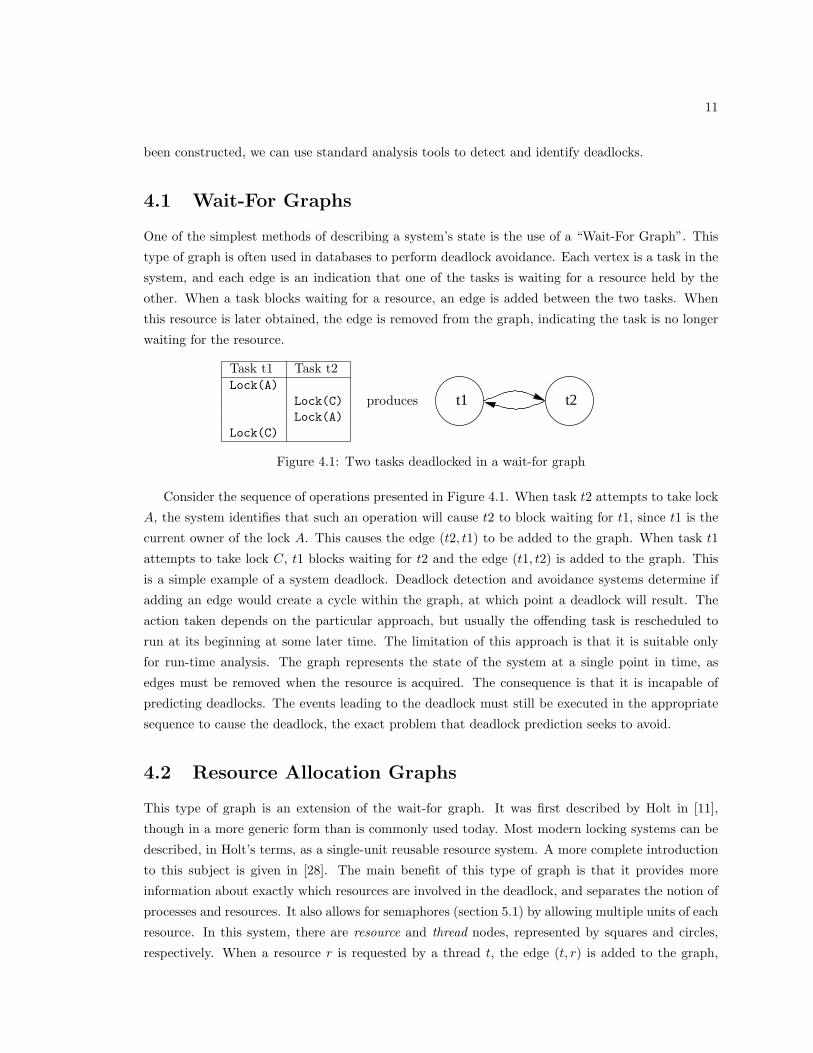
Task t1 Task t2Lock(A)
Lock(C)Lock(A)
Lock(C)
produces t1 t2
Figure 4.1: Two tasks deadlocked in a wait-for graph
Consider the sequence of operations presented in Figure 4.1. When task t2 attempts to take lock
A, the system identifies that such an operation will cause t2 to block waiting for t1, since t1 is the
current owner of the lock A. This causes the edge (t2, t1) to be added to the graph. When task t1
attempts to take lock C, t1 blocks waiting for t2 and the edge (t1, t2) is added to the graph. This
is a simple example of a system deadlock. Deadlock detection and avoidance systems determine if
adding an edge would create a cycle within the graph, at which point a deadlock will result. The
action taken depends on the particular approach, but usually the offending task is rescheduled to
run at its beginning at some later time. The limitation of this approach is that it is suitable only
for run-time analysis. The graph represents the state of the system at a single point in time, as
edges must be removed when the resource is acquired. The consequence is that it is incapable of
predicting deadlocks. The events leading to the deadlock must still be executed in the appropriate
sequence to cause the deadlock, the exact problem that deadlock prediction seeks to avoid.
4.2 Resource Allocation Graphs
This type of graph is an extension of the wait-for graph. It was first described by Holt in [11],
though in a more generic form than is commonly used today. Most modern locking systems can be
described, in Holt’s terms, as a single-unit reusable resource system. A more complete introduction
to this subject is given in [28]. The main benefit of this type of graph is that it provides more
information about exactly which resources are involved in the deadlock, and separates the notion of
processes and resources. It also allows for semaphores (section 5.1) by allowing multiple units of each
resource. In this system, there are resource and thread nodes, represented by squares and circles,
respectively. When a resource r is requested by a thread t, the edge (t, r) is added to the graph,
12
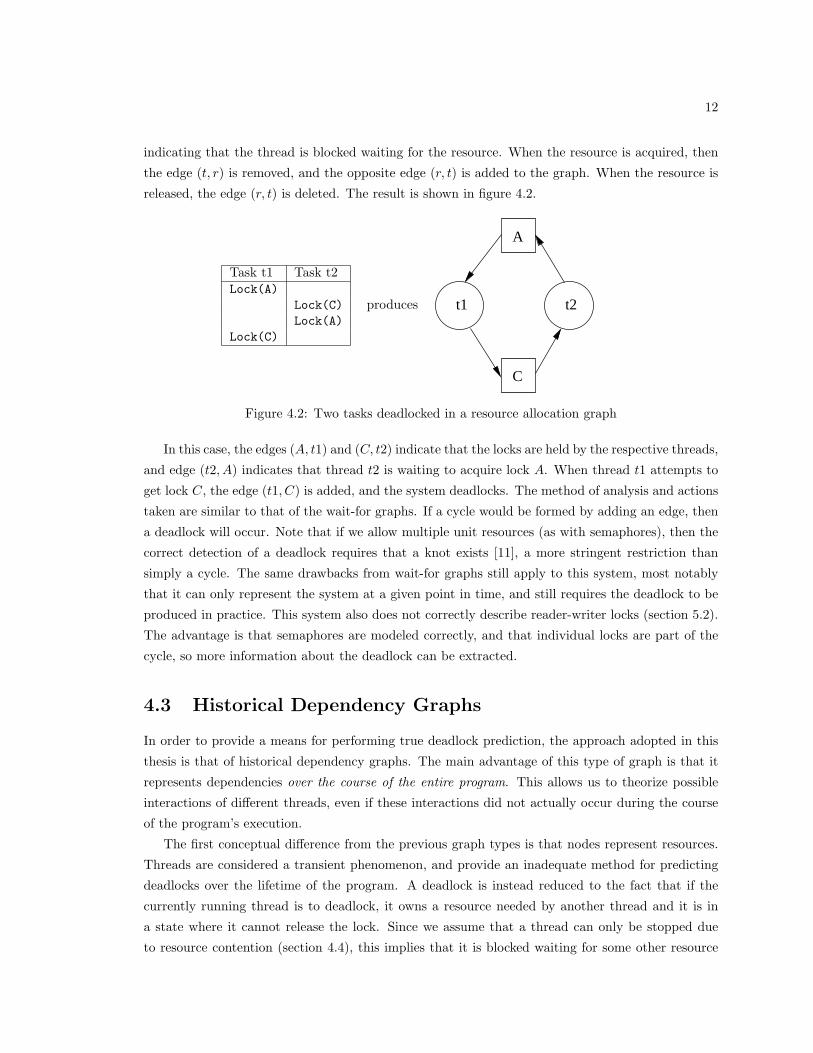
indicating that the thread is blocked waiting for the resource. When the resource is acquired, then
the edge (t, r) is removed, and the opposite edge (r, t) is added to the graph. When the resource is
released, the edge (r, t) is deleted. The result is shown in figure 4.2.
Task t1 Task t2Lock(A)
Lock(C)Lock(A)
Lock(C)
produces t1 t2
A
C
Figure 4.2: Two tasks deadlocked in a resource allocation graph
In this case, the edges (A, t1) and (C, t2) indicate that the locks are held by the respective threads,
and edge (t2, A) indicates that thread t2 is waiting to acquire lock A. When thread t1 attempts to
get lock C, the edge (t1, C) is added, and the system deadlocks. The method of analysis and actions
taken are similar to that of the wait-for graphs. If a cycle would be formed by adding an edge, then
a deadlock will occur. Note that if we allow multiple unit resources (as with semaphores), then the
correct detection of a deadlock requires that a knot exists [11], a more stringent restriction than
simply a cycle. The same drawbacks from wait-for graphs still apply to this system, most notably
that it can only represent the system at a given point in time, and still requires the deadlock to be
produced in practice. This system also does not correctly describe reader-writer locks (section 5.2).
The advantage is that semaphores are modeled correctly, and that individual locks are part of the
cycle, so more information about the deadlock can be extracted.
4.3 Historical Dependency Graphs
In order to provide a means for performing true deadlock prediction, the approach adopted in this
thesis is that of historical dependency graphs. The main advantage of this type of graph is that it
represents dependencies over the course of the entire program. This allows us to theorize possible
interactions of different threads, even if these interactions did not actually occur during the course
of the program’s execution.
The first conceptual difference from the previous graph types is that nodes represent resources.
Threads are considered a transient phenomenon, and provide an inadequate method for predicting
deadlocks over the lifetime of the program. A deadlock is instead reduced to the fact that if the
currently running thread is to deadlock, it owns a resource needed by another thread and it is in
a state where it cannot release the lock. Since we assume that a thread can only be stopped due
to resource contention (section 4.4), this implies that it is blocked waiting for some other resource

13
owned by a thread that can’t release it. An edge (r1, r2) indicates that at some point during the
program’s execution, lock r2 was owned when lock r1 was taken. This is the dependency modeled
by the graph. Any number of threads may generate this dependency (identifying the source of the
dependency is outlined in section 4.6), and it can occur many times during the course of the program.
No matter how many times it occurs, it is represented by a single edge in the graph. The important
fact is that the dependency exists, not how many times it occurred.
In order to generate such a graph, data needs to be processed in a time-ordered event stream,
where each event is associated with a given thread. Each thread maintains a list of all currently
held resources. When a thread acquires a new resource, a dependency is added (if it doesn’t already
exist) between the new resource and all currently held resources. When a resource is released, it is
removed from the thread’s list of currently held locks. During the course of the system’s execution,
every possible dependency is recorded in the graph. This is shown in figure 4.3.
Thread t1 Thread t2 Graph
Lock(C) C
Lock(A)
A
C
Lock(B)
A B
C
Unlock(B)
A B
C
Unlock(A)
A B
C
Lock(B)
A B
C
Lock(A)
A B
C
Figure 4.3: Three locks in a historical dependency graph
Note that the threads do not deadlock in the situation shown here. But given the right circum-
stances, there is potential for a deadlock in this schedule. It is possible for thread t1 to hold locks

14
A and C and thread t2 to hold just B, at which point both threads will deadlock. This schedule
is shown in figure 4.4. The main benefit is that this deadlock didn’t actually have to be created in
practice. These two threads could have run at vastly different times so there was no possibility of
deadlock. Implicit in the assumptions about concurrency (section 4.4) is the fact that these threads
could have been scheduled to run in such a way as to cause a deadlock.
Thread t1 Thread t2Lock(C)
Lock(B)Lock(A)Lock(B)
Lock(A)
Figure 4.4: Basic deadlock schedule
The second feature of the graph is that the deadlocks are reduced to dependencies between locks,
rather than processes. It doesn’t matter how many processes acquire A and then B; all that matters
is that somewhere this dependency exists. The fact that lock A is taken in between locks C and B
does not diminish the fact that there exists a dependency between B and C.
4.4 Concurrency Assumptions
In order to make the structure and analysis of the graph correct, it is necessary to make several
assumptions about the concurrent nature of the system being analyzed. The first assumption is
that it is a preemptive system with some type of pseudo-arbitrary scheduler. Any sequence of
events can be preempted, allowing any number of other threads to execute. In reality, there are
scheduling constraints on many systems, such as thread priorities and realtime threads. Even with
threads of different priorities, priority inversion (where a lower priority thread is temporarily raised
because it owns a resource needed by a higher priority thread) can induce a different schedule. In
the general case, the schedule is effectively arbitrary. The implication is that there is no sequence
of locking events that can be considered atomic. If there are such operations in the system, then it
the responsibility of the data source to model these operations as a single locking operation.
The second assumption is that there can be any number of threads running the same procedures
at any time. In many systems, there can be only one thread that executes a certain sequence of
operations. For highly concurrent systems such as those that we are trying to model, we assume
that this is not true. The only time when this can cause inconsistencies in the data is when a thread
is predicted as causing a deadlock through some scheduling interaction with itself. This is already
an unlikely case, and is usually easily identified by the programmer as not a deadlock. Since the
number of these threads is very small, and the chances of the deadlock occurring with the same
thread are unlikely, this is a valid assumption. The alternative, detecting when multiple copies of
the same thread are running at the same time, is impractical and reduces the scope of the deadlock
predictions.

15
The final assumption is that locks are released from the same thread that acquired them. This
is the case with any well-organized locking scheme, so it should not be an issue with the majority of
systems. If a lock release is missed because it was recorded as happening from another thread, then
the original lock will still be assumed to be held, and false dependencies will be created for each new
lock acquired. If, for some reason, the locking strategy allows for this sort of behavior, it is up to
the data gathering source to ‘spoof’ the holder of the original lock in order to make it seem like it
was released from the original thread.
4.5 Deadlock Detection
Detecting deadlocks in a historical dependency graph is a relatively simple process. A deadlock is
identified by a cycle within the dependency graph. This can already be seen with the example in
figure 4.3, but a more interesting example with three threads is shown in figure 4.5. Note that in
this figure, the notion of a universal time line is not shown in the interaction of the three threads,
since we assume that the individual events can happen at any point. This particular deadlock is
very difficult to produce in practice, but shows up as an easily detectable cycle in the dependency
graph.
Thread 1 Thread 2 Thread 3Lock(A) Lock(B) Lock(C)Lock(B) Lock(C) Lock(A)
produces
A B
C
Figure 4.5: Three way deadlock in a historical dependency graph
This analysis depends on several assumptions, and only detects the possibility of a deadlock.
Given our assumption of maximum concurrency, for any given edge (r1, r2), we have to assume
there can be a thread that owns lock r2 and is waiting for r1. This assumption generalizes to an
arbitrary path in the graph. For any path P , it can then be assumed that for any vertex Pi, there
can be a thread that owns lock Pi+1 and is waiting to acquire lock Pi. If the same lock appears twice
in a path, it is possible to have threads blocked on each intermediate vertex, but unable to continue
because the first thread is (by the transitive nature of dependency) blocked waiting for itself.
These assumptions made by the analysis can falsely identify deadlocks in theory, though they
are correct for nearly all deadlocks typically found in practice. For one thing, the assumption that
there can be multiple threads running the same code at a given time is not always true. This means
that conflicting actions taken by a single thread can be erroneously identified, as in figure 4.6.
If there are two threads running this same code, then there is the potential for the two threads
to deadlock. If there is no other thread contending for both A and B at the same time, and this

16
ThreadLock(A)Lock(B)Unlock(A)Lock(A)
produces A B
Figure 4.6: Potential deadlock misidentified
is the only thread in the system that executes this code, then there is no possibility of deadlock.
In reality, most concurrent systems can have any number of threads running the same procedures,
which is especially true of kernel code. Additionally, this can still deadlock if another thread ever
takes both A and B, regardless of the order.
Another possible scenario is one in which the offending actions are enclosed by some higher-order
locking principle, which may either be a lock in the system, or some interaction not capable of being
described by the data source. For example, consider the two different cases in figure 4.7.
Thread 1 Thread 2Lock(A) Lock(A)Lock(B) Lock(C)Lock(C) Lock(B)
Thread 3 Thread 4Lock(A) Lock(A)Lock(B) Unlock(A)Lock(C) Lock(C)
Lock(B)
both produce
A B
C
Figure 4.7: Identical graphs from different sources
If no other threads ever lock both B and C, then there can never be a deadlock between threads
1 and 2. This is because the common lock A is needed in order to acquire both of these locks,
superimposing a critical section on their access. This enforces an artificial scheduling constraint
that is not detectable during graph construction. The interaction of threads 3 and 4, however, does
allow for a deadlock. The difference is that the scheduling constraint has been removed. In either
case, a potential deadlock will be reported, and it is up to the programmer to discern between the
two different cases. In reality, it is unlikely to see the first situation, because with the overarching
critical section lock, there is no reason to lock B and C in the opposite order. It is also unlikely that
both B and C are never acquired anywhere else. While it cannot deadlock, this behavior should not
occur in a typical system.
4.6 Metadata
Since the nodes of the graph are only resources, the original information about where the depen-
dencies were generated in the system is lost. From the basic form of the graph, it is impossible

17
to tell where or when the original events occurred, only that they happened in such a way as to
generate the edge dependencies. Unlike the wait-for graphs and resource allocation graphs, which
allow the system to stop processes in real-time as they are about to cause a deadlock, the deadlocks
predicted by this scheme don’t occur. In order to analyze deadlocks effectively, we need to be able
to identify all possible sources of each dependency involved in the cycle. This means that additional
metadata must be kept in the graph in order to make identifying the deadlock useful. This is done
by associating some sort of snapshot of the current thread (typically in the form of a stack trace)
with each locking event. When a new lock is added to the list of currently held locks, the point at
which is was acquired is remembered by the graph construction system. Whenever a dependency is
created, the construction algorithm checks to see if the pair of events created by the newly acquired
lock and the previous lock is associated with the given edge. If not, then this pair is attached to
the edge, so later it can be used to determine how the dependency way generated. For example,
consider figure 4.8.
Thread t1 Thread t21 Lock(A) 1 Lock(B)2 Lock(B) 2 Lock(A)3 Unlock(B) 3 Unlock(A)4 Lock(B) 4 Unlock(B)5 Unlock(B)6 Unlock(A)
produces
B
A
(t1:1,t1:2)(t1:1,t1:4)
(t2:1,t2:2)
Figure 4.8: Metadata kept during graph construction
In this example, the lock event pairs are shown next to each edge in the graph. The first element
of the pair is where the first lock (the destination of the edge) was acquired. The second element is
where the second lock (the source of the edge) was acquired. Note that in this example, the data
that is attached to each event is the owning thread and line number in the example source. In a real
system, this would be a stack trace detailing exactly where the event occurred during execution.
Also note that there can be more than on pair of events associated with each edge, as demonstrated
with the edge (A,B). In this case, that dependency exists in two different places, but there is only
one edge. Each edge can therefore have any number of these lock event pairs. Once a cycle is found,
these lock event pairs are used to display the source of the dependency to the programmer in a
meaningful way.

Chapter 5
Locking Specifics
In the abstract sense, a historical dependency graph represents dependencies between resources
shared by different threads. The only required features of these resources is that there is a potential
for the requesting thread to be stopped when an attempt is made to acquire the lock. Traditionally,
this is represented as a a mutually exclusive lock which can be owned by only a single thread. If a
thread tries to acquire a lock that is held by another thread, it will be stopped until such a time
when it can acquire the lock.
This view describes only the most basic locking mechanisms that are present in modern systems.
There are different primitives, methods of accessing them, and ways in which events can be modeled
as locks. Up until this point, the locks have been dealt with as abstract named resources. In this
chapter the specifics of how real world implementations of various locking ideas can be translated
into the appropriate resource-dependent form needed to construct the graph. Example functions are
shown for the C language using the POSIX threads library, the Linux kernel, and the Solaris kernel.
5.1 Mutually Exclusive Locks and Semaphores
The most basic lock is a mutex. The mutex is a specific form of the semaphore, which allows for
an arbitrary number of threads to have access to the resource at the same time. The mutex is a
semaphore that allows only a single owning thread. Regardless of the number of threads that are
allowed access to the mutex or semaphore, it is presumed that any operation can block if there enough
owners of the resource, or else why have a lock at all. The common functions used to manipulate
these primitives are shown in table 5.1. Note that for kernel implementations (and newer POSIX
implementations), there are two types of locks, adaptive locks and spin locks. With spin locks, the
thread does not actually get suspended by the scheduler, it merely waits until the lock is free, tying
up the processor upon which it’s scheduled until the lock is released. This is equivalent to being
blocked, because it is assumed that if the system is using spin locks, then it is a multi-processor
system or code executing in user mode. Other threads will still be capable of running, and the
controlling process will behave exactly as if it were stopped. This functionality has been added to
18

19
POSIX threads in the IEEE 1003.1-2001 standard [12].
POSIX Linux Kernel Solaris KernelLock pthread mutex lock down mutex enter
pthread spin lock spin lock lock setlock set spl
Unlock pthread mutex unlock up mutex unlockpthread spin unlock spin unlock mutex destroy
spin unlock wait lock clearlock clear splx
Table 5.1: Common mutex and semaphore locking functions
5.2 Reader-Writer Locks
An extension of the basic semaphore is that of the reader-writer lock, in which there can be multiple
readers that hold the lock, but only one writer. If there are no waiting writers, then a read attempt
will immediately acquire the lock, regardless of how many other readers currently own the lock. If a
thread owns a write lock, or is blocked waiting for a write lock, then the read attempt will block until
the writer has released the lock. A write attempt will block if any thread owns the lock (regardless of
the type of lock currently held). This type of lock is simple to integrate into the dependency graph
based on our assumptions about concurrency. Given a reader-writer lock, any write attempt can
always block. In a highly concurrent system, we assume that at any given point in time there may
be a writer that owns the lock, or is waiting to acquire it. This means that any read attempt can
also block. Therefore, any operation, whether a read attempt or a write attempt, has the possibility
of blocking. The common functions to manipulate these locks are shown in table 5.2. Note that the
POSIX functions are not part of the original standard, but the IEEE 1003.1-2001 standard [12].
POSIX Linux Kernel Solaris KernelLock pthread rwlock rdlock down read rw enter
pthread rwlock wrlock down writeUnlock pthread rwlock unlock up read rw exit
up write
Table 5.2: Common reader-writer lock functions
Since read lock can always block, the analysis catches the common bug of recursively acquiring
a read lock. Under normal circumstances this will have no effect, since the second read lock will
silently succeed. Typical implementations do not keep track of which threads own read locks, only
the number of active readers, so it is impossible to tell if a thread that is attempting to acquire
the lock already has a read lock. If an intervening write request were to occur, the thread would
deadlock with itself when it attempted to get another read lock. The writer will also be blocked
waiting for the the original thread to release the read lock, resulting in a deadlock. This situation
is shown in figure 5.1. Note that there is a cycle between lock A and itself.

20
ThreadRead(A)Lock(B)Unlock(B)Read(A)
producesA B
Figure 5.1: Recursive reader-writer lock
5.3 Non-blocking Locks
In most locking systems, locks can be acquired by methods that do not block. These functions
attempt to acquire the lock (sometimes continuously for a given time period), but if they are unable
to acquire the lock, then they return to the calling function with a status code indicating that the
lock could not be obtained. The common functions are shown in table 5.3. These functions present
some difficulty because they cannot possibly be a point of deadlock, since the thread cannot block
while waiting for one of these functions to complete. It is possible for future events to depend on
the lock being owned, however.
POSIX Linux Kernel Solaris Kernelpthread mutex trylock down trylock mutex tryenterpthread spin trylock spin trylock lock trypthread rwlock tryrdlock rw tryenterpthread rwlock trywrlock
Table 5.3: Common non-blocking lock functions
In order to deal with this problem effectively, non-blocking acquisitions have to be identified in
the data source. When one of these events is processed, the target lock is added to the thread’s
list of currently owned locks, but no dependencies are created to currently held locks. By adding it
to the known lock list, subsequent locking events will still create dependencies to the non-blocking
lock. This is outlined in figure 5.2. Note that there is no dependency between B and A, but there
still is the possibility of a deadlock between B and C, even though B is acquired in a non-blocking
fashion.
Thread 1 Thread 2Lock(A) Lock(C)Trylock(B) Lock(B)Lock(C)
produces
A B
C
Figure 5.2: Non-blocking locks

21
5.4 Interrupts as Locks
In a operating system kernel, interrupts play a crucial role in the system. Their asynchronous nature
makes them difficult to analyze, especially in highly preemptive kernels such as Solaris, where locks
can be taken at raised interrupt levels.
In an operating system, an interrupt is an asynchronous signal passed to the kernel, usually from
a hardware device (although software interrupts are also possible). Each interrupt is associated with
a number, called the interrupt level. There can be any number of different interrupt levels depending
on the processor and operating system. The Solaris kernel (on SPARC platforms), for example, has
15 interrupt levels. When an interrupt occurs, the operating system passes the interrupt off to
a special handler for that level. The mechanism used to accomplish this differs from system to
system, but the mechanics do not affect the theory. In order to prevent multiple interrupts of the
same level from occurring at the same time, each processor maintains the notion of the current
“interrupt priority level,” or IPL (also sometimes abbreviated PIL, processor interrupt level). When
the IPL is set to a non-zero level, then no interrupts of an equal or lower level will be serviced on
that processor (they are instead queued and handled when the IPL is later lowered). If the IPL
is 10, then no interrupts of levels 1-9 will be serviced. When an interrupt is handled, the IPL is
automatically set to the level of the current interrupt. One important fact about the IPL is that it
is local to a specific processor. In a multiprocessor system, one processor may have an IPL of 10 and
therefore be incapable of servicing interrupts below that level, while another processor may have an
IPL of 0, and can still receive interrupts.
By themselves, interrupts do not present much of a problem in the area of deadlock prediction.
Interrupts can be modeled as traditional threads, since the interrupt handler’s execution can be seen
as a very short lived thread. The actual mechanics of executing an interrupt handler are somewhat
tricky, since it involves borrowing the current stack from whatever thread is executing. Under the
Solaris model when an interrupt handler blocks on a synchronization primitive, it is converted into a
full-fledged thread. This means that they can be analyzed in the same fashion as any other threads
in the system. Because of our concurrency assumptions, there is no difference between an interrupt
thread and a normal thread.
Function IPL Requiredbiowait() 7cv timedwait() 10kmem alloc(KM SLEEP) 7
Table 5.4: Interrupt-Dependent functions in the Solaris kernel
This situation becomes complicated with the introduction of interrupt-dependent functions.
There are various functions throughout the kernel that implicitly require interrupts of a certain
level to be serviced in order for the function to complete. Some of these functions are shown in table
5.4.
For example, the biowait function is used to wait for binary I/O operations to complete. In

22
order to do this, the hardware device being used (whether it be a network card or a hard disk)
signals the operating system that the operation is completed via an interrupt. The kernel then runs
the appropriate handler (which can be at an IPL of up to 7), which calls the I/O completion routines
that signal the caller of the biowait function that the operation is complete. Until this interrupt
is received, the caller of biowait is effectively blocked, though it is not blocked on a traditional
synchronization primitive. If the processor cannot service interrupts of level 7 or below, then the
function will never return, and the thread will stop. If an interrupt handler of level 7 or higher is
blocked on a resource that it cannot get (perhaps because the thread calling biowait holds it), then
the system is deadlocked, since the interrupt handler can never complete. This example is shown in
figure 5.3.
Thread Interrupt Handler NotesLock(A)
Receive Level 10 Interrupt IPL is now set at 10Lock(a) Interrupt Handler now blocked (IPL
remains at 10)
biowait() Requires interrupts of level 7 in orderto return
blocked blocked Level 7 interrupts cannot be received;system is deadlocked
Figure 5.3: Deadlocked on the biowait() function
Similarly, the there is a special clock handler that runs at IPL 10 on a regular basis and performs
various routine tasks. One of the additional synchronization primitives that hasn’t been mentioned
yet is the condition variable. A condition variable isn’t like most other synchronization primitives,
in that it is not something that is owned or acquired by a thread. Instead, a thread waits for a
signal to be passed from another thread via the condition variable. One of the methods of accessing
these primitives is through the use of a function with a timeout. If no signal is received within the
timeout period, then the function returns anyway indicating that it did not receive a signal. The
condition variables in the kernel are implemented around this clock handler when trying to do a
timed operation. If cv timedwait is called, then the clock handler must be able to run in order
to signal to the calling function that the given timeout has expired. Otherwise, the function will
never return (unless the condition variable is actually signalled), and the purpose of the function
will be destroyed. This is not truly a deadlock in any traditional sense, since it is still possible for
the condition variable to be signalled from another thread, but until this point, the clock interrupt
handler will be unable to run and the whole system will be impaired.
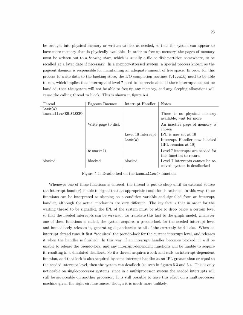
The most complicated example, and the most difficult to produce in practice, is if kmem alloc is
called with KM SLEEP. This is what is called a sleeping allocation. This informs the memory system
that if there is no memory available, then the thread should be put to sleep until such a time as
more memory can become available. In a system using virtual memory (which is almost all modern
operating systems today), memory is divided up into larger chunks called pages. These pages can
23
be brought into physical memory or written to disk as needed, so that the system can appear to
have more memory than is physically available. In order to free up memory, the pages of memory
must be written out to a backing store, which is usually a file or disk partition somewhere, to be
recalled at a later date if necessary. In a memory-stressed system, a special process known as the
pageout daemon is responsible for maintaining an adequate amount of free space. In order for this
process to write data to the backing store, the I/O completion routines (biowait) need to be able
to run, which implies that interrupts of level 7 need to be serviceable. If these interrupts cannot be
handled, then the system will not be able to free up any memory, and any sleeping allocations will
cause the calling thread to block. This is shown in figure 5.4.
Thread Pageout Daemon Interrupt Handler NotesLock(A)kmem alloc(KM SLEEP) There is no physical memory
available, wait for more
Write page to disk An inactive page of memory ischosen
Level 10 Interrupt IPL is now set at 10Lock(A) Interrupt Handler now blocked
(IPL remains at 10)
biowait() Level 7 interrupts are needed forthis function to return
blocked blocked blocked Level 7 interrupts cannot be re-ceived; system is deadlocked
Figure 5.4: Deadlocked on the kmem alloc() function
Whenever one of these functions is entered, the thread is put to sleep until an external source
(an interrupt handler) is able to signal that an appropriate condition is satisfied. In this way, these
functions can be interpreted as sleeping on a condition variable and signalled from an interrupt
handler, although the actual mechanics are very different. The key fact is that in order for the
waiting thread to be signalled, the IPL of the system must be able to drop below a certain level
so that the needed interrupts can be serviced. To translate this fact to the graph model, whenever
one of these functions is called, the system acquires a pseudo-lock for the needed interrupt level
and immediately releases it, generating dependencies to all of the currently held locks. When an
interrupt thread runs, it first “acquires” the pseudo-lock for the current interrupt level, and releases
it when the handler is finished. In this way, if an interrupt handler becomes blocked, it will be
unable to release the pseudo-lock, and any interrupt-dependent functions will be unable to acquire
it, resulting in a simulated deadlock. So if a thread acquires a lock and calls an interrupt-dependent
function, and that lock is also acquired by some interrupt handler at an IPL greater than or equal to
the needed interrupt level, then the system can deadlock (as seen in figures 5.3 and 5.4. This is only
noticeable on single-processor systems, since in a multiprocessor system the needed interrupts will
still be serviceable on another processor. It is still possible to have this effect on a multiprocessor
machine given the right circumstances, though it is much more unlikely.

24
In order to make the analysis robust, each interrupt level is modeled as depending on the next
lower interrupt level being “owned”. If a processor is at IPL 7, it implies that interrupts of level 7
and below (by transitive dependency) are unserviceable. This is done at the beginning of the data
set by means of implicit dependencies - arbitrary relationships that do not actually appear in the
data itself.
One common example in the Solaris kernel is with kmem alloc and the interactions of the clock
handler, as described previously. The clock handler runs at IPL 10, and acquires the process lock
(p lock), among other locks, in order to calculate process usage statistics. Therefore, if a thread
acquires p lock and then does a sleeping allocation (with KM SLEEP), this could potentially deadlock
the system in heavy-memory situations. This particular bug is extremely difficult to produce in
practice, often requiring runs of many days in order to produce. By modeling the interrupts as
locks, the deadlock can be found simply by running a coverage test once. This example is shown in
figure 5.5. Note the implicit dependencies between the various interrupt levels.
Thread Clock InterruptLock(p lock) Lock(p lock)biowait()
produces
IPL7
p_lock
IPL8 IPL10IPL9
Figure 5.5: Interrupt-Dependent Functions
5.5 Dynamic Memory
In almost every system, dynamic memory allocation is used for some data structures. For most
concurrent systems, these data structures typically contain synchronization primitives in order to
share the contents of the data structure. This presents a problem, since the memory address (whether
virtual or physical) is not sufficient to uniquely identify a lock in the system over the course of the
entire execution. Two logically independent locks may end up sharing the same physical address at
different points in time, depending on the way in which they are allocated. One method of avoiding
this situation is to keep track of lock allocations and deallocations at run-time, and then assign
unique IDs to each lock regardless of the address used. Without extensive modifications to the
programming interface (a violation of the stated design goals), it would require maintaining a large
amount of metadata at run time. This would affect the runtime performance in an unacceptable
way.
In order to deal with this situation, each lock is referenced by a memory address, and then a
separate “generation count” is maintained while the graph is being built in order to differentiate
between logically different locks sharing the same address. In order to determine when the generation

25
count must change, any events which free a range of memory are recorded in the event stream. The
runtime gathering tools are not responsible for detecting whether these events actually affect any
locks. While the graph is being constructed, a global list of all known locks is maintained, including
their generation counts. When a memory free event is processed, this global list is checked to see if
any known locks fall within the specified range. Each of these locks is then checked to see if it has
been accessed since the last time the generation count was updated. If there were no events using
the lock, then the lock is ‘clean’, and there is no need to update the generation count. If the lock is
dirty, then the generation count is increased by one, and the lock is marked as clean. Whenever any
lock is used, it is internally translated to a (address, generation) pair according to the global table
before it is passed on to the rest of the graph construction algorithm. This is shown in figure 5.6.
ThreadA = Alloc()Lock(A)Lock(B)Unlock(B)Unlock(A)Free(A)A = Alloc()Lock(B)Lock(A)
produces
B
A:0 A:1
Figure 5.6: Dynamically allocated locks
This assumes that the lock A is an address returned from a dynamic allocation routine, and
that the second time the routine returns the same address just freed. If the address was the single
identifying characteristic of a lock, then this would be misidentified as a deadlock. Notice that the
second time the lock is used, the generation count has increased.
Under most systems, it is possible for a programmer to release memory for a lock while it is still
locked. In general, this is poor programming practice, but it doesn’t mean that it can’t happen. In
order to combat this lazy programming style, it is necessary to ‘spoof’ the release of any lock that
is freed in a locked state. Unfortunately, the multithreaded way in which the graph is constructed
(section 7.1) makes it impossible to know whether a lock is being held at the time the free event is
processed. The solution is to spoof a release event for the given lock on every known thread in the
system. Since a release event does nothing if the lock isn’t currently held, this does not affect the
correctness of the construction.

Chapter 6
Gathering Data
Since the analysis of the dependency graph is independent of the system that was used to produce
the data, the analysis program can be kept separate from the data gathering program. This creates
a cross-platform, source-independent system for analysis of potential deadlocks. The program can
be deployed on a large variety of systems, such as user programs on various operating systems,
operating system kernels, and distributed systems. The locking events are streamed to a common
file format, which is then fed to the generic analysis program in order to construct the graph. This
chapter details the structure of this file, and the different data sources that can be used.
6.1 File Format
In order to make generic analysis possible, the locking events must be streamed to common data file
format. The basic format is a time-ordered sequence of generic locking events. Since we are dealing
with potentially very large data sets (on the order of hundreds of millions of records), a compact
binary form is needed. While it may be more portable to use a text-based standard such as XML,
this would make the file extremely large and severely cripple the speed at which the file could be
processed. The binary format is made slightly more complex by the fact that the primitives in the
system (locks, threads, and symbols) are not a fixed size, and can vary from system to system. The
records are all variable sized, and a header at the beginning of the file indicates the size of each
primitive type. These primitives are logically limited to sizes that are a multiple of 4 bytes, since
we are typically dealing with addresses. This restriction could be removed at the expense of more
complex processing code. In order to indicate what the primitive sizes are, there is an initial header
at the beginning of every file, shown in figure 6.1.
Magic Number Version NumberLock ID Size Thread ID SizeSymbol Size Endianness
Figure 6.1: File information header
26

27
The magic number is used to identify that the file is actually a data file, and the version in-
formation is used to match the data file to the appropriate analysis program. The endianness flag
determines whether the data in the file is stored in big endian (most significant bit first) or little
endian format. The analysis program can convert between the two during processing, but if the data
is in the native system’s endianness this translation can be avoided. The remaining fields of the
header describe the size of each of the primitives used in the system. These primitives are described
in further detail in section 6.2. After this general header is any number of variable-sized records.
6.2 Source Independent Records
Each record contains some information about the nature of the lock event, and is built from three
locking primitives. These primitives are an abstract value that are used to identify resources in the
system.
• Lock ID - This uniquely identifies a lock in the system (discounting different generations of the
same ID). For user programs this is the virtual address of the lock in the program’s memory. For
operating system kernels, this can either be a virtual address or a physical address, depending
on how the kernel address space is setup. For more complicated systems (such as distributed
systems), a more complex scheme could be devised. Note that it is assumed that locks are
laid out linearly in the ID space, so that when a generation count increment event (freeing of
dynamic memory) occurs, it will update the generation counts of of all locks sharing IDs in
the given range.
• Thread ID - A unique identifier for a thread in the system. Most locking events are associated
with a given thread, so each thread needs to have a unique identifier throughout the execution
of the system. For a user program using POSIX threads, this is the identifier returned from
the pthread self() call. For a kernel, it is often not enough to use the address of the thread
structure in kernel memory to identify the thread, since this must be unique across the lifetime
of multiple threads. For the Solaris kernel, the only appropriate value to use is the t did field
of the kthread t structure, since it is guaranteed to be unique across the life of the entire
system.
• Symbol - Certain locking events can have symbols associated with them. This sequence of
symbols is used by the programmer to identify where in the program the event occurred when
the deadlock is later examined. These symbols are typically translated into symbolic strings,
which are easier to understand than the numerical values. For most systems, a symbol is an
address in the stack trace of a call. This address is translated into a string representing the
(symbol,offset) pair that the programmer can then use to determine where in the source code
the event occurred.
With these primitives, all possible locking events can be appropriately modeled. Some of these
records correspond to actual locking or memory events during the execution of the program, and

28
Second LockFirst Lock
2
1
Start Lock End Lock
Type Symbol Count Lock IDThread ID Symbol List4
Symbol Value Symbol Name
Symbol Definition
3
Generation Increment
Implicit Dependency
Lock Operation
Figure 6.2: Record types
other records are external to the execution of the program, and affect implicit dependencies or
the symbol table. The structure of each record is shown in figure 6.2. The gray dividers indicate
variable-sized fields. A more detailed description of each record type follows.
• Implicit Dependency - This is a special record that sets up an absolute dependency between
two locks in the graph. This dependency is not associated with a particular thread or point
in time. Normally, these implicit dependencies are used at the beginning of the data source
to describe a relationship that is not present in the data. An example of this is modeling
interrupts as lock, as described in section 5.4. The only fields in the record are two lock IDs,
where the second depends on the first.
• Generation Increment - A record indicating a memory free event. This event is not associ-
ated with a thread, since the lock ID space is shared by all threads. It still must be ordered in
time with the rest of the events, since it affects the generation count of all subsequent locks.
The two fields of the record are the starting and ending lock IDs which denote the range of
memory to check for changes to generation counts. See section 5.5 for more information. The
ending lock ID is non-inclusive, so it checks all the memory until just below the second lock
ID.
• Symbol Declaration - Used to associate a numerical symbol with a plaintext string, in order
to make results more readable. This adds an entry to the global symbol table, which is used
when displaying results (section 7.3). The record includes the length of the string, padded
out to 4 bytes so that the records always lie on word-aligned boundaries. The string itself is
null-terminated to indicate the end of the string (extra padding is ignored).

29
• Lock Operation - This is the typical data record, operating on a specific lock in a given
thread. There are several types of this record, indicated by an enumerated field. The possible
types are BLOCKING, NONBLOCKING, or RELEASE. The difference between blocking and
nonblocking lock acquisitions is described in section 5.3. Each record is associated with a
specific thread, indicated by a thread ID, and each record can have any number of symbols
attached to it. As described previously, these symbols are used to identify where the event
occurred after the fact. For release events, the symbols are ignored during graph construction,
so there is no need to attach symbols.
An example translation between a POSIX thread program and the corresponding locking events
is shown in figure 6.3. Note that in this case, the ‘symbols’ being used are the line numbers of the
program. More typically, there would be multiple symbols associated with each event, where each
symbol was an address in the stack trace at the time of the event.
Source Code1 pthread mutex t *a;2 a = malloc(sizeof(*a));3 pthread mutex initialize(a,NULL);4 pthread mutex lock(a);5 pthread mutex unlock(a);6 free(a);
Event TranslationLock Operation
Type = BlockingLock ID = addr(a)Symbol List = (4)
Symbol Definition4 = “Line 4”
Lock OperationType = ReleaseLock ID = addr(a)
Generation IncrementStart = addr(a)End = addr(a) + sizeof(*a)
Figure 6.3: Translation from source code to events
6.3 Library Interpositioning
The most immediately obvious target for deadlock analysis is programs running in user mode in
an operating system environment. While it is possible to accomplish this through dynamic trac-
ing (section 6.4), there is already a mechanism for intercepting library calls built into most UNIX
systems. With a UNIX system and dynamically linked executables, it is possible to interposition
a custom library in between the program binary and a system library, using the LD PRELOAD envi-
ronment variable as demonstrated in figure 6.4. This can then be used to intercept system thread
calls [6]. Note that for this particular implementation, the data is streamed out to a file with the
name “lockgrab.pid,” where ‘pid’ is the process ID of the command. This can be controlled through
flags in the environment, but the actual specifics are not important. Once the library is preloaded,
the dynamic loader will resolve symbols originally targeted for the system shared library into the
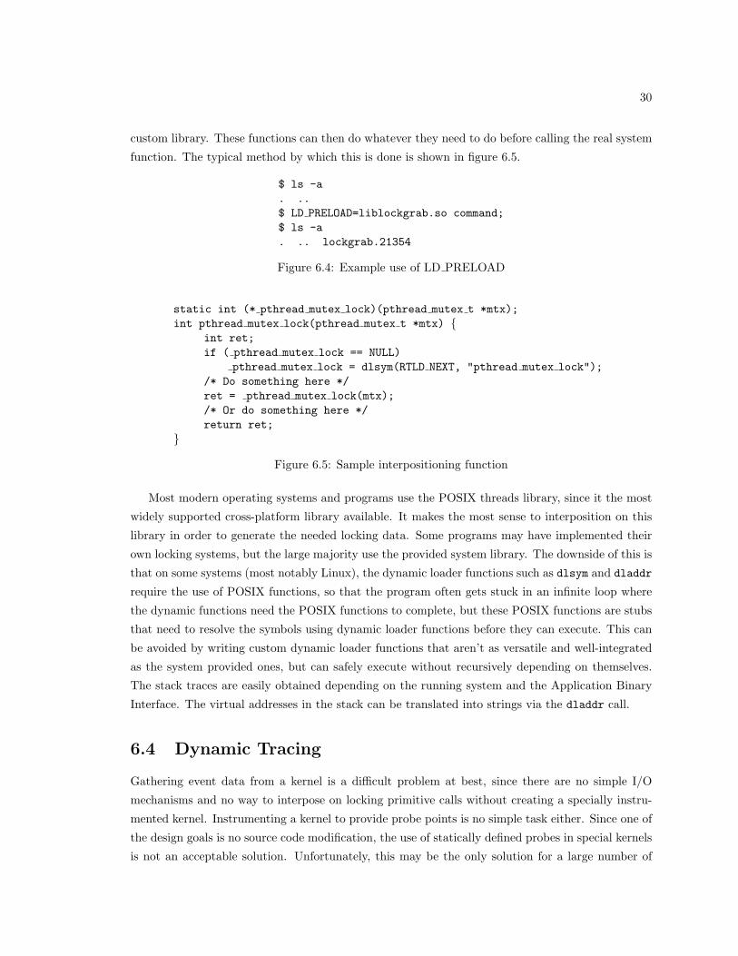
30
custom library. These functions can then do whatever they need to do before calling the real system
function. The typical method by which this is done is shown in figure 6.5.
$ ls -a. ..$ LD PRELOAD=liblockgrab.so command;$ ls -a. .. lockgrab.21354
Figure 6.4: Example use of LD PRELOAD
static int (* pthread mutex lock)(pthread mutex t *mtx);int pthread mutex lock(pthread mutex t *mtx) {
int ret;if ( pthread mutex lock == NULL)
pthread mutex lock = dlsym(RTLD NEXT, "pthread mutex lock");/* Do something here */ret = pthread mutex lock(mtx);/* Or do something here */return ret;
}
Figure 6.5: Sample interpositioning function
Most modern operating systems and programs use the POSIX threads library, since it the most
widely supported cross-platform library available. It makes the most sense to interposition on this
library in order to generate the needed locking data. Some programs may have implemented their
own locking systems, but the large majority use the provided system library. The downside of this is
that on some systems (most notably Linux), the dynamic loader functions such as dlsym and dladdr
require the use of POSIX functions, so that the program often gets stuck in an infinite loop where
the dynamic functions need the POSIX functions to complete, but these POSIX functions are stubs
that need to resolve the symbols using dynamic loader functions before they can execute. This can
be avoided by writing custom dynamic loader functions that aren’t as versatile and well-integrated
as the system provided ones, but can safely execute without recursively depending on themselves.
The stack traces are easily obtained depending on the running system and the Application Binary
Interface. The virtual addresses in the stack can be translated into strings via the dladdr call.
6.4 Dynamic Tracing
Gathering event data from a kernel is a difficult problem at best, since there are no simple I/O
mechanisms and no way to interpose on locking primitive calls without creating a specially instru-
mented kernel. Instrumenting a kernel to provide probe points is no simple task either. Since one of
the design goals is no source code modification, the use of statically defined probes in special kernels
is not an acceptable solution. Unfortunately, this may be the only solution for a large number of
31
platforms. A better solution is to use dynamic probe points, where probes are enabled at runtime
by rewriting the text code.
Very few systems like this exist, in part because it is a very difficult problem, and detailed
knowledge of a system’s assembly language and execution semantics is needed in order to implement
it correctly. More information on the semantics and difficulties of dynamic instrumentation can be
found in [33] [26] and [27]. A few tracing frameworks have existed for the Solaris kernel over the years,
including the deprecated VTrace and, more recently, TNF tracing [24]. These implementations still
rely on defining static disabled probes within the kernel, and any change in the probes requires a
re-compilation of the kernel. Limited lock information can be gathered on Solaris using the lockstat
utility [25], although this is not suitable for creating a robust implementation suitable for analysis.
A recent implementation of true dynamic kernel probes is KernInst, a dynamic trace facility for the
Sparc platform. For the kernel tracing done in this project, a specially instrumented Solaris kernel
was used, courtesy of Sun Microsystems’ Solaris Kernel Group.
Unfortunately, the selection of open-source tracing frameworks for the Linux kernel are wholly
inadequate for the type of tracing required by this project. The most promising is a combination of
the Linux Tracing Toolkit [33] and IBM’s DProbes facilities [16] [3]. Unfortunately, these systems
are still under development, and although they are largely functional, they do not provide enough
facilities to extract the necessary information from the Linux kernel. A number of tools exist for
doing Linux kernel profiling, such as SGI’s lockmeter [4] and kernprof [19], but these are intended
for performance monitoring, not generic event gathering.
It is also possible to use dynamic tracing for user space programs. This is potentially easier, since
the instructions can be changed to simply trap into the kernel on most platforms, although this still
requires extensive kernel modifications. Since reasonable functionality can already be achieved using
library interpositioning, dynamic tracing’s greatest benefit providing kernel-level tracing.
6.5 Other Possibilities
Since the data source gathering tools and the analysis tools are intentionally kept separate, there
is unlimited potential for the number of systems that the program can be applied to. The only
stipulation is that the system follows the assumptions and locking consistency outlined in section
4.4. Due to the scope of this project, it was unreasonable to pursue any more methods than the
library interpositioning and Solaris kernel tracing presented here. Some of the future possibilities
include java (or other language) based programs, distributed systems analysis, or the Linux kernel.
All of these systems can be modeled in the same way, as long as the data gathering tools are correctly
implemented.
Chapter 7
Analysis and Display of Results
In order to predict possible deadlocks from a given data source, we must first construct the historical
dependency graph, and then search for the necessary cycles. Because we are dealing with very large
data sets, the graph produced will be large and time-consuming to build. Therefore, not only
must the graph be built correctly, but it must be built in an efficient manner. Once the graph
is constructed, it then becomes necessary not only to detect the cycles within the graph, but also
to display the results in a meaningful manner. This chapter details some of the specifics of graph
construction and analysis.
7.1 Graph Construction
In recent years, multiprocessor machines have become more and more common. In order to satisfy
the design goals, the program must scale with additional processors. This implies that there must
be multiple threads running concurrently to produce the graph, cutting down construction time for
multiprocessor systems.
Unfortunately, since the data stream is time-ordered, and the generation count of locks is a global
property, there there must always be a single thread processing the data source. The existence of a
generation-count increment event can affect the interpretation of future events. This single thread
does only the minimal required work, which is maintaining generation counts for locks in the system
and passing on events to threads. Symbol definition records are handled by a special thread, but
all of the ‘normal’ locking events are localized to a specific thread. Rather than having a single
execution thread correspond to every thread structure in the data source, idea of a worker thread
is used instead, where each worker manages several data-source threads. The number of worker
threads created is directly related to the number of processors on the system.
Rather than having each worker share a common graph (which would require locking and increase
contention), there is a graph local to each worker. This has the benefit of creating lockless data
structures, but has the downside of increasing the memory footprint (since the same vertices and
edges may appear in multiple graphs) and forcing the implementation to merge all of the graphs
32

33
into a final representation. Due to the large number of events, the addition of vertices and edges will
be fairly common, suggesting that there will be a great deal of contention between worker threads
if they were to share a common graph. It makes more sense to perform one time-consuming merge
operation at the end of construction, rather than forcing workers to contend for common resources.
The edges and vertices are kept in dynamic hash tables, yielding approximately constant access
time. The lock event pairs (described in section 4.6) are maintained in a linked list for each edge,
since there will be relatively few cases where a dependency is established in multiple places. The
overall layout of the system is shown in figure 7.1.
The algorithm used to process the “normal” locking events is shown in figure 7.2, and runs locally
for each worker. Generation count increment and symbol definition events are handled separately.
In this algorithm, the thread parameter is the local thread structure, the graph parameter is the
worker-local graph, lock is the (address,generation) pair identifying the lock, operation is the type
of operation, and lockevent is a (address,generation,symbol list) tuple that can be used to identify
where the event occurred within the system.
Symbol Table
Global LockTable
Worker
Worker
GraphLocal
GraphLocal
Event Stream
Parser
Symbol Resolver
EventsPer−Thread
Structures
Figure 7.1: Graph Construction System
The global lock list and symbol table implementations are relatively straightforward. Every lock
that passes through the parsing thread is checked to see if it exists in the global list. This list is
an AVL tree, since whenever a generation count increment event is received, the entire range of
addresses must be checked. This makes a hash table unusable. The symbol table is simply a hash
table between symbol addresses and strings. Internally, the numerical addresses are used to identify
and compare symbols, but when the data needs to be printed out, the string translation is used.

34
ProcessThreadEvent(thread, graph, lock, operation, lockevent)1 if lock /∈ V ertices[graph]2 then V ertices[graph]← V ertices[graph] ∪ lock3 if operation = BlockingAcquisition4 then for ∀ l ∈ HeldLocks[thread]5 do if (lock, l) /∈ Edges[graph]6 then Edges[graph]← Edges[graph] ∪ (lock, l)7 e← e ∈ Edges[graph] such that e = (lock, l)8 if (LockEvent[l], lockevent) /∈ Events[e]9 then Events[e]← Events[e] ∪ (LockEvent[l], lockevent)
10 if operation = NonBlockingAcquisition ∨ operation = BlockingAcquisition11 then HeldLocks[thread]← HeldLocks[thread] ∪ lock12 l← l ∈ HeldLocks[thread] such that l = lock13 LockEvent[l] = lockevent14 if operation = Release15 then HeldLocks[thread]← HeldLocks[thread]− lock
Figure 7.2: Per-thread event processing algorithm
7.2 Cycle Detection
In order to detect cycles, a modified depth-first search algorithm is used. In this algorithm, every
vertex is marked as either unknown, visited, or active. Initially, all vertices are marked as unknown.
Then, for each unknown vertex, we push it onto a stack, and mark the vertex as active, indicating
that it is currently in the stack. We then look at each outgoing edge from the vertex. If the
destination vertex is active, then we have found a cycle. If the destination vertex is unknown, then
we continue with the algorithm recursively with the next destination vertex. If the vertex is visited,
then we ignore it. This prevents us from inadvertently searching down paths that we have already
seen. Once all of the neighbors have been visited, the current vertex is removed from the stack and
marked as visited. This algorithm is shown in figure 7.3, and is called on every vertex in the graph
in order to find all possible cycles.
FindCycle(graph, vertex, stack)1 if mark[vertex] = VISITED2 then return3 if mark[vertex] = ACTIVE4 then print cycle5 if mark[vertex] = UNKNOWN6 then push vertex on stack7 mark[vertex]← ACTIVE8 for ∀ e ∈ outgoing[vertex]9 do FindCycle(graph, end[e], stack)
10 pop vertex from stack11 mark[vertex]← VISITED
Figure 7.3: Cycle detection algorithm

35
This algorithm fails for certain cases of multiple cycles. Specifically, if two vertices are both part
of two different cycles, then only one of the cycles will be found. This is demonstrated in figure 7.4.
The smaller 3-vertex cycle is detected, but then the larger cycle is not found because one of the
vertices has already been marked as visited. This is not a problem for two reasons. First, the system
being analyzed is expected to be largely correct, since most of the common deadlocks would have
been produced through normal testing. Therefore, the graph is going to be largely acyclic, with only
a few cycles to be found. Second, the majority of cycles will contain only two vertices. The most
common deadlock by far is a mixed dependency between two threads. Any cycle of more than two
vertices implies multiple threads with cascading dependencies, an unlikely scenario. Combined with
the low probability that two vertices are part of two different cycles, this is an unlikely situation.
The simplicity and speed of the algorithm are more important.
Current Vertex
Unknown
Visited
Active
Missed Cycle
Figure 7.4: Cycle missed by detection algorithm
7.3 Displaying Meaningful Data
Once a cycle has been found, it becomes important to display the cycle in a meaningful way to
the user of the program. Section 4.6 describes the method by which individual events are stored
with each edge. We go through each edge in the cycle and print out the event information about
when each lock was acquired. This event information is typically a stack trace at the point that
the lock was acquired, although it is completely arbitrary and up to the data source to provide
meaningful event data. We print out the identifier and generation count of the lock. It is doubtful
that meaningful data can be extracted from the address, but it’s necessary to identify the lock. It
would be possible, as an extension to the analysis, to provide a lock symbol table in addition to the
arbitrary symbol table (they cannot share the same table because the primitives can be different
sizes). This would allow symbolic names to printed out for some locks, such as implicit dependencies
and statically defined locks. For each edge, we look at all known event pairs associated with the
edge. For each event, we print out the symbol list, first by trying to find the symbols in the symbol

36
table, and then resorting to the numerical value in the case that it cannot be found. An example is
shown in figure 7.5.
Cycle found:000002a100571968:0 -> 000002a100571970:0
unix‘mutex_enter unix‘mutex_enterbadlock‘badlockdrv_ioctl+0x7c badlock‘badlockdrv_ioctl+0x8cgenunix‘ioctl+0x1f8 genunix‘ioctl+0x1f8
000002a100571970:0 -> 000002a100571968:0
unix‘mutex_enter unix‘mutex_enterbadlock‘badlockdrv_ioctl+0x74 badlock‘badlockdrv_ioctl+0x7cgenunix‘ioctl+0x1f8 genunix‘ioctl+0x1f8
Figure 7.5: Sample data display
One thing to note is that the edges are displayed backwards, with the source of the edge (the
second lock taken) being displayed as the second lock rather than the first. This is because it makes
more logical sense to the user to see the data in a time-ordered fashion, where the first event that
happened is on the left, and the next event is on the right. There can be more than one event pair
for each edge, and there can be more than one cycle found for each graph. From this data, the
programmer can determine the corresponding points in the source code where the locks are taken,
and take appropriate steps to fix it.
7.4 Prediction Limits
Deadlock prediction can only be taken so far. At some point, the automatic analysis breaks down
and the programmer must intervene. There are several points about the analysis that should be
noted. First of all, as mentioned in section 4.5, the deadlocks are merely possible deadlocks, and
it can never be asserted without doubt that a deadlock can occur except by demonstrating it in
practice. Upon closer analysis, it may turn out that the predicted deadlocks are in fact not possible.
Second, the analysis hinges on the fact that all possible code paths must be stressed in the program.
More places where a deadlock could occur may exist in the code, and just weren’t traced by the
original data source. This means that programmers must still try and write a good coverage test in
order to hit all the code paths in the system. The advantage of using this system is that they need
not write a full stress test to try to get the bugs to occur in practice. In the end, the programmer is
presented only with a list of symbolic addresses, and the true cause of the deadlock (or lack thereof)
must be extrapolated by looking at the source code for those particular areas and determining how
they occurred in the given sequence.
One possibility for extension of this program in order to make it more useful to programmers
would be to provide a more complete trace of the program’s execution between lock acquisitions.
37
Under the given system, the programmer is only presented with the point where each lock was taken
in the system. What happened in between is unknown, and if a lot of code is covered, it may not
be immediately obvious how the deadlock could occur. In order to make this more informative,
the program could keep track of all events in between the two acquisitions, or go back and re-
examine the data source to get this information. Then, the programmer would see a series of locking
operations that hopefully could provide more details to the program’s execution that otherwise were
not immediately apparent. A more complete solution would be to record every function entry and
exit in between the two events, but this begins to generate too much data for the program to handle.
One possibility would be to take the information about the cycle, and then run the program again,
tracing only those events that are in between the given lock acquisitions. This would add another
step to the process, but done correctly it would make the exact sequence of operations that lead to the
deadlock very clear. The best possible solution would be an interactive one, where the programmer
could trace through the program’s execution based on source code and see exactly what happens.
This is an order of magnitude more difficult than just printing out the source of the deadlock, and
can be a difficult problem [9] [2].
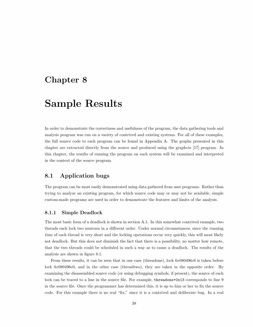
Chapter 8
Sample Results
In order to demonstrate the correctness and usefulness of the program, the data gathering tools and
analysis program was run on a variety of contrived and existing systems. For all of these examples,
the full source code to each program can be found in Appendix A. The graphs presented in this
chapter are extracted directly from the source and produced using the graphviz [17] program. In
this chapter, the results of running the program on each system will be examined and interpreted
in the context of the source program.
8.1 Application bugs
The program can be most easily demonstrated using data gathered from user programs. Rather than
trying to analyze an existing program, for which source code may or may not be available, simple
custom-made programs are used in order to demonstrate the features and limits of the analysis.
8.1.1 Simple Deadlock
The most basic form of a deadlock is shown in section A.1. In this somewhat contrived example, two
threads each lock two mutexes in a different order. Under normal circumstances, since the running
time of each thread is very short and the locking operations occur very quickly, this will most likely
not deadlock. But this does not diminish the fact that there is a possibility, no matter how remote,
that the two threads could be scheduled in such a way as to cause a deadlock. The results of the
analysis are shown in figure 8.1.
From these results, it can be seen that in one case (threadone), lock 0x080496c8 is taken before
lock 0x080496e0, and in the other case (threadtwo), they are taken in the opposite order. By
examining the disassembled source code (or using debugging symbols, if present), the source of each
lock can be traced to a line in the source file. For example, threadone+0x13 corresponds to line 9
in the source file. Once the programmer has determined this, it is up to him or her to fix the source
code. For this example there is no real “fix,” since it is a contrived and deliberate bug. In a real
38

39
080496e0
080496c8
Total Vertices: 2Total Edges: 2
Cycle found:080496c8:0 -> 080496e0:0
‘liblockgrab.so‘pthread_mutex_lock ‘liblockgrab.so‘pthread_mutex_lockthreadone+0x13 threadone+0x200x40032fa5 0x40032fa5‘libc.so.6‘__clone ‘libc.so.6‘__clone
080496e0:0 -> 080496c8:0
‘liblockgrab.so‘pthread_mutex_lock ‘liblockgrab.so‘pthread_mutex_lockthreadtwo+0x13 threadtwo+0x200x40032fa5 0x40032fa5‘libc.so.6‘__clone ‘libc.so.6‘__clone
Figure 8.1: Results of tracing a simple user deadlock
system there would be a more complex solution to the problem.
8.1.2 Dynamic Memory
The source code in section A.4 demonstrates the effect that dynamic memory allocation has on the
construction of the graph and subsequent analysis. We allocate lock a dynamically, and lock a and
then b. Then, we free and allocate the same lock (making sure that the address is the same), and
lock b and then a. Without generation counts, they would be treated as the same lock (since they
share the same address), and there would be a possible deadlock (as in figure 8.1). Instead, this
produces the set of events and resulting graph shown in figure 8.2.
These events are extracted from the original data and displayed in a human-readable format.
Note that the majority of the events are symbol declaration (SYM) events. For a complete description
of each event type, and the meaning of each parameter, consult section 6.2. The important event in
this data set is the generation count (GEN) event. This causes the generation count of 08049a10 to
be incremented to 1. In the graph, this creates a new node, and the resulting dependency does not
create a cycle.

40
SYM 4001774e ‘liblockgrab.so‘pthread mutex lockSYM 0804859b main+0x3bSYM 4005a0bf ‘libc.so.6‘ libc start mainSYM 080484a1 ‘test2‘pthread mutex unlockBLK 00000400 08049a10SYM 080485a7 main+0x47BLK 00000400 bffff744SYM 400179af ‘liblockgrab.so‘pthread mutex unlockSYM 080485b3 main+0x53REL 00000400 08049a10GEN 08049a10 08049a28SYM 080485fc main+0x9cBLK 00000400 08049a10SYM 08048608 main+0xa8REL 00000400 08049a10SYM 08048611 main+0xb1REL 00000400 bffff744
08049a10
bffff744
08049a10:1
Figure 8.2: Example of dynamic memory usage
8.1.3 The Dining Philosophers
One of the classic problems mentioned when discussing concurrency control is that of the dining
philosophers. In this problem, there are a number (N) of seats at a table with a place setting at
each seat. There is a fork on either side of the place setting, but the forks are shared between
adjacent place settings, so there are only N forks on the table. There are also N philosophers that
want to come and eat at the table. In order to eat at the table, the philosophers must grab both the
left fork and the right fork of a particular place setting. They cannot reach across the table, and
must wait until they have both forks before they can start eating. Once they pick up a fork, they
cannot put it down until they are done eating. The simplest solution is to have all the philosophers
sit down at the table, and grab the left fork and then the right fork. This is system in section A.2.
There is the possibility of a deadlock, however, if every philosopher picks up the left fork, at which
point no one can pick up their right fork or put down their left fork, and the entire table is in a
deadlock. The output from the program when it reaches the deadlock state with 3 philosophers is
shown in figure 8.3.
As the number of philosophers increase, and the amount of time spent eating decreases, the
chances of a deadlock being produced drop significantly. The analysis program should still be able
to detect the possibility of the deadlock, even if it isn’t produced during the execution of the program.
The results of the analysis are shown in figures 8.4 and 8.5 respectively. This analysis was performed
on a dining philosopher problem with 4 philosophers. One of the possible resolutions to this deadlock
problem is explained in the next section.

41
Running with 3 philosophersPhilosopher 1 waiting for left forkPhilosopher 1 left fork upPhilosopher 0 waiting for left forkPhilosopher 0 left fork upPhilosopher 2 waiting for left forkPhilosopher 2 left fork upPhilosopher 1 waiting for right forkPhilosopher 0 waiting for right forkPhilosopher 2 waiting for right fork
Figure 8.3: Dining philosophers in a deadlock
0804a1b0
0804a198
0804a1c8
0804a180
Figure 8.4: Graph of Dining philosophers
8.1.4 Dining Philosophers With a Butler
One of the possible solutions to the deadlock problem with the dining philosophers is the use of
a butler that effectively limits the number of people that can sit at the table. As long as there
are fewer philosophers at the table than there are place settings, the system cannot deadlock. The
source code for this example is given in section A.3. The difference between this example and the
previous dining philosopher solution is that the philosophers will pick up either fork first (a fact that
does not avoid the deadlock), as well as having the number sitting at the table limited to one less
than the total number of philosophers.
This example illustrates some of the shortcomings of the prediction mechanism. First of all,
it will predict the possibility of a deadlock between all of the philosophers, even though it cannot
actually occur. This is because it is impossible for the analysis program to know that there is an
overarching locking order that limits the number of threads that can be involved in the deadlock.
The deadlock is still reported due to the concurrency assumptions made about the system. Similarly,
the analysis will report a potential deadlock between each of the threads and itself, since in one case
it grabs the left fork and then the right fork, while in another instance it grabs the right fork and
then the left fork. This cannot actually occur in practice because there can only be one copy of each

42
Total Vertices: 4Total Edges: 4
Cycle found:0804a198:0 -> 0804a1b0:0
‘liblockgrab.so‘pthread_mutex_lock ‘liblockgrab.so‘pthread_mutex_lockphilosopher+0x84 philosopher+0xf90x40032fa5 0x40032fa5‘libc.so.6‘__clone ‘libc.so.6‘__clone
0804a180:0 -> 0804a198:0
‘liblockgrab.so‘pthread_mutex_lock ‘liblockgrab.so‘pthread_mutex_lockphilosopher+0x84 philosopher+0xf90x40032fa5 0x40032fa5‘libc.so.6‘__clone ‘libc.so.6‘__clone
0804a1c8:0 -> 0804a180:0
‘liblockgrab.so‘pthread_mutex_lock ‘liblockgrab.so‘pthread_mutex_lockphilosopher+0x84 philosopher+0xf90x40032fa5 0x40032fa5‘libc.so.6‘__clone ‘libc.so.6‘__clone
0804a1b0:0 -> 0804a1c8:0
‘liblockgrab.so‘pthread_mutex_lock ‘liblockgrab.so‘pthread_mutex_lockphilosopher+0x84 philosopher+0xf90x40032fa5 0x40032fa5‘libc.so.6‘__clone ‘libc.so.6‘__clone
Figure 8.5: Analysis of dining philosopher
philosopher thread running at any given time, but one of the concurrency assumptions was that it is
possible to have multiple copies of the same thread running at the same time. The existence of these
smaller cycles also shows the limitation of the cycle detection algorithm, because the smaller cycles
are not detected once the larger cycle is found. The results of the graph and the analysis are shown
in figures 8.6 and 8.7 respectively. Note that only one of the possible smaller cycles is detected.
8.2 Kernel Bugs
Part of the inspiration for this program was to provide a method of predicting deadlocks within an
operating system kernel. Two kernels were examined, the Linux kernel and the Solaris kernel, to
determine if either had an appropriate means of extracting lock data from a running system. The
Linux kernel has the beginnings of dynamic tracing facilities (see section 6.4) but they are not quite

43
080493e8
080493d0
08049400
bffff744
08049418
Figure 8.6: Graph of dining philosophers with a butler
adequate, and a full implementation would still be a reasonably large task. On the other hand, a
specially instrumented Solaris kernel was provided by the Solaris Kernel Group at Sun Microsystems,
providing a simple method of extracting data from an executing kernel. Therefore, all of the kernel
analysis is performed on the Solaris kernel, for the sake of simplicity.
Since the Solaris kernel has been around for a long time (and is one of the earliest fully preemptive
UNIX kernels), it has undergone a rigorous test regimen during its evolution. It is highly unlikely
that there are any existing bugs in the common kernel code. It is much more likely that deadlocks
exist in some of the newer and more esoteric modules that are not used very often. Without access
to some of the newest hardware and modules, a special kernel driver was instead created in order
to artificially insert deadlocks into the kernel. The complete source code for this driver is given in
sections A.5 and A.6. This driver was then installed in the system as /dev/badlock, and tested
with the code in section A.7. The device allows for several different tests through the ioctl() call,
the specifics of each which is discussed here.
8.2.1 Locking Order
This test (BADLOCK CHECK ORDER) is the kernel version of the test described in section 8.1.1. It merely
locks two different locks in two different orders, using the kernel-level functions mutex enter and
mutex exit. If two different user programs were to issue this ioctl at precisely the right moment,
it would be possible that they would both deadlock, and the rest of the driver becomes unusable (a
bigger problem with realistic systems). The results of the analysis on this section of the driver is
shown in figure 8.8.
Note that in this particular test, the mutexes are actually on the stack, so it is impossible for any
two threads to ever deadlock on these mutexes. This makes the code simpler, although the analysis
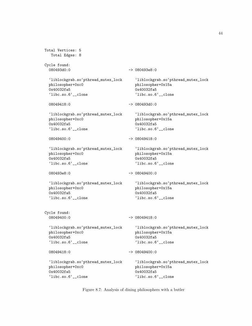
44
Total Vertices: 5Total Edges: 8
Cycle found:080493d0:0 -> 080493e8:0
‘liblockgrab.so‘pthread_mutex_lock ‘liblockgrab.so‘pthread_mutex_lockphilosopher+0xc0 philosopher+0x15a0x40032fa5 0x40032fa5‘libc.so.6‘__clone ‘libc.so.6‘__clone
08049418:0 -> 080493d0:0
‘liblockgrab.so‘pthread_mutex_lock ‘liblockgrab.so‘pthread_mutex_lockphilosopher+0xc0 philosopher+0x15a0x40032fa5 0x40032fa5‘libc.so.6‘__clone ‘libc.so.6‘__clone
08049400:0 -> 08049418:0
‘liblockgrab.so‘pthread_mutex_lock ‘liblockgrab.so‘pthread_mutex_lockphilosopher+0xc0 philosopher+0x15a0x40032fa5 0x40032fa5‘libc.so.6‘__clone ‘libc.so.6‘__clone
080493e8:0 -> 08049400:0
‘liblockgrab.so‘pthread_mutex_lock ‘liblockgrab.so‘pthread_mutex_lockphilosopher+0xc0 philosopher+0x15a0x40032fa5 0x40032fa5‘libc.so.6‘__clone ‘libc.so.6‘__clone
Cycle found:08049400:0 -> 08049418:0
‘liblockgrab.so‘pthread_mutex_lock ‘liblockgrab.so‘pthread_mutex_lockphilosopher+0xc0 philosopher+0x15a0x40032fa5 0x40032fa5‘libc.so.6‘__clone ‘libc.so.6‘__clone
08049418:0 -> 08049400:0
‘liblockgrab.so‘pthread_mutex_lock ‘liblockgrab.so‘pthread_mutex_lockphilosopher+0xc0 philosopher+0x15a0x40032fa5 0x40032fa5‘libc.so.6‘__clone ‘libc.so.6‘__clone
Figure 8.7: Analysis of dining philosophers with a butler

45
Cycle found:000002a100571968:0 -> 000002a100571970:0
unix‘mutex_enter unix‘mutex_enterbadlock‘badlockdrv_ioctl+0x7c badlock‘badlockdrv_ioctl+0x8cgenunix‘ioctl+0x1f8 genunix‘ioctl+0x1f8
000002a100571970:0 -> 000002a100571968:0
unix‘mutex_enter unix‘mutex_enterbadlock‘badlockdrv_ioctl+0x74 badlock‘badlockdrv_ioctl+0x7cgenunix‘ioctl+0x1f8 genunix‘ioctl+0x1f8
Figure 8.8: Kernel locking order deadlock
is technically incorrect. In reality, it makes little sense to have mutexes on the stack, and these
would more likely be allocated from some shared memory (or declared statically) so that they could
be shared between threads. Note also that in the results the addresses are 64 bits (since the kernel is
a sun4u 64-bit kernel), demonstrating the ability to deal with different sizes for the primitive types.
8.2.2 Dynamic Memory
This call (BADLOCK CHECK FREE) is the kernel-level equivalent of the example shown in section 8.1.2.
It allocates a mutex a from a cache using kmem cache alloc, locks a and then another static mutex
b. The dynamic mutex is freed using kmem cache free and then allocated again, returning the
same address. The locks are then locked in the reverse order, but since the new a is logically a
different lock (even though is shares the same address) it is not a deadlock. Running the analysis
tools doesn’t show any deadlock in this section of code, demonstrating that the dynamic allocation
is correctly handled. Unfortunately, the number of events (and the resulting graph) are so large that
they cannot be shown here in order to prove that the cycle doesn’t exist in the graph.
8.2.3 Recursive Reader-Writer Lock
As described in section 5.2, the problem of recursive read locks on a reader-writer lock is a relatively
common problem in large systems. This test (BADLOCK CHECK RWLOCK) takes two consecutive read
lock using rw enter(&lock, RW READER). Under normal circumstances, the second call will almost
never block, since it would require an intervening write call to occur at just the precise moment
between the two locking attempts. There is this slight chance, leading to the possibility of a deadlock.
The results of running the analysis is shown in figure 8.9.
Note that the cycle is detected between the lock and itself. This is the only situation where this
can occur in normal locking systems, except for the case of semaphores. Otherwise, the second call to
the acquisition function would have blocked, and the system would have deadlocked instantly. Again,
in this contrived situation, the locks are located on the stack, and there is no way for an intervening

46
Cycle found:000002a100571958:0 -> 000002a100571958:0
unix‘rw_enter unix‘rw_enterbadlock‘badlockdrv_ioctl+0x1fc badlock‘badlockdrv_ioctl+0x208genunix‘ioctl+0x1f8 genunix‘ioctl+0x1f8
Figure 8.9: Recursive reader-writer locks in the kernel
write attempt to happen, so there is technically no possibility of a deadlock. In a real situation,
these locks would be shared by threads, and there is an implicit assumption that somewhere, a write
lock will be taken.
8.2.4 Interrupt Dependent Functions
This type of locking violation is described in section 5.4. As outlined there, the kmem alloc function
requires interrupts of level 7 to be able to complete when passed the KM SLEEP flag. This is because in
low memory situations, the pageout daemon needs to run, which requires the I/O completion routines
need to run at interrupt level 7. In order to test the functionality of this detection, the driver takes
a lock (thread free lock) that is known to be taken in the clock handler. The current process
p lock could have been used as well, but it doesn’t matter, since the dependency is automatically
detected. Once this lock is acquired, kmem alloc is called with the KM SLEEP flag. The original lock
is then released. The results of the analysis are shown in figure 8.10.
Cycle found:0000000000000009:0 -> 000000000000000a:00000000000000008:0 -> 0000000000000009:00000000000000007:0 -> 0000000000000008:00000000001899720:0 -> 0000000000000007:0
unix‘mutex_enter genunix‘kmem_cache_allocbadlock‘badlockdrv_ioctl+0x24c genunix‘kmem_alloc+0x28genunix‘ioctl+0x1f8 badlock‘badlockdrv_ioctl+0x258
genunix‘ioctl+0x1f8
000000000000000a:0 -> 0000000001899720:0
unix‘mutex_entergenunix‘clock+0x36cgenunix‘cyclic_softint+0x368unix‘cbe_level10+0x8
Figure 8.10: Interrupt Dependent Functions in the Kernel
The pseudo-locks for each interrupt are represented as their numerical identity. This is safe
because in the Solaris kernel we are assured that there is no memory mapped in the first page of

47
memory, so these pseudo-locks will never conflict with the address of any real lock. The implicit
dependencies are shown between each interrupt level (notice that there are no events associated with
the implicit dependencies). The clock interrupt occurs at level 10, but the implicit dependencies
connect this to the dependency created at level 7 by the driver. In the future, the program could
be modified so that locks can have symbolic names attached to them, so that the interrupts would
appear as “IPL 9”, “IPL 10”, etc, and the lock itself could appear as “thread free lock” (since it is
statically defined).
8.3 Existing Solaris Bugs
Despite the claims made at the beginning of this chapter, some potential deadlocks still exist in the
Solaris kernel, and a few were found using this tool. Most notably, two potential deadlocks were
found in the UFS (Unix File System) subsystem.
While it may seem that deadlocks in such a common subsystem should have been long since
fixed, the deadlocks are in fact extremely unlikely to occur, since they rely on several infrequently
used features of UFS. UFS supports quotas, allowing filesystems to be limited in their size, as well
as access control lists (ACLs) and attribute directories. To begin with, both deadlocks involve a
global reader-writer lock designed to prevent simultaneous access to quota data. The quota data
is accessed by acquiring a read lock whenever a file is added or deleted. Normally, when a file is
deleted, a read lock on the quota is taken (to prevent it from changing value) and the file is removed
from the system. If the directory contains ACLs or an attribute directory, then a recursive read lock
ends up being taken. The code to remove the file from the directory gets a read lock on the global
lock, but then calls another subroutine with it held, and that subroutine ends up taking the same
lock again. Normally, this function is called from routines that do not already have the lock. The
only time a write lock is taken on the global lock is via the quotacheck and edquota commands,
so if one of these commands is run at just the right time and the write lock occurs between the two
read locks, while an ACL or attribute directory is being deleted, then the entire UFS subsystem will
deadlock.
It is apparent that this is a highly unlikely bug, since it requires that the administrator have
access control lists and/or attribute directories, and that a certain command be run at precisely the
same time that a file is being deleted. Nevertheless, it is a potential deadlock, and any such situation
is a hurdle to achieving the elusive goal of 100% uptime. In order to find this bug, a UFS stress test
was run while data was gathered from the entire kernel. In order to keep the file sizes manageable,
data was gathered into 2 or 3 minute groups, where each file was about one to two gigabytes long
(see section 8.4). Each of these files was then analyzed independently, and these cycles were detected
in the graph. From looking at the stack traces, it was apparent that the subroutine was being called
with the same lock held. From this point, it was a relatively simple matter to trace through the
source code to determine exactly how it got there.

48
8.4 Kernel Complexity
Some passing references have been made to the complexity of analyzing locks in a preemptive kernel.
To shed some light on the subject, a few arbitrary tests were done in order to gather basic statistics
about the number of locks to expect in a typical trace of the Solaris kernel. To begin with, a simple
trace of all the mutex operations (not including spin locks) when running the “date” command
was done. From the kernel view, this command simply maps some memory, makes a system call
to find out the current time, and then makes another system call to write to the screen device.
To acquire this data, operations were only recorded if curthread->t procp->p user->u comm was
equal to “date”. Running the command once produced 9000 events, and the resulting graph had
500 vertices and 14,000 edges. This is one of the simplest traces possible and already the graphviz
program requires 180 pages to display the resulting graph.
For a more general situation, a trace of the entire kernel (without spin locks) on an “idle” system
(one in which the majority of processes are blocked waiting for I/O and not actively consuming
system resources) yields more realistic results. In a 5 second trace, a graph with 3700 locks and
27000 edges is produced. A minute of tracing an idle system produces approximately half a gigabyte
of data, or 1 million records. More moderately loaded systems, when including spin locks, generate
about 10 million records per minute, and the resulting graphs can have upwards of 25,000 vertices
and 250,000 edges. Since a typical coverage test can be expected to run for times ranging from 5
minutes to an hour for complicated systems, we can expect to see traces with hundreds of millions
of events and millions of dependencies. At this point, the current implementation starts to reach
the limits of the hardware available to the author. Significant work can still go into optimizing the
source code (the first step being to turn debugging information off), and more powerful hardware
(including multiprocessor machines) can be used to construct more comprehensive analyses.

Chapter 9
Concluding Remarks
Deadlock detection and prediction is not a new idea, and has been around since multiprogramming
was first introduced. The problem of deadlock prediction is an especially important one, since
most systems need to be deadlock-free. This problem is unfortunately also a very difficult one.
Throughout the course of this thesis, a practical and extensible solution to this problem has been
presented.
The main benefit of this system is that it allows for prediction and modeling of systems that
were previously inaccessible. Large concurrent systems can be easily analyzed for possible deadlocks,
including operating system kernels. The separation of the analysis and data gathering tools allow
for data to be extracted from a variety of systems and all analyzed using the same program, making
it easy to expand the analysis to novel systems. In addition, a variety of other synchronization tools
can be modeled effectively, including interrupt handlers and non-blocking locks. With the automatic
handling of dynamic memory, this system can effectively model situations that historically have been
unassailable.
Using a dynamic tracing framework, data can be directly extracted from sources, without re-
quiring the programmer to change any code or recompile any software. This trace-driven technique
also allows for data to be extracted from an executing kernel, which makes kernel analysis possible.
This reduces the overhead at run time, instead opting to stream the data to an external source for
later analysis.
The analysis of the system is not perfect, since it relies on several assumptions about the con-
current nature of the system that may not always hold true. Some deadlocks may be reported that
can in fact never occur, since there are constraints on the system beyond the traditional model, or
violations of the concurrency assumptions. Once these deadlocks are reported, then, it becomes the
responsibility of the programmer to return to the source code and determine if the deadlock in fact
exists, and what can be done to fix it.
The overall system demonstrates that it is possible to predict deadlocks in a complicated system
such as an operating system, without impacting the run time performance. A great deal more
work can be done into making the interface more accessible, with the possibility of integrating the
49

50
analysis into a coherent development tool. The algorithms used could also be optimized or extended,
though the basic concepts are sound. The largest area where this research can be extended is
applying to new and novel systems, such as the Linux kernel or distributed systems. As long as
the concurrency constraints follow the assumptions laid out, and the concurrency controls follow
traditional semantics, then any system can be targeted.
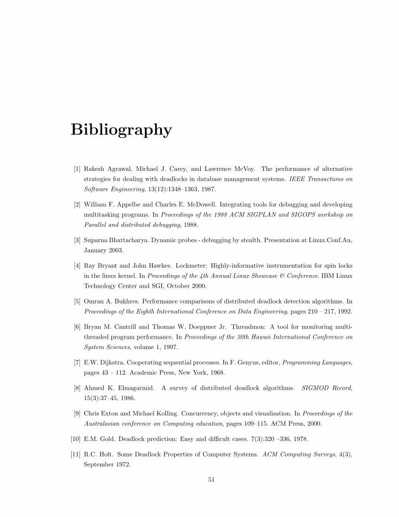
Bibliography
[1] Rakesh Agrawal, Michael J. Carey, and Lawrence McVoy. The performance of alternative
strategies for dealing with deadlocks in database management systems. IEEE Transactions on
Software Engineering, 13(12):1348–1363, 1987.
[2] William F. Appelbe and Charles E. McDowell. Integrating tools for debugging and developing
multitasking programs. In Proceedings of the 1988 ACM SIGPLAN and SIGOPS workshop on
Parallel and distributed debugging, 1988.
[3] Suparna Bhattacharya. Dynamic probes - debugging by stealth. Presentation at Linux.Conf.Au,
January 2003.
[4] Ray Bryant and John Hawkes. Lockmeter: Highly-informative instrumentation for spin locks
in the linux kernel. In Proceedings of the 4th Annual Linux Showcase & Conference. IBM Linux
Technology Center and SGI, October 2000.
[5] Omran A. Bukhres. Performance comparisons of distributed deadlock detection algorithms. In
Proceedings of the Eighth International Conference on Data Engineering, pages 210 – 217, 1992.
[6] Bryan M. Cantrill and Thomas W. Doeppner Jr. Threadmon: A tool for monitoring multi-
threaded program performance. In Proceedings of the 30th Hawaii International Conference on
System Sciences, volume 1, 1997.
[7] E.W. Dijkstra. Cooperating sequential processes. In F. Genyus, editor, Programming Languages,
pages 43 – 112. Academic Press, New York, 1968.
[8] Ahmed K. Elmagarmid. A survey of distributed deadlock algorithms. SIGMOD Record,
15(3):37–45, 1986.
[9] Chris Exton and Michael Kolling. Concurrency, objects and visualisation. In Proceedings of the
Australasian conference on Computing education, pages 109–115. ACM Press, 2000.
[10] E.M. Gold. Deadlock prediction: Easy and difficult cases. 7(3):320 –336, 1978.
[11] R.C. Holt. Some Deadlock Properties of Computer Systems. ACM Computing Surveys, 4(3),
September 1972.
51

52
[12] Institute of Electrical and Electronic Engineers, Inc. Information Technology – Portable Op-
erating System Interface (POSIX). IEEE Standard 1003.1-2001, IEEE, New York City, New
York, USA, 2001. also Single UNIX Specification.
[13] Kai Software. Tutorial: Using Assure for Threads, 2001.
[14] David B. Lomet. A practical deadlock avoidance algorithm for data base systems. In Proceedings
of the 1977 ACM SIGMOD international conference on Management of data. IBM Thomas J.
Watson Research Center, 1977.
[15] D. Menasce and R. Muntz. Locking and deadlock detection in distributed data bases. IEEE
Transactions on Software Engineering, 5(3), May 1979.
[16] Richard Moore. A universal dynamic trace for linux and other operating systems. In Proceedings
of the USENIX Annual Technical Conference. IBM Linux Technology Center, June 2001.
[17] AT&T Labs Research. Graphviz - open source drawing software.
http://www.research.att.com/sw/tools/graphviz/.
[18] M. Roesler and W. A. Burkhard. Semantic lock models in object-oriented distributed systems
and deadlock resolution. In Proceedings of the 1988 ACM SIGMOD international conference
on Management of data, pages 361–370. ACM Press, 1988.
[19] SGI. Kernprof - linux kernel profiling. http://oss.sgi.com/projects/kernprof.
[20] Stephen W. Sherman. Trace driven modeling: An update. In Proceedings of the fourth sympo-
sium on Simulation of computer systems, pages 87–91, 1976.
[21] Pun Hang Shiu, Yudong Tan, and Vincent John Mooney III. A novel parallel deadlock de-
tection algorithm and architecture. In Proceedings of the ninth international symposium on
Hardware/software codesign, pages 73–78, 2001.
[22] Kai Software. Assure thread analyzer. http://developer.intel.com/software/products/assure/.
[23] Sun Microsystems, Inc. Multithreaded Programming Guide, 1997. Solaris 7 Software Developer
Collection.
[24] Sun Microsystems, Inc. Programming Utilities Guide, 1997. Solaris 7 Software Developer
Collection.
[25] Sun Microsystems, Inc. lockstat(1M) manual page, 2001. Solaris 8 Reference Manual Collection.
[26] Ariel Tamches. Fine-Grained Dynamic Instrumentation of Commodity Operating System Ker-
nels. PhD thesis, University of Wisconsin, Madison, Wisconsin, February 2001.
[27] Ariel Tamches and Barton P. Miller. Using dynamic kernel instrumentation for kernel and
application tuning. International Journal of High-Performance and Applications, 13(3), Fall
1999.

53
[28] Andrew S. Tanenbaum. Modern Operating Systems. Prentice Hall, 2nd edition, 2001.
[29] Richard N. Taylor. Complexity of analyzing the synchronization structure of concurrent pro-
grams. Acta Informatica, 19:57 – 84, 1983.
[30] Richard N. Taylor. A general-purpose algorithm for analyzing concurrent programs. CACM,
26(5):362 – 376, May 1983.
[31] Richard N. Taylor. Debugging real-time software in a host-target environment. Technical Report
212, U.C. Irvine, 1984.
[32] Henry Tirri. Freedom from deadlock of locked transactions in a distributed database. In
Proceedings of the second annual ACM symposium on Principles of distributed computing, pages
267–276, 1983.
[33] Karim Yaghmour and Michel R. Dagenais. Measuring and characterizing system behavior
using kenrel-level event logging. In USENIX Annual Technical Conference Proceedings. Ecole
Polytechnique de Montreal, June 2000.
[34] Michal Young, Richard N. Taylor, Kari Forester, and Debra Brodbeck. Integrated concurrency
analysis in a software development environment. In Proceedings of the ACM SIGSOFT ’89
Third Symposium on Software Testing, Analysis and Verifcation, pages 200 – 209, December
1989.
Appendix A
Source Code Examples
A.1 Simple User Deadlock
#include <pthread.h>#include <assert.h>
static pthread_mutex_t a = PTHREAD_MUTEX_INITIALIZER;static pthread_mutex_t b = PTHREAD_MUTEX_INITIALIZER;
static void * threadone(void *param){
pthread_mutex_lock(&a);pthread_mutex_lock(&b);pthread_mutex_unlock(&b);pthread_mutex_unlock(&a);
}
static void * threadtwo(void *param){
pthread_mutex_lock(&b);pthread_mutex_lock(&a);pthread_mutex_unlock(&a);pthread_mutex_unlock(&b);
}
int main(int argc, char **argv){
int ret;pthread_t t1, t2;
ret = pthread_create(&t1, NULL, threadone, NULL);assert(ret == 0);ret = pthread_create(&t2, NULL, threadtwo, NULL);assert(ret == 0);
54

55
pthread_join(t1, NULL);pthread_join(t2, NULL);return 0;
}
A.2 Dining Philosophers
#include <pthread.h>#include <stdio.h>#include <unistd.h>#include <stdlib.h>#include <signal.h>#include <assert.h>#include <time.h>
typedef struct placesetting {pthread_mutex_t *forks[2];int number;
} placesetting_t;
static int g_stopped;
void *philosopher(void *param){
placesetting_t *place = (placesetting_t *)param;struct timespec delay;
delay.tv_sec = 0;
while (!g_stopped) {/* Wait for up to 100 ms */delay.tv_nsec = rand() % 100000000;nanosleep(&delay, NULL);
/* Get left fork */printf("Philosopher %d waiting for left fork\n",
place->number );pthread_mutex_lock(place->forks[0]);printf("Philosopher %d left fork up\n",
place->number);
/* Wait for up to 100 ms */delay.tv_nsec = rand() % 100000000;nanosleep(&delay, NULL);
/* Get right fork */printf("Philosopher %d waiting for right fork\n",
place->number);pthread_mutex_lock(place->forks[1]);
56
printf("Philosopher %d right fork up\n",place->number);
/* Wait for up to 100 ms */delay.tv_nsec = rand() % 100000000;nanosleep(&delay, NULL);
/* Release forks */printf("Philosopher %d right fork down\n",
place->number);pthread_mutex_unlock(place->forks[1]);printf("Philosopher %d left fork down\n",
place->number);pthread_mutex_unlock(place->forks[0]);
}}
intmain(int argc, char **argv){
int count;pthread_mutex_t *forks;placesetting_t *places;pthread_t *philosophers;int i;int ret, sig;sigset_t set;
if (argc != 2) {printf("usage: %s count\n", argv[0]);return EXIT_FAILURE;
}
count = atoi(argv[1]);if (count <= 1) {
printf("usage: %s count\n", argv[0]);return EXIT_FAILURE;
}
printf("Running with %d philosophers\n", count);srand(time(NULL));
/* Create the placesettings */forks = malloc(count * sizeof(pthread_mutex_t));places = malloc(count * sizeof(placesetting_t));philosophers = malloc(count * sizeof(pthread_t));
for (i = 0; i < count; i++) {pthread_mutex_init(&forks[i], NULL);places[i].number = i;places[i].forks[0] = &forks[i];

57
places[i].forks[1] = &forks[(i+1)%count];}
/* Create the philosopher threads */sigemptyset(&set);sigaddset(&set, SIGINT);pthread_sigmask(SIG_BLOCK, &set, 0);
for (i = 0; i < count; i++) {ret = pthread_create(&philosophers[i], NULL, philosopher,
&places[i]);assert(ret == 0);
}
sigwait(&set, &sig);/* This is not technically thread-safe, but it will do */g_stopped = 1;
for (i = 0; i < count; i++) {ret = pthread_join(philosophers[i], NULL);assert(ret == 0);
}
return EXIT_SUCCESS;}
A.3 Dining Philosophers With a Butler
#include <pthread.h>#include <stdio.h>#include <unistd.h>#include <stdlib.h>#include <signal.h>#include <assert.h>#include <time.h>
typedef struct butler {pthread_mutex_t mtx;pthread_cond_t cond;int count;
} butler_t;
typedef struct placesetting {pthread_mutex_t *forks[2];int number;butler_t *butler;
} placesetting_t;
static int g_stopped;

58
static voidbutler_init(butler_t *b, int count){
pthread_mutex_init(&b->mtx, NULL);pthread_cond_init(&b->cond, NULL);b->count = count;
}
static voidbutler_enter(butler_t *b){
pthread_mutex_lock(&b->mtx);while(b->count == 0)
pthread_cond_wait(&b->cond, &b->mtx);b->count--;pthread_mutex_unlock(&b->mtx);
}
static voidbutler_leave(butler_t *b){
pthread_mutex_lock(&b->mtx);b->count++;pthread_cond_broadcast(&b->cond);pthread_mutex_unlock(&b->mtx);
}
void *philosopher(void *param){
static char * fork_names[2] = { "left", "right" };placesetting_t *place = (placesetting_t *)param;struct timespec delay;int first;
delay.tv_sec = 0;
while (!g_stopped) {/* Request permission from the butler */butler_enter(place->butler);
/* Randomly pick which fork to choose */first = rand() & 1;
/* Wait for up to 100 ms */delay.tv_nsec = rand() % 100000000;nanosleep(&delay, NULL);
/* Get first fork */printf("Philosopher %d waiting for %s fork\n",
place->number, fork_names[first]);

59
pthread_mutex_lock(place->forks[first]);printf("Philosopher %d %s fork up\n",
place->number, fork_names[first]);
first = !first;
/* Wait for up to 100 ms */delay.tv_nsec = rand() % 100000000;nanosleep(&delay, NULL);
/* Get second fork */printf("Philosopher %d waiting for %s fork\n",
place->number, fork_names[first]);pthread_mutex_lock(place->forks[first]);printf("Philosopher %d %s fork up\n",
place->number, fork_names[first]);
/* Wait for up to 100 ms */delay.tv_nsec = rand() % 100000000;nanosleep(&delay, NULL);
/* Release forks */printf("Philosopher %d %s fork down\n",
place->number, fork_names[first]);pthread_mutex_unlock(place->forks[first]);first = !first;printf("Philosopher %d %s fork down\n",
place->number, fork_names[first]);pthread_mutex_unlock(place->forks[first]);
/* Tell the butler we’re leaving */butler_leave(place->butler);
}}
intmain(int argc, char **argv){
int count;pthread_mutex_t *forks;placesetting_t *places;pthread_t *philosophers;int i;int ret, sig;sigset_t set;butler_t butler;
if (argc != 2) {printf("usage: %s count\n", argv[0]);return EXIT_FAILURE;
}

60
count = atoi(argv[1]);if (count <= 1) {
printf("usage: %s count\n", argv[0]);return EXIT_FAILURE;
}
printf("Running with %d philosophers\n", count);srand(time(NULL));
/* Initialize the butler */butler_init(&butler, count-1);
/* Create the placesettings */forks = malloc(count * sizeof(pthread_mutex_t));places = malloc(count * sizeof(placesetting_t));philosophers = malloc(count * sizeof(pthread_t));
for (i = 0; i < count; i++) {pthread_mutex_init(&forks[i], NULL);places[i].number = i+1;places[i].forks[0] = &forks[i];places[i].forks[1] = &forks[(i+1)%count];places[i].butler = &butler;
}
/* Create the philosopher threads */sigemptyset(&set);sigaddset(&set, SIGINT);pthread_sigmask(SIG_BLOCK, &set, 0);
for (i = 0; i < count; i++) {ret = pthread_create(&philosophers[i], NULL, philosopher,
&places[i]);assert(ret == 0);
}
sigwait(&set, &sig);/* This is not technically thread-safe, but it will do */g_stopped = 1;
for (i = 0; i < count; i++) {ret = pthread_join(philosophers[i], NULL);assert(ret == 0);
}
return EXIT_SUCCESS;}

61
A.4 Dynamic Memory
#include <assert.h>#include <stdio.h>#include <stdlib.h>#include <pthread.h>
intmain(){
pthread_mutex_t *a, b = PTHREAD_MUTEX_INITIALIZER, *save;
save = a = malloc(sizeof(pthread_mutex_t));pthread_mutex_init(a, NULL);pthread_mutex_lock(a);pthread_mutex_lock(&b);pthread_mutex_unlock(a);free(a);a = malloc(sizeof(pthread_mutex_t));assert(a == save);pthread_mutex_init(a, NULL);pthread_mutex_lock(a);pthread_mutex_unlock(a);pthread_mutex_unlock(&b);
return (0);}
A.5 Solaris Kernel Module
#include <sys/types.h>#include <sys/stat.h>#include <sys/modctl.h>#include <sys/cmn_err.h>#include <sys/errno.h>
#include <sys/systm.h>#include <sys/ddi.h>#include <sys/sunddi.h>#include <sys/devops.h>#include <sys/conf.h>
#include "badlock.h"
static dev_info_t *badlockdrv_devi;
static intbadlockdrv_open(dev_t *devp, int flag, int otyp, cred_t *cred_p){
return (0);

62
}
static intbadlockdrv_close(dev_t dev, int flag, int otyp, cred_t *cred_p){
return (DDI_SUCCESS);}
static intbadlockdrv_ioctl(dev_t dev, int cmd, intptr_t data, int flag, cred_t *cred,
int *rvalp){
switch(cmd) {
/** This checks the obvious case, where we acquire A then B in one case,* and later acquire B then A. This should be recognized as an error.*/case BADLOCK_CHECK_ORDER:{
kmutex_t a, b;
mutex_init(&a, NULL, MUTEX_DRIVER, NULL);mutex_init(&b, NULL, MUTEX_DRIVER, NULL);
mutex_enter(&a);mutex_enter(&b);mutex_exit(&a);mutex_enter(&a);mutex_exit(&a);mutex_exit(&b);
mutex_destroy(&a);mutex_destroy(&b);
}break;
/** This checks that memory that we free is not erroneously identified* as the same lock. This should NOT produce an error. What we are* going to do is:** allocate A from cache* lock X* lock A* unlock A* unlock X* return A to cache** allocate B from cache (same address)* lock B

63
* lock X* unlock X* unlock B* return B to cache** By address, this would be a locking violation. But by the fact that* it is freed, A and B should be considered different locks.*/case BADLOCK_CHECK_FREE:{
kmutex_t x;kmutex_t *a, *b;kmem_cache_t *mutex_cache;
mutex_init(&x, NULL, MUTEX_DRIVER, NULL);mutex_cache = kmem_cache_create("badlock_cache",
sizeof (kmutex_t), 0, NULL, NULL, NULL, NULL, NULL, 0);
a = kmem_cache_alloc(mutex_cache, KM_SLEEP);mutex_init(a, NULL, MUTEX_DRIVER, NULL);mutex_enter(&x);mutex_enter(a);mutex_exit(a);mutex_exit(&x);mutex_destroy(a);kmem_cache_free(mutex_cache, a);
b = kmem_cache_alloc(mutex_cache, KM_SLEEP);mutex_init(b, NULL, MUTEX_DRIVER, NULL);mutex_enter(b);mutex_enter(&x);mutex_exit(&x);mutex_exit(b);mutex_destroy(b);kmem_cache_free(mutex_cache, b);
kmem_cache_destroy(mutex_cache);mutex_destroy(&x);
/** We want to make sure that we did in fact allocate to the* same address. This should always be true, considering that* no one else if using this cache.*/
if (a != b)return (-1);
elsereturn (0);
}break;

64
/** This case checks that recursive read locks on rwlocks are correctly* identified. If a read lock is taken on a rwlock that is already* owned for reading, an intervening write lock could result in a* deadlock.*/case BADLOCK_CHECK_RWLOCK:{
krwlock_t lock;
rw_init(&lock, NULL, RW_DRIVER, NULL);rw_enter(&lock, RW_READER);rw_enter(&lock, RW_READER);rw_exit(&lock);rw_exit(&lock);rw_destroy(&lock);
}break;
/** This case checks that IPL-dependent functions are detected. Any* allocations with KM_SLEEP cannot be done with thread_free_lock held,* because it implicitly relies on I/O completion routines for* the pageout daemon, which require Interrupts at level 7 to be* serviceable. Since the clock routine runs at level 10 and requires* thread_free_lock, we have a potential deadlock.*/case BADLOCK_CHECK_PIL:{
void * mem;
mutex_enter(&thread_free_lock);
mem = kmem_alloc(1, KM_SLEEP);kmem_free(mem, 1);
mutex_exit(&thread_free_lock);}break;
default:return (-1);
}
return (0);}
static intbadlockdrv_info(dev_info_t *dip, ddi_info_cmd_t infocmd, void *arg, void **result){

65
int error;
switch (infocmd) {case DDI_INFO_DEVT2DEVINFO:
*result = (void *) badlockdrv_devi;error = DDI_SUCCESS;break;
case DDI_INFO_DEVT2INSTANCE:*result = (void *)0;error = DDI_SUCCESS;break;
default:error = DDI_FAILURE;
}return (error);
}
static intbadlockdrv_attach(dev_info_t *devi, ddi_attach_cmd_t cmd){
switch (cmd) {case DDI_ATTACH:
break;
case DDI_RESUME:return (DDI_SUCCESS);
default:return (DDI_FAILURE);
}
if (ddi_create_minor_node(devi, "badlock", S_IFCHR,0, DDI_PSEUDO, 0) == DDI_FAILURE) {
ddi_remove_minor_node(devi, NULL);return (DDI_FAILURE);
}
badlockdrv_devi = devi;
ddi_report_dev(devi);return (DDI_SUCCESS);
}
static intbadlockdrv_detach(dev_info_t *devi, ddi_detach_cmd_t cmd){
switch (cmd) {case DDI_DETACH:
break;
case DDI_SUSPEND:

66
return (DDI_SUCCESS);
default:return (DDI_FAILURE);
}
ddi_remove_minor_node(devi, NULL);return (DDI_SUCCESS);
}
/** Configuration data structures*/static struct cb_ops badlockdrv_cb_ops = {
badlockdrv_open, /* open */badlockdrv_close, /* close */nulldev, /* strategy */nulldev, /* print */nodev, /* dump */nodev, /* read */nodev, /* write */badlockdrv_ioctl, /* ioctl */nodev, /* devmap */nodev, /* mmap */nodev, /* segmap */nochpoll, /* poll */ddi_prop_op, /* cb_prop_op */0, /* streamtab */D_MP | D_NEW /* Driver compatibility flag */
};
static struct dev_ops badlockdrv_ops = {DEVO_REV, /* devo_rev, */0, /* refcnt */badlockdrv_info, /* getinfo */nulldev, /* identify */nulldev, /* probe */badlockdrv_attach, /* attach */badlockdrv_detach, /* detach */nulldev, /* reset */&badlockdrv_cb_ops, /* cb_ops */(struct bus_ops *)0, /* bus_ops */
};
static struct modldrv modldrv = {&mod_driverops, /* Type of module. This one is a driver */"Bad Lock Driver", /* name of module */&badlockdrv_ops, /* driver ops */
};
static struct modlinkage modlinkage = {

67
MODREV_1, (void *)&modldrv, NULL};
int_init(void){
return (mod_install(&modlinkage));}
int_fini(void){
return (mod_remove(&modlinkage));}
int_info(struct modinfo *modinfop){
return (mod_info(&modlinkage, modinfop));}
A.6 Solaris Kernel Module Header
#ifndef _BADLOCK_H#define _BADLOCK_H
#ifdef __cplusplusextern "C" {#endif
#define BADLOCK_CHECK_ORDER 1#define BADLOCK_CHECK_FREE 2#define BADLOCK_CHECK_RWLOCK 3#define BADLOCK_CHECK_PIL 4
#define BADLOCK_MIN 1#define BADLOCK_MAX 4
#ifdef __cplusplus}#endif
#endif /* _BADLOCK_H */
A.7 Solaris Kernel Driver
#include <stdio.h>#include <sys/ioctl.h>#include <stdlib.h>

68
#include <sys/types.h>#include <sys/stat.h>#include <fcntl.h>#include <unistd.h>
#include "badlock.h"
intmain(int argc, char **argv){
int fd;int i;
if ((fd = open("/dev/badlock", O_RDWR)) == -1) {fprintf(stderr, "Unable to open /dev/badlock\n");return (EXIT_FAILURE);
}
for (i = BADLOCK_MIN; i <= BADLOCK_MAX; i++) {if (ioctl(fd, i) < 0) {
fprintf(stderr, "ioctl() %d failed\n", i);return (EXIT_FAILURE);
}}
if (close(fd) < 0) {fprintf(stderr, "close() failed for /dev/badlock\n");return (EXIT_FAILURE);
}
return (EXIT_SUCCESS);}