dynamic load balancing of a power system portfoliojbjo/phd_thesis_2010_kristianedlund.pdfthis thesis...
TRANSCRIPT

Kristian Edlund
Dynamic Load Balancingof a Power System Portfolio

Dynamic Load Balancing of a Power System PortfolioPh.D. thesis
ISBN: 123-223-445April 2010
Copyright 2007-2010c© Kristian Edlund except where otherwise stated.
Contents
Contents III
Preface VII
Abstract IX
Synopsis XI
1 Introduction 11.1 Motivation . . . . . . . . . . . . . . . . . . . . . . . . . . . . . . . . . . 11.2 Power Systems Control and Electricity Market . . . . . . . . .. . . . . . 31.3 State of the Art and Background of Chosen Methodology . . .. . . . . . 121.4 Outline of Thesis . . . . . . . . . . . . . . . . . . . . . . . . . . . . . . 22
2 Design Method 232.1 Proposed Controller Structure . . . . . . . . . . . . . . . . . . . . .. . 232.2 Specific Controller Implementation . . . . . . . . . . . . . . . . .. . . . 302.3 Simulations . . . . . . . . . . . . . . . . . . . . . . . . . . . . . . . . . 362.4 Fulfilling the Design Criteria . . . . . . . . . . . . . . . . . . . . . .. . 39
3 Summary of Contributions 413.1 Stability of the Current Controller . . . . . . . . . . . . . . . . .. . . . 413.2 Showing MPC is Viable for Portfolio Control . . . . . . . . . . .. . . . 423.3 Hierarchical Controller Structure . . . . . . . . . . . . . . . . .. . . . . 443.4 Efficient Solution of Optimisation Problems . . . . . . . . . .. . . . . . 453.5 Implementation and Benchmarking of the Controller . . . .. . . . . . . 48
4 Conclusion 514.1 Future Work . . . . . . . . . . . . . . . . . . . . . . . . . . . . . . . . . 52
References 55
Contributions 65
Paper A: Structural Stability Analysis of a Rate Limited Aut omatic Genera-tion Control System 671 Introduction . . . . . . . . . . . . . . . . . . . . . . . . . . . . . . . . . 69
III

CONTENTS
2 Preliminaries . . . . . . . . . . . . . . . . . . . . . . . . . . . . . . . . 723 Structural Considerations . . . . . . . . . . . . . . . . . . . . . . . . . .734 Stability of an AGC . . . . . . . . . . . . . . . . . . . . . . . . . . . . . 755 Numerical Example . . . . . . . . . . . . . . . . . . . . . . . . . . . . . 776 Stabilisation of the structure . . . . . . . . . . . . . . . . . . . . . . .. 787 Actual System . . . . . . . . . . . . . . . . . . . . . . . . . . . . . . . . 798 Discussion . . . . . . . . . . . . . . . . . . . . . . . . . . . . . . . . . . 80References . . . . . . . . . . . . . . . . . . . . . . . . . . . . . . . . . . . . . 81
Paper B: Introducing Model Predictive Control for Improving Power PlantPortfolio Performance 831 Introduction . . . . . . . . . . . . . . . . . . . . . . . . . . . . . . . . . 852 System Description . . . . . . . . . . . . . . . . . . . . . . . . . . . . . 863 Modelling . . . . . . . . . . . . . . . . . . . . . . . . . . . . . . . . . . 874 The Load Balancing Optimisation Problem . . . . . . . . . . . . . . .. 895 Implementation and Results . . . . . . . . . . . . . . . . . . . . . . . . 916 Conclusion . . . . . . . . . . . . . . . . . . . . . . . . . . . . . . . . . 95References . . . . . . . . . . . . . . . . . . . . . . . . . . . . . . . . . . . . . 96
Paper C: Simple Models for Model-based Portfolio Load Balancing ControllerSynthesis 991 Introduction . . . . . . . . . . . . . . . . . . . . . . . . . . . . . . . . . 1012 Modelling . . . . . . . . . . . . . . . . . . . . . . . . . . . . . . . . . . 1023 Verification . . . . . . . . . . . . . . . . . . . . . . . . . . . . . . . . . 1094 Conclusion . . . . . . . . . . . . . . . . . . . . . . . . . . . . . . . . . 112References . . . . . . . . . . . . . . . . . . . . . . . . . . . . . . . . . . . . . 113
Paper D: A Primal-Dual Interior-Point Linear Programming A lgorithm forMPC 1151 Introduction . . . . . . . . . . . . . . . . . . . . . . . . . . . . . . . . . 1172 Problem Definition . . . . . . . . . . . . . . . . . . . . . . . . . . . . . 1183 Interior-Point Methods . . . . . . . . . . . . . . . . . . . . . . . . . . . 1224 Interior-Point Algorithm for MPC-LP . . . . . . . . . . . . . . . . . .. 1245 Results . . . . . . . . . . . . . . . . . . . . . . . . . . . . . . . . . . . . 1286 Conclusion . . . . . . . . . . . . . . . . . . . . . . . . . . . . . . . . . 128References . . . . . . . . . . . . . . . . . . . . . . . . . . . . . . . . . . . . . 130
Paper E: A Dantzig-Wolfe MPC Algorithm for Power Plant Portfo lio Control 1311 Introduction . . . . . . . . . . . . . . . . . . . . . . . . . . . . . . . . . 1332 The problem . . . . . . . . . . . . . . . . . . . . . . . . . . . . . . . . . 1353 Dantzig-Wolfe decomposition . . . . . . . . . . . . . . . . . . . . . . . 1364 Application . . . . . . . . . . . . . . . . . . . . . . . . . . . . . . . . . 1435 Results . . . . . . . . . . . . . . . . . . . . . . . . . . . . . . . . . . . . 1466 Conclusion . . . . . . . . . . . . . . . . . . . . . . . . . . . . . . . . . 148References . . . . . . . . . . . . . . . . . . . . . . . . . . . . . . . . . . . . . 148
Paper F: Hierarchical model-based predictive control of power plant portfolio 153
IV
CONTENTS
1 Introduction . . . . . . . . . . . . . . . . . . . . . . . . . . . . . . . . . 1552 System description . . . . . . . . . . . . . . . . . . . . . . . . . . . . . 1563 Proposed controller structure . . . . . . . . . . . . . . . . . . . . . . .. 1604 Specific controller implementation . . . . . . . . . . . . . . . . . . .. . 1655 Results . . . . . . . . . . . . . . . . . . . . . . . . . . . . . . . . . . . . 1696 Conclusion . . . . . . . . . . . . . . . . . . . . . . . . . . . . . . . . . 175References . . . . . . . . . . . . . . . . . . . . . . . . . . . . . . . . . . . . . 176
V


Preface and Acknowledgements
The work presented in this thesis has been carried out under the Industrial PhD pro-gramme supported by the Danish Ministry of Science, Technology and Innovation. Thethesis is submitted in partial fulfilment of the requirements for the degree of Doctor ofPhilosophy at Section for Automation and Control, Department of Electronic Systems,Aalborg University, Denmark. The work has been carried out at Department for Mod-elling and Optimisation at DONG Energy and at the Section forAutomation and Control,Aalborg University in the period April 2007 to April 2010 under supervision of Asso-ciate Professor Jan Dimon Bendtsen, Manager of Modelling and Optimisation TommyMølbak, Associate Professor Palle Andersen and engineer from Production OptimisationJan H. Mortensen.
I would like to thank all my supervisors for their invaluablesupport and guidancethroughout the project. A special thank you to Jan Dimon Bendtsen and Palle Andersenfor spending hours on academic discussions throughout the project and to Tommy Mølbakfor helping me understand the process, both in terms of the power system process, butespecially the process of being a PhD student.
My colleagues at both DONG Energy and Aalborg University alldeserve a mentionhere as well, especially Simon Børrensen and Brian Astrup with whom I have discussedendless ideas with during their work on the current version of the controller.
Thank you to Associate Professor John Bagterp Jørgensen forletting me visit Depart-ment of Informatics and Mathematical Modelling at Technical University of Denmark(DTU) and for giving me many hours of valuable sparring for myresearch. I would alsolike to thank Leo Emil Sokoler whom I had the pleasure of supervising while stayingat DTU Informatics. He made significant contributions to thedevelopment of efficientoptmisation algorithms.
Kristian EdlundFredericia, April 2010
VII

Abstract
With the recent (and ongoing) liberalisation of the energy market, increasing fuel prices,and increasing political pressure toward the introductionof more sustainable energy intothe market, dynamic control of power plants is becoming highly important. More thanever, power companies must be able to adapt their productionto uncontrollable fluctu-ations in consumer demands as well as in the availability of production resources, e.g.wind power, at a short notice.
Currently, thermal power plants in Denmark provide the necessary flexibility, whichis coordinated by a load balancing controller. As the stochastic production increases, theflexibility of the power system should be increased as well. Aproposal for increasingflexibility is virtual power plants (VPP). The concept of VPPis to pool smaller unitstogether to obtain a larger unit which offers the flexibilityknown from thermal powerplants. A virtual power plant could consist of heat pumps andelectrical vehicles whichhas some flexibility that can be utilised. Creating such virtual power plants will increasethe number of units the load balancing controller coordinates, and this will strain thedesign method of the current load balancing controller.
This thesis presents a new method for designing a load balancing controller which isflexible and scalable in the number of units to meet the requirement of the future powersystem. The developed method is based on model predictive control. In order to achieveflexibility in the controller, the method presented in this thesis utilises a two-layer hier-archical control structure using an object-oriented design. The object-oriented structureis designed so units can be added, removed and modified without redesigning the wholecontroller. Furthermore, the design allows freedom in the implementation of the unit inquestion, in order to meet the diversity of the future units.
The optimisation problem arising from the construction of the model predictive con-troller has been fitted into the hierarchical structure by decomposing it using Dantzig-Wolfe decomposition. Besides the benefits of the flexibilityby solving the optimisationproblem within the hierarchical structure, this decomposition also ensures efficient solv-ing of the problem, thus allowing the controller to coordinate more units.
The newly developed design method has been utilised for synthesis of a controller forthe current portfolio and compared to the performance of thecurrent portfolio controllerthrough simulations. Through simulations on a real scenario the new controller showsimprovements in ability to track reference production and economic performance.
IX

Synopsis
Den nylige (og igangværende) liberalisering af elmarkedet, stigende brændselspriser ogøget politisk pres for at indføre mere vedvarende energi i markedet har gjort dynamiskregulering af kraftværker til et vigtigt emne. Elselskaberne skal i højere grad end tidligerevære i stand til med kort varsel at tilpasse produktionen tilde ukontrollerbare udsving iforbrugernes efterspørgsel samt tilgængeligheden af produktionsressourcer, f.eks. vind-kraft.
Det er i øjeblikket de termiske kraftværker, der leverer dennødvendige fleksibilitet,koordineret af en balanceregulator. Nar den stokastiske produktion øges, er der et behovfor at øge fleksibiliteten. Et forslag til hvordan øget fleksibilitet kan opnas, er virtuellekraftværker (VPP). Konceptet bestar i at samle mange sma enheder med en smule fleksi-bilitet til en større enhed, som kan give samme fleksibilitet, som kendes fra de termiskekraftværker. Et par eksempler pa sadanne enheder er varmepumper og elbiler. Selv omkonceptet i et virtuelt kraftværk er at aggregere mange sma enheder, ma det stadig for-ventes, at de medfører en kraftig stigning i antallet af enheder, som balanceregulatorerenskal koordinere. Dette er mere, end den nuværende regulatorkan handtere.
Denne afhandling præsenterer en ny metode til at designe balanceregulatorer, somer fleksible og skalerer til mange enheder for at imødekomme de krav, som fremtidensenergisystem stiller. Den udviklede metodik er baseret pa en model prædiktiv reguler-ingsstrategi. For at opna den ønskede fleksibilitet i regulatoren, udnytter den præsen-terede metode sig af en objektorienteret to-lags hierarkisk regulatorstruktur. Den objek-torienterede struktur er konstrueret, sa enheder kan tilføjes, fjernes og ændres, uden atden grundlæggende struktur i regulatoren ændres. Endvidere er designet udformet, sadet giver størst mulig frihed til at udforme den enkelte enhed for at imødekomme denmangfoldighed af forskellige enheder, der kommer i fremtiden.
Det underliggende optimeringsproblem, som udspringer af den modelprædiktive reg-ulator, er blevet indpasset i den hierarkiske struktur ved at benytte Dantzig-Wolfe dekom-position. Dekomposition giver ud over at kunne indpasse løsningen af optimeringsprob-lemet i den hierarkiske struktur, en mere effektiv løsning af problemet, hvilket medfører,at regulatoren kan koordinere flere enheder.
Den udviklede design metode er anvendt til at syntetisere enregulator til den nu-værende portefølje af kraftværker. Den nye regulator er sammenlignet med den nu-værende regulator via simuleringer med rigtige produktionsdata. Simuleringerne viseren forbedring af evnen til at følge referencer og en forbedret økonomi.
XI

1 Introduction
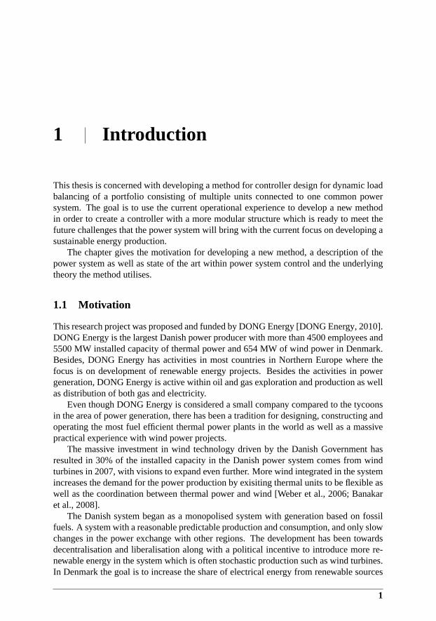
This thesis is concerned with developing a method for controller design for dynamic loadbalancing of a portfolio consisting of multiple units connected to one common powersystem. The goal is to use the current operational experience to develop a new methodin order to create a controller with a more modular structurewhich is ready to meet thefuture challenges that the power system will bring with the current focus on developing asustainable energy production.
The chapter gives the motivation for developing a new method, a description of thepower system as well as state of the art within power system control and the underlyingtheory the method utilises.
1.1 Motivation
This research project was proposed and funded by DONG Energy[DONG Energy, 2010].DONG Energy is the largest Danish power producer with more than 4500 employees and5500 MW installed capacity of thermal power and 654 MW of windpower in Denmark.Besides, DONG Energy has activities in most countries in Northern Europe where thefocus is on development of renewable energy projects. Besides the activities in powergeneration, DONG Energy is active within oil and gas exploration and production as wellas distribution of both gas and electricity.
Even though DONG Energy is considered a small company compared to the tycoonsin the area of power generation, there has been a tradition for designing, constructing andoperating the most fuel efficient thermal power plants in theworld as well as a massivepractical experience with wind power projects.
The massive investment in wind technology driven by the Danish Government hasresulted in 30% of the installed capacity in the Danish powersystem comes from windturbines in 2007, with visions to expand even further. More wind integrated in the systemincreases the demand for the power production by exisiting thermal units to be flexible aswell as the coordination between thermal power and wind [Weber et al., 2006; Banakaret al., 2008].
The Danish system began as a monopolised system with generation based on fossilfuels. A system with a reasonable predictable production and consumption, and only slowchanges in the power exchange with other regions. The development has been towardsdecentralisation and liberalisation along with a political incentive to introduce more re-newable energy in the system which is often stochastic production such as wind turbines.In Denmark the goal is to increase the share of electrical energy from renewable sources
1
Introduction
from 24% in 2005 to 36% in 2025 as found in [Danish Ministry of Transport and Energy,2005].
In 2003 Energinet.dk the Danish Transmission System Operator (TSO) started con-structing a controller to maintain the balance between consumption and production inDenmark. This led to the fact that DONG Energy had to design a controller which couldcommunicate with the TSO and distribute the set point received from the TSO to thethermal power plants. This requirement was expanded withinDONG Energy to includea better coordination of the power plants to minimise the deviations between the actualand sold production within the portfolio. This event was thekickoff the load balancingcontroller within DONG Energy.
The controller started out as an excellent idea implementedas a prototype and hasproved to work well in practice. However, many years of incremental design has led toa structure which is no longer simple and easy to maintain. The purpose of this projectis to take a step back and rethink the design principles for the controller in order to getan easier maintainable controller, and a controller which can cope with the challenges thefuture of the power system is likely to bring.
Since the PhD project started, DONG Energy has formulated a strategy called 85/15,meaning that 85% of the power production should come from carbon dioxide neutralsources within the lifespan of of generation. This is a very challenging vision. There isno grand solution where change of one technology will solve this challenge, it relies onmultiple different techonologies, all cooporating to achieve this goal. An important steptowards this vision is to create a flexible system such that the production and consumptioncan be changed depending on the resources available, such aswind.
One of the candidates for creating flexibility is Virtual Power Plants (VPP). The con-cept pools several, otherwise too small, production and consumption units, such as mul-tiple smaller power plants, wind turbines and heat pumps, and make them behave as oneunit providing yet another means of load balancing. If the VPP concept proves success-ful, an enormous amount of possibilities for load balancingbecomes available, and thusincreasing the importance of this project, rethinking the current load balancing controllerstructure to obtain a more flexible a scalable controller.
Electric vehicles is another topic which catches much attention. The electrical vehi-cles will introduce an additional demand for electricity, but the charging of the vehiclescan be controlled thus providing an additional VPP.
This project has the objective to develop a controller design method for the next gen-eration of load balancing controllers. In order to investigate this objective, the followinghypothesis is formulated
Hypothesis: It is possible to develop a controller design method which can be utilised tosynthesise a controller which fulfils the criteria:
Scalability The controller must be scalable in the number of units participating inthe load balancing control.
Flexibility The controller must be flexible, such that addition of new units andmaintenance of existing ones is possible.
Performance The controller must perform at least as well as the current controllermeasured on some performance criteria.
2
2 Power Systems Control and Electricity Market
1.2 Power Systems Control and Electricity Market
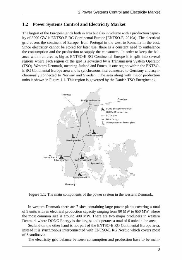
The largest of the European grids both in area but also in volume with a production capac-ity of 3000 GW is ENTSO-E RG Continental Europe [ENTSO-E, 2010a]. The electricalgrid covers the continent of Europe, from Portugal in the west to Romania in the east.Since electricity cannot be stored for later use, there is a constant need to outbalancethe consumption and the production to supply the consumers.In order to keep the bal-ance within an area as big as ENTSO-E RG Continental Europe itis split into severalregions where each region of the grid is governed by a Transmission System Operator(TSO). Western Denmark, meaning Jutland and Funen, is one region within the ENTSO-E RG Continental Europe area and is synchronous interconnected to Germany and asyn-chronously connected to Norway and Sweden. The area along with major productionunits is shown in Figure 1.1. This region is governed by the Danish TSO Energinet.dk.
Studstrupværket
Herningværket
DONG Energy Power Plant
Horns Rev 1
400 KV AC power line
DC Tie Line
Wind farm
Nordjyllandsværket
Other producers Power plant
Norway
Sweden
Esbjergværket Skærbækværket
Enstedværket
Horns Rev 1
Fynsværket
Germany
Figure 1.1: The main components of the power system in the western Denmark.
In western Denmark there are 7 sites containing large power plants covering a totalof 9 units with an electrical production capacity ranging from 80 MW to 650 MW, wherethe most common size is around 400 MW. There are two major producers in westernDenmark where DONG Energy is the largest and operates a totalof 6 units in the area.
Sealand on the other hand is not part of the ENTSO-E RG Continental Europe area,instead it is synchronous interconnected with ENTSO-E RG Nordic which covers mostof Scandinavia.
The electricity grid balance between consumption and production have to be main-
3

Introduction
tained at all times. All the rotating devices connected to the grid, such as generators, havesome energy and thus gives a bit of leeway to maintain the balance. If the consumption islarger than the production, energy will be pulled out of the system, making the generatorsslow down from the usual 50Hz, and thus a drop in the system frequency can be observed.
In order to keep balance between production and consumption, DONG Energy uses amulti hierarchical scheme as shown in Figure 1.2.
Business Planning
(years)
Production planning
(days - weeks)
Measurements
and Servos
(seconds)
Processes
(seconds - minutes)
Units
(minutes - hours)
MM
Balance control
(minutes)
System Level
Plant Level
Figure 1.2: System hierarchy within DONG Energy. The hierarchy consist of a systemlevel which coordinates the units, and a unit level that contains the control hierarchy ofthe individual unit. The time units on the figure show the typical time scale on which thelevel operates.
The upper three levels of the hierarchy are denotedsystem level, meaning that thescope of these levels covers multiple power producing units. On the highest level is thebusiness planning where decisions on building new power plants is taken. It might notseem obvious to include this level when discussing balance between consumption andproduction, but the investment decision is based on the needfor the capacity. Duringplanning and construction, balance control is an essentialpart of the power plant design.
The next level is production planning also known asunit commitment. Productionplanning is static optimisation of load distribution amongpower production units, [Padhy,2004], [Salam, 2007]. Solving the unit commitment problem means determining the com-bination of available generating units and scheduling their respective output to satisfy thereference production, often with a minimisation of cost under the operating constraints en-forced by the power producing portfolio for a specific time - typically from 24 hours up toa week. The optimisation problem is of high dimension and combinatorial in nature, andcan thus be difficult to solve in practice. Results using heuristic methods [Johnson et al.,1971], [Viana et al., 2001], Mixed Integer Programming [Dillon et al., 1978], [Jørgensenet al., 2006], Dynamic Programming [Ayuob and Patton, 1971]and Lagrangian Relax-ation [Aoki et al., 1987], [Shahidehpour and Tong, 1992], have been reported in literature.
Once a solution to the unit comment problem, i.e. a static schedule has been found, the
4
2 Power Systems Control and Electricity Market
load plans are distributed to the generating units. Each unit is responsible for following itsload plan and must handle disturbances etc. locally, implying the necessity of local powerplant controllers, wind farm controllers etc., which is shown as the lower three levels ofthe hierarchy.
The lowest system level is the balance control level. Due to deviations between thepredicted and actual consumption as well as fluctuations in production, this level is addedto give a dynamic correction on system level. Due to the aforementioned increased pro-duction from wind power, the fluctuations in production willincrease in the future, mak-ing this layer even more important. This hierarchy level canbe influenced both by thepower company operating the portfolio of power generating units for minimising the de-viation between sold and actual production, which is only reported in [Jørgensen et al.,2006], and by the TSO in the area, that uses a dynamic feedbackapproach to balance theload in the area. The latter is often referred to as a Automatic Generation Control (AGC).
The problem of designing AGCs to cooperate among multiple regions has been thesubject of much research lately, both regarding optimisation and stability. However, it isoften assumed that the generators within the area function as one generator. For example[Bakken and Grande, 1998] describe how to introduce an AGC inNorway, but the focusis on the main controller rather than the distribution of theerror among the participatinggenerators. Centralised AGC design under constraints is treated in [Hassan et al., 2008]both for single-area and multi-area production, but the area is treated as one generator.In [Venkat et al., 2006; Moon et al., 2000; Tyagi and Srivastava, 2006] decentralisedmodel-based methods for multi-area AGC are developed, but without discussing how todistribute the output from the controller known as the area control error (ACE) amongthe multiple generators in the control area. Focusing on stability, [Azzam and Mohamed,2002] developed a design method for generating a stabilising controller.
[Liu et al., 2003; Chen et al., 2007; Wood and Wollenberg, 1996] describe how todistribute the ACE among the participating generators in the area. [Liu et al., 2003; Chenet al., 2007] deal with control of multiple generators within an area using optimisation-based schemes. However, both treat the problem as a static rather than a dynamic prob-lem. [Wood and Wollenberg, 1996] present an AGC for distributing the ACE to multiplegenerators based on a PI-controller structure with a set of distribution factors to share thecontribution among multiple units. The distribution factors are based on a static optimisa-tion of the system, [Raj, 2006] describes an updated way to use real time prices to updatethe distribution factors. A complete survey can be found in [Shayeghi et al., 2009].
1.2.1 Energy Market and Short Term Load Scheduler
The liberalisation of the power system has created a market which, according to [Jørgensenet al., 2006], includes two types of costumers from the powerproducers’ point of view -The power exchanges and the TSO, the commodities traded in the power market appearin Figure 1.3. The market has influence on the production planning and balance con-trol levels of the hierarchy, where the trades on the market is decisive for the productionplanning and balance control.
The different commodities traded in the market are:
1. Energy Every day an hourly based price for the next 24 hours production is setbased on the producers’ and buyers’ forecasted demands. If the actual production
5

Introduction
TSO
Power Exchange
Power Producer
Commodities
1. Energy2. Reserves
3. Reserve activation
Figure 1.3: Power market commodities.
deviates from the sold production, the TSO will fine the producer, since the TSOmust balance the production by activating reserves. Duringthe day, bilateral tradesamong power producers are allowed through the power exchange as well, to coverforeseen production deficiencies in case of failure.
2. ReservesThe TSO buys power reserves in the form of primary, secondaryandtertiary reserves for a period in time to have capacity to balance out imbalancesbetween the production and consumption. The seller must be able to activate thepower reserve when required throughout the sold period. Thereserves and theirdifferences are described later in this section.
3. Secondary and tertiary reserve activationThe Danish TSO can activate thebought reserves to balance production and consumption in western Denmark. Theseller of the reserves will get extra payment if the reserve is activated. The primaryreserve is governed by the frequency and must be automatically activated in caseof deviations in the system frequency.
Each day on the energy market, which in the Danish case is NordPool [Nord Pool,2010], at noon an auction is run for the forthcoming day. The production companies willsubmit amount and price for the energy production for each hour of the forthcoming day.The distribution companies will submit the consumption andprice they are willing to pay.For each hour an intersection between consumption and production is formed, and thisintersection determines the amount of energy and the price of energy .
After the auction has run, Nord Pool will announce the resultto the participants ofthe auction which includes DONG Energy. The announced result is an amount of energywhich is to be produced each hour. As depicted in Figure 1.4, the sold production is usedby theshort-term load scheduler(STLS) together with weather forecasts, district heatingdemand forecasts and constraints such as minimum amount of biomass fuel. The STLSsolves the unit commitment problem again and the output of the short term load scheduleris a 5-minute based 24 hour ahead schedule for all productionunits that DONG Energyoperates.
Based on the 5-minute based production plan generated by DONG Energy, The TSOgenerates two plans, an hourly and a quarter plan. These plans are used for settlingpayments for deviations.
6
2 Power Systems Control and Electricity Market
TSO
Short-term load
scheduler
(Production Planning)
+
Production plan
Total measured production
Load balancing
controller
+
AGC signal
Filter
Expected
Response
Manual Control
Automatic Control
Measured production of individual units
Sold production
Weather forecast
District heating forecast
+Frequency control
contribution
Reference
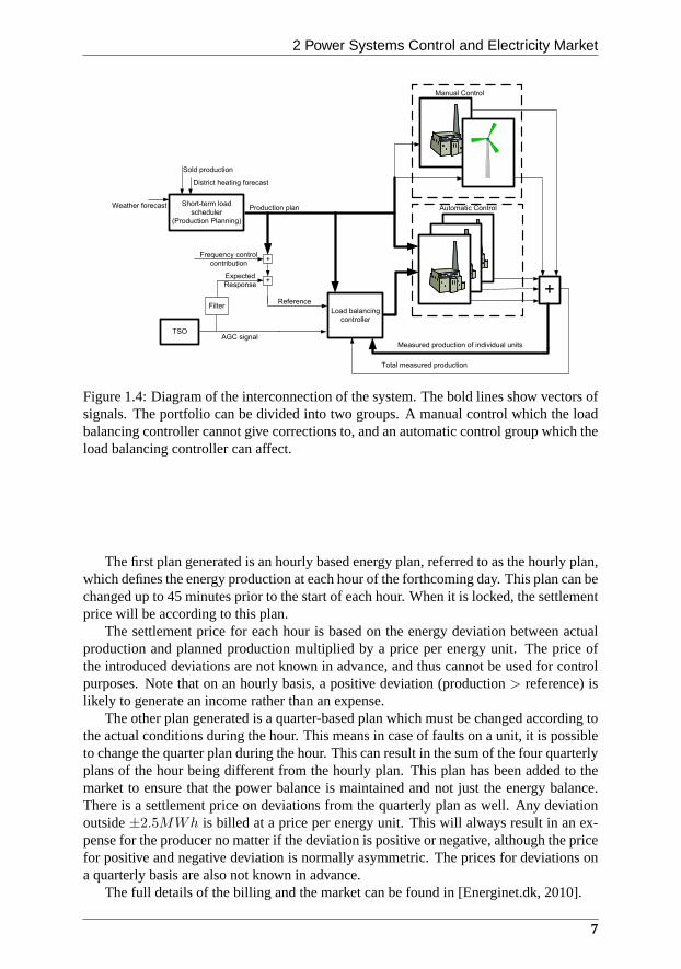
Figure 1.4: Diagram of the interconnection of the system. The bold lines show vectors ofsignals. The portfolio can be divided into two groups. A manual control which the loadbalancing controller cannot give corrections to, and an automatic control group which theload balancing controller can affect.
The first plan generated is an hourly based energy plan, referred to as the hourly plan,which defines the energy production at each hour of the forthcoming day. This plan can bechanged up to 45 minutes prior to the start of each hour. When itis locked, the settlementprice will be according to this plan.
The settlement price for each hour is based on the energy deviation between actualproduction and planned production multiplied by a price perenergy unit. The price ofthe introduced deviations are not known in advance, and thuscannot be used for controlpurposes. Note that on an hourly basis, a positive deviation(production> reference) islikely to generate an income rather than an expense.
The other plan generated is a quarter-based plan which must be changed according tothe actual conditions during the hour. This means in case of faults on a unit, it is possibleto change the quarter plan during the hour. This can result inthe sum of the four quarterlyplans of the hour being different from the hourly plan. This plan has been added to themarket to ensure that the power balance is maintained and notjust the energy balance.There is a settlement price on deviations from the quarterlyplan as well. Any deviationoutside±2.5MWh is billed at a price per energy unit. This will always result in an ex-pense for the producer no matter if the deviation is positiveor negative, although the pricefor positive and negative deviation is normally asymmetric. The prices for deviations ona quarterly basis are also not known in advance.
The full details of the billing and the market can be found in [Energinet.dk, 2010].
7
Introduction
Reserves
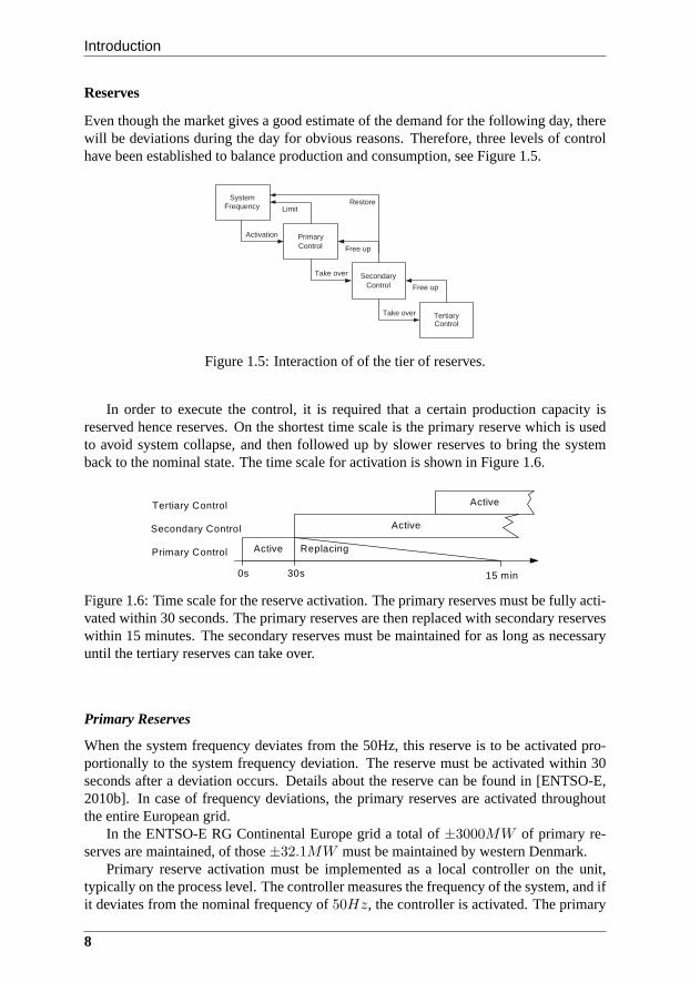
Even though the market gives a good estimate of the demand forthe following day, therewill be deviations during the day for obvious reasons. Therefore, three levels of controlhave been established to balance production and consumption, see Figure 1.5.
System Frequency
Primary Control
Secondary Control
Tertiary Control
Activation
Take over
Take over
Free up
Free up
Limit Restore
Figure 1.5: Interaction of of the tier of reserves.
In order to execute the control, it is required that a certainproduction capacity isreserved hence reserves. On the shortest time scale is the primary reserve which is usedto avoid system collapse, and then followed up by slower reserves to bring the systemback to the nominal state. The time scale for activation is shown in Figure 1.6.
30s 15 min
Active
ActiveTertiary Control
Secondary Control
Primary Control
0s
Active
Replacing
Figure 1.6: Time scale for the reserve activation. The primary reserves must be fully acti-vated within 30 seconds. The primary reserves are then replaced with secondary reserveswithin 15 minutes. The secondary reserves must be maintained for as long as necessaryuntil the tertiary reserves can take over.
Primary Reserves
When the system frequency deviates from the 50Hz, this reserve is to be activated pro-portionally to the system frequency deviation. The reservemust be activated within 30seconds after a deviation occurs. Details about the reservecan be found in [ENTSO-E,2010b]. In case of frequency deviations, the primary reserves are activated throughoutthe entire European grid.
In the ENTSO-E RG Continental Europe grid a total of±3000MW of primary re-serves are maintained, of those±32.1MW must be maintained by western Denmark.
Primary reserve activation must be implemented as a local controller on the unit,typically on the process level. The controller measures thefrequency of the system, and ifit deviates from the nominal frequency of50Hz, the controller is activated. The primary
8
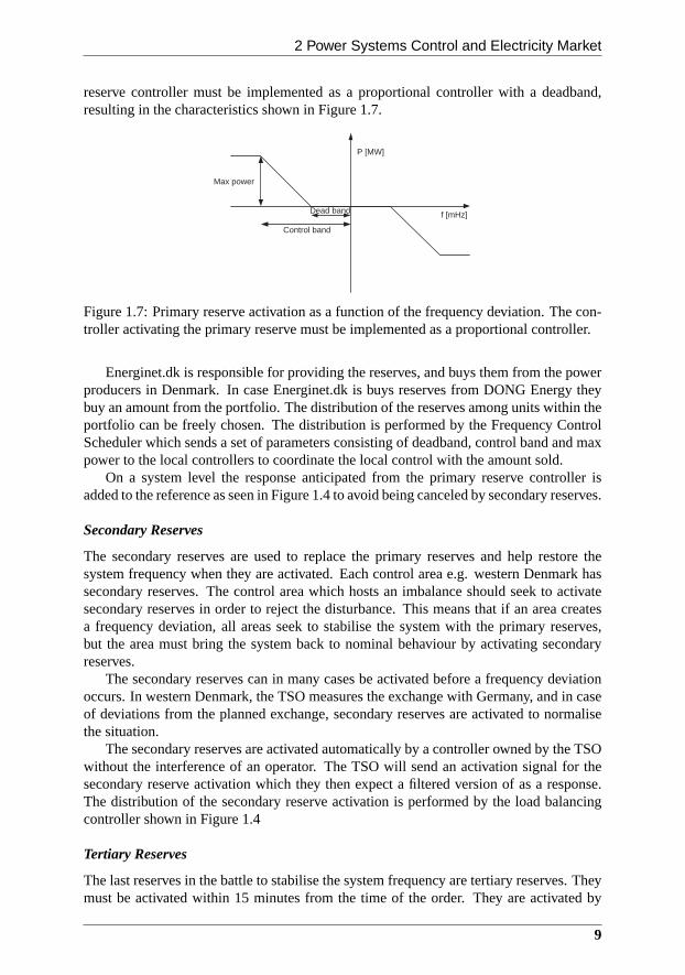
2 Power Systems Control and Electricity Market
reserve controller must be implemented as a proportional controller with a deadband,resulting in the characteristics shown in Figure 1.7.
P [MW]
f [mHz]
Max power
Control band
Dead band
Figure 1.7: Primary reserve activation as a function of the frequency deviation. The con-troller activating the primary reserve must be implementedas a proportional controller.
Energinet.dk is responsible for providing the reserves, and buys them from the powerproducers in Denmark. In case Energinet.dk is buys reservesfrom DONG Energy theybuy an amount from the portfolio. The distribution of the reserves among units within theportfolio can be freely chosen. The distribution is performed by the Frequency ControlScheduler which sends a set of parameters consisting of deadband, control band and maxpower to the local controllers to coordinate the local control with the amount sold.
On a system level the response anticipated from the primary reserve controller isadded to the reference as seen in Figure 1.4 to avoid being canceled by secondary reserves.
Secondary Reserves
The secondary reserves are used to replace the primary reserves and help restore thesystem frequency when they are activated. Each control areae.g. western Denmark hassecondary reserves. The control area which hosts an imbalance should seek to activatesecondary reserves in order to reject the disturbance. Thismeans that if an area createsa frequency deviation, all areas seek to stabilise the system with the primary reserves,but the area must bring the system back to nominal behaviour by activating secondaryreserves.
The secondary reserves can in many cases be activated beforea frequency deviationoccurs. In western Denmark, the TSO measures the exchange with Germany, and in caseof deviations from the planned exchange, secondary reserves are activated to normalisethe situation.
The secondary reserves are activated automatically by a controller owned by the TSOwithout the interference of an operator. The TSO will send anactivation signal for thesecondary reserve activation which they then expect a filtered version of as a response.The distribution of the secondary reserve activation is performed by the load balancingcontroller shown in Figure 1.4
Tertiary Reserves
The last reserves in the battle to stabilise the system frequency are tertiary reserves. Theymust be activated within 15 minutes from the time of the order. They are activated by
9
Introduction
the operator at the TSO by contacting to the operator at the central control room for theenergy generation companies. The additional order of energy will most often be put intothe STLS which will then generate and broadcast a new production plan to the units.
The size of the needed positive reserve is based on theN−1 principle, i.e. there mustbe enough reserves to outbalance a breakdown of the largest unit within the region. Thereserves are asymmetric with+630MW and−160MW which must be fully deliveredwithin 15 minutes.
1.2.2 Load Balancing Controller
The topic of the load balancing controller has already been briefly described in section1.2.1. It serves two purposes; one of them is to distribute the secondary reserve activationsignal among the units. The other purpose is to minimise the deviation between actualand sold power production.
The mechanism for determining the individual units participating in the control mustcontribute is proposed to be a steady state optimisation in [Wood and Wollenberg, 1996].However, due to the conditions in western Denmark, where theboiler units are not usedfor base load, but rather changing load very frequently, thestatic optimisation approachhas been deemed infeasible. Instead, the gains are determined by a logic-based mecha-nism, where each unit is prioritised by the operator for bothnegative and positive correc-tions. The logic then utilises the boiler unit with highest priority first, and after usage allboilers must be returned to the production plan.
Besides the main control loop, there is much logic in the controller for handling bump-less transfer between automatic and manual control and other features in an attempt tomake the controller as optimal as possible. The result is a huge control structure withmany cross couplings.
Figure 1.8 shows the correction signals from the load balancing controller during themorning hours. The correction amount is quite significant.
The problem with the current controller is the complexity ofthe cross couplings,which means that modifying one part of the controller often affects other parts of thecontroller in a way that the designer cannot predict. Thus, while the performance of thecontroller is quite adequate for the existing system, the current structure is not suitedfor portfolios that change structure over time. Furthermore, the complexity of the logicsmakes any form of rigorous stability or performance analysis virtually impossible.
To the author’s knowledge no other load balancing controller for balancing the loadwithin a portfolio has been reported in literature.
Figure 1.4 shows that the portfolio is split in two parts; an automatic control part anda manual control part. DONG Energy has the responsibility todeliver a total productionfrom the portfolio corresponding to the reference. However, not all units have the abilityto communicate with the load balancing controller - they will always be in manual control.But the units that are capable of participating are switchedin and out of automatic controlmode by the operator and the control systems on the unit. The result is a system thatneeds dynamic reconfiguration.
10

2 Power Systems Control and Electricity Market
6 6.2 6.4 6.6 6.8 7 7.2 7.4 7.6 7.8 8
−60
−40
−20
0
20
40
60
80
100
Time [hours]
Cor
rect
ion
[MW
]
Figure 1.8: Example of control signals given by the current controller during the morninghours. Each line shows the corrective control signal to one unit in automatic control. Thecontrol signal for all six units are depicted, but only five participate in the control.
1.2.3 Power Plant Modelling and Control
The planning and dynamic coordination on system level becomes increasingly importantto power systems. In order to cope with the increasing demandfor flexibility, the existingpower plants must be changed from base load to being able to change load fast.
In existing literature there are many detailed models of parts of the energy systemto describe the dynamic behaviour of individual system components, such as [de Mello,1991; Weber and Krueger, 2008].
There is focus both on improving processes in the power plants as well as the mastercontrol level of the unit, i.e. the two upper plant levels in Figure 1.2. [Deprugney andLiters, 2004] reports improvements on the control of the aircontroller. [Mølbak, 1999] re-ports improvement in control of superheater steam temperature control using GeneralisedPredictive control. [Dahl-Soerensen and Solberg, 2009] implement a simple controller toimprove coal mill performance, while [Niemczyk et al., 2009] work on improving non-linear models for use in coal mill control. [Majanne, 2005] works on stabilising the steamtemperature in an industrial power plant where part of the steam is used for other pur-poses than power production using model predictive methods, while [Gibbs et al., 1991]use nonlinear model predictive methods to improve controller design to increase availabil-ity and lower pollution of fossil fired plants. [Mortensen etal., 1998] are concerned withimproving the load following capabilities of the power plants on unit level using LQGmethods, while [Deprugney et al., 2006] useH∞-control. [Welfonder, 1997; Lausterer,1998] both report significant improvements in the the disturbance rejection capabilitiesand load following capabilities of single power plants by using smaller energy buffersin the power plant which can later be repaid, such as the condensate system or turbinethrottling valves.
[Bjerge and Kristoffersen, 2007] share experience designing the controller for an off-
11
Introduction
shore wind farm to be integrated in the current power system.Another issue is the start up of plants where [Franke and Vogelbacher, 2006; Albenesi
et al., 2006] report better automation and faster start up ofthermal power plants andcombined cycle power plants using nonlinear model predtictive methods and nonlinearprogramming. A highly relevant problem when increased flexibility is needed.
Most of the developed controllers and models reported are complex and unsuitedfor making a load balancing controller which covers a large scope and therefore needssimple models to avoid too much complexity. The load balancing controller gives a setpoint to the power production and measures the output from the plant. Therefore, modelsshould be limited to capturing the main dynamics along with the constraints governingthe behaviour, such as the upper and lower production boundsand constraints on the rateof change on the set point.
1.3 State of the Art and Background of Chosen Methodology
This section provides an overview of the state of the art methodology utilised for devel-oping the design method to fulfil the hypothesis.
There are many methods for controlling a MIMO system, such asthe power systemportfolio. Spanning from the current PI-controller structure based on SISO theory incombination with cross couplings and feed forward ([Franklin et al., 2002;Astrom andHagglund, 2006] to mention a few) to more advanced techniquesmodel-based multivari-able controllers like LQR orH∞-control [Skogestad and Postlethwaite, 2005]. The powersystem portfolio is a constrained MIMO system with knowledge of the future reference.Therefore, Model Predictive Control (MPC) is an obvious controller scheme to choose.
In this thesis a linear MPC implementation is utilised whichrequires repeated onlinesolution of constrained linear optimisation problem. Therefore, the some basics of convexoptimisation with the focus on linear programming is covered first in this section.
1.3.1 Convex Optimisation - Linear Programming
In MPC applications the performance and reliability of the optimisation algorithm solv-ing the constrained optimal control problem are important elements, as the optimisationproblem is solved repeatedly online. In linear MPC the performance function is usuallyquadratic, linear, orℓ1-norm based as described previously. Using these performancefunctions leads to a convex optimisation problem as treatedin [Boyd and Vandenberghe,2004].
The performance function used in the controller design method in this project result ina linear constrained optimisation problem, which is a special case of convex programmingand will be described here. A general linear program has the structure
minz
φ = cT z (1.1a)
s.t. Gz ≥ h (1.1b)
with φ ∈ R being the functional to be minimised in order to find optimum,z ∈ Rn
are the free variables which can be manipulated in order to minimiseφ, c ∈ Rn contains
the weights of the free variables, weighing their importance relative to each other.G ∈R
m×n is the constraint matrix, andh ∈ Rm is the affine part of the constraints.
12

3 State of the Art and Background of Chosen Methodology
Checking if a solution is an optimal solution to (1.1) is equivalent to finding a solution(z∗, π∗) to the corresponding Lagranian function
L(z, π) = cT z− πT (Gz ≥ h) (1.2)
with π ∈ Rm being the introduced Lagrange multipliers. If the solution(z∗, π∗) fulfils
theKarush-Kuhn-Tucker(KKT) conditions
∇zL = c−GTπ = 0 (1.3a)
∇πL = Gz− h− s = 0 (1.3b)
siπi = 0 i = 1, 2, . . . ,m (1.3c)
s, π ≥ 0 (1.3d)
with the slack variables defined as
s = Gz− h ≥ 0. (1.4)
then the solutionz∗ is an optimal solution to (1.1) [Nocedal and Wright, 2006].The KKT conditions imply that the first derivative of the Lagranian with respect toz
as well as the first derivative with respect toπ must be zero. Furthermore, element wiseeither the constraint or Lagrange multiplier must be zero.si > 0 means that the proposedsolution is not on the constraint, and thus the constraint does not affect whether or not theoptimum is reach. Ifsi = 0 the constraint is active and the lagrange multiplierπi can bedifferent from zero, and thus affecting (1.3a).
The special property of a linear program is that the solutionwill always be on a vertexof the feasible area. This property can be exploited when finding the solution. In case ofa non unique solution, there will still be a valid solution ona vertex. Illustrated in Figure1.9 is the optimsation problem
minz
φ = −z1 − 2z2 (1.5a)
s.t. z1 ≤ 3 (1.5b)
z2 ≤ 3 (1.5c)
z1 + z2 ≤ 4 (1.5d)
z1 ≥ 0, z2 ≥ 0 (1.5e)
The optimum is shown in the figure and is in an extreme point of the feasible area.There are two main methods to solve this problem, either through theSimplexalgorithm[Dantzig and Thapa, 1997], or through aprimal-dual interior point algorithmsuch asMehrotra’s predictor-corrector algorithm [Mehrotra, 1992; Wright, 1997; Zhang, 1998;Czyzyk et al., 1999; Nocedal and Wright, 2006].
The Simplex algorithm starts at a feasible extreme point of the problem, and travelsalong the edges of the feasible region until it finds optimum.The search will alwayshappen in the direction with the steepest decline. For the example, starting at vertex1there are two possibilities2 or 5. The direction towards2 has the steepest decline. Fromhere the algorithm would go to3 and conclude it to be optimal since following any vertex
13

Introduction
z1
z2 Optimum
1
2 3
4
5
Figure 1.9: Two dimensional linear optimisation problem. The lines show the inequalityconstraints. The dashed lines show the contours of the performance function
would lead to an increase in the objective function. For a detailed mathematical coveringof the algorithm see [Dantzig and Thapa, 1997]. The chosen path is shown in Figure 1.10.The simplex algorithm belongs to the group of active set solvers [Nocedal and Wright,2006], a group which is not restricted to linear programming.
z1
z2 Optimum
1 21
Figure 1.10: Paths to the solution for the interior point andsimplex methods. The blackline shows the interior point method, while the grey line shows the simplex method.
The simplex algorithm is not used in practice, but rather an implementation known asthe revised simplex method [Dantzig and Thapa, 1997] which is more computationally ef-ficient. [Klee and Minty, 1972] showed that the simplex algorithm in worst case needs tovisit all extreme points of the feasible area, and thus growsexponential with the problemsize [Nocedal and Wright, 2006]. In practice the algorithm works well and is widely used.However, this theoretical drawback has lead to the development of alternative methods,such as the interior point methods.
Interior point methods make a search through the interior ofthe feasible area to theoptimum based on the gradient of the performance function. Interior point methods usu-ally uses fewer but more computationally expensive iterations to reach optimum. The
14
3 State of the Art and Background of Chosen Methodology
rule of thumb says that simplex algorithm is faster on small and medium problems, whilethe interior point methods are competitive on large-scale problems [Nocedal and Wright,2006]. However, this is only a rule of thumb. One of the advantages of the interior pointmethod is that the computational complexity lies in calculation of a matrix and a Choleskyfactorisation. And thus it is possible to exploit the structure of the problem and tailor thealgorithm to be efficient on a certain problem. The interior point methods might find anoptimum on an edge instead of a vertex in case of a non unique solution. Figure 1.10shows the path through the interior, it makes a few iterations very close to the goal toconverge completely, which is not shown in the figure.
In an MPC context [Rao et al., 1998] show how to structure a quadratic programarising from linear MPC with a quadratic performance function to make efficient use ofinterior point methods for solving the optimisation problem.
1.3.2 Model Predictive Control
Model Predictive Control (MPC) has successfully been applied in the process industriesfor more than thirty years [Qin and Badgwell, 1997, 2003; Froisy, 2006]. Regarding theuse of MPC within power system, it has been applied both to single elements like boilers[Rossiter et al., 2002; Gibbs et al., 1991] and wind farms [Senjyu et al., 2009]. It has alsobeen applied to coordination of power systems [Venkat et al., 2006; Larson and Karlsson,2003; Negenborn et al., 2009].
MPC refers to a group of control algorithms that makes explicit use of a processmodel to predict future responses from the system. In most implmentations the predictionhorizon is finite and constant, these algorithms are also known as receding horizon con-trollers. At each controller update, measurements from thecontrolled plant are gatheredand predictions are based on these measurements. The predictions are used to evaluatea performance function, and an optimisation is performed which seeks to find the inputsequence optimising the performance function over the chosen horizon. The first input inthe sequence is then applied to the plant, and the procedure is repeated at every controllerupdate.
In this thesis the models used for prediction are linear, though both linear [Muske andRawlings, 1993] and nonlinear models [Allgower et al., 1999; Tennyu et al., 2004] canbe used. An overview of linear MPC is found in [Rossiter, 2003; Maciejowski, 2002;Rawlings and Mayne, 2009] among others.
MPC has a number of strengths, these are the ability to incorporate constraints, usingfuture knowledge and not least handle MIMO systems. The mostimportant ability withMPC is the ability to incorporate constraints both on input,output and internal states ofthe system with MPC. Even though it is denoted linear MPC and it has linear models andaffine constraints, the resulting controller is nonlinear.Compared to a linear controller itis possible to move the system closer to the constraints without increasing the number ofconstraint violations.
Process Control Hierarchy
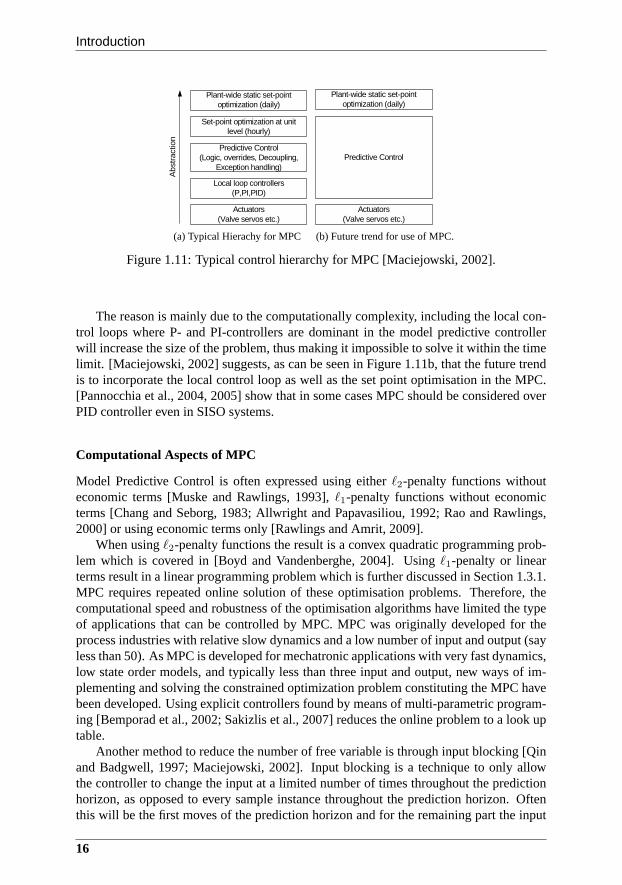
The placement in the control hierarchy is given for the controller in this thesis. However,this section briefly discusses where MPC is usually applied in the hierarchy. MPC isusually found in the middle of the hierarchy, as shown in Figure 1.11a.
15
Introduction
Plant-wide static set-point optimization (daily)
Set-point optimization at unit level (hourly)
Local loop controllers(P,PI,PID)
Predictive Control(Logic, overrides, Decoupling,
Exception handling)
Actuators(Valve servos etc.)
Abs
trac
tion
(a) Typical Hierachy for MPC
Plant-wide static set-point optimization (daily)
Predictive Control
Actuators(Valve servos etc.)
Abstraction
(b) Future trend for use of MPC.
Figure 1.11: Typical control hierarchy for MPC [Maciejowski, 2002].
The reason is mainly due to the computationally complexity,including the local con-trol loops where P- and PI-controllers are dominant in the model predictive controllerwill increase the size of the problem, thus making it impossible to solve it within the timelimit. [Maciejowski, 2002] suggests, as can be seen in Figure 1.11b, that the future trendis to incorporate the local control loop as well as the set point optimisation in the MPC.[Pannocchia et al., 2004, 2005] show that in some cases MPC should be considered overPID controller even in SISO systems.
Computational Aspects of MPC
Model Predictive Control is often expressed using eitherℓ2-penalty functions withouteconomic terms [Muske and Rawlings, 1993],ℓ1-penalty functions without economicterms [Chang and Seborg, 1983; Allwright and Papavasiliou,1992; Rao and Rawlings,2000] or using economic terms only [Rawlings and Amrit, 2009].
When usingℓ2-penalty functions the result is a convex quadratic programming prob-lem which is covered in [Boyd and Vandenberghe, 2004]. Usingℓ1-penalty or linearterms result in a linear programming problem which is further discussed in Section 1.3.1.MPC requires repeated online solution of these optimisation problems. Therefore, thecomputational speed and robustness of the optimisation algorithms have limited the typeof applications that can be controlled by MPC. MPC was originally developed for theprocess industries with relative slow dynamics and a low number of input and output (sayless than 50). As MPC is developed for mechatronic applications with very fast dynamics,low state order models, and typically less than three input and output, new ways of im-plementing and solving the constrained optimization problem constituting the MPC havebeen developed. Using explicit controllers found by means of multi-parametric program-ing [Bemporad et al., 2002; Sakizlis et al., 2007] reduces the online problem to a look uptable.
Another method to reduce the number of free variable is through input blocking [Qinand Badgwell, 1997; Maciejowski, 2002]. Input blocking is atechnique to only allowthe controller to change the input at a limited number of times throughout the predictionhorizon, as opposed to every sample instance throughout theprediction horizon. Oftenthis will be the first moves of the prediction horizon and for the remaining part the input
16
3 State of the Art and Background of Chosen Methodology
is kept constant.Both process control and mechatronic applications use one centralised MPC to control
the system. This is possible because of the low number of input and output as well as therelative low number of states in the model. The system in thisthesis consists of fastdynamics with a large number of controlled inputs and outputs, therefore methods forachieving lower computationally complexity of the controller by exploiting the structureof the problem is treated later in this section.
Models
A common implementation of models in MPC is step or impulse response models. Theadvantage of using these convolution models is that they canrepresent any kind of stabledynamic process [Muske and Rawlings, 1993].
The problem with this formulation is that unstable models cannot be represented.[Morari and Lee, 1991; Eaton and Rawlings, 1992] described ways to encompass thisdeficit by representing the instability as an integrator. [Maciejowski, 2002] gives a wayto decompose the unstable model by using coprime factorisation [Zhou et al., 1996].
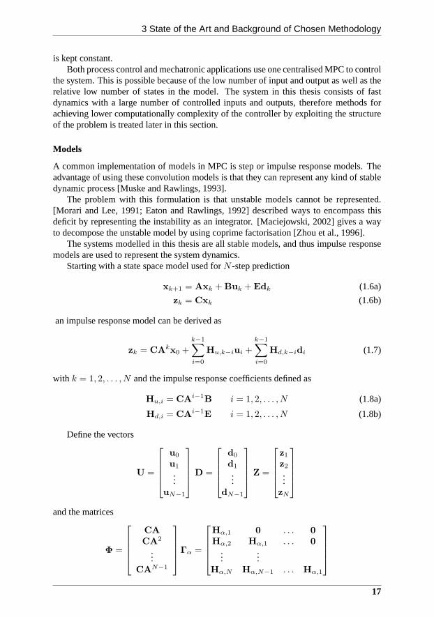
The systems modelled in this thesis are all stable models, and thus impulse responsemodels are used to represent the system dynamics.
Starting with a state space model used forN -step prediction
xk+1 = Axk + Buk + Edk (1.6a)
zk = Cxk (1.6b)
an impulse response model can be derived as
zk = CAkx0 +
k−1∑
i=0
Hu,k−iui +
k−1∑
i=0
Hd,k−idi (1.7)
with k = 1, 2, . . . , N and the impulse response coefficients defined as
Hu,i = CAi−1B i = 1, 2, . . . , N (1.8a)
Hd,i = CAi−1E i = 1, 2, . . . , N (1.8b)
Define the vectors
U =
u0
u1
...uN−1
D =
d0
d1
...dN−1
Z =
z1
z2
...zN
and the matrices
Φ =
CA
CA2
...CAN−1
Γα =
Hα,1 0 . . . 0
Hα,2 Hα,1 . . . 0...
...Hα,N Hα,N−1 . . . Hα,1
17
Introduction
with α ∈ {u, d}. Using (1.7) the stacked output,Z, may be expressed by the linearrelation
Z = Φx0 + ΓuU + ΓdD (1.9)
This model description has eliminated all internal states,except the current, and thus thesize of the matrix relating to controlled input,Γu, is only dependent on the number ofinput, output and prediction horizon.
Output Feedback and Offset-free Tracking
MPC assumes that the state vector is measurable in order to make correct predictions.This is often not the case, so in order to be able to achieve output feedback a state observeris needed, for instance a Kalman Filter [Grewal and Andrews,2008].
If a step disturbance enters the system, the combination controller and observer willresult in a steady state offset from the reference. The same behaviour is exhibited whenthe steady state gain of the model is different from the steady state gain of the system[Maciejowski, 2002].
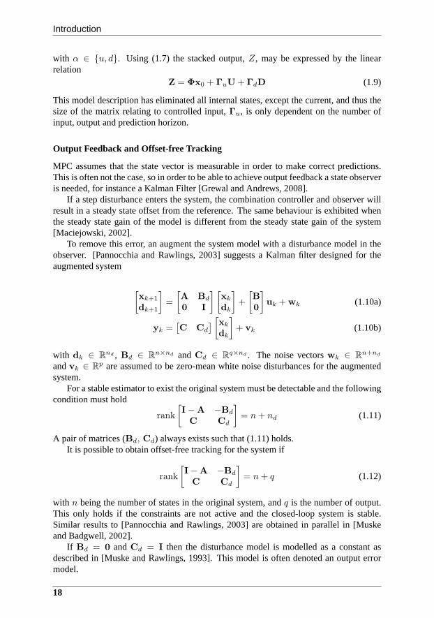
To remove this error, an augment the system model with a disturbance model in theobserver. [Pannocchia and Rawlings, 2003] suggests a Kalman filter designed for theaugmented system
[
xk+1
dk+1
]
=
[
A Bd
0 I
] [
xk
dk
]
+
[
B
0
]
uk + wk (1.10a)
yk =[
C Cd
]
[
xk
dk
]
+ vk (1.10b)
with dk ∈ Rnd , Bd ∈ R
n×nd andCd ∈ Rq×nd . The noise vectorswk ∈ R
n+nd
andvk ∈ Rp are assumed to be zero-mean white noise disturbances for theaugmented
system.For a stable estimator to exist the original system must be detectable and the following
condition must hold
rank
[
I−A −Bd
C Cd
]
= n+ nd (1.11)
A pair of matrices (Bd, Cd) always exists such that (1.11) holds.It is possible to obtain offset-free tracking for the systemif
rank
[
I−A −Bd
C Cd
]
= n+ q (1.12)
with n being the number of states in the original system, andq is the number of output.This only holds if the constraints are not active and the closed-loop system is stable.Similar results to [Pannocchia and Rawlings, 2003] are obtained in parallel in [Muskeand Badgwell, 2002].
If Bd = 0 andCd = I then the disturbance model is modelled as a constant asdescribed in [Muske and Rawlings, 1993]. This model is oftendenoted an output errormodel.
18

3 State of the Art and Background of Chosen Methodology
Controller Tuning
A model predictive controller must be tuned like most other controller. The performanceis based on the values of the weight functions in the performance function and the pre-diction horizon as well as the observer, for instance the covariance matrices in a Kalmanfilter. Depending on the problem size, this gives quite a number of free design variables.
In practice, for all types of controllers tuning, the controller such that the systemsbehaves “right” is often a matter of trial and error.
In some cases the weight matrices may be given, but in most cases this is a task for thecontroller designer. There are methods to aid controller tuning such as loop transfer re-covery [Doyle and Stein, 1981], and least-squares methods for estimating autocovarianceon noise [Akesson et al., 2007; Odelson et al., 2006; Rajamani and Rawlings, 2009].
1.3.3 Hierarchical Control and Reconfigurable Systems
Decomposing the control problem into smaller problems, whether the structure is decen-tralised without communication between local controllers[Elliott and Rasmussen, 2008;Acar, 1995; Magni and Scattolini, 2006; Raimondo et al., 2007], distributed where thelocal controllers communicate [Mercangoz and Doyle III, 2007; Jia and Krogh, 2001;Dunbar, 2007] or hierarchical, as used in this thesis, can serve many purposes.
Complexity of power plants, power systems and most other process and traffic net-works have increased due to a wish to optimise them. The systems often consist of mul-tiple units or subsystems interacting, and it can be difficult to control with a centralisedcontrol structure. Reasons for not pursuing a centralised solution could be that the con-trolled system is spread over a physical area where communication could be expensivein resources such as communication bandwidth of power consumption as in multi robotcoordination [Keviczky et al., 2008], or communication delays as in multi area automaticgeneration control [Venkat et al., 2008]. Other reasons fordecomposition of the controlis to achieve robustness, reliability or reconfigurabilityof the subsystems without havingto redesign the whole controller or to achieve a lower computationally complexity.
The overall structure of the power system portfolio controlis hierarchical, but on theplant level, especially in the units, numerous examples of both decentralised and dis-tributed controllers can be found. The main focus on the restof the section is on MPCimplementations of hierarchical control and reconfigurable control.
A good classification and review of the subject of the area canbe found in [Scattolini,2009].
There are many variants of hierarchies, the main structure of the power system portfo-lio is a multi layered hierarchy. However, this thesis treats two layer hierarchical controlfor coordination. The idea of hierarchical control and the design of coordinators hasbeen studied for a long time [Mesarovic et al., 1970]. The basic idea is that the systemcomprises a set of subsystems under local control with some interaction either through acommon goal or through dynamic interaction.
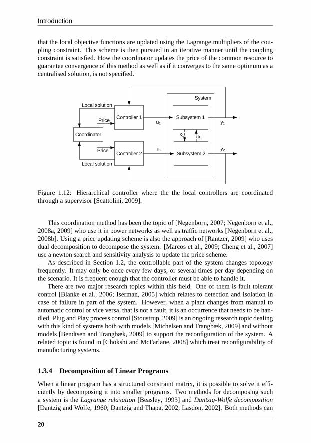
The basic idea is described in [Scattolini, 2009] and shown in Figure 1.12. For eachlocal system an MPC optimises the local performance function under local constraints.If the local solution for each subsystem satisfies the constraints that couples the subsys-tems together, the solution is accepted. If this is not the case, the coordinator will updatethe local control objective based on the coupling constraint. [Scattolini, 2009] suggests
19
Introduction
that the local objective functions are updated using the Lagrange multipliers of the cou-pling constraint. This scheme is then pursued in an iterative manner until the couplingconstraint is satisfied. How the coordinator updates the price of the common resource toguarantee convergence of this method as well as if it converges to the same optimum as acentralised solution, is not specified.
Subsystem 1
Subsystem 2
Controller 1
Controller 2
u1
u2
y1
y2
System
Coordinator
Local solution
Price
Price
Local solution
x2x1
Figure 1.12: Hierarchical controller where the the local controllers are coordinatedthrough a supervisor [Scattolini, 2009].
This coordination method has been the topic of [Negenborn, 2007; Negenborn et al.,2008a, 2009] who use it in power networks as well as traffic networks [Negenborn et al.,2008b]. Using a price updating scheme is also the approach of[Rantzer, 2009] who usesdual decomposition to decompose the system. [Marcos et al.,2009; Cheng et al., 2007]use a newton search and sensitivity analysis to update the price scheme.
As described in Section 1.2, the controllable part of the system changes topologyfrequently. It may only be once every few days, or several times per day depending onthe scenario. It is frequent enough that the controller mustbe able to handle it.
There are two major research topics within this field. One of them is fault tolerantcontrol [Blanke et al., 2006; Iserman, 2005] which relates to detection and isolation incase of failure in part of the system. However, when a plant changes from manual toautomatic control or vice versa, that is not a fault, it is an occurrence that needs to be han-dled. Plug and Play process control [Stoustrup, 2009] is an ongoing research topic dealingwith this kind of systems both with models [Michelsen and Trangbæk, 2009] and withoutmodels [Bendtsen and Trangbæk, 2009] to support the reconfiguration of the system. Arelated topic is found in [Chokshi and McFarlane, 2008] which treat reconfigurability ofmanufacturing systems.
1.3.4 Decomposition of Linear Programs
When a linear program has a structured constraint matrix, it is possible to solve it effi-ciently by decomposing it into smaller programs. Two methods for decomposing sucha system is theLagrange relaxation[Beasley, 1993] andDantzig-Wolfe decomposition[Dantzig and Wolfe, 1960; Dantzig and Thapa, 2002; Lasdon, 2002]. Both methods can
20
3 State of the Art and Background of Chosen Methodology
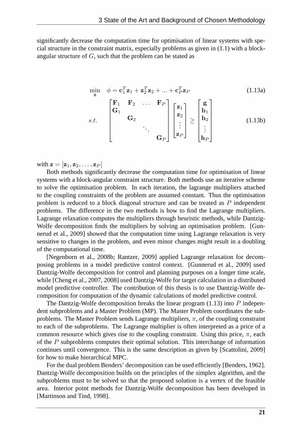
significantly decrease the computation time for optimisation of linear systems with spe-cial structure in the constraint matrix, especially problems as given in (1.1) with a block-angular structure ofG, such that the problem can be stated as
minz
φ = cT1 z1 + zT
2 z2 + ...+ cTP zP (1.13a)
s.t.
F1 F2 . . . FP
G1
G2
. . .GP
z1
z2
...zP
≥
g
h1
h2
...hP
(1.13b)
with z = [z1, z2, . . . , zP ]Both methods significantly decrease the computation time for optimisation of linear
systems with a block-angular constraint structure. Both methods use an iterative schemeto solve the optimisation problem. In each iteration, the lagrange multipliers attachedto the coupling constraints of the problem are assumed constant. Thus the optimisationproblem is reduced to a block diagonal structure and can be treated asP independentproblems. The difference in the two methods is how to find the Lagrange multipliers.Lagrange relaxation computes the multipliers through heuristic methods, while Dantzig-Wolfe decomposition finds the multipliers by solving an optimisation problem. [Gun-nerud et al., 2009] showed that the computation time using Lagrange relaxation is verysensitive to changes in the problem, and even minor changes might result in a doublingof the computational time.
[Negenborn et al., 2008b; Rantzer, 2009] applied Lagrange relaxation for decom-posing problems in a model predictive control context. [Gunnerud et al., 2009] usedDantzig-Wolfe decomposition for control and planning purposes on a longer time scale,while [Cheng et al., 2007, 2008] used Dantzig-Wolfe for target calculation in a distributedmodel predictive controller. The contribution of this thesis is to use Dantzig-Wolfe de-composition for computation of the dynamic calculations ofmodel predictive control.
The Dantzig-Wolfe decomposition breaks the linear program(1.13) intoP indepen-dent subproblems and a Master Problem (MP). The Master Problem coordinates the sub-problems. The Master Problem sends Lagrange multipliers,π, of the coupling constraintto each of the subproblems. The Lagrange multiplier is ofteninterpreted as a price of acommon resource which gives rise to the coupling constraint. Using this price,π, eachof theP subproblems computes their optimal solution. This interchange of informationcontinues until convergence. This is the same description as given by [Scattolini, 2009]for how to make hierarchical MPC.
For the dual problem Benders’ decomposition can be used efficiently [Benders, 1962].Dantzig-Wolfe decomposition builds on the principles of the simplex algorithm, and thesubproblems must to be solved so that the proposed solution is a vertex of the feasiblearea. Interior point methods for Dantzig-Wolfe decomposition has been developed in[Martinson and Tind, 1998].
21

Introduction
1.4 Outline of Thesis
This thesis is made as a collection of publications and is divided into two parts. The firstpart, which has already begun with a system description and state of the art in Chapter1, consists of an introduction and state of the art. The next chapter, Chapter 2, describesthe design method developed through the contributions which fulfil the criteria of themain hypothesis as presented in Section 1.1. A summary of thecontributions is given inChapter 3. Part 1 ends with a conclusion and suggestions for future work presented inChapter 4.
The second part is the presentation of the six publications made during the project andpresented in the following order:
Paper A [Edlund et al., 2009a] Shows that the controller structure of the currentcontroller is internally unstable, unless the gains distributing the control actionswere chosen carefully. This research was driven by an observed problem where thepower plant in control drifted away from the production plan. This paper serves asa motivation for developing a new and more stringent design method.
Paper B [Edlund et al., 2008] Introduces model predictive control for controllinga power plant portfolio. This paper gives a preliminary indication that MPC is aviable option to base a design method upon.
Paper C [Edlund et al., 2009b] MPC relies on models, and as the scope broad-ens, the required fidelity of the models are lowered. Therefore, it was necessaryto develop simple models for use in a model based portfolio controller. This papercovers the modeling of different possibilities to change load within the portfolio.These possibilities are termed effectuators. The paper includes models for fourdifferent effectuators; boiler load, district heating, condensate throttling and windturbines. Only the boiler load unit is currently operational in the portfolio.
Paper D [Edlund et al., 2009c] In this paper a primal-dual interior point algo-rithm based on Mehrotra’s predictor-corrector algorithm is tailored to the controlof a single boiler load effectuator. Even though the optimisation problem in thecontroller is decomposed, an efficient solution strategy still relies on solving thederived subproblems fast. This paper exploits the structure of the subproblem toreduce the number of calculations.
Paper E [Edlund and Jørgensen, nd]Introduces Dantzig-Wolfe decompositionfor solving the dynamic part of the model predictive controller. A thorough descrip-tion of the algorithm is presented. The main result of the paper is the experimentalresults showing linear scalability of the algorithm as a function of the number ofeffectuators.
Paper F [Edlund et al., nd] This paper gives an overview of the complete designmethod, including the handling of switching effectuators in and out of automaticcontrol. A simulation based comparison with the currently implemented controlleris presented based on the actual scenario of a month of portfolio operation.
22

2 Design Method
The load balance controller as seen in Figure 1.4 is the focusof this thesis. The objectiveof the controller is to minimise deviations between sold andactual production as well asactivating secondary reserves when ordered by the TSO.
In order to accept the main hypothesis from Section 1.1, the design method for thenew load balancing controller must result in a a controller that meets the criteria:
Scalability Is scalable in the number of units it can coordinate.
Flexibility Must be flexible, so that addition of new units and maintenance ofexisting units is possible. This means that the design must have a modular struc-ture with good encapsulation of information and clear communication interfacesbetween modules.
Performance Perform as least on par with the current controller measuredonsome performance criteria.
Balance between the production and consumption is currently maintained by chang-ing the production, but in some cases consumption could be changed as well to achievethe goal. For the sake of generalisation all power producingand power consuming unitsthat are capable of participating in load balancing controlare termedeffectuatorswhichhas the definition:
Definition 1. An effectuator is a process or part of a process in a power system that rep-resents control actions with associated dynamics and actuation costs allowing the poweroutput to be manipulated.
2.1 Proposed Controller Structure
The structure of the proposed controller is a two layer hierarchical structure as shown inFigure 2.1. All parts referring to the individual effectuators in the controller are placedin the lower layer separated from one another, allowing themto be modified, removed oradding new ones without affecting the other units. Above is acoordination layer coordi-nating the units in question to achieve the portfolio goal ofminimising deviations.
Model Predictive Control (MPC) has been chosen as the controller scheme, sincethe system is a constrained MIMO system where knowledge of the future references areavailable.
The design framework relies on a set of assumptions:
23

Design Method
Coordinator
Unit P�
Load balancing controller
State estimator
rport
rPUnit 1 Unit 2
r1
AGC signal
xport
y1 y2 yP
u1 u2 uPx1 x2 xP
r2
yport
Figure 2.1: Sketch of the modular structure of the load balancing controller. Commu-nication with the individual effectuator is handled by the independent subsystems, andportfolio communication is handled on the upper layer of thehierarchy. ri is the refer-ence to effectuatori ∈ {1, 2, . . . , P}, xi is the state estimate,yi is the measured output,andui is the controller correction. For the portfolio there is a referencerport, state esti-matexport and a total measured productionyport. The referencesri andrport come fromthe STLS as seen in Figure 1.4.
• The effectuators can be modelled as independent of each other, so that a change inone effectuator does not directly affect another effectuator.
• The effectuators can be modelled as a linear dynamic model with affine constraints.The investigated models in [Edlund et al., 2009b] can all, with minor modifications,be modelled with the structure shown in Figure 2.2. However,other kinds of linear
Linear process
dynam icsu i y i
M in/m ax Rate lim it M in/m ax
Figure 2.2: General structure of the effectuators
input, output and state constraints fit into the modelling framework as well.
• The underlying optimisation problem in the MPC can be statedas a linear program,which means the corresponding objective function must consist of linear andℓ1-norm elements.
24

1 Proposed Controller Structure
Each effectuator in the lower layer of the hierarchy contains a constrained linearmodel and an objective function for the optimal operation ofthe effectuator which to-gether form a constrained linear programming problem. Furthermore, it contains all com-munication with the physical unit. The information that must be sent to the upper layer ishow the output of the effectuator will affect the portfolio output, meaning a prediction ofthe power production/consumption of the unit.
The upper layer contains a constrained linear model of the portfolio excluding the in-dividually modelled effectuators, as well as an objective function of the optimal operationof the portfolio. The upper layer also handles communication with surrounding systems,for instance obtaining the portfolio reference (the load schedule).
2.1.1 Solving the Optimisation Problem
The hierarchical structure encapsulates the information referring to each unit. However,one challenge persists: MPC relies on solving an optimisation problem at each sample.This is a challenge of the MPC framework, since solving the optimisation problem usu-ally grows cubically with the size of the problem. Therefore, one of the design challengeshas been to create an optimisation problem which can be encapsulated in the same hier-archical structure as well as being scalable.
To solve the optimisation problem, a Dantzig-Wolfe decomposition approach has beenapplied [Dantzig and Wolfe, 1960; Dantzig and Thapa, 2002].The decomposition tech-nique has been adapted to the MPC context in [Edlund and Jørgensen, nd] where detailsof the algorithm are also described.
Dantzig-Wolfe decomposition can only be applied to linear problems. The perfor-mance function for the whole problem is assumed to be chosen as a mixture of linear andℓ1-norm terms which can be rewritten into a linear program suitable for Dantzig-Wolfedecomposition.
An important consequence of this forced choice of performance function and con-straints is the solution, i.e. the point where the performance function attains its extremum,must either be at an extreme point of the feasible set, or the solution of an unconstrainedproblem.
When the optimisation problem is composed from the effectuator optimsation prob-lems and the portfolio optimisation problem, it can be rewritten into a linear program withthe structure
minz
φ = cT1 z1 + cT
2 z2 + ...+ cTP zP (2.1a)
s.t.
F1 F2 . . . FP
G1
G2
. . .GP
z1
z2
...zP
≥
g
h1
h2
...hP
. (2.1b)
with z = [z1, z2, . . . zP ] ∈ Rn, zi ∈ R
ni , φ ∈ R, Fi ∈ Rm×ni , Gi ∈ R
pi×ni , g ∈ Rm
andh ∈ Rpi . φ is the functional which needs to be minimised in order to find optimum,zi
are the free variables,ci are weight factors, weighing the importance of the correspondingzi. The constraint matrix has a block-angular structure wherethe block diagonal elements
25
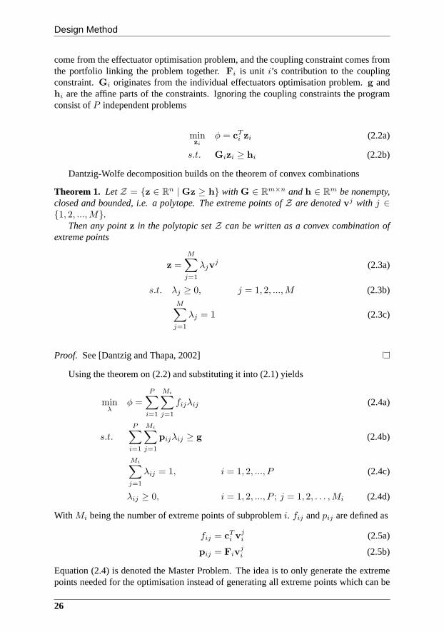
Design Method
come from the effectuator optimisation problem, and the coupling constraint comes fromthe portfolio linking the problem together.Fi is unit i’s contribution to the couplingconstraint.Gi originates from the individual effectuators optimisationproblem. g andhi are the affine parts of the constraints. Ignoring the coupling constraints the programconsist ofP independent problems
minzi
φ = cTi zi (2.2a)
s.t. Gizi ≥ hi (2.2b)
Dantzig-Wolfe decomposition builds on the theorem of convex combinations
Theorem 1. LetZ = {z ∈ Rn |Gz ≥ h} with G ∈ R
m×n andh ∈ Rm be nonempty,
closed and bounded, i.e. a polytope. The extreme points ofZ are denotedvj with j ∈{1, 2, ...,M}.
Then any pointz in the polytopic setZ can be written as a convex combination ofextreme points
z =
M∑
j=1
λjvj (2.3a)
s.t. λj ≥ 0, j = 1, 2, ...,M (2.3b)M∑
j=1
λj = 1 (2.3c)
Proof. See [Dantzig and Thapa, 2002]
Using the theorem on (2.2) and substituting it into (2.1) yields
minλ
φ =
P∑
i=1
Mi∑
j=1
fijλij (2.4a)
s.t.P
∑
i=1
Mi∑
j=1
pijλij ≥ g (2.4b)
Mi∑
j=1
λij = 1, i = 1, 2, ..., P (2.4c)
λij ≥ 0, i = 1, 2, ..., P ; j = 1, 2, . . . ,Mi (2.4d)
With Mi being the number of extreme points of subproblemi. fij andpij are defined as
fij = cTi v
ji (2.5a)
pij = Fivji (2.5b)
Equation (2.4) is denoted the Master Problem. The idea is to only generate the extremepoints needed for the optimisation instead of generating all extreme points which can be
26
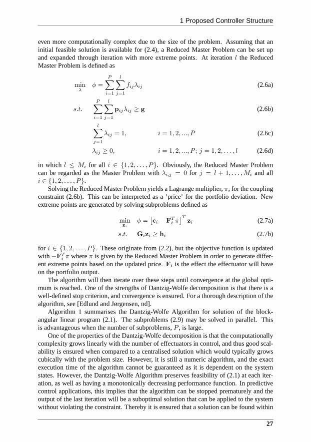
1 Proposed Controller Structure
even more computationally complex due to the size of the problem. Assuming that aninitial feasible solution is available for (2.4), a ReducedMaster Problem can be set upand expanded through iteration with more extreme points. Atiteration l the ReducedMaster Problem is defined as
minλ
φ =P
∑
i=1
l∑
j=1
fijλij (2.6a)
s.t.
P∑
i=1
l∑
j=1
pijλij ≥ g (2.6b)
l∑
j=1
λij = 1, i = 1, 2, ..., P (2.6c)
λij ≥ 0, i = 1, 2, ..., P ; j = 1, 2, . . . , l (2.6d)
in which l ≤ Mi for all i ∈ {1, 2, . . . , P}. Obviously, the Reduced Master Problemcan be regarded as the Master Problem withλi,j = 0 for j = l + 1, . . . ,Mi and alli ∈ {1, 2, . . . , P}.
Solving the Reduced Master Problem yields a Lagrange multiplier, π, for the couplingconstraint (2.6b). This can be interpreted as a ’price’ for the portfolio deviation. Newextreme points are generated by solving subproblems definedas
minzi
φ =[
ci − FTi π
]Tzi (2.7a)
s.t. Gizi ≥ hi (2.7b)
for i ∈ {1, 2, . . . , P}. These originate from (2.2), but the objective function is updatedwith −FT
i π whereπ is given by the Reduced Master Problem in order to generate differ-ent extreme points based on the updated price.Fi is the effect the effectuator will haveon the portfolio output.
The algorithm will then iterate over these steps until convergence at the global opti-mum is reached. One of the strengths of Dantzig-Wolfe decomposition is that there is awell-defined stop criterion, and convergence is ensured. For a thorough description of thealgorithm, see [Edlund and Jørgensen, nd].
Algorithm 1 summarises the Dantzig-Wolfe Algorithm for solution of the block-angular linear program (2.1). The subproblems (2.9) may be solved in parallel. Thisis advantageous when the number of subproblems,P , is large.
One of the properties of the Dantzig-Wolfe decomposition isthat the computationallycomplexity grows linearly with the number of effectuators in control, and thus good scal-ability is ensured when compared to a centralised solution which would typically growscubically with the problem size. However, it is still a numeric algorithm, and the exactexecution time of the algorithm cannot be guaranteed as it isdependent on the systemstates. However, the Dantzig-Wolfe Algorithm preserves feasibility of (2.1) at each iter-ation, as well as having a monotonically decreasing performance function. In predictivecontrol applications, this implies that the algorithm can be stopped prematurely and theoutput of the last iteration will be a suboptimal solution that can be applied to the systemwithout violating the constraint. Thereby it is ensured that a solution can be found within
27
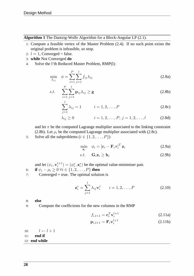
Design Method
Algorithm 1 The Dantzig-Wolfe Algorithm for a Block-Angular LP (2.1).
1: Compute a feasible vertex of the Master Problem (2.4). If no such point exists theoriginal problem is infeasible, so stop.
2: l = 1, Converged = false.3: while Not Convergeddo4: Solve the l’th Reduced Master Problem, RMP(l):
minλij
φ =
P∑
i=1
l∑
j=1
fijλij (2.8a)
s.t.
P∑
i=1
l∑
j=1
pijλij ≥ g (2.8b)
l∑
j=1
λij = 1 i = 1, 2, . . . , P (2.8c)
λij ≥ 0 i = 1, 2, . . . , P ; j = 1, 2, . . . , l (2.8d)
and letπ be the computed Lagrange multiplier associated to the linking constraint(2.8b). Letρi be the computed Lagrange multiplier associated with (2.8c).
5: Solve all the subproblems (i ∈ {1, 2, . . . , P})
minzi
φi = [ci − Fiπ]T
zi (2.9a)
s.t. Gizi ≥ hi (2.9b)
and let(ψi,vl+1i ) = (φ∗i , z
∗i ) be the optimal value-minimiser pair.
6: if ψi − ρi ≥ 0 ∀i ∈ {1, 2, . . . , P} then7: Converged = true. The optimal solution is
z∗i =
l∑
j=1
λijvji i = 1, 2, . . . , P (2.10)
8: else9: Compute the coefficients for the new columns in the RMP
fi,l+1 = cTi vl+1
i (2.11a)
pi,l+1 = Fivl+1i (2.11b)
10: l← l + 111: end if12: end while
28
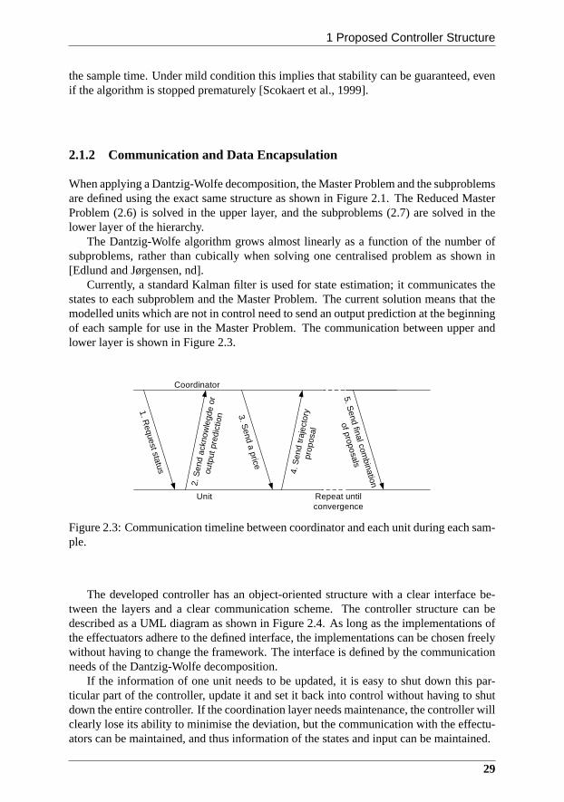
1 Proposed Controller Structure
the sample time. Under mild condition this implies that stability can be guaranteed, evenif the algorithm is stopped prematurely [Scokaert et al., 1999].
2.1.2 Communication and Data Encapsulation
When applying a Dantzig-Wolfe decomposition, the Master Problem and the subproblemsare defined using the exact same structure as shown in Figure 2.1. The Reduced MasterProblem (2.6) is solved in the upper layer, and the subproblems (2.7) are solved in thelower layer of the hierarchy.
The Dantzig-Wolfe algorithm grows almost linearly as a function of the number ofsubproblems, rather than cubically when solving one centralised problem as shown in[Edlund and Jørgensen, nd].
Currently, a standard Kalman filter is used for state estimation; it communicates thestates to each subproblem and the Master Problem. The current solution means that themodelled units which are not in control need to send an outputprediction at the beginningof each sample for use in the Master Problem. The communication between upper andlower layer is shown in Figure 2.3.
Coordinator
Unit
1. Request status
2. S
end
ackn
owle
gde
or
outp
ut p
redi
ctio
n 3. Send a price
4. S
end
traj
ecto
ry
prop
osal
Repeat until convergence
5. Send final com
bination
of proposals
Figure 2.3: Communication timeline between coordinator and each unit during each sam-ple.
The developed controller has an object-oriented structurewith a clear interface be-tween the layers and a clear communication scheme. The controller structure can bedescribed as a UML diagram as shown in Figure 2.4. As long as the implementations ofthe effectuators adhere to the defined interface, the implementations can be chosen freelywithout having to change the framework. The interface is defined by the communicationneeds of the Dantzig-Wolfe decomposition.
If the information of one unit needs to be updated, it is easy to shut down this par-ticular part of the controller, update it and set it back intocontrol without having to shutdown the entire controller. If the coordination layer needsmaintenance, the controller willclearly lose its ability to minimise the deviation, but the communication with the effectu-ators can be maintained, and thus information of the states and input can be maintained.
29
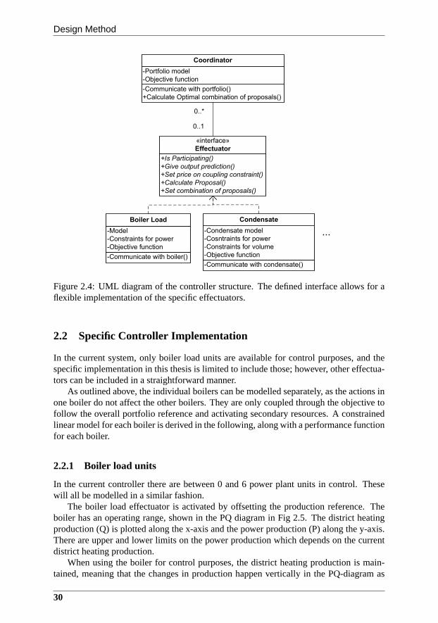
Design Method
-Communicate with portfolio()
+Calculate Optimal combination of proposals()
-Portfolio model
-Objective function
Coordinator
+Is Participating()
+Give output prediction()
+Set price on coupling constraint()
+Calculate Proposal()
+Set combination of proposals()
«interface»
Effectuator
-Communicate with boiler()
-Model
-Constraints for power
-Objective function
Boiler Load
-Communicate with condensate()
-Condensate model
-Cosntraints for power
-Constraints for volume
-Objective function
Condensate
...
0..*
0..1
Figure 2.4: UML diagram of the controller structure. The defined interface allows for aflexible implementation of the specific effectuators.
2.2 Specific Controller Implementation
In the current system, only boiler load units are available for control purposes, and thespecific implementation in this thesis is limited to includethose; however, other effectua-tors can be included in a straightforward manner.
As outlined above, the individual boilers can be modelled separately, as the actions inone boiler do not affect the other boilers. They are only coupled through the objective tofollow the overall portfolio reference and activating secondary resources. A constrainedlinear model for each boiler is derived in the following, along with a performance functionfor each boiler.
2.2.1 Boiler load units
In the current controller there are between 0 and 6 power plant units in control. Thesewill all be modelled in a similar fashion.
The boiler load effectuator is activated by offsetting the production reference. Theboiler has an operating range, shown in the PQ diagram in Fig 2.5. The district heatingproduction (Q) is plotted along the x-axis and the power production (P) along the y-axis.There are upper and lower limits on the power production which depends on the currentdistrict heating production.
When using the boiler for control purposes, the district heating production is main-tained, meaning that the changes in production happen vertically in the PQ-diagram as
30
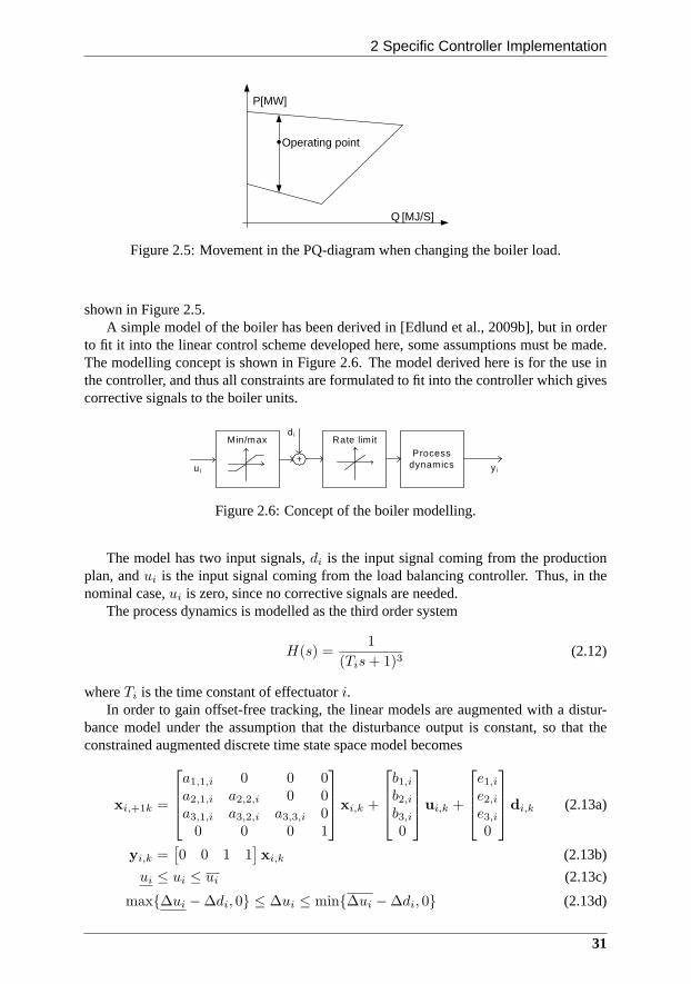
2 Specific Controller Implementation
P[MW]
Q [MJ/S]
Operating point
Figure 2.5: Movement in the PQ-diagram when changing the boiler load.
shown in Figure 2.5.A simple model of the boiler has been derived in [Edlund et al., 2009b], but in order
to fit it into the linear control scheme developed here, some assumptions must be made.The modelling concept is shown in Figure 2.6. The model derived here is for the use inthe controller, and thus all constraints are formulated to fit into the controller which givescorrective signals to the boiler units.
u i y i
Process dynamics
Min/max Rate lim it
+
d i
Figure 2.6: Concept of the boiler modelling.
The model has two input signals,di is the input signal coming from the productionplan, andui is the input signal coming from the load balancing controller. Thus, in thenominal case,ui is zero, since no corrective signals are needed.
The process dynamics is modelled as the third order system
H(s) =1
(Tis+ 1)3(2.12)
whereTi is the time constant of effectuatori.In order to gain offset-free tracking, the linear models areaugmented with a distur-
bance model under the assumption that the disturbance output is constant, so that theconstrained augmented discrete time state space model becomes
xi,+1k =
a1,1,i 0 0 0a2,1,i a2,2,i 0 0a3,1,i a3,2,i a3,3,i 0
0 0 0 1
xi,k +
b1,i
b2,i
b3,i
0
ui,k +
e1,i
e2,i
e3,i
0
di,k (2.13a)
yi,k =[
0 0 1 1]
xi,k (2.13b)
ui ≤ ui ≤ ui (2.13c)
max{∆ui −∆di, 0} ≤ ∆ui ≤ min{∆ui −∆di, 0} (2.13d)
31
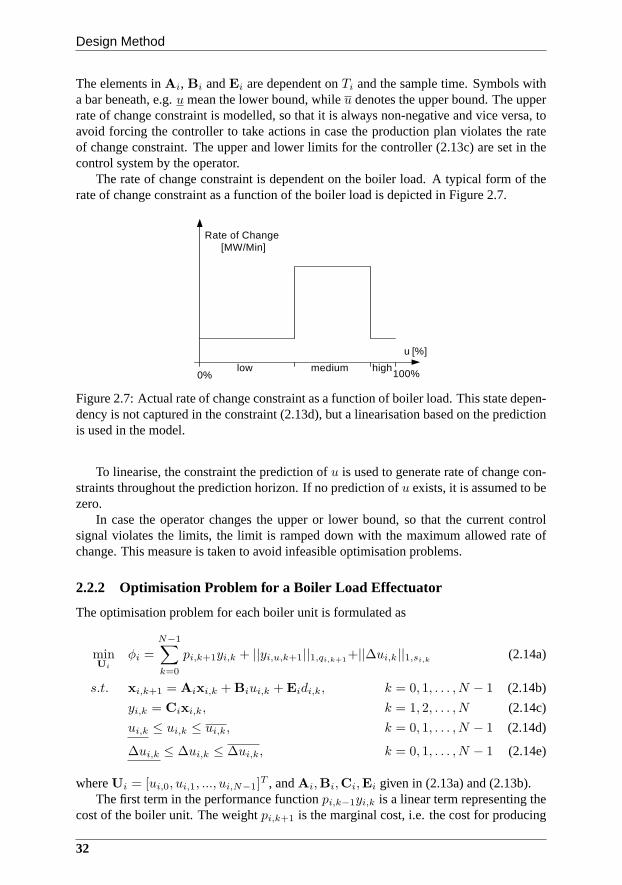
Design Method
The elements inAi, Bi andEi are dependent onTi and the sample time. Symbols witha bar beneath, e.g.u mean the lower bound, whileu denotes the upper bound. The upperrate of change constraint is modelled, so that it is always non-negative and vice versa, toavoid forcing the controller to take actions in case the production plan violates the rateof change constraint. The upper and lower limits for the controller (2.13c) are set in thecontrol system by the operator.
The rate of change constraint is dependent on the boiler load. A typical form of therate of change constraint as a function of the boiler load is depicted in Figure 2.7.
Rate of Change [MW/Min]
u [%]
0% 100%mediumlow high
Figure 2.7: Actual rate of change constraint as a function ofboiler load. This state depen-dency is not captured in the constraint (2.13d), but a linearisation based on the predictionis used in the model.
To linearise, the constraint the prediction ofu is used to generate rate of change con-straints throughout the prediction horizon. If no prediction ofu exists, it is assumed to bezero.
In case the operator changes the upper or lower bound, so thatthe current controlsignal violates the limits, the limit is ramped down with themaximum allowed rate ofchange. This measure is taken to avoid infeasible optimisation problems.
2.2.2 Optimisation Problem for a Boiler Load Effectuator
The optimisation problem for each boiler unit is formulatedas
minUi
φi =
N−1∑
k=0
pi,k+1yi,k + ||yi,u,k+1||1,qi,k+1+||∆ui,k||1,si,k
(2.14a)
s.t. xi,k+1 = Aixi,k + Biui,k + Eidi,k, k = 0, 1, . . . , N − 1 (2.14b)
yi,k = Cixi,k, k = 1, 2, . . . , N (2.14c)
ui,k ≤ ui,k ≤ ui,k, k = 0, 1, . . . , N − 1 (2.14d)
∆ui,k ≤ ∆ui,k ≤ ∆ui,k, k = 0, 1, . . . , N − 1 (2.14e)
whereUi = [ui,0, ui,1, ..., ui,N−1]T , andAi,Bi,Ci,Ei given in (2.13a) and (2.13b).
The first term in the performance functionpi,k−1yi,k is a linear term representing thecost of the boiler unit. The weightpi,k+1 is the marginal cost, i.e. the cost for producing
32
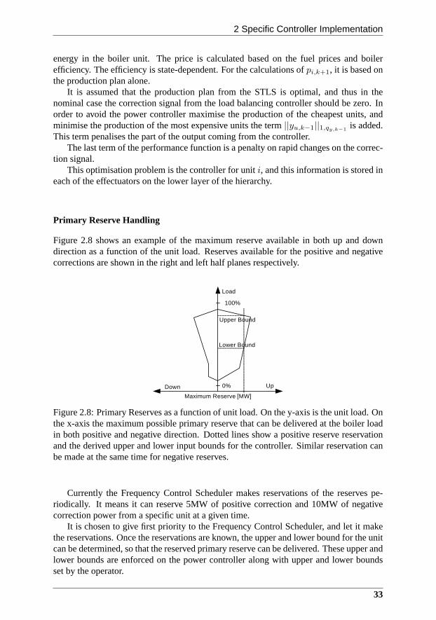
2 Specific Controller Implementation
energy in the boiler unit. The price is calculated based on the fuel prices and boilerefficiency. The efficiency is state-dependent. For the calculations ofpi,k+1, it is based onthe production plan alone.
It is assumed that the production plan from the STLS is optimal, and thus in thenominal case the correction signal from the load balancing controller should be zero. Inorder to avoid the power controller maximise the productionof the cheapest units, andminimise the production of the most expensive units the term||yu,k−1||1,qy,k−1
is added.This term penalises the part of the output coming from the controller.
The last term of the performance function is a penalty on rapid changes on the correc-tion signal.
This optimisation problem is the controller for uniti, and this information is stored ineach of the effectuators on the lower layer of the hierarchy.
Primary Reserve Handling
Figure 2.8 shows an example of the maximum reserve availablein both up and downdirection as a function of the unit load. Reserves availablefor the positive and negativecorrections are shown in the right and left half planes respectively.
Load
Maximum Reserve [MW]
0%
100%
UpDown
Lower Bound
Upper Bound
Figure 2.8: Primary Reserves as a function of unit load. On the y-axis is the unit load. Onthe x-axis the maximum possible primary reserve that can be delivered at the boiler loadin both positive and negative direction. Dotted lines show apositive reserve reservationand the derived upper and lower input bounds for the controller. Similar reservation canbe made at the same time for negative reserves.
Currently the Frequency Control Scheduler makes reservations of the reserves pe-riodically. It means it can reserve 5MW of positive correction and 10MW of negativecorrection power from a specific unit at a given time.
It is chosen to give first priority to the Frequency Control Scheduler, and let it makethe reservations. Once the reservations are known, the upper and lower bound for the unitcan be determined, so that the reserved primary reserve can be delivered. These upper andlower bounds are enforced on the power controller along withupper and lower boundsset by the operator.
33
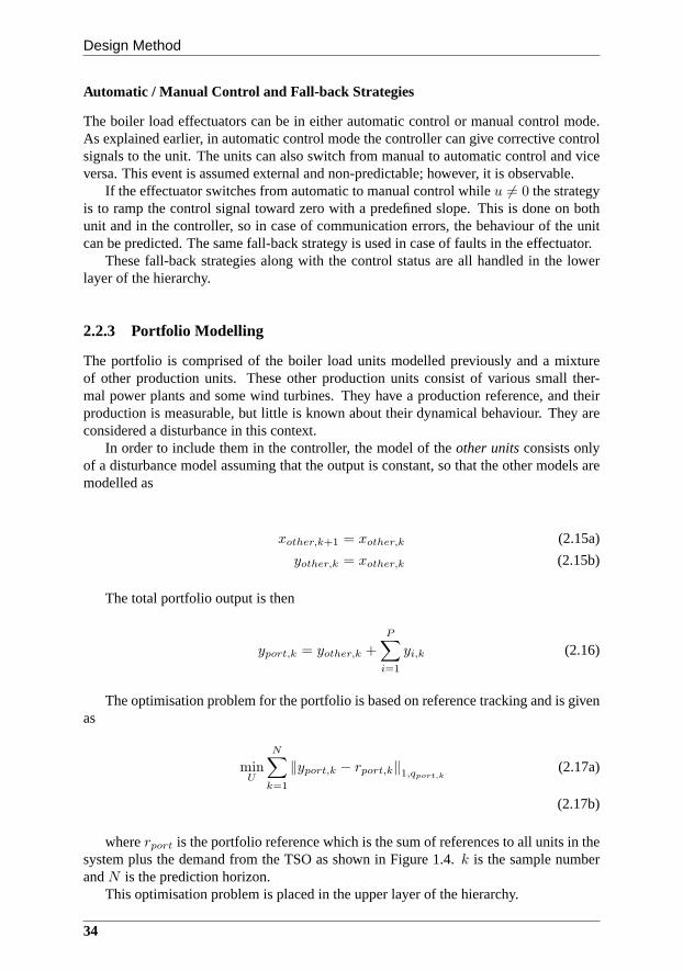
Design Method
Automatic / Manual Control and Fall-back Strategies
The boiler load effectuators can be in either automatic control or manual control mode.As explained earlier, in automatic control mode the controller can give corrective controlsignals to the unit. The units can also switch from manual to automatic control and viceversa. This event is assumed external and non-predictable;however, it is observable.
If the effectuator switches from automatic to manual control while u 6= 0 the strategyis to ramp the control signal toward zero with a predefined slope. This is done on bothunit and in the controller, so in case of communication errors, the behaviour of the unitcan be predicted. The same fall-back strategy is used in caseof faults in the effectuator.
These fall-back strategies along with the control status are all handled in the lowerlayer of the hierarchy.
2.2.3 Portfolio Modelling
The portfolio is comprised of the boiler load units modelledpreviously and a mixtureof other production units. These other production units consist of various small ther-mal power plants and some wind turbines. They have a production reference, and theirproduction is measurable, but little is known about their dynamical behaviour. They areconsidered a disturbance in this context.
In order to include them in the controller, the model of theother unitsconsists onlyof a disturbance model assuming that the output is constant,so that the other models aremodelled as
xother,k+1 = xother,k (2.15a)
yother,k = xother,k (2.15b)
The total portfolio output is then
yport,k = yother,k +
P∑
i=1
yi,k (2.16)
The optimisation problem for the portfolio is based on reference tracking and is givenas
minU
N∑
k=1
‖yport,k − rport,k‖1,qport,k(2.17a)
(2.17b)
whererport is the portfolio reference which is the sum of references to all units in thesystem plus the demand from the TSO as shown in Figure 1.4.k is the sample numberandN is the prediction horizon.
This optimisation problem is placed in the upper layer of thehierarchy.
34
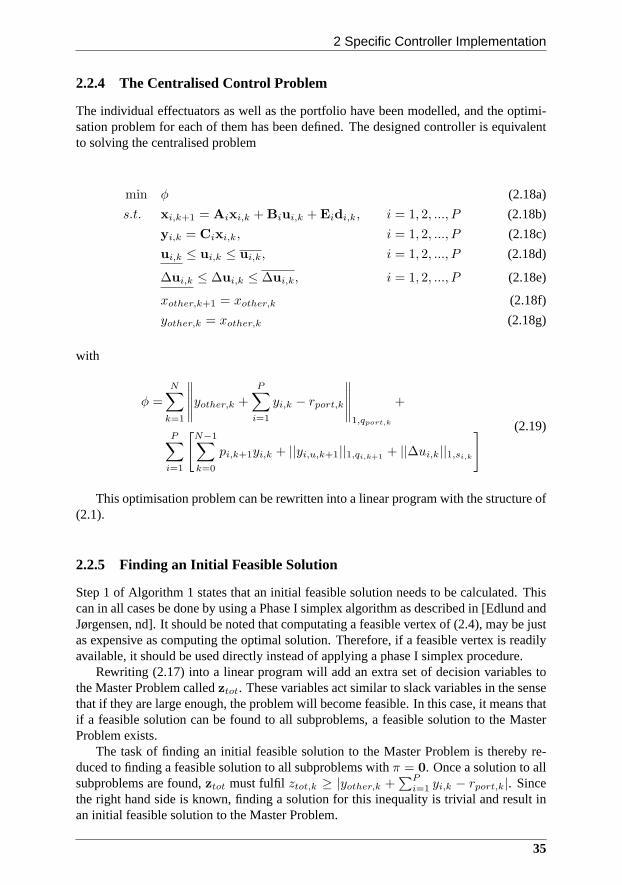
2 Specific Controller Implementation
2.2.4 The Centralised Control Problem
The individual effectuators as well as the portfolio have been modelled, and the optimi-sation problem for each of them has been defined. The designedcontroller is equivalentto solving the centralised problem
min φ (2.18a)
s.t. xi,k+1 = Aixi,k + Biui,k + Eidi,k, i = 1, 2, ..., P (2.18b)
yi,k = Cixi,k, i = 1, 2, ..., P (2.18c)
ui,k ≤ ui,k ≤ ui,k, i = 1, 2, ..., P (2.18d)
∆ui,k ≤ ∆ui,k ≤ ∆ui,k, i = 1, 2, ..., P (2.18e)
xother,k+1 = xother,k (2.18f)
yother,k = xother,k (2.18g)
with
φ =N
∑
k=1
∥
∥
∥
∥
∥
yother,k +P
∑
i=1
yi,k − rport,k
∥
∥
∥
∥
∥
1,qport,k
+
P∑
i=1
[
N−1∑
k=0
pi,k+1yi,k + ||yi,u,k+1||1,qi,k+1+ ||∆ui,k||1,si,k
]
(2.19)
This optimisation problem can be rewritten into a linear program with the structure of(2.1).
2.2.5 Finding an Initial Feasible Solution
Step 1 of Algorithm 1 states that an initial feasible solution needs to be calculated. Thiscan in all cases be done by using a Phase I simplex algorithm asdescribed in [Edlund andJørgensen, nd]. It should be noted that computating a feasible vertex of (2.4), may be justas expensive as computing the optimal solution. Therefore,if a feasible vertex is readilyavailable, it should be used directly instead of applying a phase I simplex procedure.
Rewriting (2.17) into a linear program will add an extra set of decision variables tothe Master Problem calledztot. These variables act similar to slack variables in the sensethat if they are large enough, the problem will become feasible. In this case, it means thatif a feasible solution can be found to all subproblems, a feasible solution to the MasterProblem exists.
The task of finding an initial feasible solution to the MasterProblem is thereby re-duced to finding a feasible solution to all subproblems withπ = 0. Once a solution to allsubproblems are found,ztot must fulfil ztot,k ≥ |yother,k +
∑Pi=1 yi,k − rport,k|. Since
the right hand side is known, finding a solution for this inequality is trivial and result inan initial feasible solution to the Master Problem.
35
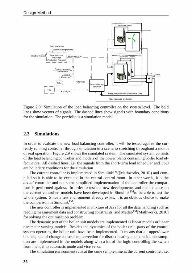
Design Method
TSO
Short-term load
scheduler
(Production Planning)
+
Production plan
Total measured production
Load balancing
controller
+
AGC signal
Filter
Expected
Response
Manual Control
Automatic Control
Measured production of individual units
Sold production
Weather forecast
District heating forecast
+Frequency control
contribution
Reference
Noise
Figure 2.9: Simulation of the load balancing controller on the system level. The boldlines show vectors of signals. The dashed lines show signalswith boundary conditionsfor the simulation. The portfolio is a simulation model.
2.3 Simulations
In order to evaluate the new load balancing controller, it will be tested against the cur-rently running controller through simulation in a scenariostretching throughout a monthof real operation. Figure 2.9 shows the simulated system. The simulated system consistsof the load balancing controller and models of the power plants containing boiler load ef-fectuators. All dashed lines, i.e. the signals from the short-term load scheduler and TSOare boundary conditions for the simulation.
The current controller is implemented in SimulinkTM([Mathworks, 2010]) and com-piled so it is able to be executed in the central control room.In other words, it is theactual controller and not some simplified implementation of the controller the compar-ison is performed against. In order to test the new developments and maintenance onthe current controller, models have been developed in SimulinkTM to be able to test thewhole system. Since a test environment already exists, it isan obvious choice to makethe comparison in SimulinkTM .
The new controller is implemented in mixture of Java for all the data handling such asreading measurement data and constructing constraints, and MatlabTM [Mathworks, 2010]for solving the optimisation problem.
The dynamic part of the boiler unit models are implemented aslinear models or linearparameter varying models. Besides the dynamics of the boiler unit, parts of the controlsystem operating the boiler unit have been implemented. It means that all upper/lowerbounds, rate of change constraints, correction for district heating and parasitic consump-tion are implemented in the models along with a lot of the logic controlling the switchfrom manual to automatic mode and vice versa.
The simulation environment runs at the same sample time as the current controller, i.e.
36
3 Simulations
0.5s, and since the sample rate of the newly developed controller is 5s, a ZOH approachwill be taken. The data is saved with a 5s sample time for both controllers for analysispurposes.
Simulations cover 25-hour sequences start from 23:00 to midnight the following day.In the analysis section, the first hour is discarded, so the analysis covers 24-hour se-quences from midnight to midnight. The first hour is used to avoid start-up and settlingissues influencing the analysis, allowing to string together several sequences for moreextensive analysis.
In this thesis only the main results from a noisy scenario aretreated for full details,see [Edlund et al., nd]. For each boiler unit the input and output sample sequences of theoriginal measured scenario are known. One can thus estimatea noise sequence for thescenario as
yn = ymeas − ysim (2.20)
This noise is applied to the output of the model of the boiler unit. Since the noise isgenerated based on closed loop measurements, it is likely filtered by the controller in theloop rather than white noise.
This noise generation is chosen, so that the simulation scenario resembles the actualscenario as closely as possible including failures. The measurements from the units mod-elled as the portfolio are applied directly to the simulation without filtering.
The analysed scenario contains three entities. There are the measurements from theactual operation, a simulation of the current controller and a simulation of the new con-troller.
For the simulations standard deviation and mean error are used as quantitative mea-surements for the evaluation. Figure 2.10 shows the mean error
µ =1
Ns
Ns∑
k=1
yport,k − rport,k (2.21)
with Ns being the number of samples in the simulation. Figure 2.11 shows the standarddeviation
σ =
√
√
√
√
1
Ns
Ns∑
k=1
((yport,k − rport,k)− µ)2 (2.22)
on a daily basis. Analysis shows that the constraints from primary reserves limit thecontroller in periods.
The standard deviation on the new controller is higher than the current controller. Asignificant change in the current and the new controller is that the new controller adheresto fulfilling the primary reserve reservations at all times.This adds an extra constraintto the controller which is active for longer periods and thisdegrades the performance ofthe new controller. A comparison of of the new controller with and without the primaryreserve constraint on a noise-free scenario is found in [Edlund et al., nd]. Both are sig-nificantly higher than the measurement data which are likelyto be caused by the noisegeneration scheme as shown in Figure 2.11. The trends in standard deviation is the samefor both controllers and measurement data. As seen in the noise-free scenario, the currenthas a slightly better performance than the proposed.
37
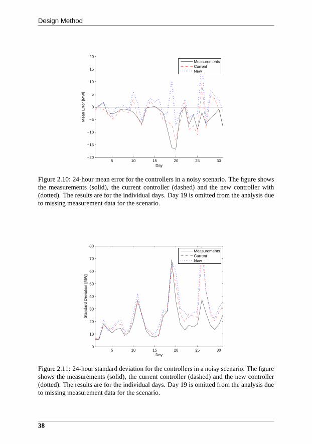
Design Method
5 10 15 20 25 30−20
−15
−10
−5
0
5
10
15
20
Day
Mea
n E
rror
[MW
]
MeasurementsCurrentNew
Figure 2.10: 24-hour mean error for the controllers in a noisy scenario. The figure showsthe measurements (solid), the current controller (dashed)and the new controller with(dotted). The results are for the individual days. Day 19 is omitted from the analysis dueto missing measurement data for the scenario.
5 10 15 20 25 300
10
20
30
40
50
60
70
80
Day
Sta
ndar
d D
evia
tion
[MW
]
MeasurementsCurrentNew
Figure 2.11: 24-hour standard deviation for the controllers in a noisy scenario. The figureshows the measurements (solid), the current controller (dashed) and the new controller(dotted). The results are for the individual days. Day 19 is omitted from the analysis dueto missing measurement data for the scenario.
38

4 Fulfilling the Design Criteria
The mean error is larger in the noisy scenario compared to thenoise-free. Thoughnot consistently lower, the average shown in Table 2.1 showsthat the new controller is anorder of magnitude closer to zero mean error compared to the current controller.
σ µMeasurements 17.74 -3.27Current 23.11 -2.78New 25.72 0.29
Table 2.1: Standard deviation and mean throughout the wholemonth of simulation. Mea-surements are the measured values with the controller running at that time. Current is asimulation with the current controller and new is the simulation with the new controller.
Figure 2.12 shows the price difference between the two controllers. Analysing theprice shows that on most days the new controller performs better. On day 20, the primaryreserves limit the controller, so that a large deviation occurs over a long period of timewhich is detrimental for the earnings of the controller. On average the difference is 240eper day, which means an earning of almost 90,000eper year.
5 10 15 20 25 30−6000
−4000
−2000
0
2000
4000
6000
Day
Diff
eren
ce in
eur
os
Figure 2.12: Price difference between the current controller and the new controller. Pos-itive difference means that the new controller is cheaper (earns more money for DONGEnergy).
2.4 Fulfilling the Design Criteria
Three design criteria has been established which the new controller needs to meet in orderto fulfil the predicted demands from such a controller.
Scalability Through the application of Dantzig-Wolfe decomposition, it is shownexperimentally in [Edlund and Jørgensen, nd] that the computational complexity
39

Design Method
of the controller grows almost linearly with the the number of effectuators whilestill converging to the same optimum as the centralised solution. This is a signifi-cant improvement in lowering the computationally complexity over the centralisedsolution. It is also shown that already at 2-3 effectuators,the Dantzig-Wolfe de-composition is faster than the centralised solution. Furthermore, it is possible todistribute the optimisation problem among multiple processors, giving an advan-tage which exploits the trends toward computers with multiple processors.
Flexibility The design method fulfils the objective of flexibility through an object-oriented design with data encapsulation and clear interfaces. It ensures that thecontroller is easily maintainable in case of updates of the controller such as addingand removing effectuators.
Performance The design method itself does not ensure that the performance cri-terion is met, so that a controller design with the developedmethod performs aswell as the current controller. However, the developed method ensures that if anℓ1-norm based MPC can be constructed to fulfil the performance criterion, the designhierarchical design will also fulfil the criterion. In Section 2.3 as well as [Edlundet al., 2008, nd], simulations show that anℓ1-norm based MPC can be constructed,which improves the performance in terms of standard deviation and mean value, aswell as improve the economic performance by a better distribution of the controlactions.
The scalability and flexibility criteria have both been treated and fulfilled by the designmethod, while the performance criterion is dependent on thespecific implementation.The design method has been utilised for controller synthesis for the current power plantportfolio and the resulting controller fulfills the performance criterion. Thus, all criteriaestablished in the hypothesis can be fulfilled by the design method.
40
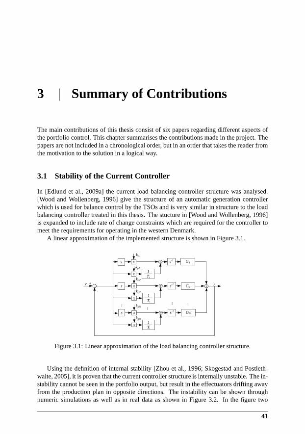
3 Summary of Contributions
The main contributions of this thesis consist of six papers regarding different aspects ofthe portfolio control. This chapter summarises the contributions made in the project. Thepapers are not included in a chronological order, but in an order that takes the reader fromthe motivation to the solution in a logical way.
3.1 Stability of the Current Controller
In [Edlund et al., 2009a] the current load balancing controller structure was analysed.[Wood and Wollenberg, 1996] give the structure of an automatic generation controllerwhich is used for balance control by the TSOs and is very similar in structure to the loadbalancing controller treated in this thesis. The stucture in [Wood and Wollenberg, 1996]is expanded to include rate of change constraints which are required for the controller tomeet the requirements for operating in the western Denmark.
A linear approximation of the implemented structure is shown in Figure 3.1.
-
++
G1
G2
GN
s x
x1Ti
kp1
kp1
s-1
s x
x
s-1
1Ti
s x
x1Ti
s-1
kp2
kp2
kpN
kpN
+
+
+
y
......
.....
.
r
Figure 3.1: Linear approximation of the load balancing controller structure.
Using the definition of internal stability [Zhou et al., 1996; Skogestad and Postleth-waite, 2005], it is proven that the current controller structure is internally unstable. The in-stability cannot be seen in the portfolio output, but resultin the effectuators drifting awayfrom the production plan in opposite directions. The instability can be shown throughnumeric simulations as well as in real data as shown in Figure3.2. In the figure two
41
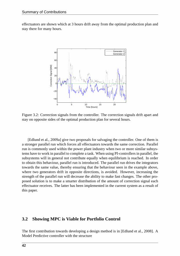
Summary of Contributions
effectuators are shown which at 3 hours drift away from the optimal production plan andstay there for many hours.
0 5 10 15 20
−40
−20
0
20
40
60
80
Time [hours]
Cor
rect
ion
Sig
nal [
MW
]
Generator 1Generator 2
Figure 3.2: Correction signals from the controller. The correction signals drift apart andstay on opposite sides of the optimal production plan for several hours.
[Edlund et al., 2009a] give two proposals for salvaging the controller. One of them isa stronger parallel run which forces all effectuators towards the same correction. Parallelrun is commonly used within the power plant industry when twoor more similar subsys-tems have to work in parallel to complete a task. When using PI-controllers in parallel, thesubsystems will in general not contribute equally when equilibrium is reached. In orderto obtain this behaviour, parallel run is introduced. The parallel run drives the integratorstowards the same value, thereby ensuring that the behaviourseen in the example above,where two generators drift in opposite directions, is avoided. However, increasing thestrength of the parallel run will decrease the ability to make fast changes. The other pro-posed solution is to make a smarter distribution of the amount of correction signal eacheffectuator receives. The latter has been implemented in the current system as a result ofthis paper.
3.2 Showing MPC is Viable for Portfolio Control
The first contribution towards developing a design method isin [Edlund et al., 2008]. AModel Predictive controller with the structure
42
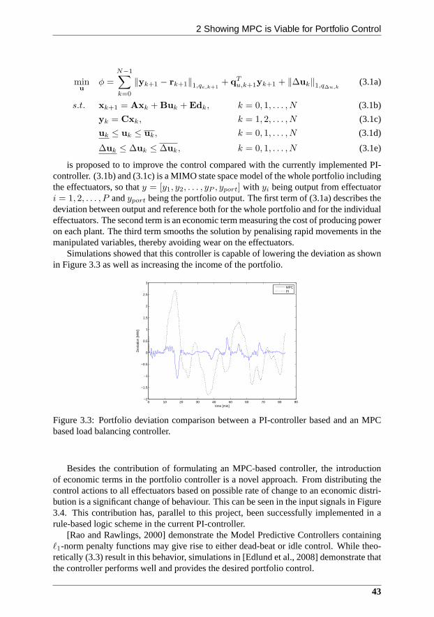
2 Showing MPC is Viable for Portfolio Control
minu
φ =
N−1∑
k=0
‖yk+1 − rk+1‖1,qe,k+1+ qT
u,k+1yk+1 + ‖∆uk‖1,q∆u,k(3.1a)
s.t. xk+1 = Axk + Buk + Edk, k = 0, 1, . . . , N (3.1b)
yk = Cxk, k = 1, 2, . . . , N (3.1c)
uk ≤ uk ≤ uk, k = 0, 1, . . . , N (3.1d)
∆uk ≤ ∆uk ≤ ∆uk, k = 0, 1, . . . , N (3.1e)
is proposed to to improve the control compared with the currently implemented PI-controller. (3.1b) and (3.1c) is a MIMO state space model of the whole portfolio includingthe effectuators, so thaty = [y1, y2, . . . , yP , yport] with yi being output from effectuatori = 1, 2, . . . , P andyport being the portfolio output. The first term of (3.1a) describes thedeviation between output and reference both for the whole portfolio and for the individualeffectuators. The second term is an economic term measuringthe cost of producing poweron each plant. The third term smooths the solution by penalising rapid movements in themanipulated variables, thereby avoiding wear on the effectuators.
Simulations showed that this controller is capable of lowering the deviation as shownin Figure 3.3 as well as increasing the income of the portfolio.
0 10 20 30 40 50 60 70 80 90−2
−1.5
−1
−0.5
0
0.5
1
1.5
2
2.5
3
time [min]
Dev
iatio
n [M
W]
MPCPI
Figure 3.3: Portfolio deviation comparison between a PI-controller based and an MPCbased load balancing controller.
Besides the contribution of formulating an MPC-based controller, the introductionof economic terms in the portfolio controller is a novel approach. From distributing thecontrol actions to all effectuators based on possible rate of change to an economic distri-bution is a significant change of behaviour. This can be seen in the input signals in Figure3.4. This contribution has, parallel to this project, been successfully implemented in arule-based logic scheme in the current PI-controller.
[Rao and Rawlings, 2000] demonstrate the Model Predictive Controllers containingℓ1-norm penalty functions may give rise to either dead-beat oridle control. While theo-retically (3.3) result in this behavior, simulations in [Edlund et al., 2008] demonstrate thatthe controller performs well and provides the desired portfolio control.
43
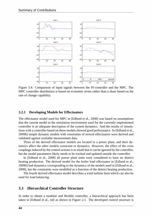
Summary of Contributions
0 20 40 60 80−20
−10
0
10
Unit 1
0 20 40 60 80−20
−10
0
10
Unit 2
0 20 40 60 80−20
−10
0
10
Unit 3
0 20 40 60 80−20
−10
0
10
Unit 4
0 20 40 60 80−20
−10
0
10
Unit 5
0 20 40 60 80−20
−10
0
10
Unit 6
PI MPC Bound
Figure 3.4: Comparison of input signals between the PI-controller and the MPC. TheMPC controller distribution is based on economic terms rather than a share based on therate of change capability.
3.2.1 Developing Models for Effectuators
The effectuator model used for MPC in [Edlund et al., 2008] was based on assumptionsthat the current model in the simulation environment used for the currently implementedcontroller is an adequate description of the system dynamics. And the results of simula-tions with a controller based on these models showed good performance. In [Edlund et al.,2009b] simple dynamic models with constraints of several effectuators were derived andvalidated against available measurement data.
Three of the derived effectuator models are located in a power plant, and their dy-namics affect the other models constraint or dynamics. However, the effect of the crosscouplings induced by the control actions is so small that it can be ignored by the controller,but the model parameters likely needs to be tracked and updated outside the controller.
In [Edlund et al., 2008] all power plant units were considered to have no districtheating production. The derived model for the boiler load effectuator in [Edlund et al.,2009b] had dynamics corresponding to the dynamics of the models used in [Edlund et al.,2008], but the constraints were modelled as a function of thedistrict heating production.
The fourth derived effectuator model describes a wind turbine farm which can also beused for load balancing.
3.3 Hierarchical Controller Structure
In order to obtain a modular and flexible controller, a hierarchical approach has beentaken in [Edlund et al., nd] as shown in Figure 2.1. The developed control structure is
44
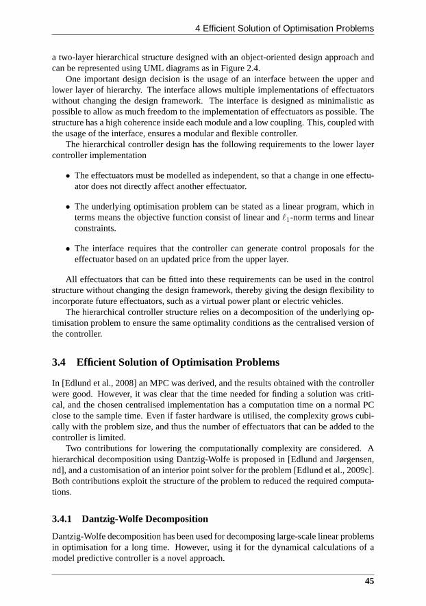
4 Efficient Solution of Optimisation Problems
a two-layer hierarchical structure designed with an object-oriented design approach andcan be represented using UML diagrams as in Figure 2.4.
One important design decision is the usage of an interface between the upper andlower layer of hierarchy. The interface allows multiple implementations of effectuatorswithout changing the design framework. The interface is designed as minimalistic aspossible to allow as much freedom to the implementation of effectuators as possible. Thestructure has a high coherence inside each module and a low coupling. This, coupled withthe usage of the interface, ensures a modular and flexible controller.
The hierarchical controller design has the following requirements to the lower layercontroller implementation
• The effectuators must be modelled as independent, so that a change in one effectu-ator does not directly affect another effectuator.
• The underlying optimisation problem can be stated as a linear program, which interms means the objective function consist of linear andℓ1-norm terms and linearconstraints.
• The interface requires that the controller can generate control proposals for theeffectuator based on an updated price from the upper layer.
All effectuators that can be fitted into these requirements can be used in the controlstructure without changing the design framework, thereby giving the design flexibility toincorporate future effectuators, such as a virtual power plant or electric vehicles.
The hierarchical controller structure relies on a decomposition of the underlying op-timisation problem to ensure the same optimality conditions as the centralised version ofthe controller.
3.4 Efficient Solution of Optimisation Problems
In [Edlund et al., 2008] an MPC was derived, and the results obtained with the controllerwere good. However, it was clear that the time needed for finding a solution was criti-cal, and the chosen centralised implementation has a computation time on a normal PCclose to the sample time. Even if faster hardware is utilised, the complexity grows cubi-cally with the problem size, and thus the number of effectuators that can be added to thecontroller is limited.
Two contributions for lowering the computationally complexity are considered. Ahierarchical decomposition using Dantzig-Wolfe is proposed in [Edlund and Jørgensen,nd], and a customisation of an interior point solver for the problem [Edlund et al., 2009c].Both contributions exploit the structure of the problem to reduced the required computa-tions.
3.4.1 Dantzig-Wolfe Decomposition
Dantzig-Wolfe decomposition has been used for decomposinglarge-scale linear problemsin optimisation for a long time. However, using it for the dynamical calculations of amodel predictive controller is a novel approach.
45

Summary of Contributions
The benefits of using Dantzig-Wolfe decomposition are that the hierarchical structureis possible to implement with a clear interface with a small level of communication. Be-sides the clear interface design, it also makes it possible to spread the optimisation overmultiple computers connected by a network, without much overhead.
Dantzig-Wolfe decomposition also ensures better scalability. Scalability in computa-tionally complexity is shown in Figure 3.5.
103 50
10−1
100
101
# of effectuators
Ave
rage
exe
cutio
n tim
e pe
r sa
mpl
e [s
]
Centralised
0.007*x3.25
Dantzig−Wolfe
0.05*x1.1
Parallel Dantzig−Wolfe0.02*x
Figure 3.5: Computation time as a function of the effectuators in the optimisation.
Computation time grows almost linearly with the number of effectuators compared tothe cubic growth of a centralised solution. This coupled with the algorithm being fasterwith a small number of effectuators makes MPC a viable controller scheme for the loadbalancing controller.
Theoretically, the Dantzig-Wolfe decomposition converges very slowly, the test prob-lem in [Edlund and Jørgensen, nd], and the simulation on a realistic scenario [Edlundet al., nd] shows good convergence in practice.
3.4.2 Customising an Interior Point Method
The other contribution toward increasing the efficiency of the optimisation algorithm wascustomising an interior point method which is reported in [Edlund et al., 2009c]. Theinterior point method is tailored to solve the local optimisation related to one of the boilerload effectuators. However, many of the techniques appliedcan be reused in MPC appli-cations.
46
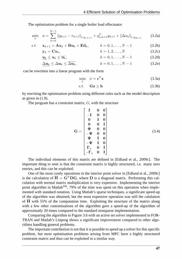
4 Efficient Solution of Optimisation Problems
The optimisation problem for a single boiler load effectuator
minu
φ =
N−1∑
k=0
‖yk+1 − rk+1‖1,qe,k+1+ qT
u,k+1yk+1 + ‖∆uk‖1,q∆u,k(3.2a)
s.t. xk+1 = Axk + Buk + Edk, k = 0, 1, . . . , N − 1 (3.2b)
yk = Cxk, k = 1, 2, . . . , N (3.2c)
uk ≤ uk ≤ uk, k = 0, 1, . . . , N − 1 (3.2d)
∆uk ≤ ∆uk ≤ ∆uk, k = 0, 1, . . . , N − 1 (3.2e)
can be rewritten into a linear program with the form
minx
φ = cT z (3.3a)
s.t. Gz ≥ h (3.3b)
by rewriting the optimisation problem using different rules such as the model descriptionas given in (1.9).
The program has a constraint matrix,G, with the structure
G =
I 0 0
−I 0 0
0 I 0
0 0 I
Ψ 0 0
−Ψ 0 0
Ψ I 0
−Ψ I 0
Γu 0 I
−Γu 0 I
(3.4)
The individual elements of this matrix are defined in [Edlundet al., 2009c]. Theimportant thing to note is that the constraint matrix is highly structured, i.e. many zeroentries, and this can be exploited.
One of the most costly operations in the interior point solver in [Edlund et al., 2009c]is the calculation ofH = GT DG, whereD is a diagonal matrix. Performing this cal-culation with normal matrix multiplication is very expensive. Implementing the interiorpoint algorithm in MatlabTM , 79% of the time was spent on this operation when imple-mented with standard notation. Using Matlab’s sparse techniques, a significant speed-upof the algorithm was obtained, but the most expensive operation was still the calulationof H with 55% of the computation time. Exploiting the structure of the matrix alongwith a few other customisations of the algorithm gave a speed-up of the algorithm ofapproximatly 20 times compared to the standard nonsparse implementation.
Comparing the algorithm in Figure 3.6 with an active set solver implemented in FOR-TRAN and Matlab’s Linprog shows a significant improvement compared to other algo-rithms handling general problems.
The important contribution is not that it is possible to speed up a solver for this specificproblem, but most optimisation problems arising from MPC have a highly structuredconstraint matrix and thus can be exploited in a similar way.
47

Summary of Contributions
Figure 3.6: CPU times for the different LP algorithms.
Dantzig-Wolfe Decomposition relies on the subproblems to generate solutions in avertex of the feasible area. In the rare case that a solution to the subproblem exists on anedge of the feasible area, the interior point method might not converge to a vertex. Sousing the customised interior point method to efficiently solve the subproblems generatedby Dantzig-Wolfe decomposition could lead to a Dantzig-Wolfe algorithm which will notconverge to an optimum. In practice this has not proved to be aproblem.
3.5 Implementation and Benchmarking of the Controller
Throughout the project, implementations of the controllerhave been made. The firstimplementation is reported in [Edlund et al., 2008] with thepurpose of showing thatMPC is a viable option for a control scheme as described in Section 3.2.
In [Edlund et al., nd] the design method was used to synthesisof a controller for usein the current system. The performance of the controller designed with the developedmethod was compared based on three factors; mean error, standard deviation and price.The comparison was performed through a simulation in a scenario based on data from amonth of actual operation.
The new method incorporates a method to ensure that the load balancing controllerdoes not violate the primary reserve constraints, something that has not been handledpreviously.
Table 3.1 shows a comparison of the new controller compared with the current im-plementation. There are three tested entities; there are the measurements from the actualoperation, a simulation of the currently implemented controller and a simulation of theproposed new controller. The new controller includes constraints to ensure that primaryreserves are maintained. For comparison purposes the new controller has been simulatedwithout this constraint as well.
In both the noise-free and the noisy scenario, the new controller performs close to butslightly worse than the current controller. The hypothesiswas that it was caused by theconstraints enforced by the primary reserves. The comparison with the new controller
48
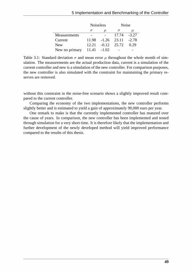
5 Implementation and Benchmarking of the Controller
Noiseless Noiseσ µ σ µ
Measurements - - 17.74 -3.27Current 11.98 -1.26 23.11 -2.78New 12.21 -0.12 25.72 0.29New no primary 11.41 -1.02 - -
Table 3.1: Standard deviationσ and mean errorµ throughout the whole month of sim-ulation. The measurements are the actual production data, current is a simulation of thecurrent controller and new is a simulation of the new controller. For comparison purposes,the new controller is also simulated with the constraint formaintaining the primary re-serves are removed.
without this constraint in the noise-free scenario shows a slightly improved result com-pared to the current controller.
Comparing the economy of the two implementations, the new controller performsslightly better and is estimated to yield a gain of approximately 90,000 euro per year.
One remark to make is that the currently implemented controller has matured overthe cause of years. In comparison, the new controller has been implemented and testedthrough simulation for a very short time. It is therefore likely that the implementation andfurther development of the newly developed method will yield improved performancecompared to the results of this thesis.
49

4 Conclusion
When the project started, the scalability of the controller was a feature which might be re-quired at some point in the future, but the main focus was the performance improvementon the current portfolio. During the course of the project the drive towards more sustain-able energy production has changed the energy system, so that scalability has becomeabsolutely crucial to the controller design. An example of this change is the rapid devel-opment of virtual power plants and thereby a potential increase in number of effectuatorsin control in the very near future.
The power system is very complex, and with the increasing number of effectuatorscomplexity will increase even more. One of the aims in this thesis has been to develop adesign method which is clear and relatively simple to ensurethat it can be implementedin the production at some point. This includes a very high level of abstraction.
To test whether it was possible to develop a design method, a hypothesis was for-mulated stating that it is possible to develop a controller design method which leads tosynthesis of a controller which fulfils the criteria of scalability, flexibility and perfor-mance.
A design method has been developed which results in synthesis of a controller with anobject-oriented structure with clear interfaces, thus ensuring theflexibility of the controlstructure. The modular design ensures that the controller is easily maintainable in case ofupdates of the controller such as adding and removing effectuators. The use of interfacesin the design offers flexibility in the implementation of thecontrol formulation for theindividual effectuator.
By using Dantzig-Wolfe decomposition, a computational efficient solution can be ob-tained which grows linearly with the number of effectuatorsin control. Furthermore,decomposition allows distribution of the optimisation among several computers, thus im-proving thescalability significantly compared to a centralised solution. A customisedinterior point solver can be utilised to efficiently solve the smaller distributed problems inthe hierarchical structure.
Using the design method for synthesis of a controller for thecurrent portfolio, thesimulatedperformanceis comparable with the simulated performance of the currentlyimplemented PI-controller structure.
The developed design method fulfils all three criteria of thehypothesis, therefore thehypothesis is accepted.
The contributions of the work consist of six papers describing different aspects ofportfolio control as well as the development of the method. In summary, the contributionscan be listed as:
51
Conclusion
• Analysis of the current controller structure, based on the structure used in literature.The structure was proven unstable. There are, however, methods for stabilising thecontroller. [Edlund et al., 2009a]
• Formulation of the load balancing problem as a model predictive controller, andshowing that the current state of the art within load balancing control can be im-proved by introducing Model predictive control theory. [Edlund et al., 2008]
• Developing a method for synthesising a load balancing controller with a modulardesign and clear interfaces using model predictive control. The design is a two-layer hierarchical structure which has a performance equalto a centralised solu-tion. The design method requires that the underlying optimisation problem can beformulated as a linear program. [Edlund et al., nd]
• Customisation of a general interior point method to exploitthe structure of thespecific problem in order to speed up the optimisation, by exploiting the structureof the problem. [Edlund et al., 2009c]
• Introduction of Dantzig-Wolfe decomposition for the dynamic calculations of MPCfor use in portfolio load balancing control. The result is anindependent problemscorresponding to the physical subsystems. [Edlund and Jørgensen, nd]
• Implementation of the method on the existing portfolio and compared the perfor-mance with the current controller through simulations. Thecomparison showedthat the developed method has potential to improve performance in the existingportfolio. [Edlund et al., nd]
• Developing a method for ensuring that primary reserves are maintained when theload balancing controller performs internal balance control. It is a prerequisite thatthe reserves are available from the beginning. [Edlund et al., nd]
4.1 Future Work
The design method for a load balancing controller presentedin this thesis fulfils the cri-teria to be able to accept the hypothesis. There are two pathstwo be followed after thisproject is finished. One path is the industrial implementation maturing and implementa-tion of the controller in a suitable application. The other is further development of thecontroller design to remove some of the limitations the current design method imply.
• A design method and a prototype of an implementation has beenprovided in thisthesis, but in order to implement and use the controller in operation it must bematured and implemented to fit in the platform of the control system. Further-more, only the controller core has been developed, in order to have a fully fledgedcontroller suitable for operation it has to be expanded to include elements such ascommunication and operator interface.
• The design method enables inclusion of new effectuators in the portfolio in a rela-tivity straight forward manner. Identification and construction of new effectuatorsare not directly related successors of this thesis. But the framework for includingthem in balancing control is now established and ready for this task.
52

1 Future Work
• The proposed controller design relies on one Kalman filter for state estimation ofthe whole system. The complexity of the matrix multiplications grows cubicallywith the problem size. This could prove to be a limiting factor for the scalability inthe proposed control design. However, the computation timespent on the Kalmanfilter in the implementation is insignificant compared to thecomputation time spentby the controller. A logical extension of the design method would be to include adistributed state estimator as well. Distributed state estimation has already beentreated in [Alriksson and Rantzer, 2006; Farina et al., 2009] among others, butneeds to be incorporated in the method. Incorporating distributed estimation intothe method would ensure that the estimator would fit into the framework, therebyensuring that each of the modules for the individual effectuators contain all infor-mation needed to add the effectuator to the control.
• Currently, the design method requires that the controller can be stated as a linearprogram to be able to perform the optimisation. Expansion ofthe controller de-sign is a topic for further research. Inclusion of nonlinearities in both performancefunction and constraint is the ultimate goal, but the next logical step is to includequadratic terms in the performance function since it would enable the frameworkto handle the most common MPC formulation.
• Simulations show that the discrete events generated by effectuators being added toor removed from the controller do not induce large deviations or cause instabili-ties. However, there is not established firm theoretical guarantees that these eventswill not destabilise the system. A theoretical foundation ensuring these propertieswould be a clear enhancement of the robustness of controller.
• Currently, the events of adding and removing effectuators are generated externally.Expanding the controller to predict when it is safe and/or optimal to add and removeeffectators is another topic of future research closely related to the stability analysisabove. This topic can be generalised to the controller beingable to handle discreteevents, and thus removing the limitation that the effectuators must be continuous tobe included in the control. This would significantly expand the types of effectuatorsthat can be handled by the controller.
53


References
L. Acar. Boundaries of the Receding Horizon Control for Interconnected Systems.Jour-nal of Optimization Theory and Applications, 84(2):251–271, 1995.
B. M. Akesson, J. B. Jørgensen, N. K. Poulsen, and S. B. Jørgensen.A GeneralizedAutocovariance Least-Squares Method for Covariance Estimation. Proceedings of the2007 American Control Conference, New York, USA, pages 3713–3714, 2007.
C. Albenesi, M. Bossi, L. Magni, J. Paderno, Pretolani, P. Kuehl, and M. Diehl. Optimiza-tion of the Start-up Procedure of a Combined Cycle Power Plant. Proceedings of the45th IEEE Conference on Decision and Control, San Diego, USA, pages 1840–1845,2006.
F. Allgower, T. A. Badgwell, J. B. Rawlings, and S. J. Wright. Nonlinear model pre-dictive control. InPerspectives in Control. Plenary Lectures and Mini-Courses at the5th European Control Conference ECC’99, pages 391–449. Springer-Verlag, London,1999.
J. Allwright and G. Papavasiliou. On Linear Programming andRobust Model-PredictiveControl Using Impulse-Responses.Systems & Control Letters, 18(2):159–164, 1992.
P. Alriksson and A. Rantzer. Distributed Kalman Filtering Using Weighted Averaging. InProceedings of the 17th International Symposium on Mathematical Theory of Networksand Systems, Kyoto, Japan, Kyoto, Japan, 2006.
K. Aoki, T. Satoh, M. Itoh, T. Ichimori, and K. Masegi. Unit Commitment in a Large-Scale Power System including Fuel Constrained Thermal and Pumped-Storage Hydro.IEEE Transactions on Power Systems, 2(4):1077–1084, 1987.
K. J. Astrom and T. Hagglund. Advanced PID Control. ISA - Instrumention, Systemsand Automation Society, 2006. ISBN 1-556-17942-1.
A. K. Ayuob and A. D. Patton. Optimal thermal generating unitcommitment. IEEETransactions on Power Apparatus and Systems, 90(4):1752–1756, 1971.
M. Azzam and Y. S. Mohamed. Robust controller design for automatic generation controlbased on Q-parameterization.Energy Conversion and Management, 1(43):1663–1673,2002.
B. H. Bakken and O. S. Grande. Automatic Generation Control in a Deregulated PowerSystem.IEEE Transactions on Power Systems, 13(4):1401–1406, 1998.
55
REFERENCES
H. Banakar, C. Luo, and B. T. Ooi. Impacts of Wind Power Minute-to-Minute Variationson Power System Operation.IEEE Transactions on Power Systems, 23(1):150–160,2008.
J. E. Beasley.Modern heuristic techniques for combinatorial problems. John Wiley &Sons, Inc., New York, NY, USA, 1993. ISBN 0-470-22079-1.
A. Bemporad, M. Morari, V. Dua, and E. N. Pistikopoulos. The explicit linear quadraticregulator for constrained systems.Automatica, 38(1):3–20, 2002.
J. F. Benders. Partitioning procedures for solving mixed-variables programming prob-lems.Numer. Math., 4(3):238–252, 1962.
J. D. Bendtsen and K. Trangbæk. Stable controller reconfiguration through terminal con-nections A practical example.2009 IEEE International Conference on Control andAutomation, Christchurch, New Zealand, pages 2037–2042, 2009.
C. Bjerge and J. R. Kristoffersen. Run an offshore wind farm like a power plant.VGBPowertech, 87(4):63–66, 2007.
M. Blanke, M. Kinnaert, J. Lunze, M. Staroswiecki, and J. Schroder. Diagnosis andFault-Tolerant Control. Springer-Verlag New York, Inc., 2006. ISBN 3-540-01056-4.
S. Boyd and L. Vandenberghe.Convex Optimization. Cambridge University Press, Cam-bridge, UK, 2004. ISBN 0-521-83378-7.
T. S. Chang and D. E. Seborg. A linear programming approach tomultivariable feedbackcontrol with inequality constraints.International Journal of Control, 37(3):583–597,1983.
L. Chen, J. Zhong, and D. Gan. Optimal Automatic Generation Control (AGC) Dis-patching and Its Control Performance Analysis for the Distribution Systems with DGs.Power Engineering Society General Meeting, 2007, Tampa, USA, pages 1–6, 2007.
R. Cheng, J. F. Forbes, and W. S. Yip. Price-driven coordination method for solvingplant-wide MPC problems.Journal of Process Control, 17(5):429–438, 2007.
R. Cheng, J. F. Forbes, and W. S. Yip. Dantzig-Wolfe decomposition and plant-wideMPC coordination.Computers and Chemical Engineering, 32(7):1507–1522, 2008.
N. N. Chokshi and D. C. McFarlane.A Distributed Coordination Approach to Reconfig-urable Process Control. Springer-Verlag, 2008. ISBN 1-848-00059-9.
J. Czyzyk, S. Mehrotra, M. Wagner, and S. J. Wright. PCx: An Interior-Point Code forLinear Programming.Optimization Methods and Software, 11(1):397–430, 1999.
M. J. Dahl-Soerensen and B. Solberg. Pulverized Fuel Control using Biased Flow Mea-surements.Proceedings of the IFAC Symposium on Power Plants and Power SystemsControl, Tampera, Finland, 2009.
Danish Ministry of Transport and Energy. Energistrategi 2025 - Perspektiver frem mod2025. Technical report, Transport- og Energiministeriet,2005.
56
REFERENCES
G. B. Dantzig and M. N. Thapa.Linear programming 1: Introduction. Springer Verlag,1997. ISBN 0-387-94833-3.
G. B. Dantzig and M. N. Thapa.Linear Programming 2: Theory and Extensions.Springer-Verlag, 2002. ISBN 0-387-98613-8.
G. B. Dantzig and P. Wolfe. Decomposition Principle for Linear Programs.Operationsresearch, 8(1):101–111, 1960.
F. P. de Mello. Boiler models for system dynamical performance studies.IEEE Transac-tions on Power Systems, 6(1):66–74, 1991.
L. Deprugney and J.-B. Liters. New excess air controller at Le Havre Power Plant.14th Annual Joint ISA Power Industry Division and EPRI Controls and Instrumenta-tion Conference/47th Annual ISA Power Industry Symposium,Proceedings, ColoradoSprings, USA, pages 1–14, 2004.
L. Deprugney, S. Maurin, A. Girard, and H. Jestin. New advanced coordinated controllerfor once-through boiler and turbine of coal-fired power plant. 16th Annual Joint ISAPOWID/EPRI Controls and Instrumentation Conference and 49th Annual ISA PowerIndustry Division, POWID Symposium 2006, San Jose, USA, pages 36–59, 2006.
T. S. Dillon, K. W. Edwin, H. D. Kochs, and R. J. Taud. Integer Programming Approach tothe Problem of Optimal Unit Commitment with Probabilistic Reserve Determination.IEEE Transactions on Power Apparatus and Systems, PAS-97(6):2154–2166, 1978.
DONG Energy.http://www.dongenergy.dk, 2010.
J. Doyle and G. Stein. Multivariable feedback Design.IEEE Transactions on AutomaticControl, 26(1):4–16, 1981.
W. B. Dunbar. Distributed Receding Horizon Control of Dynamically Coupled NonlinearSystems.IEEE Transactions on Automatic Control, 52(7):1249–1263, 2007.
J. W. Eaton and J. B. Rawlings. Model-Predictive Control of Chemical Processes.Chem-ical Engineering Science, 47(4):705–720, 1992.
K. Edlund and J. B. Jørgensen. Dantzig-Wolfe Algorithm for Power Plant Portfolio Con-trol. Submitted for International Journal of Control, nd.
K. Edlund, J. D. Bendtsen, S. Børresen, and T. Mølbak. Introducing Model PredictiveControl for Improving Power Plant Portfolio Performance.Proceedings of the 17thIFAC World Congress, Seoul, South Korea, pages 6986–6991, 2008.
K. Edlund, J. D. Bendtsen, and P. Andersen. Structural Stability Analysis of a Rate Lim-ited Automatic Generation Control System.Proceedings of European Control Confer-ence, Budapest, Hungary, pages 4534–4539, 2009a.
K. Edlund, T. Mølbak, and J. D. Bendtsen. Simple Models for Model-based Portfo-lio Load Balancing Controller Synthesis.Proceedings of IFAC Symposium on powerplants and power systems control 2009, Tampera, Finland, 2009b.
57
REFERENCES
K. Edlund, L. E. Sokoler, and J. B. Jørgensen. A Primal-Dual Interior-Point Linear Pro-gramming Algorithm for MPC.Proceedings of 48th IEEE Conference on Decision andControl, Shanghai, China, pages 351–356, 2009c.
K. Edlund, J. D. Bendtsen, and J. B. Jørgensen. Hierarchicalmodel-based predictivecontrol of power plant portfolio.Submitted for Control Engineering Practice, nd.
M. S. Elliott and B. P. Rasmussen. Model-based predictive control of a multi-evaporatorvapor compression cooling cycle.Proceedings of the 2008 American Control Confer-ence, Seattle, USA, pages 1463–1468, 2008.
Energinet.dk. Common market regulations for electricity in Eastern and WesternDenmark. http://www.energinet.dk/en/servicemenu/Library/Rules+and+Regulations/Common+market+regulations+for+electricity+in+Eastern+and+Western+Denmark, 2010.
ENTSO-E.http://www.entsoe.eu/, 2010a.
ENTSO-E. ENTSO-E Operational handbook.http://www.entsoe.eu/index.php?id=57, 2010b.
M. Farina, G. Ferrari-Trecate, and R. Scattolini. A moving horizon scheme for distributedstate estimation.Proceedings of the 48h IEEE Conference on Decision and Control,Shanghai, China, pages 1818–1823, 2009.
R. Franke and L. Vogelbacher. Nonlinear model predictive control for cost optimal startupof steam power plants.Automatisierungstechnik, 54(12):630–637, 2006.
G. F. Franklin, J. D. Powell, and A. Emami-Naeini.Feedback control of Dynamic Systems.Prentice Hall, 4th edition, 2002. ISBN 0-130-32393-4.
J. B. Froisy. Model predictive control Building a bridge between theory and practice.Computers and Chemical Engineering, 30(10–12):1426–1435, 2006.
B. P. Gibbs, D. S. Weber, and D. W. Porter. Application of Nonlinear Model-BasedPredictive Control to Fossil Power Plants.Proceedings of the 30th IEEE Conferenceon Decision and Control, Brighton, England, pages 1850–1856, 1991.
M. S. Grewal and A. P. Andrews.Kalman Filtering Theory and Practice using Matlab.John Wiley & Sons, inc, 3rd edition, 2008. ISBN 0-471-39254-5.
V. Gunnerud, B. Foss, B. Nygreen, R. Vestb, and N. C. Walberg.Dantzig-Wolfe decom-position for real-time optimization - applied to the Troll west oil rim. Proceedingsof International Symposium on Advanced Control of ChemicalProcesses, Istanbul,Turkey, 2009.
M. F. Hassan, A. A. Abouelsoud, and H. M. Soliman. Constrained Load-frequency Con-trol. Electric Power Components and Systems, 36(3):266–279, 2008.
R. Iserman. Fault-Diagnosis Systems: An Introduction from Fault Detection to FaultTolerance. Spring-Verlag, 2005. ISBN 3-540-24112-4.
58
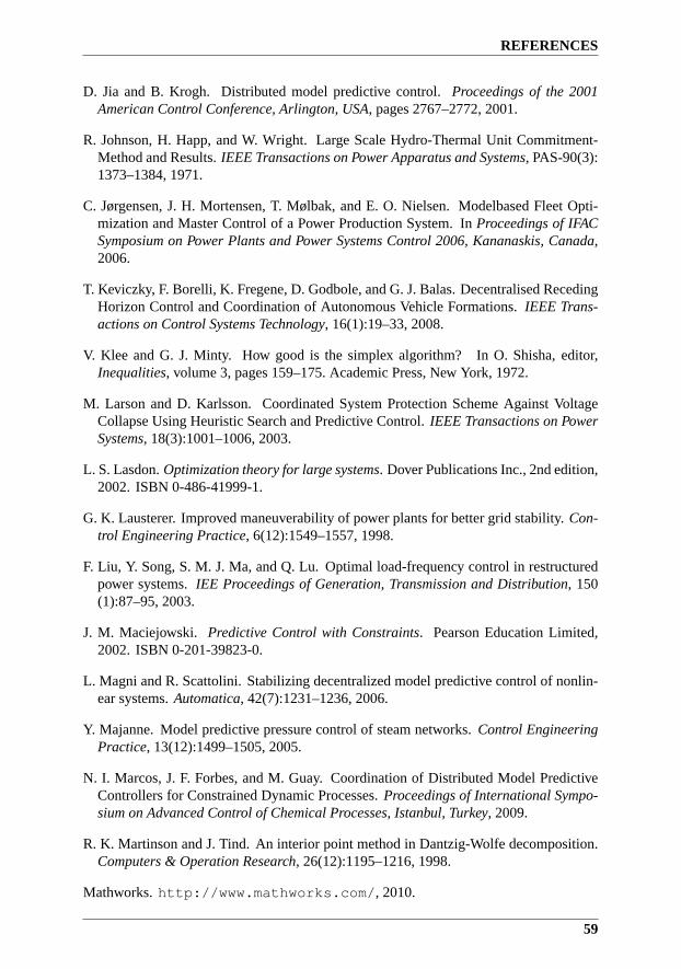
REFERENCES
D. Jia and B. Krogh. Distributed model predictive control.Proceedings of the 2001American Control Conference, Arlington, USA, pages 2767–2772, 2001.
R. Johnson, H. Happ, and W. Wright. Large Scale Hydro-ThermalUnit Commitment-Method and Results.IEEE Transactions on Power Apparatus and Systems, PAS-90(3):1373–1384, 1971.
C. Jørgensen, J. H. Mortensen, T. Mølbak, and E. O. Nielsen. Modelbased Fleet Opti-mization and Master Control of a Power Production System. InProceedings of IFACSymposium on Power Plants and Power Systems Control 2006, Kananaskis, Canada,2006.
T. Keviczky, F. Borelli, K. Fregene, D. Godbole, and G. J. Balas. Decentralised RecedingHorizon Control and Coordination of Autonomous Vehicle Formations. IEEE Trans-actions on Control Systems Technology, 16(1):19–33, 2008.
V. Klee and G. J. Minty. How good is the simplex algorithm? In O. Shisha, editor,Inequalities, volume 3, pages 159–175. Academic Press, New York, 1972.
M. Larson and D. Karlsson. Coordinated System Protection Scheme Against VoltageCollapse Using Heuristic Search and Predictive Control.IEEE Transactions on PowerSystems, 18(3):1001–1006, 2003.
L. S. Lasdon.Optimization theory for large systems. Dover Publications Inc., 2nd edition,2002. ISBN 0-486-41999-1.
G. K. Lausterer. Improved maneuverability of power plants for better grid stability.Con-trol Engineering Practice, 6(12):1549–1557, 1998.
F. Liu, Y. Song, S. M. J. Ma, and Q. Lu. Optimal load-frequencycontrol in restructuredpower systems.IEE Proceedings of Generation, Transmission and Distribution, 150(1):87–95, 2003.
J. M. Maciejowski. Predictive Control with Constraints. Pearson Education Limited,2002. ISBN 0-201-39823-0.
L. Magni and R. Scattolini. Stabilizing decentralized model predictive control of nonlin-ear systems.Automatica, 42(7):1231–1236, 2006.
Y. Majanne. Model predictive pressure control of steam networks. Control EngineeringPractice, 13(12):1499–1505, 2005.
N. I. Marcos, J. F. Forbes, and M. Guay. Coordination of Distributed Model PredictiveControllers for Constrained Dynamic Processes.Proceedings of International Sympo-sium on Advanced Control of Chemical Processes, Istanbul, Turkey, 2009.
R. K. Martinson and J. Tind. An interior point method in Dantzig-Wolfe decomposition.Computers & Operation Research, 26(12):1195–1216, 1998.
Mathworks.http://www.mathworks.com/, 2010.
59
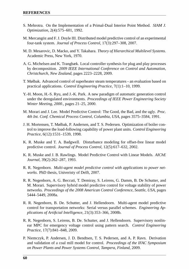
REFERENCES
S. Mehrotra. On the Implementation of a Primal-Dual Interior Point Method. SIAM J.Optimization, 2(4):575–601, 1992.
M. Mercangoz and F. J. Doyle III. Distributed model predictive controlof an experimentalfour-tank system.Journal of Process Control, 17(3):297–308, 2007.
M. D. Mesarovic, D. Macko, and Y. Takahara.Theory of Hierarchical Multilevel Systems.Academic Press, New York, 1970.
A. G. Michelsen and K. Trangbæk. Local controller synthesisfor plug and play processesby decomposition.2009 IEEE International Conference on Control and Automation,Christchurch, New Zealand, pages 2223–2228, 2009.
T. Mølbak. Advanced control of superheater steam temperatures - an evaluation based onpractical applications.Control Engineering Practice, 7(1):1–10, 1999.
Y.-H. Moon, H.-S. Ryu, and J.-K. Park. A new paradigm of automatic generation controlunder the deregulated environments.Proceedings of IEEE Power Engineering SocietyWinter Meeting, 2000., pages 21–25, 2000.
M. Morari and J. Lee. Model Predictive Control: The Good, theBad, and the ugly.Proc.4th Int. Conf. Chemical Process Control, Columbia, USA, pages 3575–3584, 1991.
J. H. Mortensen, T. Mølbak, P. Andersen, and T. S. Pedersen. Optimization of boiler con-trol to improve the load-following capability of power plant units.Control EngineeringPractice, 6(12):1531–1539, 1998.
K. R. Muske and T. A. Badgwell. Disturbance modeling for offset-free linear modelpredictive control.Journal of Process Control, 12(5):617–632, 2002.
K. R. Muske and J. B. Rawlings. Model Predictive Control withLinear Models.AIChEJournal, 39(2):262–287, 1993.
R. R. Negenborn.Multi-agent model predictive control with applications topower net-works. PhD thesis, Univeristy of Delft, 2007.
R. R. Negenborn, A. G. Beccuti, T. Demiray, S. Leirens, G. Damm, B. De Schutter, andM. Morari. Supervisory hybrid model predictive control forvoltage stability of powernetworks.Proceedings of the 2008 American Control Conference, Seattle, USA, pages5444–5449, 2008a.
R. R. Negenborn, B. De. Schutter, and J. Hellendoorn. Multi-agent model predictivecontrol for transportation networks: Serial versus parallel schemes.Engineering Ap-plications of Artificial Intelligence, 21(3):353–366, 2008b.
R. R. Negenborn, S. Leirens, B. De. Schutter, and J. Hellendoorn. Supervisory nonlin-ear MPC for emergency voltage control using pattern search.Control EngineeringPractice, 17(7):841–848, 2009.
P. Niemczyk, P. Andersen, J. D. Bendtsen, T. S. Pedersen, andA. P. Ravn. Derivationand validation of a coal mill model for control.Proceedings of the IFAC Symposiumon Power Plants and Power Systems Control, Tampera, Finland, 2009.
60

REFERENCES
J. Nocedal and S. J. Wright.Numerical Optimization. Springer, New York, 2nd edition,2006. ISBN 0-387-98793-2.
Nord Pool.http://www.nordpool.com, 2010.
B. J. Odelson, M. R. Rajamani, and J. B. Rawlings. A new autocovariance least-squaresmethod for estimating noise covariance.Automatica, 42(2):303–308, 2006.
N. P. Padhy. Unit Commitment - A Bibliographical Survey.IEEE Transactions on PowerSystems, 19(2):1196–1205, 2004.
G. Pannocchia and J. B. Rawlings. Disturbance Models for Offset-Free Model-PredictiveControl. AIChE Journal, 49(2):426–437, 2003.
G. Pannocchia, N. Laachi, and J. B. Rawlings. A Fast, Easily Tuned, SISO, Model Pre-dictive Controller. InDYCOPS 7, 5-7 July 2004, Boston, USA, 2004.
G. Pannocchia, N. Laachi, and J. B. Rawlings. A Candidate to Replcace PID Control:SISO-Constrained LQ Control.AIChE Journal, 51(4):1178–1189, 2005.
S. J. Qin and T. A. Badgwell. An Overview Of Industrial Model Predictive ControlTechnology. InProceedings of AIChE Symposium Series, pages 232–256, 1997.
S. J. Qin and T. A. Badgwell. A survey of industrial model predictive control technology.Control Engineering Practice, 11(7):733–764, 2003.
D. M. Raimondo, L. Magni, and R. Scattolini. Decentralized MPC of nonlinear systems:An input-to-state stability approach.International Journal of Robust and NonlinearControl, 17(17):1651–1667, 2007.
H. Raj. A Distributed Control Algorithm for AGC in Hydrothermal Power Plants.Pro-ceedings of 2006 IFAC Symposium on Power Plants and Power Systems Control,Kananaskis, Canada, 2006.
M. R. Rajamani and J. B. Rawlings. Estimation of the disturbance structure from datausing semidefinite programming and optimal weighting.Automatica, 45(1):142–148,2009.
A. Rantzer. Dynamic Dual Decomposition for Distributed Control. Proceedings of the2009 conference on American Control Conference, St. Louis,USA, pages 884–888,2009.
C. V. Rao and J. B. Rawlings. Linear Programming and Model Predictive Control.Jour-nal of Process Control, 10(2–3):283–289, 2000.
C. V. Rao, S. J. Wright, and J. B. Rawlings. Application of Interior-Point Methods toModel Predictive Control.Journal of Optimization Theory and Applications, 99(3):723–757, 1998.
J. B. Rawlings and R. Amrit. Optimizing Process Economic Performance Using ModelPredictive Control. In L. Magni, D. M. Raimondo, and F. Allgower, editors,NonlinearModel Predictive Control, pages 119–138. Springer, 2009. ISBN 3-764-36297-9.
61
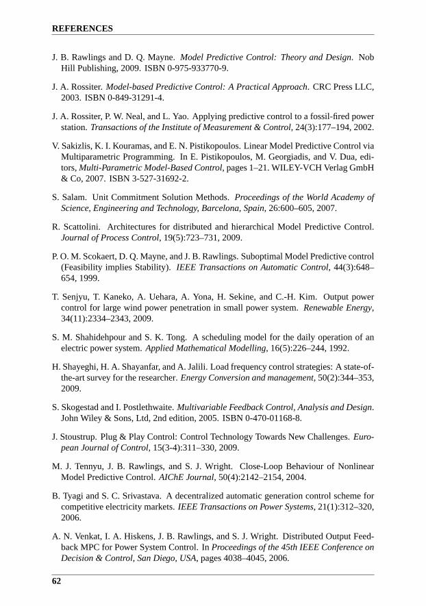
REFERENCES
J. B. Rawlings and D. Q. Mayne.Model Predictive Control: Theory and Design. NobHill Publishing, 2009. ISBN 0-975-933770-9.
J. A. Rossiter.Model-based Predictive Control: A Practical Approach. CRC Press LLC,2003. ISBN 0-849-31291-4.
J. A. Rossiter, P. W. Neal, and L. Yao. Applying predictive control to a fossil-fired powerstation.Transactions of the Institute of Measurement & Control, 24(3):177–194, 2002.
V. Sakizlis, K. I. Kouramas, and E. N. Pistikopoulos. LinearModel Predictive Control viaMultiparametric Programming. In E. Pistikopoulos, M. Georgiadis, and V. Dua, edi-tors,Multi-Parametric Model-Based Control, pages 1–21. WILEY-VCH Verlag GmbH& Co, 2007. ISBN 3-527-31692-2.
S. Salam. Unit Commitment Solution Methods.Proceedings of the World Academy ofScience, Engineering and Technology, Barcelona, Spain, 26:600–605, 2007.
R. Scattolini. Architectures for distributed and hierarchical Model Predictive Control.Journal of Process Control, 19(5):723–731, 2009.
P. O. M. Scokaert, D. Q. Mayne, and J. B. Rawlings. SuboptimalModel Predictive control(Feasibility implies Stability).IEEE Transactions on Automatic Control, 44(3):648–654, 1999.
T. Senjyu, T. Kaneko, A. Uehara, A. Yona, H. Sekine, and C.-H.Kim. Output powercontrol for large wind power penetration in small power system. Renewable Energy,34(11):2334–2343, 2009.
S. M. Shahidehpour and S. K. Tong. A scheduling model for the daily operation of anelectric power system.Applied Mathematical Modelling, 16(5):226–244, 1992.
H. Shayeghi, H. A. Shayanfar, and A. Jalili. Load frequency control strategies: A state-of-the-art survey for the researcher.Energy Conversion and management, 50(2):344–353,2009.
S. Skogestad and I. Postlethwaite.Multivariable Feedback Control, Analysis and Design.John Wiley & Sons, Ltd, 2nd edition, 2005. ISBN 0-470-01168-8.
J. Stoustrup. Plug & Play Control: Control Technology Towards New Challenges.Euro-pean Journal of Control, 15(3-4):311–330, 2009.
M. J. Tennyu, J. B. Rawlings, and S. J. Wright. Close-Loop Behaviour of NonlinearModel Predictive Control.AIChE Journal, 50(4):2142–2154, 2004.
B. Tyagi and S. C. Srivastava. A decentralized automatic generation control scheme forcompetitive electricity markets.IEEE Transactions on Power Systems, 21(1):312–320,2006.
A. N. Venkat, I. A. Hiskens, J. B. Rawlings, and S. J. Wright. Distributed Output Feed-back MPC for Power System Control. InProceedings of the 45th IEEE Conference onDecision & Control, San Diego, USA, pages 4038–4045, 2006.
62

REFERENCES
A. N. Venkat, I. A. Hiskens, J. B. Rawlings, and S. J. Wright. Distributed MPC strategieswith application to power system automatic generation control. IEEE Transaction onControl Systems Technology, 16(6):1192–1206, 2008.
A. Viana, J. P. de Sousa, and M. Matos. Simulated annealing for the unit commitmentproblem.Proceedings of 2001 IEEE Porto Power Tech Proceedings, pages 4–8, 2001.
H. Weber and M. Krueger. Dynamic investigation of network restoration by the pumped-storage plant Markersbach in Germany.Proceedings of the 17th IFAC World Congress,Seoul, Korea, 2008.
H. Weber, T. Hamacher, and T. Haase. Influence on the power station park and the grid.Proceedings of 2006 IFAC Symposium on Power Plants and PowerSystems Control,Kananaskis, Canada, 2006.
E. Welfonder. Least-cost dynamic interaction of power plants and power systems.ControlEngineering Practice, 5(9):1203–1216, 1997.
A. J. Wood and B. F. Wollenberg.Power Generation, Operation and control. John Wiley& sons, inc., 2nd edition, 1996. ISBN 0-471-58699-4.
S. J. Wright. Primal-Dual Interior-Point Methods. SIAM, Philadelphia, 1997. ISBN0-898-71382-4.
Y. Zhang. Solving Large-Scale Linear Programs by Interior-Point Methods under theMatlab Environment.Optimization Methods and Software, 10(1):1–31, 1998.
K. Zhou, J. C. Doyle, and K. Glover.Robust and Optimal Control. Prentice Hall, 1996.ISBN 0-134-56567-3.
63


Contributions
Paper A: Structural Stability Analysis of a Rate Limited Aut omatic Genera-tion Control System
Paper B: Introducing Model Predictive Control for Improving Power PlantPortfolio Performance
Paper C: Simple Models for Model-based Portfolio Load Balancing ControllerSynthesis
Paper D: A Primal-Dual Interior-Point Linear Programming A lgorithm forMPC
Paper E: A Dantzig-Wolfe MPC Algorithm for Power Plant Portfo lio Control
Paper F: Hierarchical model-based predictive control of power plant portfolio


Paper A
Structural Stability Analysis of a Rate Limited AutomaticGeneration Control System
Kristian Edlund, Jan Dimon Bendtsen & Palle Andersen
This paper was published in:Proceedings of the 2009 European Control Conference.

Copyright c©The European Union Control AssociationThe layout has been revised

1 Introduction
Abstract
This paper deals with the the stability analysis of a controller structure used forautomatic generation control (AGC). The AGC structure is derived fromthe litter-ature and augmented to handle generation rate constraints. The derivedstructure isthen compared to the structure of the AGC used within DONG Energy, which re-moves deviations between reference and production. The analysis is conducted ona linear approximation of the closed loop system, with focus on the structureof thecontroller. We show that with the chosen structure, the closed loop system will beinternally unstable independently of the controller parameters. The analysis showsthat the different units in the portfolio might drift in opposite directions, a behavioralso observed in the real system. The drifting ruins the economical optimisation. Theinstability issue can, however, be alleviated by introducing so-called parallel run.
1 Introduction
Controllers in general, and in particular controllers usedfor automatic generation control(AGC), are often implemented with the primary motivation toachieve economic benefitfrom good operation of the plants, which can then be translated into a number of perfor-mance criteria, of which the most fundamental is stabilisation of the system.
The problem of designing AGCs to cooperate among multiple regions has been thesubject of much research lately, both regarding optimalityand stability. However, it ismost often assumed that the generators within the area function as one generator. For ex-ample [Bakken and Grande, 1998] describes how to introduce an AGC in Norway, but thefocus is on the main controller rather than the distributionof the error among the partici-pating generators. Centralised AGC design under constraints is treated in [Hassan et al.,2008] both for single-area and multi-area production, but the area is treated as one gener-ator. In [Venkat et al., 2006; Moon et al., 2000; Tyagi and Srivastava, 2006] decentralisedmodel-based methods for multi-area AGC are developed, but without discussing how todistribute the output from the controller known as the area control error (ACE) amongthe multiple generators in the control area. Focusing on stability, [Azzam and Mohamed,2002] developed a design method for generating a stabilising controller.
[Liu et al., 2003; Chen et al., 2007; Wood and Wollenberg, 1996] describe how todistribute the ACE among the participating generators in the area. [Liu et al., 2003; Chenet al., 2007] deal with control of multiple generators within an area using optimisation-based schemes. However, both treat the problem as a static rather than a dynamic prob-lem. [Wood and Wollenberg, 1996] presents an AGC for distributing the ACE to multiplegenerators based on a PI-controller structure. This structure for distributing the ACE isvery common, and the principle is also used in the internal AGC within DONG Energy,who operates in Denmark. The work in [Wood and Wollenberg, 1996] will be used as abase for the structure in this paper and will be further discussed in section 3. However, aswill be shown, in case of load disturbances, it is required tomodify the scheme in orderto maintain stability.
The outline of the rest of the paper is as follows: Section 2 describes the set of as-sumptions and requirements for the controller and the system. This is followed by a dis-cussion of the augmentation of the structure needed to fulfill the requirements in section3. Section 4 presents an analysis of the stability of the augmented structure. A numerical
69
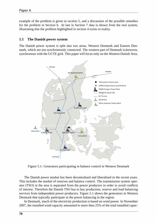
Paper A
example of the problem is given in section 5, and a discussionof the possible remediesfor the problem in Section 6. At last in Section 7 data is shownfrom the real system,illustrating that the problem highlighted in section 4 exists in reality.
1.1 The Danish power system
The Danish power system is split into two areas, Western Denmark and Eastern Den-mark, which are not synchronously connected. The western part of Denmark is,however,synchronous with the UCTE grid. This paper will focus only onthe Western Danish Area.
Studstrupværket
Herningværket
DONG Energy's Power Plant
DONG Energy Central Control Room
TSO Central Control room
Horns Rev 1
400 KV AC power line
DC Tie Line
Wind farm
Nordjyllandsværket
Other producers Power plant
Norway
Sweden
Esbjergværket Skærbækværket
Enstedværket
Horns Rev 1
Fynsværket
Germany
Figure 5.1: Generators participating in balance control inWestern Denmark
The Danish power market has been decentralised and liberalised in the recent years.This includes the market of reserves and balance control. The transmission system oper-ator (TSO) in the area is separated from the power producers in order to avoid conflictsof interest. Therefore the Danish TSO has to buy production,reserve and load balancingservices from independent power producers. Figure 5.1 shows the generators in WesternDenmark that typically participate in the power balancing in the region.
In Denmark, much of the electricity production is based on wind power. In November2007, the installed wind capacity amounted to more than 25% of the total installed capac-
70

1 Introduction
ity. The Western Danish area functions as one area with multiple generators, which meansthat a primary concern when designing an AGC is how to distribute the ACE between thegenerators. Therefore an AGC is applied to regulate the fastfluctuations caused by thewind power [UCTE, 2007].
The commissioned AGC works in a deregulated market and is split up between theTSO and multiple independent power generating companies. The Danish TSO, generatesan area control error (ACE) and distributes it among the companies participating in thebalance control of the Danish power system. The individual producer is then responsiblefor distributing its share of the ACE among the generators operated by the company. Eachproducer also has the responsibility for maintaining the balance between the actual andordered production within the portfolio of generators.
The fast fluctuations in the power system must be suppressed by thermal generators,which are dominant in the power system. Therefore the thermal generators will oftenreach their rate limit at typically 4% load/minute, and therefore the AGC must be ableto handle the fact that the generators reach the generation rate constraints a significantpercentage of the time. It is noted in [Wood and Wollenberg, 1996] that an AGC shouldbe able to handle this, but no specific method is given. In practice, it is often done with aPI-controller structure augmented with a set of so-calledparticipation factorsto split theload among the participating plants.
Due to the fast fluctuations in the Danish power system, the set of participation fac-tors is changed very often. Existing literature does not seem to have investigated whatinfluence a rate limit constraint has on the stability of the distribution of the ACE withinthe power system.
TSO
Economic Dispatch
(Production Planning)
+Portfolio
MW
MW
MWDeviation
Production plan
Measured production
Load balancing
controller
-
+
Reference
feedforward
Disturbances
AGC signal
Filter
Expected
Response
Figure 5.2: System level control within DONG Energy.
The system level control within DONG Energy is depicted in Figure 5.2 and furtherdescribed in [Jørgensen et al., 2006]. This paper concentrates on the load balancing con-troller. It gets an input from the production sold on the Power Exchange and the shareof the ACE coming from the TSO. Adding these gives the total portfolio reference whichhas to be followed.
This paper deals with analysis of the stability of an AGC whencompensation forgeneration rate constraints are added to the controller. The analysis is conducted basedon a linearised model of the power system.
71
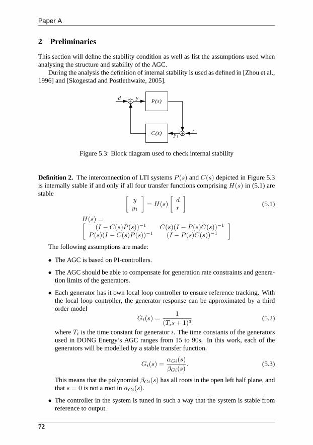
Paper A
2 Preliminaries
This section will define the stability condition as well as list the assumptions used whenanalysing the structure and stability of the AGC.
During the analysis the definition of internal stability is used as defined in [Zhou et al.,1996] and [Skogestad and Postlethwaite, 2005].
P(s)
C(s)
+
+
d
y1
r
y
Figure 5.3: Block diagram used to check internal stability
Definition 2. The interconnection of LTI systemsP (s) andC(s) depicted in Figure 5.3is internally stable if and only if all four transfer functions comprisingH(s) in (5.1) arestable
[
yy1
]
= H(s)
[
dr
]
(5.1)
H(s) =[
(I − C(s)P (s))−1 C(s)(I − P (s)C(s))−1
P (s)(I − C(s)P (s))−1 (I − P (s)C(s))−1
]
The following assumptions are made:
• The AGC is based on PI-controllers.
• The AGC should be able to compensate for generation rate constraints and genera-tion limits of the generators.
• Each generator has it own local loop controller to ensure reference tracking. Withthe local loop controller, the generator response can be approximated by a thirdorder model
Gi(s) =1
(Tis+ 1)3(5.2)
whereTi is the time constant for generatori. The time constants of the generatorsused in DONG Energy’s AGC ranges from15 to 90s. In this work, each of thegenerators will be modelled by a stable transfer function.
Gi(s) =αGi(s)
βGi(s). (5.3)
This means that the polynomialβGi(s) has all roots in the open left half plane, andthats = 0 is not a root inαGi(s).
• The controller in the system is tuned in such a way that the system is stable fromreference to output.
72
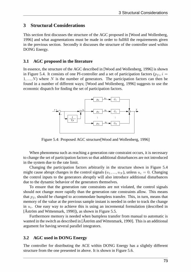
3 Structural Considerations
3 Structural Considerations
This section first discusses the structure of the AGC proposed in [Wood and Wollenberg,1996] and what augmentations must be made in order to fullfillthe requirements givenin the previous section. Secondly it discusses the structure of the controller used withinDONG Energy.
3.1 AGC proposed in the literature
In essence, the structure of the AGC described in [Wood and Wollenberg, 1996] is shownin Figure 5.4. It consists of one PI-controller and a set of participation factors (pfi, i =1, ..., N ) whereN is the number of generators. The participation factors can then befound in a number of different ways; [Wood and Wollenberg, 1996] suggests to use theeconomic dispatch for finding the set of participation factors.
1Tis
pf1
pf2
pfN
-
++
G1
G2
GN
+
u1
uc u2
u3
... ...
yr
Figure 5.4: Proposed AGC structure[Wood and Wollenberg, 1996]
When phenomena such as reaching a generation rate constraintoccurs, it is necessaryto change the set of participation factors so that additional disturbances are not introducedin the system due to the rate limit.
Changing the participation factors arbitrarily in the structure shown in Figure 5.4might cause abrupt changes in the control signals (u1, ..., uN ), unlessuc = 0. Changingthe control inputs to the generators abruptly will also introduce additional disturbancesdue to the dynamic behavior of the generators themselves.
To ensure that the generation rate constraints are not violated, the control signalsshould not change more rapidly than the generation rate constraints allow. This meansthatpfi should be changed to accommodate bumpless transfer. This, in turn, means thatmemory of the value at the previous sample instant is needed in order to track the changein ui. One easy way to achieve this is using an incremental formulation (described in[Astrom and Wittenmark, 1990]), as shown in Figure 5.5.
Furthermore memory is needed when bumpless transfer from manual to automatic iswanted in the switch as described in [Astrom and Wittenmark, 1990]. This is an additionalargument for having several parallel integrators.
3.2 AGC used in DONG Energy
The controller for distributing the ACE within DONG Energy has a slightly differentstructure from the one presented in above. It is shown in Figure 5.6.
73

Paper A
1Tis
x
-
++
G1
G2
GN
+
u1
uc
s s-1
pf1
xs s-1
pf2
xs s-1
pfN
u2
uN
r y
...
......
Figure 5.5: Alternative structure of the AGC with incremental implementation.
-
+
G1
yG2
GN
PI1
PI2
PIN
+r
...
...
Figure 5.6: Structure of the AGC within DONG Energy
The reference is distributed to a set of PI-controllers withgain scheduling. The gainsare recomputed every0.5 seconds according to factors such as generation rate constraints.
In order to compensate for generation rate constraints, theAGC structure used withinDONG Energy has to be augmented in a similar fashion. The result is shown in Figure5.7. The structure has a behaviour similar to the structure shown previously.
-
++
G1
G2
GN
s x
x1Ti
kp1
kp1
s-1
s x
x
s-1
1Ti
s x
x1Ti
s-1
kp2
kp2
kpN
kpN
+
+
+
y
......
.....
.
r
Figure 5.7: Current structure of the AGC
74

4 Stability of an AGC
4 Stability of an AGC
In the previous section it was argued that, in order to compensate for the generation rateconstraints, it is necessary to have memory about each generator, which can for instancebe added in terms of integrators. In this section, the stability of a structure with parallelintegrators will be analysed. The participation factors are calculated at each sample, andis based on the constraints and limits. Therefore the participation factors often changerapidly, in particular whenever∆uc changes sign. This behaviour will be treated as adisturbance entering the system close topfi.
4.1 AGC with compensation for changes inpfi
For the analysis the system is grouped into subsystems as shown in Figure 5.8.
1Tis
x
-
++
G1
G2
GN
+
y1s s-1
pf1
xs s-1
pf2
xs s-1
pfN
r y
+
dc1 g1
g2c0
... ... ...
Figure 5.8: Subsystems used for analysis of AGC with compensation for changes inpfi
where the transfer function of each subsystem can be described as
g1(s) =αG1
sβG1, g2(s) =
αG2
βG2, c1(s) = s, c0(s) = 1 +
1
Tis(5.4)
g2(s) contains the generatorsGi wherei = 2, ..., N . αG1 is assumed not to have aroot ins = 0. We now have the following result.
Theorem 2. The structure shown in Figure 5.8 is internally unstable forany choice ofcontroller parameters under the assumptions listed in section 2.
Proof. By showing that at least one of the transfer functions in (5.1) cannot be stabilisedfor any choice of controller parameter, it is proven that thesystem is internally unstable.
The transfer function matrix is shown in (5.5) on the next page.
All transfer functions except the bottom left has the same denominator. Sincey(s)r(s) is
stable by assumption, all three transfer functions are stable. However,y1(s)d(s) has a zero
in s = 0, sinces = 0 is not a root in the nominator polynomial it is not cancelled.Thisclosed right half plane pole in the transfer function cannotbe eliminated by any choice ofcontroller parameters, and the structure is therefore internally unstable.
75
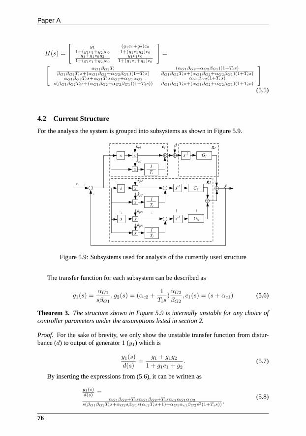
Paper A
H(s) =
[
g1
1+(g1c1+g2)c0
(g1c1+g2)c0
1+(g1c1g2)c0g1+g1c0g2
1+(g1c1+g2)c0
g1c1c0
1+(g1c1+g2)c0
]
=
[
αG1βG2Ti
βG1βG2Tis+(αG1βG2+αG2βG1)(1+Tis)(αG1βG2+αG2βG1)(1+Tis)
βG1βG2Tis+(αG1βG2+αG2βG1)(1+Tis)αG1βG2Tis+αG1TisαG2+αG1αG2
s(βG1βG2Tis+(αG1βG2+αG2βG1)(1+Tis))αG1βG2(1+Tis)
βG1βG2Tis+(αG1βG2+αG2βG1)(1+Tis)
]
(5.5)
4.2 Current Structure
For the analysis the system is grouped into subsystems as shown in Figure 5.9.
-
++
G1
G2
G�
s x
x1
Ti
kp1
kp1
s-1
s x
x
s-1
1
Ti
s x
x1
Ti
s-1
kp2
kp2
kp�
kp�
+
+
+
y
+
d
++
c1 g1
g2r
...
...
...
...
Figure 5.9: Subsystems used for analysis of the currently used structure
The transfer function for each subsystem can be described as
g1(s) =αG1
sβG1, g2(s) = (αc2 +
1
Tis)αG2
βG2, c1(s) = (s+ αc1) (5.6)
Theorem 3. The structure shown in Figure 5.9 is internally unstable forany choice ofcontroller parameters under the assumptions listed in section 2.
Proof. For the sake of brevity, we only show the unstable transfer function from distur-bance (d) to output of generator 1 (y1) which is
y1(s)
d(s)=
g1 + g1g21 + g1c1 + g2
. (5.7)
By inserting the expressions from (5.6), it can be written as
y1(s)d(s) =
αG1βG2+TisαG1βG2+Tisαc2αG1αG2
s(βG1βG2Tis+αG2sβG1s(αc2Tis+1)+αG1αc1βG2s2(1+Tis)).
(5.8)
76

5 Numerical Example
This transfer function has a root ins = 0 in the denominator, and sinces = 0 is not a rootin the nominator polynomial it is not cancelled. The root ins = 0 cannot be cancelled byany choice of controller parameters, and the structure is therefore internally unstable.
5 Numerical Example
In this section, a numerical example is shown for the structure shown in Theorem 2.It corresponds to the structure proposed in [Wood and Wollenberg, 1996], except thatit is modified to accommodate generation rate constraints. The system consists of twogenerators, where the dynamics can be modelled as two third order systems as shown inFigure 5.10.
1(50s+1)3
1200s
x
-
+++
y1s 1/s
xs
r y
1(40s+1)3
1/sy2
f1(x)
f2(x)d
Figure 5.10: Example AGC with compensation for changes inpfi
The participation factors are calculated using the simple functions
f1(x) =
{
0.4 x ≤ 00.6 x > 0
and f2(x) =
{
0.6 x ≤ 00.4 x > 0
The changing participa-
tion factors are used in order to exploit the full rate of change possible when there areasymmetric rate limits.d is zero-mean white noise added to the output with varianceσ2 = 0.001.
0 500 1000 1500 2000−4
−2
0
2
4
6
8
10
12
14
Time [sec]
Out
put [
MW
]
Total OutputReferenceGenerator 1Generator 2
Figure 5.11: Simulation of AGC with compensation for changes inpfi
77

Paper A
-+ +
G1s x
x1Ti
pf1
pf1s-1
pfN
+
y
Kpr/N+ -
+
G2s x
x1Ti
pf2
pf2s-1+
+
GNs x
x1Ti
pfNs-1+
+
+ -
+ -
...
... ... ...
Figure 5.12: Controller with parallel run
Figure 5.11 show the result of a simulation of the system shown in Figure 5.10 usinga sample time of 1 second. The results shows that the controller is capable of followingthe reference, but the generators drift in opposite directions, as predicted by the internalinstability results shown in the previous section.
6 Stabilisation of the structure
In this section, we present two different ways to remedy the internal instability of thesystem as well as a discussion of pros and cons of the two solutions. Both solutions havebeen applied to the controller within DONG Energy.
6.1 Parallel run
Parallel run is commonly used within the power plant industry when two similar subsys-tems have to work in parallel to complete a task. When using PI-controllers in parallel,the subsystems will in general not contribute equally when the equilibrium is reached. Inorder to obtain this behaviour, parallel run is introduced.In the AGC system, the genera-tors are treated as parallel subsystems, which contribute to achieve an overall goal. Figure5.12 shows how the parallel run is introduced.
The parallel run drives the integrators towards the same value, and thereby ensures thatthe behaviour seen in the example above where to generators drift in opposite directionsis avoided. Choosing the parallel run, parameterKpr is a trade off between forcing theintegrators towards each other, and obtaining good reference tracking. If the gainKpr
is too large, the parallel run may in some situations dominate the controller behaviour,ruining the reference tracking capability.
Gain scheduling of the parallel run as a function of the change in ACE might bea solution to overcome balancing between not interfering onthe control power and noeffect from the parallel run.
78
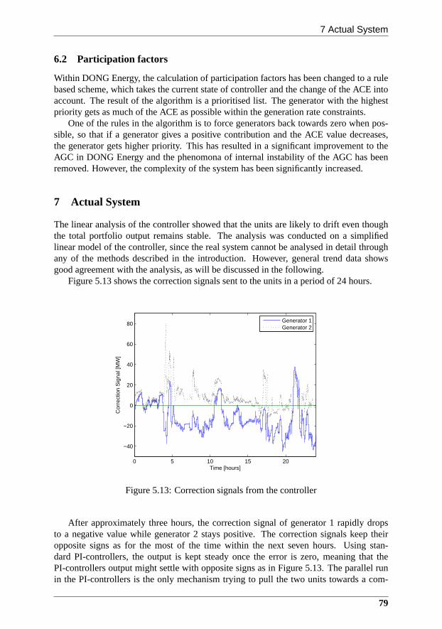
7 Actual System
6.2 Participation factors
Within DONG Energy, the calculation of participation factors has been changed to a rulebased scheme, which takes the current state of controller and the change of the ACE intoaccount. The result of the algorithm is a prioritised list. The generator with the highestpriority gets as much of the ACE as possible within the generation rate constraints.
One of the rules in the algorithm is to force generators back towards zero when pos-sible, so that if a generator gives a positive contribution and the ACE value decreases,the generator gets higher priority. This has resulted in a significant improvement to theAGC in DONG Energy and the phenomona of internal instabilityof the AGC has beenremoved. However, the complexity of the system has been significantly increased.
7 Actual System
The linear analysis of the controller showed that the units are likely to drift even thoughthe total portfolio output remains stable. The analysis wasconducted on a simplifiedlinear model of the controller, since the real system cannotbe analysed in detail throughany of the methods described in the introduction. However, general trend data showsgood agreement with the analysis, as will be discussed in thefollowing.
Figure 5.13 shows the correction signals sent to the units ina period of 24 hours.
0 5 10 15 20
−40
−20
0
20
40
60
80
Time [hours]
Cor
rect
ion
Sig
nal [
MW
]
Generator 1Generator 2
Figure 5.13: Correction signals from the controller
After approximately three hours, the correction signal of generator 1 rapidly dropsto a negative value while generator 2 stays positive. The correction signals keep theiropposite signs as for the most of the time within the next seven hours. Using stan-dard PI-controllers, the output is kept steady once the error is zero, meaning that thePI-controllers output might settle with opposite signs as in Figure 5.13. The parallel runin the PI-controllers is the only mechanism trying to pull the two units towards a com-
79
Paper A
mon correction, so that they contribute equally. However, the parallel run is too weakcompared to the noise and the change in reference to succeed in this case.
The explanation for the units drifting from the production plan is found in the distri-bution of the controller gain and the rate limiter. The controller has two different gains,one for positive error, and one for negative error. The result is that one unit ends up witha large part of the contribution in one direction and the other unit ends up with a largepart of the contribution in the other direction. When the error is positive, both units re-ceive commands to follow a step up, but one unit gets a larger step than the other. Whenthe error changes sign, both units correspondingly receiveorders to follow a step down,but the other unit then gets a much larger step than the first. When the error is closeto zero, it often changes sign, which over time results in oneunit accumulating a largepositive correction and one unit accumulating a large negative correction. Overall, thisbehaviour is quite similar to the behaviour observed by introducing disturbances in thelinaer approximation treated in section 4.
The units are saved from drifting too far apart for three mainreasons. The systems arelimited, so that one unit cannot deviate more than a certain amount from the productionplan without manual intervention from the operator. These limits ensure that the units arenot drifting too much. The parallel run is a gain multiplied with an error, so the largerthe span between two units, the stronger the parallel run is.And last but not least, thereare steady periods where the reference from the TSO is close to steady state, giving theparallel run a chance of pulling the units together again.
8 Discussion
A set of assumptions and requirements commonly found in literature for an AGC hasbeen summarised and analysed. In order to fulfill this set of requirements, it is argued thatthe system must be structured in a certain way. However, it was also found that such asystem is internally unstable. The instability shows in fact that generators participating thebalance control has a tendency to drift in opposite directions. Data from a real productionenvironment supports this conclusion. The drifting of the generators ruin the economicaloptimisation of the system.
Two different ways to remedy the problem have been proposed -parallel run andchanges in the calculation of participation factors. It is found that in practice, the parallelrun is insufficient to force the drifting generators towardsthe same value.
Another solution is to change the calculation of the participation factors. A rule-basedsystem has been set up within DONG Energy, and rules have beenadded to ensure thatthe generators are forced back to the production plan when possible. The system workswell, and the drifting is no longer seen. However, the systembehavior is now far moredifficult to analyse in case of problems.
The favoured remedy is the last proposed, but due to the complexity of this solution,a better approach might be to reduce the requirement that theAGC should be based onPI-controllers. This is an indication that it may prove advantageous to introduce model-based MIMO control in the future.
80
8 Discussion
References
K. J. Astrom and B. Wittenmark.Computer-controlled Systems. Prentice Hall, 3rd edi-tion, 1990. ISBN 0-133-14899-8.
M. Azzam and Y. S. Mohamed. Robust controller design for automatic generation controlbased on Q-parameterization.Energy Conversion and Management, 1(43):1663–1673,2002.
B. H. Bakken and O. S. Grande. Automatic Generation Control in a Deregulated PowerSystem.IEEE Transactions on Power Systems, 13(4):1401–1406, 1998.
L. Chen, J. Zhong, and D. Gan. Optimal Automatic Generation Control (AGC) Dis-patching and Its Control Performance Analysis for the Distribution Systems with DGs.Power Engineering Society General Meeting, 2007, Tampa, USA, pages 1–6, 2007.
M. F. Hassan, A. A. Abouelsoud, and H. M. Soliman. Constrained Load-frequency Con-trol. Electric Power Components and Systems, 36(3):266–279, 2008.
C. Jørgensen, J. H. Mortensen, T. Mølbak, and E. O. Nielsen. Modelbased Fleet Opti-mization and Master Control of a Power Production System. InProceedings of IFACSymposium on Power Plants and Power Systems Control 2006, Kananaskis, Canada,2006.
F. Liu, Y. Song, S. M. J. Ma, and Q. Lu. Optimal load-frequencycontrol in restructuredpower systems.IEE Proceedings of Generation, Transmission and Distribution, 150(1):87–95, 2003.
Y.-H. Moon, H.-S. Ryu, and J.-K. Park. A new paradigm of automatic generation controlunder the deregulated environments.Proceedings of IEEE Power Engineering SocietyWinter Meeting, 2000., pages 21–25, 2000.
S. Skogestad and I. Postlethwaite.Multivariable Feedback Control, Analysis and Design.John Wiley & Sons, Ltd, 2nd edition, 2005. ISBN 0-470-01168-8.
B. Tyagi and S. C. Srivastava. A decentralized automatic generation control scheme forcompetitive electricity markets.IEEE Transactions on Power Systems, 21(1):312–320,2006.
UCTE. European Wind Integration Study (EWIS) Towards a successful integration ofwind power into european electricity grids. Technical report, UCTE, 2007.
A. N. Venkat, I. A. Hiskens, J. B. Rawlings, and S. J. Wright. Distributed Output Feed-back MPC for Power System Control. InProceedings of the 45th IEEE Conference onDecision & Control, San Diego, USA, pages 4038–4045, 2006.
A. J. Wood and B. F. Wollenberg.Power Generation, Operation and control. John Wiley& sons, inc., 2nd edition, 1996. ISBN 0-471-58699-4.
K. Zhou, J. C. Doyle, and K. Glover.Robust and Optimal Control. Prentice Hall, 1996.ISBN 0-134-56567-3.
81

Paper B
Introducing Model Predictive Control for Improving Power Pl antPortfolio Performance
Kristian Edlund, Jan Dimon Bendtsen, Simon Børresen & Tommy Mølbak
This paper was published in:Proceedings of the 17th IFAC World Congress

Copyright c©International Federation of Automatic ControlThe layout has been revised
1 Introduction
Abstract
This paper introduces a model predictive control (MPC) approach to constructionof a controller for balancing power generation against consumption in a power sys-tem. The objective of the controller is to coordinate a portfolio consisting of multiplepower plant units in an effort to perform reference tracking and disturbance rejectionin an economically optimal way. The performance function is chosen as amixtureof the ℓ1-norm and a linear weighting to model the economics of the system. Sim-ulations show a significant improvement of the performance of the MPC comparedto the current implementation consisting of a distributed PI controller structure, bothin terms of minimising the overall cost but also in terms of the ability to minimisedeviation, which is the classical objective.
1 Introduction
This paper focuses on the power system in the western part of Denmark, where DONGEnergy [DONG Energy, 2007]is the largest power producer. Being a major power pro-ducer also means that DONG Energy provides a major part of thebalancing reserves forthe transmission system operator (TSO), who has the overallload balancing responsibil-ity. Load balancing means making the production equal to theconsumption. In 2007approximately 30% of the installed capacity in West Denmarkwas wind turbines - a largeshare compared to other areas of Europe. This makes balance control a difficult issuedue to the stochastic behaviour of the wind-based production. Today, balancing can bedone partly by exporting the electricity to other parts of Europe and partly by adjustingthe load of the other production units. However, with the increasing integration of windpower the current balance control system must be improved inorder to be able to handlethe changing conditions in the future.
The deregulation and decentralisation of the European power system complicate co-ordination of control actions. In [UCTE, 2007] it is predicted that a significant numberof wind turbines will be installed in Europe. This will introduce more stochastic pro-duction, which calls for improved control of the power system to balance production andconsumption in order to avoid large blackouts in the future.
The fluctuation in Denmark introduced by the wind turbines has made it necessary tocommission an AGC (Automatic Generation Control) which is able to activate a reserveof ±140MW to take care of small and quick deviations [UCTE, 2007]. This AGC iscontrolled by the TSO, which sends an activation signal to the balancing participants,who are then responsible for activating the required reserves. The reserves are activatedby changing the load distribution among a portfolio of powerplants.
The controller which distributes the reserve activation within the DONG Energy port-folio is responsible for maintaining the load balance within the portfolio on a seconds-to-minutes horizon, until the economic dispatch can take over and handle the short term(minutes-to-hours) load balancing. The controller is therefore referred to as the load bal-ancing controller, not to be mistaken for the AGC at the TSO.
The portfolio is a very complex system and the optimisation and control are thereforeordered in a hierarchical fashion in order to break down the complexity as described in[Jørgensen et al., 2006]. The economic dispatch as well as the load balancing are handledmainly on the system level as described in [Jørgensen et al.,2006].
85
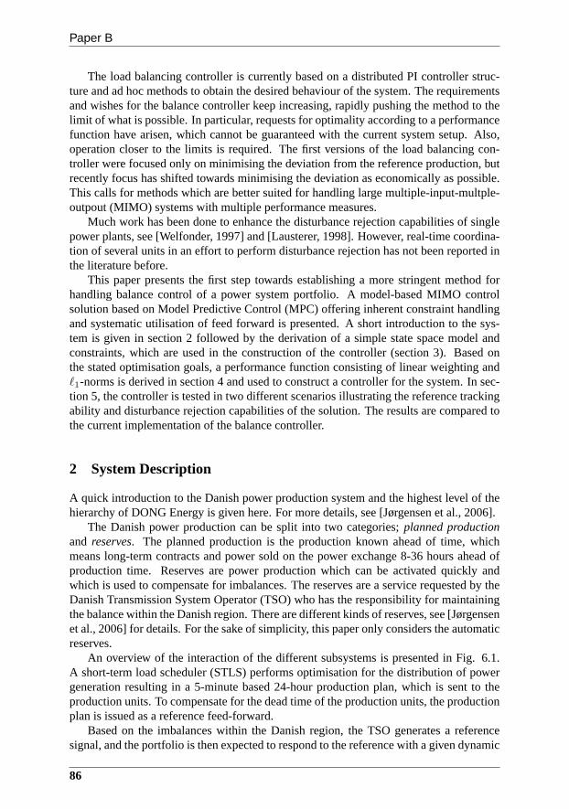
Paper B
The load balancing controller is currently based on a distributed PI controller struc-ture and ad hoc methods to obtain the desired behaviour of thesystem. The requirementsand wishes for the balance controller keep increasing, rapidly pushing the method to thelimit of what is possible. In particular, requests for optimality according to a performancefunction have arisen, which cannot be guaranteed with the current system setup. Also,operation closer to the limits is required. The first versions of the load balancing con-troller were focused only on minimising the deviation from the reference production, butrecently focus has shifted towards minimising the deviation as economically as possible.This calls for methods which are better suited for handling large multiple-input-multple-outpout (MIMO) systems with multiple performance measures.
Much work has been done to enhance the disturbance rejectioncapabilities of singlepower plants, see [Welfonder, 1997] and [Lausterer, 1998].However, real-time coordina-tion of several units in an effort to perform disturbance rejection has not been reported inthe literature before.
This paper presents the first step towards establishing a more stringent method forhandling balance control of a power system portfolio. A model-based MIMO controlsolution based on Model Predictive Control (MPC) offering inherent constraint handlingand systematic utilisation of feed forward is presented. A short introduction to the sys-tem is given in section 2 followed by the derivation of a simple state space model andconstraints, which are used in the construction of the controller (section 3). Based onthe stated optimisation goals, a performance function consisting of linear weighting andℓ1-norms is derived in section 4 and used to construct a controller for the system. In sec-tion 5, the controller is tested in two different scenarios illustrating the reference trackingability and disturbance rejection capabilities of the solution. The results are compared tothe current implementation of the balance controller.
2 System Description
A quick introduction to the Danish power production system and the highest level of thehierarchy of DONG Energy is given here. For more details, see[Jørgensen et al., 2006].
The Danish power production can be split into two categories; planned productionand reserves. The planned production is the production known ahead of time, whichmeans long-term contracts and power sold on the power exchange 8-36 hours ahead ofproduction time. Reserves are power production which can beactivated quickly andwhich is used to compensate for imbalances. The reserves area service requested by theDanish Transmission System Operator (TSO) who has the responsibility for maintainingthe balance within the Danish region. There are different kinds of reserves, see [Jørgensenet al., 2006] for details. For the sake of simplicity, this paper only considers the automaticreserves.
An overview of the interaction of the different subsystems is presented in Fig. 6.1.A short-term load scheduler (STLS) performs optimisation for the distribution of powergeneration resulting in a 5-minute based 24-hour production plan, which is sent to theproduction units. To compensate for the dead time of the production units, the productionplan is issued as a reference feed-forward.
Based on the imbalances within the Danish region, the TSO generates a referencesignal, and the portfolio is then expected to respond to the reference with a given dynamic
86
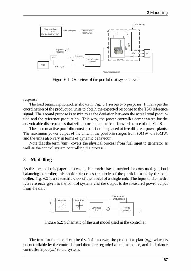
3 Modelling
TSO
Short-term load scheduler
(Production Planning)
+ Portfolio
MW
MW
MW Deviation
Production plan
Measured production
Load balancing controller
-
+
Reference feedforward
Disturbances
AGC signal
Filter
Expected Response
Figure 6.1: Overview of the portfolio at system level
response.The load balancing controller shown in Fig. 6.1 serves two purposes. It manages the
coordination of the production units to obtain the expectedresponse to the TSO referencesignal. The second purpose is to minimise the deviation between the actual total produc-tion and the reference production. This way, the power controller compensates for theunavoidable discrepancies that will occur due to the feed-forward nature of the STLS.
The current active portfolio consists of six units placed atfive different power plants.The maximum power output of the units in the portfolio rangesfrom 80MW to 650MW,and the units also vary in terms of dynamic behaviour.
Note that the term ’unit’ covers the physical process from fuel input to generator aswell as the control system controlling the process.
3 Modelling
As the focus of this paper is to establish a model-based method for constructing a loadbalancing controller, this section describes the model of the portfolio used by the con-troller. Fig. 6.2 is a schematic view of the model of a single unit. The input to the modelis a reference given to the control system, and the output is the measured power outputfrom the unit.
Low pass filter u
c y
Proces dynamics
Min/max Rate limit
+
u p
Unmeasured Disturbance
Figure 6.2: Schematic of the unit model used in the controller
The input to the model can be divided into two; the productionplan (up), which isuncontrollable by the controller and therefore regarded asa disturbance, and the balancecontroller input (uc) to the system.
87
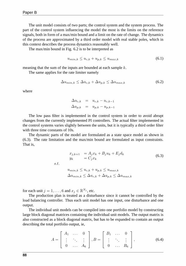
Paper B
The unit model consists of two parts; the control system and the system process. Thepart of the control system influencing the model the most is the limits on the referencesignals, both in form of a max/min bound and a limit on the rateof change. The dynamicsof the process are approximated by a third order model with real stable poles, which inthis context describes the process dynamics reasonably well.
The max/min bound in Fig. 6.2 is to be interpreted as
umin,k ≤ uc,k + up,k ≤ umax,k (6.1)
meaning that the sum of the inputs are bounded at each samplek.The same applies for the rate limiter namely
∆umin,k ≤ ∆uc,k + ∆up,k ≤ ∆umax,k (6.2)
where
∆uc,k = uc,k − uc,k−1
∆up,k = up,k − up,k−1
The low pass filter is implemented in the control system in order to avoid abruptchanges from the currently implemented PI controllers. Theactual filter implemented inthe control systems varies slightly between the units, but it is typically a third order filterwith three time constants of 10s.
The dynamic parts of the model are formulated as a state spacemodel as shown in(6.3). The rate limitation and the max/min bound are formulated as input constraints.That is,
xj,k+1 = Ajxk +Bjuk + Ejdk
yk = Cjxk(6.3)
s.t.
umin,k ≤ uc,k + up,k ≤ umax,k
∆umin,k ≤ ∆uc,k + ∆up,k ≤ ∆umax,k
for each unitj = 1, . . . , 6 andxj ∈ RNj , etc.
The production plan is treated as a disturbance since it cannot be controlled by theload balancing controller. Thus each unit model has one input, one disturbance and oneoutput.
The individual unit models can be compiled into one portfolio model by constructinglarge block diagonal matrices containing the individual unit models. The output matrix isalso constructed as a block diagonal matrix, but has to be expanded to contain an outputdescribing the total portfolio output, ie,
A =
A1 . . . 0...
. .....
0 . . . A6
, B =
B1 . . . 0...
. .....
0 . . . B6
, (6.4)
88
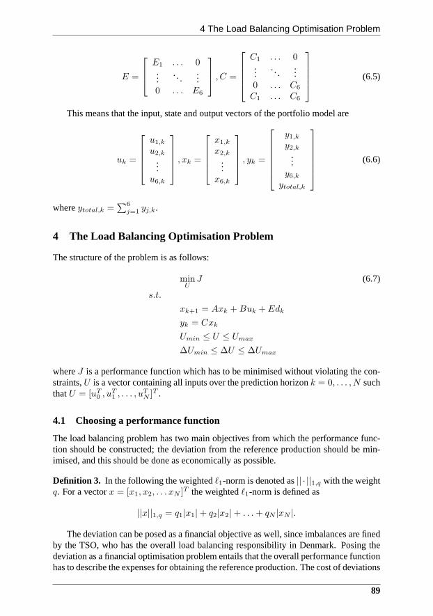
4 The Load Balancing Optimisation Problem
E =
E1 . . . 0...
. . ....
0 . . . E6
, C =
C1 . . . 0...
.. ....
0 . . . C6
C1 . . . C6
(6.5)
This means that the input, state and output vectors of the portfolio model are
uk =
u1,k
u2,k
...u6,k
, xk =
x1,k
x2,k
...x6,k
, yk =
y1,k
y2,k
...y6,k
ytotal,k
(6.6)
whereytotal,k =∑6
j=1 yj,k.
4 The Load Balancing Optimisation Problem
The structure of the problem is as follows:
minU
J (6.7)
s.t.
xk+1 = Axk +Buk +Edk
yk = Cxk
Umin ≤ U ≤ Umax
∆Umin ≤ ∆U ≤ ∆Umax
whereJ is a performance function which has to be minimised without violating the con-straints,U is a vector containing all inputs over the prediction horizon k = 0, . . . , N suchthatU = [uT
0 , uT1 , . . . , u
TN ]T .
4.1 Choosing a performance function
The load balancing problem has two main objectives from which the performance func-tion should be constructed; the deviation from the reference production should be min-imised, and this should be done as economically as possible.
Definition 3. In the following the weightedℓ1-norm is denoted as|| · ||1,q with the weightq. For a vectorx = [x1, x2, . . . xN ]T the weightedℓ1-norm is defined as
||x||1,q = q1|x1|+ q2|x2|+ . . .+ qN |xN |.
The deviation can be posed as a financial objective as well, since imbalances are finedby the TSO, who has the overall load balancing responsibility in Denmark. Posing thedeviation as a financial optimisation problem entails that the overall performance functionhas to describe the expenses for obtaining the reference production. The cost of deviations
89

Paper B
can be described by the weightedℓ1-norm such that
Je =
N∑
k=1
||yk − rk||1,qe,k(6.8)
whereyk is the system output vector,rk is the system reference vector andqe,k is acost vector for the deviations. The cost is summed up over theprediction horizonk =1, . . . , N .
The production plan for each plant is assumed to be economically optimal, thereforethe output reference for each of the units is the production plan reference (denotedrj,kfor unit j at samplek).
The reference to the total production is combined by two sources. One source is thesummed production plans for all the power plants, and the other source is the signal fromthe TSO (rTSO,k). This results in a reference vector
rk =
r1,k
r2,k
...r6,k
rtotal,k
(6.9)
wherertotal,k = rTSO,k +∑6
j=1 rj,k. Sincertotal,k has an addition fromrTSO,k, it isimpossible to track all references without error in all cases wherertotal,k 6= 0.
The other part of the expenses is the production costs. Intuitively, these costs shouldbe placed on the input since they are dominated by the fuel cost. However, placing theweight on the input will make it seem beneficial to lower the input since the output de-viation will not occur until some time into the future, due tothe phase lag through thesystem. When the cost is summed over the finite horizon, the cost of lowering the in-put would thus yield a greater benefit than the penalty of the deviation - an unintendedbehaviour. Therefore the weight is placed on the output to avoid this phase lag. Theproduction cost function is described as
Ju =N
∑
k=1
qTu,kyk (6.10)
wherequ,k is the marginal cost factor andyk is the system output.A cost on input change is added to the performance function inorder to dampen
the input signals to the system. Even though changing the input should not have anysignificant cost, leaving this part out yields a significantly degraded performance, due torapidly changing control signals that will expose the discrepancies between model andthe real system. This is formulated as a weightedℓ1-norm yielding
J∆u =N−1∑
k=0
||∆uk||1,q∆u,k(6.11)
where∆uk is the change in input andq∆u,k is the penalty for changing the input.
90
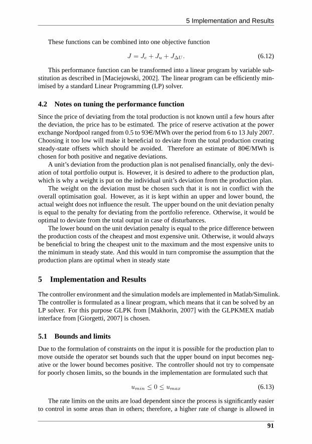
5 Implementation and Results
These functions can be combined into one objective function
J = Je + Ju + J∆U . (6.12)
This performance function can be transformed into a linear program by variable sub-stitution as described in [Maciejowski, 2002]. The linear program can be efficiently min-imised by a standard Linear Programming (LP) solver.
4.2 Notes on tuning the performance function
Since the price of deviating from the total production is notknown until a few hours afterthe deviation, the price has to be estimated. The price of reserve activation at the powerexchange Nordpool ranged from 0.5 to 93e/MWh over the period from 6 to 13 July 2007.Choosing it too low will make it beneficial to deviate from thetotal production creatingsteady-state offsets which should be avoided. Therefore anestimate of 80e/MWh ischosen for both positive and negative deviations.
A unit’s deviation from the production plan is not penalisedfinancially, only the devi-ation of total portfolio output is. However, it is desired toadhere to the production plan,which is why a weight is put on the individual unit’s deviation from the production plan.
The weight on the deviation must be chosen such that it is not in conflict with theoverall optimisation goal. However, as it is kept within an upper and lower bound, theactual weight does not influence the result. The upper bound on the unit deviation penaltyis equal to the penalty for deviating from the portfolio reference. Otherwise, it would beoptimal to deviate from the total output in case of disturbances.
The lower bound on the unit deviation penalty is equal to the price difference betweenthe production costs of the cheapest and most expensive unit. Otherwise, it would alwaysbe beneficial to bring the cheapest unit to the maximum and themost expensive units tothe minimum in steady state. And this would in turn compromise the assumption that theproduction plans are optimal when in steady state
5 Implementation and Results
The controller environment and the simulation models are implemented in Matlab/Simulink.The controller is formulated as a linear program, which means that it can be solved by anLP solver. For this purpose GLPK from [Makhorin, 2007] with the GLPKMEX matlabinterface from [Giorgetti, 2007] is chosen.
5.1 Bounds and limits
Due to the formulation of constraints on the input it is possible for the production plan tomove outside the operator set bounds such that the upper bound on input becomes neg-ative or the lower bound becomes positive. The controller should not try to compensatefor poorly chosen limits, so the bounds in the implementation are formulated such that
umin ≤ 0 ≤ umax (6.13)
The rate limits on the units are load dependent since the process is significantly easierto control in some areas than in others; therefore, a higher rate of change is allowed in
91
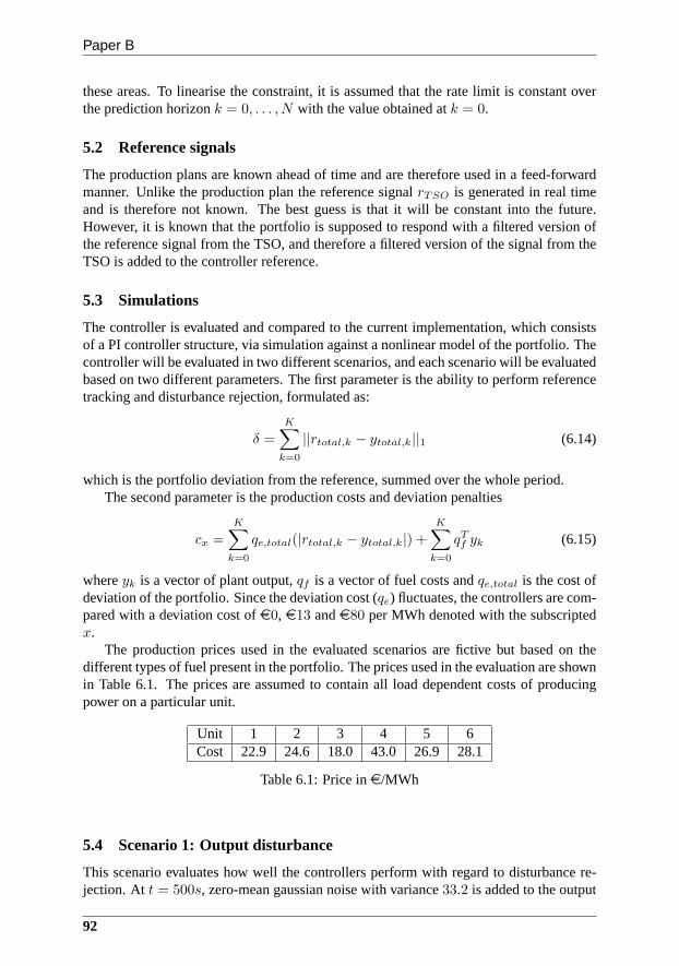
Paper B
these areas. To linearise the constraint, it is assumed thatthe rate limit is constant overthe prediction horizonk = 0, . . . , N with the value obtained atk = 0.
5.2 Reference signals
The production plans are known ahead of time and are therefore used in a feed-forwardmanner. Unlike the production plan the reference signalrTSO is generated in real timeand is therefore not known. The best guess is that it will be constant into the future.However, it is known that the portfolio is supposed to respond with a filtered version ofthe reference signal from the TSO, and therefore a filtered version of the signal from theTSO is added to the controller reference.
5.3 Simulations
The controller is evaluated and compared to the current implementation, which consistsof a PI controller structure, via simulation against a nonlinear model of the portfolio. Thecontroller will be evaluated in two different scenarios, and each scenario will be evaluatedbased on two different parameters. The first parameter is theability to perform referencetracking and disturbance rejection, formulated as:
δ =
K∑
k=0
||rtotal,k − ytotal,k||1 (6.14)
which is the portfolio deviation from the reference, summedover the whole period.The second parameter is the production costs and deviation penalties
cx =
K∑
k=0
qe,total(|rtotal,k − ytotal,k|) +
K∑
k=0
qTf yk (6.15)
whereyk is a vector of plant output,qf is a vector of fuel costs andqe,total is the cost ofdeviation of the portfolio. Since the deviation cost (qe) fluctuates, the controllers are com-pared with a deviation cost ofe0, e13 ande80 per MWh denoted with the subscriptedx.
The production prices used in the evaluated scenarios are fictive but based on thedifferent types of fuel present in the portfolio. The pricesused in the evaluation are shownin Table 6.1. The prices are assumed to contain all load dependent costs of producingpower on a particular unit.
Unit 1 2 3 4 5 6Cost 22.9 24.6 18.0 43.0 26.9 28.1
Table 6.1: Price ine/MWh
5.4 Scenario 1: Output disturbance
This scenario evaluates how well the controllers perform with regard to disturbance re-jection. At t = 500s, zero-mean gaussian noise with variance33.2 is added to the output
92
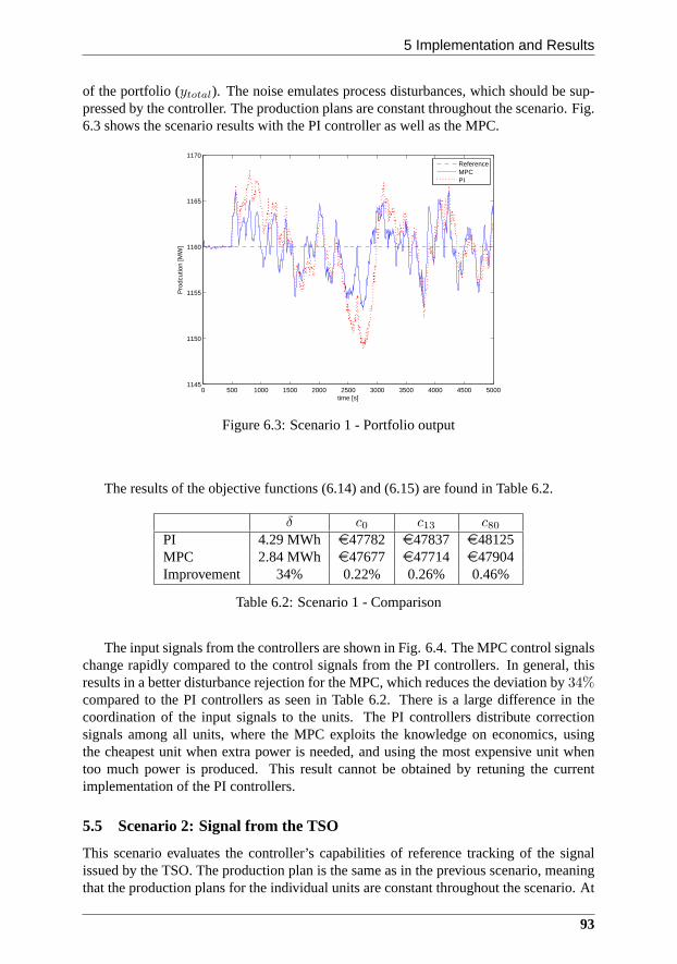
5 Implementation and Results
of the portfolio (ytotal). The noise emulates process disturbances, which should besup-pressed by the controller. The production plans are constant throughout the scenario. Fig.6.3 shows the scenario results with the PI controller as wellas the MPC.
0 500 1000 1500 2000 2500 3000 3500 4000 4500 50001145
1150
1155
1160
1165
1170
time [s]
Pro
dcut
ion
[MW
]
ReferenceMPCPI
Figure 6.3: Scenario 1 - Portfolio output
The results of the objective functions (6.14) and (6.15) arefound in Table 6.2.
δ c0 c13 c80PI 4.29 MWh e47782 e47837 e48125MPC 2.84 MWh e47677 e47714 e47904Improvement 34% 0.22% 0.26% 0.46%
Table 6.2: Scenario 1 - Comparison
The input signals from the controllers are shown in Fig. 6.4.The MPC control signalschange rapidly compared to the control signals from the PI controllers. In general, thisresults in a better disturbance rejection for the MPC, whichreduces the deviation by34%compared to the PI controllers as seen in Table 6.2. There is alarge difference in thecoordination of the input signals to the units. The PI controllers distribute correctionsignals among all units, where the MPC exploits the knowledge on economics, usingthe cheapest unit when extra power is needed, and using the most expensive unit whentoo much power is produced. This result cannot be obtained byretuning the currentimplementation of the PI controllers.
5.5 Scenario 2: Signal from the TSO
This scenario evaluates the controller’s capabilities of reference tracking of the signalissued by the TSO. The production plan is the same as in the previous scenario, meaningthat the production plans for the individual units are constant throughout the scenario. At
93
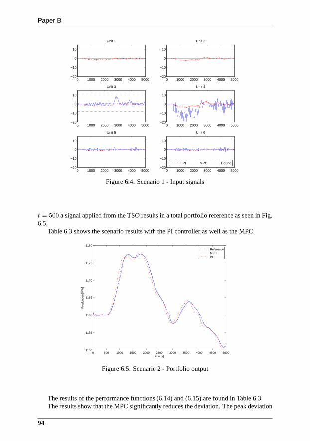
Paper B
0 1000 2000 3000 4000 5000−20
−10
0
10
Unit 1
0 1000 2000 3000 4000 5000−20
−10
0
10
Unit 2
0 1000 2000 3000 4000 5000−20
−10
0
10
Unit 3
0 1000 2000 3000 4000 5000−20
−10
0
10
Unit 4
0 1000 2000 3000 4000 5000−20
−10
0
10
Unit 5
0 1000 2000 3000 4000 5000−20
−10
0
10
Unit 6
PI MPC Bound
Figure 6.4: Scenario 1 - Input signals
t = 500 a signal applied from the TSO results in a total portfolio reference as seen in Fig.6.5.
Table 6.3 shows the scenario results with the PI controller as well as the MPC.
0 500 1000 1500 2000 2500 3000 3500 4000 4500 50001150
1155
1160
1165
1170
1175
1180
time [s]
Pro
dcut
ion
[MW
]
ReferenceMPCPI
Figure 6.5: Scenario 2 - Portfolio output
The results of the performance functions (6.14) and (6.15) are found in Table 6.3.The results show that the MPC significantly reduces the deviation. The peak deviation
94
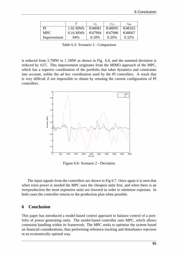
6 Conclusion
δ c0 c13 c80PI 1.02 MWh e48081 e48095 e48163MPC 0.16 MWh e47994 e47996 e48007Improvement 84% 0.18% 0.20% 0.32%
Table 6.3: Scenario 2 - Comparison
is reduced from2.7MW to 1.1MW as shown in Fig. 6.6, and the summed deviation isreduced by84%. This improvement originates from the MIMO approach of the MPC,which has a superior coordination of the portfolio that takes dynamics and constraintsinto account, unlike the ad hoc coordination used by the PI controllers. A result thatis very difficult if not impossible to obtain by retuning the current configuration of PIcontrollers.
0 500 1000 1500 2000 2500 3000 3500 4000 4500 5000−2
−1.5
−1
−0.5
0
0.5
1
1.5
2
2.5
3
time [s]
Dev
iatio
n [M
W]
MPCPI
Figure 6.6: Scenario 2 - Deviation
The input signals from the controllers are shown in Fig 6.7. Once again it is seen thatwhen extra power is needed the MPC uses the cheapest units first, and when there is anoverproduction the most expensive units are lowered in order to minimise expenses. Inboth cases the controller returns to the production plan when possible.
6 Conclusion
This paper has introduced a model-based control approach tobalance control of a port-folio of power generating units. The model-based controller uses MPC, which allowsconstraint handling within its framework. The MPC seeks to optimise the system basedon financial considerations, thus performing reference tracking and disturbance rejectionin an economically optimal way.
95
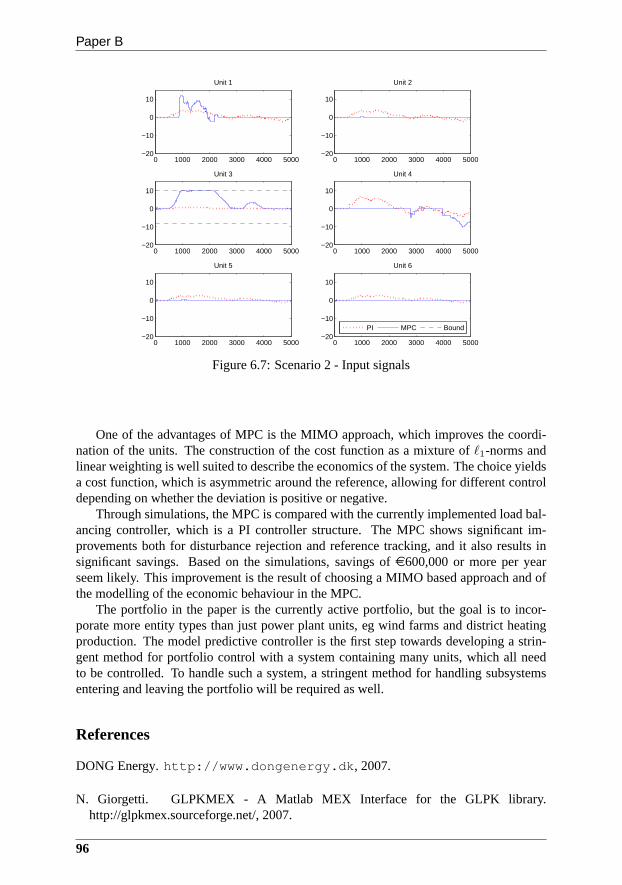
Paper B
0 1000 2000 3000 4000 5000−20
−10
0
10
Unit 1
0 1000 2000 3000 4000 5000−20
−10
0
10
Unit 2
0 1000 2000 3000 4000 5000−20
−10
0
10
Unit 3
0 1000 2000 3000 4000 5000−20
−10
0
10
Unit 4
0 1000 2000 3000 4000 5000−20
−10
0
10
Unit 5
0 1000 2000 3000 4000 5000−20
−10
0
10
Unit 6
PI MPC Bound
Figure 6.7: Scenario 2 - Input signals
One of the advantages of MPC is the MIMO approach, which improves the coordi-nation of the units. The construction of the cost function asa mixture ofℓ1-norms andlinear weighting is well suited to describe the economics ofthe system. The choice yieldsa cost function, which is asymmetric around the reference, allowing for different controldepending on whether the deviation is positive or negative.
Through simulations, the MPC is compared with the currentlyimplemented load bal-ancing controller, which is a PI controller structure. The MPC shows significant im-provements both for disturbance rejection and reference tracking, and it also results insignificant savings. Based on the simulations, savings ofe600,000 or more per yearseem likely. This improvement is the result of choosing a MIMO based approach and ofthe modelling of the economic behaviour in the MPC.
The portfolio in the paper is the currently active portfolio, but the goal is to incor-porate more entity types than just power plant units, eg windfarms and district heatingproduction. The model predictive controller is the first step towards developing a strin-gent method for portfolio control with a system containing many units, which all needto be controlled. To handle such a system, a stringent methodfor handling subsystemsentering and leaving the portfolio will be required as well.
References
DONG Energy.http://www.dongenergy.dk, 2007.
N. Giorgetti. GLPKMEX - A Matlab MEX Interface for the GLPK library.http://glpkmex.sourceforge.net/, 2007.
96
6 Conclusion
C. Jørgensen, J. H. Mortensen, T. Mølbak, and E. O. Nielsen. Modelbased Fleet Opti-mization and Master Control of a Power Production System. InProceedings of IFACSymposium on Power Plants and Power Systems Control 2006, Kananaskis, Canada,2006.
G. K. Lausterer. Improved maneuverability of power plants for better grid stability.Con-trol Engineering Practice, 6(12):1549–1557, 1998.
J. M. Maciejowski. Predictive Control with Constraints. Pearson Education Limited,2002. ISBN 0-201-39823-0.
A. Makhorin. Gnu Linear Programming Kit - GLPK. http://www.gnu.org/software/glpk/,2007.
UCTE. European Wind Integration Study (EWIS) Towards a successful integration ofwind power into european electricity grids. Technical report, UCTE, 2007.
E. Welfonder. Least-cost dynamic interaction of power plants and power systems.ControlEngineering Practice, 5(9):1203–1216, 1997.
97

Paper C
Simple Models for Model-based Portfolio Load Balancing ControllerSynthesis
Kristian Edlund, Jan Dimon Bendtsen & Tommy Mølbak
This paper was published in:Proceedings of IFAC Symposium on power plants and power systems control
2009

Copyright c©International Federation of Automatic ControlThe layout has been revised

1 Introduction
Abstract
This paper presents a collection of models of so-called ’effectuators’,i.e., subsys-tems in a power plant portfolio that represent control actions with associated dynam-ics and actuation costs. These models are derived in order to facilitate higher-levelmodel-based control synthesis of a portfolio of generation units existing inan electri-cal power supply network, for instance in model-based predictive control or declara-tive control schemes. We focus on the effectuators found in the Danishpower system.In particular, the paper presents models for boiler load, district heating,condensatethrottling and wind turbine effectuators. Each model is validated against actual mea-surement data. Considering their simplicity, the models fit the observed data verywell and are thus suitable for control purposes.
1 Introduction
Currently a large part of the world is deeply concerned aboutglobal warming and theconsequences that might follow from emission of green housegases. This has amongother things led to the signing of the Kyoto Protocol [UnitedNations, 1998]. ThroughoutEurope, this has given use to a very ambitious project to increase the share of energydelivered by renewable sources such as wind [UCTE, 2007]. InDenmark the goal is toincrease the share of electrical energy coming from renewable sources from 24% in 2005to 36% in 2025 as found in [Danish Ministry of Transport and Energy, 2005].
Due to the geography of Denmark much of this renewable energyhas to come fromwind turbines. Given the stochastic behaviour of the wind turbines, a flexible powersystem and good load balancing control is needed, in order toavoid blackouts.
DONG Energy owns and operates a portfolio of power plants in Western Denmarkas shown in Fig. 7.1. With respect to the communication with the Transmission SystemOperator (TSO), this portfolio is considered as one entity both regarding deviations andactivation of reserves. To accommodate this, DONG Energy has created a load balanc-ing controller to minimise the deviation of the portfolio from the reference as well asdistribute the ordered reserve activation.
In [Edlund et al., 2008] we showed through simulations that it was possible to sig-nificantly decrease the deviation between the portfolio output and the reference by intro-ducing a model-based control scheme for the balance controller. The focus was to showthat it is possible to gain better economics and decrease thedeviation, and only little at-tention was paid to the models used in the control scheme. In this paper we focus on themodels of the generation units. A control strategy for how tocoordinate the individualeffectuators is not discussed in this paper.
In the existing literature there are many detailed models ofparts of the energy sys-tem, used to describe the dynamic behaviour of individual system components, such as[de Mello, 1991; Weber and Krueger, 2008; Welfonder, 1997].However, the aim in thispaper is to construct simple models which are suitable for controller synthesis of a model-based control scheme for load balancing control.
There are many ways to manipulate the output from the portfolio to follow the refer-ences. Here we shall use the termeffectuatoras a unifying term for all of them.
101
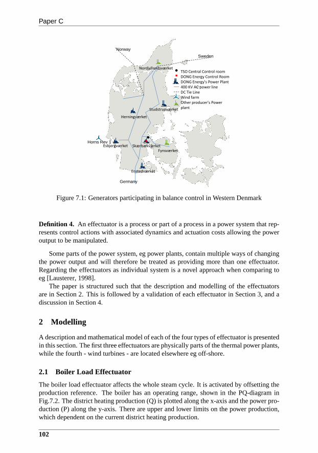
Paper C
Studstrupværket
Herningværket
DONG Energy's Power Plant
DONG Energy Control Room
TSO Central Control room
Horns Rev 1
400 KV AC power line
DC Tie Line
Wind farm
Nordjyllandsværket
Other producer's Power
plant
Norway
Sweden
Esbjergværket Skærbækværket
Enstedværket
Horns Rev 1
Fynsværket
Germany
Figure 7.1: Generators participating in balance control inWestern Denmark
Definition 4. An effectuator is a process or part of a process in a power system that rep-resents control actions with associated dynamics and actuation costs allowing the poweroutput to be manipulated.
Some parts of the power system, eg power plants, contain multiple ways of changingthe power output and will therefore be treated as providing more than one effectuator.Regarding the effectuators as individual system is a novel approach when comparing toeg [Lausterer, 1998].
The paper is structured such that the description and modelling of the effectuatorsare in Section 2. This is followed by a validation of each effectuator in Section 3, and adiscussion in Section 4.
2 Modelling
A description and mathematical model of each of the four types of effectuator is presentedin this section. The first three effectuators are physicallyparts of the thermal power plants,while the fourth - wind turbines - are located elsewhere eg off-shore.
2.1 Boiler Load Effectuator
The boiler load effectuator affects the whole steam cycle. It is activated by offsetting theproduction reference. The boiler has an operating range, shown in the PQ-diagram inFig.7.2. The district heating production (Q) is plotted along the x-axis and the power pro-duction (P) along the y-axis. There are upper and lower limits on the power production,which dependent on the current district heating production.
102

2 Modelling
P[MW]
Q [MJ/S]
Operating point
Figure 7.2: Movement in the PQ-diagram when changing the boiler load
When using the boiler for control purposes the district heating production is main-tained, meaning that the changes in production happens vertically in the PQ-diagram asshown in Fig. 7.2.
This effectuator is slow in a load balancing context (minutes), but the potential energyproduction is unlimited, meaning that the corrections can be maintained by this effectua-tor for an unlimited time period. There is a large amount of power available in this typeof effectuator.
Besides the behaviour of the boiler, there is a communication delay between the loadbalancing controller and the power plant. However, this delay is so small compared to thedynamics that it can be neglected for this effectuator.
Effectuator Model
There are two communication methods for activating the boiler load effectuator in a powerplant, either through the production plan or through an input used by the balance con-troller to give real time corrections to the boiler load effectuator. The production plan isnot controllable and is therefore modelled as a disturbance. The output of the model isthe produced power from the unit caused by the boiler load effectuator.
The model is formulated as a greybox model and the dynamics are assumed to beadequately described as the following state space system
xb =
−T−1b 0 0
T−1b −T−1
b 00 T−1
b −T−1b
xb +
T−1b
00
u+
T−1b
00
d
y =[
0 0 1]
xb. (7.1)
whereTb is the time constant for the effectuator.u is the input given by the balancecontroller,d is the production plan and additional manually ordered corrections.
Upper and Lower limits
The limits can be set by the operator, or can be given by the process. The limits are appliedto the input such thatP b ≤ u ≤ P b. It is assumed that the upper limit is non-negativeand the lower limit is non-positive.
103
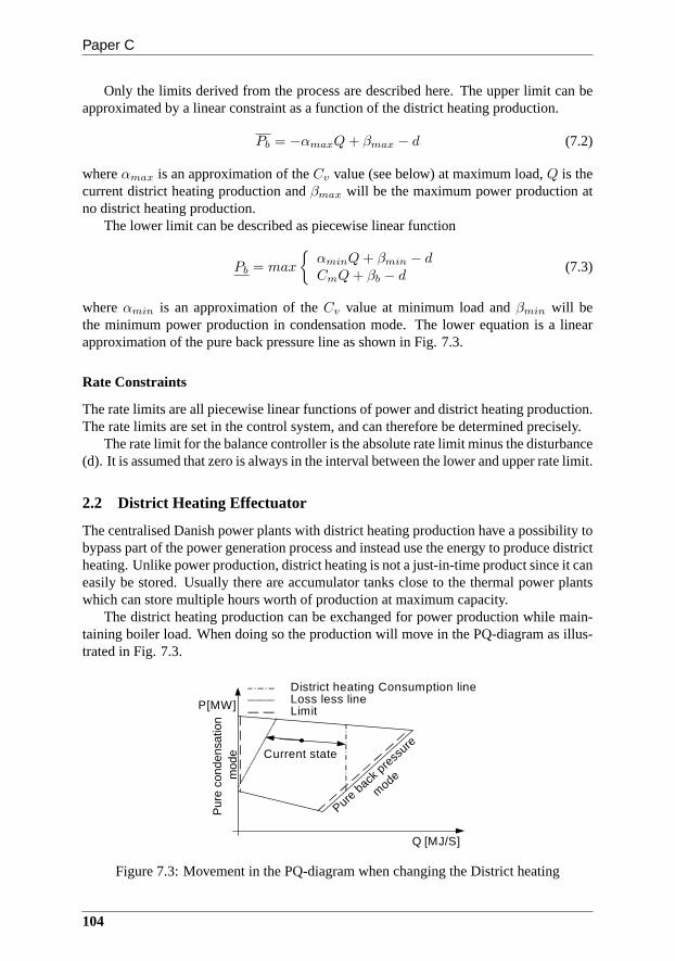
Paper C
Only the limits derived from the process are described here.The upper limit can beapproximated by a linear constraint as a function of the district heating production.
Pb = −αmaxQ+ βmax − d (7.2)
whereαmax is an approximation of theCv value (see below) at maximum load,Q is thecurrent district heating production andβmax will be the maximum power production atno district heating production.
The lower limit can be described as piecewise linear function
Pb = max
{
αminQ+ βmin − dCmQ+ βb − d
(7.3)
whereαmin is an approximation of theCv value at minimum load andβmin will bethe minimum power production in condensation mode. The lower equation is a linearapproximation of the pure back pressure line as shown in Fig.7.3.
Rate Constraints
The rate limits are all piecewise linear functions of power and district heating production.The rate limits are set in the control system, and can therefore be determined precisely.
The rate limit for the balance controller is the absolute rate limit minus the disturbance(d). It is assumed that zero is always in the interval betweenthe lower and upper rate limit.
2.2 District Heating Effectuator
The centralised Danish power plants with district heating production have a possibility tobypass part of the power generation process and instead use the energy to produce districtheating. Unlike power production, district heating is not ajust-in-time product since it caneasily be stored. Usually there are accumulator tanks closeto the thermal power plantswhich can store multiple hours worth of production at maximum capacity.
The district heating production can be exchanged for power production while main-taining boiler load. When doing so the production will move inthe PQ-diagram as illus-trated in Fig. 7.3.
P[MW]
Q [MJ/S]
Current state
Pur
e co
nden
satio
n m
ode
Pure b
ack p
ress
ure
mode
Loss less lineDistrict heating Consumption line
Limit
Figure 7.3: Movement in the PQ-diagram when changing the District heating
104
2 Modelling
The loss of steam for power production is highly dependent onthe state of the unit.Lowering the power output with1MW will typically increase the district heating produc-tion with 2-7 MW. The exchange factor is called theCv-value and is a nonlinear functionof the boiler load, typically the function is in the range0.1− 0.4.
When used as an effectuator, there are several constraints which should not be vio-lated, since it results in changes in the physical process. Fig. 7.3 shows an example ofsuch a constraint the district heating consumption line. Crossing the consumption linemeans that the accumulator tank goes from charging to discharging, and that requires alarge discrete change in the physical process.
The district heating effectuator is characterised as a medium fast effectuator (approx.30 sec). The potential energy is limited due to the accumulator tanks. The potential powerthat can be drawn from this effectuator is big, but it is stillsmaller than the power in theboiler load effectuator.
Besides the behaviour of the district heating system, thereis a communication delaybetween the load balancing controller and the power plant.
Effectuator Model
The desired input to the model is a reference to the power output, and the desired outputis the actual power production from the effectuator. The model constructed here is anonlinear model.
The change in district heating is modeled as a first order linear system with a timedelay. The time constant in the system is typically around30s while the communicationdelaytd is a result of interacting computer systems communicating over a network withno real time guarantees. The delay is therefore treated as being stochastic, but it typicallyranges between5 and10 seconds. To convert the system so the output is power productionthe input and output values are multiplied and divided byCv, thus yielding a nonlinearstate space model.
xdh(t) = −1
30xdh(t) +
1
30Cv
u(t− td) (7.4)
y(t) = −Cvxdh(t).
Upper and Lower Limits
This model will only include limits for the charging lines and the plants physical limita-tions, such as a minimum production of no district heating.
The limits are implemented in the local control system so it is reasonable to apply thelimits to the input of the model. The input to the effectuatorshould be within the limitsPdh ≤ u ≤ Pdh, and it is assumed that0 is always a valid solution for the inequality.
The upper limit is given as the minimum of two constraints
Pdh = min
{
CvQplan
Cv(Qplan −Qconsump)(7.5)
whereQplan is the production plan for district heating, andQconsump is the district heat-ing consumption. The lower constraint is only active if the unit is charging the accumu-lator tank
105

Paper C
The minimum limit is given by the back pressure line. The equivalent condensationmode production corresponding to the current load is found as
Pcon = CvQ+ P (7.6)
The distance between the district heating plan and a a linearapproximation of the backpressure line as a function ofPcon is used to find the maximum district heating productionpossible at that load. Thus the minimum power correction is found as
Pdh = min
{
−Cv(αbackPcon + βback −Qplan)Cv(Qplan −Qconsump)
(7.7)
The lower constraint is only active if the unit is discharging the accumulator tank.
Rate Constraints
There are rate limits on how fast the district heating production can be changed, whichmeans that the changes from the district heating effectuator plus the district heating pro-duction should not be changes faster than a given limit. Thislimit is assumed constantthroughout the whole state space. The rate limits can be expressed as
∆Pdh = α∆dhCv (7.8)
whereα∆dh is the district heating production rate of change constraint constant. Thelimit is typically 30 − 50MJ/s/min, which with a typicalCv value of0.2 gives a ratelimit of 6− 10MW/min in the power production.
2.3 Condensate Throttling Effectuator
The condensate system is the system that preheats the condensate and transports it fromthe condenser to the feedwater tank.
An example of a condensate system is depicted in Fig. 7.4. By changing the conden-sate flow, the steam demand can be changed and thereby affect the power output quickly.For more details on this effectuator see [Lausterer, 1998] as well as [Welfonder, 1997],where the authors also propose to use this effectuator to control the power output fromthe power plant unit.
Cooling water
From turbine outlets
Feed water tank
From district heating
Condensed steam
Figure 7.4: Example of a condensate System
The nominal flow in the condensate system varies with the boiler load, therefore en-ergy and power limits varies as a function of this. At all times neither the condenser nor
106
2 Modelling
the feed water tank should be completely emptied or filled. This means that the effectuatorcan deliver a limited amount of energy.
There is typically very little energy stored in the condensate throttling system, so itcan only be used for a few minutes to manipulate the power production. On the otherhand it reacts in a matter of seconds. The available power is in general much smaller thanthe energy the available power in the boiler load effectuator.
Besides the behaviour of the condensate system, there is a communication delay be-tween the load balancing controller and the power plant.
Effectuator Model
The dynamics of the system from reference to power output canbe approximated by alineaer low-pass filter and a time delay. The time constant is20 seconds for the whole op-erating range. The time delay is equal to the one found in the district heating effectuator.
The ratio between flow and power is a nonlinear functionf(P,Q) dependent on thepower and district heating production.
The model of the system can be put in the form of a parameter varying state spacesystem.
xc =
[
−1/20 0f(P,Q) 0
]
xc(t) +
[
1/200
]
u(t− td) (7.9)
y =
[
1 00 1
]
xc(t). (7.10)
The output from the statespace model is
y =
[
P (MW )V (m3)
]
(7.11)
where the first term is the current power output from the system, and the second term isthe water volume displaced from the setpoint of the tank. Themodel is valid as long asthe states are kept within the described bounds.
Upper and Lower Limits
The limits are described in the control system as a piecewiselinear function dependenton the current power and district heating production.
It is assumed that the condenser and tank where the district heating condensate entersthe condensate system are balanced, such that the flow between condenser and feedwatertank is coordinated according to the flow entering from the district heating. The systemconsists of three tanks, where the water is moved between, but it will be modelled as onetank, where it is possible pour water into, or drain water. Aslong as the level is keptwithin certain bounds. These level bounds in this one virtual tank, originates from themost restricting of the three tanks for upper and lower bounds.
The limits of the volume used in the model are defined as
V c = min
V cond − V0,cond
V lph4 − V0,lph4
V0,fwt − V fwt
V c = min
V cond − V0,cond
V lph4 − V0,lph4
V0,fwt − V fwt
(7.12)
107
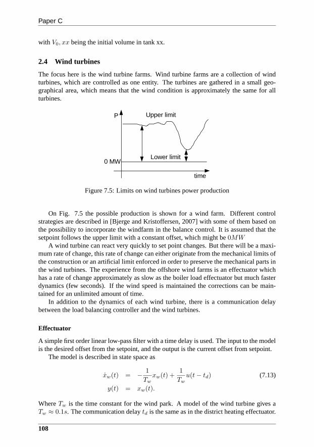
Paper C
with V0, xx being the initial volume in tank xx.
2.4 Wind turbines
The focus here is the wind turbine farms. Wind turbine farms are a collection of windturbines, which are controlled as one entity. The turbines are gathered in a small geo-graphical area, which means that the wind condition is approximately the same for allturbines.
time
P
0 MW
Upper limit
Lower limit
Figure 7.5: Limits on wind turbines power production
On Fig. 7.5 the possible production is shown for a wind farm. Different controlstrategies are described in [Bjerge and Kristoffersen, 2007] with some of them based onthe possibility to incorporate the windfarm in the balance control. It is assumed that thesetpoint follows the upper limit with a constant offset, which might be0MW
A wind turbine can react very quickly to set point changes. But there will be a maxi-mum rate of change, this rate of change can either originate from the mechanical limits ofthe construction or an artificial limit enforced in order to preserve the mechanical parts inthe wind turbines. The experience from the offshore wind farms is an effectuator whichhas a rate of change approximately as slow as the boiler load effectuator but much fasterdynamics (few seconds). If the wind speed is maintained the corrections can be main-tained for an unlimited amount of time.
In addition to the dynamics of each wind turbine, there is a communication delaybetween the load balancing controller and the wind turbines.
Effectuator
A simple first order linear low-pass filter with a time delay isused. The input to the modelis the desired offset from the setpoint, and the output is thecurrent offset from setpoint.
The model is described in state space as
xw(t) = −1
Tw
xw(t) +1
Tw
u(t− td) (7.13)
y(t) = xw(t).
WhereTw is the time constant for the wind park. A model of the wind turbine gives aTw ≈ 0.1s. The communication delaytd is the same as in the district heating effectuator.
108

3 Verification
Limits
The upper limit is given by the distance from the setpoint to the upper limit, which is setby the operator. The negative correction is bounded by zero.
Rate Limits
The described rate limit is applied to the input of the model.This yields the followingrate limits
−∆uw ≤ ∆u ≤ ∆uw (7.14)
whereu is the input to the model.
3 Verification
The models consist of both a dynamic part, and a constraint set. The constraints are eitherfound and verified using a static tool such as Turabs [Johansen, 2004], or derived fromthe implementation in the control system. The parameters inthe model are estimated byhand.
3.1 Boiler Load Effectuator
The models are likely going to be used in a predictive controlscheme. However since theprediction horizon of the scheme is unknown it is chosen to evaulate the models open-loopperformance.
0 1 2 3 440
60
80
100
120
140
Time [hours]
Pow
er O
utpu
t [M
W]
Actual outputSimulation
Figure 7.6: Verification of the dynamics of the power plant, scenario 1. The solid lineshows the actual output, and the dashed line shows the open-loop simulation
Fig. 7.6 shows the first evaluation scenario. The model is a little offset from the actualoutput. This is most likely caused by the measurements used for model validation being
109
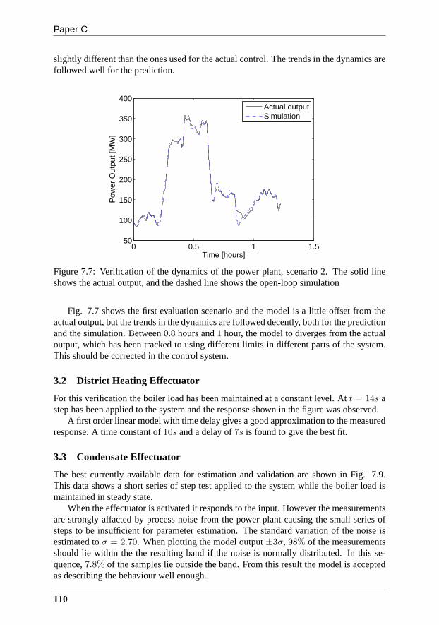
Paper C
slightly different than the ones used for the actual control. The trends in the dynamics arefollowed well for the prediction.
0 0.5 1 1.550
100
150
200
250
300
350
400
Time [hours]
Pow
er O
utpu
t [M
W]
Actual outputSimulation
Figure 7.7: Verification of the dynamics of the power plant, scenario 2. The solid lineshows the actual output, and the dashed line shows the open-loop simulation
Fig. 7.7 shows the first evaluation scenario and the model is alittle offset from theactual output, but the trends in the dynamics are followed decently, both for the predictionand the simulation. Between 0.8 hours and 1 hour, the model todiverges from the actualoutput, which has been tracked to using different limits in different parts of the system.This should be corrected in the control system.
3.2 District Heating Effectuator
For this verification the boiler load has been maintained at aconstant level. Att = 14s astep has been applied to the system and the response shown in the figure was observed.
A first order linear model with time delay gives a good approximation to the measuredresponse. A time constant of10s and a delay of7s is found to give the best fit.
3.3 Condensate Effectuator
The best currently available data for estimation and validation are shown in Fig. 7.9.This data shows a short series of step test applied to the system while the boiler load ismaintained in steady state.
When the effectuator is activated it responds to the input. However the measurementsare strongly affacted by process noise from the power plant causing the small series ofsteps to be insufficient for parameter estimation. The standard variation of the noise isestimated toσ = 2.70. When plotting the model output±3σ, 98% of the measurementsshould lie within the the resulting band if the noise is normally distributed. In this se-quence,7.8% of the samples lie outside the band. From this result the model is acceptedas describing the behaviour well enough.
110
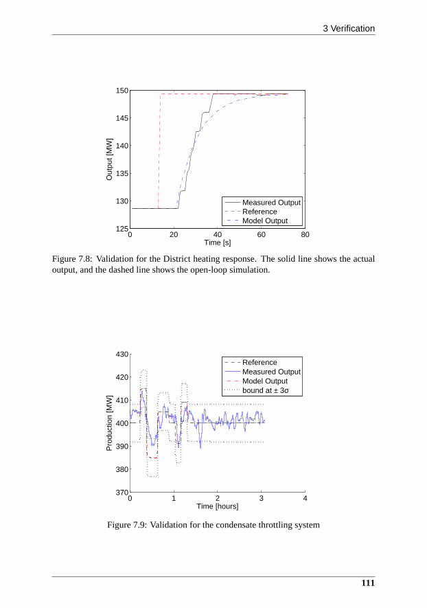
3 Verification
0 20 40 60 80125
130
135
140
145
150
Time [s]
Out
put [
MW
]
Measured OutputReferenceModel Output
Figure 7.8: Validation for the District heating response. The solid line shows the actualoutput, and the dashed line shows the open-loop simulation.
0 1 2 3 4370
380
390
400
410
420
430
Time [hours]
Pro
duct
ion
[MW
]
ReferenceMeasured OutputModel Outputbound at ± 3σ
Figure 7.9: Validation for the condensate throttling system
111
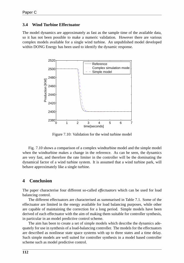
Paper C
3.4 Wind Turbine Effectuator
The model dynamics are approximately as fast as the sample time of the available data,so it has not been possible to make a numeric validation. However there are variouscomplex models available for a single wind turbine. An unpublished model developedwithin DONG Energy has been used to identify the dynamic response.
0 1 2 3 4 5 6 72380
2400
2420
2440
2460
2480
2500
2520
time[seconds]
Pro
duct
ion
[KW
]
ReferenceComplex simulation modeSimple model
Figure 7.10: Validation for the wind turbine model
Fig. 7.10 shows a comparison of a complex windturbine model and the simple modelwhen the windturbine makes a change in the reference. As can be seen, the dynamicsare very fast, and therefore the rate limiter in the controller will be the dominating thedynamical factor of a wind turbine system. It is assumed thata wind turbine park, willbehave approximately like a single turbine.
4 Conclusion
The paper characterise four different so-calledeffectuatorswhich can be used for loadbalancing control.
The different effectuators are characterised as summarised in Table 7.1. Some of theeffectuator are limited in the energy available for load balancing purposes, while otherare capable of maintaining the correction for a long period.Simple models have beenderived of each effectuator with the aim of making them suitable for controller synthesis,in particular in an model predictive control scheme.
The aim has been to create a set of simple models which describe the dynamics ade-quately for use in synthesis of a load-balancing controller. The models for the effectuatorsare described as nonlinear state space systems with up to three states and a time delay.Such simple models are well suited for controller synthesisin a model based controllerscheme such as model predictive control.
112

4 Conclusion
effectuator Energy Power DynamicsBoiler load Unlimited Large > 1minDistrict heating Large Medium 20− 40sCondensate throttling Small Medium 10− 15sWind turbines Unlimited Medium < 5s
Table 7.1: Comparison of the effectuators.
References
C. Bjerge and J. R. Kristoffersen. Run an offshore wind farm like a power plant.VGBPowertech, 87(4):63–66, 2007.
Danish Ministry of Transport and Energy. Energistrategi 2025 - Perspektiver frem mod2025. Technical report, Transport- og Energiministeriet,2005.
F. P. de Mello. Boiler models for system dynamical performance studies.IEEE Transac-tions on Power Systems, 6(1):66–74, 1991.
K. Edlund, J. D. Bendtsen, S. Børresen, and T. Mølbak. Introducing Model PredictiveControl for Improving Power Plant Portfolio Performance.Proceedings of the 17thIFAC World Congress, Seoul, South Korea, pages 6986–6991, 2008.
A. O. Johansen. Simulation and optimisation of thermal power stations by use of Turabs.Technical report, DONG Energy, 2004.
G. K. Lausterer. Improved maneuverability of power plants for better grid stability.Con-trol Engineering Practice, 6(12):1549–1557, 1998.
UCTE. European Wind Integration Study (EWIS) Towards a successful integration ofwind power into european electricity grids. Technical report, UCTE, 2007.
United Nations. Kyoto protocol to the United Nations framework convention on climatechange. Technical report, United Nations, 1998.
H. Weber and M. Krueger. Dynamic investigation of network restoration by the pumped-storage plant Markersbach in Germany.Proceedings of the 17th IFAC World Congress,Seoul, Korea, 2008.
E. Welfonder. Least-cost dynamic interaction of power plants and power systems.ControlEngineering Practice, 5(9):1203–1216, 1997.
113

Paper D
A Primal-Dual Interior-Point Linear Programming Algorithm forMPC
Kristian Edlund, Leo Emil Sokoler & John Bagterp Jørgensen
This paper was published in:Proceedings of 48th IEEE Conference on Decision and Control

Copyright c©IEEEThe layout has been revised
1 Introduction
Abstract
Constrained optimal control problems for linear systems with linear constraintsand an objective function consisting of linear andl1-norm terms can be expressedas linear programs. We develop an efficient primal-dual interior point algorithm forsolution of such linear programs. The algorithm is implemented in Matlab and itsperformance is compared to an active set based LP solver and linprogin Matlab’soptimization toolbox. Simulations demonstrate that the new algorithm is more thanone magnitude faster than the other LP algorithms applied to this problem.
1 Introduction
In MPC applications, the performance and reliability of theoptimization algorithm solv-ing the constrained optimal control problem is important asthe optimization problemis solved repeatedly online. In this paper we develop a primal-dual interior-point algo-rithm for model predictive control (MPC) with input and input-rate constraints and anobjective function consisting of linear stage costs as wellasl1-norms penalizing devia-tion from target and movements Maciejowski [2002]; Boyd andVandenberghe [2004];Edlund et al. [2008]. The primal-dual interior point algorithm is based on Mehrotra’spredictor-corrector algorithm Mehrotra [1992]; Wright [1997]; Zhang [1998]; Czyzyket al. [1999]; Nocedal and Wright [2006]. Linear programs forMPC have previouslybeen considered by Morshedi et al. [1985]; Allwright and Papavasiliou [1992]; Rao andRawlings [2000]. Interior-point algorithms based on Riccati iterations for solution of anl2 constrained regulation problem Rao et al. [1998] and a robust l1 constrained regula-tion problem Vandenberghe et al. [2002] have been reported.In this paper, we use stateelimination to construct a structured linear program with upper and lower limits on thedecision variables, and highly structured general constraints. The special structure of theconstraints in this linear program is utilized by the primal-dual interior-point algorithm.
1.1 Power Portfolio Control
DONG Energy is the main power generating company in Denmark.It operates a portfolioof power plants and wind turbine farms for electricity and district heating production. Thewind turbines constitute a large share: 30% of the installedgeneration capacity in WesternDenmark. The share is expected to increase even further as a new wind turbine park isadded to the portfolio at the end of 2009. In addition a large pool of electric cars areadded to the power network.
In a liberalized electricity market, such an interconnected power and heating systemwith significant stochastic generators and consumers needsan agile and robust controlsystem to coordinate the most economic power generation respecting constraints, long-term contracts, and short-term demand-fluctuations.
By simulation Model Predictive Control has been demonstrated as a very promisingtechnology for dynamic regulation and coordination of power generation in the DONGEnergy portfolio Edlund et al. [2008]. This controller is called the DONG Energy port-folio balance controller. The controller reduces the deviation between sold and actualproduction in the most economical way. This is an example of Model Predictive Control
117
Paper D
with an economical rather than a traditional target deviation objective function Rawlingsand Amrit [2009].
The models used in this paper has been derived in Edlund et al.[2009]. To test dif-ferent optimization algorithms, and the possibility to exploit the structure of the problem,we consider a single subsystem of the entire power generation portfolio. The subsystemis a single boiler load effectuator with the simplification that rate-of-movement limits canbe specified as parameters Edlund et al. [2009].
1.2 Paper Organization
In Section 2 we state the constrained optimal control problem with a linear cost andl1-norm penalties. We derive the LP problem used to compute the solution of the constrainedoptimal control problem. Section 3 describes the interior-point algorithm for an inequalityconstrained linear program. Section 4 specializes the operations in this algorithm to theLP problem for the constrained optimal control problem withlinear cost andl1-penalties.Section 5 compares the developed interior-point algorithmfor the MPC-LP to off-the-shelf LP solvers. Section 6 concludes on the results.
2 Problem Definition
We state the control problem that is to be used in the power balance controller in con-trolling one power generating unit (a power plant). The problem and the models aredescribed in detail in Edlund et al. [2008, 2009]. The power balance controller is a ModelPredictive Controller in which a constrained optimal control problem is solved at eachsampling instant. Only the input associated to the first timeperiod is implemented andthe computations are repeated at the next sampling instant.We consider long horizons tohave economic performance as well as stability. This implies that the constrained optimalcontrol problem solved at each sampling instant is relatively large. It is important that thislarge constrained optimal control problem is solved robustly and fast as it is embedded ina real-time system.
The objective function used to measure the quality of a powertrajectory is
φ =
N−1∑
k=0
c′k+1zk+1 + ‖zk+1 − rk+1‖1,qk+1+ ‖∆uk‖1,sk
(8.1)
zk is the output (power production),rk is the reference (planned power production), anduk is the input (modified power production to meet short term fluctuations in demand).k is a time index and we consider these cost for a finite period,N = {0, 1, . . . , N − 1},characterized by the control and prediction horizon,N .
The first term represent the production costs, i.e. the cost of fuel, emission taxes etc.The second term describes the costs for deviating from the production plan computedby the production planner. The last term is a cost related to plant wear that penalizesexcessive movement of the input.
The models describing the dynamics of the system are linear.The inputs have boundand rate-of-movement constraints Edlund et al. [2009]. Therefore, the constrained opti-
118
2 Problem Definition
mal control problem solved at each sampling period is
min{uk}
N−1
k=0
φ = φ({uk}N−1k=0 ;x0, u−1, {dk,rk+1}
N−1k=0 ) (8.2a)
s.t. xk+1 = Axk +Buk + Edk k ∈ N (8.2b)
zk+1 = Cxk+1 k ∈ N (8.2c)
umin,k ≤ uk ≤ umax,k k ∈ N (8.2d)
∆umin,k ≤ ∆uk ≤ ∆umax,k k ∈ N (8.2e)
N = {0, 1, . . . , N − 1}. Note that the input bounds and the rate-of-movement constraintsare time varying.
Combination of (8.2b) and (8.2c) yields
zk = CAkx0 +k−1∑
i=0
Hu,k−iui +k−1∑
i=0
Hd,k−idi (8.3)
with k = 1, 2, ..., N and the impulse response coefficients defined in the usual way
Hu,i = CAi−1B i = 1, 2, . . . , N (8.4a)
Hd,i = CAi−1E i = 1, 2, . . . , N (8.4b)
Define the vectors
U =
u0
u1
...uN−1
D =
d0
d1
...dN−1
∆U =
∆u0
∆u1
...∆uN−1
Z =
z1z2...zN
R =
r1r2...rN
V =
v1v2...vN
W =
w1
w2
...wN
and the matrices
Φ =
CACA2
...CAN−1
Γα =
Hα,1 0 . . . 0Hα,2 Hα,1 . . . 0
......
Hα,N Hα,N−1 . . . Hα,1
with α ∈ {u, d}. Using (8.3) the stacked outputs,Z, may be expressed by the linearrelation
Z = Φx0 + ΓuU + ΓdD (8.5)
Introduce the matrices (shown for the caseN = 5)
I0 =
I0000
Ψ =
I 0 0 0 0−I I 0 0 00 −I I 0 00 0 −I I 00 0 0 −I I
119
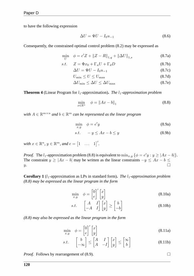
Paper D
to have the following expression
∆U = ΨU − I0u−1 (8.6)
Consequently, the constrained optimal control problem (8.2) may be expressed as
minU
φ = c′Z + ‖Z −R‖1,q + ‖∆U‖1,s (8.7a)
s.t. Z = Φx0 + ΓuU + ΓdD (8.7b)
∆U = ΨU − I0u−1 (8.7c)
Umin ≤ U ≤ Umax (8.7d)
∆Umin ≤ ∆U ≤ ∆Umax (8.7e)
Theorem 4(Linear Program forl1-approximation). Thel1-approximation problem
minx∈Rn
φ = ‖Ax− b‖1 (8.8)
withA ∈ Rm×n andb ∈ R
m can be represented as the linear program
minx,y
φ = e′y (8.9a)
s.t. − y ≤ Ax− b ≤ y (8.9b)
with x ∈ Rn, y ∈ R
m, ande =[
1 . . . 1]′
.
Proof. Thel1-approximation problem (8.8) is equivalent tominx,y {φ = e′y : y ≥ |Ax− b|}.The constrainty ≥ |Ax − b| may be written as the linear constraints−y ≤ Ax − b ≤y.
Corollary 1 (l1-approximation as LPs in standard form). Thel1-approximation problem(8.8) may be expressed as the linear program in the form
minx,y
φ =
[
0e
]′ [xy
]
(8.10a)
s.t.
[
A I−A I
] [
xy
]
≥
[
b−b
]
(8.10b)
(8.8) may also be expressed as the linear program in the form
minx,y
φ =
[
0e
]′ [xy
]
(8.11a)
s.t.
[
b−∞
]
≤
[
A IA −I
] [
xy
]
≤
[
∞b
]
(8.11b)
Proof. Follows by rearrangement of (8.9).
120

2 Problem Definition
Using Theorem 4 we may express (8.7) as
minU,V,W
φ = c′Z + s′V + q′W (8.12a)
s.t. Z = Φx0 + ΓuU + ΓdD (8.12b)
∆U = ΨU − I0u−1 (8.12c)
Umin ≤ U ≤ Umax (8.12d)
∆Umin ≤ ∆U ≤ ∆Umax (8.12e)
− V ≤ ∆U ≤ V (8.12f)
−W ≤ Z −R ≤W (8.12g)
which by elimination ofZ and ∆U is equivalent to the inequality constrained linearprogram
minU,V,W
φ = c′(Φx0 + ΓuU + ΓdD) + s′V + q′W (8.13a)
s.t. Umin ≤ U ≤ Umax (8.13b)
∆Umin ≤ ΨU − I0u−1 ≤ ∆Umax (8.13c)
− V ≤ ΨU − I0u−1 ≤ V (8.13d)
−W ≤ Φx0 + ΓuU + ΓdD −R ≤W (8.13e)
This linear program along with Corollary 1 may be used to arrive at the following linearprogram
minx
ψ = g′x (8.14a)
s.t. xl ≤ x ≤ xu (8.14b)
bl ≤ Ax ≤ bu (8.14c)
with the variables and data defined as
x =
UVW
xl =
Umin
00
xu =
Umax
∞∞
g =
gu
sq
(8.15a)
A =
Ψ 0 0Ψ I 0Ψ −I 0Γu 0 IΓu 0 −I
(8.15b)
bl =
∆Umin + I0u−1
I0u−1
−∞b−∞
bu =
∆Umax + I0u−1
∞I0u−1
∞b
(8.15c)
gu = Γ′uc (8.15d)
b = R− (Φx0 + ΓdD) (8.15e)
121
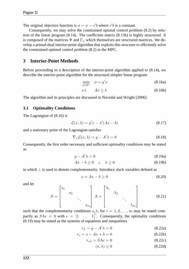
Paper D
The original objective function isφ = ψ − c′b wherec′b is a constant.Consequently, we may solve the constrained optimal controlproblem (8.2) by solu-
tion of the linear program (8.14). The coefficient matrix (8.15b) is highly structured. Itis composed of the matricesΨ andΓu which themselves are structured matrices. We de-velop a primal-dual interior-point algorithm that exploits this structure to efficiently solvethe constrained optimal control problem (8.2) in the MPC.
3 Interior-Point Methods
Before proceeding to a description of the interior-point algorithm applied to (8.14), wedescribe the interior-point algorithm for the structural simpler linear program
minx∈Rn
φ = g′x (8.16a)
s.t. Ax ≥ b (8.16b)
The algorithm and its principles are discussed in Nocedal and Wright [2006].
3.1 Optimality Conditions
The Lagrangian of (8.16) is
L(x, λ) = g′x− λ′(Ax− b) (8.17)
and a stationary point of the Lagrangian satisfies
∇xL(x, λ) = g −A′λ = 0 (8.18)
Consequently, the first order necessary and sufficient optimality conditions may be statedas
g −A′λ = 0 (8.19a)
Ax− b ≥ 0 ⊥ λ ≥ 0 (8.19b)
in which⊥ is used to denote complementarity. Introduce slack variables defined as
s = Ax− b ≥ 0 (8.20)
and let
S =
s1s2
.. .sm
Λ =
λ1
λ2
. . .λm
(8.21)
such that the complementarity conditionssiλi for i = 1, 2, . . . ,m may be stated com-pactly asSΛe = 0 with e =
[
1 . . . 1]′
. Consequently, the optimality conditions(8.19) may be stated as the systems of equations and inequalities
rL = g −A′λ = 0 (8.22a)
rs = s−Ax+ b = 0 (8.22b)
rsλ = SΛe = 0 (8.22c)
(s, λ) ≥ 0 (8.22d)
122
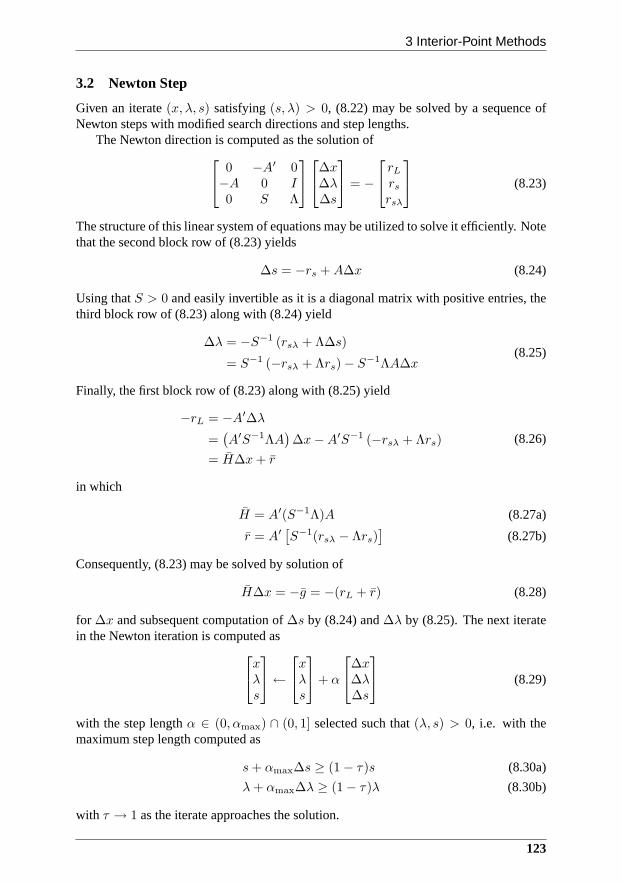
3 Interior-Point Methods
3.2 Newton Step
Given an iterate(x, λ, s) satisfying(s, λ) > 0, (8.22) may be solved by a sequence ofNewton steps with modified search directions and step lengths.
The Newton direction is computed as the solution of
0 −A′ 0−A 0 I0 S Λ
∆x∆λ∆s
= −
rLrsrsλ
(8.23)
The structure of this linear system of equations may be utilized to solve it efficiently. Notethat the second block row of (8.23) yields
∆s = −rs +A∆x (8.24)
Using thatS > 0 and easily invertible as it is a diagonal matrix with positive entries, thethird block row of (8.23) along with (8.24) yield
∆λ = −S−1 (rsλ + Λ∆s)
= S−1 (−rsλ + Λrs)− S−1ΛA∆x
(8.25)
Finally, the first block row of (8.23) along with (8.25) yield
−rL = −A′∆λ
=(
A′S−1ΛA)
∆x−A′S−1 (−rsλ + Λrs)
= H∆x+ r
(8.26)
in which
H = A′(S−1Λ)A (8.27a)
r = A′[
S−1(rsλ − Λrs)]
(8.27b)
Consequently, (8.23) may be solved by solution of
H∆x = −g = −(rL + r) (8.28)
for ∆x and subsequent computation of∆s by (8.24) and∆λ by (8.25). The next iteratein the Newton iteration is computed as
xλs
←
xλs
+ α
∆x∆λ∆s
(8.29)
with the step lengthα ∈ (0, αmax) ∩ (0, 1] selected such that(λ, s) > 0, i.e. with themaximum step length computed as
s+ αmax∆s ≥ (1− τ)s (8.30a)
λ+ αmax∆λ ≥ (1− τ)λ (8.30b)
with τ → 1 as the iterate approaches the solution.
123
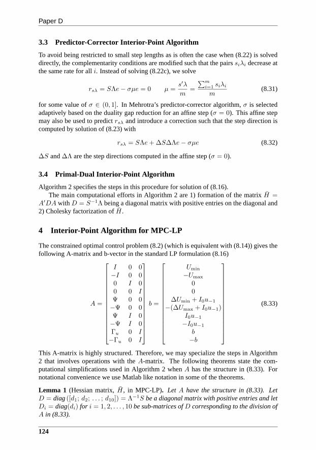
Paper D
3.3 Predictor-Corrector Interior-Point Algorithm
To avoid being restricted to small step lengths as is often the case when (8.22) is solveddirectly, the complementarity conditions are modified suchthat the pairssiλi decrease atthe same rate for alli. Instead of solving (8.22c), we solve
rsλ = SΛe− σµe = 0 µ =s′λ
m=
∑mi=1 siλi
m(8.31)
for some value ofσ ∈ (0, 1]. In Mehrotra’s predictor-corrector algorithm,σ is selectedadaptively based on the duality gap reduction for an affine step (σ = 0). This affine stepmay also be used to predictrsλ and introduce a correction such that the step direction iscomputed by solution of (8.23) with
rsλ = SΛe+ ∆S∆Λe− σµe (8.32)
∆S and∆Λ are the step directions computed in the affine step (σ = 0).
3.4 Primal-Dual Interior-Point Algorithm
Algorithm 2 specifies the steps in this procedure for solution of (8.16).The main computational efforts in Algorithm 2 are 1) formation of the matrixH =
A′DA with D = S−1Λ being a diagonal matrix with positive entries on the diagonal and2) Cholesky factorization ofH.
4 Interior-Point Algorithm for MPC-LP
The constrained optimal control problem (8.2) (which is equivalent with (8.14)) gives thefollowing A-matrix and b-vector in the standard LP formulation (8.16)
A =
I 0 0−I 0 00 I 00 0 IΨ 0 0−Ψ 0 0Ψ I 0−Ψ I 0Γu 0 I−Γu 0 I
b =
Umin
−Umax
00
∆Umin + I0u−1
−(∆Umax + I0u−1)I0u−1
−I0u−1
b−b
(8.33)
This A-matrix is highly structured. Therefore, we may specialize the steps in Algorithm2 that involves operations with theA-matrix. The following theorems state the com-putational simplifications used in Algorithm 2 whenA has the structure in (8.33). Fornotational convenience we use Matlab like notation in some of the theorems.
Lemma 1 (Hessian matrix,H, in MPC-LP). Let A have the structure in (8.33). LetD = diag([d1; d2; . . . ; d10]) = Λ−1S be a diagonal matrix with positive entries and letDi = diag(di) for i = 1, 2, . . . , 10 be sub-matrices ofD corresponding to the division ofA in (8.33).
124
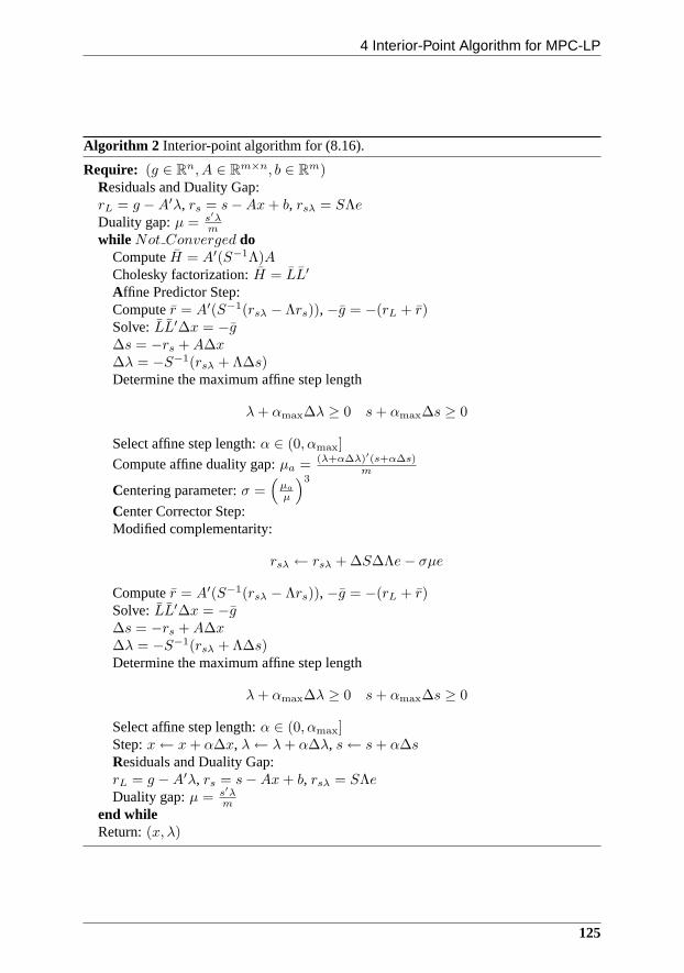
4 Interior-Point Algorithm for MPC-LP
Algorithm 2 Interior-point algorithm for (8.16).
Require: (g ∈ Rn, A ∈ R
m×n, b ∈ Rm)
Residuals and Duality Gap:rL = g −A′λ, rs = s−Ax+ b, rsλ = SΛeDuality gap:µ = s′λ
m
while Not Converged doComputeH = A′(S−1Λ)ACholesky factorization:H = LL′
Affine Predictor Step:Computer = A′(S−1(rsλ − Λrs)),−g = −(rL + r)Solve:LL′∆x = −g∆s = −rs +A∆x∆λ = −S−1(rsλ + Λ∆s)Determine the maximum affine step length
λ+ αmax∆λ ≥ 0 s+ αmax∆s ≥ 0
Select affine step length:α ∈ (0, αmax]
Compute affine duality gap:µa = (λ+α∆λ)′(s+α∆s)m
Centering parameter:σ =(
µa
µ
)3
Center Corrector Step:Modified complementarity:
rsλ ← rsλ + ∆S∆Λe− σµe
Computer = A′(S−1(rsλ − Λrs)),−g = −(rL + r)Solve:LL′∆x = −g∆s = −rs +A∆x∆λ = −S−1(rsλ + Λ∆s)Determine the maximum affine step length
λ+ αmax∆λ ≥ 0 s+ αmax∆s ≥ 0
Select affine step length:α ∈ (0, αmax]Step:x← x+ α∆x, λ← λ+ α∆λ, s← s+ α∆sResiduals and Duality Gap:rL = g −A′λ, rs = s−Ax+ b, rsλ = SΛeDuality gap:µ = s′λ
m
end whileReturn:(x, λ)
125

Paper D
Then
H = A′DA =
[
H11 H12
H21 D
]
(8.34)
with the sub-matrices
H11 = D1 + Ψ′D2Ψ + Γ′uD3Γu (8.35a)
H12 = H ′21 =
[
Ψ′D4 Γ′uD5
]
(8.35b)
D =
[
D6
D7
]
(8.35c)
and
D1 = D1 +D2 D2 = D5 +D6 +D7 +D8
D3 = D9 +D10 D4 = D7 −D8
D5 = D9 −D10 D6 = D3 +D7 +D8
D7 = D4 +D9 +D10
Proof. Follows by straightforward matrix multiplications usingA in (8.35).
Theorem 5 (Cholesky Factorization in MPC-LP). Solution ofHx = b corresponds tosolution of the system
[
H11 H12
H21 D
] [
x1
x2
]
=
[
b1b2
]
(8.36)
This system may be factorized by
1. ComputeD2 = D2 − D4D−16 D4
2. ComputeD3 = D3 − D5D−17 D5
3. ComputeH11 = D1 + Ψ′D2Ψ + Γ′uD3Γu
4. Cholesky factorizeH11: H11 = LL′
and solved by
1. SolveLL′x1 = b1 − D−1b2 for x1 by back substitutions
2. Computex2 = D−1
(
b2 −
[
D4(Ψx1)D5(Γux1)
])
Proof. The results are obtained by application of the Schur complement to (8.36) and thematrix definitions (8.35).
Theorem 6(Matrix-vector operations in MPC-LP).
1. LetA have the structure in (8.33). Letx = [U ; V ; W ]. ThenAx = [U ; −U ; V ; W ; z1; −z1; z3; z4; z5; z6] with z1 = ΨU , z2 = ΓuU , z3 =z1 + V , z4 = −z1 + V , z5 = z2 +W , andz6 = −z2 +W .
126
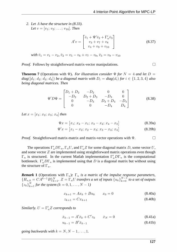
4 Interior-Point Algorithm for MPC-LP
2. LetA have the structure in (8.33).Letv = [v1; v2; . . . ; v10]. Then
A′v =
v1 + Ψ′v2 + Γ′uv3
v3 + v7 + v8v4 + v9 + v10
(8.37)
with v1 = v1 − v2, v2 = v5 − v6 + v7 − v8, v3 = v9 − v10
Proof. Follows by straightforward matrix-vector manipulations.
Theorem 7 (Operations withΨ). For illustration considerΨ for N = 4 and letD =diag([d1; d2; d3; d4]) be a diagonal matrix withDi = diag(di) for i ∈ {1, 2, 3, 4} alsobeing diagonal matrices. Then
Ψ′DΨ =
D1 +D2 −D2 0 0−D2 D2 +D3 −D3 0
0 −D3 D3 +D4 −D4
0 0 −D4 D4
(8.38)
Letx = [x1; x2; x3; x4] then
Ψx =[
x1; x2 − x1; x3 − x2; x4 − x3
]
(8.39a)
Ψ′x =[
x1 − x2; x2 − x3; x3 − x4; x4
]
(8.39b)
Proof. Straightforward matrix-matrix and matrix-vector operations withΨ.
The operationsΓ′uDΓu, ΓuU , andΓ′
uZ for some diagonal matrixD, some vectorU ,and some vectorZ are implemented using straightforward matrix operations even thoughΓu is structured. In the current Matlab implementationΓ′
uDΓu is the computationalbottleneck.Γ′
uDΓu is implemented using thatD is a diagonal matrix but without usingthe structure ofΓu.
Remark 1 (Operations withΓu): Γu is a matrix of the impulse response parameters,{Hu,k = CAk−1B}Nk=1. Z = ΓuU transfers a set of inputs{uk}
N−1k=0 to a set of outputs
{zk}Nk=1 for the system (k = 0, 1, . . . , N − 1)
xk+1 = Axk +Buk x0 = 0 (8.40a)
zk+1 = Cxk+1 (8.40b)
Similarly.U = Γ′uZ corresponds to
xk−1 = A′xk + C ′zk xN = 0 (8.41a)
uk−1 = B′xk−1 (8.41b)
going backwards withk = N,N − 1, . . . , 1.
127
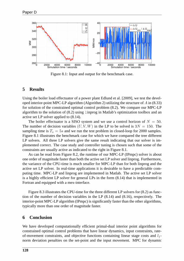
Paper D
Figure 8.1: Input and output for the benchmark case.
5 Results
Using the boiler load effectuator of a power plant Edlund et al. [2009], we test the devel-oped interior-point MPC-LP algorithm (Algorithm 2) utilizing the structure ofA in (8.33)for solution of the constrained optimal control problem (8.2). We compare our MPC-LPalgorithm to the solution of (8.2) usinglinprog in Matlab’s optimization toolbox and anactive set LP solver applied to (8.14).
The boiler effectuator is a SISO system and we use a control horizon ofN = 50.The number of decision variables(U, V,W ) in the LP to be solved is3N = 150. Thesampling time isTs = 5s and we run the test problem in closed-loop for 2000 samples.Figure 8.1 illustrates the benchmark case for which we have compared the tree differentLP solvers. All three LP solvers give the same result indicating that our solver is im-plemented correct. The case study and controller tuning is chosen such that some of theconstraints are usually active as indicated to the right in Figure 8.1.
As can be read from Figure 8.2, the runtime of our MPC-LP (IPmpc) solver is aboutone order of magnitude faster than both the active set LP solver and linprog. Furthermore,the variance of the CPU-time is much smaller for MPC-LP than for both linprog and theactive set LP solver. In real-time applications it is desirable to have a predictable com-puting time. MPC-LP and linprog are implemented in Matlab. The active set LP solveris a highly efficient LP solver for general LPs in the form (8.14) that is implemented inFortran and equipped with a mex-interface.
Figure 8.3 illustrates the CPU-time for the three differentLP solvers for (8.2) as func-tion of the number of decision variables in the LP (8.14) and (8.16), respectively. Theinterior-point MPC-LP algorithm (IPmpc) is significantly faster than the other algorithms,typically more than one order of magnitude faster.
6 Conclusion
We have developed computationally efficient primal-dual interior point algorithms forconstrained optimal control problems that have linear dynamics, input constraints, rate-of-movement constraints, and objective functions containing linear stage costs andl1-norm deviation penalties on the set-point and the input movement. MPC for dynamic
128
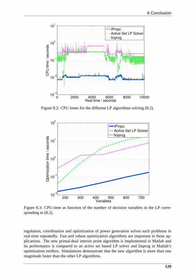
6 Conclusion
Figure 8.2: CPU times for the different LP algorithms solving (8.2).
Figure 8.3: CPU-time as function of the number of decision variables in the LP corre-sponding to (8.2).
regulation, coordination and optimization of power generation solves such problems inreal-time repeatedly. Fast and robust optimization algorithms are important in these ap-plications. The new primal-dual interior point algorithm is implemented in Matlab andits performance is compared to an active set based LP solver and linprog in Matlab’soptimization toolbox. Simulations demonstrate that the new algorithm is more than onemagnitude faster than the other LP algorithms.
129
Paper D
References
J. Allwright and G. Papavasiliou. On Linear Programming andRobust Model-PredictiveControl Using Impulse-Responses.Systems & Control Letters, 18(2):159–164, 1992.
S. Boyd and L. Vandenberghe.Convex Optimization. Cambridge University Press, Cam-bridge, UK, 2004. ISBN 0-521-83378-7.
J. Czyzyk, S. Mehrotra, M. Wagner, and S. J. Wright. PCx: An Interior-Point Code forLinear Programming.Optimization Methods and Software, 11(1):397–430, 1999.
K. Edlund, J. D. Bendtsen, S. Børresen, and T. Mølbak. Introducing Model PredictiveControl for Improving Power Plant Portfolio Performance.Proceedings of the 17thIFAC World Congress, Seoul, South Korea, pages 6986–6991, 2008.
K. Edlund, T. Mølbak, and J. D. Bendtsen. Simple Models for Model-based Portfo-lio Load Balancing Controller Synthesis.Proceedings of IFAC Symposium on powerplants and power systems control 2009, Tampera, Finland, 2009.
J. M. Maciejowski. Predictive Control with Constraints. Pearson Education Limited,2002. ISBN 0-201-39823-0.
S. Mehrotra. On the Implementation of a Primal-Dual Interior Point Method. SIAM J.Optimization, 2(4):575–601, 1992.
A. M. Morshedi, C. R. Cutler, and T. A. Skrovanek. Optimal Solution of Dynamic MatrixControl with Linear Programming Techniques (LDMC). InProceedings of the 1985American Control Conference, Boston, USA, pages 199–208, 1985.
J. Nocedal and S. J. Wright.Numerical Optimization. Springer, New York, 2nd edition,2006. ISBN 0-387-98793-2.
C. V. Rao and J. B. Rawlings. Linear Programming and Model Predictive Control.Jour-nal of Process Control, 10(2–3):283–289, 2000.
C. V. Rao, S. J. Wright, and J. B. Rawlings. Application of Interior-Point Methods toModel Predictive Control.Journal of Optimization Theory and Applications, 99(3):723–757, 1998.
J. B. Rawlings and R. Amrit. Optimizing Process Economic Performance Using ModelPredictive Control. In L. Magni, D. M. Raimondo, and F. Allgower, editors,NonlinearModel Predictive Control, pages 119–138. Springer, 2009. ISBN 3-764-36297-9.
L. Vandenberghe, S. Boyd, and M. Nouralishadi. Robust Linear Programming and Opti-mal Control.Proceedings of 15th IFAC World Congress, Barcelona, Spain, 2002.
S. J. Wright. Primal-Dual Interior-Point Methods. SIAM, Philadelphia, 1997. ISBN0-898-71382-4.
Y. Zhang. Solving Large-Scale Linear Programs by Interior-Point Methods under theMatlab Environment.Optimization Methods and Software, 10(1):1–31, 1998.
130

Paper E
A Dantzig-Wolfe MPC Algorithm for Power Plant Portfolio Cont rol
Kristian Edlund & John Bagterp Jørgensen
This paper was submitted to:International Journal of Control

Copyright c©Taylor & FrancisThe layout has been revised
1 Introduction
Abstract
In this paper we treat the dynamic coordination of a set of constrained, dynam-ically independent systems seeking to achieve one common goal. This is motivatedby a portfolio of multiple power generators which has to follow one production refer-ence for the whole portfolio. A Model Predictive Controller with linear andℓ1-normterms is proposed to coordinate the units. The underlying optimization problem of theproposed controller can be stated as a linear program with a block-angular constraintmatrix. Dantzig-Wolfe decomposition can be successfully applied to decompose thiskind of problems into several subproblems.
Simulations show that the computation time only rises linearly with the numberof units in the problem rather than cubically as is the case when the problem is solvedin a centralized manner with an active-set solver.
1 Introduction
Model Predictive Control (MPC) has successfully been applied in the process industriesfor more than thirty years [Qin and Badgwell, 2003; Lu, 2003;Froisy, 2006]. Sincethe description of the first MPCs based on convolution models[Richalet et al., 1978;Cutler and Ramaker, 1980], several generations of industrial and academic MPCs havelead to the formulation of state space based MPCs [Muske and Rawlings, 1993; Ma-ciejowski, 2002; Rawlings and Mayne, 2009] and in a sense unified the theory of ModelPredictive Control (MPC), Generalized Predictive Control(GPC), and Linear QuadraticGaussian (LQG) regulation [Clarke et al., 1987; Bitmead et al., 1990;Astrom and Wit-tenmark, 1990; Mayne et al., 2000; Jørgensen, 2005]. LinearMPC requires repeatedonline solution of constrained linear or quadratic optimization problems. Therefore, thecomputational speed and robustness of the optimization algorithms has limited the typeof applications that can be controlled by MPC. MPC was originally developed for theprocess industries with relative slow dynamics and a low number of inputs and outputs(say less than 50). As MPC is developed for mechatronic applications with very fast dy-namics, low state order models, and typically less than 3 inputs and outputs, new waysof implementing and solving the constrained optimization problem constituting the MPChave been developed [Bemporad et al., 2002; Diehl et al., 2005; Mattingley and Boyd,2009]. Both process control and mechatronic applications use one centralized MPC tocontrol the system. This is possible because of the low number of inputs and outputs aswell as the relative low number of states in the model.
In this paper we consider a set of dynamically independent systems that must coop-erate to meet a common objective. This is motivated by a portfolio of multiple powergenerators which has to follow one production reference forthe whole portfolio. Themultiple power generator problem is large scale with a very large number of independentsystems. In addition, the system has fast dynamics and must be controlled with a samplerate of approximately 5 seconds. Consequently, such systems cannot be controlled by acentralized approach with one Model Predictive Controllerusing existing optimizationalgorithms due to the large size and fast dynamics. In this paper, we develop a compu-tationally efficient algorithm forℓ1-norm Model Predictive Control of independent lineardynamic systems that must cooperate to meet a common objective. We utilize the specialstructure of the linear program representing the MPC and useDantzig-Wolfe decomposi-
133
Paper E
tion to obtain an efficient optimization algorithm that can solve this class of systems veryfast.
In practice the computational complexity of the optimization problem scales cubicallywith the problem size [Ferris et al., 2007]. Therefore methods to avoid solving the cen-tralized optimization problem must be pursued to successfully apply MPC on large-scalesystems. Lower computationally complexity can be achievedthrough decomposition ofthe control problem, i.e. splitting the problem into multiple smaller problems which areeasier to solve. Much research is going into decomposition of control, an extensive reviewof the area is found in Scattolini [2009].
The strategy followed in this paper is to exploit the structure of the underlying opti-mization problem for decomposition. The decomposition yields a two level hierarchicalcontrol structure. The structure consists of a higher levelsupervisor that coordinatesthe lower level of independent local controllers. The requirement for the method pre-sented in this paper is that the underlying optimization problem is a linear problem witha block-angular constraint structure, i.e. a block diagonal matrix with a set of couplingconstraints involving all variables. The requirement can be achieved by formulating theobjective function withℓ1-norm and linear terms.
A system meeting these requirements can be efficiently decomposed with two meth-ods; Lagrange relaxation [Beasley, 1993] and Dantzig-Wolfe decomposition [Dantzig andWolfe, 1960]. Both methods significantly decrease the computation time for optimizationof linear systems with a block-angular constraint structure. Both methods use an itera-tive scheme to solve the optimization problem. In each iteration the lagrange multipliersattached to the coupling constraints of the problem, are assumed constant. Thereby theoptimization problem is reduced to a block diagonal structure and can be treated asP in-dependent problems. The difference in the two methods is howto find the Lagrange mul-tipliers. Lagrange relaxation computes the multipliers through heuristic methods, whileDantzig-Wolfe decomposition finds the multipliers by solving an optimization problem.Gunnerud et al. [2009] showed that the computation time using Lagrange relaxation isvery sensitive to changes in the problem, and even minor changes might result in a dou-bling of the computation time.
The contribution of this paper is to use Dantzig-Wolfe decomposition for computa-tion of the dynamic calculations of model predictive control and thereby reduce the com-putational complexity compared to the centralized solution without relying on heuristicmethods.
Negenborn et al. [2008] and Rantzer [2009] applied Lagrangerelaxation for decom-posing problems in a model predictive control context. Gunnerud et al. [2009] usedDantzig-Wolfe decomposition for control and planning purposes on a longer time scale,while Cheng et al. [2008] used Dantzig-Wolfe for target calculation in a distributed modelpredictive controller.
There are multiple other approaches to achieve decomposition of controllers. Two ofthem are a decentralized control scheme, meaning that thereis no communication amonglocal controllers [Acar, 1995; Magni and Scattolini, 2006;Raimondo et al., 2007], anddistributed control where local controllers have communication among each other [Jiaand Krogh, 2001; Dunbar, 2007; Zhang and Li, 2007; Venkat et al., 2008]. All of thesepapers treat systems which are dynamically coupled rather than independent. [Keviczkyet al., 2008; Dunbar and Murray, 2006] treats dynamically independent systems that needscoordination to achieve a common goal. The approach in both Keviczky et al. [2008] and
134
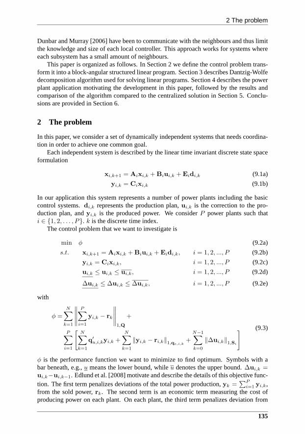
2 The problem
Dunbar and Murray [2006] have been to communicate with the neighbours and thus limitthe knowledge and size of each local controller. This approach works for systems whereeach subsystem has a small amount of neighbours.
This paper is organized as follows. In Section 2 we define the control problem trans-form it into a block-angular structured linear program. Section 3 describes Dantzig-Wolfedecomposition algorithm used for solving linear programs.Section 4 describes the powerplant application motivating the development in this paper, followed by the results andcomparison of the algorithm compared to the centralized solution in Section 5. Conclu-sions are provided in Section 6.
2 The problem
In this paper, we consider a set of dynamically independent systems that needs coordina-tion in order to achieve one common goal.
Each independent system is described by the linear time invariant discrete state spaceformulation
xi,k+1 = Aixi,k + Biui,k + Eidi,k (9.1a)
yi,k = Cixi,k (9.1b)
In our application this system represents a number of power plants including the basiccontrol systems.di,k represents the production plan,ui,k is the correction to the pro-duction plan, andyi,k is the produced power. We considerP power plants such thati ∈ {1, 2, . . . , P}. k is the discrete time index.
The control problem that we want to investigate is
min φ (9.2a)
s.t. xi,k+1 = Aixi,k + Biui,k + Eidi,k, i = 1, 2, ..., P (9.2b)
yi,k = Cixi,k, i = 1, 2, ..., P (9.2c)
ui,k ≤ ui,k ≤ ui,k, i = 1, 2, ..., P (9.2d)
∆ui,k ≤ ∆ui,k ≤ ∆ui,k, i = 1, 2, ..., P (9.2e)
with
φ =N
∑
k=1
∥
∥
∥
∥
∥
P∑
i=1
yi,k − rk
∥
∥
∥
∥
∥
1,Q
+
P∑
i=1
[
N∑
k=1
q′u,i,kyi,k +
N∑
k=1
‖yi,k − ri,k‖1,qe,i,k+
N−1∑
k=0
‖∆ui,k‖1,Si
]
(9.3)
φ is the performance function we want to minimize to find optimum. Symbols with abar beneath, e.g.,u means the lower bound, whileu denotes the upper bound.∆ui,k =ui,k−ui,k−1. Edlund et al. [2008] motivate and describe the details of this objective func-tion. The first term penalizes deviations of the total power production,yk =
∑Pi=1 yi,k,
from the sold power,rk. The second term is an economic term measuring the cost ofproducing power on each plant. On each plant, the third term penalizes deviation from
135
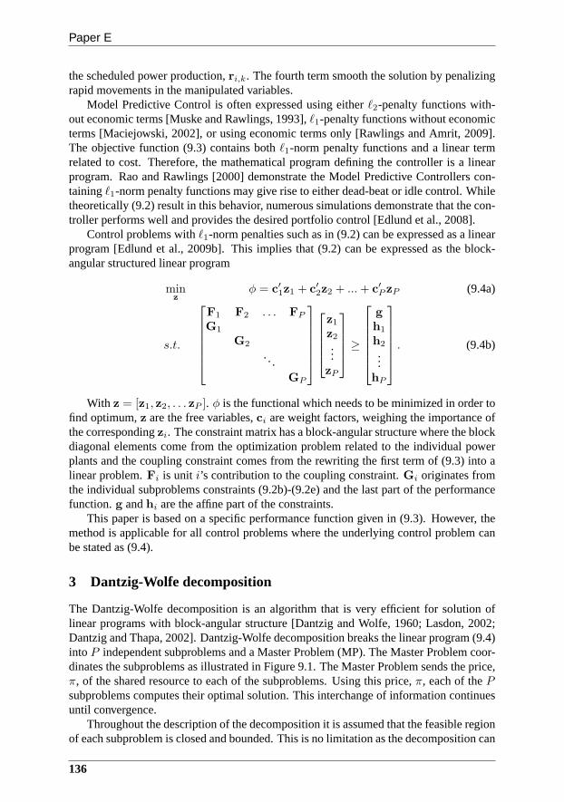
Paper E
the scheduled power production,ri,k. The fourth term smooth the solution by penalizingrapid movements in the manipulated variables.
Model Predictive Control is often expressed using eitherℓ2-penalty functions with-out economic terms [Muske and Rawlings, 1993],ℓ1-penalty functions without economicterms [Maciejowski, 2002], or using economic terms only [Rawlings and Amrit, 2009].The objective function (9.3) contains bothℓ1-norm penalty functions and a linear termrelated to cost. Therefore, the mathematical program defining the controller is a linearprogram. Rao and Rawlings [2000] demonstrate the Model Predictive Controllers con-tainingℓ1-norm penalty functions may give rise to either dead-beat oridle control. Whiletheoretically (9.2) result in this behavior, numerous simulations demonstrate that the con-troller performs well and provides the desired portfolio control [Edlund et al., 2008].
Control problems withℓ1-norm penalties such as in (9.2) can be expressed as a linearprogram [Edlund et al., 2009b]. This implies that (9.2) can be expressed as the block-angular structured linear program
minz
φ = c′1z1 + c′2z2 + ...+ c′P zP (9.4a)
s.t.
F1 F2 . . . FP
G1
G2
. ..GP
z1
z2
...zP
≥
g
h1
h2
...hP
. (9.4b)
With z = [z1, z2, . . . zP ]. φ is the functional which needs to be minimized in order tofind optimum,z are the free variables,ci are weight factors, weighing the importance ofthe correspondingzi. The constraint matrix has a block-angular structure wherethe blockdiagonal elements come from the optimization problem related to the individual powerplants and the coupling constraint comes from the rewritingthe first term of (9.3) into alinear problem.Fi is unit i’s contribution to the coupling constraint.Gi originates fromthe individual subproblems constraints (9.2b)-(9.2e) andthe last part of the performancefunction.g andhi are the affine part of the constraints.
This paper is based on a specific performance function given in (9.3). However, themethod is applicable for all control problems where the underlying control problem canbe stated as (9.4).
3 Dantzig-Wolfe decomposition
The Dantzig-Wolfe decomposition is an algorithm that is very efficient for solution oflinear programs with block-angular structure [Dantzig andWolfe, 1960; Lasdon, 2002;Dantzig and Thapa, 2002]. Dantzig-Wolfe decomposition breaks the linear program (9.4)intoP independent subproblems and a Master Problem (MP). The Master Problem coor-dinates the subproblems as illustrated in Figure 9.1. The Master Problem sends the price,π, of the shared resource to each of the subproblems. Using this price,π, each of thePsubproblems computes their optimal solution. This interchange of information continuesuntil convergence.
Throughout the description of the decomposition it is assumed that the feasible regionof each subproblem is closed and bounded. This is no limitation as the decomposition can
136
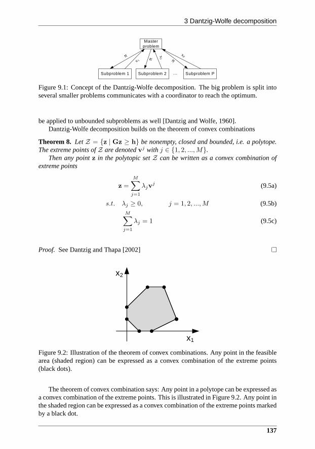
3 Dantzig-Wolfe decomposition
Master problem
Subproblem 1 Subproblem 2 Subproblem P…
π
x 1
x2π π
xP
Figure 9.1: Concept of the Dantzig-Wolfe decomposition. The big problem is split intoseveral smaller problems communicates with a coordinator to reach the optimum.
be applied to unbounded subproblems as well [Dantzig and Wolfe, 1960].Dantzig-Wolfe decomposition builds on the theorem of convex combinations
Theorem 8. LetZ = {z | Gz ≥ h} be nonempty, closed and bounded, i.e. a polytope.The extreme points ofZ are denotedvj with j ∈ {1, 2, ...,M}.
Then any pointz in the polytopic setZ can be written as a convex combination ofextreme points
z =
M∑
j=1
λjvj (9.5a)
s.t. λj ≥ 0, j = 1, 2, ...,M (9.5b)M∑
j=1
λj = 1 (9.5c)
Proof. See Dantzig and Thapa [2002]
x2
x1
Figure 9.2: Illustration of the theorem of convex combinations. Any point in the feasiblearea (shaded region) can be expressed as a convex combination of the extreme points(black dots).
The theorem of convex combination says: Any point in a polytope can be expressed asa convex combination of the extreme points. This is illustrated in Figure 9.2. Any point inthe shaded region can be expressed as a convex combination ofthe extreme points markedby a black dot.
137
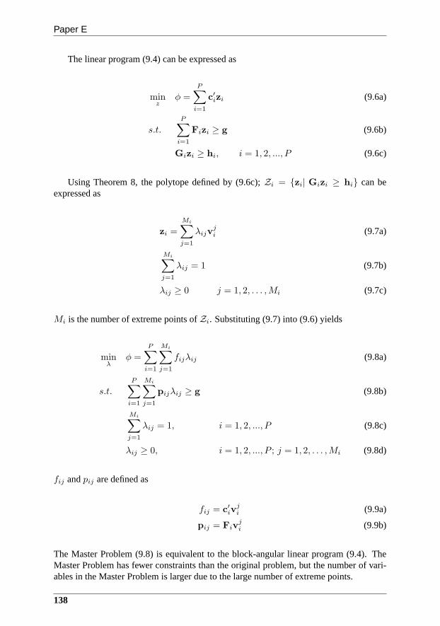
Paper E
The linear program (9.4) can be expressed as
minz
φ =P
∑
i=1
c′izi (9.6a)
s.t.
P∑
i=1
Fizi ≥ g (9.6b)
Gizi ≥ hi, i = 1, 2, ..., P (9.6c)
Using Theorem 8, the polytope defined by (9.6c);Zi = {zi| Gizi ≥ hi} can beexpressed as
zi =
Mi∑
j=1
λijvji (9.7a)
Mi∑
j=1
λij = 1 (9.7b)
λij ≥ 0 j = 1, 2, . . . ,Mi (9.7c)
Mi is the number of extreme points ofZi. Substituting (9.7) into (9.6) yields
minλ
φ =
P∑
i=1
Mi∑
j=1
fijλij (9.8a)
s.t.P
∑
i=1
Mi∑
j=1
pijλij ≥ g (9.8b)
Mi∑
j=1
λij = 1, i = 1, 2, ..., P (9.8c)
λij ≥ 0, i = 1, 2, ..., P ; j = 1, 2, . . . ,Mi (9.8d)
fij andpij are defined as
fij = c′ivji (9.9a)
pij = Fivji (9.9b)
The Master Problem (9.8) is equivalent to the block-angularlinear program (9.4). TheMaster Problem has fewer constraints than the original problem, but the number of vari-ables in the Master Problem is larger due to the large number of extreme points.
138
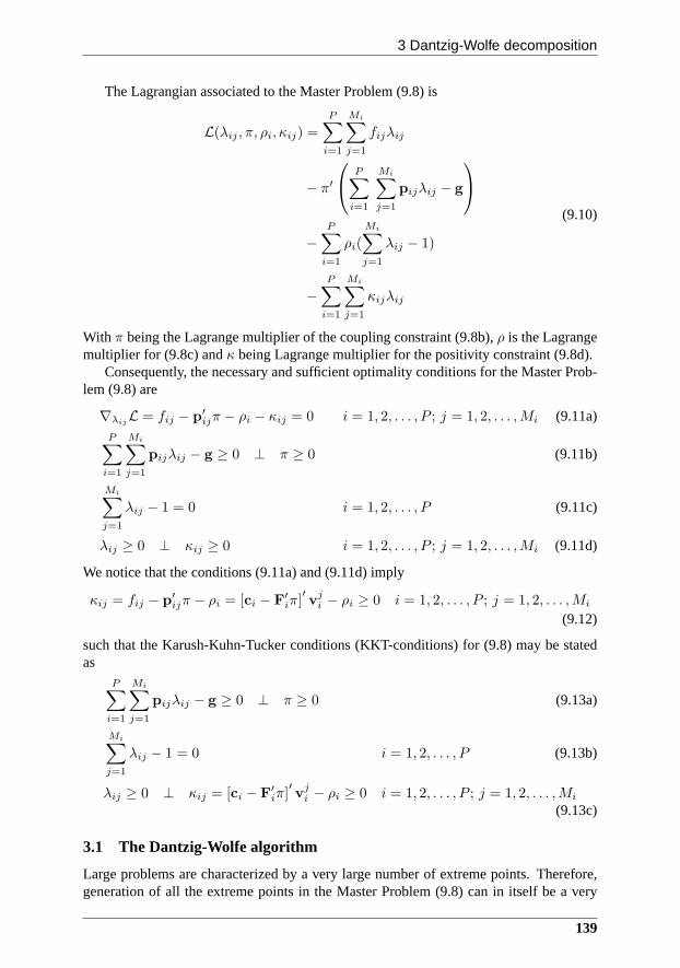
3 Dantzig-Wolfe decomposition
The Lagrangian associated to the Master Problem (9.8) is
L(λij , π, ρi, κij) =
P∑
i=1
Mi∑
j=1
fijλij
− π′
P∑
i=1
Mi∑
j=1
pijλij − g
−P
∑
i=1
ρi(
Mi∑
j=1
λij − 1)
−P
∑
i=1
Mi∑
j=1
κijλij
(9.10)
With π being the Lagrange multiplier of the coupling constraint (9.8b),ρ is the Lagrangemultiplier for (9.8c) andκ being Lagrange multiplier for the positivity constraint (9.8d).
Consequently, the necessary and sufficient optimality conditions for the Master Prob-lem (9.8) are
∇λijL = fij − p′
ijπ − ρi − κij = 0 i = 1, 2, . . . , P ; j = 1, 2, . . . ,Mi (9.11a)P
∑
i=1
Mi∑
j=1
pijλij − g ≥ 0 ⊥ π ≥ 0 (9.11b)
Mi∑
j=1
λij − 1 = 0 i = 1, 2, . . . , P (9.11c)
λij ≥ 0 ⊥ κij ≥ 0 i = 1, 2, . . . , P ; j = 1, 2, . . . ,Mi (9.11d)
We notice that the conditions (9.11a) and (9.11d) imply
κij = fij − p′ijπ − ρi = [ci − F′
iπ]′v
ji − ρi ≥ 0 i = 1, 2, . . . , P ; j = 1, 2, . . . ,Mi
(9.12)
such that the Karush-Kuhn-Tucker conditions (KKT-conditions) for (9.8) may be statedas
P∑
i=1
Mi∑
j=1
pijλij − g ≥ 0 ⊥ π ≥ 0 (9.13a)
Mi∑
j=1
λij − 1 = 0 i = 1, 2, . . . , P (9.13b)
λij ≥ 0 ⊥ κij = [ci − F′iπ]
′v
ji − ρi ≥ 0 i = 1, 2, . . . , P ; j = 1, 2, . . . ,Mi
(9.13c)
3.1 The Dantzig-Wolfe algorithm
Large problems are characterized by a very large number of extreme points. Therefore,generation of all the extreme points in the Master Problem (9.8) can in itself be a very
139
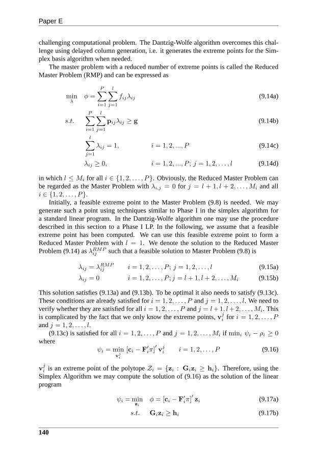
Paper E
challenging computational problem. The Dantzig-Wolfe algorithm overcomes this chal-lenge using delayed column generation, i.e. it generates the extreme points for the Sim-plex basis algorithm when needed.
The master problem with a reduced number of extreme points iscalled the ReducedMaster Problem (RMP) and can be expressed as
minλ
φ =
P∑
i=1
l∑
j=1
fijλij (9.14a)
s.t.
P∑
i=1
l∑
j=1
pijλij ≥ g (9.14b)
l∑
j=1
λij = 1, i = 1, 2, ..., P (9.14c)
λij ≥ 0, i = 1, 2, ..., P ; j = 1, 2, . . . , l (9.14d)
in which l ≤ Mi for all i ∈ {1, 2, . . . , P}. Obviously, the Reduced Master Problem canbe regarded as the Master Problem withλi,j = 0 for j = l + 1, l + 2, . . . ,Mi and alli ∈ {1, 2, . . . , P}.
Initially, a feasible extreme point to the Master Problem (9.8) is needed. We maygenerate such a point using techniques similar to Phase I in the simplex algorithm fora standard linear program. In the Dantzig-Wolfe algorithm one may use the proceduredescribed in this section to a Phase I LP. In the following, weassume that a feasibleextreme point has been computed. We can use this feasible extreme point to form aReduced Master Problem withl = 1. We denote the solution to the Reduced MasterProblem (9.14) asλRMP
ij such that a feasible solution to Master Problem (9.8) is
λij = λRMPij i = 1, 2, . . . , P ; j = 1, 2, . . . , l (9.15a)
λij = 0 i = 1, 2, . . . , P ; j = l + 1, l + 2, . . . ,Mi (9.15b)
This solution satisfies (9.13a) and (9.13b). To be optimal italso needs to satisfy (9.13c).These conditions are already satisfied fori = 1, 2, . . . , P andj = 1, 2, . . . , l. We need toverify whether they are satisfied for alli = 1, 2, . . . , P andj = l+1, l+2, . . . ,Mi. Thisis complicated by the fact that we only know the extreme points,vj
i for i = 1, 2, . . . , Pandj = 1, 2, . . . , l.
(9.13c) is satisfied for alli = 1, 2, . . . , P andj = 1, 2, . . . ,Mi if mini ψi − ρi ≥ 0where
ψi = minv
ji
[ci − F′iπ]
′v
ji i = 1, 2, . . . , P (9.16)
vji is an extreme point of the polytopeZi = {zi : Gizi ≥ hi}. Therefore, using the
Simplex Algorithm we may compute the solution of (9.16) as the solution of the linearprogram
ψi = minzi
φ = [ci − F′iπ]
′zi (9.17a)
s.t. Gizi ≥ hi (9.17b)
140
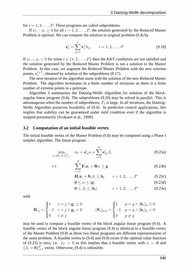
3 Dantzig-Wolfe decomposition
for i = 1, 2, . . . , P . These programs are called subproblems.If ψi − ρi ≥ 0 for all i = 1, 2, . . . , P , the solution generated by the Reduced Master
Problem is optimal. We can compute the solution to original problem (9.4) by
z∗i =l
∑
j=1
vjiλij i = 1, 2, . . . , P (9.18)
If ψi − ρi < 0 for somei ∈ {1, 2, . . . , P} then the KKT conditions are not satisfied andthe solution generated by the Reduced Master Problem is not asolution to the MasterProblem. In this case, we augment the Reduced Master Problemwith the new extremepoints,vl+1
i , obtained by solution of the subproblems (9.17).The next iteration of the algorithm starts with the solutionof the new Reduced Master
Problem. The algorithm terminates in a finite number of iterations as there is a finitenumber of extreme points in a polytope.
Algorithm 3 summarises the Dantzig-Wolfe Algorithm for solution of the block-angular linear program (9.4). The subproblems (9.20) may besolved in parallel. This isadvantageous when the number of subproblems,P , is large. In all iterations, the Dantzig-Wolfe Algorithm preserves feasibility of (9.4). In predictive control applications, thisimplies that stability can be guaranteed under mild condition even if the algorithm isstopped prematurely [Scokaert et al., 1999].
3.2 Computation of an initial feasible vertex
The initial feasible vertex of the Master Problem (9.8) may be computed using a Phase Isimplex algorithm. The linear program
minα,{zi,βi}P
i=1
φI = e′αα+
P∑
i=1
e′βiβi (9.23a)
s.t.P
∑
i=1
Fizi + Rα ≥ g (9.23b)
Hizi + Siβi ≥ hi i = 1, 2, . . . , P (9.23c)
0 ≤ α ≤ |g| (9.23d)
0 ≤ βi ≤ |hi| i = 1, 2, . . . , P (9.23e)
with
Rij =
1 i = j ∧ gi ≥ 0
−1 i = j ∧ gi < 0
0 i 6= j
(Si)p,q =
1 p = q ∧ (hi)p ≥ 0
−1 p = q ∧ (hi)p < 0
0 p 6= q
may be used to compute a feasible vertex of the block angular linear program (9.4). Afeasible vertex of the block angular linear program (9.4) isidentical to a feasible vertexof the Master Problem (9.8) as these two linear programs are different representations ofthe same problem. A feasible vertex to (9.4) and (9.8) existsif the optimal value functionof (9.23) is zero, i.e.φI = 0 as this implies that a feasible vertex withα = 0 and{βi = 0}Pi=1 exists. Otherwise, (9.4) is infeasible.
141
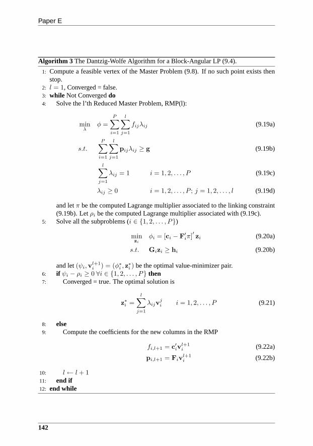
Paper E
Algorithm 3 The Dantzig-Wolfe Algorithm for a Block-Angular LP (9.4).
1: Compute a feasible vertex of the Master Problem (9.8). If no such point exists thenstop.
2: l = 1, Converged = false.3: while Not Convergeddo4: Solve the l’th Reduced Master Problem, RMP(l):
minλ
φ =
P∑
i=1
l∑
j=1
fijλij (9.19a)
s.t.P
∑
i=1
l∑
j=1
pijλij ≥ g (9.19b)
l∑
j=1
λij = 1 i = 1, 2, . . . , P (9.19c)
λij ≥ 0 i = 1, 2, . . . , P ; j = 1, 2, . . . , l (9.19d)
and letπ be the computed Lagrange multiplier associated to the linking constraint(9.19b). Letρi be the computed Lagrange multiplier associated with (9.19c).
5: Solve all the subproblems (i ∈ {1, 2, . . . , P})
minzi
φi = [ci − F′iπ]
′zi (9.20a)
s.t. Gizi ≥ hi (9.20b)
and let(ψi,vl+1i ) = (φ∗i , z
∗i ) be the optimal value-minimizer pair.
6: if ψi − ρi ≥ 0 ∀i ∈ {1, 2, . . . , P} then7: Converged = true. The optimal solution is
z∗i =
l∑
j=1
λijvji i = 1, 2, . . . , P (9.21)
8: else9: Compute the coefficients for the new columns in the RMP
fi,l+1 = c′ivl+1i (9.22a)
pi,l+1 = Fivl+1i (9.22b)
10: l← l + 111: end if12: end while
142
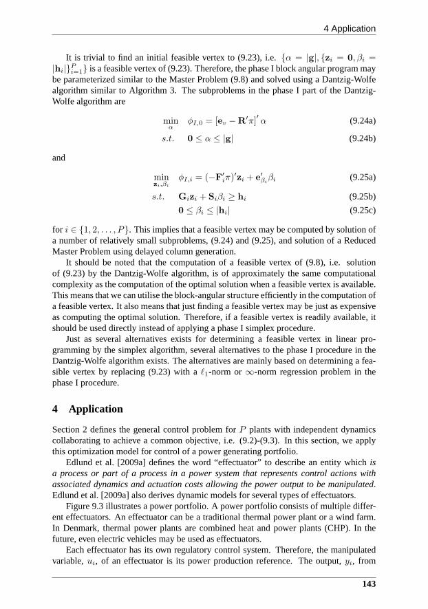
4 Application
It is trivial to find an initial feasible vertex to (9.23), i.e. {α = |g|, {zi = 0, βi =|hi|}
Pi=1} is a feasible vertex of (9.23). Therefore, the phase I block angular program may
be parameterized similar to the Master Problem (9.8) and solved using a Dantzig-Wolfealgorithm similar to Algorithm 3. The subproblems in the phase I part of the Dantzig-Wolfe algorithm are
minα
φI,0 = [ev −R′π]′α (9.24a)
s.t. 0 ≤ α ≤ |g| (9.24b)
and
minzi,βi
φI,i = (−F′iπ)′zi + e′βi
βi (9.25a)
s.t. Gizi + Siβi ≥ hi (9.25b)
0 ≤ βi ≤ |hi| (9.25c)
for i ∈ {1, 2, . . . , P}. This implies that a feasible vertex may be computed by solution ofa number of relatively small subproblems, (9.24) and (9.25), and solution of a ReducedMaster Problem using delayed column generation.
It should be noted that the computation of a feasible vertex of (9.8), i.e. solutionof (9.23) by the Dantzig-Wolfe algorithm, is of approximately the same computationalcomplexity as the computation of the optimal solution when afeasible vertex is available.This means that we can utilise the block-angular structure efficiently in the computation ofa feasible vertex. It also means that just finding a feasible vertex may be just as expensiveas computing the optimal solution. Therefore, if a feasiblevertex is readily available, itshould be used directly instead of applying a phase I simplexprocedure.
Just as several alternatives exists for determining a feasible vertex in linear pro-gramming by the simplex algorithm, several alternatives tothe phase I procedure in theDantzig-Wolfe algorithm exists. The alternatives are mainly based on determining a fea-sible vertex by replacing (9.23) with aℓ1-norm or∞-norm regression problem in thephase I procedure.
4 Application
Section 2 defines the general control problem forP plants with independent dynamicscollaborating to achieve a common objective, i.e. (9.2)-(9.3). In this section, we applythis optimization model for control of a power generating portfolio.
Edlund et al. [2009a] defines the word “effectuator” to describe an entity whichisa process or part of a process in a power system that represents control actions withassociated dynamics and actuation costs allowing the poweroutput to be manipulated.Edlund et al. [2009a] also derives dynamic models for several types of effectuators.
Figure 9.3 illustrates a power portfolio. A power portfolioconsists of multiple differ-ent effectuators. An effectuator can be a traditional thermal power plant or a wind farm.In Denmark, thermal power plants are combined heat and powerplants (CHP). In thefuture, even electric vehicles may be used as effectuators.
Each effectuator has its own regulatory control system. Therefore, the manipulatedvariable,ui, of an effectuator is its power production reference. The output, yi, from
143
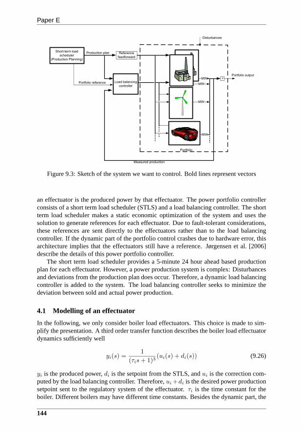
Paper E
Short-term load
scheduler
(Production Planning)
Portfolio
MW
Production plan
Measured production
Load balancing
controller
Reference
feedforward
Disturbances
MW
MW
MW
Portfolio reference
+Portfolio output
Figure 9.3: Sketch of the system we want to control. Bold lines represent vectors
an effectuator is the produced power by that effectuator. The power portfolio controllerconsists of a short term load scheduler (STLS) and a load balancing controller. The shortterm load scheduler makes a static economic optimization ofthe system and uses thesolution to generate references for each effectuator. Due to fault-tolerant considerations,these references are sent directly to the effectuators rather than to the load balancingcontroller. If the dynamic part of the portfolio control crashes due to hardware error, thisarchitecture implies that the effectuators still have a reference. Jørgensen et al. [2006]describe the details of this power portfolio controller.
The short term load scheduler provides a 5-minute 24 hour ahead based productionplan for each effectuator. However, a power production system is complex: Disturbancesand deviations from the production plan does occur. Therefore, a dynamic load balancingcontroller is added to the system. The load balancing controller seeks to minimize thedeviation between sold and actual power production.
4.1 Modelling of an effectuator
In the following, we only consider boiler load effectuators. This choice is made to sim-plify the presentation. A third order transfer function describes the boiler load effectuatordynamics sufficiently well
yi(s) =1
(τis+ 1)3(ui(s) + di(s)) (9.26)
yi is the produced power,di is the setpoint from the STLS, andui is the correction com-puted by the load balancing controller. Therefore,ui +di is the desired power productionsetpoint sent to the regulatory system of the effectuator.τi is the time constant for theboiler. Different boilers may have different time constants. Besides the dynamic part, the
144
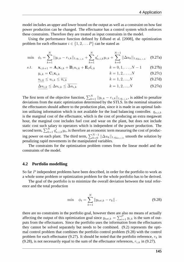
4 Application
model includes an upper and lower bound on the output as well as a constraint on how fastpower production can be changed. The effectuator has a control system which enforcesthese constraints. Therefore they are treated as input constraints in the model.
Using the performance function defined by Edlund et al. [2008], the optimizationproblem for each effectuatori ∈ {1, 2, . . . P} can be stated as
min φi =
N∑
k=1
||yi,k − ri,k||1,qe,i,k+
N∑
k=1
q′u,i,kyi,k +
N−1∑
k=0
||∆uk||1,q∆u,i,k(9.27a)
s.t. xi,k+1 = Aixi,k + Biui,k + Eidi,k k = 0, 1, . . . , N − 1 (9.27b)
yi,k = Cixi,k k = 1, 2, . . . , N (9.27c)
ui,k ≤ ui,k ≤ ui,k k = 1, 2, ..., N (9.27d)
∆ui,k ≤ ∆ui,k ≤ ∆ui,k k = 1, 2, ..., N (9.27e)
The first term of the objective function,∑N
k=1 ||yi,k − ri,k||1,qe,i,k, is added to penalize
deviations from the static optimization determined by the STLS. In the nominal situationthe effectuators should adhere to the production plan, since it is made in an optimal fash-ion utilizing information which is not available for the load balancing controller.qu,i,k
is the marginal cost of the effectuator, which is the cost of producing an extra megawatthour, the marginal cost includes fuel cost and wear on the plant, but does not includestatic cost such salary to operators which is independent ofthe power production. Thesecond term,
∑Nk=1 q
′u,i,kyk, is therefore an economic term measuring the cost of produc-
ing power on each plant. The third term,∑N−1
k=0 ||∆uk||1,q∆u,i,ksmooth the solution by
penalizing rapid movements in the manipulated variables.The constraints for the optimization problem comes from thelinear model and the
constraints of the model.
4.2 Portfolio modelling
So farP independent problems have been described, in order for the portfolio to work asa whole some problem or optimization problem for the whole portfolio has to be derived.
The goal of the portfolio is to minimize the overall deviation between the total refer-ence and the total production
min φt =N
∑
k=1
‖ytot,k − rk‖ . (9.28)
there are no constraints in the portfolio goal, however there are also no means of actuallyaffecting the output of this optimization goal sinceytot,k =
∑Pi=1 yi,k is the sum of out-
puts from the effectuators. Since the portfolio uses the information from the effectuatorsthey cannot be solved separately but needs to be combined. (9.2) represents the opti-mal control problem that combines the portfolio control problem (9.28) with the controlproblem for each effectuator (9.27). It should be noted thatthe portfolio reference,rk in(9.28), is not necessarily equal to the sum of the effectuator references,ri,k in (9.27).
145

Paper E
4.3 Finding an initial feasible solution for the master problem
Rewriting (9.28) into a linear program will add an extra set of decision variables to themaster problem, calledztot. These variables acts similar to slack variables in the sensethat if they are large enough the problem will become feasible. In this case it means thatif a feasible solution can be found to all sub problems, a feasible solution to the MasterProblem exists.
The task of finding an initial feasible solution to the MasterProblem is thereby re-duced to finding a feasible solution to all subproblems withπ = 0. Once a solution toall subproblems are foundztot has to fulfill ztot,k ≥ |
∑Pi=1 yi,k − rk|. Since the right
hand side is known, finding a solution for this inequality is trivial and result in an initialfeasible solution to the Master Problem.
5 Results
Edlund et al. [2008] implement (9.2) as a centralized MPC using a sample time of 5 sec-onds. We also use a sample time of 5 seconds and compare the power portfolio balancingMPC (9.2) implemented using the Dantzig-Wolfe Algorithm described in this paper toa centralized implementation using standard linear programming [Edlund et al., 2008].We investigate the effect of the prediction horizon,N , as well as the effect of the num-ber of effectuators,P , on the computing time for the Dantzig-Wolfe based MPC and thecentralized MPC.
In this section problems of different size will be treated. Each of the Effectuatorshave3N optimization variables and8N constraint equations. The portfolio adds2Nconstraints to the optimization problem. WhereN is the prediction horizon. So withpeffectuators we have a centralized optimization problem with 3Np optimization variablesand8Np + 2N constraints. And when using Dantzig-Wolfe decomposition we havepoptimization problems with3N optimization variables and8N constraints, in addition tothe RMP with2N constraints and a variable number of optimization variables, dependingon the number of iterations needed.
For finding the solution an active-set LP-solver is used which scales cubically withthe number of optimization variables. The solver is used forsolving both the centralizedproblem and the Dantzig-Wolfe decomposition, so the solution times are comparable.
The largest deviation in the elements of the optimal point between the centralizedsolution and the decomposed is of in the magnitude of10−6. That is within the expectedprecision of the algorithm and it is therefore concluded that the two algorithms doesconverge to the same optimal point.
Figure 9.4 shows the average execution time per sample as a function of the numberof effectuators.
The centralized solution scales approximately cubically with the number of effectua-tors. The extra overhead is created from a mixture of the optimizer using more iterationsto converge and MatlabTMcreating more overhead when the problem size grows. TheDantzig-Wolfe decomposition scales almost linearly with the number of effectuators. Partof the overhead in this algorithm comes from the fact that theRMP grows faster whena large number of subsystems are used since a multi column generation scheme is used.The subproblems in the Dantzig-Wolfe decomposition algorithm can be run in parallel.The figure shows a lower bound time estimation for a parallel version of Dantzig-Wolfe
146
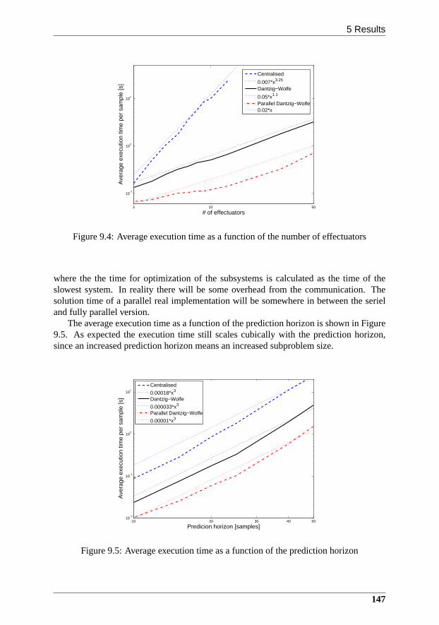
5 Results
103 50
10−1
100
101
# of effectuators
Ave
rage
exe
cutio
n tim
e pe
r sa
mpl
e [s
]
Centralised
0.007*x3.25
Dantzig−Wolfe
0.05*x1.1
Parallel Dantzig−Wolfe0.02*x
Figure 9.4: Average execution time as a function of the number of effectuators
where the the time for optimization of the subsystems is calculated as the time of theslowest system. In reality there will be some overhead from the communication. Thesolution time of a parallel real implementation will be somewhere in between the serieland fully parallel version.
The average execution time as a function of the prediction horizon is shown in Figure9.5. As expected the execution time still scales cubically with the prediction horizon,since an increased prediction horizon means an increased subproblem size.
10 5020 30 4010
−2
10−1
100
101
Predicion horizon [samples]
Ave
rage
exe
cutio
n tim
e pe
r sa
mpl
e [s
]
Centralised
0.00018*x3
Dantzig−Wolfe
0.000033*x3
Parallel Dantzig−Wolfe
0.00001*x3
Figure 9.5: Average execution time as a function of the prediction horizon
147
Paper E
6 Conclusion
We have treated a power portfolio system consisting of multiple dynamically indepen-dent power plants which cooperates to achieve a total production. A Model PredictiveController with linear andℓ1-norm terms has been proposed to coordinate the units. Theunderlying optimization problem of the proposed controller can be stated as a linear pro-gram with a block-angular constraint matrix (9.4). Dantzig-Wolfe decomposition can besuccessfully applied to decompose this kind of problems, yielding a two layer hierarchi-cal optimization structure. The decomposition has a logical physical interpretation as thelower layer consist of independent local controllers for each of the power plants. Theupper level is the supervisor which coordinate the individual units.
The Dantzig-Wolfe decomposition updates and solves the subproblems in an iterativemanner, and will converge to the same optimum as the centralized solution within a finitenumber of iterations. Theoretically the number of iterations may be high, but the sim-ulation results show fast convergence in practical computations. The computation timescales linearly with the number of units in the problem, rather than cubically cubically aswould be the case if the problem is solved in a centralized manner with an interior pointsolver. Dantzig-Wolfe decomposition yields faster solution times than the centralizedsolution even for small number of effectuators.
The proposed Dantzig-Wolfe algorithm scales cubically with the size of the subprob-lems in the as the interior point algorithm, i.e. when the number of constraints or theprediction horizon increases. When the the prediction horizon grows there is algorithmswhich has linear scaling [Rao et al., 1998], this can be exploited when the subproblemsize grows. However,it is not investigated in this paper.
References
L. Acar. Boundaries of the Receding Horizon Control for Interconnected Systems.Jour-nal of Optimization Theory and Applications, 84(2):251–271, 1995.
K. J. Astrom and B. Wittenmark.Computer-controlled Systems. Prentice Hall, 3rd edi-tion, 1990. ISBN 0-133-14899-8.
J. E. Beasley.Modern heuristic techniques for combinatorial problems. John Wiley &Sons, Inc., New York, NY, USA, 1993. ISBN 0-470-22079-1.
A. Bemporad, M. Morari, V. Dua, and E. N. Pistikopoulos. The explicit linear quadraticregulator for constrained systems.Automatica, 38(1):3–20, 2002.
R. R. Bitmead, M. Gevers, and V. Wertz.Adaptive Optimal Control. The Thinking Man’sGPC. Prentice-Hall, New York, NY, USA, 1990. ISBN 0-130-13277-2.
R. Cheng, J. F. Forbes, and W. S. Yip. Dantzig-Wolfe decomposition and plant-wideMPC coordination.Computers and Chemical Engineering, 32(7):1507–1522, 2008.
D. W. Clarke, C. Mohtadi, and P. S. Tuffs. Generalized Predictive Control. Part 1: TheBasic Algorithm.Automatica, 23(2):137–148, 1987.
C. R. Cutler and B. L. Ramaker. Dynamic Matrix Control - A Computer Control Algo-rithm. In Joint American Control Conference, 1980.
148

6 Conclusion
G. B. Dantzig and M. N. Thapa.Linear Programming 2: Theory and Extensions.Springer-Verlag, 2002. ISBN 0-387-98613-8.
G. B. Dantzig and P. Wolfe. Decomposition Principle for Linear Programs.Operationsresearch, 8(1):101–111, 1960.
M. Diehl, H. G. Bock, and J. P. Schloder. A Real-Time Iteration Scheme for NonlinearOptimization in Optimal Feedback Control.SIAM Journal on Control and Optimiza-tion, 43(5):1714–1736, 2005.
W. B. Dunbar. Distributed Receding Horizon Control of Dynamically Coupled NonlinearSystems.IEEE Transactions on Automatic Control, 52(7):1249–1263, 2007.
W. B. Dunbar and R. M. Murray. Distributed Receding horizon control for multi-vehicleformation stabilization.Automatica, 42(4):549–558, 2006.
K. Edlund, J. D. Bendtsen, S. Børresen, and T. Mølbak. Introducing Model PredictiveControl for Improving Power Plant Portfolio Performance.Proceedings of the 17thIFAC World Congress, Seoul, South Korea, pages 6986–6991, 2008.
K. Edlund, T. Mølbak, and J. D. Bendtsen. Simple Models for Model-based Portfo-lio Load Balancing Controller Synthesis.Proceedings of IFAC Symposium on powerplants and power systems control 2009, Tampera, Finland, 2009a.
K. Edlund, L. E. Sokoler, and J. B. Jørgensen. A Primal-Dual Interior-Point Linear Pro-gramming Algorithm for MPC.Proceedings of 48th IEEE Conference on Decision andControl, Shanghai, China, pages 351–356, 2009b.
M. C. Ferris, O. L. Mangasarian, and S. J. Wright.Linear Programming with Matlab.SIAM, 2007. ISBN 0-898-71643-8.
J. B. Froisy. Model predictive control Building a bridge between theory and practice.Computers and Chemical Engineering, 30(10–12):1426–1435, 2006.
V. Gunnerud, B. Foss, B. Nygreen, R. Vestb, and N. C. Walberg.Dantzig-Wolfe decom-position for real-time optimization - applied to the Troll west oil rim. Proceedingsof International Symposium on Advanced Control of ChemicalProcesses, Istanbul,Turkey, 2009.
D. Jia and B. Krogh. Distributed model predictive control.Proceedings of the 2001American Control Conference, Arlington, USA, pages 2767–2772, 2001.
C. Jørgensen, J. H. Mortensen, T. Mølbak, and E. O. Nielsen. Modelbased Fleet Opti-mization and Master Control of a Power Production System. InProceedings of IFACSymposium on Power Plants and Power Systems Control 2006, Kananaskis, Canada,2006.
J. B. Jørgensen.Moving Horizon Estimation and Control. Ph.d. thesis, Technical Univer-sity of Denmark, Kgs. Lyngby, Denmark, 2005.
149
Paper E
T. Keviczky, F. Borelli, K. Fregene, D. Godbole, and G. J. Balas. Decentralised RecedingHorizon Control and Coordination of Autonomous Vehicle Formations. IEEE Trans-actions on Control Systems Technology, 16(1):19–33, 2008.
L. S. Lasdon.Optimization theory for large systems. Dover Publications Inc., 2nd edition,2002. ISBN 0-486-41999-1.
J. Z. Lu. Challenging control problem and emerging technologies in enterprise optimisa-tion. Control Engineering Practice, 11(8):847–858, 2003.
J. M. Maciejowski. Predictive Control with Constraints. Pearson Education Limited,2002. ISBN 0-201-39823-0.
L. Magni and R. Scattolini. Stabilizing decentralized model predictive control of nonlin-ear systems.Automatica, 42(7):1231–1236, 2006.
J. Mattingley and S. Boyd. Automatic Code Generation for Real-Time Convex Optimiza-tion. In Y. Eldar and D. P. Palomar, editors,Convex Optimization in Signal Processingand Communication. Cambridge University Press, Cambridge, UK, 2009.
D. Q. Mayne, J. B. Rawlings, C. V. Rao, and P. O. M. Scokaert. Constrained ModelPredictive Control: Stability and Optimality.Automatica, 36(3):789–814, 2000.
K. R. Muske and J. B. Rawlings. Model Predictive Control withLinear Models.AIChEJournal, 39(2):262–287, 1993.
R. R. Negenborn, B. De. Schutter, and J. Hellendoorn. Multi-agent model predictivecontrol for transportation networks: Serial versus parallel schemes.Engineering Ap-plications of Artificial Intelligence, 21(3):353–366, 2008.
S. J. Qin and T. A. Badgwell. A survey of industrial model predictive control technology.Control Engineering Practice, 11(7):733–764, 2003.
D. M. Raimondo, L. Magni, and R. Scattolini. Decentralized MPC of nonlinear systems:An input-to-state stability approach.International Journal of Robust and NonlinearControl, 17(17):1651–1667, 2007.
A. Rantzer. Dynamic Dual Decomposition for Distributed Control. Proceedings of the2009 conference on American Control Conference, St. Louis,USA, pages 884–888,2009.
C. V. Rao and J. B. Rawlings. Linear Programming and Model Predictive Control.Jour-nal of Process Control, 10(2–3):283–289, 2000.
C. V. Rao, S. J. Wright, and J. B. Rawlings. Application of Interior-Point Methods toModel Predictive Control.Journal of Optimization Theory and Applications, 99(3):723–757, 1998.
J. B. Rawlings and R. Amrit. Optimizing Process Economic Performance Using ModelPredictive Control. In L. Magni, D. M. Raimondo, and F. Allgower, editors,NonlinearModel Predictive Control, pages 119–138. Springer, 2009. ISBN 3-764-36297-9.
150
6 Conclusion
J. B. Rawlings and D. Q. Mayne.Model Predictive Control: Theory and Design. NobHill Publishing, 2009. ISBN 0-975-933770-9.
J. Richalet, A. Rault, J. L. Testud, and J. Papon. Model Predictive Heuristic Control:Applications to Industrial Processes.Automatica, 14(5):413–428, 1978.
R. Scattolini. Architectures for distributed and hierarchical Model Predictive Control.Journal of Process Control, 19(5):723–731, 2009.
P. O. M. Scokaert, D. Q. Mayne, and J. B. Rawlings. SuboptimalModel Predictive control(Feasibility implies Stability).IEEE Transactions on Automatic Control, 44(3):648–654, 1999.
A. N. Venkat, I. A. Hiskens, J. B. Rawlings, and S. J. Wright. Distributed MPC strategieswith application to power system automatic generation control. IEEE Transaction onControl Systems Technology, 16(6):1192–1206, 2008.
Y. Zhang and S. Li. Networked model predictive control basedon neighbourhood opti-mization for serially connected large-scale processes.Journal of Process Control, 17(1):37–50, 2007.
151


Paper F
Hierarchical model-based predictive control of power plant portfolio
Kristian Edlund, Jan Dimon Bendtsen & John Bagterp Jørgensen
This paper was submitted to:Control Engineering Practice

Copyright c©ElsevierThe layout has been revised

1 Introduction
Abstract
This paper describes a design method for developing a flexible hierarchical model-based predictive controller (MPC) for power system portfolio control. The designobjectives are flexibility and computational scalability – since the portfolio will growsignificantly in the future.
The method yields a model predictive controller with a two layer hierarchy andclearly defined interfaces. The same hierarchical structure is achieved on the un-derlying optimization problem utilising Dantzig-Wolfe decomposition. Decompo-sition yields improved computational efficiency and better scalability compared tocentralised methods.
Through simulations on a real scenario the new controller shows improvementsin ability to track reference production and economic performance.
1 Introduction
With the recent (and ongoing) liberalisation of the energy market [Ringel, 2003], in-creasing fuel prices, and increasing political pressure toward the introduction of moresustainable energy into the market [UCTE, 2007; Danish Ministry of Transport and En-ergy, 2005; United Nations, 1998], dynamic control of powerplants is becoming highlyimportant. More than ever, power companies must be able to adapt their production to un-controllable fluctuations in consumer demands as well as in the availability of productionresources, e.g., wind power, at short notice [UCTE, 2007].
Historically, static optimisation of load distribution among power production units,so-calledunit commitment, has been the norm [Padhy, 2004; Salam, 2007]. Unit commit-ment refers to determining the combination of available generating units and schedulingtheir respective outputs to satisfy the forecast demand with the minimum total productioncost under the operating constraints enforced by the systemunder a power company’sjurisdiction (itsportfolio) for a specified period of time – typically from 24 hours up to aweek. The optimisation problem is of high dimension and combinatorial in nature, andcan thus be difficult to solve in practice. Results using Heuristic methods [Johnson et al.,1971; Viana et al., 2001], Mixed Integer Programming [Dillon et al., 1978], DynamicProgramming [Ayuob and Patton, 1971] and Lagrangian Relaxation [Aoki et al., 1987;Shahidehpour and Tong, 1992], have been reported in literature.
Once a solution to the unit comment problem, i.e., a static schedule, has been found,the load plans are distributed to the generating units. Eachunit is then responsible forfollowing its load plan, and must handle disturbances etc. locally, implying the necessityof local power plant controllers, wind farm controllers etc.
However, with the aforementioned increasing impact of short-term fluctuations in thesupply and demand, dynamic effects at the system level will become increasingly incon-venient to deal with for individual generating units. Yet, system-widedynamic portfoliocontrol is a fairly new concept in the field of power production. So far, to the best of theauthors’ knowledge, no results have been reported except Jørgensen et al. [2006]; Edlundet al. [2009a, 2008].
Furthermore, an additional difficulty that will have to be faced in tomorrow’s ‘smartgrids’ is the addition of many more power plants of various types, with different dynamics– e.g., decentralised bio-mass fired thermal units, solar farms and so forth – which meansthat scalability of the control system is set to become an important issue.
155
Paper F
This paper presents a novel, object-oriented design for such a dynamic portfolio con-troller, which is able to handle dynamic disturbances at thesystem level as well as thenon-static configuration of generating units, i.e., the fact that not all units are active atall times. It is based on model-based predictive control (see e.g. Rossiter [2003] and/orRawlings and Mayne [2009] for a comprehensive review) and utilises a decomposed solu-tion scheme tailored specifically to the problem at hand to solve the optimisation problem(see Edlund and Jørgensen [nd] for further details). Tests based on actual operation datafrom the Danish power grid indicate that the proposed controller is able to improve theload following capabilities of the system compared to existing solutions.
The objective of the new controller is to minimise deviations between sold and actualproduction. When designing the controller two objectives have been in focus.
Scalability The future of the power system will require the controller tobe able tocoordinate more units, therefore the method must be scalable in terms of computa-tional complexity.
Flexibility To create a controller which is flexible, such that addition of new unitsand maintenance of existing ones is possible. This means designing a modularstructure with good encapsulation of information and clearcommunication inter-faces between modules.
The outline of the rest of the paper is as follows. In Section 2an overview of the Dan-ish power system is given, including a brief account of the system services the producersmust provide. For comparison purposes, Section 2.3 briefly explains the existing portfo-lio controller. Next, Section 3 presents the proposed control design method and Section4 uses the design method for designing a controller for the current portfolio. Section 5present the comparison of the control performances of the simulations, while Section 6sums up the contributions of this work.
2 System description
To start with the broad perspective, the system is a part of the ENTSO-E, which is theelectrical grid covering the mainland of Europe, from Portugal in the west to Romaniain the east; within this grid, balance between consumption and production must be main-tained at all times. Roughly speaking, if the consumption islarger than the production,energy will be pulled out of the system, making the generators slow down from the usual50Hz and thus a drop in the system frequency can be observed.
In order to maintain the overall balance between productionand consumption ENTSO-E is split into several regions governed by a Transmission System Operator (TSO) whois responsible for matching production with consumption and import/export from the re-gion.
The area treated in this paper is the west Danish area, which is connected synchronouslyto Germany and asynchronously to Norway and Sweden. The major production units areshown in Figure 10.1.
In order to keep balance between production and consumption, a hierarchical schemebased on time horizons is used. Balance between the production and consumption is cur-rently maintained by changing the production, but in some cases consumption might be
156
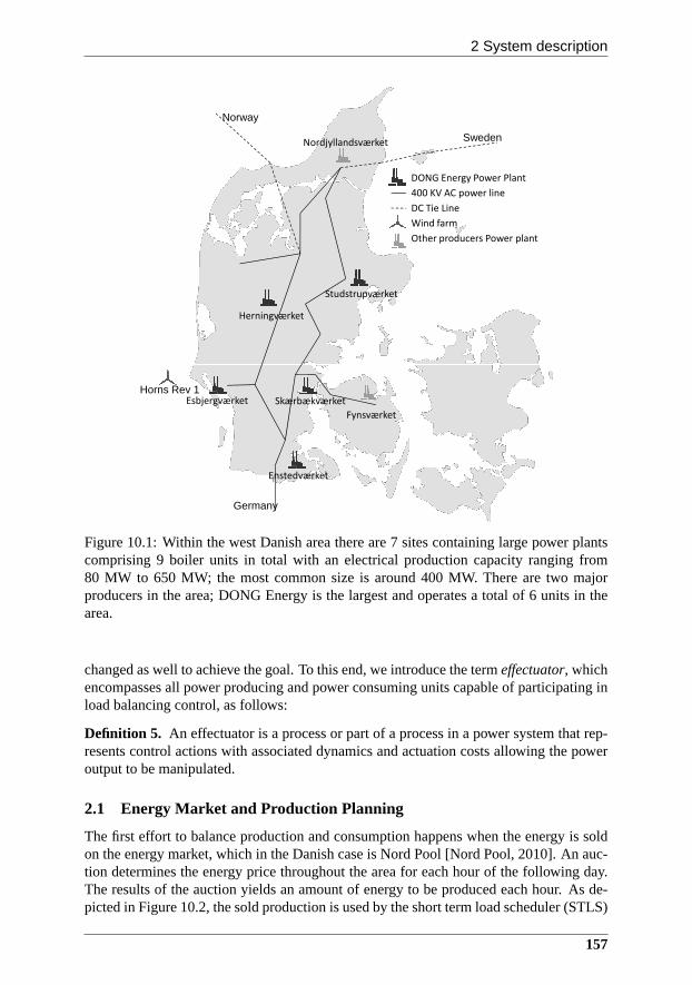
2 System description
Studstrupværket
Herningværket
DONG Energy Power Plant
Horns Rev 1
400 KV AC power line
DC Tie Line
Wind farm
Nordjyllandsværket
Other producers Power plant
Norway
Sweden
Esbjergværket Skærbækværket
Enstedværket
Horns Rev 1
Fynsværket
Germany
Figure 10.1: Within the west Danish area there are 7 sites containing large power plantscomprising 9 boiler units in total with an electrical production capacity ranging from80 MW to 650 MW; the most common size is around 400 MW. There aretwo majorproducers in the area; DONG Energy is the largest and operates a total of 6 units in thearea.
changed as well to achieve the goal. To this end, we introducethe termeffectuator, whichencompasses all power producing and power consuming units capable of participating inload balancing control, as follows:
Definition 5. An effectuator is a process or part of a process in a power system that rep-resents control actions with associated dynamics and actuation costs allowing the poweroutput to be manipulated.
2.1 Energy Market and Production Planning
The first effort to balance production and consumption happens when the energy is soldon the energy market, which in the Danish case is Nord Pool [Nord Pool, 2010]. An auc-tion determines the energy price throughout the area for each hour of the following day.The results of the auction yields an amount of energy to be produced each hour. As de-picted in Figure 10.2, the sold production is used by the short term load scheduler (STLS)
157

Paper F
together with weather forecasts, district heating demand forecasts and constraints such asminimum amount of biomass fuel, to solve a unit commitment problem and compute a5-minute based schedule for all production units in the portfolio that DONG Energy oper-ates, 24 hours ahead. A more detailed description of the STLScan be found in Jørgensenet al. [2006].
TSO
Short-term load
scheduler
(Production Planning)
+
Production plan
Total measured production
Load balancing
controller
+
AGC signal
Filter
Expected
Response
Manual Control
Automatic Control
Measured production of individual units
Sold production
Weather forecast
District heating forecast
+Frequency control
contribution
Reference
Figure 10.2: Diagram of the interconnection of the system. The bold lines show vectorsof signals. The portfolio can be divided into two groups. A manual control which the loadbalancing controller cannot give corrections to, and an automatic control group which theload balancing controller can affect.
2.2 Reserves
Even though the market gives a good estimate of the demand forthe following day, therewill be deviations during the day due to disturbances, inaccurate predictions, weather, etc.Therefore, three levels of control have been established tobalance production and con-sumption. In order to execute the control it is required thata certain production capacityis kept in reserve for that purpose. On the shortest time scale is the primary reserve, whichis used to avoid system collapse. This is then followed up by slower reserves to bring thesystem back to the nominal state. The time scale for activation is shown in Figure 10.3.
When the system frequency deviates from 50 Hz, this reserve isto be activated pro-portional to the system frequency deviation. The reserve has to be activated within 30seconds after a deviation occurs. Details about the reservecan be found in ENTSO-E [2010]. In case of large frequency deviations the primary reserves will be activatedthroughout the whole European grid.
Secondary reserves are used to replace the primary reservesand help restore the sys-tem frequency when they are activated. Each control area, including West Denmark, hassecondary reserves. The control area which hosts an imbalance should seek to activate
158
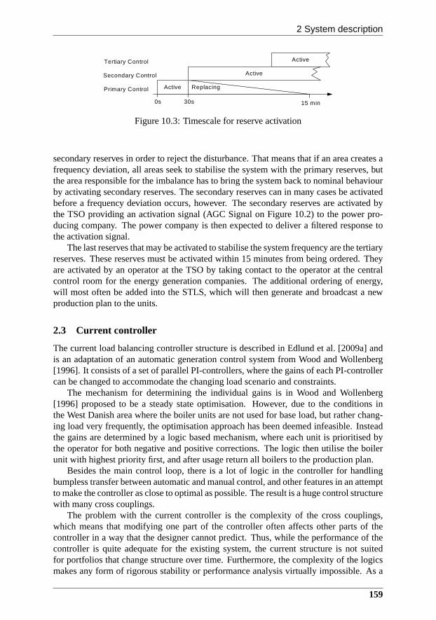
2 System description
30s 15 min
Active
ActiveTertiary Control
Secondary Control
Primary Control
0s
Active
Replacing
Figure 10.3: Timescale for reserve activation
secondary reserves in order to reject the disturbance. Thatmeans that if an area creates afrequency deviation, all areas seek to stabilise the systemwith the primary reserves, butthe area responsible for the imbalance has to bring the system back to nominal behaviourby activating secondary reserves. The secondary reserves can in many cases be activatedbefore a frequency deviation occurs, however. The secondary reserves are activated bythe TSO providing an activation signal (AGC Signal on Figure10.2) to the power pro-ducing company. The power company is then expected to deliver a filtered response tothe activation signal.
The last reserves that may be activated to stabilise the system frequency are the tertiaryreserves. These reserves must be activated within 15 minutes from being ordered. Theyare activated by an operator at the TSO by taking contact to the operator at the centralcontrol room for the energy generation companies. The additional ordering of energy,will most often be added into the STLS, which will then generate and broadcast a newproduction plan to the units.
2.3 Current controller
The current load balancing controller structure is described in Edlund et al. [2009a] andis an adaptation of an automatic generation control system from Wood and Wollenberg[1996]. It consists of a set of parallel PI-controllers, where the gains of each PI-controllercan be changed to accommodate the changing load scenario andconstraints.
The mechanism for determining the individual gains is in Wood and Wollenberg[1996] proposed to be a steady state optimisation. However,due to the conditions inthe West Danish area where the boiler units are not used for base load, but rather chang-ing load very frequently, the optimisation approach has been deemed infeasible. Insteadthe gains are determined by a logic based mechanism, where each unit is prioritised bythe operator for both negative and positive corrections. The logic then utilise the boilerunit with highest priority first, and after usage return all boilers to the production plan.
Besides the main control loop, there is a lot of logic in the controller for handlingbumpless transfer between automatic and manual control, and other features in an attemptto make the controller as close to optimal as possible. The result is a huge control structurewith many cross couplings.
The problem with the current controller is the complexity ofthe cross couplings,which means that modifying one part of the controller often affects other parts of thecontroller in a way that the designer cannot predict. Thus, while the performance of thecontroller is quite adequate for the existing system, the current structure is not suitedfor portfolios that change structure over time. Furthermore, the complexity of the logicsmakes any form of rigorous stability or performance analysis virtually impossible. As a
159
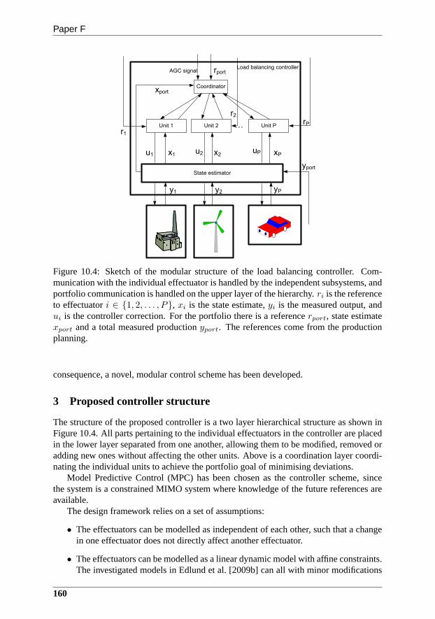
Paper F
Coordinator
Unit P�
Load balancing controller
State estimator
rport
rPUnit 1 Unit 2
r1
AGC signal
xport
y1 y2 yP
u1 u2 uPx1 x2 xP
r2
yport
Figure 10.4: Sketch of the modular structure of the load balancing controller. Com-munication with the individual effectuator is handled by the independent subsystems, andportfolio communication is handled on the upper layer of thehierarchy.ri is the referenceto effectuatori ∈ {1, 2, . . . , P}, xi is the state estimate,yi is the measured output, andui is the controller correction. For the portfolio there is a referencerport, state estimatexport and a total measured productionyport. The references come from the productionplanning.
consequence, a novel, modular control scheme has been developed.
3 Proposed controller structure
The structure of the proposed controller is a two layer hierarchical structure as shown inFigure 10.4. All parts pertaining to the individual effectuators in the controller are placedin the lower layer separated from one another, allowing themto be modified, removed oradding new ones without affecting the other units. Above is acoordination layer coordi-nating the individual units to achieve the portfolio goal ofminimising deviations.
Model Predictive Control (MPC) has been chosen as the controller scheme, sincethe system is a constrained MIMO system where knowledge of the future references areavailable.
The design framework relies on a set of assumptions:
• The effectuators can be modelled as independent of each other, such that a changein one effectuator does not directly affect another effectuator.
• The effectuators can be modelled as a linear dynamic model with affine constraints.The investigated models in Edlund et al. [2009b] can all withminor modifications
160

3 Proposed controller structure
be modelled with the structure shown in Figure 10.5. However, other kinds of linear
Linear process
dynam icsu i y i
M in/m ax Rate lim it M in/m ax
Figure 10.5: General structure of the effectuators
input, output and state constraints fits into the modelling framework as well.
• The underlying optimisation problem in the MPC can be statedas a linear program,which means the corresponding objective function must consist of linear andℓ1-norm terms.
Each object in the lower layer of the hierarchy contains a constrained linear modeland an objective function for the optimal operation of the effectuator which together forma constrained linear programming problem. Furthermore it contains all communicationwith the physical unit. The information that has to be sent tothe upper layer is howthe output of the effectuator will affect the portfolio output, meaning a prediction of thepower production/consumption of the unit.
The upper layer contains a constrained linear model of the portfolio excluding the in-dividually modelled effectuators, as well as an objective function of the optimal operationof the portfolio. The upper layer also handles communication with surrounding systems,for instance obtaining the portfolio reference (the load schedule).
3.1 Solving the optimisation problem
The hierarchical structure encapsulates the information pertaining to each unit. However,one challenge persists: MPC relies on solving an optimisation problem at each sample.This is a challenge of the MPC framework, since solving the optimisation problem usuallygrows cubically with the problem size. Therefore one of the design challenges has beento create an optimisation problem which can be encapsulatedin the same hierarchicalstructure as well as being scalable.
For solving the optimisation problem a Dantzig-Wolfe decomposition approach hasbeen taken [Dantzig and Wolfe, 1960; Dantzig and Thapa, 2002]. The decompositiontechnique has been adapted to the MPC context in Edlund and Jørgensen [nd], wheredetails of the algorithm are also described.
Dantzig-Wolfe decomposition can only be applied to linear problems. The perfor-mance function for the whole problem is assumed to be chosen as a mixture of linear andℓ1-norm terms, which can be rewritten into a linear program suitable for Dantzig-Wolfedecomposition.
An important consequence of this forced choice of performance function and con-straints is the solution, i.e., the point where the performance function attains its extremum,must either be at an extreme point of the feasible set, or the solution of an unconstrainedproblem.
When the optimisation problem is composed from the effectuator optimsation prob-lems and the portfolio optimisation problem it can be rewritten into a linear program withthe structure
161

Paper F
minz
φ = cT1 z1 + cT
2 z2 + ...+ cTP zP (10.1a)
s.t.
F1 F2 . . . FP
G1
G2
. . .GP
z1
z2
...zP
≥
g
h1
h2
...hP
. (10.1b)
with z = [z1, z2, . . . zP ] ∈ Rn, zi ∈ R
ni , φ ∈ R, Fi ∈ Rm×ni , Gi ∈ R
pi×ni , g ∈ Rm
andh ∈ Rpi . φ is the functional which needs to be minimised in order to find optimum,zi
are the free variables,ci are weight factors, weighing the importance of the correspondingzi. The constraint matrix has a block-angular structure wherethe block diagonal elementscome from the effectuator optimisation problem and the coupling constraint comes fromthe portfolio linking the problem together.Fi is unit i’s contribution to the couplingconstraint.Gi originates from the individual effectuators optimisationproblem. g andhi are the affine part of the constraints. Ignoring the couplingconstraints the programconsist ofP independent problems
minzi
φ = cTi zi (10.2a)
s.t. Gizi ≥ hi (10.2b)
Dantzig-Wolfe decomposition builds on the theorem of convex combinations
Theorem 9. LetZ = {z ∈ Rn |Gz ≥ h} with G ∈ R
m×n andh ∈ Rm be nonempty,
closed and bounded, i.e. a polytope. The extreme points ofZ are denotedvj with j ∈{1, 2, ...,M}.
Then any pointz in the polytopic setZ can be written as a convex combination ofextreme points
z =
M∑
j=1
λjvj (10.3a)
s.t. λj ≥ 0, j = 1, 2, ...,M (10.3b)M∑
j=1
λj = 1 (10.3c)
Proof. See [Dantzig and Thapa, 2002]
162

3 Proposed controller structure
Using the theorem on (10.2) and substituting it into (10.1) yields
minλ
φ =
P∑
i=1
Mi∑
j=1
fijλij (10.4a)
s.t.P
∑
i=1
Mi∑
j=1
pijλij ≥ g (10.4b)
Mi∑
j=1
λij = 1, i = 1, 2, ..., P (10.4c)
λij ≥ 0, i = 1, 2, ..., P ; j = 1, 2, . . . ,Mi (10.4d)
With Mi being the number of extreme points of subproblemi. fij andpij are defined as
fij = cTi v
ji (10.5a)
pij = Fivji (10.5b)
Equation (10.4) is denoted the Master Problem. The idea is toonly generate the extremepoints needed for the optimisation instead of generating all extreme points which can beeven more computationally complex due to the size of the problem. Assuming an initialfeasible solution is available for (10.4), a Reduced MasterProblem can be set up andexpanded through iteration with more extreme points. At iteration l the Reduced MasterProblem is defined as
minλ
φ =
P∑
i=1
l∑
j=1
fijλij (10.6a)
s.t.P
∑
i=1
l∑
j=1
pijλij ≥ g (10.6b)
l∑
j=1
λij = 1, i = 1, 2, ..., P (10.6c)
λij ≥ 0, i = 1, 2, ..., P ; j = 1, 2, . . . , l (10.6d)
in which l ≤ Mi for all i ∈ {1, 2, . . . , P}. Obviously, the Reduced Master Problemcan be regarded as the Master Problem withλi,j = 0 for j = l + 1, . . . ,Mi and alli ∈ {1, 2, . . . , P}.
Solving the Reduced Master Problem yields a Lagrange multiplier, π, for the couplingconstraint (10.6b). This can be interpreted as a ’price’ fora shared resource, in this casethe portfolio deviation. New extreme points are generated by solving subproblems definedas
minzi
φ =[
ci − FTi π
]Tzi (10.7a)
s.t. Gizi ≥ hi (10.7b)
163
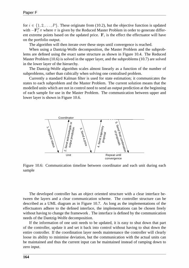
Paper F
for i ∈ {1, 2, . . . , P}. These originate from (10.2), but the objective function isupdatedwith −FT
i π whereπ is given by the Reduced Master Problem in order to generate differ-ent extreme points based on the updated price.Fi is the effect the effectuator will haveon the portfolio output.
The algorithm will then iterate over these steps until convergence is reached.When using a Dantzig-Wolfe decomposition, the Master Problem and the subprob-
lems are defined using the exact same structure as shown in Figure 10.4. The ReducedMaster Problem (10.6) is solved in the upper layer, and the subproblems (10.7) are solvedin the lower layer of the hierarchy.
The Dantzig-Wolfe algorithm scales almost linearly as a function of the number ofsubproblems, rather than cubically when solving one centralised problem.
Currently a standard Kalman filter is used for state estimation; it communicates thestates to each subproblem and the Master Problem. The current solution means that themodelled units which are not in control need to send an outputprediction at the beginningof each sample for use in the Master Problem. The communication between upper andlower layer is shown in Figure 10.6.
Coordinator
Unit
1. Request status
2. S
end
ackn
owle
gde
or
outp
ut p
redi
ctio
n 3. Send a price
4. S
end
traj
ecto
ry
prop
osal
Repeat until convergence
5. Send final com
bination
of proposals
Figure 10.6: Communication timeline between coordinator and each unit during eachsample
The developed controller has an object oriented structure with a clear interface be-tween the layers and a clear communication scheme. The controller structure can bedescribed as a UML diagram as in Figure 10.7. As long as the implementations of theeffectuators adhere to the defined interface, the implementations can be chosen freelywithout having to change the framework . The interface is defined by the communicationneeds of the Dantzig-Wolfe decomposition.
If the information of one unit needs to be updated, it is easy to shut down that partof the controller, update it and set it back into control without having to shut down theentire controller. If the coordination layer needs maintenance the controller will clearlyloose its ability to minimise deviation, but the communication with the actual units canbe maintained and thus the current input can be maintained instead of ramping down tozero input.
164
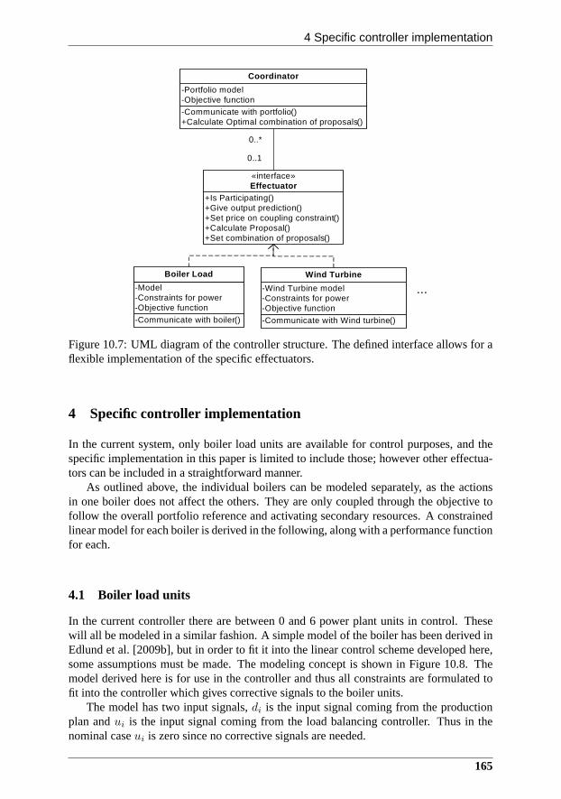
4 Specific controller implementation
-Communicate with portfolio()+Calculate Optimal combination of proposals()
-Portfolio model-Objective function
Coordinator
+Is Participating()+Give output prediction()+Set price on coupling constraint()+Calculate Proposal()+Set combination of proposals()
«interface»Effectuator
-Communicate with boiler()
-Model-Constraints for power-Objective function
Boiler Load
-Communicate with Wind turbine()
-Wind Turbine model-Constraints for power-Objective function
Wind Turbine
...
0..*
0..1
Figure 10.7: UML diagram of the controller structure. The defined interface allows for aflexible implementation of the specific effectuators.
4 Specific controller implementation
In the current system, only boiler load units are available for control purposes, and thespecific implementation in this paper is limited to include those; however other effectua-tors can be included in a straightforward manner.
As outlined above, the individual boilers can be modeled separately, as the actionsin one boiler does not affect the others. They are only coupled through the objective tofollow the overall portfolio reference and activating secondary resources. A constrainedlinear model for each boiler is derived in the following, along with a performance functionfor each.
4.1 Boiler load units
In the current controller there are between 0 and 6 power plant units in control. Thesewill all be modeled in a similar fashion. A simple model of theboiler has been derived inEdlund et al. [2009b], but in order to fit it into the linear control scheme developed here,some assumptions must be made. The modeling concept is shownin Figure 10.8. Themodel derived here is for use in the controller and thus all constraints are formulated tofit into the controller which gives corrective signals to theboiler units.
The model has two input signals,di is the input signal coming from the productionplan andui is the input signal coming from the load balancing controller. Thus in thenominal caseui is zero since no corrective signals are needed.
165
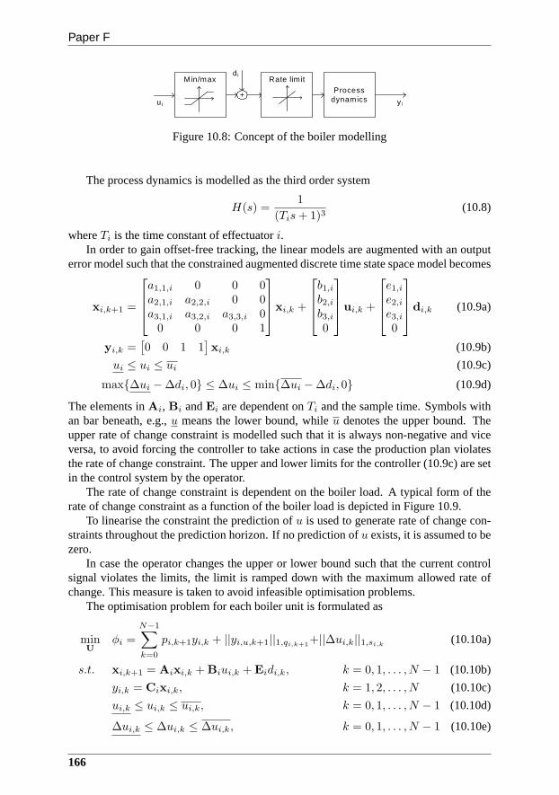
Paper F
u i y i
Process dynamics
Min/max Rate lim it
+
d i
Figure 10.8: Concept of the boiler modelling
The process dynamics is modelled as the third order system
H(s) =1
(Tis+ 1)3(10.8)
whereTi is the time constant of effectuatori.In order to gain offset-free tracking, the linear models areaugmented with an output
error model such that the constrained augmented discrete time state space model becomes
xi,k+1 =
a1,1,i 0 0 0a2,1,i a2,2,i 0 0a3,1,i a3,2,i a3,3,i 0
0 0 0 1
xi,k +
b1,i
b2,i
b3,i
0
ui,k +
e1,i
e2,i
e3,i
0
di,k (10.9a)
yi,k =[
0 0 1 1]
xi,k (10.9b)
ui ≤ ui ≤ ui (10.9c)
max{∆ui −∆di, 0} ≤ ∆ui ≤ min{∆ui −∆di, 0} (10.9d)
The elements inAi, Bi andEi are dependent onTi and the sample time. Symbols withan bar beneath, e.g.,u means the lower bound, whileu denotes the upper bound. Theupper rate of change constraint is modelled such that it is always non-negative and viceversa, to avoid forcing the controller to take actions in case the production plan violatesthe rate of change constraint. The upper and lower limits forthe controller (10.9c) are setin the control system by the operator.
The rate of change constraint is dependent on the boiler load. A typical form of therate of change constraint as a function of the boiler load is depicted in Figure 10.9.
To linearise the constraint the prediction ofu is used to generate rate of change con-straints throughout the prediction horizon. If no prediction ofu exists, it is assumed to bezero.
In case the operator changes the upper or lower bound such that the current controlsignal violates the limits, the limit is ramped down with themaximum allowed rate ofchange. This measure is taken to avoid infeasible optimisation problems.
The optimisation problem for each boiler unit is formulatedas
minU
φi =
N−1∑
k=0
pi,k+1yi,k + ||yi,u,k+1||1,qi,k+1+||∆ui,k||1,si,k
(10.10a)
s.t. xi,k+1 = Aixi,k + Biui,k + Eidi,k, k = 0, 1, . . . , N − 1 (10.10b)
yi,k = Cixi,k, k = 1, 2, . . . , N (10.10c)
ui,k ≤ ui,k ≤ ui,k, k = 0, 1, . . . , N − 1 (10.10d)
∆ui,k ≤ ∆ui,k ≤ ∆ui,k, k = 0, 1, . . . , N − 1 (10.10e)
166

4 Specific controller implementation
Rate of Change [MW/Min]
u [%]
0% 100%mediumlow high
Figure 10.9: Actual rate of change constraint as a function of boiler load. This statedependency is not captured in the constraint (10.9d), but a linearisation based on theprediction is used in the model.
whereUi = [ui,0, ui,1, ..., ui,N−1]T , andAi,Bi,Ci,Ei given in (10.9a) and (10.9b).
The first term in the performance functionpi,k−1yi,k is a linear term representing thecost of the boiler unit. The weightpi,k+1 is the marginal cost, i.e., the cost for producingenergy on the boiler unit. The price is calculated based on the fuel prices and boilerefficiency. The efficiency is state-dependent. For the calculations ofpi,k+1, it is based onthe production plan alone.
It is assumed that the production plan from the STLS is optimal, and thus in thenominal case the correction signal from the load balancing controller should be zero. Inorder to avoid that the load balancing controller maximisesthe production of the cheapestunits, and minimise the production of the most expensive units the term||yu,k−1||1,qy,k−1
is added. This term penalises the part of the output coming from the controller corrections.The last term of the performance function is a penalty on rapid changes on the correc-
tion signal.This optimisation problem is the controller for uniti, and this information is stored in
each of the effectuators on the lower layer of the hierarchy.
Primary reserve handling
Figure 10.10 shows an example of the maximum reserve available in both up and downdirection as a function of the unit load. Reserves availablefor the positive and negativecorrections are shown in the right and left half planes respectively.
Currently the Frequency Control Scheduler makes reservations of the reserves peri-odically. That means it might reserve 5MW of positive correction and 10MW of negativecorrection power from a specific unit at a given time.
It is chosen to give first priority to the Frequency Control Scheduler, and let it makethe reservations. Once the reservations are known, the upper and lower bound for theunit can be determined, such that the reserved primary reserve can be delivered. Theseupper and lower bounds are enforced on the load balancing controller along with upperand lower bounds set by the operator.
167
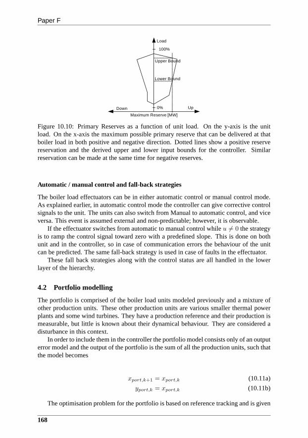
Paper F
Load
Maximum Reserve [MW]
0%
100%
UpDown
Lower Bound
Upper Bound
Figure 10.10: Primary Reserves as a function of unit load. Onthe y-axis is the unitload. On the x-axis the maximum possible primary reserve that can be delivered at thatboiler load in both positive and negative direction. Dottedlines show a positive reservereservation and the derived upper and lower input bounds forthe controller. Similarreservation can be made at the same time for negative reserves.
Automatic / manual control and fall-back strategies
The boiler load effectuators can be in either automatic control or manual control mode.As explained earlier, in automatic control mode the controller can give corrective controlsignals to the unit. The units can also switch from Manual to automatic control, and viceversa. This event is assumed external and non-predictable;however, it is observable.
If the effectuator switches from automatic to manual control while u 6= 0 the strategyis to ramp the control signal toward zero with a predefined slope. This is done on bothunit and in the controller, so in case of communication errors the behaviour of the unitcan be predicted. The same fall-back strategy is used in caseof faults in the effectuator.
These fall back strategies along with the control status areall handled in the lowerlayer of the hierarchy.
4.2 Portfolio modelling
The portfolio is comprised of the boiler load units modeled previously and a mixture ofother production units. These other production units are various smaller thermal powerplants and some wind turbines. They have a production reference and their production ismeasurable, but little is known about their dynamical behaviour. They are considered adisturbance in this context.
In order to include them in the controller the portfolio model consists only of an outputerror model and the output of the portfolio is the sum of all the production units, such thatthe model becomes
xport,k+1 = xport,k (10.11a)
yport,k = xport,k (10.11b)
The optimisation problem for the portfolio is based on reference tracking and is given
168
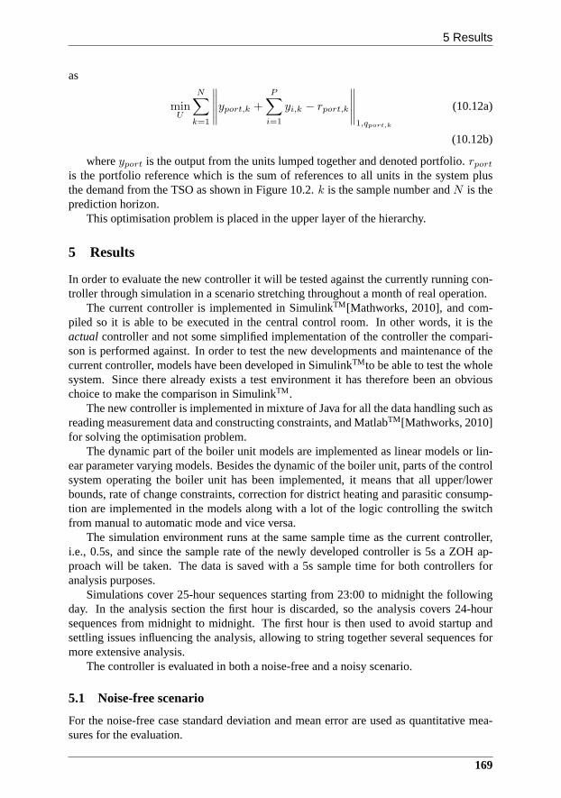
5 Results
as
minU
N∑
k=1
∥
∥
∥
∥
∥
yport,k +
P∑
i=1
yi,k − rport,k
∥
∥
∥
∥
∥
1,qport,k
(10.12a)
(10.12b)
whereyport is the output from the units lumped together and denoted portfolio. rport
is the portfolio reference which is the sum of references to all units in the system plusthe demand from the TSO as shown in Figure 10.2.k is the sample number andN is theprediction horizon.
This optimisation problem is placed in the upper layer of thehierarchy.
5 Results
In order to evaluate the new controller it will be tested against the currently running con-troller through simulation in a scenario stretching throughout a month of real operation.
The current controller is implemented in SimulinkTM [Mathworks, 2010], and com-piled so it is able to be executed in the central control room.In other words, it is theactualcontroller and not some simplified implementation of the controller the compari-son is performed against. In order to test the new developments and maintenance of thecurrent controller, models have been developed in SimulinkTM to be able to test the wholesystem. Since there already exists a test environment it hastherefore been an obviouschoice to make the comparison in SimulinkTM .
The new controller is implemented in mixture of Java for all the data handling such asreading measurement data and constructing constraints, and MatlabTM [Mathworks, 2010]for solving the optimisation problem.
The dynamic part of the boiler unit models are implemented aslinear models or lin-ear parameter varying models. Besides the dynamic of the boiler unit, parts of the controlsystem operating the boiler unit has been implemented, it means that all upper/lowerbounds, rate of change constraints, correction for district heating and parasitic consump-tion are implemented in the models along with a lot of the logic controlling the switchfrom manual to automatic mode and vice versa.
The simulation environment runs at the same sample time as the current controller,i.e., 0.5s, and since the sample rate of the newly developed controller is 5s a ZOH ap-proach will be taken. The data is saved with a 5s sample time for both controllers foranalysis purposes.
Simulations cover 25-hour sequences starting from 23:00 tomidnight the followingday. In the analysis section the first hour is discarded, so the analysis covers 24-hoursequences from midnight to midnight. The first hour is then used to avoid startup andsettling issues influencing the analysis, allowing to string together several sequences formore extensive analysis.
The controller is evaluated in both a noise-free and a noisy scenario.
5.1 Noise-free scenario
For the noise-free case standard deviation and mean error are used as quantitative mea-sures for the evaluation.
169
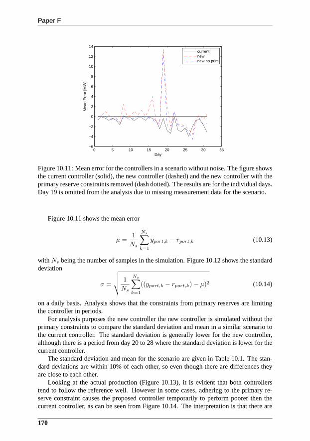
Paper F
0 5 10 15 20 25 30 35−6
−4
−2
0
2
4
6
8
10
12
14
Day
Mea
n E
rror
[MW
]
currentnewnew no prim
Figure 10.11: Mean error for the controllers in a scenario without noise. The figure showsthe current controller (solid), the new controller (dashed) and the new controller with theprimary reserve constraints removed (dash dotted). The results are for the individual days.Day 19 is omitted from the analysis due to missing measurement data for the scenario.
Figure 10.11 shows the mean error
µ =1
Ns
Ns∑
k=1
yport,k − rport,k (10.13)
with Ns being the number of samples in the simulation. Figure 10.12 shows the standarddeviation
σ =
√
√
√
√
1
Ns
Ns∑
k=1
((yport,k − rport,k)− µ)2 (10.14)
on a daily basis. Analysis shows that the constraints from primary reserves are limitingthe controller in periods.
For analysis purposes the new controller the new controlleris simulated without theprimary constraints to compare the standard deviation and mean in a similar scenario tothe current controller. The standard deviation is generally lower for the new controller,although there is a period from day 20 to 28 where the standarddeviation is lower for thecurrent controller.
The standard deviation and mean for the scenario are given inTable 10.1. The stan-dard deviations are within 10% of each other, so even though there are differences theyare close to each other.
Looking at the actual production (Figure 10.13), it is evident that both controllerstend to follow the reference well. However in some cases, adhering to the primary re-serve constraint causes the proposed controller temporarily to perform poorer then thecurrent controller, as can be seen from Figure 10.14. The interpretation is that there are
170
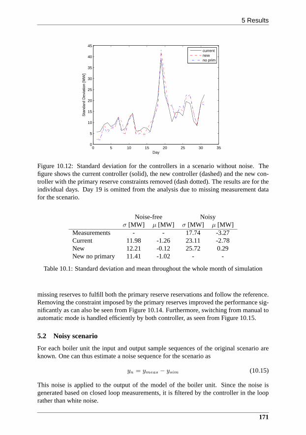
5 Results
0 5 10 15 20 25 30 350
5
10
15
20
25
30
35
40
45
Day
Sta
ndar
d D
evia
tion
[MW
]
currentnewno prim
Figure 10.12: Standard deviation for the controllers in a scenario without noise. Thefigure shows the current controller (solid), the new controller (dashed) and the new con-troller with the primary reserve constraints removed (dashdotted). The results are for theindividual days. Day 19 is omitted from the analysis due to missing measurement datafor the scenario.
Noise-free Noisyσ [MW] µ [MW] σ [MW] µ [MW]
Measurements - - 17.74 -3.27Current 11.98 -1.26 23.11 -2.78New 12.21 -0.12 25.72 0.29New no primary 11.41 -1.02 - -
Table 10.1: Standard deviation and mean throughout the whole month of simulation
missing reserves to fulfill both the primary reserve reservations and follow the reference.Removing the constraint imposed by the primary reserves improved the performance sig-nificantly as can also be seen from Figure 10.14. Furthermore, switching from manual toautomatic mode is handled efficiently by both controller, asseen from Figure 10.15.
5.2 Noisy scenario
For each boiler unit the input and output sample sequences ofthe original scenario areknown. One can thus estimate a noise sequence for the scenario as
yn = ymeas − ysim (10.15)
This noise is applied to the output of the model of the boiler unit. Since the noise isgenerated based on closed loop measurements, it is filtered by the controller in the looprather than white noise.
171

Paper F
0 500 1000 1500400
500
600
700
800
900
1000
1100
1200
1300
Time [minutes]
Pro
duct
ion
[MW
]
ReferenceCurrentNewNew no prim
Figure 10.13: The production of day 3 in the scenario. Both controllers tend to follow thereference well. Both the new controller (dotted line) and the current controller (dashedline), follow the reference (solid line) well.
340 350 360 370 380 390 400 410 420 430 440
450
500
550
600
650
700
750
Time [minutes]
Pro
duct
ion
[MW
]
ReferenceCurrentNewNew no prim
Figure 10.14: Section of the production on day 3, showing a period where the primaryconstraint is active and thus limits the new controller (dotted line) from reaching thereference (solid line). Removing this constraint make the new controller (dash dottedline) perform similar to the current controller (dashed line).
172

5 Results
580 600 620 640 660 680800
850
900
950
1000
1050
1100
1150
1200
1250
1300
Time [minutes]
Pro
duct
ion
[MW
]
ReferenceCurrentNewNew no prim
Unit switched to automatic control
Figure 10.15: Section of day, where a power plant is switchedfrom manual to automaticcontrol. Both the new controller (dotted line) and the current controller (dashed line)handle this event in a bumpless fashion and follow the reference (solid line) well.
This noise generation is chosen in order for the simulation scenario to resemble theactual scenario as closely as possible including failures.The measurements from the unitsmodelled as the portfolio are applied directly to the simulation without filtering.
The mean and standard deviation are once again used as quantitative measures forcontroller performance. The price difference between the controllers can be calculatedgiven fuel costs and deviation prices.
The standard deviation on the new controller is higher than the current controller aswas the case in the noise-free scenario. Both are significantly higher than the measure-ment data which is likely caused by the noise generation scheme as shown in Figure 10.17.The trend in standard deviation is the same for both controllers and measurement data.As seen in the noise-free scenario, the current controller has a slightly better performancethan the proposed.
The mean error is larger in the noisy scenario compared to thenoise-free. Though notconsistently lower, the average shown in Table 10.1 shows that the new controller is anorder of magnitude closer to zero mean error compared to the current controller.
Figure 10.18 shows the price difference between the two controllers. Analysing theprice shows that on most days the new controller performs better in terms of income. OnDay 20 the primary reserves limits the controller such that alarge deviation occurs overa long period of time, which is detrimental for the earnings of the controller. On averagethe difference is 240e/day, which means an earning of almost 90.000e/year.
5.3 Execution time
The benefits of using Dantzig-Wolfe decomposition, besidesthe very logical decomposi-tion, is that the execution time scales almost linearly withthe number of units in controland that the problem can be easily distributed amongst multiple processors and thus low-
173

Paper F
0 5 10 15 20 25 30 35−20
−15
−10
−5
0
5
10
15
20
Day
Mea
n E
rror
[MW
]
MeasurementsCurrentNew
Figure 10.16: Mean error for the controllers in a noisy scenario. The figure shows thecurrent controller (solid), the new controller (dashed) and the new controller with theprimary reserve constraints removed (dash dotted). The results are for the individual days.Day 19 is omitted from the analysis due to missing measurement data for the scenario.
ering the execution time further.As a benchmark of execution time, day 24 is chosen, where 4 units are controlled.
Prediction horizon [samples] Execution time [s]5 69115 124525 360235 12960
Table 10.2: Execution time as a function prediction horizon
Table 10.2 shows the execution time as a function of the prediction horizon. Thesesimulations are performed on a Dual Core Intel Xeon machine running at 2.53GHz with4GB RAM and using Windows Vista as operating system. A 25 hours simulation can beperformed in just about an hour. This timing is including thesimulation.
Increasing the prediction horizon significantly increase the execution time of the con-troller. This has two explanations, one is the obvious that the problem size grows, andit was shown in Edlund and Jørgensen [nd] that the execution time grows cubically withthe prediction horizon. Secondly the algorithm may benefit from better handling of fastvs. slow unit dynamics (compared to the prediction horizon). This is subject of futureresearch.
174
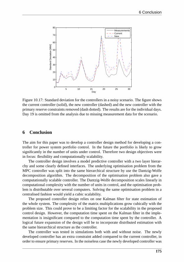
6 Conclusion
5 10 15 20 25 300
10
20
30
40
50
60
70
80
Day
Sta
ndar
d D
evia
tion
[MW
]
MeasurementsCurrentNew
Figure 10.17: Standard deviation for the controllers in a noisy scenario. The figure showsthe current controller (solid), the new controller (dashed) and the new controller with theprimary reserve constraints removed (dash dotted). The results are for the individual days.Day 19 is omitted from the analysis due to missing measurement data for the scenario.
6 Conclusion
The aim for this paper was to develop a controller design method for developing a con-troller for power system portfolio control. In the future the portfolio is likely to growsignificantly in the number of units under control. Therefore two design objectives werein focus: flexibility and computationally scalability.
The controller design involves a model predictive controller with a two layer hierar-chy and some clearly defined interfaces. The underlying optimisation problem from theMPC controller was split into the same hierarchical structure by use the Dantzig-Wolfedecomposition algorithm. The decomposition of the optimisation problem also gave acomputationally scalable controller. The Dantzig-Wolfe decomposition scales linearly incomputational complexity with the number of units in control, and the optimisation prob-lem is distributable over several computers. Solving the same optimisation problem in acentralised fashion would yield a cubic scalability.
The proposed controller design relies on one Kalman filter for state estimation ofthe whole system. The complexity of the matrix multiplications grow cubically with theproblem size. This could prove to be a limiting factor for thescalability in the proposedcontrol design. However, the computation time spent on the Kalman filter in the imple-mentation is insignificant compared to the computation timespent by the controller. Alogical future expansion of the design will be to incorporate distributed estimation withthe same hierarchical structure as the controller.
The controller was tested in simulations both with and without noise. The newlydeveloped controller has an extra constraint added compared to the current controller, inorder to ensure primary reserves. In the noiseless case the newly developed controller was
175
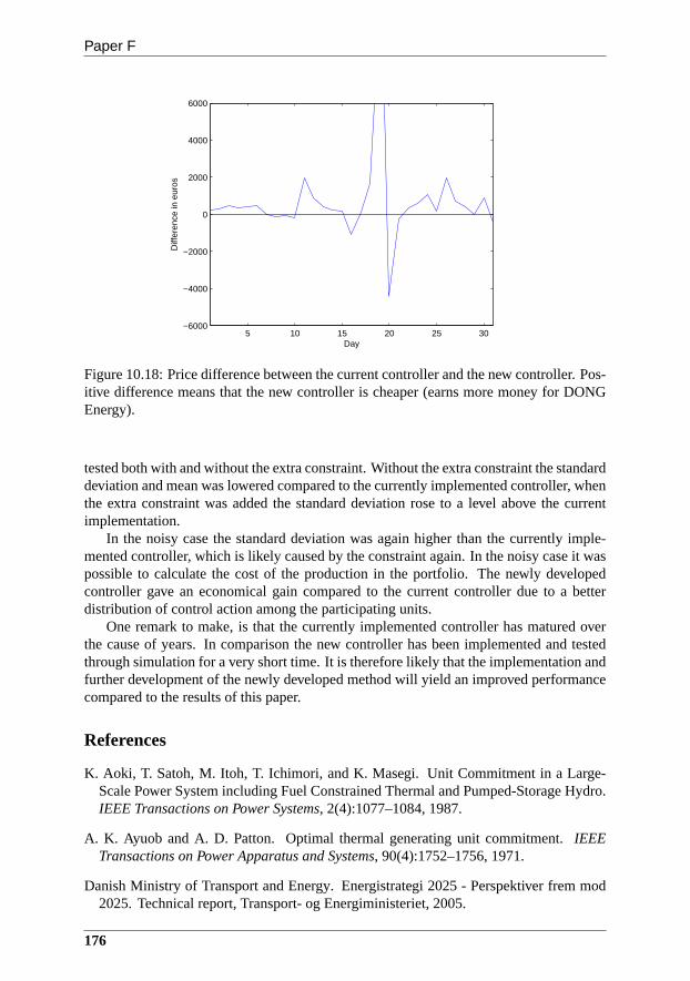
Paper F
5 10 15 20 25 30−6000
−4000
−2000
0
2000
4000
6000
Day
Diff
eren
ce in
eur
os
Figure 10.18: Price difference between the current controller and the new controller. Pos-itive difference means that the new controller is cheaper (earns more money for DONGEnergy).
tested both with and without the extra constraint. Without the extra constraint the standarddeviation and mean was lowered compared to the currently implemented controller, whenthe extra constraint was added the standard deviation rose to a level above the currentimplementation.
In the noisy case the standard deviation was again higher than the currently imple-mented controller, which is likely caused by the constraintagain. In the noisy case it waspossible to calculate the cost of the production in the portfolio. The newly developedcontroller gave an economical gain compared to the current controller due to a betterdistribution of control action among the participating units.
One remark to make, is that the currently implemented controller has matured overthe cause of years. In comparison the new controller has beenimplemented and testedthrough simulation for a very short time. It is therefore likely that the implementation andfurther development of the newly developed method will yield an improved performancecompared to the results of this paper.
References
K. Aoki, T. Satoh, M. Itoh, T. Ichimori, and K. Masegi. Unit Commitment in a Large-Scale Power System including Fuel Constrained Thermal and Pumped-Storage Hydro.IEEE Transactions on Power Systems, 2(4):1077–1084, 1987.
A. K. Ayuob and A. D. Patton. Optimal thermal generating unitcommitment. IEEETransactions on Power Apparatus and Systems, 90(4):1752–1756, 1971.
Danish Ministry of Transport and Energy. Energistrategi 2025 - Perspektiver frem mod2025. Technical report, Transport- og Energiministeriet,2005.
176

6 Conclusion
G. B. Dantzig and M. N. Thapa.Linear Programming 2: Theory and Extensions.Springer-Verlag, 2002. ISBN 0-387-98613-8.
G. B. Dantzig and P. Wolfe. Decomposition Principle for Linear Programs.Operationsresearch, 8(1):101–111, 1960.
T. S. Dillon, K. W. Edwin, H. D. Kochs, and R. J. Taud. Integer Programming Approach tothe Problem of Optimal Unit Commitment with Probabilistic Reserve Determination.IEEE Transactions on Power Apparatus and Systems, PAS-97(6):2154–2166, 1978.
K. Edlund and J. B. Jørgensen. Dantzig-Wolfe Algorithm for Power Plant Portfolio Con-trol. Submitted for International Journal of Control, nd.
K. Edlund, J. D. Bendtsen, S. Børresen, and T. Mølbak. Introducing Model PredictiveControl for Improving Power Plant Portfolio Performance.Proceedings of the 17thIFAC World Congress, Seoul, South Korea, pages 6986–6991, 2008.
K. Edlund, J. D. Bendtsen, and P. Andersen. Structural Stability Analysis of a Rate Lim-ited Automatic Generation Control System.Proceedings of European Control Confer-ence, Budapest, Hungary, pages 4534–4539, 2009a.
K. Edlund, T. Mølbak, and J. D. Bendtsen. Simple Models for Model-based Portfo-lio Load Balancing Controller Synthesis.Proceedings of IFAC Symposium on powerplants and power systems control 2009, Tampera, Finland, 2009b.
ENTSO-E. ENTSO-E Operational handbook.http://www.entsoe.eu/index.php?id=57, 2010.
R. Johnson, H. Happ, and W. Wright. Large Scale Hydro-ThermalUnit Commitment-Method and Results.IEEE Transactions on Power Apparatus and Systems, PAS-90(3):1373–1384, 1971.
C. Jørgensen, J. H. Mortensen, T. Mølbak, and E. O. Nielsen. Modelbased Fleet Opti-mization and Master Control of a Power Production System. InProceedings of IFACSymposium on Power Plants and Power Systems Control 2006, Kananaskis, Canada,2006.
Mathworks.http://www.mathworks.com/, 2010.
Nord Pool.http://www.nordpool.com, 2010.
N. P. Padhy. Unit Commitment - A Bibliographical Survey.IEEE Transactions on PowerSystems, 19(2):1196–1205, 2004.
J. B. Rawlings and D. Q. Mayne.Model Predictive Control: Theory and Design. NobHill Publishing, 2009. ISBN 0-975-933770-9.
M. Ringel. Liberalising European electricity markets: Opportunities and risks for a sus-tainable power sector.Renewable and Sustainable Energy Reviews, 7(6):485–499,2003.
177
Paper F
J. A. Rossiter.Model-based Predictive Control: A Practical Approach. CRC Press LLC,2003. ISBN 0-849-31291-4.
S. Salam. Unit Commitment Solution Methods.Proceedings of the World Academy ofScience, Engineering and Technology, Barcelona, Spain, 26:600–605, 2007.
S. M. Shahidehpour and S. K. Tong. A scheduling model for the daily operation of anelectric power system.Applied Mathematical Modelling, 16(5):226–244, 1992.
UCTE. Final Report System Disturbance on 4 November 2006.http://www.ucte.org/pdf/Publications/2007/Final-Report-20070130.pdf, 2007.
United Nations. Kyoto protocol to the United Nations framework convention on climatechange. Technical report, United Nations, 1998.
A. Viana, J. P. de Sousa, and M. Matos. Simulated annealing for the unit commitmentproblem.Proceedings of 2001 IEEE Porto Power Tech Proceedings, pages 4–8, 2001.
A. J. Wood and B. F. Wollenberg.Power Generation, Operation and control. John Wiley& sons, inc., 2nd edition, 1996. ISBN 0-471-58699-4.
178

6 Conclusion
179