Preliminary Comments Welcome

Dynamic Labor Standards under International Oligopoly

Yunfang Hu and Laixun Zhao *

RIEB, Kobe University

Abstract

This paper models productive labor standards (LS) in a two-stage, two-period model of international oligopoly, where governments choose subsidies on LS and output first, and oligopolistic firms determine production of LS and output later. We show that the optimal LS production, and the optimal subsidies on LS and output are all positive. While second-period output subsidy is equal to the static one, second-period LS subsidy is higher than the static one. And with inter-temporal LS spillovers, subsidies are more effective on LS than on output. If the home government cares about LS (or human rights) in the foreign country, then it is better not to provide home subsidies, because such subsidies reduce foreign LS. JEL Classification Number: F12, F16, L13 Keywords: Labor standards, international oligopoly, two-period models, stage games

Author Addresses: ∗ : Corresponding author. Research Institute for Economics & Business, Kobe University, Kobe 657-8501, Japan. E-mails: hu@ rieb.kobe-u.ac.jp; zhao@rieb.kobe-u.ac.jp. Fax: 81-78-803-7059.

We are grateful to participants at an AESS conference of the RIEB, June 2004 for helpful comments. The usual disclaimer applies.

1. Introduction

There have been heated debates concerning international labor standards (LS) recently, 1

especially in forums of the ILO (International Labor Organization), the former GATT and

now the WTO. Some industrialized countries, especially labor unions, human rights groups

and other NGOs in these countries, have campaigned for LS to be included in WTO clauses.

Some are concerned about human rights and social justice in developing countries, and

advocate for trade sanctions against countries that do not enforce a set of agreed LS. They

argue that weak LS is a means for generating artificially low wages and thus firms able to

adopt a lower LS gain a competitive edge.

Many economists counter this point of view. Bhagwati (1995) and Basu (1999) believe

that the recent surge in the demands for LS stems overwhelmingly from lobbies whose true

agenda is protectionism. Srinivasan (1995) and Brown Deardorff and Stern (1996, 1998)

build models to demonstrate that the diversity of LS between nations may reflect differences

in factor endowments and levels of income. Martin and Maskus (2001) show that a failure to

establish and enforce LS, in most cases, reduces an economy’s efficiency and interferes with

its comparative advantage. Bagwell and Staiger (2001) argue that efficiency can be achieved

without negotiating over LS.

In contrast, some economists such as Rodrik (1996) and Elliot (2000) embrace linking LS

to trade and FDI. Rodrik (1996) argues that a risk is involved in not doing so.2 Elliot (2000)

1 A simple search on the net will turn out many websites maintained by labor organizations, which organize campaigns to improve working conditions and the treatment of workers. Some of the examples are: Clean Clothes Campaign, Toy Campaign, Solidarity Campaign, and Work Safety Campaign. They are against multinational firms such as Adidas, Disney, GAP, Levi’s, Mattel, New Balance, Nike, Reebok, Timberland, Wal-Mart, etc. These campaigns call for monitoring by independent human rights organizations, and for multinationals to abide by international LS and local labor law. It is believed that there are more violations of LS in low skilled industries, which developing countries have a comparative advantage in. Specific violations include: child labor, minimum wage violations, illegal overtime, hazardous chemicals and machinery, poor ventilation and lighting, and so on. 2 “Increasing domestic pressures on labor (and environmental) matters will lead to a new set of grey-area-protectionist measures because there are no internationally agreed rules to channel these pressures into less

1

examines the US Generalized System of Preferences, which explicitly links trade to worker

rights, and finds that external pressure can be helpful in improving treatment of workers in

developing countries and that linkage of trade and worker rights need not develop into

protectionism.

In our view, while it is costly to maintain a certain level of LS, a higher LS also improves

labor productivity. Thus, “a race to the bottom” of LS, as claimed by some critics, would not

arise. Even in poor countries, maintaining a certain level of LS is beneficial to the workers,

the firms and national welfare there. Furthermore, this effect becomes even stronger in a

dynamic setting where LS upgraded at present contributes to production in the future.

The present paper models the idea above, in a two-firm, two-country framework of

Brander and Spencer (1985), with consumption in a third market. Firms produce an identical

product and compete à la Cournot. We consider two periods. A fraction of LS produced in

the first period is spilled over and re-used in the second period. The governments of the two

countries decide simultaneously whether to subsidize LS or output production, and whether

to subsidize in the first period or the second period. Given government policies, firms choose

how much to invest in LS, and how much output to produce.

LS is treated like an intermediate input, which is costly to obtain, and also contributes to

final production. Our justification is as follows. If LS is interpreted as work safety, then an

increase in LS reduces accidents and presumably raises work spirits; if an increase in LS is

interpreted as a reduction of child labor, then the reduced child labor is replaced with work

by grown-ups who are physically stronger and more skilled. One can provide many other

examples.

harmful directions. If that happens, the consequences will be more damaging to developing-country interests than those of a social-safeguards clause negotiated multilaterally.” Rodrik (1996, p68)

2

In this dynamic setup, we show that second-period LS and output are identical to those in

a static model. However, first-period LS is higher than static LS. Combining these two

results, it is immediately clear that the average LS maintained in a dynamic setup is higher

than the static one, due to the existence of intertemporal LS spillovers.

Regarding government policies, we have the following findings.

(i). When the government subsidizes LS and output simultaneously, both subsidies are

positive, because a subsidy on LS increases the marginal product of labor in final production,

and vice versa.

(ii). First-period home subsidy on either output or LS increases (decreases) second-period

home (foreign) profits, because such subsidies raise first-period LS, a fraction of which can

be reused in the second period.

(iii). The optimal subsidy on output in the first period is less than the static one. This arises

because (ii) implies that the firm over-invests in first period LS. An output subsidy in the first

period enlarges this effect. Hence the government takes this into consideration and chooses a

lower output subsidy.

(iv). First period subsidy is more effective on LS than on output, because the subsidy on

LS in the first period lowers the second-period production of LS, which helps the firm to

save investment cost. In contrast, the subsidy on output does not have this effect.

(v). Second-period subsidy on LS is higher than the static subsidy. This result stems

from two effects. One is that second-period subsidy on LS reduces the distortion (over-

investment on LS) in the first period, and the other is that it reduces subsidy expenditure for

the government.

(vi). Following popular claims that governments in developed countries also care about

LS (or human rights) in developing countries, we suppose that government utility increases if

LS in the other country rises. Then we find that the optimal home subsidies are lowered, 3

because a lower subsidy raises the LS in the other country. This result implies that contrary

to conventional wisdom, using home subsidies to force the foreign country to raise LS may

not work.

Papers in the existing literature are mostly in general equilibrium, e.g. Srinivasan (1994),

Brown, Deardorff and Stern (1995). A common result is that a decrease of LS increases the

endowment of unskilled labor, which strengthens the comparative advantage of developing

countries in labor-intensive goods. Thus firms producing such goods in developed countries

lose. In addition, most studies assume that LS enters the consumer utility function or national

welfare function directly, instead of in production. Thus, increases in LS raise consumer

utility, instead of productivity or workers’ happiness.

Some recent studies on child labor are also related to the present paper. For instance,

Basu and Van (1998) demonstrate that child labor may arise out of the parents' concern for

the household's survival, and it may be difficult to ban child labor. Ranjan (2001), and

Jafarey and Lahiri (2002) examine the interaction between credit markets and child labor.

The latter shows that trade sanctions can increase child labor, especially among poor

households. Hussain and Muskus (2003) modeled and tested econometrically the interaction

between child labor and human capital accumulation through schooling. However, all these

studies take an approach that is based on household decisions on whether to invest in child

schooling or to make them work, which is quite different from ours in an international

duopoly setup, with firms maximizing profits and governments maximizing their objectives.

To the best of our knowledge, there is no formal dynamic analysis of LS in the literature.

Spencer and Brander (1983) analyze a two-stage game of R&D subsidies, but in a one-period

setup. Ohkawa and Shimomura (1995) extend Spencer and Brander (1983) to a dynamic

setup, using a differential game approach. They derive the open loop Nash equilibrium

solution, and show that Spencer and Brander’s results virtually hold in this setup. Tanaka 4

(1994) investigates a dynamic export subsidy game in which firms move sequentially. He

shows that firms are more sensitive to changes in export subsidies in a dynamic game, which

results in lower export subsidies at the equilibrium. Benchekroun (2003) examines a dynamic

game of exploitation of a productive asset by a duopoly. He shows that a unilateral

production restriction may result in a decrease of the long-run asset's stock. Moreover, a

unilateral decrease of the production of one firm can induce its rival to also decrease its

production.

The rest of the paper is organized as follows. Section 2 sets up the basic model.

Section 3 describes the model in the second period, which is in many ways similar to a static

model. Section 4 investigates the inter-temporal aspects of the model. Section 5 examines the

optimal government policies. Section 6 looks into the issue of human rights. And finally

section 7 concludes.

2. Basic Model Setup

Consider two firms located respectively in two countries Home and Foreign. They

produce an identical product which is sold in a third country. For notational convenience, we

use a superscript * to denote foreign variables, wherever necessary.

2.1 Production

One can think of LS as something in-between research & development (R&D) and

human capital. With the former, LS is not embodied in the worker physically, such as work

safety, ventilation, clean and comfortable work environment, etc. And with the latter, LS is

embodied in the worker, such as health improvement. In either case, LS is like an

intermediate input, which is costly to obtain on the one hand, and contributes in final

production on the other hand. 5

Denote the LS in each country. There is no market for . Firms must produce it

internally by using labor input. Let the production function of LS be

θ θ

, (1) Lθθ α=

where is labor used for the production of LS, and is an exogenous technology

parameter.

Lθ 0α >

To produce the final output, both labor and LS are needed. We assume a simple form

such that,

, (2) yy Lθ=

where is the final output, and is labor used for final production. y yL

This setup implies that it is costly to obtain LS on the one hand, and on the other hand,

LS contributes to production. Thus, lowering LS reduces the cost, which is why firms prefer

a lower LS. However, lowering LS also reduces productivity. These two effects work against

each other.

We consider a two-period model, and assume that LS in the two periods is related in

the following manner,

, (3) 2 1(1 )θ δ θ= − + 2θ

2

where and are the LS actually produced in periods 1 and 2 respectively, such that

and for each firm. A portion of LS in period 1, (1 , is spilled over

to and re-used in period 2. Thus, the total LS that can be used in period 2 is . As such,

is the spillover rate of LS. It is not hard to think of some examples. For instance, most

classroom facilities including the floor, chairs, desks and blackboards are cleaned early

1θ

1 1Lθ

2θ

θ α=

1 δ−

2 Lθθ α= 1)δ θ−

2θ

6

morning before classes begin. That is, once cleaned, the room is used for a day, during which

many teachers and students have different classes. However, cleanness deteriorates after each

class.

2.2 Static Profits

Let the static profit function for each firm be

, (4)

( , ) ( ) ( )

( ) (1 )

y y

y

L L p s y w L L w

p s y wL wL

θ θ

θ

π σ

ασ

= + − + +

= + − − −

θ

)where is the inverse demand, with ; s is an output subsidy to the

domestic firm; is the given wage rate, and is a unit subsidy to LS production of the

domestic firm, with (1 . For simplicity, we assume .

*(p p y y= +

w

' 0p <

wσ

) 0ασ− > *( )p a y y= − +

2.3 Timing

We consider a two-stage game. In the first stage, each government chooses a subsidy

on home output in the first period and another one in the second period respectively, and

simultaneously a separate subsidy on home production of LS in the first period and another

one in the second period respectively. In the second stage, firms compete a la Cournot, by

choosing labor inputs in the two kinds of productions, simultaneously for both periods.

Subsidies in the two periods are independent in the sense that each subsidy is given for just

one period. However, as we shall show, subsidies have cross-period strategic effects. To

ensure consistency, the second period problem is solved first, given LS and outputs in the

first period of both firms.

7

3. Second Period Analysis

Substitution yields the second period profits of the home firm as, where the subscript

2 denotes period 2:

. (5) *2 2 2 2 2 2 2 2 2{( ) } (1 )y ya s y L L wL wLθπ θ θ ασ= + − − − − − 2y

The two firms play a Cournot game, i.e., choosing outputs for sales and labor input to

upgrade LS simultaneously to maximize profits, given the subsidies on LS and output

determined by the governments. Differentiation yields:

*22 2 2 2 2 2

2

0 : {( ) 2 } (1 ) 0y ya s y L L wLθ

π θ α ασ∂= + − − − −

∂= , (6a)

*22 2 2 2 2

2

0 : {( ) 2 } 0yy

a s y L wLπ θ θ∂

= + − − −∂

= . (6b)

These can be combined to give:

2 22

(1 )yL ασ θ

α−

= , (7a)

3

*2 22 2 2

2(1 ) ( )a s y wασ θ θα

−− + + − − 0= , (7b)

where is the total LS used in period 2, which is the sum of that spilled over from period 1

and that produced in period 2, according to (3).

2θ

Condition (7a) provides the relationship between output produced and LS used in the

second period, in the equilibrium to maximize second period profits. Condition (7b) gives the

8

optimal solution to LS used in the second period, from which one sees that is independent

of the spillover parameter . This implies

2θ

δ

Lemma 1: Second-period LS, , is identical to the level chosen optimally in a static model. 2θ

Given the inter-temporal equation (3), Lemma 1 in turn implies that is lower than

that chosen in a static model. That is, an increase in reduces the labor input used to

upgrade LS in period 2, . This arises because a portion of LS in period 1, , is spilled

over and re-used in period 2.

2Lθ

1θ

1θ

2Lθ

Now we prove that given any , there exists only one optimal . That is, the

firm’s best response is unique. From (7b), we can define

, for , . (8)

*2y

2 )y

2 0θ >

2 )ασ3 *2θ

1−2 2 2( ) 2 (g A a sθ θ≡ − + + − 2 0θ > (1A α= −

This is a concave function with its positive zero-point at *2 2 2( )a s y Aθ = + − / 2 (see Figure

1). The function reaches maximum at *2 2 2( )a s y Aθ = + − / 6 . Thus, for any wage satisfying

32 2 20 2 (w A a s yθ≤ ≤ − + + − *

2)θ , there are two solutions of (7b) positioned in 2, ]θ[0 and

2 2[ , ]θ θ respectively. However, the first one is ruled out by the second order conditions.

Specifically, ∂ ∂ and always hold, but 2 22 2/( ) 0Lθπ < 2 2

2 2/( ) 0yLπ∂ ∂ <

2 22 *

2 2 2 2( ) 4 ]( ) ( y ys y L

L Lπ π αθ∂ ∂

+ − −∂ ∂

2θ

22 2 2

2 22 2 2 2

( ))y yL Lθ θ

π∂− =

∂ ∂2 2

2 2(2 ) [L aαθ α− 2 0> holds only

for in 2 2 ]θ θ[ , . That is, there is only one optimal satisfying (7b). 2θ

9

Straightforward calculations show that the best response curve is downward sloping

in plane. To see this, using (7a) and (2), the home firm’s best response becomes *2 ~y y2

1 3 1 1* *2 2 2 2

2 2 2 2 2 2hom( ) : 2 ( ) ( ) ( ) 0

ey y A y a s y A y w

− −− + + − − = . And is bounded by 2y

* *2 2 2 2

2 [ , ]6 2

a s y a s yy + − + −∈ , which is identical to 2 2[ ,θ θ θ∈ 2 ] . Differentiation yields

2 2*2

2 0dy ydy

= <∆

and 2 *

2 2 2 2 2* 2 32

6 [( ) 2 ] 0( )d y y a s y ydy

+ − −= <

∆, where .

Therefore we obtain a downward sloping, concave-to-origin best response curve within its

bounds.

*2 2 26 0a s y y∆ = + − − <

Specifically, there are basically two cases to be considered. (i). . In this

case, the home firm’s best response curve is concave-to-origin for , and goes

straight upward along the axis for for . The concaved portion and straight

portion are connected at , which is depicted in Figure 2.

1, 0wδ = =

2 2y a s≤ +*

*2y

(0,

*2y a s> + 2

2 )a s+ 3 Analogously, similar

first order conditions to (7a) and (7b) exist for the foreign firm, from which we can draw the

best response curves of both firms in output space. The intersection of these curves

determines the Nash equilibrium.

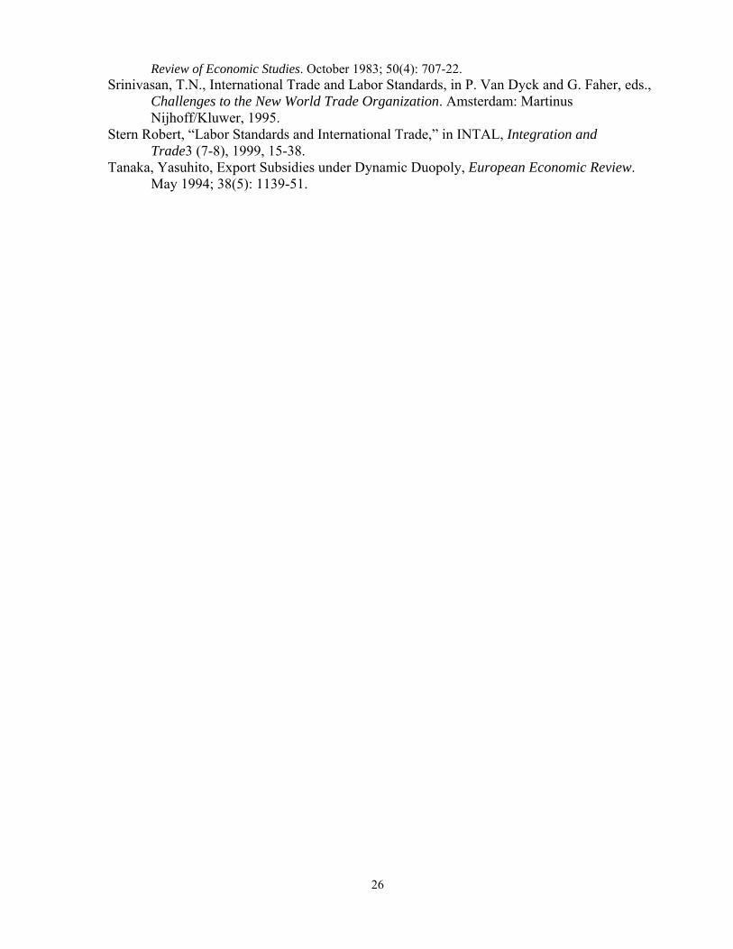
(ii). . In this case, LS produced in the first period is spilled over to the

second period. For sufficient small w, continuous best response curves are still available

(Figure 3). The difference from case (i) is that with LS spillovers, the home best response

curve reaches a vertical line rather than the vertical axis.

1, 0wδ < >

21[(1 ) ]A δ θ−

3 The best response of the home firm jumps to when 2 0y = *2 2( ( ) / 6 )w g a s y A= + − , and stays there

thereafter. Similarly, for δ<1 and relatively large w>0, such jumps are possible. Even if jumping occurs, the existence of Nash equilibrium can still be ensured if w is not too large.

10

Continuity, concavity and the relative position of the two best response curves in

Figure 2 reveal that a unique, stable Nash equilibrium exists in the present model. When the

LS spillover is small, the relative position of the two best response curves in Figure 3 is

similar to in Figure 2. That is, a unique, stable Nash equilibrium still exists.

As for the first period, similar analysis applies. And for the existence, uniqueness and

stability of the Nash Equilibrium in plane, see Appendix 1. *2 , θ θ2

3.1 Comparative Statics in the Second Period

Total differentiation of (7b) yields respectively,

2

2

0sθ∂

>∂

, (9a)

2

2

0θσ∂

>∂

, (9b)

2*2

0yθ∂

<∂

, (9c)

Conditions (9a) and (9b) say that an increase in either home output subsidy or LS subsidy in

the second period raises home LS in the same period. Alternatively, for given and , an

increase in or increases the value of function (defined in (8)), which leads to a

higher . Combined with (7a), it implies that both subsidies raise the home production of

the final output. These are illustrated by an upward shift of the home firm’s best response

curve in Figure 3, moving the equilibrium from point to . Condition (9c) states that an

increase in foreign output in the second period reduces home LS (a lower value of ),

α w

2(θ

2s 2σ 2( )g θ

0E

2θ

sE

)g

11

leading to a lower home output. Incorporating the interpretations of (9a) and (9b), this further

implies that foreign subsidy either on output or LS reduces home production of the final

output in the same period.

4. Inter-temporal Analysis

In the first period, the two firms maximize their respective inter-temporal profits

simultaneously. The home firm’s inter-temporal profits can be written as

, (10)

*1 1 1 2 2 1 2 1 1 1 1 1 1 1 1

*1 2 2 2 2 2 2 2 2 1 2

( , ) ( ( ), ) {( ) } (1 )

[{( ) } (1 ) ( ) ]

y y y y

y y y y

L L L L L a s y L L wL

wL a s y L L wL L wL

θ θ θ θ

θ θ

π γπ θ θ ασ

γ θ θ ασ

Π = + = + − − − −

− + + − − − − −

where is an exogenous discount rate. Each firm maximizes (10) with respective to and

. By the envelope theorem, the first order conditions are obtained as

γ 1Lθ

1yL

*1 1 1 1 1 1 2

1

0 : {( ) 2 } [1 (1 )] [ (1 ) ] 0y ya s y L L w wLθ

θ α γ δ σ γ δ σ α∂Π= + − − − − − + − −

∂= ,(11a)

*1 1 1 1 1

1

0 : {( ) 2 } 0yy

a s y L wL

θ θ∂Π= + − − −

∂= , (11b)

which can be combined to yield:

11 1{[1 (1 )] [ (1 ) ] }yL θγ δ σ γ δ σ α

α= − − − − − 2 , (12a)

3

*11 2 1 1 1

2 {[1 (1 )] [ (1 ) ] } ( ) 0a s y wθ γ δ σ γ δ σ α θα

− − − − − − + + − − = . (12b)

12

In a one-period model, , and condition (12a) collapses to (7a). However, due to

the spillover effect in a two-period model, , and condition (12a) says that the firm over

produces LS in the first period, from the point of maximizing single-period profits.

1δ =

1δ <

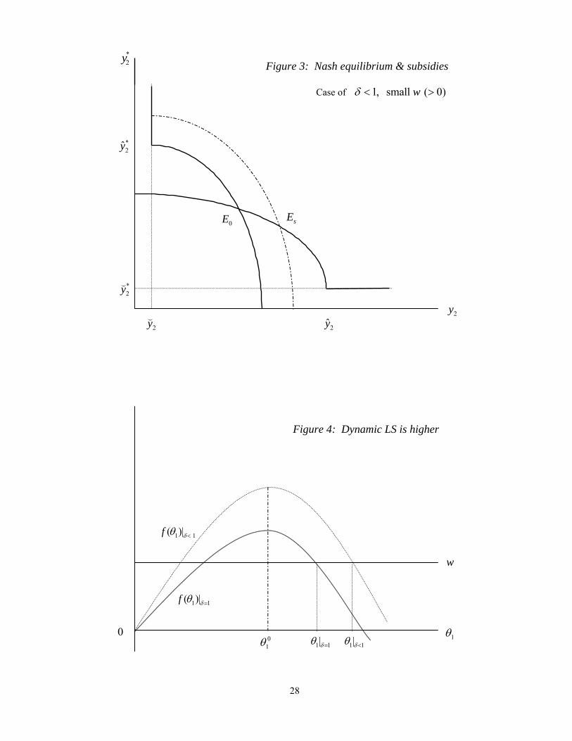
Just as in (7b), there exists one unique solution satisfying condition (12b). Let us

define the first two terms on the LHS of (12b) to be:

3

*11 1 2

2( ) {[1 (1 )] [ (1 ) ] } ( )f aθθ γ δ σ γ δ σ αα

= − − − − − − + + −1 1 1s y θ . (12b’)

Figure 4 illustrates the situation. The static case corresponds to . When the spillover

rate 1 increases (i.e., decreases from ), curve shifts up, resulting in a

higher . Therefore, we can establish:

1δ =

)δ−

1θ

δ 1δ = 1(f θ

Proposition 1: The first-period LS in a dynamic setup is higher than the static LS.

Since the second-period LS is identical to the static one, Proposition 1 thus implies

that the average LS maintained across periods is higher than the static one.

4.1 Inter-temporal Comparative Statics

Total differentiation of (12b) yields respectively

1

1

0sθ∂

>∂

, (13a)

1

1

0θσ∂

>∂

, (13b)

13

1*1

0yθ∂

<∂

, (13c)

1

2

0θσ∂

<∂

, (13d)

2

1

0θσ∂

<∂

. (13e)

In deriving the above, we have used the second order condition,

2 2 221 1 1

2 21 1 1 1

( )( ) ( )y yL L L Lθ θ

π π π∂ ∂ ∂−

∂ ∂ ∂ ∂0> , which is equivalent to 1

1

( ) 0f θθ

∂>

∂.

The interpretations of conditions (13a), (13b) and (13c) are similar to (9a), (9b) and

(9c). Basically, an increase in either home output subsidy or LS subsidy raises home LS in

the same period, leading to a higher home final output. Foreign subsidies would have

opposite effects on home variables in the same period. In Figure 4, an increase in either or

causes curve to shift up, resulting in a higher , while an increase in either or

does the opposite.

1s

*1y1σ

2σ

1( )f θ 1θ

Condition (13d) states that an increase in home LS subsidy in the second period

reduces home LS in the first period, because the firm expects to receive subsidy in the second

period, and thus it under produces LS in the first period. This in turn reduces home output but

raises foreign output in the first period.

Next, we are interested in how first-period subsidies affect second-period variables.

Condition (13e) says that first-period subsidy on LS reduces second period-production of LS.

Even though an increase in first-period subsidy does not affect the total LS used in the

14

second period according to (7b), because an increase in raises in (13b), it follows

that must fall.

2θ 1σ 1θ

2θ

By Lemma 1, second-period LS is chosen independently of first-period subsidies, i.e.,

the latter does not have any effects on second-period LS and output. However, since first-

period subsidies raise , which in turn reduces labor input to produce LS in the second

period , the home firm gains by saving on . Therefore, the home firm’s profit

increases, even though its output remains unaffected by first-period subsidies.

1θ

2Lθ 2Lθ

How do first-period home subsidies affect second-period foreign variables? We

already know that foreign LS and output fall as a consequence of home subsidies in either

form in the first period. This in turn leads to a lower foreign LS that is spilled over in the

second period. Even though foreign output is not changed, the foreign firm must input more

, to maintain an optimal LS. Thus, cost increases and profit falls in the second period. *2Lθ

The above can be summarized as

Proposition 2: First-period home subsidy on either output or LS increases (decreases)

second—period home (foreign) profits.

5. Optimal Subsidies

In this section, we investigate the governments’ optimal subsidies. We hope to make

clear whether it is better for governments to subsidize output or LS production; whether to

subsidize in the first period, or in the second period; and compare them with static subsidies.

Since final sales of the good are in a third-country market, each country’s welfare is the sum

of profits in the two periods, subtracted by the sum of subsidies; that is,

15

. (14)

* *1 1 1 1 1 1 2 2 2 2 2 2

1 1 1 1 2 2 2 2

( , ; , , ) ( , ; , , )

[ ]

y ys L L y s L L y

s y w s y w

θ θπ σ γπ σ

σ θ γ σ θ

Φ = +

− − − +

Differentiation of (14) yields respectively

*

111 1 1 1 1 11 1 1*

1 1 1 1 1 1 1 1 1

y

y

LL y yy s ws L s L s y s s s s

θ

θ

π π π π σ∂∂∂ ∂ ∂ ∂ ∂ ∂∂Φ

= + + + − − −∂ ∂ ∂ ∂ ∂ ∂ ∂ ∂ ∂ ∂

1

1

θ∂, (15a)

*

222 2 2 2 2 22 2 2*

2 2 2 2 2 2 2 2 2

( )y

y

LL y yy s ws L s L s y s s s s

θ

θ

π π π π σγ

∂∂∂ ∂ ∂ ∂ ∂ ∂∂Φ= + + + − + +

∂ ∂ ∂ ∂ ∂ ∂ ∂ ∂ ∂ ∂2

2

θ∂, (15b)

*

111 1 1 1 1 1 11 1 1 2*

1 1 1 1 1 1 1 1 1 1

y

y

LL y ys w w wL L y

θ

θ

π π π π θθ σ γσσ σ σ σ σ σ σ

∂∂∂ ∂ ∂ ∂ ∂ ∂ ∂∂Φ= + + + − − − −

∂ ∂ ∂ ∂ ∂ ∂ ∂ ∂ ∂ ∂ ∂2

1

θσ∂

,(15c)

21 21 1 21

2 1 2 2 2 2 2

*2 2 2 2 2

2 2 2*2 2 2 2 2

{

( )}

y

y

LL LwL L

y yw s wy

θ θ

θ θ

π θ π πσ γσ σ σ σ

π π θθ σσ σ σ σ

∂∂ ∂∂ ∂ ∂ ∂∂Φ= − + +

∂ ∂ ∂ ∂ ∂ ∂ ∂ ∂

∂ ∂ ∂ ∂ ∂+ + − + +∂ ∂ ∂ ∂ ∂

2

2L σ

. (15d)

Letting all these equal to zero, and using the envelope theorem, substitution gives rise to

respectively

*

1 1 1 11 1 1

1 1 1 1

(1 ) { } 0y yw w s ys s s sθ θγ δ σ

α∂ ∂ ∂ ∂

− − − + + =∂ ∂ ∂ ∂

, (15a’)

*

2 2 22 2 2

2 2 2

{ y yw s ys s sθσ ∂ ∂ ∂

− + +∂ ∂ ∂

} 0= , (15b’)

16

*

1 1 1 1 21 1 1 2

1 1 1 1

(1 ) { } 0y yw w s y wθ θ θγ δ σ γσα σ σ σ σ σ

∂ ∂ ∂ ∂ ∂− − − + + − =

∂ ∂ ∂ ∂ ∂ 1

, (15c’)

*

11 1 2 21 2 2 2

1 2 2 2 2 2

{L y yw w s yL

θ

θ

π θ θσ σσ σ σ σ σ∂∂ ∂ ∂ ∂ ∂

− − + +∂ ∂ ∂ ∂ ∂ ∂

2 } 0= . (15d’)

Some explanations are in order. Condition (15b’) is identical to the case of static

subsidies, implying that the optimal subsidy on output in the second period is equal to the

static one. Suppose that the government initially does not subsidize LS, i.e. , then

(15b’) can be rewritten as

2 0σ =

*2 2

2 22 2

/y ys ys s∂ ∂

= − >∂ ∂

0 . (15b’’)

That is, the optimal subsidy on output is positive. Furthermore, for a small subsidy on LS, i.e.

as increases slightly above zero, such that and hold, the optimal subsidy

on output is still positive according to (15b’). Analogously, this result arises again in the

curled brackets in (15d’). Thus we can state

2σ 2 0σ > 2 0σ ≈

Proposition 3: When the government subsidizes LS and output simultaneously, both

subsidies are positive in a static setup.

Proposition 3 is in stark contrast to Spencer and Brander (1983), who show that when both

subsidies on R&D and output are available, the former is negative while the latter is positive

(Proposition 4). Their contrasting results arise because of two reasons: One is that increases

in R&D reduce the unit cost of production, while increases in output raise the cost of

production; The other is that R&D is conducted in a stage prior to production, such that R&D

17

has a strategic effect of increasing production, which leads the firm to over-invest in R&D,

resulting in a distortion. In order to correct the distortion, the government taxes R&D

activities and subsidizes production.

In contrast, in the present model, LS and final production are done simultaneously, thus

there is no strategic effect or distortion. In addition, as shown in (2), labor input for LS

and labor input for production enter symmetrically in final production. A subsidy on one

increases the marginal product of the other. Thus, Proposition 3 is obtained.

Lθ

yL

Next, we investigate condition (15a’), which has one more term than (15b’) does, i.e., the

first term on the LHS of (15a’), 1 1 1

1 1 1

(1 ) 0ws L sθ

θ π θγ δα α

∂ ∂ ∂− − = <

∂ ∂ ∂, using condition (13a) and

1

1

0Lθ

π∂<

∂. (16)

Condition (16) holds because the firm over invests in , which can be spilled over and re-

used in period two. An increase in output subsidy in the first period further enlarges the

effect in (16). The government takes this into consideration when choosing subsidies.

Therefore, the optimal subsidy to output in the first period is less than the static one.

1Lθ

We are now in a position to state the results above as:

Proposition 4: In a dynamic setup, (i). The second-period subsidy on output is positive; (ii).

The first-period subsidy on output is lower than the static (or second-period) subsidy.

Analogously, the first two terms on the LHS in condition (15c’) are similar to

condition (15a’), which lowers the optimal subsidy to LS in the first period, since the firm

over invests in due to the spillover effect. However, there is an additional term after the 1Lθ

18

curled brackets, which is positive by condition (9d). This is again due to the spillover effect.

It works as follows: the subsidy on LS in the first period lowers the second-period production

of LS, which helps the firm to save investment cost. Summing up, there are two additional

effects of first-period subsidy compared to a static subsidy. One lowers the subsidy on LS,

but the other one raises it. Note that under the subsidy on output, the latter effect is absent.

Therefore we can conclude that subsidy is more effective on LS than on output in the first

period.

In condition (15d’), the term in the curled brackets is identical to the condition

determining the optimal static subsidy on LS. The two terms before that are both positive,

using condition (16) and (13d). They capture two effects of raising the second period subsidy

on LS. One is that since the firm over invests in LS, it lowers the marginal profit in the first

period by (16). The subsidy in the second period weakens this effect by inducing inter-

temporal trade-offs so that the firm produces less LS in the first period and more in the

second period; The other is that raising second-period subsidy on LS reduces first period LS,

which saves LS subsidy expenditure for the government in the first period. These imply that

second-period subsidy on LS is higher than the static one.

Summarizing the above, we can state:

Proposition 5: In a dynamic setup, (i). First period subsidy is more effective on LS than on

output; (ii). Second-period subsidy on LS is higher than the static subsidy.

6. Human Rights Concerns

Labor unions, human rights groups and other NGOs in developed countries are

concerned about human rights and social justice in developing countries. They argue that 19

firms able to adopt a lower LS gain a competitive edge, and thus some even advocate for

trade sanctions against countries that do not enforce a set of agreed LS.

Following such popular claims that governments in developed countries also care

about LS (or human rights) in developing countries, in this section, we suppose that

government utility increases if LS in the other country rises. Hence, the home government’s

objective function can now be written as:

, (16) * * *1 1 1 1 1 2 2 2 2 2 1 2( , ; , , ; , ; , , ) { ( ) ( )}y ys L L y s L L y h hθ θσ σ θ γΨ = Φ + + *θ

where Φ is given in (14), and represents how foreign LS affects home government

objectives, with h Home LS does not enter the objective function directly

because LS in developed countries has reached a certain threshold level, enabling the

government not to worry about it.

( )h θ

.<' 0, " 0h>

The first order conditions to maximize (16) are respectively,

* *1 2

1 1 1 1

( )hs s s s

θ θγ∂ ∂∂Ψ ∂Φ= + + =

∂ ∂ ∂ ∂' 0 , (17a)

* *2 1

2 2 2 2

( )hs s s s

θ θγ ∂ ∂∂Ψ ∂Φ= + + =

∂ ∂ ∂ ∂' 0 , (17b)

* *1 2

1 1 1 1

( )hθ θγσ σ σ σ

∂ ∂∂Ψ ∂Φ= + + =

∂ ∂ ∂ ∂' 0 , (17c)

* *1 2

2 2 2 2

( )hθ θγσ σ σ σ

∂ ∂∂Ψ ∂Φ= + + =

∂ ∂ ∂ ∂' 0 . (17d)

These first order conditions give rise to:

20

Proposition 6: When the home government considers foreign LS (human rights) in its

objective, (i). the optimal subsidies on outputs in both periods and the optimal subsidy on LS

in the first period become lower; (ii). the optimal subsidy on LS in the second period also

becomes lower if and the cross-period effect of the subsidy is lower than the within-

period effect.

1γ ≈

Proof: We only need to examine the terms in the parentheses in the first order conditions.

(i). In conditions (17a), (17b) and (17c), the second terms in parentheses are all equal

to zero, i.e., *2

1

0,sθ∂

=∂

*1

2

0,sθ∂

=∂

and *2

1

0θσ∂

=∂

. Now we examine the first terms. In (17a),

*1

1

0sθ∂

<∂

, because 1

1

0sθ∂

>∂

and *1

1

0θθ

∂<

∂ hold; in (17b),

*2

2

0sθ∂

<∂

because of 2

2

0sθ∂

>∂

,

*2

2

0θθ∂

<∂

and *1

2

0sθ∂

=∂

; and in (17c), obviously *1

1

0θθ

∂<

∂ holds.

(ii). In (17d), the cross-period effect is *1

2

0θσ∂

>∂

, because 1

2

0θσ∂

<∂

and *1

1

0θθ

∂<

∂ hold.

However, the within-period effect is *2

2

0θσ∂

<∂

. These two effects work against each other.

Under the conditions that and that the cross-period effect of the subsidy is lower than

the within-period effect, then the sum of the terms in parentheses becomes negative.

1γ ≈

In summary, incorporating foreign LS adds only negative terms to the first order

conditions of the government’s maximization problem, reducing the optimal subsidies.

QED

21

Proposition 6 implies that if the home government cares about LS in a developing

country, then home subsidies on either output or LS, in either period, would reduce foreign

LS, eventually leading to lower welfare in the home country.

7. Concluding Remarks

This paper has modeled productive labor standards in a two-stage, two-period model

of international oligopoly, where governments choose subsidies on LS and output first, and

oligopolistic firms determine production of LS and output later. Under productive LS, “a

race to the bottom” of LS does not arise. Even in poor countries, maintaining a certain level

of LS is beneficial to the workers, the firms and national welfare there. Furthermore, this

effect becomes even stronger in a dynamic setting where LS upgraded today contributes to

production tomorrow.

We also showed that the optimal subsidies on LS and output are positive. While

second-period output subsidy is equal to the static one, second-period LS subsidy is higher

than the static one. And with inter-temporal LS spillovers, subsidies are more effective on LS

than on output. If the home government cares about LS (or human rights) in the foreign

country, then it is better not to provide home subsidies on either LS or output, because such

subsidies reduce foreign LS.

We have assumed that firms compete in quantity in the goods market. They could

also compete in prices. It is well known that prices are lower and outputs higher under price

competition than under quantity competition (see for instance, Cheng, 1985), and that export

taxes rather than subsidies may be called for (Eaton and Grossman, 1986).

22

8. Appendix 1 Existence, uniqueness and stability of the Nash Equilibrium in plane *2 , θ θ2

We start the proof with the case of and . As shown in Section 3, for any

, there exists a unique solution of (7b), , which constitutes the best response

curve of the home firm, in the range

1δ = 0w =

)*2 0θ ≥ *

2 2(θ θ

*),θ θ * ]2 2θ θ 2 2( )[ ( . Differentiating the boundaries yield

respectively *2 2/ 0θ θ <∂ ∂ , *

2 2/ 0θ θ <∂ ∂ , 2 /( * 2) 0<2 2θ θ∂ ∂ and 2 * 22 2/( ) 0θ θ <∂ ∂ , i.e., the

boundary loci are downward sloping and concave to origin. The area enclosed by the two

boundary loci, *2 2(θ θ ) and *

2 2(θ θ ) , constitutes the feasible region in which the best response

curve lies. For the home firm, the two boundary loci intersect at

* *hom 2( 0) | ( ) /e a s A= = +

*2θ

2 2θ θ , where . At this point, the best response

curve intersects with the axis. For any , always holds along the

best response curve.

* * 1( ) (1α −=

* *2 2θ θ

*2α−

hom( 0)θ> =

*)σA

|2 e 2 0θ =

Now, differentiating the best response function in (7b) gives rise to,

* ** 2 2

2 22/ 0A θ θθ θ∂ ∂ = <

∆, and

2 ** * *2 22 2 22* 2

2

2 [ 4 24 /( )

A y AAθ θ θ θθ∂

= ∆ + −∆∂

0 *2 2 22y a s y< + −

]∆ , where

. Since , we have *2 2 2( ) 6a s y y∆ = + − − <

22

* 22

0( )

θθ∂

>∂

in the neighborhood

of . That is, the best response curve is continuous, downward sloping, and convex to

the origin. The foreign firm’s best response curve can be constructed in a similar fashion.

*2 2y y≈

The points at which the best response curves hit the horizontal axis can be derived as,

*2 2 hom 2( 0) | ( ) /(2e a s Aθ θ = = + ) and * *

2 2 2( 0) | ( ) /foreign a s Aθ θ = = +

* *2 hom 2 2( 0) | ( 0) |e foreignθ θ= < =

, where A .

In the neighborhood of , holds, i.e., the foreign

firm’s best response curve hits the horizontal axis to the right of the home best response

12(1 )α ασ−= −

*2 2s s≈ 2θ θ

23

curve. Analogously, , the foreign firm’s best response curve

hits the vertical axis below the point when the home firm’s best response curve hits the

vertical axis. Continuity guarantees that the two curves meet at least once. And convexity of

the two curves ensures that their intersection occurs at most once. Therefore, we obtain a

unique Nash equilibrium, which is stable due to the relative position between them.

* *2 2 hom 2 2( 0) | ( 0) |eθ θ θ θ= > =

1δ <

(0,0) 1((1 ) , (1δ θ−

( 0)w >

foreign

1

In the more general case of and a small , we set (( as

the origin point rather than , since is the LS spilled over from the

first period. Then for sufficiently small , we still obtain continuous best response

curves as above.

( 0)w >

*) )δ θ−

*1 11 ) , (1 ) )δ θ δ θ− −

Similar to section 3 (footnote 3), when w is sufficiently large, there is a possibility

that the best response curves become discontinuous, and a Nash equilibrium may not exist.

24

References

Bagwell, Kyle, and R. W. Staiger, The WTO as a Mechanism for Securing Market Access Property Rights: Implications for Global Labor and Environmental Issues, Journal of Economic Perspectives 15, 3, 2001, 69-88.

Basu, Kaushik, International Labor Standards and Child Labor, Challenge, v42, n5, 1999, 80-93. Basu, Kaushik and Van, Pham Hoang, The Economics of Child Labor, American-Economic-Review.

June 1998; 88(3): 412-27. Benchekroun, Hassan, Unilateral Production Restrictions in a Dynamic Duopoly, Journal of

Economic Theory. August 2003; 111(2): 214-39. Bhagwati, Jagdish, Trade Liberalization and ‘Fair Trade’ Demands: Addressing

Environmental and Labor Standards Issues, World Economy 18, 1995. Brander, James A and Spencer, Barbara J., Export Subsidies and International Market Share Rivalry,

Journal of International Economics. February 1985; 18(1-2): 83-100. Brown, D. K., Labor standards, where do they belong on the international trade agenda?

Journal of Economic Perspectives 15(3), 2001, 89-112. Brown, D. K., Alan V. Deardorff and Robert M. Stern, International Labor Standards and

Trade: A Theoretical Analysis, in J. Bhagwati and R. Hudec, eds., Fair Trade and Harmonization: Prerequisites for Free Trade? Economic Analysis, Vol. 1, Cambridge and London: MIT Press, 1996, 227-80.

Brown, D. K., Alan V. Deardorff and Robert M. Stern, Trade and Labor Standards, Open Economies Review. April 1998; 9(2): 171-94.

Cheng, Leonard, Comparing Bertrand and Cournot Equilibria: A Geometric Approach, Rand

Journal of Economics 16, 1985, 146-52. Eaton, Jonathan and Gene Grossman, Optimal Trade and Industrial Policy under Oligopoly,

Quarterly Journal of Economics 101, 1986, 383-406. Elliot, Kimberly, Ann., Preferences for Workers? Worker Rights and the US Generalized

System of Preference, 2000. Hussain, Mahmood and Keith Maskus, Child Labor Use and Economic Growth: An

Economeric Analysis, World Economy, July 2003; 26(7): 993-1017. Itaya, Jun-Ichi, Dynamic Tax Incidence in a Finite Horizon Model, Public Finance. 1995;

50(2): 246-66. Jafarey, Saqib, and Sajal Lahiri, Will Trade Sanctions Reduce Child Labour? The Role of Credit

Markets, Journal of Development Economics. June 2002; 68(1): 137-56. Martin, William J. and Keith Maskus, The Economics of Core Labor Standards: Implications

for Global Trade Policy," Review of International Economics, Vol. 9, No. 2, May 2001, 317-328.

Ohkawa, Takao and Koji Shimomura, Dynamic Effects of Subsidies on Outputs and R&D in an International Export Rivalry Model, in W. Chang and S. Katayama (eds.) Imperfect Competition in International Trade, Kluwer Acamadic Publishers, 1995, 175-84.

Ranjan, P., Credit Constraints and the Phenomenon of Child Labor, Journal of Development Economics 64, 2001, 81-102.

Rodrik, Dani, "Labor Standards in International Trade: Do They Matter and What Do We Do About Them?" in R. Lawrence et al., Emerging Agenda for Global Trade: High Stakes for Developing Countries, Overseas Development Council, Washington, DC, 1996.

Spencer, Barbara J. and Brander, James A, and International R & D Rivalry and Industrial Strategy.

25

Review of Economic Studies. October 1983; 50(4): 707-22. Srinivasan, T.N., International Trade and Labor Standards, in P. Van Dyck and G. Faher, eds.,

Challenges to the New World Trade Organization. Amsterdam: Martinus Nijhoff/Kluwer, 1995.

Stern Robert, “Labor Standards and International Trade,” in INTAL, Integration and Trade3 (7-8), 1999, 15-38.

Tanaka, Yasuhito, Export Subsidies under Dynamic Duopoly, European Economic Review. May 1994; 38(5): 1139-51.

26

2θ

2( )g θ

w

02

2θ2θ

1, 0wδ = =

0E*2

6a s+

2a s+

*2

2a s+

*2y

2

2a s+

2

6a s+

27

Figure 2:

y*2a s+

Home best response

Foreign best response

θ

Figure 1: Optimal

2

1, small ( 0)wδ < >

Figure 3: Nash equilibrium & subsidies

Case of

*2y

*2y

*y

0E sE

28

2y2

2y2y

Figure 4: Dynamic LS is higher

1 1( )|f δθ <

1 1|δθ <

1 1( )|f δθ =

1 1|δθ =

00

1θ

1θ

w