dynamic data fusion for future sensor networks

Dynamic Data Fusion for Future Sensor Networks

Umakishore Ramachandran, Rajnish Kumar, Matthew Wolenetz, Brian Cooper,

Bikash Agarwalla, JunSuk Shin, Phillip Hutto, and Arnab Paul

College of Computing,

Georgia Institute of Technology

DFuse is an architectural framework for dynamic application-specified data fusion in sensornetworks. It bridges an important abstraction gap for developing advanced fusion applicationsthat takes into account the dynamic nature of applications and sensor networks. Elements of theDFuse architecture include a fusion API, a distributed role assignment algorithm that dynamicallyadapts the placement of the application task graph on the network, and an abstraction migrationfacility that aids such dynamic role assignment. Experimental evaluations show that the APIhas low overhead, and simulation results show that the role assignment algorithm significantlyincreases the network lifetime over static placement.

Categories and Subject Descriptors: D.4.7 [Operating Systems]: Organization and Design –Distributed Systems, and Embedded Systems

General Terms: Algorithms, Design, Management, Measurement

Additional Key Words and Phrases: Sensor Network, In-network aggregation, Data fusion, Roleassignment, Energy awareness, Middleware, Platform

1. INTRODUCTION

There is an ever-evolving continuum of sensing, computing, and communicationcapabilities from smartdust, to sensors, to mobile devices, to desktops, to clusters.With this evolution, capabilities are moving from the larger footprint to the smallerfootprint devices. For example, tomorrow’s mote will be comparable in resourcesto today’s mobile devices; and tomorrow’s mobile devices will be comparable tocurrent desktops. These developments suggest that future sensor networks maywell be capable of supporting applications that require resource-rich support today.Examples of such applications include streaming media, surveillance, image-basedtracking and interactive vision. Many of these fusion applications share a commonrequirement, namely, hierarchical data fusion, i.e., applying a synthesis operationon input streams.

Authors emails: {rama, rajnish, wolenetz, cooperb, bikash, espress, pwh, arnab}@cc.gatech.edu

The work has been funded in part by an NSF ITR grant CCR-01-21638, NSF grant CCR-99-72216, HP/Compaq Cambridge Research Lab, the Yamacraw project of the State of Georgia, andthe Georgia Tech Broadband Institute. The equipment used in the experimental studies is fundedin part by an NSF Research Infrastructure award EIA-99-72872, and Intel Corp.Permission to make digital/hard copy of all or part of this material without fee for personalor classroom use provided that the copies are not made or distributed for profit or commercialadvantage, the ACM copyright/server notice, the title of the publication, and its date appear, andnotice is given that copying is by permission of the ACM, Inc. To copy otherwise, to republish,to post on servers, or to redistribute to lists requires prior specific permission and/or a fee.c© 20XX ACM 1529-3785/20XX/0700-0100 $5.00

ACM Transactions on Sensor Networks, Vol. X, No. Y, XX 20XX, Pages 100–0??.

· 101

This paper focuses on the challenges involved in supporting fusion applicationsin wireless ad hoc sensor networks (WASN). Developing a fusion application ischallenging in general, for the fusion operation typically requires time-correlationand synchronization of data streams coming from several distributed sources.

Since such applications are inherently distributed, they are typically implementedvia distributed threads that perform fusion hierarchically. Thus, the applicationprogrammer has to deal with thread management, data synchronization, bufferhandling, and exceptions (such as time-outs while waiting for input data for afusion function) - all with the complexity of a loosely coupled system. WASNadd another level of complexity to such application development - the need forbeing power-aware [Cayirci et al. 2002]. In-network aggregation and power-awarerouting are techniques to alleviate the power scarcity of WASN. While the goodnews about fusion applications is that they inherently need in-network aggregation,a naive placement of the fusion functions on the network nodes will diminish theusefulness of in-network fusion, and reduce the longevity of the network (and hencethe application). Thus, managing the placement (and dynamic relocation) of thefusion functions on the network nodes with a view to saving power becomes anadditional responsibility of the application programmer. Dynamic relocation maybe required either because the remaining power level at the current node is goingbelow a threshold, or to save the power consumed in the network as a whole byreducing the total data transmission. Supporting the relocation of fusion functionsat run-time has all the traditional challenges of process migration [Zayas 1987].

We have developed DFuse, an architecture for programming fusion applications.It supports distributed data fusion with automatic management of fusion pointplacement and migration to optimize a given cost function (such as network longevity).Using the DFuse framework, application programmers need only implement the fu-sion functions and provide the dataflow graph (the relationships of fusion functionsto one another, as shown in Figure 1). The fusion API in the DFuse architec-ture subsumes issues such as data synchronization and buffer management that areinherent in distributed programming.

The main contributions of this work are summarized below:

(1) Fusion API: We design and implement a rich API that affords programmingease for developing complex sensor fusion applications. The API allows anysynthesis operation on stream data to be specified as a fusion function, rangingfrom simple aggregation (such as min, max, sum, or concatenation) to morecomplex perception tasks (such as analyzing a sequence of video images). Thisis in contrast to current in-network aggregation approaches [Madden et al. 2002;Intanagonwiwat et al. 2000; Heidemann et al. 2001] that allow only limited typesof aggregation operations as fusion functions. The API includes primitives foron-demand migration of the fusion point.

(2) Distributed algorithm for fusion function placement and dynamic relocation:There is a combinatorially large number of options for placing the fusion func-tions in the network. Hence, finding an optimal placement, in a distributedmanner, that minimizes communication is difficult. We develop a novel heuristic-based algorithm to find a good (with respect to some predefined cost function)mapping of fusion functions to the network nodes.

ACM Transactions on Sensor Networks, Vol. X, No. Y, XX 20XX.

102 ·

Also, the placement needs to be re-evaluated quite frequently considering thedynamic nature of WASN. The mapping is re-evaluated periodically to addressdynamic changes in nodes’ power levels and network behavior.

Fusion and aggregation terms are often used interchangeably in sensor networkcommunity. For clarification, however, we would like to note down a basicdifference. An aggregation is typically performed on data of same type, tominimize communication; while a fusion is performed on data of possibly dif-ferent types, to derive a decision. Thus, a fusion point placement is a moreconstrained problem than an aggregator placement.

(3) Experimental evaluation of the DFuse framework: The evaluation includesmicro-benchmarks of the primitives provided by the fusion API as well as mea-surement of the data transport in a tracker application. Using an implementa-tion of the fusion API on a wireless iPAQ farm coupled with an event-drivenengine that simulates the WASN, we quantify the ability of the distributed al-gorithm to increase the longevity of the network with a given power budget ofthe nodes. For example, we show that the proposed role assignment algorithmincreases the network lifetime by 110% compared to static placement of thefusion functions.

(4) Simulation results for larger networks: Using a novel middleware simulator(MSSN) [Wolenetz 2005; Wolenetz et al. 2004; 2005], we simulate the DFusearchitecture on a network of hundreds of nodes and for different sizes of theapplication task graph. We show that the performance of DFuse scales well forlarger networks and application graphs with respect to an optimal placement(approximated using a simulated annealing algorithm).

This journal version of the paper is a significant extension of a previous conferencepublication [Kumar et al. 2003]. The extensions are along the following dimensions:1) We present a comprehensive list of the APIs available in the fusion module. 2) Weintroduce the bottom-up and top-down approaches to improving the quality of theinitial placement of the role assignment algorithm. Based on the characteristic ofthe input task graph, one or the other approach may be more desirable to providea better initial deployment. 3) Using a novel home-grown middleware simulator(MSSN), we present scalability results in terms of increase in network size as wellas in the size of the input application task graph. Within the simulator, we havedeveloped approximations to an optimal assignment (using simulated annealingalgorithm) that allows comparison of our proposed role assignment algorithm to atheoretical optimal.

The rest of the paper is structured as follows. Section 2 analyzes fusion applica-tion requirements and presents the DFuse architecture. In Section 3, we describehow DFuse supports distributed data fusion. Section 4 explains a heuristic-baseddistributed algorithm for placing fusion points in the network. This is followed byimplementation details of the framework in Section 5 and its evaluation in Section 6.We then compare our work with existing and other ongoing efforts in Section 7,present some directions for future work in Section 8, and conclude in Section 9.


· 103

2. APPLICATION CONTEXT AND REQUIREMENTS

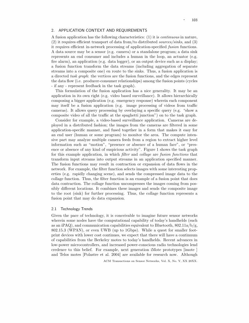
A fusion application has the following characteristics: (1) it is continuous in nature,(2) it requires efficient transport of data from/to distributed sources/sinks, and (3)it requires efficient in-network processing of application-specified fusion functions.A data source may be a sensor (e.g. camera) or a standalone program; a data sinkrepresents an end consumer and includes a human in the loop, an actuator (e.g.fire alarm), an application (e.g. data logger), or an output device such as a display;a fusion function transform the data streams (including aggregation of separatestreams into a composite one) en route to the sinks. Thus, a fusion application isa directed task graph: the vertices are the fusion functions, and the edges representthe data flow (i.e. producer-consumer relationships) among the fusion points (cycles- if any - represent feedback in the task graph).

This formulation of the fusion application has a nice generality. It may be anapplication in its own right (e.g. video based surveillance). It allows hierarchicallycomposing a bigger application (e.g. emergency response) wherein each componentmay itself be a fusion application (e.g. image processing of videos from trafficcameras). It allows query processing by overlaying a specific query (e.g. “show acomposite video of all the traffic at the spaghetti junction”) on to the task graph.

Consider for example, a video-based surveillance application. Cameras are de-ployed in a distributed fashion; the images from the cameras are filtered in someapplication-specific manner, and fused together in a form that makes it easy foran end user (human or some program) to monitor the area. The compute inten-sive part may analyze multiple camera feeds from a region to extract higher levelinformation such as “motion”, “presence or absence of a human face”, or “pres-ence or absence of any kind of suspicious activity”. Figure 1 shows the task graphfor this example application, in which filter and collage are fusion functions thattransform input streams into output streams in an application specified manner.The fusion functions may result in contraction or expansion of data flows in thenetwork. For example, the filter function selects images with some interesting prop-erties (e.g. rapidly changing scene), and sends the compressed image data to thecollage function. Thus, the filter function is an example of a fusion point that doesdata contraction. The collage function uncompresses the images coming from pos-sibly different locations. It combines these images and sends the composite imageto the root (sink) for further processing. Thus, the collage function represents afusion point that may do data expansion.

2.1 Technology Trends

Given the pace of technology, it is conceivable to imagine future sensor networkswherein some nodes have the computational capability of today’s handhelds (suchas an iPAQ), and communication capabilities equivalent to Bluetooth, 802.11a/b/g,802.15.3 (WPAN), or even UWB (up to 1Gbps). While a quest for smaller foot-print devices with lower cost continues, we expect that there will have a continuumof capabilities from the Berkeley motes to today’s handhelds. Recent advances inlow-power microcontrollers, and increased power-conscious radio technologies lendcredence to this belief. For example, next generation iMote prototypes [imote ]and Telos motes [Polastre et al. 2004] are available for research now. Although


104 ·

Sink (Display)

Camera Sesnors

Filter

Collage

1

2

3

6 2x

x

2x

x 3x

<TaskGraph name="tracking"> <FusionRole name="filter">

<input name="source" id="1"/> <input name="source" id="2"/> <output name="collage" id="unknown"/>

</FusionRole> <FusionRole name="collage">

<input name="filter" id="unknown"/> <input name="source" id="3"/> <output name="display" id="6"/>

</FusionRole> </TaskGraph>

(A) (B)

Fig. 1. An example application. (A) pictorial representation of the task graph(with expected data flow rates on the edges); (B) textual representation of the taskgraph.

not as computationally powerful as a modern iPAQs, iMotes provide 12MHz 32-bitARM7TDMI processors and 64KB RAM/512KB FLASH, a significant increase incapability compared to Berkeley mote MICA2 [mica2 ] predecessors that only had8MHz 8-bit ATmega128L microcontrollers with 4KB RAM/128KB FLASH. Fur-thermore, the wireless bandwidth available with iMotes is Bluetooth based (over600Kbps application-level bandwidth), greatly exceeding Berkeley motes’ 38.4Kbpsdata rate. Coupled with this trend, high-bandwidth sensors such as cameras arebecoming ubiquitous, cheaper, and lighter (in this case, possibly due to the large-scale demands of cell-phone manufacturers for these cameras, where camera phoneshipment is expected to reach 903 million in 2010 [Reiter ]). Thus, we envision thefuture wireless sensor networks deployments to consist of high bandwidth and pow-erful sensor/actuator sources and infrastructures coexisting with more constrainednodes, with energy still being a scarce resource.

2.2 Architectural Assumptions

We have designed the DFuse architecture to cater to the evolving application needsand emerging technology trends.

We make some basic assumptions about the execution environment in the designof DFuse:

—The application level input to the architecture are:

(1) an application task graph consisting of the data flows and relationship amongthe fusion functions

(2) the code for the fusion functions (currently supported as C program binaries)

(3) a cost function that formalizes some application quality metric for the sensornetwork (e.g. “keep the average node energy in the network the same”).

—The task graph has to be mapped over a large geographical area. In the ensuingoverlay of the task graph on to the real network, some nodes may serve as relayswhile others may perform the application-specified fusion operations.

—The fusion functions may be placed anywhere in the sensor network as long asthe cost function is satisfied.


· 105

—All source nodes are reachable from the sink nodes.

—Every node has a routing layer that allows each node to determine the route toany other node in the network. This is in sharp contrast to most current daysensor networks that support all-to-sink style routing. However, the size of therouting table in every node is only proportional to the size of the application taskgraph (to facilitate any network node in the ensuing overlay to communicate withother nodes hosting fusion functions) and not the physical size of the network.

—The routing layer exposes information (such as hop-count to a given destination)that is needed for making mapping decisions in the DFuse architecture.

It should be noted that dynamically generating a task graph to satisfy a givendata-centric query plan is in itself an interesting research problem. However, thefocus of this paper is to provide the system support to meet the application require-ments elaborated in the previous subsections honoring the above assumptions.

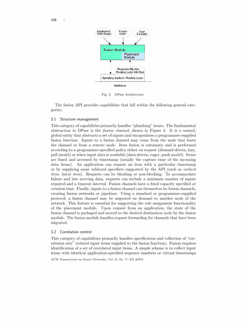
2.3 DFuse Architecture Components

Figure 2 shows the components of the DFuse architecture. There are two com-ponents to this architecture that are the focus of this paper: fusion module, andplacement module.

From an application perspective, there are two main concerns:

(1) How do we develop the fusion application? The fusion code itself (e.g. “motiondetection” over a number of incoming video streams and producing a digest)is in the purview of the application developer. However, there are a numberof systems issues that have to be dealt with before a fusion operation can becarried out at a given node including: (a) providing the “plumbing” from thesources to the fusion point; (b) ensuring that all the inputs are available; (c)managing the node resources (CPU and memory) to enhance performance, and(d) error and failure handling when some sources are non-responsive.We have designed a fusion module with a rich API that deals with all of theabove issues. We describe this module in Section 3.

(2) How do we generate an overlay of the task graph on to the sensor network?As we mentioned earlier, some nodes in the overlay will act as relays and somewill act as fusion points. Since the application is dynamic (sources/sinks mayjoin/leave as dictated by the application, new tasks may be created, etc.), andthe physical network is dynamic (sources/sink may fail, intermediate nodes mayrun out of energy, etc.) this mapping is not a one-time deal. After an initialmapping re-evaluation of the mapping (triggered by changes in the applicationor the physical infrastructure) will lead to new assignment and re-assignmentof the nodes and the roles they play (relay vs. fusion).We have designed a placement module that embodies a role assignment algo-rithm that deals with the above issues. We describe this module in Section 4.

3. FUSION MODULE

The API provided by the fusion module is summarized in Figure 3. The API callsare presented in an abstract form to elide language and platform implementationdetails.


106 ·

� � � � � � �� ! � " � � #� � � � �� $ � % � � �� &� � � � � � � � � � � '� � � � ( � $ �

) � � * �$ � � �� + � � , - � � � . / � � �� 0 � � � 0 � � �/ � � $ � ��

Fig. 2. DFuse Architecture

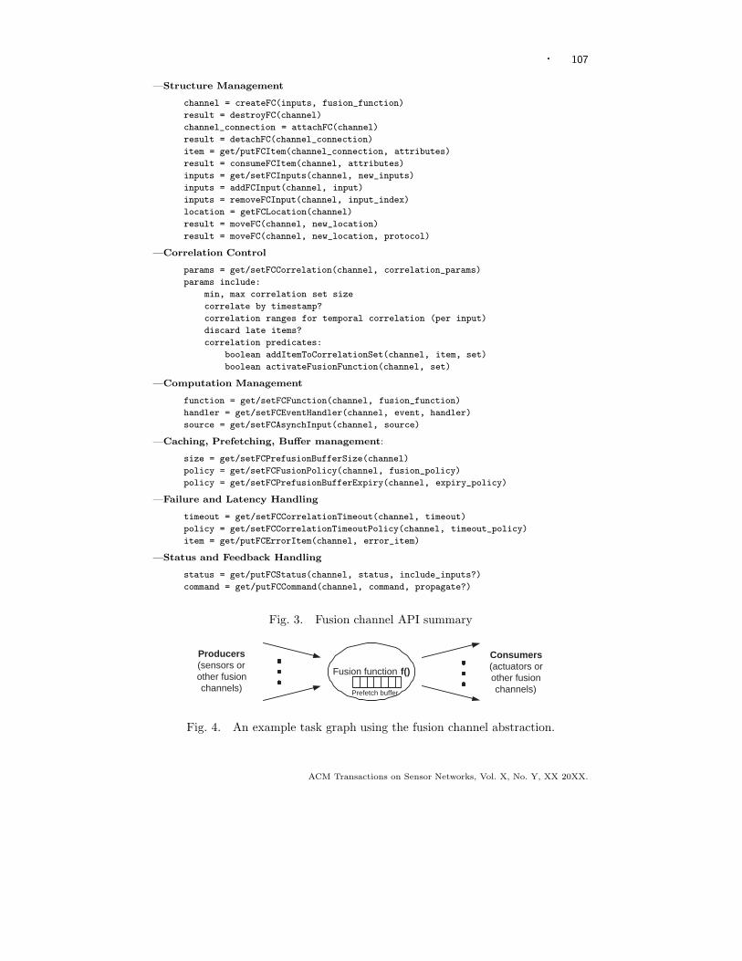
The fusion API provides capabilities that fall within the following general cate-gories:

3.1 Structure management

This category of capabilities primarily handles “plumbing” issues. The fundamentalabstraction in DFuse is the fusion channel, shown in Figure 4. It is a named,global entity that abstracts a set of inputs and encapsulates a programmer-suppliedfusion function. Inputs to a fusion channel may come from the node that hoststhe channel or from a remote node. Item fusion is automatic and is performedaccording to a programmer-specified policy either on request (demand-driven, lazy,pull model) or when input data is available (data-driven, eager, push model). Itemsare fused and accessed by timestamp (usually the capture time of the incomingdata items). An application can request an item with a particular timestampor by supplying some wildcard specifiers supported by the API (such as earliestitem, latest item). Requests can be blocking or non-blocking. To accommodatefailure and late arriving data, requests can include a minimum number of inputsrequired and a timeout interval. Fusion channels have a fixed capacity specified atcreation time. Finally, inputs to a fusion channel can themselves be fusion channels,creating fusion networks or pipelines. Using a standard or programmer-suppliedprotocol, a fusion channel may be migrated on demand to another node of thenetwork. This feature is essential for supporting the role assignment functionalityof the placement module. Upon request from an application, the state of thefusion channel is packaged and moved to the desired destination node by the fusionmodule. The fusion module handles request forwarding for channels that have beenmigrated.

3.2 Correlation control

This category of capabilities primarily handles specification and collection of “cor-relation sets” (related input items supplied to the fusion function). Fusion requiresidentification of a set of correlated input items. A simple scheme is to collect inputitems with identical application-specified sequence numbers or virtual timestamps


· 107

—Structure Management

channel = createFC(inputs, fusion_function)

result = destroyFC(channel)

channel_connection = attachFC(channel)

result = detachFC(channel_connection)

item = get/putFCItem(channel_connection, attributes)

result = consumeFCItem(channel, attributes)

inputs = get/setFCInputs(channel, new_inputs)

inputs = addFCInput(channel, input)

inputs = removeFCInput(channel, input_index)

location = getFCLocation(channel)

result = moveFC(channel, new_location)

result = moveFC(channel, new_location, protocol)

—Correlation Control

params = get/setFCCorrelation(channel, correlation_params)

params include:

min, max correlation set size

correlate by timestamp?

correlation ranges for temporal correlation (per input)

discard late items?

correlation predicates:

boolean addItemToCorrelationSet(channel, item, set)

boolean activateFusionFunction(channel, set)

—Computation Management

function = get/setFCFunction(channel, fusion_function)

handler = get/setFCEventHandler(channel, event, handler)

source = get/setFCAsynchInput(channel, source)

—Caching, Prefetching, Buffer management:

size = get/setFCPrefusionBufferSize(channel)

policy = get/setFCFusionPolicy(channel, fusion_policy)

policy = get/setFCPrefusionBufferExpiry(channel, expiry_policy)

—Failure and Latency Handling

timeout = get/setFCCorrelationTimeout(channel, timeout)

policy = get/setFCCorrelationTimeoutPolicy(channel, timeout_policy)

item = get/putFCErrorItem(channel, error_item)

—Status and Feedback Handling

status = get/putFCStatus(channel, status, include_inputs?)

command = get/putFCCommand(channel, command, propagate?)

Fig. 3. Fusion channel API summary

Fusion function f()

Prefetch buffer

Producers (sensors or other fusion channels)

Consumers (actuators or other fusion channels)

Fig. 4. An example task graph using the fusion channel abstraction.


108 ·

(which may or may not map to real-time depending on the application). Fusionfunctions may declare whether they accept a variable number of inputs and, if so,indicate bounds on the correlation set size. Correlation may involve collecting sev-eral items from each input (for example, a time-series of data items from a giveninput). Correlation may specify a given number of inputs or correlate all arrivingitems within a given time interval. Most generally, correlation can be characterizedby two programmer-supplied predicates. The first determines if an arriving itemshould be added to the correlation set. The second determines if the collection phaseshould terminate, passing the current correlation set to the programmer-suppliedfusion function.

3.3 Computation management

This category of capabilities primarily handles the specification, application, andmigration of fusion functions. The fusion function is a programmer-supplied codeblock that takes as input a set of timestamp-correlated items and produces a fuseditem (with the same timestamp) as output. A fusion function is associated withthe channel when created. It is possible to dynamically change the fusion functionafter channel creation and modify the set of inputs to a fusion channel.

3.4 Memory Management

This category of capabilities primarily handles caching, prefetching, and buffermanagement. Typically, inputs are collected and fused (on-demand) when a fuseditem is requested. For scalable performance, input items are collected (requested) inparallel. Requests on fusion pipelines or trees initiate a series of recursive requests.To enhance performance, programmers may request items to be prefetched andcached in a prefetch buffer once inputs are available. An aggressive policy prefetches(requests) inputs on-demand from input fusion channels. Buffer management dealswith sharing generated items with multiple potential consumers and determiningwhen to reclaim cached items’ space.

3.5 Failure and Latency Handling

This category of capabilities primarily allows the fusion points to perform partialfusion, i.e. fusion over an incomplete input correlation set. It deals with sensorfailure and communication latency that are common, and often indistinguishable,in sensor networks. Fusion functions capable of accepting a variable number ofinput items may specify a timeout on the interval for correlation set collection. Latearriving items may be automatically discarded or included in subsequent correlationsets. If the correlation set contains fewer items than needed by the fusion function,an error event occurs and a programmer-supplied error handler is activated. Errorhandlers and fusion functions may produce special error items as output to notifydownstream consumers of errors. Fused items include meta-data indicating theinputs used to generate an item in the case of partial fusion. Applications may usethe structure management API functions to remove the faulty input if necessary.

3.6 Status and Feedback handling

This category of capabilities primarily allows interaction between fusion functionsand data sources such as sensors that supply status information and support a


· 109

command set (for example, activating a sensor or altering its mode of operation -such devices are often a combination of a sensor and an actuator). We have observedthat application-sensor interactions tend to mirror application-device interactions inoperating systems. Sources such as sensors and intermediate fusion points reporttheir status via a “status register1.” Intermediate fusion points aggregate andreport the status of their inputs along with the status of the fusion point itself viatheir respective status registers. Fusion points may poll this register or access itsstatus. Similarly, sensors that support a command set (to alter sensor parameters orexplicitly activate and deactivate) should be controllable via a “command” register.The specific command set is, of course, device specific but the general device driveranalogy seems well-suited to control of sensor networks.

4. PLACEMENT MODULE

This module is responsible for creating an overlay of the application task graph onto the physical network that best satisfies an application-specified cost function.A network node can play one of the three roles: end point (source or sink), relay,or fusion point [Bhardwaj and Chandrakasan 2002]. In our model, the end pointsare determined by the application. The placement module embodies a distributedrole assignment algorithm that manages the overlay network, dynamically assigningfusion points to the available nodes in the network.

The role assignment algorithm has to be aware of the following properties of aWASN:

—Node Heterogeneity: Some nodes may be resource rich compared to others. Forexample, a particular node may be connected to a permanent power supply.Clearly, such nodes should be given more priority for taking on transmission-intensive roles compared to others.

—Communication Vs. Computation: Studies have shown that wireless communi-cation is more energy draining than computation in current day wireless sensornetworks [Hill et al. 2000]. It should be noted that in future wireless sensor net-works wherein we expect more significant processing in the nodes (exemplifiedby the fusion functions), computation is likely to play an increasingly importantrole in determining node energy [Wolenetz 2005].

—Dynamic Behavior: As we already mentioned (see Section 2.3), both the appli-cation and the network environment are dynamic, thus requiring role assignmentdecisions to be made fairly frequently during the lifetime of the application.Therefore, it is important that the algorithm have low overhead, and scale wellwith the size of the application and the network.

The formulation of the role assignment problem, the cost function, and the pro-posed heuristic are sensitive to the above properties. However, the experimentaland simulation results (Section 6) deal only with homogeneous network nodes.

1A register is a communication abstraction with processor register semantics. Updates overwriteexisting values, and reads always return the current status.


110 ·

4.1 The Role Assignment Problem

Given N = (Vn, En), viz.,the network topology, and T = (Vt, Et), viz.,the taskgraph, and an application specific cost metric, the goal is to find a mapping f :Vt → Vn that minimizes the overall cost. Here, Vn represents nodes of the sensornetwork and En represents communication links between them. In the task graph,Vt represents fusion functions (filter, data fusion, etc.) and Et represents flow ofdata between the fusion points. A mapping f : Vt → Vn generates an overlaynetwork of fusion points to network nodes; implicitly, this generates a mappingl : Et → {e|e ∈ En} of data flow to communication links. The focus of the roleassignment algorithm is to determine f ; determining l is the job of the routing layerand is outside the scope of this paper.

We use “fusion function” and “fusion point” interchangeably to mean the samething.

4.2 Cost Functions

We describe five sample cost functions below. They are motivated by recent researchin power-aware routing in mobile ad hoc networks [Singh et al. 1998; Jae-HwanChang and Leandros Tassiulas 2000]. The health of a node k to host a fusion roler is expressed as the cost function c(k, r). Note that the lower the value computedby the cost function, the better the node health, and therefore the better equippedthe node k is to host the fusion point r.

—Minimize transmission cost - 1 (MT1): This cost function aims to decreasethe amount of data transmission required for hosting a fusion point. Input dataneeds to be transmitted from the sources to the fusion points, and the fusionoutput needs to be propagated to the consumer nodes (possibly going throughmultiple hops). For a fusion function r with m input data sources (fan-in) and noutput data consumers (fan-out), the cumulative transmission cost for placing ron node k is formulated as:

cMT1(k, r) =

m∑

i=1

t(sourcei) ∗HopCount(inputi, k)/Rel(inputi, k)

+n

∑

j=1

t(r) ∗HopCount(k, outputj)/Rel(k, outputj)

Here, t(x) represents the amount of data transmission (in bits per unit time) of adata source x, HopCount(i, k) is the distance (in number of hops) between nodei and node k, and Rel(i, j) is a value between (0and1) representing the reliabilityof the transmission link between nodes i and j.

—Minimize power variance (MPV): This cost function aims to keep the power(energy) levels of the nodes the same. This is a simple cost function that ignoresthe actual work being done by a node and simply focuses on the remaining powerat any given node for role assignment decisions. The cost of doing any work atnode k is inversely proportional to its remaining power level power(k), and isformulated as:

cMPV (k) = 1/power(k)


· 111

—Minimize ratio of transmission cost to power (MTP): MT1 focuses onthe work done by a node. MPV focuses on the remaining power at a given node.MTP aims to give work to a node commensurate with its remaining energy level,and thus represents a combination of the first two cost functions. Intuitively, arole assignment based on MTP is a reflection of how long a given node k canhost a given fusion function r with its remaining power level power(k). Thus,the cost of placing a fusion function r on node k is formulated as:

cMTP (k, r) = cMT1(k, r) ∗ cMPV (k) = cMT1(k, r)/power(k)

—Minimize transmission cost - 2 (MT2): This cost function takes into accountnode heterogeneity. In particular, it biases the role assignment with a view toprotecting low energy nodes. It can be considered a variant of MT1, with the costfunction behaving like a step function based on the node’s remaining power level.The intuition is that if a node has wall power then its cost function is the sameas MT1. For a node that is battery powered, we would protect it from hosting(any) fusion point if its energy level goes below a predetermined threshold. Thusa role transfer should be initiated from such a node even if it results in increasedtransmission cost. This is modeled by making the cost of hosting any fusionfunction at this node infinity. This cost function is formulated as:

cMT2(k, r) = ( power(k) > threshold ) ?( cMT1(k, r) : INFINITY ))

—Minimize Computation and Communication Cost (MCC): This costfunction accounts for both the computation as well as the communication costof hosting a fusion function:

cMCC(k, r) = cMT1(k, r) ∗ eradio(k) (Communication energy)

+ cycleCount(k, r) ∗ frameRate(r) ∗ ecomp(k) (Computation energy)

This equation has two parts:(1) Communication energy: cMT1(k, r) represents the transmission cost (bits per

unit time);eradio(k) is the energy per bit consumed (Joule/bit) by the radio at node k.

(2) Computation energy: cycleCount(k,r) is the computation cost (total numberof instructions per input data item) for executing the fusion function r onnode k for a standard data input (frame) size;frameRate(r) is the number of items generated per second by r;ecomp(k) is the energy per instruction consumed (Joule/instruction) by theprocessor at node k.

If the network is homogeneous and if we assume that the processing of a givenfusion function r is data independent, then cycleCount(k, r) and ecomp(k) arethe same for any node k. In this case role assignment based on MCC behavesexactly the same as MT1.In our experimental and simulation results reported in this paper (which doesrelative comparison of our role assignment algorithm to static and optimal), we donot consider MCC any further. However, absolute network lifetime will diminishif the node energy for computation is taken into account. Such a study is outsidethe scope of this paper and is addressed in companion works [Wolenetz 2005;Wolenetz et al. 2004; 2005].


112 ·

It should be emphasized that the above cost functions are samples. The appli-cation programmer may choose to specify the health of a node using the figure ofmerit that best matches the application level requirement. The role assignmentalgorithm to be discussed shortly simply uses the application provided metric in itsassignment decisions.

4.3 In Search of Optimality

The general case of mapping an arbitrary task graph (directed) onto another ar-bitrary processor graph (undirected) is NP-complete [Garey and Johnson 1979;Papadimitriou and Yannakakis 1988]. Since DFuse treats a fusion function as ablack-box, and the application-specified cost function can be arbitrary, the generalproblem of role assignment is NP-complete.

Given specific task graphs and specific cost functions, optimal solutions can befound deterministically. For example, consider an input task graph in which allthe fusion functions are data-expanding. For transmission based cost functions(MT 1, MT 2), a trivial O(1) algorithm would place all the fusion points at thesinks (or as close as possible to the sinks if there is a problem hosting multiple rolesat a sink).��

� ��

��

��

� � � � � � � � � � � ! " # # $ % & � ' ( ) * # � % ( + , - . / � 0 � � � � � � � � � ! " # # $ % & � ' ( ) * # � % 1 2 3 � 4 . �

1 $% $! * ! 2 � $ % 5 3 5 � 1 2 3 �0 � % % 0 � $ % & 2 6 7 2 8 7 2 $ % 9� " � : � ; � 5 9 ( 5 " # < � ( = > � ? � 1 2 33 " � 9 ( 5 " # < � ( )�@ A@ B

C AC B @ D E F @ A@ B

C A @ D E F@ A@ B C B @ D E F @ A

@ BC A @ D E F

@ A@ B @ D E F C BC BC A

Fig. 5. Mapping a task graph using minimum Steiner tree (MST): Example shows that MST doesnot lead to an optimal mapping. For Gn, the edge weights can be thought of as hop counts, andfor Gt, as transmission volume. Edge weights on the overlay graphs (c and d) are obtained bymultiplying the edge weights of the task graph with those the corresponding edge weight of thenetwork links.

At the other extreme, consider a task graph where all the fusion functions are datacontracting. In this case, for transmission based cost functions, fusion functionsneed to be applied to nodes that are as close to the data sources as possible.


· 113

Therefore, finding a minimum Steiner tree (MST) of the network graph connectingthe sources and the sinks, and then mapping individual fusion functions to nodesclose to the data sources may lead to a good solution, though optimality is still notguaranteed as shown in an example mapping in Figure 5. In the example, sincean MST is obtained without considering the transmission requirements in the taskgraph, a mapping based on MST turns out to be more expensive than the optimal.Also, finding MST is APX-complete2, with best known approximation bound of1.55 [Robins and Zelikovsky 2000]. Finally, as is illustrated in this example, MSTbased solutions cannot be applied for an arbitrary task graph and cost functions.

Moreover, existing approximate solutions to Steiner tree and graph mappingproblems are impractical to be applied to sensor networks. Such solutions assumethat (1) the network topology is known, (2) costs on edges in the network areknown, and (3) the network is static. None of these assumptions hold in our case:the network topology is not known and must be discovered; costs on edges areknown locally but not globally (and it is too expensive to gather this informationat a central planner); and even if we could find the optimal deployment, because ofinherent dynamism of WASN, we need to re-deploy.

All of these considerations lead us to design a heuristic for role assignment. Thefundamental design principle is not to rely on any global knowledge.

4.4 The Role Assignment Heuristic

We have developed a heuristic that adheres to the design principle of using localinformation and not relying on any global knowledge. The heuristic goes throughthree phases: initialization, optimization, and maintenance. We describe thesethree phases in the following subsections.

4.4.1 Initialization Phase. In this phase, we make a first-cut naive assignmentof fusion points to the network nodes. The application has not started yet, andno application-specified cost function is used in this initial mapping. The onlyreal input to this phase of the algorithm is the resource constraints of the networknodes (for e.g. “is a node connected to a wall socket?”, “does a node have enoughprocessing power and memory”, etc.). The initial placement, however, has a hugeimpact on the quality of the steady-state behavior of the application. For example,if the initial mapping places a fusion point k hops away from an optimal placement,at least k role transfers are needed before reaching an optimum. Therefore, we adopteither a top-down or bottom-up approach based on the nature of the application taskgraph to make the initial placement a good starting point for the subsequent phases.Essentially, if it is known that all the fusion functions in the task graph are datacontracting, then placing them as close to the data sources as possible lowers thetransmission overhead. This is the bottom up approach, where we start from theleaves (sources) of the task graph and work towards the root (sink). On the otherhand, if the task graph has mostly data expanding fusion functions, then placingthe fusion points close to the sinks makes sense. This is the top-down approach,where the mapping starts from the root of the task graph and progresses towards

2APX is the class of optimization problems in NP, having polynomial time approximation algo-rithms


114 ·

the leaves. The default (in the absence of any a priori knowledge about the taskgraph) is to take a bottom-up approach since data contraction is more common insensor applications.

In either case, this phase is very quick. Needless to say, the mapping of sourcesand sinks to network nodes is pre-determined. Therefore, the job of the initializationphase is to determine the mapping of the fusion points to the network nodes. Inprinciple if the task graph has a depth k and the network has a depth n, an attemptis made in the initialization phase to place all the fusion points in at most k levelsof the tree either near the sources (bottom-up) or the sinks (top-down).Top-down Approach. This phase starts working from the root (sink) node3.Based on its resource constraints, the root node either decides to host the rootfusion function or not. If it decides to host the root fusion function, then it delegatesthe mapping of the children subtrees to its neighbors (either in the same level or thenext level). This role assumption and delegation of the subtrees progresses until allthe fusion functions are placed on network nodes. Relay nodes (as required) are usedto connect up the sources to the network nodes that are hosting the fusion pointsof the task graph closest to the leaves. It is possible that in this initial phase a nodemay be asked to host multiple fusion functions, and it is also possible that a nodemay decide not to host any fusion point but simply pass the incoming subtree on toone of its neighbors. In choosing delegates for the subtrees, the “resource richness”of the neighbors is taken into account. This recursive tree building ends at the datasource nodes, i.e. the leaves of the task graph. The completion notification of thetree building phase recursively bubbles up the tree from the sources to the root.Bottom-up Approach. As with the top-down approach, this phase starts at theroot node. However, the intent is to assign fusion points close to the sources dueto the data contracting nature of the task graph. To understand how this works,suppose the input task graph is a tree with depth k. The leaf nodes are the datasources. Their parents are the fusion points that are k − 1 level distant from theroot. For each fusion function at layer (k−1) the root node asks an appropriate datasource (commensurate with the task graph connectivity and avoiding duplication)to select the network nodes to host the set of fusion functions at level k−1 that areits consumers. To select the fusion node among its neighbors, the data source willprefer a node which is closer to the root node in terms of hop count. The selectednodes at level k − 1 report their identity to the root node. Once all the fusionfunctions at level (k− 1) have been thusly mapped, the root node recursively mapsthe fusion functions at the next higher levels of the tree in a similar way. As withthe top-down approach, relay nodes (as required) bridge the 1st level fusion pointsof the task graph to the root.

For the bottom-up approach, the root node plays an active role in mapping thefusion point. The alternative would be to flood the complete task graph to theleaf nodes and other participating network nodes close to the leaves. Since thedata sources can be quite far from the root such flooding can be quite expensive.Therefore, in the bottom-up approach the root node explicitly contacts a networknode that is hosting a fusion point at a given level to map its parents to network

3Note that there could be multiple root nodes (one for each sink in the application task graph).This phase of the heuristic works in parallel starting from each such root.


· 115

nodes. This was not necessary for the top-down approach, where the root nodeneeded to contact only its neighbor nodes for the mapping of the subtrees.

4.4.2 Optimization Phase. Upon completion of the initialization phase, the rootnode starts a recursive wave of “start optimization phase” message to the nodesof the network. This phase is intended to refine the initial mapping before theapplication starts. The input to this phase is the expected data flows between thefusion points and the application-specified cost function. During this phase, a nodethat is hosting a fusion point is responsible for either continuing to play that roleor transferring it to one of its neighbors. The decision for role transfer is takenby a node (that hosts that role) based on local information. With a certain pre-determined periodicity a node hosting a fusion function informs its neighbors itsrole and its health (a metric determined by the application-specified cost function).Upon receiving such a message, the recipient computes its own health for hostingthat role. If the receiving node determines that it is in better health to play thatrole, an intention to host message is sent to the sender. If the original senderreceives one or more intention messages from its neighbors, the role is transferredto the neighbor with the best health. The overall health of the overlay networkimproves with every such role transfer.

The optimization phase is time bound and is a tunable parameter of the roleassignment heuristic. Upon the expiration of the preset time bound, the root nodestarts a recursive wave of “end optimization phase” messages in the network. Eachnode is responsible in making sure that it is in a consistent state (for example, itis not in the middle of a role transfer to a neighbor) before propagating the wavedown the network. Once this message reaches the sources this phase is over, andthe application starts with data production by the sources.

4.4.3 Maintenance Phase. The maintenance phase has the same functionality asthe optimization phase. The input to this phase are the actual data flows observedbetween the fusion points and the application-specified cost function. In this phase,nodes periodically exchange role and health information and trigger role transfersif necessary. The application dynamics and/or the network dynamics leads to suchrole transfers. Any such heuristic that relies entirely on local information is proneto getting caught in local minima (see Section 4.5). To reduce such occurrences,the maintenance phase periodically increases the size of the set of neighbors anode interacts with for potential role transfer opportunities. The overhead of themaintenance phase depends on the periodicity with which the neighborhood sizeis increased and the broadcast radius of the neighborhood. These two factors areexposed as tunable parameters to the application.

4.4.4 Support for Node Failure and Recovery. Failures can occur at any of thenodes of the sensor network: sources, sinks or fusion points. A sink failure is directlyfelt by the application and it is up to the semantics of the application whether itcan continue despite such a failure. A source or intermediate fusion point failureis much more subtle. Such a failure affects the execution of the fusion functionshosted by the nodes downstream from the failed node that are expecting input fromit. The manifestation of the original node failure is the unsuccessful execution ofthe fusion functions at these downstream nodes. As we mentioned in Section 3.5,


116 ·

the fusion module has APIs to report fusion function failure to the application.The placement and fusion modules together allow recovery of the application fromfailure as detailed below.

After the first two phases of the role assignment heuristic, any node that is hostinga fusion point knows only the nodes that are consuming data from it. That is, anygiven node does not know the identity of the network nodes that are producing datafor that node. In fact, due to the localized nature of the role transfer decisions, nosingle node in the network has complete knowledge of the physical deployment ofthe task graph nor even the complete task graph. This poses a challenge in termsof recovering from failure. Fortunately, the root node has full knowledge of thetask graph that has been deployed. We describe how this knowledge is exploited indealing with node failure and recovery.

Basically, the root node plays the role of an arbiter to help resurrect a failedfusion point. Note that any data and state of the application that is lost at thefailed node has to be reconstructed by the application. The recovery procedureexplained below is to simply re-establish the complete task graph on the sensornetwork subsequent to a failure.� � � � � � � � � � � � � � � � � ��

� � � � � � � � �� Fig. 6. An example failure scenario showing a task graph overlaid on the network. An edge inthis figure may physically comprise of multiple network links. Every fusion point has only localinformation, v iz. identities of its immediate consumers.

Recovery procedure. Let the failed fusion point be at level k of the task graph,with m input producer nodes at level (k − 1) to this fusion point, and n outputconsumer nodes at level (k+1) awaiting output from this fusion point. The followingthree steps are involved in the recovery procedure:

(1) Identifying the consumers: The n consumer nodes at level (k + 1) generatefusion function failure messages (see Section 3.5). These messages along withthe IDs of the consumers are propagated through the network until they reachthe root node.

(2) Identifying the producers: Since there are m producers for the failed node,there are correspondingly m subtrees under the failed fusion function. Theroot identifies these subtrees and the data sources at the leaf of these subtrees,


· 117

respectively, by parsing the application task graph. For each of these m sub-trees, the root node selects one data source at the leaf level. The m selecteddata sources generate a probe message each (with information about the failedfusion function). These messages are propagated through the network untilthey reach the m nodes at level (k − 1). These m nodes (which are the pro-ducers of data for the failed fusion function) report their respective identitiesto the root node.

(3) Replacing the failed fusion point: At this point the root node knows the physicalidentities of the consumers and producers to the failed fusion point. It requestsone of them to choose a candidate neighbor node for hosting the failed fusionfunction. The chosen node informs the producers and consumers of the roleit has assumed and starts the fusion function. This completes the recoveryprocedure.

Needless to say, during this recovery process the consumer and producer nodes(once identified) do not attempt to do any role transfers. Also, this recovery proce-dure is not resilient to failures of the producers or the consumers (during recovery).

4.5 Analysis of the Role Assignment Heuristic

For the class of applications and the environments that the role assignment algo-rithm is targeted, the health of the overall mapping can be thought of as the sumof the health of individual nodes hosting the roles. The heuristic triggers a roletransfer only if there is a relative health improvement. Thus, it is safe to say thatsuch dynamic adaptations indeed improve the life of the network with respect tothe cost function.

The heuristic could occasionally result in the role assignment getting caught in alocal minima. However, due to the dynamic nature of WASN and the re-evaluationof the health of the nodes at regular intervals, such occurrences are short lived.For example, if ‘minimize transmission cost (MT1 or MT2)’ is chosen as the costfunction, and if the network is caught in a local minima, that would imply thatsome node is losing energy faster than an optimal node. Thus, one or more of thesuboptimal nodes die causing the algorithm to adapt the assignment. This behavioris observed in real life as well and we show it in the evaluation section.

The choice of the cost function has a direct effect on the behavior of the heuristic.We examine the behavior of the heuristic for a cost function that uses two simplemetrics: (a) simple hop-count distance, and (b) fusion data expansion or contractioninformation.��

Fig. 7. Linear Optimization


118 · � � ��

�� ! !� � " # � � � ��

� �� $% %% &' ( (� � " # � � ) � * � � � � � �

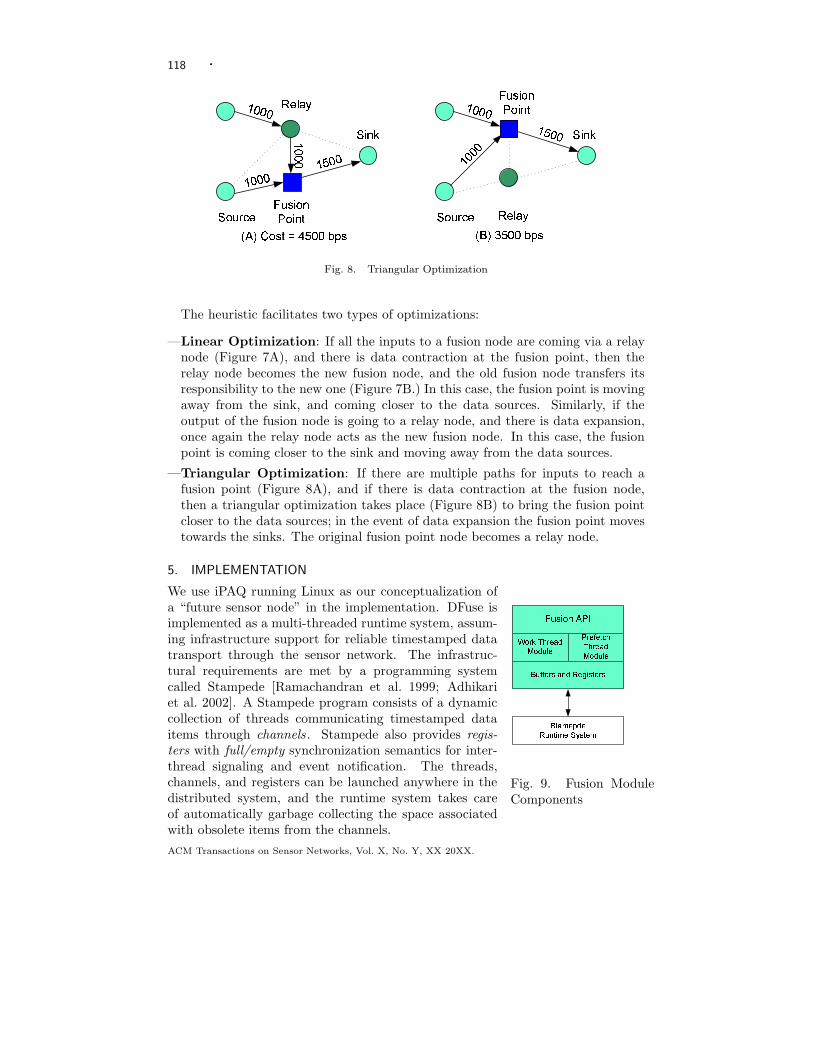
Fig. 8. Triangular Optimization

The heuristic facilitates two types of optimizations:

—Linear Optimization: If all the inputs to a fusion node are coming via a relaynode (Figure 7A), and there is data contraction at the fusion point, then therelay node becomes the new fusion node, and the old fusion node transfers itsresponsibility to the new one (Figure 7B.) In this case, the fusion point is movingaway from the sink, and coming closer to the data sources. Similarly, if theoutput of the fusion node is going to a relay node, and there is data expansion,once again the relay node acts as the new fusion node. In this case, the fusionpoint is coming closer to the sink and moving away from the data sources.

—Triangular Optimization: If there are multiple paths for inputs to reach afusion point (Figure 8A), and if there is data contraction at the fusion node,then a triangular optimization takes place (Figure 8B) to bring the fusion pointcloser to the data sources; in the event of data expansion the fusion point movestowards the sinks. The original fusion point node becomes a relay node.

5. IMPLEMENTATION + , - ./ 0 1 2 34 5 67 8 9 6: ; <= 5 < > ?: @ 6: A: B C 98 9 6: ; <= 5 < > ?:D > AA: 6E ; F < G : H IE B : 6EJ B; K : L< :G > F B IK : J M E B : KFig. 9. Fusion ModuleComponents

We use iPAQ running Linux as our conceptualization ofa “future sensor node” in the implementation. DFuse isimplemented as a multi-threaded runtime system, assum-ing infrastructure support for reliable timestamped datatransport through the sensor network. The infrastruc-tural requirements are met by a programming systemcalled Stampede [Ramachandran et al. 1999; Adhikariet al. 2002]. A Stampede program consists of a dynamiccollection of threads communicating timestamped dataitems through channels . Stampede also provides regis-ters with full/empty synchronization semantics for inter-thread signaling and event notification. The threads,channels, and registers can be launched anywhere in thedistributed system, and the runtime system takes careof automatically garbage collecting the space associatedwith obsolete items from the channels.


· 119

5.1 Fusion Module

The fusion module consists of the shaded components shown in Figure 9. It is im-plemented in C as a layer on top of the Stampede runtime system. All the buffers(input buffers, fusion buffer, and prefetch buffer) are implemented as Stampedechannels. Since Stampede channels hold timestamped items, it is a straightforwardmapping of the fusion attribute to the timestamp associated with a channel item.The Status and Command registers of the fusion architecture are implemented us-ing the Stampede register abstraction. In addition to these Stampede channels andregisters that have a direct relationship to the elements of the fusion architecture,the implementation uses additional Stampede channels and threads. For instance,there are prefetch threads that gather items from the input buffers, fuse them, andplace them in the prefetch buffer for potential future requests. This feature allowslatency hiding but comes at the cost of potentially wasted network bandwidth andhence energy (if the fused item is never used). Although this feature can be turnedoff, we leave it on in our evaluation and ensure that no such wasteful communi-cation occurs. Similarly, there is a Stampede channel that stores requests thatare currently being processed by the fusion architecture to eliminate duplication ofwork.

The createFC call from an application thread results in the creation of all theabove Stampede abstractions in the address space where the creating thread re-sides. An application can create any number of fusion channels (modulo systemlimits) in any of the nodes of the distributed system. An attachFC call from anapplication thread results in the application thread being connected to the spec-ified fusion channel for getting fused data items. For efficient implementation ofthe getFCItem call, a pool of worker threads is created in each node of the dis-tributed system at application startup. These worker threads are used to satisfygetFCItem requests for fusion channels created at this node. Since data may haveto be fetched from a number of input buffers to satisfy the getFCItem request,one worker thread is assigned to each input buffer to increase the parallelism forfetching the data items. Once fetching is complete, the worker thread rejoins thepool of free threads. The worker thread to fetch the last of the requisite inputitems invokes the fusion function and puts the resulting fused item in the fusionbuffer. This implementation is performance-conscious in two ways: first, there isno duplication of fusion work for the same fused item from multiple requesters;second, fusion work itself is parallelized at each node through the worker threads.

The duration to wait on an input buffer for a data item to be available is specifiedvia a policy flag to the getFCItem. For example, if try for time delta policy isspecified, then the worker thread will wait for time delta on the input buffer. Onthe other hand, if block policy is specified, the worker thread will wait on the inputbuffer until the data item is available. The implementation also supports partialfusion in case some of the worker threads return with an error code during fetch ofan item. Taking care of failures through partial fusion is a very crucial componentof the module since failures and delays can be common in WASN.

As we mentioned earlier, Stampede does automatic reclamation of storage spaceof data items in channels. Stampede garbage collection uses a global lower boundfor timestamp values of interest to any of the application threads (which is derived


120 ·

from a per-thread state variable called thread virtual time). Our fusion architectureimplementation leverages this feature for cleaning up the storage space in its internaldata structures (which are built using Stampede abstractions).

5.2 Placement Module

Stampede’s runtime system sits on top of a reliable UDP layer in Linux. Therefore,there is no support for adaptive multi-hop ad hoc routing in the current implemen-tation. Further, there is no support for gathering real health information of thenodes. For the purposes of evaluation, we have adopted a novel combined imple-mentation/simulation approach. The fusion module is a real implementation ona farm of iPAQs as detailed in the previous subsection. The placement moduleis an event-driven simulation of the three phases of the role assignment algorithmdescribed in Section 4. It takes an application task graph and the network topologyinformation as inputs, and generates an overlay network, wherein each node in theoverlay is assigned a unique role of performing a fusion operation. It models thehealth of the sensor network nodes. It currently assumes an ideal routing layer(every node knows a route to every other node) and an ideal MAC layer (no con-tention). Further, path reliability for MT1 and MT2 cost function evaluation isassumed to be 1 in the simulation. However, it should be clear that these assump-tions are not inherent in the DFuse architecture; they are made only to simplifythe simulator implementation and evaluation.

We have implemented an interface between the the fusion module implementationand the placement module simulation. This interface facilitates (a) collecting theactual data rates of the sensor nodes experienced by the application running onthe implementation and reporting them to the placement module simulation, and(b) communicating to the fusion module (and effecting through the DFuse APIs)dynamic task graph instantiation, role changes based on the health of the nodes,and fusion channel migration.

6. EVALUATION

We have performed an evaluation of the fusion and placement modules of the DFusearchitecture at two different levels: micro-benchmarks to quantify the overheadof the primitive operations of the fusion API including channel creation, attach-ments/detachments, migration, and I/O; and ability of the placement module tooptimize the network given a cost function. The experimental setup uses a set ofwireless iPAQ 3870s running Linux “familiar” distribution version 0.6.1 togetherwith a prototype implementation of the fusion module discussed in section 5.1.

We first describe the micro-benchmarks and then the results with the placementmodule, both for a small network of twelve iPAQs. Next, we will describe thesimulation results for a network of more than a thousand nodes, where we will onlylook at different aspects of the placement algorithm.

6.1 Micro Measurements of Fusion API

Figure 10 shows the cost of the DFuse API. In part (a), each API cost has 3 fields- local, ideal, and API overhead. Local cost indicates the latency of operation ex-ecution without any network transmission involved, ideal cost includes messaginglatency only, and API overhead is the subtraction of local and ideal costs from


· 121

0 20 40 60 80 100 120

consumeFCItem

getFCItem(1K) - 0 1 2

getFCItem(10) - 0 1 2







putFCItem(1K)

putFCItem(10)

detachFC

attachFC

destroyFC

createFC

Time (ms)

LocalIdeal (Messaging Latency Only)API Overhead for Remote

Number in () = Item Size

# # # - Configuration of Different Input, Fusion Channel, and Consumer locations (example) 0 1 1 - InpAS:0, ChanAS:1, ConsAS:1

0

100

200

300

400

500

600

0 1 2 3 4 5 6 7 8 9 10

Number of Items in Fusion Channel (Each item size = 1024 Bytes)

Cos

t (m

s)

API Overhead

Ideal Cost(Messaging Latency Only)

R2R

R2L

L2R

L2R - Local to Remote moveFCR2L - Remote to Local moveFCR2R - Remote to Remote moveFC

(a) (b)

Fig. 10. (a) Fusion Channel APIs’ cost (b) Fusion channel migration (moveFC)cost

Round Msg overhead Round Msg overheadAPI Trips (bytes) API Trips (bytes)

createFC 3 596 getFCItem(1K) - 0 1 0 6 3112destroyFC 5 760 getFCItem(10) - 0 0 1 10 1738attachFC 3 444 getFCItem(1K) - 0 0 1 10 4780detachFC 3 462 getFCItem(10) - 0 1 2 10 1738

putFCItem(10) 1 202 getFCItem(1K) - 0 1 2 10 4780putFCItem(1K) 1 1216 consumeFCItem 2 328

getFCItem(10) - 0 1 1 4 662 moveFC(L2R) 20 4600getFCItem(1K) - 0 1 1 4 1676 moveFC(R2L) 25 5360getFCItem(10) - 0 1 0 6 1084 moveFC(R2R) 25 5360

Table I. Number of round trips and message overhead of DFuse. See Figure 10 forgetFCItem and moveFC configuration legends.

actual cost on the iPAQ farm. Ideally, the remote call is the sum of messaginglatency and local cost. Fusion channels can be located anywhere in the sensor net-work. Depending on the location of the fusion channel’s input(s), fusion channel,and consumer(s), the minimum cost varies because it can involve network commu-nications. getFCItem is the most complex case, having four different configurationsand costs independent of the item sizes being retrieved. For part (a), we create fu-sion channels with capacity of ten items and one primitive Stampede channel asinput. Reported latencies are the averages of 1000 iterations.

On our iPAQ farm, netperf [Netperf 2003] indicates a minimum UDP roundtriplatency of 4.7ms, and from 2-2.5Mbps maximum unidirectional streaming TCPbandwidth. Table I depicts how many round trips are required and how many bytesof overhead exist for DFuse operations on remote nodes. From these measurements,we show messaging latency values in Figure 10(a) for ideal case costs on the farm.We calculate these ideal costs by adding latency per round trip and the cost of thetransmission of total bytes, presuming 2Mbps throughput. Comparing these idealcosts in Figure 10(a) with the actual total cost illustrates reasonable overhead forour DFuse API implementation. The maximum cost of operations on a local nodeis 5.3ms. For operations on remote nodes, API overhead is less than 74.5% of the


122 ·

ideal cost. For operations with more than 20ms observed latency, API overheadis less than 53.8% of the ideal cost. This figure also illustrates that messagingconstitutes the majority of observed latency of API operations on remote nodes.Note that ideal costs do not include additional computation and synchronizationlatencies incurred during message handling.

The placement module may cause a fusion point to migrate across nodes in thesensor fusion network. Migration latency depends upon many factors: the numberof inputs and consumers attached to the fusion point, the relative locations ofthe node where moveFC is invoked to the current and resulting fusion channel,and amount of data to be moved. Our analysis in Figure 10(b) assumes a singleprimitive stampede channel input to the migrating fusion channel, with only a singleconsumer. Part (b) shares the same ideal cost calculation methodology as part (a).Our observations show that migration cost increases with number of input itemsand that migration from a remote to a remote node is more costly than local toremote or remote to local migration for a fixed number of items. Reported latenciesare averages over 300 iterations for part (b).

(A) MT1: Minimize Transmission Cost - 1

0

500

1000

1500

2000

2500

3000

3500

4.2E

+02

1.2E

+03

1.0E

+05

4.5E

+05

8.0E

+05

1.2E

+06

1.5E

+06

1.9E

+06

2.2E

+06

2.6E

+06

2.9E

+06

3.3E

+06

3.6E

+06

4.0E

+06

Time (ms)

Net

wor

k Tr

affic

(B

ytes

/Sec

ond) Actual Placement Best Placement

(B) MPV: Minimize Power Variance

0

500

1000

1500

2000

2500

3000

3500

4.2E

+02

1.2E

+03

1.0E

+05

4.5E

+05

8.0E

+05

1.2E

+06

1.5E

+06

1.9E

+06

2.2E

+06

2.6E

+06

2.9E

+06

3.3E

+06

3.6E

+06

4.0E

+06

Time (ms)

Net

wor

k Tr

affic

(B

ytes

/Sec

ond)

(C) MTP: Ratio of Transmission Cost to Available Power

0

500

1000

1500

2000

2500

3000

3500

4.2E

+02

1.2E

+03

1.0E

+05

4.5E

+05

8.0E

+05

1.2E

+06

1.5E

+06

1.9E

+06

2.2E

+06

2.6E

+06

2.9E

+06

3.3E

+06

3.6E

+06

4.0E

+06

Time (ms)

Net

wor

k Tr

affic

(B

ytes

/Sec

ond)

(D) MT2: Minimize Transmission Cost - 2

0

500

1000

1500

2000

2500

3000

3500

4.2E

+02

1.2E

+03

1.0E

+05

4.5E

+05

8.0E

+05

1.2E

+06

1.5E

+06

1.9E

+06

2.2E

+06

2.6E

+06

2.9E

+06

3.3E

+06

3.6E

+06

4.0E

+06

Time (ms)

Net

wor

k Tr

affic

(B

ytes

/Sec

ond)

Actual Placement Best Placement Actual Placement Best Placement

Actual Placement Best Placement

Fig. 11. The network traffic timeline for different cost functions. X axis shows theapplication runtime and Y axis shows the total amount of data transmission perunit time.


· 123

6.2 Application Level Measurements of DFuse

0 Sink

1

2 5

4

3

8

7

6

11 Src

10 Src

9 Src

Fig. 12. iPAQ Farm Experiment Setup. An arrow represents that two iPAQs are mutuallyreachable in one hop.

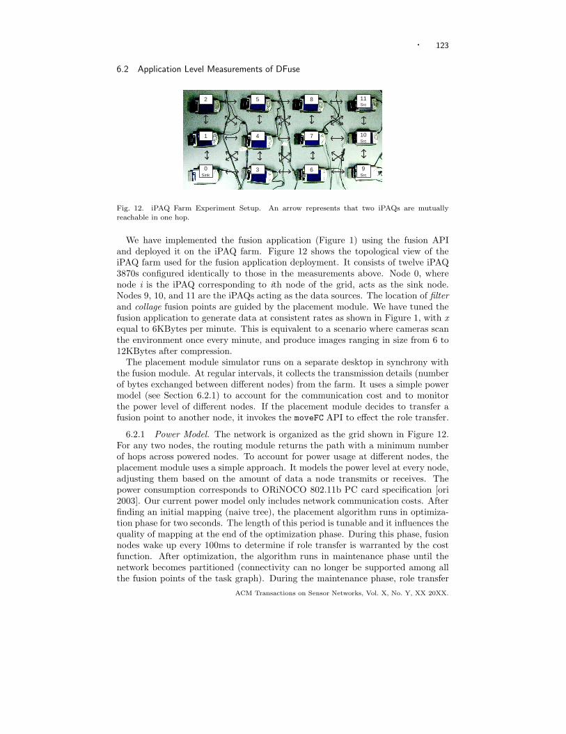
We have implemented the fusion application (Figure 1) using the fusion APIand deployed it on the iPAQ farm. Figure 12 shows the topological view of theiPAQ farm used for the fusion application deployment. It consists of twelve iPAQ3870s configured identically to those in the measurements above. Node 0, wherenode i is the iPAQ corresponding to ith node of the grid, acts as the sink node.Nodes 9, 10, and 11 are the iPAQs acting as the data sources. The location of filterand collage fusion points are guided by the placement module. We have tuned thefusion application to generate data at consistent rates as shown in Figure 1, with xequal to 6KBytes per minute. This is equivalent to a scenario where cameras scanthe environment once every minute, and produce images ranging in size from 6 to12KBytes after compression.

The placement module simulator runs on a separate desktop in synchrony withthe fusion module. At regular intervals, it collects the transmission details (numberof bytes exchanged between different nodes) from the farm. It uses a simple powermodel (see Section 6.2.1) to account for the communication cost and to monitorthe power level of different nodes. If the placement module decides to transfer afusion point to another node, it invokes the moveFC API to effect the role transfer.

6.2.1 Power Model. The network is organized as the grid shown in Figure 12.For any two nodes, the routing module returns the path with a minimum numberof hops across powered nodes. To account for power usage at different nodes, theplacement module uses a simple approach. It models the power level at every node,adjusting them based on the amount of data a node transmits or receives. Thepower consumption corresponds to ORiNOCO 802.11b PC card specification [ori2003]. Our current power model only includes network communication costs. Afterfinding an initial mapping (naive tree), the placement algorithm runs in optimiza-tion phase for two seconds. The length of this period is tunable and it influences thequality of mapping at the end of the optimization phase. During this phase, fusionnodes wake up every 100ms to determine if role transfer is warranted by the costfunction. After optimization, the algorithm runs in maintenance phase until thenetwork becomes partitioned (connectivity can no longer be supported among allthe fusion points of the task graph). During the maintenance phase, role transfer


124 ·

0 10 20 30

40 50 60

70 80

90 100

Run Time

(normalized)

Remaining

Capacity (%)

Number of Role

Transfers

(absolute)

MT2

MPV

MTP

(B) (A)

0.0E+00

5.0E+05

1.0E+06

1.5E+06 2.0E+06

2.5E+06

3.0E+06

3.5E+06

4.0E+06 4.5E+06

420

1620

3E+

05

8E+

05

1E+

06

2E+

06

2E+

06

3E+

06

3E+

06

3E+

06

4E+

06

Time (ms)

Pow

er V

aria

nce

MT2

MPV

MTP

Fig. 13. Comparison of different cost functions. Application runtime is normalizedto the best case (MT2), and total remaining power is presented as the percentageof the initial power.

decisions are evaluated every 50 seconds. The role transfers are invoked only whenthe health improves by a threshold of 5%.

6.2.2 Experimental Results. Figure 11 shows the network traffic per unit time(sum of the transmission rate of every network node) for the cost functions discussedin Section 4.2. It compares the network traffic for the actual placement with respectto the best possible placement of the fusion points (best possible placement is foundby comparing the transmission cost for all possible placements). Note that theapplication runtime can be increased by simply increasing the initial power level ofthe network nodes.

In MT1, the algorithm finds a locally best placement by the end of the opti-mization phase itself. The optimized placement is only 10% worse than the bestplacement. The same placement continues to run the application until one of thefusion points (one with the highest transmission rate) dies, i.e. the remaining capac-ity becomes less than 5% of the initial capacity. If we do not allow role migration,the application will stop at this time. But allowing role migration, as in MT2, en-ables the migrating fusion point to keep utilizing the power of the available networknodes in the locally best possible way. Results show that MT2 provides maximumapplication runtime, with an 110% increase compared to that for MT1. The ob-served network traffic is at most 12% worse than the best possible for the first halfof the run, and it is the same as the best possible rate for the latter half of the run.MPV performs the worst while MTP has comparable network lifetime as MT2.Figure 11 also shows that running the optimization phase before instantiating theapplication improves the total transmission rate by 34% compared to the initialnaive placement.

Though MPV does not provide comparably good network lifetime (Figure 11B),it provides the best (least) power variance compared to other cost functions (Fig-ure 13A). Since MT1 and MT2 drain the power of fusion nodes completely beforerole migration, they show worst power variance. Also, the number of role migra-tions is minimum compared to other cost functions (Figure 13B). These resultsshow that the choice of the cost function depends on the application context and


· 125

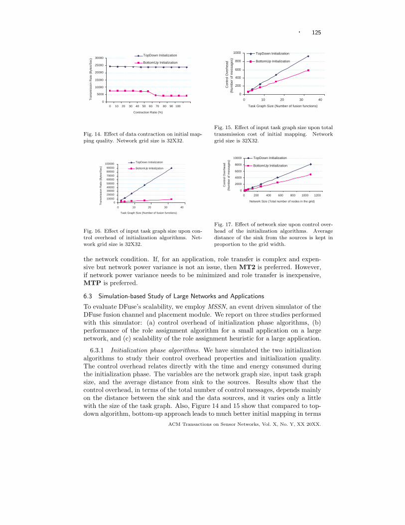
0

5000

10000

15000

20000

25000

30000

0 10 20 30 40 50 60 70 80 90 100

Contraction Ratio (%)

Tra

nsm

issi

on R

ate

(Byt

es/S

ec)

TopDown Initialization

BottomUp Initialization

Fig. 14. Effect of data contraction on initial map-ping quality. Network grid size is 32X32.

0

200

400

600

800

1000

0 10 20 30 40

Task Graph Size (Number of fusion functions)

Con

trol

Ove

rhea

d

(Num

ber

of m

essa

ges)



Fig. 15. Effect of input task graph size upon totaltransmission cost of initial mapping. Networkgrid size is 32X32.

0 10000

20000 30000 40000 50000

60000 70000

80000 90000

100000

0 10 20 30 40

Task Graph Size (Number of fusion functions)

Tra

nsm

issi

on R

atio

(B

ytes

/Sec

)



Fig. 16. Effect of input task graph size upon con-trol overhead of initialization algorithms. Net-work grid size is 32X32.

0

2000

4000

6000

8000

10000

0 200 400 600 800 1000 1200

Network Size (Total number of nodes in the grid)

Con

trol

Ove

rhea

d

(Num

ber

of m

essa

ges)



Fig. 17. Effect of network size upon control over-head of the initialization algorithms. Averagedistance of the sink from the sources is kept inproportion to the grid width.

the network condition. If, for an application, role transfer is complex and expen-sive but network power variance is not an issue, then MT2 is preferred. However,if network power variance needs to be minimized and role transfer is inexpensive,MTP is preferred.

6.3 Simulation-based Study of Large Networks and Applications

To evaluate DFuse’s scalability, we employ MSSN, an event driven simulator of theDFuse fusion channel and placement module. We report on three studies performedwith this simulator: (a) control overhead of initialization phase algorithms, (b)performance of the role assignment algorithm for a small application on a largenetwork, and (c) scalability of the role assignment heuristic for a large application.

6.3.1 Initialization phase algorithms. We have simulated the two initializationalgorithms to study their control overhead properties and initialization quality.The control overhead relates directly with the time and energy consumed duringthe initialization phase. The variables are the network graph size, input task graphsize, and the average distance from sink to the sources. Results show that thecontrol overhead, in terms of the total number of control messages, depends mainlyon the distance between the sink and the data sources, and it varies only a littlewith the size of the task graph. Also, Figure 14 and 15 show that compared to top-down algorithm, bottom-up approach leads to much better initial mapping in terms


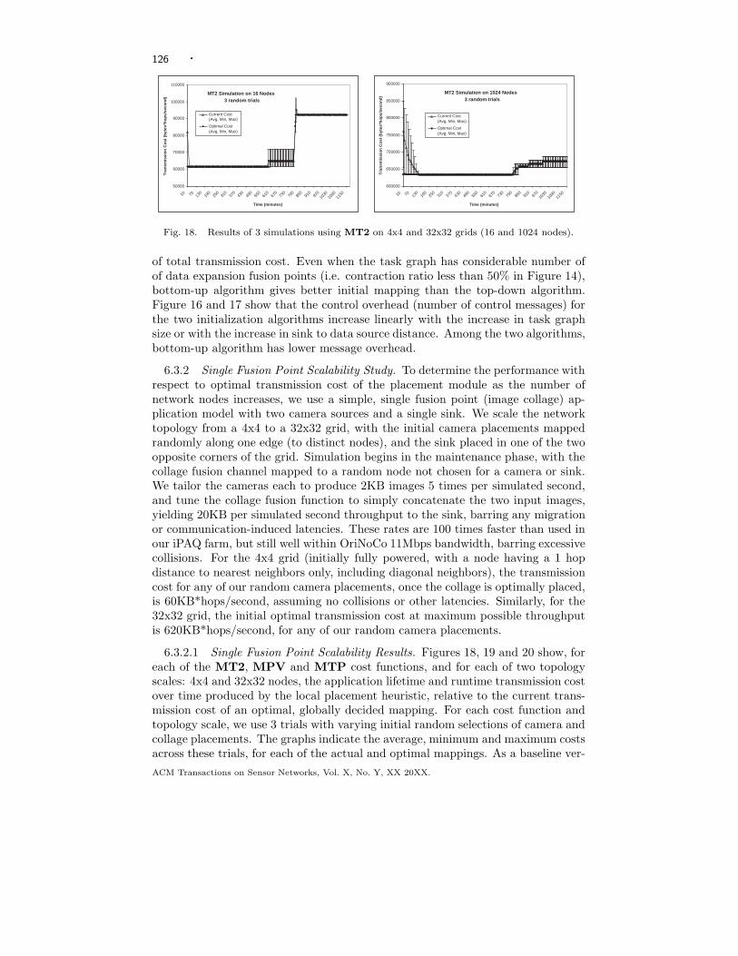
126 ·

MT2 Simulation on 16 Nodes 3 random trials

50000

60000

70000

80000

90000

100000

110000

10

70

130

190

250

310

370

430

490

550

610

670

730

790

850

910

970

1030

1090

1150

Time (minutes)

Tra

nsm

issi

on C

ost (

byte

s*ho

ps/s

econ

d)

Current Cost (Avg, Min, Max)

Optimal Cost (Avg, Min, Max)

MT2 Simulation on 1024 Nodes 3 random trials

600000

650000

700000

750000

800000

850000

900000

10

70

130

190

250

310

370

430

490

550

610

670

730

790

850

910

970

1030

1090

1150

Time (minutes)

Tra

nsm

issi

on C

ost (

byte

s*ho

ps/s

econ

d)



Fig. 18. Results of 3 simulations using MT2 on 4x4 and 32x32 grids (16 and 1024 nodes).

of total transmission cost. Even when the task graph has considerable number ofof data expansion fusion points (i.e. contraction ratio less than 50% in Figure 14),bottom-up algorithm gives better initial mapping than the top-down algorithm.Figure 16 and 17 show that the control overhead (number of control messages) forthe two initialization algorithms increase linearly with the increase in task graphsize or with the increase in sink to data source distance. Among the two algorithms,bottom-up algorithm has lower message overhead.

6.3.2 Single Fusion Point Scalability Study. To determine the performance withrespect to optimal transmission cost of the placement module as the number ofnetwork nodes increases, we use a simple, single fusion point (image collage) ap-plication model with two camera sources and a single sink. We scale the networktopology from a 4x4 to a 32x32 grid, with the initial camera placements mappedrandomly along one edge (to distinct nodes), and the sink placed in one of the twoopposite corners of the grid. Simulation begins in the maintenance phase, with thecollage fusion channel mapped to a random node not chosen for a camera or sink.We tailor the cameras each to produce 2KB images 5 times per simulated second,and tune the collage fusion function to simply concatenate the two input images,yielding 20KB per simulated second throughput to the sink, barring any migrationor communication-induced latencies. These rates are 100 times faster than used inour iPAQ farm, but still well within OriNoCo 11Mbps bandwidth, barring excessivecollisions. For the 4x4 grid (initially fully powered, with a node having a 1 hopdistance to nearest neighbors only, including diagonal neighbors), the transmissioncost for any of our random camera placements, once the collage is optimally placed,is 60KB*hops/second, assuming no collisions or other latencies. Similarly, for the32x32 grid, the initial optimal transmission cost at maximum possible throughputis 620KB*hops/second, for any of our random camera placements.

6.3.2.1 Single Fusion Point Scalability Results. Figures 18, 19 and 20 show, foreach of the MT2, MPV and MTP cost functions, and for each of two topologyscales: 4x4 and 32x32 nodes, the application lifetime and runtime transmission costover time produced by the local placement heuristic, relative to the current trans-mission cost of an optimal, globally decided mapping. For each cost function andtopology scale, we use 3 trials with varying initial random selections of camera andcollage placements. The graphs indicate the average, minimum and maximum costsacross these trials, for each of the actual and optimal mappings. As a baseline ver-


· 127

MPV Simulation on 16 Nodes 3 random trials

50000

70000

90000

110000

130000

150000

170000

190000

210000

230000

250000

10 70 130 190 250 310 370 430 490 550 610 670 730 790

Time (minutes)

Tra

nsm

issi

on C

ost (

byte

s*ho

ps/s

econ

d) Current Cost

(Avg, Min, Max)


MPV Simulation on 1024 Nodes 3 random trials

600000

700000

800000

900000

1000000

1100000

1200000

1300000

1400000

10

70

130

190

250

310

370

430

490

550

610

670

730

790

850

910

970

1030

1090

1150

Time (minutes)

Tra

nsm

issi

on C

ost (

byte

s*ho

ps/s

econ

d)



Fig. 19. Results of 3 simulations using MPV on 4x4 and 32x32 grids (16 and 1024 nodes).

MTP Simulation on 16 Nodes 3 random trials

0

50000

100000

150000

200000

250000

10 70 130 190 250 310 370 430 490 550 610 670 730 790 850 910 970

Time (minutes)

Tra

nsm

issi

on C

ost (

byte

s*ho

ps/s

econ

d)



MTP Simulation on 1024 Nodes 3 random trials

600000

650000

700000

750000

800000

850000

900000

10

70

130

190

250

310

370

430

490

550

610

670

730

790

850

910

970

1030

1090

1150

Time (minutes) T

rans

mis

sion

Cos

t (by

tes*

hops

/sec

ond)



Fig. 20. Results of 3 simulations using MTP on 4x4 and 32x32 grids (16 and 1024 nodes).

MT2 Simulations

0 100 200 300 400

0

1

2

3

4

5

6

7

8

9

10

11

12

13

14

15

16

H o

p s f r

o m o

p t i m

a l (

M T

2 ) p

l a c e

m e n

t

MPV Simulations

0 100 200 300

0

1

2

3

4

5

6

7

8

9

10

11

12

13

14

15

16

MTP Simulations

0 100 200

0

1

2

3

4

5

6

7

8

9

10

11

12

13

14

15

16

Number of placement decisions resulting in this distance from ‘optimal’

1024 Nodes

16 Nodes

Fig. 21. Proximity to optimal (transmission cost) mapping in terms of number of hops an in-stant migration would need to take from current mapping, evaluated at every placement heuristicexecution.

ification, the initial optimal transmission costs depicted in these figures agree withthe predicted 60KB*hops/second for the 4x4 topology and 620KB*hops/second forthe 32x32 topology. Furthermore, as nodes die, even the optimal costs increase asredundant, but more expensive resources are leveraged by the placement heuristic.

For MT2 (Figure 18), actual placement corresponds closely to the optimal place-ments for the 4x4 topology, and rapidly converges to optimal mapping followed byslow degradation for 32x32 topology. For MPV (Figure 19), transmission cost forthe majority of network lifetime is approximately 50-100% more than an optimalmapping. Minimizing power variance leads to frequent migrations and transmis-


128 ·

sion cost-agnostic behavior, hence the high variance in transmission cost over thelife of the network. For MTP (Figure 20), actual placement rapidly converges toan optimal mapping, followed by moderate degradation and increasing variance astransmission cost is traded off for greater mapping stability as battery variancesincrease. The performance rankings of each of these cost functions remain the sameas the network scale increases from the iPAQ-farm to the 1024 node simulation:MT2 achieves very close to optimal transmission cost, even in the 32x32 node sim-ulation, followed by MTP and then MPV. MT2 and MTP consistently achievethe greatest application lifetime, although MPV achieves the same lifetime in onecase: When the simple application is simulated on a large, 32x32 sensor networktopology, the lifetime of the network is limited by the energy in “hot spot” criticalnodes adjacent to the sink. Even though costly migrations and high-transmissioncost mappings result from using MPV, there are enough redundant resources inthe network to let the application survive until the sink’s neighbors die.

Figure 21 gives overall summaries of the proximity of the locally decided col-lage placement to the globally optimal transmission cost placement, for each of thecost functions and network scales studied. 0 hops dominate for MT2 because itperforms close to optimal. This figure also indicates that examining neighbors fur-ther away than 1 hop during placement decisions may not be necessary for MT2,as an optimal mapping is never further than a single hop away from the currentmapping in our experiments. MPV usage results in poor (large) numbers of hopsto get to the best transmission cost mapping because MPV does not attempt tooptimize transmission cost. Although a multihop placement heuristic may assistin minimizing battery variance for large networks, it makes no practical sense todo this because the transmission cost will remain unoptimized for MPV while themigration cost would increase, further reducing lifetime performance for MPV. Inessence, battery variance might be minimized, but no real work beyond migrationwould be done. MTP has generally close proximity to the best transmission costmapping, closer than MPV but not as close as MT2. As this cost-function par-tially optimizes for transmission cost, a multihop placement heuristic may assistin reducing transmission cost and increasing application lifetime. However, in thenext section we show that MT2, MTP and MPV perform well in terms of costrelative to our best “optimal” cost as scale increases, countering the need for amultihop placement heuristic.

6.3.3 Large Application Scalability Study. We extend MSSN to include threegeneral-purpose oracles to determine “optimal”4 cost in the context of MT2, MPVor MTP cost function. For small applications, we implement a general brute forceoracle, BF, that evaluates all nf possible mappings. We also employ two differenttunings, SA1 and SA2 of a simulated annealing algorithm in the form of twoapproximating oracles.

4Applications with f fusion points mappable to n sensor nodes have nf possible mappings, makingdetermination of optimality for realistic applications having more than 10 fusion points imprac-tical, especially as the application scale increases. We approach the problem of determiningoptimality by using approximation algorithms with feasible complexity.


· 129

Algorithm 6.1: SA-Oracle(type, channels, nodes, costFunction(), Tcold)

for each c ∈ channelsdo c.host← random node ∈ nodes

currentCost←∑

c∈channels costFunction(c)T ← (−average(∆cost for each neighbor with higher cost)/ln(0.80))if type = SA1then iterationsPerT emperature← |channels|2

else iterationsPerT emperature← |channels| ∗ |nodes|//SA2temperatureCount← 0repeatoldCost← currentCostfor i← 1 to iterationsPerT emperature

do

candidate← random neighbor of current stateif (∆cost(current to candidate) < 0)

then current state← candidate//Accept

else if random number ∈ [0, 1] < exp(−∆cost/T )then current state← candidate//Accept

else //RejectT ← T ∗ 0.95temperatureCount← temperatureCount + 1

until (type = SA1 and(T < Tcold or temperatureCount > |nodes|2 or currentCost = oldCost))or (type = SA2 and T < Tcold)

In our SA1 and SA2 oracles, the state of our system is described by the currentmapping of fusion channels onto nodes, where a node may host multiple fusion chan-nels simultaneously. The oracles take the application-specified DFuse cost functionsummed over all f fusion channels as the objective function. We use two basic typesof randomized permutations to reach a neighbor state: picking a new host at ran-dom for a fusion channel chosen at random, or swapping the hosts of two randomlychosen fusion channels. We choose a sufficiently high initial temperature in theunits of the global cost function by solving for T, given an input parameter for theprobability of accepting an average cost increase initially (80%), and by averagingany cost increases across all neighbors of the initial state. Each successive temper-ature is a fraction (95%) of the previous temperature. SA1 and SA2 differ in thenumber of perturbations considered at each temperature level, and in the definitionof the frozen state. SA1 is tuned to perform a significantly smaller search thanSA2 for large state spaces. SA1 evaluates f2 perturbations at each temperaturelevel and terminates annealing when T < Tcold, the number of temperature reduc-tions has exceeded n2 or when the cost at the end of a temperature level is the sameas at the beginning. SA2 evaluates f ∗ n perturbations at each temperature leveland terminates annealing only when T < Tcold. By empirically observing whenSA2 costs do not change as T decreases for more than 4 successive temperaturelevels, we define Tcold for each of the DFuse cost functions. Pseudocode for our


130 ·

Fusion Footprint (kb)Function Description Input Output Runtime

Collage Combines two inputs into one output 56*2 112 0Select Selects one of two inputs 56*2 56 0

EdgeDetect Annotates one input 56 56 0MotionDetect Compares one input to previous 56 56 94

Table II. Scalable Application Model: Fusion Functions

Camera

Camera

Motion Detect

Edge Detect

Collage

Sink

Idle Node Source/Sink

Relay

Legend

Fusion Ch.

Fig. 22. Scalable Application Model: Sample 3 Fusion Point Application on 16x16Grid

SA1 and SA2 oracles is in Algorithm 6.1.For this large application scalability study, we construct a scalable application

workload model based on workloads used in previous MSSN studies [Wolenetz et al.2004]. The task graph consists of a tree composed from subgraphs comprised offusion channels that combine 2 inputs into 1 output stream and fusion channelsthat transform 1 input into 1 output stream. We only consider the time and energyused to transmit inputs, outputs and channel buffer and state migration when de-termining resource consumption. Table II shows these data sizes for each function.For example, the Select function takes two 56kb inputs and outputs 56kb each iter-ation, and the MotionDetect channel migrates 94kb in addition to any buffer state.We configure the sensor network to be a 256 node 16x16 grid with rectilinear and


· 131

0.4 0.6 0.8

1 1.2 1.4 1.6 1.8

2 2.2 2.4 2.6

<45,16><21,8><9,4><3,2>Rat

io o

f DF

use

Cos

t to

Ora

cle

Cos

tµ,

±σ,

10

tria

ls

Application Scale <fusion points,cameras>

Cost Ratios at Varying Application Scales16x16 Nodes, Cost Function=MT2

DFuse/SA1DFuse/SA2

DFuse/Optimal

1e-06

1e-05

1e-04

0.001

0.01

0.1

1

<45,16><21,8><9,4><3,2>

Rat

io o

f DF

use

to O

racl

eM

appi

ngs

Sea

rche

d (µ

, ±σ,

10

tria

ls)


Complexity Ratios at Varying Application Scales16x16 Nodes, Cost Function=MT2

DFuse/SA1DFuse/SA2

DFuse/Optimal

Fig. 23. Large Application Scalability Results For MT2

1

1.2

1.4

1.6

1.8

2

2.2

2.4

2.6

<45,16><21,8><9,4><3,2>Rat

io o

f DF

use

Cos

t to

Ora

cle

Cos

tµ,

±σ,

10

tria

ls


Cost Ratios at Varying Application Scales16x16 Nodes, Cost Function=MTP

DFuse/SA1DFuse/SA2

DFuse/Optimal

1e-06

1e-05

1e-04

0.001

0.01

0.1

<45,16><21,8><9,4><3,2>R

atio

of D

Fus

e to

Ora

cle

Map

ping

s S

earc

hed

(µ, ±

σ, 1

0 tr

ials

)Application Scale <fusion points,cameras>

Complexity Ratios at Varying Application Scales16x16 Nodes, Cost Function=MTP

DFuse/SA1DFuse/SA2

DFuse/Optimal

Fig. 24. Large Application Scalability Results For MTP

0.9

1

1.1

1.2

1.3

1.4

1.5

1.6

1.7

1.8

<45,16><21,8><9,4><3,2>Rat

io o

f DF

use

Cos

t to

Ora

cle

Cos

tµ,

±σ,

10

tria

ls


Cost Ratios at Varying Application Scales16x16 Nodes, Cost Function=MPV

DFuse/SA1DFuse/SA2

DFuse/Optimal

1e-06

1e-05

1e-04

0.001

0.01

0.1

<45,16><21,8><9,4><3,2>

Rat

io o

f DF

use

to O

racl

eM

appi

ngs

Sea

rche

d (µ

, ±σ,

10

tria

ls)


Complexity Ratios at Varying Application Scales16x16 Nodes, Cost Function=MPV

DFuse/SA1DFuse/SA2

DFuse/Optimal

Fig. 25. Large Application Scalability Results For MPV

diagonal nearest-neighbor connectivity and initially map the application onto it ina form much like a tree. The number of fusion points is determined by the numberof camera sources used, thereby easily scaling the application. Figure 22 presentsa sample 2 camera, 3 fusion point application’s initial mapping (on a much smallergrid here). Larger application scales are formed by combining subgraphs like thesetogether into a larger tree.

6.3.3.1 Large Application Scalability Results. Figures 23, 24 and 25 show, foreach of the MT2, MTP and MPV cost functions, and for several larger scaleapplications, the performance and runtime complexity of the DFuse local placementheuristic relative to BF, SA1 and SA2 oracles. For each cost function, oracle and


132 ·

application scale, we perform 10 trials using different random seeds for the simulatedannealing oracles and for the random choice among similar arity fusion functionswhen generating the application task graphs. The graphs indicate the average and+/- one standard deviation across trials. For example, Figure 24 shows that DFuseachieves an average cost 2.2 times higher than SA2 for MTP with a 9 camera,4 fusion point application, but only searches about 1/10,000 of the mappings thatSA2 searches. It is computationally infeasible to run BF for large applicationscales, but we include it for the 3 fusion point, 2 camera configuration as an optimalbaseline.

For MT2, Figure 23 shows that DFuse outperforms SA1 at all application scalesstudied. This is likely due to the relatively small portion of the state space thatcontains globally minimum transmission cost mappings. SA1 searches f2 map-pings per temperature, and can terminate temperature reductions much soonerthan SA2, resulting in searching a very small portion of the search space (about1/100,000 for the smallest application scale studied). SA2 performs optimally atthis small application scale. For MT2, DFuse performs about the same relativeto SA1 and SA2 as scale increases. While it is impractical to implement a globalalgorithm such as SA2 in our sensor networks, we see that it would perform onlyabout twice as good as DFuse at the cost of much larger runtime complexity.

For MTP, Figure 24 shows that DFuse approaches both SA1 and SA2 andthe standard deviation decreases as scale increases. Inspection of simulation tracesalso indicates that DFuse performs about the same amount of searching and SA2performs about twice the amount of searching for MTP vs MT2. While it isinfeasible to perform a brute force search at larger scales, it is quite interestingto see that DFuse approaches our best feasibly computed optimal global oracle atlarger scales for MTP.

For MPV, Figure 25 shows that SA1 and SA2 perform similarly as scale in-creases (similar means, similar increasing standard deviations). The existence ofsimilar means between SA1 and SA2 confirms intuition that using MPV results ina large number of global mappings close to the optimum mapping. For smaller ap-plications, many of the nodes will remain idle and therefore have equivalent MPVcosts. As application scale increases, standard deviation increases, reflecting thelarger number of battery level equivalence classes across the nodes. These resultsindicate that we could expect good MPV performance on average as applicationscale increases because SA1 and SA2 perform about 1.1 to 1.3 times as good asDFuse on average across all scales studied.

6.3.4 Placement Heuristic Results Summary. Our simulation experiments withlarger networks and applications confirm our intuitions about the scalability of therole assignment heuristic:

—As the network is scaled up to 1024 nodes for a single fusion point application,all three cost functions behave similarly with respect to each other in terms oftransmission cost relative to the current optimal transmission cost: MT2 per-forms close to optimal, followed by MTP; MPV performs the worst.

—Scalability results, in terms of application lifetime, confirm that more complexcost functions that incorporate transmission energy costs (MT2 and MTP) are


· 133

able to extend lifetimes better than MPV, and that increasing redundant energyresources (nodes) in WASN can further extend lifetimes when using the migrationfacility of DFuse.

—For large topologies and small applications studied, we find that the energy of theneighbors of the fusion application’s powered sources and sinks typically deter-mines the lifetime of the application. In this case, there are so many redundantin-network nodes that the lifetime is limited by the fixed location of applicationendpoints (sources and sinks are assumed to not migrate).

—Examining neighbors further than 1 hop away from a fusion point during a localplacement decision to achieve good transmission cost performance is unnecessaryfor MT2 and MTP, and nonsensical for MPV.

—Most importantly, DFuse’s placement heuristic performs well with respect toour best feasibly computed globally optimal performance as application scaleincreases for each of the cost functions. We show that heuristic performanceactually improves relative to this optimal for MTP as application scale increases.

7. RELATED WORK

Data fusion, or in-network aggregation, is a well-known technique in sensor net-works. Research experiments have shown that it saves considerable amount ofpower even for simple fusion functions like finding min, max or average reading ofsensors [Madden et al. 2002; Intanagonwiwat et al. 2000]. While these experimentsand others have motivated the need for a good role assignment approach, they donot use a dynamic heuristic for the role assignment and their static role assignmentapproach is not amenable to streaming media applications.

Using a dataflow (task) graph to model distributed applications is a common tech-nique in streaming databases, computer vision, and robotics [Cherniack et al. 2003;Viola and Jones 2001; Rehg et al. 1997]. DFuse employs a script based interfaceto express task graph applications over the network similar to SensorWare [Bouliset al. 2003]. SensorWare is a framework for programming sensor networks, but itsfeatures are orthogonal to what DFuse provides. Specifically, 1) SensorWare doesnot employ any strategy for assigning roles to minimize the transmission cost, ordynamically adapt the role assignment based on available resources. It leaves theonus to the applications. 2) Since DFuse focuses on providing support for fusion inthe network, the interface to write fusion-based applications using DFuse is quitesimple compared to writing such applications in SensorWare. 3) DFuse providesoptimizations like prefetching and support for buffer management which are notyet supported by other frameworks. Other approaches, like TAG [Madden et al.2002], look at a sensor network as a distributed database and provide a query-basedinterface for programming the network. TAG uses an SQL-like query language andprovides in-network aggregation support for simple classes of fusion functions. TAGassumes a static mapping of roles to the network, i.e. a routing tree is built basedon the network topology and the query on hand.

Database researchers have recently examined techniques for optimizing continu-ous queries over streaming data. In many cases, the systems are centralized, andall of the processing occurs on one machine [Chen et al. 2000; Motwani et al. 2003;Chandrasekaran et al. 2003]. The need to schedule operators over distributed,


134 ·

heterogeneous, resource constrained devices presents fundamentally different chal-lenges. More recently, researchers have examined distributed stream processing,where computations are pushed into the network much as in DFuse [Ahamad andCetintemel 2004; Pietzuch et al. 2006]. Unlike DFuse, these systems usually assumepowerful in-network computation nodes, and attempt to minimize individual met-rics like network usage and maximize throughput. For example, SBON [Pietzuchet al. 2006] employs every node to run Vivaldi algorithm and generate a latency costspace of whole network to facilitate operator placement. DFuse allows a variety ofoptimization functions so that the processing can be carried out on lower-capability,energy-constrained devices.

Moreover, a common technique in data stream systems is to reorder filter andjoin (e.g. fusion) operations, according to the rules of relational algebra, in orderto optimize network placement [Srivastava et al. 2005]. Similarly, systems such asAurora* [Cherniack et al. 2003] allow “box sliding” (e.g., moving operators) and“box splitting” (e.g., splitting computation between two copies of an operator), butassume that the semantics of the operator are known in order to determine whichreconfigurations are allowable. Our system is meant to deal with task graphs wherethe computations are complex black boxes, and where operations often cannot bereordered.

Some work has looked at in-network processing of streams using resource con-strained devices [Madden et al. 2002] but have focused primarily on data aggre-gation. Our work also addresses data fusion, which utilizes more complex com-putations on specific streams and requires novel role assignment and migrationtechniques. Java object migration in MagnetOS [Liu et al. 2005] is similar in spiritto the role migration in DFuse, but MagnetOS does not allow the application tospecify its own cost function to affect the migration behavior.

Other areas where distributed tree optimization has been looked at include dis-tributed asynchronous multicast [Bhattacharya et al. 2003], and hierarchical cachetree optimization on the Internet [Tewari et al. 1999]. However, these optimiza-tions are done only with respect to the physical network properties, and they donot need to consider any input task graph characteristics (fusion function depen-dencies, black-box treatment, etc) and sensor network requirements (dynamism,energy). One recent work in composing streaming applications over peer-to-peerenvironments [Gu and Nahrstedt 2005] has looked at an optimization problem ofour flavor, but the proposed algorithm adapts a mapping only in lieu of node fail-ures, thus it is not suitable for WASN environments that need much more dynamicadaptations.

Recent research in power-aware routing for mobile ad hoc networks [Singh et al.1998; Jae-Hwan Chang and Leandros Tassiulas 2000] proposes power-aware metricsfor determining routes in wireless ad hoc networks. We use similar metrics to for-mulate different cost functions for our DFuse placement module. While designing apower-aware routing protocol is not the focus of this paper, we are looking into howthe routing protocol information can be used to define more flexible cost functions.

8. FUTURE WORK

There are several avenues for future research.


· 135

—While the applications targeted by the DFuse architecture are general (see Sec-tion 2), the role assignment algorithm assumes knowledge of the data sources fordeploying a task graph on the sensor network. This assumption is limiting for ad-dressing data centric queries where such knowledge is not available a priori. Weare exploring different ways to handle this additional source of dynamism in taskgraph deployment. One possible approach is to have an interest-disseminationphase before the initialization phase of the role assignment algorithm. Duringthis phase, the interest set of individual nodes (for specific data) is disseminatedas is done in directed diffusion [Intanagonwiwat et al. 2000]. When the responsepackets from the sources reach the sink (root node of the application task graph),the source addresses are extracted and recorded for later use in other phases ofthe role assignment algorithm.

—We plan to study the role assignment behavior in the presence of node mobil-ity and/or failure. We expect future iterations of this algorithm to gracefullyadapt fusion point placements in the presence of mobility and failures as is donecurrently to conserve power. The cost function may need to include parameterspertaining to mobility and node failures.

—We are also investigating techniques for simultaneously deploying multiple appli-cation task graphs, including such issues as algorithms for dynamically detectingsuch overlap, quantifying the energy saving afforded by merging the overlappingsubgraphs, and techniques for merging subgraphs.

9. CONCLUSION

As the form factor of computing and communicating devices shrinks and the capa-bilities of such devices continue to grow, it has become reasonable to imagine ap-plications that require rich computing resources today becoming viable candidatesfor future sensor networks. With this futuristic assumption, we have embarked ondesigning APIs for mapping fusion applications such as distributed surveillance onwireless ad hoc sensor networks. We argue that the proposed framework will easethe development of complex fusion applications for future sensor networks. Ourframework uses a novel distributed role assignment algorithm that will increase theapplication runtime by doing power-aware, dynamic role assignment. We validateour arguments by designing a sample application using our framework and evalu-ating the application on an iPAQ based sensor network testbed. We further showthe scalability of role assignment through extensive simulations.

REFERENCES

2003. ORiNOCO PC Card (Silver/Gold) Specification:http://www.hyperlinktech.com/web/orinoco/-orinoco pc card spec.html.

Adhikari, S., Paul, A., and Ramachandran, U. 2002. D-stampede: Distributed programmingsystem for ubiquitous computing. In Proceedings of the 22nd International Conference onDistributed Computing Systems(ICDCS). Vienna.

Ahamad, Y. and Cetintemel, U. 2004. Network-aware query processing for stream-based ap-plications. In Proc. of the Int’l Conf. on Very Large Databases (VLDB).

Bhardwaj, M. and Chandrakasan, A. 2002. Bounding the lifetime of sensor networks viaoptimal role assignments. In IEEE INFOCOM.


136 ·

Bhattacharya, S., Kim, H., Prabh, S., and Abdelzaher, T. 2003. Energy-conserving data

placement and asynchronous multicast in wireless sensor networks. In MobiSys ’03: Proceedingsof the 1st international conference on Mobile systems, applications and services. ACM Press,New York, NY, USA, 173–185.

Boulis, A., Han, C. C., and Srivastava, M. B. 2003. Design and implementation of a frameworkfor programmable and efficient sensor networks. In The First International Conference onMobile Systems, Applications, and Services(MobiSys). San Francisco,CA.

Cayirci, E., Su, W., and Sankarasubramanian, Y. 2002. Wireless sensor networks: A survey.Computer Networks (Elsevier) 38, 4 (March), 393–422.

Chandrasekaran, S., Cooper, O., Deshpande, A., Franklin, M. J., Hellerstein, J. M.,Hong, W., Krishnamurthy, S., Madden, S. R., Raman, V., Reiss, F., and Shah, M. A.

2003. TelegraphCQ: Continuous dataflow processing for an uncertain world. In Proc. of theFirst Biennial Conference on Innovative Data Systems Research (CIDR).

Chen, J., DeWitt, D. J., Tian, F., and Wang, Y. 2000. NiagaraCQ: A scalable continuousquery system for internet databases. In Proc. of ACM SIGMOD Conference on Managementof Data.

Cherniack, M., Balakrishnan, H., Carney, D., Cetintemel, U., Xing, Y., and Zdonik, S.

2003. Scalable distributed stream processing. In Proc. Conf. for Innovative Database Research(CIDR).

Garey, M. R. and Johnson, D. S. 1979. Computers and Intractablility: A Guide to the Theoryof NP-Completeness. W. H. Freeman, San Francisco.

Gu, X. and Nahrstedt, K. 2005. On Composing Stream Applications in Peer-to-Peer Environ-ments. IEEE Transactions on Parallel and Distributed Systems (TPDS).

Heidemann, J. S., Silva, F., Intanagonwiwat, C., Govindan, R., Estrin, D., and Ganesan,

D. 2001. Building efficient wireless sensor networks with low-level naming. In Symposium onOperating Systems Principles. 146–159.

Hill, J., Szewczyk, R., Woo, A., Hollar, S., Culler, D. E., and Pister, K. S. J. 2000.System architecture directions for networked sensors. In Architectural Support for ProgrammingLanguages and Operating Systems. 93–104.

imote. ”iMote”, http://www.intel.com/research/exploratory/motes.htm.Intanagonwiwat, C., Govindan, R., and Estrin, D. 2000. Directed diffusion: a scalable and

robust communication paradigm for sensor networks. In Mobile Computing and Networking.56–67.

Jae-Hwan Chang and Leandros Tassiulas. 2000. Energy conserving routing in wireless ad-hocnetworks. In IEEE INFOCOM. 22–31.

Kumar, R., Wolenetz, M., Agarwalla, B., Shin, J., Hutto, P. W., Paul, A., and Ramachan-

dran, U. 2003. DFuse: Framework for Distributed Data Fusion. In ACM SenSys 2003.Liu, H., Roeder, T., Walsh, K., Barr, R., and Sirer, E. G. 2005. Design and implementation

of a single system image operating system for ad hoc networks. In MobiSys ’05: Proceedingsof the 3rd international conference on Mobile systems, applications, and services. ACM Press,New York, NY, USA, 149–162.

Madden, S. R., Franklin, M. J., Hellerstein, J. M., and Hong, W. 2002. Tag: a tiny ag-gregation service for ad-hoc sensor networks. In Operating System Design and Implementa-tion(OSDI). Boston,MA.

mica2. ”MICA2”,http://www.xbow.com/Products/productsdetails.aspx?sid=72.Motwani, R., Widom, J., Arasu, A., Babcock, B., Babu, S., Datar, M., Manku, G., Olston,

C., Rosenstein, J., and Varma, R. 2003. Query processing, resource management, and ap-

proximation in a data stream management system. In Proc. of the First Biennial Conferenceon Innovative Data Systems Research (CIDR).

Netperf. 2003. The Public Netperf Homepage: http://www.netperf.org/.Papadimitriou, C. and Yannakakis, M. 1988. Towards an architecture-independent analysis of

parallel algorithms. In STOC ’88: Proceedings of the twentieth annual ACM symposium onTheory of computing. ACM Press, New York, NY, USA, 510–513.

Pietzuch, P., Ledlie, J., Shneidman, J., Welsh, M., Seltzer, M., and Roussopoulos, M.

2006. Network-aware operator placement for stream-processing systems. In Proc. of the Int’lConf. on Data Engineering (ICDE).


· 137

Polastre, J., Tolle, G., and Hui, J. 2004. Low power mesh networking with telos and ieee

802.15.4. In SenSys. 319.Ramachandran, U., Nikhil, R. S., Harel, N., Rehg, J. M., and Knobe, K. 1999. Space-

time memory: A parallel programming abstraction for interactive multimedia applications. InPrinciples Practice of Parallel Programming. 183–192.

Rehg, J. M., Loughlin, M., and Waters, K. 1997. Vison for a smart kiosk. In Computer Visionand Pattern Recognition.

Reiter. Reiter’s Camera Phone Report: Statistics - Camera phones.http://www.wirelessmoment.com/statistics camera phones/.

Robins, G. and Zelikovsky, A. 2000. Improved steiner tree approximation in graphs. In SODA’00: Proceedings of the eleventh annual ACM-SIAM symposium on Discrete algorithms. Societyfor Industrial and Applied Mathematics, Philadelphia, PA, USA, 770–779.

Singh, S., Woo, M., and Raghavendra, C. S. 1998. Power-aware routing in mobile ad hocnetworks. In Mobile Computing and Networking. 181–190.

Srivastava, U., Munagala, K., and Widom, J. 2005. Operator placement for in-network streamquery processing. In Proc. of the ACM Symposium on Principles of Database Systems (PODS).

Tewari, R., Dahlin, M., Vin, H. M., and Kay, J. S. 1999. Design considerations for distributedcaching on the internet. In ICDCS. 273–284.

Viola, P. and Jones, M. 2001. Rapid object detection using a boosted cascade of simple features.In Proc. CVPR. 511–518.

Wolenetz, M. 2005. Characterizing middleware mechanisms for future sensor networks. Ph.D.thesis, College of Computing, Georgia Institute of Technology.

Wolenetz, M., Kumar, R., Shin, J., and Ramachandran, U. 2004. Middleware guidelines forfuture sensor networks. In Proceedings of the First Workshop on Broadband Advanced SensorNetworks.

Wolenetz, M., Kumar, R., Shin, J., and Ramachandran, U. 2005. A simulation-based studyof wireless sensor network middleware. International Journal of Network Management, specialissue on sensor networks 15, 4 (July).

Zayas, E. 1987. Attacking the process migration bottleneck. In Proceedings of the eleventh ACMSymposium on Operating systems principles. ACM Press, 13–24.


dynamic data fusion for future sensor networks

Documents