dynamic control of a si engine with variable intake valve

INTERNATIONAL JOURNAL OF ROBUST AND NONLINEAR CONTROLInt. J. Robust Nonlinear Control 2003; 13:399–420 (DOI: 10.1002/rnc.721)

Dynamic control of a SI enginewith variable intake valve timing

Jun-Mo Kang1,*,y and J. W. Grizzle2,z

1EECS Department, University of Michigan, Ann Arbor, MI 48109-2122, USA24221 EECS Bldg., 1301 Beal Ave., University of Michigan, Ann Arbor, MI 48109-2122, USA

SUMMARY

Engines equipped with a means to actuate air flow at the intake valve can achieve superior fuel economyperformance in steady state. This paper shows how modern nonlinear design techniques can be used tocontrol such an engine over a wide range of dynamic conditions. The problem is challenging due to thenonlinearities and delays inherent in the engine model, and the constraint on the air flow actuator. Thecontroller is designed on the basis of a mean-value model, which is derived from a detailed intake strokemodel. The control solution has two novel features. Firstly, a recovery scheme for integrator wind-up dueto input constraints is directly integrated into the nonlinear control design. The second novel feature is thatthe control Lyapunov function methodology is applied to a discrete-time model. The performance of thecontroller is evaluated and compared with a conventionally controlled engine through simulation on thedetailed engine model. Copyright # 2003 John Wiley & Sons, Ltd.

KEY WORDS: engines; discrete-time systems; nonlinear systems; Lyapunov methods

1. INTRODUCTION

In the design of an engine controller, one must optimize and make trade-offs between fueleconomy, drivability (torque management) and emissions. Since an automobile must meetstringent federal emissions regulations in order to be sold, emissions control often is the mostimportant factor. The customer, however, will consider fuel economy and torque response inmaking a selection.

The three way catalytic converter is the current technology for meeting emissions regulations.When operated near the stoichiometric point, emission conversion efficiencies of 98% forhydrocarbons, carbon monoxide and oxides of nitrogen can be achieved. However, as seen inFigure 1, deviations of �0:2 air–fuel ratio ðA=F Þ will cause the conversion efficiency of at least

Published online 3 January 2003 Received 12 October 2001Copyright # 2003 John Wiley & Sons, Ltd. Accepted 7 March 2002

*Correspondence to: Dr. Jun-Mo Kang, General Motors R&D, Mail Code 480-106-390 30500 Mound Road, PO Box9055, Warren, MI 48090-9055, USA.yE-mail: [email protected]: [email protected]

Contract/grant number: ECS-9631237.Contract/grant sponsor: NSF GOALI;Contract/grant sponsor: Ford Motor Company

one of the emission components to drastically decrease. Thus an important control objective isto maintain the air–fuel ratio near stoichiometry.

In a standard spark ignition engine, the primary actuator is the fuel injector, which is typicallylocated at the intake port. The mass flow rate of air entering the intake manifold is measuredwith a hot wire anemometer, and the fuel injected into the engine is adjusted to achieve astoichiometric mixture; this is clearly a feedforward control action. In order to compensate forinevitable errors in air–fuel ratio, the air–fuel ratio is measured in the exhaust stream with anexhaust gas oxygen (EGO) sensor, and a PI feedback control loop is then used to achieve zerosteady-state error for constant throttle position and engine speed.

Extensive research has been done to improve A=F control performance of the system. Part ofthis research has focused on accurate estimation of transient air flow, thereby improving theaccuracy of the feedforward controller. Another possibility is to control the air flow into theintake manifold with an electronic throttle [1, 2], or the air flow into the cylinders. This latteractuation can be achieved by adjusting the cam timing of the intake valves [3], by implementingindependent electro-hydraulically controlled intake valves [4], by secondary (or port) throttles[5], or by using secondary valves in series with conventional intake valves [6]. The commonelement of these actuators is that they allow control of the air flow into the cylinders by adjustingthe effective area of the intake valves. Three of these methods, namely variable intake cam timing,variable intake valve control, and series secondary valves can also be used to improve fueleconomy. This is because, by controlling the breathing process of the engine, it is possible to raisethe average manifold pressure, and thereby reduce pumping losses in the engine [4, 6].

The local aspects of joint air and fuel control have been studied in References [5, 7] bydesigning a linear controller based around a specific operating point. The torque (drivability)and A=F responses were superior or equal to that of a conventional engine (with fuel PI control)for small step changes in the primary throttle position. The major problem encountered with thelinear analysis was that the resulting closed-loop system went unstable for large changes in the

x

HC

CO

10

0

100

70

80

20

30

80

90

60

40

50

14.2 14.4 14.6 14.8

MEAN A/F

HC

, C

O,

NO

C

ON

VE

RS

ION

EF

FIC

IEN

CIE

S

(%)

GROSS NO

Figure 1. Steady-state conversion efficiency of TWC.

Copyright # 2003 John Wiley & Sons, Ltd. Int. J. Robust Nonlinear Control 2003; 13:399–420

J.-M. KANG AND J. W. GRIZZLE400

primary throttle position. This can be traced to two causes: the nonlinearities in the enginemodel and saturation in the air flow actuator.

This paper will attempt to address these issues by developing a more global control strategy.This design has two novel features. Firstly, an integrator anti-wind-up scheme is directlyintegrated into the nonlinear control design. The basic idea is to inject an extra reference signalto stabilize the integrator whenever the control inputs saturate, thereby avoiding integratorwind-up. The second novel feature is the application of the control Lyapunov functions (clf)methodology to a discrete-time model [8].

An overview of the engine model used in this study is presented in the next section. Controlobjectives are summarized in Section 3. The nonlinear control design is carried out in Section 4.A performance analysis via simulation is presented in Section 5. The controller design will beperformed on a mean-value model, whereas its performance will be evaluated via simulation ona more detailed model which captures the air flow dynamics during an intake event.

2. ENGINE MODEL

2.1. Breathing process model for un-actuated air flow

The intake manifold representation considered here follows [9]. It is a continuous, nonlinear,1:6 L; four-cylinder model. Assuming constant intake manifold temperature, the intakebreathing process of the conventional engine, based upon the ideal gas law and the conservationof mass,* can be described by

dpm

dt¼

RTmVm

Wf �X4i¼1

Wci

" #ð1Þ

dpci

dt¼

1

VciRTcWci � ’VV cipci

� �; i ¼ 1; . . . ; 4 ð2Þ

where, pm is the intake manifold pressure and pci is the pressure in the ith cylinder, Wf and Wci

are the mass air flow rate into the manifold and that pumped out of the manifold into the ithcylinder, respectively. Vm and Vci are the volume of the intake manifold and that of the ithcylinder, R is the specific gas constant, Tm is the intake manifold temperature, and Tc is thecylinder wall temperature during the intake event. The ith cylinder volume is approximated as afunction of crank-angle:y

Vci ðyÞ ¼Vd2

1� cos y�720

4ði� 1Þ

� �� þ Vcl ð3Þ

y ¼Z t

0

N60

360 dt� �

mod 7208 ð4Þ

where Vd is the maximum cylinder displaced volume, Vcl is the cylinder clearance volume, y iscrank-angle in degrees, and N is the engine speed in RPM. The quantity pci in (2) is initialized tothe exhaust pressure ð110 kPaÞ at the intake valve open timing (IVO), assuming that cylinderpressure reaches equilibrium at exhaust manifold pressure before intake valve opens. The mass

*See Appendix B for specific parameter values and units used in the study.ySee Reference [10] for exact representation.


DYNAMIC CONTROL OF SI ENGINE 401

air flow into the manifold, Wf; is approximated as a function of upstream pressure ðp0Þ and thedownstream pressure, which is manifold pressure. Upstream pressure is assumed to beatmospheric (i.e. p0 ¼ 100 kPaÞ:

Wf ¼ 1000� AfðfÞdðpm;p0Þ ð5Þ

AfðfÞ ¼ 1:268� 10�4ð�0:2215� 2:275fþ 0:23f2Þ ð6Þ

dðpm;p0Þ ¼1 if pm4p0=2

2=p0

ffiffiffiffiffiffiffiffiffiffiffiffiffiffiffiffiffiffiffiffiffiffiffipmp0 � p2

m

pif pm > p0=2

(ð7Þ

where AfðfÞ is the effective area of the throttle body, as a function of primary throttle angle ðfÞin degrees. The mass air flow into the ith cylinder, Wci ; is expressed asz

Wci ¼ 1000� AvðLviÞdðpci ;pmÞ ð8Þ

where Av is the effective area of an intake valve, which is modelled as a linear function of valvelift (mm), Lvi ;

AvðLvi Þ ¼ aLvi ð9Þ

The scale factor a is identified as 0.0175 in Reference [9] for the experimental engine underconsideration.

The valve lift motion is characterized by open timing (IVO), maximum lift (IVL), and openduration (IVD). For a conventional engine, the valve lift is a sinusoidal function of theseparameters and crank-angle during an intake event [9]:

LviðyÞ ¼ IVL sin2180

IVDðy� 90ði� 1Þ � IVOÞ

� �ð10Þ

In this study, the valve specifications in Reference [9] are used: IVO ¼ �88; IVL ¼ 8:1 mm; andIVD ¼ 2348:

2.2. Mean-valued breathing process model

The above model describes the evolution of the various pressures and mass flow rates of thebreathing process within an engine event. In general, for control design purposes, it is preferableto adopt a phenomenological, mean-valued model by averaging pressures and mass flow ratesover an engine event [3, 11]. This typically results in a simpler model and one where the timescales are better adapted to those of the actuation processes. For these reasons, the mass air flowrate into the cylinder, (8), is first averaged based on simulation results, and then, via regression,represented as a function of manifold pressure and engine speed N as

Wcðpm;N Þ ¼ � 1:7474� 10�3 þ 5:6837� 10�6pm � 1:6529� 10�3N

þ 1:5666� 10�7Npm ð11Þ

For validation, Figure 3 compares the averaged mass air flow rate Wci with constant manifoldpressure and engine speed against the regression model (11).

zThe model is valid as long as the air momentum is insignificant, which becomes visible at very high engine speed.



2.3. Cylinder air charge control

To account for air flow actuation, the mass flow rate into the cylinder is modified as follows

Wa ¼ bWc ð12Þ

where b represents the normalized linear scale factor of mass air flow rate, and is limitedbetween* 0.1 and 1. This results in the mean-value breathing process model

dpm

dt¼

RTmVm

ðWf � bWcÞ ð13Þ

Depending on the air charge actuation scheme used, more or less manipulation may benecessary to put the model in this form. This will be discussed shortly. However, each schemehas the qualitative feature of being able to increase or decrease the air admitted into thecylinder, over a certain range.

On a practical basis, the choice of the particular air charge actuation scheme will be based onmany factors. For example, in view of fuel economy, control of the cylinder air charge via intakevalve open timing or intake valve open duration reduces pumping losses by allowing increasedintake port pressure, which is essentially equivalent to intake manifold pressure [4]. On the otherhand, secondary throttles choke the air flow at the intake ports, thereby decreasing the intakeport pressure, which results in increased pumping losses [10]. Other issues such as reliability andcost must also be considered. From the control point of view taken in this paper, the primarydifference between the various schemes lies in the speed of response of the associated actuatordynamics. The analysis carried out in this paper is valid for any actuation scheme that can bemodelled by (12) with an actuator response that is essentially instantaneous with respect to thetime duration of an engine event. For definiteness, this paper assumes a hydraulically actuatedcam, whose valve motion profile is depicted in Figure 2.

The key concept is to control the air flow by independently adjusting three parameters IVO,IVL, and IVD of the intake valve motion. The cylinder air charge, mai ðgÞ; is then determined as

IVD

IVO

IVL

θ

Figure 2. Profile of hydraulically actuated valve.

*The lower bound of b should be determined to avoid misfire owing to lack of oxygen in the mixture.



a function of these parameters via

mai ¼60

360

Z IVOþIVD

IVO

Wci

1

Ndy ¼

60

360

Z IVOþIVD

IVO

¼

AvðLviðIVL; yÞÞdðpci ;pmÞ1

Ndy ð14Þ

For simplicity in this study, IVO and IVL are fixed at top dead centre and 8 mm; respectively,leaving IVD as the unique control parameter. As an example, Figure 4 shows a typical mass airflow rate curve as a function of IVD, with respect to crank-angle. Then IVDb; which is definedto be the intake valve open timing which approximately achieves

mai ¼60

360

Z IVOþIVDb

IVO

AvðLvi ðyÞÞ dðpci ;pmÞ1

Ndy � bWcT ð15Þ

where T is the time taken for the piston to travel from top dead centre (TDC) to bottom deadcentre (BDC), can be determined through simulation, and mapped as a function of engine speedand intake manifold pressure.

2.4. Mean-value feedgas and torque model

The discrete-event nature of the combustion process introduces transport delays, which aredependent on engine speed. This motivates discretizing the overall model synchronously withengine events [12, 13]. That is, the independent variable is transformed from time to crank-angle,and the model is then discretized at a constant rate in the crank-angle domain. Here, the modelis discretized with period p radians in crank-angle, which corresponds to one engine event(elapsed time of revolution for the intake stroke, for example). This procedure introduces speed-dependent terms in the dynamics, but it permits standard stability analysis to be applied.

10 20 30 40 50 60 70 80 90 1000

5

10

15

20

25

30

35

40

45

50

Intake manifold pressure (kPa)

Wci

(g/

s)

800 RPM 1000 RPM 1500 RPM 2500 RPM 3500 RPM Mean value model

Figure 3. Comparison between averaged mass air flow rate Wci and the Wc from regression model.



The calculation delay in the injection of fuel and the transport delays are included in themodel. The dynamics of the EGO sensor is modeled by a first-order difference equation; in thetime domain, its time constant is 0:20 s:

The steady state engine torque is affected by many parameters such as ignition delay, EGRand so on. The general relations between these parameters and engine torque are derived fromexperimental data and curve fitting methods. Unfortunately, a torque model for the engine inconsideration [9] is not available at this moment, and for this reason, that of Reference [11] isadopted in the model

Tb ¼ � 181:3þ 379:36ma þ 21:91ðA=F Þ � 0:85ðA=F Þ2 þ 0:26ss � 0:0028s2s

þ 0:0027N � 0:00000107N 2 þ 0:000048Nss þ 2:55ssma

� 0:05s2sma þ 2:36ssme ð16Þ

where ma is the mass air charge (g/intake event), A=F the air–fuel ratio, N the enginespeed (RPM), me the EGR (g/intake event) and ss degrees of spark advance before top deadcentre.

Since the focus of this work is on utilizing innovative air actuation, conventional variablessuch as EGR and spark advance are assumed to be constant for simplicity. The above modelwas identified [11] at air–fuel ratios between 13.6 and 15.6, engine speeds between 800 and6000 RPM; intake manifold pressures between 35 and 100 kPa; and torque from 14 to 135 Nm:

The complete block diagram of the feedgas and torque model is shown in Figure 5, and thatof the overall engine model is shown in Figure 6.

0 28.6 57.3 85.9 114.6 143.2 171.9 200.0

1

2

3

4

5

6

7

8

9

10

11

Mas

s ai

r flo

w r

ate

into

cyl

inde

r (g

/s)

IVD (degrees)

Wc

0.1 × Wc

Wa

Figure 4. Mass air flow rate into cylinder as a function of IVD at constant engine speed 1200 RPM andintake manifold pressure 60 kPa:



3. CONTROL PROBLEM DESCRIPTION

The major objectives of the control design are:

1. exploit the air flow actuation capability to achieve higher manifold pressure, therebyreducing pumping losses and improving fuel economy;

2. achieve a torque response that is as similar as possible to a conventional engine so thatthere is no perceptible loss in drivability;

3. minimize air–fuel ratio excursions from stoichiometry to maximize the simultaneousconversion efficiency of the catalyst, thereby minimizing overall emissions.

The control inputs are effective valve area factor, b; and (amount of) fuel injection, Fc: It isassumed that the air–fuel ratio is measured by a linear EGO sensor placed in the exhaust stream,just ahead of the catalyst. In addition, it is assumed that some means of measuring torque isavailable.*

As stated, the problem has two-inputs, two-measured outputs and three performanceobjectives. This imbalance is treated by ‘squaring down’ the performance objectives. Atstoichiometry, torque depends primarily on mass air flow. At low primary throttle angle, a static

1Z 2

Wa

1Z 2

1Z 2

T b

T

Torque

N

30

T

Fc

delayInjection

1Z(g/s)

N30(g/s)

N (RPM)

Fuel EGOsensor A/F

Figure 5. Feedgas and torque model.

T b

Fc

W

a 1S

Inertia

BreathingDynamics Feedgas and Torque

Model

Load Torque

φ -

+β

A/F

1/JN

RotationalDynamicsFuel injection

Figure 6. The block diagram of overall engine model.

*Currently, several major automotive suppliers are developing sensors for direct measurement of engine torque; for theuse of such sensors in high-performance applications, see Reference [14].



mass air flow model is constructed so as to closely match the steady-state torque of the joint-air-and-fuel-controlled engine to that of the conventional engine, while maintaining the intakemanifold pressure greater than 50 kPa; in steady state. This also guarantees control authorityover cylinder mass air flow rate [5]; see Figure 7. In this regime, the parameter b is near 0.5–0.6.At high primary throttle angles, the manifold pressure is already high in a conventional engine,and hence, the static mass air flow model is simply designed to closely match the steady-statetorque of the conventional engine. The static mass air flow model, and hence the static torquemodel as well, is a function of the primary throttle angle and engine speed.

The control problem is now defined as in Figure 8: the objective is to design a controller thatachieves zero steady-state error in commanded torque and stoichiometric air–fuel ratio forconstant primary throttle position, while avoiding integrator wind-up. The commanded torqueis taken to be a low pass filtered version of the static torque model. The time constant of a first-

10 20 30 40 50 60 70 80 90 1000

5

10

15

20

25

30

Mas

s ai

r flo

w r

ate

(g/s

)


Wφ ( φ = 30o )

Wφ ( φ = 20o )

Wφ ( φ = 50o )

Wa ( β = 1 )

Wa ( β = 0.5 )

O

O

O

O

O O

Figure 7. Steady-state mass air flow rate corresponding to the scale factor b at primary throttle angles of208, 308 and 508; and an engine speed of 1500 RPM:

T b

(A/F)stoic.

Fc

r1

r2

PmReferenceTorque

Controller

Nonlinear

Anti-windup

Anti-windup

+

+

−

−

N

φ

A/F

IVDIVD Mapβ

r

Z-1

Z-1

T

T

−

−

Figure 8. Controller structure.



order low-pass filter, tr; is to be determined to trade off drivability (speed of torque response)with emissions (deviations in air–fuel ratio from stoichiometry).

4. NONLINEAR FEEDBACK CONTROL DESIGN

This section follows a recent approach to the design of nonlinear controllers, namely controlLyapunov functions* (clf). In particular, a Hammerstein-like equivalent model of the feedgasand torque model is introduced and a nonlinear feedback controller is developed based on apositive semi-definite clf. This allows a systematic design procedure for a state feedbackcontroller, and an observer for implementing the state feedback controller. First, a simple statefeedback controller is designed based on the intake manifold dynamics plus the nonlinearportion of the Hammerstein-like model, and then the controller is extended to include the linearsubsystem. Finally, an asymptotic observer is designed, and stability of the resulting closed-loopsystem is discussed.

One of the novelties in this work is the use of control Lyapunov functions on a discrete-timesystem model. Most of the work in this area has focused on continuous-time models.

4.1. State feedback control

The feedgas and torque model of Figure 5 includes delays and nonlinearities (air–fuel divisionand torque generation). In the sense of input–output equivalence, it can be rearranged to anequivalent Hammerstein model with a delayed input, as shown in Figure 9. The feedgas andtorque model is then a delay plus a static nonlinearity followed by a decoupled linear subsystem.

Wa

N30

1Z 2

1Z 4

T b

EGOsensor A/F

Linear subsystem

s (k)2

s (k)1T

N30

Torque

FuelFc 1

Z(g/s)

(g/s)

N (RPM)

Static nonlinearity

Injectiondelay

T

Figure 9. Equivalent feedgas and torque model.

*The term is being used in an extended sense because the candidate Lyapunov function will not be positive definite.Consequently, universal formulas for stabilizing feedbacks, such as Sontag’s formula, [15], are not applicable.



To fix the main ideas of the clf design, a controller is first designed for an engine modelconsisting of the intake manifold dynamics followed by the injection delay and staticnonlinearity of the feedgas and torque model (the linear subsystem will be initially ignored). Thecontrol signals are effective valve area factor, b; and z; which is the inverse (amount of) fuel flowrate (s/g). To aid in the feedback design, the torque generation equation (16) is linearized aroundstoichiometry. Since b is limited by 0.1 and 1, and the fuel injection rate is practicallyconstrained (from 0.01 to 20 g=s), discrete state equations are given by

pmðk þ 1Þ ¼pmðkÞ þRTmVm

T ðWfðpmðkÞ;N Þ � sat10:1 ðbÞWcðpmðkÞ;N ÞÞ ð17aÞ

x1ðk þ 1Þ ¼ sat1000:05ðzÞ ð17bÞ

TbðkÞ ¼ 410:86TWcðpmðkÞ;N Þsat10:1ðbÞ � 2:98ðx1ðkÞWcðpmðkÞ;N Þsat10:1ðbÞ � A=FsÞ

þ cðN Þ ð17cÞ

A=F ðkÞ ¼ x1ðkÞWcðpmðkÞ;N Þsat10:1ðbÞ ð17dÞ

where x1 is the delayed fuel injection, T the intake event duration, A=Fs the stoichiometric air–fuelratio and cðN Þ ¼ �37:44þ 0:00414N � 0:00000107N 2. The saturation function is defined as

satabðuÞ ¼

a if u5a

u if b5u5a

b if b5u

8>><>>:

Figure 10 shows that the approximation error between (16) and the linearized torque is less than1 Nm for air–fuel ratios between 13.6 and 15.6, where the torque model was identified inReference [11].

13.6 13.8 14 14.2 14.4 14.6 14.8 15 15.2 15.4 4

3

2

1

0

1

2

3

A/F

∆T

b (N

m)

T∆∆

b (Nonlinear)

Tb (Linearized)

Stoichiometry

Figure 10. Torque deviation from nominal torque given mass air charge and engine speed.



Due to the constraints on the inputs, an integrator anti-wind-up scheme needs to beintegrated into the controller design. The key idea used here is to actively adjust the referencesignals in order to stabilize the integrators. The difference equations of the integrators aremodified to include reference adjustment as follows:

q1ðk þ 1Þ ¼ q1ðkÞ þ T ðTbðkÞ � r � r1ðkÞÞ ð18Þ

q2ðk þ 1Þ ¼ q2ðkÞ þ T ðA=F ðkÞ � A=Fs � r2ðkÞÞ ð19Þ

where r is the reference torque (Nm), as a function of primary throttle angle (f) and enginespeed (N ) and r1; r2 the reference signal adjustments that are to be determined.

Since q1ðk þ 1Þ and q2ðk þ 1Þ have common terms, it is natural to choose a candidateLyapunov function as

VL1 ¼ V 21 ¼ ðq1 þ 2:98q2Þ

2 ð20Þ

so that these two states are bounded relative to one another; that is, if one of them is bounded,then so is the other. In the next step, another candidate Lyapunov function with parameter k ischosen to force one of the integrator states, q2; to be bounded relative to the state x1:

VL2 ¼ V 22 ¼ ðkq2 þ x1Þ

2 ð21Þ

Thus, because pm is always bounded, if it can later be proven that any one of x1; q1 or q2 isbounded, then all of the states are bounded.

A composite, quadratic, positive semi-definite Lyapunov function is then given by

VLðxÞ ¼ VL1ðxÞ þ VL2ðxÞ ¼ V 21 ðxÞ þ V 2

2 ðxÞ50 where x ¼ ðpm; x1; q1; q2Þ ð22Þ

The difference equation can be computed to be

DVLðxðkÞÞ ¼ ðV 21 ðxðk þ 1ÞÞ � V 2

1 ðxðkÞÞÞ þ ðV 22 ðxðk þ 1ÞÞ � V 2

2 ðxðkÞÞÞ

¼ ðV1ðxðk þ 1ÞÞ � V1ðxðkÞÞÞðV1ðxðk þ 1ÞÞ þ V1ðxðkÞÞÞ

þ ðV2ðxðk þ 1ÞÞ � V2ðxðkÞÞÞðV2ðxðk þ 1ÞÞ þ V2ðxðkÞÞÞ ð23Þ

where

V1ðxðk þ 1ÞÞ � V1ðxðkÞÞ ¼ T ð410:86TWcðpmðkÞ;N Þsat10:1ðbÞ � 2:98r2ðkÞ

þ cðN Þ � r � r1ðkÞÞ ð24Þ

V2ðxðk þ 1ÞÞ � V2ðxðkÞÞ ¼ kT ðx1ðkÞWcðpmðkÞ;N Þsat10:1ðbÞ � A=Fs � r2ðkÞÞ

þ sat1000:05ðzÞ � x1ðkÞ ð25Þ

The control signals are designed as

bðxÞ ¼1

410:86TWcðpm;N Þ�cðN Þ þ r �

c1TV1ðxÞ

� �ð26Þ

zðxÞ ¼ �kT ðx1Wcðpm;N Þsat10:1ðbðxÞÞ � A=FsÞ þ x1 � c2V2ðxÞ ð27Þ



so that

V1ðxðk þ 1ÞÞ � V1ðxðkÞÞ ¼ �c1V1ðxðkÞÞ ð28Þ

V2ðxðk þ 1ÞÞ � V2ðxðkÞÞ ¼ �c2V2ðxðkÞÞ ð29Þ

With 05c152 and 05c252; this achieves DVLðxÞ negative semi-definite if the control signals arewithin the constraints

DVLðxÞ ¼ �c1ð2� c1ÞV 21 ðxÞ � c2ð2� c2ÞV 2

2 ðxÞ40 ð30Þ

If the control signals exceed their constraints, r1 and r2 become active and are designed as

r1 ¼ 410:86TWcðpm;N Þsat10:1ðbÞ � 2:98r2 þ cðN Þ � r þc1TV1ðxÞ ð31Þ

r2 ¼ x1Wcðpm;N Þsat10:1ðbÞ � A=Fs þ1

kTðsat1000:05ðzÞ � x1 þ c2V2ðxÞÞ ð32Þ

so that (30) is consistently preserved regardless of the input constraints. Note that if the controlsignals satisfy their constraints, r1 and r2 are zero and do not affect the integrators. The goalnow is to understand what (30) implies about the stability of the closed-loop system. WhenDVL � 0; V1 � V2 � 0 from (30) and the control signals become

bDVL¼0 ¼1

410:86TWcðpm;N Þð�cðN Þ þ rÞ ð33Þ

zDVL¼0 ¼ ð1� kTWcðpm;N Þsat10:1ðbDVL¼0ÞÞx1 þ kTA=Fs ð34Þ

Then, given constant primary throttle angle and constant engine speed, the discretized, mean-value breathing dynamics (13) is asymptotically stable in the sense of Lyapunov with controlsignal (33) if the sampling rate is sufficiently fast. To show this, mass air flow rate Wf andsat10:1ðbDVL¼0Þ � Wc are shown in Figure 11, along with the equilibrium intake manifold pressure,denoted as ps: The discrete breathing dynamics can be expressed as

peðk þ 1Þ ¼peðkÞ þRTmVm

T ðWfðpeðkÞ þ psÞ � sat10:1ðbDVL¼0ÞWcðpeðkÞ þ psÞÞ

¼peðkÞ þ f ðpeðkÞÞ ð35Þ

where peðkÞ ¼ pmðkÞ � ps: A candidate positive definite Lyapunov function for pe is

VpðpeÞ ¼ p2e > 0 ð36Þ

whose difference equation is

DVpðpeðkÞÞ ¼ ðpeðk þ 1Þ � peðkÞÞðpeðk þ 1Þ þ peðkÞÞ

¼ f ðpeðkÞÞð2pe þ f ðpeðkÞÞÞ ð37Þ

Since f ðpeÞ is a static nonlinearity lying in the second and fourth quadrants, and j2pej > jf ðpeÞj ifthe sampling rate is sufficiently fast,* it can be shown that 2pe þ f ðpeÞ lies in the first and third

*The sampling period used here of one revolution of the crankshaft can be easily decreased, if necessary [16].



quadrants. Thus DVpðpeÞ is negative definite, which proves asymptotic stability of pm in thesense of Lyapunov.

With control signals (33) and (34), the state x1 evolves as

x1ðk þ 1Þ ¼ sat1000:05ðð1� kTWcðpmðkÞ;N Þsat10:1ðbDVL¼0ÞÞx1ðkÞ þ kTA=FsÞ ð38Þ

The parameter k is now chosen so that

j1� kTWcðpm;N Þsat10:1ðbDVL¼0Þj51 ð39Þ

in order that x1 be asymptotically stable in the sense of Lyapunov. Since V1 � V2 � 0 in themanifold W ¼ fxjDVLðxÞ ¼ 0g; (20) and (21) imply asymptotic stability in the sense of Lyapunovof the integrator states. Then by Reference [8], the closed-loop system is stable in the sense ofLyapunov, since it is asymptotically stable in the manifold Z ¼ fxjVLðxÞ ¼ 0g; which is equal toW : This also proves asymptotic stability since all states are bounded and approach W byLaSalle’s Theorem [17].

Remark

Suppose that in steady state, the inverse amount of fuel injection, z; is not saturated(i.e. it is within its allowed constraints). Then from (27) and (32), r2 � 0: Thus, the steady-stateair–fuel ratio will be at the stoichiometric value. Moreover, if b is also within its constraints insteady state, (26) and (31) imply that r1 � 0; and thus the steady-state torque will be the desiredvalue. In other words, if the actuators are not saturated in steady state, the steady-state error iszero.

0 20 40 60 80 1000

1

2

3

4

5

6

7


Mas

s ai

r flo

w (

g/s)

Wφ

Wa ( β = 0.1)

Wa ( β = 1)

Wc sat ( β )

1

0.1

ps

Figure 11. Mass air flow rate at a primary throttle angle of 208; and an engine speed of 3500 RPM:



The above idea can be easily extended to the full order model. The complete state equations ofthe feedgas and torque model shown in Figure 9 are given by

pmðk þ 1Þ ¼ pmðkÞ þRTmVm

T ðWfðpmðkÞ;N Þ � sat10:1ðbÞWcðpmðkÞ;N ÞÞ ð40aÞ

x1ðk þ 1Þ ¼ sat1000:05ðzÞ ð40bÞ

x2ðk þ 1Þ ¼ x1ðkÞWcðpmðkÞ;N Þsat10:1ðbÞ ð40cÞ

x3ðk þ 1Þ ¼ x2ðkÞ ð40dÞ

x4ðk þ 1Þ ¼ x3ðkÞ ð40eÞ

x5ðk þ 1Þ ¼ x4ðkÞ ð40fÞ

x6ðk þ 1Þ ¼ 1�Tts

� �x6ðkÞ þ

Ttsx5ðkÞ ð40gÞ

x7ðk þ 1Þ ¼ 410:86TWcðpmðkÞ;N Þsat10:1ðbÞ

� 2:98ðx1ðkÞWcðpmðkÞ;N Þsat10:1ðbÞ � A=FsÞ þ cðN Þ ð40hÞ

x8ðk þ 1Þ ¼ x7ðkÞ ð40iÞ

TbðkÞ ¼ x8ðkÞ ð40jÞ

A=F ðkÞ ¼ x6ðkÞ ð40kÞ

q1ðk þ 1Þ ¼ q1ðkÞ þ T ðTbðkÞ � r � r1ðkÞÞ ð40lÞ

q2ðk þ 1Þ ¼ q2ðkÞ þ T ðA=F ðkÞ � A=Fs � r2ðkÞÞ ð40mÞ

where ts is the time constant of the EGO sensor. As a next step, VL1 and VL2 in (20) and(21) aresimply extended and replaced with

VL1 ¼ V 21 ¼ ðq1 þ 2:98ðq2 þ T ðx2 þ x3 þ x4 þ x5Þ þ tsx6Þ þ T ðx7 þ x8ÞÞ

2 ð41Þ

VL2 ¼ V 22 ¼ ðkðq2 þ T ðx2 þ x3 þ x4 þ x5Þ þ tsx6Þ þ x1Þ

2 ð42Þ

Then with the positive semi-definite Lyapunov function

VLðxÞ ¼ VL1ðxÞ þ VL2ðxÞ ¼ V 21 ðxÞ þ V 2

2 ðxÞ50 where x ¼ ðpm; x1; . . . ; x8; q1; q2Þ ð43Þ

difference equations (23), (24) and (25) are preserved, and accordingly, the same argument canbe repeated to show asymptotic stability of pm and x1 in the manifold W ¼ fxjDVLðxÞ ¼ 0g;



which is equal to Z ¼ fxjVLðxÞ ¼ 0g: It follows therefore that s1ðkÞ and s2ðkÞ; defined in Figure 9,both converge to constants. Since the linear subsystem of the model in Figure 9 is asymptoticallystable, this guarantees that x2ðkÞ; . . . ; x8ðkÞ converge to constants. Hence, by (41) and (42), theintegrator states converge as well. Thus the system is asymptotically stable in the manifold Z;and this proves stability in the sense of Lypaunov of the closed-loop system by Reference [8].This then proves asymptotic stability in the sense of Lyapunov of the closed-loop system sinceall the states are bounded and approach W by LaSalle’s Theorem [17].

4.2. Observer-based feedback implementation

Since not all of the states are directly measurable, an observer is required in order to implementthe feedback of Section 4.1. It is assumed that intake manifold pressure is measured by a MAPsensor. Since x1 is simply a computation delay and is known, a Kalman filter is designed for thelinear subsystem of Figure 9. The filter gain, L; is chosen to achieve an asymptotically stableerror dynamics

xeðk þ 1Þ ¼ ðA� LCÞxeðkÞ ð44Þ

where xe ¼ x� #xx: Then for any positive definite matrix M ; there exists a unique positive definitematrix Q [18] such that

ðA� LCÞTQðA� LCÞ � Q ¼ �M ð45Þ

For the observer-based controller, (41) and (42) are now replaced with

VL1 ¼ V 21 ¼ ðq1 þ 2:98ðq2 þ T ð #xx2 þ #xx3 þ #xx4 þ #xx5Þ þ ts #xx6Þ þ T ð #xx7 þ #xx8ÞÞ

2 ð46Þ

VL2 ¼ V 22 ¼ ðkðq2 þ T ð #xx2 þ #xx3 þ #xx4 þ #xx5Þ þ ts #xx6Þ þ x1Þ

2 ð47Þ

In order to analyse the closed-loop stability properties, a candidate positive semi-definiteLyapunov function is chosen as

VeðxÞ ¼ xTeQxe50 where x ¼ ðpm; x1; . . . ; x8; q1; q2; #xx2; . . . ; #xx8Þ ð48Þ

so that the difference equation, DVeðxðkÞÞ; is negative semi-definite:

DVeðxðkÞÞ ¼ Veðxðk þ 1ÞÞ � VeðxðkÞÞ ¼ xTe ðk þ 1ÞQxeðk þ 1Þ � xTe ðkÞQxeðkÞ

¼ xTe ðkÞððA� LCÞTQðA� LCÞ � QÞxeðkÞ ¼ �xTe ðkÞMxeðkÞ40 ð49Þ

In the manifold Ze ¼ fxjVeðxÞ ¼ 0g; the closed-loop system is asymptotically stable in the senseof Lyapunov, as proven in the previous subsection. This proves stability around equilibria byReference [8]. Then by LaSalle’s Theorem [17], the states approach the largest positivelyinvariant set contained in We ¼ fxjDVeðxÞ ¼ 0g: Since We ¼ Ze from (48) and (49), it follows thatthe closed-loop system is asymptotically stable in the sense of Lyapunov.



5. PERFORMANCE ANALYSIS

5.1. Parameter design

This subsection presents a way to select the parameters k; c1 and c2: In the nominal case, that is,if the effective valve area b is well within its constraint, condition (39) becomes

j1� kTWcðpm;N Þ � bDVL¼0j ¼ 1� k�cðN Þ þ r410:86

��51 ð50Þ

and, since the static reference torque r is a function of primary throttle angle and engine speed, kis scheduled as

1� kðf;N Þ�cðN Þ þ rðf;N Þ

410:86¼ 0:1 ð51Þ

in order to maintain condition (39). This will allow a consistent fuel convergence rate over thevarious operating points when DVL is close to zero. As a next step, c1 and c2 are designed toshape the sensitivity function of the system’s linearization about equilibria. For this purpose, theengine model and the observer-based controller are linearized at a nominal operating point, andc1 and c2 are tuned to minimize the cost

Jc ¼Xnk¼1

ew � sðSkÞ ð52Þ

where, sðSkÞ is the maximum singular value of the input sensitivity function, sampled at discretepoints between 0 and one-half of the Nyquist frequency ðp=T Þ; n is the number of sample points,and w is a weight which was chosen to be 10. In this way, the sensitivity function is shaped to be

10- 2

10- 1

100

101

102

10- 2

10- 1

100

101

rad/sec

Sin

gula

r va

lues

of S

ensi

tivity

Fun

ctio

n, σ

(S)

φ = 24o, pm

= 65 KPa, MAF = 9.3 g/s φ = 28o, p

m = 80 KPa, MAF = 11.7 g/s

φ = 40o, pm

= 95 KPa, MAF = 14.3 g/s

Figure 12. Singular values of input sensitivity functions at engine speed 1500 RPM; MAF represents massair flow rate into the cylinder.



below 1 over the specified frequency range, while the closed-loop bandwidth increases as muchas possible.

As an example, at a constant engine speed of 1500 RPM; primary throttle angle equal to 258and effective valve area factor equal to 0.7, c1 and c2 were both tuned to 0.048. Figure 12 showsthe maximum singular values of the sensitivity function at different primary throttle angles thatare obtained with this method. It is seen that the sensitivity functions are nearly below 1, butdegrade as manifold pressure decreases. This is because the air charge actuator begins to loseauthority over the air flow as manifold pressure decreases to 50 kPa [5,3].

5.2. Simulations

The performance of the controller designed above was first evaluated through the mean-valuemodel. The time constant, tr; of the torque reference model was set to 0.05. The stoichiometricair–fuel ratio, A=Fs; is set to 14.6, and the engine speed was held constant at 1500 RPM:

The torque and A=F responses were compared to the conventional engine, with fuel managedby a standard feedforward plus PI controller. The feedforward signal was generated in the usual

0 2 4 6 8 10 12 1410

20

30

40

φ (d

egre

e)

0 2 4 6 8 10 12 1413

14

15

16

A/F

time (sec)

0 2 4 6 8 10 12 140

50

100

150

Tb (

Nm

)

0 2 4 6 8 10 12 140

0.5

1

β

0 2 4 6 8 10 12 140

50

100

p m (

KP

a)

Stoichiometry

Figure 13. Simulation results with mean-value model at constant engine speed 1500 RPM: Solid linerepresents engine with joint air and fuel control and the dashed line the conventional engine with afeedforward plus PI controller. The results demonstrate higher intake manifold pressure achieved at lowloads (hence, better fuel economy through reduced pumping losses), while achieving A=F and torque

responses comparable to a conventional engine.



way, and the PI gain was chosen so that A=F excursions are minimized. The results, displayed inFigure 13, show that the engine with joint air and fuel control achieves similar torque responseto the conventional engine. At 2 seconds, a þ3:58 step change was given at a primary throttleangle 19:58; and it is seen that the effective valve area slowly increases to smooth the air flowchange caused by the driver, resulting in superior A=F performance over the conventionalengine. At 5 and 10 seconds, þ12:58 and �168 step changes were given. With the throttle stepincrease, the effective valve area factor reaches its maximum constrained value. In each case, forthe engine with joint air and fuel control, the A=F response has a faster convergence rate tostoichiometry than that of the conventional engine. However, there is a slightly largerundershoot at tip-out. Figure 13 also displays the intake manifold pressure. The possibility ofcontrolling the cylinder air charge process has resulted in the ability to maintain a highermanifold pressure than that of the conventional engine, yielding a potential reduction ofpumping losses at low primary throttle angles.

In the second simulation, shown in Figure 14, the performance of the controller was evaluatedon the more detailed intake stroke model in Section 2. In addition, the fuel puddle dynamicsdeveloped in Reference [19] is included in the fuel path after the injection delay, and the engine

0 1 2 3 4 5 6 7 8 920

25

30

35

φ (d

egre

e)

0 1 2 3 4 5 6 7 8 912

14

16

18

A/F

0 1 2 3 4 5 6 7 8 90

50

100

Tb (

Nm

)

0 1 2 3 4 5 6 7 8 90

100

200

IVD

(de

gree

)

0 1 2 3 4 5 6 7 8 9

50

100

p m (

kPa)

0 1 2 3 4 5 6 7 8 91500

2000

2500

N (

RP

M)

time (sec)

Stoichiometry

Figure 14. Simulation results with the detailed intake stroke model, fuel puddle dynamics and varyingengine speed. Solid line represents engine with joint air and fuel control and the dashed line theconventional engine with a feedforward plus PI controller. Note that the variation in manifold pressure

during an intake event is captured in this simulation.



speed was allowed to vary through a rotational dynamics model. Instead of an MAP sensor,an MAF sensor is used to measure the mass air flow rate into throttle body, and the algorithmin Reference [16] is employed to estimate the intake manifold pressure; see Appendix A fordetails.

In this simulation, the physical variable IVD is plotted instead of the virtual control variable,b; the effective valve area factor, b; exceeds the constraint from 1.6 to 3:5 seconds: It is seen thatthe controller achieves a torque response similar to that of the conventional engine, but superiorA=F performance and higher intake manifold pressure.

6. CONCLUSIONS

In this paper, a discrete-time, nonlinear controller was developed for joint air and fuelmanagement in a SI engine with variable valve timing. A mean-value model was derived from adetailed intake stroke model, and used for the control design. The control law was based on aconceptually simple control Lyapunov function, and includes a recovery scheme for integratoranti-wind-up. The performance of the closed-loop system was evaluated via simulation on thedetailed intake stroke model. It was seen that joint air and fuel management in a SIengine has the potential to achieve a faster A=F convergence rate to stoichiometry and lowerpumping losses than a conventionally controlled engine, with a torque response that is similar tothat of a conventionally controlled engine. This implies that improved fuel economy andemissions performance can be obtained through joint air and fuel control without losingdrivability.

ACKNOWLEDGEMENTS

The authors thank J. Cook of Ford Motor Company for helpful discussions. The work was supported byan NSF GOALI grant, ECS-9631237, with matching funds from Ford Motor Company.

APPENDIX A: INTAKE MANIFOLD PRESSURE ESTIMATE VIA MAF SENSOR

The algorithm in Reference [16], which estimates the intake manifold pressure from directmeasurement of Wf from the MAF sensor (hot-wire anemometer), is briefly summarized here.The sensor dynamics is approximated as a first-order lag with time constant tm ð¼ 0:13 sÞ:

mðk þ 1Þ ¼ 1�Ttm

� �mðkÞ þ

Ttm

WfðpmðkÞ;N Þ ðA1Þ

where m represents the sensor’s output (in g/s). The estimate of intake manifold pressure,#ppm; is

#ppmðk þ 1Þ ¼ #ppmðkÞ þRTmVm

T ðWfðpmðkÞ;N Þ � sat10:1ðbÞWcð #ppmðkÞ;N ÞÞ

¼ #ppmðkÞ þRTmVm

TtmTmðk þ 1Þ �

tmT

� 1� ��

mðkÞ � sat10:1ðbÞWcð #ppmðkÞ;N Þ

ðA2Þ



To remove the mðk þ 1Þ term, a new variable w is defined as

wðkÞ ¼ #ppmðkÞ �RTmVm

tmmðkÞ ðA3Þ

This yields

wðk þ 1Þ ¼ wðkÞ þRTmVm

T ðmðkÞ � sat10:1ðbÞWcð #ppmðkÞ;N ÞÞ ðA4Þ

#ppmðkÞ ¼ wðkÞ þRTmVm

tmmðkÞ ðA5Þ

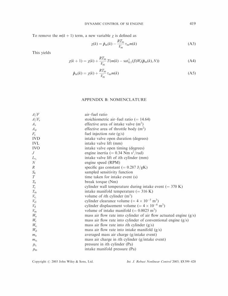
APPENDIX B: NOMENCLATURE

A=F air–fuel ratioA=Fs stoichiometric air–fuel ratio ð¼ 14:64ÞAv effective area of intake valve ðm2ÞAf effective area of throttle body ðm2ÞFc fuel injection rate (g/s)IVD intake valve open duration (degrees)IVL intake valve lift (mm)IVO intake valve open timing (degrees)J engine inertia ð¼ 0:34 Nm s2=radÞLvi intake valve lift of ith cylinder (mm)N engine speed (RPM)R specific gas constant ð¼ 0:287 J=gKÞSk sampled sensitivity functionT time taken for intake event (s)Tb break torque (Nm)Tc cylinder wall temperature during intake event ð¼ 370 KÞTm intake manifold temperature ð¼ 316 KÞVci volume of ith cylinder ðm3ÞVcl cylinder clearance volume ð¼ 4� 10�5 m3ÞVd cylinder displacement volume ð¼ 4� 10�4 m3ÞVm volume of intake manifold ð¼ 0:0025 m3ÞWa mass air flow rate into cylinder of air flow actuated engine (g/s)Wc mass air flow rate into cylinder of conventional engine (g/s)Wci mass air flow rate into ith cylinder (g/s)Wf mass air flow rate into intake manifold (g/s)ma averaged mass air charge (g/intake event)mai mass air charge in ith cylinder (g/intake event)pci pressure in ith cylinder (Pa)pm intake manifold pressure (Pa)



p0 atmospheric pressure ð100 kPaÞr reference torque (Nm)t time (s)b effective area factor of intake valvez inverted fuel injection rate (s/g), 1=Fcy crank-angle (degrees)f primary throttle angle (degrees)tm time constant of MAF sensor ð¼ 0:13 sÞtr time constant of reference torque ð¼ 0:05 sÞts time constant of EGO sensor ð¼ 0:20 sÞk; c1; c2 control parameters

REFERENCES

1. Emtage AL, Lawson PA, Passmore MA, Lucas GG, Adcock PL. The development of an automotive drive-by-wirethrottle system as a research tool. SAE Paper, No. 910081, 1991.

2. Bidan P, Boverie S, Chaumerliac V. Nonlinear control of a spark-ignition engine. IEEE Transactions on ControlSystems Technology 1995; 3(1):4–13.

3. Stefanopoulou AG. Modeling and control of advanced technology engines. Ph.D. Thesis, University of Michigan,1996.

4. Ashhab MS, Stefanopoulou AG, Cook JA, Levin M. Camless engine control for robust unthrottled operation. SAEPaper, No. 981031, 1998.

5. Stefanopoulou AG, Cook JA, Grizzle JW, Freudenburg JS. Joint air–fuel ratio and torque regulation usingsecondary cylinder air flow actuators. ASME Journal of Dynamics Systems, Measurement, and Control, to appear(see also Stefanopoulou, AG, Grizzle, JW, Freudenburg, JS. Engine air–fuel ratio and torque control using secondarythrottles. Proc. IEEE Conference Decision and Control, Orlando, 1994; 2748–2753).

6. Vogel O, Roussopoulos K, Guzzella L, Czekaj J. Variable valve timing implemented with a secondary valve on afour cylinder SI engine. 1997 Variable Valve Actuation and Power Boost SAE Special Publications, Vol. 1258(970335) February 1997; 51–60.

7. Kang JM. Advanced Control For Fuel Economy and Emissions Improvement in Spark Ignition Engines. Ph.D. Thesis,University of Michigan, 2000.

8. Grizzle JW, Kang J-M. Discrete-time control design with positive semi-definite Lyapunov functions. Systems &Control Letters 2001; 43:287–292.

9. Ashhab MS, Stefanopoulou AG, Cook JA, Levin MB. Control-oriented model for camless intake process (part I).ASME Journal of Dynamic Systems, Measurement, and Control, 2000; 122:122–130.

10. Heywood JB. Internal Combustion Engine. McGraw-Hill: New York, 1988.11. Crossley PR, Cook JA. A nonlinear model for drivetrain system development. In IEE Conference ‘Control 91’,

Vol. 2. March 1991; 921–925. IEE Conference Publication 332: Edinburgh, U.K.12. Cook JA, Powell BK. Discrete simplified external linearization and analytical comparison of IC engine families.

In Proceedings of American Control Conference, Minneapolis, June 1987; 325–333.13. Yurkovich S, Simpson M. Comparative analysis for idle speed control: a crank-angle domain viewpoint.

In Proceedings of American Control Conference, New Mexico, June 1997; 278–283.14. Bitar S, Probst JS, Garshelis I. Development of a magnetoelastic torque sensor for formula 1 and champ car racing

applications. SAE Paper, No. 2000-01-0085, 2000.15. Sontag ED. A ‘universal’ construction of Artstein’s theorem on nonlinear stabilization. Systems & Control Letters

1989; 13:117–123.16. Grizzle JW, Cook JA, Milam WP. Improved transient air–fuel ratio control using air charge estimator.

In Proceedings of 1994 American Control Conference, Vol. 2. June 1994; 1568–1572.17. Lakshmikantham V, Trigiante D. Theory of Difference Equation: Numerical Methods and Applications. Academic

Press: New York, 1988.18. Rugh WJ. Linear System Theory (2nd edn). Prentice-Hall: Englewood Cliffs, NJ, 1996.19. Aquino CF. Transient A/F control characteristics of the 5 l central injection engine. SAE Paper, No. 810494, 1981.



dynamic control of a si engine with variable intake valve

Documents