dynamic characteristics of an offshore · pdf filedynamic characteristics of an offshore wind...

S.J. Choi & A. Sarkar, et al., Int. J. Comp. Meth. and Exp. Meas., Vol. 2, No. 3 (2014) 280–297

© 2014 WIT Press, www.witpress.comISSN: 2041-9031 (paper format), ISSN: 2041-904X (online), http://journals.witpress.comDOI: 10.2495/SAFE-V2-N3-280-297

DYNAMIC CHARACTERISTICS OF AN OFFSHORE WIND TURBINE WITH BREAKING WAVE AND WIND LOAD

S.J. CHOI & A. SARKARDepartment of Mechanical and Structural Engineering and Material Science, University of Stavanger, Norway.

ABSTRACTIn this paper, the response characteristics of an offshore wind turbine (OWT) structure under breaking wave forces and wind forces are studied. A 3D numerical model, based on solving the viscous and incompressible Navier–Stokes equations and the volume of fl uid method, is employed to estimate the breaking wave forces on an OWT structure (6.0-m diameter monopile). The calculated wave forces are then applied with the wind forces on the OWT structure modeled in the computer program HAWC2 to understand the nature of its response. The effects from the aerodynamic damping and the foundation fl exibility on the structure’s response are also discussed.Keywords: breaking waves, offshore wind turbine, 3D numerical model.

1 INTRODUCTIONIn recent years, a large number of fi xed offshore wind turbines (OWT), which are supported by monopiles, tripod structures, and jacket structures, have been planned or constructed in shallow waters to capture the abundant wind energy source. Among them, a ‘monopile-transi-tion piece-tower’ type of structure seems to be preferred to support an OWT in shallow waters. For the design of a monopile structure installed on a fl at bottom, the Morison equation has generally been used to estimate wave forces on the structure. Moreover, as the frequencies of the environmental loads on a structure generally stay away from the structure’s natural fre-quency, the vibration of the structure is not a ‘major’ problem in the designing stage of the structure. However, in the case where an OWT structure is installed in a submerged shoal, the water waves may experience severely nonlinear wave deformations on their propagation, and the nonlinear waves generated toward the structure can give rise to higher local pressures and impulsive forces on the structure. Because the breaking wave impact forces normally act in a very short time, this can also cause large horizontal accelerations at the nacelle. Furthermore, the repeated occurrence of breaking waves in every season can potentially affect the fatigue life of the structure. Therefore, the accurate estimation of breaking wave impact forces and dynamic responses induced by the forces is of great importance.

Several researchers have investigated breaking wave impact forces and the dynamic responses induced by the forces throughout the numerical and experimental approaches. Hu and Kashiwagi [1] applied the Constrained Interpolation Profi le (CIP) method for studying the wave impact phenomena and violent wave–structure interactions. Christiansen et al. [2] studied the wave run-up and the extreme wave forces on an OWT foundation under the plunging breaker by using Navier–Stokes solver. Marino et al. [3] presented a numerical procedure by using Boundary Element Method (BEM)–MEL (Mixed Eulerian–Lagrangian) to simulate the extreme response of an OWT structure. Bredmose et al. [4] used a focused wave technique in Open-Foam to estimate the breaking wave impact forces on a cylindrical pile. Mokrani et al. [5] used a NS-VOF approach to study the slamming forces on a vertical wall. The wave impact on a rectangular column using smoothed particle hydrodynamics (SPH) was studied by Cummins et al. [6]. However, although various researchers have stud-ied the breaking wave impact forces on the structure, little information is currently available

S.J. Choi & A. Sarkar, et al., Int. J. Comp. Meth. and Exp. Meas., Vol. 2, No. 3 (2014) 281

in the literature on the dynamic behavior of an OWT structure under the action of the break-ing waves. Recently, several researchers have studied the dynamic responses of an OWT structure under breaking waves throughout experimental approaches. Rogers [7] studied an OWT structure encountering only the breaking waves and concluded that such forces can cause signifi cant dynamic magnifi cation of the structure’s response. Ridder et al. [8] observed large accelerations at the level of the nacelle in breaking waves, and they point out the neces-sity of studying the dynamic behavior of an OWT structure. However, the effect of wind forces with waves, aerodynamic damping, and the foundation fl exibility on the dynamic behavior of the structure is not studied in their paper.

The objective of this paper is to understand the general dynamic behavior of an OWT struc-ture under the actions of breaking wave forces and wind forces, and to point out how the aerodynamic damping and the foundation fl exibility can affect the nacelle vibration under such load cases. To achieve the purpose of the present study, we used a combination of a com-putational fl uid dynamics (CFD) model (in the hydrodynamic part) and a structural analysis model (in the structural part). In the hydrodynamic part, a 3D Navier–Stokes solver, based on viscous and incompressible momentum equations for a two-phase fl ow model and the volume of fl uid (VOF) method, is employed to estimate the breaking wave impact forces on an OWT structure. The 3D numerical model is fi rst validated by comparing with the results of the hydraulic model tests previously undertaken by Irschik et al. [9]. The breaking wave impact forces on an OWT structure (6.0-m diameter mono-pile) are then calculated, and the computed results are applied on the OWT structure modeled in a structural analysis model. In the struc-tural part, HAWC2 is employed to predict the dynamic responses induced by the breaking wave forces and wind forces. The foundation of the OWT structure is modeled by using three different approaches; these are: (i) fi xity at the mudline, (ii) fi xity at a depth of two times the pile diameter, and (iii) with distributed springs modeled by following the API guidelines. Moreover, three wind related conditions: (i) no aerodynamic damping and no wind, (ii) with aerodynamic damping and no wind, and (iii) with aerodynamic damping and operating wind of 8.0 m/s, are considered to study the effects from the aerodynamic damping.

2 HYDRODYNAMIC MODEL

2.1 Governing equations

Assuming that the two fl uids (water and air) are viscous, incompressible, and immiscible, the fl uid fl ow is governed by the continuity equation and the modifi ed Navier–Stokes equations

∂ ∂∂

+ + =∂ ∂ ∂

*( ) ( )( ) y zxm v m wm u

qx y z

(1)

∂ ∂ ∂ ∂+ + +∂ ∂ ∂ ∂v x y zu u u um m u m v m wt x y z

{ ( 2 )} { ( 2 )}t t

∧ ∧∧

∂ ∂ ∂= − + − + + − + +∂ ∂ ∂

vx xx xx y xy xy

m p m v D m v Dx x yp

(2)

*2{ ( 2 )}

3t

∧∧

∧∂ ∂− + + −∂ ∂

s xz xz xz

F m v qm v Dz xp

282 S.J. Choi & A. Sarkar, et al., Int. J. Comp. Meth. and Exp. Meas., Vol. 2, No. 3 (2014)

∂ ∂ ∂ ∂+ + +∂ ∂ ∂ ∂v x vy zv v v vm m u m v m wt x y z

{ ( 2 )} { ( 2 )}t t

∧ ∧∧

∂ ∂ ∂= − + − + + − + +∂ ∂ ∂

vx yx yx y yy yy

m p m v D m v Dy x yp

*2{ ( 2 )}

3t

∧∧

∧∂ ∂+ − + + −∂ ∂

ysz yz yz

m vF qm v Dz yp

(3)

∂ ∂ ∂ ∂+ + +∂ ∂ ∂ ∂v x y zw w w wm m u m v m wt x y z

{ ( 2 )} { ( 2 )}t t∧ ∧

∧∂ ∂ ∂= − + − + + − + +∂ ∂ ∂

vx zx zx y zy zy

m p m v D m v Dz x yp

*2{ ( 2 )}

3t l

∧∧

∧∂ ∂+ − + + − − −∂ ∂

s zz zz zz v

F m v qm v D m g wz zp

(4)

where t is the time; p is the pressure; u, v, and w are the velocity components in each direc-tion, respectively; g is the gravitational acceleration; mv is the ratio of the fractional volume open to the fl ow; mx, my, and m are the ratios of the fractional area open to the fl ow in each direction, respectively; tij is the turbulent stress based on the Smagorinsky SGS model (In this study, the Smagorinsky’s constant (=0.173) is used.) [10]; Dij is the stress rate tensor; Fs is the surface tension force based on the continuum surface force (CSF) model; l is the wave dissipation factor that equals zero except in the added dissipation zone; r̂ is the fl uid density; ̂v is the fl uid kinematic molecular viscosity; and q* is the source term required to generate waves assigned only at the source position (x = x3), defi ned as = Δ* ( , ) / sq q z t x , where q is the fl ux density and Δxs is the mesh width at the source position. To prevent an abrupt oscillation of the water surface at the start of wave generation, the fl ux density, q, is gradually increased for the initial three wave periods using an exponential function given by

{ } h h

h h

⎧ − − + + ≤⎪

= ⎨⎪ + + ≥⎩

0 0

0 0

1 exp( 2 / ) 2 ( ) / ( ) : / 3

2 ( ) / ( ) : / 3

s

s

t T U h h t Tq

U h h t T (5)

where T is the wave period, U0 and h0 are the horizontal water particle velocity and the free surface elevation computed by the stream function wave theory, respectively, hs is the free surface elevation computed at the source position, and h is the water depth.

2.2 Free surface elevation

To track the interface between two-phase fl ows, we use the original VOF method developed by Hirt and Nichols [11]. Although the original VOF method uses the simplifi ed line inter-face calculation in interface reconstruction, its applicability has been demonstrated by


many researchers [12,13]. In the VOF method, the interface between the water and the air phase is modeled according to the VOF function, F, i.e. in the VOF method the volume of water in each cell evolves over time instead of the free surface itself being tracking. The advection of the VOF function is obtained by solving the conservation of fl uid mass in each cell as follows:

∂ ∂∂ ∂+ + + =

∂ ∂ ∂ ∂*( ) ( )( ) ( ) y zv x

m vF m wFm F m uFFq

t x y z

(6)

2.3 Boundary conditions

To treat the boundary of the calculation area, appropriate boundary conditions were adopted on the solid boundary and the lateral boundaries. There was no need to apply the free-sur-face boundary condition because the water and the air phase were modeled as a fl uid in the two-phase fl ow model. For this reason, the dynamic boundary condition is automatically satisfi ed, whereas the kinematic boundary condition is satisfi ed by tracking the VOF func-tion. As for the open boundary conditions, fi ctitious dissipation zones that were proposed by Hinatsu [14] were added at both the ends of the computational domain to control the refl ected waves. To obtain an artifi cial damping effect, grids in the added fi ctitious dissipation zones were gradually coarsened toward the outmost open boundaries. Moreover, a non-gradient boundary condition was employed at the outer edges of the added fi ctitious dissipation zones. The pressure-constant condition was applied to the top boundary condition. An impermeable condition (for normal velocities) and a slip condition (for tangential veloci-ties) were imposed to treat the bottom boundary condition and the obstacle boundary condition, respectively.

2.4 Method of solution

Finite difference methods are used to calculate the values of the governing equations and the advection equation for the VOF function. Variables are staggered, which means that the pres-sure (p), the wave source function (q*), and the VOF function (F) are computed at the cell center, whereas the velocity components (u, v, w) are computed at the center of the cell face. The continuity equation is discretized by the central difference method. As for the discretiza-tion of the Navier–Stokes equations, the forward difference method for time derivative terms, the CIP method for the advection terms, and the central difference method for the non-advec-tion terms are employed. The velocity components (u, v, w) and the pressure (p) at the new time step can be estimated using the discretized momentum equations and suitable boundary conditions. However, the new time velocity components, which are estimated using the dis-cretized momentum equations, do not generally satisfy the continuity equation in a control volume. Therefore, the Simplifi ed Maker and Cell (SMAC) method [15] is incorporated to iteratively adjust the velocities and the pressure in each cell until the continuity equation is reasonably satisfi ed. In the SMAC method, the pressure correction can be obtained by solv-ing a Poisson Pressure Equation (PPE). Then, the correct velocities at new time steps can be updated using the pressure correction computed by the PPE. In this study, the PPE is solved by the AP-AMG (Algebraic Multigrid) solver, which was developed by Iwamura, Allied Engineering [16]. After the correct velocity components and pressure have been determined,


the new free surface confi guration is tracked by solving the advection equation for the VOF function using the updated velocity components.

3 VALIDATION OF 3D NUMERICAL MODEL

3.1 Model description

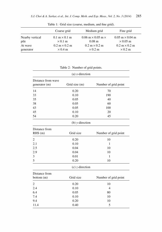
As previously mentioned, the 3D numerical model is validated by using the results of the hydraulic model test previously undertaken by Irschik et al. [9]. A numerical wave tank (NWT) similar to the hydraulic model test tank (Fig. 1) is used. The NWT has a length of 54.0 m, a width of 5.0 m, and a height of 11.4 m. The water depth at the front of the wave generator is 3.8 m, which reduces to 1.5 m at the berm with a slope of 1 in 10. Wave dissipa-tion zones of length 2 L (L = the wave length) are added on the two sides of the computational domain. An incident wave condition (regular wave, 1.30-m wave height and 4.0-s wave period) is used to create breaking waves at the location of the pile. A vertical pile with a diameter of 0.70 m is located at the edge of the slope, as shown in Fig. 1. Nineteen numerical wave gauges are used to measure the water surface elevations. Moreover, 19 numerical pres-sure gauges are uniformly distributed along the frontline of the cylinder with a spacing of 0.2 m. The breaking wave forces are obtained by the integration of the pressure distribution over the wetted surface of the pile. The model is run for 40 s (i.e. 10 wave periods). The time increment is automatically adjusted at each time step to obtain maximum effi ciency. A grid refi nement test is performed to check the sensitivity of the grid spacing. Three grid sizes are tested to check the convergence of the results from the NWT, which are: a coarse grid, a medium grid, and a fi ne grid (see Table 1). The fi ne grid contains approximately 2.6 million cells (x-direction: 525 cells, y-direction: 42 cells, and z-direction: 119 cells), as shown in Table 2 and Fig. 2. The computation has been performed on six parallel dual core processors and the total computational time is about 5 days. More details about the model description can be found in [17].

Figure 1: Schematic illustration of NWT and location of pressure gauges P5, P6, and P7 in NWT.


Table 1: Grid size (coarse, medium, and fi ne grid).

Coarse grid Medium grid Fine grid

Nearby vertical pile

0.1 m × 0.1 m × 0.1 m

0.06 m × 0.05 m × 0.08 m

0.05 m × 0.04 m × 0.05 m

At wave generator

0.2 m × 0.2 m × 0.4 m

0.2 m × 0.2 m × 0.2 m

0.2 m × 0.2 m × 0.2 m

Table 2: Number of grid points.

(a) x-direction

Distance from wave generator (m) Grid size (m) Number of grid point

14 0.20 7033 0.10 19035 0.05 4038 0.05 6043 0.05 10045 0.10 2054 0.20 45

(b) y-direction

Distance from RHS (m) Grid size Number of grid point

2 0.20 102.1 0.10 12.5 0.04 102.9 0.04 103 0.01 15 0.20 10

(c) z-direction

Distance from bottom (m) Grid size Number of grid point

2 0.20 102.4 0.10 46.4 0.05 807.4 0.10 109.4 0.20 1011.4 0.40 5


3.2 Comparison between the numerical and the experimental results

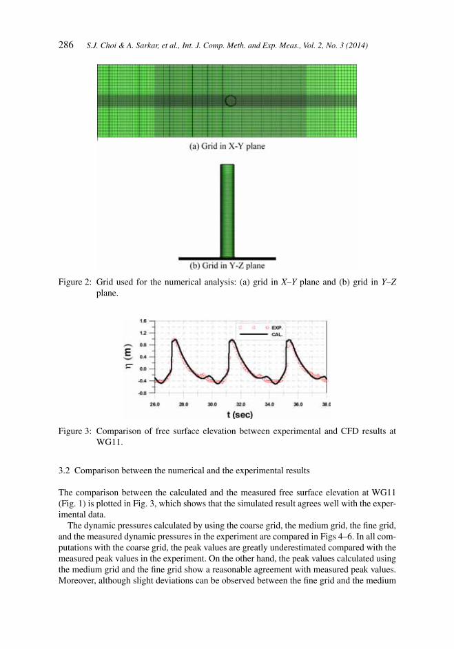
The comparison between the calculated and the measured free surface elevation at WG11 (Fig. 1) is plotted in Fig. 3, which shows that the simulated result agrees well with the exper-imental data.

The dynamic pressures calculated by using the coarse grid, the medium grid, the fi ne grid, and the measured dynamic pressures in the experiment are compared in Figs 4–6. In all com-putations with the coarse grid, the peak values are greatly underestimated compared with the measured peak values in the experiment. On the other hand, the peak values calculated using the medium grid and the fi ne grid show a reasonable agreement with measured peak values. Moreover, although slight deviations can be observed between the fi ne grid and the medium

Figure 2: Grid used for the numerical analysis: (a) grid in X–Y plane and (b) grid in Y–Z plane.

Figure 3: Comparison of free surface elevation between experimental and CFD results at WG11.


grid results, there is good overall agreement. From the comparisons, it can be concluded that the accuracy of the simulation results depends greatly on the cell resolution. Meanwhile, in P5 and P6 (see Figs 4 and 5), the computed rise-times are signifi cantly smaller than the meas-ured rise-times, even though the computed fall-times show a reasonable agreement with the measured fall-times. The ‘rise-time’ depends greatly on the air entrainment, the compressibil-ity, and the motion of the structure. However, as the used CFD model is based on incompressible momentum equations and the monopile installed in the NWT is modeled as a rigid object, the numerical model does not seem to correctly compute the rise-time of the local pressures.

The vertical pile is modeled as a rigid object in the numerical model. However, in the experiment, the pile has to move to induce suffi cient strain in the force transducers (i.e. mov-ing object). The total force time series obtained from the experiment, when converted into frequency domain, shows a peak that corresponds to the natural frequency of the structure (20.0 Hz). This is expected, since the natural frequency of the structure is close to the break-ing wave impact force duration. Hence, to compare with the numerical results, the total impact force data obtained from the experiment have to be fi ltered to remove the amplifying effect due to the structure’s vibration. A low pass fi lter and empirical mode decomposition (EMD) are used to remove the dynamic amplifying effect in experimental data. Figure 6 (gray line) shows the wave forces fi ltered by a FFT low pass fi lter (cut-off frequency: 20 Hz). However, it seems that residual responses still exist in the fi ltered wave force data. EMD is used to completely remove the residual responses in the fi ltered wave force data. It is observed

Figure 4: Comparison of dynamic pressures using the coarse grid, using the medium grid, using the fi ne grid, and the measured dynamic pressures at P5.



that the high-frequency oscillation (i.e. the effect of dynamic amplifi cation) in the measured wave force data is completely removed by using the low pass fi lter and EMD (see red dash line in Fig. 7).

Figure 8 shows the comparison of wave forces calculated by a low pass fi lter and EMD and numerical result. The agreement between the measured result (i.e. the effect of dynamic amplifi cation is completely removed) and the CFD result is good, even though there is only a small gap in the falling time. The reason for the gap in the falling time can be attributed to the large amount of air bubbles, which may be entrained in the water after the waves are


Figure 7: Comparison of wave force fi ltered by FFT low pass fi lter and the wave forces calculated by FFT low pass fi lter and EMD.

Figure 8: Comparison of wave force calculated by low pass fi lter + EMD and numerical result.


broken. This can decrease the effective density of the water (and the velocity of sound in the water), which can reduce the wave forces on the ‘fall-time’ to some extent. This discrepancy may be reduced by using a 3D numerical model for the compressible fl ow.

From the above results, it can be concluded that the 3D numerical model is a useful tool for predicting the breaking wave impact forces on a structure. Hence, it is employed to esti-mate the impact forces on a monopile of 6.0-m diameter, and the computed results are later applied on the OWT structure modeled in a structural analysis model to study the nature of its response.

4 STRUCTURAL MODEL

4.1 Governing equations

The software HAWC2 [18] is employed to predict the dynamic responses induced by the breaking wave forces and wind forces. In HAWC2, the OWT structure is modeled with a multibody formulation using the fl oating frame of reference approach, where each body is modeled with Timoshenko beam element(s) [18]. Following Shabana [19], the equations of motion of a structure in a fl oating frame of reference can be expressed as

l+ + = + = ⋅⋅⋅..

1,2, ,ii i i i T i i

e v bqM q K q C Q Q i n (7)

where Mi is mass matrix of body i in the multi-body system, Ki is the stiffness matrix of the ith body, qi

is the total vector of generalized coordinates of body i, Qie is the vector general-

ized forces associated with generalized coordinate for body i, Qiv is the quadratic velocity

vector resulting from the derivative of the kinetic energy with respect to time and body coor-dinate, and nb is the total number of bodies. In eqn (7), Qi

v contains the gyroscopic and Coriolis force components, while other generalized forces are included inQi

e.

4.2 Wind excitation

In engineering problems, wind is normally defi ned by the combination of a mean wind speed and turbulence. The mean wind speed varies with time, which can be described by Weibull distribution. Von Karman’s isotropic energy spectrum is used to model the wind, whereas the Mann model [20] is used for modeling the turbulence. The blade element momentum (BEM) theory is used to estimate the wind forces on blades.

4.3 Application of breaking wave impact forces in the structural model

For applying the breaking wave impact forces on the OWT structure modeled in HAWC2, two nodes (A and B) are assumed on the monopile (see Fig. 9): node A lies above the wave breaking zone, whereas node B is located close to the mudline. The length between these nodes is divided into N segments, and the breaking wave impact forces calculated by the CFD model are applied on each segment. These forces are then converted into the equivalent loads acting on the two nodes (FMA, FRA, FMB, and FRB; see Fig. 9). These equivalent load time series are inserted in the HAWC2 model to compute the dynamic response of the OWT structure.


4.4 Foundation modeling

An OWT structure is essentially a cantilever structure orientated vertically and supported by the seabed. Hence, a realistic model representing the foundation plays an important role in the reliability of the results obtained from a numerical analysis. There are various ways of modeling the soil–structure interaction. Three different approaches are adopted in the paper; these are: (1) pile fi xed at the mudline, (2) pile fi xed at a depth two times the pile diameter below the mudline, and (3) pile fl exibility modeled by distributed lateral springs, which are attached to the pile below the mudline.

4.5 Damping in the model

The sources of damping in an OWT can be broadly classifi ed as: structural damping, aerody-namic damping, hydrodynamic damping, and soil damping. In general, the hydrodynamic damping for such cases is expected to be small as the water depth is small, and the motion of the structure is very small (near the support). Devriendt et al. [21] have presented the meas-ured damping on an actual OWT structure. Following this, the damping can be taken as 1.1% approximately (includes structural, soil, and non-breaking hydrodynamic damping and excludes the aerodynamic damping). On the other hand, a logarithmic decrement in the range of 10–20% is reported by Tarp-Johansen [22] for a 3 MW OWT, which includes all four types of damping listed above.

In this study, the natural frequency of the OWT structure (fs) is estimated to be 0.23 Hz (i.e. natural period 4.34 s). This is found to be approximately the same for all three different foundation conditions. To estimate the damping in the model, a free vibration study is carried out on the structural model by using a ramp load. It is observed that the model incorporates 1% damping when aerodynamic and hydrodynamic damping are excluded (i.e. mainly struc-tural and soil damping), and 23% of logarithmic decrement when aerodynamic damping is included along with the other types. This indicates that realistic damping is included in the model. Any hydrodynamic damping due to the breaking waves is included in the output of the NS solver.

Figure 9: Application of the computed breaking wave impact forces in HAWC2.


5 APPLICATION OF A STRUCTURAL MODEL

5.1 Model description

The bottom geometry used in the study is shown in Fig. 10. The water depths are at 30.4 m in the offshore region and 12.0 m in the submerged shoal. The slope of the bottom is one divided by ten. A vertical pile with a diameter of 6.0 m is located at the edge of the slope. An incident wave condition (wave height, H = 10.4 m and wave period, T = 11.3 s) is used for making breaking waves at the structural position. For the wave condition, the surf similarity parameter is found to be 0.44; i.e. the breaking wave lies almost on the boundary of spilling to plunging type breaker. The breaking wave forces computed by the numerical model are applied on the OWT structure modeled in HAWC2, which is used to predict the dynamic response induced by the breaking wave forces and the wind forces. The major structural properties used in HAWC2 are presented in Table 3. Moreover, three wind states are consid-ered in this study; these are: (1) no aerodynamic damping and no wind, (2) with aerodynamic damping and no wind, and (3) with aerodynamic damping and with normal wind speed of 8.0 m/s acting in the same direction as the breaking waves.

Table 3: Major properties of the turbine.

Rating 5 MWRotor confi guration 3 bladedHub height 90 m from MWLCut-in, rated, and cut-out wind speed 3 m/s, 11.4 m/s, 25 m/sCue-in, rated rotor speed 6.9 rpm, 12.1 rpmRotor mass 110 TeNacelle mass 240 TeMonopile foundation Ø 6.0 m (thickness = 0.06

m), extends up to 36 m below mudline

Material properties of steel E = 210 GPa, G = 80.8 GPaSoil Sand

Figure 10: Bottom geometry and monopile structure used in the study.


6 RESULTS AND DISCUSSIONIt can be shown that the dynamic amplifi cation factor (DAF) of the response of a structure under the action of an impulsive load is governed by the natural frequency of the structure, the duration of the impulse, and its shape. For example, in the case of a rectangular pulse, a maximum DAF = 2 will result when the impulse duration is more than or equal to half of the natural period of the structure. In this study, the breaking wave impact duration is estimated by using the model presented in [23], as shown in eqn (8)

= 12d

w

DtC

(8)

where td is the breaking wave impact duration, D is the diameter of the pile (6.0 m), and Cw is the wave celerity (14.48 m/s for the case studied here). The estimated impact duration is 0.207 s, which is much smaller when compared with the fi rst natural period of the structure modeled here (4.34 s). Hence, a large DAF induced by the breaking wave impact forces is not expected.

In general, the frequency of the breaking waves (fB) is the same as the non-breaking regular wave frequency coming from the deeper water, which is 0.088 Hz (11.3 s). When the total breaking wave force time series (Fig. 11) is converted into frequency domain, it shows the presence of higher harmonics (n × fB), which can be observed in Fig. 12.

Figure 12 shows the importance of the fi rst three harmonics on the dynamics of the struc-ture, as they not only exist in the vicinity of the structure’s natural frequency but also contain

Figure 11: Time series of total breaking wave force on 6.0-m diameter monopile.

Figure 12: Total breaking wave force on 6.0-m diameter monopile in frequency domain.


a signifi cant amount of energy. As a general approach, OWT structures are designed in such a way that the fi rst natural frequency remains away from the range of the excitation frequen-cies (i.e. the regular wave frequencies and the blade passing frequencies). Therefore, this is considered to avoid resonating vibration in the structure. On the other hand, in the case of breaking wave impact force on the structure, due to the presence of higher harmonics in the force spectrum (i.e. fi rst three harmonics, see Fig. 12), a large structural response would occur.

Figures 13 and 14 show the response of the nacelle’s displacement in frequency domain for fl exible and fi xed foundations, with and without the aerodynamic damping. They show prom-inent peak responses, which correspond to the incoming wave frequency (fB) and its higher harmonics (n × fB). The largest peak in the structure’s response corresponds to the fi rst higher harmonic (i.e. 2 × fB, 0.176 Hz) of the incoming wave frequency, as it is close to the natural frequency of the structure (0.23 Hz). A smaller peak appearing at the structure’s natural fre-quency is somewhat affected by the presence of the aerodynamic damping.

It is also noticed that the sizes of the peaks increase when the structure is modeled with a fl exible foundation instead of a fi xed foundation, even though the natural frequencies are almost the same. This is evident since the fl exibility of the foundation allows some rotation of the tower at the seabed level, which results in larger motion at the nacelle level. Hence, a fi xed foundation model may not be able to provide a realistic estimation of the response of the structure. Figures 15–17 present the comparisons of the base bending moment and the nacelle acceleration, with and without the aerodynamic damping, at the instant when a

Figure 13: Nacelle displacement for fl exible foundation in frequency domain.

Figure 14: Nacelle displacement for foundation fi xed at a depth two times the pile diameter in frequency domain.


breaking wave hits the structure. The results show that the responses are not appreciably affected by the presence of the aerodynamic damping. The fl exible foundation shows largest acceleration among the three foundation cases, whereas the base bending moment is slightly larger for the fi xed foundations compared with the fl exible foundation. For this particular structure and load case, the maximum estimated acceleration at the nacelle level is found to be 2.0 m/s2.

Figures 18 and 19 show the same plots for the case with a normal wind speed of 8.0 m/s, and similar observations are made. It is also noticed that small vibrations, like ringing of a bell, occurring after the structure is hit by a breaking wave, decay rather quickly.

Figure 15: Base bending moment without aerodynamic damping.

Figure 16: Nacelle acceleration without aerodynamic damping.

Figure 17: Nacelle acceleration with aerodynamic damping.


7 CONCLUSIONIn this paper, the response characteristics of an OWT structure under the breaking wave impact force and the wind force are studied. The major conclusions, based on the numerical results, can be summed up as follows:

1. The breaking wave impact force is estimated by the 3D numerical model. The numerical model is fi rst validated with experimental results, and good agreements between the two results are observed. Therefore, the 3D numerical model can be used to obtain a reliable estimation of the breaking wave impact forces on a monopile.

2. It is obvious that the peak response of the structure is dependent on its natural frequency and the impact load duration time. In this study, a large DAF is not expected because the natural period of the OWT structure is much larger than the duration of the breaking wave impact forces. However, it is observed that the breaking wave impact force consists of the incident wave frequency and its higher harmonics. Apart from the frequency of the incident wave, its fi rst and second multiple is found to contain a signifi cant amount of energy. If any of these coincides with the natural frequency of the structure, a large structural response would occur. The maximum acceleration at the nacelle level, for this particular structure and input wave condition, is estimated to be 2.0 m/s2.

3. It is also observed that the numerical results depend on modeling the foundation fl ex-ibility. A model with fl exible foundation predicts larger acceleration at the nacelle level compared with a fi xed foundation.

Figure 18: Nacelle acceleration with 8 m/s wind speed.

Figure 19: Base bending moment with 8 m/s wind speed.


4. The effect of the aerodynamic damping on the peak response at the nacelle level is found to be negligible. Some relatively quick vibrations, resembling the ringing of a bell, occurring just after a breaking wave hits the structure, is observed, and this is found to decay rather quickly.

ACKNOWLEDGEMENTSThis research is supported by the Research Council of Norway and NORCOWE. The authors are thankful to Prof. Ove T. Gudmestad, of the University of Stavanger, for his encourage-ment during this study. The experimental data are provided by Lisham Bonakdar and Prof. Hocine Oumeraci, TU Braunschweig, Germany. The AP-AMG solver is provided by Chihiro Iwamura, Allied Engineering Corporation, Japan.

REFERENCES[1] Hu, C. & Kashiwagi, M., A CIP-based method for numerical simulations of violent

free-surface fl ows. Journal of Marine Science and Technology, 9, pp. 143–157, 2004. doi: http://dx.doi.org/10.1007/s00773-004-0180-z

[2] Christiansen, E.D., Bredmose, H. & Hansen, E.A., Extreme wave forces and wave run-up on offshore wind turbine foundations. Copenhagen Offshore Wind, Copenhagen, 2005.

[3] Marino, E., Borri, C. & Peil, U., Offshore wind turbine: a wind-fully nonlinear waves integrated model. The 5th International Symposium on Computational Wind Eng (CWE2010), 2010.

[4] Bredmose, H. & Jacobsen, N.G., Breaking wave impacts on offshore wind turbine foun-dation: focused wave groups and CFD. Proceedings of the ASME 2010 29th Interna-tional Conference on Ocean, Offshore and Arctic Eng (OMAE), Shanghai, China, 2010.

[5] Mokrani, C., Abadie, S., Grilli, S. & Zibouche, K., Numerical simulation of the impact of a plunging breaker on a vertical structure and subsequent over topping event using Navier–Stoke’s VOF model. Proceedings of the 20th International Offshore and Polar Engineering Conference, Beijing, China, pp. 729–736, 2010.

[6] Cummins, S.J., Silvester, T.B. & Cleary, P.W., Three-dimensional wave impact on a rigid structure using smoothed particle hydrodynamics. International Jour-nal of Numerical Methods in Fluids, 68, pp. 1471–1496, 2011. doi: http://dx.doi.org/10.1002/fl d.2539

[7] Rogers, N., Structural dynamics of offshore wind turbines subject to extreme wave loading. Proceedings of the 20th BWEA Annual Conference, 1998.

[8] Ridder, E.J., Aalberts, P., Berg, J., Buchner, B. & Peeringa, J., The dynamic response of an offshore wind turbine with realistic fl exibility to breaking wave impact. Proceed-ings of the ASME 2011 30th International Conference on Ocean, Offshore and Arctic Engineering, Rotterdam, The Netherlands, 2011.

[9] Irschik, K., Sparboom, U. & Oumeraci, H., Breaking wave characteristics for the load-ing of a slender pile. Proceedings of the 28th International Conference on Coastal Engineering, pp. 1341–1352, 2002.

[10] Smagorinsky J., General circulation experiments with the primitive equation. Month-ly Weather Review, 91(3), pp. 99–164, 1963. doi: http://dx.doi.org/10.1175/1520-0493(1963)091<0099:GCEWTP>2.3.CO;2

[11] Hirt, C.W. & Nichols, B.D., Volume of fl uid method for the dynamics of free boundar-ies. Journal of Computational Physics, 39(1), pp. 201–225, 1981. doi: http://dx.doi.org/10.1016/0021-9991(81)90145-5


[12] Kawasaki, K. & Iwata, K., Numerical analysis of wave breaking due to submerged breakwater in three-dimensional wave fi elds. Proceedings of the Conference of the American Society of Civil Engineers, Copenhagen, Denmark, pp. 853–866, 1998.

[13] Lee, K.H. & Mizutani, N., A numerical wave tank using direct-forcing immersed boundary method and its application to wave force on a horizontal cylinder. Coast-al Engineering Journal, 51, pp. 27–48, 2009. doi: http://dx.doi.org/10.1142/S0578563409001928

[14] Hinatsu, M., Numerical simulation of unsteady viscous nonlinear waves using moving grid systems fi tted on a free surface. Journal of the Kansai Society of Naval Architects, 217, pp. 1–11, 1992.

[15] Amsden, A.A. & Harlow, F.H., A simplifi ed MAC technique for incompressible fl uid fl ow calculation. Journal of Computational Physics, 6, pp. 322–325, 1970. doi: http://dx.doi.org/10.1016/0021-9991(70)90029-X

[16] Allied Engineering, User’s Manual for Advanced Parallel AMG Version 1.3, Allied En-gineering: Tokyo, 2011.

[17] Choi, S.J. & Gudmestad, O.T., Breaking wave forces on a vertical pile. WIT Transac-tions on the Built Environment, 129, pp. 3–12, 2013. doi: http://dx.doi.org/10.2495/FSI130011

[18] Larsen, T.J. & Hansen, A.M., How 2 HAWC2 The User’s Manual, Risø-R-1597(ver. 4-1), Risø National Laboratory: TU Denmark, Roskilde, Denmark, 2011.

[19] Shabana, A.A., Dynamics of Multibody System, 3rd edn., Cambridge University Press: University of Illinois at Chicago: New York, 1998.

[20] Mann, J., Models in Micrometeorology, Risø-R-727, Risø National Laboratory: Roskil-de, Denmark, 1994.

[21] Devriendt, C., Jordaens, P.J., Sitter, G.D. & Guillaume, P., Damping Estimation of an Offshore Wind Turbine on a Monopile Foundation. European Wind Energy Association 2012: Copenhagen, Denmark, 2012.

[22] Tarp-Johansen, N.J., Comparing sources of damping of cross-wind motion. European Offshore Wind Conference, EOW 2009, 14–16 September, Stockholm, Sweden, 2009.

[23] Goda, Y., Haranaka, S. & Kitahata, M., Study of impulsive breaking wave forces on piles. Report of Port and Harbour Research Institute, Ministry of transport, Japan, 5(6), pp. 1–30, 1966.

Note: This paper is a revised and updated paper based on paper [17] published in WIT Trans-actions on the Built Environment, Vol. 129, WIT Press, 2013.

dynamic characteristics of an offshore · pdf filedynamic characteristics of an offshore wind...

Documents