dynamic behavior of closed grinding systems and effective ... · pdf filedynamic behavior of...

Dynamic Behavior of Closed Grinding Systems and Effective PID

Parameterization TSAMATSOULIS DIMITRIS

Halyps Building Materials S.A., Italcementi Group

17th Klm Nat. Rd. Athens – Korinth

GREECE

[email protected] http://www.halyps.gr

Abstract: - The object of the present study is to investigate the dynamic of closed circuit cement mills and based on that to tune robust PID controllers applied to three actual installations. The model that has been

developed, consisting of integral part, time delay and a first order filter, is based exclusively on industrial data

sets collected in a period more than one year. The model parameters uncertainty is also assessed varying from 28% to 36% as the gain is concerning and 34% to 42% as regards the time delay. As significant sources of

model uncertainty are determined the grinding of various cement types in the same cement mill and the

decrease of the ball charge during the time. The Internal Model Control (IMC) and M - Constrained Integral

Gain Optimization (MIGO) methods are utilized to adjust the controller parameters. Specially by implementing the MIGO technique robust controllers are built deriving a daily average IAE 2.3-3% of the set

point value. Due to the high flexibility and effectiveness of MIGO, the controllers can be parameterized by

taking into account the cement type ground and the power absorbed. Subsequently the attenuation of main uncertainties leads to improvement of the regulation performance.

Key-Words: - Dynamic, Cement, Mill, Grinding, Model, Uncertainty, PID, tuning, robustness, sensitivity

1 Introduction Among the cement production processes, grinding is

very critical as far as the energy consumption is

concerned. On the other hand the grinding is very essential as to the product quality characteristics

because during this process the cement acquires a

certain composition and fineness. Because of these two reasons, grinding mostly is performed in closed

circuits, where the product of the cement mill (CM)

outlet is fed via a recycle elevator to a dynamic

separator. The high fineness stream of the separator constitutes the final circuit product, while the coarse

material returns back to CM to be ground again.

A simplified flow sheet, showing the basic components of a closed grinding system is

demonstrated in the Figure 1.

Figure 1.Closed circuit grinding system.

A contemporary cement production plant applies

a continuous and often automatic control of the production as well as of the quality. These two

operations should always be controlled and

regulated simultaneously and in combination and never as individual ones. The automatic operation

presents several advantages in comparison to the

manual one [1, 2]. In the usual automatics one of the

following has typically selected as process variable. (1) The power of the recycle elevator. (2) The return

flow rate from the separator. (3) An electronic ear in

the mill inlet. (4) The mill power or combination of the above.

Several studies describe numerous techniques of

mills automation with varying degrees of complexity. Ramasamy et al. [3], Chen et al. [4]

developed Model Predictive Control schemes for a

ball mill grinding circuit. Because of the

multivariable character, the high interaction between process variables and non – linearity always present

in closed grinding systems, control schemes of this

kind were developed [5, 6, 7, 8]. A survey of the industrial model predictive control technology has

been provided by Qin et al. [9]. The common

between all these efforts and designs is the assumption of a model describing the process

dynamics. However it has been mentioned by

Astrom et al. [10] that in the industrial process

WSEAS TRANSACTIONS on SYSTEMS and CONTROL Dimitris Samatsoulis

ISSN: 1991-8763 581 Issue 12, Volume 4, December 2009

mailto:[email protected]

http://www.halyps.gr/

control more than 95% of the control loops are of

PID type and moreover only a small portion of them operate properly as Ender [11] points out.

Frequently also the controller parameters are tuned

with trial and error [12], because of the lack of a

model or of high model uncertainty. To overcome such difficulties fuzzy PID controllers have been

also recently developed [13] and the pseudo-

equivalence with the linear PID was proven. As it was clearly stated by Astrom [14], model

uncertainty and robustness have been a central

theme in the development of the field of automatic control. Subsequently it is of high importance not

only to describe a process using a representative

model, but to estimate the parameters uncertainty as

well. This consideration can facilitate the design of a robust controller.

Two models of the dynamic behavior of closed

circuit grinding systems are developed and a detailed analysis of the model parameters

uncertainty is attempted. Actual industrial data of

three cement mills – CM5, CM6 and CM7 - of the Halyps Cement Plant are considered collected in a

long term period, where various cement types were

ground. The above analysis could lead to the design

and parameterization of a robust controller of PID type, which is usually the industrial case.

In spite of all the advances of the control during

the last decades the PID controller remains the most common one. Because of their simplicity of

implementation, these controllers are extensively

used in industrial applications [15]. In spite the

numerous papers written on tuning of PID controllers, it remains a challenge to adjust

effectively, existing and operating PID loops,

installed in grinding systems as the mentioned ones, where a detailed analysis of the dynamic behavior

has been performed.

Nyquist-like design methods are proposed to handle uncertainties in a straightforward way, as the

classical Z-N tuning (Ziegler and Nichols) [16] and

BLT method [17].

A widely applied technique to tune PID controllers is this of Internal Model Control (IMC).

Garcia, Morari and Rivera developed Internal Model

Control [18, 19, 20, 21]. Morari and Zafiriou [22] summarized Internal Model Control over a wide

range of control problems. Yamada presented a

modified IMC for unstable systems [23]. Essential also contribution had Cooper [24] and Skogestad

[25, 26] to the IMC implementation.

Another extensively applied tuning methodology

is the robust loop shaping [27, 28, 29, 30, 31]. A very effective loop shaping technique to tune PID

controllers was proven to be the called MIGO (M-

constrained integral gain optimization) [32, 33, 34,

35]. The design approach was to maximize integral gain subject to a constraint on the maximum

sensitivity. There are also other successful attempts

to design PID controllers in the frequency domain

and to characterize their performance [36, 37]. The investigation gives interesting insights and

tries to provide answer to the following question:

When is it worthwhile to do more accurate modeling, to search for enduring sources of

uncertainty and to reject them permanently if

possible? Two tuning methodologies are applied and the resulting controllers are utilized to regulate three

CM operations under highly uncertain conditions

2 Model Development In all the cases the response of the recycle elevator

power to mill fresh feed disturbances is examined.

According to Astrom et al. [38], there is a limited order of models, which can be applied to linear and

time invariant systems or systems approaching this

state. Primarily the system stability under the given

operating conditions has to be analyzed, e.g. if a step change of the fresh feed, leads to a new steady state

of the elevator power. In the opposite case the

system transfer function contains integral part. The delay time between a disturbance of the fresh feed

and the elevator response shall be investigated. To

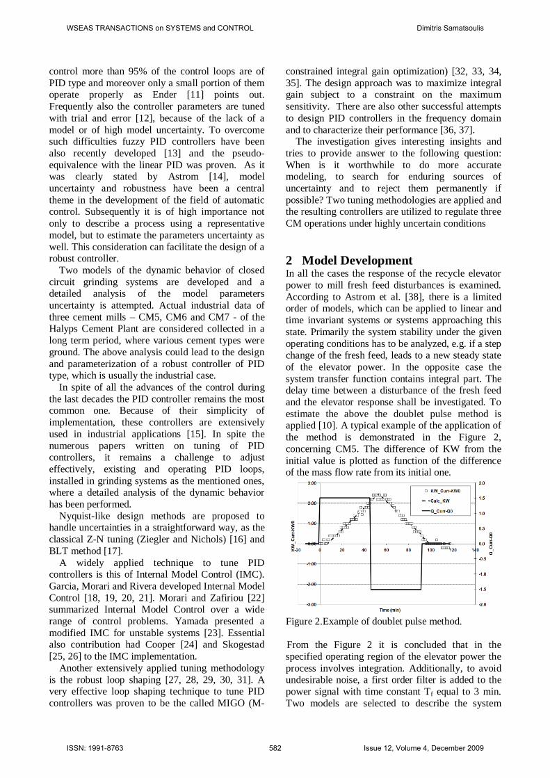
estimate the above the doublet pulse method is applied [10]. A typical example of the application of

the method is demonstrated in the Figure 2,

concerning CM5. The difference of KW from the

initial value is plotted as function of the difference of the mass flow rate from its initial one.

Figure 2.Example of doublet pulse method.

From the Figure 2 it is concluded that in the

specified operating region of the elevator power the

process involves integration. Additionally, to avoid undesirable noise, a first order filter is added to the

power signal with time constant Tf equal to 3 min.

Two models are selected to describe the system



dynamics: The first does not take into account the

first order filter and includes only the integrating action and the time delay. To compensate the

filtering action and the different system behavior

when the recycle elevator power is increasing or

decreasing, two transfer functions are designed represented in Laplace form by the equations (1),

(2).

sTdv es

kQQKWKW 1

00 )( (1)

sTdv es

kQQKWKW 2

00 )( (2)

where Q = the mass flow rate (tn/h), KW =

P/PMax∙100, the percentage of the power P of the

recycle elevator to the maximum installed power PMax, Q0 = the flow rate corresponding to power

percentage KW0 of the steady state, kv1, kv2= the

gains (h/tn) when the elevator is increasing and decreasing correspondingly and Td= the delay time

(min),.

The second model incorporates the first order

filter actually existing. Consequently the model is described by the following equation:

sTd

f

v esTs

kQQKWKW

)1()( 00 (3)

The meaning of the model parameters and variables

is exactly the same as in the first one. Apparently the two models constitute a simplification of the actual

process. If they describe adequately the CM

dynamic behavior shall be verified from the comparison between the actual and calculated

values. It must be taken into account that for the

parameterization of a controller, the simplest possible model shall be chosen. Then, the quality of

the regulation is a function of the model accuracy

[39]. It shall also be clarified that mathematical

models have been developed, describing with extraordinary adequacy the grinding process [40, 41,

42]. However frequently, due to their complicated

structure, the corresponding transfer function is extremely difficult or impossible to be derived.

By substituting the flow rate term of the above

equations with the input signal u, and the power term with the output signal e, equations (1), (2), take

the form of the equations (4), (5) respectively, while

equation (3) is transformed to the formula (6)

representing the transfer function of the process Gp for the two models under consideration:

sTdv es

k

u

e 1 (4)

sTdv es

k

u

e 2 (5)

sTd

f

v esTs

k

u

e

)1( (6)

The set of the model parameters includes the gain kv, the delay time Td, as well as the flow rate Q0 and

power KW0, corresponding to the system steady

state, under the specified any time operating conditions of the grinding circuit concerning (a)

cement type, (b) raw materials moisture and

grindability, (c) gas flows, (d) pressures, (e)

temperatures, (f) condition of the grinding media, (g) separator efficiency etc. The variety of these

conditions generates the model uncertainty as

concerns the parameters values. Therefore the first model includes six independent parameters while

the second one only four, but its form is relatively

more complicated that the first one. The first model has the advantage that simpler PID tuning

techniques can be applied, while the second

describes more accurately the process.

The model parameters are calculated by applying the convolution theorem between the input signal u

and the process variable e, expressed by the equation

(7).

t

dtgue0

)()( (7)

Where g(t) is the pulse system response. Exclusively

industrial data of routine operation of the CM are utilized. These data are sampled on-line by using

convenient software. Time intervals equal to 250

minutes of continuous mill operation are selected as individual sets of data and the parameters are

estimated for each separate set, by using a non-linear

regression technique. For this purpose software in Visual Basic for Applications was developed. As a

result, the experimental estimation of the parameters

by applying the doublet pulse method is avoided as

it presents some severe disadvantages: (a) The feed disturbance results in a disturbance in the production

process, having in parallel an impact on the product

quality. (b) As the process contains integration, the achievement of a steady state condition, required by

the method, is not easy at all. (c) To have an

estimation of the range the dynamic parameters are



varying, a large number of experiments are needed

to have a reliable approximation of their uncertainty.

3 Results of the Dynamical Models

and Discussion

3.1 Models Adequacy Due to the large variety of uncertainty sources, a

sizeable number of experimental sets are normally

required to assess if the models are adequate to describe the process and to investigate as well the

parameters uncertainty. The number of industrial

sets for each model follows in the Tables 1 and 2, comprising the corresponding number of months to

get these results. The experimental set where the

first model was applied is a subset of the

corresponding set of the second model. The reason is that using the first model, the initial tuning of the

controllers was implemented by following the

Internal Model Control (IMC) technique. As data were accumulated and using a bigger set the loop

shaping technique was implemented and the

controllers were tuned.

Table 1. Experimental sets of the first model

Number of Sets Months

CM5 289 3

CM7 174 2

Table 2. Experimental sets of the second model

Number of Sets Months

CM5 1598 17

CM6 427 7

CM7 604 15

Figure 3. Cumulative distribution of the regression

coefficients of the first model.

To check the model adequacy, the cumulative distribution of the regression coefficients is

estimated. The results for the three cement mills are

presented in the Figures 3 and 4 for the two models. As it can be concluded from these figures, the

models describe adequately the process, as 75% to

85% of the regression coefficients are higher than

0.7. Consequently both models fit with good accuracy the experimental data and they can be

utilized for tuning of the existing PID controllers.

Figure 4. Cumulative distribution of the regression

coefficients of the second model.

The residual errors of each model applied to each

mill are given by the equation (8) and follow the χ2

distribution:

𝑠𝑟𝑒𝑠2 =

𝐾𝑊𝑐𝑎𝑙𝑐 −𝐾𝑊𝑒𝑥𝑝 2

𝑁−𝑘𝑁𝐼=1 (8)

Where sres = the residual error, KWcalc = the

calculated from the model power of the recycle

elevator, KWexp = the actual one, N = the number of

experimental points and k=the number of the

independent model parameters. As it is known the χ2

distribution is defined as following: If the independent random variables X1, X2, .. XN follow

the normal distribution with mean value and

variance equal to 0 and 1 respectively, then the

variable χ2=∑XI

2 follow the χ

2 distribution where as

N the distribution degrees of freedom are defined. Normally the causes of model uncertainty including

the model imperfection can be considered as

independent normal variables and their overall

action within a set of experimental data results in the corresponding residual error. Consequently using

the experimental distribution of the residual variance

the number of the freedom degrees of the χ2

distribution can be calculated. This result can be

considered as an estimation of the number of the

permanent sources, causing the model uncertainty.



To calculate the above, the following procedure is

applied: - The cumulative distribution of the

experimental sres2 is found with a step of 0.01 and

an array of sorted variances sI2 is derived.

- The median value is calculated from this

experimental distribution. This value is to be used as

initial value for the calculation of the distribution mean,μ

- An initial value of degrees of freedom, df, is

supposed. - For each experimental cumulative

probability PI, corresponding to an experimental

variance sI2 the calculated variance sC,I

2 is computed

by the formula (9):

𝑠𝐶,𝐼2 =

𝑑𝑓−1

𝜒2 𝑃𝐼 ,𝑑𝑓 ∙ 𝜇 (9)

- The square error between sI2

and sC,I2

for all

the I is determined and using non linear regression

techniques the optimum degrees of freedom, df, and

average value, μ, minimizing the above error are

found.

The results for the different cement mills where the two models are applied are shown in the Table

3.

Table 3. χ2 parameters of the residual variances

Degrees of

Freedom, df

Average Value,

μ

First Model

CM5 4 0.0757

CM7 4 0.1747

Second Model

CM5 4 0.0816

CM6 3 0.1996

CM7 4 0.1747

From the table 3 it is concluded that the degrees

of freedom and the attributed permanent sources of

uncertainty are 3 – 4, e.g. for a given experimental set they are relatively low. Some of the mentioned

ones (a) to (g) in the end of the section 2 can be

considered as such sources. Therefore, as the control to these parameters is increasing and they are kept

as constant as possible, less is the uncertainty and

higher the ability to achieve a stable CM operation. On the other hand the tuning of a robust controller

becomes more powerful. The experimental and

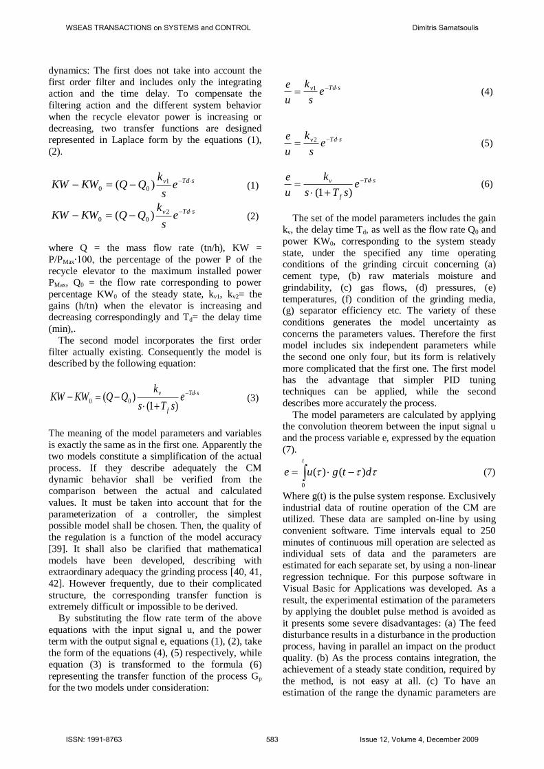
calculated variances are demonstrated in the Figures

5 and 6. As it can be observed from these figures the fitting between experimental and calculated

variances is very good.

Figure 5. χ

2 distributions for the first model.

Figure 6. χ

2 distributions for the second model.

3.2 Function between Model Parameters and

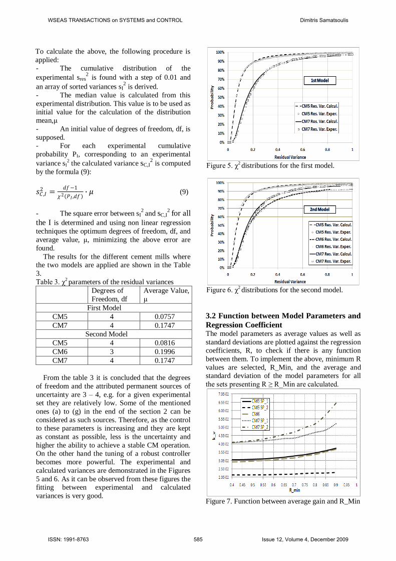
Regression Coefficient The model parameters as average values as well as

standard deviations are plotted against the regression coefficients, R, to check if there is any function

between them. To implement the above, minimum R

values are selected, R_Min, and the average and standard deviation of the model parameters for all

the sets presenting R ≥ R_Min are calculated.

Figure 7. Function between average gain and R_Min



The results of these statistics of the gain kv as

function of R_Min are depicted in the figures 7 and 8 respectively. The second model parameters are

chosen because of the larger number of experimental

sets. During the period investigated, CM5 initially

operated with a set point of the elevator power equal to 18% – SP 1 – and then with a set point equal to

26.7% - SP 2 - of the of the maximum power. The

set point of CM7 was initially equal to 28% - SP 1 - and then 30% - SP 2 - of the maximum power. CM6

set point was always the same and equal to 36.6% of

the maximum.

Figure 8. Function between standard deviation of gain and R_Min

A trend between the average gain and the R_Min can be observed from the Figure 7. As the model

regression coefficient increases, the gain increases

as well. That means that the disturbances not only

affect the model accuracy, but also cause the estimation of a lower gain. Conversely the standard

deviation of the gain is independent of the level of

R_Min. As a result for all the range of R_Min, the model uncertainty remains practically invariant as

the gain is concerning. This trend between R_Min

and gain could be explained from the natural

meaning of the gain: When a departure from the equilibrium point, Q-Q0, occurs, then after Td

minutes, this change is transferred to the recycle

elevator as kv∙(Q-Q0), passing firstly from a first order filter with a time constant Tf. A model of poor

accuracy is insufficient to predict the actual

variation of the elevator power resulting in a calculated power change lower than the actual one,

e.g. gain smaller than the actual.

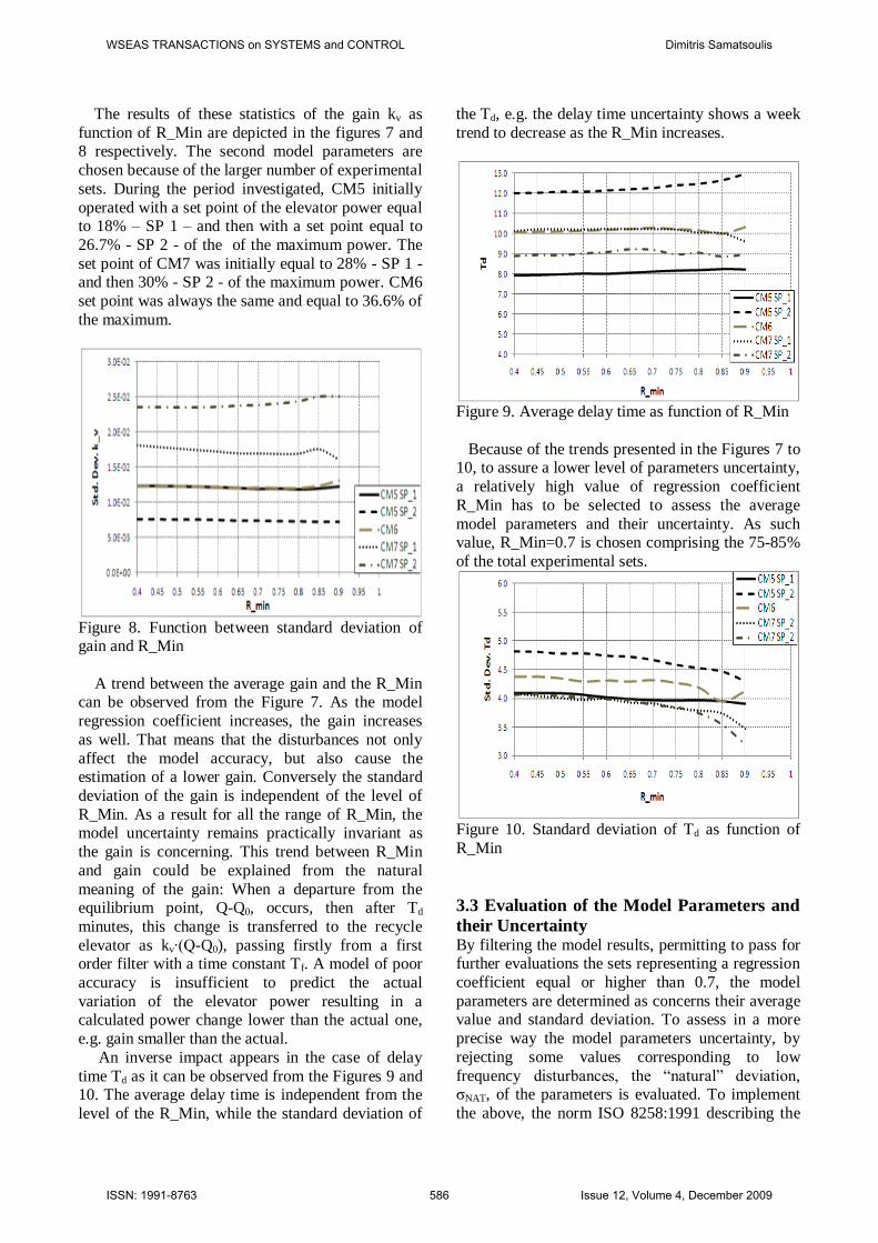
An inverse impact appears in the case of delay

time Td as it can be observed from the Figures 9 and 10. The average delay time is independent from the

level of the R_Min, while the standard deviation of

the Td, e.g. the delay time uncertainty shows a week

trend to decrease as the R_Min increases.

Figure 9. Average delay time as function of R_Min

Because of the trends presented in the Figures 7 to 10, to assure a lower level of parameters uncertainty,

a relatively high value of regression coefficient

R_Min has to be selected to assess the average

model parameters and their uncertainty. As such value, R_Min=0.7 is chosen comprising the 75-85%

of the total experimental sets.

Figure 10. Standard deviation of Td as function of

R_Min

3.3 Evaluation of the Model Parameters and

their Uncertainty By filtering the model results, permitting to pass for further evaluations the sets representing a regression

coefficient equal or higher than 0.7, the model

parameters are determined as concerns their average value and standard deviation. To assess in a more

precise way the model parameters uncertainty, by

rejecting some values corresponding to low

frequency disturbances, the ―natural‖ deviation, σNAT, of the parameters is evaluated. To implement

the above, the norm ISO 8258:1991 describing the



Sewhard control charts is utilized. To calculate this

statistic the following steps are needed: (a) Calculate the absolute range Ri between two

consecutive parameters Xi, Xi-1 and the average

range RAver, over all the ranges population, by

applying the equations (10):

𝑅𝑖 = 𝑋𝑖 − 𝑋𝑖−1 𝑅𝐴𝑣𝑒𝑟 = 𝑅𝑖

𝑁𝑖=1

𝑁 (10)

(b) Calculate the maximum range, RMax, for 99%

probability provided by the formula (11). Each

R > RMax is considered as an outlier and the values

are excluded from further calculations.

𝑅𝑀𝑎𝑥 = 3.267 ∙ 𝑅𝐴𝑣𝑒𝑟 (11)

(c) After the exclusion of all the outliers and

calculation of a final RAver, the process natural

deviation concerning the parameter under

investigation is calculated using the equation (12):

𝜎𝑁𝐴𝑇 = 0.8865 ∙ 𝑅𝐴𝑣𝑒𝑟 (12)

Table 4. First model parameters

Cement Mills

Parameters CM5 CM7

Average kv1 3.0∙10-2

4.8∙10-2

Std. Dev. kv1 1.6∙10-2

2.7∙10-2

σNAT kv1 1.5∙10-2

2.4∙10-2

%CV 49.8 55.8

Average kv2 3.2∙10-2

4.1∙10-2

Std. Dev. kv2 1.6∙10-2

2.7∙10-2

σNAT kv2 1.6∙10-2

2.1∙10-2

%CV 50.0 51.7

Average Td 10.2 13.9

Std. Dev. Td 3.2 3.8

σNAT Td 3.1 3.4

%CV 30.7 24.2

Average Q0 25.8 33.4

Std. Dev. Q0 0.9 1.4

%CV 3.5 4.1

Average KW0 17.6 24.7

Std. Dev.KW0 3.4 7.3

%CV 19.1 29.4

R_CAver 0.86 0.87

The parameters results concerning average values,

standard and natural deviations for all the cement

mills are presented in the Tables 4, 5, 6. The coefficients of variation of parameters, %CV and the

average regression coefficients, R_CAver are also

demonstrated.

Table 5. Second model parameters

Cement Mills

Parameters CM5 SP 1

CM6 CM7 SP 1

Average kv 3.3∙10-2

3.2∙10-2 4.4∙10

-2

Std. Dev. kv 1.2∙10-2

1.2∙10-2 1.7∙10

-2

σNAT kv 9.1∙10-3

1.1∙10-2 1.6∙10

-2

%CV 27.6 35.7 36.1

Average Td 8.1 10.3 10.2

Std. Dev. Td 4.0 4.3 3.9

σNAT Td 3.4 4.0 3.5

%CV 41.6 39.0 34.4

Average Q0 25.6 66.8 33.4

Std. Dev. Q0 1.8 2.1 1.2

%CV 7.2 3.2 3.7

Average KW0 17.6 36.6 26.4

Std. Dev.KW0 3.4 6.6 6.3

%CV 19.3 18.0 23.7

R_CAver 0.86 0.84 0.86

Table 6. Second model parameters

Cement Mills

Parameters CM5

SP 2

CM7

SP 2

Average kv 2.2∙10-2

4.7∙10-2

Std. Dev. kv 7.7∙10-3

2.4∙10-2

σNAT kv 6.3∙10-3

1.6∙10-2

%CV 28.7 33.4

Average Td 12.0 9.2

Std. Dev. Td 4.6 3.9

σNAT Td 4.1 3.5

%CV 34.1 38.2

Average Q0 28.3 32.2

Std. Dev. Q0 2.1 1.8

%CV 7.3 5.6

Average KW0 26.4 30.8

Std. Dev.KW0 3.8 7.8

%CV 14.4 25.4

R_CAver 0.89 0.84

In spite that the coefficients of variation are

calculated using the natural deviation as the gain and

delay time is concerning, they are very high for both models: For the first model 50-55% as to kv and 24-

31% as to Td. The coefficients of variation, %CV,

computed for the second model are 28-36% and 34-42 % as to kv and Td respectively. Especially for the

second model, the cumulative distributions of the

gain kv and delay time Td, for the three mills under consideration, are depicted in the Figures 11 and 12

respectively.



Figure 11. Cumulative distribution of kv

From these two figures the high uncertainty of

the model parameters becomes more obvious.

Figure 12. Cumulative distribution of Td

To investigate if the normal distribution is good

approximation of the gain and delay time distributions, the statistical norm ISO 2854-1976 is

applied: For each cumulative experimental

probability Pa, the corresponding normalized

distance from the average, μ, in standard deviation σ, units, given by the formula (13) is computed.

𝑧𝑎 =𝑧−𝜇

𝜎 (13)

The gain and the delay time are plotted against the variable za. The better a straight line fits the

resulting points, the higher the approximation by a

normal distribution is. The mean value of the

distribution corresponds to za=0, while the distribution standard deviation is equal to the slope.

The kv and Td curves related to each mill and set

point are depicted in the Figures 13 to 16.

Figure 13. kv as a function of the variable za – CM5, CM6

Figure 14. kv as a function of the variable za – CM7

Figure 15. Td as a function of the variable za – CM5,

CM6

From the Figures 13 to 16 it is concluded that the

dynamic parameters follow in the most cases the

normal distribution with a good approximation. Probably only the gain for CM7 and set point 2



show a relatively significant departure from the

normality.

Figure 16. Τd as a function of the variable za – CM7

Some also important conclusions can also be extracted as concerns the impact of the set point

value on the parameters uncertainty:

- The significantly larger SP 2 than SP 1 in the case of CM5 leads to a lower gain and a higher

delay time. For a higher set point, the elevator is

more loaded with material, so the same increase of the feed and of the variable Q-Q0, results in a

lower increase of the (KW-KW0)/(Q-Q0)

variable. For the same reason any change of the

feed, will appear later to the recycle elevator, resulting in an increase of the delay time. The

Niquist plots of the CM5 transfer functions for

the two set points and demonstrated in the Figure 17. The X-axis and Y-axis represent the

transfer function real and imaginary part

respectively for different frequencies ω.

- Because the difference between SP 1 and SP 2 in CM7 is small, the delay times are similar.

Other reasons shall be searched to find the

important difference in the gains.

Figure 17. Niquist plots of the CM5 transfer functions for the 2 set points

The probable covariance between the model

parameters is also investigated. As indicator of such covariance, the regression coefficient, R, between

two populations of parameters is considered. Each

parameter pair corresponds to the same experimental

set. For each cement mill and set point a table of regression coefficients is calculated and the average

R over the three CM is then found. The results are

shown in the table 7.

Table 7. Parameters regression coefficients

Td kv Q0 KW0

Td 1 -0.093 0.011 -0.008

kv 1 -0.077 0.039

Q0 1 0.184

KW0 1

From the Table 7, a positive week correlation can be

observed between Q0 and KW0: In the case the feed

is stabilized in a feed rate Q0, then as Q0 increases,

KW0 also enlarges. The power augmentation of the recycle elevator is the result of the rise of the circuit

circulating load as the feed flow rate increases. A

negative also week correlation seems to exist between Td and kv caused probably from material

accumulation inside the CM.

3.4 Impact of the Cement Composition on the

Parameters Uncertainty Except the CM7 where one cement type is

ground primarily, the two other cement mills

process mainly three types. In the following analysis the subsequent codification is used as concerns the

cement types: 1=CEM II A-L 42.5, 2=CEM IV B

(P-W) 32.5, 3=CEM II B-M (P-L) 32.5. The composition of these cements according to EN 197-

1 is given in the table 8 as to the main components.

As it can be observed from this table the three

cement types differ significantly in the clinker content and the other main components as well.

Subsequently, there is a big probability the grinding

of each one to show different dynamic, resulting in a source of uncertainty of the model parameters.

Table 8. Cement compositions

Cement Clinker Lime- stone

Pozzo- lane

Fly ash

1 80-94 16-20 - -

2 45-64 - 36-55

3 65-79 21-35 -

For the cement mills 5 and 6 and for each cement

type, the second model parameters and their



standard deviation are calculated. The percentage of

time that each mill grinds each type is also evaluated and illustrated in the Table 9.

Table 9. Percentage of time of each CEM type

CEM Type

CM5 SP 1

CM5 SP 2

CM6 CM7 SP 1

CM7 SP 2

1 8 7 34.6 100 66.4

2 61.9 37.8 18.5

3 30.1 55.2 46.9 33.6

From the table 9 it is concluded that CM5 grinds

primarily CEM IV B (P-W) and CEM II B-M (P-L)

but also some significant quantities of CEM II A-L. On the contrary CM6 grinds mainly CEM II A-L

and CEM II B-M (P-L) and not negligible quantities

of CEM IV B (P-W) too. The gains and time delay results for all cases investigated are presented in the

Table 10. These values are compared with the ones

shown in the Tables 5, 6.

Table 10. Average values of the parameters

Type CM5 SP 1 CM6

Average Std.Dev Average Std.Dev.

kv×102

All 3.3 1.2 3.2 1.2

1 3.5 1.5 3.0 1.1

2 3.0 1.0 3.0 1.2

3 3.7 1.2 3.3 1.2

Td

All 8.1 4.0 10.3 4.3

1 10.2 3.4 11.0 3.9

2 7.5 3.9 10.5 4.6

3 8.4 3.8 9.0 4.1

CM5 SP 2 CM7 SP 2


kv×102

All 2.2 0.8 4.7 2.4

1 2.1 0.6 5.1 2.6

2 2.3 0.8

3 2.1 0.7 4.4 2.1

Td


All 12 4.6 9.2 3.9

1 13.7 5.0 8.9 3.7

2 10.1 4.8

3 13.7 4.2 9.7 3.7

The Td results are also demonstrated in the Figure

18 where the average delay time per cement type for

each CM and SP is also computed and compared. The gain kv is higher in the case of the CEM II B-M

(P-L) cement in comparison with the two other

types, which means that for an input u an elevated

output e is derived. CEM IV presents in any case the lower gain, because the most portion of the fly ash

does not pass from the mill as it is fed directly to the

dynamic separator. For this also reason the delay

time of the CEM IV is the lower among the three cement types. The CEM A-L because of the elevated

clinker content presents the higher delay time as it is

the cement of the lower grindability. The standard deviations of the gains for each cement type do not

differ noticeably from the total one. On the other

hand the Td standard deviations are in general lower for each cement type than the overall one.

Figure 18. Td for different cement types

The transfer function plots for the different mills

and the main cement types ground to each one are

depicted in the Figure 19. The significant difference of the transfer functions for the various cement types

in the same CM is obvious from this figure.

Figure 19. Niquist plots of the different cement

types transfer functions

As a conclusion the grinding of different cement types to the same mill, has a severe impact on the

model uncertainty, as in general the parameters for



each type differ significantly. The above generates

problems in the tuning of a controller: If the controller is adjusted according to the average

parameters, then this selection is not generally

optimal for each cement type. If the tuning is based

on the dynamic of one cement type, probably the regulation is not good for the other types.

Apparently a fine solution is to dedicate as much as

possible each cement mill for one cement type.

3.5 Impact of the Ball Charge Condition on

the Parameters Uncertainty It well known that the grinding media charge as total load and as composition as well, has a very strong

effect on the CM productivity and product quality. A

good indication of the current ball volume is the CM

absorbed power, as the two variables are linearly related: For each specific mill, the process engineers

have knowledge how many KW absorbs one ton of

balls and they use this value to add balls in the CM, when the absorbed power drops.

To investigate the impact of the ball charge on the

model parameters the following procedure is designed and performed:

- For each CM and cement type the set of data

including the dynamic parameters is sorted

according to the absorbed power. - The data are separated in two subsets of higher

and lower power. For the case of CM5 SP 2 the

power difference between the two sets was not significant, less than 30 KW. So these data were

excluded from further processing

- The average values of model parameters and

power are calculated for each subset. Five cases are processed in total.

The results are presented in the Table 11.

Table 11. Impact of the CM power on the model

parameters

Td kv×102 Cem. Type Mill KW

CM6

11.6 3.2 1 1824

12.3 2.9 1 1901

8.4 3.6 3 1817

9.5 3.1 3 1889

CM5 SP 1

7.0 3.1 2 799

7.7 2.9 2 854

9.4 3.2 3 815

7.9 4.2 3 874

CM7

8.9 5.1 1 951

10.2 4.4 1 1157

In four out of the five cases studied, as the CM

power increases, the gain drops and the delay time increases. Consequently the condition of the ball

charge is a strong factor affecting the total model

uncertainty. The physical meaning of these results is

the following: As the ball charge is new and high, the mill productivity is higher, for given quality

targets. So an increase of the variable Q-Q0, causes

less return, because the CM grinds finer resulting in lower KW-KW0, comparing with the low power

case. For this reason the gain is lower in the case of

the high mill power. For fresh grinding media charge and high power, because of the better

grinding, the increase of the feed Q, causes a slower

increase of the return flow rate in comparison with

the low power condition. Therefore the increase of the elevator power is delayed resulting in an

increase of the model delay time.

4 Applied Techniques of PID Tuning It is critical in control system design and tuning to

assure the stability and performance of the closed

loop in the case that a mismatch between accepted and actual model occurs, i.e. to guarantee

robustness.

The feedback loop of the system to be controlled is given in the simplest possible form in the Figure 20.

Figure 20. Feedback control loop

The system loop is composed from the grinding

process Gp and the controller Gc. The grinding

process is influenced by the controller via the variable u that is the mill feed. With the fresh feed

also enter in the mill its characteristics as

composition, grindability, temperature. The above represent a part of the disturbance d. Another

portion of the disturbance represents the gas flow

rate and its temperature. A third also portion can

represent the mass flow of the separator return and the corresponding physical and chemical

characteristics. For example a step change to the

separator speed or to the gases passed from the separator, causes a change to the return flow rate



and its characteristics and consequently a further

disturbance to the grinding operation. Apparently such adjustments sometimes are desirable for quality

purposes, depending of the final product measured

characteristics. These short term disturbances affect

the process model accuracy and they have a certain impact on the model regression coefficient. As

process output x, the recycle elevator power is

considered that shall be controlled. Control is based on the measured signal y, where the measurements

are corrupted by measurement noise n. Information

about the process variable x is thus distorted by the measurement noise. To smooth the variable x, a first

order filter with time constant Tf is added in the

three CM under consideration by paying a relatively

delayed response of the system. This time constant is selected notably less that the system delay time

after some first evaluations of this variable and by

experience as well. The controller is a system with two inputs: The measured elevator power y and the

elevator set point yst. The difference yst – y provides

the signal error e. The controller transfer functions

Gc is given by the typical form (14) according to

Angstrom and Hagglund [10]. The variables kp, ki,

kd represent the proportional, integral and

differential coefficients of the controller correspondingly.

sks

kk

e

ud

ip (14)

The same equation expressed in time difference form, to be possible to be passed in the CM

operating system, is expressed by the equations (15),

(16) where Δt is the sampling period in seconds:

𝑒𝑛 = 𝑦𝑠𝑡 − 𝑦 (15)

𝑢𝑛 = 𝑢𝑛−1 + 𝑘𝑝 ∙ 𝑒𝑛 − 𝑒𝑛−1 +Δt

60∙ 𝑘𝑖 ∙ 𝑒𝑛 +

𝑘𝑑 ∙1

Δ𝑡∙ 𝑒𝑛 + 𝑒𝑛−2 − 2 ∙ 𝑒𝑛−1 (16)

Probably the best criterion of performance is the sensitivity function determined by the Laplace

equation (17):

𝑆 =1

1+𝐺𝑐𝐺𝑝 (17)

An additional function to characterize the

performance is also the complementary sensitivity function provided by the equation (18):

𝑇 =𝐺𝑐𝐺𝑝

1+𝐺𝑐𝐺𝑝 (18)

Apparently S+T=1. The function S tells how the closed loop properties are influenced by small

variations in the process [14]. The maximum

sensitivities represented by the equation (19) can be used as robustness measures.

𝑀𝑠 = 𝑀𝑎𝑥 𝑆 𝑖𝜔 𝑀𝑡 = 𝑀𝑎𝑥 𝑇 𝑖𝜔 (19)

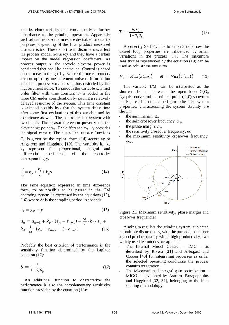
The variable 1/Ms can be interpreted as the

shortest distance between the open loop GcGp

Nyquist curve and the critical point (-1,0) shown in

the Figure 21. In the same figure other also system properties, characterizing the system stability are

shown:

- the gain margin, gm - the gain crossover frequency, ωgc

- the phase margin, φm

- the sensitivity crossover frequency, ωsc - the maximum sensitivity crossover frequency,

ωmc.

Figure 21. Maximum sensitivity, phase margin and

crossover frequencies

Aiming to regulate the grinding system, subjected

in multiple disturbances, with the purpose to achieve a good product quality with a high productivity, two

widely used techniques are applied:

- The Internal Model Control – IMC – as

described by Rivera [21] and Arbogast and Cooper [43] for integrating processes as under

the selected operating conditions the process

contains integration. - The M-constrained integral gain optimization –

MIGO – developed by Astrom, Panagopoulos

and Hagglund [32, 34], belonging to the loop shaping methodology.



The performance of the implemented controllers

is assessed in the following way: - By building the convenient software, the daily

CM data are loaded.

- The period of sampling is one minute. Therefore

in 24 hours, up to 1440 points are loaded. The time period that the CM is stopped is excluded

easily by the software, taking into account the

mill motor power. - Using the software, an effort is made to detect

automatically the period that the CM runs in

automatic mode, as when the CM starts to operate and up to be the circuit loaded, the

manual mode is necessary.

- For a given set point of the power, KWsp, the

automatic mode operation performance is

evaluated via the Integral of Absolute Error –

IAE – computed by the Equation (20).

dtKWtKWt

IAE

t

sp

0

00

)(1

(20)

4.1 Implementation of the IMC technique The IMC tuning is applied to regulate the recycle

elevator in two out of the three CM: CM5 and CM7. Before this technique to be selected, the PID

parameters were adjusted by trial and error and the

operation was in general satisfactory. The three controller parameters are calculated using the

system of equations (21):

Derivpd

Int

p

i

dC

dCdDerivdCInt

C

dC

v

PdC

TkkT

kk

TT

TTTTTTT

TdT

TT

kkTT

2

25.02

5.0

2110

2

2

(21)

Where Tc is a time parameter (min) connected

with the time constant of the feedback control loop and consists a design parameter, determined by the

value of the tuning parameter α. A value of

α=1corresponds to typical design, while a value equal to 5 to conservative one. As concerns the

maximum sensitivity Ms, a predetermined constraint

is not put implicitly, but it is computed after the calculation of the open loop transfer function, at it

depends on the value of the α parameter. For the

calculation of the design parameter Tc a value α=1

has been considered for CM5, while α=0.7 for CM7, to provide a similar Tc value 31 to 32 min. The PID

tuning was made after a sufficient number of data

was collected for a period of at least 20 days. Then the PID with the tuned coefficients was put in

operation. The results are depicted in the Table 12.

For comparison reasons the PID parameters derived

with trial and error are shown in the Table 13. Based also on the experience, minimum and maximum

permissible feed flow rates are added to the

controllers.

Table 12. PID parameters after IMC application

Elevator

ascent

Elevator

descent

Elevator

ascent

Elevator

descent

CM5 CM7

kp 1.43 2.15 1.31 1.43 ki 0.03 0.03 0.019 0.021 kd 5.2 7.0 7.7 8.4

Table 13. PID parameters found with trial and error

Elevator

ascent

Elevator

descent

Elevator

ascent

Elevator

descent

CM5 CM7

kp 0.6 0.6 0.6 0.6 ki 0.03 0.04 0.03 0.04 kd 7.0 8.0 7.0 8.0

The performance comparison between the two sets

of PID parameters for each CM is executed using the daily IAE.

Figure 22. IAE comparison for CM5.

Furthermore, using the equations (10)-(12) the

outlying IAE are detected and excluded and a

control chart for each CM is constructed according to ISO 8258:1991. Subsequently the average IAE

and the portion of outliers comparing to the total

population for each parameters set is found. The

above result in a further comparison between the two parameter sets for each mill. The daily IAE are

illustrated in the Figures 22 and 23 for CM5 and

CM7 respectively. In the same figures the average IAE and the upper and low 3σ limits after the



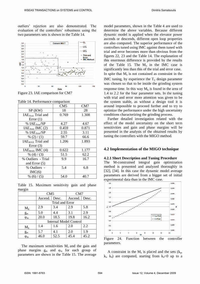
outliers’ rejection are also demonstrated. The

evaluation of the controllers’ robustness using the two parameters sets is shown in the Table 14.

Figure 23. IAE comparison for CM7

Table 14. Performance comparison

CM5 CM7

SP (KW) 18 28

IAEAver Trial and

Error (1)

0.769 1.308

% IAEAver/SP 4.27 4.67

IAEAver IMC (2) 0.459 0.871

% IAEAver/SP 2.55 3.11

% (2) / (1) 59.7 66.6

IAEMAX Trial and

Error (3)

1.206 1.893

IAEMAX IMC (4) 0.622 1.177

% (4) / (3) 51.5 62.2

% Outliers - Trial

and Error (5)

9.9 16.7

% Outliers -

IMC(6)

5.4 6.8

% (6) / (5) 54.0 40.7

Table 15. Maximum sensitivity gain and phase

margin

CM5 CM7

Ascend. Desc. Ascend. Desc.

Trial and Error

Ms 2.9 3.4 2.9 5.8

gm 5.0 4.4 3.1 2.9

φm 20.0 18.5 19.8 16.2

Internal Model Control

Ms 1.4 1.6 2.0 2.2

gm 5.7 4.1 2.0 1.9

φm 46.0 52.5 45.4 45.2

The maximum sensitivities Ms and the gain and phase margins gm and φm for each group of

parameters are shown in the Table 15. The average

model parameters, shown in the Table 4 are used to

determine the above variables. Because different dynamic model is applied when the elevator power

ascends or descends, different open loop properties

are also computed. The superior performance of the

controllers tuned using IMC against them tuned with trial and error becomes more than obvious from the

figures 22, 23 and the Table 14. The explanation of

this enormous difference is provided by the results

of the Table 15. The Ms in the IMC case is

significantly less than this of the trial and error case.

In spite that Ms is not contained as constraint in the

IMC tuning, by experience the Tc design parameter

was chosen so that to be inside the grinding system

response time. In this way Ms is found in the area of

1.4 to 2.2 for the four parameter sets. In the tuning

with trial and error more attention was given to be the system stable, as without a design tool it is

around impossible to proceed further and to try to

optimize the performance under the high uncertainty conditions characterizing the grinding process.

Further detailed investigation related with the

effect of the model uncertainty on the short term

sensitivities and gain and phase margins will be presented in the analysis of the obtained results by

tuning the controllers with the MIGO method.

4.2 Implementation of the MIGO technique

4.2.1 Short Description and Tuning Procedure

The M-constrained integral gain optimization method is presented and analyzed thoroughly in

[32], [34]. In this case the dynamic model average

parameters are derived from a bigger set of initial

experimental data than in the IMC case.

Figure 24. Function between the controller

parameters.

A constraint in the Ms is placed and the sets (kp,

ki, kd) are computed, starting from kd=0 up to a



maximum value of kd satisfying the Ms constraint.

When kd is maximum, the same occurs also for kp,

ki. An example of the function between the three

PID coefficients as kd varies from 0 to a maximum

value is provided in the Figure 24. The open loop

transfer function is restricted to have Ms ≤ 1.5. The

dynamic parameters of CM5 for SP 2 are

considered. From this figure it is concluded that a change of kd from 0 to 12 causes an 80% increase of

kp while the ki is augmented by three times. In

parallel the constraint of Ms is always fulfilled. The

open loop Nyquist functions for kd=0, 3, 7, 10 are shown in the Figure 25.

Figure 25. Niquist plots for Ms=1.5 and different kp

Consequently the applied loop shaping technique

possesses the great benefit to provide for the same maximum sensitivity a set of parameters satisfying

this constraint. From this set a corresponding set of

gain and phase margins can be determined. By

varying kd from 0 to 11, the range of these margins are obtained and illustrated in the Figure 26.

Figure 26. Gain and phase margins as function of kd

As the differential part increases, both gain and

phase margins are decreasing. Therefore the kd and

the corresponding coefficients set shall be selected

with one of the following ways:

(a) To take a kd near to the middle of the range.

(b) To decide according to a designed or

predetermined gain or phase margin. (c) To determine the kd providing the minimum

IAE using some kind of simulation of the real

operation.

4.2.2 Controllers Parameterization and IAE

results In the level of development of this research, the set

of parameters is selected using a kd in the middle of

the acceptable range for a predetermined Ms. The

parameter values for the different CM and recycle elevator set points are provided in the Table 16.

Table 16. PID coefficients tuned with MIGO

CM5 SP 1

CM5 SP 2

CM7 SP 1

CM7 SP 2

kp 1.61 1.90 1.07 1.07

ki 0.043 0.027 0.025 0.025

kd 7.0 7.0 7.0 7.0

CM6

kp 1.3

ki 0.03

kd 7.0

As in the case of IMC, the tuning with MIGO was

based on the existing dynamic data when this

procedure was performed and not on the full data set deriving the parameters of the Tables 5 and 6. The

daily IAE for the three CM and the different set

points are depicted in the Figures 27, 28, 29.

Figure 27. %CV of IAE for CM5

To compare better for the various set points, but

also between cement mills results, the IAE are

expressed as %CV of IAE, by the formula𝐼𝐴𝐸

𝑆𝑃∙ 100.

In the same figures the %CV of IAE by applying trial and error and IMC tuning are also shown. As



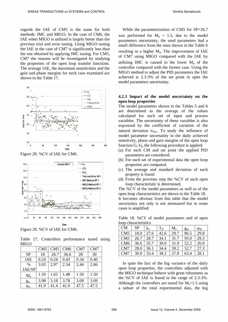
regards the IAE of CM5 is the same for both

methods: IMC and MIGO. In the case of CM6, the IAE when MIGO is utilized is largely better than the

previous trial and error tuning. Using MIGO tuning

the IAE in the case of CM7 is significantly less than

the one obtained by applying IMC tuning. For CM5, CM7 the reasons will be investigated by studying

the properties of the open loop transfer functions.

The average IAE, the maximum sensitivities and the gain and phase margins for each case examined are

shown in the Table 17.

Figure 28. %CV of IAE for CM6.

Figure 29. %CV of IAE for CM6.

Table 17. Controllers performance tuned using MIGO

CM5 CM5 CM6 CM7 CM7

SP 18 26.7 36.6 28 30

IAE 0.24 0.24 0.43 0.34 0.40

%

IAE/SP

3.03 2.97 2.34 2.44 2.66

Ms 1.50 1.65 1.48 1.50 1.50

gm 3.98 3.18 3.78 3.09 3.09

φm 41.9 41.4 41.9 47.5 47.5

While the parameterization of CM5 for SP=26.7

was performed for Ms = 1.5, due to the model

parameters uncertainty, the used parameters had a small difference from the ones shown in the Table 6

resulting in a higher Ms. The improvement of IAE

of CM7 using MIGO compared with the IAE by

utilizing IMC is caused to the lower Ms of the

controller compared with the former case. Using the

MIGO method to adjust the PID parameters the IAE achieved is 2.3-3% of the set point in spite the

model parameters uncertainty.

4.2.3 Impact of the model uncertainty on the

open loop properties

The model parameters shown in the Tables 5 and 6 are determined as the average of the values

calculated for each set of input and process

variables. The uncertainty of these variables is also expressed by the coefficient of variation of the

natural deviation σNat. To study the influence of

model parameter uncertainty in the daily achieved sensitivity, phase and gain margins of the open loop

function Gc∙Gp the following procedure is applied:

(a) For each CM and set point the applied PID

parameters are considered. (b) For each set of experimental data the open loop

properties are computed.

(c) The average and standard deviation of each property is found

(d) From the previous step the %CV of each open

loop characteristic is determined. The %CV of the model parameters as well as of the

open loop characteristics are shown in the Table 18.

It becomes obvious from this table that the model

uncertainty not only is not attenuated but in some cases is amplified.

Table 18. %CV of model parameters and of open loop characteristics

CM SP kv Td Ms gm φm

CM5 18.0 27.6 41.6 29.7 86.5 29.8

CM5 26.7 28.7 34.1 31.7 93.0 29.3

CM6 36.6 35.7 39.0 31.9 52.2 26.9

CM7 28.0 36.1 34.4 39.2 52.7 27.3

CM7 30.0 33.4 38.2 27.8 63.4 28.1

In spite the fact of the big variance of the daily

open loop properties, the controllers adjusted with

the MIGO technique behave with great robustness as the %CV of IAE is found in the range of 2.3-3%.

Although the controllers are tuned for Ms=1.5 using

a subset of the total experimental data, the big



variance of the daily Ms derives an average Ms

usually a few higher from the designed one. An

example of maximum sensitivity distribution for the results of CM5 and both set points is presented in

the Figure 30.

Figure 30. Ms cumulative distribution for CM5

As it is mentioned earlier MIGO provides a full

group of (kp, ki, kd) parameters ranging from kd=0 to

a maximum value fulfilling the constraint of Ms as

to the open loop transfer function. If no other

constraint is set, then kd is the design parameter.

Based on actual data sets and for a predefined Ms,

an investigation is carried out concerning the impact

of the kd value on the data set average Ms and its

standard deviation.

Figure 31. Average and standard deviation of Ms as

function of kd.

The dynamic parameters of CM5 SP1 and CM5

SP2 are considered. Using them the PID coefficients

are computed for Ms = 1.5 and an array of (kp, ki, kd)

is obtained. Then for the dynamic parameters of

each data set the individual Ms are found and their

average and standard deviation as well. The results

are depicted in the Figure 31.

As kd increases, the average Ms and its standard

deviation grow too. After a certain kd value, average

Ms deviates notably from the designed one. To avoid

this undesirable phenomenon, probably it is better to

design with a lower Ms, to be able to tune the

parameters with a higher kd.

To examine the effect of the predetermined Ms

according to the design on the population average

Ms and its variance, the following procedure is

executed:

(a) The CM5 SP 2 data sets are considered and the

individual dynamic of its set.

(b) Two values of kd are chosen: kd = 2 and kd =8.

(c) The Ms constraint is getting values in the

interval [1.5, 2.0] for SP 1 and [1.3, 2.3] for SP2

(d) The population average and a maximum Ms, 80

are computed. In the interval [0, Ms, 80] the 80%

of the Ms population is contained.


function of the Ms constraint for CM5 SP 1.


function of the Ms constraint for CM5 SP 2. The results are shown in the Figures 32 and 33 for

SP 1 and SP 2 respectively. Similar to these figures



are also obtained for the two other CM. From these

figures the following conclusions can be extracted:

- For any designed Ms constraint the average of

the actual population is higher than the

designed.

- The difference between actual average and

designed Ms is amplified as the designed

constraint increases.

- As the constrain increases the critical Ms80 also

is considerably growing.

- For the grinding closed circuits under

investigation, a robust design shall have as

maximum Ms limitation a value of 1.6, in order

to permit a maximum actual average Ms of 2.0.

4.2.4 MIGO design for different cement types

As it is in detail described in section 3.4, different

cement types ground in the same CM and for the same elevator set point, present diverse dynamic

behavior resulting in different dynamic parameters

depicted in the Table 10. Consequently this is one of the causes of the model parameters uncertainty if the

various cement types are not taken into account. To

evaluate the effect of those dynamics on the open loop transfer function the subsequent procedure is

built.

(a) For the average model parameters shown in the

Tables 5, 6 the PID parameters are adjusted for

an Ms=1.5 and kd=7.

(b) For these dynamic parameters and PID coefficients, the open loop transfer function is

found.

(c) For the same PID coefficients and the

parameters shown in the Table 10, the open loop transfer function is determined for the main

cement types ground to each CM.

(d) The resulting transfer functions are compared. The derived parameters and the open loop

properties are presented in the Table 19. It is easily

concluded from this table that the open loop of

cements containing more clinker – according to the Table 8 – and becoming harder to be ground, present

elevated Ms, and lower gm and φm. Therefore by

applying PID controllers tuned using the average model parameters, the easiness to regulate depends

on the clinker content for the given cement types.

The transfer functions obtained for CM6 are illustrated in the Figure 34 and it becomes clearer

that the open loop transfer functions and

consequently the typical controller performance

differs for the various cement types. Subsequently, it should be examined if there are PID coefficients

applied to the average dynamic of each cement type

deriving controllers of the same performance as the one obtained with the average model parameters.

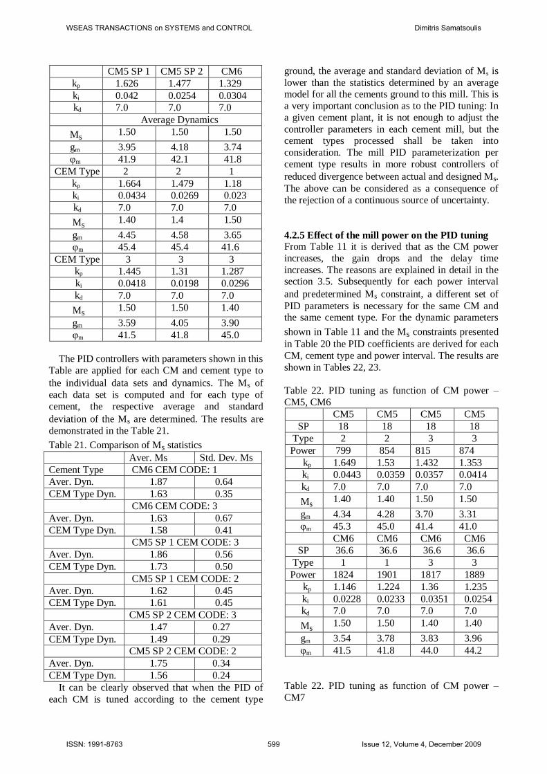
Table 19. PID coefficients and open loop

characteristics for average model

CM5

SP 1

CM5

SP 2

CM6

kp 1.626 1.477 1.329

ki 0.042 0.0254 0.0304

kd 7.0 7.0 7.0

Average Dynamics

Ms 1.50 1.50 1.50

gm 3.95 4.18 3.74

φm 41.9 42.1 41.8

CEM Type 2 2 1

Ms 1.40 1.38 1.70

gm 4.50 4.57 3.26

φm 45.4 46.7 36.1

CEM Type 3 3 3

Ms 1.57 1.65 1.42

gm 3.25 3.72 3.84

φm 41.7 37.6 44.7

Figure 34. Nyquist plots for CM6 and different cement types.

To investigate the above, MIGO is applied using the model of each cement type for each CM. If for a

cement type and according to Table 19 Ms > 1.5,

then the constraints Ms=1.5 and kd=7 are considered.

Otherwise if according to Table 19 Ms<1.5, this

value has been taken as constraint. The kd value is

chosen to provide the same gain margin as the one

depicted in the former Table for the mentioned

cement type. The results are presented in the Table 20.

Table 20. PID coefficients and open loop

characteristics for each cement type model



CM5 SP 1 CM5 SP 2 CM6

kp 1.626 1.477 1.329

ki 0.042 0.0254 0.0304

kd 7.0 7.0 7.0

Average Dynamics

Ms 1.50 1.50 1.50

gm 3.95 4.18 3.74

φm 41.9 42.1 41.8

CEM Type 2 2 1

kp 1.664 1.479 1.18

ki 0.0434 0.0269 0.023

kd 7.0 7.0 7.0

Ms 1.40 1.4 1.50

gm 4.45 4.58 3.65

φm 45.4 45.4 41.6

CEM Type 3 3 3

kp 1.445 1.31 1.287

ki 0.0418 0.0198 0.0296

kd 7.0 7.0 7.0

Ms 1.50 1.50 1.40

gm 3.59 4.05 3.90

φm 41.5 41.8 45.0

The PID controllers with parameters shown in this

Table are applied for each CM and cement type to

the individual data sets and dynamics. The Ms of

each data set is computed and for each type of

cement, the respective average and standard

deviation of the Ms are determined. The results are

demonstrated in the Table 21.

Table 21. Comparison of Ms statistics

Aver. Ms Std. Dev. Ms

Cement Type CM6 CEM CODE: 1

Aver. Dyn. 1.87 0.64

CEM Type Dyn. 1.63 0.35

CM6 CEM CODE: 3

Aver. Dyn. 1.63 0.67


CM5 SP 1 CEM CODE: 3

Aver. Dyn. 1.86 0.56



Aver. Dyn. 1.62 0.45



Aver. Dyn. 1.47 0.27



Aver. Dyn. 1.75 0.34


It can be clearly observed that when the PID of

each CM is tuned according to the cement type

ground, the average and standard deviation of Ms is

lower than the statistics determined by an average model for all the cements ground to this mill. This is

a very important conclusion as to the PID tuning: In

a given cement plant, it is not enough to adjust the

controller parameters in each cement mill, but the cement types processed shall be taken into

consideration. The mill PID parameterization per

cement type results in more robust controllers of

reduced divergence between actual and designed Ms.

The above can be considered as a consequence of

the rejection of a continuous source of uncertainty.

4.2.5 Effect of the mill power on the PID tuning From Table 11 it is derived that as the CM power

increases, the gain drops and the delay time

increases. The reasons are explained in detail in the section 3.5. Subsequently for each power interval

and predetermined Ms constraint, a different set of

PID parameters is necessary for the same CM and the same cement type. For the dynamic parameters

shown in Table 11 and the Ms constraints presented

in Table 20 the PID coefficients are derived for each

CM, cement type and power interval. The results are

shown in Tables 22, 23.

Table 22. PID tuning as function of CM power –

CM5, CM6

CM5 CM5 CM5 CM5

SP 18 18 18 18

Type 2 2 3 3

Power 799 854 815 874

kp 1.649 1.53 1.432 1.353

ki 0.0443 0.0359 0.0357 0.0414

kd 7.0 7.0 7.0 7.0

Ms 1.40 1.40 1.50 1.50

gm 4.34 4.28 3.70 3.31

φm 45.3 45.0 41.4 41.0

CM6 CM6 CM6 CM6

SP 36.6 36.6 36.6 36.6

Type 1 1 3 3

Power 1824 1901 1817 1889

kp 1.146 1.224 1.36 1.235

ki 0.0228 0.0233 0.0351 0.0254

kd 7.0 7.0 7.0 7.0

Ms 1.50 1.50 1.40 1.40

gm 3.54 3.78 3.83 3.96

φm 41.5 41.8 44.0 44.2

Table 22. PID tuning as function of CM power –

CM7



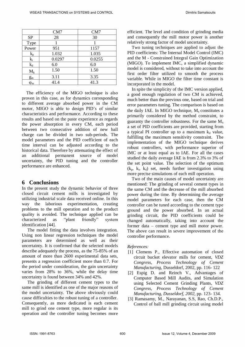
CM7 CM7

SP 28 30

Type 1 1

Power 951 1157

kp 1.032 1.035

ki 0.0297 0.0255

kd 6.0 6.0

Ms 1.50 1.50

gm 3.11 3.35

φm 41.4 41.3

The efficiency of the MIGO technique is also

proven in this case, as for dynamics corresponding to different average absorbed power in the CM

motor, MIGO is able to design PID’s of similar

characteristics and performance. According to these

results and based on the paste experience as regards the power absorption in every CM, each period

between two consecutive addition of new ball

charge can be divided in two sub-periods. The model parameters and the PID coefficient of each

time interval can be adjusted according to the

historical data. Therefore by attenuating the effect of an additional permanent source of model

uncertainty, the PID tuning and the controller

performance are enhanced.

6 Conclusions In the present study the dynamic behavior of three

closed circuit cement mills is investigated by utilizing industrial scale data received online. In this

way the laborious experimentation, creating

problems to the mill operation and to the product

quality is avoided. The technique applied can be characterized as ―plant friendly‖ system

identification [44].

The model fitting the data involves integration. Using non linear regression techniques the model

parameters are determined as well as their

uncertainty. It is confirmed that the selected models

describe adequately the process, as the 75-85% of an amount of more than 2600 experimental data sets,

presents a regression coefficient more than 0.7. For

the period under consideration, the gain uncertainty varies from 28% to 36%, while the delay time

uncertainty is found between 34% and 42%.

The grinding of different cement types to the same mill is identified as one of the major reasons of

the model uncertainty. The above obviously could

cause difficulties to the robust tuning of a controller.

Consequently, as more dedicated is each cement mill to grind one cement type, more regular is its

operation and the controller tuning becomes more

efficient. The level and condition of grinding media

and consequently the mill motor power is another relatively strong factor of model uncertainty.

Two tuning techniques are applied to adjust the

PID coefficients: The Internal Model Control (IMC)

and the M - Constrained Integral Gain Optimization (MIGO). To implement IMC, a simplified dynamic

model is considered, without to take into account the

first order filter utilized to smooth the process variable. While in MIGO the filter time constant is

incorporated in the model.

In spite the simplicity of the IMC version applied, a good enough regulation of two CM is achieved,

much better than the previous one, based on trial and

error parameters tuning. The comparison is based on

the daily IAE. In MIGO technique, Ms constitutes a

primarily considered by the method constraint, to

guaranty the controller robustness. For the same Ms

a set of PID coefficients are provided, starting from

a typical PI controller up to a maximum kd value,

fulfilling the maximum sensitivity constraint. The implementation of the MIGO technique derives

robust controllers, with performance superior of

IMC or at least equal as to IAE. For all the cases studied the daily average IAE is from 2.3% to 3% of

the set point value. The selection of the optimum

(kp, ki, kd) set, needs further investigation using

more precise simulations of each mill operation. Two of the main causes of model uncertainty are

mentioned: The grinding of several cement types in

the same CM and the decrease of the mill absorbed power during the time. By determining the average

model parameters for each case, then the CM

controller can be tuned according to the cement type

ground and the power absorbed. In an actual grinding circuit, the PID coefficients could be

changed automatically, taking into account the

former data – cement type and mill motor power. The above can result in severe improvement of the

controller performance.

References:

[1] Clemens P., Effective automation of closed

circuit bucket elevator mills for cement, VDZ

Congress, Process Technology of Cement Manufacturing, Dusseldorf, 2002, pp. 116- 122

[2] Espig D. and Reinch V., Advantages of

Computer Based Mill Audits, and Simulation using Selected Cement Grinding Plants, VDZ

Congress, Process Technology of Cement

Manufacturing, Dusseldorf, 2002, pp. 123- 134. [3] Ramasamy, M., Narayanan, S.S, Rao, Ch.D.P.,

Control of ball mill grinding circuit using model



predictive control scheme, Journal of Process

Control, 2005, pp. 273-283. [4] Chen, X., Li, Q., Fei, S., Constrained model

predictive control in ball mill grinding process,

Powder Technology, Vol. 186, 2008, pp. 31-39.

[5] Efe, M.O., Kaynak, O., Multivariable Nonlinear Model Reference Control of Cement Mills, 15th

Triennial World Congress, Barcelona, 2002.

[6] Chai, T.Y., Yue, H., Multivariable Intelligent Decoupling Control System and its Application

Acta Automatica Sinica., Vol. 31, 2005, pp. 123-

131 [7] Dagci, O.H., Efe, M.O., Kaynak, O., A

Nonlinear Learning Control Approach For a

Cement Milling Process, Proceedings of the

2001 IEEE International Conference on Control Applications, Mexico City, 2001, pp 498-503.

[8] Chen, X., Li, S., Zhai, J., Li, Q., Expert system

based adaptive dynamic matrix control for ball mill grinding circuit, Expert Systems with

Applications: An International Journal, Vol. 36,

2009, pp. 716-723. [9] Qin, S.J., Badwell, T.H., A survey of industrial

model predictive control technology, Control

Engineering Practice, Vol. 11, 2003, pp. 733-

764 [10] Astrom, K., Hagglund, T., Advanced PID

Control, Research Triangle Park:

Instrumentation, Systems and Automatic Society, 2006.

[11] Ender, D., Process Control Performance: Not

as good as you think, Control Engineering, Vol.

40, 1993, pp.180-190 [12] Gao, Z., Scaling and bandwidth -

parameterization based controller tuning,

Proceedings of the American Control Conference, Vol. 6, 2003, pp. 4989-4996.

[13] Volosencu, C., Pseudo-Equivalence of Fuzzy

PID Controllers, WSEAS Transactions on Systems and Control, Vol. 4, 2009, pp. 163-176.

[14] Astrom. K.J., Model Uncertainty and Robust

Control, Lecture Notes on Iterative Identification

and Control Design, Lund University, 2000, pp. 63–100.

[15] Astrom, K.J., Hagglund, T., The future of PID

control, Control Engineering Practice, Vol. 9, 2001, pp. 1163–1175.

[16] Ziegler, J.G., Nichols, N.B., Optimum settings

for automatic controllers, Transactions ASME, Vol. 64, 1942, pp. 759–768.

[17] Luyben, W. L., Simple method for tuning of

SISO controllers in multivariable systems.

Industrial Engineering Chemistry Process Design Development, Vol. 25, 1986, pp. 654-

663.

[18] Garcia, C.E., Morari, M., Internal Model

Control-1. A unifying review and some new results, Ind. Eng. Chem. Process Des. & Dev.,

Vol. 21, 1982, pp.308-323.

[19] Garcia, C.E., Morari M., Internal Model

Control-2. Design procedure for multivariable systems, Ind. Eng. Chem. Process Des. & Dev.,

Vol. 24, 1985, pp.472-484.

[20] Garcia, C.E., Morari, M., Internal Model Control-3. Multivariable control law

computation and tuning guidelines, Ind. Eng.

Chem. Process Des. & Dev., Vol. 24, 1985, pp.484-494

[21] Rivera, D.E., Morari, M., Skogestad, S.,

Internal Model Control 4. PID Controller

Design, Ind. Eng. Chem. Process Des. & Dev. Vol. 25, 1986, pp. 252-265

[22] Morari, M. Zafiriou, E., Robust Process

Control, Prentice Hall, 1989. [23] Yamada, K., Modified Internal Model Control

for unstable systems, Proceedings of the 7th

Mediterranean Conference on Control and Automation (MED99), Haifa, Israel, 1999, pp.

293-302.

[24] Cooper, D. J., Practical process control.

Control Station, Inc., 2004. [25] Skogestad, S., Tuning for Smooth PID Control

with Acceptable Disturbance Rejection, Ind.

Eng. Chem. Res., Vol. 45, 2006, pp. 7817-7822. [26] Skogestad, S., Tuning for Smooth PID Control

with Acceptable Disturbance Rejection, Ind.

Eng. Chem. Res., Vol. 45, 2006, pp. 7817-7822.

[27] McFarlane, D., Glover, K., A loop shaping design procedure using H∞ synthesis, IEEE

Transactions on Automatic Control, Vol. 37,

1992, pp. 759–769. [28] Zolotas, A.C., Halikias, G.D., Optimal Design

of PID Controllers Using the QFT Method, IEE

Proc. – Control Theory Appl., Vol. 146, 1999, pp. 585-590

[29] Gorinevsky, D., Loop-shaping for Iterative

Control of Batch Processes, IEEE Control

Systems Magazine, Vol. 22, 2002, pp. 55—65. [30] Yaniv, O., Nagurka, M. Automatic Loop

Shaping of Structured Controllers Satisfying

QFT Performance, Transactions of the ASME, Vol. 125, 2005, pp. 472-477.

[31] Hara, S., Iwasakiy,T., Shiokata, D., Robust PID

Control via Generalized KYP Synthesis, Mathematical Engineering Technical Reports,

2005, pp. 1-18.

[32] Astrom, K.J., Panagopoulos, H., Hagglund, T.,

Design of PI controllers based on non-convex optimization, Automatica, Vol. 34, 1998, pp.

585–601.



[33] Hagglund, T., Astrom, K.J., Revisiting the

Ziegler–Nichols tuning rules for PI control, Asian Journal of Control, Vol. 4, 2002, pp. 364–

380.

[34] Panagopoulos, H. Astrom, K.J., Hagglund, T.,

Design of PID controllers based on constrained optimization, IEE Proceedings-Control Theory

and Applications, Vol. 149, 2002, pp. 32–40.

[35] Astrom, K.J., Hagglund, T., Revisiting the Ziegler–Nichols step response method for PID

control, Journal of Process Control, Vol. 14,

2004, pp. 635–650. [36] Emami, T., Watkins, J.M., A Unified Approach

for Sensitivity Design of PID Controllers in the

Frequency Domain, WSEAS Transactions on

Systems and Control, Vol. 4, 2009, pp. 221-231 [37] Emami, T., Watkins, J.M., Robust Performance

Characterization of PID Controllers in the

Frequency Domain, WSEAS Transactions on Systems and Control, Vol. 4, 2009, pp. 232-242

[38] Astrom, K., Hagglund, T., PID Controllers:

Theory, Design and Tuning, Research Triangle Park: 2nd Ed. Instrumentation, Systems and

Automatic Society, 1995.

[39] Rossiter J.A., Model Based Predictive Control,

CRC Press, 2004. [40] Austin, L.G. Crushing, Grinding and

Classification, Kluwer Academic Publishers,

1996. [41] Deniz V., The effect of mill speed on kinetic

breakage parameters of clinker and limestone,

Cement and Concrete Research, Vol. 34, 2004,

pp.1365-1371. [42] Morozov E.F., Shumailov V.K., Modified

solution of the batch grinding equation, Journal

of Mining Science, Vol. 19, 1992, pp. 43-47. [43] Arbogast, J.E., Cooper, D.J., Extension of IMC

tuning correlations for non-self regulating

(integrating) processes, ISA Transactions, Vol. 46, 2007, pp. 303–311.

[44] Rivera, D.E., Lee, H., Braun, M.W.,

Mittelman, H.D., ―Plant Friendly‖ System

Identification: A Challenge for the Process Industries, 13

th IFAC Symposium of System

Identification, Rotterdam, 2003



dynamic behavior of closed grinding systems and effective ... · pdf filedynamic behavior of...

Documents