dynamic aspects of modelling distributed computations - institute of
TRANSCRIPT

Diese Dissertation haben begutachtet:
DISSERTATION
Dynamic Aspects of Modelling Distributed Computations
ausgeführt zum Zwecke der Erlangung des akademischen Gradeseines Doktors der technischen Wissenschaften
unter der Leitung von
UNIV.PROF. DR. ULRICH SCHMID
Inst.-Nr. E182/2Institut für Technische InformatikEmbedded Computing Systems
eingereicht an der Technischen Universität WienFakultät für Informatik
von
DIPL.-ING. MARTIN BIELY
Matr.-Nr. 9526482
Leystrasse 110/1/14A-1200 Wien
Europäische Union
Wien, 2009


K U R Z FA S S U N G
Diese Dissertation beschäftigt sich mit einer in der Regel vernachlässigten Facette derModellierung verteilter Berechnungen: der Dynamizität. Die Folgen solcher, nämlichdynamischer, Annahmen werden hierbei anhand der Lösbarkeit des Konsensusproblemsuntersucht.
Klassischerweise werden die meisten Aspekte eines verteilten Systems als statischangenommen; beispielsweise, gilt eine Komponente immerfort als fehlerhaft sobald siesich einmal fehlerhaft verhalten hat. Ein anderer Aspekt für den dieses Dogma gilt, istdie Synchronität: Ab einem Zeitpunkt (oder auch von Beginn an) wird das System alsfür immer synchron angenommen. Im Gegensatz dazu beschäftigt sich diese Arbeit mittransienten Fehlern und vorübergehender Synchronität.
Der erste Teil der Arbeit stellt ein generelles Basismodell vor, welches in den fol-genden Abschnitten in verschiedene Richtungen spezialisiert wird. Anschließend be-handelt diese Arbeit die Beziehung zwischen verschiedenen Synchronitätsannahmen,wobei hier der Fokus zunächst nicht auf der Dynamizität liegt sondern auf die Ver-wandtschaften zwischen Modellen. Diese Verwandtschaften werden anhand von Mod-ellen mit schließlich synchrone Subsystemen untersucht. Dabei zeigt sich, dass Algorith-men für solche Modelle ineinander transformiert werden können, wenn die schließlichsynchronen Subsysteme gleich groß sind. Wie sich Dynamizität der Synchronität aufdiese Verwandtschaften auswirkt wird anhand der Effizienz dieser Transformationen be-handelt.
Der zweite und dritte Teil der Arbeit befasst sich mit dynamischen Fehlern. Zunächstwird für eine Klasse von dynamischen Kommunikationsfehlern gezeigt, dass es bei einergewissen Anzahl solcher Fehler (in Relation zur Gesamtzahl der Prozesse im System)keine Lösung für das Konsensusproblem geben kann. Anschließend wird durch De-sign und Analyse optimaler Algorithmen gezeigt, dass diese Anzahl eine strenge Grenzedarstellt. Im letzten Abschnitt des dritten Teils wird schließlich eine Lösung für dasKonsensusproblem entworfen und analysiert, welche in Systemen mit nur vorüberge-hend verlässlicher und zeitgerechter Kommunikation (dynamische Synchronität) undvorübergehend byzantinischen Prozessen (dynamische Prozessfehler) korrekt funktion-iert.

A B S T R A C T
This thesis deals with an aspect of the modelling of distributed computations that is usu-ally neglected in the existing literature: the possibly dynamic behaviour of the underlyingsystem. The implications of employing assumptions that model this dynamic phenom-ena are investigated by analyzing their effect on the solvability of the consensus problem.
Classically all aspects of a distributed system are assumed to be static. For instance, acomponent that behaves faulty once is considered to be incorrect throughout the wholeexecution. Another aspect where this dogma is still valid (maybe to a lesser extent) issynchrony: Distributed systems are typically assumed to be synchronous forever (eitherfrom the beginning or from some point onwards). Contrasting these assumptions, thisthesis is devoted to transient failures and intermittent synchrony
In the first part of the thesis a generic model is introduced which will be refined inseveral ways later on. Subsequently, the relations between certain kinds of synchronyassumptions are investigated. In doing so we do not focus on the dynamicity at first,but rather concentrate on the relation between models, which all have eventually syn-chronous subsystems (what this means exactly differs between the models). By usingalgorithm transformations, it is shown that all studied models are related which sharethe same size of their eventually synchronous subsystem. The efficiency of these trans-formations is finally used to reason about the relations between models where synchronyis only intermittent.
The second and third part of this thesis deals primarily with dynamic failures. First,it is shown that for a certain class of communication failures it is impossible to solve con-sensus if a certain ratio between the number of failures and the number of processes inthe system is exceeded. Subsequently, it is shown through the design and analysis ofoptimal algorithms that this ratio is — in fact — a tight bound. Lastly, we devise an algo-rithm which is able to solve consensus in systems which alternate between synchronousand asynchronous periods (dynamic synchrony) and allows transient Byzantine faultyprocesses (dynamic failures).

C O N T E N T S
1 Introduction 11.1 Failures . . . . . . . . . . . . . . . . . . . . . . . . . . . . . . . . . . . . . . . 21.2 Synchrony . . . . . . . . . . . . . . . . . . . . . . . . . . . . . . . . . . . . . 41.3 Atomicity . . . . . . . . . . . . . . . . . . . . . . . . . . . . . . . . . . . . . . 61.4 Consensus . . . . . . . . . . . . . . . . . . . . . . . . . . . . . . . . . . . . . 71.5 Outlook . . . . . . . . . . . . . . . . . . . . . . . . . . . . . . . . . . . . . . . 8
I On Models 11
2 A Generic Model for Distributed Computations 132.1 Processes . . . . . . . . . . . . . . . . . . . . . . . . . . . . . . . . . . . . . . 132.2 Links . . . . . . . . . . . . . . . . . . . . . . . . . . . . . . . . . . . . . . . . 162.3 Plugging together Processes and Links . . . . . . . . . . . . . . . . . . . . . 162.4 Steps . . . . . . . . . . . . . . . . . . . . . . . . . . . . . . . . . . . . . . . . 192.5 Consensus . . . . . . . . . . . . . . . . . . . . . . . . . . . . . . . . . . . . . 21
3 Models and their Relations 233.1 Algorithm Transformations . . . . . . . . . . . . . . . . . . . . . . . . . . . 243.2 Models . . . . . . . . . . . . . . . . . . . . . . . . . . . . . . . . . . . . . . . 263.3 Solvability . . . . . . . . . . . . . . . . . . . . . . . . . . . . . . . . . . . . . 313.4 Efficiency of Transformations . . . . . . . . . . . . . . . . . . . . . . . . . . 373.5 Discussion . . . . . . . . . . . . . . . . . . . . . . . . . . . . . . . . . . . . . 41
II Impossibility Results and Lower Bounds 45
4 Dynamic Link Failures 474.1 Chapter Outline . . . . . . . . . . . . . . . . . . . . . . . . . . . . . . . . . . 474.2 Model . . . . . . . . . . . . . . . . . . . . . . . . . . . . . . . . . . . . . . . . 484.3 Byzantine Resilience Lower Bound . . . . . . . . . . . . . . . . . . . . . . . 494.4 Lower Bounds for Systems with Link Failures . . . . . . . . . . . . . . . . 524.5 Unifying Link and Process faults . . . . . . . . . . . . . . . . . . . . . . . . 59

viii CONTENTS
III Algorithms 63
5 Retransmission protocols 655.1 Masking Link Failures . . . . . . . . . . . . . . . . . . . . . . . . . . . . . . 665.2 Authenticated Channels . . . . . . . . . . . . . . . . . . . . . . . . . . . . . 68
6 AT,E and her implementation 716.1 Heard-Of Sets and Communication Predicates . . . . . . . . . . . . . . . . 726.2 The AT,E algorithm . . . . . . . . . . . . . . . . . . . . . . . . . . . . . . . . 746.3 Implementing AT,E’s Predicates . . . . . . . . . . . . . . . . . . . . . . . . . 80
IV The End 95
7 Summary and Discussion of Results 97
A Appendix 103
References 105

C H A P T E R 1
I N T R O D U C T I O N
EVERY AREA OF THEORETICAL computer science has its pivotal questions and
characteristic problems. For artificial intelligence it is the Turing test, for complex-ity theory it is the question of whether P
?= NP, in research on sequential algorithms it is
sorting (or searching), etc. Although some of the above choices may be questionable, inthe area of distributed computing the central problem definitely is “reaching agreementin the presence of faults” [Pease et al. 1980].
Distributed computing as a field is concerned with the understanding of the funda-mentals and the formal treatment of distributed systems. In its most general sense adistributed system is a group of computing devices that work together without perfectknowledge of the global state. Working together requires that the devices can communi-cate with each other. With this very general definition in mind it should be no surprisethat distributed systems are ubiquitous today: From a VLSI chip with its processing units,over a LAN with servers and workstations, to the Internet with everything connected toit, there are numerous examples of distributed systems.
Historically, the first problem related to distributed computing that received formaltreatment was mutual exclusion1 [Dijkstra 1965] and its self-stabilizing variant [Dijkstra1974] in a shared memory system. In some sense, the latter also includes the notion offailures, as a self-stabilizing algorithm provides a way to recover from arbitrary failures:After all self-stabilizing algorithms provide a way to reach a set of “good states” fromany initial state. The first formal treatment of a distributed message passing algorithmwas by Le Lann [1977], who introduced the leader election problem. The coordinatedattack problem [Gray 1978] seems to be the first problem in which fault-tolerance playeda central role. The purpose of the coordinated attack problem was to model the commitoperation in distributed databases. Along with its definition Gray also presented a proofshowing that it is impossible to solve even in a system with only two processes whencommunication is unreliable. (As one can see proofs of impossibility have always beenan aspect central to distributed computing.)
Contrasting this impossibility result, both the coordinated attack problem and — ourmain focus — the consensus problem are rather trivially solved in systems without fail-ures. Given a set of processes each with a local input value, the aim of consensus is to
1Starvation was possible with his solution, however, as pointed out by Knuth [1966].

CHAPTER 1. INTRODUCTION
locally calculate an output value that is the same at all processes. The input value isoften called initial value, or proposal, while the output value is referred to by the deci-sion value. In the absence of failures one could simply let all processes broadcast theirproposals and let them then decide on the locally determined minimum or maximumof all received values. Another would be to take the most common value (breaking tiesmay be necessary). In failure-prone systems such simple approaches will not work asprocesses may see different sets of proposals. However, failures cannot be ignored, sincefault-tolerance is one driving force for employing distributed systems in the first place.The requirement for fault-tolerance can be addressed by replicating the (failure-prone)components. For these replicas to be useful, one has to ensure that the data they operateon are always consistent, which in turn leads to the need to solve fault tolerant consen-sus. Regarding fault-tolerance, research on the consensus problem has concentrated onstatic process failures since its beginning [Lamport et al. 1982] (see [Fischer 1983] for anearly survey). This might have been caused by the aforementioned negative result oncoordinated attack, which is closely related to consensus.
Before discussing the consensus problem itself in more depth, we first shed some lighton the system assumptions that influence the definition of the problem and its solvability.
1.1. Failures
As mentioned before, one important aspect of solving consensus is the set of assumptionsmade about the behaviour of faulty components. Classically, there are two dimensions tothis aspect: one is which components may fail, the other is how they behave when theydo fail.
Regarding the first aspect, we have already seen examples above: On the one hand wehave Gray’s [1978] impossibility, which is an example where the communication system(or parts thereof) may fail. On the other hand, we have already noted that the focus ofresearch on consensus was on systems where processes may fail. Models in which bothlinks between processes and the processes themselves may fail would be “more realistic,[but] little known and seldom used.” [Santoro 2007, page 411]
With respect to the second aspect the most general assumption is that the failed com-ponents may behave arbitrarily. Failed components may even maliciously cooperate todeceive the non-faulty components. This kind of behaviour has been termed Byzan-tine [Lamport et al. 1982]. Clearly, an algorithm should be designed in a way such thateven maliciously cooperating processes cannot fool another process into unspecified be-haviour. Thus, processes have to be cautious in how they use data received from otherprocesses. This is contrasted by benign faulty components, whose output can be trustedbut may be missing. In the context of benign failures, we differentiate between crashand omissions. A crashed component remains mute from some point in time onwards,whereas an omissive component is only mute from time to time.
It is obvious that arbitrary behaviour includes benign behaviour, and that a compo-nent that may exhibit any omission pattern can also behave in the same way as a crashedcomponent. The reason why it is not always assumed that faulty components can be-have Byzantine is due to different requirements regarding the number of processes vs.the number of failures. If we consider process failures only, then it is impossible to solveconsensus when more than a third of the processes may fail [Lamport et al. 1982]. Whenprocess only crash (or are omissive) consensus remains solvable, even when all but one

1.1. FAILURES
process may fail, when the system is synchronous enough. This naturally leads to thequestion of how many processes are required when some processes may behave Byzan-tine while others may only crash. There is a wide range of literature on models aimedat answering this question for consensus (e.g., [Meyer and Pradhan 1987; Thambiduraiand Park 1988; Lincoln and Rushby 1993; Walter and Suri 2002; Weiss and Schmid 2001;Schmid et al. 2002; Biely 2003; Biely et al. 2009; Schmid et al. 2009]) as well as otherproblems (e.g., [Cristian and Fetzer 1994; Rushby 1994; Walter et al. 1994; Azadmaneshand Kieckhafer 1996; Schmid 2000; Siu et al. 1998a; Schmid and Schossmaier 2001; Azad-manesh and Kieckhafer 2000; Widder and Schmid 2007]). Collectively these model (andothers which consider different failure behaviours) are often referred to by the term hy-brid failure models. Santoro [2007] uses the term only for models which consider bothprocess and link failures.
In fact, there are only a few failure models for synchronous systems in the literaturethat deal with link failures explicitly at all (we will discuss them here only shortly, seeChapter 7 for a more detailed discussion). One argument often used against explicitlymodelling link failures is that one could simply map link failures to process failures (as itis done by, e.g., Gong et al. [1995] and [Perry and Toueg 1986]). However, for significantlink failure rates, this quickly leads to the exhaustion of the maximum number f of tol-erable process failures [Schmid et al. 2009]. Another class of models [Sayeed et al. 1995;Siu et al. 1998a] considers a small number of link failures explicitly, but as at most O(n)
links are assumed to be faulty system-wide during the entire execution of a consensusalgorithm in these approaches, they can only be applied in case of very small link failurerates. There are only two approaches which are applicable to synchronous systems withlarger link failure rates: The work by Pinter and Shinahr [1985] and the perception basedfailure model (e.g., [Schmid 2000; Weiss and Schmid 2001; Schmid et al. 2002; Biely 2003;Widder and Schmid 2007; Biely et al. 2009; Schmid et al. 2009]), with the latter being anexample of a (hybrid) model which considers different classes of failures for both pro-cesses and links. The key to tolerating more than just O(n) total link failures is to allowdifferent links to fail in different rounds, which leads to the third dimension of failures.
We now turn our attention to the third dimension of failures: the dynamics of fail-ures. Unfortunately, dynamic failures are somewhat neglected in research with the ex-ceptions (apart from the aforementioned two approaches) including Santoro and Wid-mayer [1989] and Charron-Bost and Schiper [2006a; 2009]. Currently, the major textbookson distributed computing ([Tel 1994; Lynch 1996; Attiya and Welch 2004]) do not men-tion dynamic failures, with Santoro’s book [2007] being an obvious exception to this rule.The reason for this situation is a dogma which emerged from the fact that “the classicalmodels of fault tolerant distributed systems only handle faults that are static both in spaceand time, i.e., faults by an unknown but static set of (so-called faulty) processes (staticfaults in space) that are considered to be faulty for the whole computation (static faultsin time)”[Charron-Bost and Schiper 2007]. Ignoring this dogma one can consider failuresto be dynamic in time (transient) and space (mobile).
One approach to model such dynamic failures is by considering transmission faults —an approach pioneered by Santoro and Widmayer. Moreover, transmission faults canrepresent the failure of links as well as processes [Santoro and Widmayer 1989] — evenpermanent faults. As an example, consider a process p has crashed: the other processesperceive (only) that there are no more transmissions from that process (from some pointin time on). When considering a Byzantine faulty process, it can be modelled as that
CHAPTER 1. INTRODUCTION
process behaving correctly but all its outgoing transmissions are changed such that itwill appear as behaving Byzantine from the outside. This is the approach taken in thefirst half of Chapter 6 (cf. [Biely et al. 2007a]).
When processes can recover from behaving Byzantine, this approach cannot be takenwith agreement problems, since recovery usually involves returning to a predefined re-covery state, otherwise it cannot be (reasonably) guaranteed that the decision values arerelated to the proposed values. More generally, this applies to all problems which followa similar input-output pattern. Other problems, such as clock-synchronization, wherethere are no input values that may be modified/lost in phases of Byzantine behaviour,it is not necessary to “mark” the process as recovering by entering a special state [Baraket al. 2000; Anceaume et al. 2004b; Anceaume et al. 2007].
Anyhow, there are (in essence) two approaches for modelling systems where all pro-cesses may behave Byzantine: (i) self-stabilizing systems and (ii) systems with boundedfailure rates.
Bounded failure rates are usually modelled by bounding the number/fraction of pro-cesses which may be faulty in some sliding time window. This approach has been takento provide perpetually synchronized clocks [Anceaume et al. 2007; Anceaume et al. 2004a;Barak et al. 2000]. In a self-stabilizing system, all processes may be faulty at the sametime, but properties can only be guaranteed when all processes have returned to normalbehaviour. This is modeled by starting the processes from an arbitrary state. More recentresearch also includes the possibility of some processes being faulty after stabilizationas well (this kind of assumption is often indicated by usage of the term “self-stabilizingfault-tolerance”). Self-stabilization has been used to analyze a wide range of problems,starting from mutual exclusion [Dijkstra 1974] to clock synchronization [Dolev and Welch2004; Hoch et al. 2006]. A variant of consensus was considered by Dolev et al. [2006],where consecutive instances of consensus were executed to drive a self-stabilizing repli-cated state machine [Schneider 1990]. Another variant of consensus which is sometimesconsidered, is one where the input values are not fixed at the beginning of the execution,but may change arbitrarily often. With this variant (called stabilizing consensus) pro-cesses may decide multiple times but are required to eventually stabilize their output,when the inputs have stabilized (e.g., [Angluin et al. 2006; Kutten and Masuzawa 2007]).
1.2. Synchrony
When there are no failures, consensus can be solved even when there is no informationon the timing of the system. That is, all delays (times between events) in the system canbe arbitrarily large (as long as they are finite). That is, the links may take as long as theylike until messages are delivered to their receivers, and processes may take as long asthey like to respond to messages they receive. But when there is the possibility of a singlecrash, consensus becomes impossible to solve [Fischer et al. 1985]. The problem is, thatprocesses can never know whether some message from another process will eventuallyarrive or whether the other process has stopped taking steps forever before sending it.When communication and processing speeds are arbitrary then the system is referred toas being asynchronous.
On the other end of the spectrum, one finds the assumption that the (relative) speed ofprocessing as well as a bound on the communication delays are known. Such systems arecalled synchronous. With this knowledge one can build the abstraction of the perfectly
1.2. SYNCHRONY
synchronous rounds. Here, the distributed computation proceeds in rounds, with everyprocess sending their messages, and receiving all the messages the other processes havesent in the current round, and finally doing some computation (including preparing themessage to be sent in the next round). While very powerful with respect to the easysolvability of problems such strong assumptions are often “impossible or inefficient to[guarantee] in many types of distributed systems” [Lynch 1996, page 5].
These two extremes and their fundamentally different results regarding the solvabil-ity of consensus — [Fischer et al. 1985] vs. [Lamport et al. 1982] have inspired researchinto what lies between these extremes, leading to contemplating systems with differentdegrees of synchrony. Classically synchrony is captured by bounds on the two aforemen-tioned timings: the message delays and the relative computing speeds. Dwork, Lynch,and Stockmeyer [1988] showed that it is also possible to solve consensus in the presenceof Byzantine processes when bounds on these exist but only hold eventually. Moreover,they have shown that it does not matter for solving consensus whether one set of pa-rameters is assumed to hold for all executions (informally speaking the values of theparameters are known) or whether the parameters take different values for each execu-tion (informally speaking the values of the parameters are unknown).(In Chapter 3 wewill explore this question more generally and come to the conclusions that there is nodifference for the solvability of distributed computing problems in general.) Besides syn-chrony, the effect of other model parameters (such as atomicity of send and receive steps,or message ordering on links) on the solvability of distributed computing problems hasalso been examined by Dolev et al. [1987].
Although partially synchronous models typically also assume the existence of boundson communication and processing speeds, the key difference to the synchronous systemis that there is some uncertainty, which either stems from the absence of bounds whichhold for all executions or from the possibility that these bounds only hold after somefinite time. In the classic partial synchronous model [Dwork et al. 1988] the communi-cation delay is modelled by how many steps processes can take before a message has tobe delivered. The relative computing speeds of processes is expressed as the number ofsteps processes can take such that every alive process has taken at least one step duringthe same time interval.
One important difference between these three classes of models (asynchronous, syn-chronous and partially synchronous) can be observed when considering systems withreliable communication and crash failures: In an asynchronous system, a process cannever tell whether another process has crashed (or is only slow), while in synchronousround based models a process knows when another process has crashed at the end ofthe round (or more generally after a fixed timeout). In partially synchronous systems,it is only eventually that a process can detect other processes crashes. However, it cannever be sure that this detection is correct, since the detection might originate in its es-timates of the unknown bounds being wrong, or the time after which the bounds holdstill being in the future. This is what is essentially captured by the concept of unreliablefailure detectors [Chandra and Toueg 1996], which are commonly thought of as a possi-bility to abstract from the particular timing assumptions in a system. This view is basedon a misunderstanding, however, failure detectors do not provide an abstract view oftime [Charron-Bost et al. 2000]. In fact, one could consider the information that failuredetectors provide as too abstract: Chandra et al. [1996] show that Ω the eventual leaderelection oracle is the weakest failure detector to solve consensus. Their result does not

CHAPTER 1. INTRODUCTION
provide any information on the weakest assumptions to solve consensus however, as thedefinition of Ω and any other (eventual) failure detector necessarily includes a propertythat has to (eventually) hold forever (cf. [Charron-Bost et al. 2008]). As we will see inChapter 3 “eventual forever” properties of failure detectors are equivalent to “eventualforever” synchrony assumptions. For solving consensus, such assumptions are superflu-ous however, as it is long known that it is sufficient for the system to be synchronous forsome time [Dwork et al. 1988]. That is, failure detectors enforce static synchrony proper-ties, although dynamic synchrony assumptions would be sufficient. Besides pointing outthis fact Charron-Bost et al. [2008] demonstrate, that the meaning “at least as strong” usu-ally given to the classic relation between failure detectors [Chandra and Toueg 1996] doesnot match its properties, because there is a failure detector that is not as strong as itself.These realizations (especially the first one) makes the chase for the weakest model forimplementing Ω [Hutle et al. 2009] somewhat paradoxical, as it is widely — but wronglynonetheless — assumed to lead to the weakest model for solving consensus.
One promising possibility to abstract from the particular timing assumption is the useround-based models (not to be confused with the lock-step synchronous round model),which are solely based on what the processes are guaranteed to perceive within oneround. This is the underlying idea of the work by Santoro and Widmayer [1989], Gafni’s[1998] round by round failure detectors, the HO-Model (e.g., [Charron-Bost and Schiper2006a; Charron-Bost and Schiper 2006b; Biely et al. 2007a; Charron-Bost and Schiper2009]), and the GIRAF-framework [Keidar and Shraer 2006; Keidar and Shraer 2007].With respect to dynamic synchrony the advantage of round-based models is that onecan quite simply define intermittent synchrony (not all aforementioned approaches doso, however). One simply assumes guarantees about the perceptions to hold for somerounds only. Indeed, when determining the minimal duration of the synchronous periodDwork et al. [1988] take a two step approach by determining the number of rounds andthen determining the time it takes to execute these rounds. However, not all algorithmsrequire the all “good” rounds to occur in one block. One example where this is not thecase is the AT,E algorithm [Biely et al. 2007a]. When implementing such round abstrac-tions one does not have to assume a single (possibly quite long) synchronous period, butcan rather settle for systems that alternate between stable (i.e., synchronous) and unsta-ble (i.e., synchrony assumptions do not hold) periods (cf. Chapter 6 or [Hutle and Schiper2007a]). The problem of reaching agreement in systems with such alternating periods di-rectly (i.e., without constructing a round abstraction) is considered by Lamport [1998]in his Paxos paper. A wider range of problems was analyzed in the timed asynchronousmodel Cristian and Fetzer [1999] which also features alternating stable/unstable periods.
1.3. Atomicity
In distributed computing research, computations are usually not assumed to be contin-uous. Rather computations are split into steps, which is partly due to the fact that dis-tributed computations need input from other processes, and might have to wait for thatinput. These steps are almost always assumed to be atomic, that is, either the whole step(which might include multiple operations) is performed as a whole, or not at all.
Synchrony is related to when processes may take these steps. Atomicity is concernedwith the orthogonal issue of what may be done (atomically) within one step. Not toosurprisingly, there is a wealth of different atomicity assumptions in the existing literature.

1.4. CONSENSUS
What is common to all these assumptions, is that steps only occur when a process sendsor receives a message. Thus computation without interaction with the environment, thatis, the complexity of the computation, is assumed to have no influence on the time it takesfor a distributed algorithm to be executed. This is reflected by the fact that typically (withone exception [Moser and Schmid 2006; Moser 2009]) these steps have zero duration,which also has the advantage of being able to abstract away nearly all queueing effects.
Dwork et al. [1988] assume that a process can either receive some deliverable mes-sages (that is an arbitrarily but finite large set) or send a single message within one step.Fischer et al. [1985] allow the reception of a single message and the sending of a finite(possibly empty) set of messages within a single atomic step. Failure detector basedmodels [Chandra and Toueg 1996] modify the latter by assuming that in one atomic stepa process can receive a message (if one is available), query its failure detector, and maysend messages. Dolev et al. [1987] have shown that there is only a difference with re-spect to the solvability of consensus between send-and-receive-only and send+receivesteps when communication is synchronous but process are asynchronous (i.e., there is nobound on the relative processing speed). Note that the ability to receive more than onemessage in a step in the model by Dwork et al. [1988] is necessary in order to be able todefine a bound on the message transmission delay in terms of the number of steps taken.(Otherwise, queuing effects could lead to any bound being violated.)
In all the models discussed above the computation is driven by the progress of time,that is processes can take steps by themselves (or can be seen as being triggered bytimers). Thus such models are referred to as being time-driven. The alternative aremessage-driven systems where steps are only triggered by the reception of messages, andthus there is no choice but to assume that the reception of exactly one message triggersthe sending of a (finite possibly empty) set of messages in a single step (cf. for example[Robinson and Schmid 2008]).
1.4. Consensus
After discussing different model parameters (some of which influence the problem def-inition), we now return to the consensus problem itself by defining the problem: Eachprocess pi has an input value xi (also called proposal) from some set of possible values V
and has to irrevocably decide on an output value, that is, it has to determine an outputvalue yi. There are some restrictions on legitimate decision values, which come by thenames of Termination, Validity and Agreement:
Termination requires each non-faulty process to eventually decide. For synchronoussystems the time after which all non-faulty processes have decided can even be bounded,for instance by stating the number of rounds the algorithm takes. Note that when up tot processes may be faulty, any algorithm has to take at least t + 1 rounds. (Fischer andLynch [1982] have shown this for the Byzantine failure case, Merritt [1985] based on ideasfrom Dolev and Strong [1982b] for the crash failure case.) For partially synchronous andasynchronous systems the execution time of algorithms cannot be bounded.
Validity is needed to rule out trivial solutions that always decide on the same value,say 42. We have to distinguish two variants of this property depending on whether oneconsiders (i) Byzantine failures or (ii) only benign ones: For (ii), the Validity requirementis that processes only decide on the initial value of some process. Since it is undesirableto decide on a value that a Byzantine process proposes, the variant for case (i) requires

CHAPTER 1. INTRODUCTION
that if all non-faulty processes share the same input value, then this is the only possibledecision value.
Agreement classically demands that the decision values of two non-faulty processesare equal. Note that this definition allows for faulty processes to decide any value. Whilethis is desirable for Byzantine faulty processes, it gives rise to a highly undesirable phe-nomenon: Since processes are only considered non-faulty when they never behave er-roneous (e.g., by crashing), “a faulty process is allowed to decide differently from thenon-faulty processes even it crashes a very long time after making a decision” [Charron-Bost and Schiper 2004]. When consensus is viewed in isolation this possibility is highlycounter intuitive, but when one considers larger systems where consensus is only a build-ing block the situation becomes worse, as the local inconsistency at the faulty processmight contaminate larger parts of the system [Gopal 1992]. This cannot happen withthe uniform variant of the Agreement property (termed total consistency in [Dwork andSkeen 1984]), which requires that no two processes decide on different values. The vari-ant of consensus that ensures Uniform Agreement instead of Agreement is called uniformconsensus. It has been shown by Charron-Bost and Schiper [2004] that in synchronoussystems the uniform variant is harder. The difference lies in a larger minimum number ofrounds required before processes can decide early. Early decision refers to the possibilityto decide before round t + 1 if less than t processes crash. In contrast, Guerraoui [1995]has shown that for those partially synchronous systems which can be characterized byeventually reliable failure detectors [Chandra and Toueg 1996] there is no difference be-tween uniform and non-uniform consensus. In Chapter 3, we show that for large classesof partially synchronous models there is no difference in terms of solvability in general.
The agreement and validity properties are sometimes also referred to as consistencyand unanimity (or integrity), respectively. Together they ensure the safety of a consensusalgorithm. Note that both properties are necessary for the problem to be non-trivial: Onthe one hand one could decide that agreement is not necessary, then any process candecide on its input value, and validity is ensured. On the other hand when one omitsvalidity, all processes can always decide on the same fixed value independent of any ofthe input values, thereby ensuring agreement.
1.5. Outlook
This thesis is split into three major parts: The first part starts with the introduction of ageneric model of distributed computation (Chapter 2) which will be used as a frameworkfor the definition of different models in later sections.
Then we explore the relations between models in Chapter 3: Here the aim is to de-termine whether different partially synchronous models are equivalent regarding solv-ability. We can answer this question in the affirmative, which contrasts the earlier workof of Charron-Bost et al. [2000], who have found a difference with this respect betweentwo synchronous model. This difference was illustrated by presenting a problem whichis solvable in a model based on timing assumptions (synchronous processes and syn-chronous communication in the notations of Dolev et al. [1987]) but not in the asyn-chronous system augmented with the perfect failure detector. Among other things weshow in Chapter 3 that it is possible to solve the same problems in the “eventual vari-ants” of these two models. To this end we introduce the notion of algorithm transforma-tions. We also analyze the cost of these transformations, that is the cost of ensuring the
1.5. OUTLOOK
assumptions of one model based on the properties of another model.The second part (Chapter 4) is devoted to proving an unified impossibility result for
Byzantine process and dynamic link failures. In the third part (Chapter 5) we then com-plement this result by showing how to mask certain types of dynamic link failures (in thepresence of static process failures). What is particularly interesting about the tight lowerbound (which is provided by impossibility result and the matching possibility result) isthat it shows for the (to the best of our knowledge) first time that lower bounds are notnecessarily additive. While parts of the impossibility result were known before (from thework of Lamport et al. [1982] and Fischer et al. [1986], respectively, Schmid et al. [2009]),we provide a novel combination of these results using a chain of proofs, which are allbased on the same proof technique. The resulting impossibility result does not dependon the link failures being dynamic, while for the possibility result we mask dynamic linkfailures. For this possibility result we employ a round model which is based on the as-sumption of perpetual synchrony (although, arguably, the (intermittent) omissions onsome links could also be caused by (intermittent) lack of synchrony in the communica-tion).
We then — in Chapter 6 — turn our attention to models where synchrony is only in-termittent as well. Here, we start from a round model (the aforementioned HO-model),as the high level abstraction of round models provide a convenient way to define inter-mittent synchrony. Regarding failures we naturally follow the approach of consideringonly transmission failures [Santoro and Widmayer 1989] as it is typically done in the HO-model. In contrast to the work by Charron-Bost and Schiper [2009] we also allow trans-missions to be value faulty. We present an algorithm that is derived from the OneThir-dRule algorithm [Charron-Bost and Schiper 2009] by replacing the two thresholds in thealgorithm by parameters. We then derive predicates over HO-sets and conditions forrelations of the parameters for which safety and liveness of the algorithm can be guaran-teed. Based on these results we then implement a round structure around this algorithmwhich ensures these predicates in a system with intermittent synchrony and intermittentByzantine processes. The resulting algorithm is safe as long as at most a fifth of the pro-cesses are faulty at any point in time (and faulty processes do not change to fast) and islive (i.e., solves consensus) when there is some time when no process is faulty. When noprocess is faulty it is also fast, that is, it decides within one round.
Finally, in Chapter 7 the results are summarized and we conclude with additionaldiscussions of related approaches.
Some of the results presented in this thesis have in part been previously published[Biely et al. 2007a; Biely et al. 2007b; Biely and Hutle 2009] or are currently under submis-sion [Biely 2006; Biely et al. 2009].


P A R T
IO N M O D E L S


C H A P T E R 2
A G E N E R I C M O D E L F O RD I S T R I B U T E D
C O M P U TAT I O N S
AS WE HAVE NOTED in the introduction, different models with different assump-
tions are used in the literature on distributed computing. In this chapter, we pro-vide a model which allows us to unify a large number of these models. Different instancesof this model adapted to particular needs will be used in the subsequent chapters. Thisapproach allows us to better compare the different results to each other and to the existingliterature.
One important aspect of models in distributed computing is that of how the processesand the connecting network is represented, another how the computation itself is mod-elled. Modelling the former is pretty standard: We represent a distributed system by agraph 〈Π,Λ〉, where Π is the set of nodes and Λ is the set of directed edges between pairsof nodes. To each node we associate a process (defined below) and to each edge we as-sociate a directed link (also defined below) connecting the processes associated with theedge’s endpoints. Thus, a bidirectional (network) link is represented by a pair of edges.We denote by 〈p, q〉 the channel from process p to q. To simplify the presentation, weassume that every process has a link to itself (∀p ∈ Π : 〈p, p〉 ∈ Λ). This allows us tomodel the complete network (one special graph which we consider) via 〈Π,Π × Π〉. Thenumber of processes in the system is abbreviated by n, i.e., n := |Π|.
2.1. Processes
Before we turn to the aspect of how to model distributed computations, we examine howcomputations are modelled in the uni-processor case. One possibility that is frequentlyused are state machines. A state machine is defined by a (possibly infinite) set of states S,a subset of those being the set of initial states I, and a relation that defines state transitionsN. There are a number of ways to define these transitions. We follow what Lamport[2008] calls state-action behaviour, in this case N ⊆ S × A × S, where A is the set ofall actions. A computation is then defined by a (possibly infinite) alternating sequence

CHAPTER 2. A GENERIC MODEL FOR DISTRIBUTED COMPUTATIONS
of states from S and triples 〈s, ., t〉 taken from N (that is, s and t are states and . is anaction). However, not every possible sequence of such triples also characterizes a legalcomputation, which leads to the notions of applicability and admissibility.
An action . is applicable to some state s, if there is some t such that 〈s, ., t〉 ∈ N. Thestate after applying action . to s is the state t. Thus one can write the aforementioned se-quence more conveniently as state0, .0, state1, .1, state2, . . . . This sequence, however, onlyadequately describes a computation, if state0 ∈ I. In this case this is the only admissibilitycondition and we call executions for which it holds admissible.
To model a distributed computation, we use essentially the same approach, albeit,there is not one state machine, but there are multiple state machines interacting throughsome means of communication. We subsequently also model the communication by statemachines,1 which somewhat complicates the conditions we get for the applicability of ac-tions. For instance, it is clear that, when a process changes its state based on a messageit has received, then this message must have arrived for the state change to be applica-ble. Moreover, in many distributed computing models, the notions of failures and time(which do not exist in other fields of computer science which normally use state ma-chines) dictate more complicated conditions for admissibility.
The modelling of the interactions of a process with its incident links (and other partsof the environment) is based on the actions, respectively, on additional information theactions carry. In order to define an execution of a distributed algorithm, we then combineall the state machines representing processes with those that represent their environment(that is the state machines that represent the links between the processes). We use admis-sibility conditions to ensure that the one (big) state machine we obtain by the compositionis one whose state transitions model the execution of a distributed algorithm.
In accordance with these discussions, we define each process p to be a state machinewith the set of states Sp, the set of initial states Ip, and the next-state relation Np ⊆ Sp ×Ap × Sp, as for the non-distributed case above. What is new, is that we give additionalsemantics to the actions (in the set Ap).
Next we introduce the notion of an execution restricted to a process: An execution ofp’s state machine, denoted ε|p, is an alternating sequence of states of p and actions of p.We again restrict the set of all possible sequences by demanding that each action must beapplicable to the state before it — what it means to be applicable may depend on the kindof action — and that the state following it is specified by the next-step relation Np. Thatis, for any execution of p, ε|p = state0
p, .0, state1p, . . . , it must hold that:
1. state0p ∈ Ip,
2. ∀i ∈ N : 〈stateip, .i, statep〉 ∈ Np, and
3. .i is applicable to stateip.
In order to model the information exchange between the links and the processes weassociate with each incoming link (〈q, p〉 ∈ Λ) of a process p the set I〈q,p〉 representingthe in-buffer, which is part of statep. These sets store the messages taken from the set ofall messages M, p has received from q. Thus Sp = L ×M × . . . , with L denoting the set
1In this, our approach is similar to the one taken by Lynch [1996; Kaynar et al. [2006], who use timed I/Oautomatons for both processes and links.

2.1. PROCESSES
of possible local states of p. Given some state statep, we define by I〈q,p〉(statep) the valueof the in-buffer I〈q,p〉 in statep and by local(statep) the local part of statep.
The first class of state transitions we look at are transitions that model the process per-forming a local computation. For these transitions there is only one action .c = 〈compute〉.As defined above (in the uni-processor case) a transition 〈s, 〈compute〉, s ′〉 ∈ Np is appli-cable only in state s. Moreover, such transitions may only modify the local state of p, thatis for some 〈s, 〈compute〉, s ′〉 it must hold I〈q,p〉(s) = I〈q,p〉(s
′) for all 〈p, q〉 ∈ Λ, and mayalso not depend on the contents of any set I.
For message-passing distributed algorithms the most important additional kinds ofactions are those that allow a process to interact with the communication subsystem.The information exchange between the links and the processes, is done via a numberof actions and the aforementioned buffers. Process p sending a message (taken fromthe set of message M) to a process q is modelled by a sending action, denoted .s =
〈send,m, q〉, with m ∈ M and 〈p, q〉 ∈ Λ. A sending action .s = 〈send,m, q〉 is ap-plicable in a state statep when there exists a triple 〈statep, .s, state ′p〉 ∈ Np. When sucha state transition is applied to statep, only the local state of the machine may change(to local(state ′p)), while all I sets remain unchanged — just like in the case of compu-tation action transitions. A receiving action .r = 〈recv,m, q〉 is applicable in a statestatep when there exists a triple 〈statep, .r, state ′p〉 ∈ Np and m is contained in the setI〈q,p〉(statep). When this state transition is applied to statep, in addition to the local statetransition from local(statep) to local(state ′p), the message m is removed from the in-buffer,that is, I〈p,q〉(state ′p) = I〈p,q〉(statep) \ m. All other in-buffers remain unchanged, i.e.,I〈p,q〉(state ′p) = I〈p,q〉(statep). Thus a receiving action models the case where a processlooks into its in-buffers (all at the same time) and takes note of one of the messagespresent.2 Obviously, all receive buffers could also be empty, in this case the (special)receiving action .r = 〈recv,⊥,⊥〉 is applicable in statep if 〈statep, 〈recv,⊥,⊥〉, state ′p〉 ∈ Np
for some state ′p and we demand, that whenever any other receive action is allowed (viaNp) to occur in state, then so must this one. Moreover, ⊥ may not belong to the set ofmessages M.
In order to explain how messages are added to the set I〈 ,p〉 in the first place, weintroduce deliver actions .d = 〈deliver,m, q〉 as an additional action type which mayoccur in ε|p. Deliver actions are applicable independent of the state of the process p, i.e.,for every possible deliver action .d we have ∀s ∈ Sp : 〈s, ., s ′〉 ∈ Np. The result of theseactions is simply to add m to I〈p,q〉(s) and leave all other components of statep unchanged.
Apart from communication with other processes, some models also assume that pro-cesses have additional means of obtaining information about the (global) execution. Mostcommonly in literature, are the ability of processes to read clocks or failure detectors. Wemodel both by allowing the processes to read “special” variables through reading ac-tions . = 〈read, variable, value〉. Consider the example of a clock, then variable wouldbe clock and value the clock value read. Clearly, not every possible clock value is a le-gal choice to be read at any point of the execution (e.g., clocks are usually assumed to bemonotonically increasing in their value). We do not enforce such constraints on this level,but leave it to the specific model to define adequate admissibility conditions. Likewise
2In this thesis, we assume that any message can be received by a receiving action. That is, any combina-tion of message and process identifier that a process may find in its in-buffer must be applicable anytime areceiving action is performed. However, it is also possible for a model to allow an algorithm to restrict theset of messages applicable at some point via the next state relation.

CHAPTER 2. A GENERIC MODEL FOR DISTRIBUTED COMPUTATIONS
we also define an additional output action, which involves assigning a value to a “spe-cial” variable. (As an example where this is useful, consider consensus where decidingcan be seen as setting the decision variable to the decision value.) To this end we alsoallow actions of the form . = 〈write, variable, value〉. With respect to applicability, bothare applicable in the same way as computation actions. Which variables exist and whattheir domains are, depends on the particular model (or problem), which may also spec-ify additional restrictions on the value (such as the assumption that it is monotonicallyincreasing in case of clocks) through admissibility conditions (or correctness conditions,in case of problems).
2.2. Links
We now turn to the second kind of component in a distributed system, that is, links. Inour modelling the link 〈p, q〉 ∈ Λ is a state machine defined by S〈p,q〉, I〈p,q〉, and N〈p,q〉 asabove, as well as A〈p,q〉 = .s = 〈send,m, id〉, .d = 〈deliver,m, id〉, where m ∈ M and id
is an identifier from an arbitrary totally ordered set that is used to define restrictions onthe set of admissible executions of a link (below). Our modelling of links assumes themto be “stateless”, thus S〈p,q〉 = I〈p,q〉 = l, with some constant l, and for each message-identifier pair both actions are applicable to l. In the following we denote an executionof the link 〈p, q〉 ∈ Λ by ε|p,q.
2.3. Plugging together Processes and Links
In this section we discuss how a distributed computation is built from the independentcomputations of processes and links defined above. In principle, this is achieved bydefining an execution ε as an interleaving of some executions of the components (i.e.,some ε|p and ε|p,q for all p ∈ Π and 〈p, q〉 ∈ Λ). Clearly, there are a lot of executions whichcan be constructed in this manner, but which we would not consider valid executionsof a distributed algorithm. In order to filter out these unwanted executions we stateadmissibility conditions.
We define the global state (also called configuration) of a distributed computation asa collection of the states of the components of the system: S = Sp1
×Sp2×· · ·×Spn× l|Λ|.
That is the states of all processes p1, p2, . . . , pn and the (constant) states of all links. Foreach p, we denote p’s state in some configuration c by statep(c). Similarly, the set of initialglobal states I, is built from the set of initial states of processes and links.
The next (global) state relation N is defined as the “union” of all individual next staterelations. Where “union” means that for each p ∈ Π and for any 〈s, ., s ′〉 ∈ Np thereis a 〈c, ., c ′〉 ∈ N, with c and c ′ being two configurations from S, such that the onlycomponent that is changed from c to c ′ is that associated to p. That is, statep(c) = s
and statep(c ′) = s ′ and for all q 6= p, stateq(c) = stateq(c ′). Moreover, the “union” alsocomprises all state transitions of links.
Based on the above definitions we define executions as alternating sequences of globalstates and actions. That is, an execution ε := c0, .0, c1, .1, . . . , where c0 ∈ I and each .i
is applicable to the configuration ci. Not all these executions are admissible, however.In order to state more admissibility conditions, we need to introduce the notions of timeand faultiness (resp. correctness).

2.3. PLUGGING TOGETHER PROCESSES AND LINKS
Executions are assumed to be infinite, but we also consider finite prefixes of execu-tions for which we assume that they end in a state. An extension β to an execution prefixα, is an alternating sequence of actions and states such that the concatenation αβ is avalid execution. Note, that the extension can be finite or infinite leading to αβ beinganother execution prefix or an execution.
We assume the existence of Newtonian global time T ⊆ R.3 Points in time are denotedby lower case Greek letters. We associate with each action in an execution a point in time,denoted χ(.).4
Many models assume that some property holds after some amount of time (that is, itholds eventually).5 In order to ensure that the execution actually reaches this time, wehave to preclude what Lynch [1996] calls Zeno behaviour. To this end we require for anyadmissible execution ε (recall that executions are infinite) that limi→∞χ(.i) = ∞. Zenobehaviour occurs when the times of successive events approach but never reach (or pass)a fixed limit point, as in Zeno’s paradox of Achilles [Aristotle Physics, 239b 14ff]. Insteadof adding this condition one could also require a minimum time between steps (whichimplies the condition), which is done (implicitly) in models using a discrete time base.6
For any point in time τ, we denote with the right continuous function C(τ) ⊆ Π theset of processes considered correct at τ. For convenience F(τ) = Π \ C(τ) denotes theprocesses considered faulty. The notion of correct and faulty can be naturally generalizedfor intervals, that is, for any interval I = [τ1, τ2) ⊂ T, we get C(I) =
⋂τ∈I C(τ) and
F(I) = Π \ C(I). That is, we say a process p is correct in an interval I if it is not faulty atany time within the interval I; otherwise p is faulty in I.
Note that the functions C(τ) and F(τ) do not determine the correct and faulty pro-cesses, they are just a mean of observation (unlike the failure patterns of Chandra andToueg [1996]). That is, the function values are dictated by the execution, and not viceversa. Below we define what kind of behaviour causes a process to be faulty at somepoint in time. When at some point in time τ the behaviour of a process (and its outgoinglinks) does not abide to what we define below as correct behaviour, the process will notbe in C(τ). At times where there are no actions the value of the functions cannot change.The sole point of introducing these functions is to simplify the presentation.
Observe that our modelling, like that of the HO-model (cf. [Charron-Bost and Schiper2009]), assumes that faulty processes are always internally correct, and that it is only thetransmissions (i.e., the send actions on the link, see below) which are faulty. As men-tioned in the introduction, process failures can either be assumed to be permanent, then∀τ, τ ′ τ > τ ′ ⇒ F(τ) ⊃ F(τ ′), or intermittent. The fact that the process p can lose itsstate while being faulty, is captured by adding for each state statep a special transition〈statep, 〈compute〉, recoverystatep〉 to Np, with recoverystate being a state in the set of recov-ery states. Whether this set is a singleton or a set containing more than one value, de-
3That is, contrary to Dolev et al. [1994] we ignore the effects that the theory of relativity [Einstein 1905]has on distributed computations.
4Where χ is the abbreviation of chronos (qronoc) the Greek god of time.5In LTL or CTL (cf. eg. [Huth and Ryan 2004]) this is denoted by FP or P, for some predicate P. It has
to be noted, however, that in distributed computing literature the term eventual is often used for FGP (resp.2P), that is properties that hold eventually forever. Contrasting this, the point of this thesis is to exploreproperties that hold only intermittently, but at infinitely many times (this is since we do not assume thatexecutions start at some specific time, say τ = 0), leading to GFP (resp. 2 P) style properties.
6Unfortunately, this is seldom made clear and the assumption of discrete time is often made under thedisguise of “simplicity”, even in literature on models with eventual properties, e.g., [Chandra et al. 1996].

CHAPTER 2. A GENERIC MODEL FOR DISTRIBUTED COMPUTATIONS
pends on the assumptions of the model; in particular, on the assumption on the presenceor absence of stable storage (see, e.g., [Aguilera et al. 2000; Hutle and Schiper 2007b]).No admissible execution, is allowed to contain a state transition to recoverystate while theprocess is faulty. When considering an admissible execution ε with intermittent failures,we assume for each finite maximal interval I = [τ, τ ′) in which p is never correct, there isan action .i ∈ ε such that statei+1
p = recoverystate and @.j ∈ ε|p : χ(.j) ∈[χ(.j), τ ′). That
is, we assume that p is in recoverystate when it recovers.Before we now explain the relations between actions on processes and links, we in-
troduce some notation. When an action . occurs on process p, then we denote this factby proc(.) = p. Analogously, we define link(.) = 〈p, q〉 to denote the link on which .occurs. In the previous sections we have denoted by ε|p (resp. ε|p,q) the execution of aprocess (resp. a link) by itself. In what follows we extend the meaning of this notation,and denote for any execution ε by ε|p the partial execution of p’s state machine and byε|p,q the partial execution of the state machine of 〈p, q〉. To obtain a partial execution ε|pof some execution ε, we apply the sub-sequence of actions of ε where proc(.) = p to theinitial state of p in ε. Note that the sequence of actions obtained in this way is applicableper definition. Partial executions of links are defined analogously. In literature a partialexecution of a process p is also referred to as p’s view of the execution.
Moreover, we use these definitions to go into detail regarding the actions occurringat links. Above we have stated that the identifier id used in the actions of links are takenfrom an ordered set. In the following we let this set be T and fix the id component ofsend actions to the time when the action occurs. That is, for any link 〈p, q〉 and any of itspartial executions ε|p,q, we have ∀.i ∈ ε|p,q : .i = 〈send,m, id〉⇒ id = χ(.i).
We now explain how such a send event (occurring at a link) is related to the sendevents of the process at its sending endpoint (i.e., process p for all links 〈p, q〉). Wheneverp is correct there is a one-to-one correspondence between its send actions and the sendactions occurring on the outgoing link to the process the message is sent to. In moredetail, in any admissible execution ε = c0, .0, c1, .1, . . . , it must hold that (1) for anysending action .i = 〈send,m, q〉 ∈ ε occurring at a process, when proc(.i) ∈ C(χ(.i)),there must be a corresponding sending action .j = 〈send,m, χ(.i)〉 ∈ ε on a link, suchthat j > i, link(.) = 〈p, q〉. Moreover, (2) for any .j = 〈send,m, τ〉 ∈ ε occurring on thelink 〈p, q〉 = link(.j), there must be an action .i = 〈send,m, q〉 with i < j and χ(.i) = τ.
Conversely, when a process is faulty at some point in time, the allowed behaviour de-pends on its failure mode. In this thesis we consider two possibilities: Byzantine failuresand crash failures. For Byzantine failures, there is no restriction. In contrast, all classes ofbenign failures (to which crash failures belong), the condition (2) has to hold even whena process is faulty. That is, ∀〈send,m, τ〉 ∈ ε|p,q ∃. = 〈send, q,m〉 ∈ ε|p : χ(.) = τ. Re-turning to crash failures, when a process is correct in some interval [α, τ) and faulty insome interval I = [τ, β), then we say it crashes at τ, and no messages are sent after τ, i.e.,∀τ ′ ∈ I, τ ′ > τ : @〈send, , τ〉 ∈ ε|p,q.7
Before we go on to specify different behaviours of the link, we now consider the re-lation of deliver actions on processes and their incoming links. Here, we assume thatthere is always an one-to-one correspondence as for sending actions when a process iscorrect. That is, in any admissible execution it holds that ∀.i = 〈recv,m, p〉 ∈ ε|q : ∃.j =
〈recv,m, 〉 ∈ ε|q,p : (i > j) ∧ (χ(.i) = .j) and ∀.j = 〈recv,m, 〉 ∈ ε|q,p : ∃.i =
7What happens with messages sent at τ is defined in the next section.

2.4. STEPS
〈recv,m, p〉 ∈ ε|q : (i > j) ∧ (χ(.i) = .j).At this point we turn to the meaning of the identifier associated with the deliver
events of the links. These are used to discriminate between different behaviours of thelink since the messages in M are not (necessarily) unique. As for the processes, we dif-ferentiate between benign and Byzantine behaviour of faulty links. Furthermore, sinceour definitions should allow links to be faulty intermittently our definitions are based onintervals.
When there is a sending action 〈send,m, σ〉 ∈ ε|p,q on the link 〈p, q〉 and there isexactly one delivery action . = 〈deliver,m, σ〉 ∈ ε|p,q and χ(.) ≥ σ, then we say that themessage is correctly delivered. In addition to this, if χ(.) − σ ≤ δ as well, then we saythat it was delivered δ-timely. Further, for some interval I = [τ, τ ′) (with |I| ≥ δ) we saythat the link is δ-timely in I, when all messages sent in [τ, τ ′ − δ) are delivered δ-timely,and no messages are wrongfully delivered by an action . with in χ(.) ∈ I. A messagem is delivered wrongfully, if it is delivered without there being a matching send action;that is, when ∃〈deliver,m, σ〉 ∈ ε|p,q : @〈send,m, σ〉 ∈ ε|p,q. Clearly, when no messagesare wrongfully delivered the link’s behaviour can be called benign. When every messagesent at or after some time τ is delivered correctly by a benign link, then we say that a linkis reliable from τ on. When τ is at or before the minimal time when a message is sent overa benign link, we say the link is reliable. When τ exists but is not known8 then the link issaid to be eventually reliable.
2.4. Steps
In order to map models used in literature to our generic model, we have to introduce theconcept of steps, on which most models are based. The notion of a step is used to definewhat a process can do at one point in time. (Steps are usually assumed to take zero time.)As we have discussed in Section 1.3, what a process can do in one step depends on thesystem assumptions. (Clearly, these assumptions imply the number of messages sent orreceived in one step.) Moreover, computation (and its complexity) is usually assumed tohave no influence. Further note that in time-driven models9 delivery of messages (that isour delivery actions) may occur at any time, it is only send and receive events that definesteps.
To simplify the (formal) definition of a step, we first introduce the set Astepp ⊆ A of
actions that can only occur in a step (the times when the other actions occur do then nolonger matter, and could also be assumed to occur in the some step). Typically, this is theset of all send and reception steps. Next, we first introduce a “restricted” timebase (foran execution ε) Tp ⊂ T, which is defined as the set of points in time where some actionsoccurs at process p. That is, Tp :=
τ ∈ T | ∃ . ∈ ε|p : (χ(.) = τ) ∧ (. =∈ A
stepp )
. Thisnotion can be generalized to a set of processes S ⊆ Π by defining TS :=
⋃p∈S Tp. Thus,
8As usual, the term “known” refers to the fact that there is one value which is the same across all execu-tions. In contrast, a value is not known or “unknown” when for each execution there is a value (but not thesame for all). In this specific context, if τ was known, one could simply delay the execution of the algorithmfor τ time, thereby guaranteeing the delivery of every message, and thus making the link reliable.
9In time-driven models steps are assumed to occur because time passes, while the alternative message-driven models (e.g., [Dolev et al. 1997; Hutle and Widder 2005; Biely and Widder 2009]) assume that stepsare triggered by the arrival (i.e., delivery) of a message. This could be expressed by the requirement thatevery step must start with a delivery action followed by a reception action returning the same message.

CHAPTER 2. A GENERIC MODEL FOR DISTRIBUTED COMPUTATIONS
TΠ is the set of points in time at which some process performs a send or receive action(that is it takes a step). Then we can define the step that p takes at some time τ ∈ Tp asthe collection of actions that occur at τ
stepp(τ) := . ∈ ε|p : χ(.) = τ .
In order to determine the number of receive respectively send actions that occur in astep of an execution ε we introduce the following abbreviations:
ar(p, τ) :=∣∣∣.j ∈ ε|p : (.j = 〈recv, , 〉) ∧ (.j ∈ stepp(τ))
∣∣∣ , resp.,
as(p, τ) :=∣∣∣.j ∈ ε|p : (.j = 〈send, , 〉) ∧ (.j ∈ stepp(τ))
∣∣∣ ,
As an example, consider the classic partially synchronous model [Dwork et al. 1988].The steps of which can be described by:
∀p ∈ Π∀τ ∈ TΠ : ((ar(p, τ) · as(p, τ) = 0) ∧ (ar(p, τ) + as(p, τ) ≥ 1) ∧ (as(p, τ) ≤ 1)) .
Besides bounding the number of certain actions within a step, some models also haveassumptions on the order in which the actions in a step are performed. For instance amodel might specify that all receiving actions are performed before any sending actionsoccur. This fact can be specified by
∀.i, .j :((.i = 〈recv, , 〉)) ∧ (.j = 〈send, , 〉) ∧ (step(.i) = step(.j))⇒ (i < j)
)One important aspect of steps we have not touched until now, is that of atomicity. As
in database theory (e.g., [Bernstein et al. 1987]) atomicity in distributed computing mod-els refers to an all-or-nothing semantic. That is, either all actions of a step are performedor none. In particular in message-passing systems, the important point is that when astep in which more than one message is sent, then either all messages are sent or none.
As our processes are always10 internally correct, messages of a step being sent in astep clearly refers to the existence of those send actions on the link that correspond to thesend actions performed in the step. For this reason (and to simplify the discussion) wesay in the following that a send (not a send action!) is performed when there is a sendaction on both the process and the link.
Recall that in our definition of crashes above we have stated that when process p
crashes at time τ then there are no send actions at any of p’s outgoing links after τ, whilefor all times before τ, there is a one-to-one correspondence between send actions of theprocess and the link.
When one assumes that all sends of a step are performed atomically, then it is suffi-cient to change that definition to saying that there are no send actions at or after τ. Theneither all or no messages of a step are sent.11 In contrast, when steps are not assumed tobe atomic and a process crashes at time τ, it is possible that the process crashes at somestate statei
p in the execution, i.e., between two actions, and thus, all sends correspondingto actions .j with j < i have a corresponding send action on the link, while the sends, forwhich send actions .j with j ≥ i are executed, are not performed.
10Or rather nearly always, as the steps going to a recoverystate may not be considered correct behaviour.11When all sends are performed at τ, then the process is simply not faulty at τ.

2.5. CONSENSUS
Finally, we note that we assume that the part of the state-machines defined by analgorithm is deterministic. That is, except for delivery and reception events, there is onlyat most one applicable transition for each process state. The reason for the exemptionof delivery events is that delivery events for different messages have to be applicable(otherwise there would only be one message that can be received). Moreover, when morethan one message is waiting for reception in the in-buffers of a process, any of them maybe received by the next reception event. This leads to the notion of fairness, which (in thiscase) requires that every message delivered to a process is eventually delivered (unlessdiscarded by a recovery transition).
2.5. Consensus
Although it is not part of the model, we formally define the consensus problem here, as itis central to the remainder of this thesis. In Section 1.4 we have informally discussed thethree properties that constitute the consensus problem. We now give the following moreformal definition:
Agreement: No two different processes decide differently.
Validity: If all processes initially have the same input value v, then v is the only possibledecision value.
Termination: Every correct process eventually decides.
Note that these are — in fact — the properties of uniform consensus. At first sight itseems that solving non-uniform consensus can be defended by arguing that in the contextof Byzantine processes faulty processes have to be exempt from agreement. However, asour central assumption about faulty processes is that all processes (nearly) always followthe algorithm, even Byzantine processes should be enabled to reach consensus with thenon-faulty processes. Further note that this is only our modelling. When the algorithmsare implemented in actual systems (i.e., in practice) a faulty process will (most likely)depart from the assumption that it behaves correctly internally and is therefore also notbe able to comply with the three properties above. It would only be required to do so,when it behaves correctly internally.
As discussed above, we model decisions through 〈write, d, v〉 actions where the deci-sion value v is irrevocably assigned to d. Moreover, we denote the input value of p, whichis part of p’s initial state, by vI
p.12 Based on these notations, we can then reformulate theconditions above more formally:
Termination: ∀p ∈ Π : (@τ ∈ T : p ∈ F(τ))⇒ (∃ .k ∈ ε|p : .k = 〈write, d, 〉),
Agreement: ∀.k, .j : ((.k = 〈d, d, v〉) ∧ (.j = 〈d, d, v ′〉))⇒ v = v ′,
Validity: (∀p, q ∈ Π : v = vIp = vI
q)⇒ (@ 〈d, d, v ′〉 ∈ ε : v ′ 6= v), and
Decide Once: ∀p ∈ Π :∣∣.j ∈ ε|p
: .j = 〈d, d, 〉
∣∣ ≤ 1.
An alternative validity condition considered in systems with benign failures only, justrequires the decision value to be the initial value of some process, or formally:
12Alternatively, one could also assume that the input value can be read by a 〈read, initial, v〉 action.

CHAPTER 2. A GENERIC MODEL FOR DISTRIBUTED COMPUTATIONS
Validity’: (∃ 〈d, d, v〉 ∈ ε)⇒ (∃p ∈ Π : vIp = v).
For arguing about (the impossibility of) consensus algorithms we have to introducethe notions of valency of configurations as well as that of indistinguishability:
Two configurations c and c ′ are indistinguishable (also called similar) for process p ifstatep(c) = statep(c ′). As usual we denote this fact by c
p∼ c ′. In distributed computing
textbooks (e.g., [Lynch 1996; Attiya and Welch 2004]), indistinguishability is also definedin terms of whole executions or execution prefixes up to some state. That is the twoprefixes or executions α and α ′ are similar to process p when α|p = α ′|p. In case ofexecution prefixes the two definitions are essentially the same13 as the state at the end ofα may contain the history of the execution up to this point.
Before we discuss valency, we introduce the notion of reachability: A configurationc is reachable from a configuration a when, c = a or 〈c, , a〉 ∈ N, or there is a con-figuration b reachable from a such that c is reachable from b. In other words, when c
is reachable from a, when there is an extension β to any execution prefix α ending in a,such that αβ is an execution prefix ending in c. The point in arguing about reachablestates in the context of consensus, is that of knowing early (before any processes decide)what the outcome of the distributed computation will be. This knowledge is capturedby the notion of valence. If in all configurations reachable from some configuration c thedecision value is v, then we call c v-valent, or without referring to the value explicitly, uni-valent. In impossibility proofs (which are based on binary consensus, that is consensuswith only two possible input values) we will also come across bivalent configurations. Aconfiguration c is called bivalent, when processes decide on two different values in theset of configurations reachable from c.
13The definition given in the books is stricter (but unnecessarily so).

C H A P T E R 3
M O D E L S A N D T H E I RR E L AT I O N S
IN THE PREVIOUS chapter we have defined a generic modeling framework for dis-
tributed computing models. In this chapter we instantiate our generic model forsome partially synchronous models well established in literature. Besides showing howto instantiate well known models in the generic model of Chapter 2, the main aim of thischapter, is to compare the level of abstraction provided by these models, and to deter-mine whether there is a cost associated with these abstractions. To this end we definealgorithm transformations, which are based on the idea of expressing the basic opera-tions of one model in terms of the basic operation of another (lower level) model. Here,the basic operations of a model refer to the smallest building block of behaviour a modelspecifies. Regarding our previous definitions a basic operation lie between actions andsteps. Typically an operation corresponds to some actions (of the same type) and some(different) operations form a step. It is possible, however, that an operation representsonly a single action or a whole step. As an example, we consider two models: one whichallows a broadcast operation to be performed in one step, while the send operation of theother only allows a single message to be sent per step. Then to transform an algorithmfor the broadcast model to one for the unicast model we have to replace each broadcastoperation by n send operations of the second model, causing step in which the broadcastwas performed to be expanded into n steps, when the algorithm is run in the secondsystem.
Apart from the degree of synchrony the most important aspect of the comparison ofmodels is the spatial distribution of synchrony guarantees. Therefore we define familiesof models, where the members of a family differ in the size of the part of the system wherethe synchrony assumptions are assumed to hold (eventually). Note that (in contrast to,e.g., [Biely and Widder 2006]) the subset for which the synchrony holds is not known.What is known, is just the minimal size k of the subsets. Thus only the latter could beused in the transformation which we abstain from, however.
The approach taken here is to show that members from different families are equalregarding solvability, when their eventually synchronous subsystem is of the same size.This is achieved by introducing a parameter for this size and then showing that algo-

CHAPTER 3. MODELS AND THEIR RELATIONS
rithms for a model from one family can be transformed into an algorithm for the modelfrom another family which is parametrized equally. As an example consider two of themodels defined below: ROUNDx (a round model) and ASYNC+Gy (a failure detector basedmodel). Although they have very different sets of assumptions, we show that as long asx = y they are equivalent regarding solvability. This contrasts similar results for classicsynchronous models [Charron-Bost et al. 2000]. In particular, Charron-Bost, Guerraoui,and Schiper have shown that in general, failure detectors do not encapsulate timing as-sumptions properly: For the perpetually perfect failure detector P it was shown that thesynchronous system has “a higher degree of synchrony” than expressed by the axiomaticproperties of P. 1 Being optimistic, one could only hope that (weaker) failure detectorsthat are just eventually reliable are equivalent to the timing models sufficient for imple-menting them. Thus the first issue we address in this chapter, is whether being optimisticis justified in the context of eventual synchrony. We answer this questions in the affirma-tive by providing algorithm transformations among all the families. The second issue isto analyze the cost of such transformations, in order to determine the (relative) “amountof abstraction’ in the different models.
3.1. Algorithm Transformations
In this section we introduce the notion of algorithm transformations. In general simula-tions and transformations are well understood in the context of synchronous as well asasynchronous systems. Roughly speaking, one “system” A simulates another system S,when they produce the same behaviour. In more detail, the set of possible behaviour ofthe algorithm A that simulates S is a subset of the behaviour possible under the systemassumptions in S.
In the case of synchronous systems, the simplifying assumption is made that no ad-ditional local computation and no number of additional messages that has to be sentfor a simulation will lead to a violation of the lock-step round structure. It follows thatlayering of algorithms as proposed in [Attiya and Welch 2004, Part II] can be done veryeasily.
By contrast, for asynchronous systems no time bounds can be violated anyhow. Con-sequently, the coupling of the algorithm and the underlying simulation can be done soloosely that between any two steps of the algorithm an arbitrary number of simulationsteps can be taken. Thus, asynchronous simulations can be very nicely modeled, e.g., viaI/O automata [Lynch 1996].
For partially synchronous systems, transformations are not straightforward. Basedon the basic operations of a lower model, the operations of higher models must be “im-plemented” in a more strongly coupled way than in asynchronous systems, while it hasto be ensured2 that the required timing properties are achieved. The important point iswhat it means to achieve some timing property. When one operation (which is part of anatomic step) is implemented by multiple operations of another model which are not partof the same atomic step, then obviously the atomicity is lost. Achieving the synchrony
1This was done by introducing the strongly dependent decision problem, which cannot be solved inasynchronous systems equipped with P, but can be solved in synchronous systems with (explicit) synchronyassumptions. In short, the reason is that when p crashes in an execution possibly after sending one message,P cannot help q to determine whether p has in fact sent the message or not.
2In sharp contrast to the synchronous case, where timing holds per assumption.

3.1. ALGORITHM TRANSFORMATIONS
assumptions can therefore only mean that the processes (or rather the algorithms) cannotdetermine the difference between an execution of their transformation and some execu-tion in the original model (this is captured by the concept of traces defined below). An-other aspect which is usually a non-issue, but which is of importance for our algorithmtransformations is that of well-formedness. Well-formedness captures the fact that an al-gorithm designer may not always be allowed to perform operations in any order (whatthat means in detail differs from model to model). For instance, a round based algorithmhas to go through the rounds in ascending order, that is, once some operation of round r
was executed one is not allowed to perform an operation for some round r ′ < r, or onemay also not send round r messages after performing the round r receive operation (cf.Section 3.2.4).
An algorithm transformation TAB generates from any algorithm ALGA written forsome system SYSA an algorithm ALGB that for some other model SYSB by implementingthe operations in SYSA by operations in SYSB. When we say that a transformation TAB
provides an implementation of an SYSA-operation, this has to be understood as a TAB
providing code that replaces that operation,3 as the new algorithm (the output of thetransformation) runs in SYSB, thus the steps the transformed algorithm takes abide to thesynchrony assumptions of SYSB. For the correctness of such transformations, it has to beshown that ALGB is well-formed and that the implemented operations are those definedin SYSA. Moreover it has to be shown that the assumptions on the operations of SYSA
(that ALGA is based upon) hold for their implementations (given by the transformation)in SYSB. This is captured by the notion of a trace: The trace of the SYSA operations is thesequence of implementations of SYSA operations (in SYSB) the algorithm calls when be-ing executed via the transformation TAB in SYSB. The algorithm transformation TAB
achieves the assumptions of model SYSA, when the trace of SYSA operations is indistin-guishable from some execution in SYSA.
There is one additional condition for an algorithm transformation to be correct: Boththe algorithms ALGA and ALGB have to solve the same problem. That is, when ALGA cor-rect with respect to some problem specification in ALGB has to be correct with respect tothe same specification. It is therefore obvious that problem statements only make sensehere if they can be stated independently of the model. Consequently, problem specifi-cations cannot contain termination requirements such as “the algorithm terminates afterx rounds”. This is not model independent as there are (many) models in which there isno (formal) notion of “a round”, for example the models of Chandra and Toueg [1996] aswell as the two basic models4 Therefore, we only consider problem specifications whichcan be specified as tasks [Biran et al. 1990].
Returning to statements like “the algorithm terminates in x rounds”, we note that theyshould be regarded as a property of a particular algorithm and not as part of the problem.Or more to the point, it should be regarded as a statement on the efficiency of the algo-rithm. Statements such as “the algorithm terminates within an a priori known number ofsteps” should also be considered performance properties of the algorithm although theyseem model independent. Actually this property is what makes an algorithm efficient inthe context of models with eventual properties. The actual bound may of course depend
3In some sense one can consider an implementation for an operation to provide a macro not a function tobe called.
4Note carefully that their consensus algorithms are actually analyzed in a round model which is built onthe two basic models using clock/round synchronization ([Dwork et al. 1988, Section 5.1]).

CHAPTER 3. MODELS AND THEIR RELATIONS
on the particular model in use and may change due to a transformation. Even worse,such performance properties may even be lost when the algorithm is transformed. Thatis, an efficient algorithm is transformed to a non-efficient one.
Obviously, “good transformations” avoid such behaviour, which leads us to the fol-lowing definition of an efficiency-preserving transformation.
A transformation is efficiency preserving, if there exist values B and D such thatthe transformation is B-bounded and has D-bounded shift. Where B-bounded and D-bounded shift are defined as follows:
An algorithm transformation being B-bounded, if any step of the higher model SYSA
are implemented by at most B steps of the lower model SYSB.The notion of D-bounded shift measures how a transformation behaves with respect
to the stabilization time (the point in time from which the eventual properties hold) inthe two models involved: Consider some step s from which on SYSB guarantees its sta-bilizing properties. This step s is part of the transformation of some step S in SYSA. Avalid transformation has to guarantee that there is a step S ′ from which on the stabiliz-ing properties of the implemented model (as would be observed by A) are guaranteed tohold. When an execution exists where S 6= S ′ the transformation is stabilization shifting.Moreover, we say that a transformation has D-bounded shift, when the transformationguarantees that S ′ does not occur more than D steps in SYSA after S.
For example, consider an implementation of the eventual perfect failure detector Pbased on some partially synchronous system with global stabilization time τstab. Sincethe timing before τstab is arbitrary, the processes that some process p suspects may bearbitrary at τstab as well. In particular some non-faulty process q may be suspected bysome other process p. Obviously, it takes some time until p notices this error and theset of suspected processes at p becomes accurate. Until this time τ, the algorithm usingthe failure detector may query the failure detector arbitrarily but finitely often — say x
times. That is, in this example the stabilization of the failure detector based model wasshifted by x. In general, when τ > τstab, the asynchronous model allows p to make anunbounded (but finite) number of steps, i.e., queries to the failure detector. It follows thatthis transformation has unbounded shift and can therefore not be efficiency preserving(cf. Section 3.2).
Note that, since our definition of efficiency preserving requires known values for B
and D which hold in all executions, model parameters which hold in some executionsonly (e.g., the “unknown” ∆? and Φ? in the PARSYNC models defined below) cannot occurin the expressions given for B or D. In contrast, B and D may depend on the size of thesystem or the minimal size of the eventually synchronous subsystem.
3.2. Models
We base all models discussed in this Chapter on rather conservative choices as the pointof this chapter is to explore differences and similarities between different synchrony as-sumptions and not to find very weak models.
We assume that every process is connected to every other process, that is we assumea fully connected network. All links are assumed to be reliable. Moreover, we considerup to t permanent crash faults. (With permanent faults once a process is faulty it remainsfaulty forever.) That is:
∀t ′ > t : F(τ ′) ⊆ F(τ).

3.2. MODELS
In all the models processes do not have access to global time (or an estimate thereof).The algorithms that provide the transformations between the models must thus basetheir synchrony guarantees on the inherent synchrony assumptions. These assumptionsare only required to hold for (a size k subset of) the correct processes. Here, a correctprocess means a process which is always correct p ∈ C ⇔ ∀τ : p ∈ C(τ). For faultyprocesses we likewise get p ∈ F ⇔ ∃τ : p ∈ F(τ), with f = |F| ≤ t denoting the numberof actually faulty processes in an execution.
The models we consider vary in their level of abstraction. For example, it will turnout that failure detector [Chandra and Toueg 1996] based models can be considered to beat a higher level of abstraction than partially synchronous systems as they abstract awaythe timing behavior of systems, while round-based models can be seen as being situatedat an even higher level as they abstract away how the round structure is enforced.
Moreover, all models below have in common that the synchrony assumptions do notnecessarily hold for all processes but only for a subset of those. The models in one model-family only differ in the size of this set, which is denoted by k. Moreover, it should beclear from this, that 1 ≤ k, since for k = 0 no synchrony guarantees would hold, andtherefore all families would collapse to the asynchronous system with respect to syn-chrony assumptions (there are still differences in atomicity). Moreover, the synchronyassumptions for the k processes only have to hold eventually, and we require the k pro-cesses to be correct. For this reason, k is bounded from the above by n − f. Note thatf may be different in every execution, as it denotes the actual number of crashes in anexecution. In this case, our models coincide with classic models.
3.2.1. The Failure Detector Model
As our first model, we consider an asynchronous model augmented with a failure detec-tor oracle. There are no direct assumptions on the speed of computation or communi-cation. In each step a process, that executes a well-formed algorithms, may execute one,two or all of the following operations in the given order5:
a-receivep(): Returns a message m, 〈m,q〉 ∈ M× Π, sent from q to p,a-queryp(): Queries the failure detector of p,a-sendp(m, q): Sends a message m to process q.
The operation a-receivep() allows a process to receive a message/sender tuple, that isp simply performs a .r action, without the adversary being restricted in any way beyondthe reliable transmissions assumptions. Since send operations are uni-cast in this model,each a-sendp(m,q) corresponds to exactly one send action. Finally, the a-queryp() mapsto an action 〈read,Gk, returnvalue〉, that is a query action for the Gk failure detector. Afailure detector is of class Gk if it fulfills:
k-Eventual Trust. ∃Π ′ ∃τ∀τ ′ > τ∀p ∈ C : (|Π ′| ≥ k) ∧ (Π ′ ⊆ queryGkp (τ ′) ⊆ C)
That is, there exists a set Π ′ ⊆ Π consisting of at least k correct processes, such thatthere exists a time τ from which on the failure detector output of all correct processes is a
5Regarding atomicity Chandra et al. [1996] assume steps to be atomic, while Chandra and Toueg [1996]have a more relaxed view. In the context of algorithm transformations this does not make a difference,however.
CHAPTER 3. MODELS AND THEIR RELATIONS
set of correct processes and a super-set of Π ′. The minimal instant τ is called stabilizationtime.
Regarding the order of events, we get an expression similar to the one on page 20, butsomewhat more complicated, since we have to require that querying the failure detector,i.e., reading the special variable Gk has to occur after possibly receiving messages andbefore possibly sending a message.
When we discuss this model in the future we will refer to an instantiation of it byASYNC+Gk, while the family of asynchronous systems augmented with Gk is denoted byASYNC+G.
Since this model is based on the asynchronous system, there is no bound on the maxi-mal message (end-to-end) transmission delay except that it is finite. However, this trans-mission delay includes the time the message is waiting in I, thus implying that the ad-versary has to be fair in delivering the messages through reception steps/actions.
At first sight our oracle Gk might seem artificial. As a trust based oracle, it is of coursethe converse of failure detectors, which output suspicion lists. For example, considerthe eventually strong failure detector S [Chandra and Toueg 1996], which guaranteesthat eventually at least one correct process is not suspected by any correct process. Theprocesses that are not suspected by S are those that are trusted by G1 at each process, andthe (at least) one process which is not suspected by S at any process is the one processin Π ′ that is in the intersection of the oracle outputs of all correct processes. Moreover,the two other most important classic stabilizing failure detectors are also closely relatedto Gk, for some k:
S [Chandra and Toueg 1996] The eventual strong failure detector is Π \ G1.
P [Chandra and Toueg 1996] The eventual perfect failure detector is the converse ofGn−f, because Gn−f eventually has to output the names of all n−f correct processes,while P outputs the names of all f faulty ones.
Ω [Chandra et al. 1996] Finally, the eventual leader election oracle chooses eventuallyexactly one leader at all correct processes. This corresponds to a (stronger) variantof G1, where the output always has only one element.
3.2.2. The Partially Synchronous Model
The next two models (discussed in this section and the next) are both based on the par-tially synchronous models6 of Dwork et al. [1988]. The central idea in these models is tobound the delay induced by communication and the (relative) speed of processes. Theseare measured on a global clock, which is defined differently from our real time clock.Although it is inaccessible to the process as well, it “measures time in discrete integer-numbered steps.” The simplest way to map that time base onto ours it to require thatprocesses take steps only when the real time clock has an integer value (i.e., we assumethat TΠ ⊆ N), and at least one process takes a step whenever the clock shows an inte-ger value. Although this is unnecessarily restrictive, we stick to this definition for thetime being. In order to differentiate between our time base and the discrete one, we useunderline values for the latter, e.g., τ denotes a point time in the discrete time base.
6Note that, we use their models with “fail-stop” faults. Dwork et al. [1988] also consider omission, “au-thenticated Byzantine”, and Byzantine faults, which we do not discuss in this chapter.

3.2. MODELS
In the variants of their partially synchronous model we discuss in this section, Dwork,Lynch, and Stockmeyer assume that the bounds are known7 but only hold eventually.In contrast the other variant they consider deals with the case where the bounds areunknown but hold always, which, as Chandra and Toueg [1996] point out, is the same(from the algorithmic viewpoint) as requiring that there is an unknown bound, that onlyholds eventually. Informally speaking the reason for this “equivalence” is that in eithercase, the bounds have to be learned. This is, typically, done by increasing the values oftimeouts as long as they lead to false positives.
Before we discuss how the speed of computation and communication are boundedin detail, we shall take a look at the definition of a step in this model. In each step aprocess, that runs a well formed algorithm, performs (exactly) one of the following twooperations:
par-sendp(m, q): Sends a message m to q.par-receivep(): Returns a set S, s.t. ∅ ⊆ S ⊆ M× Π of message-sender tuples.
It is fairly evident that par-sendp(m,q) corresponds to exactly one send action, whilemultiple receive actions are performed for a single par-receivep(). To be more exact, weassume that the semantics of the par-receivep() operation is that it returns all messagescurrently in the receive buffers I〈 ,p〉. That is p performs receive actions until the receiveaction returns ⊥. Which leads us to the following bounds on the numbers of actions:
∀p ∈ Π∀τ ∈ Tp : ((ar(p, τ) · as(p, τ) = 0) ∧ (ar(p, τ) + as(p, τ) ≥ 1) ∧ (as(p, τ) ≤ 1)) ;
Since there is only one kind of action (besides computation actions which we alwaysallow) in each step, the ordering of actions is a non-issue in this model. Moreover, sincethe par-receivep() always delivers all pending messages there is no necessity for fairnessrequirements regarding messages either.
Following [Dwork et al. 1988], the synchrony assumptions of this model are based onthe two parameters ∆? and Φ? with the following meaning:
We say that ∆? holds between p and q in the (discrete time) interval I provided that,if a message m is sent to p by q at time τ ∈ I, τ + ∆? ∈ I and p performs par-receiveq() attime τ ′ ≥ τ + ∆?, m is delivered to p by time τ ′. When ∆? holds for all outgoing links of aset of processes, then we say that ∆? holds for that set.
Moreover, we say that Φ? holds for a set of processes Π ′ in the (discrete time) intervalI provided that, in any sub interval of I containing Φ? (discrete) ticks every process in Π ′
takes at least one step.Note that, in contrast to [Dwork et al. 1988], we assume that ∆? holds only for all
outgoing links of a subset of the processes (and not for all links). Such processes aretypically called sources (cf. [Aguilera et al. 2003; Malkhi et al. 2005; Hutle et al. 2009]).Moreover, our definition of Φ? also holds for a subset of processes instead of all correctprocesses. Our definitions clearly require that set to be a subset of the correct processes,that is Π ′ ⊆ C(I).
7Recall that, a bound is “known” if there exists one value, say b, such that it holds for all executions. Ingeneral, when one considers a predicate P(b, ε), we get ∃b∀ε : P(b, ε). In contrast we say that a boundholds but its value is “unknown” if it is only guaranteed that there is a value such that P(b, ε) hold for everyexecution: ∀ε∃b : P(b, ε).

CHAPTER 3. MODELS AND THEIR RELATIONS
The definitions of bounds for relative computing and communication speed allow usto define models parametrized by some integer k, such that, in every execution there is aset of processes Π ′ of cardinality at least k for which the following two conditions hold:
k-Partial Sources. Some unknown ∆? holds forever for the set Π ′.k-Partially Synchronous Processes. Some unknown Φ? holds forever for the set Π ′ .
We denote the system model where in all executions there is a set Π ′ of size at leastk such that these two conditions hold as PARSYNCk. The family of all these models isdenoted by PARSYNC. Note that in contrast to the approach by Dwork et al. [1988] wenever consider message loss, which is the reason for the two bounds to hold from thebeginning, and not just from some stabilization time onwards.
3.2.3. The Eventually Synchronous Model
The eventually synchronous model is also variant of a model introduced by [Dwork et al.1988]. Thus, the steps and operations are the same as those in the model of the previoussection (with different names). Thus there is no need to go into detail again, instead weonly state the operations and properties of the model:
ev-sendp(m, q): Sends a message m to q.ev-receivep(): Returns a set S, s.t. ∅ ⊆ S ⊆ M× Π of message-sender pairs.
As in the partially synchronous case, we assume for each run the existence of a set ofprocesses Π ′ of cardinality at least k such that the following two conditions hold:
k-Eventual Sources. An a priori known ∆ eventually holds forever for the set Π ′.k-Eventually Synch. Processes. An a priori known Φ eventually holds forever for the
set Π ′.
We denote the system model where in all executions there is a set Π ′ of cardinality atleast k such that these two conditions hold as SYNCk, and the family of these models asSYNC. We call the time from which on the properties hold stabilization time and denotedit by τstab.
Observe that, the definitions for “∆ holds” and “Φ holds” are essentially the same asthose for “∆? holds” and “Φ holds”, respectively. The only difference is that some ∆ andΦ hold eventually for all runs covered by an eventually synchronous model, instead ofpossibly different ∆?s and Φ?s holding for each run. Therefore it holds — by definition —for any k, that every execution in SYNCk is also an execution in PARSYNCk, thus it followstrivially that any problem solvable in PARSYNCk is solvable in SYNCk as well. However,it will in general (i.e., when τstab 6= 0) not hold that ∆ = ∆? and Φ = Φ?, as in PARSYNC
(without message-loss) the bounds hold from the beginning of the execution.
3.2.4. The Round Model
As our last model we introduce a round-based system, where computation proceed inrounds r = 0, 1, 2, . . .. For each round r a process, that executes a well-formed algorithm,may execute at most one send and at most one receive operation. Moreover, a step of aprocess is composed of the optional receive operation for round r and the optional sendoperation of round r + 1. Note, that steps are not assumed to be atomic here, and are

3.3. SOLVABILITY
just used to group together those operations that occur at (approximately) the same time.That is, the round switch from r to r + 1 occurs in the middle of a step, and we say thatthis step starts round r + 1. The operations are defined as:
rd-sendp(r, S): Sends a set M of messages to a set of processes P, where M× P = S ⊂M× Π.
rd-receivep(r): Returns a set R ⊆ M× Π× N.
Note that the above definition implies that S contains at most one message mq forevery process q ∈ Π. Moreover, we note that each tuple 〈m,q, r ′〉 in the set R of messagesreceived in round r denotes a message m that q sent to p in round r ′ ≤ r.
Clearly, each step contains |R| receive actions, as well as, |S| ≤ |Π| send actions. Notethat the adversary is not allowed to deliver messages “from the future”, i.e., from roundsr ′ > r, but it is allowed to deliver a round r message in later rounds r ′ > r. Such modelsare called communication open. In contrast, in a communication closed model [Elrad andFrancez 1982] messages from earlier rounds (i.e., late messages) are simply discarded. Ex-amples for this approach include models where slower messages cause omissions such asthe Heard-Of Model [Charron-Bost and Schiper 2009] and the model used by Santoro andWidmayer [1989], as well as the round model used in round-by-round failure detector ap-proach [Gafni 1998] and the basic round model in [Dwork et al. 1988].8 The synchronouslock-step round model (e.g., [Lynch 1996]) is obviously a special case as there are no latemessages, which could be discarded. It is important to note that in both cases, the set ofsteps that start some round r provides a consistent cut (e.g., [Attiya and Welch 2004; Mat-tern 1992]). This implies that the actual mapping of steps to real-time does not matter,as “a consistent cut [. . . ] can be transformed into a vertical line” [Mattern 1992, Theorem2.4]. The reason why we have to consider communication open rounds is that we cannotafford to discard late messages as the other models do not allow message loss.
The central assumption of our round model is that:
k-Eventual Round Sources. There is a set Π ′ of k correct processes, and a round r, suchthat every message that is sent by some p ∈ Π ′ in some round r ′ ≥ r is received inround r ′ by all correct processes.
We denote by ROUNDk the model in which k-Eventual Round Sources is guaranteed,and the family of such models by ROUND.
3.3. Solvability
Based on the definitions above, we will now discuss the relations among the modelsregarding solvability. By providing a transformation that allows any algorithm solving aproblem in one model to another model, we show that the problem is also solvable in thelatter model.
3.3.1. Possibility of ASYNC+GkPARSYNCk
8In the case of Byzantine failures Dwork, Lynch, and Stockmeyer implement a communication openround model above this model in order by using the retransmission scheme of [Srikanth and Toueg 1987a](which is discussed in more detail in Chapter 5).

CHAPTER 3. MODELS AND THEIR RELATIONS
1: variables2: ∀q ∈ Π : sendp[q], initially ⊥3: trustedp ⊆ Π, initially ∅4: bufferp, undeliveredp FIFO queue with elements in M× Π, initially empty5: counterp, thresholdp ∈ N, initially 0 and 1, resp.
6: operation a-sendp(m, q)
7: sendp[q]← m
8: update()
9: operation a-receivep()
10: update()11: remove all ⊥ entries from undeliveredp
12: if undeliveredp is empty then13: return ⊥14: else15: return first 〈m, q〉 from undeliveredp
16: operation a-queryp()
17: update()18: return trustedp
19: procedure update()20: forall q ∈ Π do21: par-send(sendp[q], q)
22: sendp[q]← ⊥23: append all 〈m, q〉 ∈ par-receivep() to bufferp
24: incr(counterp)
25: if counterp = thresholdp then26: counterp ← 0
27: trustedp ← q : 〈 , q〉 ∈ bufferp
28: append bufferp to undeliveredp
29: bufferp ← ∅30: incr(thresholdp)
Algorithm 3.1. Algorithm transformation for ASYNC+GkPARSYNCk.
In the ASYNC+G models there are no guarantees on the relative processor speeds andthe time it takes for the network to transmit a message. Therefore, an ASYNC+Gk algo-rithm can solely be based on the assumption that the set returned by a-queryp eventu-ally meets the requirements of k-Eventual Trust. As the transformation is to be generalwe cannot make any assumptions about the algorithm except for that it uses the op-erations of ASYNC+G. However, the algorithm resulting from the transformation to analgorithm for the PARSYNCk model can rely on the fact that the assumptions of PARSYNCk
hold (for the subset Π ′) eventually. Thus, we replace (or, rather, our transformation re-places) the three operations of ASYNC+G by the new code which is given in Algorithm 3.1.This replacement-code can be seen as an implementation of the Gk failure detector inPARSYNCk, with the important difference that our implementation is much tighter cou-pled to the algorithm (as it is an algorithm transformation, which replaces the imple-mented operations) than the usual loose coupling of an algorithm using a failure detectorand the failure detector’s implementation. Apart from that difference, we use a straight-forward heart-beat based approach. The update() function provides the center of all thereplacements of ASYNC+G operations. Here, we always send messages to all processes,

3.3. SOLVABILITY
with all of the messages being ⊥, except if update() replaces an a-send(m,q), then m issent to q. The empty messages are thrown away in the implementation of a-receive. Sincelinks are reliable in any PARSYNC model, we can conclude that:
Lemma 3.1. The transformation of Algorithm 3.1 ensures, that every message which appears tobe sent through a-send eventually appears to be received through a-receive.
The reason why we say messages “appear” to be sent and received, is that the opera-tions a-send and a-receive are never executed in the run of the transformed algorithm. It isonly the trace of these operations that we can argue about. In order to conclude the cor-rectness of the transformation, we have to show that our failure detector implementationensures that the set of process Π ′ in the definition of PARSYNC (cf. Section 3.2.2) is the setof processes eventually returned by a-queryp.
Lemma 3.2. In any PARSYNCk execution of an arbitrary algorithm A designed for ASYNC+Gk
and transformed by ASYNC+GkPARSYNCk transformation of Algorithm 3.1, the property k-Eventual Trust holds for the trace of the ASYNC+Gk operations.
Proof. By the definition of PARSYNCk, there is a set Π ′ of processes, with |Π ′| = k, so thatafter some time τ0, all p ∈ Π ′ take a step every Φ? time steps, and messages originatingfrom these processes arrive after ∆? time steps. From the algorithm of the transformation,we see that every ASYNC+G-operation involves a call to update() and therefore sending amessage to all processes. That is, every process p sends a message to any process q everyn + 1 PARSYNC-steps. Therefore at any time after τ0, any process q can take at most(n+1)Φ? +∆? steps between two consecutive messages m and m ′ from some process p ∈Π ′ being deliverable. Since any process will take at most n send-steps before deliveringpending messages through par-receive, it follows that q must receive m ′ at most ((n +
1)Φ? + ∆?) + n steps after receiving m.Since thresholdp is ever increasing, ∃τ,∀τ ′ ≥ τ : thresholdp(τ ′) > (n + 1)Φ? + ∆? + n.
Therefore, for all p ∈ Π and for all q ∈ Π ′ some message from q will be in bufferp, whenexecuting line 27. Thus, eventually all processes in Π ′ are trusted by all correct processes.
On the other hand, every crashed process eventually stops sending messages, andthus eventually there will be no more messages from such a process in buffer of a correctprocess. Thus, eventually, no faulty process is trusted.
Note that the ever increasing thresholdp affects the detection time of the failure detec-tor and thus stabilization of the ASYNC+Gk-algorithm is guaranteed only when thresholdp
is greater than ∆? + (n + 1)Φ? (cf. Section 3.4.7). As these values are unknown there is nogeneral bound for the stabilization shift.
Theorem 3.3. Algorithm 3.1 transforms any algorithm A for ASYNC+Gx to an algorithm forPARSYNCx, and this transformation is not efficiency preserving.
3.3.2. Possibility of PARSYNCkSYNCk
Since the properties of SYNCk imply the properties of PARSYNCk, for this (trivial) trans-formation it suffices to replace par-send with ev-send, and par-receive with ev-receive, re-spectively. Thus the transformation is clearly 1-bounded. Also note that there is no stabi-lization shift either (since abiding to known bounds implies abiding to unknown ones).We thus have:

CHAPTER 3. MODELS AND THEIR RELATIONS
Corollary 3.4. There exists a 1-bounded transformation for a PARSYNCk algorithm to a SYNCk
algorithm, without stabilization shift.
3.3.3. Possibility of SYNCkROUNDk
The next transformation we consider is one that transforms any algorithm for SYNCk toan algorithm for the ROUNDk model. While each SYNCk model can be instantiated withany values for ∆ and Φ, we implement a particular instance ∆ = 0 and Φ? = 1. Thereare two key ideas involved in achieving this: On the one hand, we let the transformationexecute one round of a ROUND model in each simulated SYNC step. On the other hand,we recall that models of the PARSYNC and SYNC families are based on a discrete integer-numbered time base. That is, we use the round numbers as time-base. This is possiblesince, as we have noted before, all steps of the round model which start some roundr form a consistent cut, and can be (do to Theorem 2.4 of [Mattern 1992]) transformedby the rubber band transformation such that they occur at the same time. Therefore,whatever the actual real-time mapping of the ROUND steps is, the processes perceive thecomputation as if all round were executed at the same times. This argument implies ourfirst lemma of this section:
Lemma 3.5. In any ROUNDk execution of an arbitrary algorithm A designed for SYNCk andtransformed by the SYNCkROUNDk of Algorithm 3.2, the property k-Eventually with Φ = 1
hold for the trace of SYNC operations.
In the following, when we say that an SYNC step corresponds to some round r, wemean that the transformation of the step executes round r. Moreover, when some processp sends a message m to q using ev-send which corresponds to some round rs. As everymessage sent in some round r is guaranteed to be received in some round r ′ ≥ r, whenq simulates an ev-send corresponding to some round rr ≥ rs, q will receive m, whichimplies that
Lemma 3.6. Every message an algorithm sends through the transformation of ev-send providedby Algorithm 3.2 will eventually be received.
Next we show that ∆ = 0.
Lemma 3.7. Any ROUNDk execution of an arbitrary algorithm A designed for SYNCk and trans-formed by the SYNCkROUNDk transformation of Algorithm 3.2 is indistinguishable from anSYNCk execution with ∆ = 0.
Proof. This can be seen from an argument similar to the one for Lemma 3.6: Eventually,if a message m is sent by a round source via an ev-send corresponding to round r at thesender, the receiver will put it into bufferp (as return value from rd-receive) in the sameround, and then the message is delivered via the first ev-receive operation after that. Bythe definition of ∆ we get ∆ = 0.
As we have explicated above, Φ = 1 holds perpetually. Moreover, it can be seenfrom the proof of Lemma 3.7 that when the ROUND-system stabilizes in round r, then forall ev-send’s corresponding to round r ′ ≥ r, ∆ = 0 holds. Therefore, we get that
Lemma 3.8. Algorithm 3.2 has no stabilization shift.

3.3. SOLVABILITY
1: variables2: r ∈ N, initially 0
3: bufferp ⊆ N×M× Π, initially ∅
4: operation ev-sendp(m, q)
5: rd-sendp(r, 〈m, q〉)6: bufferp ← bufferp ∪ rd-receivep(r)
7: r← r + 1
8: operation ev-receivep()
9: rd-sendp(r, ∅)10: bufferp ← bufferp ∪ rd-receivep(r)
11: r← r + 1
12: del← 〈m, q〉 | 〈m, q, 〉 ∈ bufferp
13: bufferp ← ∅14: return del
Algorithm 3.2. Algorithm transformation for SYNCk ROUNDk.
As each round is spread across 2 steps, it is clear that the transformation is 2 bounded,since we map each SYNC step to one round:
ev-send 7→ rd-sendrd-receive (3.1)
ev-receive 7→ rd-sendrd-receive (3.2)
Theorem 3.9 summarizes the results of the above discussions about Algorithm 3.2.
Theorem 3.9. Algorithm 3.2 transforms any algorithm A designed for SYNCx to an algorithmfor ROUNDx, and this transformation is 2-bounded and does not shift stabilization.
3.3.4. Possibility of ROUNDkASYNC+Gk
For implementing a round structure on top of our failure detector we simply wait in eachround until we have received messages for the current round from all the trusted pro-cesses. From inspecting the code of the algorithm transformation given in Algorithm 3.3,we see that each rd-send is implemented by n a-send operations (although these do notnecessarily get executed in the order given below), while rd-receive may require an un-bounded number of steps, yielding that this transformation is unbounded:
rd-send 7→
a-send( , p1)...a-send( , pn)
(3.3)
rd-receive 7→
a-receivea-querya-receivea-query...
(3.4)

CHAPTER 3. MODELS AND THEIR RELATIONS
1: variables2: undeliveredp ⊆ N×M× Π, initially empty
3: operation rd-sendp(r, S)
4: forall 〈m, q〉 ∈ S do5: a-sendp(〈r, m〉, q)
6: forall q /∈ q ′ | 〈m ′, q ′〉 ∈ S do7: a-sendp(〈r,⊥〉, q)
8: operation rd-receivep(r)
9: repeat10: undeliveredp ← undeliveredp ∪ a-receivep()
11: trustedp ← a-queryp()
12: Q← q | 〈r, , q〉 ∈ undeliveredp
13: until Q ⊇ trustedp
14: del← 〈r ′, m, q〉 ∈ undeliveredp | r ′ ≤ r ∧ m 6= ⊥
15: undeliveredp ← undeliveredp \ del
16: return del
Algorithm 3.3. Algorithm transformation for ROUNDkASYNC+Gk.
Lemma 3.10. In any ASYNC+Gk execution of an arbitrary algorithm A designed for a ROUNDk
system and transformed by the transformation given in Algorithm 3.3, the property k-EventualRound Sources holds for the trace of the ROUND steps.
Proof. Following the same pattern as above, we show the lemma by proving that eventu-ally at least the messages from the trusted processes are received by all correct processesin the round they were sent in.
We first observe that every correct process sends (a possibly empty, i.e., 〈r,⊥〉) mes-sage to every other process for each round, therefore progress is ensured, since at somepoint a message must have arrived from every process currently trusted (cf. line 13).
For each q which is eventually trusted forever, there is a round r for which it is trustedby all processes when executing line 14. Obviously from now on (i.e., for rounds r ′ ≥ r)a message from q must be contained in the undeliveredq set of every alive process everytime a process reaches this line. If the content of the message is not ⊥ it will also bedelivered, thereby ensuring that every correct process does indeed receive p’s round r ′
message (if it sent one).
Given that in the models of the ASYNC+G family links are assumed to be reliable, andsince all messages delivered through a-receive, are delivered in some round — althoughthis round may possibly be many rounds after it was sent — it is evident that the follow-ing theorem follows from Lemma 3.10 and Equations (3.3) and (3.4).
Theorem 3.11. Algorithm 3.3 transforms any algorithm A for ROUNDk to an algorithm forASYNC+Gk, and this transformation is not efficiency preserving.
By providing algorithm transformations for all intermediate steps in the cycle
ASYNC+GPARSYNCSYNCROUNDASYNC+G,
we have shown that all the model families are equally powerful regarding solvability.

3.4. EFFICIENCY OF TRANSFORMATIONS
ASYNC+G
PARSYNC
SYNC ROUNDnep
(3.3.1) (3.4.1)nep
(3.4.2)
1|1
(3.3.2)
nep(3.4.3)
nep(3.4.5)
n + 1|∆ + (n + 1)Φ
(3.4.7)
2|1
(3.3.3)
nep(3.4.4)
nep(3.3.4) (3.4.6)
Figure 3.1. Relations of models with pointers to subsections in this chapter
3.4. Efficiency of Transformations
In the previous section we showed that from a solvability point of view, all four modelfamilies are equivalent. The chain of transformations of a PARSYNC algorithm to a SYNC
algorithm to a ROUND algorithm are efficiency-preserving transformations. That means,if there is an efficient algorithm for an PARSYNC model, the transformed algorithm is alsoefficient in the respective SYNC and ROUND models. In this section we show that thereis no transformation that maintains this efficiency for (i) the two other transformations(ROUNDASYNC+G and ASYNC+GPARSYNC) and (ii) for the opposite directions for thetransformations in the chain of efficient transformations. Note, however, that this doesnot imply the non-existence of efficient algorithms for these models, but just that thesecannot be obtained by a general transformation from an efficient algorithm of the othermodel.
Figure 3.1 gives an overview over the results of the previous section and the efficiencyresults we will derive in this section. An arrow from model SYSA to model SYSB indicatesthat a result on algorithm transformations from model SYSA to model SYSB can be foundin the indicated (sub)section. These pointers are given in parenthesis, with two pointersindicating the sections for the possibility result and the impossibility of an efficiency-preserving transformation, respectively. Solid lines indicate upper bounds, dotted linesindicate lower bounds. When a transformation is efficiency preserving, we indicate byB|D that it is B-bounded and has D-bounded shift. Non-efficiency preserving transfor-mations are marked by nep.
3.4.1. Lower Bound on ASYNC+GkPARSYNCk
In the cycle of transformations which provided the equivalence of the models regardingsolvability we find two transformations which are not efficiency preserving. For oneof those, i.e., ASYNC+GkPARSYNCk, we now show that there it is in fact impossible toprovide a general transformation for this case. (The other case is shown in Section 3.4.6.)

CHAPTER 3. MODELS AND THEIR RELATIONS
The main idea behind the proof is that no reliable suspicion of faulty processes can bemade within known time in a system with unknown delays.
Theorem 3.12. There exists no efficiency-preserving transformation that transforms any algo-rithm A for ASYNC+Gk to an algorithm for PARSYNCk .
Proof. We do so by assuming the contrary, i.e., we assume that there is a efficiency-preserving transformation. Using such a transformation (being is bounded and havingbounded shift) every process must stop suspecting all sources after a bounded numberof steps. Let L be such a bound, and τL the earliest time where all correct processes madeL steps. By this time, every correct process has to have no faulty process in its trustedlist, and at least k processes have to be the same for all processes. Consider now a run R,where no message from a correct processes arrives before τL, that is a run where ∆? > τL.Let Q be the set of processes that are trusted by some correct process at τL in R. Clearly,we have |Q| ≥ k, as Π ′ ⊆ Q, with |Π ′| ≥ k as required by the definition of ASYNC+Gk.Now pick one of these processes, say q, and consider a run R ′ that is similar to R up tosome τ > τL, except that q has crashed initially. Since R ′ is indistinguishable from R upto τL (no messages arrive from q in R and R ′ until τL), q will be trusted by all processes,which contradicts the assumption that only correct processes are trusted at this time.Thus, τL cannot be bounded, and consequently the transformation cannot be efficiencypreserving.
3.4.2. Lower Bound on PARSYNCkASYNC+Gk
Next, we show that the transformation in the opposite direction (with respect to the trans-formation considered in the previous subsection) cannot be efficiency preservingeither.Here, the main idea is that no message with an unbounded delay can be received in abounded number of steps.
Theorem 3.13. There exists no efficiency-preserving transformation that transforms any algo-rithm A for PARSYNCk to an algorithm for ASYNC+Gk.
Proof. Assume by contradiction that there exists a transformation T that is B-bounded forsome B and has bounded shift. By the definition of PARSYNC, there exists a ∆? and a setof processes Q, with |Q| = k, such that all messages sent by a q ∈ Q are received in thefirst reception step ∆? after being sent at any correct p. Assuming that q’s sending actionfor some message m sent at PARSYNC time τ happens at real time τ (i.e., the timebaseof ASYNC+Gk), the message m is received in the simulated par-receive step at τ + ∆? orthe first such step thereafter. Let the real time when this step occurs be denoted by τ ′,which has to be before p has performed B∆? ASYNC+Gk steps after q sent the message τ.This, however, contradicts the assumptions of ASYNC+Gk, which states that there is noguarantee that a message is received within any bounded time after being sent.
3.4.3. Lower Bound on SYNCkPARSYNCk
While the transformation of PARSYNCk algorithms to ones for the SYNCk model is rathersimple (recall that by definition every SYNCk execution is also a PARSYNCk execution)there is no efficiency-preserving transformation for the opposite direction. The reasonfor this is, informally speaking, that fixed bounds (∆ and Φ) have to be ensured in asystem where there are only unknown bounds (∆? and Φ?).

3.4. EFFICIENCY OF TRANSFORMATIONS
Theorem 3.14. There exists no efficiency-preserving transformation that transforms any algo-rithm A for SYNCk to an algorithm for PARSYNCk.
Proof. Assume by contradiction that there exists a transformation T that is B-bounded forsome known B. By the definition of SYNCk, there exists a known ∆, a time τ0
, and a setof processes Q, with |Q| ≥ k, such that all messages sent by some q ∈ Q at τ ≥ τ0
arereceived by the first reception step following SYNC time τ + ∆ at any correct processp. Assume that the sending of such a message m at SYNC time τ is implemented by apar-send operation executed at PARSYNC time τ?. By the SYNCk assumptions, the messagehas to be delivered in the first ev-receive step happening at or after τ ′
= τ + ∆, withthe SYNC time τ ′
corresponding to PARSYNC time τ ′?. On the one hand we have that
τ ′? ≤ τ? + B∆, because the transformation is B-bounded. On the other we have that
τ ′? ≥ τ? + ∆?, in order to guarantee that the message can be delivered. Clearly, this is
impossible to achieve in runs where ∆? > B∆, which is a legal choice in the PARSYNCk
model.
3.4.4. Lower Bound on ROUNDkSYNCk
The key to our next lower bound is, that before stabilization time, round numbers can getarbitrarily far apart, and that in order to be efficiency preserving a transformation has torepair this within bounded time (which is impossible).
Theorem 3.15. There exists no efficiency-preserving transformation that transforms any algo-rithm A for ROUNDk to an algorithm for SYNCk.
Proof. Assume by contradiction that a transformation T exists for ROUNDkSYNCk whichis B bounded and has D-bounded shift. Consider what happens before the stabilizationtime τstab: some correct processes p may drift away from another correct process q by d
rounds (that is at τstab p’s round number is greater than q’s by d). Clearly d is unbounded,since the transformation is B bounded and Φ does not hold yet. In particular, considerthe execution where q takes no steps before τstab, but p takes dB steps. Then p has reachat least round d, while p is still in round 0. Now, consider what happens after τstab.
We assume that q is one of the processes in Π ′ for which the synchrony assumptionseventually hold. In order for q to be one of the k round sources, it is required that thereexists some number of rounds D (since the transformation is assumed to be D-bounded)such that after going through D rounds (any) p will receive q’s message within the roundin which it was sent. It is clearly necessary that D > d and since d is unbounded this isnot possible. Therefore, q cannot be one of the k round sources. Thus, when k = n − f,we are done.
Otherwise, i.e., k < n− f, some s has to be a round source although it is not one of theprocesses in Π for which the synchrony assumptions eventually hold. Now assume thats is indeed a round source up to or in some round r, that is, we assume that q receivesthe message s sends in round r in round r. As the transformation is B bounded, q has toswitch to round r+1 after taking B steps at the latest. But s is not guaranteed to take stepsat any particular rate, therefore s may not take any steps until q has switched to roundr + 1 or, for that matter, any round r ′ > r. Thus, s cannot be a round source perpetually.
Since s was an arbitrary process which is not in the set Π ′ of the k processes for whichsome timing is guaranteed, none of these can become round sources through the trans-formation. Moreover, above we have shown that q is not a round source either. Thus
CHAPTER 3. MODELS AND THEIR RELATIONS
there could be at most k−1 round sources, which clearly contradicts the assumption thatT transforms ROUNDkSYNCk. Thus, no transformation can be efficiency preserving.
3.4.5. Lower Bound on SYNCkASYNC+Gk
Our next lower bound follows from two previous bounds: an upper bound and a lowerbound. Corollary 3.4 states that there is an efficiency-preserving algorithm transforma-tion for PARSYNCkSYNCk. If there was an efficiency-preserving transformation forSYNCkASYNC+Gk, then these two could be combined to obtain a efficiency-preservingtransformation for PARSYNCkASYNC+Gk, which is impossible since such transformationcannot exist due to Theorem 3.12. Thus, we can deduce our Corollary 3.16:
Corollary 3.16. There exists no efficiency-preserving transformation that transforms any algo-rithm A for SYNCk to an algorithm for ASYNC+Gk.
3.4.6. Lower Bound on ROUNDkASYNC+Gk
Our last lower bound result is a corollary to previous results as well, with the argu-ment following the same line. From the existence of an efficiency-preserving transforma-tion for SYNCkROUNDk (Theorem 3.9) and the nonexistence of an efficiency-preservingtransformation for ASYNC+Gk (Corollary 3.16) we can conclude that there is no efficiency-preserving transformation for ROUNDkASYNC+Gk:
Corollary 3.17. There exists no efficiency-preserving transformation that transforms any algo-rithm A for ROUNDk to an algorithm for ASYNC+Gk.
3.4.7. Upper Bound on ASYNC+GkSYNCk
To show that an efficiency-preserving transformation which transforms algorithms forASYNC+Gk to algorithms for SYNCk, we use a modified version of Algorithm 3.1. Theonly modification necessary is concerned with thresholdp: it is initialized to ∆+(n+1)Φand the increment of the threshold (i.e., line 30) is omitted. This incorporates the fact thatwe know ∆ and Φ in advance, and thus there is no need for the algorithm to try toestimate it.
It is clear that the proof of Algorithm 3.1 applies analogously here and thus this trans-formation is correct. It is also easy to see that it is also (n + 1)-bounded:
a-send, a-receive, a-query 7→
ev-send( , 1)...ev-send( , n)
ev-receive
(3.5)
It remains to show that the stabilization shift caused by the transformation can bebounded. To see this, note that since every source s will send a message to p in everyASYNC+G operation (taking at most (n + 1)Φ SYNC steps) and messages are deliveredwithin ∆ SYNC steps, p will always receive a message from s before updating trustedp,thus never suspecting s anymore. Therefore the maximal shift is bounded by ∆ + (n +
1)Φ SYNC steps, and consequently:

3.5. DISCUSSION
Theorem 3.18. There exists an efficiency-preserving transformation that transforms any algo-rithm A for ASYNC+Gk to an algorithm for SYNCk .
3.5. Discussion
Solvability. Returning to Figure 3.1 it can easily be seen, the directed sub-graph con-sisting of solid arrows is strongly connected. As already mentioned above, it follows thatall models (with the same size of the eventually synchronous subsystem) are equivalentregarding solvability.
Relation to the results of Charron-Bost, Guerraoui, and Schiper [2000]. Setting k =
n − f in our models, the asynchronous model with Gn−f is the asynchronous model aug-mented with the eventually perfect failure detector [Chandra and Toueg 1996]. Moreover,recall that ROUNDn−f is in fact the classic basic round model by Dwork et al. [1988]. Weconsider the case where k = n − f here, as this is the case where these stabilizing modelsare equivalent from a solvability viewpoint while it has been shown that their perpetualcounterparts [Charron-Bost et al. 2000] are not.
The main observation in the relation to the work of Charron-Bost et al. [2000] is con-cerned with the term “eventually” in the model definition: In the asynchronous modelaugmented with P [Chandra and Toueg 1996], two things happen in every execution: (i)eventually, the failure detector outputs the set of faulty processes, and (ii) eventually, thelast process crashes and all its messages are received. However, there is no guaranteeabout the relation of these two points in time. That is, if a process p crashes, P does notprovide information on the fact whether there are still messages sent by p in transit (cf.[Gärtner and Pleisch 2002]), while perpetual timing information allows to determine this(by using timeouts). When timing guarantees are only eventual, then just as in the caseof P, there is no way to reliably determine whether messages are still in transit or not, asthe time from which on the guarantees hold may still lie in the future.
Timing Assumptions. Our results show equivalence of diverse models with stabiliz-ing properties, where the properties that are guaranteed to hold have the same spatialdistribution. Informally, for the models we present, it is equivalent if a source is definedvia timing bounds, restrictions on the rounds in which its messages are guaranteed to bereceived, or whether the “source” has just the property that it is not suspected by any pro-cess. Consequently, we conjecture that similar results hold for other timing assumptionsas the FAR model [Fetzer et al. 2005] or models where the function in which timing de-lays eventually increase is known given that the spatial distribution of timing propertiesis the same as above.
Number of Timely Links. An interesting consequence of our results concerns modelswhich require only t links of a source to be eventually timely (e.g., [Aguilera et al. 2004]).In models stronger than the asynchronous one where at least one such source exists Ω
(and thus S) can be implemented. As S is equivalent to G1, our results reveal thatone can transform any algorithm which works in PARSYNC1 (one source with n timelylinks) to an algorithm which works in a partially synchronous systems with a sourcewith t < n timely links. Consequently, although the number of timely links was reducedin the model assumptions, the set of solvable problems remained the same. That is, fromthe viewpoint of solvability the quest [Aguilera et al. 2004; Malkhi et al. 2005; Hutle et al.

CHAPTER 3. MODELS AND THEIR RELATIONS
2009] for the weakest model for implementing Ω has not led to weaker models. (Whichis not too surprising as they all allow implementing the same failure detector.)
Efficiency. An algorithm solving some problem in a stabilizing model is said to beefficient, if it decides (i.e., terminates) after a bounded number of steps after stabiliza-tion. Consider some efficient algorithm ALGA working in model SYSA. If there exists anefficiency-preserving transformation from SYSA into some model SYSB, this implies thatthere exists an efficient algorithm in SYSB as well (the resulting algorithm when ALGA istransformed). The converse, however, is not necessarily true. The (dotted) lines with anep label in Figure 3.1 show that no efficiency-preserving transformations exist. Conse-quently, by means of transformations (which are general in that they have to transformall algorithms) nothing can be concluded about the existence of an efficient solution inthe absence of an efficiency-preserving transformation from SYSA to SYSB. As an exampleconsider ROUNDn−f and SYNCn−f for which efficient consensus algorithms were givenin [Dutta et al. 2007] and [Dutta et al. 2005], respectively. Despite this fact, our resultsshow that there cannot be a (general) efficiency-preserving transformation from ROUNDk
to SYNCk algorithms.
Temporarily synchronous systems. In the models considered above it is assumed thatsome assumptions on synchrony hold from some stabilization time onwards forever. Aswe know this is not necessary for all problems (for instance, for consensus it is sufficientfor the system to hold for some time; e.g., [Dwork et al. 1988; Hutle and Schiper 2007b;Charron-Bost and Schiper 2009]). Indeed, as Dwork, Lynch, and Stockmeyer put it, “Inrealistic situations, the upper bound cannot be reasonably be expected to hold foreverafter [stabilization time], but perhaps only for a limited time.” [Dwork et al. 1988, p290]
In this spirit, they show that their algorithms are guaranteed to decide within poly-nomially bounded time. Let L = 4(n + 1) and GSR denote the stabilization round, i.e.,the one from which the (n − f)-Eventual Round Sources property holds, then Dwork,Lynch, and Stockmeyer show that all correct processes make their decision by roundGSR + L of their “basic round model”. (This round model is similar to our ROUNDn−f.)When reliability of the message transmission does not hold for any rounds r > GSR + L,this can clearly not change the outcome of the consensus algorithm. Dwork, Lynch, andStockmeyer then show that in their eventually synchronous model (which is the sameas our SYNCn−f) there is a polynomially bounded number of SYNC steps between sta-bilization time and the decision of the last correct process. Clearly, this seems to be incontradiction to our Theorem 3.15, which states that no general algorithm transforma-tion for ROUNDkSYNCk which is efficiency preserving exists. The important point tonote here, is that in the simulation of the basic round model, when a process switchesfrom round h to round k all rounds h, . . . , k − 1 are simulated within one step (by notactually sending any messages in the send steps and not receiving any messages in thereceive steps of these intermediate rounds). When the number of rounds “skipped” inthis way may be unbounded, the simulation has unbounded shift in our framework, thusthere is no contradiction here.
Finally, we turn our attention to the failure detector based models of the ASYNC+G
family. As for any other asynchronous system augmented with a failure detector it isimpossible to define a failure detector which (i) has a property that only holds intermit-tently but (ii) which the algorithm can exploit. The reason for this is, that while (i) ispossible, i.e., it is possible to define some property on the failure detector history H(p, t)

3.5. DISCUSSION
to hold within some time interval I only, (ii) is not, as p cannot be required to take a stepduring I without abandoning the asynchronous system. This is reflected by the fact thatall transformations to the ASYNC+G family are not efficiency preserving.
Conversely, consider two models SYSA and SYSB where an efficiency-preserving trans-formation SYSASYSB exists: here it is clear, that when an algorithm solves some problemwithin x steps of SYSA after SYSA stabilizes then the transformed algorithm is guaranteedto solve the problem within D + x · B SYSB-steps after SYSB has stabilized. From this itfollows that when we consider a system SYS ′
A in which the eventual properties of SYSA
hold for y > x steps only, instead of forever9, then we can conclude from our efficiencydiscussions that the same problems solvable in SYS ′
A are solvable in SYS ′B as well, with
SYS ′B being a variant of SYSB with the eventual properties holding for D + x · B instead of
forever.
9Note that, SYSA cannot be ASYNC+D for some failure detector D by definition, resp. by the discussionsabove.


P A R T
III M P O S S I B I L I T Y R E S U LT S A N D L O W E R
B O U N D S


C H A P T E R 4
D Y N A M I C L I N K FA I L U R E S
IN THIS CHAPTER we turn our attention to finding a lower bound on the resilience
for consensus in the presence of both link and process failures. Link failures will beallowed to be dynamic and faulty links may either drop or modify messages. Processfailures are assumed to be permanent Byzantine failures, i.e., static.
Since unrestricted dynamic link faults make consensus impossible to solve (cf. [San-toro and Widmayer 1989]) we have to restrict them. In contrast to other models [Pin-ter and Shinahr 1985; Sayeed et al. 1995; Siu et al. 1998b] we do not restrict the totalnumber of link faults in an execution, neither do we take the approach of mappinglink failures to (the sending or receiving) processes [Gong et al. 1995; Perry and Toueg1986].1 Under such assumptions, transient link failures (hitting different links in dif-ferent rounds) lead to quickly exhausting the total number of tolerated failures. Suchfailures call for more flexibility in counting the total number of failures. Similar to theunderlying idea of round-by-round failure detectors [Gafni 1998] or the predicates in theHO-Model [Charron-Bost and Schiper 2006a; Charron-Bost and Schiper 2009], we willassume a failure bound on a per round basis.
4.1. Chapter Outline
In order to develop our lower bound (Theorem 4.9), we will start with restating an im-possibility results by Fischer et al. [1986] and Schmid and Weiss [2002]. The former isconcerned with static Byzantine processes only. The latter is concerned with a single linkfailure per round/process. Both results are based on same proof techniques. We thengeneralize this result for larger numbers of link failures (or larger systems) with the sametechnique. Although this generalization is not completely new, as some of the resultswere also shown in [Schmid and Weiss 2002] and [Schmid et al. 2009] using other prooftechniques, it makes the proofs easier to understand by using “easy impossibility proofs.”and also allows to develop a novel unified lower bound for link and process faults. Infact, until now lower bounds were either concerned with links or process failures andit was (implicitly) assumed that for systems where both a possible the two bounds onlyneed to be added. This, however, is not the case as we will show: Considering the fact
1For a more detailed discussions on other models for link failures see Chapter 7.

CHAPTER 4. DYNAMIC LINK FAILURES
that consensus requires n > 3t when there are up to t Byzantine process failures, we willsee (in Chapter 5) that it is possible to mask link failures given that n > 2t+4`. The lowerbound derived in this chapter is therefore tight.
4.2. Model
Regarding the model we can be very conservative in our choices, as we are interestedin a (strong) lower bound. Thus, we assume that processes are either always correct oralways faulty, i.e., the set of correct processes never changes: ∀τ ∈ T : C(τ) = C. Weassume that there is a bound t on the number of Byzantine faulty processes. Moreover,we consider computations of broadcast-based algorithms organized in communication-closed rounds in this chapter, that is, we assume that all messages that are not lost arrivewithin the round they were sent in. Messages may be lost, created, or changed subjectto the following conditions which are derived from the modelling of Schmid and Weiss[2002]:
Firstly, when some non-faulty process p broadcasts a message in round r, then atmost `s processes may not receive exactly the message sent by p, with at most `sa ≤ `s
receiving a corrupted message.Secondly, in every round every process is guaranteed to receive exactly the messages
sent by at least n − `r processes. Of those messages where this is not the case at most`ra ≤ `r may be corrupted.
Clearly the numbers for the sending and receiving side of a link (`s, `sa and `r, `ra,respectively) are not independent, as each link failure occurs on a link between a send anda receiver. Thus in each round the total number of link failures counted on the outgoinglinks of all processes have to be the same as the total number of link failures occurringon the incoming links of processes. For this reason we make the simplifying assumptionthat `r = `s and `ra = `sa, which we abbreviate by ` and `a respectively. Moreover, notethat, while in the case of n = 2 and ` = 1 the one of the two conditions could be omitted.In the general case this is not the case, however.
If ` > `a some links are guaranteed purely omissive when ` link failures occur withrespect to one process and round. We abbreviate the number by `o = ` − `a.
Note that in these restriction of link failures there is no relation between the sets offaulty links in different rounds. With regard to the processes, the restrictions are of coursenot fully independent, as each link failure counts towards the bounds on both the in-bound and outbound process. Consider for instance a link connecting p to q. When thislink corrupts a message in some round r, then it counts towards the `a outgoing links ofp that may be faulty in r and towards the `a incoming links of q that may be faulty inr. Moreover, the modeling of link failures above does of course not restrict the messagesthat faulty processes send/receive.
Throughout this chapter, we will only consider binary consensus, that is the set ofpossible initial values V only includes 0 and 1. This not only simplifies the presentation,but also provides the strongest impossibility result, as there is no way to solve consensuswith |V| > 2 when binary consensus is impossible. (Otherwise, such a solution could beused to solve the binary problem.) Moreover, we consider the Validity property for non-benign systems, that is, we require that, when all correct processes use the same inputvalue v, then v must be the decision value.

4.3. BYZANTINE RESILIENCE LOWER BOUND
4.3. Byzantine Resilience Lower Bound
The classic result we present in this section is concerned with the number of processesneeded to solve consensus in the presence of up to t permanent Byzantine faults, and nolink faults.
The first proof for the fact that at least 3t + 1 processes are necessary was presentedby Pease et al. [1980] based on a problem closely related to consensus: Interactive consis-tency is the problem of consistently determining the vector of all input values — insteadof only one value in case of consensus. It can easily be seen that both problems are equallyhard to solve: On the one hand, any deterministic function choosing one of n values willallow solving consensus based on interactive consistency. On the other hand, processescan achieve interactive consistency by broadcasting their initial value and then reachingconsensus over what each process has broadcast separately.
Pease et al. [1980] base their lower bound on three scenarios. While the first and thirdlead to different decisions (due to different initial values), they are both indistinguishableto for some processes to a intermediate scenario, which leads to a contradiction as not allresults can be the same. Later, Fischer et al. [1986] presented another proof which in itsessence proceeds in the same way, but rather than arguing about scenarios they adaptedthe technique used by Angluin [1980] to show the impossibility of solving leader electionin anonymous rings. Following Fischer, Lynch, and Merritt the technique has becomeknown by the term “easy impossibility proofs”. It is based on the fact that the behaviourof a process can depend only on what is locally perceptible. This assumption can becaptured by the Locality Axiom below [Fischer et al. 1986]:
Locality Axiom: Let G and G ′ be two distributed systems (represented by graphs) and ε
and ε ′ two executions. Moreover, let U and U ′ be two isomorphic subsystems in G
and G ′, respectively. If the corresponding behaviours of the in-edge borders of U
and U ′ are identical in ε and ε ′, then the executions ε|U and ε ′|U ′ are identical aswell [Fischer et al. 1986].
In our framework the last part can be expressed by
(∀〈p, q〉 ∈ Λ, ∀〈p ′, q ′〉 ∈ Λ : (p 6∈ U ∧ q ∈ U ∧ p ′ 6∈ U ′ ∧ q ′ ∈ U ′) ∧
(∀τ : I〈p,q〉(τ) = I〈p ′,q ′〉(τ)))⇒ ε|U = ε ′|U ′ .
This locality property of executions allows to utilize the notion of a covering. A graphH is a covering of G if the vertices of H can be mapped (surjectively) onto the vertices ofG, such that the neighbours of any vertex v in H are mapped to neighbours of v’s imagein G. That is — as Angluin [1980] puts it — “if H is a covering of a connected graph G,then in a sense it embeds several copies of G[.]” Together with the Locality Axiom this willallow us to argue that (under certain conditions on the messages) it is indistinguishablefor a process whether it is in G or only in one of the embeddings of G in H.
Starting with the simple case where t = 1 (and thus n = 3) we note that a completelyconnected network has a triangle as network graph (cf. Figure 4.1(a)). Clearly, the hexag-onal graph of Figure 4.1(b) provides a covering of that triangle.
Returning to the triangle when we assume that p0 and p1 both propose 0 while p2
behaves Byzantine, by telling p0 its value is 0 and while it acts as if its value was 1 towards

CHAPTER 4. DYNAMIC LINK FAILURES
p0
p1
p2
p0
(a)
p0
p1 p2
p0
p1p2
p0
(b)
Figure 4.1. A hexagon covering a triangle.
U(
p 00 , p 01 )
U(
p 10 , p 11 )
p0
p1 p2
p0
p1p2
p0
(a)
p0
p1 p2
p0
p1p2
p0
U(
p 00 , p 02 )
U(
p 11 , p 02 )
(b)
Figure 4.2. Different subsystems U() for the three process impossibility proof; Dark gray regionscorrespond to initial values of 0, light gray regions correspond to initial values of 1.
p1, then the Locality Axiom allows us to conclude that p0 and p1 will behave in the sameway in the hexagonal graph when the links between each of these two nodes and therespectively neighbouring p2 carries the same messages as in the three node system. Thekey to the impossibility result for three processes is to find executions in which this holds(among other conditions). In particular, we are interested in those executions which allowp2 (or more generally every process) to be correct in the hexagonal graph.
We consider a system of six processes arranged as in Figure 4.2 in which p0, p1 and p2
are the only names of the processes. Moreover, we assume that one set of processes has 0
as their initial value while the others start with their initial value being 1.In the figure an initial of 0 is indicated by the darker background, but we will use
superscripts to indicate the initial value of processes in the text. Now consider the sub-system U(
p0
0, p01
) (Figure 4.2(a)) consisting of those p0 and p1 processes which both
have 0 as initial value. The same subsystem can also be found in a three process sys-tem in which p2 is the faulty process and behaves in a way such that the links 〈p2, p0〉

4.3. BYZANTINE RESILIENCE LOWER BOUND
and 〈p2, p1〉 have (at any time) the same state as in the six process system. Clearly p0
and p1 have to reach agreement on 0 by Validity in the three process system, and there-fore — that is, by the Locality Axiom — also have to decide on 0 in the six process system.(Since the algorithm we run in the six processes system is not necessarily a consensusalgorithm, the term “deciding” just refers to the action assigning the decision value tothe output variable here.) The same argument can be used to deduce that the processesin the subsystem U(
p0
0, p02
) (Figure 4.2(b)) decide on 0 as well. Likewise, an equivalent
argument can be used for the case where processes start with 1 as their initial value: thusprocesses in U(
p1
0, p11
) decide on 1 — notwithstanding whether they find themselves2
in the system of six or only three processes.As the final subsystem, we consider the subsystem indicated by U(
p1
1, p02
) (Fig-
ure 4.2(b)) which corresponds to a three process system where p0 is faulty. By consideringthe two singleton subsystems U(
p1
1
) and U(
p0
2
) it turns out that — due to the Locality
Axiom — processes have to behave in the same way as in U(p1
0, p11
) and U(
p0
0, p02
),
respectively. This implies both decide on their respective initial values. By virtue of theLocality Axiom the processes must behave in the same way in the three process systemcorresponding to U(
p1
1, p02
), that is, in a system where p1 and p2 are correct while p0 is
faulty and sends the same messages to p1 and p2 as the two copies of p0 in the six processsystem. Clearly, p1 deciding on 1 and p2 deciding on 0 violates the agreement propertyof consensus, which implies the following Lemma 4.1:
Lemma 4.1. There is no correct consensus algorithm for a system of three processes, when onemay behave Byzantine, even when there are no link failures.
As a wide range of algorithms demonstrates consensus becomes possible when t = 1
and n > 3 (cf. Fischer’s [1983] survey, or a distributed computing book, e.g., [Lynch 1996;Attiya and Welch 2004]). Most of these algorithms are not restricted to t = 1 however,rather it is typically assumed that t ≤
⌊n3
⌋. Which leads to the need for a more general
lower bound given in Theorem 4.2. The proof is also based on that given by Fischer et al.[1986], which is based on a reduction to the case n = 3. Alternatively, one could referto the direct proof of Pease et al. [1980] (which was done for the interactive consistencyproblem) .
Theorem 4.2. There is no correct consensus algorithm for systems of n processes, when t maybehave Byzantine and n ≤ 3t, even if there are no link failures.
Proof. There are two cases, either t = 1, then the Theorem follows from Lemma 4.1. Oth-erwise when t > 1 we assume that there is an algorithm A which does in fact solveconsensus for some n ≤ 3t.
Again, we consider the three processes p0, p1, and p2 of which one is Byzantine faulty.Clearly this is impossible due to the Lemma 4.1, but we now demonstrate how they cando so based on the assumed algorithm A, which in turn proves that A cannot exist.
To this end, we divide the set of n processes into three subsets Π0, Π1, and Π2 eachconsisting of at most t processes. We then let each of these three processes pi run thealgorithm A for all processes in Πi. Moreover, we let all the process of Πi start with pi’sinitial value as their initial values. Clearly, for A there are n processes and at most t
processes (that is the processes in one of the three Πi) are faulty, so A will ensure that
2By this we do not want to indicate they can differentiate between the two cases.

CHAPTER 4. DYNAMIC LINK FAILURES
the n processes reach agreement on, say, v. As all simulated processes agree on v itsuffices for the three pi to decide on any simulated processes decision value, to ensureagreement. Validity and termination for the three processes solution follows from therespective properties of A.
Fischer et al. [1986] also showed a result for the minimal connectivity of systems. Inmore detail, they showed that, for consensus to be possible, the communication graphhas to be at least 2t + 1-connected. We do not reiterate this proof here, as we are moreinterested in dynamic faults in this thesis. We do, however, use the technique above toprove our lower bound results for this kind of failures (cf. the next Chapter). As a finalnote, it should also be mentioned, that Fischer et al. [1986] do not only proved boundsfor consensus, but also for clock synchronization and approximate agreement.
4.4. Lower Bounds for Systems with Link Failures
In this section we restrict ourselves to link failures. As noted above, we start out by reit-erating a result by Schmid and Weiss [2002] which shows that it is impossible to achieveconsensus in a system with four processes, if a single link per round per process may bearbitrarily faulty. In our model this scenario corresponds to ` = `a = 1 and t = 0. For thepurpose of this proof we do, however, assume that the faulty links (one per process) donot change from round to round. This aspect of the proof actually provides a new insightas Schmid et al. [2009] seem to assume that it is necessary for the faults to hit differentlinks in different rounds, which may be due to the fact that some of their arguments arebased on ideas of [Santoro and Widmayer 1989], which need the fact that different linksmay be hit in different rounds.
In the Figure 4.3 and the following figures used to illustrate the lower bound proofs,we use the following graphical conventions for drawing our network graphs:
Dashed lines indicate links with arbitrary link failures.
Double lines indicate that all processes along a double lined path form a clique, i.e., afully connected sub graph.
As before (in Section 4.3) the proof is based on assuming the existence of a correctconsensus algorithm (for n = 4). We consider an execution of this algorithm in a biggersystem (of 2n = 8 processes), which is failure-free but not fully connected. By meansof the Locality Axiom we find subsystems for which we can determine the behaviourto from that of systems with n = 4, in particular, systems where the decision valuesare known to be 0 and 1, respectively (due to the Validity property of the assumed algo-rithm). We then identify a third subsystem intersecting with the previous two, which alsocorresponds to a legal execution in a system of n processes, for which we can determinethe behaviour of processes from the previous two. But since the decision values (of theprocesses in the first two subsystems) are different we have found an execution whichviolates Agreement, thus contradicting the assumed existence of a correct algorithm.
This is also the approach taken in the subsequent proofs for larger systems. For thoseit will become impractical to refer to the subsystems by naming all processes in it (as wehave done it in the proof of Lemma 4.1), therefore we introduce more “abstract” namesfor the three aforementioned subsystems:

4.4. LOWER BOUNDS FOR SYSTEMS WITH LINK FAILURES
Execu
tion 0
p00
p01
p02
p03
(a)
View0
p00
p01
p02
p03
View1
p13
p12
p11
p10
View X
(b)
Figure 4.3. Proving the violation of Agreement in a 4-process system.
View 0, View 1 and View X. View 0 and View 1 are those subsystems for whichthe Locality Axiom allows us to argue their indistinguishability from two executions inthe n process systems where the validity property forces the decision value to be 0 and 1,respectively. Finally, View X overlaps with the others in the system with 2n processes andis indistinguishable from the execution we will refer to as Execution X where Agreementis violated. Here, indistinguishability of a view from an execution is used to denote thefact that due to the Locality Axiom the processes in the view cannot distinguish beingexecuted in the 2n system from being executed in a system of n processes.
Theorem 4.3 (Impossibility for n = 4). No deterministic algorithm is able to solve consensusin systems of n = 4 processes when a single arbitrary link fault is possible even if there are noprocess faults, i.e., t = 0, `a = ` = 1.
Proof. We assume that an algorithm A does exist which is able to solve consensus underthe assumptions of the theorem. Then, in any execution where all processes initially agreeon some value v they have to decide on that value by the Validity property. Consider forinstance executions in the system depicted in Figure 4.3(a). Due to Validity the algorithmhas to decide on 0, irrespective of the behaviour of the two faulty links (the ones betweenp0
0 and p03 and between p0
1 and p02). Clearly, the decisions reached are independent of the
messages received over the faulty links.Turning to Figure 4.3(b) we find a system of 8 processes where half the processes (p0
i )start with 0 and the other half (p1
j ) starts with 1 as their initial value. The neighbourhoodof each process within View 0 is the same as before in Execution 0. Since we have estab-lished that the messages received over the faulty links in Figure 4.3(a) do not influencethe behaviour of processes, we can conclude (due to the Locality Axiom) that the pro-

CHAPTER 4. DYNAMIC LINK FAILURES
cesses p00, p
01, p
02, and p0
3 will behave in the same way in View 0 of Figure 4.3(b) as in oneof the executions in the system of Figure 4.3(a). We call this execution, Execution 0. Like-wise one can find Execution 1, which has to decide on 1 and is locally indistinguishable(to p1
0, p11, p
12, and p1
3) from being executed in View 1 in Figure 4.3(b).To complete the proof we consider a third subsystem, i.e., the View X in Figure 4.3(b).
If we can find a legal execution in a 4 processes system in which processes behave in thesame way as in the execution of Figure 4.3(b), then we deduce that Agreement has notbeen reached (and thus A is not correct), as, e.g., p0
0 decides on 0 while p11 decides on 1.
Using the Locality Axiom, we can indeed find such execution. All that is required isto consider a system of four processes named p0, p1, p2, and p3 in which the links 〈p0, p1〉and 〈p2, p3〉 are faulty. Moreover, we let p0 and p2 start with 0, while p1 and p3 have 1 astheir initial value. The sought after execution is the one, where the arbitrary faulty linksdeliver exactly the same messages as the corresponding (correct) links in Figure 4.3(b).
Using the same technique as for generalizing Lemma 4.1 to Theorem 4.2 we couldeasily be extend the above theorem to hold for arbitrary numbers of link failures (that is,`a ≥ 1) to reach an impossibility for n = 4`a processes. As our aim is to prove a boundfor lossy and arbitrary faulty links (and eventually Byzantine processes), we do not takethis path. Instead, we will use the same strategy as in the proof of Theorem 4.3. To thisend, we will now review some of the steps of the proof, and introduce notions that willbe handy in obtaining the general result.
First, we recall that we have used two kinds of systems one of n = 4 processes andone with 2n = 8 processes. Both systems were based on specific communication graphs.In the following we will denote communication graphs of the n process systems by γ
and the communication graph of the 2n process system by Γ . As above, γ will coverthree different graphs (γ0, γ1, and γX) for the n process systems, where γE is used ascommunication graph for Execution E (E ∈ 0, 1, X).
In order to define the connectivity in these graphs (and to argue why it Γ graph coversthe γ graphs), we will define the neighbourhood of each process in Γ . We will definethe neighbourhood of each process p, by three disjoint sets W(p), S(p), and O(p). Themeaning behind these three sets is that neighbours in W(p) will always be within the sameView as p; neighbours in S(p) are those neighbours (aside from those in W(p)) whichwill have the same initial values, while those neighbours in O(p) have the other initialvalues in the execution in Γ . Returning to 4.3(b), we would thus have W(p0
0) =p0
2
,
S(p00) =
p0
1
, and O(p0
0) =p1
3
. Recall that when arguing about the behaviour of
processes in View 0 and Execution 0 (that is, when arguing about Γ covering the γ0) wenoted that in Execution 0 the link to p0
3 was to be considered faulty. In the followingproofs we will again follow this pattern. That is, when arguing about Γ covering the γ
in which Executions 0 and 1 are run (i.e., γ0 and γ1), we will consider the links betweenp and the processes in 0(p) to be faulty. When arguing that Γ also covers the γX in whichthe third execution (which we will call Execution X in the future) is run, we will considerthe links from p to S(p) to be faulty instead. (Revisiting the proof of Theorem 4.3, we seethat we have already done this when considering the link between p0
0 and p01 to be faulty
in the execution leading to the contradiction.)In all the γ graphs, the neighbours of p connected by faulty links, will have the op-
posite (with respect to the respective neighbour in Γ ) initial value. (Cp. p00’s neighbour

4.4. LOWER BOUNDS FOR SYSTEMS WITH LINK FAILURES
Execu
tion 0
p00
p01
p02
p03
p04
p05
(a)
View0
p00
p01
p02
p03
p04
p05
View1
p15
p12
p11
p14
p13
p10
View X
(b)
p00
p02
p04
p15
p11
p13
Execution X
(c)
Figure 4.4. Proving the 6-process impossibility.
p03 resp. p1
3 in Figure 4.3(a) resp. 4.3(b).) We denote the opposite value of v by v := 1 − v
and for the neighbour set O, we define O(p) :=pv
i : pvi ∈ O(p)
the set of neighbours
connected via faulty links in the γ0 and γ1. That is, in γ0 and γ1 process p is connected toW(p) and S(p) via correct links and to processes in O(p) via arbitrary faulty links. S(p) isdefined and used analogously for γX.
We now introduce the general definitions of the three sets of neighbours for any pro-cess pv
i . Before showing the general result, we will prove a impossibility result for 6
processes (where ` = 2, `a = 1, and t = 0). Note that, the calculations involved in de-termining the neighbour sets W, S, and O using the following definitions are all donemodulo n.
W(pvi ) =
pv
j : ∃k ∈ N, j = i + 2k
S(pvi ) =
pv
j : ∃k ∈ N, (k < `a) ∧(j = i + (−1)i(1 + 2k + 2v`o)
)O(pv
i ) =
pvj : ∃k ∈ N, (k < `a) ∧
(j = i − (−1)i(1 + 2k)
)Applying these definitions to the aforementioned case of n = 6 processes, ` = 2 faulty
links per process of which `a = 1 may behave arbitrarily, and t = 0 faulty processes, oneobtains the Γ of Figure 4.4(b).
Theorem 4.4. There is no deterministic algorithm that solves consensus for a single arbitrarylink fault and a single omissive link fault in systems with n = 6 even when all processes arecorrect, i.e., ` = 2, `a = 1 and t = 0.
Proof. Consider the network of Figure 4.4(a), where link faults always occur on the samelinks. Recall that, dashed lines indicate arbitrary link faults, and total omissions occur onthe links missing in the figure (that is, 〈p0
0, p03〉, 〈p0
2, p05〉, and 〈p0
1, p04〉). Since all processes
CHAPTER 4. DYNAMIC LINK FAILURES
start with the same value 0, all correct consensus algorithms must ensure that in all runsin this system all processes decide on 0 due to the Validity property.
Again we let the same algorithm run in Γ (Figure 4.4(b)) and obtain specific be-haviours for links in the O set of processes p0
i (View 0). Clearly, there is one specificexecution (called Execution 0) in γ0 in which the links to neighbours in O(p0
i ) behave inexactly the same way. Now, the Locality Axiom — once again — allows us to concludethat all processes in View 0 also “decide” on 0. An analogous argument can be madeabout processes deciding 1 in Execution 1 in γ1 and their behaviour in View 1 (i.e., theprocesses p1
i in Figure 4.4(b)).As a final step, we observe that the processes of View X (see Figure 4.4(b)) cannot
distinguish being in View X from the execution in γX (Figure 4.4(c)). Therefore, theystill have to behave in the same way and thus decide on their respective initial valuesin the execution in γX. However, these decisions violate the Agreement property of theassumed algorithm. Thus, no such algorithm can exist.
Note that, in contrast to the case of 4 processes, the faulty links are not necessarilysymmetric in the general case. This can be seen in Execution X (Figure 4.4(c)). As anexample consider the links of p0
2, while the link to p13 is arbitrary faulty, the link in the
opposite direction is omissive.In the case of 6 processes we could draw the communication graphs resulting from
the definitions of the neighbor sets. In general this is not possible, therefore we have toprove some characteristics of these sets in order to know we can use them in our proofs:In particular, the three sets have to be disjoint (with respect to the identifiers only, i.e.,ignoring the initial values). This is due to the fact that a process should only have oneneighbour with a certain identifier. Moreover, the three sets have to respect the sizerequirements as defined by the semantics of `o, `a, `, and n. We will show these propertiesin the following Lemma 4.5. However, satisfying the size requirements is only sufficientfor showing that no process has more than ` outgoing faulty links (and no more than`a arbitrary faulty outgoing links). It is not sufficient for proving the bounds hold oninbound links as well. To this end, we show (in Lemma 4.6) that the relations induced bythe sets are symmetric.
Lemma 4.5. The three sets W(pvi ), S(pv
i ), and O(pvi ) that make up the neighbors of pi, are
disjoint sets of sizes `o + 2`a, `a and `a respectively, when the number of nodes is n = 2`o + 4`a.
Proof. We show the statement about the sizes first: Since n is even by definition, set W
will contain all even or uneven identifiers smaller than n, depending on whether i itself iseven or not. That is, the set W will contain 0, 2, . . . , n − 2 or 1, 3, . . . , n − 1, respectively,each of which has exactly n
2 = `o + 2`a members. The sets O and S are obviously of size`a, since k ∈ N and k < `a.
Since the term added (or subtracted) from i to determine S(pvi ) and O(pv
i ) is alwaysodd, these two sets cannot share any members with W(pv
i ). To show that S and O do notoverlap, we assume the contrary, that is we assume that there are some 0 ≤ k, k ′ < `a
that map i to the same value:
i + (−1)i(1 + 2k + 2v`o) = i − (−1)i(1 + 2k ′) (mod n)
By eliminating i and (−1)i we obtain 2+2k+2k ′ +2v`o = 0 (mod n). There is, however,no solution of this equation since
0 < 2 + 2k + 2k ′ + 2v`o ≤ 2 + 4(`a − 1) + 2v`o < 4`a + 2`o = n.
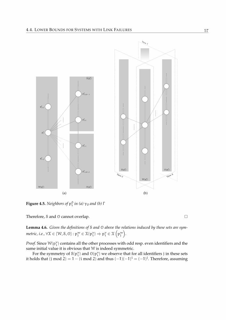
4.4. LOWER BOUNDS FOR SYSTEMS WITH LINK FAILURES
W(p0i ) O(p0
i )
S(p0i )
p0i−2
p0i
p0i+2
p0i−2`a+1
p0i−1
p0i+1
p0i+2`a−1
(a)
W(p0i )
S(p0i ) O(p0
i )
View XView 0
View 1
(b)
Figure 4.5. Neighbors of p0i in (a) γ0 and (b) Γ
Therefore, S and O cannot overlap.
Lemma 4.6. Given the definitions of S and O above the relations induced by these sets are sym-metric, i.e., ∀X ∈ W, S,O : pw
j ∈ X(pvi )⇒ pv
i ∈ X(pw
j
).
Proof. Since W(pvi ) contains all the other processes with odd resp. even identifiers and the
same initial value it is obvious that W is indeed symmetric.For the symmetry of S(pv
i ) and O(pvi ) we observe that for all identifiers j in these sets
it holds that (j mod 2) = 1 − (i mod 2) and thus (−1)(−1)i = (−1)j. Therefore, assuming

CHAPTER 4. DYNAMIC LINK FAILURES
that pvj ∈ S(pv
i ) we have
j = i+ (−1)i(1 + 2k + 2v`o) (mod n),
which leads to
−i =−j+ (−1)i(1 + 2k + 2v`o) (mod n),
multiplying by (−1) results in
i = j+(−1)(−1)i(1 + 2k + 2v`o) (mod n),
and finally we obtain
i = j+ (−1)j(1 + 2k + 2v`o) (mod n),
from which it follows that pvi ∈ S(pv
j ), since v all processes in S(pvi ) have the same initial
value tag v.The proof for the symmetry of O proceeds in the same way, by showing that j =
i − (−1)i(1 + 2k) (mod n) ⇔ i = j − (−1)j(1 + 2k) (mod n) and observing that whenpv
j ∈ O(pvi ), all members of O(pv
j ) have the initial value v = 1 − (1 − v) = v
The two lemmas above allow us to use the same techniques as above to prove theimpossibility of consensus, but without a fixed number of processes. Once again the ideais to assume an algorithm exists and to find subsystems that correspond to executionswhere the algorithm will violate Agreement when we assume that it achieves Validity.
Theorem 4.7. There is no deterministic algorithm that solves consensus in a system with n =
2`o + 4`a processes with up to `a arbitrary and `o omissive link faults per process per round andno process failures.
Proof. Suppose that there exists a distributed algorithm A that solves consensus under oursystem model with n = 2`o + 4`a. As before, we consider a system Γ with 2n processesand determine the “decision values” in this system by finding systems of n processes thathave communication graphs γ0, γ1, and γX, which are all covered by Γ . Thus the LocalityAxiom allows us to deduce that the decision values of processes in γ are the same as inthese n-process systems.
As a first step we determine the decision value of the processes p0i . To do so, we
consider the n process system in which all processes have the initial value 0 and whichuses the communication graph defined by γ0 (Figure 4.5(a)). Thus the links from p0
i to allprocesses in W(pv
i ) ∪ S(pvi ) are non-faulty, while those to processes in O(p0
i ) are arbitraryfaulty. (The links to the remaining processes are assumed to be purely omissive.) ByLemmas 4.5 and 4.6 this system abides to our failure assumptions, and due to the Validityof the assumed algorithm the decision value of all executions in this system must be0. One specific execution in γ0 is the one where the arbitrary faulty links carry exactlythe same messages as in Γ (Figure 4.5(b)), thus the processes p0
i all decide on 0 in Γ .Analogously, we can determine that the decision value of the processes p1
i in Γ must be 1.We now consider a third execution (referred to as Execution X) of n processes, where
half the processes have 0 and the other half has 1 as their initial value and the messagesreceived are exactly the same as in Executions 0 and 1. In the 2n system this executioncorresponds to the processes
p0
2k
∪p1
2k+1
with k < n
2 . These processes are collectively

4.5. UNIFYING LINK AND PROCESS FAULTS
p01 p0
0 p13 p1
2
p03 p0
2 p11 p1
0
p04 p0
5 p14 p1
5
p01
p03
View 0 View 1 View 0
View X
Figure 4.6. Drawing of an unrolled cube. (Nodes p03 and p0
1 are shown twice.)
referred to as the processes in View X. Recall that, in γX the links to processes in S arethose that are arbitrary faulty, while those to processes in O (and W) are considered non-faulty.
In the execution in the system defined by γX the decision value of processes in thesubsystem consisting of the processes
p0
2k
must be 0 due to the Locality Axiom and
the arguments about View 0 above. The processes inp1
2k+1
likewise still decide on
1. However, this behaviour violates Agreement in Execution X, thereby establishing therequired contradiction.
Note that this result also holds for the case where `a = 0, that is there are only ` = `o
omissive links per round per process. This is a somewhat paradoxical case, however, as∀p ∈ Π : S(p) = O(p) = ∅ when `a = 0. In other words, Γ and the γs are partitioned intocliques of size n
2 = `.
4.5. Unifying Link and Process faults
As the final lower bound of this section, we will show that in the presence of link faults (asdefined by our system model) it is impossible to reach consensus among n ≤ 2`o+4`a+2t
processes. On the one hand if t > 2`o + 4`a, the bound trivially follows from the n > 3t
lower bound given in Theorem 4.2. On the other hand, if link faults become too prevalentmore than 3t correct processes are be needed. We will show that this is necessary byextending Theorem 4.7 to show the aforementioned n ≤ 2`o + 4`a + 2t bound. Therefore,in general, there must be n > 2t+max t, 2` + 2`a processes to allow reaching consensus.Algorithm 5.1 and its proof of correctness will show that n > 2t + max t, 2` + 2`a isindeed sufficient.
Before considering the general case, we will first consider a simple extension of Theo-rem 4.3. More specifically, we examine the case where (at most) one process is faulty andevery process has one arbitrary faulty incoming/outgoing link. Thus, we have that t = 1
and ` = `a = 1, which leads to n = 6. To arrive at this number of processes, we extendthe cube of Theorem 4.3 by adding one process to each face. The definition of a view ischanged such that each view now comprises 6 (instead of 4) nodes. Figure 4.6 shows an“unrolled” cube with these extra processes, and how views are defined here.
Examining Figure 4.6 in more detail, we observe that in the executions corresponding

CHAPTER 4. DYNAMIC LINK FAILURES
to Views 0 and 1, the link between p0 and p3 as well as the link between p1 and p2 mustbe considered faulty. Nodes p4 and p5 have 5 correct links each, but the processor p5 isconsidered faulty.
As before, all processes in View 0 use v = 0 and therefore must decide 0 by the Validityproperty for the consensus algorithm running in the corresponding 6-process system.Similarly, in View 1, all processes must decide 1. Once again the processes in View X facea problem: Since for example process p0
0 observes exactly the same messages in View X
as in View 0, it must decide 0 as before. Similarly, as process p13 observes exactly the
same messages in View X as in View 1, it must decide 1. However, these decisions violateAgreement in the 6-process system corresponding to View X, thereby establishing therequired contradiction for completing the proof of Theorem 4.8.
Theorem 4.8. There is no deterministic algorithm that solves consensus with one arbitrary linkfault (` = `a = 1) and one Byzantine process (t = 1) fault in a system with n = 6 processes.
Turning to the general case, we first show that n > 2t + 2` + 2`a is needed to achieveconsensus, and then combine this result with the lower bound of Pease, Shostak, andLamport [Pease et al. 1980] to arrive at our final result, stated in Theorem 4.10 below.
Theorem 4.9. There is no deterministic algorithm that solves consensus for `a arbitrary linkfaults, `o purely omissive link faults and t arbitrary process faults in a system with n = 2t+2`+
2`a processes.
Proof. Suppose that there is an n processes execute a distributed algorithm A which solvesconsensus under our assumptions. In order to derive a contradiction, we once againarrange 2n processes in a graph, denoted Γ , as follows: First we build the graph ex-actly as described for the t = 0 case in Section 4.4, that is, for 2n ′ = 2(2` + 2`a) pro-cesses. Then we add for each v two sets of processes E[v] = pv
i | n ′ ≤ i < n ′ + t andF[v] = pv
i | n ′ + t ≤ i < n ′ + 2t. (These sets play the roles of pv4 and pv
5 in the argu-ment for Theorem 4.8.) Processes in E[v] are connected to all processes in View v, thatis, all pv
i with 0 ≤ i < n. Processes in F[v] are connected to all processes in Viewv except those in pv
i | i mod 2 = 1 ∧ i < n ′. Instead, we connect processes in F[v] top1−v
i | i mod 2 = 1 ∧ i < n ′. Thus, each process in F[v] has connections to processes inthe set pw
i | (0 ≤ i < n ′) ∧ (w = v + i mod 2)∪E[v]∪F[v]. In summary, we add two sets(to each view) of processes instead of only two processes as in Figure 4.6 and connectthem analogously. We observe that when adding the 2t processes, we do not add anymore faulty links to the executions corresponding to any of the views and therefore Lem-mas 4.5 and 4.6 still apply here. Note that in the executions corresponding to the views 0
and 1 all processes in the E sets are correct, while those in the F sets behave faulty. Thisconcludes the construction of our 2n process system, with views 0 and 1, each of whichcorresponds to an execution of n = 2t + 2` + 2`a processes.
Now — once again — for v ∈ 0, 1, consider the processes in Views v, which all haveinitial value v, respectively. By applying the Validity property of A to the executions inγv all processes must decide on v. To reach the desired contradiction, we now have tochoose n processes in Γ , such that their perceptions and behaviour correspond to a validExecution X in the n process system whose communication graph is γX. This can be

4.5. UNIFYING LINK AND PROCESS FAULTS
achieved by selecting the processes in
X = E[0] ∪ F[0] ∪
p0i | (i mod 2 = 0) ∧ (i < n ′)
∪
p1i | (i mod 2 = 1) ∧ (i < n ′)
.
Since there are processes with different initial values in X and all processes have todecide on their initial value by the construction above, we have reached the contradictionif we can show that X can be mapped to a valid γX. This is done in two steps: We firstshow that (i) X is indeed a set of n distinct processes, and (ii) that our failure assumptionsare not violated in X.
As for (i) we observe that the sets that make up X are all non-overlapping with respectto their identifiers. The sets E[0] and F[0] are of size t each, while the last two componentsare of size n ′
2 each. This adds up to n ′ + 2t = n processes. As for (ii) we observe thatin View X (in contrast to the Views v) processes in F[0] are perceived in the same way byall processes. That is, they can be counted as correct processes with correct links only. InExecution X the t processes in E[0] have to be considered Byzantine, since the asymmetricbehaviour3 of those processes exceeds what could be attributed to link failures. As wecan blame all asymmetric behaviour on the processes being faulty, the outgoing links ofE[0] do not count towards the `a limit on the incoming links of neighbors. As for theincoming links of E[0], we note that we can do not have to check the link failure boundsas these apply only to correct processes. For the other two subsets of X we observe thatall processes are correct, and that these processes alone correspond to a valid View X in a2n ′ system (as in Lemma 4.5). Therefore (ii) holds as well.
What remains, is to relate the result of Theorem 4.9 with the result of Theorem 4.2.Obviously, the resilience-bounds which can be deduced from the two theorem must bothbe guaranteed in order to have a system in which consensus is solvable. Or the otherway round, when one of them is not fulfilled consensus remains unsolvable. Thus weconclude this chapter with the observation that,
Theorem 4.10. There is no deterministic algorithm that solves consensus with `a arbitrary linkfaults, `o purely omissive link faults and t arbitrary process faults in a system with n ≤ 2t +
max t, 2` + 2`a processes.
At this point the question of how the results of this chapter relate to other impossibil-ity results for link failures naturally arises. One point that is interesting is that while wehave assumed that the faulty links may change from round to round, this fact is not usedin the proofs. This is in contrast to Santoro and Widmayer [1989], who assume that thetransmission failures may occur in a block around different processes in different rounds.(Informally their impossibility result is thus based on a similar construction as that of Fis-cher et al. [1985], where the process unable to communicate “in time” to others changesover time as well.) Moreover, Santoro and Widmayer require only n−1 omissions or
⌈n2
⌉Byzantine faulty links system-wide in each round, whereas ` > n
2 omissions or ` > n4
Byzantine faulty links are required per process for our construction to work. Therefore,none of the two results is more general.
3This asymmetric behaviour is caused by some processes receiving the same messages from E[0] in Exe-cution X as they received from E[0] in Γ , while others receive the same messages as they received from E[1]
in Γ .


P A R T
IIIA L G O R I T H M S


C H A P T E R 5
R E T R A N S M I S S I O NP R O T O C O L S
IN THE PREVIOUS Chapter we proved a lower bound on the number of processes re-
quired to solve consensus in the presence of Byzantine processes and a certain classof moving link failures (cf. Theorem 4.10). This naturally leads to the question whetherthe given bound is tight. Instead of finding a matching consensus algorithm, we willshow how to mask these link failures in an optimal way. By combining an (optimal) reli-able channel simulation with an optimal consensus algorithm, that requires reliable links,we obtain an optimal solution for consensus with respect to resilience. When we talkabout channels in the following, we mean simulated entities connecting processes overthe (physical) links. Similar to reliable links (cf. Chapter 2), a channel is reliable when ev-ery message that is sent over the channel by a non-faulty process is received exactly once(at any non-faulty receiver). This definition assumes uniquely identifiable messages, aswhen two messages with the same content are sent, each of the two (identical) messagesis required to be delivered once. Moreover, messages from correct processes are deliveredonly if the message was really sent by that correct process.
Our implementation of reliable channels will use two rounds of communication thusdoubling the termination time of any algorithm (and increasing the message load n-fold).It is similar to the simulated authentication algorithms of Srikanth and Toueg [1987a],which has been used to solve a wide range of agreement problems [Srikanth and Toueg1987a; Toueg et al. 1987; Srikanth and Toueg 1987b; Dwork et al. 1988]. In Section 5.2, weshow how the properties of both reliable channels and simulated authenticated messagescan be achieved in three rounds per broadcast (instead of four as one would need whensimply plugging the two simulations together. Note that these are simulations in thesense of Chapter 12 in the book by Attiya and Welch [2004] and the work by Neiger andToueg [1990] and not algorithm transformations (recall Chapter 3), with the most promi-nent difference being that with simulations one can use multiple independent threads ofcontrol as one is not bound to providing replacements for operations.
We use the same model as in the previous chapter for our analysis. Using this veryrestrictive model has the advantage that we can focus on how failures are masked in thealgorithms and proofs. That is, we assume a system with a communication-closed round

CHAPTER 5. RETRANSMISSION PROTOCOLS
structure, up to t faulty processes and up to ` incoming/outgoing faulty links per roundand per process (of which `a may be value faulty). Note, however, that the round modelswe implement are communication-open when there are Byzantine failures. Without suchfailures there the resulting round structure would be communication-closed as well. Thisis due to the fact that only faulty processes can cause enough asymmetry for processes todeliver a message in different rounds.
5.1. Masking Link Failures
In general a channel from a sending process to a set of receivers is reliable, if it guaranteesthe following properties with respect to some message msg:
Channel Validity: If a correct process sends msg, then all correct receivers eventuallydeliver msg.
Channel Integrity: Every correct receiver delivers msg at most once, and only if someprocess actually sent msg.
Our definition of a reliable channel is equivalent to the Validity and Integrity proper-ties of a reliable broadcast as defined by Hadzilacos and Toueg in their chapter on broad-casting in Mullender’s book [1993]. Besides the two properties above they also introducea property called Agreement, which — in short — requires relaying (cp. the propertiesdiscussed in Section 5.2). Omitting this property has no impact as long as senders and re-ceivers are correct. Link faults that occur on links where either the sender or the receiveris faulty may still exhibit arbitrary behavior/message loss, but these effects can safely beattributed to the faulty process.1 Consequently, our channel does not guarantee that allreceivers agree on the delivered value if the sender was faulty, thus contrasting reliablebroadcast [Hadzilacos and Toueg 1993].
As mentioned before, the definition of Channel Integrity implies that all messagesare unique. Often it is reasonable to assume that all messages are unique, as it can beenforced by using unique sequence numbers for every message. Since the link failures wewould like to tolerate are defined for round-based systems only, we do not keep sequencenumbers explicitly, but rather use round numbers.
As our reliable channel implementation (and the authenticated channels presented inSection 5.2) are based on rounds, and the algorithms using them are so as well, we needto find a concept that allows us to discriminate between the two. Thus, we will in thischapter refer to micro- and macro-rounds. The micro-rounds are what our channel im-plementations use, while the algorithms built atop these channels will use macro-rounds.A macro-round ends after k micro-rounds. (For our reliable channel implementationk = 2.) That is, the code of the macro-round ρ is executed when the (micro-) roundcounter reaches kρ.
For simplicity, we assume that the algorithm using our channel implementation isbroadcast based. In the above reliable channel properties there is no notion of rounds, aswe are concerned about round-based systems, we prove the following variant of Chan-nel Validity, which is stronger in such systems (but, as it refer to rounds, not as general).
1This is due to the fact that links from benign faulty processes can only loose messages, while arbitrarylink failures are only possible with Byzantine processes.

5.1. MASKING LINK FAILURES
1: variables2: r ∈ N // the current macro-round3: ∀q ∈ Π, delivered[q]← ∅ // the set of rounds for which we have delivered messages from q
4: procedure reliably-send(msg)
5: send(INIT, p, msg, r) to all nodes [including itself]
6: thread reliably-receive :
7: in each micro-round:8: if received(INIT, q, msg, k) from q in micro-round 2k then9: send(ECHO, q, msg, k) to all nodes [including itself]10: if received(ECHO, q, msg, k) from n − t − 2` distinct processes in one micro-round then11: if k 6∈ delivered[q] then12: delivered[q] = delivered[q] ∪ k
13: reliably-deliver(msg, q, k)
Algorithm 5.1. Reliable Channel Implementation, code for process p
Moreover, as a process may send the same message in multiple rounds, we prove a vari-ant of Channel Integrity which captures this fact.
Channel Validity’: If a correct process sends msg in macro-round r, then all processesdeliver msg in macro-round r.
Channel Integrity’: Every correct receiver delivers msg only for those rounds in which itwas sent msg.
Our reliable channel implementation (Algorithm 5.1) proceeds as follows: To reliablysend a message on the channel to a receiver, the sending process uses the reliably-sendfunction (line 4 ff.). The reliably-receive thread runs at all processes and forwards themessage to the designated receiver(s), where the thread will also deliver it to the nextprotocol level through reliably-deliver.
One particularly important detail of Algorithm 5.1 (and Algorithm 5.2) is that it re-sends all messages in every round and only uses messages received in the current roundin its rules. This is necessary, because link failures can produce `a erroneous ECHO-messages per round at any correct process, which could otherwise accumulate over mul-tiple rounds to surpass any threshold.
Theorem 5.1. Algorithm 5.1 guarantees a reliable channel between each correct sender and allcorrect receivers, if n > 2t + 2` + 2`a.
Proof. We denote the sending process by s. We show each of the two properties separately,splitting the proof into two parts:Channel Integrity’: A correct process only delivers a messages if it has received at leastn − t − 2` copies of a ECHO-message from distinct processes. We observe that sincen > 2t + 2` + 2`a this corresponds to at least t + 2`a + 1 echo messages corresponding tothe message to be delivered.
Recall that (i) at most t processes are arbitrary faulty, (ii) at most `a (correct) processescan receive an INIT-message from s out of thin air (that is, without s sending such mes-sage) and thus respond with corresponding ECHO-messages, and (iii) each receiver canreceive at most `a ECHO-messages from processes, which never sent them. This resultsin at most t + 2`a < n − t − 2` ECHO-messages which can be received by some receiver

CHAPTER 5. RETRANSMISSION PROTOCOLS
if s has not sent an INIT-message. Therefore it is clear that a process will only deliver amessage if the sender has sent the INIT-message. As the original macro-round number isattached to all INIT- and ECHO-messages, a message clearly is only delivered for a round,for which it was sent. Moreover, adding the round number to the set delivered[s], when amessage from s is delivered, ensures that the message is delivered only once.Channel Validity: Since — by assumption — s is correct, it sends the same message to allprocesses p ∈ Π. There are at least n − t − ` correct processes that receive the messages has sent and will therefore forward corresponding ECHO-messages to the all processes(line 9). Thus, each correct process will receive at least (n − t − `) − ` = n − t − 2` andwill therefore, execute the code following line 10. This takes exactly two micro-roundsand thus one macro-round.
From this theorem it follows that by using our reliable channel implementation (Al-gorithm 5.1) for communication and any consensus algorithm that requires n > 3t (ex-amples include the work by Pease et al. [1980], Dwork et al. [1988], Garay and Moses[1993], and Dolev et al. [1982]) one can solve consensus in the presence of link faults inaccordance to our assumptions with n > 2t + max t, 2` + 2`a. These possibility resultsindicate that the lower bound of Theorem 4.10 is tight; respectively the impossibility ofTheorem 4.10 indicates that these consensus solutions are optimal with respect to theirresilience.
5.2. Authenticated Channels
In this section we turn our attention from simulating reliable channels to simulating au-thentication. One way to implement authenticated channels is by means of signed mes-sages (e.g., [Rivest et al. 1978; NIST 1992]). This leads to problems, however, when oneconsiders Byzantine faults. In general Byzantine faults are assumed to be able to sendmessages with any content. In the context of cryptography based authentication thisis no longer true, as in order to make signatures useful Byzantine processes must be as-sumed to be unable to (erroneously) send messages containing data with valid signaturesof other processes (unless the other process has signed that data before). Such an assump-tion clearly precludes finding a simple formal definition of Byzantine behaviour in mod-els with authentication [Lynch 1996, page 115]. Moreover, cryptography involves com-putationally expensive operations, which cannot always be afforded in power-limitedsystems.
This makes the non-authenticated implementation of the broadcast primitive devel-oped by Srikanth and Toueg [1987a] attractive. Instead of using cryptography, their sim-ulated broadcast primitive relies upon the idea of letting all processes witness a process’smessage broadcast. As mentioned above, one could combine the reliable channel im-plementation of Section 5.1 with their primitive, leading to each broadcast taking fourrounds. Instead we present an alternative primitive which achieves the properties ofauthenticated channels in three rounds.
The definition of the authenticated reliable broadcast of message m by process s inround k is based on (i) the broadcast primitive authenticated-broadcast(m) and (ii) the re-ception callback authenticated-accept(s,m, k). The semantics of the broadcast primitive arefully captured by the following three uniform properties [Hadzilacos and Toueg 1993]:
Correctness: If a non-faulty process p executes authenticated-broadcast(m) in round k,

5.2. AUTHENTICATED CHANNELS
1: variables2: r ∈ N // the current macro round number3: witness(s, m, k) // the set of processes who witnessed s sending m in round k
4: procedure authenticated-broadcast(m)
5: send(INIT, r, m) to all nodes [including itself]
6: thread authenticated-receive :
7: in each micro-round:8: if received(INIT, k, m) from s in round k then9: send(ECHO, k, s, p) to all nodes [including itself]10: if received(ECHO, k, m, s, q) from q in some round ≥ k then11: send(confirm, k, m, s, q) to all nodes [including itself]12: if received(confirm, k, m, s, q) from at least n − t − 2` distinct processes in some round ≥ k then13: witness(s, m, k) = witness(k, m, s) ∪ q
14: if |witness(s, m, k)| ≥ n − t − ` then15: authenticated-accept(s, m, k)
Algorithm 5.2. Broadcasting primitive for simulated authentication, code for process p
then every correct process executes authenticated-accept(p,m, k) in the same round.
Uniform Unforgeability: If a correct process p never executes authenticated-broadcast(m),then no correct process ever executes authenticated-accept(p,m, k).
Uniform Relay If a correct process executes authenticated-accept(p,m, k) in round r ≥ k,then every correct process also executes authenticated-accept(p,m, k) in round r + 1
or earlier.
Note that the late delivery of the relay property can (by definition) only occur, if theinitial broadcaster p is faulty. In fact, the collusion of a faulty broadcaster with faultywitnesses could defer the delivery of a message (through authenticated-accept) arbitrarilylong;, it could even prohibit termination of the broadcast (this was also noted by Srikanthand Toueg [1987a] for their broadcasting primitive). However, this can only happen if nocorrect process has accepted the message in question yet, as otherwise, the relay prop-erty would ensure that all correct processes accept the message by the end of the roundfollowing acceptance by the first non-faulty process.
One particularly important detail of Algorithm 5.2 is that it re-sends all messages inevery round and only uses messages received in the current round in its rules. This isnecessary, because link failures can produce `a erroneous (echo, p,m, k) messages perround at any correct process, which could otherwise accumulate over multiple rounds tosurpass any threshold.
In our first lemma, we prove what can be seen as variants of the Correctness andUnforgeability properties, which are concerned with the some process p sending of anECHO message and p being added to the set witness at all correct processes.
Lemma 5.2. When (i) a correct process p sends an ECHO message (for some broadcast) everycorrect process adds p to its set of witnesses at most two micro-rounds later. When (ii) a correctprocess p never sends an ECHO message for some broadcast then no correct process ever adds p
to its witness set for that broadcast, provided that n > 2t + 2` + 2`a.
Proof. (i) When the correct process p sends an ECHO for a message, all but ` correct pro-cesses will receive it and respond with a confirm message. Every correct process thus

CHAPTER 5. RETRANSMISSION PROTOCOLS
receives n − t − 2` confirmations for p’s ECHO message, and thus add p to their witnessset for the message.(ii) When process p does not send an ECHO for some broadcast, at most t + `a will “re-spond” with sending a confirm message, which allows for t + 2`a such messages to bereceived at any correct process. This, however, does not suffice to cause any correct pro-cess to add p to its witness set, or perform any other action, that might cause this indirectly(because t + 2`a < n − t − 2`).
Theorem 5.3 (Simulated Broadcast). Correctness, Unforgeability and Relay hold with 3 micro-rounds per macro-round assuming n > 2t + ` + `a + max(t, ` + `a).
Proof. Correctness: When a correct process s sends INIT, then all correct processes except` receive that message. All those processes respond with an ECHO message tagged withtheir own identifier. By Lemma 5.2 they get all added to the witness set at each correctprocess. These sets thus have at least n − t − ` members which causes the message sentby s to be delivered within 3 micro-rounds, or one macro-round.Unforgeability: If s does not send an INIT message for some message m in round r, thenno correct process (except `a) will send a matching ECHO message. That is, at most t+ `a
processes send ECHO messages. From (ii) in Lemma 5.2 it follows that at most `a correctprocesses will be added to the witness set for this message. Therefore, the maximum sizeof such a set is bounded by t + `a, which in turn implies that the message cannot bedelivered, since t + `a < n − t − `.Relay: When some (correct) process delivers s,m, k then at least n − t − ` processes mustbe in its witness set for this message. From (ii) in Lemma 5.2, it follows that all correctprocesses (at least n − t − ` − t) in the witness set must have sent an ECHO message.Therefore, by (i) in Lemma 5.2 every correct process has at least n − t − ` − t > t + `a
processes in its witness set. This implies that every correct process will send an ECHO
message. When all correct processes send ECHO messages, every correct process willadd every correct process into its witness set, and thus this set will surely grow to n − t >
n − t − ` processes, resulting in the delivery of the message at most two micro-roundslater. Since these two micro-rounds may span over a macro-round change, the deliverymay occur only in the next macro-round.
By combining n − t − ` − t > t + `a, (i.e., n > 3t + ` + `a) as required for Relay (andUnforgeability) and n > 2t + 2` + 2`a as required for Lemma 5.2, one obtains a bound ofn > 2t + ` + `a + max(t, ` + `a).
By plugging in the hybrid simulated broadcast primitive of Algorithm 5.2 into anByzantine agreement algorithm assuming authentication one gets a non-authenticatedalgorithm for Byzantine agreement that tolerates Byzantine process and both arbitraryfaulty and lossy links. In particular, one could choose the algorithm used by Srikanthand Toueg [1987a] (or for that matter the original one by [Dolev and Strong 1982b]).Since these algorithms require n > t only, the composed protocol “inherits” the resiliencebound n > 2t + ` + `a + max(t, ` + `a) from our broadcasting primitive. Moreover, thetwo algorithms can even be simplified: the algorithms explicitly forward all messagesthey receive after adding their signature. This is in fact not necessary, due to the relayproperty, which performs this forwarding implicitly.
C H A P T E R 6
AT,E A N D H E RI M P L E M E N TAT I O N
Although originally considered only for synchronous systems round models can provideuseful abstractions for capturing the synchrony in general systems. (This is exemplifiedby the results of Chapter 3.) In the context of not fully synchronous systems one can sep-arate round models into two classes depending on what happens with messages that didnot arrive within a round. As already mentioned the model presented in Section 3.2.4 isan example of a communication open model as late messages are simply delivered when-ever they arrive in later rounds. Informally one could say that the processes are alwaysopen to receive late information. The alternative are communication closed models [Elradand Francez 1982] in which messages are never delivered after the round they were sentin has ended. That is, late messages are simply discarded. This approach has the advan-tage that not only synchrony but also reliability of communication can be captured in thesame way, as there is no difference between a late, a lost, and a message never sent. Thisis the idea behind the Heard-Of Model [Charron-Bost and Schiper 2006a; Charron-Bostand Schiper 2009], which provides a framework for modelling different system assump-tions based on predicates on HO(p, r) sets, that is, the set of processes p has heard of inround r model. As the reasons for some process q not being in HO(p, r) are completelyabstracted away, q cannot be the culprit. In other words, there are no faulty processes inthe HO-model.
We show that this approach can be generalized for systems with non-benign failures[Biely et al. 2007a]. Typically a process cannot distinguish whether a faulty messageoriginates from a communication fault and from to a process fault. Therefore, from analgorithm designer’s point of view the important information is how many of the mes-sages received in a round can be trusted. This can be captured by the safe heard-of setSHO(p, r) which comprises those processes p has correctly received information from inround r. Clearly, unlike the HO set this set is not known to the process at run-time. Thealgorithm can only rely on the assumptions made about the size of this set.
So while the heard-of sets capture liveness of communication, one can regard thesafe heard-of sets to capture communication safety. These collections of sets allow usto specify sufficient conditions for solving consensus in such a system. We will deter-
CHAPTER 6. AT,E AND HER IMPLEMENTATION
mine predicates sufficient for solving consensus with a certain algorithm in Section 6.2.We will then look into a lower level model (based on a generalization of the partiallysynchronous model [Dwork et al. 1988]) and try to implement these predicates. Unfortu-nately, due to formal reasons and the particularities of the model we will have to give upthe clear separation between the round model implementation and the consensus algo-rithm. Informally, the problem is that it is not possible to guarantee that a process is not“in the same round twice” in our model.
6.1. Heard-Of Sets and Communication Predicates
Computations in our model are structured in rounds, which are communication-closedlayers. Algorithms in the round model consist of the following components (for eachprocess p): the set of possible states denoted by statesp, a subset initp of initial states, andfor each positive integer r called round number, a message-sending function Sr
p mappingstatesp×Π to a unique message from M, and a state-transition function T r
p mapping statesp
and partial vectors (indexed by Π) of elements of M to statesp. The collection of algorithmsfor the processes is called an algorithm on Π.
Each process p progresses through the computation by iterating through rounds r ∈N. In each round r, a process p will
1. apply Srp to the current state sr
p, and emit the “messages” to be sent (according toits sending function Sr
p) to each process;2. then determine the partial vector ~µ r
p, formed by the messages that p receives inround r;
3. apply T rp to its current state and ~µ r
p, which yields sr+1p .
Mapping this behaviour to the generic model of Chapter 2 is pretty straightforward:We only have to define how the above course of action is mapped to steps. The simplestassumption is to assume that processes perform all three items in one step. However, asmessages are in transit between the first two items, we assume that one step consists ofreceiving the messages of round r, then applying T r
p, and finally sending the messagesdetermined by Sr+1
p . Recall that in the HO-model there is not notion of faulty processes,which nicely matches our assumption in the generic model that processes always followtheir algorithm. As HO-algorithms are based solely on the sets of received messages(or rather guarantees about them), we abstain from giving the reasons for missing orcorrupted messages. In other words, we do not provide detailed failure assumptions atthis level of abstraction. (We will do so in Section 6.3, however.)
The partial vector ~µ rp is called the reception vector of p at round r. The state sr
p a processis in at the beginning of round r is subsequently also referred to as p’s round r state. Forany part of this state, that is any variable xp local to process p, we denote x
(r)p the value
of xp in srp, i.e., at the beginning of round r.
Each run is entirely determined by the initial configuration (i.e., the collection of pro-cess initial states), and the collection of the reception vectors
(~µ r
p
)p∈Π, r>0
. For each pro-cess p and each round r, we introduce two subsets of Π:
• The heard-of set, denoted HO(p, r), which is the support of ~µ rp, i.e.,
HO(p, r) =q ∈ Π : ~µ r
p[q] is defined
.

6.1. HEARD-OF SETS AND COMMUNICATION PREDICATES
• The safe heard-of set, denoted SHO(p, r), and defined by
SHO(p, r) =q ∈ Π : ~µ r
p[q] = Srq(sq, p)
.
Both sets specify the difference between what should be sent and what is actually re-ceived. As for the benign case [Charron-Bost and Schiper 2009], we make no assumptionon the reason why ~µ r
p[q] 6= Srq(p, sq): it may be due to an incorrect sending by q, an
incorrect receipt by p, or due to the corruption by the link from q to p. Obviously, wehave SHO(p, r) ⊆ HO(p, r). In contrast to HO(p, r), process p is not able to determineSHO(p, r).
From the two sets HO(p, r) and SHO(p, r), we form the altered heard-of set denotedAHO(p, r) as follows:
AHO(p, r) = HO(p, r) \ SHO(p, r).
For any round r we can define the altered span denoting the set of processes fromwhich at least one process received a corrupted message, and we can then extend thisdefinition to whole executions:
AS(r) =⋃p∈Π
AHO(p, r) AS =⋃r>0
AS(r)
6.1.1. HO Machines
A heard-of machine for a set of processes Π is a pair 〈A,P〉, where A is an algorithmon Π, and P is a communication predicate, i.e., a predicate over (HO(p, r))p∈Π, r>0 and(SHO(p, r))p∈Π, r>0 .
As an example, we can model the classical assumption, that no more than α processesmay send a corrupted information in a computation:1
Ppermα := |AS| ≤ α (6.1)
For our algorithms we will consider the weaker predicate Pα that restricts the numberof corrupted messages only per round and per process:
Pα := ∀r > 0,∀p ∈ Π : |AHO(p, r)| ≤ α (6.2)
with α ∈ R such that 0 ≤ α ≤ n, and we say that a computation has α-safe communicationswhen Pα holds. Note that P
permα implies Pα.
We will consider only communication predicates, that are time-invariant: A commu-nication predicate P is time-invariant if it has the same truth value for all heard-of col-lections (HO(p, r + i))p∈Π,r>0 and (SHO(p, r + i))p∈Π,r>0 for any i ∈ N. This allowsprocesses to start in their execution in any round r, while preserving the truth value of P.The predicates P
permα and Pα are trivially time-invariant, since they are permanent pred-
icates. Time-invariant predicates that characterize eventual properties typically have theform
∀r > 0 ∃r0 > r : Pr0,
1Note that in the classical “Byzantine” setting, also the state of a “faulty” process can be corrupted, whichis not the case in our model. Refer to Chapter 7 for a discussion.

CHAPTER 6. AT,E AND HER IMPLEMENTATION
where Pr0is a predicate over the collection (HO(p, r); SHO(p, r))p∈Π. In other words,
such properties always hold eventually, which contrasts the time-variant predicate ∃r0 >
0 : Pr0which may only holds once.
HO-machines for the benign case [Charron-Bost and Schiper 2009] can be seen as aspecial case of the above definition, with AS = ∅, which is equivalent to assuming thepredicate
Pbenign := ∀p ∈ Π,∀r > 0 : SHO(p, r) = HO(p, r).
6.1.2. Consensus
Since, contrary to classical approaches, there is no deviation according to T rp, that is, there
is no notion of a faulty process, we have to adapt the formulation of the consensus prob-lem such that it holds for all processes. Thus we get the following properties:
Validity: If all processes have the same initial value this is the only possible deci-sion value.
Agreement: No two processes may decide differently.Termination: All processes eventually decide.
Formally, an HO machine 〈A,P〉 solves consensus, if any run for which P holds, satis-fies Validity, Agreement, and Termination. To make this definition non-trivial, we assumethat the set of HO and SHO collections for which P holds is non-empty.
6.2. The AT,E algorithm
In this section we present the AT,E algorithm, and determine the predicates under whichit is correct. The code of AT,E is given as Algorithm 6.1.
In AT,E each process p maintains a variable xp initially equal to p’s initial value. Ateach round, process p broadcasts xp, and if it receives more than T (“Threshold”) mes-sages, updates xp, by setting xp to the smallest of the values it has received the mostfrequently. If p has received more than E (“Enough”) times the same value v, then itdecides on v.
Basically, it consists in a parametrization of the two “receive thresholds” T and E ofthe OneThirdRule algorithm [Charron-Bost and Schiper 2006a; Charron-Bost and Schiper2009] for solving consensus in the presence of benign failures (there both are equal to2n3 ). The main features of OneThirdRule are: (i) the algorithm is always safe2, whatever
the number of benign transmission faults is, and (ii) the algorithm is fast in the sense thatit requires two rounds to terminate in every failure-free run, and further it terminates atthe end of the first round if all initial values are equal. In the sequel, we show that, forappropriate choices of T and E, the AT,E algorithm both tolerates a large number of benignfaults (omission) and non-benign faults (corruption), while retaining the main features ofOneThirdRule. Contrary to OneThirdRule AT,E is not always safe, but requires a predicatelimiting the amount of corrupted communication a process can receive (the predicate iscalled Pα and is introduced above in Equation (6.2)). For deciding AT,E requires a secondpredicate to hold as well, which is of the eventual flavour and referred to as PA,live andgiven in Figure 6.1.
2By the algorithm being always safe, we mean that the safety properties of consensus (namely, Validityand Agreement) are guaranteed even in asynchronous runs.

6.2. THE AT,E ALGORITHM
1: Variable Initialization:2: xp ∈ V , initially vp // vp is the initial value of p
3: Round r :4: Sr
p:5: send 〈 xp 〉 to all processes6: Tr
p:7: if |HO(p, r)| ≥ T then8: xp := the smallest most frequently received value9: if at least E values received are equal to v then10: DECIDE(v)
Algorithm 6.1. The AT,E algorithm
∀r0 > 0, ∃r ≥ r0, ∃Π1r , Π2
r ⊆ Π s.t.(˛Π1
r
˛≥ E − α) ∧ (
˛Π2
r
˛≥ T) ∧ (∀p ∈ Π1
r , HO(p, r) = SHO(p, r) = Π2r)
∧
∀r > 0, ∀p ∈ Π, ∃rp > r : |HO(p, rp)| ≥ T
∧
∀r > 0, ∀p ∈ Π, ∃rp > r : |SHO(p, rp)| ≥ E
Figure 6.1. Predicate PA,live
6.2.1. Correctness of the AT,E algorithm
First we introduce some notation. For any value v ∈ V and any process p, at any roundr > 0, we define the sets Rr
p(v) and Qrp(v) as follows:
Rrp(v) :=
q ∈ Π : ~µ r
p[q] = v
Qrp(v) :=
q ∈ Π : Sr
q(p, srq) = v
.
In words, the set Rrp(v) represents the set of processes from which p receives v in
round r, while Qrp(v) is the set of processes that ought to send v to p in round r. Since
every process sends the same message to all in AT,E, the sets Qrp(v) do not depend on p,
and so can be just denoted by Qr(v) without any ambiguity.We start our correctness proof with a general basic lemma.
Lemma 6.1. For any process p and any value v, at any round r, we have:∣∣Rrp(v)
∣∣ ≤ |Qr(v)| + |AHO(p, r)| .
Proof. Suppose that process p receives a message with value v at round r > 0 from processq. Then, either the code of q prescribes it to send v to p at round r, i.e., q belongs to Qr(v)
and thus q is also in SHO(p, r), or the message has been corrupted and q is in AHO(p, r).It follows that
Rrp(v) ⊆ Qr(v) ∪ AHO(p, r),
which implies ∣∣Rrp(v)
∣∣ ≤ |Qr(v)| + |AHO(p, r)| .
Lemma 6.1 naturally leads to consider the communication predicate Pα from (6.2): Pα
bounds the size of AHO(p, r), that is limits the discrepancy between the sets Rrp and Qr.
Our second lemma shows that choosing E ≥ n2 renders the decision rule in the AT,E
algorithm “deterministic”.

CHAPTER 6. AT,E AND HER IMPLEMENTATION
Lemma 6.2. If E > n2 , then the guard in line 9 of the AT,E algorithm is true for at most one value
v.
Proof. Assume by contradiction that there exist a process p and a round r, so that theguard in line 9 is true for two distinct values v and v ′. The code implies that
∣∣Rrp(v)
∣∣ ≥ E
and∣∣Rr
p(v ′)∣∣ ≥ E. Since v and v ′ are different, Rr
p(v) and Rrp(v ′) are disjoint sets, and so∣∣Rr
p(v) ∪ Rrp(v ′)
∣∣ =∣∣Rr
p(v)∣∣ +
∣∣Rrp(v ′)
∣∣ .
From E > n2 we have
∣∣Rr0p (v) ∪ R
r0p (v ′)
∣∣ > n, a contradiction.
As an intermediate step to argue agreement, our next lemma shows that a strongercondition on E ensures no two processes can decide differently at the same round:
Lemma 6.3. If E > n2 + α then in any run of the HO machine 〈AT,E,Pα〉 there is at most one
possible decision value per round.
Proof. Assume by contradiction that there exist two processes p and q that decide ondifferent values v and v ′ in some round r > 0. From the code of AT,E, we deduce that∣∣Rr
p(v)∣∣ ≥ E and
∣∣Rrq(v ′)
∣∣ ≥ E. Then Lemma 6.1 ensures that |Qr(v)| ≥ E−α and |Qr(v ′)| ≥E − α when Pα holds.
Since each process sends the same value to all at each round r, the sets Qr(v) andQr(v ′) are disjoint if v and v ′ are distinct values . Hence |Qr(v) ∪Qr(v ′)| = |Qr(v)| +
|Qr(v ′)|. Consequently, when E > n2 +α, we derive that |Qr(v) ∪Qr(v ′)| > n, a contradic-
tion.
The next lemma ensures that for sufficient large T , once a process has decided, otherprocesses may learn only the decision value in that round:
Lemma 6.4. If T > 2(n + 2α − E), then in any run of the HO machine 〈AT,E,Pα〉 such thatprocess p decides value v at round r0, every process q that updates its variable xq at round r0 setsit to v.
Proof. Suppose that process p decides value v at round r0 > 0. Let q be any process suchthat |HO(q, r0)| ≥ T , i.e., q modifies xq at round r0. Let Qr0(v) denote the set of processesthat, according to their sending functions, ought to send messages different from v atround r0, and let R
r0q (v) denote the set of processes from which q receives values different
from v at round r0. Since each process sends a message to all at each round, Qr0(v) =
Π\Qr0(v), and thus |Qr0(v)| = n− |Qr0(v)|. Similarly, we have Rr0q (v) = HO(q, r0)\R
r0q (v),
and since Rr0q (v) ⊆ HO(q, r0), it follows that
∣∣Rr0q (v)
∣∣ ≤ T − Rr0q (v).
Since p makes a decision at round r0, by line 7,∣∣Rr0
p (v)∣∣ > E. Then Lemma 6.1 implies
|Qr0(v)| > E − α, from which |Qr0(v)| < n − (E − α) follows. With an argument similar tothe one used in the proof of Lemma 6.1, we derive that
∣∣Rr0q (v)
∣∣ ≤ |Qr0(v)| + |AHO(q, r0)|.When Pα holds, we obtain
∣∣Rr0q (v)
∣∣ ≤ n + 2α − E.From
∣∣Rr0q (v)
∣∣ ≤ T − Rr0q (v) it follows that in order to ensure
∣∣Rr0q (v)
∣∣ >∣∣Rr0
q (v)∣∣ then
one needs T > 2(n + 2α − E). This implies that v is the most frequent value received by q
at round r0. Then the code entails q to set xq to v.
We now extend the statement of Lemma 6.4 to hold also for any round after the deci-sion:

6.2. THE AT,E ALGORITHM
Lemma 6.5. If T > 2(n + 2α − E), then in any run of the HO machine 〈AT,E,Pα〉 such thatprocess p decides some value v at some round r0 > 0, every process q that updates its variable xq
at some round r ≥ r0 necessarily sets it to v.
Proof. Assume process p decides value v at round r0 > 0. Let q be some process thatupdates xq at some round r ≥ r0. Assume for now that
|Qr(v)| =∣∣∣p ′ : x
(r−1)p ′ = v
∣∣∣ ≥ E − α, (6.3)
then the same argument as in Lemma 6.4 applies, and so the code entails q to set xq to v
at round r. In order to show (6.3) we use induction on r:
Base case: r = r0. Since p decides v at round r0, we have∣∣Rr0
p (v)∣∣ ≥ E. By Lemma 6.1, we
get |Qr0(v)| ≥ E − α when Pα holds. Moreover we know (from the code of AT,E)that Qr0(v) =
p ′ ∈ Π : x
(r0)p ′ = v
, and so the base case follows.
Inductive step: r > r0. We know that∣∣∣p ′ ∈ Π : x
(r−1)p ′ = v
∣∣∣ ≥ E − α from the inductive
hypothesis. The same argument as in Lemma 6.4 gives∣∣∣p ′ ∈ Π : x
(r)p ′ = v
∣∣∣ ≥E − α, under the condition T > 2(n + 2α − E).
Thus the lemma follows.
From the above lemmas, we derive a sufficient condition on E and T which enablesthe HO machine 〈AT,E,Pα〉 to satisfy the Agreement clause of consensus.
Proposition 6.6 (Agreement). If E > n2 + α and T > 2(n + 2α − E), then there is at most one
possible decision value in any run of the HO machine 〈AT,E,Pα〉.
Proof. Let r0 > 0 be the first round at which some process p makes a decision, and let v bep’s decision value. Assume that process q decides v ′ at round r. By definition of r0, wehave r ≥ r0.
We proceed by contradiction, and assume that v 6= v ′. By Lemma 6.3, we derive thatr > r0. Since p decides v at round r0 and q decides v ′ at round r, Lemma 6.1 ensuresthat |Qr0(v)| ≥ E − α and |Qr(v ′)| ≥ E − α when Pα holds. If T > 2(n + 2α − E), thenLemma 6.5 implies that Qr0(v) and Qr(v ′) are disjoint sets. Therefore, |Qr0(v) ∪Qr(v ′)| =|Qr0(v)| + |Qr(v ′)|. Moreover, when E > n
2 + α, then it follows that |Qr0(v) ∪Qr(v ′)| > n,which provides the contradiction.
Similarly, we derive sufficient conditions on E and T which enable the HO machine〈AT,E,Pα〉 to satisfy the Integrity clause of consensus.
Proposition 6.7 (Integrity). If E > α and T > 2α then in any run of the HO machine 〈AT,E,Pα〉such that all the initial values are equal to some value v0, then v0 is the only possible decision value.
Proof. Consider a run of the HO machine 〈AT,E,Pα〉 such that all the initial values areequal to v0. First, we show by induction on r that:
∀r > 0 : Qr(v0) = Π
Note that according to the AT,E’s code, p belongs to Qr(v0) if and only if x(r)p = v0, and
so Qr(v0) =
p ∈ Π : x(r)p = v0
.

CHAPTER 6. AT,E AND HER IMPLEMENTATION
Base case: r = 1. If all the initial values are equal to v0, then every process sends a messagewith value v0 at round 1.
Inductive step: Let r > 1, and suppose that Qr−1(v0) = Π. Let p be a process that updatesits variable xp at round r − 1. Since AHO(p, r − 1) ≤ α, each process p receives atmost α values distinct from v0 at round r−1. Therefore, either p does not modify xp
at the end of round r which remains equal to v0, or p receives strictly more than T
messages at round r, and thus strictly more than T − α messages with value v0 andat most α values different from v0. In the latter case, p sets xp to v0 since T ≥ 2α.This shows that definitely, x
(r)p = v0. Therefore, Qr(v0) = Π.
Let p be a process that makes a decision at some round r0 > 0. We have just shownthat Qr0(v0) = Π. When |AHO(p, r0)| ≤ α holds, p receives at most α messages withvalue different to v0. Since E ≥ α, the code entails p to decide v0 at round r.
For liveness, we introduce the time-invariant communication predicate PA,live, givenin Figure 6.1, which (i) enforces xq’s to eventually be identical, and (ii) guarantees thateach process then hears of sufficiently many processes to make a decision.
Proposition 6.8 (Termination). If n ≥ E > n2 + α and n ≥ T > 2(n + 2α − E), then any run
of the HO machine 〈AT,E,Pα ∧ PA,live〉 satisfies the Termination clause of consensus.
Proof. As PA,live holds by assumption there is a round such that the first part of the con-junction holds. Let r be a round such that:
∃Π1r , Π
2r ⊆ Π s.t. (
∣∣Π1r
∣∣ ≥ E − α) ∧ (∣∣Π2
r
∣∣ ≥ T) :
(∀p ∈ Π1r , HO(p, r) = SHO(p, r) = Π2
r).
We note, that in round r all processes p ∈ Π1r , will update xp to the same value v
in line 8, as they all receive the same values in round r. Since |Πr1| ≥ E − α, it follows
that∣∣Qr+1(v)
∣∣ ≥ E − α. If T > 2(n + 2α − E), a similar argument as the one used inLemma 6.5 shows that every process q that updates xq at round r ′ > r definitely sets itto v. Moreover, (the second clause of) PA,live implies ∀q ∈ Π, ∃rq > r : |HO(q, rq)| ≥ T ,that is, every process q in Π \ Πr
1 updates xq after round r. Let r ′ be some round after allthese rqs. Then we deduce that for each process q ∈ Π, we have x
(r ′)q = v. Finally, since
(due to the third clause of PA,live)
∀p ∈ Π, ∃rp > r ′ : |SHO(p, rp)| ≥ E,
we know that every process p ∈ Π eventually receives strictly more than E messages withvalue v at some round rp > r ′, and so decides v.
Combining Propositions 6.6, 6.7, and 6.8, we spin-off the following theorem:
Theorem 6.9. If n ≥ E > n2 +α and T > 2(n+2α−E), then the HO machine 〈AT,E,Pα∧PA,live〉
solves consensus.
Proof. The Agreement clause is a straightforward consequence of Proposition 6.6. ForIntegrity, we just check that E > α and T > 2α are both ensured by n ≥ E > n
2 + α andT > 2(n + 2α − E), respectively. Indeed for all α ≥ 0, we have:
E >n
2+ α ⇒ E > α.

6.2. THE AT,E ALGORITHM
MoreoverE ≤ n ∧ T > 2(n + 2α − E) ⇒ T > 2α.
Termination directly follows from Proposition 6.8.
At this point we have to examine whether there are T and E such that 〈AT,E,Pα ∧
PA,live〉 solves consensus, for any integer α and a suitable n (clearly, 0 ≤ α ≤ n). Theo-rem 6.9 shows that it is sufficient to solve the following inequations in order to answerthis question:
n ≥ E >n
2+ α (6.4)
n ≥ T > 2(n + 2α − E) (6.5)
Setting E = n2 + α + ε (ε > 0) one gets, n = 2α + 2ε from (6.4). Substituting this into
the right side of (6.5), leads to α < n4 .
Conversely, starting from α = n4 − ε with n
4 ≥ ε > 0 and using E = T = n, we getn > 3n
4 from (6.4), we get n > n−4ε from (6.5), so there exist values for T and E such that(6.4) and (6.5) can hold, and thus the HO machine 〈AT,E,Pα ∧PA,live〉 can solve consensus.
This naturally leads us to question what are the "best choices" for T and E, for anygiven integer α, 0 ≤ α < n
4 . Roughly speaking, in PA,live, T plays the role of a minimal“liveness communication threshold” whereas E plays the role of a minimal “safety com-munication threshold” guaranteeing AT,E’s correctness. Thus, the best choices are for T
and E as small as possible. However, T and E are not independent of each other becauseof (6.5). That is, the "best choices" for T and E are paradoxical, and so there is no bestchoice for T and E without specifying additional prerequisites on T and E.
Without such specific assumptions on communications (which could provide guid-ance as to how to find a suitable trade-off), we look for T and E such that E = T . In thiscase, (6.5) leads to n ≥ E = T > 2
3(n + 2α). The above discussions can be summarized asfollows:
Proposition 6.10. For any integer 0 ≤ α < n4 , the HO machine 〈AE,E,Pα ∧ PA,live〉 with
E > 23(n + 2α) solves consensus.
Note that we get E = T > 2n3 in the benign case (i.e., α = 0), and that A2n
3, 2n
3coincides3
with the OneThirdRule algorithm [Charron-Bost and Schiper 2006a; Charron-Bost andSchiper 2009].
Interestingly Theorem 6.9 shows that with AT,E we do not lose any of the basic prop-erties of the OneThirdRule algorithm even in the presence of corrupted communications.Like OneThirdRule, AT,E is quite resilient since it just requires Pα to hold in order to besafe. Furthermore, from each initial configuration, there is at least one run of AT,E thatachieves consensus in two rounds, and in the case where all the initial values are equal,there is a run that achieves consensus just in one round. As the OneThirdRule algorithm,AT,E is thus fast in the sense of [Lamport 2005].
3To be exact, it only coincides when we change AT,E by replacing “≥ T” and “at least E” in lines 7 and 8of Algorithm 6.1, respectively, by “> T” and “more than E (thus arriving at the version of AT,E as originallyproposed by Biely et al. [2007a]). This, however, does not (substantially) change any of the proofs.

CHAPTER 6. AT,E AND HER IMPLEMENTATION
6.3. Implementing AT,E ’s Predicates
As we have observed above, the HO-model is a rather abstract model. In this section welook into the problem of implementing the round model (with predicates that allow AT,E
to solve consensus) atop of a specific synchrony model, which is similar to our translationof algorithm from the ROUND model into more basic models in Chapter 3.
Like Hutle and Schiper [2007b] we are interested in providing an algorithm that en-sures some set of HO model predicates atop of a lower level model with dynamic (i.e.,transient) process failures, with the difference being that Hutle and Schiper [2007b] onlyconsidered benign failures, whereas we will allow processes to be Byzantine. That is, lowlevel process failures will be mapped to their outgoing transmission being faulty. For sim-plicity we do not allow any transmission failures to occur on links between two correctprocesses. As we assume that process failures are dynamic (that is, a failure is assumedto be transient and not fixed to a process), the question arises “how dynamic” failuresmay be. On the one hand we must not allow dynamic failures only in some subset ofthe processes, as this could be seen as permanent failures with a very specific failure as-sumption. On the other hand it is quite obvious, that we cannot allow all processes to befaulty at the same time. This would render consensus impossible to be solved: the Valid-ity property cannot be ensured in such cases, as processes may forget about their initialvalues while being faulty. The key to our failure model is to assume that all processesmay be faulty during an execution, but not at the same time. Hutle and Schiper [2007b]have shown that, in the case of benign faults, it is possible to define such a restriction onthe dynamic nature of failures, and that consensus can be solved even if all processes maycrash and recover infinitely often — processes that do so are called unstable — as long asthere is a time window where they are up long enough. Note that in this respect theypartially contradict previous claims that consensus is impossible to solve when all pro-cesses may be unstable [Aguilera et al. 2000]. However, this impossibility was shown ina system with failure detectors, where there is no notion of “(up) long enough” — in fact,such notion cannot be expressed in asynchronous systems, even when equipped withfailure detectors.
When considering recovery in the case of benign faults, one distinguishes betweensystem with or without stable storage [Hutle and Schiper 2007b; Aguilera et al. 2000].In our case, stable storage is of no help, as a process can corrupt it arbitrarily when it isfaulty. This makes the problem of solving consensus a little more intricate, as we haveto rely on the information distributed in the system (as it is the case for benign recoverywithout stable storage) to let a recovering process learn about previous decision values orinitial values. Unfortunately, in AT,E one cannot find any provisions for such a reintegra-tion except for the value selection in line 8. Moreover, processes do forget what roundsthey have been in when they become faulty, which makes it impossible to ensure thatno process is in a round twice — a basic assumption of round-based models.4 Therefore,from a formal point of view a clear separation between the algorithm and the implemen-tation is not possible. Consequently, our resulting algorithm is given as a monolithic one.(One may thus consider this section as being somewhat mis-titled.)
4In the benign case one can use stable storage to ensure this property [Hutle and Schiper 2007b].

6.3. IMPLEMENTING AT,E’S PREDICATES
6.3.1. Model and Problem Definition
In order to define properly what the statements “up long enough” and “being faulty atthe same time” mean we will now instantiate the generic model introduced in Chapter 2.Our model is a relaxation of the partially synchronous model of Dwork et al. [1988] wherethe system is not eventually synchronous forever, but it is allowed to alternate betweengood and bad periods [Hutle and Schiper 2007b; Cristian and Fetzer 1999]. In goodperiods the synchrony assumptions hold for correct processes and messages betweenthem, whereas in bad periods there is no such assumption.
Regarding the details of step atomicity we refer the reader to Section 3.2.3. In short,only a single message to another process5 can be sent in a send step; in a receive stepan arbitrarily large set S of messages can be received. In addition (and contrasting theoriginal model), processes are equipped with time oracles in the form of unsynchronizedlocal clocks which they may query at any time. For simplicity, we ignore clock drift.While all proofs can be adapted to include clock drift, it clutters up the presentationand makes their understanding cumbersome. Further, also for simplicity, we assumethat clocks are always correct. However, it can easily be seen that this is only necessaryin good periods, in bad periods only monotonicity is necessary. Note, that we do notattempt to synchronize these clocks.
The function determining the set of faulty processes F(τ) can be arbitrary, but weassume that:
∀p ∈ Π,∀τ ∈ T : p ∈ F(τ−) ∧ p ∈ C(τ) =⇒state(p, τ) = recoverystatep,
where τ− denotes the left side limit of τ. In other words, processes can recover from beingfaulty only by entering a special recovery state.
Recall that we generalized the notion of faulty and correct for an interval I = [τ1, τ2) ⊂T as F(I) =
⋃τ∈I F(τ) and C(I) = Π \ F(I) =
⋂τ∈I C(τ). For an arbitrary contiguous time
interval I, we say a process p is I-correct if it is not faulty at any time within that interval,i.e., p ∈ C(I); else it is I-faulty, i.e., p ∈ F(I).
Before defining good and bad periods we introduce the following definitions:For every contiguous interval I ⊂ T we say that the processes speed bound Φ holds
in I, if and only if every process p that is I-correct takes at least one step (and only finitelymany steps) in any contiguous subinterval of length Φ.6
For every contiguous interval I = [τ1, τ2) ⊂ T we say that the communication bound∆ holds in I, if and only if for any message sent from I-correct process p to I-correctprocess q at time τs, the following holds:
(i) If τs ∈ I, q makes a receive step at time τr ≥ τs + ∆ and τr ∈ I, then this message isreceived in this receive step or any receive step q made since τs
(ii) If τs < τ1, q makes a receive step at time τr ≥ τ1 + ∆ and τr ∈ I, then this messageis received in this receive step or any receive step q made since τs or it is neverreceived.
5That is, sending a message to oneself does not require a send step.6There is a subtle difference to the model of Dwork et al. [1988] here. We use continuous time and not
discrete time so that our definition of Φ does not put an upper bound on the speed of Byzantine processes(as it is the case in [Dwork et al. 1988]). We think that this weaker modelling fits better the intuition of anarbitrary fault.

CHAPTER 6. AT,E AND HER IMPLEMENTATION
Gi Bi Gi+1
τig τi
b τi+1g τi+1
b
E(Bi)
E(Bi+1)E(Bi−1)
Figure 6.2. Good, bad, and enclosing periods: definitions
Note, that these definitions allow the actual reception by the algorithm to occur later thanτs + ∆, which is necessary under certain conditions, for instance when the receiving pro-cess performed only send steps since τs. Moreover, our definition implies that a messagefrom a bad period is received at most ∆ after the start of a good period, or is lost.
We call an interval I a good period, if the process speed bound Φ and the communi-cation bound ∆ hold in I. Our system alternates between good and bad periods, and weconsider only maximal good periods of length |I| ≥ W, where the parameter W is to bedetermined later. We denote τi
g the beginning of the ith good period with |I| ≥ W, and τib
its end; Gi =[τi
g, τib
). Thus, Bi =
[τi
b, τi+1g
)denotes a bad period (cf. to Figure 6.2). From
the above definitions, it follows that the system is in a bad period from −∞ to at least τ0,where we assume the computation to start by the first process making a step. This badperiod is denoted B0. For simplicity, and w.l.o.g. we assume τ0 = 0. Note that time 0
need not be the start of a good period.We define f(I) = |F(I)|. If Bi (with i > 0) is a bad period, let E(Bi) denote the enclosing
period, i.e., the bad period with its two adjacent good periods; E(B0) is defined as theunion of B0 and G1. In the remainder of this chapter we assume that the resilience boundt holds, that is for any bad period Bi, f(E(Bi)) ≤ t. Moreover, we assume (for termination)that eventually there is a good period Gi with |Gi| > D > W and f(Gi) = 0. Such goodperiod is called deciding period.
In contrast to systems with perpetual faults, our definition of consensus allows pro-cesses to decide several times, but we guarantee that all decisions of correct processes arethe same. Each process p has an initial value vp taken from the set of all possible initialvalues V , and decides according to the following rules:
Agreement: When two processes p and q decide vp and vq at times τp and τq andp ∈ C(τp) ∧ q ∈ C(τq), then vp = vq.
Validity: If all initial values are v and if p decides vp at time τp and p ∈ C(τp) thenvp = v.
Termination: Every process eventually decides.
6.3.2. Algorithm
Our algorithm (Algorithm 6.2) requires n > 5t, and uses the timeout parameters ϑ, η,and ζ. Determining the range of values for these parameters and the minimal length ofgood and deciding periods is carried out in the next subsection. Table 6.1 summarizesour results, where the “Typical values” listed in the table match the lower bound but arerounded to the next higher multiple of nΦ.
The intuition behind our algorithm is the following: We use AT,E (marked in red)as its core that reaches agreement on the input values. As we know from Section 6.2,

6.3. IMPLEMENTING AT,E’S PREDICATES
Name Lower Bound Typical value Upper boundRetransmission delay η nΦ ϑ
ROUND message timeout ϑ (3n − 1)Φ + 2∆ 3nΦ + 2∆
Maximum message age ζ ϑ + nΦ + ∆ 4nΦ + 3∆ W − (2nΦ + ∆)Minimum length of good period W 3ϑ + (7n − 4)Φ + 3∆ 16nΦ + 9∆
Minimum length for decision D W + ϑ + (3n − 1)Φ + ∆ 22nΦ + 12∆
Table 6.1. Summary of Parameters
AT,E is based on a communication closed round structure, the remainder of the algorithmprovides this abstraction. In order to do so it synchronizes rounds.
During a bad period rounds are in general not synchronized and thus there is noguarantee to receive all round r messages by the end of round r. However, the algorithmensures that a group of correct processes keep their rounds synchronized and that no cor-rect process is in a higher round than any member of this group. As soon as a sufficientlylong good period starts, our algorithm ensures that all correct processes resynchronizewith this group of processes and that all processes that have recovered update their stateso that they are properly reintegrated. This ensures that after some bounded time in agood period, every correct process receives a message from every correct process in everyround.
Furthermore, in order to avoid that information from a faulty process “spills over” toa period where the process is correct we have to ensure an “isolation” property, whichis done by filtering the messages our algorithm stores. This and the other importantconcepts behind our solution are explained in more detail below.Variables & Initialization. For a process p the estimate of the consensus decision isstored in xp, the decision value in decisionp. When a process p normally starts its execu-tion (by proposing a value vp in line 1) of our algorithm it sets xp to this input value. Thealgorithm starts in round 1, with rp denoting p’s current round number.
The information obtained from received messages is stored in three variables: Foreach round r ′, estimates from other processes are stored in Rcvp[r], where only the valuefor round the current round (r) and the following one (r + 1) are kept. This variable isused in the consensus core of the algorithm, while the variables RFp and FFp are used inthe round synchronization part. The latter contain the information if and when a ROUND
resp. FIN message was received by p. In this context we use the following abbreviationsin the algorithm with 〈p, c〉 denoting a pair of a process identifier and a clock-time:
Proc(F) := p ∈ Π : ∃c : 〈p, c〉,∈ F
#(v) := |q : Rcvp[rp][q] = v| .
Thus Proc(F) denotes the set of processes which have an entry (with some time) in S.The abbreviation #(v) just counts the number of times v has been received in the currentround, i.e., the number of entries in Rcvp[rp] equal to v.Progress in good periods. The aforementioned ROUND message is used for roundsynchronization as well — it indicates that the sending process has started a new roundr (line 13). Subsequently the process sets a timeout of length ϑ and starts collecting mes-sages. Once the timeout expires, it is ready to proceed to the next round, since it can besure that in a good period all correct processes have received a ROUND message from allcorrect processes by that time. The process indicates this fact to the other processes by

CHAPTER 6. AT,E AND HER IMPLEMENTATION
1: Propose vp
2: xp ← vp // initial value3: rp ← 1
4: goto 95: Recover6: xp ← ⊥ // or any other value 6∈ V
7: rp ← 0
8: Variable Initialization:9: decisionp ← ⊥
10: ∀r ′, q : Rcvp[r ′][q]← ⊥11: ∀r ′ : RFp[r ′]← ∅, FFp[r ′]← ∅
12: while true do13: send 〈ROUND, rp, xp〉 to all14: timeout← clockp + ϑ
15: rnext ← rp
16: while clockp ≤ timeout and rp = rnext do17: receive-and-process()18: rnext ← max
r ′ :
∣∣∣⋃r ′′≥r ′ Proc(RFp[r ′′] ∪ FFp[r ′′])∣∣∣ ≥ t + 1
19: timeout← −∞20: while rp = rnext do21: if clockp ≥ timeout then22: send 〈FIN, rp, xp〉 to all23: timeout← clockp + η
24: receive-and-process()25: if |Proc(FFp[r])| ≥ n − t then26: rnext ← rp + 1
27: rnext ← max(rnext ∪
r ′ :
∣∣∣⋃r ′′≥r ′ Proc(RFp[r ′′] ∪ FFp[r ′′])∣∣∣ ≥ t + 1
)28: while rp < rnext do29: if |q ∈ Π : Rcvp[rp][q] 6= ⊥| ≥ n − t then30: xp ← min v ′ : #(v ′) = maxv ′′ #(v ′′)31: if ∃v ∈ V : ∀q ∈ Π,Rcvp[rp][q] = v then32: decisionp ← v
33: rp ← rp + 1
34: procedure receive-and-process()35: S← receive step36: for each 〈q, 〈ROUND, r ′, 〉〉 ∈ S do37: RFp[r ′]← RFp[r ′] ∪ 〈q, clockp〉38: for each 〈q, 〈FIN, r ′, 〉〉 ∈ S do39: FFp[r ′]← FFp[r ′] ∪ 〈q, clockp〉40: for each r ′ do41: for each 〈q, c〉 ∈ RFp[r ′] where c < clockp − ζ do42: remove 〈q, c〉 from RFp[r ′]43: for each 〈q, c〉 ∈ FFp[r ′] where c < clockp − ζ do44: remove 〈q, c〉 from FF[r ′]45: for each 〈q, 〈ROUND, r ′, x ′〉〉 ∈ S and each 〈q, 〈FIN, r ′, x ′〉〉 ∈ S do46: if r ′ ∈ rp, rp + 1 then47: Rcvp[r ′][q]← x ′
Algorithm 6.2. Consensus in the Byzantine/recovery model, code for a process p, started byPropose vp ∈ V or Recover

6.3. IMPLEMENTING AT,E’S PREDICATES
sending a FIN message. We say that a process is in the FIN phase of a round, when it hassent at least one of these message. In good periods this message serves only one purpose:it keeps a group of correct processes in a bad period “together”, i.e., their round numbersdiffer by at most 1. Once a process has received n − t FIN messages, it ends the roundand advances the next round (line 26).
However, since good periods do not always start at the beginning of a round, FIN
messages are retransmitted every η time (lines 21–23). This is in contrast to ROUND mes-sages, which are sent only once per round. However, as FIN messages contain the sameinformation as ROUND messages, they also serve as retransmissions of the ROUND mes-sages. This allows the progression through the rounds to continue (shortly) after thebeginning of a good period even if all messages are lost in a bad period. Note that in or-der to guarantee that processes will perform at least one reception step in between theseretransmissions we have to assume that η ≥ nΦ.Resynchronization. Not all correct processes will follow the group with the highestround numbers in a bad period. In order to resynchronize, the algorithm has a “catch-up”rule that allows such processes to resynchronize with this group. Once a process receivesat least t + 1 messages with a round number r ′′ that is higher or equal to some higherround number r ′ > r, the algorithm immediately advances to round r ′ (lines 18 and 27).As there are at most t faulty processes in an enclosing period E(B), faulty processes alonecan not cause a premature end of a round for a correct process.
Note that this resynchronization also allows recovering processes (which re-start inround 0) to be reintegrated.Message filtering. In order to deal with the additional challenges of the recoverymodel, we need to implement the aforementioned “isolation” property. This is achievedby the following two provisions (implemented by the function receive-and-process() inAlgorithm 6.2):
(i) We record quorums for each round together with a time-stamp and remove entriesthat are older than ζ time. With the right choice of ζ, due to the “overlapping”definition of t it can be ensured that no message from a faulty process sent in a badperiod survives a good period. Thus a changing set of faulty processes cannot harmthe round structure.
(ii) We record in Rcv the values received through ROUND and FIN messages only forthe current and the next round. Since (as we show in the next section) for twodifferent bad periods, correct processes have distinct round numbers (actually weguarantee that there is one round in between), this prevents bad processes to placeerroneous estimates into Rcv for rounds where they might be correct.
Both adaptions are thus designed to limit the impact of a Byzantine process of a badperiod on later periods, when it is no longer faulty. In more detail, (i) prevents a Byzan-tine process to work together with the Byzantine processes of later bad periods in orderto terminate rounds prematurely. By (ii) and the fact that in a good period the algorithmadvances at least two rounds we ensure that no more than t messages of any round arecorrupted.Consensus core. As mentioned before the AT,E part of our solution is marked in redin Algorithm 6.1. The sending part of a round Sr
p (line 4 of Algorithm 6.1) can be foundin the sending of ROUND messages to all other processes at the beginning of a round
CHAPTER 6. AT,E AND HER IMPLEMENTATION
(line 13). Beside the current estimate xp this message also contains the current roundnumber. At the end of each round lines 29–32 are executed, which corresponds to callingthe transition function of the AT,E algorithm (cf. lines 7 to 10 in Algorithm 6.1). Here,we use the values stored in Rcvp[rp] to determine the messages received in the currentround.
Regarding the parameters of AT,E, it is clear that the model implies α ≥ t. Moreover,due to the message filtering we can set α = t. In order to allow recovering processes tolearn new values, we need to fix T = n−t, otherwise the faulty processes could prevent aprocess p that just has recovered from learning a suitable estimate xp, by just not sendingany message. From this it follows that n > 5t and, in the minimum case n = 5t + 1, thatE = n.Recovery. When a process recovers it cannot start its execution as it would normallydo, since it does not know what value to propose. Instead it starts its execution fromline 5, where it uses a default value which is not one of the normally proposed valuesas its estimate. In a good period the recovering process is guaranteed to receive morethan n − t messages for a round, and will thus set its estimate to legal value, i.e., xp ∈ V .Moreover, a recovering process p starts in round rp = 0 instead of 1, which ensures thatit never interfere with the round progress of the other processes.
6.3.3. Proofs
As a first step to prove the correctness of Algorithm 6.2 we start by showing that messagesfrom a bad period have no influence on later bad periods. This is the key point thatallows us to tolerate a changing set of Byzantine processes. In other words these lemmasshow that our function receive-and-process() (lines 34 ff.) performs meaningful messagefiltering.
Lemma 6.11. If W > ∆+ 2nΦ+ ζ, then at time τig +∆+ 2nΦ+ ζ the sets RFp and FFp of any
Gi-correct process p do no more contain entries from processes in F(E(Bi−1)) \ F(Gi) that weresent while the sender process was faulty.
Proof. Since p is Gi-correct, any message m sent before τig arrives at p by time τi
g + ∆, andwill thus be received during the first receive step following this time.7 In our algorithm,processes have to take at least one receive step between two broadcasts, where the lattercomprises at most n−1 send steps. Since E(Bi−1)-correct processes make a step in a goodperiod at least every Φ time units, m is received by p at the latest at time τi
g + ∆ + nΦ.After this time, RFp and FFp will no more be updated by messages from processes whichare Bi−1-faulty but Gi-correct, and sent before τi
g. Finally, after ζ additional time, allentries received before τi
g + ∆ + nΦ will be removed in the first reception step followingτi
g + ∆ + nΦ + ζ. This reception step will happen at τig + ∆ + nΦ + ζ + nΦ or earlier.
Lemma 6.12. If W > ∆ + 2nΦ + ζ, then for any time τ at each τ-correct process p, the numberof entries in FFp and RFp corresponding to messages sent when the sender was faulty is boundedby t.
Proof. It follows directly from Lemma 6.11 that during Bi ∪Gi+1, any faulty entry in RFp
and FFp corresponds to a message from a E(Bi)-faulty process. Together with the boundon failures we get the lemma.
7Alternatively, it is also possible that such message is lost. In this case the lemma holds trivially.

6.3. IMPLEMENTING AT,E’S PREDICATES
In the last two lemmas we have established a lower bound on the length of goodperiods, which prevents messages of faulty processes F(E(Bi)) \ F(E(Bi+1)) from con-taminating the RF and FF sets in Bi+1 and later. But we must avoid removing messagesfrom correct processes in good periods too early. That is, we must choose a ζ that preventsmessages from being removed before an updated message (i.e., a more recent messagefor the same round) is guaranteed to arrive.
Lemma 6.13. If ζ > max ϑ, η + nΦ + ∆, then no message sent by a Gi-correct process p to aGi-correct process q in Gi is removed before an updated message has arrived, or before the end ofGi.
Proof. In order to prove this lemma, we have to determine the maximal time between tworeception steps of q that return a message from p. Clearly the worst case for this time iswhen the first message arrives as early as possible, whereas the second message arrivesas late as possible.
For the fastest case, let τ ∈ Gi denote the time when p starts the broadcast in whichit sends the first message to q. Since there is no lower bound on the time for all (up ton − 1) send steps, nor on the message transmission delay, τ remains to be the only lowerbound on when the first message is received at q.
For the slowest case, we let τ ′ denote the starting time of the second broadcast. Thenwe know that the (n − 1)-th send step takes place at the latest at τ ′ + (n − 1)Φ and thetransmission delay is ∆ at most. The second message will thus be received in the firstreception step following that. Note that we do not care when the reception step in whichthe second message is received occurs, as long as the first message will not be removedbefore that time, which leads to the requirement ζ ≥ (τ ′ − τ) + (n − 1)Φ + ∆.
In order to determine the maximum time between two subsequent broadcasts, wenote that (i) at most ϑ + Φ after the last ROUND message was sent for some round, p willstart to broadcast the FIN message for that round, and will (ii) repeat to do so every η+Φ.Thus, τ ′ − τ ≤ max ϑ, η + Φ, which shows the lemma.
The next lemma deals with the amount of synchronization between processes, evenin bad periods. Here, we show that a group of correct processes always remains “close”together. To do so we will use the “filtering” properties of the sets RF and FF shownabove.
Lemma 6.14. Assume W > 2(ϑ + 2nΦ + 2) + η. For any time τ, let i be such that τ ∈ I =
Bi ∪ Gi+1. Let r denote the highest round number among all I-correct processes at time τ. Thenat least n − t − f(E(Bi)) I-correct processes are either in round r or are in the FIN phase of roundr − 1.
Proof. Assume by contradiction that there is a time τ that is in some interval I = Bi∪Gi+1,such that at τ there are less than n− t− f(E(Bi)) I-correct processes in rounds r and r− 1.We first note that because of Lemma 6.12, in I there are no messages an E(Bi)-correctprocess sent in a previous bad period anywhere in the system, i.e., neither in transit norin the variables RF or FF of an E(Bi)-correct process. By the definition of r, at least oneI-correct process is in round r. Let p be the I-correct process that first entered round r (ifthere are several, fix one of them). Then p received n − t FIN messages from round r − 1
(i.e., p increased rp in line 26, since it cannot have entered round r with t + 1 round r

CHAPTER 6. AT,E AND HER IMPLEMENTATION
messages through lines 18 or 27). Since I ⊂ E(Bi), at most f(E(Bi)) processes are I-faulty,and thus at least n − t − f(E(Bi)) of the n − t messages were sent by I-correct processes.Therefore they were in round r − 1 before τ, and by definition of r, are either still in r − 1
or in round r. Contradiction.
From Lemma 6.14 we continue our proofs by analyzing what happens at the start ofa good period. In a good period, we require all processes that are correct in this periodto synchronize, so that there is a round where every correct process receives a message(ROUND or FIN) from every correct process (cf. Lemma 6.19).
Lemma 6.15. Let τ = τig + max ϑ, η + (3n − 2)Φ + ∆. If all Gi-correct processes are in round
r at τig and τ ∈ Gi, then by τ all Gi-correct processes are in round r + 1.
Proof. Any Gi-correct process p is either (i) amidst a broadcast at τig, or (ii) waiting for a
timeout (either ϑ or η) to expire. In case (ii), p will start broadcasting FIN messages forround r by τi
g+max ϑ, η+Φ and the broadcast will take (n−1)Φ time. In case (i), let k ≥ 0
be the number of send steps p has already performed before τig. Then p will perform
n − k − 1 more send steps in the current broadcast, start the timeout (either ϑ or η), waitfor that to expire, and start the next broadcast at most Φ time after the timeout expired.Adding up the times above, with the time needed to perform the second broadcast, wearrive at τi
g +(n−k− 1)Φ+ max ϑ, η+Φ+(n− 1)Φ ≤ τig + max ϑ, η+ 2(n− 1)Φ as an
upper bound for p having sent a FIN message for round r to all processes. (Note, that if p
was broadcasting FIN at τig, the bound reduces to τi
g + (n − 1)Φ + max ϑ, η + Φ + kΦ =
τig +max ϑ, η+nΦ, by assuming that processes always perform the sends of a broadcast
in the same order.)At most, ∆ after the broadcasts of FIN messages has finished at all processes, these
messages arrive at all processes, and are received in the next reception step after that time.As a process may be currently broadcasting when the message arrives, and a broadcasttakes up to (n − 1)Φ, it may take until τi
g + max ϑ, η + 2(n − 1)Φ + ∆ + nΦ for thatreception step to occur. At this time, all Gi-correct processes will have n − f(Gi) ≥ n − t
FIN messages for round r, and thus switch to round r + 1 by line 26.
Lemma 6.16. Let τ = τig +maxη, ϑ+(2n−1)Φ+∆. If some Gi-correct processes are in round
r, with r being maximal at τig, and τ ∈ Gi then by τ all Gi-correct processes are at least in round
r − 1.
Proof. From Lemma 6.14 it follows that at least n − t − f(E(Bi)) processes are in roundr − 1 or r at τi
g. Since n − t − f(E(Bi−1)) > 3t there are more than t + 1 processes whichwill send messages for either round r or round r − 1, such that all Gi-correct processeswill eventually exceed the bounds of lines 18 or 27, and thus set their round to at leastr − 1 as required.
What remains is to determine the latest time when this may happen. The messagesin question are guaranteed8 to have been sent by τi
g + max ϑ, η + (n − 1)Φ. Since thereceivers may (as above) be amidst a broadcast, the reception step (and thus the updateof rnext) may take until τi
g+max ϑ, η+(n−1)Φ+∆+nΦ. As no process can be currentlywaiting for its ϑ timeout to expire in a round less than r−1, the processes will also updaterp.
8Recall the note in the proof of Lemma 6.16.

6.3. IMPLEMENTING AT,E’S PREDICATES
Lemma 6.17 (Slowest Progress). If at some time σ ∈ Gi, the last Gi-correct processes enterround s (line 13), then by σ ′ = max
σ + ϑ + (n − 1)Φ, τi
g + η
+ 2nΦ + ∆ all Gi-correctprocesses enter at least round s + 1, if σ ′ ∈ Gi.
Proof. Let p be one of the last (when there are multiple processes) or the last Gi-correctprocesses entering round s. After entering round s, p sends out its 〈ROUND, s, xp〉 mes-sages to all other processes. This takes at most (n − 1)Φ time.
It takes p until σ + (n − 1)Φ + ϑ + Φ until it sends its first 〈FIN, s, xp〉, and (n − 1)Φ
additional time until it has completed its broadcast. (Alternatively p could also haveentered round r > s by some other means.) Any other Gi-correct process q, will have sentits FIN messages for round s by that time, or by either τi
g + ϑ + (2n − 1)Φ or τig + η + nΦ
(by the argument given in the proof of Lemma 6.15). Let τ denote the maximum of thesethree times. As σ ≥ τi
g we can ignore the second case and get
τ ≥ max
σ + ϑ + (2n − 1)Φ
τig + max ϑ, η + nΦ.
Then, by time τ + ∆, FIN messages from round s, or messages from later rounds havearrived at every Gi-correct process (including p) from all other Gi-correct processes. Sincesome process may be currently broadcasting the latest time when all Gi-correct processeshave taken a reception step in which they gather sufficient evidence to enter round r + 1
is guaranteed to occur before τ + ∆ + nΦ only. Thus, we obtain the bound for σ ′ given inthe lemma.
Lemma 6.18 (Fastest Progress). Let σ be the minimal time where a σ-correct processes is inround s. Then no [σ, σ + ϑ)-correct process can enter round s + 1 before σ + ϑ.
Proof. Correct processes can only enter round s + 1 by increasing rnext in line 26; enteringround s + 1 by any other means would violate the assumption that σ is the minimal timewhere a processes is in round s. Thus, any correct process needs n−t 〈FIN, s, x〉messages.But before sending these messages, correct processes have to wait for the timeout ϑ toexpire after entering round s at time σ.
While the last few lemmas were primarily concerned with how the round numbers ofprocesses can be related to each other, we now turn to the set of values received in each ofthese rounds. Therefore our next lemmas are primarily related to the Rcv variable, whichwill then (Lemma 6.25 and following) be used to argue about the estimates xp.
Lemma 6.19. Let σ ∈ Gi be the minimal time when there are t+ 1 Gi-correct processes in rounds. If
(i) ϑ > (3n − 1)Φ + 2∆,(ii) σ ≥ τi
g + max ϑ, η,(iii) σ < τi
b − ϑ, and(iv) all Gi-correct processes are at least in round s − 1 at σ.
then every Gi-correct process has round s entries in its Rcv entries for all Gi-correct processesbefore going to round s + 1.

CHAPTER 6. AT,E AND HER IMPLEMENTATION
Proof. Let S denote the set of t+1 processes in s at σ, S ′⊆ S those that were not in s beforeσ, and R those Gi-correct processes only in s − 1 at time σ. Note that |S \ S ′| ≤ t, |S ′| ≥ 1
(since σ is minimal), and |R| ≥ n−|S|−f(Gi) (by assumption (iv)). Since σ ≥ τig+max ϑ, η,
every process in S \ S ′ has sent a round s message within Gi by σ + nΦ (due to anargument similar to that of Lemma 6.16). Processes in S ′ have finished sending theirROUND message for s by time σ + (n − 1)Φ.
Therefore, all Gi-correct processes have at least t + 1 round s messages waiting to bereceived at σ+nΦ+∆. Thus also going to round s (at the latest) in the first reception stepfollowing that time, which may be up to nΦ time later, as a process may have started anbroadcast just before σ + nΦ + ∆.
Thus by τ = σ + 2nΦ + ∆, all processes in R∪ S = Π \ F(Gi) have received a messagefrom a process in S, while being in round s or s − 1 and thus add the value from thesemessages to Rcv[s]. By τ + (n − 1)Φ all processes in R are guaranteed to have sent theirROUND messages, which will be received in the first reception step after τ ′ = τ + (n −
1)Φ + ∆. Thus, we are done, if we can show that no process in S has entered someround r > s before this time, in particular, we show that no Gi-correct process can bein round s + 1 by that time. Since S ′ ∪ R have entered round s at or after σ, and sinceϑ > (3n − 1)Φ + 2∆ ≥ τ ′ − σ, the processes in S ′ ∪ R are still waiting for their ϑ timeoutto expire, and thus no process can have more than 2t messages which are either a FIN
message for round s, or some message for some later round. Therefore, no process canhave received n − t > 2t messages which would allow a Gi-correct process to pass thecondition in line 26.
Thus we have shown that all Gi-correct processes hear from all other Gi-correct pro-cesses while being in round s and during [σ, σ + ϑ), with ϑ as in (i). Moreover, due to (iii)this interval lies within Gi.
We now prove that every good period must have (at least) one combination of s andσ so that Lemma 6.19 can be applied.
Lemma 6.20. Assume W > 3ϑ + (7n − 4)Φ + 3∆ with ϑ > (3n − 1)Φ + 2∆ and ϑ > η. Foreach good period Gi there is at least one σ ∈ Gi and a suitable s such that Lemma 6.19 can beapplied.
Proof. Lemma 6.19 considers a time σ, where for the first time t + 1 processes are in someround s, given that:(1) ϑ > (4n − 1)Φ + 2∆,(2) σ ≥ τi
g + max ϑ, η,(3) σ < τi
b − ϑ, and(4) all Gi-correct processes are at least in round s − 1 at σ.
We fix some Gi, and explore what happens after τig, in order to arrive at an time
which fulfills all the above conditions. Note that, by the assumptions of the lemma, (2) issatisfied if σ ≥ τi
g + ϑ and (1) holds.In the simpler case where all processes are in the same round r at τi
g, Lemma 6.15entails that all processes are in round r+ 1 at the latest by τi
g + max ϑ, η+(3n− 2)Φ+∆.Surely, at some point in time σ between τi
g and this time such that before σ less than t + 1
Gi-correct processes are in round r + 1, but at least t + 1 are in round r + 1 at σ. If thistime is after τi
g + ϑ, as required by (2), then (4) holds as well as all Gi-correct processesare already in r since τi
g.

6.3. IMPLEMENTING AT,E’S PREDICATES
If σ lies before τig + ϑ, then we know that at most (2n − 1)Φ + ∆ later, that is by
τ < τig + ϑ + (2n − 1)Φ + ∆ all Gi-correct processes have gone to round r + 1 (since
they have received the 〈ROUND, r + 1, 〉 messages from the aforementioned at leastt + 1 processes. Now, we can apply Lemma 6.17 to τ to conclude that there is someσ ′ ≤ τ+ϑ+(3n− 1)Φ+∆, where at least t+ 1 Gi-correct processes are in round r+ 2 forthe first time. By, Lemma 6.18 this time cannot be before τi
g+ϑ as well, therefore (2) holds.For (4), we have to show that at σ ′ all processes are at least in round r + 1, that is, that itis guaranteed that σ ′ ≥ τ, which follows since we know from the above discussions that
τ ≤ σ + (2n − 1)Φ + ∆ and σ ′ ≥ σ + ϑ.
Thus we obtain, (using ϑ > (3n − 1)Φ + 2∆),
σ ′ − τ ≥ ϑ − ((2n − 1)Φ + ∆) > nΦ + ∆ ≥ 0.
So we are done if σ ′ < τib − ϑ, i.e., if (3) holds as well, which will follow from the more
general case below.In case not all Gi-correct processes are in the same round at τi
g, we denote by r + 1
the maximal round a Gi-correct process is in. It then follows from Lemma 6.16, that allprocesses are in round r by τi
g +ϑ+(2n−1)Φ+∆. And by Lemma 6.17 that all Gi-correctprocesses must be in round r + 1 at τi
g + 2ϑ + (5n − 2)Φ + 2∆. Clearly, the first time (inthe following, denoted by σ) when (at least) t + 1 processes were in round r + 1 must beat or before this time.
When σ ≥ τig + ϑ + (2n − 1)Φ + ∆, then (2) and (4) clearly hold. Otherwise, we can
determine points in time τ ≤ σ(2n− 1)Φ+∆ and σ ′ ≤ τ+ϑ+(3n− 1)Φ+∆ by the sameargument as above. Moreover, (2) and (4) hold by the argument above. Such that it onlyremains to show that (3) holds in this case, i.e., that σ ′ ≤ τi
b − ϑ. Note that this will alsoimply (3) for the simpler case above, where the construction of σ ′ started from a smallerσ. Starting from
σ ≤ τig + ϑ + (2n − 1)Φ + ∆
we obtain
τ ≤ τig + ϑ + (2n − 1)Φ + ∆ + (2n − 1)Φ + ∆ = τi
g + ϑ + (4n − 2)Φ + 2∆
and in turn
σ ′ ≤ τig + ϑ + (4n − 2)Φ + 2∆ + ϑ + (3n − 1)Φ + ∆
= τig + 2ϑ + (7n − 4)Φ + 3∆,
< τib − W + 2ϑ + (7n − 4)Φ + 3∆.
Thus, (3) holds if
W > 3ϑ + (7n − 4)Φ + 3∆,
which it does by definition. Thus (3) holds for the second case, and as the σ ′ in this casewas after the one from the first case in the first case as well.
For the rest of this section we implicitly assume W > 3ϑ + (7n − 4)Φ + 3∆, and ϑ > η.From Lemmas 6.19 and 6.20 we get the following two corollaries:

CHAPTER 6. AT,E AND HER IMPLEMENTATION
Corollary 6.21. In each good period there is one round such that every Gi-correct process has aRcv entry for that round containing a value for every Gi-correct process.
Corollary 6.22. Let I = [τs, τe) ⊆ Gi, with |I| > 3ϑ + (7n − 4)Φ + 3∆ and f(I) = 0. Thenevery process hears from every other process in at least one round r during I.
Moreover, it is interesting to observe what happens after we have applied Lemma 6.19once. We know that at least t + 1 processes are in the FIN-phase of round s at σ + ϑ, andwe can see when assuming a sufficiently long good period from the proof that all Gi-correct processes are in round s at σ + (n − 1)Φ + ∆ + nΦ at the latest, and start sendingtheir ROUND messages for round s. From Lemma 6.17 we know that it takes at mostϑ+(3n−1)Φ+∆ to go from round s to round s+1. Since the prerequisites of Lemma 6.19are now always true (recall the construction of σ ′ in Lemma 6.20), we can infer that thefollowing Lemma 6.23 holds.
Lemma 6.23. Let I ⊆ Gi be a good period of length W + k(ϑ + (3n − 1)Φ + ∆), then everyGi-correct process goes through k + 1 consecutive rounds during I in which it hears from everyGi-correct process.
This in turn implies that rounds of different bad periods are disjoint (except for recov-ering processes, which may be in round 0 in both cases):
Corollary 6.24. Consider two bad periods Bi and Bj with i 6= j, and let Ri (and Rj) be the setof rounds that E(Bi)-correct (E(Bj))-correct, resp.) processes are in during the bad periods Then(Ri ∩ Rj) ⊆ 0.
As we have now shown the properties of the round system our algorithm establishes,we turn our attention to the consensus core. The next two lemmas show that once a valueis preferred by a large enough majority of (currently correct) processes, then this majoritywill persist across good and bad periods.
Lemma 6.25. Consider two consecutive bad periods Bi and Bi+1 and assume n− t E(Bi)-correctprocesses p have the same value x = v at the start of the common good period Gi+1 = E(Bi) ∩E(Bi+1). Then at the start of Bi+1, all E(Bi+1)-correct processes q have xq = v.
Proof. Because of Lemma 6.20, there is one round r0, so that every Gi-correct process hearsfrom every Gi-correct process in that round at some time in Gi. Then every Gi-correctprocess updates x in line 30, and since n− t is a majority, to v. Since every E(Bi+1)-correctprocess is also Gi-correct, the lemma holds.
Lemma 6.26. Assume n − t Bi-correct processes have the same value xp = v at some τ ∈ Bi,then they still have this value at the start of the following good period Gi+1.
Proof. Assume some process p updates xp in Bi. Then by line 29 p has received n − t
messages for some round number r. Because of Corollary 6.24, all messages in Rcv forthis round stem from the current bad period. Thus at least n − 2t of them have been sentby correct processes. Because of n > 5t, this is true for no other value than x.
We now have all the pieces necessary for proving the properties of the consensus coreof our algorithm.

6.3. IMPLEMENTING AT,E’S PREDICATES
Lemma 6.27 (Agreement). If n > 5t, two processes p and q decide vp and vq at times τp andτq respectively, and p ∈ C(τp) ∧ q ∈ C(τq), then vp = vq.
Proof. W.l.o.g., assume that τp ≤ τq. Since p decided vp, it must have received at leastn messages containing that value for one round. Thus all I-correct processes must havesent this value as their estimate x, where I is the period in which p decides. Thus at τp
all I-correct processes p ′ must have xp ′ = vp. Now Lemmas 6.25 and 6.26 imply that atthe time(s) when the messages are sent that cause q to decide, all processes correct in that(enclosing) period have vp as their estimate x. Consequently, vq can only be vp.
Lemma 6.28 (Validity). If n > 5t and all initial values are v and if p ∈ C(τp) decides vp at timeτp, then vp = v.
Proof. Either time 0 is the beginning of a good period, or in a bad period. In either case,Lemma 6.25 and Lemma 6.26, imply that no process will ever take another value v ′ 6= v
in any round r > 0, thus no other value can be decided.
Lemma 6.29 (Termination). If there is a good period Gi containing a subinterval I of lengthW + ϑ + (3n − 1)Φ + ∆ in which all processes are correct, then every process decides.
Proof. From Lemma 6.23 we know that there are two (consecutive) rounds with everyprocess hearing from every process, therefore when processes go through lines 29–32 forthe first time all processes set their x to the same value (in line 30) since all receive thesame set of messages.
This results in every process proposing the same value in the second round, and there-fore deciding in line 32.
When all processes are correct, have the same value, and consensus is started syn-chronously at all processes and in a good period (i.e., an initial good period), terminationis much faster: we can apply the arguments of Lemma 6.19 to the starting time9 whichreveals that all processes hear their 〈ROUND, 1, x〉 messages within the ϑ timeout. Theduration from this round follows from Lemma 6.17. Therefore we get,
Corollary 6.30 (Fast decision). If there is an initial good period of duration ϑ + (3n − 1)Φ + ∆
in which all processes boot simultaneously there are no faulty processes and all processes initiallyagree on some value v, then processes decide within one round.
6.3.4. Extensions
In this section we briefly discuss some extensions that can be applied to our algorithm toincrease its efficiency.Multiple instances. First we illustrate how our algorithm can be modified to work forseveral instances of consensus. The straightforward approach would be of course to usean extra instance of Algorithm 6.2 for each consensus. This is, however, not necessary. Infact, the same round structure can be shared by all instances. This stems from the fact thatan execution does not have to start in round 1, since the algorithm allows any number ofrounds where “nothing” happens, any new instance of consensus just starts in the currentround of the algorithm. The only variables that need thus to be duplicated for each
9The lower bound on σ is not necessary in this case as S = S ′ = Π.

CHAPTER 6. AT,E AND HER IMPLEMENTATION
instance are the decision value and the array Rcv. For the latter, another optimizationis possible. Obviously only the value of the current round and the following round areneeded by the algorithm. Thus the size of this variable reduces to 2n entries per instance.Additional permanent crashes. Another fairly straightforward improvement is to al-low permanent crash faulty processes as well, which also allows decisions at times whensome processes are still down. This can be achieved by setting E (recall Algorithm 6.1) toa value smaller than n. It is easy to see that if we want to tolerate tc crashes in addition tot Byzantine/recovery faults, we need to set the threshold T = n−t−tc and the thresholdE = n − tc. The resulting resilience bound n > 5t + 3tc can then be deduced from theformulas in Section 6.2.
This extension is also interesting with respect to the work of Widder et al. [2007], whoconsider a model, where the system is synchronous and Byzantine processes eventuallycrash but do never recover. In this case n > 2f+1 suffices for solving consensus10 [Widderet al. 2007]. When one considers a model which allows every Byzantine processes toeither eventually remain dead forever, or to eventually restart and behave well, then ouralgorithm allows solving consensus when n > 8t.Fast decision. Our algorithm is already fast in the classical sense, i.e., if all processes arecorrect, have the same value and consensus is started at the same time at all processes,it terminates within one round. However, this round might take ϑ + (3n − 1)Φ + ∆
time. A simple modification makes the algorithm really fast without invalidating any ofour results: in the first round, if a process receives all n identical ROUND messages, itcan immediately decide on that value. This can be achieved by executing the transitionfunction part (lines 29 to 32) for the first round as soon as one has received a messagefrom every other process. This modification allows a decision immediately after the actualtransmission delay, which might be much smaller than ∆. This behaviour is called weaklyone-step in [Song and Renesse 2008], where it is also shown that n = 5t + 1 is the lowerbound for such algorithms, thus our solution is optimal in this respect.
For strongly fast algorithms, i.e., those that are fast even when up to t processes be-have Byzantine from the start but all correct processes share the same initial value, alower bound of n = 7t + 1 is known.[Song and Renesse 2008] We conjecture that ouralgorithm could also be made strongly one-step quite easily. In order to do so we wouldhave to change the algorithm such that it decides when it receives n − 2t messages withthe same value ([Song and Renesse 2008] shows that this is a necessary condition for ev-ery strongly fast algorithm). When setting E = n−2t the conditions on n, T , and E lead tothe requirement that n > 9t, which reveals that the resulting algorithm to be suboptimalin this respect.
10Note, that that algorithm is not fast.

P A R T
IVT H E E N D


C H A P T E R 7
S U M M A RY A N DD I S C U S S I O N O F R E S U LT S
MOST EARLY WORK ON consensus algorithms relies on the paradigm of Byzan-
tine processes, i.e., on permanent and static value faults. In the seminal papers[Pease et al. 1980; Lamport et al. 1982], which spawned research on the consensus prob-lem, even synchrony was considered static, that is a perpetually synchronous system wasassumed. It is (more or less) only this last aspect that has been relaxed, to also allownon-perpetual synchrony assumptions, leading to partially synchronous systems. While[Dwork et al. 1988] considered intermittent periods of synchrony1, the whole failure de-tector community which emerged from the works of Chandra and Toueg [1996] assumesthat eventually there is perpetual synchrony. Indeed, it is impossible to solve any inter-esting distributed computing problem in the asynchronous system augmented by inter-mittently reliable failure detectors, as the processes may simply not take any steps in the“good” periods [Charron-Bost et al. 2008, see 3.2 Time contraction].
In contrast to the work mentioned above the aim of this thesis is to investigate modelsof a more dynamic nature. Thus we are interested in transient and mobile failures, as wellas systems with intermittent synchronous periods.
In Chapter 3 we have analyzed the relations of different synchrony assumptions.We have done so by showing that it is possible to transform algorithms for eventu-ally synchronous models. However, as we have already discussed before our notionof efficiency-preserving transformations allows to reason about variants of these modelswhich are synchronous only intermittently. In summary, unbounded transformations orunbounded shift allows for a similar effect as the time contraction [Charron-Bost et al.2008] for failure detectors: It is possible that, from the “viewpoint” of the algorithm thesystem has no synchronous periods at all.
We have then turned our attention to failures: here we first concentrated on dynamiccommunication failures. Regarding these, it is clear that allowing an unlimited number offaults renders every “interesting” distributed computing problem trivially impossible —
1They assume eventual synchrony but then determine the number of steps needed to terminate the al-gorithm, thereby establishing how long the intermittent synchronous period must be in order to allow thealgorithms to decide.

CHAPTER 7. SUMMARY AND DISCUSSION OF RESULTS
even if they are not dynamic. Moreover, Santoro and Widmayer [1989] have shown thatsynchrony does not really help: when up to n−1 (or
⌊n2
⌋arbitrary) link failures can occur
in a round consensus becomes impossible to solve. The problematic case occurs when allthe faults affect the outgoing links of one process. (This may happen to a different processin every round.) One approach to get around this impossibility, is to appropriately limitthe number of faults that can occur system wide in each round [Pinter and Shinahr 1985;Santoro and Widmayer 1990]. This approach has the drawback that only O(n) faultylinks can be tolerated. In the course of this thesis we have seen two alternatives.
On the one hand (Chapter 5), we have seen that one can mask up to n·`a total arbitrarylink failures per round, by restricting the number of links that can occur per round andper process for incoming and outgoing links to `a <
⌊n4
⌋. When in addition to this we
allow up to `o links (per round and per process) to be omissive, we need n > 4`a + 2`o
to mask all link failures. The impossibility of Chapter 4 implies that these results areoptimal.
On the other hand, AT,E (Chapter 6) also allows up to n2/4 arbitrary transmissionfaults per round but there is no perpetual limit on the number of purely omissive links.We have shown that consensus can be solved under these conditions. Note that the ap-parent contradiction with the lower bound of Theorem 4.7 is void. This is due to the factthat in the analysis of AT,E we distinguish strongly between the safety and liveness of theconsensus algorithm: For AT,E’s safety it is sufficient that less than n/4 corruptions perprocess and round occur. But in order to ensure termination, two rounds are necessarywhere the assumptions are much higher than in the lower bound (cf. predicate PA,live inFigure 6.1 on page 75).
The aforementioned separation between safety and liveness of communication hasanother interesting aspect: Guarantees about the liveness of communication, that is (inthis case) guarantees about the arrival of messages within a round do not only requirelinks to be reliable, but also timely. In the implementation of the round model “around”AT,E in Chapter 6.3, we have introduced an example where the system was timely onlysometimes. This was shown to be sufficient to solve consensus since AT,E only requiresfor communication to be live in some rounds. (Other algorithms, e.g., UT,E,α [Biely et al.2007a], require some liveness of communication in all rounds.)
Another example of a round-based model with dynamic failures is the perceptionbased fault model on which we based our modelling in Chapters 4 and 5. In fact thatmodel is slightly more detailed than the (restricted) model we used. Although it wasoriginally proposed for synchronous (round-based) systems [Schmid and Weiss 2002], ithas been generalized to a synchrony model where processes do not run in lockstep andonly know the ratio of the upper and the lower bound on the end-to-end communicationdelay [Widder and Schmid 2007]. (Note that failures are still defined based on roundshere.) The perception based fault model belongs to the class of hybrid fault models andallows for a wide range of types of failures for processes: (clean) crash faults, (asymmet-ric) omissions, symmetric (value) faults and arbitrary (i.e., Byzantine) faults. As for linksit too considers dynamic omissive and arbitrary faulty links. This model has been suc-cessfully used in conjunction with different models of synchrony to analyze algorithmsfor a wide range of distributed computing problems, agreement [Biely 2002; Biely andSchmid 2001; Schmid et al. 2002; Weiss and Schmid 2001; Weiss 2002] and Synchroniza-tion [Widder 2004; Widder and Schmid 2007]. All the failure classes are defined by howthey affect different message matrices, that is there are (for each round) matrices of the

benign case
transm. according to Srp
trans. according to Trp
“symmetrical” case
transm. according to Srp
trans. deviating from Trp
HO-model case
transm. deviating from Srp
trans. according to Trp
Byzantine case
transm. deviating from Srp
trans. deviating from Trp
Figure 7.1. Possible types of corruption
messages created, actually sent and received.Returning to the HO-model, we note that the approach taken to model failures is
somewhat different from the perception based model: The definition of the HO sets refersto the values received only (recall ~µ r
p), while the SHO sets are defined with respect to thedifference between these ~µ r
p vectors and the values that should have been sent. So farone could consider the approach similar, as the reception matrix of the perception basedfault model is — in fact — equivalent to the matrix formed by the ~µ r
p vectors of all pro-cesses. This strong similarity allows us to actually express the link failure assumptionsof the perception based failure model in terms of the heard-of sets HO(p, r) and talk-to2
sets TT(p, r) of all processes (and their safe variants). Note that the assumptions are thesame for all processes and for all rounds, while the HO approach allows for much richerpredicates (recall, e.g., Figure 6.1).
Moreover, with the HO-approach the reason why a certain transmission is not presentor different from the message which ought to be sent is in fact hidden from the algorithmdesigner, by only having guarantees about predicates over the HO and SHO sets. For thisview it is essential that the internal state of the HO-machine is never corrupted, whichleads us to our next point: Examining how an HO machine, in general, can suffer fromcorruption. The model at the top of Figure 7.1, where no value faults occur, is the benigncase. In the model at the bottom, transitions might deviate from what is prescribed bytransition functions and transmissions might deviate from what is prescribed by sendingfunctions in an execution. This corresponds to the classical Byzantine process failuremodel assumption [Pease et al. 1980; Lamport et al. 1982] and also that of Section 6.3.
Naturally, there are two models that lie in between these two extreme cases. In themodel on the left of Figure 7.1 transmissions always follow the sending functions, butstate transitions might not follow the transition functions (thus also state corruptionsmay occur). Consequently, by designing (broadcast based) algorithms that send the samemessage to all other processes, faulty behavior can be restricted to “symmetric failures”[Schmid et al. 2002] (also termed “identical Byzantine” in the book by Attiya and Welch[2004]). In practice such behavior can be implemented (if not present a priori) with signedmessages. Thus, signatures are an important implementation concept in order to ensure
2The talk-to sets are defined as TT(p, r) := q ∈ Π | p ∈ HO(q, r) .

CHAPTER 7. SUMMARY AND DISCUSSION OF RESULTS
such behavior. However, given the lack of a formal definition of signatures (cf. Lynch’scomment [Lynch 1996, p. 115]), we believe that signatures have to be seen as an engineer-ing tool in the context of predicate implementations but should be kept separate from theformal aspects of distributed computing.
Finally, the model on right side of Figure 7.1 is the one considered in Section 6.2 (andalso the one of Santoro and Widmayer [1989; 1990], as well as [Biely et al. 2007a]). Onecould argue that this approach is only of theoretical, but not of practical interest, giventhat techniques like signatures or error correcting codes could be used to transform valueinto benign failures (on an engineering level). However, as the predicates do not limitthe sending function itself considerably it is indistinguishable to other processes (or ingeneral any an outside observer) whether such a process has a corrupted state or not for.3
For instance the synchronous system with reliable links and at most f Byzantine processescan be characterized by a predicate on the global safe kernel SK :=
⋂r∈N
⋂p∈Π SHO(p, r)
[Biely et al. 2007a]:|SK| ≥ n − f.
As another example, the predicate corresponding to the asynchronous system with reli-able links and at most f Byzantine processes, defined in terms of the altered span AS :=⋃
r∈N AS(r) :
∀p ∈ Π : ∀r > 0 : |HO(p, r)| ≥ n − f ∧ |AS| ≤ f. (7.1)
Thus, any result established for, for instance an HO-machine with the predicate (7.1) isalso valid for the the corresponding system models, that is, the asynchronous Byzantinemodel mentioned above.
In sharp contrast to the approach taken with AT,E and the HO-approach in general —that is, modelling process failures solely by the faulty transmissions they cause — othermodels [Dolev and Strong 1982a; Gong et al. 1995; Perry and Toueg 1986] map link faultsonto either the sending or receiving process. Apart from the obvious difficulty to modeldynamic link failures in such settings, the major deficiency of such models is that thenumber of link faults tolerable by this approach is usually extremely low compared tomodels that deal with link faults explicitly. Consider, for instance, a system of four pro-cesses n = 4 where each process px is hit by only one benign link fault that hits the linkto p((x+1) mod 4). It is obvious that every process has to be considered faulty in the modelsmentioned above. Even when using the general omission model (where faulty processesmay fail to send and receive) does not really help although one could attribute the linkfailures to only two processes, in the former case. In addition, now one faces the problemthat (in the example above) there are two sets of processes that can be considered faulty.Clearly, exempting the faulty processes from fulfilling the properties of consensus doesnot make sense under such circumstances. Considering uniform consensus4 instead ofconsensus does not help, as it is impossible to achieve in such systems unless n > 2f
[Neiger and Toueg 1990] which is not the case in our example. In contrast, with the per-ception based approach (cf. Chapters 4 and 5) one would just set ` = 1 and be able tosolve consensus (recall, that ` denotes the number of links that may be faulty per roundfor each process.)
3A similar point was also made by [Lampson 2001].4Recall that, in this variant, Agreement has to hold for the faulty processes as well; faulty processes are
not required to terminate, however.

Moreover, since links are not required to move in our model — in fact the proofs donot use the fact that link failures may move from one link to another from round toround — the result also holds for systems where link failures are static [Siu et al. 1998b;Dolev et al. 1995; Goldreich and Sneh 1992; Sayeed et al. 1995]. If we restrict our consider-ations to (permanent) omissions, we can interpret our results in this regard as minimumconnectivity results [Meyer and Pradhan 1991; Dolev 1982; Hadzilacos 1987]. A brief sur-vey of a wider range of problems solvable and unsolvable in systems where links may befaulty in a number of ways can be found in [Fich and Ruppert 2003, Section 6.4].
Regarding the combination of Byzantine failures and partially synchronous systemsthe seminal work of Dwork et al. [1988] has to be noted. Besides the work of [Aguileraet al. 2006] which considers quite weak synchrony assumptions (but higher link relia-bility assumptions than our AT,E implementation) research seems to be concentrating onByzantine variants of the famous Paxos algorithm (e.g., [Castro and Liskov 2002; Lamp-son 2001; Abraham et al. 2006; Zielinski 2004]). There have been several approaches tomake these Paxos related approaches more practical5 [Rodrigues et al. 2001; Cowlinget al. 2006; Kotla et al. 2007]. Martin and Alvisi [2006] have integrated Byzantine fault-tolerance of Byzantine Paxos with the “fastness” of fast Paxos[Lamport 2005]. Here weshould note that while some of the mentioned research considers itself to be on asyn-chronous consensus, it is in fact not. Rather all these approaches consider eventuallysynchronous systems.
The problem definition of the Byzantine Paxos literature is closer related to Byzantineagreement6 than to consensus, and thus it is closely related to the notion of faulty pro-cesses as integrity only restricts delivery of messages in the case of a correct transmitter.This poses a problem when comparing these approaches to the HO model, where thereis not notion of faulty or correct transmitters. Still, fast Byzantine Paxos shares somealgorithmic similarities with AT,E and (by transitivity) also with our lower level imple-mentation with dynamic Byzantine failures.
None of the aforementioned papers consider a consensus algorithm with recovery inthe Byzantine case, except for the replication protocol of BFT [Castro and Liskov 2002]which uses a variant of proactive recovery. However, in their case, recovery may occuronly between several consensus instances. For a single instance of consensus, BFT hasa fixed set of faulty processes. Moreover, their approach heavily relies on cryptography(recall the comments on authentication above), so that a process after recovery enters thesystem with a new identity, makes use of stable storage and tries to verify whether thisstored state is still valid. It also uses extra recovery messages to integrate a new replicainto the system. This is in contrast to the AT,E implementation, where we do not needany of these means. Our variant of AT,E (Section 6.3) allows recoveries during a consensusinstance and does not specify the reason for recoveries.
5It seems that Lamport is correct when he says: “Computer scientists in this field must keep up thepretense that everything they do is practical.” [Lamport 2009]
6Recall, that in the Byzantine agreement problem, there is only one transmitter, and the problem is toreach consensus on the value sent.


P A R T
AA P P E N D I X


R E F E R E N C E S
ABRAHAM, I., CHOCKLER, G., KEIDAR, I., AND MALKHI, D. 2006. Byzantine diskPaxos: optimal resilience with Byzantine shared memory. Distributed Computing 18, 5,387–408.
AGUILERA, M. K., CHEN, W., AND TOUEG, S. 2000. Failure detection and consensus inthe crash-recovery model. Distributed Computing 13, 2 (Apr.), 99–125.
AGUILERA, M. K., DELPORTE-GALLET, C., FAUCONNIER, H., AND TOUEG, S. 2003. Onimplementing Omega with weak reliability and synchrony assumptions. In Proceeding ofthe 22nd Annual ACM Symposium on Principles of Distributed Computing (PODC’03). ACMPress, New York, NY, USA, 306–314.
AGUILERA, M. K., DELPORTE-GALLET, C., FAUCONNIER, H., AND TOUEG, S. 2004.Communication-efficient leader election and consensus with limited link synchrony. InProceedings of the 23th ACM Symposium on Principles of Distributed Computing (PODC’04).ACM Press, St. John’s, Newfoundland, Canada, 328–337.
AGUILERA, M. K., DELPORTE-GALLET, C., FAUCONNIER, H., AND TOUEG, S. 2006.Consensus with Byzantine failures and little system synchrony. In DSN ’06: Proceed-ings of the International Conference on Dependable Systems and Networks. IEEE ComputerSociety, Washington, DC, USA, 147–155.
ANCEAUME, E., DELPORTE-GALLET, C., FAUCONNIER, H., HURFIN, M., AND
LE LANN, G. 2004a. Designing modular services in the scattered Byzantine failuremodel. In 3rd International Symposium on Parallel and Distributed Computing (ISPDC 2004).IEEE Computer Society, 262–269.
ANCEAUME, E., DELPORTE-GALLET, C., FAUCONNIER, H., HURFIN, M., AND
LE LANN, G. 2004b. Modular reliable services with Byzantine recovery. PublicationInterne 1602, IRISA. Feb.
ANCEAUME, E., DELPORTE-GALLET, C., FAUCONNIER, H., HURFIN, M., AND WIDDER,J. 2007. Clock synchronization in the Byzantine-recovery failure model. In InternationalConference On Principles Of DIstributed Systems OPODIS 2007. LNCS. Springer Verlag,Guadeloupe, French West Indies, 90–104.

REFERENCES
ANGLUIN, D. 1980. Local and global properties in networks of processors (extendedabstract). In Proceedings of the Twelfth Annual ACM Symposium on Theory of Computing.ACM, 82–93.
ANGLUIN, D., FISCHER, M. J., AND JIANG, H. 2006. Stabilizing consensus in mobilenetworks. In Distributed Computing in Sensor Systems, Second IEEE International Confer-ence, DCOSS 2006, San Francisco, CA, USA, June 18-20, 2006, Proceedings, P. B. Gibbons,T. F. Abdelzaher, J. Aspnes, and R. Rao, Eds. Lecture Notes in Computer Science, vol.4026. Springer, 37–50.
ARISTOTLE. Physics. Z9 239b 14ff. (cf. DK 29 A 26).
ATTIYA, H. AND WELCH, J. 2004. Distributed Computing, 2nd ed. John Wiley & Sons.
AZADMANESH, M. AND KIECKHAFER, R. M. 2000. Exploiting omissive faults in syn-chronous approximate agreement. IEEE Transactions on Computers 49, 10 (Oct.), 1031–1042.
AZADMANESH, M. H. AND KIECKHAFER, R. M. 1996. New hybrid fault models forasynchronous approximate agreement. IEEE Transactions on Computers 45, 4, 439–449.
BARAK, B., HALEVI, S., HERZBERG, A., AND NAOR, D. 2000. Clock synchronizationwith faults and recoveries (extended abstract). In Proceedings of the nineteenth annualACM symposium on Principles of distributed computing. ACM Press, Portland, Oregon,United States, 133–142.
BERNSTEIN, P. A., HADZILACOS, V., AND GOODMAN, N. 1987. Concurrency Control andRecovery in Database Systems. Addison-Wesley Publishing Company.
BIELY, M. 2002. Byzantine agreement under the perception-based fault model, Diplo-marbeit, Technische Universität Wien, Department of Automation.
BIELY, M. 2003. An optimal Byzantine agreement algorithm with arbitrary node and linkfailures. In Proc. 15th Annual IASTED International Conference on Parallel and DistributedComputing and Systems (PDCS’03). Marina Del Rey, California, USA, 146–151.
BIELY, M. 2006. On the impact of link faults on Byzantine agreement. Research Report48/2006, Technische Universität Wien, Institut für Technische Informatik, Treitlstr. 1-3/182-2, 1040 Vienna, Austria. (submitted).
BIELY, M., CHARRON-BOST, B., GAILLARD, A., HUTLE, M., SCHIPER, A., AND WID-DER, J. 2007a. Tolerating corrupted communication. In Proceedings of the 26th ACMSymposium on Principles of Distributed Computing (PODC’07). ACM, Portland, OR, USA,244–253.
BIELY, M. AND HUTLE, M. 2009. Consensus when all processes may be Byzantine forsome time. In International Symposium on Stabilization, Safety, and Security of DistributedSystems (SSS 2009). (to appear).
BIELY, M., HUTLE, M., DRAQUE PENSO, L., AND WIDDER, J. 2007b. Relating stabilizingtiming assumptions to stabilizing failure detectors regarding solvability and efficiency.In 9th International Symposium on Stabilization, Safety, and Security of Distributed Systems.Lecture Notes in Computer Science, vol. 4838. Springer Verlag, Paris, 4–20.

REFERENCES
BIELY, M. AND SCHMID, U. 2001. Message-efficient consensus in presence of hybridnode and link faults. Tech. Rep. 183/1-116, Department of Automation, TechnischeUniversität Wien. August.
BIELY, M., SCHMID, U., AND WEISS, B. 2009. Synchronous consensus under hybridprocess and link failures. (under submission).
BIELY, M. AND WIDDER, J. 2006. Optimal message-driven implementation of Omegawith mute processes. In Proceedings of the Eighth International Symposium on Stabilization,Safety, and Security of Distributed Systems (SSS 2006). LNCS, vol. 4280. Springer Verlag,Dallas, TX, USA, 110–121.
BIELY, M. AND WIDDER, J. 2009. Optimal message-driven implementations of omegawith mute processes. ACM Transactions on Autonomous and Adaptive Systems 4, 1, Arti-cle 4, 22 pages.
BIRAN, O., MORAN, S., AND ZAKS, S. 1990. A combinatorial characterization of thedistributed 1-solvable tasks. Journal of Algorithms 11, 3, 420–440.
CASTRO, M. AND LISKOV, B. 2002. Practical byzantine fault tolerance and proactiverecovery. ACM Transactions on Computer Systems 20, 4, 398–461.
CHANDRA, T. D., HADZILACOS, V., AND TOUEG, S. 1996. The weakest failure detectorfor solving consensus. Journal of the ACM 43, 4 (June), 685–722.
CHANDRA, T. D. AND TOUEG, S. 1996. Unreliable failure detectors for reliable dis-tributed systems. Journal of the ACM 43, 2 (March), 225–267.
CHARRON-BOST, B., GUERRAOUI, R., AND SCHIPER, A. 2000. Synchronous system andperfect failure detector: solvability and efficiency issues. In Proceedings of the InternationalConference on Dependable System and Networks (DSN’00). IEEE Computer Society Press.
CHARRON-BOST, B., HUTLE, M., AND WIDDER, J. 2008. In search of lost time. Tech.Rep. LSR-REPORT-2008-006, EPFL.
CHARRON-BOST, B. AND SCHIPER, A. 2004. Uniform consensus is harder than con-sensus. J. Algorithms 51, 1, 15–37. Also published as Tech. Rep. DSC/2000/028, EcolePolytechnique Fédérale de Lausanne.
CHARRON-BOST, B. AND SCHIPER, A. 2006a. The heard-of model: Unifying all benignfailures. Tech. Rep. LSR-REPORT-2006-004, EPFL.
CHARRON-BOST, B. AND SCHIPER, A. 2006b. Improving fast Paxos: being optimisticwith no overhead. In 12th IEEE Pacific Rim International Symposium on Dependable Com-puting (PRDC 2006). IEEE Computer Society, 287–295.
CHARRON-BOST, B. AND SCHIPER, A. 2007. Harmful dogmas in fault tolerant dis-tributed computing. SIGACT News 38, 1, 53–61.
CHARRON-BOST, B. AND SCHIPER, A. 2009. The Heard-Of mode: computing in dis-tributed systems with benign faults. Distributed Computing.

REFERENCES
COWLING, J., MYERS, D., LISKOV, B., ES, R. R., AND SHRIRA, L. 2006. HQ replication:a hybrid quorum protocol for byzantine fault tolerance. In Proceedings of the 7th sym-posium on Operating systems de sign and implementation (OSDI ’06). USENIX Association,Berkeley, CA, USA, 177–190.
CRISTIAN, F. AND FETZER, C. 1994. Fault-tolerant internal clock synchronization. InProceedings of the Thirteenth Symposium on Reliable Distributed Systems. Dana Point, Ca.,22–31.
CRISTIAN, F. AND FETZER, C. 1999. The timed asynchronous distributed system model.IEEE Transactions on Parallel and Distributed Systems 10, 6, 642–657.
DIJKSTRA, E. W. 1965. Solution of a problem in concurrent programming control. Com-munications of the ACM 8, 9, 569.
DIJKSTRA, E. W. 1974. Self-stabilizing systems in spite of distributed control. Commu-nications of the ACM 17, 11, 643–644.
DOLEV, D. 1982. The Byzantine generals strike again. Journal of Algorithms 3, 1, 14–30.
DOLEV, D., DWORK, C., AND STOCKMEYER, L. 1987. On the minimal synchronismneeded for distributed consensus. Journal of the ACM 34, 1 (Jan.), 77–97.
DOLEV, D., FISCHER, M. J., FOWLER, R., LYNCH, N., AND STRONG, H. R. 1982. An ef-ficient algorithm for Byzantine agreement without authentication. Information and Con-trol 52, 257–274.
DOLEV, D., HALPERN, J. Y., SIMONS, B., AND STRONG, R. 1995. Dynamic fault-tolerantclock synchronization. Journal of the ACM 42, 1, 143–185.
DOLEV, D., REISCHUK, R., AND STRONG, R. 1994. Observable clock synchronization. InProceedings of the thirteenth annual ACM symposium on Principles of distributed computing(PODC ’94). ACM, New York, NY, USA, 284–293.
DOLEV, D. AND STRONG, H. R. 1982a. Distributed commit with bounded waiting. InProceedings of the 2nd Symposium on Reliability in Distributed Software and Database Sys-tems,. Pittsburgh, 53–60.
DOLEV, D. AND STRONG, H. R. 1982b. Polynomial algorithms for multiple proces-sor agreement. In Proceedings 14th Annual ACM Symposium on Theory of Computing(STOC’82). San Francisco, 401–407.
DOLEV, S., ISRAELI, A., AND MORAN, S. 1997. Resource bounds for self-stabilizingmessage-driven protocols. SIAM Journal on Computing 26, 1, 448–458.
DOLEV, S., KAT, R. I., AND SCHILLER, E. M. 2006. When consensus meets self-stabilization. In Proceedings of the International Conference On the Principles of DistributedSystems (OPODIS’06). Lecture Notes in Computer Science, vol. 4305. Springer, 45–63.
DOLEV, S. AND WELCH, J. L. 2004. Self-stabilizing clock synchronization in the presenceof Byzantine faults. Journal of the ACM 51, 5, 780–799.

REFERENCES
DUTTA, P., GUERRAOUI, R., AND KEIDAR, I. 2007. The overhead of consensus failurerecovery. Distributed Computing 19, 5-6, 373–386.
DUTTA, P., GUERRAOUI, R., AND LAMPORT, L. 2005. How fast can eventual synchronylead to consensus? In Proceedings of the 2005 International Conference on Dependable Sys-tems and Networks (DSN’05). Los Alamitos, CA, USA, 22–27.
DWORK, C., LYNCH, N., AND STOCKMEYER, L. 1988. Consensus in the presence ofpartial synchrony. Journal of the ACM 35, 2 (Apr.), 288–323.
DWORK, C. AND SKEEN, D. 1984. Patterns of communication in consensus protocols.In Proceedings of the third annual ACM symposium on Principles of distributed computing(PODC ’84). ACM, New York, NY, USA, 143–153.
EINSTEIN, A. 1905. Zur Elektrodynamik bewegter Körper. Annalen der Physik 322, 10,891–921.
ELRAD, T. AND FRANCEZ, N. 1982. Decomposition of distributed programs intocommunication-closed layers. Science of Computer Programming 2, 3, 155–173.
FETZER, C., SCHMID, U., AND SÜSSKRAUT, M. 2005. On the possibility of consensusin asynchronous systems with finite average response times. In Proceedings of the 25thInternational Conference on Distributed Computing Systems (ICDCS’05). IEEE ComputerSociety, Washington, DC, USA, 271–280.
FICH, F. AND RUPPERT, E. 2003. Hundreds of impossibility results for distributed com-puting. Distributed Computing 16, 121–163.
FISCHER, M. J. 1983. The consensus problem in unreliable distributed systems (a briefsurvey). In Fundamentals of Computation Theory. LNCS, vol. 158. Springer Verlag, 127–140.
FISCHER, M. J. AND LYNCH, N. 1982. A lower bound for the time to assure interactiveconsistancy. Information Processing Letters 14, 4 (May), 198–202.
FISCHER, M. J., LYNCH, N., AND MERRITT, M. 1986. Easy impossibility proofs fordistributed consensus problems. Distributed Computing 1, 1, 26–39.
FISCHER, M. J., LYNCH, N. A., AND PATERSON, M. S. 1985. Impossibility of distributedconsensus with one faulty process. Journal of the ACM 32, 2 (Apr.), 374–382.
GAFNI, E. 1998. Round-by-round fault detectors (extended abstract): unifying syn-chrony and asynchrony. In Proceedings of the Seventeenth Annual ACM Symposium onPrinciples of Distributed Computing. ACM Press, Puerto Vallarta, Mexico, 143–152.
GARAY, J. A. AND MOSES, Y. 1993. Fully polynomial Byzantine agreement in t + 1
rounds. In Proceedings of the 25th Annual ACM Symposium on Theory of Computing. SanDiego, California, USA, 31–41.
GÄRTNER, F. C. AND PLEISCH, S. 2002. Failure detection sequencers: Necessary andsufficient information about failures to solve predicate detection. In DISC ’02: Proceed-ings of the 16th International Conference on Distributed Computing. Springer-Verlag, 280–294.
REFERENCES
GOLDREICH, O. AND SNEH, D. 1992. On the complexity of global computation in thepresence of link failures: The case of uni-directional faults. In Symposium on Principles ofDistributed Computing. 103–111.
GONG, L., LINCOLN, P., AND RUSHBY, J. 1995. Byzantine agreement with authentica-tion: Observations and applications in tolerating hybrid and link faults. In ProceedingsDependable Computing for Critical Applications-5. Champaign, IL, 139–157.
GOPAL, A. S. 1992. Fault-tolerant broadcasts and multicasts: the problem of inconsis-tency and contamination. Ph.D. thesis, Cornell University, Ithaca, NY, USA.
GRAY, J. N. 1978. Notes on data base operating systems. In Operating Systems: AnAdvanced Course, G. S. R. Bayer, R.M. Graham, Ed. Lecture Notes in Computer Science,vol. 60. Springer, New York, Chapter 3.F, 465.
GUERRAOUI, R. 1995. Revisiting the relationship between non blocking atomic com-mitment and consensus problems. In Distributed Algorithms (WDAG-9). Springer Verlag(LNCS).
HADZILACOS, V. 1987. Connectivity requirements for Byzantine agreement under re-stricted types of failures. Distributed Computing 2, 95–103.
HADZILACOS, V. AND TOUEG, S. 1993. Fault-tolerant broadcasts and related problems.In Distributed Systems, 2nd ed., S. Mullender, Ed. Addison-Wesley, Chapter 5, 97–145.
HOCH, E., DOLEV, D., AND DALIOT, A. 2006. Self-stabilizing Byzantine digital clocksynchronization. In Proceedings of the Eighth International Symposium on Stabilization,Safety, and Security of Distributed Systems (SSS 2006). LNCS, vol. 4280. Springer Verlag,Dallas, TX, USA, 350–362.
HUTH, M. AND RYAN, M. 2004. Logic in Computer Science: Modelling and Reasoning aboutSystems. Cambridge University Press.
HUTLE, M., MALKHI, D., SCHMID, U., AND ZHOU, L. 2009. Chasing the weakest sys-tem model for implementing omega and consensus. IEEE Transactions on Dependable andSecure Computing. (to appear).
HUTLE, M. AND SCHIPER, A. 2007a. Communication predicates: A high-level abstrac-tion for coping with transient and dynamic faults. In 37th Annual IEEE/IFIP InternationalConference on Dependable Systems and Networks (DSN’07). 92–101.
HUTLE, M. AND SCHIPER, A. 2007b. Communication predicates: A high-level abstrac-tion for coping with transient and dynamic faults. In Proceedings of the InternationalConference on Dependable Systems and Networks (DSN’07). IEEE Computer Society, Edin-burgh, UK, 92–101.
HUTLE, M. AND WIDDER, J. 2005. On the possibility and the impossibility of message-driven self-stabilizing failure detection. In Proceedings of the Seventh International Sympo-sium on Self Stabilizing Systems (SSS 2005). LNCS, vol. 3764. Springer Verlag, Barcelona,Spain, 153–170.

REFERENCES
KAYNAR, D. K., LYNCH, N., SEGALA, R., AND VAANDRAGER, F. 2006. The Theory ofTimed I/O Automata, 1 ed. Morgan & Claypool Publishers.
KEIDAR, I. AND SHRAER, A. 2006. Timeliness, failure detectors, and consensus per-formance. In Proceedings of the twenty-fifth annual ACM SIGACT-SIGOPS symposium onPrinciples of Distributed Computing (PODC’06). ACM Press, New York, NY, USA, 169–178.
KEIDAR, I. AND SHRAER, A. 2007. How to choose a timing model. In Proceedings 37thIEEE/IFIP International Conference on Dependable Systems and Networks (DSN’07). 389–398.
KNUTH, D. E. 1966. Additional comments on a problem in concurrent programmingcontrol. Communications of the ACM 9, 5, 321–322.
KOTLA, R., ALVISI, L., DAHLIN, M., CLEMENT, A., AND WONG, E. L. 2007. Zyzzyva:speculative byzantine fault tolerance. In SOSP. 45–58.
KUTTEN, S. AND MASUZAWA, T. 2007. Output stability versus time till output. InDistributed Computing, 21st International Symposium, DISC 2007, Lemesos, Cyprus, Septem-ber 24-26, 2007, Proceedings, A. Pelc, Ed. Lecture Notes in Computer Science, vol. 4731.Springer, 343–357.
LAMPORT, L. 1998. The part-time parliament. ACM Transactions on Computer Sys-tems 16, 2 (May), 133–169.
LAMPORT, L. 2005. Fast Paxos. Tech. Rep. MSR-TR-2005-12, Microsoft Research.
LAMPORT, L. 2008. Computation and state machines. Unpublished note.
LAMPORT, L. 2009. The writings of Leslie Lamport, 155. How fast can eventualsynchrony lead to consensus? http://research.microsoft.com/en-us/um/people/lamport/pubs/pubs.html#PaxosGST. [Online; March 26, 2009].
LAMPORT, L., SHOSTAK, R., AND PEASE, M. 1982. The Byzantine generals problem.ACM Transactions on Programming Languages and Systems 4, 3 (July), 382–401.
LAMPSON, B. 2001. The ABCD’s of Paxos. In PODC ’01: Proceedings of the twentiethannual ACM symposium on Principles of distributed computing. ACM, New York, NY, USA,13.
LE LANN, G. 1977. Distributed systems—towards a formal approach. In InformationProcessing 77, B. Gilchrist, Ed. Proceedings of IFIP Congress, vol. 7. IFIP, North-Holland,Amsterdam, 155–160.
LINCOLN, P. AND RUSHBY, J. 1993. A formally verified algorithm for interactive consis-tency under a hybrid fault model. In Proceedings Fault Tolerant Computing Symposium 23.Toulouse, France, 402–411.
LYNCH, N. 1996. Distributed Algorithms. Morgan Kaufman Publishers, Inc., San Fran-cisco, USA.
MALKHI, D., OPREA, F., AND ZHOU, L. 2005. Ω meets paxos: Leader election andstability without eventual timely links. In Proceedings of the 19th Symposium on DistributedComputing (DISC’05). LNCS, vol. 3724. Springer Verlag, Cracow, Poland, 199–213.

REFERENCES
MARTIN, J.-P. AND ALVISI, L. 2006. Fast Byzantine consensus. IEEE Transactions onDependable and Secure Computing 3, 3 (July), 202–215.
MATTERN, F. 1992. On the relativistic structure of logical time in distributed systems.In Parallel and Distributed Algorithms. Elsevier Science Publishers B.V, 215–226.
MERRITT, M. 1985. Notes on the dolev strong lower bound for Byzantine agreement.Unpublished note.
MEYER, F. J. AND PRADHAN, D. K. 1987. Consensus with dual failure modes. In In Di-gest of Papers of the 17th International Symposium on Fault-Tolerant Computing. Pittsburgh,48–54.
MEYER, F. J. AND PRADHAN, D. K. 1991. Consensus with dual failure modes. IEEETransactions on Parallel and Distributed Systems 2, 2 (Apr.), 214–222.
MOSER, H. 2009. Towards a real-time distributed computing model. Theoretical Com-puter Science 410, 6–7 (Feb), 629–659.
MOSER, H. AND SCHMID, U. 2006. Reconciling distributed computing models and real-time systems. In Proceedings Work in Progress Session of the 27th IEEE Real-Time SystemsSymposium (RTSS’06). Rio de Janeiro, Brazil, 73–76.
MULLENDER, S. 1993. Distributed Systems, 2nd ed. ed. ACM Press/Addison Wesley,New York.
NEIGER, G. AND TOUEG, S. 1990. Automatically increasing the fault-tolerance of dis-tributed algorithms. Journal of Algorithms 11, 374–419.
NIST. 1992. The digital signature standard. Communications of the ACM 35, 7, 36–40.
PEASE, M., SHOSTAK, R., AND LAMPORT, L. 1980. Reaching agreement in the presenceof faults. Journal of the ACM 27, 2 (April), 228–234.
PERRY, K. J. AND TOUEG, S. 1986. Distributed agreement in the presence of processorand communication faults. IEEE Transactions on Software Engineering SE-12, 3 (March),477–482.
PINTER, S. S. AND SHINAHR, I. 1985. Distributed agreement in the presence of com-munication and process failures. In Proceedings of the 14th IEEE Convention of Electrical &Electronics Engineers in Israel.
RIVEST, R. L., SHAMIR, A., AND ADLEMAN, L. 1978. A method for obtaining digitalsignatures and public-key cryptosystems. Communications of the ACM 21, 12 (Feb.), 120–126.
ROBINSON, P. AND SCHMID, U. 2008. The Asynchronous Bounded-Cycle Model. InProceedings of the 10th International Symposium on Stabilization, Safety, and Security of Dis-tributed Systems (SSS’08). Lecture Notes in Computer Science, vol. 5340. Springer Verlag,Detroit, USA, 246–262. (Best Paper Award).

REFERENCES
RODRIGUES, R., CASTRO, M., AND LISKOV, B. 2001. BASE: Using abstraction to im-prove fault tolerance. In Proceedings of the eighteenth ACM symposium on Operating systemsprinciples (SOSP ’01). ACM, New York, NY, USA, 15–28.
RUSHBY, J. 1994. A formally verified algorithm for clock sychronization under a hy-brid fault model. In Proceedings ACM Principles of Distributed Computing (PODC’94). LosAngeles, CA, 304–313.
SANTORO, N. 2007. Design and Analysis of Distributed Algorithms. Wiley Series on Paralleland Distributed Computing. John Wiley & Sons.
SANTORO, N. AND WIDMAYER, P. 1989. Time is not a healer. In Proc. 6th Annual Sympo-sium on Theor. Aspects of Computer Science (STACS’89). LNCS 349. Springer-Verlag, Pader-born, Germany, 304–313.
SANTORO, N. AND WIDMAYER, P. 1990. Distributed function evaluation in the presenceof transmission faults. In SIGAL International Symposium on Algorithms. 358–367.
SAYEED, H. M., ABU-AMARA, M., AND ABU-AMARA, H. 1995. Optimal asynchronousagreement and leader election algorithm for complete networks with Byzantine faultylinks. Distributed Computing 9, 3, 147–156.
SCHMID, U. 2000. Orthogonal accuracy clock synchronization. Chicago Journal of Theo-retical Computer Science 2000, 3, 3–77.
SCHMID, U. AND SCHOSSMAIER, K. 2001. How to reconcile fault-tolerant interval inter-section with the Lipschitz condition. Distributed Computing 14, 2 (May), 101 – 111.
SCHMID, U. AND WEISS, B. 2002. Synchronous Byzantine agreement under hybridprocess and link failures. Tech. Rep. 183/1-124, Department of Automation, TechnischeUniversität Wien. Nov. (replaces TR 183/1-110).
SCHMID, U., WEISS, B., AND KEIDAR, I. 2009. Impossibility results and lower boundsfor consensus under link failures. SIAM Journal on Computing 38, 5, 1912–1951.
SCHMID, U., WEISS, B., AND RUSHBY, J. 2002. Formally verified Byzantine agreement inpresence of link faults. In 22nd International Conference on Distributed Computing Systems(ICDCS’02). Vienna, Austria, 608–616.
SCHNEIDER, F. B. 1990. Implementing fault-tolerant services using the state machineapproach: a tutorial. ACM Computing Surveys 22, 4, 299–319.
SIU, H.-S., CHIN, Y.-H., AND YANG, W.-P. 1998a. Byzantine agreement in the presenceof mixed faults on processors and links. IEEE Transactions on Parallel and DistributedSystems 9, 4 (Apr.), 335–345.
SIU, H.-S., CHIN, Y.-H., AND YANG, W.-P. 1998b. Byzantine agreement in the presenceof mixed faults on processors and links. IEEE Transactions on Parallel and DistributedSystems 9, 4, 335–345.
SONG, Y. J. AND RENESSE, R. 2008. Bosco: One-step Byzantine asynchronous consen-sus. In DISC ’08: Proceedings of the 22nd international symposium on Distributed Computing.Springer-Verlag, Berlin, Heidelberg, 438–450.

REFERENCES
SRIKANTH, T. AND TOUEG, S. 1987a. Simulating authenticated broadcasts to derivesimple fault-tolerant algorithms. Distributed Computing 2, 80–94.
SRIKANTH, T. K. AND TOUEG, S. 1987b. Optimal clock synchronization. Journal of theACM 34, 3 (July), 626–645.
TEL, G. 1994. Introduction to Distributed Algorithms. Cambridge University Press.
THAMBIDURAI, P. M. AND PARK, Y. K. 1988. Interactive consistency with multiplefailure modes. In Proceedings 7th Symposium on Reliable Distributed Systems. 93–100.
TOUEG, S., PERRY, K. J., AND SRIKANTH, T. K. 1987. Fast distributed agreement. SIAMJournal on Computing 16, 3, 445–457.
WALTER, C. J. AND SURI, N. 2002. The customizable fault/error model for dependabledistributed systems. Theoretical Computer Science 290, 1223–1251.
WALTER, C. J., SURI, N., AND HUGUE, M. M. 1994. Continual on-line diagnosis ofhybrid faults. In Proceedings DCCA-4.
WEISS, B. 2002. Authenticated consensus. Ph.D. thesis, Technische Universität Wien,Fakultät für Technische Naturwissenschaften und Informatik.
WEISS, B. AND SCHMID, U. 2001. Consensus with written messages under link faults.In 20th Symposium on Reliable Distributed Systems (SRDS’01). New Orleans, LA, USA,194–197.
WIDDER, J. 2004. Distributed computing in the presence of bounded asynchrony. Ph.D.thesis, Vienna University of Technology, Fakultät für Informatik.
WIDDER, J., GRIDLING, G., WEISS, B., AND BLANQUART, J.-P. 2007. Synchronous con-sensus with mortal Byzantines. In Proceedings of the International Conference on DependableSystems and Networks (DSN’07). Edinburgh, UK, 102–111.
WIDDER, J. AND SCHMID, U. 2007. Booting clock synchronization in partially syn-chronous systems with hybrid process and link failures. Distributed Computing 20, 2(Aug.), 115–140.
ZIELINSKI, P. 2004. Paxos at war. Tech. Rep. UCAM-CL-TR-593, University of Cam-bridge.