dynamic and structural features of intifada violence: a ... · the markovian structure is thus a...
TRANSCRIPT
Dynamic and Structural Features of IntifadaViolence: A Markov Process Approach
Ivan Jeliazkov Dale J. PoirierUniversity of California, Irvine∗
September 4, 2007
Abstract
This paper analyzes the daily incidence of violence during the Second Intifada. Wecompare several alternative statistical models with different dynamic and structuralstability characteristics while keeping modelling complexity to a minimum by onlymaintaining the assumption that the process under consideration is at most a sec-ond order discrete Markov process. For the pooled data, the best model is one withasymmetric dynamics, where one Israeli and two Palestinian lags determine the con-ditional probability of violence. However, when we allow for structural change, theevidence strongly favors the hypothesis of structural instability across political regimesub-periods, within which dynamics are generally weak.
Keywords: Bayesian; conjugate prior; Israeli-Palestinian conflict; marginal likelihood.Classification: C1, C2.
1 Introduction
The second Intifada, which is the latest episode in the Israeli-Palestinian conflict, began on
September 29, 2000, following Ariel Sharon’s visit to the Temple Mount the day before. The
violence quickly escalated and by the end of May 2007 a total of 5170 people (1023 Israelis
and 4147 Palestinians) had lost their lives. These deaths occurred on 1366 (approximately
56%) of the 2436 total days during that period. Unfortunately, the casualties on both sides
∗Dale J. Poirier is Professor of Economics and Ivan Jeliazkov is Assistant Professor of Economics, De-partment of Economics, University of California, Irvine, 3151 Social Science Plaza, Irvine, CA 92697-5100(e-mails: [email protected] and [email protected]).
1
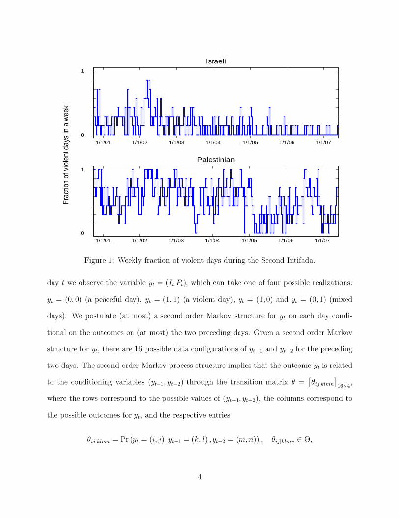
have overwhelmingly been civilian. Figure 1 shows the incidence of violence on both sides
over the period September 29, 2000–May 31, 2007.
Concerns that Israel and the Palestinians were becoming involved in a spiraling cycle of
violence and retaliation led to a wide international effort to put an end to the bloodshed.
Diplomatic efforts included proposals by the Quartet (US, EU, UN, and Russia) and a
number of summits and rounds of negotiation in Egypt, Jordan, and elsewhere. The results
(the Mitchell Report, Tenet Plan, the Road Map, the Geneva Accord of 2003, etc.) were
unanimous in recommending disengagement, either gradual or immediate, as a first step
towards peace negotiations. The notion that a cycle of violence exists and feeds on itself
motivates the first main goal of this paper, namely to examine the importance of conflict
dynamics and whether the data are consistent with persistent and retaliatory (“tit-for-tat”)
behavior.
The evolution of the Second Intifada and the historical events leading to it, against the
backdrop of the wider Arab-Israeli conflict, have been well summarized in Kaufman, Salem,
and Verhoeven (2006) and Milton-Edwards and Hinchcliffe (2003), and news summaries of
the conflict appear regularly in the media. Against this background, several facts about the
Second Intifada can be noted. Importantly, the Second Intifada, unlike the First Intifada of
1987-1990, has been a much more violent and prolonged conflict (the First Intifada claimed
the lives of approximately 1,162 Palestinians and 160 Israelis). In addition, during the course
of the Second Intifada, both sides experienced changes in policies and political leadership on
several occasions. These political sub-periods are given in Table 1. Because of the length of
the conflict and the differences in political regimes, it is less likely that the same dynamic
process applies throughout. Indeed, a casual inspection of Figure 1 shows that the incidence
of violence during the Second Intifada was not uniformly distributed, with several periods of
2
Sub-Period Description1. Oct 1, 2000–Feb 6, 2001 Barak period; Sharon elected Prime Minister2. Feb 7, 2001–Feb 28, 2002 Sharon period before extreme violence3. Mar 1, 2002–Apr 30, 2002 Extreme violence; operation “Defensive Shield”4. May 1, 2002–Jun 30, 2003 Post extreme violence; Palestinian cease-fire5. Jul 1, 2003–Nov 11, 2004 Post Palestinian cease-fire; Arafat dies6. Nov 12, 2004–Jan 4, 2006 Post Arafat; Sharon’s second stroke7. Jan 5, 2006–Jul 11, 2006 Olmert, Hamas governments elected; pre-Lebanon War8. Jul 12, 2006–Aug 14, 2006 Lebanon War9. Aug 15, 2006–Nov 25, 2006 Post-Lebanon War10. Nov 26, 2006–May 31,2007 Israeli-Palestinian truce signed by Abbas and Olmert
Table 1: Sub-periods of interest during the Second Intifada.
exacerbated violence and relative calm intermingled with each other. These considerations
motivate the second main goal of this paper – to formally determine the importance of these
particular policy changes on the occurrence of violence during the Second Intifada.
We approach these two main objectives by considering a number of models with different
dynamic and structural characteristics. By formally comparing these models, we can get a
sense of the relative weights that time series behavior on the one hand, and political change
on the other, have in determining the incidence of violence.
The rest of the paper is organized as follows. Section 2 presents the statistical model
and the framework for model comparison and predictive analysis in this context. Section 3
discusses the data used in the study. Section 4 presents our main results, while Section 5
concludes.
2 Statistical Framework
The occurrence of violence on day t (t = 1, ..., T ) is captured by two binary indicator vari-
ables, It and Pt, where It = 1 if any Israeli deaths occur on day t (It = 0 otherwise), and
similarly, Pt = 1 if any Palestinian deaths occur on day t (Pt = 0 otherwise). Therefore, on
3
1/1/01 1/1/02 1/1/03 1/1/04 1/1/05 1/1/06 1/1/07
0
1 Fr
actio
n of
vio
lent
day
s in
a w
eek
Israeli
1/1/01 1/1/02 1/1/03 1/1/04 1/1/05 1/1/06 1/1/07
0
1
Palestinian
Figure 1: Weekly fraction of violent days during the Second Intifada.
day t we observe the variable yt = (It,Pt), which can take one of four possible realizations:
yt = (0, 0) (a peaceful day), yt = (1, 1) (a violent day), yt = (1, 0) and yt = (0, 1) (mixed
days). We postulate (at most) a second order Markov structure for yt on each day condi-
tional on the outcomes on (at most) the two preceding days. Given a second order Markov
structure for yt, there are 16 possible data configurations of yt−1 and yt−2 for the preceding
two days. The second order Markov process structure implies that the outcome yt is related
to the conditioning variables (yt−1, yt−2) through the transition matrix θ =[θij|klmn
]16×4
,
where the rows correspond to the possible values of (yt−1, yt−2), the columns correspond to
the possible outcomes for yt, and the respective entries
θij|klmn = Pr (yt = (i, j) |yt−1 = (k, l) , yt−2 = (m,n)) , θij|klmn ∈ Θ,
4
give the transition probability of the trajectory (yt−1 = (k, l) , yt−2 = (m, n)) → (yt = (i, j)),
for i, j, k, l, m, n ∈ {0, 1}. In the preceding, the parameter space Θ consists of non-negative
numbers which must sum up to 1 for each row of θ, i.e. since θij|klmn are probabilities, they
must satisfy 0 ≤ θij|klmn ≤ 1 and θ00|klmn + θ10|klmn + θ01|klmn + θ11|klmn = 1 for each of the
trajectories. The Markovian structure is thus a useful conceptualization for our data, which
can alternatively be viewed nonparametrically as consisting of three-day strings taking on
one of 64 possible configurations.
Upon letting y = (y1, ..., yT ) denote all the data, the likelihood function factors as a
product of multinomial likelihood contributions
L(θ; y) =∏
k,l,m,n∈{0,1}
∏
i,j∈{0,1}θ
Tij|klmn
ij|klmn , (1)
where Tij|klmn denotes the number of days in the sample corresponding to the string (yt =
(i, j), yt−1 = (k, l), yt−2 = (m,n)). Further, let θklmn =[θ00|klmn, θ10|klmn, θ01|klmn, θ11|klmn
]
denote the elements in row klmn of θ and let Tklmn =∑
i,j∈{0,1} Tij|klmn be the total number
of days in the sample for which (yt−1 = (k, l), yt−2 = (m,n)).
A convenient family of conjugate priors for θ is a product of independent Dirichlet den-
sities, one for each θklmn:
p(θ) =∏
k,l,m,n∈{0,1}D
(θklmn|µklmn
, τ klmn
)(2)
where the Dirichlet density is given by
D(θklmn|µklmn
, τ klmn
)=
Γ (τ klmn)
∏i,j∈{0,1} Γ
(τ klmnµij|klmn
) ∏
i,j∈{0,1}θ
τklmnµij|klmn
−1
ij|klmn
In (2) the preassigned hyperparameter vectors µklmn
= [µ00|klmn
, µ10|klmn
, µ01|klmn
, µ11|klmn
]′
of positive quantities satisfy∑
i,j∈{0,1} µij|klmn
= 1 and τ klmn > 0 is a scalar controlling the
tightness of the prior beliefs around µklmn
. Loosely speaking, τ klmn is the sample size of a
5
fictitious sample yielding the sample proportion µklmn
. From the properties of the Dirichlet
distribution, we know that the mean of θklmn is µklmn
and the variances and covariances are
V ar(θij|klmn|µklmn, τ klmn) =
µij|klmn
(1− µ
ij|klmn
)
1 + τ klmn
(3)
and
Cov(θij|klmn, θqr|klmn|µklmn, τ klmn) = −
µij|klmn
µqr|klmn
1 + τ klmn
. (4)
In addition, marginal and conditional distributions are also Dirichlet.
Given µklmn
and τ klmn, prior density (2) combines easily with likelihood (1) using Bayes’
Theorem to produce the posterior density
p(θ|y) =∏
k,l,m,n∈{0,1}D(θklmn|µklmn, τ klmn), (5)
which is also a product of independent Dirichlet densities, where
τ klmn = τ klmn + Tklmn,
µij|klmn =τ klmnµ
ij|klmn+ Tklmn
τ klmn
=
(1− τ klmn
τ klmn
)Tij|klmn
Tklmn
+
(τ klmn
τ klmn
)µ
ij|klmn, (6)
µklmn =[µ00|klmn, µ10|klmn, µ01|klmn, µ11|klmn
]′.
Because of the prior independence in (5), the posterior analysis breaks into 16 independent
analyses, one for each row of θ. The posterior mean in (6) is a convex combination of the
prior mean and the sample proportion Tij|klmn/Tklmn (the maximum likelihood estimate).
Posterior variances and covariances of θklmn are similar to (3)–(4) with µij|klmn
and τ klmn
replaced by µij|klmn and τ klmn. Additional features of the distributions used here, as well as
general discussion of the use of conjugate priors in Bayesian analysis, can be found in standard
textbooks such as Zellner (1971), Poirier (1995), and Gelman et al. (2003). Important early
6

work on the estimation of multinomial probabilities in contingency tables includes Good
(1965) and Fienberg and Holland (1973).
Before proceeding, we mention that the model presented above is fairly simple, but
nonetheless appropriate for this setting. Similar models have been used in many fields of
science including climatology and meteorology (e.g. Harrison and Waylen 2000), ecology and
biology (e.g. Wootton 2001), and the health sciences (e.g. Sonnenberg and Beck 1993). We
have confined our attention to this structure for two basic reasons. First, the main benefit of
this model is that it is very clear. Its parameters are directly interpretable and unambiguous,
which is an important consideration when one is trying to uncover basic features of the data
in a case study. The second reason is that dynamic simplicity appeared to be favored by the
model comparison framework to which we turn attention next.
2.1 Model Comparison and Prediction
In the context of the Second Intifada, our objectives are to (i) explore the dynamic charac-
teristics of the process generating the violence and (ii) explore the stability of the process
of violence across political sub-periods. These two issues are formally addressed by compar-
ing several alternative models incorporating different dynamic and structural characteristics,
through their marginal likelihoods and Bayes factors (Jeffreys 1961, Kass and Raftery 1995).
In particular, for any two competing models Mi and Mj, upon using Bayes’ theorem, the
posterior odds can be written as
p (Mi|y)
p (Mj|y)=
p (Mi)
p (Mi)× p (y|Mi)
p (y|Mj), (7)
where the first fraction on the right hand side is known as the prior odds, and the second is
called the Bayes factor. The Bayes factor, in turn, is the ratio of the marginal likelihoods
7
under the two models, where
p (y|Ml) =
∫
Θ
L(θ; y,Ml)p (θ|Ml) dθ, (8)
and where the prior distribution and likelihood function now explicitly involve conditioning
on the model indicator Ml to underscore the dependence of θ on Ml. Importantly, because
of the tractability of the posterior distribution in our setting, the marginal likelihoods are
available analytically as
p(y|Ml) =p(θ|Ml)L(θ; y,Ml)
p(θ|y,Ml)=
∏
k,l,m,n∈{0,1}
Γ (τ klmn)∏
i,j∈{0,1}Γ
(τ klmnµij|klmn
)
Γ (τ klmn)∏
i,j∈{0,1}Γ
(τ klmnµij|klmn
) .
The marginal likelihoods obtained in this way can be used to assess the posterior odds
in (7), or given a set of models {M1, ...,ML} under consideration, one can use the model
probabilities p (Mi|y) for model averaging in predictive inference.
Two additional issues deserve emphasis in this setting. The first is that when comparing
alternative models, the quantities in (7) and (8) should be computed using the same data
y. This is particularly important when considering models with different dynamics and
numbers of lags. Since in our application the largest model contains two lags, the first two
days of the Intifada, September 29-30, 2000, are used as initial observations upon which
all further analysis is conditioned; the effective sample therefore begins with October 1,
2000 (t = 1) and continues through May 31, 2007 (T = 2434). We use the same effective
sample even for models with simpler dynamics (one lag or no lags) because the models being
compared should be fit on the same data. The second issue is that when y is broken up
into, say, J periods y = (y1, ..., yJ), and within each period we allow for a different set
of parameters so that θ = (θ1, ..., θJ), each one independent of the other periods (so that
p (θ|Ml) = p (θ1|Ml) · · · p (θJ |Ml)), the marginal likelihood becomes the product of the
8
sub-period marginal likelihoods
p (y|Ml) =
∫L(θ1; y1,Ml) · · · L(θJ ; yJ ,Ml)p (θ1|Ml) · · · p (θJ |Ml) dθ1 · · · dθJ
=J∏
j=1
∫L(θj; yj,Ml)p (θj|Ml) dθj.
Equivalently, on the log scale ln p (y|Ml) =∑J
j=1 ln p (yj|Ml).
Finally, the one-day ahead posterior predictive mass function for yT+1 given yT and yT−1
is
Pij|klmn = Pr (yT+1 = (i, j) |yT = (k, l) , yT−1 = (m,n))
=
∫ 1
0
θij|klmnp(θij|klmn|y
)dθij|klmn = µklmn,
which is the posterior mean. Hence, appropriate credibility bands for this prediction are
given by (3) with µklmn
replaced by µklmn and τ klmn replaced by τ klmn.
3 Data
We have compiled an up-to-date data set on the Second Intifada from www.btselem.org,
an Israeli human rights organization that is well respected by both sides in the conflict, as
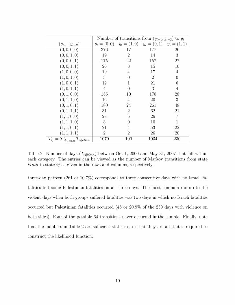
well as by international organizations. From the last line of Table 2 it is seen that out of
the 2434 observations between October 1, 2000 and May 31, 2007, 1070 (44%) correspond
to peaceful days with no fatalities, 100 (4.1%) correspond to days with Israeli fatalities
but no Palestinian fatalities, 1034 (42.4%) correspond to days with no Israeli fatalities but
with Palestinian fatalities, and 230 (9.5%) correspond to violent days with both Israeli and
Palestinian fatalities.
To assess temporal dependence, Table 2 also provides the number of transitions of the
Markov process. The most common pattern (376 or 15.4% of the 2434 observations) corre-
sponds to three consecutive days with no fatalities on either side. The next most common
9
Number of transitions from (yt−1, yt−2) to yt
(yt−1, yt−2) yt = (0, 0) yt = (1, 0) yt = (0, 1) yt = (1, 1)(0, 0, 0, 0) 376 17 177 26(0, 0, 1, 0) 19 2 14 3(0, 0, 0, 1) 175 22 157 27(0, 0, 1, 1) 26 3 15 10(1, 0, 0, 0) 19 4 17 4(1, 0, 1, 0) 3 0 2 0(1, 0, 0, 1) 12 1 21 6(1, 0, 1, 1) 4 0 3 4(0, 1, 0, 0) 155 10 170 28(0, 1, 1, 0) 16 4 20 3(0, 1, 0, 1) 180 24 261 48(0, 1, 1, 1) 31 2 62 21(1, 1, 0, 0) 28 5 26 7(1, 1, 1, 0) 3 0 10 1(1, 1, 0, 1) 21 4 53 22(1, 1, 1, 1) 2 2 26 20
Tij =∑
k,l,m,n Tij|klmn 1070 100 1034 230
Table 2: Number of days (Tij|klmn) between Oct 1, 2000 and May 31, 2007 that fall withineach category. The entries can be viewed as the number of Markov transitions from stateklmn to state ij as given in the rows and columns, respectively.
three-day pattern (261 or 10.7%) corresponds to three consecutive days with no Israeli fa-
talities but some Palestinian fatalities on all three days. The most common run-up to the
violent days when both groups suffered fatalities was two days in which no Israeli fatalities
occurred but Palestinian fatalities occurred (48 or 20.9% of the 230 days with violence on
both sides). Four of the possible 64 transitions never occurred in the sample. Finally, note
that the numbers in Table 2 are sufficient statistics, in that they are all that is required to
construct the likelihood function.
10
4 Analysis
4.1 Choice of Priors
The posterior independence in (5) is quite useful as it aides interpretability and simplifies
the analysis. However, it comes at a price: the need to elicit priors on the rows of θ. In
the two-lag Markov model θ has 16 rows, which implies that 16 vectors µklmn
and 16 scalars
τ klmn should be determined in order to define the prior distributions. In this paper, we assign
common values µij|klmn = 0.25 for the hyperparameters across (i, j, k, l,m, n), implying that
transitions are a priori equiprobable and do not favor any of the alternative outcomes. This
is an important baseline case that is likely to appeal to a wide readership because of its
neutrality on issues such as revenge, preemption, and persistence. To be cautious, however,
we check the effect of this specification on our results by conducting a sensitivity analysis
over three such priors with τ klmn = 2 (Jeffreys’ prior, standard deviations equal to .25),
τ klmn = 4 (uniform prior, standard deviations equal to .1936), and τ klmn = 8 (standard
deviations equal to .1443). When considering no-lag, one-lag, and asymmetric lag models,
the same Dirichlet priors are employed for the rows of θ (the only difference being that θ
will have fewer rows, depending on the model).
4.2 Stability and Dynamics
The time series analysis here addresses two broad issues: correlation over time and stability
over time. The first of these is addressed by introducing lags and the second by allowing
for parameter change; both use up degrees of freedom, particularly the second. Permitting
structural change to take place now implies that the data y can be split into J periods
y = (y′1, ..., y′J)′ and in each of these periods the models and parameters can be different.
While this increases the complexity of the model that explains y (that model consists of
11
Israeli Lags Palestinian Lags0 1 2
0 -2637.21 -2594.59 -2581.361 -2614.34 -2584.37 -2575.232 -2608.44 -2585.70 -2585.04
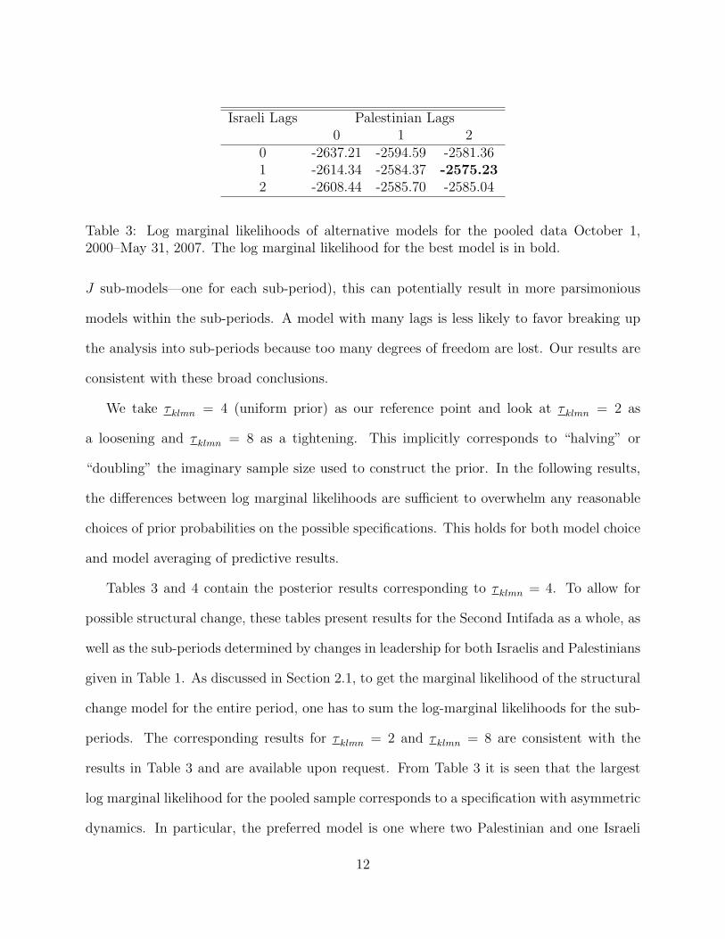
Table 3: Log marginal likelihoods of alternative models for the pooled data October 1,2000–May 31, 2007. The log marginal likelihood for the best model is in bold.
J sub-models—one for each sub-period), this can potentially result in more parsimonious
models within the sub-periods. A model with many lags is less likely to favor breaking up
the analysis into sub-periods because too many degrees of freedom are lost. Our results are
consistent with these broad conclusions.
We take τ klmn = 4 (uniform prior) as our reference point and look at τ klmn = 2 as
a loosening and τ klmn = 8 as a tightening. This implicitly corresponds to “halving” or
“doubling” the imaginary sample size used to construct the prior. In the following results,
the differences between log marginal likelihoods are sufficient to overwhelm any reasonable
choices of prior probabilities on the possible specifications. This holds for both model choice
and model averaging of predictive results.
Tables 3 and 4 contain the posterior results corresponding to τ klmn = 4. To allow for
possible structural change, these tables present results for the Second Intifada as a whole, as
well as the sub-periods determined by changes in leadership for both Israelis and Palestinians
given in Table 1. As discussed in Section 2.1, to get the marginal likelihood of the structural
change model for the entire period, one has to sum the log-marginal likelihoods for the sub-
periods. The corresponding results for τ klmn = 2 and τ klmn = 8 are consistent with the
results in Table 3 and are available upon request. From Table 3 it is seen that the largest
log marginal likelihood for the pooled sample corresponds to a specification with asymmetric
dynamics. In particular, the preferred model is one where two Palestinian and one Israeli
12
Israeli Lags Palestinian Lags0 1 2 0 1 2
Subsample 1 Subsample 20 -158.83 -159.15 -160.43 -480.93 -485.54 -486.931 -159.36 -160.79 -163.47 -485.58 -492.66 -497.262 -163.35 -165.83 -169.61 -488.61 -494.59 -499.10
Subsample 3 Subsample 40 -59.63 -60.59 -62.20 -491.76 -496.28 -504.451 -62.73 -64.01 -65.24 -495.22 -501.83 -509.962 -65.86 -67.54 -68.53 -501.55 -509.02 -520.90
Subsample 5 Subsample 60 -508.91 -513.67 -519.29 -364.71 -359.25 -365.821 -512.13 -519.18 -525.48 -358.74 -356.01 -365.242 -517.15 -527.26 -537.00 -359.75 -361.36 -369.17
Subsample 7 Subsample 80 -158.63 -162.82 -171.74 -33.27 -34.97 -38.351 -161.05 -166.03 -174.87 -34.51 -36.32 -39.632 -163.80 -168.86 -178.11 -35.67 -37.57 -40.78
Subsample 9 Subsample 100 -93.46 -96.28 -101.27 -134.59 -136.20 -144.031 -96.03 -98.64 -103.04 -137.15 -138.93 -146.862 -98.46 -101.74 -106.44 -139.69 -141.62 -149.54
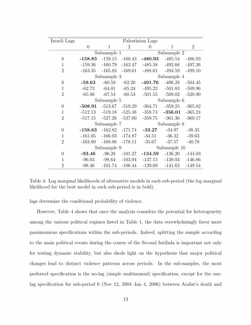
Table 4: Log marginal likelihoods of alternative models in each sub-period (the log marginallikelihood for the best model in each sub-period is in bold).
lags determine the conditional probability of violence.
However, Table 4 shows that once the analysis considers the potential for heterogeneity
among the various political regimes listed in Table 1, the data overwhelmingly favor more
parsimonious specifications within the sub-periods. Indeed, splitting the sample according
to the main political events during the course of the Second Intifada is important not only
for testing dynamic stability, but also sheds light on the hypothesis that major political
changes lead to distinct violence patterns across periods. In the sub-samples, the most
preferred specification is the no-lag (simple multinomial) specification, except for the one-
lag specification for sub-period 6 (Nov 12, 2004–Jan 4, 2006) between Arafat’s death and
13
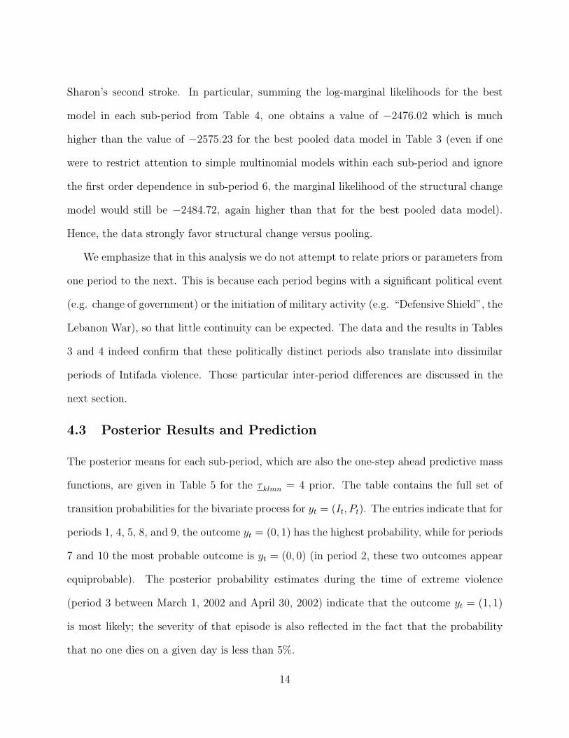
Sharon’s second stroke. In particular, summing the log-marginal likelihoods for the best
model in each sub-period from Table 4, one obtains a value of −2476.02 which is much
higher than the value of −2575.23 for the best pooled data model in Table 3 (even if one
were to restrict attention to simple multinomial models within each sub-period and ignore
the first order dependence in sub-period 6, the marginal likelihood of the structural change
model would still be −2484.72, again higher than that for the best pooled data model).
Hence, the data strongly favor structural change versus pooling.
We emphasize that in this analysis we do not attempt to relate priors or parameters from
one period to the next. This is because each period begins with a significant political event
(e.g. change of government) or the initiation of military activity (e.g. “Defensive Shield”, the
Lebanon War), so that little continuity can be expected. The data and the results in Tables
3 and 4 indeed confirm that these politically distinct periods also translate into dissimilar
periods of Intifada violence. Those particular inter-period differences are discussed in the
next section.
4.3 Posterior Results and Prediction
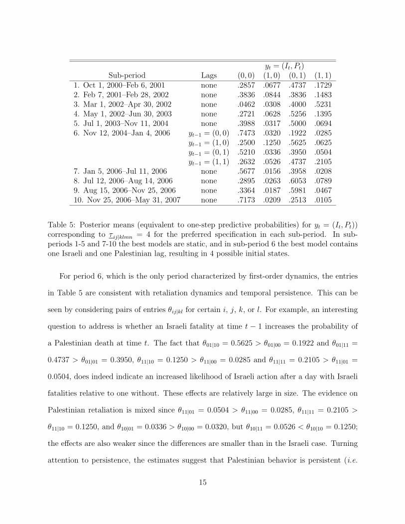
The posterior means for each sub-period, which are also the one-step ahead predictive mass
functions, are given in Table 5 for the τ klmn = 4 prior. The table contains the full set of
transition probabilities for the bivariate process for yt = (It, Pt). The entries indicate that for
periods 1, 4, 5, 8, and 9, the outcome yt = (0, 1) has the highest probability, while for periods
7 and 10 the most probable outcome is yt = (0, 0) (in period 2, these two outcomes appear
equiprobable). The posterior probability estimates during the time of extreme violence
(period 3 between March 1, 2002 and April 30, 2002) indicate that the outcome yt = (1, 1)
is most likely; the severity of that episode is also reflected in the fact that the probability
that no one dies on a given day is less than 5%.
14
yt = (It, Pt)Sub-period Lags (0, 0) (1, 0) (0, 1) (1, 1)
1. Oct 1, 2000–Feb 6, 2001 none .2857 .0677 .4737 .17292. Feb 7, 2001–Feb 28, 2002 none .3836 .0844 .3836 .14833. Mar 1, 2002–Apr 30, 2002 none .0462 .0308 .4000 .52314. May 1, 2002–Jun 30, 2003 none .2721 .0628 .5256 .13955. Jul 1, 2003–Nov 11, 2004 none .3988 .0317 .5000 .06946. Nov 12, 2004–Jan 4, 2006 yt−1 = (0, 0) .7473 .0320 .1922 .0285
yt−1 = (1, 0) .2500 .1250 .5625 .0625yt−1 = (0, 1) .5210 .0336 .3950 .0504yt−1 = (1, 1) .2632 .0526 .4737 .2105
7. Jan 5, 2006–Jul 11, 2006 none .5677 .0156 .3958 .02088. Jul 12, 2006–Aug 14, 2006 none .2895 .0263 .6053 .07899. Aug 15, 2006–Nov 25, 2006 none .3364 .0187 .5981 .046710. Nov 25, 2006–May 31, 2007 none .7173 .0209 .2513 .0105
Table 5: Posterior means (equivalent to one-step predictive probabilities) for yt = (It, Pt))corresponding to τ ij|klmn = 4 for the preferred specification in each sub-period. In sub-periods 1-5 and 7-10 the best models are static, and in sub-period 6 the best model containsone Israeli and one Palestinian lag, resulting in 4 possible initial states.
For period 6, which is the only period characterized by first-order dynamics, the entries
in Table 5 are consistent with retaliation dynamics and temporal persistence. This can be
seen by considering pairs of entries θij|kl for certain i, j, k, or l. For example, an interesting
question to address is whether an Israeli fatality at time t − 1 increases the probability of
a Palestinian death at time t. The fact that θ01|10 = 0.5625 > θ01|00 = 0.1922 and θ01|11 =
0.4737 > θ01|01 = 0.3950, θ11|10 = 0.1250 > θ11|00 = 0.0285 and θ11|11 = 0.2105 > θ11|01 =
0.0504, does indeed indicate an increased likelihood of Israeli action after a day with Israeli
fatalities relative to one without. These effects are relatively large in size. The evidence on
Palestinian retaliation is mixed since θ11|01 = 0.0504 > θ11|00 = 0.0285, θ11|11 = 0.2105 >
θ11|10 = 0.1250, and θ10|01 = 0.0336 > θ10|00 = 0.0320, but θ10|11 = 0.0526 < θ10|10 = 0.1250;
the effects are also weaker since the differences are smaller than in the Israeli case. Turning
attention to persistence, the estimates suggest that Palestinian behavior is persistent (i.e.
15

0 500 1000 1500 20000
0.2
0.4
0.6
0.8
1Po
ster
ior p
roba
bilit
y of
vio
lenc
eIsraeli
0 500 1000 1500 20000
0.2
0.4
0.6
0.8
1
Days since start of the Intifada
Palestinian
Figure 2: Posterior probability of violence on each side during the Intifada sub-periods.
there is a higher probability of an Israeli death at time t given there was an Israeli fatality
at time t − 1), since θ11|10 = 0.1250 > θ11|00 = 0.0285, θ11|11 = 0.2105 > θ11|01 = 0.0504,
θ10|10 = 0.1250 > θ10|00 = 0.0320, and θ10|11 = 0.0526 > θ10|01 = 0.0336. On the other hand,
the evidence of persistence in Israeli behavior (Palestinian deaths) is mixed: θ01|01 = 0.3950 >
θ01|00 = 0.1922, θ11|11 = 0.2105 > θ11|10 = 0.1250, and θ11|01 = 0.0504 > θ11|00 = 0.0285, but
θ01|11 = 0.4737 < θ01|10 = 0.5625. Finally, the steady-state (invariant) distribution of the
Markov process for period 6 is given by (0.6460, 0.0368, 0.2736, 0.0437).
From Table 5 one can also obtain various additional quantities of interest. Two such quan-
tities are the marginal probabilities of violence for each side, Pr (It = 1|·) and Pr (Pt = 1|·),which are obtained by simply summing the columns in the Table where the corresponding
violence indicator equals one. These within-period probabilities are given in Figure 2, and
16
1 2 3 4 50
0.1
0.2
0.3
0.4
0.5
y0 = (I
0,P
0) = (0,0)
Time
Prob
abilit
yPr(I
t=1)
Pr(Pt=1)
1 2 3 4 50
0.1
0.2
0.3
0.4
0.5
y0 = (I
0,P
0) = (0,1)
Time
Prob
abilit
y
Pr(It=1)
Pr(Pt=1)
1 2 3 4 50
0.2
0.4
0.6
0.8
y0 = (I
0,P
0) = (1,0)
Time
Prob
abilit
y
Pr(It=1)
Pr(Pt=1)
1 2 3 4 50
0.2
0.4
0.6
0.8
y0 = (I
0,P
0) = (1,1)
Time
Prob
abilit
y
Pr(It=1)
Pr(Pt=1)
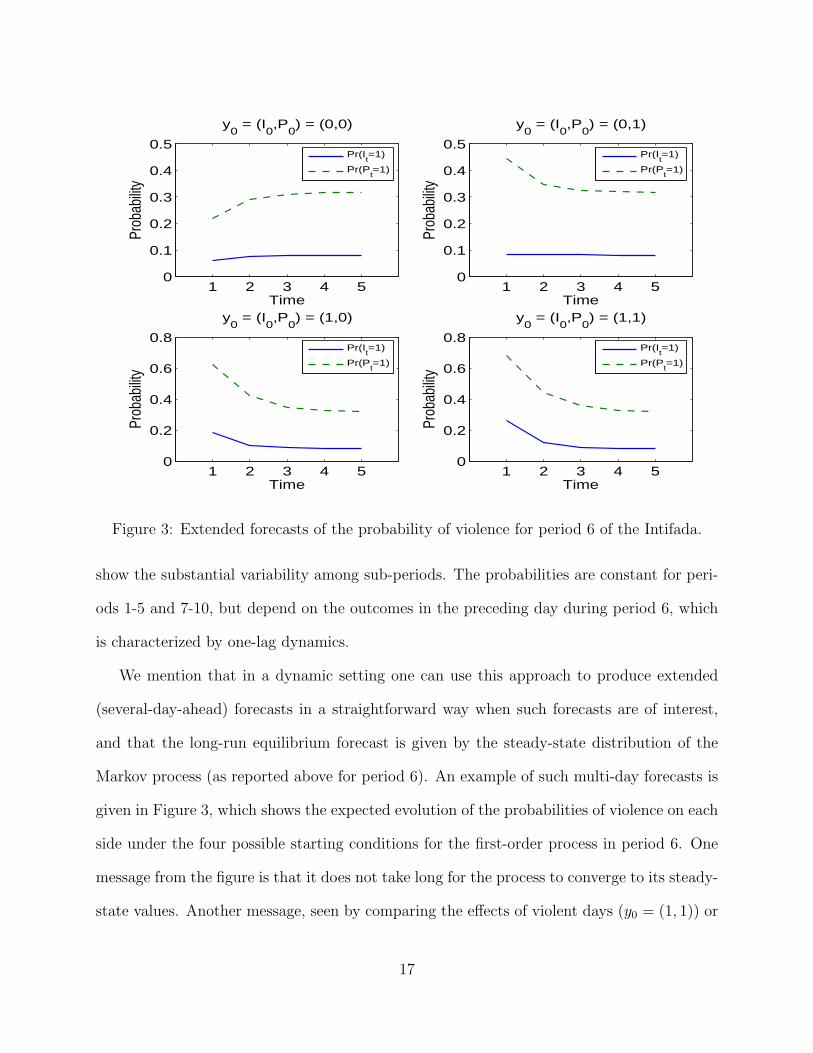
Figure 3: Extended forecasts of the probability of violence for period 6 of the Intifada.
show the substantial variability among sub-periods. The probabilities are constant for peri-
ods 1-5 and 7-10, but depend on the outcomes in the preceding day during period 6, which
is characterized by one-lag dynamics.
We mention that in a dynamic setting one can use this approach to produce extended
(several-day-ahead) forecasts in a straightforward way when such forecasts are of interest,
and that the long-run equilibrium forecast is given by the steady-state distribution of the
Markov process (as reported above for period 6). An example of such multi-day forecasts is
given in Figure 3, which shows the expected evolution of the probabilities of violence on each
side under the four possible starting conditions for the first-order process in period 6. One
message from the figure is that it does not take long for the process to converge to its steady-
state values. Another message, seen by comparing the effects of violent days (y0 = (1, 1)) or
17
mixed days (y0 = (0, 1) or y0 = (1, 0)) to those of peaceful days (yt = (0, 0)), is that violence
on either side raises the prospects of violence for both Israelis and Palestinians in the days
that follow.
5 Conclusion
This paper has analyzed data on the occurrence of violence in the Second Intifada using up-
to-date data series from the conflict. The modelling framework adopted here requires very
little in terms of modelling structure, and hence provides general descriptive characteristics
of the dynamics and structural stability of the process. Our results indicate that the data are
characterized by weak dynamics and strong instability across sub-periods, showing distinct
violence patterns within each political regime. Considering the period October 1, 2000 –
May 31, 2007 as the collection of separate political sub-periods in Table 1, we find robust
evidence of distinct multinomial models over nine of these sub-periods, and a first-order
Markov model for sub-period 6. One implication of this finding is that a fundamental and
credible policy change would appear to offer the best prospects for peace, and that the
dynamics of retaliation and persistence should not be a major impediment in achieving this
goal.
The results of this paper provide ample motivation for further research into the nature of
the conflict and its dynamics and stability. One avenue for research would be to use recent
advances in the estimation of more sophisticated hierarchical models to attempt to capture
the evolution of the probabilities through dynamic latent processes (e.g. Cargnoni et al.
1997, Sung et al. 2007) or through penalties for changes in the probabilities across periods
(Gustafson and Walker 2003). Yet another avenue for research is to consider additional
aspects of the conflict such as data on the intensity of violence, rather than just its occurrence.
18
As a step in this direction, an on-going analysis of the daily death counts is discussed in
Jeliazkov and Poirier (2005).
References
Fienberg, S. E. and P. W. Holland (1973), “Simultaneous Estimation of Multinomial CellProbabilities,” Journal of the American Statistical Association, 68, 683–691.
Gelman, A., J. B. Carlin, H. S. Stern, and D. B. Rubin (2003), Bayesian Data Analysis(2nd edition). New York: Chapman & Hall.
Good, I. J. (1965), The Estimation of Probabilities: An Essay on Modern Bayesian Methods.Cambridge, MA: MIT Press.
Gustafson, P. and L. J. Walker (2003), “An Extension of the Dirichlet Prior for the Analysisof Longitudinal Multinomial Data,” Journal of Applied Statistics, 30, 293–310.
Harrison, M. and P. Waylen (2000), “A Note Concerning the Proper Choice for MarkovModel Order for Daily Precipitation in the Humid Tropics: A Case Study in CostaRica,” International Journal of Climatology, 20, 1861–1872.
Jeffreys, H. (1961), Theory of Probability (3rd edition). Oxford: Clarendon Press.
Jeliazkov, I. and D. J. Poirier (2005), “A statistical model of Intifada fatalities,” UC Irvineworking paper, presented at the Econometric Society World Congress, London, UK.
Kass, R., and A. Raftery (1995), “Bayes Factors,” Journal of the American StatisticalAssociation, 90, 773-795.
Kaufman, E., Salem, W., and J. Verhoeven (editors) (2006), “Bridging the divide: peace-building in the Israeli-Palestinian conflict”. Boulder, Colorado: Lynne Rienner.
Milton-Edwards, B. and P. Hinchcliffe (2004), “Conflicts in the Middle East since 1945,”second edition. New York: Routledge.
Poirier, D. J. (1995), Intermediate Statistics and Econometrics: A Comparative Approach.Cambridge, MA: MIT Press.
Sonnenberg, F. A., and J. R. Beck (1993), “Markov Models in Medical Decision Making:A Practical Guide,”, Medical Decision Making, 13, 322–338.
Sung, M., R. Soyer, and N. Nhan (2007), “Bayesian Analysis of Non-homogeneous MarkovChains: Application to Mental Health Data,” Statistics in Medicine, 26, 3000–3017.
Wootton, J. T. (2001), “Causes of Species Diversity Differences: A Comparative Analysisof Markov Models,” Ecology Letters, 4, 46-56.
19

Zellner, A. (1971), An Introduction to Bayesian Inference in Econometrics. New York:Wiley & Sons.
20