dutch omi no (domino) data product v2 · 4 1 introduction 1.1 purpose and data product this...

1

Dutch OMI NO2 (DOMINO) data product v2.0

HE5 data file user manual

K. F. Boersma, R. Braak, and R. J. van der A

18 August 2011

3

Contents 1. Introduction 2. Overview of the product 3. The data file 4. Remarks on total vs. tropospheric NO2 columns 5. The use of the averaging kernel Appendix Acknowledgments and References Version: 18 August 2011

Abstract

This document provides relevant background information for users interested in improved tropospheric nitrogen dioxide columns from the DOMINO v2.0 retrieval algorithm. It also serves as a manual for using the HDF-EOS5 format DOMINO files. Since October 2004, NO2 retrievals from the Ozone Monitoring Instrument (OMI), a UV/Vis nadir spectrometer onboard NASA’s EOS-Aura satellite, have been used with success in several scientific studies focusing on air quality monitoring, detection of trends, and NOx emission estimates. Dedicated evaluations of DOMINO v1.02 tropospheric NO2 retrievals indicated their good quality, but also suggested that the tropospheric columns were susceptible to high biases (by 0-40%), probably because of errors in the air mass factor calculations. The air mass factor approach for DOMINO v2.0 retrievals has been updated with: 1) a new look-up table (LUT) for altitude-dependent AMFs based on more realistic atmospheric profile parameters, and more surface albedo and surface pressure reference points than before, 2) improved sampling of the TM4 model, resulting in a priori NO2 profiles that are better mixed throughout the boundary layer, 3) a high-resolution terrain height and a high-resolution surface albedo climatology based on OMI measurements, 4) an a posteriori correction for across-track stripes, and 5) extensive flagging for data affected by the so-called row anomalies occurring since June 2007. When using DOMINO v2.0 data, users are advised discard scenes with surface albedo values > 0.3 in addition to the standard TroposphericColumnFlag test.

Front cover figure: summertime mean tropospheric NO2 column in 2005-2008 from OMI for cloud-free situations (cloud radiance fraction <30%) over the Benelux based on the DOMINO v2.0 retrieval. One can clearly recognize (from North to South) the individual hotspots of pollution Rotterdam (NL), Antwerp (BE), the Ruhr Area (G), and Paris (F). Image by Vinken and Boersma et al. [2011].

4

1 Introduction

1.1 Purpose and data product

This document specifies the DOMINO (Dutch OMI NO2) data product, version 2.0. The DOMINO algorithm at KNMI has been updated with respect to version 1.0.2 as described in Boersma et al. [2011]. The main improvements concern:

(1) a more realistic atmospheric (temperature and pressure, i.e. air density) profile for the low atmospheric layers around 1013 hPa (our altitude dependent air mass factors have been calculated with the DAK radiative transfer model using this improved atmospheric profile),

(2) a more realistic, higher spatial resolution terrain height for use in the calculation of the air mass factors,

(3) the consistent use of the OMI-derived surface albedo’s in both the O2-O2 cloud retrieval as well as the NO2 air mass factors, and

(4) an improved sampling of the TM4 a priori NO2 profile shapes resulting in better-mixed NO2 vertical distributions, and

(5) full destriping, and (6) complete row anomaly flagging.

The DOMINO v2.0 algorithm at KNMI has produced a 5+ years (October 2004 – December 2009) set of OMI NO2 data based on Collection 3 level-1b (ir)radiances. The product is available as data and images through www.temis.nl. The Dutch OMI NO2 product is a post-processing data set, based on the most complete set of OMI orbits, improved level-1b (ir)radiance data (collection 3, Dobber et al. [2008]), analysed meteorological fields, and actual spacecraft data. The better data coverage, the improved calibration of level-1b data, and the use of analysed rather than forecast data make the Dutch OMI NO2 product superior to the near-real time NO2 data also available through www.temis.nl (for the time being still retrieved with DOMINO v1). The DOMINO v2.0 product is the recommended product for scientific use, but users can also continue to use DOMINO v1.02 data, that has proven to be useful for scientific studies over the last couple of years (e.g. Hains et al. [2010]; Huijnen et al. [2010], Lamsal et al. [2010], Veefkind et al.

[2011], Zhao et al. [2010]).

1.2 Relation to GOME(-2) and SCIAMACHY NO2 data formats

The GOME, GOME-2, and SCIAMACHY data are available as daily HDF4-files on www.temis.nl. In contrast, Dutch OMI NO2 data are available in the orbital HDF-EOS5 (or HE5) format. The main reason for the transition from HDF4 to HDF-EOS5 is to bring the DOMINO product in line with all other OMI data products that are provided in the HDF-EOS5 format, at the expense of consistency with the GOME and SCIAMACHY heritage. Table 1 summarizes the differences between the HDF4 and HDFEOS5 formats. Table 1. Overview of differences between KNMI satellite NO2 products in the HDF4 and HDF-EOS 5 data formats. HDF4 HDF-EOS 5

GOME(-2), SCIAMACHY OMI v1.0.2 -- OMI v2.0

Daily files Orbital file1

1-dimensional structure (time-ordered, follows satellite ground track)

2-dimensional swath structure (time-ordered and identical to satellite ground track)

1 For consistency with other TEMIS data products, orbital files are provided in a daily tar-file on www.temis.nl.

5

2 Product overview

2.1 DOMINO = Level 2 product

The DOMINO data contains geolocated column integrated NO2 concentrations, or NO2 columns (in units of molecules/cm2). DOMINO data constitute a pure Level 2 product, i.e. it provides geophysical information for each and every ground pixel observed by the instrument, without the additional binning, averaging or gridding typically applied for Level 3 data. In addition to vertical NO2 columns, the product contains intermediate results, such as the result of the spectral fit, fitting diagnostics, assimilated stratospheric NO2 columns, the averaging kernel, cloud information, and error estimates. For advanced users, a second ‘profile’ file is made available that contains geolocated temperature and a priori NO2 profiles at the exact pixel locations. Temperature and NO2 profiles for each and every pixel are not included in the DOMINO product because most users will not need it and we wish to keep the size of the DOMINO files reasonable. Nevertheless, the temperature and NO2 profiles (from the TM4 chemistry-transport model) complete the a priori information used in the retrieval algorithm to compute the stratospheric NO2 columns, the air mass factors, and the temperature correction [Boersma et al., 2007]. This product will be discussed in a separate document.

2.2 Destriping

This document applies to the Dutch OMI NO2 data product, version 2.0. For DOMINO version 1.0.2, we refer to www.temis.nl, where the product specification document for that data version can be downloaded. DOMINO v2.0 uses collection 3 Level 1B data [Dobber et

al., 2008]. Collection 3 Level 1B data are based on much improved instrument calibration parameters that lead to much less across-track variability, or stripes, in the OMI data products compared to pre-Collection 3 level 1B data. Nevertheless, the magnitude of the stripes in v1.0.2 was such that it warranted corrections still. Therefore we have now included a new, a posteriori stripe correction, that reduces much of the stripes, without introducing significant biases in tropospheric NO2 over extended polluted areas. For instance, over extended polluted areas, the average DOMINO tropospheric NO2 columns with and without stripe correction are similar within 0.5%. For a full description of the stripe correction used in v2.0, we refer to Boersma et al. [2011]. Should users be interested in the ‘original’, striped data, they can easily extract this from the data files. Instead of selecting the TroposphericVerticalColumn data product (which has been destriped) from the .he5 file, they can calculate the original tropospheric column as: (SlantColumnAmountNO2-AssimilatedStratosphericSlantColumn)/ AirMassFactorTropospheric.

2.3 Row anomalies

Since June 2007, OMI data are affected by so-called row anomalies. The first row anomaly occurred in June 2007 and stayed constant afterwards. It was followed by a second event in May 2008, and a third in January 2009. During the last two events, the row anomalies showed more dynamic behaviour, with some rows deteriorating, and others that at first appeared affected, veering back to uncompromised states. Since 2009, there have been extended periods during which the row anomaly remained stable, but occasionally subtle changes occurred impredictably.

6

The origin of the row anomalies is unclear at the moment, but there are indications that the OMI field of view is partly obstructed since June 2007. This obstruction has probably caused a number of effects:

a) part of the incoming earthlight is blocked, b) due to inhomogeneous illumination, wavelength shifts occur, c) stray sunlight is reflected into the field-of-view, and d) stray earthshine is reflected into the field-of-view.

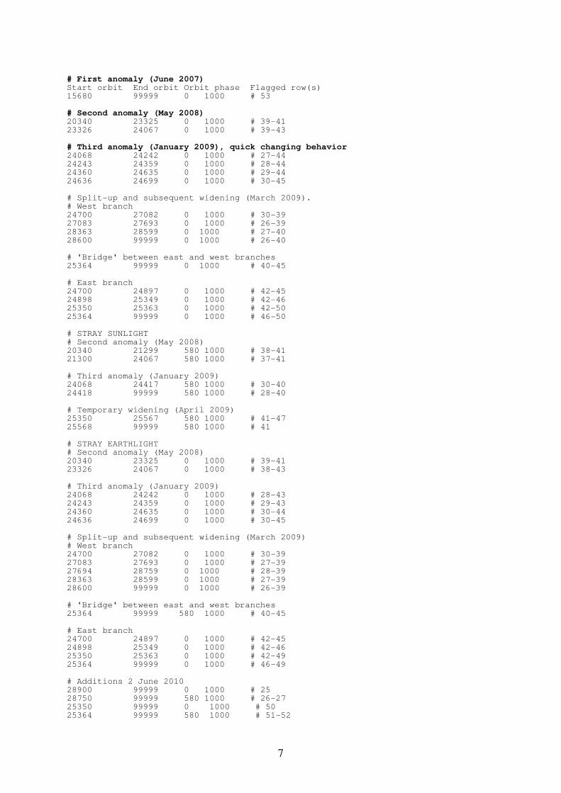
These anomalies have affected the quality of the OMI Level 1B and thereby Level 2 data products. Various row anomaly correction algorithms have been developed since the first occurrence, but to date, no satisfying correction has been implemented that effectively removes the anomalies. Therefore, the DOMINO v2.0 algorithm simply follows the Row Anomaly Flagging Rules [Braak, 2010] and discards the affected rows as not fit for scientific use. These rules specify the most up-to-date knowledge of the (dynamic) occurrence of particular row anomalies. We follow the rules specified for the VIS channel (0-based, i.e. OMI rows run from 0 to 59), which is somewhat different than the rules for the UV-channels (for instance in the VIS channel, only row 53 has been affected, whereas in the UV-channels both 53 and 54 have been affected). Two sorts of row anomalies occur: those that affect the rows along the complete orbit, and those that only occur for part of the orbit, but in practice these anomalies almost always overlap, and it is safe to assume that once a row is affected, it is affected for the complete orbit. Rows can be be affected by the wavelength shift (deteriorating the DOAS NO2 slant column fit), blockage (compromising cloud fraction retrievals), and stray earthlight. In DOMINO v2.0 row anomaly flagging, we follow a conservative approach. If the row anomaly flags are set for whatever reason, we have decided to raise the TroposphericColumnFlag datafield to -1, indicating that the retrieval for that particular pixel is unreliable and should not be used. This implies that we do not distinguish between the various reasons listed above, but simply indicate that the pixel should be discarded. Since orbit 29000 (December 2009), approximately half of the pixels per orbit are compromised. OMI nevertheless continues to provide large quantities useful scientific measurements well after the first row anomalies occurred, as indicated by the daily images provided on www.temis.nl showing that OMI still covers 70-80% of the globe. Below, the simplified contents of the initial version of the row anomaly flagging rules lookup table for the VIS channel is reproduced from Braak [2010]. Data users can verify for themselves that rows past the start orbit should be flagged, and preferably not be used in scientific studies. The name of the original file as it is known in the TMCF is: OMI-Aura_TMCF-OMTDOPFPARM_x1301-xtrackqf_v001-2011m0809t074500.txt. # VISIBLE CHANNEL

7

# First anomaly (June 2007) Start orbit End orbit Orbit phase Flagged row(s) 15680 99999 0 1000 # 53 # Second anomaly (May 2008) 20340 23325 0 1000 # 39-41 23326 24067 0 1000 # 39-43 # Third anomaly (January 2009), quick changing behavior 24068 24242 0 1000 # 27-44 24243 24359 0 1000 # 28-44 24360 24635 0 1000 # 29-44 24636 24699 0 1000 # 30-45 # Split-up and subsequent widening (March 2009). # West branch 24700 27082 0 1000 # 30-39 27083 27693 0 1000 # 26-39 28363 28599 0 1000 # 27-40 28600 99999 0 1000 # 26-40 # 'Bridge' between east and west branches 25364 99999 0 1000 # 40-45 # East branch 24700 24897 0 1000 # 42-45 24898 25349 0 1000 # 42-46 25350 25363 0 1000 # 42-50 25364 99999 0 1000 # 46-50 # STRAY SUNLIGHT # Second anomaly (May 2008) 20340 21299 580 1000 # 38-41 21300 24067 580 1000 # 37-41 # Third anomaly (January 2009) 24068 24417 580 1000 # 30-40 24418 99999 580 1000 # 28-40 # Temporary widening (April 2009) 25350 25567 580 1000 # 41-47 25568 99999 580 1000 # 41 # STRAY EARTHLIGHT # Second anomaly (May 2008) 20340 23325 0 1000 # 39-41 23326 24067 0 1000 # 38-43 # Third anomaly (January 2009) 24068 24242 0 1000 # 28-43 24243 24359 0 1000 # 29-43 24360 24635 0 1000 # 30-44 24636 24699 0 1000 # 30-45 # Split-up and subsequent widening (March 2009) # West branch 24700 27082 0 1000 # 30-39 27083 27693 0 1000 # 27-39 27694 28759 0 1000 # 28-39 28363 28599 0 1000 # 27-39 28600 99999 0 1000 # 26-39 # 'Bridge' between east and west branches 25364 99999 580 1000 # 40-45 # East branch 24700 24897 0 1000 # 42-45 24898 25349 0 1000 # 42-46 25350 25363 0 1000 # 42-49 25364 99999 0 1000 # 46-49 # Additions 2 June 2010 28900 99999 0 1000 # 25 28750 99999 580 1000 # 26-27 25350 99999 0 1000 # 50 25364 99999 580 1000 # 51-52

8

#Changes per PL-OMIE-KNMI-960 Issue 4 (18 May 2011) 35700 99999 0 1000 # 51-52 36100 99999 580 1000 # 25 # Changes per PL-OMIE-KNMI-960 Issue 5 (9 August 2011) 37000 99999 0 1000 # 40 37000 99999 0 1000 # 41-45

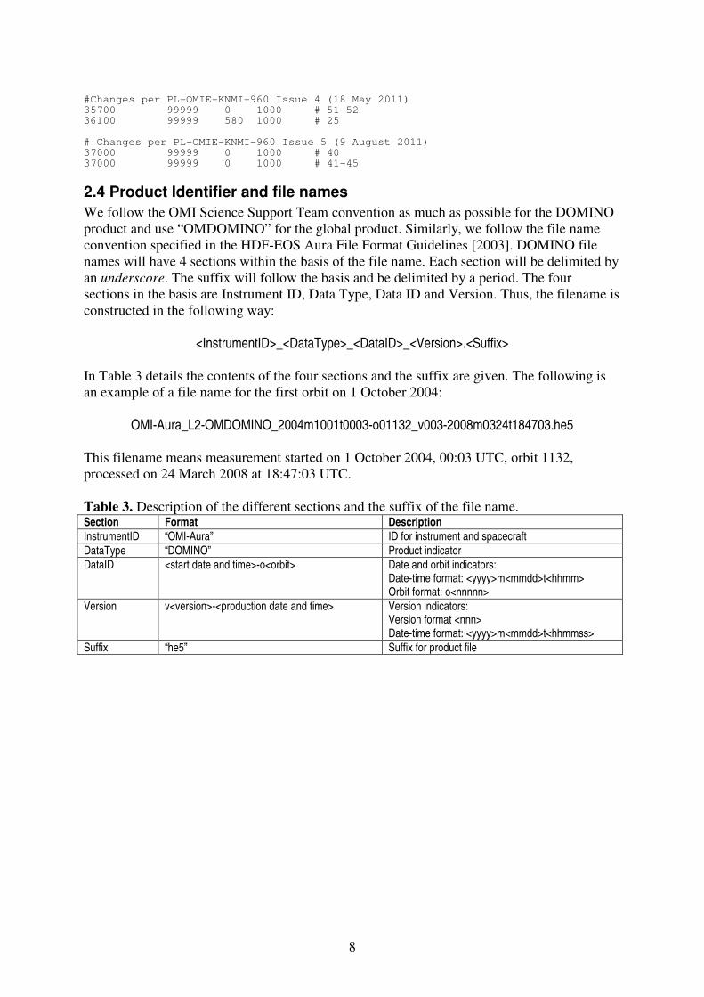
2.4 Product Identifier and file names

We follow the OMI Science Support Team convention as much as possible for the DOMINO product and use “OMDOMINO” for the global product. Similarly, we follow the file name convention specified in the HDF-EOS Aura File Format Guidelines [2003]. DOMINO file names will have 4 sections within the basis of the file name. Each section will be delimited by an underscore. The suffix will follow the basis and be delimited by a period. The four sections in the basis are Instrument ID, Data Type, Data ID and Version. Thus, the filename is constructed in the following way:

<InstrumentID>_<DataType>_<DataID>_<Version>.<Suffix> In Table 3 details the contents of the four sections and the suffix are given. The following is an example of a file name for the first orbit on 1 October 2004:

OMI-Aura_L2-OMDOMINO_2004m1001t0003-o01132_v003-2008m0324t184703.he5 This filename means measurement started on 1 October 2004, 00:03 UTC, orbit 1132, processed on 24 March 2008 at 18:47:03 UTC. Table 3. Description of the different sections and the suffix of the file name. Section Format Description

InstrumentID “OMI-Aura” ID for instrument and spacecraft

DataType “DOMINO” Product indicator

DataID <start date and time>-o<orbit> Date and orbit indicators: Date-time format: <yyyy>m<mmdd>t<hhmm> Orbit format: o<nnnnn>

Version v<version>-<production date and time> Version indicators: Version format <nnn> Date-time format: <yyyy>m<mmdd>t<hhmmss>

Suffix “he5” Suffix for product file

9

3 The Data File

3.1 Description and format

The OMI-Aura_L2-OMDOMINO_<yyyy>m<mmdd>t<hhmm>-o<nnnnn>_v003-<yyyy>m<mmdd>t<hhmmss>.he5 files contain data on NO2 retrieved during one orbit. The format of the data file is HDF-EOS 5. To ease the use of EOS Aura data sets, the Aura teams have agreed to make their files match as closely as possible. To this end, the Aura teams have agreed on a set of guidelines for their file formats, as described in HDF-EOS Aura File Format Guidelines [2003]. The data file uses the HDF-EOS Swath format. Figure 1 shows an example of the structure of a DOMINO data file, when viewed using hdfview. Figure 1. Structure of a DOMINO data file, when opened with hdfview (publicly available through http://hdf.ncsa.uiuc.edu/hdf-java-html/hdfview/ ).

Figure 1 shows that the file contains a single swath structure named “DominoNO2”. This is where all relevant retrieval data are stored. The swath structure consists of Data Fields and Geolocation Fields, but we start with StructMetadata.0, since this holds information on the size of the Data Fields and Geolocation Fields, that is being read in before the Data Fields and Geolocation Fields are read in.

3.2 StructMetadata.0

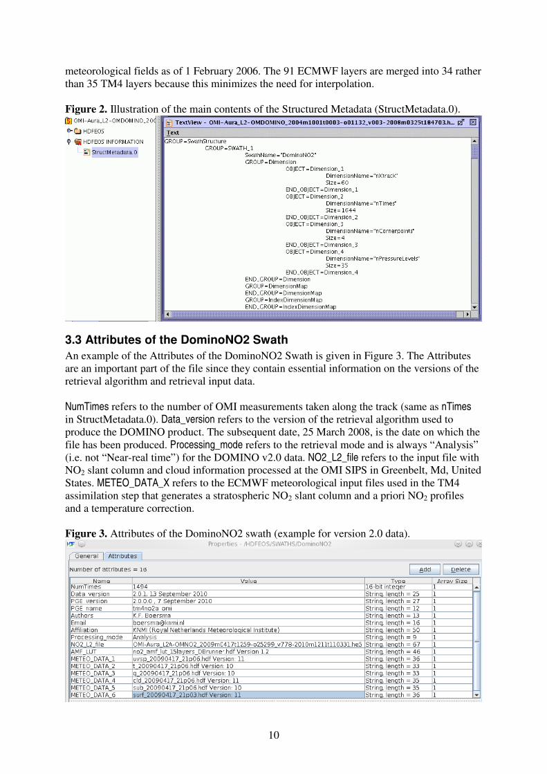
The most important information stored in StructMetadata.0 are the DIMENSIONS. For a DOMINO data file, there are four relevant DIMENSIONS. These pertain to the number of pixels across track (nXtrack), the number of measurements along track (nTimes), the number of corner points that specify the spatial extent of a pixel (nCornerpoints), and the number of pressure levels used in the air mass factor calculation (nPressureLevels). The contents of StructMeadata.0 are illustrated in Figure 2. With the exception of nCornerpoints (always 4), the dimensions may differ between different files. For instance, nXtrack = 60 for nominal-model OMI measurements, but nXtrack = 30 for zoom mode measurements. nTimes is practically always 1644 (corresponding to 1644 2-s measurements along track). nPressureLevels = 35 for the period 1 October 2004 – 31 January 2006, and nPressureLevels = 34 from 1 February 2006 onwards. This change in the number of layers originates from a transition(from 60 to 91 layers) in the operational model ECMWF

10

meteorological fields as of 1 February 2006. The 91 ECMWF layers are merged into 34 rather than 35 TM4 layers because this minimizes the need for interpolation. Figure 2. Illustration of the main contents of the Structured Metadata (StructMetadata.0).

3.3 Attributes of the DominoNO2 Swath

An example of the Attributes of the DominoNO2 Swath is given in Figure 3. The Attributes are an important part of the file since they contain essential information on the versions of the retrieval algorithm and retrieval input data. NumTimes refers to the number of OMI measurements taken along the track (same as nTimes in StructMetadata.0). Data_version refers to the version of the retrieval algorithm used to produce the DOMINO product. The subsequent date, 25 March 2008, is the date on which the file has been produced. Processing_mode refers to the retrieval mode and is always “Analysis” (i.e. not “Near-real time”) for the DOMINO v2.0 data. NO2_L2_file refers to the input file with NO2 slant column and cloud information processed at the OMI SIPS in Greenbelt, Md, United States. METEO_DATA_X refers to the ECMWF meteorological input files used in the TM4 assimilation step that generates a stratospheric NO2 slant column and a priori NO2 profiles and a temperature correction. Figure 3. Attributes of the DominoNO2 swath (example for version 2.0 data).

11

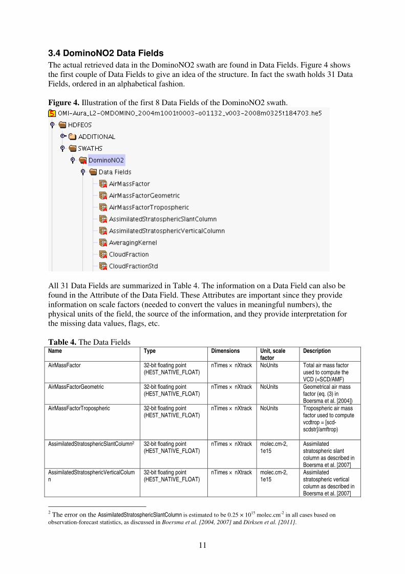
3.4 DominoNO2 Data Fields

The actual retrieved data in the DominoNO2 swath are found in Data Fields. Figure 4 shows the first couple of Data Fields to give an idea of the structure. In fact the swath holds 31 Data Fields, ordered in an alphabetical fashion. Figure 4. Illustration of the first 8 Data Fields of the DominoNO2 swath.

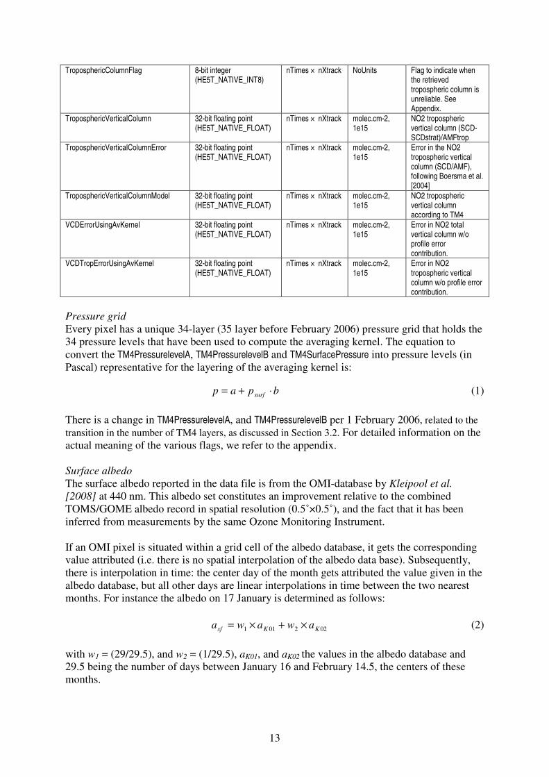
All 31 Data Fields are summarized in Table 4. The information on a Data Field can also be found in the Attribute of the Data Field. These Attributes are important since they provide information on scale factors (needed to convert the values in meaningful numbers), the physical units of the field, the source of the information, and they provide interpretation for the missing data values, flags, etc. Table 4. The Data Fields Name Type Dimensions Unit, scale

factor Description

AirMassFactor 32-bit floating point (HE5T_NATIVE_FLOAT)

nTimes × nXtrack NoUnits Total air mass factor used to compute the VCD (=SCD/AMF)

AirMassFactorGeometric 32-bit floating point (HE5T_NATIVE_FLOAT)

nTimes × nXtrack NoUnits Geometrical air mass factor (eq. (3) in Boersma et al. [2004])

AirMassFactorTropospheric 32-bit floating point (HE5T_NATIVE_FLOAT)

nTimes × nXtrack NoUnits Tropospheric air mass factor used to compute vcdtrop = [scd-scdstr]/amftrop)

AssimilatedStratosphericSlantColumn2 32-bit floating point (HE5T_NATIVE_FLOAT)

nTimes × nXtrack molec.cm-2, 1e15

Assimilated stratospheric slant column as described in Boersma et al. [2007]

AssimilatedStratosphericVerticalColumn

32-bit floating point (HE5T_NATIVE_FLOAT)


Assimilated stratospheric vertical column as described in Boersma et al. [2007]

2 The error on the AssimilatedStratosphericSlantColumn is estimated to be 0.25 × 1015 molec.cm-2 in all cases based on

observation-forecast statistics, as discussed in Boersma et al. [2004, 2007] and Dirksen et al. [2011].

12

AveragingKernel 16-bit integer (HE5T_NATIVE_INT16)

nLayer × nTimes × nXtrack

NoUnits, 0.001 Averaging kernel as described in Eskes and Boersma [2003]

Cloud Fraction 16-bit integer (HE5T_NATIVE_INT16)

nTimes × nXtrack NoUnits, 0.001 Effective cloud fraction as described in Acarreta et al. [2004]

CloudFractionStd 16-bit integer (HE5T_NATIVE_INT16)

nTimes × nXtrack NoUnits, 0.001 Effective cloud fraction precision as described in Acarreta et al. [2004]

CloudPressure 16-bit integer (HE5T_NATIVE_INT16)

nTimes × nXtrack hPa Effective cloud pressure as described in Acarreta et al. [2004]

CloudPressureStd 16-bit integer (HE5T_NATIVE_INT16)

nTimes × nXtrack hPa Effective cloud pressure precision as described in Acarreta et al. [2004]

CloudRadianceFraction 16-bit integer (HE5T_NATIVE_INT16)

nTimes × nXtrack NoUnits (%), 0.01

Cloud radiance fraction, see Eq. (14) in Boersma et al. [2004]

GhostColumn 32-bit floating point (HE5T_NATIVE_FLOAT)


TM4 vertical NO2 column between surface and effective cloud pressure, following the definition in Burrows et al. [1999]

InstrumentConfigurationId 8-bit unsigned character (HE5T_NATIVE_UINT8)

nTimes NoUnit Unique ID for instrument settings in current swath.

MeasurementQualityFlags 8-bit unsigned character (HE5T_NATIVE_UINT8)

nTimes NoUnit Bit level quality flags at measurement level. See Table AX.

SlantColumnAmountNO2 32-bit floating point (HE5T_NATIVE_FLOAT)


NO2 slant column from DOAS fit

SlantColumnAmountNO2Std 32-bit floating point (HE5T_NATIVE_FLOAT)


Precision of NO2 slant column from DOAS fit

SurfaceAlbedo 16-bit integer (HE5T_NATIVE_INT16)

nTimes × nXtrack NoUnits, 0.0001

Surface albedo from Kleipool et al. [2008]. Values hold for 439 nm.

TM4PressurelevelA 32-bit floating point (HE5T_NATIVE_FLOAT)

nLayer Pa Input for TM4 pressure levels, calculated as p = a + p_surf·b

TM4PressurelevelB 32-bit floating point (HE5T_NATIVE_FLOAT)

nLayer NoUnit Input for TM4 pressure levels, calculated as p = a + p_surf·b

TM4SurfacePressure 32-bit floating point (HE5T_NATIVE_FLOAT)

nTimes × nXtrack hPa TM4 surface pressure of the center of the ground pixel, as used in the AMF calculation (following Zhou et al., AMT, 401-416, 2009).

TM4TerrainHeight 16-bit integer (HE5T_NATIVE_INT16)

nTimes × nXtrack M Surface elevation at ground pixel center, corresponding to the TM4 surface pressure

TM4TropoPauseLevel 8-bit unsigned character (HE5T_NATIVE_UINT8)

nTimes × nXtrack NoUnit TM4 level where tropopause occurs

TerrainHeight 16-bit integer (HE5T_NATIVE_INT16)

nTimes × nXtrack M Terrain height at ground pixel center from high-resolution DEM_3KM Earth Science Data Type database.

TotalVerticalColumn 32-bit floating point (HE5T_NATIVE_FLOAT)


NO2 total vertical column (SCD/AMF)

TotalVerticalColumnError 32-bit floating point (HE5T_NATIVE_FLOAT)


Error in the NO2 total vertical column (SCD/AMF), following Boersma et al. [2004]

13

TroposphericColumnFlag 8-bit integer (HE5T_NATIVE_INT8)

nTimes × nXtrack NoUnits Flag to indicate when the retrieved tropospheric column is unreliable. See Appendix.

TroposphericVerticalColumn 32-bit floating point (HE5T_NATIVE_FLOAT)


NO2 tropospheric vertical column (SCD-SCDstrat)/AMFtrop

TroposphericVerticalColumnError 32-bit floating point (HE5T_NATIVE_FLOAT)


Error in the NO2 tropospheric vertical column (SCD/AMF), following Boersma et al. [2004]

TroposphericVerticalColumnModel 32-bit floating point (HE5T_NATIVE_FLOAT)


NO2 tropospheric vertical column according to TM4

VCDErrorUsingAvKernel 32-bit floating point (HE5T_NATIVE_FLOAT)


Error in NO2 total vertical column w/o profile error contribution.

VCDTropErrorUsingAvKernel 32-bit floating point (HE5T_NATIVE_FLOAT)


Error in NO2 tropospheric vertical column w/o profile error contribution.

Pressure grid

Every pixel has a unique 34-layer (35 layer before February 2006) pressure grid that holds the 34 pressure levels that have been used to compute the averaging kernel. The equation to convert the TM4PressurelevelA, TM4PressurelevelB and TM4SurfacePressure into pressure levels (in Pascal) representative for the layering of the averaging kernel is:

bpap surf ⋅+= (1)

There is a change in TM4PressurelevelA, and TM4PressurelevelB per 1 February 2006, related to the

transition in the number of TM4 layers, as discussed in Section 3.2. For detailed information on the actual meaning of the various flags, we refer to the appendix. Surface albedo

The surface albedo reported in the data file is from the OMI-database by Kleipool et al.

[2008] at 440 nm. This albedo set constitutes an improvement relative to the combined TOMS/GOME albedo record in spatial resolution (0.5˚×0.5˚), and the fact that it has been inferred from measurements by the same Ozone Monitoring Instrument. If an OMI pixel is situated within a grid cell of the albedo database, it gets the corresponding value attributed (i.e. there is no spatial interpolation of the albedo data base). Subsequently, there is interpolation in time: the center day of the month gets attributed the value given in the albedo database, but all other days are linear interpolations in time between the two nearest months. For instance the albedo on 17 January is determined as follows:

022011 KKsf awawa ×+×= (2)

with w1 = (29/29.5), and w2 = (1/29.5), aK01, and aK02 the values in the albedo database and 29.5 being the number of days between January 16 and February 14.5, the centers of these months.

14

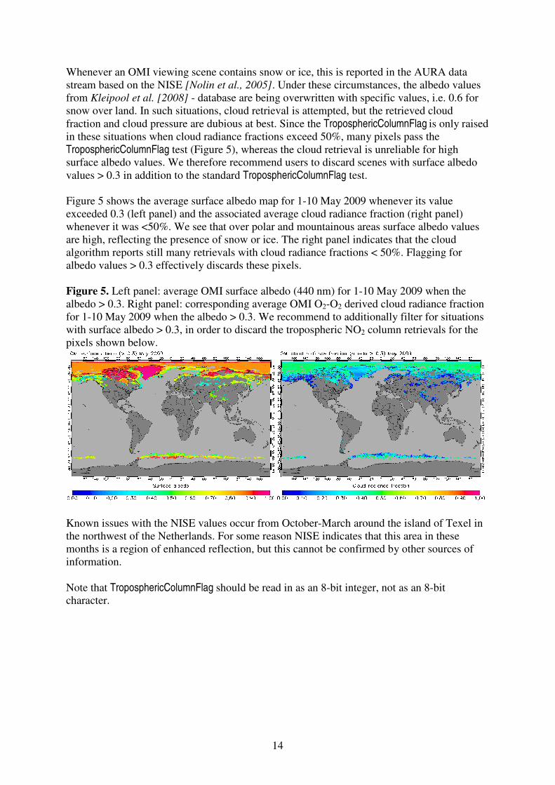
Whenever an OMI viewing scene contains snow or ice, this is reported in the AURA data stream based on the NISE [Nolin et al., 2005]. Under these circumstances, the albedo values from Kleipool et al. [2008] - database are being overwritten with specific values, i.e. 0.6 for snow over land. In such situations, cloud retrieval is attempted, but the retrieved cloud fraction and cloud pressure are dubious at best. Since the TroposphericColumnFlag is only raised in these situations when cloud radiance fractions exceed 50%, many pixels pass the TroposphericColumnFlag test (Figure 5), whereas the cloud retrieval is unreliable for high surface albedo values. We therefore recommend users to discard scenes with surface albedo values > 0.3 in addition to the standard TroposphericColumnFlag test. Figure 5 shows the average surface albedo map for 1-10 May 2009 whenever its value exceeded 0.3 (left panel) and the associated average cloud radiance fraction (right panel) whenever it was <50%. We see that over polar and mountainous areas surface albedo values are high, reflecting the presence of snow or ice. The right panel indicates that the cloud algorithm reports still many retrievals with cloud radiance fractions < 50%. Flagging for albedo values > 0.3 effectively discards these pixels. Figure 5. Left panel: average OMI surface albedo (440 nm) for 1-10 May 2009 when the albedo > 0.3. Right panel: corresponding average OMI O2-O2 derived cloud radiance fraction for 1-10 May 2009 when the albedo > 0.3. We recommend to additionally filter for situations with surface albedo > 0.3, in order to discard the tropospheric NO2 column retrievals for the pixels shown below.

Known issues with the NISE values occur from October-March around the island of Texel in the northwest of the Netherlands. For some reason NISE indicates that this area in these months is a region of enhanced reflection, but this cannot be confirmed by other sources of information. Note that TroposphericColumnFlag should be read in as an 8-bit integer, not as an 8-bit character.

15

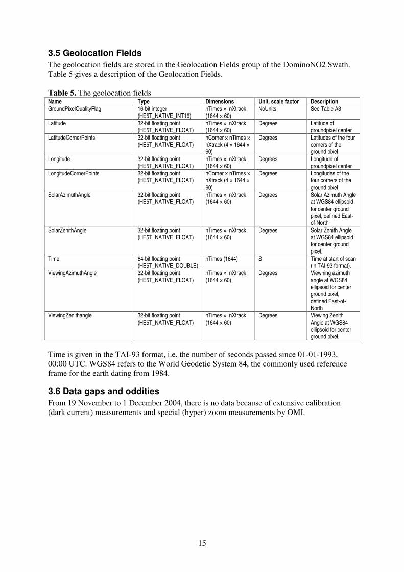
3.5 Geolocation Fields

The geolocation fields are stored in the Geolocation Fields group of the DominoNO2 Swath. Table 5 gives a description of the Geolocation Fields. Table 5. The geolocation fields Name Type Dimensions Unit, scale factor Description

GroundPixelQualityFlag 16-bit integer (HE5T_NATIVE_INT16)

nTimes × nXtrack (1644 × 60)

NoUnits See Table A3

Latitude 32-bit floating point (HE5T_NATIVE_FLOAT)


Degrees Latitude of groundpixel center

LatitudeCornerPoints 32-bit floating point (HE5T_NATIVE_FLOAT)

nCorner × nTimes × nXtrack (4 × 1644 × 60)

Degrees Latitudes of the four corners of the ground pixel

Longitude 32-bit floating point (HE5T_NATIVE_FLOAT)


Degrees Longitude of groundpixel center

LongitudeCornerPoints 32-bit floating point (HE5T_NATIVE_FLOAT)

nCorner × nTimes × nXtrack (4 × 1644 × 60)

Degrees Longitudes of the four corners of the ground pixel

SolarAzimuthAngle 32-bit floating point (HE5T_NATIVE_FLOAT)


Degrees Solar Azimuth Angle at WGS84 ellipsoid for center ground pixel, defined East-of-North

SolarZenithAngle 32-bit floating point (HE5T_NATIVE_FLOAT)


Degrees Solar Zenith Angle at WGS84 ellipsoid for center ground pixel.

Time 64-bit floating point (HE5T_NATIVE_DOUBLE)

nTimes (1644) S Time at start of scan (in TAI-93 format).

ViewingAzimuthAngle 32-bit floating point (HE5T_NATIVE_FLOAT)


Degrees Viewning azimuth angle at WGS84 ellipsoid for center ground pixel, defined East-of-North

ViewingZenithangle 32-bit floating point (HE5T_NATIVE_FLOAT)


Degrees Viewing Zenith Angle at WGS84 ellipsoid for center ground pixel.

Time is given in the TAI-93 format, i.e. the number of seconds passed since 01-01-1993, 00:00 UTC. WGS84 refers to the World Geodetic System 84, the commonly used reference frame for the earth dating from 1984.

3.6 Data gaps and oddities

From 19 November to 1 December 2004, there is no data because of extensive calibration (dark current) measurements and special (hyper) zoom measurements by OMI.

16

4. Remarks on total vs. tropospheric NO2 columns The tropospheric NO2 column is the principal DOMINO product. For historical reasons, an additional total NO2 column is retrieved and stored in the Swath Data Fields. This total NO2 column (TotalVerticalColumn) has been somewhat unfortunately defined as the ratio of the total slant column and the total air mass factor. For users interested in the actual total atmospheric column (integrated from the surface to the top-of-atmosphere), we strongly discourage the scientific use of TotalVerticalColumn. The reason for this is that a total air mass factor is too crude a metric to resolve the intricacies of tropospheric radiative transfer. As a matter of fact, the subtleties involved in accurate radiative transfer for species such as NO2, concentrated in the boundary layer, are the very motivation for retrieval groups to explicitly separate the stratospheric background signal from the slant column before applying a pure tropospheric air mass factor. Therefore, for users interested in the total NO2 column, this quantity should be computed as the sum of the tropospheric and stratospheric vertical columns:

stvtrvv NNN ., += (3)

i.e., by taking the sum of TroposphericVerticalColumn and the AssimilatedStratosphericVerticalColumn.

17

5. The use of the averaging kernel Two distinct user groups can be distinguished: users that take our product ‘face value’, and more advanced users working on extensive scientific projects doing model-to-measurement comparisons and/or satellite validation studies.

(1) Basic users will be mainly interested in the tropospheric column TroposphericVerticalColumn and its error TroposphericVerticalColumnError, and/or the total vertical NO2 column (as defined in Eq. (2)). These users may for instance want to qualitatively check preliminary results of some field experiment with the retrieved NO2 columns.

(2) Advanced users may be interested in the relation between the (modelled or measured) 'true' vertical distribution of NO2 and the retrieved quantity. These users will want to use the averaging kernel that provides the link between (modelled) reality and retrieval (for more details on the averaging kernel, read Eskes and Boersma [2003]. For example, those who are interested in a model – OMI comparison may want to map the modelled NO2 profiles via the averaging kernel to what OMI would retrieve (y is the 'retrieved' quantity) as follows:

xA ⋅=y (4)

with A the averaging kernel, a vector specified at nLayer pressure levels (sections 3.2, 3.4) and x the vertical distribution of NO2 (in partial subcolumns) from a chemistry-transport model (or from collocated validation measurements) at the same nLayer pressure levels. The user thus needs to either convert his or her vertical (subcolumn) NO2 profile to the pressure grid of the averaging kernel in order to construct a vertical column y as would be retrieved by OMI. In principle, a user may also interpolate the averaging kernel vector to the grid of his or her x. However, since the averaging kernel is so sensitive to changes on small spatial scales, for instance due to rapid cloud changes, interpolation of the averaging kernel vector is discouraged. Users will often be interested in the tropospheric NO2 load. For tropospheric retrievals (with y now the tropospheric column), equation (3) reduces to:

troptrop xA ⋅=tropy (5)

with Atrop the averaging kernel for tropospheric retrievals, defined as:

tropAMF

AMF⋅= AA trop (6)

and xtrop the profile shape for tropospheric levels (levels up to level number TM4TropoPauseLevel as specified in the DataField). The pressure at level TM4TropoPauseLevel does not necessarily correspond to the tropopause pressure but rather gives the pressure of the layer in which the tropopause occurs according to the WMO 1985 tropopause criterium. For (tropospheric) applications using the averaging kernel, the error in y will reduce to VCDTropErrorUsingAvKernel since uncertainties on the a priori vertical NO2 profile no longer contribute. A user should be aware that he or she should then no longer use VCDTropError, because this error includes the profile error term that can now be discarded.

18

Appendix The TropColumnFlag is the most important error flag for users interested in the tropospheric NO2 column. The TropColumnFlag is raised (to -1) if more than 50% of the radiance originates from the cloudy part of a scene, or if the scene is compromised because of the occurrence of a row anomaly. Row anomalies occur from 25 June 2007 (see section 2.3). The second important test we recommend to users is to verify if scenes had surface albedo values < 0.3. For scenes with higher surface albedos, due to snow or ice, the quality of the retrieved cloud parameters has not yet been established, and the cloud fraction and cloud radiance fractions are such that they can pass the TropColumnFlag test (see Figure 5). For users interested in other data products than the actually retrieved tropospheric column, the MeasurementQualityFlag (that applies to the slant column fitting), may be of interest. The GroundPixelQualityFlag does not represent an error flag, but merely provides additional information on the viewing scene. Table A1. Definition of the TropColumnFlag. Value Description

0 Tropospheric column for more than 50% determined by observed information.

-1 Tropospheric Column for more than 50% determined by forward model parameter assumptions (cloud radiance fraction > 50%), or row anomaly.

-127 Missing data

One of the DominoNO2 Swath Data Fields is the MeasurementQualityFlag that relates to the slant column fitting. Table A2 summarizes the possible entries and their description. Table A2. Definition of the MeasurementQualityFlags Bit Name Description

0 Measurement Missing Flag Set if all Ground Pixels give Earth Radiance Missing Flag.

1 Measurement Error Flag Set if any of the L1B MeasurementQualityFlags bit 0, 1or 3 are set for the Radiance or for the used Solar product.

2 Measurement Warning Flag Set if any of the L1B MeasurementQualityFlags bit 0, 1, or 3 are set for the Radiance or for the used Solar product.

3 Rebinned Measurement Flag Set if L1B radiance MeasurmentQualityFlags bit 7 is set to 1.

4 4 SAA Flag Set if L1B MeasurmentQualityFlags bit 10 is set to 1, for the Radiance or for the used Solar product

5 Spacecraft Maneuver Flag Set if L1B MeasurmentQualityFlags bit 11 is set to 1, for the Radiance or for the used Solar product

6 Instrument Settings Error Flag The Earth and Solar InstrumentConfigurationIDs are not compatible.

7 Cloud Data Not Synchronized Flag Set if radiance anc cloud data are not synchronized

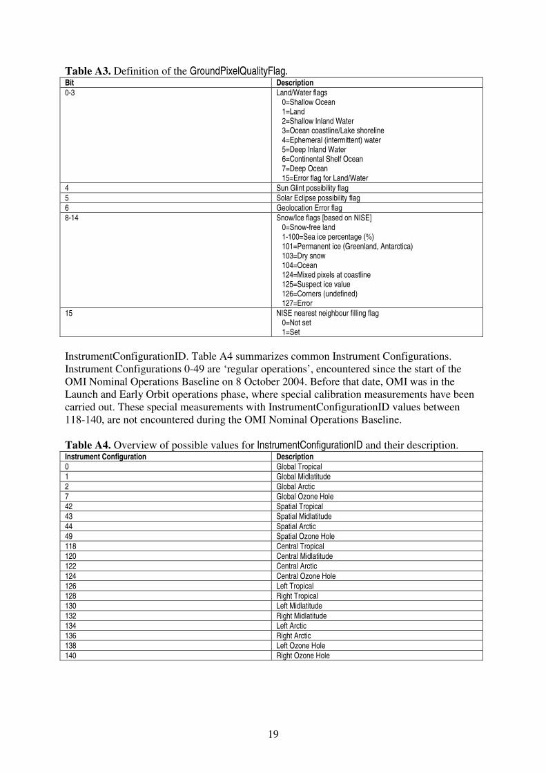
The GroundPixelQualityFlag provides information on the viewing scene. This additional information is stored as a 16-bit integer, whose meaning can be retrieved with dedicated software that will be provided on www.temis.nl. Below are two examples of how the GroundPixelQualityFlag should be interpreted: 65535 = fill value/missing data (all bits have been set) 25857 = Greenland ( 0110 | 0101 | 0000 | 0001 ) Here, bits 0-3 are 0001 representing a numerical value of 1 (20 is set, 21, 22, 23 are not set), i.e. Land. Bits 8-14 are 0110 0101, representing a numerical value of 101 (20+22+25+26=101) i.e. Permanent Ice .

19

Table A3. Definition of the GroundPixelQualityFlag. Bit Description

0-3 Land/Water flags 0=Shallow Ocean 1=Land 2=Shallow Inland Water 3=Ocean coastline/Lake shoreline 4=Ephemeral (intermittent) water 5=Deep Inland Water 6=Continental Shelf Ocean 7=Deep Ocean 15=Error flag for Land/Water

4 Sun Glint possibility flag

5 Solar Eclipse possibility flag

6 Geolocation Error flag

8-14 Snow/Ice flags [based on NISE] 0=Snow-free land 1-100=Sea ice percentage (%) 101=Permanent ice (Greenland, Antarctica) 103=Dry snow 104=Ocean 124=Mixed pixels at coastline 125=Suspect ice value 126=Corners (undefined) 127=Error

15 NISE nearest neighbour filling flag 0=Not set 1=Set

InstrumentConfigurationID. Table A4 summarizes common Instrument Configurations. Instrument Configurations 0-49 are ‘regular operations’, encountered since the start of the OMI Nominal Operations Baseline on 8 October 2004. Before that date, OMI was in the Launch and Early Orbit operations phase, where special calibration measurements have been carried out. These special measurements with InstrumentConfigurationID values between 118-140, are not encountered during the OMI Nominal Operations Baseline. Table A4. Overview of possible values for InstrumentConfigurationID and their description. Instrument Configuration Description

0 Global Tropical

1 Global Midlatitude

2 Global Arctic

7 Global Ozone Hole

42 Spatial Tropical

43 Spatial Midlatitude

44 Spatial Arctic

49 Spatial Ozone Hole

118 Central Tropical

120 Central Midlatitude

122 Central Arctic

124 Central Ozone Hole

126 Left Tropical

128 Right Tropical

130 Left Midlatitude

132 Right Midlatitude

134 Left Arctic

136 Right Arctic

138 Left Ozone Hole

140 Right Ozone Hole

20

Acknowledgments

We are thankful for very useful user feedback provided by Dominik Brunner and Yipin Zhou (EMPA, Switzerland), Jintai Lin (Tsinghua University), Lok Lamsal (Dalhousie University, NASA GSFC), Dylan Millet (University of Minnesota), and Achim Strunk (University of Cologne, Germany).

References Acarreta, J. R., J. F. De Haan, and P. Stammes, Cloud pressure retrieval using the O2-O2 absorption band at 477 nm, J. Geophys. Res., 109, D05204, doi:10.1029/2003JD003915, 2004. Boersma, K. F., H. J. Eskes, and E. J. Brinksma, Error analysis for tropospheric NO2 retrieval from space, J.

Geophys. Res., 109, D04311, doi:10.1029/2003JD003962, 2004. Boersma, K. F., H. J. Eskes, J. P. Veefkind, E. J. Brinksma, R. J. van der A, M. Sneep, G. H. J. van den Oord, P. F. Levelt, P. Stammes, J. F. Gleason, and E. J. Bucsela, Near-real time retrieval of tropospheric NO2 from OMI, Atmos. Chem. Phys., 7, 2103-2118, 2007. Boersma, K. F., D. J. Jacob, E. J. Bucsela, A. E. Perring, R. Dirksen, R. J. van der A, R. M. Yantosca, R. J. Park, M. O. Wenig, T. H. Bertram, and R. C. Cohen, Validation of OMI tropospheric NO2 observations during INTEX-B and application to constrain NOx emissions over the eastern United States and Mexico, Atmos.

Environm., 42(19), 4480-4497, doi:10.1016/j.atmosenv.2008.02.004, 2008. Boersma, K. F., H. J. Eskes, R. J. Dirksen, R. J. van der A, J. P. Veefkind, P. Stammes, V. Huijnen, Q. L. Kleipool, M. Sneep, J. Claas, J. Leitao, A. Richter, Y. Zhou, and D. Brunner, An improved tropospheric NO2 column retrieval algorithm for the Ozone Monitoring Instrument, Atmos. Meas. Tech. Discuss., 4, 2329-2388, doi:10.5194/amtd-4-2329-2011, 2011.

Braak, R., Row Anomaly Flagging Rules Lookup Table, KNMI Technical Document, TN-OMIE-KNMI-950, Issue 1, 12 March 2010. Burrows, J. P., et al., The Global Ozone Monitoring Experiment (GOME): Mission concept and first scientific results, J. Atmos. Sci., 56, 151-175, 1999. Dobber, M., Q. Kleipool, R. Dirksen, P. Levelt, G. Jaross, S. Taylor, T. Kelly, L. Flynn, G. Leppelmeier, and N. Rozemeijer, Validation of Ozone Monitoring Instrument level-1b data products, J. Geophys. Res., 113, D15S06, doi:10.1029/2007JD008665, 2008. Dirksen, R. J., K. F. Boersma, H. J. Eskes, D. V. Ionov, E. J. Bucsela, P. F. Levelt, and H. M. Kelder, Evaluation of stratospheric NO2 retrieved from the Ozone Monitoring Instrument: intercomparison, diurnal cycle and trending, J. Geophys. Res., 116, D08305, doi:10.1029/2010JD014943, 2011. Eskes, H. J., and K. F. Boersma, Averaging kernels for DOAS total-column satellite retrievals, Atmos. Chem.

Phys., 3, 1285-1291, 2003. HDF-EOS Aura File Format Guidelines, NCAR SW-NCA-079, Version 1.3, 27 August 2003. Hains, J. C., Boersma, K. F., Kroon, M., Dirksen, R., Cohen, R., et al.: Testing and improving OMI DOMINO tropospheric NO2 using observations from the DANDELIONS and INTEX-B validation campaigns, J. Geophys.

Res., 115, D05301, doi:10.1029/2009JD0012399, 2010. Huijnen, V., Eskes, H. J., Poupkou, A., Elbern, H., Boersma, K. F.: Comparison of OMI NO2 tropospheric columns with an ensemble of global and European regional air quality models, Atmos. Chem. Phys., 10, 840 3273-3296, 2010. http://www.atmos-chem-phys.net/10/3273/2010/, 2010.

Kleipool, Q.L., M.R. Dobber, J.F. de Haan and P.F. Levelt, Earth surface reflectance climatology from 3 years of OMI data, J. Geophys. Res., 2008, 113, doi:10.1029/2008JD010290, 2008.

21

Lamsal, L. N., Martin, R. V., van Donkelaar, A., Celarier, E. A., Bucsela, E. J., Boersma, K. F., Dirksen, R., Luo, C., and Wang, Y.: Indirect validation of tropospheric nitrogen dioxide retrieved from the Ozone Monitoring Instrument: Insight into the seasonal variation of nitrogen oxides at northern midlatitudes, J. Geophys. Res., 115, D05301, doi:10.1029/2009JD012399, 2010. Lin, J.-T., M. McElroy, and K. F. Boersma, Constraint on anthropogenic NOx emissions in China from different sectors: a new methodology using multiple satellite retrievals, Atmos. Chem. Phys., 10, 63-78. Nolin, A., R. Armstrong, and J. Maslanik, Near-real time SSM/I EASE grid daily global ice concentration and snow extent, Boulder, CO, USA: National Snow and Ice Data Center. Digital Media, 2005, updated daily. Veefkind, J. P., Boersma, K. F., Wang, J., Kurosu, T., Krotkov, N., and Levelt, P. F.: Global analysis of the relation between aerosols and short-lived trace gases, Atmos. Chem. Phys., 11, 1255-1267, 2011. Zhao, C., and Wang, Y.: Assimilated inversion of NOx emissions over east Asia using OMI NO2 column measurements, Geophys. Res. Lett., 36, L06805, doi:10.1029/2008GL037123. Zhou, Y., D. Brunner, K. F. Boersma, R. Dirksen, and P. Wang, An improved tropospheric NO2 retrieval for satellite observations in the vicinity of mountainous terrain, Atmos. Meas. Tech., 2, 401-416, 2009. Zhou, Y., D. Brunner, R. J. D. Spurr, K. F. Boersma, M. Sneep, C. Popp, and B. Buchmann, Accounting for surface reflectance anisotropy in satellite retrievals of tropospheric NO2, Atmos. Meas. Tech., 3, 1185-1203, 2010.

dutch omi no (domino) data product v2 · 4 1 introduction 1.1 purpose and data product this...

Documents