durham e-theses the implementation of a fabrication cell
TRANSCRIPT

Durham E-Theses
The implementation of a fabrication cell and the
optimisation of a pull system with a decision support
system
Panagiotakou, Ellie
How to cite:
Panagiotakou, Ellie (1994) The implementation of a fabrication cell and the optimisation of a pull system
with a decision support system, Durham theses, Durham University. Available at Durham E-Theses Online:http://etheses.dur.ac.uk/5554/
Use policy
The full-text may be used and/or reproduced, and given to third parties in any format or medium, without prior permission orcharge, for personal research or study, educational, or not-for-pro�t purposes provided that:
• a full bibliographic reference is made to the original source
• a link is made to the metadata record in Durham E-Theses
• the full-text is not changed in any way
The full-text must not be sold in any format or medium without the formal permission of the copyright holders.
Please consult the full Durham E-Theses policy for further details.

Academic Support O�ce, Durham University, University O�ce, Old Elvet, Durham DH1 3HPe-mail: [email protected] Tel: +44 0191 334 6107
http://etheses.dur.ac.uk
2

The copyright of this thesis rests with the author.
No quotation from it should be published without
his prior written consent and information derived
from it should be acknowledged.
T H E IMPLEMENTATION OF A FABRICATION CELL AND THE OPTIMISATION OF A PULL
SYSTEM WITH A DECISION SUPPORT SYSTEM
by
E L L I E PANAGIOTAKOU
UNIVERSITY OF DURHAM
1991-1994
This thesis is submitted to fulfil the requirements of a Masters of Science degree
at the University of Durham,
School of Engineering and Computer Science.

ACKNOWLEDGEMENTS
I would like to thank:
My parents for their financial and emotional support during the whole period of my
studies, making it feasible for me to complete this research.
My supervisor, Dr Paul G. Maropoulos, for the valuable guidance during the progress
of this research, for his help and support.
Reyrolle Switchgear Ltd., for providing the data to conduct the research, and the
excellent co-operation of every employee of the company, I would like to refer
especially to Mr Hugh Knox Production Manager, for his support assistance, and
guidance in order to complete this research, additionally I would like to thank Mr
Man Lay Production Engineering Manager, and Ms Kate Strain Industrial
Engineering Manager.
Dr Andrew Farell, and Dr John T. Davies for their assistance in writing up this thesis,
and their support for the duration of this research.
Prof Peter B. Atwell for his invaluable help and guidance.
Final]}' I would like to thank Dr Costas Spanomanolis, who made it possible for me to
start this research, for liis support, assistance and guidance for the duration of the
project.

ABSTRACT
Manufacturing Resource Planning (MRPII) systems are used by forty per cent of UK
manufacturing companies (Little, 1990). In cases where the implementation of the
system was successful the companies have experienced reductions in inventories and
lead times but the results were not always as good as they were anticipated. The
justification of the major capital expenditure that is required for the implementation of
the MRPn system was not always achieved by the benefits gained. Meanwhile, Just in
Time (JTI) manufacturing environments experience benefits in terms of rapid stock-
turns, due-date compliance and quality that MRPII users could not resist.
This research initially focused on the investigation of the reasons of failure of MRPII
implementations in low volume high variety manufacturing environments. The main
reason being that the implementation of the MRPII system was not complemented by
a shop floor re-organisation.
The thesis reports an investigation and some elements of implementation of a change
in the manufacturing operations of a company.
The manufacturing environment that was used for this investigation was ReyroUe
Switchgear Ltd. The production control system used by the company is MRPII,
however, the implementation of the system was not as successful as it was anticipated.
In order to cope with excessive stock, management decided to introduce a pull system
for controlling the production of a limited number of components. The application of
the pull system was Umited because of the complexity in controlling the response of
the manufacturing facilities, which had a functional layout.
/
In order to establish an effective pull system, cellular manufacturing was introduced.
The methodology used was "Line Analysis" which is a sub technique of "Production
m

Flow Analysis". The pull system was complemented by a Decision Support computer
based system in order to facilitate and enhance planning and inventory control.
The changes were implemented and considerable improvements were achieved. The
candidate is a researcher/investigator partly promoting the changes reported,
implementing methods and investigating their effect.
rv

CONTENTS
C H A P T E R 1: P R O D U C T I O N C O N T R O L S Y S T E M S .
1.1. I N T R O D U C T I O N .
1.2. J U S T - D V - T I M E . ,
1.3. M A N U F A C T U R I N G R E S O U R C E P L A N N I N G
1.4. O P T I M I S E D P R O D U C T I O N T E C H N O L O G Y .
1.5 D I S C U S S I O N . .11
1.5.1. JUST-IN-TIME., .11
1.5.2 MANUFACTURING RESOURCE PLANNING.. - - . .12
1.5.3. OPTIMISED PRODUCTION TECHNOLOGY.. .13
C H A P T E R 2. P R O D U C T I O N C O N T R O L A N D F A C T O R Y L A Y O U T . . .15
2.1. T H E M R P I I C H A N G E . .16
2.2. C E L L U L A R M A N U F A C T U R I N G A N D G R O U P T E C H N O L O G Y . .17
2.3. P R O D U C T I O N F L O W A N . \ L Y S I S . .19
2.3.1. F A C T O R Y F L O W A N A L Y S I S . .19
2.3.2. L I N E A N A L Y S I S . . .—;...20
2.4. L I N K B E T W E E N L A Y O U T A N D P R O D U C T I O N C O N T R O L . .21

C H A P T E R 3. U N D E R S T A N D I N G T H E E V D U S T R U L E N V I R O N M E N T . .23
3.1. T H E P R O D U C T S . .23
3.2. M E D I U M V O L T A G E P R O D U C T S , .24
3.2,1. L M T S W I T C H G E A R : 24
3.2.2. L S R S W I T C H G E A R : .25
3.2.3. Y M V S W I T C H G E A R : .25
3.2.4. S M S S W I T C H G E A R : 25
3.2.5. R O S W I T C H G E A R : . , .26
3.2.6. E S R S W I T C H G E A R : . .27
3.3. H I G H V O L T A G E P R O D U C T S . .27
3.4. T H E P R O D U C T I O N C O N T R O L S Y S T E M . 27
3.5. O R D E R I N T A K E . .28
3.6. D E M A N D M A N A G E M E N T . 28
3.7. M A T E R I A L R E Q U I R E M E N T S P L A N N I N G . 29
3.8. S H O P F L O O R . .30
3.8.1. M A C H I N E S H O P . 30
3.8.2. F A B R I C A T I O N S H O P . / .30
3.8.3. A S S E M B L Y S H O P . 31
vi

3.9. S H O P F L O O R O R G A N I S A T I O N
3.10. S H O P F L O O R C O N T R O L
3.11. D I S C U S S I O N
C H A P T E R 4. A C O M P O N E N T B A S E D C E L L
4.1. T H E S H E E T M E T A L S H O P „
4.2. D A T A C O L L E C T I O N „
4.2.1. E X I S T I N G M A T E R I A L F L O W
4.2.2. S I M P L I F I C A T I O N O F T H E M A T E R I A L F L O W
4.2.3. F R O M - T O A N A L Y S I S
4.3. D Y N A M I C P R O G R A M M I N G
4.3.1. T H E T R A V E L L I N G S A L E S M A N P R O B L E M
4.3.2. T H E D E F I N I T I O N A N D S O L U T I O N O F T H E P R O B L E M 49
4.4. P R I O R I T Y A N D M A T E R I A L F L O W R U L E S . . . . .
4.5. F E E D B A C K T O M R F I I
C H A P T E R 5. T H E D E C I S I O N S U P P O R T S Y S T E M
5.1. E X P E R T S Y S T E M S
5.2. C R Y S T A L 4.5
58
vu
/
32
32
34
36
36
37
37
40
™.44
48
- 4 8
51
53
.54
.56
57

5.3. T H E D E C I S I O N S U P P O R T S Y S T E M ' S O B J E C T I V E S .
5.4. T H E D E S C R I P T I O N O F T H E S Y S T E M
5.4.1. T H E D A T A B A S E
5.4.2. T H E E X P E R T S Y S T E M
5.4.3. A D D A J P D A T E O R D E R S
5.4.4. J O B S T O B E S T A R T E D
.59
.61
.61
.63
.63
.67
5.4.5. O R D E R S R E L E A S E / R E C E I P T F R O M T H E F A B R I C A T I O N
S H O P 68
5.4.6. U N E X P E C T E D I N V E N T O R Y R E P L E N I S H M E N T . .
5.4.7. C L O S E O R D E R S
5 3 . I N T E G R A T I N G T H E S Y S T E M
C H A P T E R 6. D I S C U S S I O N A N D C O N C L U S I O N S
APPENDICES
A P P E N D I X I . D A T A C O L L E C T I O N
A P P E N D I X I I . I N S T A L L A T I O N O F T H E S Y S T E M
A P P E N D I X I I I . T H E S O U R C E C O D E F O R T H E D E C I S I O N S U P P O R T
S Y S T E M
.68
.68
.68
...79
.82
viu

FIGURES
FIGURE 4.1. FROM-TO ANALYSIS CHART . .39
40
FJGVRE 4.2 THE SCHEMATIC DIAGRAM OF THE MATERIAL ILOW AT THE
LIGHT FABRICATION SHOP**********>**«»**<*« ••••••••••••••••••••*•*•••••••••<*••*•••*••••«•••.•»«•••••*••••
FIGURE 4.3. FIRST PASS FOR THE IDENTIFICATION OF THE SIMPLIFIED
ROUTINGS - „ 42
FIGURE 4.4. SCHEMATIC DIAGRAM OF THE SIMPUFIED ROUTINGS 43
FIGURE 4.5. THE GENERIC ROUTING IDENTIFIED FOR THE UGHT FABRICATION
SHOP 43
FIGURE 4.6. FROM TO MATRIX BEFORE THE UNE ANALYSIS 47
FIGURE 4.7. FROM TO MATRIX AFTER THE LINE ANALYSIS 47
FIGURE 5.1. T H E PLANNING PROCEDURES OF THE DECISION SUPPORT SYSTEM „.... 60
FIGVRE 5.2. THE STRUCTURE OF THE DATABASE 70
FIGURE 5.3. T H E ASSEMBLY ORDERS FILE ~ „. 61
FIGURE 5.4. THE INVENTORY FILE - ~ - 6 2
FIGURE 5.5. THE FABRICATION ORDERS FILE — 62
FIGURE 5.6. THE MAIN MENU OF THE DECISION SUPPORT SYSTEM - 71
FIGURE S. 7. T H E STRUCTURE OF THE ' A D D A J P D A T E ' MODULE — — . — 7 2
FIGURE .S.8. T H E INPUT SCREEN FOR THE ASSEMBLY ORDERS m£ 73
ix

FIGURE 5.9. THE MESSAGE THAT THE USER GETS WHEN THERE IS NOT
ENOUGH TIME FOR PRODUCTION... " 73
FiGUR£ 5.10. CHANGES THAT CAN BE PERFORMED TO THE DATA HELD BY THE
DATABASE - - 66
FlGUSB 5.11. T H E STRUCTURE OF THE ' J O B S T O B E S T A R T E D * MODULE 74
FIGURE 5.12. T H E OITTUT SCREEN WHICH INCLUDES ALL THE ORDERS THAT
SHOULD START ON A SPECIFIC DAY ~. . ..." 74
.75
FIGURE 5.13. THE OUTPUT SCREEN WHEN NO ORDERS WERE PLANNED TO
START ON A SPECIFIC D A Y . „ •
FIGURE 5.14. T H E STRUCTURE OF THE ' F A B R I C A T I O N O R D E R S F I L E '
MODULE ,.„„•„•«...».••«•••.•».••..•*••••••••••••••••••••••••••••••••••»•••••••»**•••••••• ••••*••••
FIGURE 5.17. THE INPUT SCREEN FOR THE im-ENTORY RECEIVED
UNEXPECTEDLY " •
FIGURE 5.19. T H E INPUT SCREEN TO UPDATE THE SYSTEM ABOUT WHICH
ORDERS ARE COMPLETED — •
.76
FIGURE 5.15. THE OUTPUT SCREEN FOR THE NUMBER OF ORDERS THAT
SHOULD BE RELEASED ON A SPECmC DAY , 76
FIGURE 5.16. T H E STRUCTURE OF THE ' U N E X P E C T E D I N V E N T O R Y
R E P L E N I S H M E N T ' MODULE 77
.77
FIGURE 5.18. T H E STRUCTURE OF THE ' C L O S E O R D E R S ' M O D U L E »~ 78
.78

To my father
and
the beloved memory of my mother
XI

CHAPTER 1, PRODUCTION CONTROL SYSTEMS
1.1. INTRODUCTION
A manufacturing system is a configuration of resources combined for the provision of
goods. The resources are machines, materials used and labour. The objective of any
manufacturing system is to "make money". Therefore, the resources have to be co
ordinated so that the operating cost is minimised, while delivering the products on
time and at the quality requested.
Operations management is concerned with the design and operation of a
manufacturing system. Various methods have been developed for inventoiy control,
scheduling, production planning, capacity planning and machines layout arrangement.
These aspects of management are crucial to the effective and efficient operation of a
manufacturing system. All the aforementioned activities have to co-exist in a given
manufacturing system and also co-ordinated in order to meet the objectives of the
business. The co-ordination is achieved by the production control system used by the
company. The production control system translates the business objectives into day-
to-day targets and activities.
In this first chapter, three contemporary production control systems will be discussed
Just-in-time, Manufacturing Resource Planning and Optimised Production
Technology.

1.2. JUST-IN-TIME
The Just-in-Time (JIT) production control system is presented first, because it is the
control system that has set the targets in many manufacturing environments.
The philosophy that supports a JIT production control system acknowledges the
desire to eliminate all forms of waste in a manufacturing environment. Waste, is
anything that adds cost but no value to the product. Non value adding (NVA)
parameters are stock, work-in-progress (WIP), queues, transportation, set-up times,
scrap, rework, machine breakdown, inspection and material handling (Cheng, 1991;
Japanese Management Association (JMA), 1985; Hall, 1981, 1983, 1987; Shingo,
1985, 1986, 1989).
The JIT philosophy and production control system evolved after forty years of
continuous improvement by Toyota. The management of the company realised at the
end of the 40's, that in order to survive, they had to catch up with American
automotive companies. Through the years the employees and management worked
together to achieve what now is considered to be the best practice in manufacturing
(HaU, 1981, 1983, 1987).
The objective in a JIT environment is to deliver the product(s) on time, at the exact
quantity and quality required. It aims to stockless production, everything produced to
an order.
Timing and accuracy in a JIT environment are of crucial importance. Deficiency can
only result in inventory increase, therefore quality is the cornerstone for a JIT
environment. The three enemies of total quality complexity, variation and attitude,
are tackled at every stage of the manufacturing system .
At source: raw material and components, through integrated customer-supplier relationships, mistake-proofing Poka-Yoke systems of inspection (Shingo, 1985, 1986, 1989), and preventive machine maintenance. At design:

design the product to be right first time. In process: through process control, Statistical Process Control (SPC) which measures the variation within a process (Feigenboum, 1986). In people: distributed responsibility on the shop-floor for quality, and enhanced teamwork (Jewitt, 1990).
Total quality management is implemented throughout all the activities within a
company.
Generally, JIT is characterised by simple and visible systems. Control is conducted
through posted schedules, charts, boards and signal lights which display all the
information required. The visibility and simplicity enhances the accuracy of the data ^
concerning production.
In order to achieve zero inventories the batch sizes are kept to a minimum. This
contributes to the reduction of lead times, as a direct reduction of the machine, and
queuing time required. However issues emerge, which are related to set up time
requirements and quality. A number of optimisation techniques have been developed
so that the benefits fi^om the reduced batch size can be realised (Hall, 1981, 1983,
1987; Shingo, 1985, 1986, 1989).
The organisation of the shop floor is vital to effective control and the establishment
of simplicity and visibility. In a JIT environment the arrangement of machines is based
on the product requirements rather than the functionality of the machines. Groups of
machines are brought together to manufacture a product or a range of similar
components. The arrangement of machines is U-shaped, C-shaped or there is a linear
arrangement in order to minimise the travelling distance and allow close contact
between the operators. Next to the machines there are clearly identified input, and
output areas. The input area is for the components to be processed, whereas the
output area is for those components that have already been processed by the
machine. This organisation of the shop floor enhances visibility with respect to
material flow and problems that might occur can be identified easily. Additional
measures concerning the material flow are taken in order to prevent the increase in
3

WIP and queues at the shop floor. Smooth flow of material is achieved by levelling
and fi-eezing the master schedule and balancing the detailed schedules. Levelled
schedules are constructed at the master production planning level, the requirements in
terms of capacity are spread in order to achieve an equal distribution of the load. On
the shop floor level, balance has been achieved between operations so that the
production rate meets the sales rate.
Due to the fact that lateness and smooth material flow are mutually exclusive,
emphasis is placed on parts delivery timing. The activities in a JIT environment can
be characterised as a chain of supplier-customer network. The production in a JIT
environment is driven by the customer's demand at every stage. A customer is the
next station which will receive the components, the sub-assemblies, or the end
product. The pull system that has been developed ensures that the machines and
operators will work only on what is required. Kanban is this pull system, and it is
used to initiate production at work centres (JMA, 1985; Hall, 1981, 1983, 1987;
Shingo, 1985, 1986, 1989, 1990; Voss, 1989).
Kanban as a system is developed to serve inventory control, quality control, handling
methods and material flow purposes. Inventory control is achieved by working only
when the parts are required by the subsequent work centre. Every shop floor order is
accompanied by a part-dedicated container which will be replenished with the
finished components, solving the material handling problem. In some cases, the
containers are constructed in such a way that defective products will not fit in,
achieving simple and visible quality control. There are two variations of a Kanban
system (JMA, 1985; Hall, 1981, 1983, 1987; Shingo, 1985, 1986, 1989):
1. Single card Kanban. In a single Kanban parts are produced and
bought according to a daily schedule and deliveries to the user are controlled
with a Container-Kanban (C-Kanban). In effect, a single card system is a
push system of production, coupled with a pull system for deliveries.

2. Dual card Kanban. The two card system is a more complex way of controlling activities. This system includes a move (as in single card) and a production card. The production card authorise the production of more components. There is a marked area -Kanban square- for placing the fijll containers. When the square is full, no production should take place.
JIT is a philosophy that initiates change towards improvement. It is a continuous
improvement program. Improvement, however, is not something that can be imposed
fi-om the top management. What is required is commitment and total involvement
fi^om management, employees and suppliers. Training and education for a HT
environment are of crucial importance, so that employees will contribute to the
overall objectives. In order to motivate their employees a number of schemes have
been developed, which enhance the participation of the workforce. The Japanese
have introduced Kaizen. The actual meaning of the word Kaizen is improvement,
slow steady ongoing changes throughout the plant resulting in continuous
improvement. A group of people forms a team to make proposals for improvement
concerning their working environment. The team is empowered with people from
other parts of the company such as designing, engineering and suppliers, in order to
accumulate all the knowledge required, and enhance teamwork and communication
throughout the company (Cheng, 1991; Guthrie, 1987; Galbraith, 1991; Voss, 1989).
One of the key success factors of JIT is defect-free purchased parts. High quality
goods must be delivered frequently and on time. From the process point of view, a
supplier is a remote work centre and all the rules for waste elimination, and quality
should apply. JIT companies involve their suppliers at the design stages so that they
understand the requirements and allow them to make suggestions to improve the
quality of the product (Cheng, 1991; Golhar and Stamm, 1991; Hodgson, 1987;
Hutchins, 1990; Nellemanne/a/., 1982; Guthrie, 1987; Galbraith, 1991).
1.3. MANUFACTURING RESOURCE PLANNING

Manufacturing Resource Planning (MRPII) is a top-bottom approach to production
management and control. It is a Computer Aided Production Management (CAPM)
system consisting of a number of software modules which translate the customer and
forecast demand into day-to-day activities. It is supported by a number of databases
which contain all the information required to plan and schedule production.
MRPII evolved from Material Requirements Planning (MRP). MRP origins go back
to the 1950's and it is a production planning system that is based on the inventory of
the available components in the factory. In the 1960's Oliver Wight developed these
methods for production planning into a closed loop MRP system based on
computerised databases.
MRPII is mostly implemented by American and European companies. The reason
being that they focus on more customised products, bigger variety and lower
volumes. The complexity in terms of data handling is increased and software systems
tend to be the right solution to manage this kind of production.
Master Production Scheduling (MPS) is the first software module in the hierarchy of
the MRPII system. MPS displays the plans at the highest level, in terms of end
product units based on the marketing forecast and the customers' demand. The use of
MPS facilitates the distribution of the product requirements over a time period in
order to achieve smooth workload. What-if scenarios can be tried out to realise the
effect on the shop floor, based on the rough cut capacity requirements for each
product. The best what-if scenario v^ll give a comprehensive view of the future
requirements in terms of number of people, shifts, and subcontracting to meet the
demand. Based on the above information the capacity of the factory has to be
adjusted accordingly.
The master production schedules have to be broken down into finite detail, so that all
the material requirements can be determined. This is the basic outline for the Material
Requirements Planning (MRP) module of MRPn.
6

The bill of materials (BOM) for each of the end products in MPS is exploded in order
to determine the gross requirements of all the components that constitute the end
product. The MRP database contains the lead times for all the parts in the BOM
database. Based on the due date of the product it back schedules all the requirements
taking into account the structure of the product. When the time phased requirements
are determined for the demand defined at the MPS, the planning horizon will be
divided into "time buckets" and the requirements for components will be aggregated.
These time buckets usually depend on the value of the parts, which is determined
using the 'ABC classification. For example batches for 'A' parts are more fi-equent
than batches for B ' or 'C parts. There is a number of different rules that can be
applied for batching requirements such as minimum or maximum quantities, multiple
batches, lot-for-lot.
The next step for MRP is to estimate the net requirements for the time buckets. The
inventory (stock and WIP) for each of the periods is subtracted fi-om the gross
requirements. What is left will constitute the work orders, which subsequently will be
released to the shop floor.
The MRP run usually takes place once a week, or during holiday periods. Depending
on the amount of data that have to be processed it can either run on a regeneration
mode, erase all the planning data and generate them again, or on the net change
mode, in which it changes only what has been altered.
Shop Floor Control (SFC) software module will explode each work order into a
detail sequence of operations and back schedule them based on the due dates
assigned by MRP. The information concerning the routings and times against each of
the operations will be retrieved from the production routings database. There are two
techniques that can be used for scheduling at the SFC level:
1. Priority sequencing: the eariier the due date, the higher the
priority for the order. A dispatch list is generated daily by the system for

every work centre which shows the orders that have to be completed and what their priority is. Whenever the due date of an order changes, the system makes the appropriate adjustments to the dispatch list.
2. Finite loading; According to the finite loading technique, every work station is loaded up to its capacity. This technique simulates the actual job starting and stopping in order to produce a detailed schedule. It takes into account the capacity of each work centre and loads the machines according to the results of the sunulation and without ever exceeding the work centre's capacity. The capacity of a machine is considered to be constant, and the technique cannot adjust the capacity levels according to the workload.
When the scheduling procedure is complete, due dates are assigned to each operation
for the production of components. As soon as an operation is finished, the
information is fed back to the system, in order to maintain visibility in terms of the
progress of an order and updates automatically the inventory database. Additionally
the accounting records for production are updated when the feedback action takes
place. Stock, WEP, and operating costs are automatically estimated.
Capacity Requirements Planning (CRP) utilises the information produced by the
MRP and SFC explosion process which include actual lot sizes and processing times
for both open shop orders, and orders that are planned for future release. It also takes
into account the demand for service parts, and other demands that may not be
accounted for, and any additional capacity that might be required by MRP planners
reacting to scrap items, record errors, and so on. Based on this information, the
detailed labour and machine capacity is determined (Love etal. 1989; Swale, 1990).
MRPn is classified as a 'push' system. Any fiature demand, either forecast or actual
demand, is translated into detailed plans that are pushed through the factory to meet
the due dates generated by MPS. The modules mentioned above MPS, MRP, CRP,
and SFC are the generic parts of MRPn. The requirements of the manufacturing
environment, however, determine whether all of the above modules will be used or
8

not. Additionally, other modules are available, for example accounting and time
management which can be used with MRPII that contribute to the generation of a
Computer Integrated Manufacturing environment (VoUman et al, 1988; Riggs 1988;
Hall, 1981; Lockyer et al., 1988; Lawrence, 1987; Primose, 1990; Archer, 1991;
Foddy. 1990;).
1.4. OPTIMISED PRODUCTION TECHNOLOGY
Optunised Production Technology (OPT) was first developed in Israel in the 70's, by
a research group consisting of four people led by Dr. Eliyahu Goldratt. They
acknowledged that the objective of every manufacturing company is to make money,
both at present and in the fiature. They defined that at the shop floor level the
profitability depends on:
1. Throughput: the rate at which money is generated through selling finished goods.
2. Inventory: the money that the system has invested in purchasing things which intends to sell.
3. Operating expense: all the money that the system spends to turn
inventory into throughput.
Based on these three measures a new measure for productivity was given:
"Increase of throughput while decreasing inventory and operating expense."
OPT philosophy brought a revolution to the conventional way of thinking in terms of
manufacturing. A set of ten rules should be adopted by a company in order to
implement OPT. These rules being:
1. Balance flow, not capacity. 2. The level of utilisation of a non-bottleneck is not determined by its own

potential but, by some other constraint in the system. 3. Utilisation and activation of a resource are not synonymous. 4. An hour lost at a bottleneck is an hour lost at the system 5. An hour saved on a non-bottleneck is an illusion. 6. Bottlenecks govern both throughput and inventory. 7. The transfer batch may not, and many times should not equal the
process batch.
8. The process batch should be variable not fixed 9. Schedules should be created by looking at all the constraints in parallel
10. Lead times are the result of a schedule and cannot be pre-determined
The philosophy identifies two phenomena in a manufacturing environment whose role
is crucial: dependent events, and statistical fluctuation. Processes rely upon the
completion of the preceding operations, and process times fluctuate around an
average. The two phenomena dictate that the capacity in a plant must not be balanced
and bottlenecks exist. In simple terms, OPT considers bottlenecks (capacity
constrained resources) as the "drummer" that gives the pace to the production. The
bottlenecks should never starve, providing that they produce for selling purposes and
not for stock. A buffer should exist before the bottleneck, in order to keep it working
until new orders reach the machine. The production of the parts is initiated depending
on the situation at the bottleneck machine.
This is the basic outline for the OPT software system itself The schedules established
by the OPT system are based on a combination of finite and infinite capacity
scheduling. The information relating to each finished product (process routes,
process times, set-up times, and so on) is stored in a network form. An elaborate set
of checks and cross checks taking into account the work centre details, validates this
as far as possible. The system back-schedules the orders which were derived from the
marketing forecast based on infinite capacity. This schedule is used to classify
resources as critical and non critical, based on utilisation. The critical resources are
the bottlenecks. The package then uses a proprietary algorithm to optimally forward
10

schedule the orders through the bottleneck resources. Finally, the orders are
scheduled through the non critical resources in such a way that the optimal schedule
on the critical resources is not disturbed and a buffer of safety capacity in included to
allow for disruptions. The heart of this approach is the algorithm which carries out
the optimal scheduling of the critical resources. The algorithm has management
parameters which enable the system to be fine tuned to specific company objectives
(Vollmann, 1988; Lawrence, 1987; Aggarwal, 1985; Johnson, 1990; DTI, 1989;
Goldratt, 1993).
1.5. DISCUSSION
1.5.1. JUST-lN-TlME
JIT, is a risky manufacturing philosophy because inventories are kept to a
minimum and planning is short term. Therefore there must be a number of
improvements to be realised simultaneously, for the system to operate smoothly.
Low inventories make the system inflexible when something goes wrong, or
changed. JIT depends on pro-active measures in terms of quality, maintenance
and deliveries, because machine breakdown, production of defective components
or late deliveries from the suppliers can result in major disruption as there is
nothing to anticipate for the loss.
Although, JIT philosophy is easy to comprehend, manufacturers experience
extreme diflBculties in implementing the system. It is the cultural issues of JIT
that make it a hard and a very lengthy process to be realised. These issues, are
extended over the company's borders to the suppliers. In order to achieve the
suppliers' motivation long term contracts have to be agreed, so that they realise
the benefit.
There is a false perception that control in JIT environments is conducted
manually. In reality, the use of computers is crucial. A JIT environment requires
11

a plamiing system to smooth production and calculate optimal manufacturing in
terms of costs, lead times, and resources. There is a need for co-ordinating the
deliveries from the suppliers, and communicating with them to specify what is
required, which is achieved with computer networks. Preventive maintenance is
achieved by using computer based systems to monitor, machines, and tools
performance, and make the appropriate adjustments to the production whenever
it is required.
In order for JIT to work ideally a deterministic environment is required.
Deterministic being an environment or a system that is completely predictable.
The predictability is associated with the demand profile. Completely predictable
demand is actual demand and not forecast. Pull systems do not recognise fiiture
events. The inventory level triggers the production. PuU systems are difficult to
operate in environments where demand varies not only in terms of numbers but
also in products because the deterministic nature is abolished.
1.5.2. M A N U F A C T U R I N G R E S O U R C E PLANNING
MRPII is best suited to companies which make discrete multi-component items
repetitively, or as one-off
An MRPII environment is usually highly computerised. Although the data is
readily available, the output of the system can be as good as the input. The
output from MRPn modules is highly dependent on accurate data that should be
fed into the system systematically. The updating procedures are very demanding
in terms of time, as the data should be reviewed quite often. This is the result of
the dynamic nature of a manufacturing environment which is imposed by the
need to meet the customers requirements in terms of quality and due date
compliance.
12

Although parameters like lead times, routing and capacity are considered to be
constant by MRPII in reality they change constantly. That change has to be
reflected back to the system in order to maintain accurate plans.
The added complexity, due to the large number of parts that MRPII databases
account for, makes it difficult for the planners to understand the full
ramifications of their actions. The system database becomes progressively more
extensive to cover all products, material processes and resources. Data validity
is difficult to be achieved, mainly because of the database size. The operational
response deteriorates as size grows. Capacity planning at the MPS level
becomes more complex and unpredictable. At a detailed level (CRP) the
calculations take longer and when problems emerge the re-run of the MPS-
MRP-CRP is considered to be very time consuming. What usually happens
under these circumstances is that CRP is not used at all and when it is realised
that the manufacturing facility cannot cope, either MPS rescheduling takes
place, or fire fighting and expediting. This results in priority changes which
creates confusion at the shop-floor.
Unlike JIT, MRPII lacks any strategy for quality control, production smoothing,
line balancing, preventive maintenance, good liaison with suppliers, and other
improvements in the production process. MRPII can provide accurate records of
what is going on at the factory, facilitating effective control. As control becomes
more effective the benefits which can be realised are reduction in inventory and
lead times. Radical change and improvements, however, can not be achieved
only by using MRPII.
1.5.3. OPTIMISED PRODUCTION T E C H N O L O G Y
OPT is half way between JIT and MRPII, offering strengths of both JIT and
MRPn but combing weaknesses too.
13

OPT is similar to MRPII in many respects. Both systems require large, and
complex databases which hold information about products and machines. The
issue of data accuracy also applies to OPT.
The computational power, however, required for OPT is greater due to the
'what-if scenarios that it carries out, and the bottleneck scheduling techniques.
As OPT actually schedules the day to day operations, the shop floor data
accuracy is a much more critical issue than for MRPn. For an OPT system to
operate it is imperative that accurate production data is available, otherwise the
manufacturing system can not be modelled.
OPT bears resemblance to JIT, in terms of cost accounting, variable lot sizing
and inventory reduction. The cultural change that is required constitutes a
serious problem for the implementation of the system. In terms of cost
accounting, it challenges the traditional ways of estimating cost and productivity,
moving from the evaluation of single departments to the factory as a whole
entity. It redefines utilisation, allowing idle time for the workforce when they
meet their targets.
In real life situations, a manufacturing system might not use exclusively one of the
above mentioned control systems, but aspects from all of them combined to give the
best results depending on the requirements. Hybrid systems have evolved, mostly due
to the customised requirements of each manufacturing environment.
In the second chapter of this thesis focus is placed on manufacturing environments
that use Manufacturing Resource Planning. The traditional ways of shop floor
organisation are discussed for the specific environments together with the impact
these traditional ways have on the production control system. Alternative ways ̂ of
shop floor organisation are also investigated.
14

CHAPTER 2. PRODUCTION CONTROL AND FACTORY
L A Y O U T
The ways of controlling a complex manufacturing environments used to have two
attributes that totally contradict JIT philosophy; fragmentation and functional
organisation. Machines and people were organised in groups that performed similar
functions. Communication between groups was carried out only when it was
necessary. These groups used to constitute islands of expertise since all the skills
related to a specific function existed in the same area, and communication was rarely
required with other departments. Although, teamwork, flexibility, and visibility within
the same group were enhanced, that did not apply across the business (Burbidge,
1989; 1991).
Decision making in the traditionally organised manufacturing environments was a
function conducted by the upper levels of hierarchy, and the directives were passed
downwards in order to be implemented. One of the common characteristics of these
environments was that the hierarchical structure consisted of many levels. This
organisation structure made it difficult for feedback to reach the decision making
levels (Smith, etal, 1989).
On the shop floor there was a complete lack of decision making and involvement.
Each functional group had to meet its own targets, which were usually related to
money. These measures of performance aimed to increase the utilisation of machines
rather than the due date compliance, with the belief that the demand requirements
would be met. That resulted in excess inventory and backlog since the main issue was
to produce as many parts as possible, with disregard to the capacity constraints and
what was actually required.
15

2.1. THE MRPn CHANGE
The implementation of the MRPII system facilitated communication between the
departments in the manufacturing environment. Control was enhanced, as visibility
increased due to the information generated and provided by the system. On the shop
floor, however, not many things changed. This was due to: a) MRPII had an effect
on the middle hierarchy levels connecting the top management to the shop floor, b)
shop floor organisation is not an issue dealt by MRPII, c) the top bottom approach
was enhanced even more. In simple terms the shop floor practices did not change.
It should be realised that the implementation of an MRPII system will not enforce
change. The MRPII is sunply a decision support system to facilitate production
management. The basic fiinctions of the system are material planning and the
provision of information concerning the future situation on the shop floor, based on
the data it generates. The information should be used to identify potential problems
and actions should be taken to prevent them (Galvin, 1986).
The CRP module acts as the feedback from the shop floor to the planning levels.
Although it is not a dynamic system the capacity of the shop floor can be assessed
and realistic plans can be produced. In real worid however, CRP is hardly used
because of the extreme computational effort that is required.
Shop floor control is a very critical issue for managing a manufacturing environment.
It is not always possible to anticipate all the deviation to the original plan that might
occur. The top-bottom approach to shop floor control has to be supplemented in
order to ensure that the original plans will be met and that critical problems will be
tackled at the source of the problem, which is shop floor (Burbidge, 1978, 1989,
1991; Love, 1986, 1989, 1992). /
In order to enhance control on the shop floor visibility has to be established. The
visibility should drive the shop floor towards the business objectives, which are due
16

date compliance, and minimum cost in terms of inventory and operations. The
functional organisation of the shop floor should be altered, and focus should be
placed on shop floor organisation around the product needs (Savage, 1985).
Cellular manufacturing, and Group Technology are techniques use to arrange the
machines layout taking into account the product requirements.
2.2. CELLULAR MANUFACTURING AND GROUP TECHNOLOGY
A cell is formed by collecting together all resources that are needed to completely
manufacture a range of products. These resources are; machines, people, tools, jigs,
fixtures, and drawings. The product at a cell level is a range of components or
assemblies. The cell operates as a supplier to other areas (cells) of the factory by
providing the complete components. It may also function as a customer, by asking
other cells to provide the goods or services that it requires to meet its demand
(Burbidge, 1989, 1991; Love, 1986, 1989, 1992).
The criteria for the selection of the parts can be geometrical similarities, similar
processes or routes, volumes, lead times, or customers. The similarities of the
products result in a reduction in variety which makes control more feasible, and the
day to day activities more manageable. The machines within the cell should be
arranged in such a way that one-way material flow is achieved, thus reducing moving
times and enhancing visibility on material flow. In cases where the existing routing of
a part disturbs the one-way flow, aUemative ways of manufacture should be
considered. Although in theory, a cell should have the capability to convert raw
material into end products, in practice it is usually difficult to achieve it. The reasons
are related to the capital expenditure that is usually required to create a completely
autonomous cell, (^ther cells, however, may have the capability, so subcontract
procedures should be established between the cells in order for the components to be
processed, but this should be kept to minimum levels. The owner cell should have the
17

capability of performing the major part of the operations (Burbidge, 1989, 1991;
Love, 1986; Wells, 1989; Prickett, etal., 1991).
Visibility should be incorporated in all the procedures within the cell. It is imperative
that the cell should work on a firm schedule for a period of time. A firm schedule
increases visibility in terms of the priority rules for the parts to be produced and
targets achievements. Strict rules should be followed for the component movements
in order to enable the workforce to identify the problems that might occur during
production. The cell should be designed in such a way that it has ownership over
schedules, and parts, and it is accountable for the quality and due date compliance.
Responsibility should be assigned to the people within the cell concerning the day to
day activities (Wells, 1989; Love, 1989, 1986; Burbidge, 1978, 1989, 1991).
Summarising the benefits of cellular manufacturing (Schonberger, 1984):
1) Reduced, more manageable span of control. 2) Smaller scale operation in terms of number of work centres, operators, parts, batches. 3) More predictable environment.
The product focus organisation is in reality a "Divide-and-Rule" method for reducing
complexity. It is imperative, however, that a bottom up approach to control should
be established in order to achieve self-regulation of the manufacturing system. Good
communication relies on feedback procedures and feedback should originate from the
shop-floor to adjust the plans produced by the MRPII system.
18

2.3. PRODUCTION FLOW ANALYSIS
Production flow analysis (PFA) is a technique used to plan the change in a factory
from process organisation to product organisation and also plan the change from
process layout to product layout PFA can also be defined as a technique to simplify
material flow in factories (Burbidge, 1989).
PFA is a progressive technique consisting of a succession of sub techniques.
Company flow analysis is a sub technique which is used to simplify the flow between
factories or divisions in large companies. When the best division of each factory,
based on product organisation, is established Factory Flow analysis is used to
simplify the material flow. Group analysis is used subsequently to group departments
of the factory. The material flow between work centres is studied by Line Analysis.
Finally tooling analysis is used to plan operation sequencing and to find sets of parts
suitable for automation.
2.3.1. FACTORY FLOW ANALYSIS
Factory Flow Analysis (FFA), is used to plan the change in factories from component
processing departments which are based on process organisation, to departments
which complete particular sets or families of parts.
The methodology that is used to establish the optimum material flow is broken down
into four distinct steps.
Step 1. Study the existing material flow. This stage constitutes the data collection
phase of the analysis. The production routings of all the components are obtained or
established (if not available). These routings are used to create the material flow
system, which is a flow chart displaying all the stages for the manufacture of all the
components includuig material stores and assembly stages. Subsequently a From-To
analysis is performed that displays the transfers between the workstations.
19

Step 2. Simpliflcation of the existing system. This stage involves the combination
of associated operations into departments (cells), which complete most of the parts
they make.
Accordmg to Burbidge (1989), the law of Pareto appHes and a small percentage of
the total number of production routings always accounts for a much larger
percentage of the total iiumber of parts. A primary network is then formed which
consists of the generic flow paths for components. Subsequently, the generic routes
can be combined when similar processes are shared, so that the flow is simplified
even more. The last action is to estimate how many parts fit in the redesigned system.
Step 3. Eliminate exceptions. At this stage the parts that do not fit in the new
design are taken into consideration. The objective is that the simplified system
accommodates the majority of parts (90% and above) by re deployment of plant or
new equipment.
2.3.2. LINE ANALYSIS
Line analysis (LA) is a sub technique of PFA which is used to analyse the flow of
materials between machines and other workcentres within cells. The objective of this
technique is to plan the best layout for the cell. It is similar to FFA as it uses network
diagrams to analyse material flow
The first step for the analysis is the study of the existing flow system. The operation
sequence data should be collected for the parts that use the specific cell.
Subsequently the frequency chart, From-to analysis and the network flow diagram
should be developed. The next step for LA is to plan the space requirements for the
group of machines. The elements that should be considered are:
1) Temporary storage of materials and finished parts, the area that will be
required depends on the size of the batches, the container sizes, the size of
the parts produced and on whether racks are used for storage.
20

2) Lines of machines used in sequence, identify the machines that are used in
groups and bring them together in order to eliminate the transfer time.
3) Machines loading and unloading since in machines with automatic processing the operator is free to operate other facilities.
2.4. L I N K BETWEEN LAYOUT AND PRODUCTION CONTROL
The implementation of MRPII systems in complex environments is recommended due
to the fact that as a planning and communication tools they can be very effective.
Shop floor organisation is an issue that has to be addressed in order to take full
advantage of the benefits that the system can provide. Excellence will only be
achieved by establishing visible and simple systems throughout the company. The
way forward should be the implementation of Cellular manufacturing techniques,
wherever possible, and the involvement of the people who operate the system.
Cellular techniques increase visibility and simplicity at the shop floor level, thus
facilitating the improvement of the manufacturing system. In jobbing shop
manufacturing environments there is an additional issue related to the complexity of
the MRPn data. The cellular organisation can contribute to the simplification of the
MRPn system since part of the planning and control activities can be distributed at
the shop floor.
A real MRPII jobbing shop environment wdll be presented in the following chapter.
Initially the traditional practice will be presented, and the problems that arouse from
the existing policy. Focus will be placed, subsequently, on the re-organisation of the
manufacturing facility. The Line analysis methodology for the formation of cells will
be presented along with the benefits gained. The shop floor re-design involved the
fabrication shop of the company. This constitutes a part of the manufacturing facility
at Reyrolle Switchgear Ltd. A cell was created to produce components that have
similar operation requirements.
21

Finally, the use of pull systems by the company will be evaluated, and a decision
support system for effective inventory control, based on Kanban principles, that was
developed, will be presented.
22

C H A P T E R 3. UNDERSTANDING THE INDUSTRIAL
ENVIRONMENT
ReyroUe was founded in 1901, and in 1904 the company was joined by Henry
Clothier who was a switchgear designer. Until 1939 the company continued to grow
and expand on the production site. During the Second World War the company
produced anti-aircraft guns but when the war was over it continued the manufacture
of switchgears. In 1968 it merged with Parsons and in 1969 Reyrolle/Parsons merged
with Bruce Peebles Industries.
The flourishing British market of the 1960's ended and the next decade began with
many redundancies. From 10,000 people the workforce was reduced to 1,500 in
1980. During this time attempts were made to improve efiBciency and a program of
reorganisation was implemented. From a large company it moved into a number of
autonomous business units. The program was completed by the end of 1970's. In
1977 the group Northern Engineering Industries (NEI) was formed. It was a
combination of the Reyrolle Parsons Group and the Clark Chapman Group. In 1990
Rolls Royce bought NEI.
3.1. THE PRODUCTS
The company, Reyrolle Switchgear Ltd., manufactures switchgear and circuit
breakers for electric power stations. The switching capacity of the switchgear ranges
from 3kV to 500kV. The substance used as an insulator is oil, vacuum, or SF6 gas.
Most of the components for the end-product are manufactured within the company.
Raw materials, fuses, switches, relays, and bushings are purchased. The materials that
are used are; steel, aluminium, brass, and copper. Steel is the main material for the
fabrication of the cubicle, the shell of the switchgear. The thickness of the steel varies
from 2-30 mm depending on strength requirements.
23

There are twelve different ranges of products that Reyrolle Switchgear manufactures.
The switchgear differs in switching capacity, size, and method of operation. There is
a logical split in medium voltage and high voltage products not only in terms of
switching capacity but also due to size and demand profile.
3.2. M E D I U M VOLTAGE PRODUCTS
The main characteristics of the medium voltage production are
a) K g h volume (approximately 700 panel per year). b) Low unit price (£15k on average).
c) All of them are sheet steel cubicles with components mounted inside and outside.
The customer specification has a major effect on purchased parts and assembly
operations (mostly wiring arrangements). The variability in terms of purchased
components and wiring represents 30% of the value of the gear, whereas the
remaining 60% is either common or with a very limited variation.
There are six different ranges for medium voltage product {Appendix I).
3.2.1. L M T SWrrCHGEAR:
The LMT switchbreaker is a 13.8kV indoor oil break switchpanel. The gear has
compact dimensions leading to reduction in building costs.,
The LMT switch panel consists of welded steel enclosure divided into four
compartments housing the circuit breaker, current transformers, busbars and auxiliary
equipment. There are three different ratings available for 630A, 1250A and 2000A.
The oil circuit breaker is mounted on a steel wheeled carriage to allow horizontal
movement between the service. The circuit breakers are of single break design, and
24

the operating mechanisms are either hand charged spring, motor charged spring, or
solenoid operated.
3.2.2. LSR SWITCHGEAR:
The LSR switchgear is a 15kV indoor Sulphur Hexaflouride (SFg) circuit breaker
designed to fit a standard LlvrT enclosure. The breaker has all three interrupters in a
common cast resin tank and it is operated by a spring mechanism. There are two
circuits available, one for 630A and the other for 1250A. A third one is under
development be for 2000A.
3.2.3. Y M V SWITCHGEAR:
The YMV switchgear is a 15kV indoor switchpanel, featuring vacuum interruption
and utilisation of double tier concept of switchboard.
A double tier enclosure is provided for 630A and 1250A circuit breakers. The 630A
circuit are located in the upper tier and the lower tier contains either 63OA or 1250A
circuits. A single tier enclosure is provided for 2000A circuits. Auxiliary equipment is
mounted at the front of the enclosure.
The circuit breaker assembly is mounted on a swing frame which is locked into
position in the enclosure during normal service. The isolation of the circuit breaker is
achieved by 2-position sliding selectors mounted on either side of the vacuum
interrupter. The selectors are operated simuhaneously by a manually driven
mechanism.
3.2.4. SMS SWITCHGEAR:
The SMS switchgear is a 36kV indoor switchpanel incorporating a circuit breaker
using SFg gas for interruption. There are two breakers available which differ in
normal current rating, one for 1250 A, and the other for 2000A.
25

The enclosure for SMS consists of steel assembly containing separate compartments
for busbars, circuit breaker, primary circuit connections and auxiliary equipment.
The circuit breaker consists of three single phase SF6 interrupter units and an
operating mechanisms mounted on a wheeled carriage. The carriage allows the circuit
breaker to move horizontally in and out of the enclosure. The three single phase units
are operated by a common spring closing mechanism which can either be motor
charged or manually charged.
3.2.5. RO SWITCHGEAR:
The RO is an outdoor oil-break switchgear suitable for urban distribution up to
15kV, at 630A. It consists of two ring main switches, and one tee-off fiise switch.
The welded steel oil filled tank is fitted with four hinged access covers. The directly
cormected version is fitted with two cable boxes mounted below the associated ring
main switches. Extensible versions are fitted with busbars connections on either side
to allow direct coupling with adjacent RO gears.
26

3.2.6. ESR SWITCHGEAR:
The ESR autorecloser comprises three rotary arc type interrupters enclosed in SF5
gas. The gear consists of three main assemblies; a) a tank top plate on which are
mounted the fare bushings, insulators, interrupters and operating mechanism, b) a
tank which encloses the interrupters and mechanism, c) an electronic relay enclosed
in a waterproof enclosure, which can be mounted adjacent to the tank, or mounted
separately and connected by cable. The autorecloser is closed by a single stroke
solenoid operated at phase voltage.
3.3. H I G H VOLTAGE PRODUCTS
High voltage products are structured in a different way to the medium voltage ones.
Modular builds, are constructed for high voltage products whereas in medium
voltage there is a standard panel. The components for the HV products are usually
large components standardised but assembled in many different ways. The switching
capacity of these gears is up to 550 kV normal current 4000A and short circuit
current up to 63kA. The method of insulation is SFg
The demand profile for HV products is different to MV. They are considered to be
low volume but high unit value (£700k per unit). The HV switchgears have a
periodical demand with a period of 2.5 years, when big contracts are undertaken.
3.4. THE PRODUCTION CONTROL SYSTEM
The production at Reyrolle Switchgear Ltd. is driven by a CINCOM MRPII
production control system since 1989. The modules that were implemented were
MPS, MRP, SFC, SFC Data Collection, Cost Management System (CMS),
Employees Time and Attendance Management.
27

3.5. ORDER INTAKE
The Engineering department is the starting point of an order. The customer places an
inquiry for a product or a range of products. This enquiry is received by the
Engineering department, and tendered. I f there is a mutual agreement on due dates,
cost and general specifications the customer places the order. There are twelve
different ranges of standard products, with a number of standard variants for each
range. Due to customer requirements alterations might be required in the design of
the end product. Hence the company can be categorised as a 'make-to-order'
company.
When the order is confirmed by the customer a procedure is triggered which involves
the Engineering and the Production Control departments. Based on the due date, the
customised manufactured and purchased parts will be engineered and specified. The
next step is the release of the orders to the shop floor and the suppliers. The time
allowed to engineer the new parts and specify the end product is usually six to eight
months. During this time all the components for the end products are expected to be
manufactured and purchased.
3.6. DEMAND MANAGEMENT
The master production schedule plans are done on a medium (four months) to long
term (two years) basis. The plans are based on forecast and actual demand figures
that the Sales and Marketing department develops. The manufacture of the LMT,
LSR, YMV, RO, and ESR is mitiated based on forecast demand. This is due to the
repetitive nature of these switchgears. The other products are made only on a firm
customer's order. As mentioned before each of the gear ranges can be split down into
a number of gears that differ in rating capacity and operation method.
In case the forecast is inaccurate in terms of type of a specific gear or, quantity then
with the actual orders intake the production rate is adjusted. The planned and ready
28

for release orders are cancelled and the already open orders are re-scheduled.
However, it is estimated that there is flexibility to produce six switchgears of one
range, when the forecast changes to actual demand in very short notice. The orders
for the additional parts are released as short dated and high priority orders in order to
meet the customer's due date.
The Rough Cut Capacity planning is done based on the "Capacity Planing using
Overall Factors" (CPOF) method (Vollmann et al, 1985). The model takes into
account demonstrated capacity and the future requirements are assessed.
3.7. M A T E R I A L REQUIREMENTS PLANNING
IS The MRP module runs every weekend using the net change approach. The horizon
six months. The rules for aggregated material plans are based on the 'ABC
classification of components. The general rules applied are:
1) 'A' class parts corresponding to sk to twelve batches per year,
2) 'B' class corresponding to six batches per year,
3) 'C" class corresponding up to six batches per year.
Additionally, other rules such as miiumum/maximum size, standard and multiple
batches, are applied. A number of purchased parts is controlled with a two bin
system. Raw material, steel aluminium plates, castings and bars, are controlled by
MRP. MRP plans account for 150,000 parts that exist on the system of which on
average 50,000 are used at any time. Customised features of the specific MRP system
are automatic order re-scheduling and scheduling of planned orders six weeks before
their date of release. The number of orders released on the shop floor every week is
on average 800.
29

3.8. SHOP FLOOR
The shop floor consists of four main areas namely the macWne shop, the fabrication
shop, the medium voltage assembly shop and the high voltage assembly shop. It
extends in an area of 260,000m^
3.8.1. M A C H I N E SHOP
The machine shop consists of a number of CNC machines for turning, flexible
machining centres and conventional machines for drilling, milling, grinding and
boring. The components produced are shafts, pins, washers, nuts and bolts, turned
castings, contacts, covers, links and levers, which vary in size depending on the
requirements of the product. The parts produced by this area are mainly used in the
circuit breakers and mechanisms of the end products.
3.8.2. FABRICATION SHOP
The fabrication shop is split into two major sites, the heavy and light. The heavy site
manufactures fabricated steel and aluminium parts (plates over 4mm thick) for the
high voltage products. The machines that constitute the heavy fabrication shop are
conventional in their majority including milling, drilling, boring, bending, and grinding
machines and a number of different presses.
The light fabrication site is used for the manufacture of parts for the medium voltage
products (Appendix 1). The components produced are used for the framework of the
switchgears, side sheets, angles, doors, and switch panels.
The components manufactured are divided into two categories. There are the simple
articles (components) and the nested ones. A nested article is a set of components
that are initially produced using steel or aluminium plate on a CNC punching
machine. These components are critical to the assembly of a specific end product. For
example, a nested article can consist of two side sheets of a switchgear, left hand and
30

right hand. It can also include angles doors, and parts which will form the framework
of the switch panel.
This policy was adopted by the company a few years ago. The components were
grouped into nests to achieve the following objectives:
1) Reduction of raw materials waste. All of the components of a nest are produced fi^om one sheet of metal.
2) Reduction of paperwork, one order required for as many as ten components. 3) Effective control and synchronisation of production for the components that constitute a nest.
The machines that constitute the light fabrication site are two CNC punching
machines, two press brake machines, welding, grinding and drilling facilities.
3.8.3. ASSEMBLY SHOP
There are two shops for assembly, one for the medium voltage products and the
other one for the high voltage products.
On the medium voltage site there are five assembly lines for end products; LMT and
LSR, SMS, RO, ESR, and YMV {Appendix I). The parts required are either
withdrawn fi-om the stores or they exist as line stock at the place of assembly. The
assembly operation for each product consists of two distinct subassemblies; the
circuit breaker and the shell of the switchgear.
On the high voltage site there is no on-line stock and the parts are brought fi'om the
stores in the forms of kits. A kit contains all the parts, manufactured and purchased,
for a specific subassembly. The level of cleanliness is very important in order to
prevent malfiinctioning of the breakers, and this is one of the major reasons for the
non existence of line stock. When the end product is assembled various electrical and
31

leak tests are performed. The product is dismantled and send to site where it is
assembled again.
3.8.4. SHOP FLOOR ORGANISATION
The machines for the machine shop and fabrication shop are organised in a functional
layout. Same type machines are grouped together in departments, e.g. milling,
drilling, grinding, CNC and Flexible Manufacturing Systems (FMS). Transportation
of components is done by using cranes, or bogies.
The layout for the assembly shop is more product focused. There are assembly lines
dedicated to the completion of each end product.
3.9. SHOP FLOOR CONTROL
The Shop Floor Control module backschedules the work orders from the due date
assigned by MRP. Standard times exist on the system for each operation which are
assigned as soon as the routing for a specific part is created. A due date is assigned
for each operation in the routing of a batch of components. Due to the fact that
Capacity Requirements planning is not used, infinite capacity is assumed at this level.
A dispatch list is generated for each workcentre based on the earliest due date. The
dispatch list is the schedule on which the production is based.
The paperwork for the orders illustrates the following information:
1) The sequence of operations. 2) The tooling required for each operation. 3) The material required for the components. 4) A manual issue sheet i f material is required from the stores.
Against each operation a bar code is printed; when an operation is complete the bar
code is scarmed and the system is updated. This procedure is essential for three main
reasons:
32

a. Retain visibility on the progress of the order. b. Update inventory records as back flashing is used. c. Update the accounting records.
When an operation is finished the batch will be either moved to the next workcentre
or stored until the start of the next operation.
The Shop Floor Control module does not account for assembly operations. The
assembly shop receives a list containing the orders that have to be assembled from
MPS and the specifications for the assembly fi-om the Engineering department. The
assembly operations for a customers order can start only when all parts are available.
The confirmation about the availability of components comes fi-om MRP.
Delays in the manufacturing operations and receipt of purchased items results in the
creation of backlogs. The lateness is mostly related to long lead time components
required for the assembly of the end product. Due to the fact that the shop floor
schedules assume infinite capacity, and do not deal with the backlog, the flow of
orders on the shop floor is conducted as planned. The result is that the inventory of
short lead time components keeps on increasing because they are not actually
required, due to the backlog. The company realised the need to reduce and control
effectively the inventory levels of these short lead time parts and a two-bin inventory
system with some elements of a Kanban system was introduced. The components
used for the new inventory control system were initially nested components. These
parts were selected, due to:
a) Their short lead times. b) Their importance in the assembly of the end product. c) The relative simple and standard routing. d) The fact that these parts are not affected by the customer's specifications.
The manufacturing orders for the nested components are received by the Assembly
shop, instead of fabrication. These orders are put on hold until they are required for
building the end product. In order to maintain visibility a new "phantom" workcentre
33

is added at the beginning of their routings. The orders are received by the "phantom"
workstation as soon as they are released.
When the assembly of a customer's order can begin the inventory of the nested
components is checked. I f the inventory is not sufficient for the current demand then
a number of orders for the nested components is released to the fabrication shop.
These finished products are expected to be received in a v/eek's time since the
established lead time for the parts is five days. Discrepancies, however, occur,
resulting in delays for these crucial to the end product items. Due to this fact a safety
stock is maintained to avoid any shortages that might occur.
3.10. DISCUSSION
Reyrolle Switchgear, falls into the category of the traditionally organised companies
that were discussed in Chapter 2.
The implementation of MRPII was not as successful as it was anticipated. Although
the use of the system facilitated the information flow within the company the
traditional practices did not change. The use of the CAPM system benefited the
company in terms of inventory reduction. However, at the shop floor level the
process focused organisation did not change and hence no reduction in lead times
was achieved.
The complexity of the existing situation is due to a number of reasons. There is lack
of ownership and accountability on the shop floor, lack of distinction in terms of
product requirements and increased number of parts that the databases have to
account for. There is also lack of initiative and control at the shop floor level. At
present it is difficuh to establish the exact reasons why the facility is not effective and
even a sophisticated system like MRPII cannot provide the answers. Additionally,
due to the variability that governs production, the implementation of pull systems is
difficult.
34

According to Burbidge (1989), process based organisation is obsolete and it has been
superseded by product based organisation. The benefits of the product focused
organisation were analysed in detail in Chapter 2. In order to gain shop floor control
the company started considering a change program which was initiated by a shop
floor re-organisation.
In the subsequent chapter the creation of a manufacturing cell will be presented. The
cell was designed in such a way that established visibility and simplistic control
allowing the use of a pull system. The implementation of a pull system needs a
deterministic environment as it was discussed in Chapter 1. The deterministic nature
can be broken do-wn into two major components, demand and production response.
The demand for articles used for the existing "Kanban" system was easy to be
determined since they were standard parts critical to the built of the end products.
The response of the manufacturing site however, was not reliable due to the
aforementioned reasons.
35

CHAPTER 4. A COMPONENT BASED C E L L
4.1. THE SHEET M E T A L SHOP
The number of components that is produced in the sheet metal shop is 30,000. The
components in their majority are used by the medium voltage site, but there is a
limited number of parts produced which are used for high voltage products. Although
the variety is high these components are produced from the same raw material,
mainly steel plates whose thickness does not exceed 4mm. The components produced
are side sheets, angles doors and frames. These components are geometrically similar
and share the same operations. Most of sheet metal work, the plates are punched,
bend, drilled, welded and ground if required. In the bill of material structure of the
product they are usually level two, hence the finished parts are used directly for
assembly.
The parts produced have relatively short lead times, although the times for
manufacture are not estabUshed as the existing methods of operation are governed by
priority rules which are changing constantly.
The layout of the sheet metal shop followed the functional layout rules: CNC
punching machines grouped together, press brake machines, drilling, welding and
grinding. The production flow had not been taken into consideration, thus increasing
the Non Value Adding (NVA) activities. In order for each operation to start the
operator had to get the drawing and any specialised tools. This was an action which
increased the lead time and could be avoided. A bar coding system was to be
implemented so that with the completion of each operation the CAPM system would
be updated. This was an action that would add cost (time spent to complete
transaction) but no value to the components.
36

Every workstation was working based on the list provided by the system. The target
was to complete each operation by the predetermined due date rather than finishing
the components on time. The difference between the two was significant as the
priority of the orders on the various work-to-lists were different. In simple terms the
workstations were operating on different schedules. This resulted in WIP increase as
the orders had to wait for their turn to be processed between the various operations.
4.2. DATA COLLECTION
The data used for the formation of the cell were bill of materials structures,
production routes, set-up and run times, data related to machines capabilities,
planned lead times, and existing layout of machines {Appendix I). The data related to
production routes were directly downloaded fi-om the MRPII databases. Top level
part numbers were used which represented a number of different assemblies for the
following products: LMT, LSR, YMV, RO, ESR, and SMS.
The original data was split into components that were manufactured in the fabrication
area and components manufactured in the machine shop area. The data concerning
the fabricated components were used for fiirther evaluation. The Line Analysis
methodology was used to determine the arrangement of the machines in order to
achieve the optimum material flow.
4.2.1. EXISTING MATERIAL FLOW
The parts used for the evaluation of the existing system were components which were
fiilly manufactured by the sheet metal shop and components that were only partially
processed and subsequently visited other areas of the factory. The production
routings used were approximately six hundred. In order to simplify the representation
of the material flow, workcentres which were not part of the light fabrication site
were grouped under the appropriate codes. The data were analysed using Excel 4.0
and Figure 4.1 displays the From-To analysis of the initial material flow.
37

The information from the From-To chart was used to develop a schematic
representation of the material flow at the light fabrication area (Figure 4.2). This top
level view reveals that the production requirements were not used in the past to
simplify the production moves and arrange the layout accordingly.
38

Figure 4 .1 . From-To analysis chart.
TO
A A A A F F F F F F FAB F F F F F F F F P E M/
F P F F H H L L L L N L L H L L P L L R N S
L £ S L G M S W W L N S R N S P H P E D H
M T u M L O w J J G C w D C M C G B S O FROM C H B R 1 1 2 1 3 1 2 1 1 1 1 1 L 1 S P
E
S
ATLMC 1
APETH 1
ATSUB 2
AFLMR 3 7 2
F H G L l 1 5 5 1 19 1 7
FHMOl 1 9
FLSW2 1 3 1 1
FLWJl 2 40 1
F L C E L 1 9
F L L G l 1 12 5 1 65 2 g 111 16 44
FABN 1 3 1 11
FLNC2 6 41 1 3 52 5 3 7
FLSWl 10 3 9 14 1 g
FHRDl 20 4 4 4 16 4 13 11
FLNCl 2 11 15 2 3 47 8 2 7
FLSMl 2 4 3 53 37 8 4 15
FPPCl 1 1 103 4
F L H G L 2 9 7 4 1 27 2 15 4 35
F L P B l 1 10 2 25 28 4 29 46
M/SHOP 1 1 6 2 4 14 8 63 357 425
39

Figure 4.2. The Schematic diagram of the material flow at the light fabrication
shop.
7
4.2.2. SIMPLIFICATION OF THE MATERIAL FLOW
The next step of the methodology is the identification of the main production routes
within the area under evaluation. The production routes were identified and
simplified in order for the major routes to be revealed. The initial number of six
hundred routings was reduced down to two hundred. The rule for the simplification
was:
The routings included should visit at least two of the sheet metal shop machines
subsequently.
The reason for this rule was that the issue under evaluation was the material flow
v/ithin a specific area. Unless a part was processed by two machines in the same area
there was no material flow. Although parts that visit the specific area for just one
operation have a major effect on the capacity of a specific machine, in terms of
material flow they cannot contribute to this analysis.
In order to identify the major routes the original data was re-organised. The main
issue was the sequence of operations. For each part number the operation sequence
40

was identified and a matrix was created which consisted of six hundred routings.
After the simplification, the two hundred routings (approximately) were analysed. In
Figure 4.3 & sample of the routings is displayed. The last figure on each line
represents the number of appearances of the routing in the matrix. Figure 4.4 is the
schematic representation of the major routings that were identified. Fifteen different
major routings were identified:
1) FLNCl 1) FLNCl 1) F L N C l 1) FLNCl
2) FLPB1 3) FHRD1 4) FLSM1 4) FLSM1
FLSM1 FLPB1 FLPB1 5) FLHGL
FLHGL FLSM1 FLHGL
6) FLPB1 FLSW1 FLSM1 FLHGL
7) FLSW1 FLSM1 FLWJ1 FLHGL
8) FLNC2 8) FLNC2
FLPB1 FLPB1
FLSM1 9) FLSW2
FLSW1 FLSW1
FLSM1 FLSM1
FLHGL
FLHGL
10) FLNCl 10) F L N C l
FLSM1 11)FLPB1
FHRD1 FLSM1
FLPB1 FLHGL
FLSM1 FLHGL
12) FHRD1 12) FHRD1
FLSW1
13) FLHGL FLSM1 FLHGL
14) FLPB1
14) FLPB1
FHRD1
15) FLSM1 FLHGL
(The change in the routing number indicates another possible route that the parts
follow).
There is a substantial reduction in complexity from the initial schematic
representation of the routings. A line flow has not yet been achieved however. The
distortion is caused by the repeated use of a single work centre which is the FLSMl
(sheet metal work).
In order to simplify the flow, the above routings were combined, and identical
machine sequence patterns were identified. The result of this analysis is shown in
Figure 4.5 and three major routes were identified. The determination of the layout of
the machines was based on the most "popular" route that derived from the From-To
analysis that followed.
41

Figure 4.3. First pass for the identification of the simplified routings.
OPERATION 1
OPERATION 2
OPERATION 3
OPERATION 4
OPERATION 5
OPERATION 6
OPERATION
7 NUMBER OF IDENTICAL ROUTINGS
F L L G l FLNCl FLPBl 25
FLNC2 FLPBl FPPCl M/SHOP 16 FLNCl FLPBl M/SHOP 9 F L L G l FABN FLPBl 8 FLNC2 FHRDl FLPBl M/SHOP 6 F L W J l FLHGL M/SHOP 6 F L S M l FLHGL 5
F L L G l FLNCl FLPBl FLSMl FLHGL FPPCl 4 F L L G l FLPBl M/SHOP 4 ASSEMBLY FLNC2 FLPBl FPPCl 3
FHGLl FLNCl M/SHOP 3
F L L G l FLNCl FLSMl M/SHOP 3
FLNC2 FLPBl FLSMl FLHGL FPPCl 3
FLNC2 F L S M l M/SHOP 3
F L W J l FLHGL FLWJ3 M/SHOP 3
FHGLl FLNC2 M/SHOP 2
F L L G l FLNCl FLPBl FLSMl FLHGL FLSWl FPPCl 2
F L L G l FLNCl FLSMl FLPP2 M/SHOP 2
F L L G l FLNCl FHRDl FLSMl M/SHOP 2
F L L G l FLNCl FHRDl FLPBl 2
F L L G l FLNCl FHRDl M/SHOP 2 F L L G l FLNC2 FLSMl 2
F L L G l FLNCl M/SHOP 2
FLNC2 FLPBl F L S W l FPPCl 2
42

Figure 4,4. Schematic diagram of the simplified routings.
1_I F l iOl
FTJJCl
n w 3
Figure 4.5. The generic routing identified for the light fabrication shop.
FLLGl FHGLl ASSEMBLY
FLNCM
FLPBl
FLSMl
FHROl
FLSMl
FLHGL
FLSm,2 FLSMl
FLHGL
FLSMl
FHRDl FLPBl
FHRDl FLPBl
FLSMl FLSMl
1 FLHGL |« ^ FLSWl ,2 1 FLHGL
43

4.2.3. F R O M - T O ANALYSIS
The objective of the From-To analysis at this stage was to determine the sequence of
machines that will maximise the one-direction flow within the fabrication cell. The
starting point for the analysis was the formation of a From-To matrix. The sequence
of the machines in the matrix was based on the existing, layout of m.achines {Figure
4.6).
The top row of the matrix represents the receiving workcentre, whereas the first
column is the sending workcentre. This matrix reflects all the discrepancies in the
flow of parts. All numbers below the diagonal line represent operations that disturb
the forward flow of parts. The objective is to create a matrix that the section below
the diagonal will be equal to zero. This, however, is not always possible because of
the machine dupUcation that might be required.
The data obtained from the matrix {Figure ¥.6) reveal that 123 out of 648 operations
have to move backwards to be completed. This represents 19% of the total number
of operations and thus the existing layout allowed 81% of forward material flow. The
"hits" for the "M/SHOP" row and column were not taken into account as it can be
considered as a separate area, and parts can flow in and out of the ceil at any time.
Additionally, the column named "LAST", which represents all the final operation in
the routings, was not included in the calculation because the numbers against the
workcentres in this column will not disturb the flow.
Based on this matrix, the following empirical method was used to identify the best
sequence:
Starting with the workcentre on the sending department column that had the biggest
number of hits the most frequent receiver (TO) was identified, again based on the
number of hits against it. For example from the CNC punching workcentres (FLNCl
and FLNC2) the most frequent receiver is the press brake machine (FLPBl). The
44

same procedure was followed until there was no receiver to be found. After the first
pass the sequence of the machines was: FLNCl FLNC2, FLPBl, FLSMl, FLHGL,
FLWJ3. The "hits" against the other machines and the flow between the various
workcentres would determine their place in the sequence.
It was made apparent from the schematic diagram {Figure 4.4) and the
representative routings that the FLSMl workcentre caused a great disturbance in
material flow. Due to this fact, a number of operations were checked on site to
identify the reasons why parts had to flow in and out of the specific station
repeatedly. It was found that in many cases when a plate was punched the
components had to be separated and actually be cut from the original plate. In order
to do that the plates were sent down the line to the sheet metal work workstation and
then returned back to the press brake. This rule applied to every routing that included
the FLSMl workcentre after the CNC punching machines. This operation, however,
did not require special skills so anyone in the cell could do it. A number of cutting
tools was required, to enable the operators to cut the articles. The only issue,
however, was that although the cutting operations were detectable, sometimes the
parts required grinding, and that was not always visible from the way the routing was
specified. This again was an operation that could be done by any operator in the cell
provided that the tools were available.
Taking into account the these observations and after a number of iterations the best
sequence of machines was established. Figure 4.7 displays the sequence of machines.
The forward flow for the new layout was between 92% and 96% of all operations.
The diflference (4%) was due to the fact that it was not possible to determine how
many clean and grind (FLHGL) operations required special skills and tools. The rule
was that unless it was the last operation (the parts were cleaned in order to be
painted, silver plated, or zinc plated), it was an operation that could be done by the
operator at the previous workcentre.
45

As mentioned before, the procedure that was used to determine the best sequence of
machines is empirical. In order to confirm the results obtained, mathematical
modelling was used. The above problem can be considered as a transportation
problem which is dealt using dynamic programming techniques.
46

Figure 4.6. From-To matrix of the before the Line Analysis
TO F F F F F F F F F F F F F M L H L L L L L L H L L L L P S A G L N N P S S R S W W H P H S
FROM L G C C B w w D M J J G C 0 T 1 1 1 2 1 1 2 1 1 1 3 L 1 P
F H G L l i 0 5 5 0 0 0 0 0 0 0 1 0 7 1 F L L G l 0 % 65 10 8 0 0 1 2 0 0 0 0 44 16 F L N C l 0 2 m 0 47 0 0 11 15 0 0 3 2 7 2 F L N C l 0 0 0 i i 52 0 3 6 41 0 0 3 1 7 3 F L P B l 0 0 0 0 m 10 5 2 25 0 0 0 28 46 29 F L S W l 0 0 0 0 0 SIS*-' 10 3 9 0 0 1 14 8 0 FLSW2 0 0 0 0 0 1 0 0 0 0 0 1 1 F H R D l 0 0 0 0 16 0 20 » 4 0 0 4 4 11 13 F L S M l 0 0 0 0 37 2 0 4 0 0 53 3 15 4 F L W J l 0 0 0 0 0 0 0 0 0 " , ̂ 0 40 2 1 0 FLWJ3 0 0 0 0 0 0 0 2 0 0 ^' 0 0 10 2 F L H G L 0 0 0 0 15 7 2 4 1 0 9 27 35 4 F P P C l 0 0 0 0 0 0 0 0 1 0 0 0 4 103 M/SHOP 0 2 0 0 S 0 0 0 4 6 0 0 14 357
Figure 4.7. From-To matrix after the Line Analysis.
TO F F F F F F F F F F F F F F M L H L L L L L H L L L L L L p s A G L N N S P R S S W S H W p H s L G C C M B D w w J M G J c o T
FROM 1 1 1 2 1 1 1 1 2 1 1 L 3 1 P
F H G L l 0 5 5 0 0 0 0 0 0 1 0 0 7 1
F L L G l 0 65 10 2 8 1 0 0 0 0 0 0 0 44 16
F L N C l 0 2 w. 0 15 47 11 0 0 0 0 3 0 2 7 2
FLNC2 0 0 0 41 52 6 0 3 0 0 3 0 1 7 3 F L S M l 0 0 0 0 37 4 2 0 0 0 0 0 0
F L P B l 0 0 0 0 0 2 10 5 0 25 0 0 28 46 29 F H K D l 0 0 0 0 0 16 •-- 0 20 0 4 4 0 4 11 13
F L S W l 0 0 0 0 0 0 0 10 0 9 1 0 14 8 0 FLSW2 0 0 0 0 0 0 3 1 i l 0 0 0 0 0 1 1 F L W J l 0 0 0 0 0 0 0 0 0 0 40 0 2 1 0 F L S M l 0 0 0 0 0 0 0 0 0 0 53 0 3 IS 4 F L H G L 0 0 0 0 0 15 4 7 2 0 1 9 27 35 4
FLWJ3 0 0 0 0 0 0 2 0 0 0 0 0 0 10 2
FPPCl 0 0 0 0 0 0 0 0 0 0 1 0 0 4 103
M/SHOP 0 2 0 0 0 8 0 0 0 6 4 0 0 14 425 357
47

4.3. D Y N A M I C PROGRAMMING
Dynamic programming is an optimisation technique. What we usually mean by
optimisation is finding the best solution to some problem from a set of alternatives.
Mathematical models of situations or phenomena which exist in the real world have
been developed to solve various optimisation problems (Nemhauser et al., 1989;
Cooper era/., 1981; Williams, 1978).
Dynamic programming is a way of looking at a problem which may contain a large
number of interrelated decision variables so that the problem is regarded as if it
consisted of a sequence of problems each of which required the determination of only
one (or a few) variable. What is done in reality using the mathematical models is
solving n single variable problems instead of one n-variable problem. The
transformations carried out for the simplification of a problem are based on the
principle of optimality. It was initially enunciated by Richard Bellman and it has an
intuitively obvious basis. The principle of optimality is:
An optimal policy has the property that whatever the initial state and the
initial decision are, the remaining decisions must comtitute an optimal
policy with respect to the state which results from the initial decision.
4.3.1. T H E T R A V E L L I N G SALESMAN P R O B L E M
The travelling salesman problem exemplifies a whole class of optimal scheduling
problems which are diflScult to solve. A statement of a problem is as follows.
A salesman is required to visit, once and only once, each of n different cities
starting from a base city and returning to this city. What path minimises or
maximises the total distance travelled by the salesman?
48

The obvious way to solve the problem is to calculate every possible permutation of n
cities and calculate the sum of distances for each permutation or the travelling
salesman's tour. It is clear that for n cities there are n! (1x2 x..xn) permutations.
For modelling purposes the origin of the travelling salesman is 0. Now suppose that
at a certain stage of an optimal tour starting at 0, one has reached a city / and there
remain k c i t i e s t o be visited before returning to 0. It is clear that the tour is
optimal when the path from / through j^, j^...J^\n some order and back to 0, must
be of minimum or maximum length.
The following fiinction is defined:
gj.(/;y,jj,...^t)= length of a path of minimum/maximum length from / to 0 which
passes, once and only once, through each of the remaining k
unvisited cities jj, j^...J^.
I f we obtain gJiO JJ^y jn) the travelling salesman problem will have been solved.
We also define d^j as the distance between city / and city j.
Using the notation introduced and the principle of optimality the following recurrence
relations are obtained (Nemhauser i j / . , 1989; Cooper a/., 1981; Williams, 1978):
Hm<k
4.3.2. T H E DEFLNITION AND SOLUTION O F T H E P R O B L E M
The arrangement of the machines at the fabrication shop can be regarded as a
dynamic programming problem and in particular as a "travelling salesman" problem.
What is required is the sequence of machines that will achieve the maximum flow. In
this case the cost of the original travelling salesman problem is translated as the
number of parts travelling from one machine to another.
The mathematical model can be formed as follows.
49

The travelling route consists of ten stations (ten workcentres of the light fabrication).
The origin of the "salesman route" is a phantom workcentre which can be the raw
material stores or any other workcentre in the factory. The route starts and finishes at
that phantom workcentre. The code 0 is assigned to it for conformity to the original
model. The main reason for this assumption is that the fabrication cell is not
independent from the other areas of the factory. Parts can start and finish in this area
or they might be processed on a number of machines and then be processed
elsewhere. The codes assigned for the follovwng workcentres are:
WORKCENTRE CODE
FLNCl &FLNC2 1 FLSMl 2 FLPBl 3 FHRDl 4 FLSWl 5 FLSW2 6 FLWJl 7 FLSMl 8 FLHGL 9 FLWJ3 10
The two CNC punching machines were grouped under the same code because there
is no interaction between the machines. Although there might be occasions where a
part will have to visit the same machine for more than one time, for simplification
reasons we assume that a component visits a machine once.
The fijnction of the mathematical model is as follows:
gkijJJ2,-Jk)= maxK. +Sk-^0n,JJ2,-j^Jn^i,-jk)] '= .̂̂ JO,
k=l2 10
For k-1 ^ , ( 'U)- d^j, +^;.o j i =1,2,..., 10 ^i
50

For k=2 g2{ijj2)= max{dy^ + g^OVJildy, + gi(J2 Ji)) i=1.2,...,10jjJ2^i
For k=10
^,„(0;l,2,3,4,5,6,7,8,9,10)= maxK,+^,(l;2.3,4,5.6,7,8,9),tf„+^,(2;1.3.4,5,6,7^^^^
=max{364 [g9(l;2,3.4,5,6.7,8,9,10)], 254 [g9(2;1.3,4.5,6,7.8.9,10)],
200 [g9(3;1.2,4,5,6,7,8,9.10)], 253 [g9(4;l,2.3,5,6,7,8,9,10)].
234 [g9(5;l,2.3.4.6,7.8,9,10)], 253 [g9(6; 1,2,3,4,5.7,8,9,10)].
253 [g9(7; 1,2,3,4,5,6,8.9,10)]. 245 [g9(8;l,2.3.4.5.6.7,9,10)],
202 [g9(9;l,2,3,4,5.6.7,8.10)]. 246 [g9(10;1.2,3.4,5.6.7,8,9)] }
The best solution (maximum) is the sequence associated to the maximum of the
group of values developed for k=10. The maximum of the group is 364 and the
associated sequence is the following:
The results obtained from the mathematical modelling are in agreement with the
empirical methodology.
4.4. PRIORITY AND MATERIAL FLOW RULES
The parts used for determining the sequence of machines were not just sheet metal
work but parts that originated from other parts of the factory and were partially
processed at this area. The cell as part of the factory is not an independent unit so it
should be integrated based on the overall needs.
Acknowledging the fact that other parts may be processed, a set of priority and
material flow rules should be established so that production will be conducted in an-
organised way.
51

One of the objectives for the creation of the cell was to achieve one week lead time
for the components manufactured by the cell. In order to do this the queuing times
had to be eliminated and ensure that when a batch is available at a machine it would
be processed as quickly as possible. The priority assignment of the cell owned parts
was based on the "First-in First out" (FIFO) rule. A coloured card would accompany
every order entering the cell, the colour indicating the day it was released. Since all
orders released in a day would be expected to be completed within five days, no
sequencing of the orders was necessary. At the end of the five day period all the
coloured cards should be returned to the foremen office, who would subsequently
attach the cards on new orders. When some of the cards were missing some orders
were late. Each individual case would be dealt separately, based on the reasons of the
delay, so that the order would be completed without out any further delay.
The priority for the parts that were not owned by the cell would be assigned by the
Shop Floor Control module. A due date was assigned for each operation and the
processing would be based on the earliest due date rule. Due to the fact that the
components owned by the cell should have priority over the foreign parts, a
temporary storage space was allocated for every machine. The foreign parts would be
temporarily stored there until the cell components were processed. The storage area
would provide visibility over bottleneck machines, enabling operators and supervisors
to identify the problems quickly and take the necessary actions.
An additional NVA for the cell was the time spent to obtain the drawings
corresponding to the parts from the drawings store. The procedure before the
creation of the cell was that every operator would get a copy of all the drawings
before the processing of the batch. In order to eliminate the time spent, a complete
set of drawings for each component would be prepared and accompany the order
though the cell. In case there were two orders for the same component still "live" in
the cell, a second set of drawings was always available. This, however, was unlikely
to happen due to the batch sizes.
52

The tools required to complete every operation were stored in cabinets next to the
machines. I f special tools were required they were withdrawn from the tool stores.
This was a policy that was in place before the creation of the cell.
4.5. F E E D B A C K T O MRPH
Feedback was necessary in order to integrate the cell into the already existing MRPII
system. The first data change concerned the MRP planned lead times. An ongoing
exercise started and planned lead times were changed to five days for all the parts
owned by the cell. The second stage of updating related to the SFC module and the
cost aspects of production. It has already been mentioned {Chapter 3) that the bar
coding system was about to be implemented. The completion of every operation
would be signalled to the system through the bar code scanning. This feedback would
update the account records (WIP value), and enhance visibility of the location of the
order. In the case of the cell, however, the continuous updating of the SFC module
through bar coding was superfluous and an NVA, since it was ensured that enhanced
visibility on the orders progress was established. It was imperative, however, that an
MRPn user should be able to know that an order was in the cell area.
A new workcentre was specified on the system with the FLCEL code. This in reality
was a group of the workcentres that constituted the cell. The SFC scheduling was
done for this workcentre only and not for every operation that the part required. The
paper work for each order included displayed every operation in order to conform
with the quality standards.
The new routings specified for the cell components consisted of only one operation,
so the bar coding was done only once {Appendix I). The instructions for manufacture
included the proper sequence of operations with all the details required.
53

In terms of costing, when an order was released to the cell a certain WIP value was
assigned to it related to the components. When the order was completed the total
value of the batch was assigned to it.
In terms of set-up run and queue times, standard times were assigned related to the
batch sizes. The standard times ensured that the total SFC lead time would not
exceed five days.
4.6. DISCUSSION
The parts produced by a manufacturing facility can be classified as repetitive, parts
that are manufactured in less regular intervals, or customised. Focus should be placed
on standard components whose demand is predictable. The predictability and stability
of demand facilitates the use of a pull system. In order to establish a pull system the
processes should be reliable and capable, lead times should be established and as
short as possible. From the process point of view, a cell should be able to deliver
parts in a predetermined time and at the required quality. Using a pull system for
repetitive components means that these parts will no longer be controlled by MRPH
(Flapper, etal, 1991; Hegstad, 1990). The benefits gained by reducing the number of
parts that are controlled by the MRPII system are related to the reduction in
complexity achieved.
A pull system can be used in two forms; Kanban, and two bin system. Two bin
system should be used for low value components, such as pins, nuts, washers, etc.,
which should be produced or bought in, in batches and when the inventory falls
below a certain point, new batches should be ordered. Kanban should be used for
higher value items (mainly 'A' class parts, or critical components) which are produced
in small quantities (ideally batches of one) to meet just-in-time the demand of the end
product (Miltenburg etal, 1991; Shah, etal, 1990; Silver, etal, 1985; Wild, 1989).
54

The pull systems are distinguished for their precision in terms of timing, quantity and
quality. This achievement is mairJy due to the distributed nature of control they
establish. Distribution lowers the complexity and offers visibility over the day to day
activities. Many researchers (Love et al, 1989; Barekat, 1991; Skarpeid, 1991) have
discussed the benefits that can be gained fi-om distributed management software
systems: The main reason of the success of these systems is the ability to produce
realistic plans and schedules and improve flexibility due to the limited number of data
they have to account for.
In the following chapter the development of a decision support system for distributed
inventory management will be presented. The system was developed to integrate the
"Kanban" system used at the Assembly shop which was used to pull the components
fi-om the sheet metal shop. The creation of the cell ensured a more deterministic
response of the manufacturing site thus making control more feasible and reducing
variability.
55

CHAPTER 5. THE DECISION SUPPORT SYSTEM
The environments that have implemented JIT or principles of JIT define the material
requirements for production at the final assembly line. Instead of being a delivery
station the assembly is a generator of demand towards the rest of the of the factory,
as well as to the suppliers. The Kanban procedure at the assembly shop of Reyrolle
Switchgear is the beginning for a final-assembly driven production. The objectives of
the system are:
1) Reduction in inventories. 2) Visual/effective control.
Due to the make-to-order nature of production the variations of the end products are
numerous. The variations, however, are related to the way the product is assembled
the number and kind of purchased components (relays, bushings, auxiliary switches)
and a limited number of in-house manufactured components. For each switchgear the
majority of the manufactured parts are identical throughout the various contracts
undertaken, or very similar.
The planned lead thnes for the medium voltage switchgears LMT, LSR, and YMV
are 38, 39, 23 weeks respectively. The time allowed for assembly is 3 weeks for
every medium voltage product. The plarmed stacked lead time for manufacture to
complete the enclosures for the LMT, YMV, and LSR switchgears is 9 weeks. The
average planned lead time of the individual parts is 2 to 3 weeks. As mentioned in
Chapter 3, the enclosures for each of these switchgears are standard, with a limited
number of variations. The components that constitute the enclosures are in their
majority fabricated parts and are manufactured on a repetitive basis. These
components are manufactured on fixed batch sizes of 10 or 15.
Fifty five components were controlled with the pull system at Reyrolle Switchgear
Ltd. The problems that were encountered were; the unreliable manufacturing lead
56

times, the difficulty in controlling the orders release due to the increased number of
components used for the pull system and the excessive paperwork produced by the
system for the orders.
An effective pull system could be implemented due to the repetitive nature of
components, their short lead times, and the dedicated cell for their manufacture . The
considerations that had to be taken into account are; a) accurate forward planning, b)
effective inventory control c) flexibility in terms of schedules change.
The MRPn schedules did not reflect the existing situation because of the backlog
that developed fi^om the poor performance of the manufacturing site. This resulted in
the issuing of orders that were not required. Although the use of the pull system
ensured some reduction in inventory, due to the fact that the orders were released by
the MRPII the backlog kept on increasing. What was required was a system that
could be flexible in terms of rescheduling in order to optimise the inventory of the
Kanban components. Rescheduling with MRPII was not possible because all the
requirements for the customers orders would be rescheduled.
A pilot system was developed to facilitate decision making and enhance the pull
system in use. A Decision Support System (DSS) was developed using the expert
system shell Crystal 4.5.
5.1. EXPERT SYSTEMS
Operations Research (OR) techniques have been based on mathematical modelling
and statistics since the early 1960's. At that time it was directed towards
mathematical solutions to technical physics and chemistry problems with limited
effort expended on the commercial aspects of the businesses. In the late 1960's and
during the 1970's the effort gradually turned towards the commercial side, dealing
with optimisation problems such as economic forecasting, distribution and investment
risk. The effort kept on increasing when by the mid 80's it was supported and
57

complemented by the emerging information technology of Artificial Intelligence
(Walters and Schtaklef, 1990).
Expert systems are computer programs that are constructed to do the kind of
activities that human experts can do, such as design, compose, plan, diagnose,
interpret, summarise, audit and give advise. Expert systems constitute a part of a
larger unit which is called Artificial intelligence.
Expert systems can be described at present as high profile, and are widely seen as a
usefiil technique (Rodger and Edwards, 1990). Such views led to the consideration of
expert systems as a means of improving production planning and control ftmctions
within a large industrial organisation. The fiinctions that can be undertaken by expert
systems are planning, scheduling and monitoring stock levels.
5.2. CRYSTAL 4.5
Crystal 4.5 is an Expert System shell which was developed using C programming
language. The development of a source code using Crystal is based on the creation of
true or false rules. A rule is a sequence of predicates, logical tests which can
comprise either of one sentence or can be expanded to a sequence of sub-rules. There
is also a number of computational fiinctions, which support the development of a
source code. The development of a program can be based either on forward on
backward logic depending on the needs of the specific application. Crystal 4.5 has a
built in interface to DBASE I I I . This interface consists of a number of fiinctions
similar to those that can be performed using the database, for example create or
delete a record, create indexed files write or read information to/from the database.
58

5.3. THE DECISION SUPPORT SYSTEM'S OBJECTIVES
The objective of the system is to conduct accurate and effective inventory control,
according to the principles of JIT. The planning procedure will be done by the user,
who will type the information needed by the system. The system will:
1) Schedule the next inventory replenishment. 2) Calculate how many components are going to be ordered from the fabrication shop.
3) Keep accurate inventory records.
The data for the system will be obtained directly fi-om the MPS/MRP database. The
information will be stored in database files (DBase IE). The inventory replenishment
v^dll be conducted on a daily basis. The system based on the feedback from the user
will estimate every day the material requirements, in case the production plans are
altered. It will monitor the release of orders to the Fabrication Shop and the release
of orders in the Assembly Shop in order to estimate the requirements and gather all
the data that can be used for a statistical evaluation of the situation. The data in the
database are accessed by the expert system shell Crystal 4.5 (Figure 5.2). The expert
system performs all the calculations and the updating of the database files. Based on
the aggregated results and the rules that support the system it will decide on the
inventory replenishment.
One of the basic elements of the system is the constant rescheduling of inventory
replenishment. The DSS is flexible in order to cope with changes that can be caused
from a number of different reasons due to the dynamic nature of the manufacturing
environment. The deviation from the original plans is an issue that has a major impact
on inventory levels. At the MRP level the constant rescheduling is uneconomical due
to the large complexity and long times required. The distribution of planning
activities to the shop floor reduces the time span thus enabling the implementation of
a more interactive system.
59

The pilot system was developed to deal with the inventory replenishment of one
component. The article (974A1495N) is used in the construction of the LMT
switchgear. The lot size for the inventory replenishment is ten. The planning period is
four weeks (Figure 5.1).
PLAIWING PERIOD
W E E K l , WEEK2 | WEEK3 , WEEK4 | WEEKS
I ASSEMBLY ORDERS
FABRICATION ORDERS
ASSEMBLY SHOP INVENTORY
Figure 5.1. Planning horizons of the decision support system.
60

5.4. THE DESCRIPTION OF THE SYSTEM
5.4.1. T H E DATABASE
1) The assembly-orders file. Each record is constructed in the following way:
DBIII A S S E M B L Y ORDERS
C H E C K E D O R D E R NUMBER STARTING D A T E C L O S I N G DATE NUMBER O F A R T I C L E S C L O S E D
Figure 5.3. The assembly orders file.
a) Order number: the MRPII order number.
b) Starting date: the starting date that the planner has defined. c) Close date. d) Number of articles that are going to be used for the completion of the orders. This is information taken from MRPII.
e) Two logical fields that keep information on whether the record has been included
in previous calculations and indicating when the order is closed. The file is ordered
according to the starting date.
61

2) The inventory file. The number of inventoried items is kept on a daily basis.
There are four records in a month, one for every week. A record has the following
form:
a) Date of the first day of the week.
b) Date of the last date of the week.
c) Monday through Friday gross
inventory.
d) Monday through Friday inventory
allocated to orders.
The information about the inventory is
kept in two fields. This is done because
INVNETORY DATABASE STARTING DATE ENDING DATE MONDArS GROSS INVNETORY MONDAYS ALLOCATED INVENTORY
FRIDAYS GROSS INVNETORY FTUDAY^ ALLOCATED INVENTO]
Figure 5.4. The inventory file.
the batch is usually not consumed totally, resulting in inventory which should be
allocated to other orders without scheduling a new inventory replenishment. The field
for the allocated quantity is used for rescheduling in case an order will not start on
the predetermined day.
3) The requirements file. This file keeps information about how many orders should
be released to the fabrication shop. This is done on a
daily basis, according to the needs of inventory. The
records have the following form:
DBIII FABRICATION ORDERS
STARTING DATE ENDING DATE MONDAY TUESDAY WEDNESDAY THURSDAY FRIDAY
a) Date of the first day of the week.
b) Date of the last day of the week.
c) Monday through Friday requirements.
Figure 5.5. The fabrication
orders file
62

5.4.2. T H E E X P E R T SYSTEM
The Expert System Shell Crystal 4.5 is used to retrieve the information from the
database files and schedule the fabrication orders release. The schedules are based on
the data kept in the inventory file and the actual demand of components from the
assembly orders file. In addition, Crystal 4.5 is the interface between the user and the
database files in order to make the system user-fiiendly.
The main menu (Figure 5.6) include the following options:
1) AddAJpdate orders. 2) Jobs to be started.
3) Fabrication orders release/receipt. 4) Unexpected inventory replenishment.
5.4.3. ADDAJPDATE ORDERS
As shown in Figure 5.7 this is the rule to add new orders in the system or update
akeady existing information about them. The new or altered information will trigger
the activation of the appropriate rules to estimate the material requirements.
1) ADD
When adding a new assembly order on the system the following information is
required: order number, starting date, and number of components needed for the
completion of the order. This is done through a relative screen (Figure 5.8). Through
this screen the user can execute database commands such as add, update and delete
or go through every record of the database. The menu is located at the bottom of the
screen and the user selects the fijnction either with the arrow keys or with the first
letter of the command. When the user types all the information about the new
order(s) and quits from this screen the appropriate sub-rules are activated.
The system locates in the assembly orders file the eariiest order that has been recently
input. Subsequently, it finds all the orders starting the same day and aggregates the
63

total components needed. The next step is to locate in the inventory file the specific
day and check i f the net inventory (net inventory = gross inventory-allocated
inventory) can cover the demand for components. The result of this logical test
activates one of the following rules.
a) Release a Kanban order
This rule is activated when the net inventory is not suflBcient to cover the demand and
inventory replenishment is required. The number of components that are considered
for the replenishment is not the actual demand (past and new) but the new
requirements minus the net inventory. This is done in order to minimise the inventory
that will be kept in the assembly area. The batch size for the components is a
restriction for the optimisation of inventory levels. The quantity of the orders released
will be a multiple of the batch size and not lot-for-lot. This is the main reason why the
net inventory is not always zero, as it should be. The number of orders to be released
are estimated by the procedure and the fabrication orders file is updated.
Due to the fact that the lead time is five days, the release of the orders is scheduled a
week before the components will be needed at the assembly shop. I f there is not
enough time for the manufacturing orders to be completed, the system will inform the
user (Figure 5.9) that the orders should be re-dated. When the fabrication orders file
is updated the system returns to the inventory file.
The basic rule for the inventory file is that each day's inventory is dependent upon the
previous day's net inventory. Every time a change occurs, the future inventory has to
be re-evaluated together with the number of orders released to fabrication.
The changes due to the new requirements added on the system will potentially affect
the future scheduled releases and receipts of orders. On a daily basis for the planning
horizon the system will re-estimate the new inventory and compare it against the
64

requirements on each day. The objective is to minimise the inventory at the assembly
shop so that all the scheduled fabrication order releases will be under evaluation.
b) Allocate
This rule is activated when the extra requirements can be covered by the net
inventory for a specific day. The allocated inventory of that day will be increased by
the extra quantity. This results in a change in the net inventory hence the fijture
inventory and the fabrication orders release will be re-evaluated in a similar way as in
the Kanban procedure. During the re-evaluation the two rules described will be
combined to produce the best results in terms of inventory.
2) UPDATE
The Update' rule is selected when the user wants to change already existing data that
will influence the system when changes are made to the starting date and/or number
of components. The old values will be compared to the new in order to define the
changes in the data. The combinations of changes that the system can deal with are
shown in Figure 5.10. A specific hierarchy was used in order to minimise the
computational complexity that will be required i f all the variables were to be
evaluated at once. The system can accommodate changes which will take place
within the permitted planning period.
65

CHANGES
STARTING DATE
YES NO
QUANTITY QUANTITY
Y E S ^ ^ / \ N O Y E S ^ ^ ^ / \ N O
Figure 5.10. Changes that can be performed to the data held by the assembly file.
1) Changes in starting date - quantity the same
The first check concerns the date of the assembly orders. This kind of change has a
major impact on the ability of the fabrication cell to respond to any additional parts
that might be required. It is very important to establish initially, i f enough time is
allowed for manufacture. I f there is no time for an order to be manufactured then it
should be established if the demand can be covered by the existing inventory.
Providing that the timing is right the old quantity of parts required will be subtracted
from that day and added to the new date's requirements. Starting from the original
date the system will re-schedule the release of the fabrication orders for the planning
horizon.
When the net inventory is sufficient, but no cancellation of fabrication orders was
possible, the system will assign the new net inventory values and re-schedule the
fiature release of the fabrication order. Although for a limited period of time the
inventory will slightly increase due to the fact that the cancellation did not take place
the fijture requirements will be adjusted accordingly.
66

2) Changes in starting date and quantity
This rule is similar to the one that was described before, the only difference being that
the system will account for the quantity changes as well and it will schedule the
inventory requirements accordingly.
3) Starting date the same - changes in quantity
The first check will be to verify that the new quantity needed is bigger or smaller
from the old quantity. I f additional quantity is needed then the system checks if the
net inventory of the specific date can cover the demand. I f the starting date of the
assembly order(s) is at least five working days ahead, the system will just make
corrections to the allocated inventory and re-schedule the inventory and fabrication
orders files.
I f the starting date of the order is earlier (less than five days), the system will evaluate
the changes needed to be made for the constraint time period. I f there is no need for
extra orders it will make the changes. Otherwise, it will inform the user that the
fabrication shop can not deliver the components in the given time period. I f the new
quantity is less than the one originally stored in the data base the system will update
the fiiture inventory and fabrication orders files accordingly. Additional checks
related to the cancellation of fabrication orders will take place in case they are not
required any more.
5.4,4. JOBS TO B E STARTED
This procedure display the jobs that should start on a specific day (Figure 5.11). The
system will get confirmation from the user whether each one of the orders will start
or not (Figure 5.12-5.13). For the jobs that will start the total number of components
needed will be aggregated and subtracted from the field of that day's allocated
inventory.
67

5.4.5. ORDERS RELEASE/RECEIPT FROM THE FABRICATION SHOP
This is a daily list that displays the number of orders that should be released to the
Fabrication Shop (Figure 5.14). Information is retrieved from the Tabrication orders
release' file and the main purpose of this procedure is to give feedback to the user
about the fabrication orders. Additionally this procedure displays the number of
orders that the assembly shop should receive from the Fabrication Shop on the
specific day (Figure 5.IS).
5.4.6. U N E X P E C T E D INVENTORY REPLENISHMENT
This is a rule (Figure 5.16) to update the inventory records in case there is an
inventory replenishment at the assembly shop which was not scheduled or it was not
on time. The user types in to the system the amount of components that were
received from the Fabrication (Figure 5.17). It adds the extra inventory on the
relative record and it re-schedules the fabrication orders release when the time allows
it.
5.4.7. C L O S E ORDERS
This procedure updates the Assembly orders file when the orders are completed
(Figure 5.18). The user types in the order numbers (Figure 5.19) that are completed
and through the interface the relative record is updated.
5.5. INTEGRATING THE SYSTEM
Initially, the integration of the DSS will involve the expansion of the system to
schedule the inventory replenishment for all the components controlled by the pull
system. Additionally, it can be set to release batches of different sizes in order to
optimise the inventory. Due to the fact that the components are used in building
different end products, the system can be used separately at each assembly line, thus
enhancing distributed planning and control. It is essential that the parts to be
controlled by the DSS have established and fixed lead times in order to ensure the
68

deterministic response of the manufacturing site. The system can be extended to
account for bill of materials with more that one levels and co-ordinate the release of
orders from the assembly shop rather than from the MRP module. It can also be
developed to co-ordinate the assembly activities in relation to the orders release,
ensuring that the components will reach the assembly when they are required and at
the exact quantities.
In order to reduce the paperwork generated by MRPH the following procedure can
be implemented. The articles controlled by the DSS should become phantom items in
the bill of materials for the end product. MRP will not generate any requirements for
these articles. The decision support system based on the information that it gets from
the planners will generate the requirements. MRP can then be triggered to release the
orders for the specific articles, which can be kept in separate bill of material lists, as
real items. In that way the orders will be received directly by the appropriate
area/cell. This feedback to MRPII will ensure that the two systems do not work
separately from each other and MRPII will deal with all the cost related issues of the
production of Kanban items.
The information held by the databases that support the DSS can be used to produce
statistical reports which will determine the performance of the manufacturing system.
The information can be used to determine actual lead times and the available capacity
of the assembly shop which at the moment are not established. Based on past
performance, the planning can be more accurate thus maximising the output of the
assembly.
69

O R D E R S D A T A B A S E
CHECKED ORDER NUMBER STARTING DATE CLOSING DAIE NUMBER OF ARTICLES CLOSED
I N V E N T O R Y D A T A B A S E
smaiNGmm ENIHNGIMIE mssDXsrs wss Tsmmm WSSDSSrS ^OLOOaED ARnOESl
FRinfflre AILOGMH) ARTHXES
E A B N O R I M S D / O A B ^
ENDING DATE
TUESDASr WEDNESDAY THURSDAY FRIDAY
Figure 5.2. The structure of the database.
7®

DECISION SUPPORT SVSTEH FOR INVENTORV CONTROL UNIWERSITV OF DURHAM
1)
M E N U
1)
2) ADO ORDERS
3) CLOSE ORDERS
4) ORDERS TO BE RELEftSED/RECEIVED
5) UNEXPECTED INVENTORV REPLENISHEHENT
6) UPDATE
NEI REVROLLE 7) EXIT
SHITCHGEfiR LTD (Press F l f o r help) (Press F l f o r help)
Figure 5.6. The main menu of the Decision Support System.
71

ADD/UPDATE ORDERS
/ 7 QETDATAFRCai
PHEUSER
IVRrTE IN THE DATABASE
TOTAL REQUIREMENTS
INft'ETORY FILE
RELEASE OFKANBAM
OftDER
NUUBEfl ORDERS TO BE
INVENTORY FILE
INVENTORY FILE
FABRICATION ORDERS FILE
PDATl
FABRICATION ORDERS FILE
Figure 5.7. The structure of the 'ADD/UPDATE' module.
72

1
C H t C K E O
STOftT :?,,•>.•
< I
first i NcKt I NcKt j Prior j field [•Delete . . Recall I Pack I Ct-it
Figure 5.8. The input screen for tfie assembly ordere file.
THERE I S HPT tNpUGH U^^^^
i^^/r^ 5.9. The message that the user gets when there is not sufl5cient"t̂ e for production.
73

ORDERS TO BE STARTED AT THE ASSEMBLY SHOP
C R Y S T A L INTERFACE
A S S E M B L Y O R D E R S
RELEASE R L E
O R D E R S T O 3 E STARTED
O N A S P E O F I C OAV
Figure 5.11. The structure of the 'Jobs to be started' module.
£oj-dr>b*{ J }
r-5ft71
Figure 5.12. The output screen which includes all the orders that should start on a specific day.
74

Figure 5.13. This is the output screen when no orders were planned to start.
75

ORDERS TO BE RELEASED FOR FABRICATION
C R Y S T A L IKfTERFACE
f A S R I C A T K X v O R D E R S . P L E A S E FILE
[ O R D E R S T O B E R E . £ A S E D f l E C £ ( V E b 5 N A S P E C 1 F ) C DAY
Figure 5.14. The structure of the Tabrication orders release' module.
tt̂ I j l I iiliTti"l~ti I nriiiiri r i P i
Figure 5.15. The output screen for the number of orders that should be released on a specific day.
76

UNEXPECTED INVENTORY REPLENISHMENT
j GET DATA j
INVENTORY
FABRICATION
Figure 5.16. The struchire of the -LTnexpected inventory replenishment' module.
Figure 5.17. The input screen for the inventory received unexpectedly.
77

CLOSE ORDERS
/ G E T DATA,
ASSEMBLY! ORDERS
^ FILE ^
Figure 5.18. The structure of the 'Close orders' module.
<ordi.vll0| > <orclerlf83
<or<fer*i?)
<or(ter$i3}
^ordorirSl
< order «{?3--
Figure 5.19. The input screen to update the system about which orders are completed.
'8

CHAPTER 6. DISCUSSION AND CONCLUSIONS
The benefits gained with the re-organisation of the light fabrication area at
ReyroUe Switchgear Ltd., can be summarised as follows:
Simplified material flow: The rearrangement of machines enhanced the one-way
flow (15% increase) and incorporated the components production requirements.
Establishment of discipline: The priority rules (coloured cards), established
discipline in terms of priority, taking into account not individual operations but the
due date of the order itself. This again, contributed to the simplification of the
system, as there is only one target per order to be met and not several, depending
on the number of operations.
Visual and problem proofing system: The simplified material flow, and the
clarity established by the priority rules enhanced the visibility on potential
problems or delays. For example the existence of full temporary storage areas
would initiate actions against the potential bottleneck(s) that might develop.
Reduction of NVA activities: The NVA activities that were reduced or
eliminated had to do with the transportation of components, withdrawal of
drawings, and system transactions. Indirectly due to the oiganisation of the
priority rules the queuing times for the orders were expected to be reduced. This
however was not possible to be quantified as the queues before the cell
implementation were not measured. The major reason was the variability in terms
of queue time due to re-scheduling.
The cell was implemented in June 1992. The production routings for the fifty five
Kanban articles were altered in order to reflect the new system. An on going
exercise started to re-route the other cell components identified during the
79
anafysis. The alread>' issued paperwork (orders in backlog) was altered and the
new system was gradually initiated as the orders were released to the cell. The
lead lime achieved for the ceU components was one week.
Despite the benefits achieved, the fabrication cell existed in isolation. The
components produced by the cell constitute a fi-action of the production at
Reyrolle Switchgear Ltd. The performance of the manufacturing site can only be
as good as the performance of the bottlenecks in the system. The problems
encountered at the other areas of the factory such as the machine shop and heavy
fabrication site, will cause delays and reduce the effectiveness of the fabrication
cell. These remaining areas have to be analysed and new cells should be formed.
Onl>' then, the benefits of cellular manufacturing can be realised. The Production
Flow analysis methodology provides a workable and effective guideline for the
product based re-organisation of a manufacturing company.
The pull system that was already in place became more reliable and effective due
to the performance of the fabrication cell. The Decision Support System,
however, was not implemented due to the fact that the company decided (in July
1992) to proceed with the re-organisation of the manufacturing site. The re
organisation was based on the Production Flow analysis methodology. This
change in the manufacturing strategy postponed the integration of the pull system
until the new organisation evolved. The new system will comprise product
dedicated cells that will supply the assembly lines of the products.
It should be noted, however, that the scope of the Decision Supjport System was
enhanced even more. The simplification of the existing manufacturing system will
reveal the repetitive (or non repetitive if this is the case) nature of components.
The distribution of conti-ol will make the day to day activities more manageable,
and planning more effective as the complexity will be reduced. It is expected that
80

the implementation of a Kanban system will become a must rather than a
possibility and the number of components as well as the number of cells will
increase. Under these circumstances the use of the Expert system will enhance the
decision making of what is required, when, and where, providing the flexibility
that is required.
Change in shop floor organisation should not be ti^eated in isolation. Islands of
excellence will not improve the performance of the company. Companies tiiat go
through change programs should consider a total re-organisation based on the
product reqitirements. Their objectives should be to establish simple, and visible
systems that every one understands and accepts. The role of CAPM systems is to
support these activities. The more effective the organisation is, the more efficient
the CAPM system will be. The effectiveness of an organisation can be increased
when the people who constitute the system take ownership and responsibility of
change, and day to day activities. Everyone fi-om the top management to the
operators have to be committed to the objectives of the change program. A
prerequisite for the success of a manufacturing change program is the
development of a bottom up initiative. This can only happen when the top
management of flie company releases power and authority to the lower levels,
thus allowing people to get involved.
81

BIBLIOGRAPHY
Aggarwal, S. C. (1985), MRP, JTI, OPT, FMS? Making Sence of Production
Operating Systems, Harvard Business Review, September-October.
Archer, G. BDO Consulting (1990), MRP: a review of failure and a proposal for
recovery using CBS, BPICS Control, December/January, 27-31.
Bard, J . F . and Golany, B. (1991), Determining the number of kanban in a
multiproduct multistage production. International Journal for Production
Research,yOL 29, NO 5, 881-895.
Barekat, M. M. Stoy Hayward Consulting (1990), Distributed Manufacturing
Resource Planning (DMRP) an alternative MRPII implementation strategy,
BPICS Control, April/May.
Barker, R. C. (1991), Quality in the drive to World Qass Manufachiring, BPICS
Control, August/September, 29-31.
Berkley, B. J . (1991), Tandem queues and kanban-controUed lines, International
Journal for Production Research, VOL 29, NO 10, 2057-2081.
Bichero, J . , The Journey, Productivity SA, October, VOL 12, NO 5, 18-23.
Burbidge, J . L . Falster, P. and Riis, O. J . (1991), Why it is difficult to seU GT
and JIT to industry?, Production Planning and Control, VOL 2, NO 2, 160-166.
Burbidge John L . , (1978), The principles of Production Control, Macdonald
and Evans.
82

Burbidge John L . , (1975), The Introduction to Group Technology, Heinemann
London .
Burbidge John L . , (1989), Production Flow Analysis for planning Group
Technology, Clarendon Press Oxford.
Burcher, P. (1991), Closing the loop in Manufacturing Resource Planning
Systems, BPICS Control, August/September, 35-39.
Butcher, M. C. Perldngs, N. R. Wells, K . E . and Peto, M. G. (1987), An
advanced Intergrated Manufacturing System for turbin and compressor discs,
Proc InstnMech Engrs, VOL 201, NO 33.
Byers, J . (1991), Controlling variety through a make VS buy policy for strategic
products and components, BPICS Control, August/September, 41-42.
Chamiak, E . and McDermott, D. (1985), An introduction to Artificial
Intelligence, Addison-Welsey Publishing CO.
Cheng, T. C. E . (1991), Some thoughts on the practice of just-in time
manufacturing, Production Planning and Control, VOL 2, NO 2, 167-178.
Choobineh F. (1984), Optimum Loading for GT/MRP Manufacturing systems,
Computer and Industrial Engineering, Vol 8, No 3/4, 197-206.
Cooper,L. and Cooper, M (1981), Introduction to Dynamic Programming,
Pergamon Press.
83

Crosby, L . B. (1984), The Just-In Time manufacturing Process, Production and
Im>entory Management, Fourth Quarter, 21-33.
Davidson, G., KANBAN in the Toyota Production System, Productivity SA,
October, VOL 12, NO 5, 26-31.
Dewhurst, F. W. and Gwinnett, E . A. (1990), Artificial Intelligence and
Decision Analxjsis, Artificial Intelligence in Operational Research, Operational
Research Society Ltd., 277-282.
Diltes, D. M. Boyd, N. P. and Whorms, H. H., The evolution of control
Architectures for automated Manufacturing System, Journal of Manufacturing
System, VOL 10, NO 1.
Docherty, J . , Rowen Mobeni: A South Afiica plant that has profited fi-om the
succesfiil implementation of JIT, Productivity SA, October, VOL 12, NO 5, 32-
35.
Doumengts, G., GRAI approach to designing and Controlling Advansed
ManufacUiring Systems in CIM environment, NATO ASI Series, VOL F53, 461-
529.
Dutta, A., Knowledge Based Approaches for fwoduction control: An Assessment,
NATO ASI Series, VOL F53, 581-597.
Edwards, J . (1990), Education for change, BPICS Control, October/November,
25-29.
Feigendourn, A. V. (1986), Total Quality Control, Mc Grow Hill.
84

Flapper, S. D. P. Miltenburg, G. J . and Wljngaard, J . (1991), Embedding JIT
into MRP, InternationalJournal for Production Control, VOL 29, NO 2, 329-
341.
Foddy, K. (1990), A sUce of MRPE implementation, BPICS Control,
October/November, 31-36.
Galbraith, L . Miller, W. A. and Green, T. J . (1991), Pull system performance
measures: a review of approaches for system design and control. Production
Planning and Control, VOL 2, NO I, 24-35.
Galvin P.C. (1986), Visions and Realities: MRP as "System", Production and
Inventory Management, Third Quarter, 91-95.
Goldratt M. Eliyahu and Jeff Cox, (1986) The Goal A Process of Ongoing
Improvement,A^orf/j River Press, Inc,.
Golhar, D. Y. and Stamm, C. L . (1991), The Just in Time Philosophy:A
literature review, International Journal for Production Research, VOL 29, NO
4, 657-676.
Graham, L . A. (1991), A case smdy of a Japanese automobile plant, Ph.D.
thesis, Purdue University.
Guthrie, G. (1987), After Japan and beyond, Production Engineer, May, VOL
66, NO 6, 29-31.
Hall, R. W. (1982), Kawasaki U.S.A., APICS, Virginia.
85

Hal!, R. W., Dri\ing the Productivity Machine, APICS, Virginia.
Hall, R. W., Implementation of Zero Inventories/Just in Time, APICS, Virginia.
Hall, R W. (1987), Attaining the Manufacturing Excelence, APICS, Virginia.
Hall, R W. (1983), Zero Inventories, APICS, Virginia.
Hegstad, M., A simple low risk approach to JIT, Production and Control, VOL
1, NO 1, 53-60.
Hodgson, T. J . and Wang, D. (1991), Optimal hybrid push/pull control
strategies for a pararell multistage system: Part I, International Journal for
Production Research, VOL 29, NO 6, 1279-1287.
Hodgson, T. J . and Wand, D. (1991), Optimal hybrid push/pull control
strategies for a pararell multistage system: Part II, International Journal for
Production Research, VOL 29, NO 7, 1453-1460.
Hodgson, A. (1987), Deming's never ending road to quality, Personel
Management, 40-44.
Hutchins, D. (1990), Jrnt in Time, Gower Technical Press.
Hutchins, J . Leong, K. Snyder, D. and Ward, P. (1991), Scheduling
approaches for random job-shop flexible manufacturing systems, International
Journal for Production Rsearch, VOL 29, NO 5, 1053-1067. •
86

Japan Management Association (1985), Kanban and JIT at Toyota,
Productivity Press.
Jewitt, R. (1990), Managing into the 90's: Just In Time an executive guide to HT,
The Enterprise Initiative, DTI.
Karkaniar U. (1990), Getting Control of Just-In-Time, Harvard Business
Review The New Manufacturing., 40-49.
Karmarkar, U.S. and Kerke, S. Eastman Kodak Company, Rochester New
York, Batching in Kanban systems. Journal of Manufacturing Systems, VOL 8,
NO 4.
Kochar, A. K., Computer Simulation of Manufacturing Systems -3 decades of
Progress.
Lawrence, A. (1987), Do-It Yourself OPT, Industrial Computing.
Lawrence, N. (1990), Out of Africa, BPICS Control, October/November, 39-41.
Lawrence, A. (1987), MRP, OPT, JIT: The Facts, Industrial Computing,
September, 17-21.
Lawrence, A. (1988), MRP, OPT, JIT: The Debate Continues, Industrial
Computing, Febrouary, -64.
Lee, S. Y. and Chae, B.K., A study on MRP-based JIT system, Proc. 3rd Int
Conf. Just in Time Manufacturing, 211-220.
87

Li , A. and Co, H. C. (1991), A dynamic programming model for kanban
assignement problem in a multistage multiperiod production system. International
Journal for Production Research, VOL 29, NO 1, 1-16.
Little, D. (1990), Survey of the UK Manufacturing control practice a brief
report, BPICS Control, April/May, 31-33.
Lockjer, L. Muhlemann, A. and Oakland, J (1988), Production and
Operations Management Pitman, Fifth Edition.
Love, D. and Barekat, M. (1989), Decentralized, Distributed MRP: Solving
control problems in Cellular Manufacturing, Production and Inventory
Management, Third Quarter, 78-83.
Love, D. M, Barton, J . A. and Cope N, (1992), Whole Business Simulation and
Engineering Applications, International Conference of Computer-Aided
Production Egineering, Edindurgh, August.
Love , D.M. Sawyer, J.H.F. and Lung W.M., (1986), Distributed Planning and
Control in a Cellular CEM system, International Conference Series on Advances
in Engineering Management Theory and Application, 15th-19th September.
Love, D.M. and Love A.L., Computerised component coding and the design of
Cellular Manufacturing Systems, 3rd International Conference on Computer-
Aided Production Engineering, University of Michigan, Ann Arbor, Michigan,
June 1-3 1988.
Love D.M., The Design of Manufacturing Systems, Aston University (notes).
88

L,ove D.M., Manufacturing Control Systems, Aston University (notes).
Love Doug, (1992) Concepts, Implementation and Potential of DMRP, lEE
Seminar on DMRP and Cellular Manufacture, Savoy Place London, June 4.
Mallin, S. J . and Riddle, R. (1990), A new approach to stock management for
fast and efifectrve results, BPICS Control, December/January, 37-41.
Ma! pas, R., Strategies for success in Manufacturing, Proc Instn Mech Engrs,
VOL 201, NO 33.
Managing into the 90's: Optimised Production Technology (1990), The enterprise
Initiative, DTI.
Marcellus, D. R , Expert Systems Programmimg in Turbo Prolog, Prentice Hall.
Marucheek, A. S. and McChlellang, M. K. (1986), Strategic Issues in Make to
Order Manufacturing, Production and Inventory Management, Second Quarter,
82-95.
Mather, H. (1988), Competitive Manufacturing, Prentice Hall Inc..
Miltenburg, J . and Wijngaard, J . (1991), Designing and phasing in just-in-time
production systems. International Journal for Production Research, VOL 29,
NO 1, 115-131.
Nellemann, D. O. Arthur Anderson & Co, Tokyo Japan (1982), "Just in time"
VS Just in case production/inventory systems, concepts borrowed back from
Japan, Production and Inventory Management, Second Quarter.
89

Nemhauser, G.L. and Rinnooy, K. and Todd, M. J . (1989), Optimisation,
North Holland.
Niehaus, T. L . , The Courtship of JIT and MRP: A case study.
Norrie, D. H. Fauvel, O. R. and Gaines, B. R (1990), Object Oriented
management planning systems for advanced manufacturing, INT J Computer
IntergratedManufacturing, VOL 3, NO 6, 373-378.
Oliver, N. and Wilkinson, B. (1988), The Japanization of British Indtjstry, Basil
Blackwell.
Parnaby, J . (1979), Concept of a manufacturing system. International Journal
of Production Research, VOL 17, NO 2.
Parsons, D, Dun & Bradstreet Software (1991), The principles of Distribution
Resource Planning (DRP) closing the MRPH loop, BPICS Control, April/May,
23-25.
Parunak, H. V., Characterizing the Manufacturing Problem, Journal of
Manufacturing Systems, VOL 10, NO 3, 241-259.
Paul, R. J . and Doukidis, G. I (1992), Operational Research Approaches to
Artificial Intelligence in Production Planning and Scheduling, Artificial
Intelligence in Operational Research, Operational Research Society Ltd., 135-
138.
90

Penieskj', R. J . Wenimerlov, U. and Berry, N. (1991), Filtering heuristics for
rescheduling open orders in MRP systems, International Journal for Production
Research, VOL 29, NO 11, 2279-2296.
Peyronnet, F-, hnproving workflow in the shop: MRP/KANBAN integration.
Plenert, G. and Young, B., Bottleneck scheduling for an unlimited number of
products, Journal of Manufacturing Systems, VOL 9, NO 4, 324-330.
Pluym, D. V. D. (1990), Knowledge-based decision making for job shop
scheduling, International Journal for Computer Integrated Manufacturing, VOL
3, NO 6, 354-363.
Price Waterhouse Management Consultants U K (1987), JIT -small batch
production, Proc 4th European Conf Automated Manufacturing, 193-212.
Prickett, P. and Coleman, J (1992), The Implementation of a Cell-Based
Manufacturing System, International Journal of Advanced Manufacturing
Technology, Vol 7, 203-209.
Prickett P. (1992), The implementation of a CeD based Manufacturing System,
]ntQma\ion Journal of Advances in Manufacturing Technology, Vol 7, Part 4, pp
203-209.
Primose, P. L . (1990), The economics of MRPII, BPICS Control,
October/November, 44-46.
Primose, P. L. (1990), MRPII: A case study, BPICS Control, April/May, 35-36.
91

Riehl, K. G. and Kleiner, B. H. (1987), Lessons from the Japanese Automotive
Industry, Industrial Management and Data Systems, May/June, 3-6.
Riggs, J . L . (1987), Production Systems: Planning, analysis and control, John
Wiley & Sons Inc., Fourth Edition.
Ryzin, G. J . V. Lou, S. X. C. and Gershwin, S. T. B. (1991), Scheduling job
shop with delays. International Journal for Production Research, VOL 29, NO
7, 1407-1422.
Sandras, B. (1984), About Face Materials, Productivity SA, October, VOl 12,
NO 5, 6-12, 14-23, 26-35.
Savage, W. G. William Savage & Associates Inc., Systems Implementation with
MRPn and JIT concepts.
Schonberger, R. J . (1982), Japanese Manufacturing Techniques, Nine Hidden
Lessons in Simplicity, The Free Press.
Schonberger, R. J . (1984), Just in Time Production System: Replacing
complexity with Simplicity in Manufacturing Man̂ agement, IE, October, 52-64.
Shah, S. Buthcer, P. and Geofrey Relph IBM UK Ltd (1990), Extending the
Pareto Piinciple to MRP controlled parts and regaining MRP control, BPICS
Control, April/May.
Shingo, S. (1986), Zero Quality Control: Source inspection and the Poka Yoke
System, Productivity Press.
92

Shingo, S. (1989), Study of the Toyota Production systems. Productivity Press.
Shingo, S. (1985), A revolution in Manufacturing: The SMED system,
Productivity press.
Silver, E . A. and Peterson, R- (1985), Decision Systems for Inventory
iVlanagement and Production Plarming, John Wiley & Sons.
Smith, S. and Tranfleld, D. (1989), A catalytic implementation methodology for
CIM, INT J Computer Intergrated Manufacturing, VOL 12 NO 3, 140-147.
Smith, S. Tranfield, D. Ley, C. Bessant, J . and Lery, P., A new paradigm for
the organisation of manufacturing, Integrated Manufacturing Systems, VOL 2,
NO 2, 14-21.
Sol berg, J . J . and Hein, J . A., Managing Information complexity in material
flow systems, NATO ASI Series, VOL F53, 3-19.
Swale, R. (1990), MRPE implementation: Why it is do painftal, BPICS Control,
October/November, 35-38.
Swann, D. Haskins, D. and Shells Atlanda GA (1986), Using MRP for
optimised schedules (emulating OPT), Production and Inventory Management,
Second Quarter.
Villa, A., Information Processing in material flow system management, NATO
ASI Series, VOLF53, 601-635.
93

Vollniann, T. (1986), OPT and eiihancement to MRPH, Production and
Inventory Management, Second Quarter, 38-47.
Vollmann, T. E . Berry, W. L . and Whybark, D. C. (1988), Manufacturing
Planning and Control Systems, Dow Jones Irwin, Second Edition.
Voss, C. A. and Harrison, A., JIT in the Manufacturing Strategy, University of
Warwick.
Voss, C. A. (1988), Just in Time Manufacture, IFS (Publications) Ltd., UK,
Springer Verlag.
Voss C. A., JIT's Here to stay, Managing for success. Proceedings, of the 4th
international Conference on Just in time manufacturing, 17-18 October 1989,
London UK.
Walters, H. and Schtaklef, R (1990), From OR to Knowledge-based Systems:
An Industrial Experience, Artificial Intelligence in Operational Research,
Operational Research Society Ltd., 23-29.
Weber, D. M. and Moodie, C .L . , Distributed, Intelligent Information system for
automated intergrated manufacturing systems, NATO ASI Series, VOL F53, 57-
79.
Wells A. J . (1989), Cellular Facility Design Made easy, IPAC Information
Control Problems in Manufacturing Technology, Madrid Spain, 341-345.
White, M. K. , Intergrating JIT with our existing systems - an Australian case
study at S.T.C.
94

Wiener Nobert, (1949), Cybernetics, The technology Press .
Wild, R. (1989), Production and Operations Management, Cassel.
Williams H. P. (1985), Model Building in Mathematical Programming, John
Wiley & Sons.
Winston, P. H. (1984), Artificial Intelligence, Addison-Welsey Publishing CO.
Young, R., CIM System Development for small to medium size discrete-parts
Manufacturing companies, NATO ASI Series, VOL F53, 637-650.
95

APPENDICES

A P P E N D I X I
Figure Al The LMT Switchgear.
/
APPENDIX 12

Figure A2. The LSR Switchgear.
IK
APPENDIX I 3

Figure A3 The YMV Switchgear.
t -
r i r
- ' ' - : i
APPENDIX I 4

Figure A4 The SMS Switchgear.
1
APPENDIX I 5

Figure AS. The RO Switchgear.
CZI" I I I I
APPENDIX I 6

Figure A6 The ESR Switchgear
6
APPENDIX 1 7

Figure A7 The GIS (HV) Switchgear.
APPENDIX I 8

Figure A8. The assembly Shop at Reyrolle Switchgear Ltd.
APPENDIX I 9

Figure A9 The fabrication shop at Reyrolle Switchgear Ltd.
APPENDIX 1 10

Figure AlO. An example of a single explosion of the bill of materials for the
nested article 974A1495N.
BLLSLX i B L L S L X j BOM SINGLE LEVEL BOM DISPLAY 974H14 95N ; 2 1 / 1 2 / 9 2 ; ;G (001.REV) 2 1 / 1 2 / 9 2 ( 2 3 9 I
PAGE 1 MORE PART NBR: 974H1495N
DE3C: CRUDE FRAf DATE: 2 1 / 1 2 / 9 2 REV: V I E W :
RL5E STAT : PROD CUR TYPE M BOM UQM : EACH LATEST
BOM V Q C3TY PER/ BEGIN/ UOM M T S H R K F C T R -DATE-- — e KG 8 1 162 . 0 0 0 2 9 / 0 4 / 9 2 AAA-
BO 0 . 0 0 0 ******** EACH G 1 1 0 0 0 *****r**
0 OOlj ******** EACH G 1 1 0 0 0 ********
0 0 0 •****••*•«•• EACH G 1 1. OO'j ********
' j • 0 0 0 ******** EACH G 1 i . 0 0 0 **-w*****
0. 0 0 0 ******** EACH 6 1 1 . 'jOO ********
0. 0 0 0
SEii NBR/ COMPONENT PART NBR/ RErERtNCE TV DESCRIPTION
0 0 0 1 0 1 1 5 3 - 3 0 1 3 0 T P MS SHEET 2MM THK
0 0 0 2 0 9 7 4 X 1 4 9 3 M SIDESHEET L.H. M
0 0 0 3 0 9 7 4 X 1 4 8 0 M SIDESHtE'f ' RH vis
0 0 0 4 0 974X4 M ANGLE
0 0 0 5 0 9 7 4 A 1 5 1 5 M BLANKING COVER
OOOoO 974A 6 M ANGLE
BLLbLA ( B L L S L X ) BOW SINGLE LEVEL BOM DISPLAY 9 7 4 A 1 4 9 5 N ; 2 1 / 1 2 / 9 2 ; ;G ( 0 0 1 , K E Y ) 2 1 / i :
P A G E
P A R T N B R : 9 7 4 A 1 4 9 5 N ^ L S E S T A T : PROD C U R MFS DEt^L: C R U D E F R A M E W O K K K I T MFD T Y P E : M BOM UOM: E A C H L A T E S T ENG
D A T E : 2 1 / 1 2 / 9 2 R E V : V I E W : G
; / 9 2 ( 2 3 9 ) ; LAST
REV: REV:
SEQ NBR/ COMPONENT PART NBR/ BOM V Q REFERENCE- -TY - DE-S-CRTPTTDN^ UOM W T
0 0 0 7 0 9 7 4 X 7 EACH G 1 M ANGLE
0 0 0 8 0 974XS91 EACH G 1 M SUPPORT PLATE
0 0 0 9 0 9 7 4 X 9 EACH G 1 M SUPPORT PLATE
0 0 1 0 0 9 7 4 X 1 3 b EACH G 1 M BARRIER
0 0 1 1 0 9 74 X12 EACH G 1 M ANGLE
OO120 9 7 4 X i 4 r ' E H C H G i M REAR COVER
_ O T V . P E R / B E G I N / E N D -S H R K F C T R - D A T E ECN--
1 .000 •***••»»• 0.000 ******** 1 .000 **•*•**#•• 0.000 ******** 1.000 ******** 0.000 •*»*•»*« 1 .000 •*•***+*• 0.000 ******•«•* 1.000 ******** 0.000 1 . L".'L' *****fr** 0.000 ********
-- REV C
APPENDDCI11

Figure All. An example of a multi explosion of the bill of materials for the
nested article 974A1495N.
BiWiLX (BLLMLX) BOM INDENTED EXPLOSION DISPLAY 9 7 4 H i 4 9 5 N »21/12/92; ' -,5 ,
(001,REY) 2 1 / 1 2 / 9 2 ( 2 3 9 ) PAGE 1 MORE
P H R T N B R I 9/4H1495N RLSE STATi PROD CUR MFG REV: DESC: CRUDE FRAMEWORK K I T MFD TVPEr M BOM UOM: EACH LATEST EIMG REV:
DATE: 2 1 / 1 2 / 9 2 REV: VIEW: G
LEVEL SE£3 NBR/ COMPONENT PART NBR/ BOM V Q QTV PER/ --BEGIN/ NUMBER REFERENCE TY DE5CRIPT IQIvf UOM W T SHRK FCTR --DATE--. 1 0 0 0 1 0 1 1 5 3 - 3 0 1 3 0 T KG G 1 1 6 2 .000 2 9 / 0 4 / 9 2
P MS SHEET 2MM THK BO 0.000 . 1 0 0 0 2 0 9 7 4 X 1 4 9 3 EACH G 1 1.000 • • • • • • • •
M SIDESHEET L^H. W S. 0.000 » • * • • • • • . .2 0 0 0 1 0 9 7 4 X 1 4 8 3 EACH 6 1 1.000
M SIDESHEET M.S. 0.000 # • • « • • • « . . .3 0 0 0 1 0 9 7 4 X 1 4 8 4 EACH G 1 1.000 ********
M SIDESHEET BLANK 0.000 ******** 4 0 0 0 2 0 EWN6017 EACH G I 1.000 ********
M WORKS NOTE 0.000 •«•«**«« • 2 0 0 0 2 0 9 7 4 X 1 4 8 2 EACH G I 1.000 » « • • • • • •
M ANGLE 0.000 ********
EF CD
BLLMLX (BLLMLX) BOM INDENTED EXPLOSION DISPLAY 9 7 4 A 1 4 9 5 N ; 2 1 / 1 2 / 9 2 ! ;G
(001,REY) 2 1 / 1 2 / 9 2 ( 2 3 9 ) PAGE 2 MORE
PART NBR: 9 7 4 A 1 4 9 5 N RtSE STAT: PROD CUR MFG REV: DESC: CRUDE FRAMEWORK K I T MFD TYPE: M BOM UOM: EACH LATEST ENS REV-
DATE: 2 1 / 1 2 / 9 2 REV: VIEW: G
REV LEVEL SEQ NBR/ COMPONENT PART NBR/ BOM V Q QTY PER/ ' --BEGIN/ NUMBER REFERENCE TY DESCRIPTION UOM W T SHRK FCTR --DATE--. . .3 0 0 0 2 0 EWNc>016 EACH 6 1 1.000 »««•*••••
M WORKS NOTE 0.000 .«*•••«*« • '2. 0 0 0 3 0 9 7 4 X 1 4 7 7 EACH G 1 1.000 ********
M ANGLE 0.000 ' ******** . . .3 0 0 0 2 0 EWN6014 EACH G 1 1.000 *•«****«
M WORKS NOTE 0.000 »«»•»«•» 0 0 0 4 0 9 7 4 X 1 4 7 5 EACH G 1 1.000 •••*«•••
M SUPPORT BRACKET 0.000 ******** . . .3 0 0 0 2 0 EWN6012 EACH G 1 1.000 ********
M WORKS NOTE 0.000 »«••«••# 0 0 0 5 0 9 7 4 X 1 3 4 7 EACH G 1 1.000 • • • • • • « * •
M SUPPORT 0.000 ••*••«•«
EF CD
/
APPENDDC112

Figure A12. An example of the sequence of operations for the nested article
974A1495N.
. — LU z (C LL LL LL U_ LL LL a . LL LL LL LL LL LL n 0 '•'•i £ U
_ i Q. z z z Z Z Z xL •• a 0 !> P y-i Zi -J
i'-i V U —i _ i rX! ••-̂ Q. r H a - 1 • M Q 0 u * * iO iXi in Xi !X) LH
i !
LC _ I r- j LU -rH ^ _ f r
Z LU U i f i . -Jj i l l Ci i n • 1 r;
-i u z 0 m a a X X -Xi X r 1— u LL U 1 _ j i— _ i _ i _ j _ j 1 1 i
-7 ' I <L i i - LL i/5 UL a. LL u . LL '•^ LL r ' ! !XI —
•L v ' 1 iX) • • LU 1 Z !— UJ iXi !i3 _ l LU Q i 0 •;r' X in
3 ci - J ' X 111 • t
1 f- H n - u 1— X X : U ~ CL CO u •n i V X 3 _ 1 z V •a 0 •'-< LU I - <r 3 i l l LU iT i - i i r 0 0 i - iT •Hi 3 -X u. H U f - _^ H <r •! : > i ' LU
a. X _! > in LU a: Lu 0 CJ I n
LU i—1 z z Ci a z —' z 1 L l i
a LU =1 Q UJ UJ 3 X LU •J J in i l l ,Y '•SI a ill iSi Ji i—̂ "X • I X •3 • ^
i 1 !
;_1 1 j — r - ^ H '— H - ;— 1— ;— ; — :— ij5 1 Q ;*< X. \< X X X X X X X X X
• UJ i "-1 LU LU UJ LU UJ ill UJ Lil :L' •11 LU ^iJ ill •X Q 1 H H H H H- • — • — —̂ : — •r—
z 0 t-4 + * • * + * •t 'r— * • • * + * * • ill . * * + • ». * * * * * > "r
i-i i— + * • * * i * f a z <r * * * * « + A * * T k • ill 0 + * + i * « 4c ± * i ' •X. t * + * + * i i ;
a. :* * * * * * * + + * j- •Y •x.
+• * + * * * + :1c :!c ;k + * * * + * -fc jc
Z UJ * + + * 3/: ± A * * * i l l i - »: + * + * * * * ? :ic uU <Z * * + + * * « * * * V-i l l U l + * + + * * * * * + * + * * * * i : •*
+ + A .+ + * * * ic :k % * —^ 1 u -j. •X. cc: LC IT •X X X X X X LC 'Pi •XI u X I I X X I X X J_ X X X X
iX
? !> -, ^ ^ .-̂ — .-̂ ^
*" —J ••—' 'w' —• •KSL ' O' '-̂ * ' 0 •w' •' '
i — 1 I ! 1 1 i I 1 1 1 1 1 1 ( f> r\ o- l-N.
5i —J • T i 7 ! 1 i I 1 i 1 i ! i I s— i " * ! !"•( i " ^ !
CC er ^ ;N iN ;> 0 n Cl •X LU 0 C ' 0 0 0 0 ~j —1 —1 0 7- LL 0 C' 0 0 0 •J'
APPENDDCI13

Figure A13. An example of the details that the system holds for the operations
for the nested article 974A1495N.
^ UJ 2 —1 o. -7_ \X o 1 Q +
n o i CQ r-4 E u tn • <
D - 1 iX!
r -4 CO mm l_ Ci • I Q
\ »—) • j : \— IN 1
_ l Q. - 1 Q. O O —i
T-i .a: i IN a •Si
j >"
> LL
i— i—i ill l _ 1 jj ! 1 ! - i ._! i t - LL
o i !
-1 i i 2
1 1
i O !
I 2 Z
> •a — I a U5
o 3 UJ i . <r IL
13 ^
O I
N : i i - < U i E z o
\n •
j : I -G i '
u ! n K
O 1 O H
r
UJ
a
z Zl o a:
3 o LL ! U I
u cn 1-1
I ~ i ;
0- i l T _1 >-a: : ->
i
> i X I i i i
z Q ! - 1 ll"! • z - I i : 1
TI i l l Q •k
i i ^ n
U 1 5; 1 :'-4 Q •r. i—
:'-4
:« z. Z LU
a Mi f -
iXi U l i j : ; -2
0 * u. Q j
UJ > 1
•-^ u ir z _! 0 r— I Lil u Q r j - i . !> -f
LA. LL Q Z ••
r> jC i l l i •-'
UJ I
z iz .2' ir H ' - I u i LL i-i -X i— •2» 1 3 • Z ^ iT iN 1 i -a • I UJ 1 Oi 0 t> LL tn 0 1 cn
2 i t
•_• 1
! * I * I *
i ! + I + i •+ I i I *
:x
+
O ! : j !
I - I I Q I i 3 I
i— I O I O
iZi I i LU I : < I i u. 1 r-j
I O I o
a: a: I x
I I o (̂
ci -0
APPENDDCI14

Figure AN. An MRP record for the nested component 974A1495N.
UJ ;. o !^ t n ~0 o o <T n :> a: r j ^ —1 n o O i> • • •i £ 0 1 T • .—- n
=• 3 I. ' 3 • —
- '
— i -•''••i i j -J
u. D C' i > — i . .— 1 >- -Xi — f
3 cc >- ---
«• i — ^ fXi' v-i i i j O ^ -J-•2.- - I
- "xi 1.0 •0 o n
3 • — ^
>• i 0 3 O •I • - • -v.
J u. '2= —^
X
o —( D o n i i : O !> u ^ !
•I —- - 7 ^
3 D u -ip •! iN ^ UJ :J C' O
z _ i I !
_ J • I h IN 0. - iN
_ l u i r -i <c 3
'-i : — -
a: L n —! — i lU i^i •'••j
•I UJ A 3 * •—1 •*-<X i LiJ *
i i l Sfy > •+ rs- Q *
—
•Z " i — rt- a Cl lii
• Jl -J i>- X a 'z
O Q • • I It z iXi x ill o •\ z
Q Q —f O Z
: n I r - U —1 -U i !-£ a iC -J
;— • I 1— O! Z L1 to
U .1 i i I
o r- M ij-i i?l :T n
cn 'Si X x in UJ
Z sT ir > - J O O O Z Q Z z in
Z Q Q • ! O i i J .£1 Z i : . UJ Lt: a _ i _i UJ z a o a Q. Q UJ
0 a-1 V 3 o
•0 n n I v
r^ 3 o •> IN o r-j
0 a-1 x
r-4 3 o
OD in
•0 n o i> ! \
— r-4 3 O •--r - CD
o o !•- in
D i> r-4 N r-4 r--4
o o n
n o o n o n r-4 n ••2' i>
r-4 3 O
Ul UJ i-z
^ .J. a rxi
Z. ifi 'fl Z X X -I I LU -UJ M a Q ^-i 2: X X > a a o z
X •v <r Q Q O Z
UJ -i-J Z P ir _i o UJ z m <t LC: a - I Q. U u . O CL
UJ u -z. z - J X
2 y j
APPENDDCIIS

Figure Al5 The MPS information for the nested component 974A1495N.
- LU 2 (>- cc r-j E
X
> - I a
1 E E W
0) a E
2
2 j i — } • i.n i CL 1 i T 2 1 r j 1 I -2
u 1 LU f :'r" i ul >
1 >• 1 1 Z O J"! X Q 1 Q 1 3 O -0 1—f 1 o 1 Z J--.J
1 X / r-l _ l t CL 1 X Q. i 1 <r 1 1 j ; Q 1 o 1 u. 1 Q .--
i . 0) Z !_i 2 -D iJ_ i-l 'X .—• ! •
_ i ^ — i z UJ LU O — O 0-'r~ >-| Cl Q- Z i'-i
u. LC Z
UJ UJ i — i_i -n
LL <r i Cl ii'i i> o Q h- O O X 3 i CL u. in UJ o a 1 o > 1 — ;j_ 1 > -2 n ' <r i 1— —: C' —'• X i i—f IL Z X 1 —
LU LU 1 z UJ > !JJ i -X
1 1 3 3 1 i G X 1 i u 1 H O 1 l2i O
1 U U. —- "̂ 1 • > 1 u u 1 LL — : cn I i 0. I N UJ 1 o 1 U_ — i O i -D if,
1 X IJJ 1 U U iT r-4
Z X ^ UJ u. U- —;
1 TH 1 — i> 1 U -0 1 _J 1 o 1 ( _ i o 1 _ i i X
' -4 1-^ r-j o H •-4 I r-4 3
O _J
'ji^ LU O U .
o <r i - CO
Z iii 3 X U -z z + LU LU iZi iS. A
z z O 3
Z r-J •-
n ^ n o
4D •t
'i O 2
UJ * 3 * • • - I --̂ X 'f-UJ 4 > *
•Js 1 a * >- o l/l O- i _ 1 Q. I X •X Q. I u -1 ijj Z •• «• 1 o — 1— UJ •-' X UJ 1 1—! LU i'f _J O uj !>. u. 1 a X !%l X U u a r— !-l z <T 1 z 'X >—1 i-i Q IL LL i_l X X 3 j — 1 X p LU O - i o
:-r 1 I z LU 1—1 UJ Cl > X r n 1 X Q 3 X _ i a > " X X <n LL
1 z . — i V ! LU i l l > > a i - LL 1 a Q. 3 Li lU. Q •I 'X z APPENDIX 116

Figure Al6. An example of a dispatch list for the workcentre FLNCl.
f-LNCl SHOP FLOOR WORK TO LIST
D I S P A T C H H O R I Z O N : 05/01/93(002)
i O u l , R E > I 2 1 / 1 2 / 9 2 ( 2 3 9 ) PAGE 1 MORE
WORK CTR: FLIJCI D E S C ; CNC PUNCHING r 1 aow DEPT: 0241 PL ID: PC PART NUMBER/ ORD ID/ DRD ijIV/ OKD OP SEQ NBR/ OP STRT/ PRV WC DESCR I P I I O N CNIRL I D LOCATION bT OP ST/ OTY OP DUE NXT WC
B74K990 090901-001 1 OP 0020-0-00 07/03/88 FLLGl PANEL CUT-OUT. FLNCl WK 1 07/03/88 FLPBl 874K989 090910-001 1 OP 0030-0-00 07/03/88 FLLGl PANEL CUT-OUT NA i:> 07/03/88 FLPBl B74K992 090999-001 1 OP 0020-0-00 07/03/88 FLLGl PANEL CUT-OUT
54093A-001 NA 0 07/03/88 FLPBl
815A475 54093A-001 104 OP 0020-0-00 18/03/88 FLLGl CLAMP PLATE ELECrROMAGNET FLNCl Mi 104 23/03/88 FL3M1 B15A475 45580Y-001 52 OP 0020-0-00 22/03/88 FLLGl CLAMP PLATE ELECTROMAGNET NA 0 23/03/88 FL5M1 814A189 105357-001 15 OP 0020-0-00 09/07/90 FLLGl BACK PLATE NA 0 09/07/90 FLPBl
SFCWTL (SFCWTL) SFC FLNCl
SHOP FLOOR WORK TO LIST
DISPATCH HORIZON: 05/01/93(002)
(001.REY) 21/12/92(239) PAGE 2 MORE
WORK CTR: FLNCl DESC: CNC PUNCHING r 1 BOvi DEPT: 0241 PL ID: PC PART NUMBER/ ORD ID/ ORD QTr/ ORD OP SEQ NBR/ OP STRT/ PRV WC DESCRIPTION CNTRL ID LOCATION ST DP ST/ QTY DP DUE NXT WC 814A605 089702-001 9 DP Oi;i2o-o -00 02/08/90 FHGLl BRKT UPPER TERM.BOX. ( l ) N H 0 02/08/90 FLRDl
,^785A665F 056056-001 1 OP i:'02o-o -00 09/12/91 FLLGl SHROUD FOR AUX.SW.DRIVE FLNCl OH 1 10/12/91 FLPBl 981A267X 73555A-001 12 OP 0010-0 -00 06/02/92 FRONT PLATE FUR TANK FLNCl HV 12 06/02/92 FIZIO 981A267X 80720Z-001 9 OP 0010-0 -00 06/02/92 FRONT PLATE FOR TANK FLNCl AV 9 06/02/92 FIZIQ 9S1A267X 92044A-OOl 19 OP 0010-0 -00 06/02/92 FRONT PLATE FOR TANK FLNCl AV 19 06/02/92 FIZIQ 747A2871 58258S-001 21 OP 0010-0 -00 13/03/92 COVER - YGII EARTH SWITCH AV 21 13/03/92 FHPF 1
APPENDDC 117

Figure A17. Monitoring screen the status of open orders on the shop floor for a
specific article.
!> cn N - I
C-i.
! U i .>i. LU
I in t i : 1 M 3
X I a.
LU X
> LU
I 3 I 1 L L 1 I I ! ;x> I I I I 3 !
1 a t
> _ j a
U 1 X 3
I U l-J 1
i U i I x I i 2 I
- i _ i LU . _ i
U. _ i L L LL
3 X
a 1 x L L I a z I
3 a X o o
X !XI
X 'X
3 UJ •I X
Ul
3
! 3 I
3 ! LU i X 1
I
r I IXI ! 1 I
I a i
r-j
X V- I X Z 3 Z Z
I O O
U ! X 1 O I 3 ! O O I 3 I
I 3 i
L L U L L
1X1 z z H -3-X - r t
a X i j T L L !^ LTl is - !>• I
! - i i X I 3 I
X iXl Z
in I
t I
' I I I i£ I
! I
> -o o r--3 Xi -« 0
I 3 ! a"i O LU 0 1 LL
/•
APPENDDC 118

Figure A18. The layout of the Fabrication Shop
8 3 U o 3 J
E 1 1 1
DUMP
B
1 1 •1 1
JMP
S
1 HIP
PIN
O
; SH
ED
1 1 y
1-1 |2 of |5 a «-u.
o5 V*-
OMJ s i
1 1 2 z
1
PIN
AL
ASSY
A
ND
IN
SPEC
TIO
N 3 '
O 1
1
-
i i z 1
APPENDIX I 19

Figure A19. The form of the paperwork issued for the operation within the
F L C E L for the nested article 974A1514N
1 p i i i i
i f "
ll
g 1̂ 3 u B 5
he 0- »
.a K « k. 9.
APPENDIX 120

Figure A20. The form of the paperwork issued before the FLCEL was created
for the nested article 974A1514N.
mspcooa HAKOFACTOlilHG ORDER PRIHTOD 20/12/92
i i i l l i i l i l i i ORDER 099*51001
COHTROL ID. QUAHnTT I 4
GEAR DESC t RO FRCH FAB
DRAWIHC - BO - SIZE -2S - REV.
PC GEAR CODS t490
PART BIBffiER i981A469 DESC IRACXFL&TC FOR TAKE IBCLODED t BOW TO iqW3 -FLR
MATERIAL SHEET 'ATTACHED
SET RUB
0010 0 00 FLSWl S.HELD 0.2900 0.0250 ASSEMBLE k SPOT VELD BRACKETS.981T471/1-/2 IC3
SET RDH
0020 0 00 FLSW2 5TDD W ASSEHBli & HELD STODS 981T467/2 IC3
0030 0 00 REKOVE FLASH ICS
FBRDl H.RAD
SET RDH
0.2700 0.0250
0050 0 00 IB BOOK TO STORE
FSEEC
SET ROB
APPENDIX I 21

APPENDIX I I ,
I N S T A L L A T I O N T H E D E C I S I O N S U P P O R T S Y S T E M
In order for the system to work Crystal 4.5 should be ah-eady installed on the
hard disc and there must be at least 2Mb RUM available on the computer. Insert
the floppy disc in the appropriate drive. From the DOS "CA" prompt move into
the directory "CRYSTAL4" using the command "cd Crystal4". Copy all the files
fi-om the floppy diskette into the directory on the hard disc.
To run the system fi-om the "CACRYSTAI^JN" prompt type T>SS', and the main
menu will appear on the screen.
APPENDIX n 1

APPENDIX III .
T H E SOURCE CODE FOR THE DECISION SUPPORT SYSTEM.
[ 143] START THE SYSTEM Sp
IF DO: Test Expression
MAINMEN=1
+ AND [ 66] DISPLAY THE CURRENT JOBS
OR DO: Test Expression
MAINMEN=2
+ AND [ 145] START UPDATING THE INVREQ AND DSS
OR DO: Test Expression
MAINMEN=3
+ AND [ 43] CLOSE THE ORDERS IN DSS
OR DO: Test Expression
MAINMEN=4
+ AND [ 125] OPEN REQ AND GET DATA
OR DO: Test Expression
MAINMEN=5
+ AND [ 164] unexpected inv replenishment
OR DO: Test Expression
APPENDKin 1

/
MAINMEN=6
+ AND [ 170] update the assembly orders
OR DO: Test Expression
MANIMEN=7
AND DO: Quit
[ 66] DISPLAY THE CURRENT JOBS Sp
+ IF [ 112] Initialise
+ AND [ 67] display the requirements
[112] Initialise Sp
+ IF [ 142] Set fixed values
+ AND [31] Check interface is loaded
+ AND[ 44] Closedown
F AND DO: Help Explain
*
+ AND [ 124] Open file
+ AND [ 138] Select database filel
+ AND[ 103] Goto first
AND DO: Assign Variable
nof:=DBgetflds(a$[#],b$[#],c[#],d[#])
+ AND[ 39] Clear out fields
+ AND [ 130] Read data
APPENDDCin 2
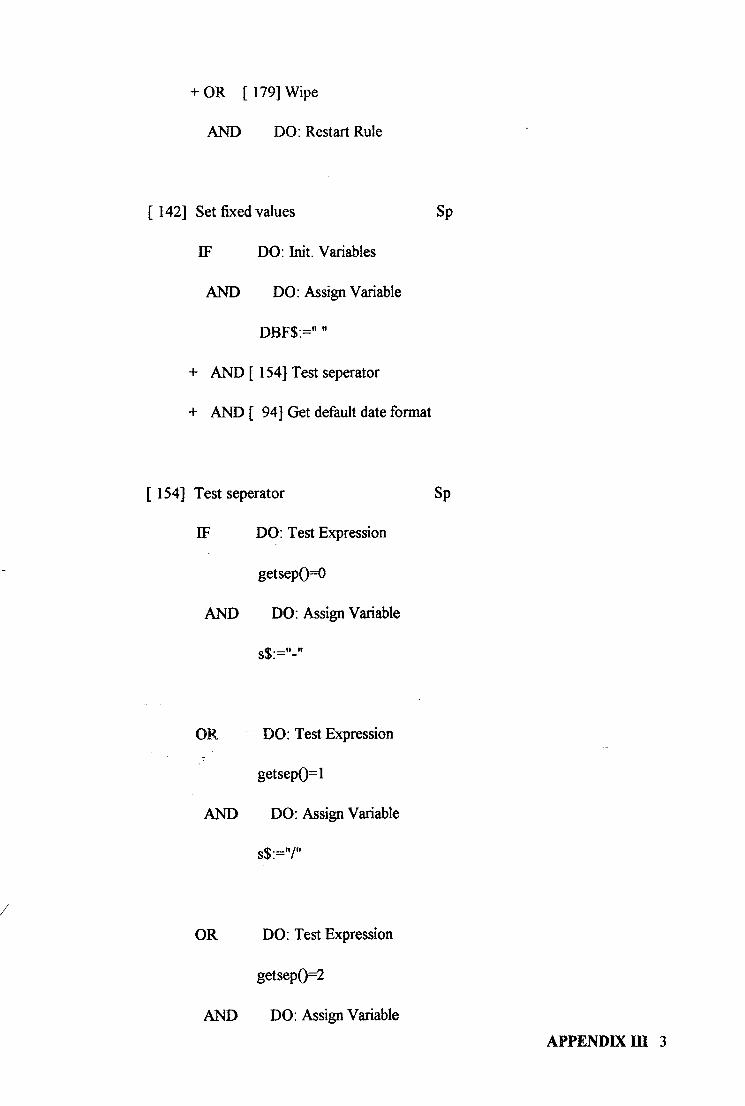
+ 0 R [179] Wipe
AND DO: Restart Rule
[ 142] Set fixed values Sp
IF DO: Init. Variables
AND DO: Assign Variable
DBF$:=""
+ AND [ 154] Test seperator
+ AND[ 94] Get default date format
[ 154] Test seperator Sp
IF DO: Test Expression
getsepO=0
AND DO: Assign Variable
$$:="-"
OR DO: Test Expression
getsepO=l
AND DO: Assign Variable
s$:=7"
OR DO: Test Expression
getsep0=2
AND DO: Assign Variable
APPENDIX m 3

s$:="."
[ 94] Get default date format Sp
IF DO: Test Expression
getformO=0
AND DO: Assign Variable
df$:-"DD"+s$+"MM"+s$+"YYYY"
OR DO: Test Expression
getformO=l
AND DO: Assign Variable
df$:="MM"+s$+"DD''+s$+"YYYY"
OR DO: Test Expression
getform0=2
AND DO: Assign Variable
df$:="YYYY"+s$+"MM"+s$+"DD''
[31] Check interface is loaded Sp
+ IF [ 38] Clear error flag
AND DO: Test Expression
verify("dbcr")
+ AND[ 27] Check for error
APPENDDCm 4

F OR DO: Display Form
AND DO: Quit
[ 38] Clear error flag Sp
IF DO: Test Expression
errclrO
[ 27] Check for error Sp
IF DO: Test Expression
errokO
Closedown Sp
+ IF [ 38] Clear error flag
AND DO: Test Expression
DBcloseallO
+ AND[ 27] Check for error
[ 124] Open file Sp
IF DO: Assign Variable
drfli:=DBopen("a:\dsss")
AND DO: Assign Variable
drflil:=DBopen("a:\INV")
AND DO: Assign Variable
drfli2:=DBopen("a:\req")
APPENDIX m 5

[ 138] Select database fflel Sp
+ IF [ 38] Clear error flag
AND DO: Test Expression
DBselect(drfli)
+ AND[ 27] Check for error
AND DO: Assign Variable
INAMEF:=DBiopen("a:\IDSSs.CRX")
AND DO: Test Expression
DBorder(INAMEF)
[103] Goto first Sp
+ IF [ 38] Clear error flag
AND DO: Test Expression
DBfirstO
+ AND[ 27] Check for error
AND DO: Assign Variable
theo:=0
[ 39] Clear out fields Sp
IF DO: Test Expression
arrclr(dt$[#])
AND DO: Test Expression
arrclr(dt[#])
APPENDIX in 6

[130] Read data Sp
+ IF [ 115] Load all fields
+ AND [ 150] Test for delete mark
AND DO: Assign Variable
recsub:=0
+ AND[ 54] Convert to text
AND DO: FaU
OR DO: Succeed
[115] Load aU fields SpEx
IF DO: Test Expression
erronO
AND DO: Test Expression
DBreadrec(dt[#])
AND DO: Test Expression
DBreadrec(dt$[#])
AND DO: Assign Variable
recsub:=0
[ 150] Test for delete mark
+ IF [162] Turn off errors
+ AND[ 62] Delete record
AND DO: Assign Variable
Sp • /
APPENDIX III 7

recdel:=0
+ AND [ 133] Recall record
OR DO: Assign Variable
recdel:=l
[ 162] Turn off errors Sp
IF DO: Test Expression
errofifO
[ 62] Delete record Sp
+ IF [ 38] Clear error flag
AND DO: Test Expression
DBdelete(DBrecnoO)
+ AND [ 27] Check for error
[ 133] Recall record Sp
+ IF [ 38] Clear error flag
AND DO: Test Expression
DBrecaIl(DBrecnoO)
+ AND[ 27] Check for error
/
[ 54] Convert to text Sp
IF DO: Assign Variable
cnt:=0 APPENDIX m 8

+ AND[ 47] Convert loop
[ 47] Convert loop Sp
IF DO: Test Expression
b$[cnt]="N"
AND DO: Assign Variable
dt$[cnt]:=string$(dt[cnt],c[cnt],d[cnt])
AND DO: Fail
OR DO: Test Expression
b$[cnt]="L"
AND DO: Assign Variable
dt$[cnt]:=query$(dt[cnt],"T","F")
AND DO: Assign Variable
dt[cnt]:=0
AND DO: Fail
/
OR DO: Test Expression
b$[cnt]="D"
AND DO: Assign Variable
dt$[cnt]:=date$(dt[cnt])
AND DO: Assign Variable
dt[cnt]:=0
AND DO: Fail
APPENDKm 9

OR DO: Assign Variable
cnt:=cnt+l
AND DO: Test Expression
cnt<nof
AND DO: Restart Rule
OR DO: Succeed
[ 179] Wipe Sp
+ IF DO: Wipe Rule
Set fixed values
AND DO: Wipe Rule
Ask for filename
[ 67] display the requirements Sp
+ IF [103] Goto first
+ AND[ 78] find the day's orders
[ 78] find the day's orders Sp
IF DO: Assign Variable
today:=nowO
AND DO: Assign Variable
i:=0
+ AND[ 83] find the record
AND DO: Test Expression
ioO
[ 83] find the record Sp
APPENDIX m 10

+ IF [ 130] Read data
AND DO: Assign Variable
recdatef$:=dt$[2]
AND DO: Assign Variable
recdatef=date(recdatef$)
+ AND [ 158] test today
AND DO: Restart Rule
OR DO: Succeed
[ 158] test today Sp
IF DO: Assign Variable
today$:=date$(today)
AND DO: Assign Variable
recdatefS :=date$(recdateO
AND DO: Test Expression
today$=recdatef$
AND DO: Assign Variable
ordnb$[i]:=dt$[l]
AND DO: Assign Variable
i:=i+l
+ AND [ 105] Goto next
+ OR [ 105] Goto next
APPENDIX ffl 11

[ 105] Goto next Sp
+ IF [ 38] Clear error flag
AND DO: Test Expression
DBnextO
+ AND[ 27] Check for error
[ 145] START UPDATING THE INV REQ AND DSS Sp
+ IF [121] Maintain a general database
[ 121] Maintain a general database SpEx
+ IF [ 112] Initialise
+ AND [ 166] Update database
+ AND [ 135] req
+ AND [ 44] Closedown
AND DO: Restart Rule
[ 166] Update database Sp
+ IF [ 3 ] Action menu
+ AND[ 69] Do action
AND DO: Test Expression
! finished
+ AND[ 130] Read data
AND DO: Restart Rule
+ 0 R [179] Wipe
APPENDIX i n 12

[ 69] Do action Sp
IF DO: Assign Variable
sact$:=left$(act$,l)
AND DO: Test Expression
!("U"=sact$)
+ AND[ 39] Clear out fields
AND DO: FaU
OR DO: Test Expression
"N"=sact$
+ AND [ 105] Goto next
OR DO: Test Expression
"P"=sact$
AND DO: Test Expression
act$="Prior"
+ AND [ 106] Goto prior
OR DO: Test Expression
"F"=sact$
+ AND [ 103] Goto first
OR DO: Test Expression
"L"=sact$ APPENDIX ra 13

+ AND[ 104] Goto last
OR DO: Test Expression
"A"=sact$
+ AND[ 4] Add record
OR DO: Test Expression
"U"=sact$
+ AND [ 167] Update menu
OR DO: Test Expression
"Q"=sact$
AND DO: Assign Variable
finished:=l
OR DO: Test Expression
"D"=sact$
AND DO: Test Expression
(recdel
+ AND [ 162] Turn off errors
+ AND[ 62] Delete record
OR DO: Test Expression
"R"=sact$
APPENDIX i n 14

AND DO: Test Expression
recdel
+ AND [ 162] Turn off errors
+ AND [133] Recall record
OR DO: Test Expression
act$="Pack"
+ AND [ 127] Pack
OR DO: Succeed
[ 106] Goto prior Sp
+ IF [ 38] Clear error flag
AND DO: Test Expression
DBpriorO
+ AND ( 27] Check for error
[ 104] Goto last Sp
+ IF [ 38] Clear error flag
AND DO: Test Expression
DBlastO
+ AND [ 27] Check for error
[ 4] Add record Sp
IF DO: Assign Variable
APPENDIX DI 15

drinkno:=DBappendO
+ AND [ 91] Get data
+ AND [ 180] Write data record
[ 91] Get data Sp
F IF DO: Help Explain
AND DO: Fail
+ AND [ 176] update the supporting files
+ OR [ 52] Convert to numbers
[ 176] update the supporting files Sp
+ IF [171] update the db when update and delete
[171] update the db when update and delete Sp
+ IF [72] estimate requirements for up and del
+ AND [137] select database
+ AND [ 103] Goto first
AND DO: Assign Variable
nofl:=DBgetflds(invl$[#],invl l$[#],invl[#],invl 1[#])
+ AND[ 40] clear out fields for invl
+ AND [ 132] read data form invl file
+ AND [ 25] check date with in the week for mvl for up&del • /
+ 0 R [ 179] Wipe
[ 72] estimate requirements for up and del Sp
APPENDIX n i 16

IF DO: Assign Variable
deli:=date(oldval$[2]) AND DO: Assign Variable
daynam$:=left$(day$(deli),3)
[137] select database Sp
+ IF [139] select db
[ 139] select db Sp
+ IF [ 38] Clear error flag
AND DO: Test Expression
DBselect(drfhl)
+ A N D [ 27] Check for error
[ 40] clear out fields for invl Sp
IF DO: Test Expression
arrclr(dtinvl$[#])
AND DO: Test Expression
arrclr(dtinvl[#])
[ 132] read data form invl file Sp
+ IF [ 117] load all fldsinvl
+ AND [ 151 ] test for delete mark for inv 1
AND DO: Assign Variable
recsubil:=0
+ AND [ 55] convert to text for invl
[ 117] load aU fldsinvl Sp
APPENDIX in 17

IF DO: Test Expression
erronQ
AND DO. Test Expression
DBreadrec(dtinvl[#])
AND DO: Test Expression
DBreadrec(dtinv !$[#])
AND DO: Assign Variable
recsubil:=0
[151] test for delete mark for invl Sp
+ IF [162] Turn off errors
+ A N D [ 62] Delete record
AND DO: Assign Variable
recdelil:=0
+ AND [ 133] Recall record
OR DO: Assign Variable
ref^elil:=l
[ 55] convert to text for invl Sp
IF DO: Assign Variable
cntil:=0
+ AND [ 50] convert loop for invl
[ 5 0 ] convert loop for invl Sp
IF DO: Test Expression
invll$[cntil]="N"
APPENDIX ffl 18

AND DO: Assign Variable
dtinv 1 $[cnti 1 ] :=string$(dtinvl [cnti 1 ],inv 1 [cnti 1 ],inv 11 [cnti 1 ])
AND DO: Fail
OR DO: Test Expression
invll$[cntil]="L"
AND DO: Assign Variable
dtinv 1 $[cntil ]:-query$(dtinv 1 [cnti 1 ] , "T","F")
AND DO: Assign Variable
dtinvl[cntil]:=0
AND DO: Fail
OR DO: Test Expression
invll$[cntil]="D"
AND DO: Assign Variable
dtinvl $[cnti 1] :=date$(dtinvl [cntil ])
AND DO: Assign Variable
dtinvl [cntil]:=0
AND DO: Fail
OR DO: Assign Variable
cntil :==cntil+l
AND DO: Test Expression
cntil<nofl
APPENDIX m 19

AND DO: Restart Rule
OR DO; Succeed
[ 25] check date with in the week for invl for up&del Sp
+ IF [ 93] get date for invl
AND DO: Assign Variable
daynam$:=left$(day${deli),3)
+ A N D [ 77] find the day for up and del
[ 93] get date for invl Sp
+ IF [ 11] assign the dates
AND DO: Test Expression
i foundi to i
AND DO: Restart Rule
OR DO: Succeed
[ 11] assign the dates Sp
+ IF [132] read data form invl file
AND DO: Assign Variable
delinvl$:=dtinvl$[0]
AND DO: Assign Variable
delinvl :=int(date(delinvl $))
AND DO: Assign Variable
deleinl$:=dtinvl$[l]
APPENDIX in 20

AND DO: Assign Variable
deleinl :=int(date(deleinl$))
W AND DO: Display Form
AND DO: Test Expression
deli>=delinvl
AND DO: Test Expression
deli<=deleinl
AND DO: Assign Variable
ifoundit:=l
+ 0R [ 105] Goto next
AND DO: Assign Variable
ifoundit:=0
[ 77] find the day for up and del Sp
IF DO: Assign Variable
cnti:=2
+ AND [ 90] get and check the day fi-om invl for up and del
[ 90] get and check the day fi-om invl for up and del Sp
+ IF [132] read data form invl file
AND DO: Assign Variable /
daynaml $:=left$(invl $[cnti],3)
+ A N D [ 28] check for up and del
APPENDIX m 21

W OR DO: Display Form
[ 28] check for up and del Sp
+ IF [132] read data form invl file
AND DO: Test Expression
(daynam 1 $odaynam$)
AND DO: Assign Variable
cnti:=cnti+2
AND DO: Test Expression
cnti<=10
AND DO: Assign Variable
daynaml $:=left$(invl $[cnti],3)
AND DO: Restart Rule
WOR DO: Display Form
+ AND [ 24] check balance for up and del
[ 24] check balance for up and del Sp
W I F DO: Display Form
AND DO: Test Expression
dtinvl [cnti+1 ]>value(dtinvl $[cnti+l ])
AND DO: Assign Variable
dtinv 1 [cnti+1 ] :=value(dtinvl $[cnti+1 ])-value(oldval$[4]) • /
AND DO: Assign Variable
dtinvl[cnti]:=value(dtinvl$[cnti])-value(oldval$[cnti])
AND DO: Assign Variable
APPENDIX ffl 22

dtinvl [0] :=date{dtinvl $[0])
AND DO: Assign Variable
dtinvl [l]:=date(dtinvl$[l])
AND DO: Test Expression
DBwriterec(dtinvl [#])
AND DO: Test Expression
DBwriterec(dtinv 1 $[#])
AND DO; Test Expression
DBselect(drfli)
W OR DO: Display Form
WPOS: 2,15,10,50
[ 52] Convert to numbers Sp
+ IF [128] Prepare for convert
+ A N D [ 48] Convert loop back
[ 128] Prepare for convert Sp
IF DO: Assign Variable
hsh$~"mmmmmmmm#"
AND DO: Assign Variable
cnt:=0
+ A N D [ 37] Clear dt[#] • /
[ 37] Clear dt[#] Sp
IF DO: Test Expression
APPENDIX in 23

arrclr(dt[#])
[ 48] Convert loop back Sp
IF DO: Test Expression
b$[cnt]="N"
+ AND [ 122] Number conversion back
AND DO: FaU
OR DO: Test Expression
b$[cnt]="L"
+ AND [119] Logical convertion back
AND DO: Fail
OR DO: Test Expression
b$[cnt]="D"
+ AND [ 162] Turn off errors
+ A N D [ 38] Clear error flag
+ AND [ 147] Tate conversion back
A l ^ DO: Fail
OR DO: Assign Variable
cnt:=cnt+l
AND DO: Test Expression
cnt<nof
AND DO: Restart Rule
/
APPENDIX ffl 24

OR DO: Succeed
[ 122] Number conversion back Sp
IF DO: Assign Variable
dt[cnt]:=value(dt$[cnt])
AND DO: Assign Variable
ll:=c[cnt]-d[cnt]-(d[cnt]>0)
AND DO: Test Expression
dt[cnt]<10'^U
OR DO: Assign Variable
form$:=left$(hsh$,ll)+"."+left$(hsh$,d[cnt])
AND DO: Assign Variable
prob$:="Invalid Number Use format "H-formS
+ A N D [ 89] Fix errors
[ 89] Fix errors Sp
F IF DO: Help Explain
AND DO: Assign Variable
cnt:=cnt-l
[119] Logical convertion back Sp
IF DO: Assign Variable
e$:=dt$[cnt]
AND DO: Test Expression
APPENDIX m 25

e$-"T"|e$=" 1 "|e$="true"|e$="Y"|e$="Yes"
AND DO: Assign Variable
dt$[cnt]:="T"
AND DO: Assign Variable
dt[cnt]:=l
OR DO: Assign Variable
dt$[cnt]:="F"
AND DO: Assign Variable
dt[cnt]:=0
[147] Tate conversion back Sp
IF DO: Assign Variable
dt[cnt]:=date(dt$[cnt])
+ AND [ 27] Check for error
OR DO: Assign Variable
prob$:=''Invalid Date Please Reenter as ''+dt$
+ A N D [ 89] Fix errors
[ 180] Write data record Sp
IF DO: Test Expression
DBwriterec(dt$[#])
AND DO: Test Expression
APPENDIX m 26

DBwriterec(dt[#])
[ 167] Update menu Sp + IF [ 9 1 ] Get data + AND [ 180] Write data record
[ 127] Pack Sp
+ IF [ 38] Clear error flag
AND DO: Test Expression
DBpackO
+ A N D [ 27] Check for error
[ 135] req Sp
+ IF [ 103] Goto first
AND DO: Assign Variable
last:=0
AND DO: Assign Variable
lastsos:=0
+ A N D [ 7] arrest
[ 7] arrest Sp
+ IF [100] getdate
+ AND [ 22] check and estimate
AND DO: Test Expression
lastsos^O
AND DO: Restart Rule
[ 100] getdate Sp
APPENDIX m 27

+ IF [ 130] Read data
AND DO: Assign Variable
deli$:=dt$[2]
AND DO: Assign Variable
deli:=date(deli$)
AND DO: Assign Variable
theol:=0
AND DO: Assign Variable
ind:=l
[ 22] check and estimate Sp
+ IF [ 29] check i f it is estimated
OR DO: Test Expression
last=l
[ 29] check i f i t is estimated Sp
+ IF [ 153] test i f yes
+ AND [181] write the new data
+ AND [ 45] continue the calcu
+ 0R [ 30] check i f this is the last
AND DO: Assign Variable
last:-l
+ AND [ 130] Read data
/
APPENDIX m 28

AND DO: Assign Variable
deli$:=<it$[2]
AND DO: Test Expression
deli=date(deli$)
[ 153] test i f yes Sp
IF DO: Test Expression
dt$[0]="F"
AND DO: Assign Variable
theol:=theol+dt[4]
[ 181] write the new data Sp
IF DO: Assign Variable
dt$[0]:="T"
AND DO: Assign Variable
dt[0]:=l
AND DO: Assign Variable
dt[l]:-value(dt$[l])
AND DO: Assign Variable
dt[2]:=date(dt$[2])
AND DO: Assign Variable
dt[3]:=date(dt$[3])
AND DO: Assign Variable
dt[5]:=value(dt$[5])
AND DO: Test Expression
/
APPENDIX in 29

DBwriterec(dt$[#])
AND DO: Test Expression
DBwriterec(dt[#])
[ 45] continue the calcu Sp
+ IF [ 178] where to go
+ AND [ 130] Read data
AND DO: Assign Variable
delic$:=dt$[2]
AND DO; Test Expression
deli=int(date(delic$))
AND DO: Restart Rule
+ 0R [ 68] distribute
[ 178] where to go Sp
+ IF [ 2 1 ] CHECK AGAIN IF IT IS BEEN CHECKED
OR DO; Fail
[ 21] CHECK AGAIN IF IT IS BEEN CHECKED Sp
+ IF [105] Goto next
+ AND [ 130] Read data
AND DO: Assign Variable
sos:=l
AND DO: Assign Variable
deU$:=dt$[2]
APPENDIX ffl 30

/
AND DO: Test Expression
deli-date(deli$)
AND DO: Assign Variable
sos:=0
AND DO: Test Expression
dt$[0]=T
AND DO: Assign Variable
dt$[0]:="T"
AND DO: Assign Variable
dt[0]:=l
AND DO: Assign Variable
dt[l]:-value(dt$[l])
AND DO: Assign Variable
dt[2]:=date(dt$[2])
AND DO: Assign Variable
dt[3]:=date(dt$[3])
AND DO: Assign Variable
dt[5]:=value(dt$[5])
AND DO; Test Expression
DBwriterec(dt[#])
AND DO; Test Expression
DBwriterec(dt$[#])
AND DO: Assign Variable
theol:=theol+dt[4]
APPENDIX in 31

/
OR DO: Test Expression
sos=0
+ AND [ 105] Goto next
OR DO: Fail
[ 68] distribute Sp
+ IF [ 75] find date
+ AND [137] select database
+ AND [ 103] Goto first
AND DO; Assign Variable
nofl :=DBgetflds(invl$[#],invl l$[#],invl[#],invl 1[#])
+ AND [ 40] clear out fields for invl
+ AND [ 132] read data form invl file
+ AND [ 107] heck date vwth in the week for invl
+ OR [179] Wipe
[ 75] find date Sp
IF DO: Assign Variable
daynam$:=day$(deli)
[ 107] heck date with in the week for invl Sp
APPENDIX ffl 32

+ IF [ 93] get date for invl
AND DO: Assign Variable
daynam$:=left$(day$(deli),3)
+ AND [ 110] ind the day
[110] ind the day Sp
IF DO: Assign Variable
cnti:=2
+ AND [ 99] getand check the day from invl
[ 99] getand check the day from invl Sp
+ IF [132] read data form invl file
AND DO: Assign Variable
daynaml $:=left$(invl $[cnti],3)
+ AND [ 20] check
W OR DO: Display Form
WPOS: 2,15,10,50
AND DO: Fail
[ 20] check Sp
+ IF [132] read data form invl file
APPENDIX in 33

AND DO: Test Expression
(daynam 1 $odaynani$)
AND DO: Assign Variable
cnti:=cnti+2
AND DO: Test Expression
cnti<=10
AND DO: Assign Variable
daynam 1 $: =left$(inv 1 $[cnti], 3)
AND DO: Restart Rule
+ 0R [ 23] check balance
[ 23] check balance Sp
IF DO: Test Expression
dtinv 1 [cnti]-dtinv 1 [cnti+1 ]>=theo 1
+ AND [ 165] update and allocate
+ OR [ 134] release a kanban order
[ 165] update and allocate Sp
IF DO: Assign Variable
dtinvl [cnti+1 ]:=value(dtinvl $[cnti+1 ])+theo 1
AND DO: Assign Variable
dtinvl [0]:=date(dtinvl$[0])
APPENDIX i n 34

AND DO: Assign Variable
dtinvl[l]:=date(dtinvl$[l])
AND DO: Test Expression
DBwriterec(dtinv 1 [#])
AND DO: Test Expression
DBwriterec(dtinvl $[#])
+ AND [ 173] update the foUowing's day inv
AND DO: Test Expression
DBselect(drfli)
W OR DO: Display Form
WPOS: 2,15,10,50
Could you please add more.inventory records
because I can not schedule the orders
AND DO: Fail
[173] update the follovwng's day inv Sp
+ IF [132] read data form invl file
AND DO: Assign Variable
difiFer;=value(dtinvl$[cnti])-value(dtinvl$[cnti+l])
+ AND [ 160] the next record inv
+ A N D [ 70] do it for all the inv records
AND DO: Restart Rule
APPENDIX ffl 35

OR DO: Succeed
[160] the next record inv Sp
IF DO: Test Expression
cnti<=8
AND DO: Test Expression
difFer>=value(dtinvl $[cnti+3 ])
AND DO: Assign Variable
dtinv l[cnti+2]:=differ
AND DO: Assign Variable
dtinvl [0] :=date(dtinvl $[0])
AND DO: Assign Variable
dtinvl [l]:=date(dtinvl$[l])
AND DO: Test Expression
DBwriterec{dtinv 1 [#])
AND DO: Test Expression
DBwriterec{dtinvl$[#])
+ A N D [ 2] ***AVE TO FIND THE DATE AND CHANGECNTI
+ A N D [ 16] cancel the release of kanban orders
OR DO: Test Expression
cnti<=8
+ AND [ 136] rescheduling
OR DO: Succeed
APPENDIX m 36

[ 2] ***AVE TO FIND THE DATE AND CHANGECNTI Sp
IF DO: Assign Variable
STARTD:=date(dtinvl$[0])
AND DO: Assign Variable
datenaml $:=left$(invl $[cnti+2],3)
[ 16] cancel the release of kanban orders Sp
+ IF [ 111] init the requiremetns
+ AND [ 26] CHECK DATES FOR REQUIREMENTS
AND DO: Assign Variable
cntr:=2
+ A N D [ 64] delete the orders
+ AND [131] read data for requirements
AND DO: Test Expression
DBselect(drflil)
+ AND [ 132] read data form invl file
[111] init the requiremetns Sp
+ IF [140] select requirements
+ AND [ 103] Goto first
, AND DO: Assign Variable
no£2:=DBgetflds(reql$[#],reql l$[#],reql[#],reql 1[#]) ' /
+ AND [ 4 1 ] clear out fileds for requirements
+ AND [131] read data for requirements
[ 140] select requirements Sp APPENDIX m 37

+ IF [ 38] Clear error flag
AND DO: Test Expression
DBselect(drfh2)
+ A N D [ 27] Check for error
[ 4 1 ] clear out fileds for requirements Sp
IF DO: Test Expression
arrch-(dtreq$[#])
AND DO: Test Expression
arrclr(dtreq[#])
[131] read data for requirements Sp
+ IF [116] load all fields for requirements
+ AND [ 152] test for delete mark for requirements
+ AND [ 56] convert to text for requirements
[116] load all fields for requirements Sp
IF DO: Test Expression
erronO
AND DO: Test Expression
DBreadrec(dtreq$[#])
AND DO: Test Expression
DBreadrec(dtreq[#])
AND DO: Assign Variable
APPENDIX m 38

recsuc2:=0
[ 152] test for delete mark for requirements Sp
+ IF [ 162] Turn off errors
+ A N D [ 62] Delete record
AND DO: Assign Variable
recdel2:=0
+ AND [ 133] Recall record
OR DO: Assign Variable
recdel2:=l
[ 56] convert to text for requirements Sp
IF DO: Assign Variable
cntr:=0
+ AND [ 5 1 ] convert loop for requirements
[ 51] convert loop for requirements Sp
IF DO: Test Expression
reqll$[cntr]="N"
AND DO: Assign Variable
dtreq$[cntr] :=string$(dtreq[cntr],req 1 [cntr],req 11 [cntr])
AND DO: Fail
APPENDIX i n 39

OR DO: Test Expression
reqll$[cntr]="L"
AND DO: Assign Variable
dtreq$[cntr]:-query$(dtreq[cntr],"T","F")
AND DO: Assign Variable
dtreq[cntr]:=0
AND DO: Fail
OR DO: Test Expression
reqll$[cntr]="D"
AND DO: Assign Variable
dtreq$[cntr] :=date$(dtreq[cntr])
AND DO: Assign Variable
dtreq[cntr]:=0
AND DO.FaH
OR DO: Assign Variable
cntr:=cntr+l
AND DO: Test Expression
cntr<nof2
AND DO: Restart Rule
OR DO: Succeed
APPENDIX m 40

[ 26] CHECK DATES FOR REQUIREMENTS Sp
+ IF [ 8 4 ] find the record for the requirements
AND DO: Test Expression
r foundi to l
AND DO: Restart Rule
OR DO: Succeed
[ 84] find the record for the requirements Sp
+ IF [131] read data for requirements
AND DO: Assign Variable
DELIREQ:=int(date(dtreq$[0]))
AND DO: Assign Variable
DELEREQ:=int(date(dtreq$[l]))
AND DO: Test Expression
deU-7<=DELEREQ
AND DO: Test Expression
deli-7>=DELIREQ
AND DO: Assign Variable
rfoundit:=l
+ OR [ 105] Goto next
AND DO: Assign Variable
rfoundit:=0
/
APPENDIX ffl 41

[ 64] delete the orders Sp
IF DO: Assign Variable
DAYNMRS :=left$(req 1 $[cntr],3)
AND DO: Test Expression
datenam I $ o D A YNMR$
AND DO: Assign Variable
cntr:==cntr+l
AND DO: Restart Rule
+ OR [ 1 7 ] cancel the scheduled orders
[ 17] cancel the scheduled orders ' Sp
IF DO: Assign Variable
dtreq[0] :=date(dtreq$[0])
AND DO: Assign Variable
dtreq[ 1 ] :=date(dtreq$[ 1 ])
AND DO: Assign Variable
dtreq[cntr]:=0
AND DO: Test Expression
DBwriterec(dtreq[#]) /
AND DO: Test Expression
DBwriterec(dtreq$[#])
+ AND [131] read data for requirements APPENDIX m 42

AND DO: Test Expression
DBselect(drflil)
[136] rescheduHng Sp
IF DO: Assign Variable
demand:=value(dtinv 1 $[cnti+3])-diflfer
AND DO: Assign Variable
quantity:=demand
+ AND [ 156] test the remainder to update the inv for resc
+ AND [ 182] write the new data in inv
+ A N D [ 2] ***AVE TO FIND THE DATE AND CHANGECNTI
+ AND [ 169] update requirements in rescheduling
AND DO: Test Expression
DBselect(drflil)
+ AND [ 132] read data form invl file
[ 156] test the remainder to update the inv for resc Sp
IF DO: Test Expression
quantity/10>=1
+ AND [ 109] i f it is indeed
/ OR DO: Assign Variable
dtinvl [cnti+2]:=10+dififer
AND DO: Assign Variable
APPENDIX m 43

nbrord:=l
[ 109] i f i t is indeed Sp
IF DO: Test Expression
mod(quantity, 10)=0
AND DO: Assign Variable
dtinvl [cnti+2] :=value(dtinv 1 $[cnti+2])+quantity
AND DO: Assign Variable
nbrord:=quantity/10
OR DO: Assign Variable
dtinv 1 [cnti+2]: =value(dtinv 1 $[cnti+2]>f quantity+10-
mod(quantity,10)
AND DO: Assign Variable
nbrord:=int(quantity/10)+1
[ 182] write the new data in inv Sp
IF DO: Assign Variable
dtinv 1 [0] :=date(dtinvl $[0])
AND DO: Assign Variable
dt inv 1 [ 1 ] : =dat e(dtinv 1 $ [ 1 ])
/ AND DO: Test Expression
DBwriterec(dtinvl [#])
AND DO: Test Expression
APPENDIX m 44

/
DBwriterec(dtinvl$[#])
[169] update requirements in rescheduling Sp
IF DO: Test Expression
DBselect(drfh2)
+ AND [ 111] init the requiremetns
+ AND [ 26] CHECK DATES FOR REQUIREMENTS
AND DO: Assign Variable
cntr:=2
+ AND [ 59] day for requirements rescheduling
[ 59] day for requirements rescheduling Sp
+ IF [ 1 0 ] assign cntr value
+ AND [ 126] overwrite the requirements
[ 10] assign cntr value Sp
IF DO: Test Expression
cnti+2=2
AND DO: Assign Variable
cntr:=2
OR DO: Test Expression
cnti+2=4
AND DO: Assign Variable
APPENDIX in 45

cntr:=3
OR DO: Test Expression
cnti+2=6
AND DO: Assign Variable
cntr:=4
OR DO: Test Expression
cnti+2=8
AND DO: Assign Variable
cntr:=5
OR DO: Test Expression
cnti+2=10
AND DO: Assign Variable
cntr:=6
[126] overwrite the requirements Sp
IF DO: Assign Variable
dtreq[cntr]:=nbrord
AND DO: Assign Variable
dtreq[0]:=date(dtreq$[0])
AND DO: Assign Variable
dtreq[l]:=date(dtreq$[l])
APPENDIX ffl 46

AND DO: Test Expression
DBwriterec(dtreq[#])
AND DO: Test Expression
DBwriterec(dtreq$[#])
AND DO: Test Expression
DBselect(drflil)
[ 70] do it for all the inv records Sp
IF DO: Assign Variable
cnti:=cnti+2
AND DO: Test Expression
cnti<=10
OR DO: Assign Variable
differ:=value(dtinvl $[cnti-2])-value(dtinvl $[cnti-1 ])
+ AND [ 105] Goto next
+ AND [ 132] read data form invl file
AND DO: Assign Variable
deli:=deli+7
AND DO: Assign Variable
cnti:=0
+ AND [ 160] the next record inv
AND DO: Assign Variable
cnti:=cnti+2
APPENDIX n i 47

[134] release a kanban order Sp
+ IF [ 33] check the lead time
AND DO: Assign Variable
quantity:=theol-(value(dtinvl $[cnti])-va]ue(dtinvl $[cnti+l]))
AND DO: Assign Variable
dtinvl [cnti+1 ] :-value(dtinv 1 $[cnti+1 ])+theo 1
+ AND [155] test the remainder to update the inv
AND DO: Assign Variable
dtinvl [0] :=date(dtinvl $[0])
AND DO: Assign Variable
dtinvl [ 1 ] :=date(dtinvl $[ 1 ])
AND DO: Test Expression
DBwriterec(dtinvl[#])
AND DO: Test Expression
DB writerec(dtinv 1 $[#])
+ AND [ 175] update the requirements
+ AND [ 173] update the following's day inv
AND DO: Test Expression
DBselect(drfh)
W OR DO: Display Form
WPOS: 2,15,10,50
APPENDIX ffl 48

You have to delay the order because there is
not enough time for production
COL : SURR Yellow on Red
COL: 0,0 YeUowonRed
+ AND [ 19] change the log at the assembly file
AND DO: Quit
[33] check the lead time Sp
IF DO: Assign Variable
clead:=nowO
AND DO: Test Expression
clead<=deli+7
OR [161] their is no time for the fabn
AND DO: Fail
[161] their is no time for the fabn Sp
[155] test the remainder to update the inv Sp
IF DO: Test Expression
quantity/10>=1
+ AND [ 108] if it is /
OR DO: Assign Variable
APPENDIX m 49

dtinv 1 [cnti] :=value(dtinv 1 $[cnti])+10
AND DO: Assign Variable
nbrord:=l
[ 108] if it is Sp
IF DO: Test Expression
mod(quantity,10)=0
AND DO: Assign Variable
dtinv 1 [cnti] :=value(dtinv 1 $[cnti])+quantity
AND DO: Assign Variable
nbrord:=quantity/10
OR DO: Assign Variable
dtinvl [cnti] :=value(dtinvl $[cnti])+qxmntity+10-mod(quantity, 10)
AND DO: Assign Variable
nbrord:=int(quantity/10)+1
[ 175] update the requirements Sp
+ IF [ 111 ] init the requiremetns
+ AND [ 26] CHECK DATES FOR REQUIREMENTS
AND DO: Assign Variable • / '
cntr:=2
+ AND [ 96] GET THE DAY FOR REQUIREMENTS
+ AND [131] read data for requirements APPENDIX m 50

AND DO: Test Expression
DBselect(drfhl)
[ 96] GET THE DAY FOR REQUIREMENTS Sp
IF DO: Assign Variable
DAYNMR$:=left$(reqI $[cntr],3)
AND DO: Test Expression
daynaml $oDAYNMR$
AND DO: Assign Variable
cntr:=cntr+l
AND DO: Test Expression
cntr<7
AND DO: Restart Rule
+ OR [172] UPDATE THE DBFILE WITH THE NEW REQUIREMENTS
[ 172] UPDATE THE DBFILE WITH THE NEW REQUIREMENTS Sp
IF DO: Assign Variable
dtreq[cntr] :=value(dtreq$[cntr])+nbrord
AND DO: Assign Variable
/ dtreq[0]:=date(dtreq$[0])
AND DO: Assign Variable
dtreq[ 1 ] :=date(dtreq$[ 1 ])
APPENDIX ffl 51

AND DO: Test Expression
DBwriterec(dtreq[#]) AND DO: Test Expression
DBwriterec(dtreq$[#])
[ 19] change the log at the assembly file Sp
IF DO: Test Expression
DBselect(drfh)
AND DO: Assign Variable
dt[0]:=O
AND DO: Assign Variable
dt[l]:=value(dt$[l])
AND DO: Assign Variable
dt[2]:=date(dt$[2])
AND DO: Assign Variable
dt[3];=date(dt$[3])
AND DO: Assign Variable
dt[5]:-value(dt$[5])
AND DO: Test Expression
DBwriterec(dt[#])
AND DO: Test Expression
DBwriterec(dt$[#])
[ 30] check if this is the last Sp
APPENDIX in 52

+ IF [ 105] Goto next
OR DO: Assign Variable
lastsos:=l
[ 43] CLOSE THE ORDERS IN DSS Sp
+ IF [ 112] Initialise
W AND DO: Display Form
WPOS: 1,1,23,78
could you pis type in the nimiber of the orders that are finished?
+ AND [ 103] Goto first
AND DO: Assign Variable
i:=0
+ AND[ 81]findthejobsl
[ 81 ] find the jobsl Sp
+ IF [ 80] find the jobs
AND DO: Restart Rule
[ 80] find thejobs Sp
APPENDIX ni 53

+ IF [ 130] Read data
AND DO: Test Expression
order$[i]=dt$[l]
AND DO: Assign Variable
i:=i+l
+ AND [ 42] close the ord
+ AND [ 105] Goto next
+ OR [ 105] Goto next
[ 42] close the ord Sp
IF DO: Assign Variable
dt[5]:=l
AND DO: Assign Variable
dt[2]:=date(dt$[2])
AND DO: Assign Variable
dt[3]:=int(nowO)
AND DO: Assign Variable
dt[0]:=value(dt$[0])
AND DO: Assign Variable
dt[4]:=value(dt$[4])
AND DO: Assign Variable
dt[l]:=value{dt$[l])
AND DO: Test Expression APPENDIX m 54

DBwriterec(dt[#])
AND DO: Test Expression
DBwriterec(dt$[#])
[ 125] OPEN REQ AND GET DATA Sp
+ IF [142] Set fixed values
+ AND[ 44] Closedown
AND DO: Assign Variable
drfli2:=DBopen("a:\req")
+ AND [ 111] init the requiremetns
+ AND [ 103] Goto first
+ AND[ 88] find today's requirements
+ AND [ 44] Closedown
[ 88] find today's requirements Sp
IF DO: Assign Variable
today:=nowO
+ AND[ 85] find the record in the rq
W AND DO: Display Form
WPOS: 1,1,23,78
The number of orders that should be released today is: / •
* [nbrreq$ ] *
APPENDIX ffl 55

You have to receive today [nbre] of kanban containers
W OR DO: Display Form
WPOS: 2,15,10,50
There are no orders to be released.
[ 85] find the record in the rq Sp
+ IF [131] read data for requirements
+ AND [ 149] test date for rq
[ 149] test date for rq Sp
+ IF [131] read data for requirements
AND DO: Assign Variable
daterecl$:=dtreq$[l]
AND DO: Assign Variable
datereqf$:-dtreq$[0]
AND DO: Assign Variable
daterecl:=date(daterecl$)
AND DO: Assign Variable
daterecf:=date{datereqf$)
+ AND [ 159] test today req
AND DO: Test Expression
logts=l
AND DO: Restart Rule
APPENDIX in 56

OR DO: Succeed
[ 159] test today req Sp
IF DO: Test Expression
int(today)<=daterecl
AND DO: Test Expression
int(today)>=daterecf
+ AND[ 76] find the day for today
AND DO: Assign Variable
logts:=0
+ 0R [ 105] Goto next
AND DO: Assign Variable
Iogts:=l
[ 76] find the day for today Sp
+ IF [131] read data for requirements
AND DO: Assign Variable
cntr:=2+int(today)-daterecf
AND DO: Assign Variable • /
nbrreq$:=dtreq$[cntr]
+ AND [ 106] Goto prior
+ AND [131] read data for requirements APPENDIX ra 57

AND DO: Assign Variable
nbreqq:=value(dtreq$[cntr])
[ 164] unexpected inv replenishment Sp
+ IF [ 113] initiltheinv
AND DO: Assign Variable
drfh2:=DBopen("a:\req'')
+ AND[ 95] get the date and quantity
+ AND [ 174] UPDATE THE INV WITH THE UNEXPECTED
+ AND[ 44] Closedown
[ 113] initil the inv Sp
+ IF [ 139] select db
AND DO: Assign Variable
nofl:=DBgetflds(invl$[#],invl l$[#],invl[#],invl 1[#])
+ AND [ 103] Goto first
+ AND [ 40] clear out fields for invl
+ AND [ 132] read data form invl file
+ OR [ 179] Wipe
[ 95] get the date and quantity Sp /
WIF DO: Display Form
WPOS: 1,1,23,78
APPENDIX in 58

COULD YOU TYPE IN THE DATE YOU RECEIVED THE ORDER(S) OR YOU WILL RECEIVE, AND THE QUANTITY THAT YOU EXPECT FROM FABN
DATE : <NEWINVD$ >
QUANTITY : <NEWINVQ >
[ 174] UPDATE THE INV WITH THE UNEXPECTED Sp
IF DO: Assign Variable
NEWINVD:=date(NEWINVD$)
AND DO: Assign Variable
NINVDY$:=left$(day$(NEWINVD),3)
+ AND [ 103] Goto first
+ AND [ 157] TEST TO FIND THE WEKK
[ 157] TEST TO FIND THE WEKK
+ IF [ 148] TEST AND FIND WEEK
AND DO: Assign Variable
Sp
not_again:=l
AND DO: Restart Rule
OR DO: Succeed
[ 148] TEST AND FIND WEEK Sp
+ IF [ 132] read data form invl file
APPENDIX m 59

AND DO: Assign Variable
STARTDD$:=dtinvl$[0]
AND DO: Assign Variable
STARTDD:=date(STARTDD$)
AND DO: Assign Variable
ENDD$:=dtinvl$[l]
AND DO: Assign Variable
ENDD:=date(ENDD$)
AND DO: Test Expression
NEWINVD>=STARTD
AND DO: Test Expression
NEWINVD<=ENDD
AND DO: Assign Variable
not_again:=l
+ AND [ 144] START TO UPDBINV
+ OR [ 105] Goto next
W OR DO: Display Form
WPOS: 2,15,10,50
I DID NOT FIND THE DATE IN THE DATABASE
COL : SURR White on Blue
COL: 0,0 White on Blue
APPENDIX ffl 60

AND DO: Fail
[ 144] START TO UPDBINV Sp
IF DO: Assign Variable
not_again:=0
AND DO: Assign Variable
deU:=NEWINVD
AND DO: Assign Variable
cnti:=2
+ AND[ 79] FIND THE DAYNAME
[ 79] FIND THE DAYNAME Sp
+ IF [14] assign the right value to cnti
+ AND [ 13] assign the first value for differ
+ AND[ 1]$$ADD THE EXTRA INVENTORY
[ 14] assign the right value to cnti Sp
IF DO: Assign Variable
tst:=NEWINVD-STARTDD
AND DO: Test Expression
tst=0
AND DO: Assign Variable
cnti:=2
APPENDIX m 61

OR DO: Assign Variable
cnti:=2*tst+2
[ 13] assign the first value for differ Sp
IF DO: Test Expression
cnti=2
+ AND [ 106] Goto prior
+ AND [132] read data form invl file
AND DO: Assign Variable
differ: =value(dtinv 1 $ [ 10])-value(dtinv 1 $ [ 11 ])
+ AND[ 105] Goto next
+ AND [ 132] read data form invl file
+ OR [132] read data form invl file
AND DO: Assign Variable
diflfer:=value(dtinv 1 $[cnti-2])-value(dtinv 1 $[cnti-1 ])
[ 1] $$ADD THE EXTRA INVENTORY Sp
IF DO; Test Expression
deli<int(nowO)+7
+ AND[ 5] ADD THE NEW QUANTITY
AND DO: Restart Rule
OR DO: Test Expression
deli>=now0+7
APPENDIX ni 62

+ AND [ 34] check the release for cancellation
AND DO: Restart Rule
[ 5] ADD THE NEW QUANTITY Sp
IF DO: Test Expression
cnti<=10
AND DO: Assign Variable
dtinvl [0]:=date(dtinvl$[0])
AND DO: Assign Variable
dtinvl [l]:=date(dtinvl$[l])
AND DO: Assign Variable
dtinvl [cnti]:=value(dtinvl $[cnti])+NEWINVQ
AND DO: Test Expression
DBwriterec(dtinvl $[#])
AND DO: Test Expression
DBwriterec(dtinvl[#])
+ AND [ 132] read dm form invl file
AND DO: Assign Variable
differ:=value(dtinv 1 $[cnti])-value(dtinvl $[cnt+1 ])
AND DO: Assign Variable
cnti:=cnti+2
+ OR [ 105] Goto next
+ AND [ 132] read data form invl file APPENDIX ra 63

AND DO: Assign Variable
deli:=date(dtinvl$[0]) AND DO: Assign Variable
cnti:=2
[34 ] check the release for cancellation Sp
+ IF [ 132] read data form invl file
AND DO: Test Expression
value(dtinv 1 $[cnti+1 ])<=diflfer
AND DO: Assign Variable
dtinvl [0] :=date(dtinvl $[0])
AND DO: Assign Variable
dtinv 1 [ 1 ] :=date(dtinvl $[ 1 ])
AND DO: Assign Variable
dtinvl [cnti]:=differ
AND DO: Test Expression
DBwriterec(dtinvl $[#])
AND DO: Test Expression
DB writerec(dtinv 1 [#])
AND DO: Assign Variable
/
daynaml$:=left$(day$(deli),3)
+ AND [ 168] update req for unexpected replenishment
+ AND [ 132] read data form invl file APPENDIX m 64

AND DO: Assign Variable
differ :=dtinv 1 [cntij-dtinv 1 [cnti+1 ]
+ AND [ 9] assign and check cnti
OR DO: Assign Variable
quantity:=value(dtinvl$[cnti+l])-difFer
AND DO: Assign Variable
drinvl [0]:=date(dtiiivl $[0])
AND DO: Assign Variable
dtinvl[l]:=date(dtinvl$[l])
+ AND [155] test the remainder to update the inv
AND DO: Test Expression
DBwriterec(dtinvl $[#])
AND DO: Test Expression
DBwriterec(dtinvl[#])
+ AND [ 169] update requirements in rescheduling
+ AND [ 9] assign and check cnti
[168] update req for unexpected replenishment Sp
+ IF [ 111] init the requiremetns
+ AND [ 26] CHECK DATES FOR REQUIREMENTS • /
AND DO: Assign Variable
cntr:=2
+ AND [ 60] day for requirements unexpected inventory
APPENDIX in 65

[ 60] day for requirements unexpected inventory Sp
IF DO: Assign Variable
cntr:-deli-5-date(dtreq$[0])
+ AND [ 17] cancel the scheduled orders
[ 9] assign and check cnti Sp
IF DO: Assign Variable
cnti:=cnti+2
AND DO: Test Expression
cnti<=10
AND DO: Assign Variable
deli:=deU+l
+ OR [ 105] Goto next
AND DO: Assign Variable
cnti:--=2
+ AND [ 132] read data form invl file
AND DO: Assign Variable
deli:=date(dtinvl$[0])
/ ' _ •
[ 170] update the assembly orders Sp
W IF DO: Menu Question upmenu
WPOS: 1,1,23,78
A P P E N D K D I 66

Please define what kind of information you want to
change concerning the assembly order
1) {Starting Date }
2) {Quantity }
3) {Both the above }
4) {Delete an order }
AND DO: Test Expression
upmenu=l
+ AND [ 146] starting date deleted
OR DO: Test Expression
upmenu=2
+ A N D [ 65] delete the quantity
OR DO: Test Expression
upmenu=3
+ A N D [ 15] both deleted
OR DO: Test Expression
upmenu=4
+ AND [ 177] update/delete ass order
APPENDKm 67

[146] starting date deleted Sp
+ IF [177] update/delete ass order
W AND DO: Display Form
WPOS: 2,15,10,50
I have deleted the order.
Could you please run the Add module to update
the system.
(press enter to continue)
COL : SURR White on Blue
COL : 0,0 Lt Blue on Cyan
[177] update/delete ass order Sp
+ IF [ 112] Initialise
+ AND [ 103] Goto first
W AND DO: Display Form
WPOS: 2,15,10,50
Could you please type in the order number:
order number:<or nu$ >
W AND DO: Display Form
APPENDIX in 68

+ AND [ 82] find the order in the database
+ A N D [ 44] Closedown
[ 82] find the order in the database Sp
+ IF [ 130] Read data
W AND DO: Display Form
AND DO: Test Expression
ORDER$oor_nu$
+ AND [ 105] Goto next
AND DO: Restart Rule
W OR DO: Display Form
WPOS: 2,15,10,50
+ AND [ 185] you found the order to delete
[ 185] you found the order to delete Sp
IF DO: Assign Variable
cancquan:=value(dt$[4])
AND DO: Assign Variable
cancdate$:=dt$[2]
AND DO: Assign Variable
cancdate:=date(cancdate$)
APPENDIX m 69

+ AND [ 63] delete the order fi-om the assembly orders file
W AND DO: Display Form
WPOS: 2,15,10,50
+ AND [114] inventory update on the cancellation
[ 63] delete the order fi-om the assembly orders file Sp
IF DO: Assign Variable
recnum:=DBrecnoO
AND DO: Test Expression
DBdelete(recnum)
AND DO: Test Expression
DBpackO
[114] inventory update on the cancellation Sp
+ IF [ 113] uiitiltheinv
+ AND [ 103] Goto first
+ AND [ 132] read data form invl file
+ AND [ 74] find data in inventory
[ 74] find data in inventory Sp
W IF DO: Display Form
+ AND [ 87] find the week starting ending dates
AND DO: Assign Variable
APPENDIX m 70

NEWINVD: =cancdate
+ AND [ 1 4 ] assign the right value to cnti
+ AND [ 18] change the allocated inv and continue
[ 87] find the week starting ending dates Sp
W IF DO: Display Form
WPOS: 2,15,10,50
AND DO: Assign Variable
STARTDD$:=dtinvl$[0]
AND DO: Assign Variable
STARTDD:=date(STARTDD$)
AND DO: Assign Variable
ENDD$:=dtinvl$[l]
AND DO: Assign Variable
ENDD:=date(ENDD$)
+ A N D [ 86] find the week
AND DO: Test Expression
logtest=0
AND DO: Restart Rule
OR DO: Succeed
[ 86] find the week Sp
IF DO: Test Expression
APPENDIX m 71

STARTDD<=cancdate
AND DO: Test Expression
ENDD>=cancdate
AND DO: Assign Variable
logtest:=l
W AND DO: Display Form
WPOS: 2,15,10,50
+ OR [ 105] Goto next
+ AND [ 132] read data form invl file
AND DO: Assign Variable
logtest:=0
[ 18] change the allocated inv and continue Sp
+ IF [132] read data form invl file
AND DO: Assign Variable
dtinv 1 [cnti+1 ] :=value(dtinv 1 $[cnti+1 ])-cancquan
AND DO: Assign Variable
dtinvl [0] :=date(dtinvl $[0])
AND DO: Assign Variable
dtinvl [ 1 ] :=date(dtinv 1 $[ 1 ])
AND DO: Test Expression
DBvmterec(dtinv 1 [#])
APPENDIX m 72

AND DO: Test Expression
DBwriterec(dtinvl$[#])
+ AND [132] read data form invl file
AND DO: Assign Variable
deli:=cancdate
AND DO: Assign Variable
NEWINVQ:=cancquan
+ AND [ 98] GET THE PREVIOUS DIFFER
W AND DO: Display Form
WPOS: 2,15,10,50
+ AND [ 101] give cnti the value
+ AND [ - 6 ] ADDl THE NEW QUANTITY
[ 98] GET THE PREVIOUS DIFFER Sp
IF DO: Test Expression
cnti>2
AND DO: Assign Variable
difiFer:=value(dtinvl $[cnti-2])-value(dtinvl $[cnti-1 ])
W AND DO: Display Form
/
+ OR [ 106] Goto prior
+ AND [ 132] read data form invl file
AND DO: Assign Variable APPENDIX in 73

difFer:=value(dtinv 1 $[ 10])-value(dtinvl $[ 11 ])
+ AND [ 105] Goto next
+ AND [132] read data form invl file
AND DO: Assign Variable
cnti:=2
[101] give cnti the value Sp
IF DO: Test Expression
deli<int(now0)+7
W AND DO: Display Form
AND DO: Assign Variable
cnti:=cnti+2
OR DO: Succeed
[ 6] ADDl THENEW QUANTTTY Sp
IF DO: Test Expression
deli<int(now0)+7
+ A N D [ 5] ADD THE NEW QUANTITY
AND DO: Restart Rule
W OR DO: Display Form
+ AND [ 34] check the release for cancellation
APPENDIX in 74

AND DO: Restart Rule
[ 65] delete the quantity Sp
+ IF [177] update/delete ass order
W AND DO: Display Form
WPOS: 2,15,10,50
I have deleted the order.
Could you please run the Add module to update
the system.
(press enter to continue)
[ 15] both deleted Sp
+ IF [ 177] update/delete ass order
W AND DO: Display Form
WPOS: 2,15,10,50
I have deleted the order.
Could you please run the Add module to update
the system.
(press enter to continue)
COL : SURR Lt_Blue on Cyan
COL : 0,0 Lt_Blue on Cyan
APPENDIX m 75