Durham E-Theses

MEMS sensors for wall shear stress and �ow vector

measurement

Allen, Naomi

How to cite:

Allen, Naomi (2008) MEMS sensors for wall shear stress and �ow vector measurement, Durham theses,Durham University. Available at Durham E-Theses Online: http://etheses.dur.ac.uk/2182/

Use policy

The full-text may be used and/or reproduced, and given to third parties in any format or medium, without prior permission orcharge, for personal research or study, educational, or not-for-pro�t purposes provided that:

• a full bibliographic reference is made to the original source

• a link is made to the metadata record in Durham E-Theses

• the full-text is not changed in any way

The full-text must not be sold in any format or medium without the formal permission of the copyright holders.

Please consult the full Durham E-Theses policy for further details.

Academic Support O�ce, Durham University, University O�ce, Old Elvet, Durham DH1 3HPe-mail: e-theses.admin@dur.ac.uk Tel: +44 0191 334 6107

http://etheses.dur.ac.uk

MEMS sensors for wall shear stress and flow vector

measurement

The copyright of this thesis rests with the author or the university to which it was submitted. No quotation from it, or information derived from it may be published without the prior written consent of the author or university, and any information derived from it should be acknowledged.

Naomi Allen MEng (Hons)

School of Engineering

Durham University

A thesis submitted to Durham University for the Degree of Doctor of Philosophy

December 2008

- 6 M A Y 2m

Abstract

The accurate measurement o f airflows is an important area o f experimental

aerodynamics. MEMS technology has been apphed to the measurement o f wall shear

stress and freestream velocity vectors. Existing methods of measuring wall shear stress

vary greatly and have different strengths and weaknesses, making them each applicable

to specific situations. Probes designed for measuring 3D velocity components are

relatively large in diameter, introducing significant disturbances into the airflow. The tip

diameters o f such probes are typically o f the order o f several millimetres and the

minimum diameter is around I mm.

A sensor for measuring wall shear stress, consisting o f a surface fence structure 5 mm

long, 750 nm high and 20 )am thick was developed. The fence, and main body on which

it was mounted, were fabricated from the photo-definable polymer SU8 with an

integrated gold resistive strain gauge to measure the pressure-induced deflection. Wind

tunnel testing gave a voltage output o f 0.18 mV for a shear stress o f approximately

0.35 Pa.

This concept was then adapted and an in-plane cantilever sensor was developed. The

cantilever sensor was manufactured from SU-8 with an integrated resistive strain gauge

of NiCr. The pressure-induced deflection o f the cantilever, calibrated by the integrated

strain gauge, could be related to the wall shear stress on the surface. The sensor gave a

response o f 9.6x10"^ {mVfV)/[im under mechanical deflection. For a 2 mm long, 400 \im

wide cantilever when tested on a flat plate in a wind tunnel, a response o f 1 mV for a

shear stress o f 0.35 Pa was seen.

Four cantilever sensors were arranged orthogonally to create a new type o f probe for

measuring flow direction and velocity, which could also measure total pressure. The

probe was shown to be able to measure these variables and with frirther development

had the potential to allow the fabrication o f a smaller probe tip than that possible by

conventional methods.

Acknowledgements

I would like to thank Professor David Wood and Dr David Sims-Williams for their

invaluable help and advice throughout my research.

My thanks to Mark Rosamond, Andrew Gallant and Mike Cooke for their guidance on

all things 'clean room' and particularly the former for the use o f his mechanical testing

rig, along with the skilled operator!

1 am also gratefijl to everyone else who has helped me, either by being a sounding board

for ideas, or just by putting up with my preoccupation with small things for the last

three years!

Declaration

I declare that no material in this thesis has previously been submitted for a degree at this

or any other university.

I l l

The copyright of this thesis rests with the author. No quotation from it should be

published without their prior written consent and information derived from it should be

acknowledged.

IV

Table of Contents

Chapter 1 Introduction 1

1.1 Background 1

1.2 Shear stress 4

1.3 MEMS Technology 6

1.4 Thesis structure 7

Chapter 2 Literature Review 9

2.1 Review o f existing shear stress sensors 9

2.1.1 Oi l f i l m interferometry 9

2.1.2 Liquid crystal coating 10

2.1.3 Floating element sensors 10

2.1.4 Thermal sensors ' 2

2.1.5 Indirect optical sensors 13

2.1.6 Fence sensors 14

2.1.7 Artif icial haircells and micro-pillars 15

2.1.8 Preston tubes 16

2.1.9 Summary 16

2.2 Review o f freestream velocity vector measurement 18

2.2.1 Particle image velocimetry 18

2.2.2 Laser doppler velocimetry 19

2.2.3 Multi-hole probes 20

2.2.4 Hot-wire probes 22

2.2.5 Summary 23

Chapter 3 Experimental Methods 25

3.1 MEMS fabrication processes 25

3.1.1 Mask making 26

3.1.2 Patterning 27

3.1.3 Thin film deposition 30

3.1.4 Wet etching o f metals 34

3.1.5 Sacrificial layer 34

3.2 Force-deflection test rig 37

V

3.3 Wind tunnel testing 39

3.3.1 Wind tunnel apparatus 39

3.3.2 Data acquisition software 43

3.3.3 Sampling frequency and averaging 44

3.4 CFD background and theory 45

3.4.1 Fluent 45

3.4.2 Governing equations o f fluid flow 45

3.4.3 Turbulence models 49

3.4.4 Equation discretization 49

3.4.5 Spatial discretization 50

3.5 Structural analysis 51

3.5.1 Beam theory 51

3.5.2 FEA 52

3.6 Summary 55

Chapter 4 Fence-style sensor for wall shear stress measurement 56

4.1 Theory o f operation 56

4.2 Device Fabrication and Design 58

4.2.1 Design 58

4.2.2 Fabrication 60

4.3 CFD 65

4.3.1 Mesh approach 65

4.3.2 Mesh validation 66

4.3.3 Iteration dependency 69

4.3.4 CFD results 71

4.4 FEM 76

4.4.1 Initial FEM modelling 76

4.4.2 FEM results 77

4.5 Wind tunnel testing 80

4.5.1 Wind tunnel apparatus 80

4.5.2 Noise reduction 81

4.5.3 Initial wind tunnel results 84

4.5.4 Comparison o f theoretical and experimental results 86

vi

4.6 Summary 89

Chapter 5 Cantilever-style sensor for wall shear stress measurement 91

5.1 Theory o f operation 91

5.2 Device design and fabrication 94

5.2.1 Device design 94

5.2.2 Resistor length 97

5.2.3 Resonant fi-equency o f the cantilever 105

5.2.4 Variation o f stress gradient with exposure dose 107

5.2.5 Sidewall coverage 112

5.2.6 Calculation o f TCR 115

5.2.7 Fabrication 117

5.3 Results 122

5.3.1 Mechanical testing 122

5.3.2 FEA results 128

5.3.3 CFD results 129

5.3.4 Combined CFD and FE results 140

5.3.5 Wind tunnel results 145

5.4 Summary 155

Chapter 6 3D flow vector measurement 157

6.1 Background 157

6.2 Theory o f operation 159

6.3 Design and Fabrication 163

6.3.1 MEMS Fabrication 163

6.3.2 Probe assembly 165

6.4 Results 169

6.4.1 FEM results 169

6.4.2 CFD Results 171

6.4.3 Wind tunnel results 182

6.5 Revised probe design 190

6.5.1 Design 190

6.5.2 Wind tunnel results 192

6.6 Summary 204

vii

Chapter 7 Conclusions 207

7. i Fence-style shear stress sensor 207

7.2 Cantilever-style shear stress sensor 208

7.3 Probe for freestream flow vector measurement 210

7.4 Further work 211

7.4.1 Wall shear stress sensors 211

7.4.2 Probe for freestream flow vector measurement 212

vin

Nomenclature

A Area [m ] w

b Width o f beam [m]

Cp Pressure coefficient x

d Displacement vector X

e Internal energy y

E Young's modulus [Pa] Y

F Force [N] z

g Distance under cantilever [m] Z

h Height [m]

Heat transfer coefficient

I 2" * moment o f area [m^*] a

k Thermal conductivity [W/mK] (3

Turbulent kinetic energy 5

K Gauge factor

Stiffness matrix e

1 Length [m] X

M Moment [Nm] H

n Number of parallel wires v

N Number o f samples p

P Pressure [Pa] o

Q Heat flux [W]

R Resistance [D.] TW

Radius o f curvature

t Time [s]

Thickness [m]

T Temperature [K]

u Velocity [m/s]

v Velocity [m/s]

Deflection [m]

V Voltage [ V ]

Velocity [m/s]

Distributed load [N/m]

Distance [m]

Body force [N]

Distance [m]

Body force [N]

Distance [m]

Body force [N]

Thermal coefficient o f resistivity [ K ' ' ]

Resistance /unit length [Q/m]

Deflection [m]

Boundary layer thickness [m]

Turbulent dissipation

Bulk viscosity

Dynamic viscosity [kg/ms]

Poisson's ratio

Density [kg/m"*]

Stress [Pa]

Standard deviation

Shear stress [Pa]

IX

Dimensionless groups

Re Reynolds number

Nu Nusselt number

Pr Prandtl number

Acronyms

CFD Computational Fluid Dynamics

CNT Carbon nanotube

DAQ Data acquisition

Dl Deionised

DNS Direct Numerical Simulation

DQN Diazoquinone ester

D V M Digital Voltmeter

FEA Finite element analysis

HF Hydrofluoric acid

MEMS Microelectromechanical systems

MST Microsystems Technology

L D V Laser Doppler velocimetry

L V D T Linear variable differential transformer

PIV Particle image velocimetry

RANS Reynolds-averaged Navier-Stokes equations

TCR Thermal coefficient o f resistivity

T M A H Tetramethylammonium hydroxide

Chapter 1

Introduction

The application of MEMS technology to airflow measurement allows a new and

innovative approach to be taken to both shear stress measurement and the measurement

of freestream velocity vectors.

1.1 Background

In aerodynamic research, the ability to measure wall shear stress is important in a range

of applications. The frictional forces o f fluids flowing over a surface can have a

significant impact on the aerodynamic performance o f aircraft, vehicles and ships.

Internal flows such as in jet engines or artificial heart pumps can also have an effect on

the aerodynamic, as well as the mechanical efficiency, as a result o f friction forces

where the flow passes a wall.

A variety o f sensors exist for measuring shear stress, and different methods of

measuring the shear stress have different applications, depending on the measurement

range and the method's ability to measure both the magnitude and direction o f the wall

shear stress, and its distribution over a surface.

There are a number o f key features for shear stress sensors which dictate their suitability

for different applications and also their overall effectiveness. Some of these include

Appropriate range of operation

Good sensitivity

Minimal intrusiveness

Directionality

Ease of mounting

Signal-to-noise ratio

Fligh frequency response

Some sensors, such as floating element sensors, while they directly measure the wall

shear stress with a high degree o f sensitivity and have advantages such as the ability to

measure the directionality o f the shear stress, are both complicated to manufacture and

are mounted within the plane o f the surface to be measured. This makes them very

difficult to integrate into existing models, and requires the design of wind tunnel models

to be modified for the use o f such sensors. It is also impossible to use them except in a

test situation, as they cannot be incorporated into the surfaces o f structures in their

standard environment. This is not true o f sensors such as hot-films, which can simply be

attached to an existing surface without requiring modifications, and can then potentially

be moved as required.

This work aims to develop a sensor that would be surface mounted in order to facilitate

incorporation into wind tunnel models. The influence o f the sensor on the airflow would

be as small as possible, ideally with the entire sensor being incorporated within the

laminar sub-layer. The sensor would be designed to operate over the range o f shear

stresses commonly found in wind tunnel testing, typically < I 0 Pa and with a high

degree o f sensitivity in this range. The sensor would be independent o f changes in

ambient temperature. The sensor would be capable of high frequency measurements.

Another critical aspect o f experimental aerodynamics is the ability to measure 3D

velocity vectors in the freestream accurately. There are non-invasive methods o f doing

this (such as Particle Image Velocimetry (PIV) or Laser Doppler Anemometry (LDA) )

which have some advantages, but are generally expensive and requije optical access to

the region o f interest. Therefore the most common method uses an invasive probe,

usually either a multi-hole or hotwire device.

Similar criteria to those applying to shear stress sensors also apply to probes, for

example:

Minimal intrusiveness

Appropriate range o f operation

Good sensitivity

High frequency response

Signal-to-noise ratio

The most important o f these criteria is that, since this probe is introduced into the

airflow and creates a blockage, the probe head is as small as possible in order to

minimise the disruption to the airflow. The small size is also important for improving

the spatial resolution.

This work aims to develop a probe based on a multi-hole probe due to the ease o f

operation and cheapness o f this method of measuring flow vectors. However the

objective is to minimise the principal disadvantage o f this ty|3e o f probe - the

intrusiveness into the airflow, by reducing the tip diameter o f the probe as far as

possible. The probe should be capable o f measuring velocity vectors with a magnitude

of up to approximately 30 m/s in a range o f +/- 30" yaw and pitch. Ideally the probe

would be able to make high frequency measurements.

1.2 Shear stress

Where a viscous fluid moves over a solid surface, a resultant force is present on that

surface. This force can be considered in two parts - the shear stress which acts in the

direction o f the flow tangential to the surface, and the pressure which acts normal to the

surface. In order to satisfy the no-slip boundary condition, the velocity of the flow is

zero at the surface. A non-uniform velocity profile is then present as distance from the

wall increases until the freestream velocity is reached. This region is the boundary layer.

At low Reynolds numbers (Re < 3x|0^) the boundary layer is laminar. Reynolds

number (Re) is defined as

piix , , Re

where p is the density o f the fluid, // is the dynamic viscosity o f the fluid, u is the

velocity and x is the characteristic length. In this case the length used for the calculation

o f Re is the distance upstream to the leading edge where the boundary layer starts to

form.

As Re increases, the boundary layer passes through a transition zone and then becomes

turbulent. Turbulent flow causes the formation o f unsteady vortices (eddies) at a range

o f length scales. A turbulent boundary layer has a sub-layer very close to the wall where

the flow remains laminar, as the presence o f the wall damps out the eddies. The

boundary layer thickness (S) is defined as the position where the flow velocity has

reached 99% of the freestream velocity. More details o f the boundary layer are shown in

Figure 1-1.

Transition

Turbulent

Laminar

Laminar sub-layer

Leading edge

Figure 1-1 The sub-regions o f a boundary layer

Laminar and turbulent boundary layers have different velocity profiles, with a turbulent

boundary layer typified by a fuller profile. More mixing in the turbulent boundary layer

results in a more uniform velocity through the boundary layer, and thus a steeper

velocity gradient close to the wall. The different profiles are illustrated in Figure 1-2.

Laminar Turbulent

/ / / / / / / / / / / / V / / / / / / Figure 1-2 Laminar and turbulent boundary layer velocity profiles.

The shear stress, r». on a surface is proportional to the gradient o f the velocity o f the

flow at the wall, and is defined as

1-2

where jj is the dynamic viscosity, ii is the flow velocity parallel to the wall and 7 is the

distance normal to the wall. This relationship only holds true for the laminar region, as

Reynolds stresses are also present in turbulent boundary layers. Because o f the steeper

velocity gradient close to the wall found in a turbulent boundary layer, the shear stress

is usually greater than that found in a laminar boundary layer.

1.3 M E M S Technology

Microelectromechanical Systems (MEMS) or Microsystems Technology (MST) uses

the processes which have been developed by the semiconductor industry in order to

fabricate devices which generally range from tens o f microns in size up to a few

millimetres. This technology first came to notice in the late 1960's and has since been

developing rapidly. The principle characteristics o f MEMS are miniaturisation,

integration with microelectronics and reproducible mass production.

MEMS is the logical progression from the development o f microelectronics - the

incorporation o f sensors and actuators onto the same substrate. A complete microsystem

could consist o f a control circuit with an actuator to implement the required alteration,

and a sensor to determine when the variable has been adjusted to the required value so

that feedback can be achieved.

Specific examples o f applications o f MEMS that are commonly seen, are the use o f

accelerometers (for such purposes as airbag deployment in vehicle collisions or game

controllers such as the Nintendo Wi i ) , inkjet printers, pressure sensors (such as those

used in a car's inlet manifold) and for optical displays.

MEMS devices are commonly constructed from a combination o f silicon, polymers and

metals. Most MEMS devices are fabricated on silicon substrates, although other

materials such as glass or flexible substrates like polyimide can also be used. Some new

materials, particularly polymers, have been developed specifically for the MEMS

industry.

MEMS structures are constructed in a series o f patterned layers formed by a

combination o f depositing new material and selectively etching away existing material

by the process o f photolithography.

MEMS brings different design constraints compared with macro scale design

constraints. For example, considering a cantilever, while the mass is so small as to allow

the fabrication o f cantilevers with aspect ratios impossible in the macroscopic world,

stiction forces can become a problem. Stiction is a contraction of 'stat ic friction' and in

this context refers to surface adhesion forces being greater than the mechanical restoring

force o f the structure. The design o f MEMS devices must take these considerations into

account. In addition to this the layered nature o f MEMS structures makes some

mechanisms such as hinges hard to achieve, which should also be considered in the

design process.

One o f the advantages of MEMS is the cost savings in being able to manufacture

batches o f sensors and actuators on a single substrate. It is also possible to increase the

reliability o f such devices by these methods as well as reducing unit costs.

1.4 Thesis structure

This thesis aims to utilise the advantages o f MEMS technology in flow measurement.

Both wall shear stress measurements and the measurement o f freestream velocity

components are addressed.

Chapter 2 reviews existing methods o f measuring shear stress and freestream velocity

vectors.

Chapter 3 gives an overview o f the methods used for the work in this thesis. This

includes the MEMS fabrication processes used for the construction o f the sensors, the

experimental setup used for testing the sensors (both mechanical and wind tunnel

testing) and the modelling methods used for analysis (both CFD and PEA).

Chapter 4 covers the design, fabrication and testing o f the first generation o f shear stress

sensors, based on a surface fence design. Modelling o f the fence using both CFD and

FEA is also presented here.

Chapter 5 concerns the development o f the initial design and improvements leading to

the cantilever design o f the shear stress sensor, and also includes the fabrication and

testing o f this second design. CFD modelling to calculate both the pressure difference

across the cantilever and the thermal heating effects o f the strain gauge is shown. FEA

o f the cantilever deflection is also carried out.

Chapter 6 covers the adaptation o f the cantilever design into an airflow probe by using

multiple cantilevers to give three-dimensional velocity measurements while also

measuring the stagnation pressure. Modelling and testing o f this probe as well as

analysis o f the data are shown here.

Chapter 7 provides conclusions on both types o f wall shear stress sensor and also the

probe, as well as suggestions for fiiture work.

Chapter 2

Literature Review

Existing methods and designs of shear stress sensors are presented here, as well as

existing methods o f measuring freestreara velocity components.

2.1 Review of existing shear stress sensors

There are two main methods (direct and indirect) of measuring wall shear stress. The

former includes such methods as floating element sensors or oil film interferometry, and

the latter methods which require calibration such as Preston tubes and surface fences.

Several reviews o f shear stress measurement exist [ 1 , 2, 3]. The following is a brief

overview of the main methods o f measuring shear stress.

2.1.1 Oil film interferometry

Oil film interferometry measures shear stress based on the rate at which oil thins on a

surface. This is controlled by the thin oil film equation, which is derived from the

Navier-Stokes equations. The shear stress can be measured quantitatively by using

interferometry to measure the oi l film height. The height o f the o i l film is related to the

optical path length difference, and therefore the phase difference. The basis for this

method of shear stress measurement was first developed by Squire [4], and then further

developed by Tanner et al [5] .

Oil film interferometi7 is commonly used only for average shear stress measurements,

although work by Murphy et al [6] found that the oil film reacts very quickly to changes

in the shear stress (for frequencies up to 10 kHz) and therefore it is possible to take

unsteady measurements. The technique is most valuable in applications with high

dynamic pressures (often supersonic flows), measuring shear stresses up to 700 Pa.

One o f the most common problems with this method is dust, which can produce

perturbations in the oil film. These subsequently convect downstream indicating the

shear stress directions, but in larger quantities make the fringe pattern unusable.

2.1.2 Liquid crystal coating

Shear stress measurements can also be made using liquid crystal coatings to obtain an

instantaneous shear stress distribution over a surface. Liquid crystals produce a colour

spectrum when illuminated by white light, and the colour varies with the shear stress

magnitude. The colours can be calibrated provided the illumination and observation

angles are taken into account, as they also have an impact on the colour observed.

Recent work on this method has been done by Pradeep et al [7], Buttsworth et al [8] and

Fujisawa et al [9].

The requirement for illuminating liquid crystals, and the importance o f the quality o f the

illumination, makes the use o f liquid crystals as a method of shear stress measurement

possible, but only in specific appHcations. The sensitivity to both illumination and

observation angles makes this technique limited in its applications, and so it is largely

used for qualitative rather than quantitative shear stress measurements.

2.L3 Floating element sensors

Floating element sensors can be used to directly measure the wall shear stress, using an

element suspended over an airgap and held in place by mechanical tethers. In-plane

10

displacement o f the element is induced by the movement o f a fluid over the surface and

is then measured by a transducer. A number o f different measurement methods have

been used, including piezoresistive, optical and capacitive methods. A diagram of a

generic floating element sensor is shown in Figure 2-1.

Floating element

•— Tethers Figure 2-1 Diagram of floating element sensor

Macro-scale versions o f these devices have in the past been limited due to the trade-off

between sensor spatial resolution and the ability to measure small forces. Errors have

been caused by sensor misalignment, the required gaps around the element, and pressure

gradients. The devices have also been found to have cross-axis sensitivity to

acceleration and vibration.

MEMS devices have been found to address these issues, partially due to their smaller

scale. The way the devices are fabricated also helps to reduce misalignment errors. The

gaps in the MEMS device are o f the order o f one micron, and can therefore be

considered hydraulically smooth. Cross-axis sensitivity due to acceleration and

vibration scales with element mass, and therefore reduces significantly for smaller scale

devices. MEMS devices are also less prone to errors from thermal expansion o f the

element.

Padmanabhan et al [10] used photodiodes to measure the displacement o f the element.

The photodiodes are located symmetrically at the trailing and leading edges o f the

element. The movement o f the element shutters the diodes, and the differential

photocurrent is directly proportional to the shear stress, given uniform illumination from

above.

An alternative method of detecting the movement optically is presented by Horowitz et

al [11], which uses geometric Moire interferometry.

Zhe et al [12] use a capacitive method for detecting the movement o f the element. This

design can measure shear stresses as low as 0.05 Pa ± 0.005 Pa. Another capacitive

method is presented by Desai et al [ 13].

Piezoresistive floating element sensors have also been designed [14], and are generally

used for measuring high shear-stress levels (1-100 kPa).

2.1.4 Thermal sensors

The principle o f using hot-film anemometry techniques for the measurement of shear

stress has existed for many years [15]. This method of shear stress measurement uses

the relationship between the thermal convection from a heated wire element, and the

shear stress caused by the flow which is cooling the element.

Airflow Convective • heat loss

/ / / / / / / / / / / / / r < / / / / / Hotfilm

Figure 2-2 Operation of hot-fi lm anemometer

Recent advances have been made in improving the performance o f these devices.

MEMS fabrication has allowed the conducting wire to be thermally isolated by means

o f creating a vacuum cavity beneath the sensor (Sheplak et al [16], Huang et al [17]).

This has been found to increase the sensitivity by an order o f magnitude.

Due to the measurement principle o f hot-films, f low at an angle to the sensor gives a

different response than i f the flow is normal to the sensing wire [18]. However two

flows normal to the sensor, but in opposite directions wi l l give the same response. A

12

pulsed wire method of anemometry allows the detection o f reversing flow using a

thermal sensor, as by Dengel et al[19].

A method o f raising the wire above the surface to increase the sensitivity is presented by

Chen et al [20].

Thermal sensors are very sensitive to changes in the ambient temperature. However

methods o f electronically compensating for this temperature drift using a second sensor

for temperature measurement have been developed by Huang et al [17].

An advantage o f thermal sensors over some other sensors is that they can operate at a

high frequency, in the order o f several kHz, although this is not the case for pulsed

wires. The advantage o f pulsed wires is that they are able to detect regions with

reversing flow, unlike most other hot-film sensors.

With recent advances in MEMS technology, a new method o f using thermal sensors to

measure shear stress has been developed. Liu et al [21] have developed a sensor very

similar in principle to a traditional hot-film sensor, but using a polysilicon resistor. This

is suspended above a vacuum cavity on a silicon-nitride diaphragm to reduce heat loss

to the substrate. The sensor can be operated under constant current, constant voltage or

constant temperature modes.

Tung et al [22] have used carbon nanotubes (CNT's) as a sensing element to indirectly

measure the shear stress from the convective heat transfer from the heated CNT's. This

sensor is operated in constant temperature mode. It is suitable for microfluidic

applications due to its small size.

2.1.5 Indirect optical sensors

Optical sensors use the Doppler shift o f light scattered by particles passing through a

diverging fringe pattern located in the viscous sub-layer o f a boundary layer. This was

originally done using conventional optics, but was adapted using optical MEMS

fabrication technology by Fourgette et al [23].

13

A sensor embedded in the surface generates a diverging fringe pattern close to the wall,

and as particles pass through it, they scatter light which is received by a detector. The

frequency of the light signal is a fijnction o f the velocity and the fringe spacing, and

thus the velocity gradient at the wall can be calculated since the fringe spacing depends

on the geometry o f the optics and the height above the wall. As the height above the

wall is very small, the velocity gradient in this region is linear.

Problems with this type o f sensor include difficulties in fabricating a device that

contains a probe volume entirely within the laminar sub-layer o f the turbulent boundary

layer at high Reynolds numbers. Another limitation is the low data rate for unsteady

measurements, due to the low seed density near the wall.

2.L6 Fence sensors

A surface fence can be used to measure the static pressure drop between the upstream

and downstream sides o f the fence, which can be related to the shear stress using a

calibration curve. Effectively, the velocity at a specific height is being measured and

therefore the shear stress can be calculated using equation I . This method is

demonstrated by Vagt et al [24], and is illustrated in Figure 2-3.

Airflow

AP:

Figure 2-3 Surface fence for wall shear stress measurement

A design incorporating piezoresistors to dii'ectly measure the pressure-induced

deflection o f the fence has recently been developed by Papen et al [25]. The first

generation o f these fences allowed measurement o f shear stresses below 1 Pa, with a

resolution o f 20 mPa, and at a frequency o f 1 kHz. Subsequent improvements to the

design (Papen et al [26]) have allowed an increase in resolution to 10 mPa, as well as

14

including a temperature monitor so that the temperature dependency o f the device can

be compensated for.

Schober et al [27] showed that this type o f sensor is effective for skin friction

measurements in separated flows with a temporal resolution o f I kHz. Results from a

wall-pulsed wire probe show good agreement with the micro-fence sensor for the mean

skin-friction component. This design has good sensitivity, and temperature dependency

can be compensated for. Mowever, it is currently only appropriate for relatively low

shear stress applications.

2.1.7 Artificial haircells and micro-pillars

Chen et al [28] have fabricated an artificial haircell, or cilia, based on the biological

mechanoreceptor, which is effectively a cantilever with an integrated resistive strain

gauge at the base. The sensitivity o f the sensor depends on the dimensions o f the cilia,

however increasing the sensitivity by increasing the length o f the cilia cause the device

to extend further into the boundary layer. For the most sensitive cilia dR/R reaches

600 ppm at around 10 m/s. This sensor can be used to measure in regions o f reversing

flow, but because of the diff icul ty o f achieving a 90° angle between the cilia and the

substrate (due to the fabrication method), the response in both directions has not been

found to be the same. While this sensor would be temperature sensitive, it should be

possible to compensate for this electronically by means o f a second resistor, amongst

other methods. A diagram o f a haiixell is shown in Figure 2-4.

Airflow Cantilever

Strain gauge at base

/ / / / / / / / / / / / / / / / / / / / Figure 2-4 An artificial haircell for shear stress measurement

A similar technology to the hair-cell technology is using micro-pillars to measure shear

stress [29, 30].

15

2.1.8 Preston tubes

The Preston tube was initially used by Patel [31] for measuring surface shear stress. A

hypodermic tube is secured to the plate and used to measure the dynamic pressure

within the boundary layer. This can then be converted into a shear stress by the same

principle as for the surface fence (See equation 1-2). For the most accurate results, the

smallest possible diameter o f hypodermic tubing should be used, in order to obtain the

measurement from as close to the plate as possible.

Airflow Preston tube

7TTT7

Figure 2-5 A Preston tube

2.1.9 Summarv'

The sensors or methods o f measuring shear stress outlined above have a range o f

different uses and advantages as well as drawbacks. An overview of the principle

advantages and disadvantages o f the methods o f shear stress measurement discussed

here is shown in Table 2-1.

16

Method Advantages Disadvantages

Oil f i lm interferometry Large area o f measurement

Good for high shear stresses

Susceptible to dust disturbances

Liquid crystal coating Large area o f measurement Requires optical access

Floating element sensors

Good for high shear stresses Complicated to manufacture

Require mounting within measurement surface

Thermal sensors Easy to mount

Low infringement into flow

Sensitive to changes in ambient temperature

Indirect optical sensors Low infringement into flow Requires mounting within measurement surface

Fence sensors Good for low shear stresses Requires mounting within measurement surface

Artif icial haircells and micro-pillars

Can be mounted on surface Cantilever length projects into airflow

Preston tubes Simple and cheap measurement method

Accuracy limited by width of tube and thus increased at expense o f frequency response

Table 2-1 Principal advantages and disadvantages o f existing shear stress sensors

This work aims to design a shear stress sensor combining the best features o f these

existing shear stress sensors while attempting to minimise the disadvantages associated

with them. This shear stress sensor would be surface mounted, but also interfere with

the airflow as little as possible, ideally being contained within the laminar sub-layer.

The sensor should be aimed at the range o f shear stresses found in wind tunnel testing,

for example in the automotive industry. These stresses are relatively low (typically <10

Pa for most applications) and consequently a high degree o f sensitivity is required. The

sensor should be independent o f variables, such as temperature, which are problematic

with other sensors such as hot-films, which otherwise f u l f i l many of the necessary

criteria. The use o f MEMS technology wi l l allow the manufacture o f a sensor which is

small, and thus allow good spatial resolution as well as broadening the range o f sensing

17

methods which can be used. The sensor would ideally have the potential for high

frequency measurements.

2.2 Review of freestream velocity vector measurement

Both invasive and non-invasive methods can be used for the measurement o f velocity

vectors, each with different advantages and disadvantages.

Non-invasive methods such as Particle Image Velocimetry (PIV) and Laser Doppler

Anemometry ( L D A ) are used to measure velocity vectors, but can be impossible to use

in some ciixumstances since they require optical access to the flow being measured.

Invasive methods usually involve the use o f a probe. In order to have the minimum

blockage, and therefore to obstruct the airflow as little as possible, it is critical to

minimise the probe head diameter. This also means that the spatial resolution is as high

as possible. Macro-scale engineering has fundamental problems with reducing the probe

head much below one millimetre in diameter regardless o f the actual method of

measuring the velocity components. The use o f MEMS techniques allows the adaptation

of sensors using different methods for measuring airflow, which can be manufactured at

a size smaller than that achievable by conventional methods. Probes should have a high

sensitivity to the measured variables, while having zero sensitivity to other variables

such as, for example, temperature.

2.2.1 Particle image velocimetry

Particle image velocimetry (PIV) allows the measurement of flow velocities by seeding

the flow with tracer particles, which are then tracked to calculate the flow measurement.

I f the tracer particles are selected carefully for the application, they w i l l not distort the

flow, but w i l l follow the streamlines and therefore provide a non-intmsive method of

obtaining flow velocity data.

Adrian [32] provides an overview o f the development o f PIV since its conception in

1984 as a development o f speckle velocimetry [33, 34].

Typically PIV uses a laser (such as a double-pulsed Nd:YAG laser) which is converted

to a light sheet optically. The particles in the fluid scatter the light which is then

captured by a camera. Measuring the velocity requires two images. Displacement

vectors for the particles are calculated from the images, and the velocity is obtained

from these using the time elapsed between the two images being recorded.

This method does not allow the measurement of the movement o f particles in the z-axis

i.e. towards or away from the camera. However two methods have been developed to

allow 3D PIV - stereoscopic PIV [35, 36] and holographic PIV [37, 38].

Drawbacks to PIV include the expense o f the system and the potential safety

implications o f using lasers, as well as the requirement for good optical access for the

laser and camera.

In 1998 a ^-PIV system was developed by Santiago et al [39] for flow measurements in

micro-fluidic systems. This system varies from the standard method as, instead of

defining the measurement domain in the out-of-plane direction by the thickness o f the

light sheet, it is defined by the small depth-of-field o f the microscope through which the

particle measurement is recorded.

2.2.2 Laser doppler velocimetry

Laser Doppler Velocimetry (LDV) or Laser Doppler Anemometry ( L D A ) was fust

developed in the early I970's and uses lasers to measure local velocity components by

the determination o f frequency shifts between incident and scattered radiation [40, 41].

L D V uses a laser which is split into two beams which are then made to intersect and

generate straight fringes through the probe volume which are normal to the flow

direction. A receiver is aligned so that light reflected from the probe volume is focussed

onto a photodiode. Particles passing through the probe volume reflect light when

passing through a region o f constructive interference. The frequency o f the sinusoid

seen by the receiver can be used to calculate the velocity o f the particle, given the

known spacing o f the fringe. Czarske [42] gives an overview o f modern L D V systems

using powerful solid-state lasers.

L D V is used for medical purposes to measure blood flow in human tissue due to its

non-invasive methodology, although it is more commonly known as laser Doppler

flowmetry in this application.

2.2.3 Multi-hole probes

Multi-hole pressure probes can be used to measure total and static pressure along with

yaw and pitch depending on the number o f sensors used. As standard a one-dimensional

probe would measure total (and potentially static) pressure when aligned with the local

flow, a two-dimensional probe would also be able to measure yaw angle and a ful ly

three-dimensional probe (requiring a 4- or 5-hole probe) would measure both pressures

and both pitch and yaw angles. Both one and two-dimensional probes assume zero flow

velocity in the other directions.

Pitot-static probes are commonly used to measure both total and static pressure thereby

measuring the dynamic pressure and allowing the speed of the flow to be calculated,

assuming the probe is facing dii-ectly into the flow.

Five-hole probes are a long-used method of measuring the airflow, allowing the

measurement o f three-dimensional velocity components. They are commonly used in

either a conical or hemispherical configuration. The design and construction o f these

pressure probes has been adapted over the years in order to maximise the efficiency o f

the design in a particular application. A conical five-hole probe is shown in Figure 2-6.

20

Figure 2-6 A conical five-hole probe

In the field of turbomachinery, overviews of fast response aerodynamic probes are by

Kupferschmied et al [43] and Sieverding et al [44].

Due to the construction method for creating five parallel hypodermic tubes, it is difficult

to make this technology smaller than approximately 1 mm. Nearly twenty years ago

five-hole probes of not much more than 1 mm in diameter were achievable (Ligrani et al

[45]), and yet even recent work using five-hole probes such as Lenherr et al [46] use

probe heads with a diameter of 0.9 mm, and this is still much smaller than seen on

standard probes. The use of piezoresistive silicon pressure diaphragms in multi-hole

probes is addressed by Ainsworth et al [47].

There is a trade-off when using five-hole probes, as when the probe is very small the

pressure transducers cannot be very close to the probe head, which has an impact on the

frequency response. Where the pressure transducers are incorporated into the probe

head, the result is a relatively large assembly. There have been attempts to overcome

this problem, notably Babinsky et al [48]. This solution suggests the manufacture of the

sensing elements directly on the head of the probe and achieving the required sensitivity

by means of a series of fences separating the sensors in the flow. However this method

has only been demonstrated at large scales.

2 1

The advantage of pressure probes is that they allow the measurement o f pressure as well

as the velocity vectors. The measurement o f stagnation pressure is particularly useful

since this allows any pressure losses to be measured.

2.2.4 Hot-wire probes

Hot-wires operate using the same principle as surface-mounted hot-films, as described

in §2.1.4. However, the hot-wire is mounted on a probe to measure the freestream

velocity. A single hot-wire mounted normal to the flow can be used to obtain a I D

velocity component, or alternatively arrays o f hot-wires can be used to measure 2D or

3D flow. A disadvantage o f this type o f probe compared with a pressure probe is that

only the velocity components are measured and not the pressure as well. The number o f

velocity components which are measured and the ability to measure directionality

depend on the arrangement and number o f hot-wires.

Arrays o f hot-wire probes can be used to measure velocity vectors such as that

presented by Lemonis [49] using a twenty wire probe consisting o f five orthogonal four

wire probes, or using single-sensor rotatable probes as used by Sherif and Fletcher [50].

However some disadvantages to these techniques are that the probe head size is quite

large, they are sensitive to variations in temperature and dust contamination, and can be

fragile. Probes such as that used by Samet and Einav [51] or Tsinober [52] have a probe

head diameter o f 2.5 nini.

A 'sub-miniature' four-wire probe as used by van Di jk and Nieuwstadt [53] has a

diameter o f 1 mm, but due to the small size the cooling characteristics are less ideal.

The construction o f a very small hot-wire probe is compromised by the need to have

multiple sensing wires, which consequently means that although individual hot-wires

can be relatively small, when combined in order to give three-dimensional velocity

measurements, the overall size o f the probe head is large.

22

2.2.5 Summary

Existing methods of measuring velocity components are divided into invasive and non­

invasive methods. The latter, while having the advantage o f not disturbing the flow, are

usually significantly more expensive to implement than methods using probes.

An overview of the principle advantages and disadvantages o f the types o f measurement

discussed in this section is given in Table 2-2.

Method Advantages Disadvantages

Particle image velocimetry Non-invasive Large area o f measurement

Requires optical access

Expensive

Laser usage

Laser Doppler velocimetry Non-invasive Requires optical access

Point measurement

Laser usage

Multi-hole probes Simple and cheap measurement Positioning o f measurement

Point measurement

Invasive

Hot-wire probes Positioning o f measurement Point measurement

Invasive

Fragile

Table 2-2 Principal advantages and disadvantages o f existing freestream velocity vector

measurement methods

The use o f probes allows the measurement o f velocity components at a single point in

space, but disturbs the flow downstream o f the probe. Standard probes in current use are

normally o f the order o f several mm across, and the smallest probes are barely below

1 mm in diameter. In order to minimise intrusiveness it is important to reduce the size of

the probe as far as possible, which also has the parallel advantage o f increasing spatial

resolution.

The aim is to produce a sub-millimetre probe head capable o f measuring 3D velocity

components. The use o f MEMS technology w i l l allow the miniaturisation o f a probe

head beyond what is possible using established conventional techniques. The intention

23

is to utilise the good points o f multi-hole probes such as the relative cheapness and ease

of taking measurements, while reducing as far as possible the disadvantage o f intrusion

into the airflow by minimising the size o f the probe head as far as possible.

24

Chapter 3

Experimental Methods

The MEMS fabrication processes used in the manufacture o f the sensors are detailed in

this chapter. In addition the testing methods (both mechanical and aerodynamic) are

described, as well as the analysis and numerical simulation techniques used to model

the sensors.

3.1 M E M S fabrication processes

The MEMS fabrication processes used during this work are outlined here. MEMS

structures are fabricated by building up a series o f layers o f polymer and metal and

patterning them by etching back to the layer below. This is done via a photolithographic

process using photosensitive polymers to protect layers from the etchant where

required.

25

3.1.1 Mask making

A l l masks for the photolithography process (described in §3.1.2) were made in-house.

Masks were drawn using the software CorelDraw and were printed at a scale o f 10

times the intended size onto an A3 acetate film, using a Canon i9950 printer.

The design was reduced to the intended size photographically onto a glass plate. The

photographic plates used were 2.5" square Slavich plates coated with VRP-M green

sensitive emulsion. The plates were positive, i.e. clear regions on the printed image are

reproduced as dark on the glass plate, and vice versa. The printouts were consequently

drawn with the reversed polarity o f the ultimate intended design.

The printed acetate mask was placed on a light box, the glass plate loaded into the

camera and the image from the light box was photographed. The camera set-up is

shown in Figure 3-1.

Glass photo plate

Camera

Light Box

Acetate of mask design

Figure 3-1 Mask making set-up

The exposure dose required varied from between 2 and 4 minutes depending on the size

of the features and the photoresist which was exposed through the mask. The glass

plates were developed in AGFA G282c developer for between 2 and 3 minutes

26

depending on the opacity o f the mask required, which was again dependent on the type

o f photoresist used in conjunction with the mask. Although longer development times

made for more opaque dark areas on the mask, developing for too long meant that the

clear areas started to become less transparent to Ultraviolet (UV) light. Thick resists,

which required longer exposure times, started to be affected through the dark areas o f

the mask i f it was not sufficiently opaque to UV light. After developing, the masks were

rinsed in deionised (DI) water and then fixed using AGFA G333c fixer for a period o f 2

minutes.

Where masks were being used for the exposure o f thick negative photoresist, it was not

possible to create an emulsion mask with dark areas sufficiently opaque to UV light for

long exposures, and thus it was necessary to convert the emulsion mask into metal. The

metal masks were formed by a chromium seed layer with a thick gold layer on top. The

gold, when evaporated using an electron beam evaporator, was very dense and therefore

suitable for this purpose as pinholes in the film are less likely. Because o f the small

alterations in the mask caused by reproducing it in metal from the emulsion plate, it was

necessary to convert whole sets o f masks, not just those affected by long exposure

times, in order to maintain consistency and avoid distortions.

It was important when designing masks to incorporate alignment marks which were

easily found under the microscope o f the mask aligner, which had a relatively small

field o f view. This was critical for ease o f alignment as arbitrarily placed alignment

marks could be diff icult to locate.

3.1.2 Patterning

Photolithography

Photolithography involves the patterning o f a photoresist via exposure to UV light

through a mask. The patterned resist can then be used as a protective layer for etching

layers under the resist.

27

UV l i e h t

Mask

Substrate

I Developer

Figure 3-2 The photolithography process wi th positive photoresist

Two mask aligners were used for the exposure o f photoresists. These were an EVG 620

mask aligner and a Karl Suss MJB3 mask aligner. The EVG machine was utilised more

frequently due to the superior control available; however, the Karl Suss aligner was

used as a back-up when required. The EVG mask aligner has a broadband source

operating at 350-450 nm in the near U V range.

Photoresist

Photoresists are U V sensitive polymers. Both positive and negative photoresists were

used for the fabrication o f these sensors. For positive photoresists, the U V light breaks

down the polymer where it is exposed, increasing the rate at which it is removed in the

developer as the shorter chains are more soluble.

Negative photoresists are cross-linked by exposure to U V light (with the addition o f a

post-baking step), and therefore the regions which are exposed are those that remain

after development has taken place. The sidewalls created in negative photoresists are

referred to as negative sidewalls, wi th the remaining structures being broader at the top.

This is due to scattering o f the U V light as it passes through the photoresist.

28

The photoresist was deposited on the substrate by a spin coating process. For this a

Laurell spin coater, model WS-650S was used. The spin was normally carried out in

two steps - a low speed spin initially to spread the resist across the substrate, and then a

higher speed process to achieve the desired thickness o f the resist layer. The thickness

for a given viscosity was dependent on the speed of this second spin step. In order to

remove the solvent from the photoresist before it was exposed, the substrate was baked

on an Electronic Micro Systems hot-plate (Model 1000-1).

S1813 andAZ4562

SI813 (manufactured by Microposit) and AZ4562 are both positive photoresists used

here as a protective layer when etching metals. They are both made from a phenolic

novolak resin and the photoactive compound is diazoquinone ester (DQN). This

complex is largely insoluble in developer, but becomes soluble in alkaline aqueous

solutions (i.e. a typical developer) tlirough a photochemical reaction o f DQN. The main

difference between the two resists is in their viscosity. SI 813 was the less viscous o f the

two and was used as the standard resist, having a thickness o f approximately 1.3 \im

when spun at 3700 rpm and baked. AZ4562 was used where a thicker layer o f resist was

required, such as where a metal layer over a step in the underlying material was to be

etched. The thickness o f AZ4562 when spun at 3700 rpm was 6.2 \im. Both of these

resists were developed using Rohm and Haas's Microposit 351 Developer.

SU-8

SU-8 is a negative, epoxy based photoresist, which was originally developed by I B M

for use in the semiconductor industry [54]. Because it is chemically resistant and has

good mechanical properties, it is suitable for use as a structural layer in a device and can

be used for high aspect ratio structures. Layers with thicknesses o f up to 250 \xm can be

achieved with a single spin. The use o f polymers as structural materials is o f interest

due to the rapid fabrication, and also the relatively low costs. It has a variety o f potential

applications, and is compatible with standard MEMS processing. SU-8 is a glycidyl

ether derivative o f bisphenol-A novolac, which when exposed to near UV radiation (or

e-beam or X-ray radiation) initiates a cross-linking process by the formation o f a strong

29

acid. A post exposure bake step then follows, where acid-initiated, thermally driven

cross-linking takes place.

As SU-8 is a negative photoresist, on development a negative sidewall is present (see

Figure 3-4 for fijrther discussion o f negative sidewalls). However, by carefiil

processing, the overhang of this sidewall can be minimised to give an almost vertical

profile [55].

SU-8 is available from Microchem in a range o f different viscosities, each allowing a

variety o f different thicknesses to be achieved depending on the spin speed used. The

two resists used for this work were SU-8 10, which gives thicknesses ranging from

approximately 10-30 \xm, and SU-8 50 which allows thicknesses from 40-100 ^m. The

resist was developed after exposure and post-baking using Rohm and Haas's Microposit

EC Solvent.

3.1.3 Thin film deposition

Three methods o f thin film deposition are commonly used in MEMS. These are

evaporating, sputtering and electroplating. Electroplating has not been used in the

course o f this work, and therefore only the other two methods are discussed.

Evaporation

Evaporation involves heating a metal until it vaporises and the gas condenses onto the

substrate. This is done under a high vacuum to ensure a long mean free path o f the gas

molecules and to reduce contamination.

The heating o f the metal can be achieved by two principle means. The first is to place

the metal in a tungsten filament which then has a high current passed through it. This

method is resistive evaporation, and is more suitable for the deposition o f metals with a

low melting point and/or specific heat capacity, as otherwise a very large current is

required.

The second method of heating the metal is by using an electron beam. Electrons are

generated from a thermionic filament, and the beam is directed through 270° onto the

30

evaporant using magnets. The metal then melts locally, effectively forming its own

crucible which means that contamination is less o f a problem than with resistive

heating, where the filament is o f a different material than the evaporant. The evaporant

is placed in a crucible in a water-cooled copper hearth.

Molten

Solid

Cooled copper hearth

Substrate

Electron path controlled by magnets

Thermionic filament Figure 3-3 An e-beam evaporation set-up

Evaporation by either method is not effective when sidewall coverage is required,

except by tilting and rotating the substrate. This is particularly true when a negative

photoresist is being evaporated over, due to the negative sidewall.

31

The effect o f evaporating over a negative sidewall is illustrated in Figure 3-4.

Evaporated i^etal ^ Negative

photoresist

Break in electrical connection

Figure 3-4 Metal evaporation over negative sidewall

The e-beam evaporator used for depositing metals was a Telemark system which uses

an 8 k V TT-6 power supply and has a rotatable hearth with six pockets. The type o f

crucible used in the hearth depended on the metal being evaporated.

Sputtering

Sputtering takes place when the target material, which is at a high negative potential, is

bombarded with positive argon ions from a plasma. Momentum transfer causes neutral

atoms to be displaced into the low pressure atmosphere. They are then deposited onto

the substrate, which is located at the anode. The rate at which deposition o f a specific

material takes place is linked directly to the sputter pressure and to the power applied to

the plasma.

Unlike deposition by evaporation, the sidewall coverage obtained by sputtering is good.

The shorter mean free path o f the atoms, due to the higher pressure at which sputtering

takes place, leads to multiple collisions between atoms, which then reach the substrate

at random angles, giving superior coverage over both positive and slightly negative

sidewalls, as shown in Figure 3-5.

32

Substrate

Plasma

Dark space shield

Water cooled magnetron

-Target

Figure 3-5 The sputtering process

Other advantages o f sputtering are that an alloy can be easily sputtered and the

composition o f the alloy can be accurately controlled. Also, the stress in the film can be

controlled by varying the pressure at which sputtering takes place.

The sputterer used to deposit metals was a Moorfield Minilab sputterer. It had two DC

magnetrons and an RF magnetron, and one o f the former was supplied with high

strength magnets in order to allow the deposition o f magnetic materials such as nickel.

The RF magnetron allowed non-metallic materials such as quartz to be sputtered. In this

system the pressure in the chamber was controlled by an automatic gate valve and the

gas supply had mass flow controllers to ensure a constant supply.

3?

3.1.4 Wet etching of metals

Etching o f metals during the fabrication process was undertaken using wet chemical

processes. The etchants used for these metals are shown in Table 3-1.

Metal Etchant ~' ~~ ~ ~ j

Gold 4 K I : 1 I2 : 8 H2O

Nichrome 10 (NH4)2Ce(N03)6 : 1 HNO3 : 49 H2O

Titanium 1 HF : 10 H2O

Copper A ) 1 NajSzOg : 5 H2O

B) 1 HAc : 1 H2O2 : IOH2O

Aluminum 16 H3PO4 : 2H2O : 1 HNO3 : 1 HAc

Chromium 10 (NH4)2Ce(N03)6 : 1 HNO3 : 49 H2O

Table 3-1 Wet etching o f metals

3.1.5 Sacrificial layer

A variety o f sacrificial layers (for releasing the structures from the substrate on which

they have been fabricated) have been used or trialled in this work, and the main methods

are summarised here.

34

Positive resist

AZ4562 was trialled as a release layer for SU-8. However, it was found that, despite an

extended hard bake, sufficient solvent was left in the positive resist for it to adversely

affect the spinning of the SU-8 layer on top, resulting in the mixing o f the two layers.

Omnicoat

Omnicoat is a spin-on layer manufactured by Microchem which is designed as an

adhesion promoter in some instances, but in the case o f SU-8 as a release layer.

Flowever on wet etching o f the Omnicoat layer it was found necessary to place the

solution in an ultrasonic bath in order to achieve release and this was found to destroy

the more fragile parts o f the SU-8 structure.

Polyimide

Polyimide can be spun onto the substrate and then hard-baked to achieve a polymer

layer suitable for processing on. This is often used when a flexible substrate is required,

as the polyimide can easily be released from the wafer in water after processing is

complete, although this can cause premature delamination problems i f care is not taken.

In this instance it was found that the polyimide could then be peeled from the back o f

the released structure, but only when the structure was in excess o f approximately

50 | im in thickness, as thinner structures were too fragile.

Prolift

Prolift is a spin-on polymer designed for the purpose o f releasing SU-8 structures and is

made by Brewer Science. It can be etched in Tetramethylammonium hydroxide

( T M A H ) and is a much quicker release method than the others previously discussed,

standardly releasing over a period o f up to twelve hours depending on the size and

residual stress in the structure to be released. However, when the etching o f metals was

carried out, the patterning and subsequent removal o f the positive photoresist layer,

used as a shield for the etching, required the substrate to be exposed to both developer

and stripper, both o f which attacked the Prolift sacrificial layer. This caused

delamination o f the devices before they were ready to be released. This problem was

35

particularly apparent in devices where the metal covered a step in the underlying

polymer, as a thicker positive photoresist with associated longer development and

stripping times was required. The effect o f the delamination is shown in Figure 3-6

where it has caused shearing o f the metal layer at the base o f the sidewall.

Sidcwall

Discontinuous metal coverage

at base o f sidewall

Substrate Metal

8 . 0 k 0 0 0 0 £ 5 k V SPUI

Figure 3-6 Delamination o f structure due to attack o f release layer which causes

shearing o f metal layer over step

Titanium-Copper- Titanium

Titanium-copper-titanium was deposited on the substrate using the e-beam evaporator.

The bottom layer o f titanium was used as an adhesion layer for the copper, which was

itself the main release layer, and the top layer o f titanium had a twofold purpose; that o f

protecting the copper from the etch used on the nichrome in the devices and also

providing a good adhesion layer for the SU-8. To release the structures, the top layer o f

titanium was removed in HF (the lower layer o f titanium being protected beneath the

copper layer), and then the copper was etched using one o f two etchants. One etchant

was sodium persulfate, which undercut the copper fairly rapidly, allowing the structures

to be released, but attacked exposed nichrome. The second was acetic acid, which was

36

more selective, and did not attack the nichrome, but etched at a much slower rate, and

was therefore unable to release the devices in an acceptable period o f time.

Prolift- Titanium

Because Prolift etched in both the developer and stripper for the positive photoresist

used in etching metals, this posed a processing problem. I f the metal was deposited over

a step, a significantly thicker layer o f the positive photoresist was required, and thus a

longer period o f development and stripping. This led to the Prolift being exposed to it

for significantly longer, and therefore delamination at the edges o f the device was seen

where the Prolift was undercut, causing the metal at the base o f the step to shear, as seen

in Figure 3-6. In order to minimise this problem a layer o f titanium 100 nm thick was

deposited over the Prolift layer. Although this was insufficient to create an impermeable

layer, it slowed the attack o f the Prolift by the developer sufficiently to allow processing

to be completed.

While the top layer o f titanium was important for the protection o f the Prohft release

layer when the metal layer is being etched, it was also usefijl as an adhesion layer since

titanium and SU-8 have good adhesion [56].

To release the structures, first the exposed titanium was etched, and then the Prolift

removed, as when processed without the layer o f titanium. Once the structures were

released, the titanium remaining on the underside was etched.

3.2 Force-deflection test rig

Mechanical and electrical testing o f the devices was carried out using a force-deflection

test rig. This consisted o f a probe mounted on a balance (for measuring the force) which

was on alignment stages. These stages allowed the accurate positioning o f the device

relative to the probe tip in conjunction with the microscope mounted above the

alignment stages. The device to be tested was mounted on an arm coming from a nano-

positioning stage which had a Linear Variable Displacement Transformer ( L V D T ) in

contact with it to measure the movement o f the stage. When electrical measurements

were required, connections were made from the device to an ohmmeter. The olimmeter

37

and digital voltmeter ( D V M ) to which the L V D T was connected were all read by the

controlling PC using software written in Labview specifically for the control o f this test

rig. This software also controlled the stage on which the devices were mounted. The test

rig is shown in Figure 3-7.

Controller PC Nano-positioning

stage

Alignment stages (AZ, X-Y, 0)

Microscope

Micrometer stage

L V D T

Stage controller

Balance

Device

Probe tip

Figure 3-7 The force-deflection test rig

Tests o f resistance were carried out independently o f force measurement, as the wires

leading fi-om the device for the resistance measurements were found to be detrimental to

the accuracy o f the force measurements by the balance.

In order to carry out force-deflection measurements, the probe tip was brought into

contact with the device and then removed by a small margin in order to ensure the

deflection was measured from the zero position. The microscope attached to the test rig

allowed the accurate alignment o f probe tip and device. The stage was then displaced in

a series o f controlled steps dictated by the software on the controller PC, with the exact

distance travelled measured by the L V D T via a voltmeter connected to the controlling

PC. Measurements from the balance were also recorded for each step displacement.

38

Resistance-deflection measurements were carried out by similar means. However, for

each step displacement, instead o f reading the force measurement fi om the balance, the

resistance was recorded by the PC using the ohmmeter.

3.3 Wind tunnel testing

3.3.1 Wind tunnel apparatus

Flint wind tunnel

The wind tunnel used for testing the wall shear stress sensors (Flint TE44 subsonic wind

tunnel) was a 'blower' type, closed wall test section, open return wind tunnel with a

centrifugal fan upstream o f the working section. Downstream o f the fan are a diffliser

and settling chamber, both o f which contain smoothing screens which make the flow

more uniform. There is then a contraction (with a ratio o f 7.3:1) before the working

section, which had a cross-section o f 0.46 x 0.46 m and was 1.22 m long. The maximum

velocity was 21 m/s and the turbulence intensity o f the flow was < 0.5% [57]. The

velocity in the wind tunnel was calculated using pressure tappings in the tunnel both

before and after the contraction, giving a Reference Pressure Difference (RPD) [57].

The calibration to get the dynamic pressure fi-om RPD is

PJ,„=0.965{RFD) 3-1

The pressure tappings were connected to a pressure transducer so that the dynamic

pressure could be measured. A Preston tube was connected to a second pressure

transducer so that the pressure difference between this and the static pressure from the

tunnel could be measured. The pressure transducers used were Sensortechnics

103LPI0D-PCB transducers. The measurable range was ± 1000 Pa, with an output o f

2.5 V per 1000 Pa and an offset of 3.5 V at zero pressure.

A flat plate was suspended from the roof o f the working section of the wind tunnel and

had a chamfered edge upstream to minimise separation at the leading edge. The sensors

were mounted on the underside o f this plate for calibration and testing purposes.

39

This set-up is shown in Figure 3-8.

Airflow

Sensor Knife edge to stop separation at leading edge

Figure 3-8 Working section o f wind tunnel with flat plate

The sensors had thin enamel-coated copper wires attached to the contact pads by silver

paint. The copper wires were then attached via screw terminals to coaxial cables which

exited the wind tunnel, and were connected to the power supply and data acquisition

system (DAQ). Connections to the DAQ were made via BNC connectors, using

differential inputs throughout.

A power supply was used to provide a variable input voltage to the Wheatstone bridge

in the devices. The output voltage was measured using the DAQ (a NI-DAQPad 6015)

which was connected to a PC via USB. The voltage outputs fi-om both pressure

transducers were also measured by the DAQ.

40

A schematic diagram o f the set-up of all instrumentation is shown in Figure 3-9.

4

PC USB DAQ

4

PC DAQ

4

BNC

BNC

Pressure transducers

Copper wire

Sensor

Screw temiinals

Figure 3-9 Instrumentation set-up for Flint tunnel

The Wheatstone bridge in the device was electrically connected as shown in Figure

3-10.

Figure 3-10. Wlieatstone bridge connections

With zero load on the sensor the output voltage for a Wheatstone bridge would

theoretically be zero. However, slight differences in the resistances o f the resistors

caused a small offset voltage, typically in the order o f a few mV/V.

Probe calibration test rig

The probes were tested using the Durham University probe calibration test rig. This test

rig consisted o f a fan with a honeycomb downstream to straighten the flow, which was

then accelerated through a nozzle, exiting it as a jet in which the probe was mounted.

The probe mounting was attached to two stepper motors allowing the pitch and yaw o f

41

the probe to be controlled accurately. The probe calibration test rig is shown in Figure

3-11.

Figure 3-11 Probe cahbration test rig

The static pressure before and after the contraction was recorded to give the dynamic

pressure since the velocity prior to the nozzle was close to zero. The area contraction

ratio o f the nozzle was approximately 9:1. A nozzle calibration could be applied to

compensate for the fact that the flow was not entirely stationary prior to the contraction.

The instrumentation set-up used was very similar to that used for testing shear stress

sensors in the Plint wind tunnel. However the PC was also used to control the traverse

by means o f a traverse control unit and PK3 stepper motor drive units connected to the

stepper motors to control the pitch and yaw angle o f the probe.

42

This altered set-up is shown in Figure 3-12.

PC USB DAQ

BNC Pressure transducers

BNC Copper

wire Sensors

Screw terminals

Traverse control

unit

Stepper motor

driver units

Traverse stepper motors

Figure 3-12 Instrumentation set-up for probe calibration rig

3.3.2 Data acquisition software

Specialised software for recording data from the experimental set-up was written using

Matlab. Since the DAQ is a National Instruments device it was possible to use the Data

Acquisition Toolbox o f Matlab which contains drivers for most National Instruments

devices. The software was written to be as user friendly as possible and also to be

adaptable enough for use in a variety o f applications.

User inputs are the number o f channels to be recorded, along with the appropriate gain

for each channel, the frequency at which the channels should be read and the number o f

readings which should be averaged to give a single data value. The option o f logging

datums and then subtracting them from any data was offered or alternatively the datums

could be logged and then saved with the data allowing the user to utilise them as

required. Single data points could be recorded, or alternatively a continuous stream o f

data could be logged.

Data is saved directly into Excel files when required by the user. This avoids the time-

consuming necessity o f importing tab-delimited text files into Excel, which are the

standard output from most data logging software.

43

The user interface for the data acquisition software is shown in Figure 3-13.

:Studenl Version: : Wind_tunnel_thi

D1S7 3.472 4 09! 3 566 0.213 3 794 3.881 ?9J1

20000 Load (Wo He

D«ta pon counter

20 0.002

Save data OBIS

20 0.004

,1 01 -Ofl20 Cononuous togging

r Subtract dalums

p Savedatums

Clew data

Figure 3-13 User interface o f data acquisition software

For testing the probes, the standard 'Durham Software for Wind Tunnels' was used

because o f the additional necessity o f controlling the traverse set-up.

3.3.3 Sampling frequency and averaging

For an electrical signal f rom a device such as a shear stress sensor, noise is often a

problem in interpreting the results. A common method of obtaining a more accurate

result is to record a certain number o f samples and then to take an average of these

values. This w i l l remove random noise from the signal, although w i l l not be able to

eliminate systematic errors. The number o f samples required in order to give a

representative value for the data is dependent on the standard deviation, which for this

case is representative o f the amount o f noise on the signal.

44

Assuming a normal distribution o f the data from the sensor, the number o f samples

required to obtain an average within a certain confidence interval can be calculated.

Since

k = ^ 3-1 TV

then k can be taken to be the maximum allowable error. For a confidence interval o f

99%, c is equal to 2.576 [58], a is the standard deviation o f the data. A'therefore is the

number o f samples required to give this degree o f accuracy to the result.

3.4 C F D background and theory

Computational fiuid dynamics (CFD) uses numerical methods to solve complex fluid

flows. A l l CFD modelling was carried out using Fluent.

3.4.1 Fluent

Fluent is a commercial CFD software package which uses a finite volume method for

solving the fluid flow. A range o f post-processing tools are available in the software to

allow the extraction o f relevant data once the solution has been obtained. Turbulence

models available in Fluent include the k-n model and the Spalart-Allmaras model. Both

structured and unstructured grids can be solved in Fluent, and the pre-processing

software Gambit can be used to create compatible meshes for use in Fluent.

3.4.2 Governing equations of fluid flow

Navier-Stokes Equations

Fluid flows are governed by the principles o f mass conservation, energy conservation

and conservation o f momentum. These are expressed mathematically by the Navier-

Stokes (momentum) equations, the continuity equation and the energy equation, which

describe fluid motion in three dimensions, including viscous effects [59].

45

The momentum equation, from Newton's Second Law o f Motion, is expressed in terms

of the pressure and viscous stresses acting upon a particle in a fluid. In component form

these are written as

d{pu) ^ djpu ) ^ djpuv) ^ dipiiw)

dt

pX - — + — dx dx

dx dy

2 — - -dx 3

+ • du dv — + — dy dx

dz

du dv dw — + — + — dx dy dz

+ • dz

d^v du — + — dx dz

3-2

d{p\>) ^ dipiiv) ^ d{pv~) ^ d{piiw)

dl

dy dy

dx dy

dv 3 du dv d^v — + — + — dx dv dz

dz ^ dv (5h'

— + — dz dy ^ dx

^ du dv^ — + — dv dx

3-3

d{pw) ^ d{puw) ^ d{pvw) ^ d{pw ) dl dx

pZ - — + — dz dz

dy

dz 3

dv dw du

1 dx dz dy:

dz

du dv dw — + — + — dx dy dz

^ d\' — + — dz dv

J) 3-4

where p is the density, n is the viscosity and w,v and w are the velocity components in

the x,y and z directions respectively. X,Y and Z represent the components o f the body

force acting on the fluid.

The continuity equation is based on the principle o f conservation o f mass and can be

expressed as

dp ^ djpu) ^ d(pv) ^ djpw) dl dx dy dz

3-5

46

The energy equation is based on the first law o f thermodynamics and can be expressed

as

d{pe) ^ d{pue) ^ d{pve) _ d(pwe)

dt

dx

dx

k'-L dx

dy

dy

^ dii d\' dv.'^ — + — -I- — dx dy dz

dz

dz

, dT\ k —

A2 di4 d\' dw H h

dx dv dz

(du^ 2 dv

2 (d^v^

2 (dv du^

2 ( dw dv-]

+ + + — + — + — -1-Vdxj l & j [dx dy J ^dy dz]

dii dw h —

dz dx

3-6

where e is the internal energy, I is the bulk viscosity, Q is the heat addition per unit

mass, T is temperature and k is thermal conductivity.

The Navier-Stokes equations can also be simplified in some cases, such as for an

inviscid flow, where the Euler equations are produced, which are the Navier-Stokes

equations with zero viscosity.

Reynolds-Averaged Navier-Stokes (RANS) Equations

A range o f methods for dealing with the turbulent nature o f flow can be used. The most

accurate method is Direct Numerical Simulation (DNS), which captures all scales o f

turbulent motion even at the smallest levels and therefore does not require the modelling

of small-scale turbulence. However this approach is very computationally intensive and

as such is impractical for all but the simplest problems at low Reynolds numbers.

In order to circumvent the problems inherent in solving turbulence on all scales, a range

of models for approximating the small scale turbulence have been developed. The

Reynolds-Averaged Navier-Stokes (RANS) equations are used, where the flow is

separated into a mean component and a fluctuating component. This means o f averaging

the governing equations creates the term known as Reynolds stress to represent the

fluctuating component, which is an unknown, and hence turbulence models are used in

order to solve the equations.

47

The mean and fluctuating components o f the flow field variables are written as

3-7

which can then be substituted into the Navier-Stokes equations to give the RANS

equations [60].

The momentum equation for the x component becomes

d (— — \ d ( _—] d ( _—\ d ( — [pii + pii /+ ~ u +11 pu \P" V + 11 pv j " * " ~ \ P " + 11 pw )-

dx dx

+ • dy V V

+ • dz

/•I \ V

dii dv — - I - — d)> dx ^

du dw

dx dy dz u p'u' - pu'ii' - p'li'ii'

— I f — I t I I I

Vpu -pu V -pu V

- wp'u' - pu'w - p'u'w

3-8

The y and z component equations can be derived similarly.

The continuity equation is written as

dp d I— — \ d I— —\ d I— —r-,\ „ — + — \pu + pu ]+ — pv + pv }+ — \pw+ p w = 0 dl dx^^ ^ ' dv^^ ^ / =-V^ ^' J oz

3-9

The energy equation becomes (this equation is given in vector format for brevity)

5 / _— \ d /_ —_ — \ — [cppT+Cpp'T')+—[pcpTuj +CpTp'u'j) =

dp ^ dp , dp' d + u :^— + u .^— +

dl ' dxj ' dxj dxj k ^ ^ - pCpT'u'i - Cpp'T'u'i -uiCpp'T'

3-10

+ 0

where

'dx^ '•'ax,. 'dX: 3-11

J J

48

and

^ du, dUj^ + -

^dx- ax, ^

2 3-12

and Sij is the Kronecker delta ftinction, where dij= 1 i f / = j and (5,/ = 0 i f /' ^ 7. i , j , k = I ,

2,3.

3.4.3 Turbulence models

The stress gradients caused by turbulent fluctuations in the flow can be written as

i^ij)n<rh =-pl<yi 3-13

These are called the Reynolds stresses. Turbulence models aim to approximate these

Reynolds stresses.

Commonly used turbulence models in engineering include the k-s model, which is a

two-equation model, meaning that two variables are used to represent the turbulent

nature o f the flow. One o f the variables is the turbulent kinetic energy, k, and the other

is the turbulent dissipation, e.

A one equation turbulence model is Spalart-Allmaras, using the turbulent dynamic

viscosity to represent the turbulence. This is the turbulence model which has been used

in this work.

3.4.4 Equation discretization

In order to allow these partial differential equations to be solved by computers, they

need to be translated into a form which makes this possible, which is equation

discretization. The main methods o f solving the Navier-Stokes equations numerically

are the finite difference method, the finite volume method and finite element method.

The finite volume method used in Fluent uses a discretization o f the integral form of the

Navier-Stokes equations. The computational domain is separated into a series of control

49

volumes and the finite volume method converts volume integrals containing a

divergence term to surface integrals using the divergence theorem, and then these terms

are evaluated as fluxes at the surface o f the finite volume. The advantage o f this method

is that the flux leaving one volume is identical to that entering the adjacent volume, and

therefore conservation is satisfied. This method can be used for both structured and

unstructured meshes.

3.4,5 Spatial discretization

For CFD the domain is divided into a series o f smaller subdomains. The mesh consists

of nodes for which the flow variables are solved.

There are two main types o f grids used - structured and unstructured meshes. Structured

meshes are usually used in geometries with simpler square or rectangular geometries.

However, where complex shapes are present, as is often the case, the formation o f a

structured grid can be very diff icult .

Unstructured meshes use an arrangement o f nodes with no particular order, and while

they are more convenient for complex geometries they often requii'e a finer mesh to be

used to obtain a good degree o f accuracy, and thus are computationally more expensive.

It is also possible to create meshes which use a combination o f structured and

unstructured grids. Different blocks o f the domain are meshed using different methods

in order to combine the relative simplicity o f a structured mesh, where this is possible,

and to use the flexibility o f an unstructured mesh where this is required.

The grids used for solving flow problems in this work were all structured meshes. The

grids consisted o f rectangular elements in 2D problems, and tetrahedral elements for 3D

problems. This was possible due to the relatively simple rectangular geometry o f the

devices being modelled.

In all CFD work it is important to check for mesh independence in order to ensure that

the mesh is sufficiently fine to achieve acceptable discretization errors. This is carried

out by obtaining solutions for meshes o f varying resolutions, and using a mesh which

50

has a constant result but is not so small as to significantly increase the computational

time.

3.5 Structural analysis

3.5.1 Beam theory

A diagram o f a generic beam is shown in Figure 3-14.

Cross-section

z

X t y

Figure 3-14 Geometi-y o f a beam

The theory o f simple bending o f beams works under a series o f assumptions. These are:

• Beam is long and thin ie. / » h,t (i.e. bending is taking place, not shear)

• Loading is in the z-direction

• There is no torsion or twist

• No stress in y-direction

• Deflections are small (i.e. linear and elastic)

The governing differential equation for deflection of a uniform, static beam is given as

«4 dx'

M<A-) 3-14

51

where EI is a constant {E is Young's modulus and / is the second moment o f area), v is

the deflection o f the beam and w is a distributed load.

The relevant results here [61] are that for a beam with two fixed ends, the deflection at

the midpoint is given by

wl

384£/

and for a cantilever with fixed root, the tip deflection is given by

wl' V =

8 £7

The relationship between bending stress, moment and geometry is given by

M _ CT _ £ / ~ y~ R

3-15

3-16

3-17

where M is the moment, a is stress, y is the distance from the neutral axis and R is the

radius o f curvature o f the neutral axis.

Superposition theory states that the effect o f a combined loading on a structure may be

determined by the aggregate o f the effects o f the separate loads. It assumes that

deflections are small, and hence, linear.

For situations where simple beam theory does not apply, such as where the deflection is

large (or other o f the above assumptions allowing analytical calculation, are incorrect),

alternative means o f calculating the deflection o f the structure are available. However,

these equations give a simple way o f obtaining a first estimate o f deflection and strain,

even where the assumptions made are invalid.

3.5.2 F E A

Finite element analysis (FEA) is a numerical technique for calculating the behaviour o f

structures under applied loads. It can be used to calculate deflection, stress, vibration

and buckling where deformation is either elastic or plastic. It allows for complicated

52

structures to be analysed or for cases where assumptions associated with a

straightforward analytical calculation are not valid.

FEA involves the subdivision o f a structure into a mesh, where elements of the mesh are

connected at nodes. The behaviour o f an individual element is described by a fairly

simple set o f equations and these can be built up into a large series o f simultaneous

equations representing all the elements o f the mesh. The elements may be I D , 2D or 3D

and although the structure as a whole may be complex, wi l l individually be simple

geometrically.

The matrix stiffness equation can be solved to find the node displacements, and thus the

strains and stresses in each element.

For a linear static problem, this equation is

F^Kd 3-18

where F is the force vector, K is the stiffness matrix and d is the displacement vector.

The loading is applied to the structure in the model, and any constraints on the

structure's movement such as fixed points, or where the structure is only able to move

in specific directions. Material properties for the structure are also applied, such as the

Young's modulus, Poisson's ratio and density o f the material.

Because o f the number o f elements required to obtain a stable result for even a

relatively simple geometry, these equations are usually solved using a computer. A finer

mesh w i l l give a more accurate result, but at the expense o f computational time.

Computer modelling

Two computer modelling packages have been used for carrying out finite element

analysis in this work; these are Coventorware and StrandV. In both packages all meshes

used hexahedral brick elements.

Coventorware is a computer package designed for MEMS use, allowing the structure to

be built up using the processes as they would be carried out in the fabrication process.

53

However, it was found that the hmitations o f this method o f building the structure

would not allow the device to be modelled in such a way as to replicate the fabrication

process.

Since the MEMS design features o f Coventorware could not be fijlly utilised, the

standard modelling software Strand? was also used as it allowed modelling, solving and

analysis to be carried out more rapidly. Strand? allows pre-processing, solving and post­

processing to be done in one package. It also allows the use o f non-linear static solvers

which was necessary for some o f the modelling carried out.

By an iterative process it was also possible to use the FEA software to obtain an

accurate value for the Young's modulus o f a material where the force and deflection are

known.

Nonlinearity

Geometric nonlinearity occurs when the structure deforms in such a way that the

loading conditions, or the way the structure reacts to the load, is significantly altered.

For example, where a cantilever is deflected such that the deflection is not small when

compared with the thickness o f the beam, it can be seen that the force applied is no

longer acting in the same direction relative to the beam as previously.

Material nonlinearity often occurs when a material is behaving plastically, but can also

take place with elastic deformation. Jn this case the unloading and loading behaviour is

the same, but the stress-strain relationship is not linear.

When a problem is nonlinear, the relationship between the force vector and

displacement vector is no longer linear. Consequently when a nonlinear static problem

is solved in Strand? the Newton-Raphson method is used [62]. An iterative method is

used whereby the load is increased incrementally. The auto-stepping function was used

so that the load steps were automatically calculated. For each iteration the current

element stiffness matrix is formed based on the deformation and stresses. The elemental

nodal force vector is also calculated and consequently the incremental nodal

displacement vector. This then allows the incremental strain and stress to be calculated.

54

Because o f the iterative nature o f this process it is more computationally intensive and

time consuming than undertaking a linear problem.

3.6 Summary

MEMS fabrication processes used for the fabrication sensors and described here

include:

• Mask making

• Photolithography

• Metal deposition

• Wet etching

• Sacrificial layers

Mechanical testing of sensors was carried out using a test rig capable o f measuring force

and deflection and also resistance.

Two wind tunnels were used for testing sensors. A Flint wind tunnel was used for

testing the wall shear stress sensors, and a probe calibration test rig for the testing o f

probes. The instrumentation set-up used in both o f these wind tunnels was also

described here.

Numerical simulations were carried out to analyse the response o f the sensors. The

airflow around the sensors was calculated using the CFD package Fluent, and structural

analysis o f the deflection o f the sensors was carried out by PEA using either

Coventorware or Strand?.

55

Chapter 4

Fence-style sensor for wall shear

stress measurement The initial design o f shear stress sensor was based on a surface fence structure with an

integrated sensing element. The sensor was modelled using CFD and FEA in order to

obtain an understanding o f the behaviour o f the device, and also tested in a wind tunnel.

4.1 Theory of operation

It was decided to use a fence structure for the initial design of shear stress sensor as this

is a relatively simple principle for the measurement o f shear stress, while allowing a

range o f shear stresses suitable for models in wind tunnels to be measured with good

sensitivity. The range and sensitivity can easily be altered by changing the geometry o f

the fence itself depending on the application.

The fence deflects under the pressure from the airflow, and a strain gauge can be

incorporated into the structure in order to measure the pressure-induced deflection.

56

In order to maximise the measurable deflection, a slot just above the base o f the fence

allows the fence to bend along its horizontal axis. This in effect turns the fence into a

long beam with fixed ends, as opposed to a short cantilever. There w i l l also be a smaller

degree o f bending along the vertical axis. The two different modes o f bending are

described in Figure 4-1.

X

Airf low

Bending along vertical axis

In this mode o f bending the fence acts

as a cantilever, deviating Irom its

vertical position.

x

•* y

Due to the slot along the base o f the

fence, it can also bend along the

horizontal axis

/ / / / / / / Air f low

Bending along horizontal axis

Figure 4-1. Modes o f bending in the fence

Although a cantilever wi l l bend more under the same applied load than a beam, in this

case the beam can be considerably longer than a cantilever, due to the orientations

relative to the airflow, i.e. the y-dimension can be made much larger with less influence

on the airflow than a corresponding increase in the z-dimension would cause.

57

4.2 Device Fabrication and Design

4.2.1 Design

While p-doped silicon is a good material for constructing a sensor o f this type due to the

high piezoresistive gauge factor [25], there are alternative MEMS materials that offer

other advantages. One o f these is the negative photoresist SU-8 which, due to its good

mechanical properties, can be used as a structural layer within a device, unlike most

other photoresists. This polymer can be used with gold to provide an integrated strain

gauge. Although gold has a significantly lower gauge factor than doped silicon, the

Young's modulus o f SU-8 is also much lower than that o f silicon, and therefore the

sensitivity o f such a device would be comparable to that o f one fabricated completely

from silicon. Thaysen et al [63] have used this method successfully for the construction

o f cantilevers. They estimate {K/E)si=OJl GPa"' and (A:/£')AU/SU-8 = 0.4 GPa"', where K

is the gauge factor and E is the Young's modulus, although the mechanical properties o f

SU-8 are very process dependent. It was therefore decided to fabricate the device from

the polymer SU-8 with an evaporated gold strain gauge to measure the deflection o f the

fence.

The sensor consists o f the fence, containing a gold meander resistor, and the body of the

sensor which contains three identical resistors arranged in a Wheatstone bridge

configuration and the four contact pads (see Figure 4-3). The body is mounted within

the surface over which the shear stress is being measured, with just the fence itself

protruding into the airflow. The fence is 5 mm long, 750 |am high and 20 j im thick. This

is on a thicker (120 |im) body with dimensions o f 12 mm x 13 mm.

58

A diagram o f the fence sensor as it would appear embedded into a body is shown in

Figure 4-2.

Fence protrudes into airflow

Main body o f device embedded below surface of model

Figure 4-2 Fence sensor embedded in surface

The Wheatstone bridge is designed to reduce changes in the output signal caused by the

increase in resistance o f the strain gauge as a result o f ambient temperature changes. In

addition the output signal offset from a Wheatstone bridge is small, which allows a high

gain to be applied to the signal. The three resistors o f the Wlieatstone bridge have

exactly the same geometric design as that o f the strain gauge in the fence itself This is

because the resistance is altered by the turns in the resistor and therefore variations in

the resistance are minimised as far as possible in this way. However, there wi l l be some

variations in the deposited f i lm over the area o f the substrate, and consequently there

wi l l be small variations in the resistance o f each element o f the Wheatstone bridge.

The strain gauge is designed for measuring the bending along the horizontal axis rather

than any bending along the vertical axis which w i l l be small in comparison. The slot

59

that allows this mode o f bending has a height o f 100 |am and a length o f 4.3 mm. The

slot is positioned 50 ^ m above the base o f the fence.

The sensor design is shown in Figure 4-3.

Strain gauge

S lo t -

Fence

Contact pads

Wheatstone bridge resistors

Figure 4-3 Sensor design

4.2.2 Fabrication

The device was fabricated using a four-mask process. I t is advantageous to minimise the

number o f masks used during the fabrication process as far as possible. This is due to

the likelihood o f defects in the masks themselves as well as the possibility o f problems

during the photolithography process reducing the yield o f devices from a substrate.

The frnal masks used for fabricating the fence sensors are shown in Figure 4-4. They are

shown in the negative format as would be printed onto acetate prior to reproducing the

image photographically on a glass plate. The second mask used for defining the metal

layer has the opposite polarity o f the masks used for SU-8 layers because the resist used

60

as a protective layer when etching the metal is a positive resist, while SU-8 is a negative

resist.

Six devices could be fitted onto each of the in-house masks as the size is limited by

reducing an A3 printed page by 10 times.

a)

The first mask is for the initial layer o f

SU-8 and defines both the body o f the

device and fence itself

b)

The second mask defines the metal

resistors.

The third mask is identical to the first one

for the layer o f SU-8, which encapsulates

the metal.

61

c)

The fourth and final mask is used for the

thick layer o f SU-8 which covers only the

body o f the device and gives it rigidity and

makes the whole sensor easier to handle

and mount, without adding stiffiiess to the

sensing element (fence) itself

Figure 4-4 Masks for fabrication o f fence sensors

The two layers o f SU-8 on the fence are designed to protect the metal resistors from

damage caused by debris in the airflow. Although the thickness o f these two layers

could be different, it was decided to keep them the same. However, one or both could be

reduced in order to decrease the stiffness o f the fence and thus increase sensitivity.

The sensor is fabricated on a silicon substrate that is used to handle the devices during

fabrication and from which the device is released at the end o f the fabrication process.

Several different sacrificial layers were used during the initial design o f the fabrication

process for this device. The most efficient method of releasing the devices was found to

be a layer o f Prolift. The complete finalised fabrication process flow is shown in Figure

4-5.

a)

7 ^

A ProLIFT 100 layer is spun onto the silicon

wafer at 3000 rpm to act as a final release

layer. It is baked for 2 minutes at 95 °C and

then 1 min at 245 °C.

62

/ / / /

A layer of SU-8-10 is then spun on top o f

this layer at 3000 rpm to achieve a nominal

thickness o f 10 )im and pre-baked for 2 min

at 65 °C and 5 min at 95 °C. This is then

exposed at 200 mJ/cm^ and post-baked for

2 min at 65 °C and 10 min at 95 °C. The

layer o f SU-8 is then developed in EC

solvent for min.

A 30 nm gold layer is then deposited by

electron-beam evaporation, and a layer o f

S1813 spun over the top at 3700 rpm. The

resist was then exposed for 3 seconds and

developed for approximately 30 seconds.

The exposed gold is then etched using gold

etch (described in §3.1.4). The remaining

resist is then removed by flash exposing the

whole o f the wafer and developing again.

d)

/ / / / / / / /

The gold layer is encapsulated in SU-8, as

another layer o f SU-8-10 is spun on at

3000 rpm and pre-baked for 2 min at 65 °C

and 5 min at 95 °C. This is then exposed at

250 mJ/cm^ and post-baked for 2 min at

65 °C and 10 min at 95 °C.

63

c ) A layer o f SU-8-50 is spun on at 1000 rpm

to give a nominal thickness o f 100 j im

which is pre-baked for 10 min at 65 °C and

30 min at 95 °C. This is then exposed at

400 mJ/cm^ and post-baked for 1 min at

65 °C and 10 min at 95 °C. The second and

third layers o f SU-8 are then developed

together for 20 minutes in EC solvent.

The device is then released by etching the

sacrificial layer o f Prohft in T M A H .

Figure 4-5. Process o f fabrication o f SU-8/Au devices

The released device is shown in Figure 4-6. The meander resistor in the fence can

clearly be seen, as can the Wheatstone bridge with four contact pads. Access to the

contact pads is made by puncturing the thin SU-8 layer covering them. Whilst this is not

an ideal solution for making electrical connections to the device, it greatly simplifies the

fabrication o f the sensor. Nominal resistance o f each of the resistors is 300 ^ .

Figure 4-6. Released surface fence sensor

64

4.3 C F D

Computational Fluid Dynamics (CFD) modelling was undertaken to allow the pressure

causing the deflection o f the fence to be predicted for a given velocity. The CFD

modelling was done in Fluent, with a mesh created in Gambit.

4.3.1 Mesh approach

The mesh domain was created to mimic the flat plate on which the sensor was mounted

for wind tunnel testing. The CFD modelling was carried out in 2D, although it was

expected that in reality there would be some leakage around the ends o f the fence,

which would have some effect on the pressure distribution. A more accurate result

might therefore be obtained by carrying out the modelling in 3D, however the

computational time would be significantly increased, and therefore a 2D model was

used. The influence o f the thickness o f the fence on the airflow was assumed to be

negligible and therefore the fence was modelled as having zero thickness. The base of

the CFD domain at mlet was defined as 'symmetry' up until 10 fence heights before the

base o f the fence, where the base was defined as a 'wa l l ' . The purpose o f the

'symmetry' section o f the base was that this type o f boundary was a frictionless wall,

and hence there was no impact on the flow passing tlirough this section o f the domain.

The velocity profile at the inlet o f the domain would remain the same until the 'wa l l '

section was reached, when the friction of the wall changed the flow, but by minimising

this section o f the wall to a short distance upstream o f the fence this effect was also

minimised. The mesh used was structured, with a higher mesh density close to the fence

and along the wall.

65

The mesh used is shown in Figure 4-7.

Ai r f low

Fence

Start o f solid

wall bound;

Figure 4-7 CFD Mesh

4.3.2 Mesh validation

Boundary layer

A boundary layer velocity profile was applied at the inlet to the domain, calculated for

the appropriate length along a flat plate. The boundary layer at the position o f the fence

itself was compared with the input boundary layer to observe the influence o f the solid

base from 10 fence heights before the fence on the airflow. Because o f the velocity

profile applied, the calculated pressure drop across the fence includes the effects o f

boundary layer thickness at varying Reynolds numbers as well as the changes i n

dynamic pressure.

For laminar boundary layers [64] (defined as Re < 3x10^) the boundary layer profile

was calculated by first determining the thickness o f the boundary layer at the

appropriate position along the plate, using

(5 = 5 . 4 8 j c R e " ° '

and then calculating the velocity profile from

4-1

2 \ 2

V K 5 J )

4-2

66

This is a good approximation when there is zero pressure gradient along the plate.

For turbulent boundary layers [65], equations 4-1 and 4-2 were revised to

^ = 0.382jcRe ° ' 4-3

And (for the turbulent flow above the laminar sub layer)

4-4

where 8 is the boundary layer thickness, x is the position along the plate, u is the

velocity in the boundary layer, is the freestream velocity and z is the position in the

boundary layer.

The comparison between the theoretical velocity profiles (which are the input into

Fluent) and the velocity profiles at the fence position in Fluent are shown in Figure 4-8

and Figure 4-9.

3.5

3

2.5 -

2

1.5

1

0.5

0 0

' 1

• CFD

• Theory

10

Velocity (m/s)

15 20

Figure 4-8. Laminar boundary layer profile

67

II)

C

1

(1

— -#

w

• * * * i • • • • •

10 15

Velocity (m/s)

20

• CFD

• Theory

25

Figure 4-9. Turbulent boundary layer profile

The turbulent flow velocity decreases slightly low down in the boundary layer, as

expected, due to the presence o f the wall. The shape o f the laminar velocity profile

appears to have changed which possibly indicates the onset o f transition since the test

was carried out at a Reynolds number close to that where transition would be expected

to occur on a flat plate.

However the differences are small and it can be seen that the boundary layer velocity

profile at the fence position remains close to the velocity profile which is used as the

boundary condition in Fluent. The presence o f a sohd boundary for ten fence heights

(fence height = 750|im) in front o f the fence does not have a significant effect on the

boundary layer before it reaches the fence position.

Grid dependency

The mesh was checked to find the number o f cells which would give a consistent result

for the upstream and downstream static pressure. The fence height was divided into

cells with the number o f cells ranging from 5 to 50. The number o f cells along other

edges was kept proportional to the number o f cells in the fence.

68

The static pressure drop for the varying number o f cells in the fence is shown in Figure

4-10.

^ 27

P 25

^ 23

0 10 20 30 40 50 60

Number of cells in fence

Figure 4-10. Grid dependency

It was decided that the mesh with 25 cells in the fence would be used. Results fi-om

fmer meshes are within 2.4% of the value for this mesh. Using a finer mesh than this

significantly increases the computation time, since the total number o f cells increases

with the number o f cells in the fence height squared. Any errors caused by using an

insufficiently fine mesh would be outweighed by those resulting from carrying out the

CFD simulation in 2D and using a steady-state calculation to represent an unsteady

flow.

4.3.3 Iteration dependency

Due to vortex shedding downstream o f the fence occurring in some o f the situations

modelled, the influence o f the number o f iterations on the static pressure calculated was

assessed. The average upstream and downstream static pressures on the surface o f the

fence were logged for each iteration.

69

The results o f this are shown m Figure 4-11.

-

1

50

40

30

20

10

0

-10

-20

-30

-40

-50 J

2000 4000 6000 8000 10(bOO r Upstream static pressure

Downstieam static pressure

Static pressure drop

Number of iterations

Figure 4-11. Effect o f number o f iterations on static pressure on fence

From the graph o f the residuals (not plotted here), this run would appear to have

converged at around 5000 iterations (residuals remain constant fi-om this point), and it

can be seen that there have been no significant alterations to the static pressure from

approximately 1500 iterations onwards, and therefore it appears that the static pressure

calculated w i l l have reached a required degree o f accuracy by the time the solution is

observed to have converged from the residuals.

70

Figure 4-12 shows in greater detail the same run between 4500 and 5500 iterations (in

the area where the solution would be considered to have converged).

C3

c £

o c U-

4500 4700 4900 5100 5300 5500

Number of iterations

Figure 4-12. Periodic effect o f vortex shedding on combined static pressure

It can be seen that there is a periodic variation in the static pressure caused by vortex

shedding. However the maximum error expected from this would be just over 0.5%.

The upstream and downstream static pressures individually are more influenced by the

vortex shedding, but since the variations in pressure upstream and downstream are

linked, the variations are to some extent compensated for when the static pressure drop

is considered. The magnitude o f these variations is also a function o f the value o f the

under-relaxation factors set in Fluent, as when these factors are reduced the effect is to

damp out any unsteadiness in the f low. Consequently the error being assessed here is to

quantify the effect o f which iteration the calculation is halted after, rather than any

assessment o f uncertainty in the result.

4.3.4 C F D results

CFD simulations were carried out for freestream velocities between 5 and 30 m/s at

5 m/s intervals.

The jet o f air caused by the slot at the bottom o f the fence causes an anti-clockwise

recirculation zone immediately behind the fence. The velocities in this recirculation

71

zone are still low as the fence is within the boundary layer. This vortex is shown in

Figure 4-13 for an example inlet velocity o f 15 m/s.

S7e 49e*-41e* 33e 26e+ 18e+ lDe+ 02e -42e* 63e+ 86e+ Q6e* 28e+ 49e* 71e*-gse* He*-366*-57e* 86c 08e

" -•••••'-••-'.--'-•".•'.•^••<-->i-i.«-^.'«.^.V*^2«:«i«l«l!«l . . . . . . .

. . . . . . - . ' . « . < t*. £. , ^ M ^ 1 ^

1 , 7 . / f r .

1,1, / / I , ,

8.08e-04 Velocity magnitude (m/s)

Figure 4-13. Recirculation zone behind fence caused by jetting through slot

This recirculation zone, causing an area o f low pressure behind the fence, significantly

increases the static pressure drop, which causes the fence to deflect, compared with the

stagnation pressure alone, from where the airflow is slowed in front o f the fence.

This is then followed by a series o f clockwise vortices continuing downstream of the

fence to the outlet of the domain, which move downstream with continuing iterations.

This implies an unsteady flow caused by vortex shedding from the fence. The vortices

can clearly be seen in Figure 4-14 as areas o f low static pressure, separated by areas o f

higher static pressure where the flow reattaches. An inlet velocity o f 15 m/s was used

here, as in the previous figure.

72

l . . : t l P ' l l ;

B.93etOO 7.096 + 00 5.25e*00 3Jle*00 l,57e+00 2.65e-01

-2.10B*00 3.946*00 5.7Be*00

-7.62e*00

I.l3e+01 -1.31e*0 -l.SOe+Ol

: . 6Eb*01 1.87e*0

-2.05e*0 2.23e*01

•-2.426+01 Static pressure (Pa) -2.60 8*01

Figure 4-14 Vortex shedding downstream o f fence

This vortex shedding is not present in runs at lower inlet velocities o f 5 and 10 m/s, but

is first visible in the test at 15 m/s. At a freestream velocity o f 10 m/s, calculating the

Reynolds number using the inlet velocity halfway up the fence height, and the height o f

the fence as the relevant length, gives Re = 84. Because the velocity is very low within

the boundary layer, and the height o f the fence is small, this value o f Re is very small

relative to many flows.

Although the sensor design is a fence, because o f the slot at the base causing a jet o f air

underneath, the effect is that o f having a flat plate normal to the flow in close proximity

to a wall. Work done by Johnson et al [66] shows that at very low Reynolds numbers

for f low around an elliptical cylinder, vortex shedding is not seen. Where the aspect

ratio o f the cylinder is zero (equating to a flat plate normal to the f low) the onset o f

vortex shedding is found to occur at Re > 30.

The vortex shedding f rom the fence with the slot occurs at Re > 84, and it is probable

that this is because the proximity o f the plate on which the fence is mounted damps out

the vortices at lower Reynolds numbers.

Although carrying out a steady analysis o f an unsteady flow introduces inaccuracies in

the results, these are relatively small compared with the inaccuracies introduced by

modellmg the situation as a 2D problem. The use o f a steady solver tends to try to damp

73

out any fluctuations in the flow. However, it can be seen that this has not fully happened

in this case. Although iterations do not represent time steps, they have a similar effect

on the output pressure drop, as can be seen by the periodicity of the iteration history in

Figure 4-12. The exact pressure distribution would then vary depending on the point at

which the solution was halted. However, as was previously stated, the variation in the

pressure drop across the fence depending on this is < 0.5%.

The static pressure drop across the fence is increased significantly when the boundary

layer is turbulent, due to the relatively higher velocity very close to the wall for the

same freestream velocity. Also, the effect of the recirculation zone behind the fence is

also increased, and therefore the ratio of fence static pressure drop to freestream

stagnation pressure is considerably higher in a turbulent boundary layer, which for this

position of the fence on the plate is predicted with an inlet velocity of greater than

15.25 m/s. The static pressure drop for different velocities is shown in Figure 4-15. The

higher pressure drop where the boundary layer is mrbulent is clearly visible.

500

450

^ 400

g- 350

300 p ^ 250

I 200 8 150 c

^ 100

50

0

-

4 Laminar • Turbulent 1

, . i : J : :• : : :

' yi ; 1 ;

.1 ; 1 1 i ' • : 1

; 1

: i : 1

i

i: • : 1

11

i l l : ; 1

: 1

• ^ > \ \ r

10 25 15 20

Freestream velocity [in/s]

Figure 4-15. Fence static pressure drop from C F D

30 35

74

The effect o f the laminar and turbulent boundary layers can be seen more clearly when

the non-dimensional pressure coefficient and Reynolds number are plotted. Pressure

coefficient Cp is defined as

Cp = AP

O.Spu' 4-5

In this case the velocity used, w, is the freestream velocity. P is the pressure and p is the

density.

The non-dimensional values are plotted in Figure 4-16.

1

0.9

0.8

0.7

0.6

U 0.5

0.4

0.3

0.2

0.1

0

0 100000 200000 300000 400000 500000 600000 700000

Re

Figure 4-16 Pressure coefficient varying with Reynolds number

The Pressure coefficient increases slightly with increasing Re since the thickness o f the

boundary layer decreases. However, it can be seen that when the non-dimensional

values are plotted the Pressure coefficient remains virtually the same within the laminar

and turbulent regions.

\

1

• ' " " f '"•

. i

- . - i ^ 4i " " ' " ^ ! i

1

i i

Laminar

• <

i

1

i

•

t

i

i

• i

( .

Turbulent : ;

: :

; ;

!

75

4.4 F E M

4.4.1 Initial F E M modelUng

An FEM model was created in Coventorware™, to model the deflection o f the fence

and the associated resistance change caused by the pressure change across the fence.

The loading applied to the fence was the dynamic pressure caused by the freestream

velocity o f the airflow. This was used to obtain an initial estimate o f the fence

deflection. From the deflection o f the fence in the model, it was possible to extract the

strain and thus the change in resistance given the known gauge factor o f gold.

The results from this analysis are shown in Figure 4-17.

0.0014

0.0012

0.001

0.0008

0.0006

0.0004

0.0002 \

0

0 10

— I —

20 15

Vetacity [nVs]

Figure 4-17. Initial FEM results

25 30 35

However, using the freestream dynamic pressure as the mput pressure for the model

does not take into account the significant reduction in the velocity o f the airflow at the

position o f the fence within the boundary layer. The static pressure across the fence

shown in Figure 4-15 is a more realistic input to the model. The static pressure drop

across the fence for different velocities was therefore used as the input for the model, in

76

order to obtain more accurate results for the fence on a flat plate than would be achieved

by using the freestream dynamic pressure.

4.4.2 F E M results

The modelling software does not allow a spatially varying load to be applied to the side

of the fence, and therefore the average pressure calculated in Fluent was used over the

whole surface o f the fence. A Young's modulus o f 4.4 GPa [67, 68] was used for this

modelling. This was done from 5-30 m/s at intervals o f 5 m/s, as available from the

CFD simulations.

Fence displacement

The displacement o f the fence for an example freestream velocity o f 15 m/s is shown in

Figure 4-18. The loading applied was that calculated from the CFD results and would be

predicted to be in a laminar flow, and consequently a lower pressure would be seen than

in a turbulent flow, causing less o f a deflection.

Dsplacement Mag.. 0 OE+00 2.5E+ 5.1E+00 7.6E+00 1 OE+01

Figure 4-18. FEM results for fence with airflow o f 15 m/s (Displacement magnitude in

microns)

77

The deflection o f the fence is shown increased by a factor o f ten. It can be seen that

there are two modes o f bending taking place in the structure, as expected. There is

greater deflection at the top o f the fence than at the base, due to bending taking place

along the vertical axis. There is also the main deflection, which is along the horizontal

axis, as designed for by placing the slot at the base o f the fence. The location and

structure o f the strain gauge is designed to measure the latter o f these two modes o f

bending - the bending along the horizontal axis. However, it should be noted that i f the

pressure distribution caused by the position o f the fence in the boundary layer (where

the pressure is lower at the base o f the fence and at a maximum at the top o f the fence)

were to be applied, this would increase the degree o f bending along the vertical axis.

The change in resistance o f the strain gauge was calculated from these results by

extracting the deflection at points along the lines o f the meanders o f the strain gauge

and calculating the increase ui length o f each branch o f the strain gauge. From this the

change in resistance could be calculated given the known gauge factor o f gold. The

bending along the vertical axis does not have an impact on the resistance o f the strain

gauge, because in this direction the fence is behaving as a cantilever, and as the strain

gauge is along the neutral axis o f the cantilever, the strain is zero. The results o f this

work are shown in Figure 4-19.

7.0E-05

6.0E-05

5.0E-05

> 4.0E-05 '•J C

> 3.0E-05

2.0E-05

l.OE-05

O.OE+00 0 10 25 30 15 20

Velocity [iiVs]

Figure 4-19. Predicted voltage output from Wheatstone bridge

35

78

It can be seen that at low velocities the response is expected to be low, while at a

velocity o f greater than 15.25 m/s the response of the sensor rapidly increases. This is

due to the transition o f the boundary layer from laminar to turbulent which causes the

boundary layer to thin, and the pressure drop across the fence to increase significantly.

Stress distributions

The stress distribution for the same case as in Figure 4-18 is shown in Figure 4-20. It

can be seen that the highest stresses are at the ends o f the slots, especially at the comers,

as would have been expected. A way o f minimising the stresses would be to round the

comers, as this would be simple to do when designing the masks for the fabrication

process. This is a big advantage of MEMS fabrication since more complicated designs

can be drawn on masks and then easily reproduced by photolithography without

affecting the fabrication process in any way. At 30 m/s, the maximum Mises stress is

found to be 17 MPa at the comers o f the slot.

k Mises stress: 0 OE+00 4.7E-01 94E-01 1,4E+00 1,9E+00

Figure 4-20. Mises stress distribution (Stress in MPa)

79

The failure of the fence would be difficult to predict as the mechanical properties of SU-

8 are very dependent on the fabrication process. However, a failure stress of between

30-50 MPa was found by Chang et al [69] for SU-8 using a range of fabrication

processes, which is significantly higher than the maximum stress found in the fence

structure. It would therefore be predicted that under standard operating conditions in a

wind tunnel, the fence would not come close to the point where it is likely to fail. Also

the F E M will overestimate the stress at this point, since in reality a pressure distribution

will occur over the surface, with a lower pressure closer to the base, which will reduce

the stresses at this point low down in the height of the fence.

4.5 Wind tunnel testing

4.5.1 Wind tunnel apparatus

The fence sensor was mounted on the rectangular flat plate in the wind tunnel which is

described in §3.3.1. The sensor was attached to the upstream side of a narrow slot in the

plate which had a thicker piece of metal attached to it at this point with the slot through

both pieces, in order to have a greater surface area to fix the sensor to. A Preston tube

was mounted at the same distance along the plate (0.295 m from the leading edge), next

to the sensor. The set-up is shown in Figure 4-21, where the flow direction is normal to

this diagram.

Body of

/

Fence Preston tube Figure 4-21. Schematic diagram of wind tunnel set-up

80

The side view of the wind tunnel set-up is shown in Figure 4-22.

Airflow

Body of

Knife edge to stop separation at leading edge

Fence

Figure 4-22 Side view of fence mounted in wind tunnel

A pitot-static tube was also mounted in the wind tunnel, upstream of the position of the

sensor, but above the plate so that it did not affect the air flowing over the sensor. The

pitot-static tube was connected to a pressure transducer so that the dynamic pressure

could be measured. The Preston tube was connected to a second pressure transducer so

that the pressure difference between this and the static pressure from the pitot-static tube

could be measured.

The electrical connections to the Wheatstone bridge in the sensor were made as shown

in Figure 3-10. With zero load on the fence the output voltage was expected to be zero,

however slight differences in the values of the resistors caused a small offset voltage.

When the fence deflected with the airflow, the fence resistance increased and therefore

the output voltage also increased due to the imbalance of the bridge.

4.5.2 Noise reduction

Initial tests with this set-up showed a significant amount of noise on the voltage ouput,

and therefore an investigation was undertaken to establish the source of this noise in

order to be able to minimise or eliminate it.

Carrying out a Fourier transform o f the output signal with the wind tunnel switched o f f

gave the results shown in Figure 4-23.

0 1

0.09

0.08

0.07

0.06

c 0.05 D l

ra 0.04

0.03

0.02

0.01

4 5 6 Frequency (kHz)

10

Figure 4-23. Fourier transform of initial results with zero airflow

It can be seen that the significant frequencies o f the noise are all in the kHz range. The

noise was therefore eliminated by using an analogue filter before the output signal went

into the DAQ. The filter used was a second order lowpass filter with a cut-off frequency

of 250 Hz.

Using the filter, further data was logged and it was found that the noise had largely been

eliminated, except for a ripple at 50 Hz. The possibility that this was caused by the

power supply was considered, but the same effect was found when the Wheatstone

bridge was powered by a 1.5 V battery. It was therefore considered most likely that this

noise was caused within the DAQ itself when logging, or from background 50 Hz

electrical noise, and therefore would be very diff icul t to eradicate. Although the noise

was still significant, the effect o f switching the wind tunnel on and o f f was clearly

82

visible in the data despite the noise, and the noise could be disregarded by using a

rolling average on the data.

X 10"

-0.51

-1.5

> o

>

Raw data

Rolling average

Tunnel o f f Tunnel on

.....

-3.5 150

Time [s]

Figure 4-24. Output voltage using filter with wind tunnel on 90-210 seconds

The results from a test using the lowpass filter and turning the wind tunnel on while

logging data is shown in Figure 4-24. The offset with the wind tunnel initially switched

o f f can be seen to be approximately -2.5 mV. The response o f the fence is clearly seen

when the wind tunnel is switched on at 90 seconds and when it is switched o f f again at

210 seconds. However it is clear that there are other effects than the displacement o f the

fence causing the output voltage to change. Further testing was therefore carried out in

order to establish the cause o f the dip in the voltage output immediately after the wind

tunnel is switched on, and again after the wind tunnel has been switched o f f although it

can be seen that this second effect takes place over a longer time period than the first.

83

4.5.3 Initial wind tunnel results

A series o f tests were carried out at different velocities to establish the sensitivity o f the

device. A l l testing was carried out with a supply voltage o f 1 V applied to the

Wheatstone bridge. The behaviour seen in the previous tests was still present and

indicated the presence o f other significant factors aside from the deflection o f the fence,

which were causing a variation in the output voltage.

An example o f one o f these tests is shown in Figure 4-25, which shows the voltage

output from the fence (left hand axis) and the voUage output from the pressure

transducer connected to the pitot-static tube (right hand axis). It can be seen from the

latter that the response o f the wind speed in the wind tunnel is very rapid. The voltage

output from the fence has a more complex response. The other factors causing the

changes in the output voltage are considered most likely to be thermal responses to the

airflow.

X 1 0 '

-2.1

-2.4

Fence

Pressure transducer

1000 1500 Time [s]

2000 2500

Figure 4-25. Fence voltage output and pressure transducer vokage for wind tunnel test

84

The current passing through the resistors will cause them to be heated to above ambient

temperature and, although the power dissipated is only -0.2 mW, the small surface area

of gold in the resistor will cause it to heat up. The work done on the air by the fan as it

enters the wind tunnel will cause the air in the wind tunnel to be slightly above that of

the ambient temperature. The positioning of the fence on the plate means that both the

fence resistor and R2 (see Figure 3-10) are in the path of the airflow, while Ri and R3 are

shielded by the plate and are also in contact with the plate.

The effect of the airflow cooling the heated fence resistor will cause a decrease in the

fence resistance and therefore a reduction in the voltage output. The same would be true

for the heating of/?/. Because the airflow is slightly above ambient temperature it will

have a heating effect on the plate on which the sensor is mounted. This may cause

heating of Ri and Rj which would have the effect of decreasing the output voltage.

Combined with the fact that these resistors are partially obscured by the plate, at the

least this would have the effect of decreasing the cooling effect on these resistors or

increasing the time taken for the resistors to cool down.

Therefore the voltage response from the fence when the wind tunnel is turned on can be

explained as:

• Initial drop caused by rapid cooling of the fence

Rise caused by the deflection of the fence

Slow decrease caused by cooling resistor opposite fence and slower

cooling of the two other resistors due to their proximity to the plate

Tunnel off Rapid drop caused by return to neutral position of fence

Slower rise due to fence and R2 heating again

The initial voltage drop caused by the cooling of the fence, which is typically ~0.15 mV

in this graph, would be caused by cooling of just 0.32 K.

When the wind mnnel is initially started at the beginning of the day, it can be seen that

there is a much larger decay of the voltage output while the tunnel is on than in

85

subsequent tests. This is probably due to the previously mentioned effect of heating the

plate on which the sensor is mounted which wil l have a much longer time constant than

thermal changes within the sensor itself Because the plate returning to ambient

temperature will also take a much longer period of time, it has not done so between

tests, and therefore this effect is not seen again during the duration of the tests.

The resistor opposite the fence will take slightly longer than the resistor in the fence

itself to heat, because the layer of SU-8 surrounding it is thicker and SU-8 is not very

thermally conductive.

For ease of identifying the start and end points of the change in voltage caused by the

fence deflection, the drop in voltage from the return of the fence to its original position

when the wind tunnel is switched off is used to define the fence sensitivity.

4.5.4 Comparison of theoretical and experimental results

The experimental results for the fence voltage from the wind tunnel tests, as defined in

the previous section, are shown in Figure 4-26 with the results based on the CFD and

FEM for comparison.

0.20

0.18

0.16

0.14

> 0.12

4o.io >°0.08

0.06

0.04

0.02

0.00

1

1 :

1

• Experimental

• CFD & FEA j#.

1

• Experimental

• CFD & FEA . _ .

1

• Experimental

• CFD & FEA . _ .

jfc.

•

^ , . 1 ,

. . . •

* i * 10 20 30

Freestream velocity (m/s)

• K)

Figure 4-26. Comparison of experimental and numerically simulated results

86

It can be seen that the experimental resuhs are noticeably higher than the simulated

results. This is probably due in part to the Young's modulus used for the FEM

modelling. A value of £ = 4.4 GPa was used, but the Young's modulus of SU-8 is

highly process dependent as the degree of cross-linking varies depending on the UV

exposure and the length of the post-bake step. The value of Young's modulus could in

fact be considerably lower than the value assumed here.

Another material property which may be causing the difference in the results is the

gauge factor of the gold. The bulk value of 2 has been used here, but the thin film gauge

factor of gold can be very different to the bulk value [70]. Since the relationship

between KJE and the output from the sensor is linear, it is possible to calculate how

varying the gauge factor and Young's modulus between their maximum an minimum

values, would affect the fence output. This was carried out for the data at 20 m/s, where

with K = 2 and E = 4.4 GPa, the simulated fence output from CFD and PEA was

0.015mV. The experimental value was approximately 0.18 mV. Based on literature [68,

70, 71], K/E could vary between 0.27 and 47.73 (2 < < 73.5 and 1.54 <£" < 7.5). The

simulated fence output for K/E varying between these values is plotted in Figure 4-27.

> S

3 0.8 >

0.6 -i

10 40 20 30

K/E [GPa-']

Figure 4-27 Variation of simulated fence output with K/E

50

87

It can be seen that the possible values for KIE give a fence output that includes the

experimental value within its range. This value (0.18 mV) occurred at the lower end of

the range, with KIE = 5.63. It is likely that Young's modulus was lower than the initial

value used, but that the gauge factor was not significantly higher than the bulk value

used in the initial calculations and this is why the response seen was not as high as

Figure 4-27 indicated was possible.

Other possible inaccuracies in the theoretical results include the average pressure

distribution applied within the FEM model and that the CFD results are 2D and do not

take into account the end effects where the airflow goes around the edges of the fence,

although the latter would be expected to cause on overestimation of the sensitivity of

the fence.

From results from the Preston tube mounted on the flat plate next to the fence sensor, it

is possible to obtain the relationship between shear stress and the output voltage from

the fence. This data is shown in Figure 4-28.

0.20 0.18 0.16

^0 .14 ?0.12 ^0 .10 >°0.08

0.06

0.00 0.1

- , , #

L * ^

•

0.2 Tw(Pa)

0.3 0.4

Figure 4-28 Fence voltage output as a fiinction of shear stress

It can be seen that there is a clear relationship between the output from the fence and the

wall shear stress. It does not appear that this relationship would correspond to a voltage

output of zero when the shear stress is zero, as should be the case. However, the wind

88

tumiel being used had a minimum speed of slightly over 5 m/s and consequently it was

not possible to characterise the behaviour of the fence at very low shear stresses. It

would however be expected that the voltage would drop quite rapidly towards zero as

the shear stress decreases, and so the behaviour of the fence would not be linear with

respect to shear stress.

4.6 Summary

A sensor of a fence design has been successfijlly fabricated and shown to allow the

measurement of the aerodynamic wall shear stress on a flat plate by means of using an

integrated strain gauge to measure the pressure-induced deflection.

CFD modelling carried out on this device has allowed the prediction of the pressure

distribution over the fence. This modelling was carried out in 2D, and therefore does not

take the end effects of the fence into account. It was found that at higher Reynolds

numbers, vortex shedding from the fence takes place. This did not however have a large

impact on the pressure drop across the fence, as the variation of the results with

increasing iterations was found to be small. The slot at the base of the fence caused a jet

of air coming underneath the fence, which caused a recirculation zone rotating in the

opposite direction than the other vortices shed from the top of the fence.

The average pressure drop across the fence from the CFD was then put into an FE

model as boundary conditions. This allowed the deflection of the fence, and

subsequently the expected change in voltage of the fence, to be modelled, when airflow

was applied.

The sensor was then tested in a wind tunnel in order to validate the numerically

modelled results. There was found to be a high level of noise on the voltage output

signal from the Wheatstone bridge initially, but this was reduced by means of an

analogue filter, and then sampling the data at a high frequency and using a rolling

average. Thermal effects were found to have a major impact on the output voltage from

the fence in addition to the fence deflection.

89

It was found that the experimental results showed a significantly greater sensitivity than

the modelling had suggested would be the case. The most likely main reasons for this

were inaccuracies in the values of Young's modulus and gauge factor used in the

modelling, and by varying these values within the bounds of the ranges seen in

literature, a value closer to that seen by experimental testing could be obtained. The true

values of Young's modulus and gauge factor could be measured experimentally so that

more accurate results could be obtained.

Because of the thermal effects present in the output voltage, the post-processing of the

wind tunnel data is relatively complex and therefore it is likely that this also leads to

some inaccuracy in the experimental results.

A number of areas remain unresolved with the current fence design. Further

investigation into the thermal transients could establish the validity of the assumptions

made about the reasons for the voltage response from the fence during testing.

The fence design that was tested is limited by the necessity of having the body of the

sensor within the model that is being tested. Furthermore, the sensitivity of the device

would be severely diminished by reducing the dimensions of the sensor. Reducing the

sensor to a smaller size would be very desirable as the sensor is currently relatively

large within the boundary layer.

Increasing the sensitivity in order to make the thermal effects less pronounced would be

advantageous. Also, finding better ways to minimise the thermal effects would be

helpful. Increasing the sensitivity would also be a great advantage to separate the

deflection effect from background noise. The thermal effects on resistance of the

heating and cooling of the gold resistor in the fence could be reduced by using a metal

with a lower thermal coefficient of resistivity, such as nichrome. This is a favoured

metal for the fabrication of strain gauges for this reason and also because the gauge

factor is relatively high for a metal, being 2.2, compared with the value of 2 for gold.

This means that using this metal would also increase the sensitivity of the device.

90

Chapter 5

Cantilever-style sensor for wall

shear stress measurement A new generation of shear stress sensors was developed to build on the sensor described

in the previous chapter. This used an in-plane cantilever with integrated strain gauge to

measure the wall shear stress. The sensor was modelled usijig CFD and FEA and also

tested in a wind tunnel. Several different geometries of sensor were tested.

5.1 Theory of operation

The fence design of sensor had a number of limitations associated with it. These

included:

• Necessity of mounting the sensor within the wall

• Thermal sensitivity

91

• Changing geometry for increased sensitivity (by making the fence taller)

would increase the impact on the flow

These considerations were therefore addressed when designing a second generation of

wall shear stress sensors. The mounting considerations made it necessary to completely

redesign the sensor using a different approach to measuring the shear stress so that it

could be entirely surface-mounted. This new method of measuring shear stress also

needed to minimise the impact on the flow, while increasing the sensitivity of the

sensor.

As far as possible it was intended that the fabrication methods for the new sensor would

remain as for the production of the fence sensors in order to capitalise on the expertise

that had been built up. The sensor was therefore designed to be made from SU-8 as

before with a metal strain gauge. However, the metal that was used for this second

generation of sensors was nichrome, as not only does this have a higher gauge factor

than the gold previously being used, but it also has a much lower thermal coefficient of

resistivity which should minimise the thermal sensitivity of the sensor.

It was therefore decided that using a cantilever design as in Figure 5-1 instead of a fence

would increase the sensitivity, because a cantilever has a much greater tip deflection for

the same applied force than a fence, which is effectively a beam with fixed ends

deflecting in the middle (§3.5.1, Equations (3-15) and (3-16)). Using a cantilever would

also allow the sensor to be mounted on the surface to be measured, with the cantilever

parallel to the surface. This would mean that the sensor also protruded less into the

flow, causing less interference.

Airflow

/ / / / / / / / / / Figure 5-1. In-plane cantilever design of sensor

92

The airflow under the cantilever would reach close to stagnation pressure as the velocity

is slowed to near zero. The reason that the pressure would be likely to be slightly less

than stagnation pressure is because the air would leak around the edges of the cantilever

due to the narrow width of the structure.

The flow would therefore cause the cantilever to deflect upwards, due to the high

pressure under the cantilever, and lower pressure above it. This sensor could be

constructed from an SU-8/metal combination with a strain gauge positioned at the root

of the cantilever to measure directly the deflection of the cantilever caused by the

pressure drop.

The deflection of the cantilever would cause it to occupy a position higher in the

boundary layer than when there is no airflow passing over the cantilever. This would

cause it to see a greater pressure, which is destabilising, and consequently would cause

the cantilever to deflect flirther. The sensor would reach an equilibrium position where

the elastic forces within the cantilever itself would be equal to the forces applied by the

airflow.

The advantage of this design of sensor is the capacity to increase the sensitivity without

a detrimental effect on the spatial resolution or causing a greater disruption to the

airflow. The fence design has a limited sensitivity as it is fixed at both ends. Increasing

sensitivity could be achieved by using an artificial haircell configuration [28], which is

in effect a cantilever normal to the airflow. However increased sensitivity for this design

requires a longer cantilever, which would cause greater disruption to the airflow and

come at the expense of spatial resolution. An in-plane cantilever, when lengthened to

increase the sensitivity, would cause a minimal increase in the wall-normal dimension.

The increase in the axial dimension causes less of a problem, as the velocity gradients in

the flow in this stream-wise direction will be lowest. This design of sensor also has the

collateral advantage of being easier to mount on a surface without requiring a hole to be

made.

93

5.2 Device design and fabrication

5.2.1 Device design

The sensor was designed to have a similar fabrication process as that which was used to

create the fence sensors. A thin layer of SU-8 was used for the cantilever itself with a

thick layer of the same material for the body of the sensor (which suspended the

cantilever and where the Wheatstone bridge was contained), and a thin film nichrome

strain gauge.

It was decided that the probability of debris in the airflow damaging the resistors on the

sensor was low, and therefore only one layer of SU-8 was used in the cantilever rather

than having a second layer to encapsulate the metal. In this case, i f the metal lay in the

centre of the two layers, it would be on the neutral axis and therefore there would be no

strain. One of the advantages of only using one layer therefore is that the distance of the

strain gauge from the neutral axis is maximised, thereby maximising the sensitivity of

the sensor. Another advantage is decreasing the number of layers and processes required

in order to fabricate the sensors, which decreases the likelihood of defects on the

substrate and therefore increases the yield.

Creating a cantilever structure by MEMS fabrication can be a complicated process

because of the necessity of having a sacrificial layer under the cantilever that must be

removed in order to free the structure when it is fabricated in its final orientation. In

order to avoid this problem it was decided to fabricate the cantilevers inverted, so that,

once released from the handle wafer, they could be turned over to create the

overhanging cantilever structure. The disadvantage of this method is that it makes

accessing the contact pads for the Wheatstone bridge more challenging. It was decided

that the previous method of having to break a covering layer of SU-8 to gain access to

the contact pads was unsatisfactory, and since the cantilever was to be inverted after

release the contact pads would have to be fabricated as the bottom layer of the structure

during the fabrication process. It was found however that having the niclirome as the

bottom layer of the structure was not possible as the adhesion between this metal and

SU-8 is not sufficiently good to allow the release of the structures without damage to

94

the resistors. Consequently the sensors were fabricated such that the thin layer of SU-8

was the initial layer. The contact pads were left as holes in this layer of SU-8 so that

when the nichrome layer was deposited over the top, in this area only the nichrome is

the bottom layer, but because this is a smaller area, it was still possible to release the

structures without damage.

A side view of the cantilever as fabricated is shown in Figure 5-2.

NiCr

Figure 5-2 Side view of cantilever as fabricated

However, this meant that the nichrome was required to cover a step in the SU-8, which

made the deposition and etching of the metal more difficult. The nichrome was sputter

deposited, as the alloy could be deposited from a target of the correct composition

(80:20 nickelxhromium) without one metal being deposited preferentially, as would be

the case with an evaporative method. The other advantage of this method was that

because of the relatively short mean free path of the atoms the sidewall coverage was

greatly improved over evaporation (Figure 3-4). Altering the pressure at which the

deposition was done could change the degree of sidewall coverage i f necessary. It was

therefore found to be possible to obtain the necessary degree of coverage of the

sidewalls in order to achieve electrical contact between the contact pads and the

resistors, which are on top of the initial layer of SU-8.

The cantilever was designed with three different lengths and two different widths in

order to ascertain the effect of both of these parameters on the sensitivity. The lengths

were 2, 3 and 4 mm and the widths were 400 and 600 |im. The thickness of the

cantilever was 12 fim. It should be noted that this meant that the longest cantilever had

an aspect ratio (length/thickness) of 333, which would be unachievable in the

macroscopic world. The strain gauge in the cantilever had a track width of 40 \xm and

the gap between each loop of the resistor was 20 |j.m. The track width was increased

95

compared with those in the fence sensor in order to compensate for any undercutting of

the metal when etchmg, so that the resistors were less likely to be affected by any

defects in the masks or photoresist.

A plan view of a 3 mm long, 400 pm wide cantilever sensor is shown in Figure 5-3.

Central release hole

Cantilever

Metal for ful l length

Strain gauge

Wheatstone bridge resistors

Contact pads

Figure 5-3 Plan view of cantilever sensor

The body of the sensor was 5 mm square. This contained four 2 mm square contact pads

and the tliree remaining resistors of the Wheatstone bridge. Unlike the design of the

fence sensor, the design of these three resistors was not identical to that in the

cantilever. To make them identical was spatially inefficient and would have required a

significantly larger body to the device, which would make it harder to mount and more

intrusive to the airflow. Consequently the design of the resistors was changed, however

they were redesigned so that not only was the length of resistors the same, but so was

the number of right-angled bends, in order to ensure as far as possible that the

component values of the resistors in both the body and cantilever were the same.

Variations in the metal f i lm that was deposited over the surface of the substrate were

96

therefore more likely to contribute to variations in the resistance than differences in the

design.

The thickness of the thick layer of SU-8 was nominally 100 pm, and this was the layer

which was responsible for the suspension of the cantilever above the wall. The

thickness of this layer is then equal to the gap between the cantilever and the surface on

which it is mounted. A side view of the cantilever once released and inverted is shown

in Figure 5-4.

Contact pads Thin SU-8 layer

\ NiCr strain gauge

Thick SU-8 layer

Figure 5-4 Side view of cantilever sensor inverted for use

5.2.2 Resistor lengtli

The effect of the resistor length on the cantilever sensitivity and the error (or noise) due

to thermal effects was investigated in order to determine whether the meander resistor

should be continued for the whole of the cantilever length. As the majority of the stress

in the cantilever is near the root, it was thought that the effect of increasing the length of

the resistor to the full length of the cantilever would have only a small effect on the

response of the Wheatstone bridge, but would have a detrimental effect on the signal-to-

noise ratio. The effect of the length of the resistor was therefore analysed along with the

effect of other parameters in order to obtain the optimum design of cantilever for

maximising the signal and minimising noise.

97

A diagram of the cantilever sensor is shown in Figure 5-5.

/ / / / / / / / / / Figure 5-5 Cantilever sensor

The pressure on the underside of the cantilever can be approximated by assuming that

the airflow is at stagnation pressure under the cantilever (taking the local static pressure

as zero). Thus

5-1

where P is the pressure acting on the cantilever, p is the air density and w is the velocity

of the flow.

I f the gap under the cantilever is defined as g, then the velocity halfway up this gap is

given by

dy 2 5-2

where du/dy is the velocity gradient. This gradient is assumed to be a constant since it is

in the near wall region.

Shear stress is given by

T = p dy

5-3

98

where r is the wall shear stress and // is the dynamic viscosity of air.

Therefore the local velocity can be defined as a fijnction of the shear stress;

u = ^ 5-4

which can be substituted into equation (5-1) to give the pressure difference between the

top and bottom of the cantilever as

assuming that the pressure on top of the cantilever is equal to static pressure, i.e. a lift

coefficient of 1. I f the cantilever were inclined relative to the flow, the incidence angle

would mean that the pressure on the top surface of the cantilever would be lower than

static pressure.

The vokage output from the Wheatstone bridge (shown in Figure 3-10) can be

calculated from

5-6

where V is the output voltage from the bridge, Vs is the supply voltage and R is the

resistance of the resistors in the bridge, with denoting the cantilever strain gauge.

Since in this case Ri = R2 = R3 = R and R_y = R + M, then

' R + AR R ^

R + AR + R R + R 5-7

which since A/? « R and VQ (the output voltage when AR = 0) is zero when the bridge

is balanced can be simplified to give

V AR AV = ^ 5-8

2R

99

The change in the resistance caused by the thermal heating of the resistor is given by

ARj.=aAT.R 5-9

where a is the thermal coefficient of resistivity and AT" is the temperature rise above

ambient temperature.

The power dissipation in the resistor is

R x^.bAT.h 5-10

where Xo is the gauge length, b is the width of the cantilever and h is the heat transfer

coefficient.

This is based on a series of assumptions:

• There is no conduction of heat through the mounting

• Al l convection takes place from the top surface of the cantilever (much

higher velocity above cantilever than below it)

• The SU-8 and NiCr in the resistor region of the cantilever are the same

temperature (good conduction across width of cantilever as most of

surface covered, and good conduction through thickness of cantilever)

• Convection takes place from the region of the cantilever containing the

resistor and not the full length (heat loss tlirough convection preferentially

over conduction along length of cantilever)

This rearranges to give

= 2^ATRxobh 5-11

and since the resistance can be approximated as

R = nxQ/3 5-12

100

where n is the number of parallel wires in the strain gauge and y9 is the resistance/ unit

length.

This can then be substituted into equation (5-11) to give

F, =2xjATn/3bh 5-13

and hence, substituting into equation (5-8), the change in the voltage output of the

sensor caused by the resistive heating is given by

AV-r=-^—L = _ i : y y 5.14 2R 2R

which simplifies to

AF^ =axJnpbhAT'''' 5-15

The change in resistance caused by the deflection of the cantilever can be expressed as

ARp^RsK 5-16

where e is strain and K is the gauge factor.

Strain is defined as

5-17

E

where a is stress and E is the Young's modulus.

Stress at the strain gauge is defined as

a = ^ 5-18

where M is the moment acting on the cantilever, y is the distance of the gauge from the

neutral axis and J is the second moment of area.

Thus the strain can be given as

£ = -My EI

5-19

The moment on the cantilever can be defined as

5-20

where L is the cantilever length.

This gives

. . . , bPI 2 i\ 5-21

So the change in resistance is given by

5-22

This then gives

^Rp = RKybP

lElxn 4) "O 5-23

which becomes

ARp = RKybP

lEIXa

f 3^ L ' x . - ^ 5-24

and therefore

AR, RKybP

2EI

( ^ 2\ 5-25

This can then be substituted into (5-8) to give

102

V^RKybP

4REI

f 2 \ 5-26

which becomes

V^KybP

4EI 5-27

Substituting for P from (5-5) gives

V^KybpT^g' 5-28

And then substituting for Ks from (5-11)

^ATRx.hKyb'^'pr'g' 2 \ u- - 5-29

And substitute for R from (5-12)

A K , = ^Mnphx.Kyb'^^pT-g' r 2 \

\6EIp-5-30

So therefore, to obtain the signal to noise ratio

^ATnphx.Kyh^'pr'g' ^ x ' ^

3

\6EI/u' ca, ^npbhA T ^ 5-31

Which reduces to

AVp _ Kybpr^g^ ^ 2 ^ 2 -*0 5-32

This, in the case that the resistor continues to the end o f the cantilever becomes

103

^Vp Kybpr^g'^L}

AVT 24EJ/.raAT 5-33

This is the signal to noise ratio, where the noise is caused by thermal heating effects in

the resistor. It can be seen therefore fiom (5-30), that the level o f the signal and the

signal-to-noise ratio is improved by increasing the gauge factor o f the metal used, the

distance fi-om the neutral axis and decreasing the Young's modulus and second moment

of area o f the cantilever. Increasing the gap between the cantilever and the wall, the

length o f the cantilever and the width o f the cantilever also improves both o f these

criteria, but at the cost o f spatial resolution. Increasing the temperature rise above

ambient (ie the voltage input to the bridge) and the length o f the strain gauge increases

the sensitivity but decreases the signal-to-noise ratio. Increasing the number o f loops in

the strain gauge, the resistance/unit length and heat transfer coefficient have a beneficial

effect on the sensitivity and have no impact on the signal-to-noise ratio. The other

variables affecting the signal-to-noise ratio are dictated either by the fluid or the

application.

The effects o f these variables are shown in Table 5-1.

Variable Sensitivity Signai-to-Noise Spatial resolution

K T r -

y T T -

E i i -

I i i -

g T T i L T T i w T T i Vs T i -

Xo T i -

n T - -

P T - -

h T - -

Table 5-1 Effect o f altering variables on sensitivity and signal-to-noise ratio

104

In addition to these calculations, it has been shown experimentally by Engel et al [72]

that the sensitivity is increased for a polymer cantilever with a thin f i l m metal strain

gauge when it covers a greater proportion o f the length o f the cantilever, due to the high

modulus of the strain gauge relative to that o f the polymer beam.

It was consequently decided that the strain gauge should extend for the ful l length o f the

cantilever, with as many meanders as could be fitted within the width o f the cantilever.

5.2.3 Resonant frequency of the cantilever

The resonant frequency o f the cantilevers was calculated in order to assess their

suitability for measuring a turbulent flow. This is particularly important i f time-resolved

measurements were to be made. Turbulent eddies within the flow at a frequency close to

the resonant frequency could cause the cantilever to vibrate, which would distort steady

state results i f the response o f the cantilever is not linear, as well as affecting time-

resolved results. The fu-st resonant frequency was calculated following [73] to be

f = 3.52 EI

In \ pAl' 5-34

The resonant frequency increases as the length o f the cantilever decreases. For this

application the highest frequency is advantageous as it makes it less likely that this

frequency w i l l be excited by the turbulent flow. The first resonant frequency for each

length o f cantilever, with a width o f 400 )im is shown in Table 5-2.

Length of cantilever Resonant frequency

2 mm 533 Hz

3 mm 237 Hz

4 mm 133 Hz

Table 5-2 Resonant frequencies for varying cantilever lengths

Frequencies o f turbulence with flows typically include these frequencies within their

range. A very high resonant frequency (>20 kHz), would be the best option for a shear

stress sensor in order to minimise the probability that the turbulent eddies in the f low

105

cause the sensor to vibrate. However despite this the cantilever may not resonate in the

presence of these turbulent eddies, but this can only be detemiined experimentally.

A 3 mm long cantilever was tested in the wind tunnel with no filters on the output fi-om

the sensor with data being logged at 5000 Hz. A fast fourier transform was applied to

the data to establish whether a peak could be seen at the resonant frequency. The data is

shown in Figure 5-6. It can be seen that there is no significant peak at the first resonant

fi'equency o f 237 Hz. This implies that the cantilever does not resonate due to structures

in the flow. However all measurements and testing done with this sensor have been

carried out in a laminar boundary layer, and resonance would be more likely where the

flow is turbulent.

X 10'

c 0.5

500 1000 1500 Frequency (Hz)

2000 2500

Figure 5-6 Frequencies seen in unfiltered output fiom 3 mm cantilever

The peaks seen in this graph are of small magnitude and are a result o f electrical noise.

However flow structures at a frequency to cause resonance might not have been present

in this test. More experiments would be required before it would be possible to state that

the sensor was not susceptible to resonance. Differentiating between the frequency

106

response o f the sensor, the wind tunnel and other equipment in the system would be

complex.

5.2.4 Variation of stress gradient with exposure dose

Due to the processing methods for SU-8, a stress gradient is present through the layer,

which causes the cantilever to deflect out-of-plane. This deflection can be either

negative or positive depending on the precise processing employed. A number o f factors

are found to influence the degree o f stress gradient, including the exposure dose, post

bake time and temperature and hard bake parameters [74].

A n example o f the type o f deflection seen in SU-8 cantilevers is shown in Figure 5-7.

The SEM shows a 3 mm long cantilever which is 400 ^m wide. The deflection o f the

cantilever is clearly seen. For the purposes o f this work, a positive deflection was

defined as upwards, as seen in this case.

5 k V I r n m

Figure 5-7 Deflection o f cantilever caused by internal stress gradient

The stress gradient can be calculated from the tip deflection o f the cantilever, using the

equation from [75]

ACT E 2

At I - v Z,' 5 5-35

where a is the stress, / is the thickness o f the cantilever, E is Young's modulus, v is

Poisson's ratio, L is the length o f the cantilever and S is tip deflection.

107

By varying the exposure dose it was found that the stress gradient could be varied from

positive to negative while keeping the other variables constant, allowing the degree o f

curvature to be controlled as required without having to modify other processing

parameters. The devices were fabricated and released and the tip deflection then

measured. Although the presence o f the additional NiCr layer would have an effect on

the curvature due to the stress in the metal, the devices were fabricated without the

nichrome layer as it allowed a simpler and much quicker fabrication process and the

trends found would still be valid when the metal layer was added. This allowed a

different release layer to be employed compared with that which was required for the

fu l l fabrication process. A Ti-Cu-Ti release layer was utilised. The bottom layer o f

titanium acts as an adhesion layer for the copper, and the upper layer o f titanium is

present as an adhesion layer for the SU-8, since the adhesion o f SU-8 to copper is less

good. To release the structures the top layer o f titanium is etched in HF and then the

copper is etched in sodium persulfate with the final titanium layer, which is still

attached to the devices after release, being etched in HF as before. The method of

release should have no impact on the curvature o f the cantilevers.

The fu l l fabrication process for the curvature tests is shown in Table 5-3.

a) A release layer o f Ti-Cu-Ti was

evaporated onto the silicon substrate

,,„ using an e-beam evaporator. / / / / / / ' / / / 7

108

h)

/ / / / / / / / / /

SU-8-10 was spun on at 3000 rpm for

30 seconds. This layer was then pre-

baked at 65 °C on a hotplate for

2 minutes and then at 95 °C for

5 minutes as recommended by the

manufacturers. The layer was then

exposed at varying exposure doses

between 100 and 600 mJ/cm^. A post

bake step was then applied, baking at

65 °C for 1 minute and 95 °C for

2 minutes. The layer was then

developed in EC solvent for 2 minutes.

A hard bake o f 15 minutes at 160 °C

was also carried out. The substrate was

then cooled slowly to room

temperature.

c )

/ / / / / / / / / /

SU-8-50 was then spun on at

1000 rpm for 30 seconds. This layer

was pre-baked at 65 °C on a hotplate

for 10 minutes and then at 95 °C for

30 minutes. This layer was exposed at

400 mJ/cm^ post-baked at 65 °C for

1 minute and 95 °C for 10 minutes.

The layer was developed in EC

solvent for 20 minutes.

109

d)

Negative deflection

The device was then released by

etching the exposed top layer o f

titanium in HF. The copper layer was

then etched in sodium persulfate to

release the devices. The titanium

remaining on the structures was then

removed in HF, and the structures

inverted to form the cantilever

structure.

Table 5-3 Fabrication process for assessing cantilever curvature

Since the devices are inverted for use, the tip deflection was measured in this functional

state, with a negative deflection therefore being a deviation away from the substrate.

The tip deflection was measured for a variety o f exposure doses (at step (b) in Table

5-3) and the stress gradient calculated, with the results shown in Figure 5-8.

10

a. 4

.1 2

-4 4

100 200 300 400 500 600 700

Exposure dose [mJ/cni2]

Figure 5-8 Variation o f stress gradient in SU-8 with exposure dose

110

These values are lower, but in the same range, as those found by Bachmann et al [76] o f

13.8 ± 3.2 MPa/m, albeit for different processing conditions.

At low exposure doses the effect o f the U V exposure is found to dominate. SU-8

shrinks on cross-linking, and therefore where the acid generation is greatest, closest to

the U V light, the SU-8 is more ful ly cross-linked, causing the cantilevers to deflect

away from the substrate (a negative deflection).

At high exposure doses, the thermal effects during curing are the dominant effect

causing the stress gradient and therefore the deflection is towards the substrate (a

positive deflection). These effects are illustrated in Figure 5-9 and Figure 5-10.

UV Light

/ / / Increased acid generation at top surface, better cross-linking and hence more shrinkage

Negative deflection Figure 5-9 Negative stress gradient

111

Heating Increased temperature seen at bottom surface, better cross-linking and hence more shrinkage

Positive deflection Figure 5-10 Positive stress gradient

The distribution o f the deflection across the substrate was investigated in order to

establish whether a variation in the cross-linking was present across the surface o f the

wafer. However the variation in deflection was found to be random across the substrate

and not to follow any discernible pattern.

The information obtained here was used to optimise the curvature o f the cantilevers in

the sensors.

5.2.5 Sidewall coverage

Initially the masks were designed such that the contact pads and the holes in the first

layer o f SU-8 were the same size. However in the case where the two layers were

marginally misaligned, on one or more sides o f the contact pads the pad itself was

electrically connected to the resistor only by a thin bridge up the sidewall, the width o f

the resistor, which was only 40 | im. This meant that defects in the sidewall coverage

could have a significant impact on whether electrical connection was achieved.

112

A n example o f these tracks over the sidewall is shown in Figure 5-11.

Side wall

2 5 kV

Figure 5-11 Narrow track o f NiCr over sidewall o f SU-8

In this case the continuity o f the nichrome layer over the step in the underlying material

can be seen, however this was not always achieved causing failure o f the sensors and

consequently the masks were redesigned so that the metal contact pad was sUghtly

larger than the gap left in the SU-8 layer.

113

This change in the contact pad design is illustrated in Figure 5-12.

Revise to:

V NiCr overlapping edges of SU-8

Figure 5-12 Diagram of contact pad design

This meant that the sidewall coverage all the way around the contact pad was

maintained after the metal layer had been etched so that the probability o f getting

electrical connection was much higher. Even i f the substrate was not completely flat

when mounted in the sputterer so that sidewall coverage was only achieved on some o f

the walls, connection would still be made to the resistor.

114

The overlapping design o f contact pads are shown in Figure 5-13.

Figure 5-13 Metal contact pads overlapping edges o f SU-8

5.2.6 Calculation of I C R

For this application a minimum value o f thermal coefficient o f resistivity (TCR) o f

niclirome was desirable. This would make the change in resistance o f the strain gauge

caused by the resistive heating to be as low as possible and therefore the effect o f the

excitation voltage on the response of the sensor would be minimised.

The electrical properties o f thin films o f nichrome can be very different from those

known for the bulk material [77]. The value o f TCR can also be altered by a number o f

means. This can be achieved by sputtering the alloy in the presence o f gases other than

argon, such as nitrogen [78], which allows the control o f TCR to between ± 100 ppm

depending on the nitrogen content in the deposited film. Annealing the deposited film

also has an effect on TCR [79]. Introducing impurities such as aluminium or copper was

115

also found to decrease the TCR due to the presence of microcrystalline microstructures

in the f i lm [80,81]. The proportion o f chromium in the alloy was also influential.

The thermal coefficient o f resistivity was determined for the specific deposition method,

f i lm thickness and composition o f nichrome that was being used here. This was done by

fabricating the nichrome resistor structure on a layer o f SU-8 to act as an electrical

insulator between the metal and the silicon substrate on which the processing was being

carried out. The substrate was then placed on a hot plate and probes brought into contact

with the contact pads o f the sensor. These were connected to a multimeter in order to

measure the resistance. The hot plate was then gradually heated and the resistance

measured in order to obtain the relationship between temperature and resistance.

The results o f this test for a 125 nm thick f i lm as used in the sensors are shown in

Figure 5-14. When a linear best fit line is drawn through this data, the gradient is found

to be 6.0082 Q/K.

G

350

300

250

200

< 150

100

50

0

290 300 310 320

T [ K ]

330 340 350

Figure 5-14 Change in resistance o f 125 nm thick NiCr f i l m with temperature

16

The relationship between temperature and resistance is

AR

1^0 aAT 3-1

where a is the thermal coefficient o f resistivity. The TCR for this f i l m was found to be

139 ppm, which is as would be expected for a thin film o f 80:20 nichrome. Because o f

this relatively low value o f TCR it was decided that the time involved in trying to

reduce this value further would not be well used unless it was found while using the

sensor that the temperature and heating effects were causing problems. This was not

found to be the case on experimental testing, and consequently this value o f TCR for the

nichronie strain gauge was found to be acceptable for this application.

5.2.7 Fabrication

In order to make the results from different lengths of cantilevers more comparable, it

was decided that the strain gauge should be identical for all the designs o f sensor. This

meant that the strain gauge was limited in size to the smallest o f the cantilever designs,

which was 2 mm long and 400 | im wide. However because the metal on the polymer

cantilever has its own internal stress, it caused the cantilever to bend differently from

the SU-8 alone because of the interaction between the internal stress o f the metal, the

polymer and also the internal stress gradient o f the polymer. (The metal is considered to

be sufficiently thin that the internal stress gradient o f this material may be ignored.) If,

for the longer cantilevers, the metal were only continued for half the length then the

cantilever was not found to bend in a smooth curve, but to be influenced by the metal

present closer to the root o f the cantilever. Towards the tip o f the cantilever, the

curvature matched that found in an exclusively polymer cantilever, caused by the

internal stress gradient of the polymer. Consequently it was decided that the metal

should be continued for the frill length o f the cantilever but that the strain gauge would

remain electrically the same i.e. 2mm long. Also the findings o f Engel et al [72] are

relevant and suggest that the sensitivity o f the device w i l l be improved by continuing

the metal for the fijll length o f the cantilever.

17

The width o f the strain gauge was also maintained at the narrower width o f 400 microns

even for the wider cantilevers. It was not found necessary to widen the metal area for

the wider cantilevers as there was no bending in the cantilever across its width and

therefore the same considerations do not apply as for the length.

Initial designs o f masks for the cantilever devices caused cracks around stress

concentrating points in the design. These were found at 90° angles at the root o f the

cantilever and also where the holes were left for the contact pads in the bottom layer. In

order to prevent these cracks forming during the fabrication process, the comers were

rounded off, or in the case o f the root o f the cantilever, an angled section was introduced

to minimise the concentration o f stress here. In addition, to facilitate the release o f the

structures, a hole was introduced in the centre o f the main body, between the contact

pads. This allowed the release etchant to undercut from the centre o f the device as well

as from the edges, decreasing significantly the release time required.

The mask designs used for the fabrication o f the cantilever sensors are shown in Figure

5-15. The masks for the 3 mm long, 400 ^m wide cantilevers are shown here. On the

fabrication masks, all six different geometries were present, and four copies o f each

design were present on each wafer.

a) The fust mask was for the initial, thin

layer o f SU-8 and defmed both the body of

the device and cantilever itself The

curvature o f the comers o f the device and

contact pads can be seen, as well as the

angled section at the root o f the cantilever,

designed to ehminate stress fractures. The

hole in the centre o f the device was

present to reduce release times.

118

b)

c)

The second mask defined the metal

resistors. The contact pads were

marginally larger than the holes in the

underlying layer o f SU-8 in order to allow

more rehable side wall coverage. The

extension o f the metal tracks to the end o f

the cantilever can be seen, as can how this

extension was not electrically connected.

The central hole was present in this mask

also.

The third mask was used for the thick

layer o f SU-8 which covers only the body

of the device. This provides the support

from which the cantilever was suspended.

Again the central release hole and the

rounded comers can be seen.

Figure 5-15 Masks for fabrication o f cantilever sensor (3 mm by 400 ^.m sensor as

example)

The cantilevers were fabricated on a silicon substrate and then released and inverted.

The release layer used was a Prolift layer with a sputtered titanium coating. This was

because the Ti-Cu-Ti layer used for the fabrication o f the cantilevers while analysing

the stress gradient was not suitable when the nichrome layer was present, as the sodium

persulfate used to remove the copper also attacked the nichrome.

119

The fabrication process flow is shown in Table 5-4.

a) A ProLlFT 100 layer was spun onto the

silicon wafer to act as a release layer. A

titanium layer was sputtered over the top o f

the Prohft layer to protect it from prolonged

exposure to the positive photoresist

developer

b) SU-8-10 was spun on at 3000 rpm for

30 seconds. This layer was then pre-baked at

65 °C on a hotplate for 2 minutes and then at

95 °C for 5 minutes as recommended by the

manufacturers. The layer was then exposed

at 500 mJ/cm^. A post bake step was then

apphed, baking at 65 °C for 1 minute and

95 °C for 2 minutes. The layer was then

developed in EC solvent for 2 minutes. A

hard bake o f 15 minutes at 160 °C was also

carried out. The substrate was then cooled

slowly to room temperature.

120

c) A 125 nm nichrome layer was then

deposited by sputtering, which was then

patterned using a standard photolithography

process. The NiCr was sputtered in argon at

a pressure o f 5 mtorr using an RF magnetron

at a power o f 185 W which gave a rate o f

2.5 A/s. The stage on which the substrate

was mounted was cooled to 10 °C and

rotated to give an even deposition across the

substrate.

d)

7 7 7 7 7 7 7 7 7 7

SU-8-50 was then spun on at 1000 rpm for

30 seconds. This layer was pre-baked at

65 °C on a hotplate for 10 minutes and then

at 95 °C for 30 minutes. This layer was

exposed at 400 mJ/cm^, post-baked at 65 °C

for 1 minute and 95 °C for 10 minutes. The

layer was developed in EC solvent for

20 minutes.

e) The top T i layer was etched m hydrofluoric

acid where exposed and then the Prolift

layer was removed in T M A H . Once the

sensors had been released, the titanium layer

still adhering to the underside o f the sensor

was removed from them individually in HF.

Table 5-4 Fabrication process for cantilever sensors

A long exposure time was used for the cantilever layer o f SU-8 to compensate for the

compressive stress seen in the NiCr layer.

121

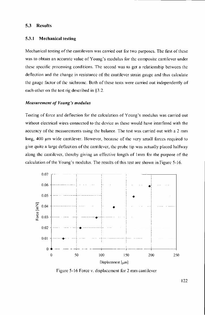
5.3 Results

5.3.1 Mechanical testing

Mechanical testing o f the cantilevers was carried out for two purposes. The first of these

was to obtam an accurate value o f Young's modulus for the composite cantilever under

these specific processing conditions. The second was to get a relationship between the

deflection and the change in resistance o f the cantilever strain gauge and thus calculate

the gauge factor o f the nichrome. Both o f these tests were carried out independently o f

each other on the test rig described in §3.2.

Measurement of Young's modulus

Testing o f force and deflection for the calculation o f Young's modulus was carried out

without electrical wires connected to the device as these would have interfered with the

accuracy o f the measurements using the balance. The test was carried out with a 2 mm

long, 400 |um wide cantilever. However, because o f the very small forces required to

give quite a large deflection o f the cantilever, the probe tip was actually placed halfway

along the cantilever, thereby giving an effective length o f 1mm for the purpose o f the

calculation o f the Young's modulus. The results o f this test are shown in Figure 5-16.

0.07 J

0.06 -

0.05 -

0.04 -

a> o 0.03 -

0.02 -

0.01 -

0 i 50 200 100 150

Displacement [|am]

Figure 5-16 Force v. displacement for 2 mm cantilever

250

122

The straight line linear best fit o f this data is

V = 2.92x]0^' 'x 5-36

And therefore the gradient o f this line is 0.3 N/m. Based on [61], Young's modulus can

be calculated as

E = ^ 5-37 35/

where F is the point load applied, L is the length of the cantilever, 5 is the tip deflection

and / is the second moment o f area o f the cantilever. For a cantilever o f the dimensions

given above and a thickness o f 12 jam this means that the Young's modulus can be

calculated as 1.69 GPa.

However because the root o f the cantilever is widened in order to avoid stress factures

forming during the fabrication process, and also because the body o f the device is not

fixed at exactly the root o f the cantilever, this value slightly overestimates the true value

of the Young's modulus o f the structure. Consequently FEA was used to achieve a more

accurate interpretation o f the force-deflection curve. This modelling was carried out

using Strand? with a non-linear solver due to the large deflection. The original

calculated value was used as an initial value and then an iterative process was used until

the correct value was found. The initial value o f Young's modulus was used to run the

model and obtain a tip deflection for the applied force. Based on this result the Young's

modulus given as a material property was then increased or decreased until the correct

tip deflection was seen.

123

The mesh used for the calculation is shown in Figure 5-17.

Figure 5-17 Mesh used for FEA modelling o f Young's modulus

The load was applied as a pouit load at the centre o f the cantilever width and 1 mm

along from the root. This is the most accurate representation o f the load applied by the

probe tip on the test rig. The deflected model for the fmal iteration is shown in Figure

5-18 with the real deflection shown.

EnclcDispDYW

0 00M96 [Bk:17821

I I

0 000397

0 000323

0.000248

0000174

0 000099

0000025

0.000000 (Bk.2902)

Figure 5-18 Model with load applied for calculation o f Young's modulus

124

This represents a load o f 0.059 mN which gives a deflection o f 196 (im halfway along

the cantilever at a position o f I mm. This is the deflection seen for the same applied

force when carrying out experimental testing. The results from the FE analysis are

shown in Figure 5-19.

0.0005

0.0004

E 0.0003

0) 0.0002

0.0001

0.0000 0.0000 0.0004 0.0008 0.0012 0.0016 0.0020

Distance (m)

Figure 5-19 Deflection v. distance along cantilever for calculation o f Young's modulus

For this result a Young's modulus o f 1.45 GPa was used for the calculation. This is

subsequently the value that has been used in all other calculations where knowledge o f

Young's modulus has been required. As expected, this value was slightly lower than

that obtained by using simple beam theory to calculate the Young's Modulus due to the

presence o f the widened anchor. This value o f Young's modulus is quite low compared

with published data for SU-8 (1.54 - 7.5 GPa [69, 71]), but within the same order of

magnitude and is the value for the composite SU-8/NiCr cantilever. However, since the

bulk Young's modulus o f nichrome is two orders o f magnitude greater than that o f SU-

8, the presence o f the thin fdm on the surface o f the cantilever would be expected to

increase the modulus o f the composite, rather than decrease it, so the actual Young's

modulus for the SU-8 alone may be lower than this calculated value. Conversely the

thickness o f the NiCr film is two orders o f magnitude less than that o f the SU-8

cantilever and consequently its effect on the stiffness o f the cantilever may be minimal.

Measurement of Gauge Factor

Mechanical testing was carried out to find the relationship between deflection and

resistance change. For the purposes o f this test, electrical connections were made to the

125

two contact pads closest to the strain gauge. They were not connected as for wind tunnel

testing o f the device where the Wheatstone bridge was utilised. The result o f this

connection was that the resistance was in fact being measured in parallel with the other

three resistors in series, as shown in Figure 5-20. The reason for this method o f

coiinection was that the test rig was set up for the measurement o f resistance rather than

to supply a vokage and then read a voltage as output as would be the case i f the

Wheatstone bridge were used.

Cantilever

Figure 5-20 Measurement o f resistance o f strain gauge

This test was undertaken for all three lengths o f cantilevers. However, the results from

the shortest, 2 mm cantilevers were found to give the most reliable results. The results

for one o f these 2 mm cantilevers are shown in Figure 5-21. The electrical connections

shown in Figure 5-20 were taken into account during the calculation o f the cantilever

output. The initial resistance o f all four resistors was measured, which in all cases was

again measured as in Figure 5-20. The actual component value of each resistor could

then be calculated and used for the determination o f what the cantilever output voltage

would be for a supply voltage o f 1 V.

126

These results are shown in Figure 5-21.

> 0.4

100 500 200 300 400

Tip deflection [|im]

Figure 5-21 Cantilever output as a function o f tip deflection

This data shows a deflection of 9.6x10"' (mVA^)/fim.

600

Thus

| / , „ = 9 . 6 x l O - V , , , ^ 5-38

where the output voltage is in mV, the input voltage is in V and d, the tip deflection, is

in | im.

From this result it was possible to calculate the gauge factor o f the nichrome. For this

case, the FE model was used to calculate the strain along the surface o f the cantilever.

This strain combined with the measured change in the resistance allowed the gauge

factor to be calculated, since

A/?/ K = 5-39

Where K is gauge factor, e is strain and R is resistance.

127

For this case, the tip deflection from the FE model could be used to give the expected

output in mV/V from equation 5-38. This can then be used to calculate the change in

resistance in the strain gauge for a known Wheatstone bridge configuration, since from

rearranging equation 5-7

^-

when all resistors in the Wheatstone bridge have the same resistance.

The strain data from the same case was then used to calculate the gauge factor using

equation 5-39. This calculation yielded a gauge factor for the nichrome strain gauge o f

1.8. This is lower than the bulk gauge factor o f 2-2.5. However, Kazi et al [79], found

that for a f i l m o f this thickness (125 nm) a gauge factor o f approximately 1.3 was seen,

with the gauge factor decreasing for f i lm thicknesses between 20 and 150 nm. The films

in this study were aimealed, however, which could account for the difference in values.

5.3.2 F E A results

The cantilever was modelled with a range o f pressures applied to the under-surface o f

the cantilever. The Young's modulus as calculated previously in §5.3.1 was used as the

material property required by the model. The tip deflection was obtained from the

model for a given pressure difference. The mesh used was the same as that for

calculating the Young's modulus and is shown in Figure 5-17. However instead o f

using a point load at the 1 mm position on the cantilever, a uniformly distributed load

was applied over the whole under-surface o f the cantilever.

128

The results o f this modelling are shown in Figure 5-22.

^ 600

0 20 40 80 100 120 60

Pressure [Pa]

Figure 5-22 Tip deflection for 2 mm cantilever vs pressure difference across cantilever

At low pressures as shown in Figure 5-22, the relationship between pressure and tip

deflection is found to be linear. At higher pressures, the relationship deviates from the

linear relationship due to the large deflection o f the cantilever.

5.3.3 C F D results

Thermal heating effects

The thermal heating effects o f the resistor were quantified by a series o f tests carried out

by CFD. It was found to be impossible to measure the degree o f heating o f the sensor

experimentally. At low supply voltages a FLIR thermal camera was unable to measure

the difference between the nichrome strain gauge with power and with the power supply

switched off, due to the small temperature difference. It was not possible to measure the

absolute temperature o f the strain gauge and the surrounding SU-8, as the different

emissivities o f the two materials meant that the two materials showed up as being at

different temperatures even when they were both at room temperature. The size o f the

129

strain gauge made it impossible to measure the temperature using such means as a

thermocouple. Consequently CFD was used to estimate the temperature reached by the

sensor under operating conditions so that the effect on the resistance change and thus

the vokage output from the sensor could be calculated.

This was done by applying a temperature to the exterior surfaces o f the sensor in the

CFD model and then running simulations at a range o f different freestream velocities

(0-20 m/s at 5 m/s intervals) and obtaining as an output from the model, the heat flux

from the sensor. This could then be compared with the known power output from a

resistor (which causes resistive heating) and, by an iterative process, the temperature

reached by the sensor could be calculated (for a known supply voltage (and therefore

heat flux) and a known freestream velocity). The results o f these simulations are shown

in Figure 5-23.

0.0035

0.003

0.0025

^ 0.002

0.0015

0.001 1

0,0005 -

— 0 nVs

^ 5 nVs

>- 10 m/s

>- 15 m/s

- 2 0 m/s

1.2 1.4 1.6

A T [ K ]

Figure 5-23 Heat flux against temperature for freestream velocities between 0 and

20 m/s

It can be seen that in this range for small values o f temperature difference the

relationship between AT and the heat flux is linear. For a supply voltage o f I V for the

four resistors o f the Wheatstone bridge, each with a nominal resistance o f 5 kQ, the

130

power dissipated is 0.8 mW. At 20 m/s this power would cause the resistor to heat by

approximately 0.4 K above ambient. This would cause a change in the resistance o f

0.06 Q, equating to an effect on the sensor output o f 0.003 mV/V. This is small

compared with the expected response caused by the pressure-induced deflection o f the

cantilever (0.75 mVA^). At zero velocity the heating effect is greatest as there is no

cooling airflow passing over the sensor causing the temperature to be higher.

The ratio o f Q/AT can be plotted against velocity which gives a relationship which

could then be used to compensate for the temperature differences at a known velocity.

This relationship is shown in Figure 5-24.

0.0025

3E -06X + 0J0002X + 0 .0002

= 0 i 9 9 2 5

0 .0015 '

< a 0,001

0.0005

0 20 25 5 10 15

V [iWs]

Figure 5-24 Ratio o f g / A T against velocity derived from CFD

The ratio o f convective heat transfer to conductive heat transfer is described by the

Nusselt number which is defined as

Nu = hi

5-41

where h is the heat transfer coefficient in W/m'K, L is the characteristic length in m and

k is the thermal conductivity o f the fluid in W/mK.

131

Since the heat transfer coefficient can be written as

AT.A 5-42

this can be substituted in to equation 5-41 to give

Nu = QL AT.k.A

5-43

Since for the temperatures being used here the Prandtl number (which is the ratio o f

momentum diffusivity and thermal diffusivity) is constant for air (usually 0.713 at

20 °C) then we can expect a relationship o f the form:

5-44

where a and b are constants, and Re is the Reynolds number.

Hence, i f the Nusselt and Reynolds numbers are calculated for the above data and the

logs o f these results are plotted, then there should be a linear relationship between the

two variables. These results are plotted in Figure 5-25.

2.05 I

2 -

1,95

1.9

I 1.85

.75

1.7

1.65 ^ ~

y = 0.494X + 0;3013

r ' = 0.9996

2.7 2.8 2.9 3 3.1 3.2 3.3 3.4 3.5

log(Re)

Figure 5-25 log(Nu) v log (Re) for heat loss from cantilever sensor

132

It can be seen that this gives a linear relationship as expected. The characteristic length

that has been used is the length o f the cantilever sensor, which is 2 mm. The constants

thus calculated as in (5-44) are a = 2.00 and b = 0.494. For forced convection over a flat

plate in a laminar boundary layer, the heat transfer conelation is given by [82] as

M / = 0.664 R e ° ^ P r " " 5-45

akhough in this case as Pr is a constant this simplifies to the form given in (5-44). It can

be seen that the power to which Re is raised (constant b) is very close to what would be

expected. This constant remains very similar for differing cases o f forced convection

over a flat plate, while the constant a varies depending on the particular configuration

and hence has not been compared here.

Effect of incidence angle

Because the cantilever deflects in the airflow before reaching an equilibrium position

the cantilever was modelled at a variety o f different incidence angles in order to

ascertain the effect that this has on the pressure drop across the cantilever. The

cantilever was modelled as a straight structure as this was easier to model in Gambit and

was expected to give a representative resuk. The exact shape o f the cantilever was

found to vary between different devices and was very diff icult to measure accurately.

The simulations were carried out at seven different incidence angles (0°, 5°, 15°, 30°,

45°, 60°, 75°) and four different velocities (or Reynolds numbers) for each angle ( f rom

5 to 20 lu/s at 5 m/s intervals). A l l simulations were carried out for a 2 mm, 400 | im

cantilever. Although the width o f the cantilever might be thought unimportant for a 2D

model, it is critical for obtaining the correct forces generated on surfaces. A boundary

layer profile was used at the inlet to the CFD domain which varied for the specific

freestream velocity. Examples o f the static pressure contours from these simulations at a

velocity o f 15 m/s are shown in Figure 5-26 to Figure 5-31 over the next three pages.

The colourbar scale has been maintained the same for all plots to allow comparison o f

the static pressure drop across the cantilever.

133

Static pressure [Pa]

1.15efD2 -9 .32et01 -7.158^01 -4.96e->Dl -2.8C et-01 -6.25e+00 l,56e+01 S.OOefOl

Figure 5-26 Static pressure contours for incidence angle o f 0°

Static pressure [Pa]

1 . 1 5 e t 0 2 _ -9.32e+01 -7.16e+01 -4,986*01 -2.8( )e*-01 -6.25e+0O 1.65e+013.00e<-01

Figure 5-27 Static pressure contours for incidence angle o f 5°

134

Static pressure [Pa] -1.15e^02 -9.32e+01 -7,15e+01 -4,98et01 -2.80^*01 -6.25e+0O 1.56e+013.00e^0t

Figure 5-28 Static pressure contours for incidence angle o f 15"

Static pressure [Pa]

1.16e<-Q2 -9 .32et01 - 7 . t { !e+fll -4,9de-t01 -2.80e*-01 -6.25e+00 1.56e+013.0 0e*^01

Figure 5-29 Static pressure contours for incidence angle o f 30°

135

Static pressure [Pa] 1.15e^Q2 -9.32eH-01 -7.156^-01 -4 .98e4Ql -2.80et01 -6.26e+0O 1.66e+013.00e<-01

Figure 5-30 Static pressure contours for incidence angle o f 45"

Static pressure [Pa]

1.15eif02 -9.32e^01 -7.15et-01 -4.9ee:^01 -2.80e^0] -6.25e+0 0 l,65e+01 3.0 0e<-0l

Figure 5-31 Static pressure contours for incidence angle of 60°

It can be clearly seen that, as in the case o f the fence, the magnitude o f the low pressure

in the area above the cantilever is much greater than the magnitude o f the high pressure

136

in the area beneath the cantilever. The high pressure is Hmited to stagnation pressure

Cp = 1, while low pressure can go down to a value o f C? < - 3.

The plots o f static pressure indicate that for incidence angles greater than 5° there are

vortices shed from the cantilever. This is another incentive for minimising the deflection

of the cantilever upwards in the airflow, in order to minimise this behaviour of the fluid

f low as far as possible. Since a steady-state calculation has been carried out, the plots

here are an attempt to represent a steady f low for these boundary conditions, despite the

fact that in reality the f low is transient where vortex shedding takes place and thus a

fiiUy converged solution is not reached.

The moment acting on the cantilever for varying incidence angles at different velocities

is shown in Figure 5-32.

l.OE-07

9.0E-08

8.0E-08

7.0E-08

E z c 'J E o

6.0E-08 ^

5.0E-08

4.0E-08

3.0E-08

2.0E-08

l.OE-08 ^

O.OE+00

0 10 20 5(1

• 5 nVs • 10 vols • 15m/s • 20 nVs

70 30 40

Incidence angle (°)

Figure 5-32 Moment on cantilever for varymg incidence angle and velocity

It can be seen that the moment acting on the cantilever increased with increasing

incidence angle. However, at high incidence angles, as was anticipated, the rate o f

change o f moment decreased as the flow stalls, which decreased the lif t on the

cantilever. However at these high incidence angles the moment continues to increase as

137

it becomes dominated by the drag acting on the cantilever. This effect can be seen at all

velocities.

The l i f t generated by the airflow acting on the cantilever is shown in Figure 5-33.

8.0E-05

7.0E-05 -I

6.0E-05

5.0E-05

4.0E-05

3.0E-05 ^

2.0E-05

l.OE-05

O.OE+00 +—*^ •

• 5 m/s • 10 m/s • 15 m/s • 20 m/s

0 10 20 30 40 50 60 70

Incidence angle (°)

Figure 5-33 L i f t on 2 mm cantilever

It can be seen that the cantilever stalls at an incidence angle o f between 30° and 45°,

where the hft decreases rapidly. The peak hft at 30° at 20 m/s corresponds to a l i f t

coefficient o f 1.3, where this was calculated using the local velocity at a position within

the boundary layer halfway along the cantilever.

138

00

Q 4.0E-05

3.0E-05

2.0E-05

l.OE-05

The drag generated by the airflow on the cantilever is shown in Figure 5-34.

9.0E-05

8.0E-05

7.0E-05

6.0E-05

5^ 5.0E-05

i

-! •

- 4 —

:

•

•

• • . „ J i

• •

, 1

• • •

1 •

10 20 30 40 50

Incidence angle (°)

Figure 5-34 Drag on 2 mm cantilever

60

• 5 m/s • 10 m/s • 15 nVs

• 20 nVs

70

The drag on the cantilever continues to increase after the airflow has stalled. The drag

coefficient at the maximum drag at 60° at 20 m/s is 0.5, again calculated using the local

velocity within the boundary layer.

The forces have been plotted here rather than l i f t and drag coefficients because o f the

difficulty o f obtaining a realistic coefficient for an object within the boundary layer. The

velocity (Reynolds number) changes the thickness o f the boundary layer and hence the

shape of the velocity profile in the region o f the cantilever. Changes in incidence angle

also alter the position o f the cantilever in the boundary layer and therefore the velocity

and velocity gradients seen by the cantilever. These variations in velocity make it

difficult to define a useftil Hft coefficient.

139

The variations in the boundary layer at different velocities and heights are illustrated m

Figure 5-35.

5

4.5

E ^ 3.5 )-H

M 3

^ 2.5 c 3

.S

" 1

0.5

0

j

1 \

L 1 A

—-J- --j

—-J- --

Om/s

20 in/s

Boundary layer thickness

10 15 20

Local velocity (m/s)

25

Figure 5-35 Boundary layer profiles and thicknesses for varying speeds

5.3.4 Combined C F D and F E results

The results fi-om CFD o f the cantilever at varying incidence angles and velocities could

be combined with the FE resuks to predict the pressure difference and deflection o f the

cantilever for each velocity.

In FE modelling, the deflection for a given pressure difference across the cantilever is

calculated as shown in Figure 5-22. The CFD results give a pressure difference (related

to moment) for a known incidence angle (and thus deflection) as shown in Figure 5-32.

Plotting these two resuks on the same axes means that the intersection w i l l give the

pressure and deflection for a specific velocky. This is a significantly more efficient

method than using an kerative approach to the problem. Akhough k would be possible

to use CFD pressure resuks as an input for the FE model to calculate a new deflection,

which could then be reintroduced to the CFD model to give a new pressure for the FE

model - this process would then be repeated until a constant resuk was achieved.

However this approach would be computationally expensive as a large number o f

140

iterations would be required to achieve a stable result, and each C F D run at a different

deflection would require a new mesh, which is time consuming to produce. The

approach used here allows as few as tliree C F D simulations to be made.

The results for a freestream velocity of 5, 10, 15 and 20 m/s are plotted in Figure 5-36,

Figure 5-37, Figure 5-38 and Figure 5-39 respectively.

1.20

o c

t/5

• 5 in/s FE Poly. (5 m'sj

10 20 30

Deflection [|im]

Figure 5-36 C F D and F E results for 5 m/s

40

141

03

o c

I D

• 10 m/s I F E Poly. (10 nVs)

50 100 150 200

Deflection [(.im]

Figure 5-37 C F D and F E results for 10 m/s

Pi 20

a 15 •o

8 ">

y y

y ' y

\ y y

y i

^y \ ,

200

• 15 m/s F E Poly. (15 m/s)

50 100 150

Deflection [|am]

Figure 5-38 C F D and F E results for 15 m/s

250

142

o c • 20 in/s

F E Poly. (20 m/s)

0 200 400 600 800 1000 1200

Deflection [^m]

Figure 5-39 C F D and F E results for 20 m/s

The non-linearity of the F E results at high pressures only become important at the

highest velocity shown here, of 20 m/s. The deviation from linear can be seen in Figure

5-39. These graphs are combined in Figure 5-40 and Figure 5-41.

c

100

90

80

£ 70

3

Q-

60

50

40

30

20

10

0

0

1 1 1 1

j

I 1

j j

j f" 1 1

-

i__ j

-

1 1

1

4 1 j

i < *

j i

25 5 10 15 20

Freestream velocity [m/s]

Figure 5-40 Pressure difference v. velocity from C F D and F E A for 2 mm cantilever

143

As can be seen from Figure 5-40, the pressure difference across the cantilever increases

at a more than linear rate, which is to be expected. With a fixed geometry and boundary

layer profile, pressures will increase with velocity squared. Mowever the pressure

difference would be expected to increase at a rate greater than this due to the decreasing

thickness of the boundary layer and the mechanical deflection causing increased

loading.

The deflection results are shown in Figure 5-41.

900

800

700

_ 600 E

— 500 c o

400

300

200

100

0

Q

1 1 1 1

_ _ _ _.

j i t

1 1 1 1

1

j

1

1 i

1

1 i

1 1

1 1

i • 1 1

0 5 10 15 20

Freest ream velocity [m/s]

Figure 5-41 Deflection v. velocity from C F D and F E A for 2 mm cantilever

25

Since deflection and pressure have a linear relationship at lower deflections, the shape

of this graph is very similar to that of the graph of pressure.

The results from the mechanical testing of the cantilevers was used to ascertain the

change in resistance that could be expected from the strain gauge for a given tip

deflection and this was then used to calculate the expected cantilever output for a given

tip deflection. This calculation was done using the relationship between tip deflection

and sensor output in (5-38).

144

The results of this analysis are shown in Figure 5-42.

0.8

0.7

^ 0.6

E 0.5

S- 0.4 o

^ 0.3

5 0.2

0.1 4

0

4

_

1

i i

i 1 1 j 1 1 1 1 j 1

i . i 1 1 1 1

1 i

0 25 5 10 15 20

Freestream velocity [m/s]

Figure 5-42 Expected output from 2 mm cantilever using C F D and F E A modelling and

mechanical testing results

These expected outputs from the sensor are for a 2 mm, 400 \im wide cantilever, and as

such would be the lowest expected results. The longer cantilevers would be expected to

give a greater sensitivity.

5.3.5 Wind tunnel results

Effect of cantilever dimensions

Three different lengths of cantilevers and two different widths were tested in the wind

tunnel in order to establish how the sensitivity of the device changed with the geometry

of the cantilever. The results of the wind tunnel testing are shown separately for

different lengths of cantilevers.

A table of the initial tip deflections for all of the cantilevers tested is shown in Table

5-5. Sensors labelled 'A' are all from the same substrate, and sensors labelled 'B ' are all

from a different substrate. 1 and 2 denote different sensors from the same substrate.

145

Length (mm) Width (urn) Sensor Tip deflection {\xm)

2 400 A l 84

2 400 B l 68

2 600 A l 0

2 600 B l 0

3 400 A l 236

3 400 B l 41

3 400 B2 158

4 400 A l 137

4 400 A2 276

4 400 B l 140

Table 5-5 Inkial tip deflections for all cantilever sensors

Resuks for the 2 mm long cantilevers are shown in Figure 5-43 with both the 400 and

600 ^m widths. The resuks shown include mukiple tests for each sensor.

> > -*-» 3 & 3 O i-i >

1.4

1.2

1

0.8

0.6

§ 0.4

0.2

0 0

• • «

• •

V

20 25

• 2 inmx400 ^ m A l

• 2 minx400 ^imBl • 2 mm X 600 ^m A l • 2mmX600 ^ m B l

5 10 15

Freestream velocity [nVs]

Figure 5-43 Resuks for 2 mm cantilevers, 400 and 600 )um widths

The resuks are plotted against freestream velocky as this is accurately measured using

the static pressures before and after the contraction m the wind tunnel, and applying the

146

calibration as described in §3.3.1. Results for shear stress come from the Preston tube

on the plate and rely on the gradient of the boundary layer profile being constant in this

region, which therefore gives less reliable results.

It can be seen that the repeatability between different sensors is quite good and that the

varying widths of the cantilevers has a minimal effect. It is possible that the similarity

of the results between the two widths is in fact due to two compensating factors. The

wider cantilevers would be expected to have a higher average pressure under them and

hence to show a larger response, llowever the wider cantilevers also had a smaller

positive initial tip deflection than their narrower counterparts, which would imply a

smaller response and it is possible that these two effects cancel each other out.

The general shape of the response curve is not linear, but a higher order polynomial,

which is what would be expected as in Figure 5-42. At low velocities the response is

very small and this corresponds with the expected results. As the cantilevers deflect,

they see a larger force, as they are higher up in the boundary layer where the velocity is

greater. This effect is compounded by the fact that pressure increases with velocity

squared and the cantilevers deflection is a ftmction of the pressure drop across the

cantilever.

147

The results for the 4 mm long cantilevers, with a width o f 400 pm are shown in Figure

5-44.

• 4 iTnnx400 ^imAl • 4 mm x 400 |im A2 • 4 mmX 400 f imBl

20 25 0 5 10 15

Freestream vefocity fnVs]

Figure 5-44 Results for 4 mm cantilevers

It can be seen that the sensitivity is significantly increased for this longer cantilever. At

10 m/s the voltage output o f the 4 mm long cantilever is approximately six times that

for the 2 mm long cantilever.

At low velocities the shape of the calibration curve is similar to that o f the shorter

cantilevers, but as the velocity increases, the shape deviates from that which might have

been expected. This is because these longer cantilevers were observed to curve back

over the body o f the device in a semi-circular shape and thus, although the strain in the

cantilever continues to increase, the rate o f change o f that strain decreases. As the

cantilever deflects it sees a greater pressure and consequently deflects further as this

increase in pressure has a non-stabilising effect.

148

The deflection o f the cantilevers is shown in Figure 5-45. The excessive deflection in

the airflow can be clearly seen, when compared with the undeflected cantilever. This

excessive deflection is the cause o f the diminishing rate o f change of strain seen in the

graph o f results. Both the undeflected cantilever in zero airflow and the cantilever in a

20 m/s flow causing the arc deflection are shown.

a )

Figure 5-45 (a) Undeflected 4 mm cantilever; (b) Cantilever deflected in airflow

149

Where the cantilever is deflected in Figure 5-45 (b), the cantilever itself can be seen and

also the shadow cast onto the plate on which it is mounted. The sensor is mounted on

the underside o f the plate.

The results from the 3 mm long cantilevers, with a width o f 400 pm are shown in Figure

5-46.

>

O

C

3.5

3

2.5

2

1.5

1

0.5

0

• y

« »• ' 1 , ,

• 3 mm X 400 ^ m A l • 3 mm X 400 | imBl • 3 mm X 400 urn B2

25 0 5 10 15 20

Freestream velocity [nVs]

Figure 5-46 Results o f 3 mm long, 400 pm wide cantilevers

It can be seen in these results that the initial tip deflection o f the cantilever does have an

impact on its response. The two devices with similar tip deflections give very similar

results. However, the device that has a significantly lower tip deflection (Sensor B l )

than the others gives a noticeably smaller response at the same velocity. It appears that

where the initial deflection is larger, variations do not have a significant effect, but

where the deflection is small a difference is seen. This is why this effect is seen in these

3 mm cantilevers, but not in the longer 4 mm cantilevers, where the anomalous initial

tip deflection is larger (Sensor A2) than the typical deflection and not smaller.

It would also appear that the 3 mm long cantilevers are also susceptible to the excessive

arc deflection seen in the 4 mm cantilevers but not in the shortest 2 mm long

cantilevers. This is what causes the decrease in the rate o f change o f the voltage output

150

from the sensor for high velocities. However, as would be expected, the effect is less

pronounced in these shorter cantilevers.

Effect of variation of excitation voltage

The effect o f varying the excitation voltage is shown in Figure 5-47. The sensor used

for this test was a 4 mm x 400 |j.m sensor B as this sensor gave representative results for

a sensor of these dimensions.

• 0.25 V • 0.5 V • 1 V • 2 V

10 15 20 25

Freestream vebcity [m/s]

Figure 5-47 Effect o f varying excitation voltage

It can be seen that the mVA^ sensitivity o f the cantilever is independent of the supply

voltage. Increasing the supply voltage would be expected to increase the heating o f the

strain gauge and hence the thermal noise o f the sensor.

The thermal effect would be expected to be greatest at low velocities as the cooling

effect o f the airflow by forced convection has least impact and consequently the

resistive heatuig effect in the strain gauge increases the temperature o f the metal by the

greatest degree.

151

However it can be seen that the effect o f the resistive heating on the sensor output is

negHgible, as predicted by the CFD modellmg shown in §5.3.2.

Effect of variation of axial position

A 4 mm cantilever was placed at two different axial positions, 0.125 m and 0.25 m

downstream o f the leading edge of the plate, in order to subject the sensor to different

boundary layer thicknesses. The sensor used was a 4 mm x 400 fxm cantilever A2. The

results are shown in Figure 5-48.

>

3 B-3 O

>

I

3.5

3

2.5

2

1.5

1

0.5

0

• •

•

•

5 10 15 20

Freestream vetocity [nVs]

• Axial position 0.125 m • Axial position 0.25 m

25

Figure 5-48 Effect o f varying axial position, plotted against freestream velocity

These results would give a better indication o f the effect o f the axial position i f they

were plotted against shear stress rather than freestream velocity, because although the

freestream velocity remains the same regardless o f the position o f the sensor on the

plate, the shear stress changes due to the size o f the boundary layer, which at an earlier

axial position is smaller than fiirther along the plate. Therefore the shear stress as

measured by the Preston tube mounted next to the sensor is what should be compared

for the two tests.

152

These results are shown in Figure 5-49.

3.5

^ 2.5

I r 2 B-3 O

I •a c U

1.5

1 4

0.5 •

• •

>«*»• •

0.1 0.2 0.3 0.4

Wall shear stress [Pa]

• Axial position 0.125 m • Axial position 0.25 m

0.5

Figure 5-49 Effect o f varying axial position, plotted against shear stress

It can be seen that the response in this graph is the same regardless o f the position along

the plate o f the sensor, despite the relative differences in the thickness o f the boundary

layer at these positions. This means that the sensor is capable o f sensing shear stress

independently o f the shape o f the boundary layer.

Comparison of theoretical and experimental results

The results for a 2 mm, 400 micron cantilever were compared with the theoretical

results obtained from the CFD and FEA modelling; this comparison is shown in Figure

5-50. The reason for comparing data from the 2 mm cantilevers is that they do not curl

back over themselves as the longer cantilevers have shown themselves to do, which is

something which could not easily be modelled in the FE or CFD modelling and is also

an undesirable effect.

153

The results from the CFD and FEA are taken from the results calculated in §5.3.4.

> 0.8

• Experimental

• CFD and FE

5 10 15

Freestream velocity [m/s]

20 25

Figure 5-50 Comparison o f theoretical and experimental data for 2 mm cantilever

It can be seen that the experimental results do not exactly match those predicted by the

theoretical calculations, although the general trend is the same. However there are a

number o f limitations to the theoretical modelling that has been carried out which would

probably account for the differences that are seen here. The CFD modeUing has been

carried out in 2D and consequently w i l l not be entirely accurate m the prediction o f the

pressure difference across the cantilever. The most significant effect o f the 2D

modelling o f a 3D situation is that the effect o f leakage o f the flow around the edges o f

the cantilever is lost and thus the CFD results would tend to overestimate the pressure

difference across the cantilever. In addition the cantilever was modelled as a straight

structure, while in reality it was a curved structure. This would also have an impact on

the accuracy o f the pressure difference that has been calculated.

The FE modelling has been carried out in 3D and consequently should give a

reasonably accurate representation o f the bending o f the cantilever under an applied

load. In addition, the Young's modulus o f the cantilever that is used for these

154

calculations should be accurate as it has been measured experimentally for this structure

and these processing conditions. However the existing stress and internal stress gradient

in the material are not taken into account in the modelling. In addition, the transfer o f

CFD pressure data into the FE model is not detailed in that a constant pressure over the

surface o f the cantilever is assumed.

5.4 Summary

An in-plane cantilever sensor has been constructed from a composite o f SU-8 and

nichrome to measure wall shear stress. This sensor has been shown to measure

successfully the wall shear stress over a range between 0 and 0.4 Pa. It is a sensor that is

not prone to errors caused by changes in ambient temperature as it does not have high

thermal sensitivity, due to the low thermal coefficient o f resistivity o f nichrome. The

excitation voltage applied to the sensor does not have an effect on the output from the

sensor, due to the lack o f thermal heating in the resistor.

The sensor has been fabricated in a number o f different geometries so that the influence

of altering the length and width o f the cantilever could be assessed. As expected it was

found that increasing the length o f the cantilever had the effect of increasing the

.sensitivity. However, in the longest 4 mm long cantilevers it was observed that the

cantilever deflected back over the body of the sensor in an arc at higher flow speeds.

This had a detrimental effect on the designed low impact o f the sensor on the airflow.

Ideally the sensor would not exhibit this behaviour, and in effect these longer

cantilevers were too sensitive for the application for which they were being used.

Varying the width o f the cantilever did not have a significant influence on the

sensitivity o f the cantilever. It would have been expected that the wider o f the

cantilevers had a greater sensitivity due to leakage o f the airflow around the edges o f the

cantilever being more pronounced for a narrower cantilever, but this was not found to

be the case. However where edge effects do not have an effect on the flow, the

increased pressure force from the flow would be directly compensated for by the

increase in second moment o f area, suggesting that the response of the cantilevers

would not be affected by the width o f the cantilever. This is a very useful effect as the

55

width o f the cantilever can be reduced, with the limiting factor being only fitting the

strain gauge within the structure, although the aerodynamic effects o f a narrow

cantilever may become pronounced at very narrow widths.

The shear stress could be measured by the sensor independently o f the shape o f the

boundary layer when placed at different axial positions. This was ascertained by placing

the sensor at a different axial position on the flat plate and comparing its response with

that o f the Preston tube being used to measure the shear stress along side it.

Altering the excitation voltage o f the Wheatstone bridge was not found to have any

influence on the response o f the sensor. This means that the sensor is not affected by the

heat generated in the resistors. This was as predicted by the thermal CFD modelling.

The cantilever was not seen to resonate at its natural frequency, which means that the

unsteady structures within the flow did not have an influence on the response o f the

cantilever, suggesting potential for high frequency measurements. However work done

here was carried out in a laminar boundary layer, and the cantilever would be more

likely to resonate in a turbulent flow.

One alteration to the current device could improve it in several ways. Making the sensor

from a combination o f silicon with a doped silicon piezoresistor instead o f the current

polymer/metal combination would have a number o f advantages. One o f these would be

that while the sensitivity would remain approximately the same due to the high gauge

factor o f doped silicon [63], but the higher Young's modulus of silicon would mean that

the cantilever would deflect far less for the same force. The consequence o f this would

be that the cantilever would have significantly less impact on the airflow, and would

probably remain within the laminar sub-layer o f the boundary layer, which would be a

great advantage. In addition, the increased Young's modulus would also have the effect

o f increasing the resonant frequency o f the cantilever, which would be an advantage

despite resonance not being seen in laminar testing. Although steady state

measurements have been carried out in this work, in order to make transient

measurements it would be an advantage to have a sensor with a higher resonant

frequency as it would be less affected by turbulence within the airflow.

156

Chapter 6

3D flow vector measurement

In this work the design and manufacturing process o f the cantilever shear stress sensor

was adapted for use in the measurement o f freestream velocity vectors. Four sensors

arranged in an orthogonal manner around a square section mounting allowed 3D flow

measurements to be taken. The airflow probe was modelled using CFD and FEA and

then two different designs o f probe were tested in the wind tunnel.

6.1 Background

The desirable features o f a probe for measuring freestream velocity vectors were

described in §1.1. The principle objective in this part o f the project was to demonstrate a

MEMS probe design able to achieve tip dimensions smaller than the current available

minimum of approximately 1 mm diameter. The MEMS probe was designed to give the

same information as that available when using a five-hole probe, due to the existing

mathematical parameters and experimental infrastructure for calibrating probes of this

type. Additionally this type o f probe is a commonly used and understood method o f

taking point measurements o f velocity vectors making it a good basis for a new design.

157

A five-hole probe measures yaw, pitch, and dynamic and stagnation pressures. These

are calculated from the yaw and pitch coefficients as well as the dynamic and stagnation

pressure coefficients, which are obtained by calibration o f a specific probe. There are

different methods o f defining these coefficients for a 5-hole probe, but those used at

Durham University are presented here [83].

The holes are numbered as shown in Figure 6-1. Positive yaw is defined as an increase

in pressure on hole 1, and positive pitch as an increase in pressure on hole 3.

+ve pitch

+ve yaw

Figure 6-1 Five-hole probe numbering (view onto probe head)

The coefficients for a five-hole probe are calculated as follows:

Yaw coefficient was defined as

where PQ, PI and P2 are the pressures recorded at holes 0, 1 and 2 respectively, and Pav

is defined as

Pitch coefficient was defined as

^P„ch - p _ p

158

The Dynamic pressure coefficient was defined as

Corn - — 6-4

where P^/y,, is the dynamic pressure

and the stagnation pressure coefficient as

Cp 6-5

where P,o, is the total pressure.

The definitions o f corresponding coefficients for the MEMS probe were intended to be

based on the above definitions for a 5-hole probe.

6.2 Theory of operation

The new probe design was intended to use similar methods o f calculating the

coefficients, and thus required a similar set-up with some devices sensitive to yaw and

others sensitive to pitch, where the response o f all o f the sensors combined could be

used to normalise the response o f the two pairs. In addition, to allow the measurement

of pressure, a hole for measuring the stagnation pressure at the probe tip needed to be

incorporated into the design. This would allow the calculation o f the stagnation pressure

coefficient. The dynamic pressure coefficient could be obtained from the response o f all

four sensors, as were used to normalise the responses for the yaw and pitch coefficients.

Using multiples o f the cantilever shear stress sensors it was possible to measure the

velocity vectors. Rather than mounting the sensor on a surface in order to measure the

shear stress, the sensors were mounted on a specially designed probe head. Four o f them

were mounted at 90° to each other. Although theoretically three sensors could be used

to obtain the three velocity components, the diameter o f the probe tip was not made

larger by using four sensors, and therefore it was decided to build some redundancy into

159

the system. This mimics the structure o f a five-hole probe as opposed to that of a four-

hole probe i f only three o f the cantilever sensors were used.

A possible arrangement o f the probe sensors is shown in Figure 6-2. The two pairs o f

sensors to measure yaw and pitch are shown as well as the central hole for pressure

measurement. Strain gauges would be incorporated into the cantilever sensors as for

measuring wall shear stress, in order to measure the pressure-induced deflection.

Figure 6-2 Sketch o f probe tip and sensors

The four sensors on the probe are numbered as shown in Figure 6-3. Positive yaw is

defined as an increase in pressure on the inside surface o f sensor 1, and positive pitch as

an increase in pressure on the inside surface o f sensor 2.

+ve yaw +ve pitch

Figure 6-3 Probe sensor numbering

160

The coefficients obtained from the probe correspond to those which would be used for a

five-hole probe. The four coefficients are defined below. They are calculated from the

calibration data to produce maps o f the four coefficients for varying yaw and pitch.

When the probe is being used, the yaw and pitch coefficients can be calculated from the

experimental data to give a pitch and yaw for the probe. These values can then be used

to obtain the two pressure coefficients from the calibration which w i l l then give the

dynamic and stagnation pressures.

The assumption is that the yaw coefficient is dominated by the difference between the

two sensors normal to the yaw direction, which are then normalised by using the sum o f

all four sensors. The pitch coefficient is the same with the other two sensors which are

normal to the pitch direction.

Yaw coefficient was defined as

<-)w = -— 6-6

where K/, K?, and V4 are the voltage outputs from the sensors in mVN.

And Pitch coefficient was defined as

^ Pilch - ~ ~ ~ 0 - /

The Dynamic coefficient was defined as

_ . I - r K 3 ^Dy>,- p 0 - 8

where f ,/,.„ is the dynamic pressure.

161

The stagnation pressure coefficient was defined as

6-9

where Pi„obe is the probe pressure and Pg is the upstream total pressure.

Although the pitch and yaw coefficients are non-dimensional, the dynamic and

stagnation pressure coefficients have units o f (mV/V)/Pa and Pa/(mVA') respectively.

These coefficients would be obtained f rom calibrating the probe, and would then be

used to get the yaw, pitch and dynamic and stagnation pressures when the probe was

being used in testing. The process for this is described in Figure 6-4.

Measurements probe V , v.,

Calculate C, , , and C,„,

Interpolate for Pitch and Yaw

Interpolate for C,„„ and C,,,

Calculate P,^„ and

Results dyn Pitch Yaw

Figure 6-4 Flow chart o f the use o f coefficients for calculating variables

The main challenge with the construction of this probe was the assembly o f the four

sensors into a single probe in such a way that the electrical connections required could

162

be made. In order to attach the wires by silver paint as had been used previously, contact

pads on the order o f 2 mm across were required. This meant that the probe would have

to widen to this size at the position o f the contact pads for the Wheatstone bridge.

However, the tip diameter could still be minimised, and this was the objective here. The

angle at which the probe increased in diameter was minimised as far as possible, but the

limits o f this are the length o f the connections from the strain gauge to the contact pads

compared with the length o f the actual strain gauge in the cantilever itself

6.3 Design and Fabrication

6.3.1 MEMS Fabrication

The aim was to use as similar a fabrication process as possible for making the MEMS

devices as was used for making the cantilever shear stress sensors. This was largely

possible due to the similarity o f the sensing structure; however the device could be

simplified in some areas, which was found to increase the yield.

It was no longer necessary to incorporate a step to create the cantilever as was required

when the sensor was mounted on a surface. Instead the cantilever structure was created

by overhanging the sensing element in the way it was mounted on the probe as a whole.

This meant that the thick 100 | im layer o f SU-8 was unnecessary and could therefore be

eliminated, meaning that the number o f masks required was reduced from three to two.

In MEMS fabrication any reduction in the number o f masks is advantageous as the

probability o f defects occurring increases rapidly with each additional photolithographic

step. This is due not only to defects in the masks themselves, but also problems in

processing.

In addition, the elimination o f this step meant that the contact pads could be fabricated

on the same side o f the SU-8 layer as the strain gauge meaning that there was no longer

a requirement to have good step coverage when depositing the nichrome, as this step

could be eradicated. Since the nichrome would therefore no longer be deposited directly

onto the sacrificial layer, this also simplified the release method allowing the device to

be fabricated directly on Prolifl without the overlying layer o f titanium required for the

fabrication o f the shear stress sensors.

163

The layout o f the probe sensor is shown in Figure 6-5.

Contact pads

Strain gauge

0.4 mm

Cantilever sensor Wheatstone bridge resistors

Figure 6-5 The probe sensor

The strain gauge in the cantilever section can be seen as well as the other resistors o f the

Wheatstone bridge. Because o f the need to make the diameter o f the probe as small as

possible, the layout is constrained to this elongated design. The contact pads are 2 mm

square and the width o f the section containing the contact pads is 3 mm to allow room

for the resistors which make up the Wheatstone bridge. This is one o f the four sensors

that together make up the probe.

The fabrication flow for the probe sensors is shown in Table 6-1.

a) A Prolitt layer is spun onto the silicon wafer

to act as a final release layer.

b)

/ / / / / / / / /

A 10 )am layer of SU8 is then spun on, and

patterned.

164

A 125 nm nichrome layer is then deposited by

sputtering, which is then patterned using a

/ / / / / / / / / / standard photolithography process, and the

exposed areas are etched.

^ The Prolift layer is then etched in T M A H to

release the devices.

Table 6-1 Fabrication flow for probe sensors

This fabrication process is significantly simpler than that required to manufacture the

cantilever shear stress sensor, which is a significant advantage for increasing the yield

o f successfijl sensors from each substrate. However, the devices were found to be quite

fragile after release and care was required to avoid tearing them. It was possible to

handle them with tweezers, however, and once mounted on the probe head this fragility

became less o f a problem.

6.3.2 Probe assembly

The probe was assembled from the MEMS devices mounted on to a probe head,

produced using a rapid prototyping machine (Objet Eden500V). The smallest resolution

nominally achievable using this machine is 0.5 mm, i.e. a 0.5 mm thick wall and a

0.5 mm hole through the material. The problem with achieving very small holes is

clearing support material from the hole afterwards. Because o f the intention to have a

hole through the centre o f the probe for measuring total pressure, and to keep the probe

tip as small as possible, four different sizes o f probe heads were designed, ranging from

the largest which had an achievable 0.5 mm wall with 0.5 mm hole, which would thus

result in a 1.5 mm total diameter, to the smallest with a total tip diameter o f 0.5 mm,

with the walls and hole equally spaced, which had an excellent tip diameter, but might

165

not be achievable using the rapid prototyping machine. A picture o f the probe head with

a 1 mm tip diameter is shown in Figure 6-6.

Figure 6-6 1 mm tip diameter probe head

The boss seen at the right hand end o f the picture is inserted into a stainless steel tube

100 mm long, which has a standard fitting on the other end for use in Durham wind

tunnels. Since this tube and the fitting are hollow, this allows the hypodermic tube for

measuring the pressure to be passed through it for access to a pressure transducer.

Alternatively a compact transducer could be incorporated into the probe head.

It was found that the minimum size which could be successfully produced using the

rapid prototyper had a 1 mm total tip diameter, with 0.33 mm walls and a 0.33 mm

diameter hole. For structures smaller than this the tip was found to have insufficiently

precise edges, which was unacceptable since this forms the root o f the cantilever when

the MEMS devices are attached.

The MEMS devices were attached to the probe head using U V curable glue. The

advantage o f this type o f glue was that as the probe was being assembled in the clean

room, in yellow light, the device could be repositioned as necessary to allow for

accurate alignment without the glue starting to set. The glue was then cured using a

mask aligner, which allowed rapid curing once the device was in position. The device

was exposed to U V light for minutes which was found to be sufficient to cure the

glue. This method was possible because SU-8 is transparent. Under the contact pads the

U V Ught could not penetrate through the nichrome layer, however there was found to be

sufficient area around the edges o f these pads for adhesion.

166

The MEMS devices were glued on to the probe head one at a time. This allowed them

to be accurately aligned individually without interfering with devices aheady attached,

as once the glue had been cured on one side this device was immovable.

A cross-section through the probe after the sensors have been mounted is shown in

Figure 6-7.

Pair of sensors RP probe head

0.5 mml[

Sensor

Pressure hole Inserted into steel tube

Figure 6-7 Cross-section through probe (not to scale)

A photo o f the four devices mounted on the probe head is shown in Figure 6-8. The

sensors on two sides o f the probe are shown here. Because o f the design o f the probe

mounting, the sensors converge, resulting in a smaller probe tip than would be the case

i f the sensors were parallel.

1 i

• • • i

Figure 6-8 The four probe sensors mounted on probe head.

Damage can be seen on the contact pads in Figure 6-8. This was caused by measuring

the resistance o f the strain gauge prior to mounting the sensors on the probe head. This

damage was not a problem for connecting the wires to the contact pads.

167

A close up photograph o f the probe tip and the orientation o f the cantilevers is shown in

Figure 6-9.

Protrud

Figure 6-9 Close up o f probe tip

The four cantilever sensors can be seen at the tip. The channel running though the

translucent probe head material can be seen behind the resistor wires running towards

the contact pads on the closest face.

The probe head did not have perfectly precise edges at the tip even with this 1 mm tip

diameter and this can be seen in Figure 6-9. This means that the degree of overhang for

each o f the cantilever sensors could be different which would mean that the response o f

the probe would not be symmetric.

Once the four devices had been attached, the next step was to attach a hypodermic tube

into the end o f the probe head for attaching to a pressure transducer. This was done

using Araldite, being careful not to block the hole. At the tip o f the probe, the diameter

o f the hole was only 0.33 mm widening to 2 mm once the probe head was wide enough

to allow this, and this was where the hypodermic is inserted. The external diameter o f

the hypodermic tube was 1.24 mm.

168

The probe head was then mounted into the stainless steel tube before the wires were

attached to the contact pads due to the risk o f dislodging the wires while handling the

probe i f this were done the other way round. Whilst ensuring a good electrical contact,

silver paint does not allow a large force to be applied to the connection without failing.

Eight twisted pairs o f wires were required for connections to the four Wheatstone

bridges. These were secured by double-sided tape where the probe head was inserted

into the steel tubing in order to minimise the pressure put on the connection.

6.4 Results

6.4.1 F E M results

The probe cantilever was modelled simply as a cantilever with a fixed end, because the

geometry was simpler than when the cantilever sensor was being modelled. There was

no anchor structure as had previously been used to eliminate stress fractures, as the 90°

angle which caused them was not present in the probe sensor. The same Young's

modulus was used as for the cantilever shear stress sensor.

The sensor was still modelled using the non-linear solver, although as the cantilever was

shorter the deflections were smaller. At lower pressures it was found that the strain in

the cantilever varied linearly with the pressure applied to the surface o f the cantilever.

The strain measured was on the top surface of the cantilever with the force applied to

the underside o f the cantilever, and consequently the strain was negative.

From the results o f strain in the cantilever, it was possible to calculate, for a given

gauge factor o f nichrome {K = 1.8 as calculated in §5.3.1) and a known Wheatstone

bridge arrangement, the expected output from the sensor.

169

The strain in the cantilever caused by the applied load is shown in Figure 6-10 and the

expected output from the sensor is shown in Figure 6-11.

0 r

-0.5

.s r3

1.5

-2.5

100 200 300 400

Pressiue [Pa]

500 600

Figure 6-10 Microstrain against pressure difference for probe sensor

1.2

^ 0.8

I

o

(U c/0

0.2

0 100 500 200 300 400

Pressure [Pa]

Figure 6-11 Sensor output for applied uniformly distributed load

600

170

As a result o f the linear relationship between pressure and sensor output in the relevant

range, it was found possible to convert from calculated pressure on the sensor surface to

expected sensor output by the following equation.

A ^ ' „ = 2 . 0 6 x l 0 - ^ A P 3-1

where AFvcmo/ is in mV and A/^ is in Pa.

The tip deflection was also linear with pressure. The results for deflection are shown in

Figure 6-12. It can be seen that due to the shorter length o f the cantilever, the

deflections are much smaller than those seen in the cantilever shear stress sensor.

0.3

0.25

^ 0.2

I 0.15 o (U

0.05

0 ^ 100 200 300 400

Pressure [Pa]

500 600

Figure 6-12 Tip deflection against pressure for probe sensor

6.4.2 C F D Results

The probe was modelled using CFD in order to obtain an estimate o f the pressure drop

across the sensors which make up the probe. This then allowed the response o f the

sensors to be calculated.

171

The probe was modelled in 3D because the interaction between all four sensors was

expected to have a significant effect on the pressure drop calculated across them. I f

there were no gap at the corners o f the .sensors then the importance o f this would be less

pronounced, but with their presence allowing the f low to be diverted around the sensor

it is important to model the flow in 3D.

The CFD domain was constructed to be large compared with the size o f the probe head,

in order to ensure that the boundaries of the domain did not have an effect on the flows

calculated in the vicinity o f the probe tip. Because the inlet f low was to be modelled at a

variety o f different yaw angles, it was necessary to have two sides o f the rectangular

domain as inlets, and two sides as outlets. The top and bottom faces o f the domain were

defuied as 'symmetry'. The inlet flow velocity was defined in component form in order

to allow a variety o f different yaw angles to be modelled.

The outline o f the domain used for modelling the probe is shown in Figure 6-13.

Probe tip

Inlet Body of probe

Outlet

Figure 6-13 Structure o f probe CFD domain

172

The domain was constructed in order to allow a mesh with very small cells in the region

o f interest around the probe tip, but to give a smooth graduation to relatively large cells

at the edges o f the domain. This minimised the total number o f cells, making the mesh

quicker to solve.

The origin (0,0,0) is situated at the tip o f the probe - at the end o f the probe cantilevers,

which is the smallest part o f the probe.

The mesh that was created was checked to ensure that the results were not mesh

dependent. Increasing the number o f nodes in the mesh edges by 20% was found to

have no significant effect on the results o f the static pressures on the surfaces o f the

sensors, but caused a large increase in the computational time required to solve the

mesh.

The pressure tapping was represented by a recess I mm deep was set into the face o f the

tip o f the probe in order to accurately model the pressure that would be seen by the

pressure transducer connected to the probe. However, although in reality this hole was

circular, in CFD it has been modelled as having a square cross-section in order to

facilitate meshing the model with a structured grid. This would not be expected to have

any significant effect on the pressure calculated.

The mesh remained the same with different inlet velocities and incidence angles being

applied. Runs were done at 10 m/s and 20 m/s for incidence angles of 0 to 50° at 10°

intervals. These velocities represented Reynolds numbers in the region o f 1000, using

the tip diameter o f the probe as the representative length, and thus a laminar model was

used. The pressure difference across all four sensors was calculated as well as the

pressure measurement from the probe.

173

The pressure drop across the sensors for varying yaw angles is shown in Figure 6-14.

s

a &

o

0 0

400

300

200

100

0

-100

-200

-300

-400

-500

• •

•

• ^ .

:

P •

L\ 2 [) 4 6 i

•

< •

1

i L ^ .

• Sensor 1

• Sensor 2

• Sensor 3

• Sensor 4

Yaw angle ["]

Figure 6-14 Static pressure drop across all four sensors at 20 m/s for varying incidence

angles

The two sensors parallel to the flow direction (2 and 4) were found to have the same

response due to the symmetrical nature o f the probe. This response was not found to

alter significantly as the yaw angle increased. This was as expected since these two

sensors would be expected to be sensitive to pitch, not yaw. At zero incidence, all four

o f the sensors deflected outwards, but once the incidence angle was increased, the

sensor closest to the flow was found to deflect inwards. At very high incidence angles,

above 50 °, this sensor partially occluded the flow onto the sensor on the opposite side

causing the pressure difference across this sensor to decrease.

Maps o f the static pressure around the probe tip for cross-sections through the centre o f

the domain in the horizontal and vertical planes for different incidence angles are shown

in Table 6-2, spread over the next two pages. The flow incidence is varied in the

horizontal plane, corresponding to yaw angle.

174

Incidence Horizontal plane

angle ["]

Vertical plane

0

10

20

Static pressure [Pa] - l , 2BBfD2 - 7 . 1 2 e » a i - I . ^ B E ^ O I I . S O e - O l Q.BBe'Ql 1.55e'a2 2 . 1 2 e » 0 2 2 . 5 0 E ' a 2

Static pressure [Pa] -1.2lB^D2 -B.B2B-Q1 - l , 4 9 e ^ 0 l 3 .B3e»01 Q. lBe 'Ol 1.45B'02 1.9Be'a2 2.a4B'a2

Static pressure [Pa] - 2 , 3 7 B » 0 2 - 1 , 8 4 6 * 0 2 - 9 . l 2 B ' - a i - 1 . 6 3 E » 0 1 5 ,47E'01 1.266-^02 2.01 E ^ O 2 2.49B'-a2

175

30

40

Static pressure [Pa] - • . l O e ' O E - 3 . I 0 B - 0 2 - 2 . i a B < - 0 2 - l . l Q e ' O E - 9 , 7 3 B ' - 0 a a . a a e ' O l 1.90e-^Q2 S . S Z B ' Q S

Static pressure [Pa]

50

5 . 9 9 E - Q 2 -4,72e<-02 -3.45B<-a2 - 2 . 1 9 B ' a 2 -9.20 B - a i iA7B'a\ l . B l e ' ' a 2 2 . 4 B B

Static pressure [Pa B ' O E - B . 2 4 B « - 0 2 -4 .7BE>-a2 - 3 . 2 B B ' 0 2 -i.ao 6 ^ 0 2 - 3 . 1 7 E ' a i l . l B e - a Z Z . l S i

Table 6-2 Static pressures for varying incidence angles

It can be seen that the flow in the vertical plane remains fairly constant as the angle o f

the flow remains the same in this plane. However in the horizontal plane, as the

incidence angle increases, the pressure on the sensor at the outside o f the probe tip

increases and on the far side from the f low inlet, the pressure drop behind the sensor is

176

more pronounced. The pressure measured at the pressure tapping, which in the CFD

model is represented as a recess between the sensors, can be seen to decrease as the

incidence angle increases, and to be negative at higher incidence angles.

From the FE results and mechanical testing, it was possible to convert the static pressure

drop into the expected sensor output from each of the four sensors. These results are

shown in Figure 6-15.

1

0.8

0.6

^ 0-4

> 0.2

:3 -4—>

o o G (U

GO

0

-0.2

-0.4

-0.6

-0.8

-1

I

<

I I 1 1 « > *

11 1 n 2h 1 0 .4 ) 5 3 6 •

i 1 1 1

1

1

1 f 1 1 1

• Sensor 1

• Sensor 2

• Sensor 3

• Sensor 4

Yaw angle [°]

Figure 6-15 Sensor output for each sensor at varying incidence angles from modelling

The results from the CFD modelling were used to assess the calculations o f yaw

coefficient, pitch coefficient, dynamic coefficient and the stagnation pressure

coefficient.

These are the coefficients as they would be calculated from wind tunnel calibration data

(defined in §6.2). For these to be calculated from the theoretical results the pressure

drop across the cantilever was converted into the expected voltage output from the

sensor in mVA''. However since this relationship was found to be linear, this was

actually unnecessary for calculating the pitch and yaw coefficients, but would have an

effect on the pressure coefficients.

177

Since only yaw was modelled in the CFD simulations, the pitch coefficient was not

calculated. The yaw coefficient is shown in Figure 6-16.

C o

I

0

-2

-4

-6

-8 -

-10

-12

-14

IP 2t) 3p 4D 5b

• 20 m/s Re = 1340

• 10 nVs Re = 671

• 10 m/s Re = 1340

Yaw angle ["]

Figure 6-16 Yaw coefficients at varying incidence angles at 10 and 20 m/s

It can be seen that at increased incidence angles the calculated yaw coefficient is not

independent o f velocity as would be expected. However this discrepancy can be

attributed to sensitivity to Reynolds number. This was confirmed by redoing the runs at

10 m/s, but halving the viscosity in order to artificially maintain the Reynolds number at

the same value as the runs at 20 m/s. Altering the viscosity in order to achieve the same

Reynolds number results in the same yaw coefficient at the two different velocities. At

very high yaw angles, the negative pressure on the sensor closest to and normal to the

flow dominates the positive pressures on the other sensors with the result that the sum

o f the pressure on the sensors (which is used to non-dimensionalise the pitch and yaw

coefficients) becomes very small and eventually negative. This has the effect o f driving

the coefficients very large before they suddenly become negative. It is at this point that

the probe can be considered to be out o f range.

178

The pressure measured by the centre pressure tapping in the probe was also obtained

from the CFD simulations. These results are shown in Figure 6-17.

3

o

300

250

200

150

100

50

0

-50

-100

-150

-200

1 l' 1 1

1 1

1 1-*-

j

1 1 1 1 1 I

1 1

1 1 1 1

1 1 1

1 1 i 1 1

W" 1 1 1

1 j

i ^ 1 1 1 1

I

1 1 1 1

LL lb_ TIO 3 1

1 41) 5 1 1 1 1

1 1 1

1 1 1

1 1 1

1 1 1 1 1

1

W

Yaw angle ["]

Figure 6-17 Centre hole pressure at varying incidence angles at 20 m/s

As expected, at zero incidence the value o f this pressure is approximately the dynamic

pressure. However as the incidence increases the pressure measured decreases until, at

angles above 30", the pressure becomes negative, i.e. is below freestream static

pressure. This effect is altered by the presence of the sensors interrupting the flow

before it reaches the pressure hole.

In order to establish the effect o f the sensors on the pressure seen by the probe, the

simulations were re-run with the sensors removed.

179

The results from this are shown in Figure 6-18 along with the original results with the

sensors present. It can be seen that the probe pressure is much higher when the sensors

are not present as they do not obstruct the airflow into the pressure tapping hole.

300

250

200

150

100

50 a . 0 \

-50

-100

-150

-200

.20-

• Sensors

• No sensors

do

Yaw angle [°]

Figure 6-18 Probe pressure at varying incidence angles at 20 m/s with sensors and in

absence o f sensors

The stagnation pressure coefficient calculated from this pressure is shown in Figure

6-19.

c OJ

0) o o

o

G TO

GO

500

0

-500

-1000

-1500

-2000

-2500

-3000

1

a J . I » i

, ._ 1

1

1

• •

0 10 20 30 40 50

Yaw angle ["]

Figure 6-19 Stagnation pressure coefficient for varying incidence angle

180

As was expected, the stagnation pressure coefficient decreased with increasing

incidence angle. The coefficient would always be negative as the probe pressure is

referenced to total pressure.

The dynamic pressure coefficient was also calculated and is shown in Figure 6-20.

>

C

o o

Q .

o s C

> Q

0.0018

0.0016

0.0014

0.0012

0.001

0.0008

0.0006

0.0004

0.0002

0

1 1

1 i i 1 1 1 1 I 1 1 1 1 1

1 1 ' 1

•

w

1 1

20 30

Yaw angle ["]

40 50

Figure 6-20 Dynamic pressure coefficient for varying incidence angle

The dynamic pressure coefficient decreases slightly at increasing yaw angles, as would

be seen when using a 5-hole probe.

181

6.4.3 Wind tunnel results

The probe was mounted in the probe cahbration test rig for airflow testing. The probe

and test rig are shown in Figure 6-21.

Figure 6-21 Probe mounted in probe cahbration test rig

The probe is mounted in the test rig and the four Wheatstone bridges are connected up

to the voltage supply and the DAQ. The same voltage supply was used for all four

bridges with them connected in parallel, since the current demand in each bridge is very

low. The probe pressure is connected to a pressure transducer, referenced to the

upstream total pressure and a second pressure transducer measures the static pressure,

also referenced to the upstream total pressure. Both these pressure transducers are also

connected to the DAQ. Also measured by the DAQ was the input voltage to check

whether this supply voltage varied with time. Further details on the probe calibration

test rig were given in §3.3.1.

182

The probe is shown in close up in Figure 6-22.

Figure 6-22 Probe and mountings for accurate angular displacement

The wind tunnel was set to a constant velocity for a series o f tests to be completed. A

range o f different angles to the flow were applied, with measurements o f the voltage

output from the Wheatstone bridge taken at each position. The stepper motors allowed

the angle at which the probe was positioned to be set accurately.

The raw data from these tests were analysed to give results in mVA^, which are

normalised for the input voltage. These results would then be used for the calculation o f

the coefficients used to define the behaviour o f the probe. Maps o f the coefficients

could then be plotted for a range o f pitch and yaw angles, which would then be used as

calibration maps for the probe. The coefficients calculated could then be compared with

those expected from the theoretical data.

Due to the difficulties in reliably assembling a probe with all four sensors electrically

connected, a probe with a single sensor which was fliUy fiinctional was used for

183

measurements. The other three sensors were all mounted on the probe head, which was

important for the aerodynamic response, but were not electrically cormected.

The results for two sensors. Sensor 1 and Sensor 2 (for definitions see Figure 6-3) to the

f low are shown in Figure 6-23 for varying yaw angles.

0.25

0.2

0.15

I 0.1

(D

0.05

0

•0.05

-0.1

•0.15

\

i ; ;•

\ -

\ • I *

• :

\ • • i

<

" ' 1 • J • • • ^

: • •

i 1

• i ! !

1

• Sensor 1 • Sensor 2

-40 -30 -20 -10 0 10 20 30 40

Yaw n

Figure 6-23 Response o f sensors parallel and perpendicular to flow at varying yaw

angles

It can be seen that the response o f the sensor parallel to the flow shows it was very little

influenced by the variation in yaw angle. In contrast the sensor perpendicular to the

flow showed a clear response to the changes in the yaw angle. This is as would be

expected, with one pair o f sensors on the probe sensitive to changes in the yaw angle,

and the other pair sensitive to changes in the pitch angle, between them allowing the

accurate measurement o f both pitch and yaw.

The response o f the yaw sensor is not the same for positive and negative yaw angles.

This is because, although at a negative yaw angle the sensor is deflecting inwards, and

is directly in the path o f the flow, at positive yaw angles the sensor is partiahy hidden

184

by its opposite sensor which is now deflected inwards and aflfects the flow onto the

sensor downstream, which is now deflected outwards, giving a positive signal response.

Although the trends in these plots look suitable, when calculating the non-dimensional

coefficients the variations in the original data were found to be magnified by the

calculations producing maps o f coefficients with unacceptable levels o f varation. This

problem is illustrated here. Plots from all four sensors at a pitch angle o f - 1 2 " for

varying yaw angles are shown in Figure 6-24.

0.25

0.2

0.15

^ 0.1 > ^ 0.05 3 6-3 O

0

I -0.05

-0.1

-0.15

-0.2

; : :

\

: • " • : •

• \

•

•

• \

i 4

• • • • • • 4

\ • • • : * . • ; - • • \

* « ^ • • .• i \ • :

\ j \ • : :

• Sensor 1 • Sensor 2

• Sensor 3

• Sensor 4

-40 -30 -20 -10 0 10 20 30 40

Yaw angle ["]

Figure 6-24 Plots o f all four sensors at pitch angle -12 °

Although there is more variation than might be expected for Sensor 3, it is not great

enough to be expected to be a problem.

185

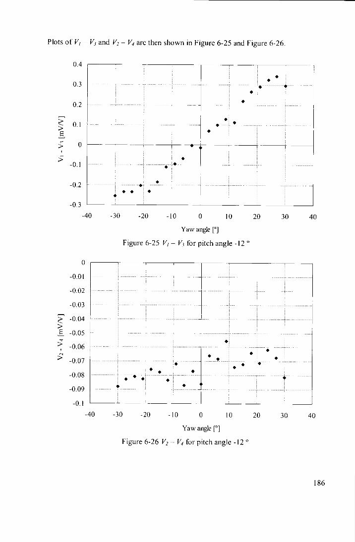
> E

> 0

^ -0.1

-0.2

-0.3

0

-0.01

-0.02

-0.03

-0.04 >

-0.05

> 1

-0.06 f N

> -0.07

-0.08

-0.09

-0.1

Plots of Vi - V} and V2 - V4 are then shown in Figure 6-25 and Figure 6-26

0.4

0.3

0.2

0.1

1 ^ •

•

• • i •

•

• t

-40 -30 -20 -10 0 10 20 30 40

Yaw angle [°]

Figure 6-25 V, - V} for pitch angle -12 "

-40 -30 -20 -10 0 10 20 30 40

Yaw angle \°]

Figure 6-26 V2 - V4 for pitch angle -12 °

186

There are no obvious problems with this data, and it can be seen that sensors 1 and 3 are

sensitive to yaw and sensors 2 and 4 are sensitive to pitch.

V,ou,i is plotted in Figure 6-27.

0.16

0.14

0.12

0.1

I 0.08

4 0.06 a c

> 0.04

0.02

0

-0.02

• i • -

• [

1 i •

• • ! •

-40 -30 -20 -10 0 10 20 30 40

Yaw angle ["]

Figure 6-27 V,n,ai for pitch angle -12°

This data shows no obvious major issues, although some variation, but note how close

the values at yaw angles of 6 and 9 ° are to zero.

Then plotting pitch and yaw coefficients in Figure 6-28 and Figure 6-29, it can be seen

the huge effect these very small values of have on the coefficients calculated. The

variation of yaw coefficient which should be seen with changing yaw angle is lost

because of variations in the total voltage when this is near zero.

187

c o

c o 'o e o CIS

45

40

35

30

25

20

S 15

10

5

0

-5

10

20

-20

-40

-60

-80

•100

• '• • • ^ • • • • • •

-40 -30 -20

* • • • • • ^ ! • • • • • • • •

-10 0 10 20 30 40

Yaw angle [°]

Figure 6-28 Pitch coefficient at pitch angle of -12°

-40 -30 -20 -10 0 10 20 30 40

Yaw angle ["]

Figure 6-29 Yaw coefficient at pitch angle of-12"

This problem could be partially alleviated by increasing the sensitivity of the sensors, so

that there is always more deflection of the cantilever sensors. Additionally, although the

188

probe is effective at measuring pitch and yaw, it does not have a good response to

changes in the velocity o f the flow. The response o f a probe sensor at varying velocities

with zero incidence is shown in Figure 6-30.

> • 4 - »

3

0.25

0.2

0.15 1

2 0.1 -O

g

0.05

10

* • j • ^

15 20

Velocity [nVs]

n —

25

• 0° incidence • 30° incidence

30

Figure 6-30 Response o f probe sensor to changes in velocity at two different incidence

angles

It can be seen that the probe shows very little response to the changes in velocity at zero

incidence, relative to the sensitivity to the incidence angle, and indeed that there is no

correlation between the increase in velocity and the voltage output.

However, when the same measurements are repeated with an incidence angle o f 30°, the

effects o f the changes in velocity are clearly visible. Consequently the sensor appears to

be able to measure changes in dynamic pressure but only at a significant incidence

angle. The lack o f sensitivity at zero incidence is probably due to the cancelling out of

the forces caused by the stagnation pressure at the centre o f the probe i.e. on the inside

of the sensor, and the force from the pressure on the outside o f the sensor caused by the

sensor being angled in towards the tip.

189

The overall response of the probe sensors is much lower than that predicted by the C F D

and F E modelling (Figure 6-15). The most likely reason for this is the presence of the

glue securing the sensors to the probe head. This glue can extend along the free under-

surface of the cantilever due to the assembly process. The glue would then increase the

stiffness of the cantilever sensor.

6.5 Revised probe design

6.5.1 Design

Due to these problems with the original design of probe, it was decided to alter the

design to try and improve the aspects which were causing problems. Although the probe

had been found to be relatively sensitive to pitch and yaw, the sensitivity to changes in

dynamic pressure at low incidence angles was a problem and also the sensitivity overall

would benefit by being increased.

In order to address these issues two changes were made to the design of the probe. The

problem of measuring velocity was tackled by changing the design of the probe head on

which the sensors were mounted. Instead of using the simpler angled design which

aimed to keep the probe tip diameter to a minimum, the pairs of sensors were mounted

parallel to each other instead of converging, The probe head, after narrowing down then

had sides parallel to each other for a length in order to allow this. This was expected to

increase the outward bend of the cantilevers when at zero incidence. However in order

to achieve this design by rapid prototyj^ing, the minimum achievable wall thickness was

0.5 mm with a 0.5 mm hole running through it. This meant that the tip diameter of the

probe would be increased to 1.5 mm from 0.5 mm. Increasing the diameter of the probe

tip was considered worthwhile in order to establish the viability of the new design, and

it would be possible to reduce the probe size again once the principle had been verified

by the use of an alternative rapid prototyi^ing system (possibly stereolithography),

capable of manufacturing objects with thinner walls and also achieving narrower holes.

190

The revised probe head is shown in Figure 6-31.

Figure 6-31 Revised probe head

To increase the sensitivity o f the sensors overall, the length o f the sensing cantilever

was increased from 1 mm to 1.5 mm. The new sensor design is shown in Figure 6-32.

The design is very similar to the previous one, with the exception o f the longer

cantilever, and an extended narrow section behind the strain gauge to allow the sensor

to be mounted on the new probe head design. In addition, the angle at which the sensor

narrowed from the contact pad region to the cantilever and also the length between these

two points was altered for the same reason. The fabrication process was identical to that

o f the initial design, with the different masks being used.

Contact pads

Strain gauge

Cantilever sensor Wheatstone bridge resistors

Figure 6-32 Diagram o f revised probe sensor

The construction of the probe was carried out using the same method as previously.

191

A close-up o f the tip o f the new probe is shown in Figure 6-33. The parallel nature o f

the cantilevers compared with the previous design where the cantilevers converged

towards the tip can clearly be seen in this picture.

Figure 6-33 Close-up o f tip o f revised probe design

6.5.2 Wind tunnel results

The response o f the sensor when parallel and perpendicular to the flow at varying yaw

angles at 20 m/s is shown in Figure 6-34.

> S

O

0.35

0.3

0.25

0.2

0.15

0.1

0.05

0

-0.05

-0.1

-0.15

• f • • •

• Sensor 1

• Sensor 2

Figure

-40 -30 -20 -10 0 10 20 30 40

Yaw [°]

6-34 Response o f revised sensors parallel and perpendicular to flow at varying

yaw angles

192

The response o f the sensor when perpendicular to the flow is very similar to that o f the

previous design o f probe, but gives a greater magnitude o f response as intended by

increasing the length o f the cantilever. However, the response of the sensor when

parallel to the flow is much greater than with the previous design. This indicates that the

probe is more sensitive to flows at low incidence angles, which was one o f the issues

being addressed by the new design o f probe. Sensor 2, which should be sensitive to

pitch, is seen to be independent o f yaw angle, indicating good decoupling o f pitch and

yaw sensitivities.

As seen with the previous design, the response o f the sensor was not the same for

negative and positive yaw angles. This is because at positive yaw angles, the flow onto

this sensor is occluded by the upstream sensor o f the pair.

The response o f the probe to changes in velocity was tested as wi th the previous design.

The results o f this testing are shown in Figure 6-35.

5 0.25 S-o

g 0.15

10

• 0° * 30°

15 25 30 20

Velocity [nVs]

Figure 6-35 Response o f revised probe sensor to changes in velocity at two different

incidence angles

193

It can be seen that the response of the sensor at zero incidence now has a response to

variation in the velocity compared with the previous design of probe which had no

response. This objective had therefore been achieved by altering the angle of the sensors

from converging to parallel. The response of the sensor when it is at an incidence angle

of 30° is seen to have a greater offset than that at 0°.

The decrease in the sensor output just above 20 m/s is most likely to be caused by the

flow over the cantilever stalling. The stalHng of the flow over the cantilever is shown in

Figure 6-36.

Airflow

Separated flow

Sensor

Sensor deflects to angle where flow behind cantilever separates, causing stall and loss of lift and subsequent decrease in deflection

Figure 6-36 Stalling of flow over cantilever sensor

To verify this, the response of the sensor at other incidence angles was also measured.

194

The results o f these experiments are shown in Figure 6-37.

>

3 O

g c/:i

0.6

0.5

0.4

0.3

0.2

0.1

0

-0.1

-0.2

-0.3

-0.4

. ; : \

i i

i i

** *

*

•-10"

1( 15 20

Vetocity [m/s]

25 30

Figure 6-37 Response o f revised probe sensor to changes in velocity at varying

incidence angles

It can be seen that as incidence angle increases the peak o f the response moves to the

left. This is as would be expected, since i f the initial incidence angle is greater, then a

lower velocity would be required to cause the cantilever to deflect to a position where

the flow stalls. At very high incidence angles the flow has stalled at a lower velocity

than the range shown here, hence why the effect was not seen for an incidence angle o f

30° in the previous figure.

At negative incidence angles the stall shifts to the right i.e. a higher velocity because the

initial incidence is less. At greater negative incidence angles, the flow onto the outside

o f the cantilever sensor causes a greater pressure than the pressure between the sensors,

and thus the cantilever bends inwards. In the range o f velocities shown here, a high

enough incidence angle is not reached to cause stall when the cantilevers are deflected

inwards.

195

The stall o f the sensors would not have been seen in the modelling as the deflection o f

the sensors was not introduced into the CFD work.

The standard deviation o f the data was considered for zero incidence. This is shown in

Figure 6-38.

0.35

^ 0.3 > ^ 0.25 3

p 0.2 O

i 0.15 <D

0.1

0.05

(I

— j

• Average

• Standard deviation

•

•

•

•

4 4

I

• •

•

•

0.00035

>

0.0002 ^

0.00015 I

0.0001 I

0.00005 ^

10 15 20

Velocity [m/s]

25 30

Figure 6-38 Standard deviation o f data at stall

The increase in the standard deviation after the f low has stalled backs up the theory that

this is what is taking place to cause the decrease in the sensor output.

An increased velocity would cause an increased curvature o f the cantilever; this would

increase the effective incidence angle, causing the flow to stall. The ' h f t ' on the

cantilever would then be decreased causing the curvature o f the cantilever and thus

effective incidence angle to decrease again, possibly causing the reattachment o f the

flow. This cycle would repeat so that although the peak response of the cantilever would

be increased, the mean value would decrease. This increase in the amplitude o f the

signal is reflected in the increasing standard deviation. Where the velocity is high

enough that the flow does not reattach there would still be increased fluctuations in the

position o f the cantilever due to the likelihood o f vortex shedding taking place.

196

Because o f the disruption at around 20 m/s caused by stalling at incidence angles close

to zero, the response o f the sensor to yaw (perpendicular and parallel to the flow) was

repeated at 27 m/s. The results are shown in Figure 6-39.

0.6

0.5

0.4

0.3

^ 0.2 > 6, 0.1

0

-0.1

-0.2

-0.3

-0.4

3

i

-J ( A

« • • •

<

i

• • • •

• • <

i

• • <

•

• !'

i ;

1 1 -

• • j •

! 1 1

• ^ •

• ; i i

• Sensor 1 • Sensor 2

-40 -30 -20 -10 0 10 20 30 40

Yaw [°]

Figure 6-39 Response o f revised sensors parallel and perpendicular to flow at varying

yaw angles (Velocity = 27 m/s)

At this velocity, the dips in sensor output at positive yaw angles are not seen, as the

range o f angles seen here are not close to stall at this velocity. The variation seen where

the sensor is parallel to the flow is much more defmed, with a clear increase in the

response o f the pitch sensors at high yaw angles, compared with the response at zero

incidence.

The apparently constant response of the sensor at positive incidence angles above 5° is

probably due to the upstream sensor partially occluding the flow onto the downstream

sensor. This should not be a problem for the calculation o f the yaw coefficient since at

corresponding negative yaw angles there is still a significant gradient at these values,

and thus the difference between the upstream and downstream sensors w i l l still vary

with yaw angle.

197

Using these results to calculate the coefficients gives the following results:

0.7

0.6

0.5

0.4

g o 0.3

IS

cj 0.2

0.1

0

-0.1 10 15 20

Yaw [°]

•

25

•

30

• Yaw 27 nVs

• Yaw 20 nys • Pitch 27 ffl/s • Pitch 20 m/s

35

Figure 6-40 Yaw coefficient for revised probe design

The yaw coefficient increases for increasing yaw angles as would be expected. The

coefficient for 20 m/s where the flow is close to the stall point shows a different

response to that at a higher velocity where the f low is more similar regardless of yaw

angle. Ideally the yaw coefficient would be the same, independent o f the velocity.

However a degree of Reynolds sensitivity means that the yaw coefficient o f probes is

often found to vary with velocity. The stall o f the flow over the cantilevers, in this case,

does however exacerbate the problem.

The pitch coefficient is close to zero for varying yaw angles.

198

The stagnation pressure coefficient is plotted in Figure 6-41.

50

£ c •J

d .o

on

0

-50 -

-100

-150 4

-200

-250

•

• 27 m/s • 20 m/s

0 10 25 30 35 15 20

Yaw [°]

Figure 6-41 Stagnation pressure coefficient for revised probe design

The stagnation pressure coefficient decreases with increasing yaw angle as would be

predicted. The coefficient is always negative as the probe pressure is referenced to total

pressure and therefore must always be less than zero. The difference between the

coefficients at different speeds when at higher yaw angles is due to Reynolds

sensitivity.

The angle for which the probe pressure stays close to total pressure indicates that the

probe is still seeing stagnation pressure at angles up to approximately 15°. Sheppard

[84] states that a hemispherical pitot-static tube would have an error o f less than 2.5%

for angles o f up to 30°. However, the presence o f the sensors and the blunt nature o f the

tip would reduce this angle.

199

The dynamic pressure coefficient is plotted in Figure 6-42.

0.0045

0.004

0.0035

0.003

0.0025

0.0015

0.0005

• 27 m/s • 20 m/s

0 10 25 30 35 15 20

Yaw [°]

Figure 6-42 Dynamic pressure coefficient for revised probe design

The dynamic pressure coefficient remains quite similar regardless o f Reynolds number

and deviates little with yaw angle, decreasing slightly as the yaw angle increases. The

major difference for the two velocities at zero yaw is due to the stalling o f the cantilever

that occurs at this angle at approximately 20 m/s. This does however cause a significant

problem with the use o f this coefficient for calculating the dynamic pressure from the

sensor outputs.

I f the total voltage output from all four sensors is plotted against dynamic pressure

(Figure 6-43) it can be seen that in the region between 240 and 420 Pa, as many as three

different dynamic pressures can be associated with the same voltage output. Because at

zero incidence all four sensors are affected by stall at the same velocity, it is impossible

to identify which o f the dynamic pressures is the correct one for a particular data set.

At increased incidence angles, although one o f the sensors may be close to stall the

opposing sensor w i l l not be in this region and therefore looking at both sensors

200

individually could be used to identify the true dynamic pressure. However at very small

incidence angles this does not provide a solution.

Unless a solution to this problem was found, probes would be out of range for a specific

range of velocities at small yaw angles. Changing the length of the sensors would alter

the region to be considered out of range.

1.4

1.2

i

> 0.8

1 0.6 >

0.4

0.2

0 - i -

0

Multiple Pdyn

for same Vtotai

• • Multiple Pdyn

for same Vtotai •

•

• i

100 400 500 200 300

Pdyn [Pa]

Figure 6-43 Dynamic pressure v. Total voltage output

Examples of the contour maps which would be generated when calibrating the probe are

shown in Figure 6-44 to Figure 6-47. These results are taken from the data obtained

from one sensor and generating the results from all four sensors, assuming that they

have the same response. This data is for tests carried out at 27 m/s.

In reality it is unlikely that the coefficients would be as symmetrical as those shown

here, since different sensors would be likely to have slightly varying responses. It would

therefore be necessary to calibrate individual probes separately.

201

-30 -20

o

-10 0 10 20 30 Yaw

Figure 6-44 Map of yaw coefficient

-20 -10 0 10 20 30 Yaw [°]

Figure 6-45 Map of pitch coefficient

202

30 [(mVA/)/Pa

Figure 6-46 Map o f dynamic pressure coefficient

o

1600

30 [ P a / ( m V ^ ]

Figure 6-47 Map of stagnation pressure coefficient

203

These plots show that the probe gives suitable resuhs in the regions between pure yaw

and pure pitch, which were looked at in more detail previously. The good decoupling of

pitch and yaw sensitivity is clear, and additionally it can be seen that the stagnation

pressure coefficient is relatively independent of yaw and pitch, except at extreme

angles.

6.6 Summary

A probe constructed from four cantilever sensors with a central pressure tapping was

used to measure pitch and yaw and also to give dynamic and stagnation pressure. This

design represented an entirely new method of constructing an airflow probe, utilising

MEMS technology to allow sensing elements smaller than could be achieved with

standard fabrication processes. This would lead to the construction of a probe with a

smaller tip diameter than is possible with conventional designs.

The probe design was modelled using CFD and FEA modelling which predicted that the

probe would be effective for measuring pitch and yaw coefficients at incidence angles

of up to ±40°.

Initial wind tunnel testing of the original probe design showed that the sensors were not

as sensitive as had been predicted by the modelling. In addition to this the probe had

very little sensitivity to changes in velocity at zero incidence.

To improve these difficulties, the probe was redesigned. The cantilever sensor's

positions were altered to be more parallel to the flow at zero incidence, which ensured

that the sensors bent outwards at zero incidence. When the sensors were orientated

inwards, for them to bend outwards required the pressure at the tip of the probe (close to

stagnation pressure) to be greater than the pressure on the outer surface of the

cantilever.

The new design of probe proved to have a much improved response to changes in

dynamic pressure at zero incidence. The response was very similar to that seen for a

sensor perpendicular to the flow when at incidence, but with a smaller magnitude of the

response, as would be expected. However for certain velocities at zero incidence, due to

204

the deflection of the sensor, the flow around the cantilever was seen to stall, causing an

irregularity in the response at a velocity of around 20 m/s. This stall point was also

observed at small positive and negative incidence angles, although the velocity at which

they occurred varied, due to the yaw angle causing a different effective incidence of the

flow onto the cantilever.

The stalling of the airflow meant that the probe would be ineffective at measuring

airflows at close to zero incidence angle to the flow, for a range of velocities around the

point where the flow stalled.

The overall sensitivity was also improved with the new design, due to increasing the

length of the cantilever by 50%. The sensitivity was still not as good as that which was

predicted by modelling however, and this decrease in the sensitivity was attributed to

the glue used to attach the sensors to the probe mounting extending along the under-

surface of the cantilever and making it stiffer than would be expected from the SU-8

polymer alone.

The method of using cantilever sensors to measure the velocity components when

constructed into a probe has been shown to be possible, allowing the creation of a probe

with a tip smaller than that which has been possible with previous methods. However

there are a number of improvements which could be made on the existing design. An

increase in the sensitivity of the sensors would improve the signal-to-noise ratio and

thus make the sensors more reliable. Improving the sensitivity would also allow the

cantilevers to be shortened, reducing the problem of stalling as this would then occur at

higher velocities. It would also be advantageous to increase the sensitivity sufficiently

that a stiffer material could be used in order to limit the deflection of the cantilevers

back into the airflow, as in the case of the shear stress sensor. However, the use of

silicon with a doped silicon piezoresistor would not be as applicable here, as the current

fabrication process requires some flexibility of the sensor for it to be mounted on the

probe head.

In addition the failure rate when assembling the probe is high and this should be

addressed. A number of problems can occur including shorting of the resistors when

205

attaching the wire, which could be solved by adding an additional layer of SU-8 over

the resistors which would not cover the contact pads. However this additional layer of

processing would be likely to increase the failure rate when fabricating the sensors. The

resistors are also prone to being damaged while being glued onto the mounting and this

aforementioned solution would also address this problem.

The assembly process is complex and prone to faults and an alternative assembly

method which would produce a more reliable result would be a significant

improvement. However because of the 3D nature of the probe, constructing the entire

probe by MEMS fabrication processes is not possible and therefore some degree of

assembly would always be required.

Once these fabrication problems were overcome it would be possible for a probe to be

constructed that would be ftilly fiinctional and, in addition, an alternative rapid

prototyper (possible SLA (Stereolithography Apparatus)) would allow a probe tip to be

created which was as small as 0.5 mm or less, which would be a significant

improvement on existing probes for measuring flow vectors.

206

Chapter 7

Conclusions

The aim of this thesis was to apply MEMS technology to the fabrication of airflow

sensors in order to improve the current available instrumentation. This required an

innovative approach to airflow measurement in order to fully utilise the potential of the

available techniques.

7.1 Fence-style shear stress sensor

Two different designs of shear stress sensors have been designed, fabricated and tested.

The first design was an adaptation of a surface fence design, which incorporated a strain

gauge into the fence structure in order to measure directly the pressure-induced

deflection of the fence. This structure was fabricated from the photo-definable polymer

SU-8 with a gold strain gauge incorporated within the fence to measure the deflection of

the fence caused by the airflow. This strain gauge was connected to a Wheatstone

bridge, which was within the body of the sensor to which the fence was attached.

207

CFD and FE modelling was carried out on the fence sensor to gain an understanding of

the response of the sensor to the airflow. Vortex shedding was found to take place at

higher Reynolds numbers.

The fence design of sensor was found, on wind tunnel testing, to be capable of

measuring wall shear stress. A response from the sensor of 0.18 mV was measured at a

shear stress of 0.35 Pa for an input voltage to the Wheatstone bridge of 1 V. However,

there were thermal effects caused by the resistive heating of the gold resistor and the

cooling that took place in the airflow. In addition to this the mounting of the fence

sensor required it to be embedded within the surface of the model that was being tested.

Also the fence protruded too high into the boundary layer, which would disturb the

airflow as it passed over the sensor.

7.2 Cantilever-style shear stress sensor

In order to address these issues, this initial sensor design was then built upon to create

an innovative new design of sensor, usmg an in-plane cantilever to measure the shear

stress by means of a built-in strain gauge to determine the pressure-induced deflection

of the cantilever.

The use of a cantilever allows greater sensitivity than the use of a fence, which is

effectively a beam with two fixed ends and the advantage of this in-plane cantilever

design over one mounted normal to the wall surface is that increasing the sensitivity by

increasing the length does not increase the frontal area of the cantilever seen by the

airflow. The velocity gradients in the axial direction are smallest and therefore the

spatial resolution of the sensor is least affected by the increase of the length of the

sensor in this direction. The width of the cantilever has no influence on the sensitivity of

the sensor and, although increasing the height of the cantilever above the wall would

increase the sensitivity, the sensor would then be higher in the boundary layer and thus

have a greater impact on the airflow passing over the sensor.

The pressure under the cantilever would be close to stagnation pressure, and a much

lower pressure would be seen above the cantilever. This would cause the cantilever to

deflect upwards and this deflection would be measured by a strain gauge incorporated

208

into the cantilever. The cantilever was fabricated from SU-8 as with the fence sensor,

but the strain gauge was fabricated from nichrome, which has a higher gauge factor than

gold, and also has a much lower thermal coefficient of resistivity which reduces the

thermal sensitivity of the sensor.

Modelling of the cantilever by CFD allowed a greater understanding of the airflow

passing over the sensor to be obtained. It was found that vortex shedding took place at

higher Reynolds numbers where the incidence angle of the cantilever was greater. The

airflow over the cantilever was found to stall as the incidence angle increased, but

although the lift consequently decreased, the drag continued to increase and therefore

the moment acting on the cantilever continued to increase after the flow stalled, albeit at

a slower rate. CFD modelling also predicted that the resistive heating of the strain gauge

would be minimal and have a negligible effect on the results from the cantilever. FE

modelling was also carried out to predict the voltage output response from the sensor,

which was found to be an order of magnitude greater than that of the fence sensor.

Mechanical testing was also carried out on the cantilever sensor in order to obtain an

accurate Young's modulus and gauge factor for the sensor, which were 1.45 GPa and

1.8 respectively.

Wind tunnel testing showed that the modelling of the sensor was quite accurate. The

shortest cantilever tested (2 mm long) was found to have a response of approximately

1 mV/V at 0.35 Pa. Longer cantilevers (3 and 4 mm long) were seen to bend back over

themselves at higher velocities. This would have a big impact on the airflow passing

over the sensor, and thus is an undesirable response indicating that the sensor is overly

sensitive for this application. Varying the width of the cantilever was not found to have

any effect on the response of the sensor.

There were found to be no thermal effects using this sensor as seen when using the

fence sensor. In addition the excitation voltage was found to have no effect on the

response of the sensor. Varying the axial position of the sensor showed that the sensor

can measure the shear stress where the boundary layer velocity profile varies.

209

The cantilever sensor was shown to effectively measure the wall shear stress for steady

state measurements in the laminar boundary layer. The device had a sensitivity an order

of magnitude better than that seen for the fence sensor.

The stated specification for the shear stress sensor designed in this work has largely

been achieved. A sensor capable of measuring low shear stresses has been

demonstrated. Although stresses up to 10 Pa have not been measured, the design of the

sensor is such that altering the geometry would allow stresses up o this magnitude to be

measured. The sensor is independent of ambient temperature as required and the design

of the sensor allows it to be surface-mounted on any existing model. The requirement

for high frequency measurements did not come within the scope of this work.

7.3 Probe for freestream flow vector measurement

The cantilever shear stress sensor was adapted into a probe for measuring freestream

velocity components and would also allow the measurement of stagnation and dynamic

pressures.

Four sensors were incorporated into one probe head in order to allow three-dimensional

measurement. These sensors were mounted in two pairs normal to each other. One pair

of sensors was largely sensitive to yaw, and the other pair was sensitive to pitch. The

probe head on which the sensors were mounted had a hole running through it allowing

the pressure at the centre of the probe to be measured for the calculation of the

stagnation pressure. The movement of all four sensors together could measure the

dynamic pressure.

Modelling of the probe was carried out using CFD in 3D. This predicted pressure

differences across the cantilever sensors which, when combined with finite element

modelling predictions gave expected output values similar to those seen in the

cantilever wall shear stress sensor. This was because, despite the shorter length of the

cantilever, the velocity seen by the cantilever was significantly greater as the sensor was

not in the boundary layer where the velocities were much lower.

210

Wind tunnel testing of the probe showed significantly lower sensitivity than predicted,

which was attributed at least in part to the fabrication method causing glue to reduce the

deflection of the cantilever. However in addition to this the probe was found to have a

negligible response to varying velocities at zero incidence angles.

To address this issue the probe was redesigned, and the new design was found to

partially deal with this problem. The sensor was sensitive to changes in velocity at zero

incidence. However, the flow over the sensor stalled at a velocity of just over 20 m/s at

zero incidence, meaning that a probe of this design would be out of range for very small

incidence angles in the region around this velocity. The sensitivity of the device was

also improved with this new design. A single sensor at +30° incidence at 20 m/s gives a

response of 0.3 mV/V, with a response of -0.1 mV/V at -30° incidence at 20 m/s.

Four sensors in this arrangement have been shown to allow the measurement of pitch

and yaw, as well as the stagnation and dynamic pressures.

The objectives for this work have been partially achieved. A probe with the capability

of measuring 3D flow vectors in the velocity range specified has been demonstrated.

The stated yaw and pitch range is within the capability of the probe. However it was not

found possible to minimise the probe tip beyond what was already possible with a

conventional five-hole probe. However there is the potential to reduce the tip diameter

with ftirther work. The development of the probe for high frequency measurements was

not completed within the scope of this work.

7.4 Further work

7.4.1 Wall shear stress sensors

Since the cantilever design of wall shear stress sensor supersedes the fence design, the

focus here on fiiture work will be directed toward the cantilever design.

The current materials used for the construction of the sensors allow a good sensitivity

by means of a low Young's modulus that compensates for the fact that the gauge factor

of a metal strain gauge is relatively low. However this means that the deflection of the

21

sensor is relatively large, which has a detrimental effect on the airflow. A method of

overcoming this problem would be to achieve the sensitivity by means of a high gauge

factor, with a relatively higher Young's modulus. This could be accomplished by

fabricating the sensor from silicon with a doped silicon strain gauge.

A collateral advantage of this alteration would be to increase the resonant frequency of

the cantilever, which would be an advantage in the measurement of turbulent, unsteady

flows.

The current set-up for shear stress measurement is only suitable for steady state

measurements as the signal-to-noise ratio is sufficiently low as to require a filter to be

used to reduce the noise level. The use of a lock-in amplifier might allow this problem

to be addressed in such a way that the frequency response of the sensor would be

unaffected, allowing time-varying measurements to be taken. However lock-in

amplifiers are normally used for ac voltage measurements.

7.4.2 Probe for freestream flow vector measurement

The assembly of the probe offers several opportunities for improvement. If, as

postulated, the decrease in sensitivity compared with that which was predicted was due

to the glue applied during the assembly process, then modifying this fabrication process

should improve the sensitivity of the sensors. Also, the difficulty of attaching wires to

such small contact pads could also be improved. There is the possibility of wire bonding

for making the connections to the sensors, which would allow the size of the probe to be

kept small close to the probe tip; however the difficulty of attaching wires, of

dimensions large enough to handle, to the fine wires used for wire bonding would

remain. Once this assembly problem had been addressed, a probe with four frilly

functional sensors could be created, which could then be tested in a real application.

The deflection of the cantilever sensor should be minimised as was the case with the

wall shear stress sensor, in order to keep the probe tip size as small as possible during

operation. However the use of silicon as suggested for that application would not be

suitable here since the assembly process relies on the flexibility of the SU-8 to allow the

sensors to be mounted on the probe.

212

References

1 Fernholz HH, Janke G, Schober M, Wagner PM and Warnack D New developments

and applications of skin-fi-iction measuring techniques Meas. Sci. Technol. 7 1396-1409

(1996)

2 Sheplak M, Cattafesta L and Nishida T MEMS shear stress sensors: promise and

progress 24''' AlAA Aerodynamic Measuvemenl Technolog}> and Ground Testing

Conference (2004)

3 Naughton JW and Sheplak M Modem developments in shear-stress measurement

Progress in Aerospace Sciences 3 8 515-570 (2002)

4 Squire LC The motion of a thin oil sheet under the boundary layer on a body J. Fluid

Mech. 11 161-179 (1961)

5 Tanner LH and Blows LG A study of the motion of oil films on surfaces in air flow,

with application to the measurement of skin friction J/'/7>'5 £ 9 ( 3 ) 194-202 (1976)

6 Murphy JD and Westphal RV The laser interferometer skin-friction meter: a

numerical and experimental study J £ 19 744-51 (1986)

7 Pradeep A M and Sullerey RK Application of shear stress sensitive liquid crystals in

flow visualisation and skin friction estimation Optical Diagnostics in Engineering 7 t-9

(2004)

8 Buttsworth DR, Elston SJ and Jones TV Directional sensitivity of skin friction

measurements using nematic liquid crystal Meas. Sci. Techno/. 9 1856-1865 (1998)

9 Fujisawa N, Aoyama A and Kosaka S Measurement of shear-stress distribution over a

surface by liquid-crystal coating Meo^. Sci. Techno/. 14 1655-1661 (2003)

10 Padmanabhan A, Goldberg HD, Breuer KS and Schmidt MA A silicon micro-

machined floating-element shear-stress sensor with optical position sensing by

photodiodes Proc. of Transducers (Stockholm, Sweden) p 436-439 (1995)

11 Horowitz S, Chen T, Chandrasekaran V, Tedjojuwono K, Nishida T, Cattafesta L

and Sheplak M A micromachined geometric moire inteferometric floating-element

213

shear stress sensor A I A A Paper 2004-1042 42"'' Aerospace Sciences Meeting and

Exhibit (Reno, N V ) (2004)

12 Zhe J, Farmer KR and Modi V A MEMS device for measurement o f skin friction

with capacitive sensing Proc. of IEEE MEMS 2001 (Berkeley, CA) p 4-7 (2001)

13 Desai A V and Haque M A Design and fabrication o f a direction sensitive MEMS

shear stress sensor with high spatial and temporal resolution ./. Micromech. Microeng

14 1718-1725 (2004)

14 Alvin Barlian A, Park S-J, Mukundan V and Pruitt B L Design and characterization

o f microfabricated piezoresistive floating element-based shear stress sensors Sensors

and Actuators A 134 77-87 (2006)

15 Bruun H H Hot wire anemometry: Principles and signal analysis Oxford University

Press 237-253 (1995)

16 Sheplak M , Chandrasekaran V, Cain A, Nishida T and Cattafesta L N

Characterization o f a silicon-micomachined thermal shear-stress sensor AIAA Journal

40 6 (2002)

17 Huang JB, Jiang FK, Tai Y C and Ho CM A micro-electro-mechanical-system-based

thermal shear-stress sensor with self-frequency compensation Meas. Sci. Technol. 10

687-696 (1999)

18 Elvery DG and Bremhorst K Directional sensitivity o f wall mounted hot-film gauges

Meas. Sci. Techno/. 7 1410-1417(1996)

19 Dengel P and Fernholz H H An experimental investigation o f an incompressible

turbulent boundary layer in the vicinity of separation J. Fluid Mech. 212 615-636

(1990)

20 Chen J, Zou J and L iu C A surface micromachined, out-of-plane anemometer Proc.

of IEEE MEMS 2002 (Las Vegas, N V ) p 332-335 (2002)

21 Liu C, Huang J-B, Zhu Z, Jiang F, Tung S, Tai Y-C and Ho C-M A micromachined

flow shear-stress sensor based on thermal transfer principles ./. of Microelectromech.

8 90-99(1999)

214

22 Tung S, Rokadia H and L i WJ A micro shear stress sensor based on laterally aligned

carbon nanotubes Sensors and Actuators A 133 431 -438 (2007)

23 Fourgette D, Modarress D, Taugwalder F, Wilson D, Koochesfahani M and

Gharib M Miniature and MOEMS flow sensors AIAA Paper 2001-2982 (2001)

24 Vagt JD and Fernholz H Use o f surface fences to measure wall shear stress in tliree-

dimensional boundary \ayers Aeronautical Quarterly 24 87-91 (1973)

25 Papen T, Steffes H , Ngo HD and Obermeier E A micro surface fence probe for the

application in flow reversal areas Sensors and Actuators A 97-98 264-270 (2002)

26 Papen T, Buder U , Ngo HD and Obermeier E A second generation MEMS surface

fence sensor for high resolution wall shear stress measurement Sensors and Actuators A

113 151-155 (2004)

27 Schober M , Obermeier E, Pirskawetz S and Fernholz H H A MEMS skin-fiiction

sensor for time resolved measurements in separated flows Exp. in Fluids 36 593-99

(2004)

28 Chen J, Engel J and Liu C Development o f polymer-based artificial haircell using

surface micromachining and 3D assembly Transducers 2003 (Boston) (2003)

29 Briicker C, Spatz J and Schi-oder W Wall shear stress imaging using micro-structured

surfaces with flexible micro-pillars Exp. in Fluids 39 464-474 2005

30 GroPe S and Schroder W Mean wall-shear stress measurements using the micro-

pillar shear-stress sensor MPS^ Meas. Sci. Technol. 19 015403 (2008)

31 Patel VC Calibration o f the Preston tube and limitations on its use in pressure

gradients J. Fluid Mech. 23185-208 (1965)

32 Adrain RJ Twenty years o f particle image velocimetry Exp. in Fluids 39 159-169

(2005)

33 Adrian RJ Scattering particle characteristics and their effect on pulsed laser

measurements o f fluid flow: speckle velocimetry vs particle image velocimetry Appl.

Opt. 23 1690-1691 (1984)

215

34 Pickering CJD and Halliwell N A Laser speckle photography and particle image

velocimetry: photographic f i lm noise Appl. Opi. 23 2961-2969

35 Maas HG, Giiien A and Papantoniou D Particle tracking velocimetry in three-

dimensional flows Part 1. Photogrammetric determination o f particle coordinates Exp.

in Fluids 15 133-146

36 Pereira F and Gharib M Defocusing digital particle image velocimetry and the three-

dimensional characterization o f two-phase flows Meas. Sci. Technol. 13 683-694 (2002)

37 Barnhart DH, Adrian RJ and Papen GC Phase-conjugate holographic system for

high-resolution particle-image v e l o c i m e t r y O p t . 33 7159-7170 (1994)

38 Royer H Holography and particle image velocimetry Meas. Sci. Technol. 8 1562-

1572(1997)

39 Santiago JG, Wereley ST, Meinhart CD, Beebe DJ and Adrian RJ A particle image

velocimetry system for microfluidics Exp. in Fluids 25 316-316(1998)

40 Penner SS and Jerskey T Use o f lasers for local measurement o f velocity

components, species densities and temperatures Annu. Rev. Fluid Mech. 5 9-30 (1973)

41 Wang CP and Schnyder D Laser Doppler Velocimetry: Experimental Study Appl.

Opt. 13 98-103 (1974)

42 Czarske JW Laser Doppler velocimetry using powerful solid-state light sources

Meas. Sci. Technol. 17R71-R91 (2006)

43 Kupferschmied P, Koppel P, Gizzi W, Roduner C and Gyarmathy G Time-resolved

flow measurements with fast-response aerodynamic probes in turbomachines Meas. Sci.

Technol. 11 1036-1054(2000)

44 Sieverding CH, Arts T, Denos R and Brouckaert J-F Measurement techniques for

unsteady flows in turbomachines Exp. in Fluids 28 285-321 (2000)

45 Ligrani PM, Singer BA and Baun LR Miniature five-hole pressure probe for

measurement o f three mean velocity components in low-speed flows J. Phys. E: Sci.

Instnm. 22 868-876(1989)

216

46 Lenherr C, Kalfas A I , and Abhari RS A flow adaptive aerodynamic probe concept

for turbomachinery Meas. Sci. Techno/. 18 2599-2608 (2007)

47 Ainsworth RW, Miller RJ, Moss RW and Thorpe SJ Unsteady pressure measurement

Meas. Sci. Techno!. 11 1055-1076(2000)

48 Babinsky H, Kusche! U, Hodson HP, Moore DF and Wellard ME The aerodynamic

design and use o f multi-sensor pressure probes for MEMS applications 15''' Bi-annual

Symposium on Measuring Techniques in Turbomachineiy (Florence, Italy) (2000)

49 Lemonis G Three-dimensional measurement o f velocity, velocity gradients and

related properties in turbulent flows Aerospace Science and Technology 7 453-461

(1997)

50 Sherif SA and Fletcher R l l A normal sensor hot-wire/film probe method for the

analysis o f three-dimensional flows Flow Meas. Instrum. 5 150-154 (1994)

51 Samet M and Einav S A hot-wire technique for simultaneous measurement o f

instantaneous velocities in 3D flows / Phys. E: Sci. Instrum 20 683-690 (1987)

52 Tsinober A, Kit E and Dracos T Experimental investigation o f the field o f velocity

gradients in turbulent flows J. Fluid Mech. 242 169-192 (1992)

53 Van Di jk A and Nieuwstadt FTM The calibration o f (multi-) hot-wire probes 2.

Velocity-calibration Exp. in Fluids 36 550-564 (2004)

54 Shaw JM, Gelorme JD, LaBianca NC, Conley WE, Holmes SJ Negative photoresists

for optical l i thography/5M J. Res. Develop. 41(1/2) (1997)

55 Chuang Y-J, Tseng F-G, Lin W - K Reduction o f diffraction effect o f U V exposure on

SU-8 negative thick photoresist by air gap elimination Microsyst. Technol. 8 308-313

(2002)

56 Dai W, Lian K, Wang W A quantitative study on the adhesion property o f cured SU-

8 on various metallic surfaces Microsyst. Technol. 11 526-534 (2005)

57 Flint and Partners Flint Wind tunnel TE44 Manual

58 Kreyszig E Advanced Engineering Mathematics S"' ed. John Wiley & Sons Inc.

p . l 110 (1999)

217

59 Massey B Mechanics o f Fluids 7"' ed. Stanley Thornes (Publishers) Ltd 369-375

(1998)

60 Tannehill JC, Anderson DA and Pletcher RH Computational Fluid Mechanics and

Heat Transfer 2'"' ed. Taylor and Francis (1997)

61 Benham PP, Crawford RJ and Armstrong CG Mechanics o f Engineering Materials

2"" ed. Longman p.206 (1996)

62 Strand7 Finite Element Analysis System Documentation

63 Thaysen J, Yalcinkaya AD, Vettiger P and Menon A Polymer-based stress sensor

with integrated readout / Phys. D: Appl. Phys. 25 2698-2703 (2002)

64 Massey B Mechanics o f Fluids 7' ed. Stanley Thomcs (Publishers) Ltd 326 (1998)

65 Fox RW, McDonald AT, Pritchard PJ Introduction to Fluid Mechanics 6'' ed. John

Wiley and Sons 427 (2004)

66 Johnson SA, Thompson MC, Hourigan K Flow past elliptical cylinders at low

Reynolds numbers 14''' Australasian Fluid Mechanics Conference (2001)

67 Dellmann L, Roth S, Beuret C, Racine G, Lorenz H , Despont M , Renaud P, Vettiger

P and de Rooij N Fabrication process o f high aspect ratio elastic and SU-8 structures for

piezoelectric motor application Sensors and Actuators A 70 42-47 (1998)

68 Lorenz H , Despont M , Fahmi N , LaBianca N , Renaud P and Vettiger P SU-8: a low-

cost negative resist for MEMS J. Micromech. Microeng. 1 121-124(1997)

69 Chang S, Warren J and Chiang F Mechanical testing of EPON SU-8 with SIEM

Proc. Of Microscale Systems: Mechanics and Measurement Symposium Orlando, FL

46-49 (2000)

70 Wen Y - H , Yang GY, Bailey VJ, Lin G, Tang WC and Keyak JH Mechanically

robust micro-fabricated strain gauges for use on bones Proc. of 3'^ Annual IEEE EMBS

Conf. on Microtechnologies in Medicine and Biolog)> Oahu, Hawaii (2005)

71 Khoo HS, Liu K and Tseng F Mechanical strength and interfacial failure analysis o f

cantilevered SU-8 micropostsJ. Micromech. Microeng. 13 822-831 (2003)

218

72 Engel J, Chen J and Liu C Strain sensitivity enhancement o f thin metal f i lm strain

gauges on polymer microscale structures Appl. Phys. Lett. 89 221907 (2006)

73 Thomson WT Theory o f Vibration with Applications 4"' ed. Chapman and Hall

(1993)

74 Sameoto D, Tsang S-H, Foulds IG, Lee S-W, Parameswaran M Control o f the out-

of-plane curvature in SU-8 compliant microstructures by exposure dose and baking

times 7. Micromech. Microeng. 17 1093-1098 (2007)

75 Ericson F, Greek S, Soderkvist J and Schweitz J High sensitivity surface

micromachined structures for internal stress and stress gradient evaluation J.

Micromech. Microeng. 7 30-36 (1997)

76 Bachmann D, Schoberle B, Kuhns S, Leiner Y and Hierold C Fabrication and

characterization o f folded SU-8 suspensions for MEMS applications Sensors and

Actuators A 130-131 379-386(2006)

77 Rolke J Nichrome thin f i lm technology and its application Electrocomponent Science

and Technology 951-57(1981)

78 Sato Y, Watanabe M and Sato S Electrical properties o f Ni-Cr-N thin films deposited

by multitarget reactive sputtering J/?/?./. Appl. Phys. 40 5091-5094 (2001)

79 Kazi I , Wild P, Moore T and Sayer M The electromechanical behaviour o f nichrome

(80/20 wx.%) film Thin Solid Films 433 337-343 (2003)

80 Lee B-J, Lee D-C Electrical properties o f sputtered Ni-Cr-Al-Cu thin film resistors

with N i and Cr contents Journal of the Korean Physical Society 40 339-343 (2002)

81 Lee B-J, Lee B-H and Lee D-C Quaternary alloy films for thin film resistors Jpn J.

Appl. Phys. 42 1405-1409 (2003)

82 Pohlhausen E Der Warmeaustausch zwischen festen Korpern und Fliissigkeiten mit

kleiner Reibung und kleiner Warmeleitung. Z. Angew. Math. Mech. 1, 115-121 (1921)

83 Durham Software for Wind-Tunnels, User manual

84 Sheppard PA Anemometry: A critical and historical survey Proc. Phys. Soc. 53 361-

390 (1941)

219

••ay,--./