Durable–Goods Monopoly with Varying Cohorts

Simon Board∗

This Version: January 29, 2005

First Version: June 2003

Abstract

This paper solves for the profit maximising strategy of a durable–goods monopolist whenincoming demand varies over time. Each period an additional demand curve enters themarket; these consumers can then choose whether and when to purchase. The potential fordelay creates an asymmetry in the optimal price path which exhibits fast increases and slowdeclines. This asymmetry also pushes the price level above that charged by a firm facingthe average level of demand. Applications of this framework include deterministic demandcycles, one–off shocks and IID demand draws. The optimal policy can be implemented bya best–price provision and outperforms renting.

1 Introduction

Each September thousands of students return to universities and colleges across Canada. Cana-dian Tire, a large retailer, responds to this influx of new consumers by holding a back–to–schoolsale, reducing their price on furniture, stationary and kitchen utensils. While the price reduc-tion helps increase profits from the student community, it also causes customers who wouldhave bought in July and August to delay their purchases. This paper analyses this tradeoff,solving for the optimal pricing strategy of a durable–goods monopolist when incoming demandvaries over time.

Consider a monopolist selling a durable good, defined broadly to be any product whereagents can choose both whether and when to purchase. Each period the market is kept alive bythe entry of new consumers. These new consumers are associated with a demand curve which is

∗Department of Economics, University of Toronto. http://www.economics.utoronto.ca/board. I am indebtedto my advisor, Jeremy Bulow. I also received many helpful comments from David Ahn, David Baron, WillieFuchs, Ilan Kremer, John McMillan, Robert McMillan, Barry Nalebuff, Richard Saouma, Ilya Segal, AndySkrzypacz and Jeff Zwiebel. I have benefited from seminars at Cambridge, Essex, LSE, Northwestern, NYU,Oxford, Penn, Rochester, UC San Diego, Stanford, UT Austin, Toronto and Yale. An earlier version of thispaper went under the rather nebulous title of “Dynamic Monopoly”.

1

allowed to change over time. The firm’s problem is to choose a sequence of prices to maximisetheir profits subject to consumers optimally choosing their purchase time.

Each consumer’s purchase decision can be analysed as an optimal stopping problem. Usingthis formulation the paper characterises the consumers’ purchasing rule by a sequence of cutoffs:at any time t a consumer purchases if their valuation lies above the time–t cutoff. Mechanismdesign can then be utilised to describe the firm’s profit as a function of these cutoffs.

Under a monotonicity condition the profit–maximising cutoffs are characterised by a myopicalgorithm, where the allocation at time t only depends upon the consumers who have enteredthe market up to time t. Consumers are forward looking and prices depend upon the sequence offuture demand; the optimal allocation, however, only depends upon past demand. The optimalprices can then be derived from the consumers’ optimal purchase problem.

The optimal myopic algorithm has an intuitive interpretation. The new demand curve inany period t can be associated with a marginal revenue curve, where marginal revenue is withrespect to price, not quantity. In the first round the firm sells the good to agents with positivemarginal revenue (net of costs). In each period thereafter, the firm adds the marginal revenueof the old consumers who have yet to buy to that of the new agents, forming a cumulativemarginal revenue function. The firm then sells the good to agents with positive cumulativemarginal revenue.

Consumers’ ability to delay induces an asymmetry in the optimal price path. When demandgrows stronger over time, in that valuations tend to rise, the firm will want to increase theirprice. Agents then have no incentive to delay and the firm can discriminate between the differentgenerations, charging the monopoly price against the incoming generation: the myopic price.

When demand weakens over time, in that valuations tend to fall, the firm will want todecrease their price over time. Charging the myopic price, however, will now lead to fallingprices, causing some customers to delay their purchases. Anticipating this delay, the firm slowsthe rate at which prices fall. This decline in price is reduced so much that prices always stayabove that chosen by a firm who pools all generations together and prices against the averagelevel of demand: the average–demand price.

The contrast between increases and decreases in demand is stark. If there is a permanentand unanticipated increase in demand the price quickly jumps up to the new higher monopolyprice. However if demand falls the price will jump down a little and slowly fall towards thelower monopoly price over time.

This asymmetry between demand increases and decreases crucially affects the firm’s optimalpricing policy. When demand follows stationary cycles, it leads to sharp price increases andgentle declines. This is shown in Figure 1, where the lower panel describes which generationspurchase in which periods.

During the first quarter of the cycle, as demand rises from its average level to the peak of

2

20 40 60 80 100 1200

20

40

60

80

100

120

Time

Act

ive

gene

ratio

ns

20 40 60 80 100 12010

11

12

13

14

15

16

Pric

es

Optimal Cutoffs

Optimal Prices

Myopic Price

Average Demand Price

Figure 1: Price Cycles

the boom, the price rises quickly. For the other three–quarters of the cycle, as demand falls andthen returns to its average position, the price slowly falls. These price cycles are stationary,showing no decline in amplitude no matter how long the market has existed. The price is alsominimized not in the period of lowest demand, but in the last period of the slump, just beforedemand returns to its average position. The asymmetry between increases and decreases indemand also raises the price level: price always exceeds the average–demand price. This meansintroducing variation in demand leads to an increase in all prices. In other words, when thefirm has more information about demand cycles all consumers are made worse off and socialwelfare is reduced.

The basic model makes two assumptions of note.First, there is no resale. There are many goods where this is the right assumption: one–time

3

experiences, (e.g. a trip to Disneyland), intermediate products (e.g. aluminium), regulated mar-kets (e.g. plutonium), potential lemons (e.g. computers), goods with high transactions costs(e.g. fridges) or those with emotional attachment (e.g. diamonds). However such an assumptionis not innocuous. With perfect resale price variations decrease in amplitude as the market getsolder; without resale the market fluctuations never abate. With resale price responds symmetri-cally to changes in demand; without resale price movements are highly asymmetric. Introducingresale has no effect on allocations if and only if new demand falls over time; otherwise the pres-ence of resale lowers the monopolist’s profits. Since renting is identical to commitment pricingwith resale, renting attains maximal profits if and only if demand is declining.

Second, it is assumed that the monopolist can perfectly commit to a sequence of prices.With homogenous demand and no commitment there are many equilibria ranging from thethose that are very bad for the firm to others which are close to the full–commitment outcome(Sobel (1991)). This paper should thus be viewed as establishing the best possible outcome forthe firm. This seems particularly reasonable if the firm is concerned about its reputation acrossseveral durable–goods markets. In addition, there are contractual solutions to the commitmentproblem. We extend the result of Butz (1990) by showing if the firm can use a best–priceprovision they can implement the optimal scheme without requiring the pre–commitment.

The starting point for this paper are the models of Stokey (1979) and Conlisk, Gerstner,and Sobel (1984), as examined in Section 3.2. Other authors introduce dynamics into durablegoods models in different ways. Conlisk (1984), Laffont and Tirole (1996), Biehl (2001), andBoard (2004) have stochastic valuations. Cost variations have been analysed by Stokey (1979),and Levhari and Pindyck (1981). When consumers and the firm have different discount ratesthe optimal price may fall over time as examined by Sobel and Takahashi (1983), Landsbergerand Meilijson (1985), and Wang (2001). Rust (1985, 1986), Waldman (1996) and Hendel andLizzeri (1999) allow the good to depreciate and for consumers to scrap their the product.

The paper is organised as follows: Section 2 contains a description of the model and aderivation of the firm’s problem. Section 3 derives optimal control problem which is solved inSection 4. Section 5 discusses applications including monotone demand paths, one–off shocks,demand cycles and IID demand. Section 6 examines the effect of information structures, dis-count rates and best–price schemes. Section 7 analyses resale and renting, while Section 8concludes. Omitted proofs are contained in the Appendix.

2 Model

Time is discrete, t ∈ 1, . . . , T, where we allow T = ∞. Demand and the discount rate areallowed to be uncertain, depending on the state of the world ω ∈ Ω. The information possessedby consumer and the firm is described by a filtered space (Ω,F , Ft, Q), where F are the

4

measurable sets, Ft is the information partition at time t, which grows finer over time, andQ is the probability measure. The common discount rate, δt ∈ (δ, δ) ⊂ (0, 1), is Ft–measurable,i.e. ω : δt ≤ x ∈ Ft for x ∈ (0, 1). This means that at time t all agents know δt. Let thediscounting up to time t be ∆t =

∏ts=1 δs, where ∆∞=0.

A consumer with valuation θ ∈ [θ, θ] who purchases at time t ∈ 1, . . . , T,∞ at price pt

obtains utility(θ − pt)∆t

A consumer always has the option not to purchase, in which case they have zero utility and aresaid to buy at time t = ∞.

Each period consumers of measure ft(θ) enter the market. Let Ft(θ) be the distributionfunction, where Ft(θ) is the total number of agents (and not necessarily equal to one), anddenote the survival function by F t(θ) := Ft(θ)− Ft(θ). The time–t demand function, ft(θ), isFt–adapted, so while agents may not know future demand, they do know current demand. Thisavoids issues to demand experimentation and is trivially satisfied if demand is deterministic.

Consider a consumer of type (θ, t) with valuation θ who enters in period t. Given a sequenceof Ft–adapted prices, pt, they have the problem of choosing a purchasing time τ(θ, t) ≥ t tomaximise expected utility,

ut(θ) = E [(θ − pτ )∆τ ] (2.1)

where “E” is the expectation over Ω. The purchasing time is a random variable taking valuesin t, . . . , T,∞, where the decision to buy at time t can only depend on information availableat time t, i.e. ω : τ ≤ t ∈ Ft (∀t). Let τ∗(θ, t) be the earliest solution to this problem whichexists by Lemma 1 in Section 3.3.

The firm’s problem is to choose Ft–adapted prices pt to maximise profit. Assumingmarginal cost is constant, it can be normalised to zero, yielding expected profit,

Π = E[

T∑

t=1

∫ θ

θ∆τ(θ,t)pτ∗(θ,t) dFt

](2.2)

where τ∗(θ, t) maximises the consumer’s utility (2.1). In Appendix A.2 it is argued that therestriction to a price mechanism is without loss.

3 Solution Technique

3.1 Firm’s Problem

Since the purchase time is chosen optimally, we can apply the envelope theorem to the con-sumer’s utility maximisation problem (2.1). The space of stopping times is complex so we will

5

use the generalised envelope theorem of Milgrom and Segal (2002).1 This yields utility,

ut(θ) = E[∫ θ

θ∆τ∗(x,t) dx + u(θ, t)

](3.1)

Since the seller will always choose prices pt ≥ θ (∀t) it will be the case that u(θ, t) = 0 (∀t).Integrating by parts, consumer surplus from generation t is

∫ θ

θut(θ) dFt = E

[∫ θ

θ∆τ∗(θ,t)F t(θ) dθ

∣∣∣∣ Ft

](3.2)

Expected welfare from generation t is defined by

Wt := E[∫ θ

θ∆τ∗(θ,t)θ dFt

](3.3)

with total welfare W =∑

t Wt. Since costs are zero, the welfare maximising pricing schemeis to set all prices equal to zero. Expected profit equals welfare (3.3) minus consumer surplus(3.2),

Π = E[

T∑

t=1

∫ θ

θ

[∆τ∗(θ,t)θ − ut(θ)

]dFt

]

= E[

T∑

t=1

∫ θ

θ∆τ∗(θ,t)mt(θ) dθ

](3.4)

where mt(θ) := θft(θ)− F t(θ) is marginal revenue with respect to price.2

Profit is thus the discounted sum of marginal revenues. Notice how the marginal revenuegained from agent (θ, t) is the same no matter when they choose to buy. That is, an agent’smarginal revenue is determined when they are born, and sticks to them forever.

The firm’s problem is to choose prices pt to maximise profit (3.4) subject to consumerschoosing their purchasing time τ∗(θ, t) to maximise utility (2.1).

3.2 Special Cases

We now consider three special cases that will be useful benchmarks for what follows. Example1 comes from Stokey (1979), where there is a single demand curve of consumers and entry

1This theorem requires that the set of optimal purchasing times is nonempty, which is true by Lemma 1 inSection 3.3.

2It is more common to use marginal revenue with respect to quantity, MRt(θ) := mt(θ)/ft(θ). However,since we will be adding demand across generations, summing demand curves horizontally, it is easier to workwith marginal revenue with respect to price. In any case, both mt(θ) and MRt(θ) have the same roots, and arethus interchangeable in pricing formulae.

6

never occurs. Example 2 supposes the monopolist can set a different price schedule for eachgeneration. Example 3 is the homogenous entry model of Conlisk, Gerstner, and Sobel (1984).

Example 1 (Single Generation). If ft(θ) = 0 for t ≥ 2 the profit (3.4) reduces to

Π =∫ θ

θ∆τ∗(θ,t)m1(θ) dθ (3.5)

To maximise (3.5) the firm would like to set purchasing times as follows:

τ∗(θ, 1) = 1 if m1(θ) ≥ 0

τ∗(θ, 1) = ∞ if m1(θ) < 0

That is, the firm would like positive marginal revenue customers to purchase immediately, andthe rest to never buy. If m1(θ) is increasing this optimal policy can be implemented by setting

p1 = m−11 (0)

pt ≥ m−11 (0) if t ≥ 2

Since the price is increasing, consumers buy in period 1 or never buy at all. A consumer thenbuys in period 1 if and only if θ ≥ m−1

1 (0), which is the same as m1(θ) ≥ 0. 4

Example 2 (Discrimination between Generations). Next suppose the firm could tell thedifferent cohorts apart and set a price ps

t for generation s in time t. They would then implementStokey’s solution for each cohort. That is,

pst = m−1

s (0) if t = s

pst ≥ m−1

s (0) if t ≥ s + 1

Hence if the myopic monopoly price grows over time, m−1t (0) ≥ m−1

t−1(0), the seller can simplycharge the myopic price, p∗t = m−1

t (0), and need not discriminate. Example 3 amounts to aspecial case of this observation. 4

Example 3 (Homogenous Demand). Finally suppose demand is identical in each period,ft(θ) = f0(θ) ∀t. The firm can implement the discriminatory optimum from Example 2 bysetting p∗t = m−1

0 (0) ∀t. 4

3.3 The Cutoff Approach

As suggested by Examples 1–3, rather than solving for prices directly it is easier to solve for theoptimal purchasing rule and back out prices. This approach works since prices pt only enter

7

into profits (3.4) via the purchasing rule τ∗(θ, t)—a standard feature of quasi–linear mechanismdesign problems. This is analogous to solving a standard monopoly model in quantities andusing the demand curve to derive prices.

Lemma 1. The earliest purchasing rule, τ∗(θ, t), has the following properties:[existence] τ∗(θ, t) exists.[θ–monotonicity] τ∗(θ, t) is decreasing in θ.[non–discrimination] If τ∗(θ, tL) ≥ tH then τ∗(θ, tL) = τ∗(θ, tH), for tH ≥ tL.[right–continuity] θ : τ∗(θ, tL) ≤ tH is closed, for tH ≥ tL.

Proof. [existence], [θ–monotonicity], [non–discrimination] follow from Lemma 4 which describesproperties of the set of optimal stopping rules. These properties also apply to the least elementby Topkis (1998, Theorem 2.4.3). [right–continuity] follows from the continuity of ut(θ) inθ.

Lemma 1 implies the optimal stopping rule τ∗(θ, t) can be characterised by a sequence ofcutoffs. The cutoff θ∗t is the lowest type who purchases in period t,

θ∗t := minθ : τ∗(θ, t) = t.

That is, consumers in the market in period t will buy if their valuation exceeds θ∗t . If demandis uncertain, these cutoffs are Ft–adapted random variables. For generation t ≤ t′ the updatedcutoff, θ∗(t′; t), is the lowest type from generation t who buys by time t′,

θ∗(t′; t) := mint≥s≥t′

θ∗s (3.6)

If t′ < t then set θ∗(t′; t) = ∞. Agents from generation t will then buy in period t′ if

θ ∈ [θ∗(t′; t), θ∗(t′ − 1; t))

A simple three–period example is shown in Figure 2, where we suppose θ∗1 > θ∗3 > θ∗2.The firm’s problem is then to choose cutoffs θ∗t to maximise profit (3.4).Optimal prices can then be backed out from the optimal sequence of cutoffs. First suppose

T is finite. In the last period type θ∗T is indifferent between buying and not, so the firm setsp∗T = θ∗T . In earlier periods an agent with value θ∗t should be indifferent between buying in

8

Generation 1

Generation 2

Generation 3

θ*1

θ*2

θ*2

θ*3

θmin

θmin

θmin

θmax

θmax

θmax

← Buy in 1 →← Buy in 2 →

← Buy in 2 →

← Buy in 3 →

Figure 2: Cutoffs

period t and waiting. Hence prices are determined by the following algorithm:3

∆t(θ∗t − p∗t ) = maxτ≥t+1

E [(θ∗t − p∗τ )∆τ |Ft] (3.7)

= E[(θ∗t − p∗τ(θ∗t ,t+1))∆τ(θ∗t ,t+1)|Ft

]

where τ(θ∗t , t + 1) = minτ ≥ t + 1 : θ∗t ≥ θ∗τ. When T in infinite there is no last period, butwe can still use equation (3.7). One can also truncate the problem, calculate prices for a finiteT and let T →∞, as shown in Chow, Robbins, and Siegmund (1971, Theorems 4.1 and 4.3).

4 Optimal Pricing

4.1 Ordering Demand Functions

It will be useful to consider a method to rank demand curves. Period H is said to have higherdemand than period L if m−1

H (0) ≥ m−1L (0), so the optimal static monopoly price is higher

under FH(θ) than FL(θ). There may, however, be more people under the “low” demand, i.e.FH(θ) ≤ FL(θ), as is the case in the “back–to–school” example in the Introduction.

A sufficient condition for this is that FH is larger than FL in hazard order, FH(θ)/fH(θ) ≥FL(θ)/fL(θ). Suppose θL is distributed according to FL(θ) which is log–concave. Then FH(θ)is larger than FL(θ) in hazard order, and consequently m−1

H (0) ≥ m−1L (0), in the following

examples:

(a) Upwards Shift. θH := θL + ε for some constant ε > 0.

3If the cutoffs lie in (θ, θ) and there is entry each period these prices are unique. An equivalent way to obtainprices is to equate (2.1) and (2.3) under the optimal purchasing time τ(θ, t).

9

M2=m

2+m

1∧ 0M

2=m

2+m

1∧ 0

Marg

inal R

eve

nue

Marg

inal R

eve

nue

Valuation, θ Valuation, θ

m1 m

2

m2 m

1

m1+m

2 m

1+m

2

θ*1 θ*

1 θ*

2 θ*

2

0 0

Figure 3: Two–Period Pictures

(b) Upwards Pivot. θH := αθL for α > 1.

(c) Outwards Shift. fH(θ) := αfL(θ/α) for α > 1.

Let the marginal revenue from a set of generations A ⊂ 1, . . . , T be denoted mA(θ) :=∑s∈A ms(θ). Similarly, let m≤t(θ) :=

∑k≤t mk(θ) be total marginal revenue of consumers who

have already entered.

4.2 Deterministic Two–Period Model

To gain some intuition behind the solution, consider two–period model, where demand is de-terministic and the discount rate δ is constant. In this case, profit (3.4) reduces to,

Π =∫ θ

θ∗1m1(θ) dθ + δ

∫ θ

θ∗2

[m2(θ) + 1θ<θ∗1m1(θ)

]dθ

Assume that the marginal revenue functions, mt(θ), are increasing. One can now derive theoptimal policy via calculus, however the approach is not particularly illuminating. In contrast,the following argument is easy to generalise.

First consider the increasing demand case, m−12 (0) ≥ m−1

1 (0), as shown in Figure 3A.4

4Figure 3 is created using the Weibull distribution.

10

Example 2 demonstrates that the optimal rule is the myopic policy θ∗t = m−1t (0). To verify this

consider fixing the second period cutoff and choosing θ∗1. If the firm sells to type (θ, 1) in period1 they will obtain profit of m1(θ). If they do not sell to this agent in period 1 they may endup selling to them in period 2, yielding profit δm1(θ), or may never sell to the agent, yieldingprofit 0. If m1(θ) ≥ 0 then m1(θ) ≥ maxδm1(θ), 0, so the firm is always better of selling now,independent of future cutoffs. Conversely, if m1(θ) < 0 then m1(θ) < minδm1(θ), 0 and thefirm is always better not to sell. So the profit–maximising rule is simple: sell to an agent oftype (θ, 1) in period 1 if and only if m1(θ) ≥ 0.

In period 2 selling to a type θ ∈ [m−1

1 (0), θ]yields a marginal revenue of m2(θ). For types θ ∈[

θ,m−11 (0)

)the firm also sells to first generation agents and marginal revenue is m1(θ)+m2(θ).

Hence the firm faces the cumulative marginal revenue, M2 := m2(θ) + minm1(θ), 0. Sincedemand is increasing the firm can sell to all generation 2 agents with positive marginal revenue,m2(θ) ≥ 0, without having to sell to any more generation 1 agents. One can imagine the cutoffθ∗2 being slowly reduced, including more and more agents. The firm then stops at m−1

2 (0),since going further will include negative marginal revenue agents from generation 2 and willeventually include negative marginal revenue agents from generation 1. This yields the cutoffsθ∗t = m−1

t (0) for t = 1, 2.Second, consider the decreasing demand case, m−1

2 (0) ≤ m−11 (0), as shown in Figure 3B.

As in the increasing demand case, the firm should sell to an agent in period 1 if and only ifm1(θ) ≥ 0. However, the second period is different. If the firm were to sell to all the generation2 agents with positive marginal revenue, θ ≥ m−1

2 (0), they would include some generation1 agents with negative marginal revenue who did not buy in the first round. Thus the firmincreases the cutoff until the total marginal from both generations, m≤2(θ), equals zero. Thisyields the cutoffs θ∗t = m−1

≤t (0) for t = 1, 2.When demand is increasing only generation 2 buys in period 2. Hence the firm only cares

about the marginal revenue from the second generation when choosing its cutoff. In comparison,when demand is decreasing both generations are active in period 2. Hence the firm cares aboutthe total marginal revenue from both generations when choosing its cutoff.

4.3 General Solution

Definition 1. Cumulative marginal revenue equals Mt(θ) := mt(θ) + minMt−1(θ), 0, whereM1(θ) := m1(θ).

Assumption (A1). Mt(θ) is quasi–increasing (∀t).55A function M(θ) is (strictly) quasi–increasing if M(θL) ≥ 0 =⇒ M(θH) ≥ (>)0 for θH > θL. Define the

root of a quasi–increasing function by M−1(0) := supθ : Mt(θ) < 0. If M(θ) < 0 (∀θ) then M−1(0) := θ. IfM(θ) ≥ 0 (∀θ) then M−1(0) := θ.

11

A common assumption in mechanism design is that marginal revenue with respect to quan-tity, mt(θ)/ft(θ), is quasi–increasing. This implies that mt(θ) is quasi–increasing. If demandjumps are not too large then Mt(θ) will also be quasi–increasing.

Theorem 1. Under A1, the optimal cutoffs are given by θ∗t = M−1t (0).

Proof. Let Πt be expected profit from generation t, and Π≥t be the profit from generationst, . . . , T. Denote the positive and negative components by M+

t (θ) := maxMt(θ), 0 andM−

t (θ) := minMt(θ), 0. The proof will proceed by induction, starting with period t = 1.Fix τ(θ, t′) for t′ ≥ 2, and consider the optimal choice of τ(θ, 1). Notice that the [non–

discrimination] condition in Lemma 1 implies τ(θ, 1) ∈ 1, τ(θ, 2). Splitting up the profitequation, Π = Π1 + Π≥2, and applying equation (3.4),

Π = E[∫ θ

θE [

∆τ(θ,1)M+1 (θ) + ∆τ(θ,1)M

−1 (θ) | F1

]dθ

]+ Π≥2

≤ E[∫ θ

θE [

∆1M+1 (θ) + ∆τ(θ,2)M

−1 (θ) | F1

]dθ

]+ Π≥2

The second line solves for the optimal choice of τ(θ, 1). Since M1(θ) is measurable with respectto F1, the optimal choice is τ∗(θ, 1) = 1 if M1(θ) ≥ 0 and τ∗(θ, 1) = τ(θ, 2) if M1(θ) < 0. Thisis independent of the choice of τ(θ, 2). If M1(θ) is quasi–increasing this purchasing rule can beimplemented by setting θ∗1 = M−1

1 (0).Continuing by induction, consider period t. Suppose θ∗s = M−1

s (0) for s < t. Fix τ(θ, t′)for t′ ≥ t, and consider the optimal choice of τ(θ, t). The [non–discrimination] condition inLemma 1 implies τ(θ, t) ∈ t, τ(θ, t+1). Splitting the profit equation, Π = Π≤t−1+Πt+Π≥t+1,

Π = E[

t−1∑

s=1

∫ θ

θ∆sM

+s (θ) dθ

]+ E

[∫ θ

θE [

∆τ(θ,t)M+t (θ) + ∆τ(θ,t)M

−t (θ) | Ft

]dθ

]+ Π≥t+1

≤ E[

t−1∑

s=1

∫ θ

θ∆sM

+s (θ) dθ

]+ E

[∫ θ

θE [

∆tM+t (θ) + ∆τ(θ,t+1)M

−t (θ) | Ft

]dθ

]+ Π≥t+1

The optimal choice of stopping rule is τ∗(θ, t) = t if Mt(θ) ≥ 0 and τ∗(θ, t) = τ(θ, t + 1)if Mt(θ) < 0. If Mt(θ) is quasi–increasing this stopping rule can be implemented by settingθ∗1 = M−1

1 (0).

In the first period the monopolist can either sell to consumer θ and gain ∆1m1(θ), or notsell to the consumer and gain ∆tm1(θ) if they eventually buy in period t. Since ∆t < ∆1 themonopolist should sell to the agent if and only if m1(θ) ≥ 0. In period 2, and every subsequentperiod, the firm sums the marginal revenue of the new consumers and that of old agents who

12

have yet to buy. This cumulative marginal revenue is given by Mt(θ) = mt(θ) + M−1 (θ),

whereupon the monopolist again sells to an agent with valuation θ if and only if their marginalrevenue is positive, Mt(θ) ≥ 0.

This algorithm is completely myopic: It says the optimal cutoff point at period t onlydepends upon the consumers who have entered by time t. That is, the optimal cutoff at time t

is independent of future demand and the discount rate.

4.4 Active Generations

The optimal policy has an alternative interpretation. At time tH a generation tL is active ifsome members of generation tL purchase in period tH .

Definition 2. The upper active set is A(tH) := tL ≤ tH : θ∗t ≤ θ∗(tH − 1; tL).

Lemma 2. The upper active set has the following properties:(a) A(t) is connected and contains t.(b) A(t) ⊃ A(t− 1) or A(t) = t.

Proof. (a) t ∈ A(t) since M−1t (0) ∈ [θ, θ] < ∞. A(t) is connected since θ∗(tH − 1; tL) is

increasing in tL. (b) If t′ ∈ A(t− 1) then θ∗(t− 1; t′) = θ∗(t− 1; t− 1). If t− 1 ∈ A(t) thent′ ∈ A(t).

Lemma 2(a) says the current generation is always active, and the set of active generationsis connected. Lemma 2(b) says that once two generations are pooled they are never separated.Define A(t) := a, . . . , t : a ≤ t as the set of potentially active generations at time t.

Theorem 2. Suppose A1 holds. Then Mt(θ) is the lower envelope of mA(θ) : A ∈ A(t) andthe optimal cutoffs are given by

θ∗t = maxA∈A(t)

m−1A (0) (4.1)

When A = A(t) this maximum is obtained. Moreover, if Mt(θ) is strictly quasi–increasing andcontinuous then A(t) is the maximal set in A(t) such that m−1

A (0) = θ∗t .

Proof. Fix t and pick an arbitrary A ∈ A(t). That is, A = s, . . . , t for some s ≤ t. Byconstruction,

t∑

i=s

mi(θ) = Mt(θ) +t−1∑

i=s

M+i (θ)−M−

s−1(θ) (4.2)

Hence Mt(θ) ≤ mA(θ). Cumulative marginal revenue can also be written as

Mt(θ) =∑

s≤t

ms(θ)1θ<θ∗(t−1;s) (4.3)

13

so for any θ, ∃A ∈ A(t) such that Mt(θ) = mA(θ). That is, Mt(θ) = minmA(θ) : A ∈ A(t).Since Mt(θ) ≤ mA(θ), if Mt(θ) ≥ 0 then mA(θ) ≥ 0, ∀A ∈ A(t). That is, M−1

t (0) ≥maxA∈A(t) m−1

A (0). To obtain the reverse inequality, (4.3) implies that for small ε > 0, Mt(θ∗t −ε) = mA(t)(θ

∗t − ε). Hence M−1

t (0) ≤ m−1A(t)

(0). Putting this together, M−1t (0) = m−1

A(t)(0).

Fix t and define A∗(t) to be the maximal set such that m−1A∗(t)(0) = M−1

t (0). Sincem−1

A(t)(0) = M−1

t (0) it must be that A(t) ⊂ A∗(t). In order to obtain a contradiction, sup-

pose A∗(t) = A(t) ∪ B for some nonempty set B, where b = maxt : t ∈ B. Sinceb 6∈ A(t), θ∗b < θ∗t . Mb(θ) lies below mB(θ) and is strictly quasi–increasing so there is asmall ε > 0 such that mB(θ∗t − ε) ≥ Mb(θ∗t − ε) > ε. Moreover, Mt(θ) is continuous soε can be chosen sufficiently small such that mA(t)(θ

∗t − ε) = Mt(θ∗t − ε) ∈ (−ε, 0). Hence

mA∗(t)(θ∗t − ε) = mA(t)(θ∗t − ε) + mB(θ∗t − ε) > 0, and m−1

A(t)(0) > m−1

A∗(t)(0), contradicting the

assumption that m−1A∗(t)(0) = M−1

t (0).

Theorem 2 says the optimal cutoffs are determined by the marginal revenue of the activegenerations. Let a(t) = minA(t). Theorem 2 induces the first order condition:

Proposition 1. Suppose A1 holds. Then

m−1a(t)−1(0) < m−1

A(t)(0) ≤ m−1

a(t)(0) (4.4)

Proof. First, a(t) − 1 6∈ A(t), so m−1A(t)

(0) = θ∗t > θ∗a(t)−1 ≥ m−1a(t)−1(0). The last inequality

comes from Theorem 2. Second, a(t) ∈ A(t), so m−1A(t)

(0) = θ∗t ≤ θ∗a(t) = m−1a(t)(0). The last

equality follows from Lemma 2(b) which implies A(a(t)) = a(t).

If time is continuous and the monopoly price, m−1t (0), varies continuously in t, then equation

(4.4) reduces to m−1A(t)

(0) = m−1a(t)(0). This provides a fixed–point interpretation: the monopolist

serves enough agents so that the monopoly price against the marginal agent equals the monopolyprice against the average agent. One must, however, be careful with this first order approachsince the fixed point may not be unique.

4.5 Ironing

Theorem 1 assumes the cumulative marginal revenue Mt is quasi–increasing (A1). If this failsin a one–period model one can calculate the ironed marginal revenue M1(θ) (e.g. Myerson(1981)). The firm sells to an agent if and only if M1(θ) ≥ 0. Unfortunately in the multi–periodmodel it is not possible to use the myopic policy of ironing each Mt individually, as the followingexample shows.

Example 4. Suppose T = 2, δ constant, [θ, θ] = [0, 1] with m1(θ) = 1− 41[1/2,1] and m2(θ) =−10+201[1/2,1]. This yields M1(θ) = −1 so a myopic policy suggests not awarding the good to

14

any agent. In period 2, M2(θ) = −9 + 161[1/2,1] which is quasi–increasing with M−12 (0) = 1/2

yielding revenue 7δ/2. However if the firm sells to consumers [0, 1] in period 1 and [1/2, 1] inperiod 2 then revenue is −1 + 10δ/2 which is preferable if δ ≥ 2/3. 4

The existence of negative marginal revenue agents may stop the monopolist selling to allpositive marginal revenue consumers. However if these negative consumers end up buyinganyway, the firm should take this into account in its ironing calculation. Since the firm nowhas to be forward looking the simple myopic policy in Theorem 1 no longer holds.

5 Applications

Assumption (A2). mt(θ) is strictly increasing and continuous in θ and m−1t (0) ∈ (θ, θ) (∀t).

This Section (as well as Section 7) uses A2 rather than A1. This stricter monotonicityassumption simplifies proofs and helps provide a cleaner characterisation of demand cycles(Section 5.4). Versions of many of these results, however, extend to A1.6

Lemma 3. Suppose A2 holds. Then(a) m−1

1 (0) > m−12 (0) implies m−1

1,2(0) ∈ (m−12 (0),m−1

1 (0))(b) m−1

1 (0) ≥ m−12 (0) implies m−1

1,2(0) ∈ [m−12 (0),m−1

1 (0)]

Proof. (a) On [m−11 (0), θ], m1(θ) ≥ 0, m2(θ) > 0 (by strict monotonicity) and m1,2(θ) > 0.

Continuity implies m−11,2(0) < m−1

1 (0). On [θ,m−12 (0)], m1(θ) < 0 (by monotonicity), m2(θ) ≤

0 (by continuity and monotonicity) and m1,2(θ) < 0. Continuity implies m−11,2(0) > m−1

2 (0).(b) On [m−1

1 (0), θ], m1(θ) ≥ 0, m2(θ) ≥ 0 and m1,2(θ) ≥ 0. Hence m−11,2(0) ≤ m−1

1 (0).On [θ,m−1

2 (0)], m1(θ) ≤ 0 (by monotonicity and continuity), m2(θ) ≤ 0 and m1,2(θ) ≤ 0.Hence m−1

1,2(0) ≥ m−12 (0).

5.1 Lower Active Set

Definition 3. The lower active set is A(tH) := tL ≤ tH : θ∗t < θ∗(tH − 1; tL).

Lemma 2 also applies to the lower active set.

Proposition 2. Under A2, m−1A(t)(0) = θ∗t . Moreover, A(t) is the minimal set is A(t) such that

m−1A (0) = θ∗t .

6To illustrate, A1 is sufficient for the “if” part of the monotone demand characterisation (Proposition 3).Similarly, when demand cycles, cutoffs are stationary (Proposition 4) and, using Theorem 2, cutoffs and pricesexceed the average–demand price (Proposition 5).

15

Proof. Using (4.3) and A2 Mt(θ∗t ) = mA(t)(θ∗t ) = 0. By A2, this uniquely defines θ∗t = m−1A(t)(0).

Fix t and let A∗(t) be the minimal set such that m−1A∗(t)(0) = θ∗t . In order to attain a

contradiction suppose A = A∗ ∪B for some nonempty set B, where b = maxt : t ∈ B. Sinceb ∈ A(t), θ∗b > θ∗t and M−

b (θ∗t ) < 0. Using equation (4.2), 0 = Mt(θ∗t ) ≤ mA∗(t)(θ∗t )+M−b (θ∗t ) <

0, yielding a contradiction.

5.2 Monotone Deterministic Demand: Fast Rises and Slow Falls

Definition 4. Demand is increasing if m−1t+1(0) ≥ m−1

t (0). Demand is weakly decreasing ifm−1≤t (0) ≥ m−1

t+1(0).

Increasing demand means that the myopic monopoly price against the incoming generationrises over time. Weakly decreasing demand means the myopic monopoly price against theincoming generation is lower than the monopoly price against the sum of the previous demands.

Proposition 3 characterises the optimal cutoffs and prices when demand is growing or falling.These results are simple extensions of the two–period solution in Section 4.2.

Proposition 3. Suppose demand is deterministic and A2 holds. Optimal cutoffs are given byθ∗t = m−1

t (0) (∀t) if and only if demand is increasing. This can be implemented by prices

p∗t = m−1t (0)

Optimal cutoffs are given by θ∗t = m−1≤t (0) if and only if demand is weakly decreasing. This can

be implemented by prices

p∗t =T∑

s=t

E[(

∆s

∆t− ∆s+1

∆t

)m−1≤s(0)

∣∣∣∣ Ft

](5.1)

where ∆T+1 := 0.

Proof. [If]. Increasing demand case. For t = 1, θ∗1 = m−11 (0). Suppose θ∗s = m−1

s (0) for s < t

and consider period t. Mt(θ) = mt(θ) on [θ∗t−1, θ] = [m−1t−1(0), θ], using the induction hypothesis.

Demand is increasing so M−1t (0) = m−1

t (0).Decreasing demand case. For t = 1, θ∗1 = m−1

≤1(0). Suppose θ∗s = m−1≤s(0) for s < t and

consider period t.Mt(θ) = m≤t(θ) on [θ, minθ∗1, . . . , θ∗t−1] = [θ,m−1

≤t−1(0)], using the induction hypothesis.Demand is decreasing so M−1

t (0) = m−1≤t (0).

[Only If]. Increasing demand case. Applying the contrapositive, suppose m−1t (0) < m−1

t−1(0).Theorem 2 means θ∗t ≥ m−1

t−1,t(0) > m−1t (0) using Lemma 3.

Decreasing demand case. Applying the contrapositive, suppose m−1t (0) > m−1

≤t−1(0). Theo-rem 2 means θ∗t ≥ m−1

t (0) > m−1≤t (0) using Lemma 3.

16

Prices can then be derived from equation (3.7). With increasing demand this is immediate.With weakly decreasing demand prices obey the AR(1) equation (θ∗t−p∗t ) = E [(θ∗t−p∗t+1)δt+1|Ft]

When demand is increasing over time the firm can charge the optimal myopic price, p∗t =m−1

t (0). Since the price is increasing, no consumers will delay their purchases, and the problemcan be broken into T disjoint sub–problems (see Example 2 in Section 3.2). In contrast, if thefirm charges the myopic price when demand is decreasing then there will be much delay. Thefirm takes this into account and chooses the cutoff points so that at time t agent θ buys if the“past average” marginal revenue, m≤t(θ), is positive. Prices are then given by a geometric sumof future “past averages”.

Two price paths, mentioned in the introduction, will be useful benchmarks.

Definition 5. The myopic price is pMt := m−1

t (0). The average–demand price is pA :=limt→T m−1

≤t (0), assuming the limit exists.

The myopic price would be the price charged by a monopolist who only takes currentgeneration of consumers into account, ignoring the previous ones. By Example 2, this equalsthe optimal price when the monopolist can discriminate between generations. It is also theoptimal price if consumers are banned from delaying consumption. The average–demand priceis charged by a monopolist who faces average demand 1

T

∑tt=1 Ft(θ) each period. This is also

the price charged by an uniformed firm who knows total demand over the T periods, but doesnot know the demand each period.7

Figure 4A compares different price paths under increasing demand.8 As can be seen, p∗t =pM

t is increasing. Since agents never delay their purchases under increasing demand, the optimalprice path is independent of the discount factor.

This can be contrasted to decreasing demand, as shown in Figure 4B. Here p∗t is decreasing,starting off below the myopic price and ending above it. The optimal price p∗t converges to theaverage–demand price from above as t → T . That is,

limt→T

[pRt − pA] =

T∑s=t

E[(

∆s

∆t− ∆s+1

∆t

)(m−1

≤s(0)−m−1≤t (0))

∣∣∣∣ Ft

]= 0

since every convergent sequence is cauchy. The discount factor is also relevant when demanddecreases: price fall towards the average demand price as agents become more patient. Formore on discounting see Section 6.2.

7The uncertainty interpretation assumes the firm cannot update their strategy over time, perhaps becausebecause sales are unobservable in the short term.

8Figures 1, 4 and 5 are generated by linear demand curves. In particular, types have measure 1 on [0, bt]where bt ∈ [20, 30]. The discount rate is δ = 0.9 in Figures 4–5 and δ = 0.75 in Figure 1. Example 4 in Section4.3 further analyses the linear demand specification.

17

0 20 40 60 80 100 120

10

11

12

13

14

15

A: Demand Increases over Time

0 20 40 60 80 100 120

10

11

12

13

14

15

B: Demand Decreases over Time

0 20 40 60 80 100 120

10

11

12

13

14

15

C: Downwards Shock to Demand

Average Demand Price

Average Demand Price

Optimal & Myopic Price

Optimal Price Optimal Cutoffs

Myopic Price

Myopic Price

Optimal Price Optimal Cutoffs

t*

Figure 4: Monotone Demand Paths

18

5.3 Permanent Shocks to Demand

The model can be used to analyse the effect of permanent shocks to demand. Moreover, sincedemand curves are allowed to be uncertain, we can examine the price paths when this shock isanticipated or unanticipated.

For the first t′− 1 periods demand is constant, mt(θ) = mα(θ) for t ∈ 1, . . . , t′− 1. Thereare two states of the world. In state ωα demand stays at mt(θ) = mα(θ) for t ∈ t′, . . . , T. Instate ωβ demand shifts to mt(θ) = mβ(θ) for t ∈ t′, . . . , T. To complete the description ofthe world, suppose the state of the world is realised in period t′′ ≤ t′ and let the probability ofstate ωα be α.

First consider an upwards jump in demand, m−1β (0) ≥ m−1

α (0). Proposition 3 says theoptimal cutoffs are given by θ∗t = mt(θ). This allocation is implemented by prices p∗t = mt(θ).In state ωα, cutoffs and prices remain constant over time, p∗t = θ∗t = m−1

α (0) (∀t). In state ωβ,prices stay constant until time t′ and then jump upwards.

Next, consider a downwards jump in demand, m−1β (0) ≤ m−1

α (0). Proposition 3 says theoptimal cutoffs are given by θ∗t = m≤t(θ). In state ωα, these cutoffs remain constant over time,θ∗t = m−1

α (0) (∀t). In state ωβ, these cutoffs slowly decline after time t′.Prices are trickier in the downwards jump case. Before period t′′ − 1 prices slowly fall in

accordance with AR(1) equation p∗t−1 = (1− δt)m−1α (0) + δtp

∗t with boundary condition

p∗t′′−1 = (1− (1− α)δt′′)m−1α (0) + (1− α)δt′′p

∗t′′(ωβ)

At time t′′ the state is revealed. In state ωα the price jumps upwards to p∗t (ωα) = m−1α (0)

for t ≥ t′′. In state ωβ, the price p∗t (ωβ) jumps downwards and slowly converges to m−1α (0)

according to equation (5.1). If the shock is “unexpected” (α → 1) then p∗t → m−1α (0) for t < t′′.

This is shown in Figure 4C, where t′′ = t′.There are two further points worth noting. First, the time t′′ information is revealed only

affects prices in the case of a decline in demand. However, even then it does not affect allocationsor utility (see Section 6.1). Second, an increase in today’s price not associated with an increasein demand does not mean future demand will increase; rather it means an anticipated demandfall is no longer expected.

5.4 Deterministic Demand Cycles

This section examines the implications of demand that follows deterministic cycles, where thesequence of demand functions is described by K repetitions of F1, . . . , FT , where T < ∞ butwe allow K = ∞. Denote the period t of cycle k by tk. An example of this was seen in Figure1 in the Introduction which also illustrates the set of active agents, A(t). One can see thepattern of sharp price increases, and slow declines, which intuitively follow from Proposition 3.

19

When new demand is growing the price rises quickly along with the myopic price and there isno delay. When new demand is falling agents delay their purchases and the price falls muchmore slowly. The picture also illustrates other regularities:

1. After the first cycle, cutoffs and prices follow a regular pattern.

2. After the first cycle, prices always lie above the average–demand price.

3. The lowest price occurs in the last period of the slump.

The next three propositions correspond to these results.

Proposition 4. Suppose demand follows deterministic cycles and A2 holds. Then |A(t)| ≤ T .Hence if k ≥ 2, the cycles are stationary, θ∗tk = θ∗t2.

Proof. Suppose |A(t)| > T . Define the set A such that A(t) = A ∪ B where B consists of theunion of sets of the form 1, . . . , T and |A| ≤ T . Then m−1

A(t)(0) ≤ maxm−1A (0), m−1

1,...,T(0)by Lemma 3, contradicting the fact that A(t) is the smallest set to achieve the maximum inTheorem 2.

Proposition 4 means the cutoffs will be the same for each cycle k ≥ 2. This substantiallysimplifies analysis: when k ≥ 2 we can use modular arithmetic to write the sets of potentiallyactive generations A(t) as:

AK(t) = a, . . . , t : a ∈ 1, . . . , T (mod–T )

The cutoff and price are minimised at time

t := minargmint∈1,...,Tθ∗tk : k ≥ 2

The market is effectively cleared out in period t and everything resets. This means that thestarting position of the cycle only matters for the first t periods, after which the stationarycycles start.

Prices are determined by equation (3.7). For cycles k ∈ 2, . . . , K − 1 the prices arestationary with boundary condition p∗t = θ∗t = m−1

1,...,T(0), using Proposition 5(a). For thefinal cycle, where k = K and t > t, the relevant boundary condition is p∗T = θ∗T . Since there isnot as much scope for delay, prices in the last cycle may be higher than in previous cycles.

Proposition 5. Suppose demand follows cycles with k ≥ 2 and A2 holds. Then(a) The lowest optimal cutoff equals the average–demand price. Hence agents buy later underoptimal pricing.(b) The lowest optimal price equals the average–demand price.

20

(c) Under the optimal price path, in comparison to average–demand pricing, profits are higher,utility is lower for every type (θ, t) and welfare is lower for every generation.

Proof. (a) If k ≥ 2 then 1, . . . , T ∈ A(t) and Theorem 2 implies θ∗t ≥ m−11,...,T(0). Equation

(4.2) implies

m1,...,T(θ∗t ) = Mtk(θ∗t ) +tk−1∑

s=tk−1+1

M+s (θ∗t )−M−

tk−1(θ∗t ) = 0

using (1) the definition θ∗t , (2) the fact that θ∗s ≥ θ∗tk for s ∈ tk−1 + 1, . . . , tk − 1 and (3)θ∗tk ≥ θ∗tk−1

. Thus θ∗t = m−11,...,T(0) = pA

t .(b) p∗t = θ∗t = pA

t .(c) Profit is lower under the average–demand price regime by revealed preference. The utility

of any customer (3.1) and welfare of any generation (3.3) is higher under the average–demandprice since the cutoffs are always higher.

In each period the cutoff is higher than if the monopolist faced average demand, the price ishigher, and welfare and consumer surplus are lower. That is, all customers are made worse offby the ability of the monopolist to discriminate between generations. Intuitively, during a highdemand period the price will be high, and only the high demand generations will be active.However during low demand periods both high and low generations will be active. Thus thehigh demand cohorts exert a negative externality on the low cohorts, raising the price to anaverage level.

With quasi–linear utility the indirect utility function is convex in prices, suggesting pricevariation benefits consumers because of the option value. However Proposition 5 shows thatwhen prices are endogenous, price variation may hurt all consumers. The result can also becontrasted with the standard view that the welfare effect of third degree price discrimination isindeterminate (e.g. Tirole (1988, p.137)). Inter– and intra–temporal price discrimination canhave very different properties.

Define a cycle as simple if m−1t (0) − m−1

t−1(0) is nonzero and has at most two changes ofsign. That is, each cycle has one “boom” and one “slump”.

Proposition 6. Suppose demand follows cycles with k ≥ 2 and A2 holds. Then t obeys

m−1t (0) ≤ m−1

1,...,T(0) ≤ m−1t+1(0)

When the cycle is simple this uniquely defines t.

Proof. First, Proposition 5(a) and Theorem 2 imply m−11,...,T(0) = θ∗t ≥ m−1

t (0). Second, bythe definition of t, A(t + 1) = t + 1. Hence m−1

t+1(0) ≥ m−11,...,T(0). When the cycle is simple

this uniquely defines t and implies A(t) = 1, . . . , T.

21

In a simple cycle t is uniquely defined as the last period of the slump, just before newdemand returns to its long run average. In literary terms: The darkest hour is that beforedawn.

Proposition 5 compares the optimal policy to a weak monopolist who can only price againstthe average demand. It is also of interest to compare the optimal policy to a strong monopolistwho can completely discriminate between generations, as in Example 2. By revealed preferencethe strong monopolist would make greater profits. However, with linear demand curves, wel-fare is lower under the strong monopolist (see Example 5). In general the welfare effects areindeterminate (see Example 6). When the firm can completely discriminate between genera-tions the stronger cohorts lose, while the weaker ones gain; the overall effect depends upon thedistribution of consumers’ rents.

Example 5 (Linear Demand). Suppose ft(θ) = 1 on [0, 2bt] where bt ∈ [10, 20].9 Lineardemand curves have a very useful property: when third degree price discrimination is introducedto a static market the average quantity sold remains unaffected (Tirole (1988, p.139)). Similarlyin this model, the quantity bt is sold each period under complete discrimination and underTheorem 1 (see the Appendix A.3). Complete discrimination thus leads to lower welfare andconsumer surplus since the same quantity is allocated less efficiently. 4

Example 6. Let T = 2 and δ = 1. (a) Suppose θ1 = 2 with mass 1 and θ2 ∼ U [0, 2]. Undercomplete discrimination the myopic price is (pM

1 , pM2 ) = (2, 1), while under Theorem 1 the

seller chooses (p∗1, p∗2) = (2, 2). Welfare is higher under complete discrimination. (b) Instead

suppose θ1 ∼ U [0, 4] and θ2 = 1 with mass 1. Under complete discrimination the myopic priceis (pM

1 , pM2 ) = (2, 1), while under Theorem 1 the seller chooses (p∗1, p

∗2) = (1, 1). Welfare is lower

under complete discrimination. 4

5.5 IID Demand

The model allows demand to be uncertain enabling us to study the effect of incoming co-horts that are independently and identically distributed (IID).10 Each period demand is drawnfrom mx(θ)x with probability measure µ(x) for x ∈ [0, 1], where higher indices imply higherdemand: m−1

xH(0) ≥ m−1

xL(0).

In this stochastic setting we can define the average–demand price by pA := [∫

mx(θ)dµ(x)]−1(0).As in the deterministic setting, this is the optimal price for a monopolist who is ignorant aboutdemand. Example 7 explicitly derives the optimal price schedule in a two–period model.

9The bounds on bt are required to ensure the marginal revenue functions are quasi–monotone.10Other sequences of demand functions are have interesting properties. One nice example is where demand

curves are linear with the intercept following a random walk. In this model, the asymmetric treatment of risesand falls in demand means the ex–ante expectation of θ∗t is increasing in t.

22

Example 7 (T=2 with IID Demand). Denote the demand in the first and second periodby m1(θ) = mx1(θ) and m2(θ) = mx2(θ) respectively. Theorem 2 implies θ∗1 = m−1

x1(0) and

θ∗2 = maxm−1x1,x2(0), m−1

x2(0). The second period price is p∗2 = θ∗2, while the initial price is

given by

p∗1 =(

1− δ

∫ x1

0dµ(x)

)m−1

x1(0) + δ

∫ x1

0m−1x1,x(0) dµ(x) (5.2)

If demand of the first generation is low then demand is likely to increase and p∗1 is determined bythe first generation’s demand, m−1

x1(0). If demand of the first generation is high then demand is

likely to decrease and p∗1 is determined by both generations’ demand, m−1x1,x2(0). These extreme

cases of x1 ∈ 0, 1 are directly analogous to the monotone demand results in Proposition 3.The general principle is that p∗1 is affected by a state of the world only if the first generation isactive in that state. 4

When there are more periods it becomes harder to solve the option problem required toback out prices. However one can make comparisons as the number of periods grows large.This next result is the stochastic analogue to Proposition 5.

Proposition 7. Suppose demand is IID, mx(θ)x are uniformly bounded and A2 holds. Thenlimt→∞ θ∗t ≥ pA and limt→∞ p∗t ≥ pA a.s..

Proof. Define gt(θ) = 1t

∑ts=1 ms(θ) and g(θ) =

∫mx(θ)dµ(x). The strong law of large number

implies that gt(θ)as→ g(θ) pointwise ∀θ ∈ [θ, θ]. The collection mx(θ)x is uniformly bounded

and increasing so the Glivenko–Cantelli Theorem (Davidson (1994, Theorem 21.5)) states thatsupθ |gt(θ)− g(θ)| as→ 0. Since g(θ) is strictly increasing m−1

1,...,t(0) = g−1t (0) as→ g−1(0) = pA.

Finally, 1, . . . , t ∈ A(t) so Theorem 2 implies limt→∞ θ∗t ≥ pA a.s..

In the long run, the price should be at least as high as the average demand price. Moreover,it will often be strictly higher (e.g. if m−1

t (0) > pA). This means that prices increase whenthere is more demand variation, or when the firm has more information about the incomingdemand.

6 Comparative Statics

This Section explores the properties of the optimal policy given in Theorem 1. Consequentlywe only require the weaker monotonicity condition, A1.

6.1 Information Structure

Theorem 1 can be used to address the effect of varying uncertainty about future demand.

23

Proposition 8. Consider two information structures Ft and F ′t such that mt is Ft∩F ′t–adaptedand suppose A1 holds. Then utilities and profit are the same under both information structures.

Proof. Utility and profit are determined by τ(θ, t), as shown in equations (3.1) and (3.4). ByTheorem 1 this is independent of the information structure if mt(θ) is measurable with respectto Ft.

Proposition 8 shows that under the optimal mechanism payoffs are independent of theinformation, so long as the history of demands is known at time t. Prices, however, will bedifferent under different information structures. This result very much depends upon the simplestructure of the optimal solution and may fail without A1.

To consider an application of Proposition 8, recall the examples of unexpected shocks inSection 5.3. In this example, demand may receive a permanant demand shock at time t′,which they find out about at time t′′ ≤ t′. Proposition 8 then says that agents should beindifferent over the announcement time, t′′. For example, in the downwards shock case, whenan ε–probability event occurs the price jumps down a lot, while if the shock does not occur theprice rises a little. These two effects exactly cancel out.

So far we have made two assumptions about agents’ information.First, the firm and consumers possess the same information. If firms and consumers pos-

sess different information (and both know current demand) the monopolist would still like toimplement the cutoffs given by Theorem 1. If firms know more than customers the prices aredetermined by customers’ information sets and payoffs are the same as with symmetric infor-mation. However, if customers know more than firms then there may be no prices to implementthe optimal cutoffs.

Second, we assume agents know time ft(θ) at time t. Without this assumption there aretwo problems. First, the firm may engage in experimentation. Second, the firm may delaypurchases until they have better information about demand.

6.2 Prices and Discount Rates

Proposition 9. Suppose A1 holds. Then increasing δt a.e. reduces price p∗s a.e., for s < t. Asδt

as→ 1 (∀t) so (p∗t −mins≥t θ∗t )as→ 0. As δt

as→ 0 (∀t) so (p∗t − θ∗t )as→ 0.

Proof. (a) Pick t and consider increasing δt a.e.. By backwards induction, price p∗s is indepen-dent of δt for s ≥ t. Continuing by induction, pick s < t and suppose future prices are (weakly)decreasing in δt. An increase in δt thus increases the utility of type θ∗s if they choose to delay,the right hand side of equation (3.7). Thus the price p∗s decreases.

(b) Suppose δtas→ 1 (∀t). Equation (3.7) implies that that agent waits for the lowest price,

p∗tas→ minθ∗t ,mins>tp∗s. With the boundary condition p∗T = θ∗T this implies p∗t

as→ mins≥t θ∗t .

24

(c) Suppose δtas→ 0 (∀t). Then ∆τ(θ∗t ,t+1)/∆t

as→ 0 and the right hand side of equation (3.7)converges to zero.

When agents are impatient (δt ≈ 0) and the firm simply sets the price equal to the currentoptimal cutoff, p∗t = θ∗t . As agents become more patient consumers find it less costly to delay,reducing the prices required to implement any sequence of cutoffs. In the limit, when agentsare completely patient, they wait for the lowest price and the price is determined by the lowestcutoff in all future periods, p∗t = mins≥t θ∗t .

Since discount rates are allowed to be uncertain it is also easy to analyse the impact ofchanges in interest rates. For example, an unexpected increase in future interest rates willincrease today’s price. Again, this depends upon the myopic nature of the optimal policy inTheorem 1.

6.3 Best–Price Provisions and Time Consistent Pricing

Applying the revenue equivalence theorem, Proposition 10 shows that the optimal allocation(Theorem 1) can be implemented by a best–price provision. Moreover, the best–price provisionis time consistent so the firm need not commit to a sequence of prices at time 0, so long as theycan promise to honour the best price agreement.11

A best–price provision works as follows. In each period the firm announces a price pBPt .

If a consumer buys in period t and the price then falls, they are then given a rebate equalto the difference of the prices. In each subsequent period s they are given a rebate equalto minpBP

t , . . . , pBPs − minpBP

t , . . . , pBPs−1. In discounted terms, the consumer purchasing in

period t paysT∑

s=t

(∆s −∆s+1)minpBPt , . . . , pBP

s

Proposition 10. Suppose A1 holds. Then the firm’s optimal policy under a best–price provisionis to set pBP

t = M−1t (0) inducing the same allocation and profits as Theorem 1. This policy is

time consistent.

Proof. A customer of type (θ, t) choose τ(θ, t) to maximise utility,

ut(θ) = maxτ≥t

E[

T∑s=τ

(∆s −∆s+1)[θ −minpBPτ , . . . , pBP

s ]]

It is simple to verify that the agent’s optimal policy is to purchase at the first date after t suchthat θ ≥ pBP

τ . Therefore consumer’s purchasing rules are characterised by Lemma 1. Profits11Butz (1990) reaches a similar conclusion in a model with declining demand and resale. When demand is

allowed to increase, however, the introduction of resale means that the best–price provision may not be timeconsistent, as shown in Section 6.3.

25

are given by equation (3.4) so the optimal cutoffs are given by Theorem 1 and implemented bysetting pBP

t = θ∗t .To prove time consistency, let the time consistent cutoffs be denoted by θBP

t . At each pointin time t, the firm chooses pBP

t to maximise profits from period s ≥ t,

ΠBP≥t = E

[∫ θ

θ

T∑s=t

s∑

r=1

∆s1τ(θ,r)=smr(θ) dθ

]

Since θBPt = pBP

t , we can also think of the firm choosing θBPt directly. However notice that the

difference

Π−ΠBP≥t = E

[∫ θ

θ

t−1∑

s=1

s∑

r=1

∆s1τ(θ,r)=smr(θ) dθ

]

is independent of θBPt , so the choice of θBP

t also maximises total profits, Π.

7 Resale and Renting

So far it has been assumed there is no resale. This is reasonable if the good is a one–timeexperience or suffers from high transactions costs. This section analyses the opposite case:perfect resale.

Each period t the consumer obtains discounted rental utility (∆t−∆t+1)θ where ∆T+1 = 0.As before, demand ft(θ) enters the market each period, where ft(θ) and ∆t are Ft–adapted.Throughout this section assume that A2 holds.

Consider two alternative policies:

1. The firm rents the good at price Rt each period.

2. The firm sells the good, committing to a price schedule pRt , where perfect resale is

possible and the seller is allowed to buy goods back.

Bulow (1982) and Butz (1990) show these policies induce the same profits and utilities.

Theorem 3. Suppose A2 holds and the monopolist either rents the good or they sell the goodand allow resale. Then the profit–maximising cutoffs are given by θR

t = m−1≤t (0).

Proof. Both policies induce allocations of the form θ : θ ≥ θRt for some θR

t ∈ [θ, θ]. Whenrenting (policy 1) each period can be treated separately, so at time t the good should be allocatedto θ : m≤t(θ) ≥ 0. Under A2 this is implemented by setting θR

t = m−1≤t (0). The revenue

equivalence theorem implies that the optimal cutoffs are identical when the firm commits to asequence of sale prices and allows resale (policy 2).

26

0 20 40 60 80 100 12010

10.5

11

11.5

12

12.5

13

13.5

14

14.5

15

Time

Myopic Price

Optimal cutoffs

Optimal Price

Resale Price

Resale & Renting Cutoffs

Figure 5: Resale

When the monotonicity assumption, A2, fails the firm should simply iron m≤t(θ) (∀t).The rental price under the optimal strategy is Rt = (1− δt)m−1

≤t (0). The optimal price pathwith resale, pR

t , can be derived from the AR(1) system,

(θRt − pR

t ) = E [(θRt − pR

t+1)δt+1|Ft]

Hence the resale price is the geometric sum of future rental values, as given by equation(5.1). Hence, if limits exist, the resale price converges to the average–demand price, pA :=limt→T m−1

≤t (0). After enough time the resale market grows very large and the firm loses theability to discriminate.

7.1 The Effect of Resale

Figure 5 can be used to assess the effect of resale. With resale, troughs and peaks are treatedsymmetrically, and the cycles decrease in amplitude as the size of the resale market engulfs

27

new production. In the limit, the resale price converges to the average–demand price. Withoutresale, price cycles are highly asymmetric and are stationary. The reason for this differenceis that with resale a low valuation consumer may buy if they anticipate the price to rise, andso all previous generations remain active. In contrast without resale only the high demandgenerations remain active.

Proposition 11. Suppose A2 holds. Then cutoffs and profits are lower with resale than withoutresale. Moreover, resale has no effect on allocations if and only if demand is weakly decreasingwith probability 1.

Proof. (a) Since 1, . . . , t ∈ A(t), θRt ≤ θ∗t by Theorem 2.

(b) Using Theorem 1, profits without resale are

Π = E[∫ θ

θ

T∑

s=1

∆sM+s (θ)dθ

]= E

[∫ θ

θ

T∑

t=1

(∆t −∆t+1)t∑

s=1

M+s (θ) dθ

]

changing the order of summation and noting ∆s =∑T

t=s(∆t −∆t+1). Profits with resale are

ΠR = E[∫ θ

θ

T∑

t=1

(∆t −∆t+1)m+≤t(θ) dθ

]

= E[∫ θ

θ

T∑

t=1

(∆t −∆t+1)

[max

0,Mt(θ) +

t−1∑

s=1

M+s (θ)

]dθ

]

≤ E[∫ θ

θ

T∑

t=1

(∆t −∆t+1)

[max0,Mt(θ)+

t−1∑

s=1

max0,M+s (θ)

]dθ

]

= E[∫ θ

θ

T∑

t=1

(∆t −∆t+1)

[t∑

s=1

M+s (θ)

]dθ

]= Π

where the second line uses equation (4.2) and the third uses Jensen’s inequality.(c) Proposition 3 shows θ∗t = m−1

≤t (0) if and only if m−1≤t−1(0) ≥ m−1

t (0) a.e..

With resale Coase (1972) and Bulow (1982) argue that the renting achieves the same profitsas selling, as shown in Theorem 3. Without resale, Proposition 11 shows renting can achievethe same profits as selling if and only if demand is weakly decreasing.

With linear demand curves (Example 5 in Section 5.4) the quantity sold each period isunaffected by resale. Resale then increases allocative efficiency and welfare (see Appendix A.3).More generally, the welfare effect of introducing resale is ambiguous, as shown by Example 8.

Example 8. Suppose T = 2 and δ is constant. (a) Suppose θ1 = 1 with mass 1 and θ2 ∼ U [0, 4].With resale cutoffs are (θR

1 , θR2 ) = (1, 1) yielding welfare (8 + 15δ)/8. Without resale cutoffs

28

are (θ∗1, θ∗2) = (1, 2) and welfare is (8 + 12δ)/8, lower than with resale. (b) Suppose θ1 ∼ U [0, 2]

and θ2 = 2 with mass 1. With resale cutoffs are (θR1 , θR

2 ) = (1, 2) yielding welfare (6 + 10δ)/8.Without resale cutoffs are (θ∗1, θ

∗2) = (1, 2) and welfare is (6 + 16δ)/8, higher than with resale.

4With linear demand curves, resale increases welfare, reduces profits and therefore increases

consumer surplus. However, it is not the case that all consumers are better off. To see thisconsider a two–period model with increasing demand. The first (low–demand) cohort prefersno resale since they then avoid being pooled with the second (high–demand) cohort. For thesame reason the second generation prefers resale.12 This idea can be generalised to the followingresult, where ut(θ) is utility of type (θ, t) without resale, and uR

t (θ) the utility with resale (andwhen renting).

Proposition 12. Suppose A2 holds and consider the utility of generation t.(a) If m−1

s (0) is decreasing in s a.e. for s ≤ t, then ut(θ) ≥ uRt (θ) a.e..

(b)If m−1s (0) is decreasing in s a.e. for s ≥ t, then ut(θ) ≤ uR

t (θ) a.e..

Proof. With resale utility is

uRt (θ) = E

[∫ θ

θ

T∑s=t

(∆s −∆s+1)1x≥θRs

dx

](7.1)

Without resale utility (3.1) is

ut(θ) = E[∫ θ

θ

T∑s=t

(∆s −∆s+1)1x≥θ∗(s;t) dx

](7.2)

(a) Consider generation t and suppose m−1s (0) is decreasing in s for s ≤ t. Pick t′ ≥ t, where

θ∗(t′; t) = minm−1A(t)

(0), . . . , m−1A(t′)

(0). Decreasing demand for s ≤ t implies that A(t) =

1, . . . , t so ∪t′s=tA(s) = 1, . . . , t′. Using Lemma 2 pick a subset of periods t1, . . . , tn ⊂

t, . . . , t′ such that ∩iA(ti) = ∅ and ∪iA(ti) = 1, . . . , t′. Since m1,...,t′(θ) =∑

i mA(ti)(θ),

Lemma 3 implies that θRt′ = m−1

1,...,t′(0) ≥ mini m−1A(ti)

(0) = θ(t′; t). Equations (7.1) and (7.2)

imply ut(θ) ≥ uRt (θ).

(b) Consider period s and s + 1 where m−1s (0) ≥ m−1

s+1(0). If A(s + 1) = s + 1 thenθ∗s ≥ m−1

s (0) ≥ m−1s+1(0) = θ∗s+1, contradicting the fact that s 6∈ A(s + 1). We must therefore

have s ∈ A(s + 1) which implies θ∗s ≥ θ∗s+1.

12Naive intuition might suggest that first (low–demand) generation are better off under resale since they havethe option to sell to second (high–demand) generation. However this is incorrect: the firm knows the firstgeneration will resell and raises prices in the first period. Hence the agents with relatively low valuations, whobuy in period 1 and resell in period 2, exert a negative externality on the high valuation agents from the firstgeneration who buy and never resell.

29

Consider generation t and suppose m−1s (0) is decreasing in s for s ≥ t. Then θ∗s decreases

in s and, for any s ≥ t, θ∗(s; t) = θ∗s ≥ θRs . Equations (7.1) and (7.2) imply ut(θ) ≤ uR

t (θ).

With demand cycles Proposition 5 shows that without resale the optimal price exceeds theaverage–demand price. In contrast, the optimal price with resale converges to the average–demand price. Eventually all consumers must therefore prefer resale.13

Proposition 13. Suppose demand follows K deterministic cycles of length T < ∞, and A2holds. Then limt→KT [uR

t (θ)− ut(θ)]/∆t ≥ 0 and limt→KT [WRt −Wt]/∆t ≥ 0.

Proof. The average–demand price is pA = m−11,...,T(0). After the first cycle θs

t ≥ pA. From(7.1) and (7.2) the difference in utility for type (θ, t) thus satisfies

limt→KT

[uRt (θ)− ut(θ)] ≥ lim

t→KT

KT∑s=t

(∆s

∆t− ∆s+1

∆t

)∫ θ

θ

[1x≥θR

s− 1x≥pA

]dx = 0

since limt→KT θRt = pA and every convergent sequence is cauchy. Then apply Proposition 5.

Similarly, for the welfare calculation:

limt→KT

[WRt −Wt] ≥ lim

t→KT

KT∑s=t

(∆s

∆t− ∆s+1

∆t

) ∫ θ

θ

[1x≥θR

s− 1x≥pA

]θ dFt = 0.

7.2 Best–Price Provisions and Resale

Section 6.3 shows that without resale a best–price provision can achieve the same profits ascommitting to a sequence of prices in a time–consistent manner. Butz (1990) argues that abest–price provision is also time consistent when resale is allowed. This paper, however, assumesthat prices fall over time. In contrast, Example 9 that when prices can increase a best–pricescheme is not time consistent.

Example 9. Suppose T = 2, δ is constant and A2 holds. If demand is decreasing (m−11 (0) ≥

m−12 (0)) the subgame perfect outcome is θ∗1 = m−1

1 (0) and θ∗2 = m−11,2(0). If demand is not

decreasing (m−11 (0) ≤ m−1

2 (0)) the subgame perfect outcome is θ∗1 ≥ m−11 (0) and θ∗2 < m−1

1,2(0).Hence the commitment solution is time consistent under a best–price policy if and only ifdemand is decreasing. See Appendix A.4 for a proof. 4

When demand is increasing the commitment price pRt increases over time. A little extra

production in the second period then lowers the price below pR2 but does not lead to rebates.

Hence the firm does not internalise the effect of this extra production on its first period self.13Using discounted utility, Proposition 13 is trivial.

30

The firm can, however, achieve the maximal profit from Theorem 3 in a time consistentmanner through renting or a price–updating policy. Price–updating works as follows: In periodt the firm chooses a price pPU

t and agents choose whether to purchase or not. In each subsequentperiod s an agent who owns the good is asked to pay pPU

s+1 − pPUs , so decreasing the price leads

to rebates, while increasing the price leads to surcharges.

Proposition 14. Suppose there is resale and A2 holds. The firm’s optimal policy under a price–updating scheme is to set pPU

t = m−1≤t (0) inducing the same allocation and profits as Theorem

3. This policy is time consistent.

Proof. By purchasing the good in period t and reselling it at time t + 1 an agent must pay(1 − δt+1)pPU

t , taking into account the price updating and capital gain. The scheme is thusidentical to renting with a rental price (1− δt+1)pPU

t and is thus time consistent.

8 Conclusion

This paper characterises the monopolist’s pricing strategy under demand variation. When newdemand grows stronger the price rises quickly, unhindered by the presence of old consumers.In contrast, when new demand becomes weaker, the price falls slowly as customers delay theirpurchases. This asymmetry between rises and falls, leads to an increase in the price level whichharms consumers and reduces welfare below that induced by a monopolist who charged theoptimal monopoly price against the average level of demand.

There are a number of papers that analyse how markups change over the business cycle(e.g. Rotemberg and Woodford (1999)). This paper, however, has said little about how pricesand quantities relate. Example 5 in Section 5.4 shows that with linear demand curves theoptimal quantity equals the myopic quantity. That is, sales are pro-cyclical and consumer’sability to delay their purchases has no affect on the path of sales. On the other hand, sales arecounter-cyclical in the back–to–school example in the Introduction. Each September there isan influx of price sensitive agents, leading to a price reduction.

In this paper the movement of the markup over time is determined by marginal revenue.In this sense one can separate how markups move over time and the level of output. Henceif periods of high and low output are viewed as booms and recessions, there is no necessarylink between markups and the cycle. To make predictions of this sort one by needs to furtherrestrict the possible sequence of demand curves, either through theoretical or empirical means.

31

A Omitted Material

A.1 Properties of the Consumer’s Maximisation Problem

Lemmas 4 establishes some properties of the agent’s utility maximisation problem (2.1).Denote the set of maximisers by τ(θ, t). Comparing two stopping rules, let τH ≥ τL if

τH(ω) ≥ τL(ω) (a.e.–ω ∈ Ω). Comparing two sets of stopping rules, τH ≥ τL in strict set orderif τ ′ ∈ τH and τ ′′ ∈ τL imply that τ ′ ∨ τ ′′ ∈ τH and τ ′ ∧ τ ′′ ∈ τL.

Lemma 4. The consumer’s optimal purchase decision has the following properties:(a) τ(θ, t) is a nonempty sublattice and contains a greatest and least element.(b) Every selection from τ(θ, t) is decreasing in θ.(c) If tH ≥ tL then τ(θ, tH) = τ(θ, tL) ∩ tH , . . . , T, in states where the latter is nonempty.Hence τ(θ, t) is increasing in t in strict set order.

Proof. (a) Nonemptiness of τ(θ, t) follows from Klass (1973, Theorem 1). The set of optimalrules is characterised by Klass (1973, Theorem 6) and contains a least and greatest element.The least element can be found by using the rule: stop when current utility is weakly greaterthan the continuation utility (Chow, Robbins, and Siegmund (1971, Theorem 4.2)). Since theset of purchasing times is a lattice and ut(θ) is modular in τ , the set of maximisers is a sublatticeby Topkis (1998, Theorem 2.7.1).

(b) ut(θ) has strictly decreasing differences in (θ, τ) since δt < 1, and is modular in τ . Henceevery selection is decreasing by Topkis (1998, Theorem 2.8.4).

(c) If in states A ∈ F , τ ∈ τ(θ, tL)∩tH , . . . , T maximises the utility of (θ, tL) it must alsomaximise the utility of (θ, tH) who has a smaller choice set.

Let τ∗(θ, t) be the least element from τ(θ, t). If τ ∈ τ(θ, t) then τ∗ = τ (a.e.–θ) for any stateω, by Lemma 4(b). Consequently we can assume the consumer chooses purchasing rule τ∗(θ, t)without loss of generality. Several properties of τ∗(θ, t) are described in Lemma 1.

A.2 Optimal Mechanism

This section derives the optimal mechanism where agents have private information about theirvaluation θ and birth date t. The optimum can be implemented by a price mechanism and ishence the same as that analysed in the paper. For simplicity, this section assumes constantdiscounting and known demand.

Suppose there is an agent with type (θ, t) ∈ [θ, θ] × 1, . . . , T drawn from density f(θ, t).Consider the direct revelation mechanism. Agent (θ, t) reports type (θ, t). The mechanism isthen defined by a purchase decision τ(θ, t) ∈ 1, . . . , T,∞ and a payment y(θ, t) ∈ <. Agent

32

(θ, t) is has utility

u(θ, t|θ, t) = θ∆τ(θ,t) − y(θ, t) if τ(θ, t) ≥ t

= −∞ if τ(θ, t) < t

The [IR] constraint states thatu(θ, t|θ, t) ≥ 0

The [IC] constraint states thatu(θ, t|θ, t) ≥ u(θ, t|θ, t)

The analysis can be extended to N agents whose types are IID draws from f(θ, t). Howeverthe assumption of constant costs implies that each agent can be treated separately (see Segal(2003)).14 This means there is no reason to make price at time t depend upon past sales.

Lemma 5. A mechanism 〈τ, y〉 is incentive compatable and individually rational if and only ifthe following hold:[IR] u(θ, tL|θ, tL) ≥ u(θ, tH |θ, tH) ≥ 0. If τ(θ, tL) ≥ tH then u(θ, tL|θ, tL) = u(θ, tH |θ, tH) ≥ 0,for tH ≥ tL.[ICFOC] Utility is given by (3.1).[positivity] τ(θ, t) ≥ t.[θ–monotonicity] τ(θ, t) is decreasing in θ.[non–discrimination] If τ(θ, tL) ≥ tH then τ(θ, tL) = τ(θ, tH), for tH ≥ tL (θ–a.e.).

Proof. Necessity. Fix tH ≥ tL. If τ(θ, tL) ≥ tH [IR] follows from [IR] and the [IC] constraintfor (θ, tL) and (θ, tH). If τ(θ, tL) < tH [IR] follows from [IR] and the [IC] constraint for (θ, tL).[positivity] follows from [IR]. [ICFOC] and [θ–monotonicity] follow from [IC] with t = t.

To show [non–discrimination] suppose tH ≥ tL and τ(θ, tH) 6= τ(θ, tL) ≥ tH for θ ∈ B, whereB has positive measure. The [IC] constraints for (θ, tH) and (θ, tL) imply that u(θ, tH |θ, tH) =u(θ, tL|θ, tL). Pick an open interval B′ ⊂ B of positive measure (Royden (1988, p.63)). For anyθ ∈ B′ [ICFOC] implies ∫ θ

inf(B′)∆τ(x,tL) −∆τ(x,tH) dx = 0

Therefore ∆τ(x,tL) = ∆τ(x,tH) a.e. (Royden (1988, p.105)) and ∆t < 1 implies τ(x, tL) = τ(x, tH)a.e.. Thus we have a contradiction.

Sufficiency. [IR] follows from [IR] and [ICFOC]. To verify [IC] we consider four cases.While the analysis of each is quite similar, all four are presented for completeness.

14Segal (2003) also shows the assumption that there is a continuum of agents is also sufficient to treat everyagent separately.

33

First suppose (θ, t) copies type (θL, tL) where θ ≥ θL and t ≥ tL. If τ(θL, tL) < t then [IR]implies [IC]. Instead suppose τ(θL, tL) ≥ t. [θ–monotonicity] implies τ(x, tL) ≥ t for x ≤ θL.[IR] implies u(θ, t|θ, t) = u(θ, tL|θ, tL) and [non–discrimination] implies τ(x, t) = τ(x, tL) forx ≤ θL. From [ICFOC], u(θL, t|θL, t) = u(θL, tL|θL, tL) and

u(θ, t|θ, t) = u(θL, tL|θL, tL) +∫ θ

θL

∆τ(x,t) dx

≥ u(θL, tL|θL, tL) +∫ θ

θL

∆τ(θL,tL) dx

= u(θL, tL|θL, tL) + [u(θL, tL|θ, t)− u(θL, tL|θL, tL)]

= u(θL, tL|θ, t)

where the second line uses [θ–monotonicity] and [non–discrimination].Second, suppose (θ, t) copies type (θH , tL) where θ ≤ θH and t ≥ tL. If τ(θH , tL) < t then

[IR] implies [IC]. Instead suppose τ(θH , tL) ≥ t. [θ–monotonicity] implies τ(x, tL) ≥ t for x ≤θH . [IR] implies u(θ, t|θ, t) = u(θ, tL|θ, tL) and [non–discrimination] implies τ(x, t) = τ(x, tL)for x ≤ θH . From [ICFOC], u(θ, t|θ, t) = u(θ, tL|θ, tL) and

u(θ, t|θ, t) = u(θH , tL|θH , tL)−∫ θH

θ∆τ(x,tL) dx

≥ u(θH , tL|θH , tL)−∫ θH

θ∆τ(θH ,tL) dx

= u(θH , tL|θH , tL)− [u(θH , tL|θH , tL)− u(θH , tL|θ, t)]= u(θH , tL|θ, t)

where the second line uses [θ–monotonicity].Third, suppose (θ, t) copies type (θL, tH) where θ ≥ θL and t ≤ tH . [non–discrimination]

implies τ(θ, tL) ≤ τ(θ, tH). Hence [IR] and [non–discrimination] imply that u(θL, t|θL, t) ≥u(θL, tH |θL, tH). From [ICFOC],

u(θ, t|θ, t) ≥ u(θL, tH |θL, tH) +∫ θ

θL

∆τ(x,t) dx

≥ u(θL, tH |θL, tH) +∫ θ

θL

∆τ(θL,tH) dx

= u(θL, tH |θL, tH) + [u(θL, tH |θ, t)− u(θL, tH |θL, tH)]

= u(θL, tH |θ, t)

where the second line uses [θ–monotonicity] and [non–discrimination].Fourth, suppose (θ, t) copies type (θH , tH) where θ ≤ θH and t ≤ tH . [IR] and [non–

34

discrimination] imply that u(θ, t|θ, t) ≥ u(θ, tH |θ, tH). From [ICFOC],

u(θ, t|θ, t) ≥ u(θH , tH |θH , tH)−∫ θH

θ∆τ(x,tH) dx

≥ u(θH , tH |θH , tH)−∫ θH

θ∆τ(θH ,tH) dx

= u(θH , tH |θH , tH)− [u(θH , tH |θH , tH)− u(θH , tH |θ, t)]= u(θH , tH |θ, t)

where the second line uses [θ–monotonicity].

A.3 Linear Demand: Example 5

The model has particularly clean predictions when demand is linear: ft(θ) = 1 on [0, 2bt], wherebt ∈ [10, 20]. This latter constraint means that any sum of collection of marginal revenues isstrictly quasi–increasing and continuous on [0, 20]. Consequently the results that use A2 alsohold with linear demand.

Allocations, quantities and payoffs under optimal policy. Marginal revenue is mt(θ) = 2(θ−bt), so Theorem 2 implies the optimal cutoff is

θ∗t =1

|A(t)|∑

s∈A(t)

bs =: bA(t)

where |A(t)| is the number of elements in the upper active set.To derive quantity sold let us use the following construction (which is also used in Propo-

sition 12). Using Lemma 2 pick a subset of periods t1, . . . , tn ⊂ 1, . . . , t − 1 such that∩iA(ti) = ∅ and ∪iA(ti) = 1, . . . , t − 1. Then for generation s ∈ A(ti), θ∗(t − 1; s) = bA(ti)

.By Lemma 2, we then have A(t) = ∩n

i=kA(ti) ∪ t for some k ∈ 1, . . . , n. In period t sales

35

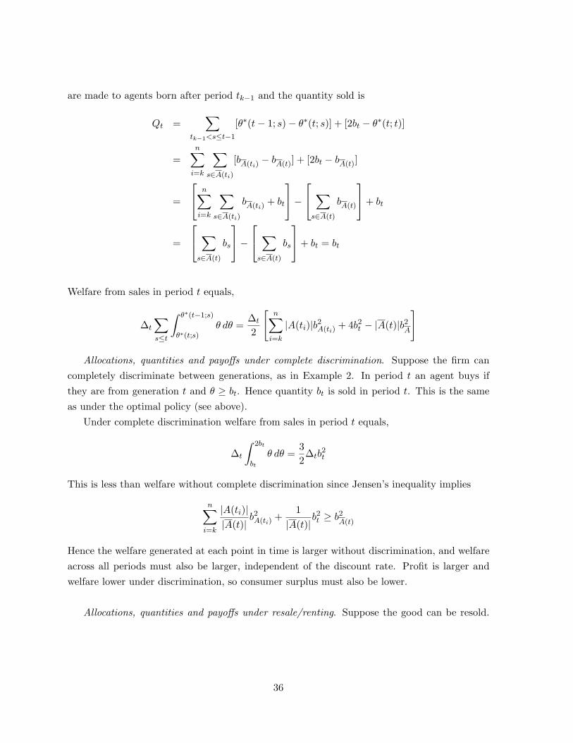
are made to agents born after period tk−1 and the quantity sold is

Qt =∑

tk−1<s≤t−1

[θ∗(t− 1; s)− θ∗(t; s)] + [2bt − θ∗(t; t)]

=n∑

i=k

∑

s∈A(ti)

[bA(ti)− bA(t)] + [2bt − bA(t)]

=

n∑

i=k

∑

s∈A(ti)

bA(ti)+ bt

−

∑

s∈A(t)

bA(t)

+ bt

=

∑

s∈A(t)

bs

−

∑

s∈A(t)

bs

+ bt = bt

Welfare from sales in period t equals,

∆t

∑

s≤t

∫ θ∗(t−1;s)

θ∗(t;s)θ dθ =

∆t

2

[n∑

i=k

|A(ti)|b2A(ti)

+ 4b2t − |A(t)|b2

A

]

Allocations, quantities and payoffs under complete discrimination. Suppose the firm cancompletely discriminate between generations, as in Example 2. In period t an agent buys ifthey are from generation t and θ ≥ bt. Hence quantity bt is sold in period t. This is the sameas under the optimal policy (see above).

Under complete discrimination welfare from sales in period t equals,

∆t

∫ 2bt

bt

θ dθ =32∆tb

2t

This is less than welfare without complete discrimination since Jensen’s inequality implies

n∑

i=k

|A(ti)||A(t)| b

2A(ti)

+1

|A(t)|b2t ≥ b2

A(t)

Hence the welfare generated at each point in time is larger without discrimination, and welfareacross all periods must also be larger, independent of the discount rate. Profit is larger andwelfare lower under discrimination, so consumer surplus must also be lower.

Allocations, quantities and payoffs under resale/renting. Suppose the good can be resold.

36

Theorem 3 implies that the time t cutoff is given by

θRt =

1t

∑

s≤t

bs

The quantity sold up to period t is∑

s≤t(2bt − θRt ) =

∑s≤t bs. Hence quantity bt is sold in

period t. This is the same as without resale (see above).Welfare with resale in period t is

(∆t −∆t+1)∑

s≤t

∫ 2bt

θRt

θ dθ = (∆t −∆t+1)∑

s≤t

[2b2

t − [θRt ]2

]

In rental terms, welfare in period t without resale is

(∆t −∆t+1)∑

s≤t

∫ 2bt

θ∗(t;s)θ dθ = (∆t −∆t+1)

∑

s≤t

[2b2

t − [θ∗(t; s)]2]

Welfare is then greater with resale since

∑

s≤t

[θ∗(t; s)]2 ≥ 1t

∑

s≤t

θ∗(t; s)

2

=1t

∑

s≤t

bs

2

=1t

[tθR

t

]2=

∑

s≤t

[θRt ]2

where the first equality uses the fact that the firm sells quantity bt each period under Theorem1. Intuitively, welfare is higher with resale since the same quantity is allocated more efficiently.With resale, profits are lower and welfare higher, so consumer surplus is also higher.

A.4 Best–Price Policy with Resale: Example 9

Suppose T = 2, δ is constant and A2 holds.15 For convenience let us drop the “BP” superscripts.Fix the period 1 price and cutoff (p1, θ

∗1). In period 2 the firm chooses p2 inducing cutoff

θ∗2 = p2. p2 is chosen to maximise

Π2 = p2[F 1,2(p2)− F 1(θ∗1)]− F 1(θ∗1)max0, p1 − p2

The optimal choice of p2 is then given by

p∗2 = m−11,2(0) if p1 ≥ m−1

1,2(0) (A.1)

< m−11,2(0) if p1 < m−1

1,2(0)

15A full characterisation of the subgame perfect equilibrium can be obtained from the author.

37

Thus p∗2 ≤ maxp1,m−11,2(0).

In period 1 consumers’ purchasing decision depends upon the current price p1 and theirexpectation of the second period price p2. The utility of agent θ∗1 who buys in period 1 andsells in period 2 is

(1− δ)θ∗t − p1 + δp2 + δ max0, p1 − p2 (A.2)

Since agent θ∗1 must be indifferent between buying and not, setting (A.2) equal to zero yieldsthe first period price

p1 = (1− δ)θ∗1 + δ maxθ∗1, p2 (A.3)

Fix θ∗1 and consider two cases. First suppose θ1 ≥ m−11,2(0). Equation (A.3) implies

p1 ≥ θ∗1 ≥ m−11,2(0). Equation (A.1) implies θ∗2 = p∗2 = m−1

1,2(0).Second suppose θ∗1 < m−1

1,2(0). Since p∗2 ≤ m−11,2(0), equation (A.3) implies p1 < m−1

1,2(0).Equation (A.1) implies θ∗2 = p∗2 < m−1

1,2(0).Now let us examine the optimal period 1 cutoffs. First, suppose demand is decreasing.

The firm can choose θ∗1 = m−11 (0) ≥ m−1

1,2(0) which induces θ∗2 = m−11,2(0) in period 2. This

implements the commitment optimum and is therefore optimal in period 1.Next, suppose demand is not decreasing. If the firm chooses θ∗1 = m−1

1 (0) < m−11,2(0) the

optimal period 2 choice is p∗2 < m−11,2(0) and the firm overproduces. Hence the commitment

optimum is not implementable. It can be shown that the period 2 cutoff θ∗2 is increasing inperiod 1 cutoff θ∗1. It follows that the optimal period 1 cutoff satisfies θ∗1 > m−1

1 (0).

38

References

Biehl, A. R. (2001): “Durable-Goods Monopoly with Stochastic Values,” RAND Journal ofEconomics, 32(3), 565–577.

Board, S. (2004): “Selling Options,” Working paper, University of Toronto.

Bulow, J. (1982): “Durable-Goods Monopolists,” Journal of Political Economy, 90(2), 314–332.

Butz, D. A. (1990): “Durable-Good Monopoly and Best-Price Provisions,” American Eco-nomic Review, 80(5), 1062–1076.

Chow, Y. S., H. Robbins, and D. Siegmund (1971): Great Expectations: The Theory ofOptimal Stopping. Houghton Mifflin.

Coase, R. H. (1972): “Durability and Monopoly,” 15(1), 143–149.

Conlisk, J. (1984): “A Peculiar Example of Temporal Price Discrimination,” EconomicsLetters, 15(1–2), 121–126.

Conlisk, J., E. Gerstner, and J. Sobel (1984): “Cyclic Pricing by a Durable GoodsMonopolist,” Quarterly Journal of Economics, 99(3), 489–505.

Davidson, J. (1994): Stochastic Limit Theory. Oxford University Press, Oxford.

Hendel, I., and A. Lizzeri (1999): “Adverse Selection in Durable Goods Markets,” AmericanEconomic Review, 89(5), 1097–1115.

Klass, M. (1973): “Properties of Optimal Extended–Valued Stopping Rules for Sn/n,” Annalsof Probability, 1(5), 719–757.

Laffont, J.-J., and J. Tirole (1996): “Pollution Permits and Compliance Strategies,” Jour-nal of Public Economics, 62(1–2), 85–125.

Landsberger, M., and I. Meilijson (1985): “Intertemporal Price Discrimination and SalesStrategy under Incomplete Information,” RAND Journal of Economics, 16(3), 424–430.

Levhari, D., and R. S. Pindyck (1981): “The Pricing of Durable Exhaustible Resources,”Quarterly Journal of Economics, 96(3), 365–378.

Milgrom, P., and I. Segal (2002): “Envelope Theorems for Arbitrary Choice Sets,” Econo-metrica, 70(2), 583–601.

39

Myerson, R. (1981): “Optimal Auction Design,” Mathematics of Operations Research, 6(1),58–73.

Rotemberg, J. J., and M. Woodford (1999): “The Cyclical Behaviour of Prices and Costs,”in Handbook of Macroeconomics, pp. 1051–1135, (J.B. Taylor and M. Woodford eds.).

Royden, H. L. (1988): Real Analysis, Third Edition. Prentice Hall, New Jersey.

Rust, J. (1985): “Stationary Equilibrium in a Market for Durable Assets,” Econometrica,53(4), 783–806.

(1986): “When is it Optimal to Kill off the Market for Used Durable Goods?,” Econo-metrica, 54(1), 65–86.

Segal, I. (2003): “Awarding Monopoly Franchises,” American Economic Review, 93(3), 509–529.

Sobel, J. (1991): “Durable Goods Monopoly with Entry of New Consumers,” Econometrica,59(5), 1455–1485.

Sobel, J., and I. Takahashi (1983): “A Multistage Model of Bargaining,” Review of Eco-nomic Studies, 50(3), 411–426.

Stokey, N. L. (1979): “Intertemporal Price Discrimination,” Quarterly Journal of Economics,93(3), 355–371.

Tirole, J. (1988): The Theory of Industrial Organization. MIT Press, Cambridge, Massa-chusetts.

Topkis, D. M. (1998): Supermodularity and Complimentarity. Princeton University Press,New Jersey.

Waldman, M. (1996): “Durable Goods Pricing When Quality Matters,” Journal of Business,69(4), 489–510.

Wang, R. (2001): “Optimal Pricing Strategy for Durable-Goods Monopoly,” Journal of Eco-nomic Dynamics and Control, 25(5), 789–804.

40