RAND Journal of Economics Vol. 39, No. 2, Summer 2008

pp.530-546

Durable goods and residential demand for energy and water: evidence from a field trial

Lucas W. Davis*

This article describes a household production model in which energy-efficient durable goods cost less to operate so households may use them more. The model is estimated using household level data from afield trial in which participants received high-efficiency clothes washers free of charge. The estimation strategy exploits this quasi-random replacement of washers to derive

precise estimates of the household production technology and a demand function for clothes

washing. During the field trial, households increased clothes washing on average by 5.6% after receiving a high-efficiency washer, implying a price elasticity of ?.06. The complete model is used to evaluate the cost-effectiveness of recent changes in minimum efficiency standards for clothes washers.

1. Introduction

The energy efficiency of household durable goods has improved dramatically since the 1970s. Between 1972 and 2001, average gasoline consumption per mile for new automobiles decreased 49% and average electricity consumption of central air conditioners and refrigerators decreased 44% and 56%, respectively.l Despite these innovations, energy consumption per capita in the United States decreased only 3% during the same period.2 One reason for the small decrease is that households in 2001 were driving more, keeping their homes cooler in the summer, and

owning larger refrigerators. In part, these changes in utilization were a reaction to the efficiency improvements. Improvements in energy efficiency decrease the price of using durable goods

which may lead to higher utilization. It is important to take this behavioral response into account when evaluating the cost

effectiveness of policies that encourage energy efficiency.3 The argument for these policies is

* University of Michigan; lwdavis@umich.edu.

This article is based on my Ph.D. dissertation at the University of Wisconsin. I thank John Kennan, Maurizio Mazzocco,

Gary Solon, Matthew White, the editor, and several anonymous referees as well as seminar participants at Wisconsin,

Harvard, Chicago GSB, Stanford, Columbia, and Wharton for helpful comments. Thanks also to D. Tom Rizy at Oak

Ridge National Laboratory for providing the records from the Bern Washer Study. This research was made possible through an NICHD Training Grant (T32 HD07014) and the Center for Demography Ecology, which receives core support from the National Institute for Child and Human Development (R24 HD 47873). Generous financial support was also

provided by the Christensen Award in Empirical Economics. 1 U.S. Department of Transportation (2004); Nadel (2002). 2 U.S. Department of Energy (2005a). 3 There are many examples of public policies that encourage residential energy efficiency in the United States

including federal minimum efficiency standards, the Credit for Energy Efficient Appliances, and the Alternative Motor

Vehicle Credit.

530 Copyright ? 2008, RAND.

DAVIS / 531

that energy consumption imposes social costs that households do not consider when choosing which durable goods to purchase. Perhaps most important, the combustion of fossil fuels causes

emissions of carbon dioxide, the principal greenhouse gas associated with climate change.

However, the effectiveness of these policies in reducing energy consumption depends on the

price elasticity of utilization. The larger the price elasticity, the less effective these policies are

at lowering energy consumption. Some critics of these policies have argued that high-efficiency durable goods actually increase energy consumption, implicitly claiming that the price elasticity of utilization exceeds one.4

In order to evaluate these claims, this article describes a model of residential energy and water demand that incorporates this behavior. Following Dubin and McFadden (1984), demand for

durable goods and demand for energy and water are model jointly as the solution to a household

production problem. In the model, inputs such as energy and water are used with durable goods to

produce services that the household cares about. The analysis highlights a simultaneity problem that makes the price elasticity of utilization difficult to measure in most contexts. Households take

expected utilization into account when deciding which durable goods to purchase. As a result, households with high demand for utilization are more likely to purchase energy-efficient durable

goods and thus have a lower marginal cost of utilization. The article addresses this endogeneity by examining household behavior during a field trial

in which participants received a high-efficiency clothes washer free of charge. This quasi-random replacement of washers during the field trial introduces plausibly exogenous variation in the households' production technology, making it possible to derive unbiased estimates of the price elasticity of utilization. As demonstrated in the article, when this simultaneity is ignored, estimates of the price elasticity are biased away from zero. The only previous study to exploit a field trial in

this way is Dubin et al. (1986), who examine a random sample of homes in Florida that received free upgraded attic insulation and other free energy efficiency improvements.

The results document large decreases in energy and water consumption per cycle when the households receive high-efficiency clothes washers. The estimates of the production technology indicate that the high-efficiency washers use an average of 48% less energy and 41% less water than conventional washers per cycle. The implied estimates of marginal cost are used to estimate a demand equation for clothes washing. During the field trial, the average household increased clothes washing by 5.6% after receiving a high-efficiency clothes washer. After controlling for weather and other covariates, the price elasticity of clothes washing is ?.06, a magnitude that is smaller than estimates in the literature for central heating and air conditioning. The estimate is similar across a variety of alternative specifications. Thus, for clothes washers, it appears that

only a small portion of the gains in energy and water efficiency are offset by increased utilization. The estimated parameters are used to examine the cost-effectiveness of recent changes

in minimum efficiency standards for clothes washers. Although evidence from the field trial is valuable for studying utilization behavior, it is less helpful for studying adoption behavior because households are not observed purchasing washers. In lieu of a formal empirical model of the purchase decision, reasonable assumptions about production costs, washer lifetimes, and the discount rate are used to derive preliminary measures of the costs and benefits of the increased

standards, as well as the distribution of benefits across households. The results suggest that most households are made better off buying a washer that meets the 2007 standard. When the social benefit of reduced carbon emissions is included in the analysis, it appears that the minimum standard does meet a cost-benefit test.

The format of the article is as follows. Section 2 describes the household production model and discusses the endogeneity problem. Section 3 describes the data from the field trial and

4 "Energy Conservation Is a Waste," commentary by H. Inhaber, Wall Street Journal, July 28, 1997. "Conservation

Wastes Energy," commentary by K. Strassel, Wall Street Journal, May 17, 2001."Disappearing Energy Crisis in the US? Paul Georgia on NPR," interview with Paul J. Georgia (policy analyst, Competitive Enterprise Institute), Talk of the

Nation, National Public Radio, July 24, 2001.

?RAND 2008.

532 / THE RAND JOURNAL OF ECONOMICS

provides background for the empirical analysis. Section 4 specifies a functional form for the production technology, solves the cost-minimization problem, and presents estimates of the

production technology. Section 5 describes and estimates a demand function for clothes washing. Estimates of the price elasticity of utilization as well as implied price elasticities for inputs are

presented and discussed. Section 6 presents the cost-benefit analysis and Section 7 provides concluding remarks.

2. A model of household production with durable goods This section describes a model of durable good purchase and utilization similar to the

model described by Dubin and McFadden (1984). In the model, demand for energy and water is derived from demand for household services that are produced in the home according to a household production technology. The model is general enough to describe a wide variety of household durable goods or complete durable good portfolios. The analysis clarifies the source of the endogeneity bias described above and shows how quasi-random variation in household durable good characteristics during field trials can be used to derive unbiased estimates of the

price elasticity of utilization and other parameters of the model. Households are assumed to choose the durable good portfolio that yields the highest level

of utility,

max{V(&x),...,V(&j)}, (1) /el,...,/

where V is a conditional indirect utility function and 0y is a vector of observed characteristics for durable good portfolioy. The decision of which durable goods to purchase is made taking into account that whichever durable goods are purchased, they will be operated at the optimal level of utilization. The durable good purchase decision is solved by evaluating the conditional indirect

utility function for each alternative,

V(@j) = max U(zx,z2\rj) n) {x,t,z2} v '

s.t. zx =f(x,t\Gj)

px +z2 = tmw -r(?j)

t + tm = T.

As in the original household production model described by Becker (1965), this model formalizes the relationship between market inputs and services produced within the home. Household utility is defined over household services zx and a composite good z2. The price of the composite good is normalized to one. Parameter t] varies across households reflecting differences in the relative value a household places on household services zx. The production function for zx is denoted/ and depends on a vector of inputs, x, and time used in household production, t. The parameters of the technology depend on the characteristics of the household's durable goods, 07. Households evaluate expenditure on inputs based on the utility derived from zx and the disutility of foregone consumption of composite good z2. The budget constraint depends on a vector of input prices/?, the market wage w, and capital cost r that is a function of the characteristics of the durable good portfolio. Time allocated to household production t and market work tm cannot exceed the total time endowment T.

Let C(p, w,zx\ 0;) denote the minimum cost of producing zx given input prices/?, wage w, and durable good characteristics 0y,

C(p, w, zx | 0y) = min px + tw (3)

{x,t}

s.t. zx = f(x,t I ?j).

?RAND 2008.

DAVIS / 533

Furthermore, let the marginal cost of producing zx be denoted n,

dC(p,w,zx \@j) iz(p, w I 0;) =-. (4)

ozx

Pollak and Wachter (1975) show that if the production technology exhibits constant returns

to scale and there is no joint production, then marginal cost does not depend on the level of

production.5 This is a significant analytical improvement because the household's problem may be treated as a classic demand problem,

max U(zx,z2, \ rj) (5) {z\,z2}

s.t. n(p, w | Sj)zx + z2 = wT - r(Sj).

In this reformulation of the problem, marginal cost plays the traditional role of a price and the

problem can be solved as usual by equating the marginal rate of substitution with the price ratio.6

Under these conditions, the solution to the household's utility-maximization problem is

described by the demand function for z x,

zx =zx(7Tj,yj | rj). (6)

Demand for household services zx depends on its marginal cost, ttj = n(p, w | 0y), and net

income, y}=wT ? r (07), both of which depend on the characteristics of the household's durable

good portfolio, 07. This description highlights the simultaneity problem that makes the demand function difficult

to estimate empirically. Demand depends on parameter r] that varies across households reflecting differences in the relative value a household places on household services. However, households

also take r\ into account when deciding which durable goods to purchase. As a result, marginal cost is endogenous in the demand equation and attempts to estimate the demand for utilization

using cross-sectional variation in marginal cost will be biased. In purchasing durable goods, households with high demand for utilization tend to purchase high-efficiency durable goods. As a result, marginal cost will tend to be negatively correlated with demand, causing estimates of the

price elasticity,

dzx(7tj,yj | rj) Ttj

ditj zx(7tj,yj | riY

to be biased away from zero. For example, consider the case of vehicles. Households with high demand for driving will tend to purchase vehicles for which the marginal cost of driving is low. This causes a negative correlation between the marginal cost of driving and miles traveled. An econometrician who fails to account for this endogeneity when measuring the effect of marginal cost on driving will overstate the price elasticity.

The standard approach for addressing this endogeneity is to describe the durable good choice problem explicitly using a discrete choice model. In the approach originated by Dubin and McFadden (1984), choice probabilities from the purchase decision are used as an instrument for durable good holdings in estimating the utilization decision. This two-step approach has become the standard in micro-simulation models of energy demand such as the U.S. Department of Energy's National Energy Modeling System. This article takes an alternative approach that examines demand for household services during a field trial. The field trial introduces variation in marginal cost that is uncorrelated with rj and thus can be used to derive unbiased estimates of the price elasticity. The empirical analysis focuses on the utilization decision (5), rather than

5 Joint production occurs when the cost of producing a particular household service depends on the level of

production of another household service. Joint production arises frequently when time is an input in the production function.

6 In the presence of nonconstant returns to scale, marginal cost depends on the level of production and the feasible set is no longer a straight line. As a result, even if preferences are strictly convex, there may be multiple solutions and the demand function need not be continuous inp and w.

?RAND 2008.

534 / THE RAND JOURNAL OF ECONOMICS

the durable good choice decision (1). Therefore, the results can be used to assess the change in energy and water consumption of households that adopt high-efficiency washers, but they cannot be used to predict adoption patterns.

3. Description of the field trial The empirical analysis in the article focuses on clothes washers. Clothes washing is a

particularly lucid example of a household production process where demand for energy and other inputs is derived from demand for consumption of a household service. In addition, clothes

washing is of significant independent interest because of the high level of energy and water

consumption associated with it. According to the 2001 Residential Energy Consumption Survey, households in the United States use 1 trillion gallons of water and 186 trillion btus of energy annually washing clothes. Inside the home, clothes washing and drying accounts for 10.1% of total energy consumption and 21.5% of total water consumption.

Beginning in the late 1990s, high-efficiency washers were introduced in the United States that have the potential to reduce this energy and water consumption dramatically. Whereas conventional washers suspend clothes in a tub of water and agitate them along a vertical axis for

washing and rinsing, high-efficiency washers tumble clothes on a horizontal axis through a pool of water at the bottom of the tub. In large part because they use less hot water, high-efficiency washers also use less energy. Engineering studies demonstrate that high-efficiency washers use

up to 40% less water and up to 60% less energy per cycle than conventional washers. These large savings led the Department of Energy to conduct a field trial of a high-efficiency

clothes washer in Bern, Kansas (population 200) in 1997. Sponsored by Maytag and conducted by Oak Ridge National Laboratory, the study provided participants with free high-efficiency clothes washers in order to evaluate the energy and water consumption characteristics of these washers under real-world conditions.7 Bern was selected from among a list of potential sites identified with the cooperation of the National Rural Water Association. The project coordinators wanted a location small enough that they could replace a high proportion of all washers within a particular

water utility system. This allowed them to assess the municipal impact of the washers as well as the household-level effect. Bern is a farming community in the northeast corner of Kansas.

According to the 2000 Census, median household income in Bern is 4% below the US. median. All residents of Bern and the surrounding rural water district were invited to participate in

the study. In order to participate, households were required to currently own a clothes washer and

agree to keep records of their clothes-washing behavior before and after receiving the new clothes washer. Ninety-eight out of 171 households in the water district chose to participate. Because the empirical strategy controls for unobserved household-specific heterogeneity, the estimate of the price elasticity will not be biased if households with particularly inefficient machines or households with high demand for clothes washing were more likely to participate than other households. However, the estimate of the price elasticity will be biased if households that chose to participate are systematically more or less responsive to changes in marginal cost than other households.

Before participating in the study, households were made aware of the efficiency character istics of the new washers. At a town meeting on May 27 in the Bern High School gym, project

managers met with participants to explain that the goal of the study was to measure the energy and water consumption characteristics of high-efficiency clothes washers, and that in engineering studies these washers had been shown to decrease energy consumption by up to 60% and water

consumption by up to 40%. This is similar to the information typically available to households

buying a high-efficiency washer. Since 1980, the U.S. Federal Trade Commission's Appliance Labeling Rule has required manufacturers to attach yellow and black "Energy Guide" labels to most major home appliances including clothes washers. These labels provide an estimate of

7 See Tomlinson and Rizy (1998) for more information about the Bern Washer Study.

?RAND 2008.

DAVIS / 535

TABLE 1 Bern Washer Study, Descriptive Statistics

Phase 1 Phase 2

Number of households 95 95

Number of days 51 91

Total number of wash cycles 6,559 11,674

Total number of pounds of clothes washed 43,339 81,752 Proportion of household days with clothes washing .53 .56

Mean number of pounds washed per day per household 8.95 9.46

Mean number of wash cycles per day per household 1.35 1.35

Mean hot water use per cycle (gallons) 10.4 4.3

Mean cold water use per cycle (gallons) 27.8 19.4

Mean electricity use for washer motor per cycle (kwh) .22 .10

Mean propane use for water heating per cycle (kwh) 3.59 1.41

Mean electricity use for water heating per cycle (kwh) 1.94 0.87

Mean electricity use for drying clothes per cycle (kwh) 2.00 1.85

Mean detergent use per cycle (ounces) 3.97 3.99

Water prices in Bern (per 1000 gallons) $2.50 $2.50

Electricity rate (per kwh) $.077 $.077 Propane rate (per kwh) $ .029 $ .029

Detergent price (per ounce) $ .085 $.000 Mean maximum daily temperature (Fahrenheit) 88.1 77.8

Mean daily precipitation (inches) . 105 .124

annual energy consumption on a scale showing a range of similar models and estimated annual

operating cost based on national average utilization levels and national average energy rates. The field trials took place between June and November 1997. Between June 2 and June 6,

water monitoring instrumentation was installed on the current washers of all participants. During the next two months, households recorded information about each wash cycle including water

readings for hot and cold water usage and load weights before and after washing, as well as

information about detergent usage, machine settings, and self-reported measures of satisfaction with cleaning performance and dampness. The project managers designed data collection to minimize misreporting. Water consumption was recorded cumulatively and wash cycle records were collected and analyzed periodically during the course of the project. This allowed the

project managers to identify and remedy reporting problems. In addition, in order to standardize

measurements, households were provided with identical scales, laundry baskets, and measuring cups.

Between July 28 and August 1, all washers were replaced with identical Maytag Neptune high-efficiency washers. For the next three months, households continued to record information about their wash cycles. Throughout the analysis, "phase 1" denotes the period before installation of the high-efficiency washers and "phase 2" denotes the period after installation. During phase 2, the households received free of charge a low-sudsing laundry detergent designed for high efficiency clothes washers. Households paid for their own energy and water throughout the

study.

Table 1 presents descriptive statistics. The data set includes detailed records of over 18,000 wash cycles and over 125,000 total pounds of clothes washed. The sample includes all wash cycles recorded between June 7 and July 27 and between August 2 and October 31. The sample excludes records from washers replaced at the Bern High School, Bern Meat Plant, Bern Laundromat, Bern Veterinarian Clinic, and three households that reported wash cycles in one phase only. From the remaining 95 households, 192 out of 18425 total wash cycles were excluded because of

miscoding. Specifically, 57 cycles were excluded because the date was missing, 76 observations were excluded because hot water usage was miscoded, and 59 observations were excluded because cold water usage was miscoded.

?RAND 2008.

536 / THE RAND JOURNAL OF ECONOMICS

FIGURE 1

WATER AND ENERGY CONSUMPTION PER CYCLE

? _ iirsiffifltllliHilVlltlfV 111 illllflllllw ,im.?nI,*kV?i.%f?,...,.?. H-1-1-\-1-1?

10 20 30 40 50 60 Water Consumption per Cycle in Gallons

^^H Front-Loading Washers ^#S?H Conventional Washers

CO - I

L,-,-!-!_ 0 5 10 15

Electricity Consumption per Cycle in kwh

HHH Front-Loading Washers /&'. Conventional Washers

Energy and water consumption per cycle decreased substantially between phases. Figure 1

plots histograms of energy and water consumption per cycle. Energy usage for each component of production is calculated following Tomlinson and Rizy (1998) using hot water usage, water

temperature, hot water heater type, the difference in clothing weight before and after washing, and

engineering estimates of per-cycle motor electricity consumption by model. Reported propane usage for water heating is for the 65 households with propane water heaters. Reported electricity usage is for the 30 households with electric water heaters. Table 1 also includes prices and weather characteristics. Water rates are marginal water rates in Bern during the summer of 1997 for the first 10,000 gallons. Electricity and propane rates are average residential prices for Kansas for 1997 from the U.S. Department of Energy, "State Energy Consumption, Price,

?RAND 2008.

DAVIS / 537

and Expenditure Estimates." Detergent price in phase 1 is the average price per ounce of 35 common detergents reviewed by Consumer Reports in February 1995. No distinction is made

between liquid ($.083/ounce) and powder ($.086/ounce) detergents. Maximum daily temperature and daily rainfall are from the NOAA National Virtual Data System for Centralia, KS, a town

that is 27 miles south of Bern. In addition to energy and water efficiency, there are a number of potentially important

differences between high-efficiency washers and conventional washers. First, high-efficiency washers tend to be more gentle on clothes because they do not have an agitator. Although the

difference is subtle, this could cause households to increase clothes washing because the cost

in terms of wear and tear has decreased or because a wider range of clothes can be washed.

Second, high-efficiency washers tend to have a larger tub capacity than conventional washers. The high-efficiency washers used in the field trial have a tub volume of 3.3 cubic feet compared to an average tub volume in phase 1 of 2.8 cubic feet. This difference in capacity could cause

households to increase clothes washing because larger items can be washed or because washing

requires less time. The empirical analysis does not model these differences, and thus the results

may overstate the responsiveness of demand to changes in energy and water prices. Between

phase 1 and phase 2, the average number of pounds of clothes washed per day per household increased from 8.95 to 9.46. Thus, on average, households increased clothes washing by 5.6% after receiving the new washers. This increase occurred almost entirely in the number of pounds per wash cycle, not in the number of cycles. Had capacity and other characteristics of the washers not changed at the same time, the increase in utilization might have been even smaller.

4. The production technology This is one of the first studies to estimate a household production technology explicitly.

Despite the analytical advantages of this approach, household production models have received little attention empirically. Instead, most studies focus on household demand for inputs rather than on the underlying household services from which demand for the inputs is derived. The

main reason household production models have not received more empirical attention is that

consumption of services produced within the home is typically not observed. An attractive feature of many field trials is that inputs and outputs are recorded. In this particular field trial, measures are recorded of energy consumption, water consumption, detergent consumption, and

pounds of clothes washed. Formally describing the household production technology increases the predictive power of the model by restricting the pattern of substitution among inputs, making it possible to infer price elasticities for energy, water, and detergent consumption derived from clothes washing.

This section describes the functional form used for the production technology, solves the cost-minimization problem, and presents estimates of the input demand functions. Clean clothes, zx, are produced in the home using a clothes washer, clothes dryer, hot water heater, water, energy,

detergent, and time. As described in the model, zx is assumed to be a source of direct utility for the household. Production is described using a Leontief production function. This choice of

production function implies that inputs are required proportionally in the production of clothes

washing. The production function, /, describes the number of pounds of clean clothes that are

produced for a given level of water xx, energy for the motor x2, energy for water heating jc3, energy for drying x4, detergent x5, and time t:

/Y ^ I /^\ f *1 *2 *3 X4 X5 ^ 1 /ox zx = f(xx,x2,x3,x4,x5,t I 0)

= min{ ?, ?,

? ,?,?,

? }. (8)

(ax a2 a3 a4 a5 a6 J

The parameters of the production technology, 0 = {ax, a2, o?3, a4, a5, a6}, reflect the

characteristics of the durable goods owned by the household. For example, if the clothes washer is water efficient, then a x is low. Households solve the cost-minimization problem for clothes

washing by allocating all inputs proportionally,

?RAND 2008.

538 / THE RAND JOURNAL OF ECONOMICS

TABLE 2 Production Function Estimates?Inputs Required per Pound

Phase 1 Phase 2

Mean Standard Deviation Mean Standard Deviation

a i Water (gallons) 5.56 1.90 3.27 .901

a2 Electricity for motor (kwh) .031 .011 .013 .004 a3a Propane for water heating (kwh) .501 .252 .193 .128 a3b Electricity for water heating (kwh) .319 .100 .131 .044

a4 Electricity for drying (kwh) .294 .055 .258 .042

a5 Detergent (ounces) .580 .261 .545 .196

7t Marginal cost per pound $.11 .03 $.04 .01 Cost per cycle $.72 .24 $.26 .09

Marginal cost per pound (including time) $.52 .03 $.45 .01 Cost per cycle (including time) $3.46 1.34 $3.16 1.38

Xl __ Xl _ *3 _ *4 _ Xs ? * ? (Q\ ax a2 a3 a4 a5 a6

The production technology is estimated using the conditional demand functions:

X\ic ?

\irz\ic i ?\ic

x2ic = a2irz\ic + ?2ic

X3ic = Oi3iTZUc + ?3ic (10)

X^ic ?

^Aixz\ic "t" &4ic

Xsic = & Sitz lie "T" Gsic*

Here / indexes households, c indexes wash cycles, and r indexes phase. The input demand function for time is excluded and discussed below. This system of equations is estimated separately for each household and each phase using systems least squares. For each household, there are five parameters for phase 1 and five parameters for phase 2. The error term is assumed to be measurement error orthogonal to the level of output. Substituting the conditional demand functions into the cost function and dividing by zx yields marginal cost,

7T?r = P\OL\ix + PlOtlir + P&lix + A?4/r + P&Six- 0 1)

Table 2 presents estimates of the production technology. The parameters vary across households and phase. For example, the mean value for ax in phase 1 is 5.56 and the standard deviation across households is 1.90. The parameters demonstrate the improvements in energy and water

efficiency realized with the installation of the high-efficiency washers. The mean number of gallons of water required to produce one pound of clean clothes

decreased from 5.56 in phase 1 to 3.27 in phase 2. The parameters for energy usage indicate similar efficiency improvements. The energy savings are substantial for households with both

propane water heaters, a3a, and electric hot water heaters, a3b. On average, the estimates imply that households used 41% less water and 48% less energy per cycle. Equation (11) implies that

during the field trial, the marginal cost of clothes washing decreased from $. 11 to $.04 per pound, a change of 65%.

Clothes washing is one of the most time-intensive components of household production. In contrast, previous studies of residential energy demand have tended to focus on heating and cooling equipment, where time is a much smaller component of the production process.8

8 See Hausman (1979), Dubin and McFadden (1984), Dubin et al. (1986), and Bernard et al. (1996).

?RAND 2008.

DAVIS / 539

According to the EPA Time Use Survey (1994), among household production activities, only child care and food preparation are more time intensive. Households report spending an average of

7.56 minutes per household member per day for "clothing care." For a family of four, this implies almost four hours per week. Using the average number of pounds of clothes washed per day per household during phase 1 (8.95) and the average number of members per household in Bern (2.58), the time-use estimates imply a time component of .05 hours per pound. Adopting the mean hourly

wage in Kansas in 1997 ($12.08) from the Bureau of Labor Statistics' Occupational Employment Statistics Survey, the cost estimates reported in Table 2 demonstrate that time costs increase the cost of clothes washing considerably. In phases 1 and 2, the cost of time represents 79% and 92%

of total costs, respectively. Throughout the analysis that follows, elasticities are reported with

respect to the marginal cost of clothes washing excluding time. For most counterfactuals, this is the elasticity that is most useful. Also, this facilitates the comparison with previous estimates in the literature for other durable goods. When elasticities are calculated with respect to total

costs, the estimates are larger because the same variation in demand is now explained by a smaller relative change in prices. In addition to clothes washing, there are many production processes in the home that include a substantial time component. For these services, the price elasticity with

respect to the price of energy and other non-time inputs will appear small.

5. Demand for clothes washing Main results. As described in Section 2, the solution to the household's utility-maximization

problem may be described by the demand equation. Demand for clean clothes zXit in pounds by household / on day / is postulated to depend linearly on marginal cost nit, a vector of covariates

Xit, unobserved time-invariant household characteristics rji9 and unobserved household-specific time-varying factors coit,

zut = Yo + Yinu + YiXit + r\i + coit. (12)

Dubin and McFadden (1984) show that a demand equation with this functional form can be derived from an internally consistent utility-maximization problem by applying Roy's identity to a conditional indirect utility function of the generalized Gorman polar form.

The dependent variable is zero for 45% of all observations and then continuously distributed over positive values. Accordingly, a Tobit model is used for the main results. With the Tobit

model, the household fixed effects are estimated explicitly along with y0, yx, and y2. It has

long been recognized that with a Tobit model, estimation of fixed effects introduces an incidental

parameters problem, leading to inconsistent parameter estimates for fixed T and n -> oo. However, in this case, T = 142, so the magnitude of the inconsistency is likely to be small. Alternative

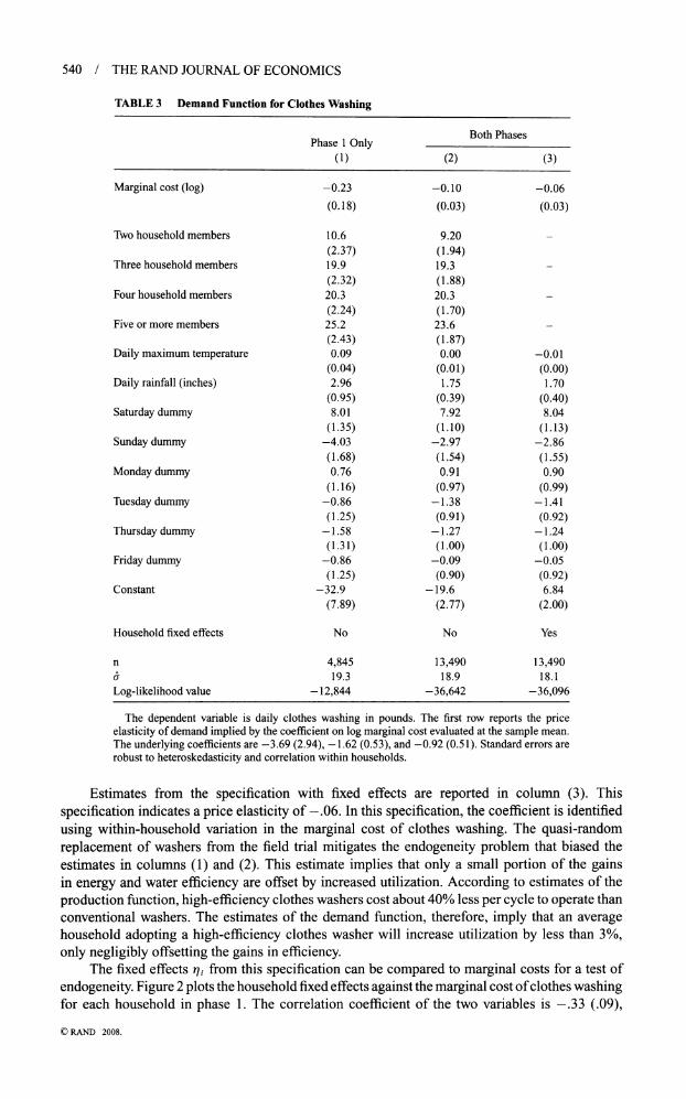
specifications are considered in the next subsection. Table 3 presents estimates of the demand function. Column (1) reports estimates from

a specification that excludes observations from after the households received high-efficiency washers. As in a conventional cross-sectional analysis, in this specification the price elasticity is identified from differences in durable good holdings across households. In this specification, the price elasticity of clothes washing is ?.23. This relatively large estimate is consistent with the discussion in Section 2 that argued that endogeneity bias will tend to bias cross-sectional estimates of the price elasticity away from zero. Households with high demand tend to purchase high-efficiency durable goods, causing a spurious negative correlation between marginal cost and the error term.

Column (2) reports estimates from a specification that includes observations from both before and after households receive high-efficiency washers but again excludes household fixed effects. This specification represents an improvement over the previous specification because much of the variation in marginal cost comes from the variation between phases. Because this variation is not correlated with the unobserved determinants of demand, the estimate of the price elasticity suffers less from endogeneity bias.

?RAND 2008.

540 / THE RAND JOURNAL OF ECONOMICS

TABLE 3 Demand Function for Clothes Washing

Both Phases Phase 1 Only _

_(1)_(2)_(3) Marginal cost (log) -0.23 -0.10 -0.06

(0.18) (0.03) (0.03)

Two household members 10.6 9.20 -

(2.37) (1.94) Three household members 19.9 19.3

(2.32) (1.88) Four household members 20.3 20.3 -

(2.24) (1.70) Five or more members 25.2 23.6 -

(2.43) (1.87) Daily maximum temperature 0.09 0.00 ?0.01

(0.04) (0.01) (0.00) Daily rainfall (inches) 2.96 1.75 1.70

(0.95) (0.39) (0.40) Saturday dummy 8.01 7.92 8.04

(1.35) (1.10) (1.13) Sunday dummy -4.03 -2.97 -2.86

(1.68) (1.54) (1.55) Monday dummy 0.76 0.91 0.90

(1.16) (0.97) (0.99) Tuesday dummy -0.86 -1.38 -1.41

(1.25) (0.91) (0.92) Thursday dummy -1.58 -1.27 -1.24

(1.31) (1.00) (1.00) Friday dummy -0.86 -0.09 -0.05

(1.25) (0.90) (0.92) Constant -32.9 -19.6 6.84

(7.89) (2.77) (2.00)

Household fixed effects No No Yes

n 4,845 13,490 13,490 o 19.3 18.9 18.1

Log-likelihood value -12,844 -36,642 -36,096

The dependent variable is daily clothes washing in pounds. The first row reports the price elasticity of demand implied by the coefficient on log marginal cost evaluated at the sample mean. The underlying coefficients are -3.69 (2.94), -1.62 (0.53), and -0.92 (0.51). Standard errors are

robust to heteroskedasticity and correlation within households.

Estimates from the specification with fixed effects are reported in column (3). This

specification indicates a price elasticity of -.06. In this specification, the coefficient is identified

using within-household variation in the marginal cost of clothes washing. The quasi-random replacement of washers from the field trial mitigates the endogeneity problem that biased the

estimates in columns (1) and (2). This estimate implies that only a small portion of the gains in energy and water efficiency are offset by increased utilization. According to estimates of the

production function, high-efficiency clothes washers cost about 40% less per cycle to operate than conventional washers. The estimates of the demand function, therefore, imply that an average household adopting a high-efficiency clothes washer will increase utilization by less than 3%,

only negligibly offsetting the gains in efficiency. The fixed effects r]t from this specification can be compared to marginal costs for a test of

endogeneity. Figure 2 plots the household fixed effects against the marginal cost of clothes washing for each household in phase 1. The correlation coefficient of the two variables is ?.33 (.09),

?RAND 2008.

DAVIS / 541

FIGURE 2

TESTING FOR ENDOGENEITY

e .S

? 4

# - ^?^

8-1 / _,_,_,__ 0 5 10 15 20

Household Fixed Effect

TABLE 4 Price Elasticity of Clothes Washing?Robustness Checks

(1) Linear fixed effect model ?0.06

(0.03)

(2) Fixed effect Poisson model ?0.05

(0.03)

(3) Instrumental variables (dummy for phase) ?0.07

(0.03)

(4) Holiday dummies included ?0.07

(0.03) (5) Observations from July and August only ?0.06

(0.04) (6) Excluding August ?0.06

(0.04) (7) Bootstrap standard errors (both steps) ?0.06

(0.03)

This table reports the price elasticity of clothes washing from alternative specifications. The

dependent variable is clothes washing in pounds. All specifications include maximum daily temperature, daily precipitation, day of the week dummies, and household fixed effects. Standard errors are robust to heteroskedasticity and correlation within household. With (2) and (7), the standard errors are derived using block bootstrap by household with 500 replications.

where the standard error is derived using block bootstrap by households with 500 replications. The correlation coefficient is similar in magnitude, ?.36 (.08), when rj is estimated using a linear fixed effects model, suggesting that the negative correlation is not driven by the Tobit normality assumption. This negative relationship between marginal cost and demand is consistent with the

prediction of the model. Households with high demand tend to own relatively high-efficiency washers in phase 1, so marginal cost is negatively correlated with the household fixed effect. This evidence provides support for the research design, highlighting the importance of identifying variation in marginal cost that is uncorrelated with household demand for utilization.

Alternative specifications. Table 4 reports price elasticities from alternative specifications. Specification (1) estimates the price elasticity using a linear fixed effects estimator. The estimate is similar to the estimate from the fixed effects Tobit, suggesting that the normality assumption is not driving the results. Specification (2) estimates the price elasticity using a fixed effects Poisson

?RAND 2008.

542 / THE RAND JOURNAL OF ECONOMICS

estimator with an exponential conditional mean function. The Poisson provides a convenient alternative treatment of the censoring while avoiding the incidental parameters problem with the fixed effect Tobit. The results are similar with this specification. Specification (3) instruments

marginal cost using a dummy for phase. In this specification, the coefficient for marginal cost is identified using only variation across time. The elasticity from this specification is similar to the elasticity from the previous estimates, suggesting that controlling for the unobserved

household-specific component effectively purges the demand equation of endogeneity. Specification (4) includes dummy variables for the Fourth of July, Labor Day, and Columbus

Day, as well as for two "Superwash Saturdays" organized by the study coordinators. On Superwash Saturdays, June 28 and September 13, households were encouraged to do as much clothes washing as possible in order to test the municipal impact of the new washers. Because these holidays and

Superwash Saturdays occurred in both phases, it is not clear that they bias the results in any particular direction. Nevertheless, it is reassuring that the results are similar after controlling for these days.

Specifications (5) and (6) adopt subsets of the sample that include only particular months. These specifications address a couple of different concerns. It is important to consider other seasonal factors that affect demand for clothes washing. If seasonal variation orthogonal to

temperature and precipitation causes households to change their behavior in phase 2, this could bias the estimates. Specification (5) assesses this possibility by restricting the sample to include observations from July 1 to August 31, two relatively homogeneous months. The estimate is similar to the estimate for the entire sample, suggesting that the results do not appear to be biased

by seasonal factors. Another concern is that there might be a learning process by which households learn about the new clothes washer and adjust their behavior over a period of time. Accordingly, specification (6) restricts the sample to exclude wash cycles from August. The estimate from this specification is similar to the estimate from the entire sample. These specifications are also relevant for assessing the possibility that the households altered their behavior in some way because they were aware of the fact that they were being studied. One might expect this effect to be particularly strong at the beginning of the study or at the beginning of phase 2. The results from these specifications are reassuring because they suggest that behavior is reasonably consistent over time.

Specification (7) reports a bootstrap standard error. In two-stage estimation procedures, standard errors and test statistics obtained from the second stage are usually invalid when sampling variation in the first-stage estimates is ignored. This concern arises in estimating the demand

equation because marginal cost is a function of the estimated parameters of the production technology. The bootstrap standard errors take this into account by performing both stages of the estimation for each bootstrap sample. The bootstrap standard errors are similar in magnitude to the standard errors reported in Table 3.9

Studies of residential demand for heating and cooling provide a point of comparison for these results. Dubin et al. (1986) find a price elasticity of ?.13 for air conditioning and from -.08 to -.12 for electrical heating. Their paper is similar because they exploit evidence from a field trial, examining an energy efficiency program that provided a random sample of homes with free energy efficiency improvements. Studies that have used nonexperimental evidence have tended to find larger elasticities. For example, Hausman (1979) finds a price elasticity of room

air conditioning of -.27 using a discrete choice approach. Dubin and McFadden (1984) find an

elasticity of ?.31 for space and water heating. These results may also be compared to evidence from automobiles and demand for driving.

Goldberg (1998) uses a discrete choice model to address the endogeneity of automobile choice in

estimating the demand for miles driven. After finding an elasticity of - .20 using least squares, she

finds the price elasticity of automobile usage to be near zero after correcting for the endogeneity of automobile choice using instrumental variables. Previous studies of automobile usage that do

9 See Pagan (1984) and Murphy and Topel (1985) for discussion of inference in models with generated regressors.

?RAND 2008.

DAVIS / 543

TABLE 5 Implied Price Elasticities of Inputs

Water -0.01 (0.00)

Electricity -0.02 (0.01)

Propane -0.00 (0.00)

Detergent -0.03 (0.02)

not control for endogeneity tend to find larger point estimates, ranging from ?.08 to ?.32 in a

survey by Greene et al. (1999).

Demand for inputs. The production technology and demand function imply demand functions for water, energy, and detergent. This section derives the price elasticity for each input. The input price elasticities are of significant independent interest and relevant to a large literature that examines the price responsiveness of energy and water in other contexts. Differentiating the conditional demand functions by input prices and rearranging yields the price elasticity of each

input, $j, as a function of the price elasticity of clothes washing,

_ d^j^pjo^ _ d^pjo^ an zx 7i arc zx

where j indexes water, electricity, propane, and detergent. Because the technology is Leontief, the price elasticity of each input f , is equal to the price elasticity of zx multiplied by the

proportion of marginal cost that is represented by that input. The input price elasticities describe the responsiveness of input demand derived from clothes washing to a change in input prices. For example, a 1% increase in the price of input y increases the amount of input y used in clothes

washing by fy. Table 5 presents the price elasticities for water, electricity, propane, and detergent usage

derived from clothes washing. The elasticities are derived using the estimate of the price elasticity from column (3) in Table 3, averaging ay and n across households. The input price elasticities are very small in magnitude, suggesting that only truly dramatic changes in input prices would have a meaningful impact on input usage. For example, to decrease water consumption derived from clothes washing by 10%, water prices would need to increase from $2.50 to over $35.00 per 1000 gallons. The implied input price elasticities are many times larger when biased estimates of the price elasticities of clothes washing are used. For example, using the estimate from column

(1) in Table 3, the implied price elasticity for electricity is -.08 rather than -.02. In predicting electricity demand, small differences in price elasticities are economically significant because

electricity cannot be stored easily and increasing capacity requires large capital expenditures. Previous studies have tended to find larger price elasticities for energy and water. For example,

Reiss and White (forthcoming) find a price elasticity of electricity of -.0910 and Renwick et al.

(1998) find a price elasticity for residential water use of ?.16. One explanation for these larger elasticities is that previous studies typically examine consumption from all end uses, and many household production processes, such as outdoor water consumption and electric heating and

cooling, are likely to be more elastic than clothes washing. Another point of comparison for energy price elasticities is the National Energy Modeling System (NEMS) described in U.S.

Department of Energy (2003). NEMS is used to make long-range national forecasts of energy demand and for simulating the impact of alternative national energy policies. NEMS uses one, two, and three year price elasticities for residential energy demand of -.20, -.29, and -.34. These elasticities are substantially too large for describing energy usage derived from clothes

10 Reiss and White (forthcoming) examine electricity consumption in San Diego before, during, and after a large increase in residential electricity prices during the summer of 2000. After controlling for weather, time trends, and

household-specific heterogeneity, they find that electricity demand decreased by 12%-13% in response to an average price increase of 130%.

?RAND 2008.

544 / THE RAND JOURNAL OF ECONOMICS

washing. The results from this article suggest that the predictive powers of the NEMS could be increased by adopting a framework in which price elasticities vary across household production

processes.

This article is unusual in the residential energy demand literature because it examines energy consumption derived from a single household production process. There are a number of advantages with this approach. First, this approach is able to distinguish between changes in utilization and changes in durable goods. In a conventional analysis with household aggregate energy consumption, it is difficult to disentangle changes in utilization from changes in the durable

good stock. Second, this approach is able to describe heterogeneity across households. Demand studies have typically found a large degree of heterogeneity across households in both utilization

patterns and the responsiveness of utilization to price changes.n The household production model

provides a formal explanation for why price elasticities vary across households with different durable goods.

6. Efficiency standards: cost-benefit analysis An appealing feature of the household production model described and estimated in this

article is that it provides some of the information about demand behavior necessary to evaluate

regulatory policy changes regarding product standards. This is particularly germane in the present application. The minimum energy efficiency standard for clothes washers sold in the United States increased by 27% in 2004, and again by 21% in 2007.12 This section illustrates how the article's household production model can be applied, under simplified assumptions about production costs, to evaluate whether or not these changes pass a cost-benefit test. This preliminary assessment

suggests that most households are better off buying a high-efficiency washer despite the increased

purchase price. However, there is a substantial minority of households, particularly households that do relatively few cycles of clothes washing, that are better off buying a washer that does not meet the new standard. Additional social benefits from the increased standard in the form of reduced carbon emissions are potentially large.

The parameters of the household production technology (ax, a2, a3, a4, a5) and demand function (y 0, y x, y 2) are used to simulate an increase in energy efficiency equal to the total change in the minimum standard in 2004 and 2007. Demand for clothes washing, energy consumption, and

water consumption are calculated for each household in the Bern sample relative to phase 1 when all households had conventional, top-loading washers. In addition, the compensating variation is measured for each household using a quasi-linear utility function. Compensating variation is the dollar amount a household would need to be indifferent between the new efficiency level and the old efficiency level. The model implies that the increase in efficiency would save households an

average of 942 kwh of energy per year, implying $61.00 in annual savings at average national residential prices for electricity and natural gas.13 Because demand is almost perfectly inelastic, the compensating variation is similar in magnitude, $63.00. Over the 11 year average lifetime of a clothes washer (U.S. Department of Energy, 2005b), with a 5% annual discount rate this implies present discounted lifetime savings equal to $524 and lifetime compensating variation of $545.

These benefits compare favorably with the increase in purchase price. The Association of Home Appliance Manufacturers predicted that these efficiency improvements would increase retail prices by $239.14 As direct empirical evidence about production costs, changes in quality,

11 Reiss and White (2005) document large heterogeneity across households in the responsiveness of demand to

changes in price. 12 See U.S. Department of Energy, "Energy Conservation Program for Consumer Products: Clothes Washer Energy Conservation Standards; Final Rule," Federal Register, 2001, 66(9). The minimum modified energy factor for washers was .817 prior to 2004, raised to 1.04 on January 1, 2004, and 1.26 beginning January 1, 2007.

13 From U.S. Department of Energy (2006), average national residential prices are $0,083 per kwh for electricity and $0,047 per kwh for natural gas.

14 U.S. Department of Energy, "Final Rule Technical Support Document (TSD): Energy Efficiency Standards for

Consumer Products: Clothes Washers," 2000, pp. 7-3 and 7-4.

?RAND 2008.

DAVIS / 545

and pricing behavior becomes available, it should be incorporated into the analysis to validate this

prediction. Eighty-three percent of households in the Bern sample have a lifetime compensating variation that exceeds $239, suggesting that they would indeed be made better off with a washer

that meets the 2007 standard. The remaining 17% would have been better off with a less expensive washer. Bern is a single rural community and thus this sample may not be representative of the U.S. population at large. As a result, caution should be exercised when generalizing these results.

Nevertheless, the analysis highlights the fact that households are not affected equally by minimum

efficiency standards. In particular, households with low levels of energy utilization and households

facing low energy prices have less to gain from efficiency improvements. These measures ignore the external benefits of reduced energy consumption. Perhaps most

importantly, energy consumption causes emissions of carbon dioxide, the principal greenhouse gas associated with climate change. According to the U.S. Department of Energy (2006), .76

pounds of carbon are emitted per kwh of energy consumption in the United States. Therefore, estimates from Nordhaus (2006) of the social cost of carbon of $17 per ton imply an additional

average social lifetime benefit of $52 per washer. Using larger estimates of the social cost of carbon such as those from Stern (2007), the social benefits would be much larger. When these external benefits are included in the analysis, it appears that the 2004 and 2007 minimum efficiency requirements indeed pass a cost-benefit test.

However, without a formal empirical model of the adoption decision, it is difficult to draw definitive conclusions about cost-effectiveness. In particular, had these standards not been

implemented, it is not clear how many households would have purchased efficient washers

anyway. By using the current level of energy efficiency as the baseline, the cost-benefit test

may overestimate the benefits of the efficiency standards. Still, previous studies of residential durable good purchase decisions such as Hausman (1979) and Dubin and McFadden (1984) have tended to find behavior consistent with unusually high implied rates of time preference, perhaps indicating information problems or other market failures that may prevent households from making optimal choices. Moreover, high-efficiency front-loading clothes washers have been available in the United States for many years even prior to the Maytag Neptune with minimal

sales, suggesting that the comparison with households' current washers may be reasonable for

this preliminary assessment.

7. Conclusion

This article describes a model of household production. In the model, high-efficiency durable

goods cost less to operate so households may use them more. The model is estimated using data from a field trial in which participants received a high-efficiency clothes washer free of charge. Evidence from the field trial provides measures of both the inputs and output of the household

production process, making it possible to describe the production technology explicitly. The

implied estimates of marginal cost are used to estimate a demand equation for clothes washing. The results indicate that households are responsive to price, but that the magnitude of the response is small. This small behavioral response implies that when households adopt high-efficiency

washers, only a small portion of the gains in efficiency are offset by increased usage. An important feature of the analysis is the quasi-random variation in the household

production technology introduced by the field trial. A typical problem with cross-sectional studies of energy demand is that the energy efficiency characteristics of durable goods are determined

endogenously. As demonstrated in the article, ignoring this simultaneity leads to estimates of the price elasticity that are biased upward. From an econometric perspective, ideally what one

would like to do is randomly assign durable goods to households and then examine their behavior. Field trials are the closest available approximation to this research design and they represent an

important alternative to describing the simultaneous decision explicitly. Field trials are relatively common in the durable good industry, and it would be interesting to use evidence from other field trials to examine household behavior in other contexts.

?RAND 2008.

546 / THE RAND JOURNAL OF ECONOMICS

Another important feature of the analysis that differentiates it from previous studies of energy demand is the emphasis on the role of time in household production. The results of the article suggest that when production is time intensive, even large changes in energy efficiency will have little impact on demand. There is a large and growing number of residential energy-consuming durable goods that are used in time-intensive production processes including entertainment, food preparation, cleaning, home office activities, and personal care. Examples include dishwashers, vacuum cleaners, stoves, microwave ovens, televisions, DVD players, computers, printers, power

tools, and a large number of smaller appliances. According to the U.S. Department of Energy (2006), this "all other" category shows the fastest growth of all categories of residential energy consumption. The percentage of total residential energy consumption for this category is forecast to increase from 21% in 2004 to 29% in 2030. The results from the article suggest that when

production processes are time intensive, improvements in energy efficiency will have only a small effect on utilization. As a result, concerns about price responsiveness do not make a compelling argument against public incentives for energy efficiency in these markets.

References

Becker, G.S. "A Theory of the Allocation of Time." Economic Journal, Vol. 75 (1965), pp. 493-517.

Bernard, J.T., Bolduc, D., and Belanger, D. "Quebec Residential Electricity Demand: A Microeconomic Approach." Canadian Journal of Economics, Vol. 29 (1996), pp. 92-113.

Dubin, J.A. and McFadden, D.L. "An Econometric Analysis of Residential Electric Appliance Holdings and

Consumption." Econometrica, Vol. 52 (1984), pp. 345-362.

-, Miedema, A.K., and Chandran, R.V "Price Effects of Energy-Efficient Technologies: A Study of Residential Demand for Heating and Cooling." RAND Journal of Economics, Vol. 17 (1986), pp. 310-325.

Goldberg, RK. "The Effects of the Corporate Average Fuel Efficiency Standards in the US." Journal of Industrial

Economics, Vol. 46 (1998), pp. 1-33.

Greene, D.L., Kahn, J., and Gibson, R. "Fuel Economy Rebound Effect for U.S. Household Vehicles." Energy Journal, Vol. 20 (1999), pp. 1-30.

Hausman, J.A. "Individual Discount Rates and the Purchase and Utilization of Energy-Using Durables." Bell Journal of Economics, Vol. 10 (1979), pp. 33-54.

Murphy, K.M. and Topel, R.H. "Estimation and Inference in Two-Step Econometric Models." Journal of Business and Economic Statistics, Vol. 3 (1985), pp. 370-379.

Nadel, S. "Appliance and Equipment Efficiency Standards." Annual Review of Energy and the Environment, Vol. 27

(2002), pp. 159-192.

Nordhaus, W. "The 'Stern Review' on the Economics of Climate Change." Working Paper no. 12741, NBER, 2006.

Pagan, A. "Econometric Issues in the Analysis of Regressions with Generated Regressors." International Economic

Review, Vol. 25 (1984), pp. 221-232.

Pollak, R. A. and Wachter, M.L. "The Relevance of the Household Production Function and Its Implications for the Allocation of Tims." Journal of Political Economy, Vol. 83 (1975), pp. 255-278.

Reiss, PC. and White, M.N. "What Changes Energy Consumption? Prices and Public Pressures." RAND Journal of Economics (forthcoming). -and-. "Household Electricity Demand, Revisited." Review of Economic Studies, Vol. 72 (2005), pp. 853-884.

Renwick, M., Green, R., and McCorkle, C. "Measuring the Price Responsiveness of Residential Water Demand in

California's Urban Areas." California Department of Water Resources, 1998.

Stern, N. Stern Review on the Economics of Climate Change. Cambridge, UK: Cambridge University Press, 2007.

Tomlinson, J.J. and Rizy, D.T. "Bern Clothes Washer Study Final Report." Oak Ridge National Laboratory for the U.S.

Department of Energy, Oak Ridge, TN, ORNL/M-6382, 1998.

U.S. Department of Energy, Energy Information Administration. "The National Energy Modeling System: An

Overview 2003." DOE/EIA-0581, 2003. -. "Annual Energy Review 2004." DOE/EIA-0384, 2005a. -. "Revisions to the Energy Star Criteria for Clothes Washers." 2005b. -. "Annual Energy Outlook 2006." DOE/EIA-0383, 2006.

U.S. Department of Transportation, Federal Highway Administration. "Highway Statistics 2002." FHWA-PL-03

010, 2004.

?RAND 2008.