dual-water archie, and the importance of water …
TRANSCRIPT

DUAL-WATER ARCHIE, and the IMPORTANCE of WATER GEOMETRY. A MODEL and a DISCUSSION.Robert C. Ransom

Page 2 of 66
Last edited 08-01-2017
Permission: This paper was written for educational and informational purposes. Permissionhereby is granted to copy or otherwise reproduce as is necessary by educational institutions orother organizations and individuals for educational purposes. It would be appreciated if thecopyright would be honored by giving appropriate credit for the use of the materials found inthis paper. Responsibility: This paper was written for educational and informational purposes. Explanations are not warrantied or guaranteed and there is no form of security offered relative toinjury or damage incurred from the use of any of the explanations or derivatives offered in thispaper. The use of any material herein is beyond the control of the author, and the user does so athis/her own risk.
www.ArchieParameters.comCopyright © 2007-2017Robert C. Ransom, [email protected]

Page 3 of 66
ABSTRACT
A dual-water Archie model for the interpretation of resistivitywell logs is developed. From that development, a philosophy forArchie's parameters emerges that is quite different from someliterature in our industry. In this paper, a model of electricalcurrent behavior in the water in rock is presented. This model isbased on the very fundamental electrical law relative to theconversion of resistance to resistivity, and the efficiency ofthe network of pores and pathways in the rock through which theelectrical-survey current must flow. Electrical law, mathematicalproofs and derivations are employed in order to promote a betterunderstanding and a better use of Archie’s relationships. The geometry of water occupying void space in rock is shown to bethe most important factor in controlling efficiency of the flowof electrical-survey current through interstitial-water paths inrock, thus giving value to Archie’s parameters.
The classic Archie saturation equation (1942) emerges from themodel presented herein, and in doing so is shown to be a dual-water dual-porosity relationship, and is extended to addressshaly sands and additional levels of heterogeneity and practicalreservoir complexity.
In addition, the development illustrates how heterogeneities suchas clay shale and semi-conductive minerals influence resistivityrelationships. The model further illustrates both the resistivitybehavior in the presence of hydrocarbon and the problems ofinterpretation in partially oil-wet and oil-wet rock.
The Archie parameters m and n serve special functions inelectrical-current flow in both water-wet- and oil-wet rocks. Anexhaustive exploration of saturation exponent n reveals behaviorthat has never before been explained in literature.
Concurrently with the development of the Archie dual-waterrelationship from the model is the emergence of a second
2equation that employs a single exponent m that replaces the twocommonly used exponents m and n in the Archie saturationequation. The second equation opens an avenue to calculate watersaturations without the knowledge of any part of m or n andprecludes any requirements for their evaluation.
The reality that many oil- and gas- formations are complex interms of mineralogy, lithology, wettability and saturationdistributions makes a better understanding of the analyticalprocess imperative.

Page 4 of 66
AUTHOR’S NOTE TO THE READER: This is the latest version of thepaper(08-01-2017)that has a much broadened presentation of themodel and includes a very comprehensive study of the behaviorof the saturation exponent n relative to both oil-wet andwater-wet rocks.

Page 5 of 66
WHAT ARE ARCHIE’S BASIC RELATIONSHIPS
Most water saturation equations used in resistivity well-loginterpretation are based in some way on Archie’s relationships.Resolve those equations to clean rocks, and Archie’s basic water-saturation equation emerges. Archie’s basic relationships (1942)most often are modified by location-specific empiricalcoefficients and exponents that are not compatible with basicelectricity or rock properties. Whether or not any of thesemodifications provide solutions to local problems is of nointerest in these discussions. The purpose of this paper is todispel misunderstandings, prevent misuse, and promote betterinterpretations through better understanding. Archie’s basicrelationships are:
w 0 t measured S = R /R n
F = 1.0/(Ø)m
0 w R = FR
where, at the present time, the formation factor equation in manylog analysis applications has been modified to
t t F = a/(Ø ) m
where the a coefficient most often is given a value lower than1.0.
Each parameter in these equations will be developed graphicallyand mathematically, and through this development a conception ofwhat each represents will emerge.
THE GRAPHICAL MODEL
Archie’s classic relationships usually are considered to beclean-sand relationships. In shaly sands where clay shalesproduce additional electrical conductivity, Archie’srelationships are said not to apply. Relative to Archie’soriginal concept and its popular use, this pronouncement iscorrect. In the concept born of this model, an overall version ofArchie’s relationships emerges that shows that Archie’s conceptis a dual-water dual-porosity concept that also applies to shalysands and other heterogeneous rocks that exhibit uniformitywithin the depth of investigation of the logging tools. Thismodel is used to derive and define each of the terms in Archie’srelationships, and the parameters derived and defined apply toany other methodology that makes use of Archie’s parameters.
Figure 1 is an illustration of the fundamental resistivity modelserving as the basis of this concept. This model first was

Page 6 of 66
introduced in Ransom (1974), again in Ransom (1995), and will beshown in greatest detail herein. This figure is right-facing inleft-to-right format. A Figure 1 in reversed format, right-to-left, is furnished for the convenience of readers who are morefamiliar with left-facing diagrams. Figure 1 is not intended tobe a working graphical procedure, it is extremely informative andexplanatory at a basal level. This figure illustrates how bulk-
wt tvolume water (S Ø ) is related to a unit volume of rock withtresistivity (R ). The model in Figure 1 is illustrative in nature
and is not drawn to scale. The line drawing in the X-axis hasbeen expanded so that detail can be observed and discussed. Thefigure is designed primarily to illustrate the electricalbehavior of a volume of formation water as its environmentchanges with variations of insulating rock and insulating fluid.
weIn Figure 1, the origin of the diagram is represented by R (andt tF = 1.0) when Ø is 1.0 or 100%. Where it commonly has beenbelieved there are only two slopes in Archie’s concept, the modeldemonstrates that there actually are three slopes, each
1 2representing exponents in Archie's concept. They are m , m , and1 tn. The first is m that pertains to the single parameter Ø . This
is the familiar porosity exponent m known in industry. Sometimes1for the sake of clarity the term m will be used instead of m.
2 tThe second exponent is m which pertains to two parameters, Øwt wt tand S , and is the exponent for the product S Ø . The third is
wtthe exponent n that pertains only to S , and is the saturationexponent commonly known in industry. Each of these exponentspertains to a resistivity gradient, the rate that resistivitychanges as the volume of water in rock changes. The minimumresistivity gradient, or minimum value, for the saturationexponent n is the value of the porosity exponent m. A value for nthat is lower than the value of m often is used bypetrophysicists in their literature. This is contrary to physics. For the value of n to be lower than the value of m, thedisplacement of water by hydrocarbon must make the remainingwater more electrically conductive, a violation of physics. Ithas never been explained in literature how the displacement ofelectrically-conductive water by hydrocarbon, under either insitu conditions or laboratory conditions, can increase theelectrical conductivity of the remaining formation water.
From the diagram, the total fractional volume of water in therock is represented by the projection on the X-axis under the two
2 weslopes, representing m and n (or m ), drawn from 100% water at Rto the intersection of the line representing specific slopes
textrapolated to intercept resistivity level R . The fraction ofwtwater in total pore volume, S , and the fraction of water in the
wt t ttotal rock volume, S Ø , are depicted on the X-axis by logØ andwtlogS . The fraction of total rock volume that is water provides
the electrical conductivity to the rock resulting in resistivityt wtR . As oil or gas displaces water, the water saturation Sdecreases to the right (in the right facing Figure 1) as the
Page 7 of 66
wtsaturation of oil or gas (1.0 - S ), increases.
It is illustrated in the model in Figure 1 that there can beconditions related to the presence of hydrocarbon, oil inparticular, that cause in situ rock resistivities to increase toextraordinarily high values. In oil-wet rocks the values of nwill increase greatly (Keller, 1953; Sweeney and Jennings, 1960).The presence of oil in both water-wet and oil-wet rocks producesan increase in rock resistivity, but, in oil-wet rocks, thepresence of oil causes very exaggerated interference to the flow
tof electrical-survey current. Resistivity R then will beincreased correspondingly with the wettability to oil and itsresulting electrical interference. The right-facing Figure 1 alsoshows that, under these conditions, when the commonly useddefault values of n = m are employed, the line representing theslope of exponent n will be extended far to the right to
tintersect the level of the measured or derived value of R at awtlocation H that would suggest a low value of S . The lowest
water saturations and the highest corresponding values of oilsaturation, that can be calculated for the input data, occurs atpoint H. Values for saturation exponent n that are lower thanthe values of porosity exponent m are commonly seen in literatureand are perpetuated by conventional wisdom. However, theemployment of such values for n would cause the slope orresistivity gradient to decrease and the extended slope to
tintersect the R level beyond point H at artificially low watersaturations. The saturation range for reasonable calculated watersaturations is between irreducible water saturation andirreducible hydrocarbon saturations. How reasonable the estimatedwater saturation will be depends on the validity of exponent n or
2exponent m . This illustrates the resistivity interpretation problem in oil-bearing rocks where resistivity is exaggerated by the propertiesof oil. Here, to repeat, when the default value of n is lowerthan m, the extrapolated slope for n intersects the resistivity
tlevel R far to the right beyond point H in the model in theright-facing Figure 1, suggesting that water saturation is verylow. When the common default value for n or any other unusuallylow value for n is employed, the derived saturations from thebasic Archie equation, or from any more comprehensive equation,might not be correct and should be used with extreme caution inany field or reservoir description. This is a problematic butcommon occurrence when using the usual Archie-based resistivityinterpretation methods by both private and commercialorganizations. In the presence of oil, particularly in oil-wetrock where resistivity is high, the value of exponent n always is
1 2greater than the value of either exponent m or m .
An exploration of the graphic model will promote a betterunderstanding of resistivity behavior in rocks. This explorationwill be accompanied by a parallel algebraic development of the

Page 8 of 66
terms and parameters in the basic Archie relationships. What eachterm or parameter represents is the key to understanding where tobegin to solve interpretation problems.
This exploration will be concluded with a discussion of threeunusual, but vintage, resistivity well logs, with specialattention devoted to exponent n. Not only will exponent n beshown to be a resistivity gradient, but also is shown to be ameasure of effectiveness of the electrical resistivityinterference caused by the presence, distribution, andwettability to oil at high and low water saturation levels.
t wt tWHAT IS MEANT BY THE PLOT OF R VERSUS S Ø
tIn Figure 1, the Y-axis is R , the resistivity of rock. Thewt tX-axis is S Ø , bulk volume water. Bulk volume water is made up
t wtof two parts, Ø and S , which when added together on logarithmicwt tscales, become S Ø . On the X-axis, bulk volume water is
dimensional and has resistivity. Kindly refer to the PREFACE atthe beginning of the APPENDIX for further explanation.
In Figure 1, again, the origin of the diagram is represented bywe weR at 100% porosity, but R is one of the products of Figure 2.Figure 2 is a detailed view of an interior part of Figure 1
w we showing how R in the presence of dual water becomes R to becomewethe origin of the diagram. The value R , as an equivalent water
resistivity, is determined algebraically from Eq.(1b). Thew wb weproportions of R and R that become R in the figure are a
function of water saturation as well as clay shale content.e tWithin Figure 2, Ø and Ø exist simultaneously, and no matter
w wewhat are their values, the same or different, when R becomes R ,0 0 correctedR becomes R .
tIn Figure 1, R is seen plotted on a log-log plot versus thewt t tvolume S Ø , of which Ø is a part. In resistivity well-log
interpretation, the m or n slope in every case represents onlythe slope between two points: the value of the resistivity of theequivalent water, and the value of the resistivity of the totalrock volume filled with the same water in whatever fraction and
t wtphysical distribution. This fractional volume can be Ø when S =1 wt t wt1.0 and slope m = m , or it can be S Ø when S # 1.0 and slope m
2= m . Slope n represents the case where the two resistivity endpoints for the slope are the resistivity of a rock completelyfilled with the equivalent water, and the resistivity of the samerock and the same water after hydrocarbon has displaced some ofthe water. There is no extrapolation and no interpolationinvolved in the m or n evaluation when the two end points areknown. The resulting slope, be it m or n, is a measure of thedifficulty and interference electrical-survey current experiencesas it is forced to flow through the water in the rock andrepresents a resistivity gradient. In Figure 1, the line

Page 9 of 66
representing the slope n rotates throughout the range of arc äwtshown in the diagram as either or both n and S vary. The
steeper the slope for either m or n, the more inefficient will bethe water path in the rock for conducting electrical-surveycurrent, the greater will be the values of m and n, and the
tgreater will be the value of R . Each value applies only to theindividual sample of interest, whether in situ or in thelaboratory.
2The slopes representing values of m or n or m are trigonometrictangential ratios of the side opposite (on Y-axis) over the sideadjacent (on X-axis) of any right triangle in the figure.
2 Exponents m and n and m represent rates of change int tresistivity R relative to changes in water volume Ø or
wtsaturation S , and reflect the efficiency or inefficiency ofthat water volume to conduct electrical-survey current. In thefollowing examples, it will be shown how each exponent m, n and2m is derived as trigonometric tangents and calculated from theirrespective right triangles, and what can be derived from each. It can be seen from the triangle CDG where n is the tangent thatslope n is equal to
t 0 corrected wt n = (logR -logR )/(log1 - logS )
wt t 0 corrected -n(logS ) = (logR - logR )
wt 0 corrected tTherefore, (S ) = R /R . . . (4b)n
This is the derivation of Archie’s dual-water equation that usesthe two exponents, m and n.
2Also, it can be seen in the triangle AEG where m is the tangent
2 t wt t m = logF /(log1 - log(S Ø ))
2 wt t t -m (log(S Ø )) = logF
t wt t F = 1.0/(S Ø ) . . . (3b) m2
Please note the single exponent for the bulk volume of water.
tThe formation factor, F , as it is derived here from Figure 1,wtapplies to all values of S # 1.0 and is represented on the
resistivity axis as the difference between the logarithms ofweresistivity of the equivalent water (R ) in the rock and the
tresistivity of the rock containing that water (R ). Thist we t wedifference is expressed as(logR - logR ), or R /R . So, when the
t we tequivalent R /R is substituted for F , we have
t we wt t R /R = 1.0/(S Ø )m2

Page 10 of 66
wt t we tor (S Ø ) = R /R m2
and further resolved becomes
wt t we t S = (1/Ø )(R /R ) . . . (4d)m2 m2
This is a water saturation equation derived from triangle AEGthat uses a single exponent that is equivalent to Archie’sequation in Eq.(4b) above that uses two exponents. Thecommonality of the exponents can be observed. Furthermore, it can
webe seen that one of the terms in the equation is R instead of 0 corrected we 0 corrected R . Both R and R are dual-water dual-porosityderivatives and signify that the water saturation equations (4b)and(4d) are dual-water dual-porosity equations. Equation (4d) isan alternative equation to Archie’s two-exponent equation, Eq.(4b). In Equation (4d), bulk volume water can be, and is,evaluated by core analysis, and sometimes under in situconditions by downhole well-logging instruments. But it might not
wt tbe necessary to evaluate S Ø as a combined term. Waterwtsaturation S might be determined indirectly as seen in Eq.(4d)
by using well logs recorded from resistivity- and porosity-2measuring downhole instruments. Exponent m is evaluated from
triangle AEG, similarly to the measurement of exponent m or n.2The value of m will reside between the slopes representing
values of exponents m and n. The fact that neither exponent m norexponent n is required or used, in the evaluation of watersaturation by the single-exponent method is no small matter.
Archie’s saturation relationship is a straightforward derivationfrom the model, but is improved for use in dual-water dual-
w we 0porosity methodology by the correction of R to R and R to0 correctedR . Both corrections can be observed in graphic form inFigure 2.
See the APPENDIX(B) for a more detailed explanation of Figures 1t wtand 2 and the derivations of m and n, and F and S .
In addition, in an examination of the line slopes in Figure 1, itwt tcan be seen that (S Ø ) has the same function as, and ism2
wt tequivalent to,(S ) (Ø ) . It is important to remember this in then m1
developments that follow. For proof of this equality, see theAPPENDIX(B)(3).
Page 11 of 66
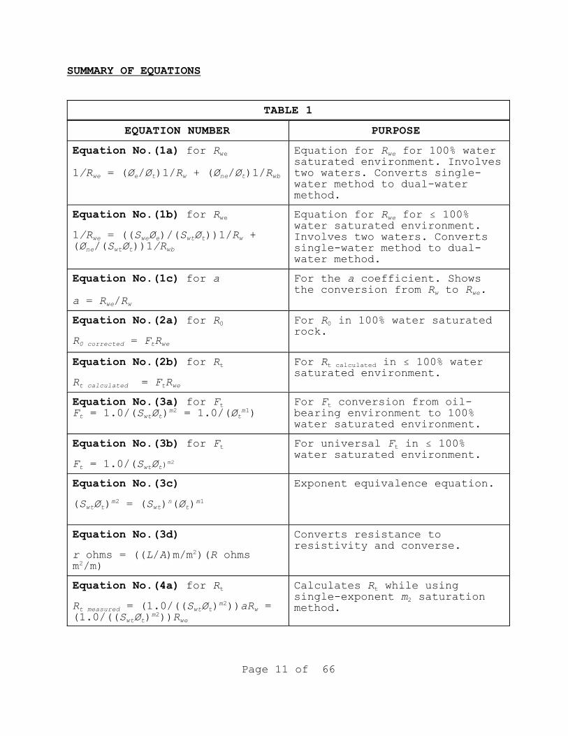
SUMMARY OF EQUATIONS
TABLE 1
EQUATION NUMBER PURPOSE
weEquation No.(1a) for R
we e t w ne t wb1/R = (Ø /Ø )1/R + (Ø /Ø )1/R
weEquation for R for 100% watersaturated environment. Involvestwo waters. Converts single-water method to dual-watermethod.
weEquation No.(1b) for R
we we e wt t w1/R = ((S Ø )/(S Ø ))1/R +ne wt t wb(Ø /(S Ø ))1/R
weEquation for R for # 100%water saturated environment.Involves two waters. Convertssingle-water method to dual-water method.
Equation No.(1c) for a
we wa = R /R
For the a coefficient. Showsw wethe conversion from R to R .
0Equation No.(2a) for R
0 corrected t weR = F R
0For R in 100% water saturatedrock.
tEquation No.(2b) for R
t calculated t weR = F R
t calculatedFor R in # 100% watersaturated environment.
tEquation No.(3a) for F
t wt t tF = 1.0/(S Ø ) = 1.0/(Ø )m2 m1tFor F conversion from oil-
bearing environment to 100%water saturated environment.
tEquation No.(3b) for F
t wt tF = 1.0/(S Ø )m2
tFor universal F in # 100%water saturated environment.
Equation No.(3c)
wt t wt t(S Ø ) = (S ) (Ø )m2 n m1
Exponent equivalence equation.
Equation No.(3d)
r ohms = ((L/A)m/m )(R ohms2
m /m)2
Converts resistance toresistivity and converse.
tEquation No.(4a) for R
t measured wt t wR = (1.0/((S Ø ) ))aR =m2
wt t we(1.0/((S Ø ) ))R m2
tCalculates R while using2single-exponent m saturation
method.
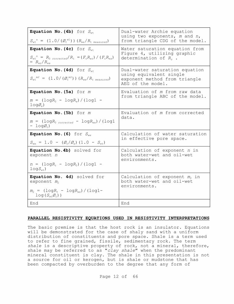
Page 12 of 66
wtEquation No.(4b) for S
wt t we t measuredS = (1.0/(Ø ))(R /R )n m1
Dual-water Archie equationusing two exponents, m and n,from triangle CDG of the model.
wtEquation No.(4c) for S
wt 0 corrected t t wz t waS = R /R =(F R )/(F R )n
wz wa= R /R
Water saturation equation fromFigure 4, utilizing graphic
zdetermination of R .
wtEquation No.(4d) for S
wt t we t measuredS = (1.0/(Ø ))(R /R )m2 m2
Dual-water saturation equationusing equivalent singleexponent method from triangleAEG of the model.
Equation No.(5a) for m
0 wm = (logR - logR )/(log1 -elogØ )
Evaluation of m from raw datafrom triangle ABC of the model.
Equation No.(5b) for m
0 corrected wem = (logR - logR )/(log1t- logØ )
Evaluation of m from correcteddata.
weEquation No.(6) for S
we t e wtS = 1.0 - (Ø /Ø )(1.0 - S )
Calculation of water saturationin effective pore space.
Equation No.4b) solved forexponent n
t 0n = (logR - logR )/(log1 -wtlogS )
Calculation of exponent n inboth water-wet and oil-wetenvironments.
Equation No. 4d) solved for2exponent m
2 t wem = (logR - logR )/(log1- wt t log(S Ø ))
2Calculation of exponent m inboth water-wet and oil-wetenvironments.
End End
PARALLEL RESISTIVITY EQUATIONS USED IN RESISTIVITY INTERPRETATIONS
The basic premise is that the host rock is an insulator. Equationswill be demonstrated for the case of shaly sand with a uniformdistribution of constituents and pore space. Shale is a term usedto refer to fine grained, fissile, sedimentary rock. The termshale is a descriptive property of rock, not a mineral, therefore,shale may be referred to as "clay shale" when the predominantmineral constituent is clay. The shale in this presentation is nota source for oil or kerogen, but is shale or mudstone that hasbeen compacted by overburden to the degree that any form of

Page 13 of 66
porosity has become noneffective, and migrating oil cannot or hasnot penetrated the void space.
The term “connate”, con-nate, often misused and ill-defined inpetrophysics literature and glossaries, is from the Latin meaning:together at birth. In petrophysics it means together at time ofdeposition. Connate water is water entrapped within the pores orspaces between the grains or particles of rock minerals, muds, andclays at the time of their deposition. The water is derived fromsea water, meteoric water, or ground surface water. Otherinvestigators have shown that as clay shales and mudstones arecompacted, a fresh water component of the original connate wateris expelled and an ion-concentrated component remains in thevoids. Therefore, water saturation in the voids remains 100% andw neS is 1.0 in Ø .
The relationship in Eq.(1a) below, presented in Ransom (1977), wasdeveloped to show that conductivity in water-filled voids in thehost rock and the conductivity in clay shale can be represented byparallel conductivity relationships commonly used in basicphysics. The relationship applies to heterogeneous rocks with auniform distribution of minerals and porosity. In resistivity andconductivity relationships the dimensional units for a reservoirbed (m/m ) must be made to be unity so that bed dimensions will2
not be a factor.
For shaly sand it was shown that
we e t w ne t wb 1/R = (Ø /Ø )1/R + (Ø /Ø )1/R (1a)
t e newhere Ø = Ø + Ø .
For 100% water-bearing rock the conductivity relationship inw neEq.(1a) yields 1/R (in clean rock) where Ø is 0.0, and yields
we ne1/R (in shaly sands) when conductive clay is present and Ø isgreater than 0.0.
It should be noted that in this equation there are no limitationswon the resistivity values of formation water R and bound water in
wbshale, R . However, nature does set limits. The bound waterwbresistivity R in the mudstone and clay shale is related to the
original connate water. Waters entrapped at the time of depositiondo vary, but usually do not vary greatly from shale to shale. Seawater has an average salinity of about 35,000 ppm, other surfacewaters probably are significantly lower. However, as indicatedabove, the ion concentration in clay-bound water can increase asfresh water is expelled from the clays with increasing depth andcompaction.
wUnlike connate water, interstitial-water resistivity R in thereservoir can vary over a wide range. Interstitial water mighthave undergone many changes through the dissolution and/or

Page 14 of 66
precipitation of minerals throughout geologic history. It can varyfrom supersaturated salt solutions to very fresh potable waters.Waters in the Salina dolomite (Silurian) in Michigan have specificgravities of 1.458 and a reported salinity of 642,798 ppm. Inother formations, the waters vary to as little as a few hundred
w wb weparts per million. Most often R will be greater than R ; and R ,w wb wa mixture of R and R , will be lower than R . But, it is quite
w wb wecommon for R to have a lower value than R , in which case R willwhave some value greater than R .
In water-filled dirty sands, Eq.(1a) applies. In clean sands, Eq.(1a) becomes
we e t w w 1/R = (Ø /Ø )1/R = 1/R
0and the corrected R in either event is
0 corrected t we R = F R ...(2a)
where, from Figure 1
t wt t t F = 1.0/(S Ø ) = 1.0/(Ø ) ...(3a)m2 m1
0 corrected wt t t wtFor the value of R the value of S Ø becomes Ø because S2 1has become equal to 1.0. Therefore, the exponent m becomes m astdescribed above and in Figure 1. In Eq.(3a), the F that formerly
wt t tpertained to S Ø now pertains only to Ø .
However, in the presence of oil or gas, water saturations arelower than 1.0 and the conductive water-filled volumes are reducedby the displacement of water volume by the hydrocarbon, andEq.(1a) becomes
we we e wt t w ne wt t wb 1/R = ((S Ø )/(S Ø ))1/R + (Ø /(S Ø ))1/R ...(1b)
t calculated t weand R = F R ...(2b)
wewhere R is determined from Eq.(1b), and
t wt t F = 1.0/(S Ø ) ...(3b)m2
wt 2Here S is less than 1.0 and exponent m again becomes m . And, itwill be shown in APPENDIX(B)(3) that
wt t wt t (S Ø ) = (S ) (Ø ) ...(3c)m2 n m1
As it will be seen later Eq.(3b) is the key in the development ofdual-water dual-porosity interpretations. Equation(3b)is a directprogression from the model in Figure 1 and will be furthercorroborated in the development from the common electricalresistance equation, Eq.(3d), that will be developed later.

Page 15 of 66
weNow that the importance of R in the above equations has beenwe westablished, just what is R and can waters represented by R and
wbR actually be combined as seen in Eq.(1b)?
wWater with resistivity R is interstitial water. Water withweresistivity R is not interstitial water and does not exist in
0 corrected 0nature at 100% water saturation, i.e. as R . Resistivity Rcorrected is a hypothetical water mixture of dual waters, influencedby the presence of oil, that exists at 100% water saturation onlyin a dual-water concept. In electrical equations the dual waterscan be mixed together, physically and in nature they cannot. A
wedual-water mixture with resistivity R cannot be recovered in aproduction test.
To continue, a very similar relationship to Eq.(2b), involvingEqs.(1b) and (3b),is seen in work published by Best et al (1980)and by Schlumberger (1989).
[An historical retrospection: Equations(1b) and (3b) resultfrom early developments in resistivity well-loginterpretation. Equation(1a) above was shown in Ransom(1977), and in the presence of hydrocarbon becomes Eq.(1b).The model in Figure 1 in this paper was first seen anddescribed in Figure 2 on page 7 of Ransom (1974). From that
tmodel, F in Eq.(3b) above was first developed. Formationt 3factor F of Eq.(3b) was shown as F in the explanation of
Figure 2, page 7, of Ransom (1974). The equivalencewt t wt trelationship,(S Ø ) = (S ) (Ø ) , is helpful for the use ofm2 n m1
Eq.(3b) in the determination of Archie’s dual-watersaturation. Although the proof of the equivalence is found inAPPENDIX(B)(3) in this paper, the equivalence was first seenas Equation(8)on page 7 of Ransom (1974). Archie’s saturationequation of 1942 was first derived in Ransom (1974)on pages 7and 8. Also, dual porosity was suggested in Ransom (1974),
ewhere Ø was described as hydrodynamically effective porositytand total porosity, Ø , was described as electrically
effective porosity. The difference between the two isnehydrodynamically noneffective porosity, Ø . It was shown how
to calculate all three porosities in Ransom (1977). Archie’srelationships of 1942 were derived in Figure 2 of Ransom(1974), again in Ransom (1995), and again, in considerablygreater detail, in Figure 1 in this paper.
All equations referred to and all equations appearing in thispaper support the fundamental certainty of the influence ofthe geometry of the bulk volume of water on the electricalresistance of rock. The bulk volume geometry concept wasfirst introduced relative to resistivity analysis in Ransom(1974). This concept is best exemplified by the bulk volume
wt tof water term, S Ø , in Eqs.(1b) and (3b), and by water2 1geometry represented by exponent m , and therefore by both m
and n, observed in Figure 1 and seen in Eq.(3b).]
Page 16 of 66
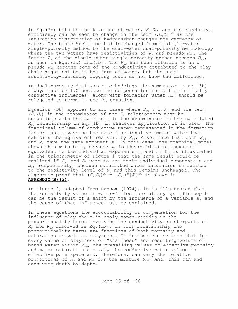
wt tIn Eq.(3b) both the bulk volume of water, S Ø , and its electricalwt tefficiency can be seen to change in the term (S Ø ) as them2
saturation distribution of hydrocarbon changes the geometry ofwater. The basic Archie method is changed from a single-watersingle-porosity method to the dual-water dual-porosity methodology
w wbwhere the two waters have resistivities of R and pseudo R . Thew weformer R of the single-water single-porosity method becomes R ,
wbas seen in Eqs.(1a) and(1b). The R has been referred to as awbpseudo R because some of the conductivity attributed to the clay
shale might not be in the form of water, but the usualresistivity-measuring logging tools do not know the difference.
In dual-porosity dual-water methodology the numerator in Eq.(3b)always must be 1.0 because the compensation for all electrically
wconductive influences, along with formation water R , should bewerelegated to terms in the R equation.
wtEquation (3b) applies to all cases where S # 1.0, and the termwt t t(S Ø ) in the denominator of the F relationship must be
compatible with the same term in the denominator in the calculatedweR relationship in Eq.(1b) in whatever application it is used. Thefractional volume of conductive water represented in the formationfactor must always be the same fractional volume of water that
we wtexhibits the equivalent resistivity R . Also, note that both Stand Ø have the same exponent m. In this case, the graphical model
2 2shows this m to be m because m is the combination exponent1equivalent to the individual exponents m and n. It is illustrated
in the trigonometry of Figure 1 that the same result would bewt trealized if S and Ø were to use their individual exponents n and
1m , respectively, because calculated water saturation is relatedtto the resistivity level of R and this remains unchanged. The
wt t wt talgebraic proof that (S Ø ) = (S ) (Ø ) is shown inm2 n m1
APPENDIX(B)(3).
In Figure 2, adapted from Ransom (1974), it is illustrated thatthe resistivity value of water-filled rock at any specific depthcan be the result of a shift by the influence of a variable a, andthe cause of that influence must be explained.
In these equations the accountability or compensation for theinfluence of clay shale in shaly sands resides in theproportionality terms involving the conductivity counterparts ofw wbR and R observed in Eq.(1b). In this relationship theproportionality terms are functions of both porosity andsaturation as well as clayiness. It further can be seen that forevery value of clayiness or “shaliness” and resulting volume of
nebound water within Ø , the prevailing values of effective porosityand water saturation can vary the conductive water volume ineffective pore space and, therefore, can vary the relative
w wb weproportions of R and R for the mixture R . And, this can anddoes vary depth by depth.
Page 17 of 66
wIt is further illustrated in Figure 2 that as R is corrected towe 0 0 correctedR , R is corrected to R , both by the same factor a. Just
e tas Ø and Ø are two intrinsic properties of the rock and existw wesimultaneously, R and R exist simultaneously and relate to the
same exponent m. The m exponent describes an intrinsic property ofthe rock and produces the parallelism seen in the Figure 2. As aresult, the slope represented by m is independent of the
wconductivity of the waters in the pores. In this figure, R iswerelated to R by the factor a, or coefficient a, that varies depth
weby depth. As a consequence, when these relationships for R areimplemented, or their derivatives or equivalent relationships areused in any resistivity-based interpretation, it is important torecognize that the accountability or compensation by the acoefficient must be removed from the modified FormationResistivity Factor. And, the numerator of the FormationResistivity Factor must always be equal to 1.0 to preventduplication in the accountability for the secondary conductivityprovided by clay shale or other conductive constituents. Thisperspective will be discussed in detail below.
WHAT IS THE FORMATION RESISTIVITY FACTOR
The Formation Resistivity Factor, F, is an intrinsic property of aporous insulating medium, related to the degree of efficiency orinefficiency for the electrolyte-filled paths to conductelectrical current through the medium. The formation factorpertains to and is intrinsic to the insulating medium only. It isindependent of the electrical conductivity of the electrolyte inits pores. Any recognizable, valid extraneous electricalconductivity that sometimes is seen to influence the value of theformation factor must be relegated to appropriate conductivityequations, such as Eq.(1a) and Eq.(1b), where conductivities canbe accommodated by discrete terms.
An equation that demonstrates the purpose of the formation factoris the very basic resistance equation that converts resistivity toresistance:
r ohms = ((L/A)m/m )(R ohms m /m) ...(3d)2 2
where r is resistance, L is length, A is the cross-sectional areaof a straight electrically-conductive path of length L, and R isthe familiar resistivity. The term L/A in the equation is similarto a formation factor and describes a fractional volume havinglength L and cross-sectional area A that is 100 percent occupiedby a single, homogeneous, electrically-conductive medium, eitheran electrolyte or solid. This equation represents 100% efficiencyin the conversion from resistivity to resistance, and theconverse.
Figure 3 is similar to a figure used earlier by Ransom (1984,
Page 18 of 66
1995). This figure represents a unit volume of insulating solidmatter where each side of the cube has a length L equal to 1.0meter. Remove 0.20 of the insulating cube from the center and fill
wthe void with water of resistivity R . Electrical current now canpass from top to bottom of the cube through the water withoutdeviation or interference. This form of electrical path throughthe insulating matter has the highest efficiency.
A measurable resistance implies a measurable resistivity, andresistivity implies conductivity. And, within this insulatingcube, the only electrical conductivity occurs in the fraction thatis water. Therefore, the measured resistance across the examplecube is due to the resistance of the water. Eq.(3d) now can bewritten
cube water w r = (r ohms) = ((L/0.2L )m/m )(R ohms m /m)2 2 2
If this cube were a unit volume of rock where all void volume wasrepresented by 20% porosity, then, the relationship would be
rock water w w r = R = (L/0.2L )(R ) = (1.0/0.2L)(R ) 2
The dimensional analysis of this relationship is
(ohms) = (m/m )(ohms m /m) = (ohms)2 2
and the apparent formation factor is (1.0/0.2L) with units ofreciprocal meters, (m ). After dividing both sides of the equation-1
by the volume represented by L/A, as observed in Eq.(3d),resistance becomes resistivity and the relationship becomes
rock rock t w (A/L)r = R = R = (A/L)(1.0/0.2L)(R )
Here, the dimensional analysis is
(m /m)(ohms) = (m /m)(1/m)(ohms m /m)2 2 2
(ohms m /m) = (m /m )(ohms m /m) = (ohms m /m) 2 2 2 2 2
and the formation factor now is dimensionless and has become
t t F = 1.0/(0.2) = 1.0/Ø = 1.0/Ø m in its simplest form, where exponent m = 1.0.
In addition to showing the relationship between the formationfactor and the void space in the rock, this exercise demonstrates
1that the absolute minimum value for exponent m or m is 1.0 at thehighest possible electrical-path efficiency of 100%.
Theoretically, this degree of efficiency can be duplicated by thepresence of an open fracture or other similar water-filled voidaligned favorably with the electrical-survey current flow.

Page 19 of 66
Although the value of m might never reach 1.0 in practice, thepresence of fractures and similar voids can and do reduce thevalue of m.
There is a fine distinction between the formation factor that isan intrinsic property of rock related to the shape of its voids,and the formation factor that is related to the shape of the waterthat occupies the voids. The intrinsic formation factor isdirectly related to the solid insulating framework of rock and howit shapes the electrically-conductive water volume when watersaturation is 100%, and nothing else. This by definition isintrinsic. But, the size and shape of the conductive water volumealso is influenced by the presence of insulating fluids, such asoil and gas, that can displace water and occupy part of that porevolume. Therefore, the distinction is made that the actual
tformation factor, that will be called F , used in calculations andwtderivations, will involve the term S . At any saturation other
tthan 100%, F no longer is intrinsic.
To carry this demonstration one step further, in the same rocktwhere F = 1.0/Ø at 100% efficiency, if part of the rock is
electrically inert, heterogeneous, porous, insulating rockframework, with a uniform distribution of constituents andporosity, and the remainder is formation water partly displaced by
t wt thydrocarbon, then the former volume of water Ø now becomes S Øwt tand F now becomes 1.0/(S Ø ) for all values of water saturation
wt tand porosity. The fraction S Ø now has become the fractionalcross-section of area in Figure 3 for all electrically-conductivewater paths where the electrical efficiency is 100%.
Not all water-filled electrically-effective pore paths are 100%efficient because the network of interstitial water within therock framework can take on many different shapes andconfigurations imposed by the many and varied properties of the
wt tpore walls and rock framework. Where S Ø is the fractional cross-section area for all electrically-conductive water paths at their
wt thighest efficiency, as in a bundle of straight tubes, (S Ø ) ism2
an equivalent cross-sectional area resulting from all factors thatimpede the flow of electrical current or increase the resistance-to-flow through the rock. This interference to electrical-currentflow is reflected in the steepness of the slopes of the tangential
2 1 wt texponents m , m , and n in Figure 1. As a result, 1.0/(S Ø )wt tbecomes 1.0/(S Ø ) to accommodate the varied geometries of poresm2
and paths for all conditions of pore path inefficiency andinterference, and the Formation Resistivity Factor once againbecomes
t wt t F = 1.0/(S Ø ) from (3b) m2
the same as it was derived from the trigonometrics in triangle AEGof Figure 1.
Page 20 of 66
The Formation Resistivity Factor is aptly named. Resistance r oftthe interstitial-water network, and therefore resistivity R of
the rock, is a function of the size and geometric dimensions ofconfiguration and shape imparted to the water volume within thenetwork of interconnected pores. In one unit of total volume, sizeor cross-sectional area through which electrical current must flowis related to both porosity and water saturation as a fraction ofthat one unit area. Tortuous length, configuration, saturationdistributions, and shape of the electrical pathway filled with
wt twater volume S Ø determine the efficiency or inefficiency of in-place water to conduct electrical current and, therefore, provide
2a value for exponent m .
In this conversion of formation water resistivity to pathwaywt tresistance, the greatest efficiency at any given value of S Ø
1 2occurs when exponent m or m equals 1.0 and m approaches 1.0. And,the greatest effectiveness in one unit of total volume occurs when
wt t tboth S and Ø are 100% or 1.0. When that happens, F = 1.0 and rw= R = R . At any given saturation, overall efficiency of water
t 1 2paths decreases as Ø decreases and/or as m , m or n increases.
All factors that influence the parameters referred to in thisdiscussion determine the efficiency for electrical-survey currentto flow through the rock. These factors, through Archie’sparameters, ultimately determine the value given to the FormationResistivity Factor. Next, we look at those factors.
THE m EXPONENTS
The porosity exponent m is an intrinsic property of the rockrelated to the geometry of the electrically-conductive waternetwork imposed by the pore walls or surfaces of solid insulatingmaterials. This has been verified by investigators of porous mediain extremely meticulous and controlled laboratory investigations,particularly by Atkins and Smith (1961). All minerals havecharacteristic crystalline or particle shapes, whether theminerals are electrically conductive or not, and contribute to thegeometry of the electrically conductive water residing in thepores through shape, physical dimensions of the pores and porethroats, tortuosity, configuration, continuity, pore isolation,orientation, irregularity, surface roughness, angularity,sphericity, and anisotropy. In addition, allogenic minerals, andauthigenic mineral growths such as quartz or calcite or dolomiteor clays, all, contribute to the water geometry within the pores.And, the electrical pathways through the insulating rock areconfigured further by secondary porosity in all its shapes andforms, such as: dissolution porosity, replacement porosity,fissures, fractures, micro-cracks, and vugs in their variousorientations within the rock. Exponent m is related to all thesefeatures acting separately or in concert through the various

Page 21 of 66
inefficiencies (or efficiencies as the case might be) imparted tothe electrically-conductive paths by the diversified voidgeometries, and this results in variations in electrolyte-filledpath resistance and consequent rock resistivity. The greater isthe electrical inefficiency of the shape of the resulting watervolume, the greater will be the value of exponent m, and the
0 tgreater will be R and/or R . This, too, can be seen in Figure 1.
Heterogeneous solid matter, if it is electrically inert,constitutes part of the framework of the rock only and has noother effect on resistivity other than by occupying a position inthe rock framework and possibly displacing interstitial water andinfluencing the pore shape and pore geometry.
Heterogeneous electrically-conductive minerals such as pyrite andsiderite present a different scenario. Their presence not only canaffect the shape of the conductive water paths in the same manneras electrically inert minerals, but can provide electricalconductance in solid matter, not related to pore geometry, thatcan influence rock resistivity. The electrical conductivity ofsuch minerals must be accommodated through the a coefficient inproportionality relationships in Eq.(1a) and (1b), or anequivalent.
In practice, the m exponent usually has a default value of about12.0. In the laboratory, the minimum value for m (or m ) in
homogeneous granular media has been determined to be about 1.3 forspherical grains regardless of uniformity of grain size or packing(Atkins and Smith, 1961; Fricke, 1931; Pirson,1947; Wyllie andGregory, 1952). It was shown in the development of the formationfactor, above, and in Ransom (1984, 1995),that m will decrease inthe presence of an open fracture, dissolution porosity, or fissurewhere the continuous void space is aligned favorably with thesurvey-current flow; and it was further demonstrated that m has anabsolute minimum value of 1.0 at 100% efficiency.
1In the concept in this paper, the porosity exponent m can beestimated from rock containing 100% water by
0 w e m = (logR - logR )/(log1 - logØ ) (5a)
0 corrected we tand m = (logR - logR )/(log1 - logØ ) (5b)
weThe R in Eq.(5b) is from Eq.(1b) and reflects the change inw wbrelative proportions of R and R as they are altered by the
occupation of oil or gas. Although the slope m is intrinsic andthe m from Eqs.(5a) and (5b) should be the same, it is slope mfrom Eq.(5b) that is seen in Figure 2.
1Additionally, a value for m can be determined that applies to alarger range of data. Turn to Figure 5. This figure is a plot of

Page 22 of 66
wa t tR vs Clayiness. The assumption is made that Ø , R , and Clayinesswa tare reliable. The value R is determined by dividing R by the
formation factor in Eq.(3a). In interactive computer methods, theplot is entered by assuming a reasonable value for the m exponent.Select an interval that is believed to contain some wet zones, if
wzpossible. Most often an R trend can be recognized in this plot,w wbas seen in Figure 5. Both an R and R often emerge. If an
windependent R value is known from a reliable source, convert thatwR to the in situ temperature of the logging tool environment at
wthe depth of interest. If the R from the plot differs from thewknown value, iterate by program subroutine between the known R
wand the derived R by incrementally changing m in Eq.(3a) untilthe two values agree. The value of m determined in this manner is
w wbcompatible with the log data for evaluation of R and R .
In the event that the m of Eq.(5a) does not agree with m inEq.(5b), other methods for singular values of m are based onFigure 2. One method is based on the solution of m in similar
wtriangles, and another is based on the dual salinities of R andweR in a method similar to the laboratory method proposed byWorthington (2004). Both methods require considerable iteration inthe evaluation of unknown variables in their respective equations.
It should be noted that on a log-log plot for either measured or0 0 tcorrected values of R (or C ) versus Ø , as in Figure 2, values of
m sometimes can be derived for each specific set of log data orwe 0 correctedrock sample. Individual values of R and R will continually
change with changing clay shale content and water saturation. As aresult, a reliable trend specific to comparable rock samples might
ne tnot be observed for m unless the ratio of Ø /Ø , or otherappropriate discriminator, is held nearly constant to ensure a
w wbnearly constant relationship between the proportions of R and Ras porosity changes. And, laboratory measurements for m must showrepeatability in both m and the resistivity of the influent andeffluent after significant time lapses to prove that themeasurement process, or sample degradation, does not influence thevalue of the measurement being made.
In the single-exponent method for determination of watersaturation, it was seen in triangle AEG that:
2 t we wt t m = (logR - logR )/(log1 - log(S Ø )
2The value of the bulk volume water exponent m is not an intrinsicproperty of rock, as exponent m. It is a hybrid value due to thepresence of oil or gas.
HOW IS EXPONENT n RELATED TO EXPONENT m
The saturation exponent n is the most misunderstood parameter in

Page 23 of 66
formation resistivity interpretation. But, its purpose inelectrical resistivity interpretation is quite straightforward, asis the purpose of exponent m. The saturation exponent n is relatedto both pore geometry and the interference to electrical currentflow within the complex water-filled paths remaining in the poresafter displacement by hydrocarbon has taken place. In Figure 1 andEq.(3b) it is shown that n is a geometrical element similar to m.In Figure 1, it can be seen that slope n is what slope m becomesafter hydrocarbon has migrated into the pores and has displaced afraction of the water.
Historically, and in the absence of better information, the usualdefault value for n in water-wet- and oil-wet rocks has been the
1same as for m (n = m), i.e. exponent m . Also, see discussion inAPPENDIX(B)(4). It has been cited in petrophysics literature thatn often is < m. However, the presence of insulating oil at anysaturation displaces some water volume and produces someelectrical interference and, therefore, the value of n must begreater than m and must decrease the electrical effectiveness ofthe remaining bulk volume of water. The presence of oil cannotincrease the electrical conductivity of water to a value more than100%, and can neither increase the volume of electricallyconductive water paths nor increase the effectiveness of theelectrically effective water paths more than actually exists. Muchto the contrary. Because of increased electrical interference bythe presence of hydrocarbon, the result will be to increase theminimum value of n to some value higher than the value of m, all
1other things remaining the same. Because n is what m has becomeafter hydrocarbon has occupied a fraction of the pore space,
1exponent n cannot have a lower value than the actual value of m .A detailed explanation appears in APPENDIX(D), based on Figure 6,why the actual value of n cannot be lower than the actual value of1m in the same sample, in situ or in the laboratory. Exponent n
1can and will increase over m in the presence of oil or gas as thepresence of hydrocarbon decreases the volume of electricallyconductive water and changes the dimensions of electrical paths,or otherwise impedes the flow of the electrical-survey current.
2Additionally, there can be multiple values for both m and n asoil saturation changes and/or wettability to oil changes. For oil-wet and partially oil-wet rocks this effect can be quitesignificant. When oil is present, in partially oil-wet and oil-wetrocks, for any given water saturation the saturation exponent ncan vary from as low as m to as high as 9.0 or more depending onthe degree of and effectiveness of wettability to oil, physicaldistributions of oil and water, oil properties, and rock-frameworksurface properties and characteristics. In Figure 1,it can be seen
tthat at any constant value of R , if the redistribution of aconstant fraction of oil causes the electrical interference to
2change, then exponent n (and m ) will change, and this will resultwtin a corresponding change in the value of S .

Page 24 of 66
The exaggerated influence due to the presence of oil will increasewt 2both the usual exponent n for S and the combination exponent m
wt tfor bulk volume water S Ø . For any given porosity and any given2oil saturation, the slopes for exponents n and m will increase
with those properties of the rock and pore walls that when coveredwith adhesive oil films increase the interference to the flow ofelectrical current through the conductive paths. These factorsincrease in severity with the increase in wettability to oil,finer grained sandstone (increased surface area), increasedefficiency of packing, increased number of grain-to-graincontacts, finer pores and pore throats, properties of oil(increase in viscosity of oil), interfacial tension betweenoilfield brine and crude oil, isolation of pores, and the physicalsaturation distributions of both the wetting- and nonwetting-phases whether oil or water. All these influences act in concertat their respective levels of severity to cause or alterinterference to electrical current flow.
In oil-wet and partially oil-wet rock, the effects of thesefactors become magnified and the electrical interference withinthe pore paths is increased. As a result, the saturation exponents
2n and m increase. In oil-wet rock, it might be thought that thehigher the value of these exponents, the higher will be the oilsaturation. To emphasize, that is not the case. Figure 1 showsthat the saturation exponent n represented by slope CG of triangle
0 corrected tCDG is the resistivity gradient employed between R and R relative to changes in the saturation of oil (or water).
2 we tSimilarly, exponent m is the gradient between R and R relativewt tto changes in bulk volume water, S Ø .
The maximum value for n in any specific water-wet rock is thatvalue where the presence of oil or gas has the greatesteffectiveness in producing electrical interference. This occurs athigh water saturations. Interference and how effective thatinterference can be are not the same thing. The effectiveness ofthe interference to increase resistivity is greatest at higherwater saturations, and is least effective to increase resistivityat low water saturations. Read that carefully. Observe theeffectiveness curves in Figure 10. The greatest electricalinterference occurs in rock with the greatest wettability to oiland depends on the distribution of the oil and its viscosity. Theminimum value for n occurs where the interference caused by thepresence of hydrocarbon exhibits the least effectiveness inproducing electrical interference. The greater the value of n or2m for any given value of resistivity, the greater will be thecalculated water saturation. But, these statements should notimply that there is a strong relationship between the value of n
2or m and the value of either water or oil saturation. There isnone. That is because of the many different factors that caninfluence the presence and distribution of oil and its properties,
tand thereby influence R . There is no mathematical relationship
Page 25 of 66
2between the value of exponents n or m and the value of oilsaturation, except when within the same bed with uniformelectrically effective constituents. To the contrary, it will beseen later in this paper, and can be seen in Figure 1, that if allother things remain constant, as exponent n increases along angle
2ã (or ä) or m increases along angle â, water saturation increaseswith the possibility of increased water cut; and/or, water production takes place without significant oil. In the model, it
t 2can be seen that when R is constant, if n or m increases, the2slope representing n or m becomes more vertical (n might increase
to 8 or 9) and the downward projection of slope n is towardwt 2increased water saturation, S , and the downward projection of m
wt tis to an increased bulk volume of water, S Ø .
That having been said, it must be understood that the two2exponents n and m not only represent gradients, but represent
efficiency or effectiveness. And, effectiveness of oil tointerfere with the flow of electrical survey current is greatestat high water saturations where oil saturation is the lowest. Thisis corroborated by the slope CG representing exponent n in Figure1. Is this contrary to anything said above? It might appear so,but in actuality, it is not.
These features relative to the presence of oil, and sometimes gas,must be recognized. Is there any exception? Theoretically, itmight be possible to hypothecate a condition whereby the value ofn could have a value lower than m, but it is not likely. Inliterature, the value of exponent n with a value lower than m iscommonplace and overwhelmingly is accepted as conventional wisdom;but, it violates physics and it has never been explained in thesame literature how a valid n < m can occur. In the laboratory n <m is a common occurrence due to sample damage or degradation. Insitu, n < m would be a violation of physics.
See discussion under APPENDIX(D). For a comprehensive treatment ofn, please study the explanations under OBSERVATIONS ANDCONCLUSIONS FROM FIGURE 10 ABOUT EXPONENT n. The discussionsfollowing the Observations and Conclusions absolutely corroboratetriangle CDG of the model in Figure 1.
Gas usually does not have the same exaggerated effect on n as oilunless the reservoir has been filled with oil at some former timein geologic history and an adhesive film of remnant oil precedesthe occupation by gas. The resistivity of a gas-bearing zone canincrease, however, due to the decrease in irreducible watersaturation. This, too, can be demonstrated in Figure 1. Theprimary exaggeration in n is with partially oil-wet and oil-wetrocks that are filled with oil or have been filled with oil at aformer time whether as a reservoir or as a migration path.

Page 26 of 66
THE a COEFFICIENT
Historically, the a coefficient always has appeared in thenumerator of the modified Formation Resistivity Factor, and hasbeen perpetuated in industry with no defined purpose. In thismodel there is no support for the appearance of an a with aconstant value in the formation factor. The formation factor isintrinsic to the rock at 100% water saturation. The a coefficientis not an intrinsic property, but is dependent on variables notrelated to the electrically inert rock or to the physicalgeometries of its pores. The a is related neither to volume norshape imparted to the network of electrically-conductive waterpaths. The a coefficient contributes nothing to alter efficiencyof the conversion of water resistivity to resistance, or viceversa. In the model, the shift in resistivity corresponding to aalways is found in the resistivity axis, and the shift varies fromdata to data with depth. Coefficient a emerges as an inherent andinseparable factor of the complex resistivity relationship, as inEqs.(1a) and (1b), and is related to the proportions of allsecondary electrically-conductive constituents and influences that
w wbvary the relative proportions of R and R .
weIt can be seen in the graphics of Figure 2 that R is the productw w we weof a and R , therefore aR = R . R varies from depth to depth,
and so does coefficient a. It can be seen in this relationshipthat a varying a coefficient technically can be used in single-
wewater single-porosity methods where R is not calculated. But, inwedual-water dual-porosity methods where R is calculated, the a
coefficient cannot be used as an independent parameter. If the ais used in single-water single-porosity methods, it must becalculated properly. And that is difficult to do when the correctvalue of a varies with rock constituents and depth, and only onewater and one porosity is available to work with. That is one ofthe reasons why dual-water dual-porosity methods were conceived.
wWhen a is associated with R , as in the equation developments ofw(1a) and (1b), and as a multiplier or reduction factor for R , the
a coefficient more readily can be recognized as being anindispensable factor that accounts for those heterogeneities thatproduce additional electrical conductivity. Coefficient a is the
wcomposite factor that relates R to the resistivity value of thew wbcombination of R and R , and all other natural electrically-
weconductive influences, in such proportions to result in R .
In the modified formation factor used in single-water single-porosity methods, the a coefficient appeared in the numerator. In
wthe modified formation factor the a became a multiplier of the Rwin Archie’s saturation equation. The aR became a single-water
wesingle-porosity equivalent to R .
Secondary conductive influences, inherent to the rock, that
Page 27 of 66
produce coefficient a can be: clay shale, surface conductance, orsolid semi-conductors such as pyrite and siderite as separateinfluences or in concert. One influence that is neitherelectrically conductive nor intrinsic is hydrocarbon saturation.These in turn, and perhaps others, can produce a change in rockresistivity.
The occurrence of one additional electrically-conductive influencewould add one more term to Eqs.(1a) and (1b), or their equivalent,
wt tand if there were no change in S Ø , the value of the compoundcoefficient a would be reduced. These influences, all, can changew weR to an apparent or pseudo value R with a corresponding change
0 0 correctedin R to R at their respective porosities.
Technically, in dual-water dual-porosity methods, the coefficienta should be transposed from the modified Formation ResistivityFactor term to the water resistivity relationship. For example:
0 corrected t we t w t w t we R = F R = (a/(Ø ))R = (1.0/(Ø ))aR = (1.0/(Ø ))R m m m
The question might be asked, "What is the difference?" There area number of reasons, four of which are:
1. The a coefficient is a required proportionality factor,related to all factors influencing the electrical conductivity of
w wethe rock, that convert resistivity R to R , and is calculatedwealong with R at each depth increment.
2. To prevent duplication by the user in the correction forweconductive influences. Duplication occurs when both a and R
appear in the same water-saturation equation, or when a appears asan independent variable in dual-water dual-porosity methods. Anysaturation relationship involving resistivity can employ either
wecoefficient a or R , but not both. 3. To prevent the use of a constant artificial and unwarrantedcorrection factor.
4. Although the formation factor is meaningless at 100%tporosity, the value of F always must be 1.0 when both porosity
tand water saturation in the F equation are 1.0.
As explained above, and in Figure 2,
we w a = R /R (1c)
After substituting Eq.(1c) into Eq.(1b), a relationship is derivedshowing the proportionality terms in coefficient a for the usualshaly sand:
we e wt t ne wt t w wb 1/a = (S Ø )/(S Ø ) + (Ø /(S Ø ))(R /R )

Page 28 of 66
It can be seen here that coefficient a is a function of watersaturation as well as porosities. See APPENDIX(A) for furtherexplanation. This is the evaluation for the a coefficientappearing in Figure 2.
This relationship is shown for comparison purposes or informativepurposes only. It is not to be calculated and used independentlyin dual-water dual-porosity methods because it already has been
weincorporated in the calculation of R as can be seen in Eq.(1b).
THE SATURATION EVALUATION
tThe model in Figure 1 is a diagram showing that R is a functionwt tof both the volume of water S Ø and the inefficiency with which
electrical current passes through that water. The inefficiency ofthe electrical current flow is related to the distribution of thewater and the interference to that flow within the water networkas it is reflected in the exponents m and n of the expression
wt t wt(S ) (Ø ) . In the model it is shown that logS is the length ofn m
tthe projection along the X-axis between logØ and the intercept oftslope n with logR . This length also is represented by length CG
of triangle CDG in Figure 1.
Revisiting Eq.(1b), (2b), and (3b), the reader already might havededuced that water saturations can be estimated from theseequations. Keeping faithful to the self-evident truth that thevolume of water referred to in the denominator of the formationfactor must be the same volume of water that provides electrical
weconductivity in the R equation, then Eq.(1b) can be used onlywe wtwith Eq.(3b). Therefore, when S (or S ) is less than 100%, the
product resulting from Eq.(1b) and (3b) is
t calculated t we R = F R same as (2b)
t wt twhere F = 1.0/(S Ø ) from (3b)m2
After combining Eq.(2b)and (3b) when either the measured or actualt tR is substituted for the calculated R , then
t measured wt t w wt t we R = (1.0/((S Ø ) ))aR = (1.0/((S Ø ) ))R ...(4a)m2 m2
However, it was illustrated in Figure 1 in triangle ACG, and inwt t wt tAPPENDIX(B)(3), that (S Ø ) is equivalent to (S ) (Ø ) ,as seenm2 n m1
in the equivalence equation (3c) therefore Eq. (4a) resolves to
wt t we t measured S = (1.0/(Ø ))(R /R ) ...(4b)n m1
Archie’s dual-water dual-porosity equation.
It was passed over quickly that Equation (4a) also yields Archie’s

Page 29 of 66
equivalent single exponent version seen here
wt t we t measured S = (1.0/(Ø ))(R /R ) ...(4d)m2 m2
weOnly one R equation can be used in this calculation. It will bewt 0from Eq.(1a) or from Eq.(1b). At S = 1.0, the calculations for R
are the same in either equation if the water mixture is the same.wt tAt S < 1.0 only Eq.(1b) should be used for calculating R because
weit is the only equation that allows the calculated R to reflectw wbthe changing proportions of R and R resulting from the
displacement of interstitial water volume by oil or gas. InEq.(1a) the proportions of the two waters are fixed by the mineralconstituents of the rock. But, the relative proportions of the twowaters and their electrical efficiencies also change with thechange in saturation and distribution of oil and gas, and these
0 correctedchange depth by depth. The R must be determined from thesame water mixture proportions and water geometry that exist at
teach R measurement. These proportions are reflected only in theconductivities shown in Eq.(1b). The efficiencies are reflected in
t tthe exponent residing in F , and the F used must be compatiblewith each variation in water saturation, and that is Eq.(3b).
For Eq.(4b), Eq.(1b)can be simplified after the substitution forwe eS Ø has been made from the volumetric material balance equationfor water,
wt t we e ne S Ø = S Ø + (1.0)Ø .
After the substitution, Eq.(1b) becomes
we w ne wt t wb w 1/R = 1/R + (Ø /(S Ø ))(1/R - 1/R ) simplified Eq.(1b)
weThis version of R is used in Eq.(4b).
t measuredThe R in Eq.(4b) must be corrected for environmentalconditions and tool-measurement characteristics before watersaturation is calculated.
wtThe term S in the formation-factor relationship of Eq.(3b) is thekey element in the dual-water dual-porosity relationship. The termwtS is an inherent part of the formation factor derived from the model in Figure 1.
It can be seen in Eqs.(1b) and (4a) that the a coefficient isvariable with depth and mineralization and is included as part ofwe weR . When R has been calculated, and is used, the appearance of aconstant a coefficient in the formation factor, usually as afraction less than 1.0, would be gratuitous and would artificiallyincrease the calculated hydrocarbon saturation in productive andnonproductive zones alike; and, in this model, would be bothlogically and mathematically incorrect.

Page 30 of 66
Figure 1, together with Figure 2, is a concept model that hassignificant informative and educational value. The graphics of themodel are meant primarily to illustrate, to develop, or to explainwhat is calculated blindly by algebraics in computer-programsubroutines.
In an interactive computer program, irreducible water saturation orother core-derived information can be input for the purposes ofexamining the plausibility, validity, and integrity of certainparameters. On a well log above the transition zone in oil-bearingreservoir rock, for example, tthe intersection of R with alaboratory value of irreducible water saturation fixes the upperlimiting value of saturation exponent n for that specific set ofdata. However, when irreducible water saturation is known, thisupper limit of exponent n should be calculated from the algebraicsof Eq.(4b), or Eq.(4c) as will be shown below. The same can be saidfor the lower limit of n in the same rock which could be estimatedby inserting water saturation when oil saturation is irreducible.
1But, in either exercise, no value of n can be lower than m . Thetactual value of R is required for each of these procedures,
whether derived from the well-log or rock sample.
The water saturation equation, Eq.(4b), has been developed from thetrigonometric model in Figure 1 and again corroborated by thealgebraic development of Eq.(4b), all, for certain heterogeneous,but uniform, environments. And, each development herein shows thatit authenticates Archie's basic relationships presented in 1942,and further refines these relationships in the developments anddiscussions.
It has been said that Archie's relationships are empiricaldevelopments. Whether or not this is true, it has been shown herethat Archie's classic relationships and parameters have amathematical basis, and have forthright and substantive relevanceto rock properties that is quite different from many acceptedtheories and usages in industry literature.
Saturation exponent n is the most difficult of all the parametersto evaluate. If a valid value of oil saturation is known, or can bederived, the value of exponent n can be estimated by substitutionin Eq.(4b) or (4c). When the actual values of m and n are known, orcan be derived, either or both can be important mappableparameters, and a mathematical relationship between m and n notonly can be an important mappable parameter, but can be a possibleindicator to the degree of wettability to oil or distribution ofoil under in situ conditions. This information not only can beimportant in resistivity log analysis but can be important in thedesign of recovery operations.
The calculation of Eq.(1b) is required in the solution of the waterwtsaturation relationship in Eq.(4b). Because water saturation S

Page 31 of 66
wealso appears in the proportionality terms within the R equation,wtEq.(1b), an algebraic solution for S in Eq.(4b) is not viable and
is not considered. Probably the simplest and best method for allanticipated integer and non-integer values of n is an iterativesolution performed by a computer-program subroutine. Graphicallythe iteration process can be demonstrated by a system ofcoordinates where both sides of Eq.(4b) are plotted versus input
wt wtvalues of S . As S is varied, the individual curves for the leftwtand right sides of Eq.(4b) will converge and cross at the S value
that will satisfy the equation.
Figure 4 shows a crossplot of example data to demonstrate theequivalence of the graphical solution to the iterations performedby a computer-program subroutine. The following input values arefor illustration purposes only.
w m = 2.17 R = 0.30 wb n = 2.92 R = 0.08
t t Ø = 0.22 R = 20.00 ne Ø = 0.09
In Figure 4 it can be observed that when values from each side ofwtEq.(4b) are plotted versus S the two curves have a common value at
a water saturation of about 0.485. The iteration by subroutine willwtproduce the same S of about 0.485 or 48.5% for the same basic
input data.
It is worthy of note that in the volumetric material balance forwe e wt twater, when S Ø goes to zero the absolute minimum value for S Ø
nein this example is 0.09, the value of Ø . The mathematical minimumwtwater saturation S that can exist in this hypothetical reservoir
ne t wbis Ø /Ø = 0.4091 or 40.91% where R becomes 0.08. The minimumsaturation of 40.91% is related only to the pseudo bound water inclay shale and tells us nothing about irreducible water saturationin the effective porosity. If this were an actual case in a water-wet sand, at 48.5% water saturation, water-free oil might beproduced because the only water in the effective pore space mightbe irreducible. Grain size and surface area would be aconsideration. Any water saturation below 40.91% cannot exist andis imaginary.
wt weFor the conversion of S to S , either the material balance forwater (shown above) or the material balance for hydrocarbon(Ransom, 1995), can be used. In terms of hydrocarbon fractions, thematerial balance for the amount of hydrocarbon in one unit volumeof rock is
wt t we e (1.0 - S )Ø = (1.0 - S )Ø
weFor the calculation of S the balance can be re-arranged to read:
we t e wt S = 1.0 - (Ø /Ø )(1.0 - S ) ...(6)
Page 32 of 66
weand S now can be estimated.
When the material balance equation for hydrocarbon is multiplied bythe true vertical thickness of the hydrocarbon-bearing layer,either side of this equation produces the volume of hydrocarbon perunit area at in situ conditions of temperature and pressure.
we wt w wbFinally, for the evaluation of R , and S in turn, both R and Rw wbmust be known. In the event neither R nor R is known, these
values most often can be estimated by interactive computer graphicswa wafrom a crossplot of R (or C ) versus Clayiness (% clay) as shown
in Figure 5, from Ransom(1995), where clayiness is estimated bywaappropriate clay-shale indicators. R is determined by dividing the
t t t wt t tcorrected value of R by F where F = 1.0/(S Ø ) and F hasm2
t wtresolved to 1.0/(Ø ) because S always must be 1.0 for them1
w wb 1determination of R and R . The value for exponent m should be thesame value of m that will be used for the final interpretation. The
tvalue of R may be taken from wireline tools or measured whiletdrilling. As pointed out earlier, the measured R should be
corrected for environmental conditions and measuring-toolwacharacteristics. In a figure such as Figure 5, R values from zones
known to be or believed to be 100% water-filled often describe awztrend or curve identified as an R trend where hydrocarbon
saturation is zero. This trend can take virtually any curvature,steep, convex, concave, or flat, depending on the layering and
w wbisotropical resistivity relationship between R and R . If the clayminerals within the reservoir bed are detrital, they almost alwayswill have similar electrical properties to the surrounding clayshales. However, the clays found within a reservoir bed can bedifferent from the clays surrounding the bed, particularly if theclays within the bed are authigenic, i.e. detrital minerals thathave dissolved and re-formed in place as pore-lining crystals. Ifthe difference in electrical properties is measurable, a dog-legcan appear in the described trend. The trend, however, is importantfor saturation analysis only throughout the reservoir beds. It isimportant that the electrical behavior and clay-indicator behavior
wzof clays be consistent and repeatable. Once the R trend has beenestablished within the reservoir beds it can be extrapolated to 0%
w wbclay for R , and extrapolated to 100% clay for R at in situw wb wzconditions. These values of R , R , and R have been estimated from
preliminary formation factor and clay indicator information and aresubject to examination by the analyst.
wz wbAlthough, in Figure 5, the end point of the R trend for R is saidto be defined at 100% clayiness, 100% clayiness might not exist forthe formation. But, when Figure 5 is used as a reconnaissance tool,it is not important to know the actual amount of clay present forthe estimation of water saturations. The X-axis could be renamedClay Index for this work. The relationships in the vertical axiswill not change if the scale on the X-axis is changed. It isimportant, however, that the clayiness measurement methods and

Page 33 of 66
resulting clayiness estimations be consistent and repeatable.
w wbThe values of R and R determined from Figure 5 can be used intEq.(1b) because they are compatible with the corrected R from
which they came. These values are compatible because they have beenderived by the same method from measurements by the sameresistivity measuring device at the same environmental conditionsof temperature, pressure, and invasion profile at the same momentin time.
wz we wHowever, the R values, or simulated R values, found between Rwband R are similar to those calculated from Eq.(1a). Be that as it
we wtmay, Eq.(1b) becomes Eq.(1a) when S = S = 1.0 at all points alongwz wethe R trend. The instant that oil or gas becomes present, S and
wtS become less than 1.0, and Eq.(1a) becomes Eq.(1b). Hydrocarbonwsaturations decrease the volume of water with resistivity R , and
weinfluence R by making its value move closer to the resistivitywb wevalue of R . See Figure 2. If R were to plot, it would produce a
wzdeparture in the vertical axis from the R trend, either higher orwb wlower depending on whether R is higher or lower than R . But, it
wewill not plot as R from Eq.(1b) because it does not exist innature at 100% water saturation, so there can be no natural data.we wa we wtR from Eq.(1b) becomes another R the instant S and S become
weless than 1.0. The R of Eq.(1b) exists only in mathematical formwithin a dual-water concept. If there is a significant difference
w wbbetween the end-point values of R and R the difference betweenwz wethe R and the calculated R increases. See APPENDIX(A) for further
explanation.
It is interesting to note, however, that from Figure 5 alone, oncewz wean acceptable R trend has been established, that generalizes R ,
estimated water saturation can be previewed by
wt 0 corrected t t wz t wa wz wa S = R /R =(F R )/(F R ) = R /R (4c)n
wtIt can be seen here that the previewed value of S can ben
w wbestimated independently of porosity, m, even R and R , all interms of an estimated input value for clayiness at each specificdepth. The value of exponent n lies between its minimum value of m,corrected or as established above, and its maximum value determinedfrom irreducible water saturation. Furthermore, unlike the more
wtrigorous Eq.(4b), once exponent n has been established, S can bepreviewed or estimated directly from Eq.(4c). A cautionary noteappears in APPENDIX(C).
Figure 5 has other uses than as a preview of water saturations inshaly sands. Figure 5 can be used as a reconnaissance tool topredict the abundance of organic matter or total organic carbon, orthe occurrence of oil- or gas-deposits in shales and marlstones forfurther analysis. Also, it can be used as a means for selectingdepths for taking additional measurements on available cuttings

Page 34 of 66
samples. It is one of the purposes of this plot to direct attentionto zones of special interest for further investigation.
CHALLENGING WELL-LOG EXAMPLES
This part will address two vintage well log examples, chosenbecause of their uniqueness and simplicity. All well bores in allwell examples have been drilled with a fresh-water-based mud asverified by the SP curves. Figure 7 illustrates an oil-bearing bedin Well 1. Figure 8 illustrates the same oil-bearing bed in Well 2.It is not known which well was drilled first. There is noinformation about the reservoir beds in either example other thanWell 1 produced much water and very little or no oil in aproduction test(s). The question is: Why does the bed in Well 1 notproduce oil? Observe Figure 7 and Figure 8 during the followingdiscussions.
Figure 7, Description of Well 1. This well has a significantresistive marker at the depth of 2516. The zone of interest is ZoneA that lies between the depths of 2545 and 2620. This zone doescontain oil. Zone A was tested over the marked intervals in thedepth column and produced a large quantity of water and little tono oil. This bed, Zone A, exhibits a very distinctive annulusproving that there is both movable oil and movable water in theradial zone disturbed by invading drilling-mud filtrate. The deep
tresistivity curve suggests that R is 100 ohm-meters or greater andtransitions to the predominantly water-bearing Zone B that lies
tbetween 2620 and 2629. In the predominantly water-bearing zone, R0appears to be around 14 ohm-meters. Could this be R ? No other
information is available. The question is: Why did a productiontest on Zone A recover a large amount of water from an apparentlyviable oil-bearing zone?
FIGURE 8, Description of Well 2. This well example is from the samestratum as Well 1 above. This well has the same marker as in Well 1above, at 2536. The zone of interest is Zone A that lies betweenthe depths of 2562 and 2596. This zone also contains oil. The SPcurrents are responding to the interference due to the presence ofoil. In contrast to Well 1, Zone A in Well 2 does not exhibit an
tannulus. Why? The deep resistivity curve suggests R is around 100ohm-meters and the bed transitions to Zone B that lies between 2596and 2631 that appears to be wet with a resistivity of about 10 ohm-meters. Zone B transitions again to zone C that lies between 2631and 2639 that appears to be even wetter with a resistivity of about4 ohm-meters. Zone A at the upper part of this bed appears tocontain oil. This bed in Well 2 provides more information than theequivalent bed in Well 1, however, the question still remains: Whywas the large amount of water produced from what appears to be aviable oil-producing zone?
Channeling of water from the water-bearing zones B or C is not

Page 35 of 66
expected to be the answer, although it is a remote, but unlikely,possibility. But, it will be seen that there is another, moreplausible possibility.
Information Derived from Logs from Wells 1 and 2: The calibrationof the well logs on these two wells probably is not perfect, andthere probably are inconsistencies between the two wells.
In Figure 7, Well 1, the gamma ray tool is very sensitive and showssome statistical variation. Zone A between 2545 and 2620 exhibits avery-well-developed annulus. The presence of an annulus means thatthere is both movable oil and movable water within the radial zonedisturbed by invading drilling-mud filtrate. The radius of mud-filtrate invasion is shallow. The radius of invasion and resulting
tdisturbance ends at the leading edge of the annulus. The R forthis bed probably is in excess of 100 ohm-meters. The presence ofmobile oil does not mean that the oil can be produced. It doesmean, however, that the bed is very porous and permeable. With noother information to guide us, it might appear that Zone B between
02620 and 2629 is nearly 100% water saturated. If so, then R wouldt 0be about 13 ohm-meters. The ratio of R /R of resistivity in the
upper zone to that in the lower zone is about 10:1 and surelymerits further investigation. The upper zone was tested over thedepth intervals marked in the depth track and much water wasrecovered along with an insignificant amount of oil.
In Figure 8, Well 2, the zone of interest is Zone A between 2562and 2596. The interesting thing in this zone is that there is noannulus. The hydrostatic pressure is great and mud-filtrate spurt-loss invades porous and permeable rock immediately as the drill bitpenetrates the rock. Impermeable mud cake cannot develop on theface of the rock until the drill bit passes by and leaves the faceof the rock open. An annulus then develops along with the creationof a filter cake that soon becomes an impermeable membrane, butbegins to dissipate when the mud-filtrate no longer can invade therock. Well 1 probably was logged with the resistivity toolimmediately after drilling-mud circulation ceased and drill pipewas retrieved from the bore hole. The well, therefore, was loggedwhile the annulus was still visible. After the mud circulationstopped and drill pipe was withdrawn from Well 2, the welloperation probably incurred some delay before logging began. Duringthat lull the annulus had time to dissipate before the well waslogged. This behavior is not unique. Examples of this behavior havebeen observed by the author in “before” and “after” well loggingsessions on numerous occasions, and are described in Ransom (1995).The dissipation of the annulus by the diffusion process is commonin high-porosity, highly permeable reservoir beds, particularlywhere relative permeability to water is high compared with that tooil. In Zone A in Well 2, with the dissipation of the annulus andinvaded zone, all resistivity curves read nearly the same and all
tare believed to approximate R . Has this zone and the upper zone inWell 1 been recently depleted and only oil at residual saturation
Page 36 of 66
remains? Why do these zones have such high resistivity and stillproduce only water?
A second zone in Well 2, Zone B, appears between 2596 and 2631. Theradius of invasion is deeper in this zone than in Zone A because alesser amount of oil is present and the relative permeability towater is higher. This zone has a resistivity of about 10 ohm-
0meters. This resistivity is not R because there is another zonebelow from 2631 to 2639 that shows even a lower resistivity. Thisbottom zone (Zone C) has a resistivity of about 4 ohm-meters and
0probably is R for both of the reservoir beds shown in Wells 1 and2. If so, this makes the occurrence of all the water in theproduction tests that much more puzzling. Have the interesting topzones A in each well been depleted by recent emigration and nowexhibit only residual oil? Then, what about Zone B between 2596 and2631 in Well 2? This zone probably exhibits remnant oil after oilmigrated out of the bed by natural means over geological time. Thiszone corresponds to Zone B between 2620 and 2629 in Well 1.
A depth marker in Well 1 appears at 2516. This marker could becompared with the correlative marker 2536 in Well 2 to helpdetermine the depth relationship of one bed relative to the otherand might help to explain any migration. But, the elevation of thedepth datum is not known in either well so the true depthrelationship between the A Zones cannot be determined. It remainsthat a quasi interpretation must be made in an effort to explainwhy neither zone of interest produces oil.
Deductive Interpretation: The potential oil-bearing beds in Wells 1and 2 are found at shallow depths. Both porosity and effectivepermeability to water are expected to be high because of the lackof compactive overburden at the shallow depths of the beds ofinterest. This is supplemented with the reality that large amountsof water was recovered in the production test(s).
A second reason that the rock is thought to be very porous andhighly permeable is because of the complete dissipation bydiffusion of drilling-mud-filtrate in Zone A of Well 2. Theporosity of Zone A in each well is expected to be higher than 25%,perhaps as high as 30%. Porosity of the bed and relativepermeability to water are high and relative permeability to oil islow in this reservoir bed. Because of the expected good quality ofthe rock, the value of exponent m is believed to be low.
0Resistivity R can be taken from zone C in Well 2, and is believedtto be about 4 ohm-meters. Resistivity R in Zone A in Well 1 is in
excess of 100 ohm-meters and in Well 2 is approximately 100 ohm-meters. It is possible that the difference in calibration betweenthe two logging tools would account for some of the difference int weR values, but the more likely reason is the differences in R and
newater-filled Ø .

Page 37 of 66
It is believed that oil might be at residual saturation in eachZone A, by emigration or by prior production from nearby wells. Butwhat is the residual oil saturation value? It is not known, butcould be 20%, 30%, 40%, 50%, maybe more.
t neThe assumptions for any further calculations are: Ø = 0.30, Ø =0.05, and m = 1.6. It should be noted that experienced analystswill agree that these assumptions are most favorable for thecalculation and prediction of oil production.
wThe calculated R from zone C in Well 2 is about: 0.58
Questions inspired by these wells are:
a) Should the prominent oil-bearing bed in either well beproduction tested?
b) Should casing be set in either well?
c) Is water channeling to the test depth from a location lower in the bed?
d) Should attempts be made to isolate the tested depth interval in Well 1 and re-test?
e) Should Zone A in Well 2 be tested?
f) Can the water saturation be estimated?
Questions elicited here can be addressed with a certain amount ofcaution:
a) To be absolutely certain that primary oil production is notviable, Well 1 probably should have been tested, as it was, butwith the expectation that no oil would be recovered.
b) No oil can be produced by primary production methods in eitherZone A. No casing should be set in either well, unless enhanced oilrecovery methods are entertained. Any method of recovery that candecrease the viscosity of the oil should be considered. If theviscosity of oil in Zone A can be reduced, whatever oil would beproduced would have a very high water cut and the operatorproducing such oil would have to be prepared to handle the waterproduced.
c) Water is not channeling from a lower level to Zones A or B ineither well.
d) No attempt should be made to isolate the test interval in Well 1and re-test.
e) Zone A in Well 2 should not be tested.

Page 38 of 66
f) What is the residual oil saturation in Zone A or B in eitherwell? Because of the high resistivity and ample thickness in bothZones A, it is possible that enhanced oil recovery methods could besuccessful, but might not be economical. If considered viable andemployed, perforations should be set high in the bed and withdrawalrate should be low to minimize coning by water. But, as it will beshown below, only the maximum calculated oil saturation can bepredicted from these well logs and Figure 10. The actual oilsaturation in any zone is speculative. It cannot be determined fromthese resistivity well logs alone. Other well logs and/or otherdisciplines should be employed.
tA general conclusion is the reservoir bed is oil-wet because R inZones A for both Well 1 and Well 2 have such high values in a rockwhere the assumed porosity is so high. Such resistivity values fortR are 100 ohm-meters or more in the suspected oil-bearing zone
0(and can be much higher in other oil-wet rocks) but the probable Ris only about 4 ohm-meters.
The relative permeability to water is much higher than the relativepermeability to oil. This is corroborated by the large amount ofwater recovered in production tests.
Because the relative permeability to water and that to oil isw wsignificantly different, and because the mobility of water (k /ì )
o ois greater than the mobility of oil (k /ì ) an annulus can form inZone A of Well 1. Because the mobility of water is high, the timerequired for an annulus to develop or to dissipate is short as itwas proposed for Well 2
The reason why large amounts of water along with virtually no oilwas produced during production test(s) in Zone A, Well 1, isbelieved to be because the mobility (k/ì) of water is so high andthe mobility of oil is so low.
Because of the logic immediately above, the oil is expected to bevery viscous, and the presence of oil is likely to reside atresidual saturations in Zones A and B in both wells.
Because the proposed residual oil saturations in Zones B are lowerthan the oil saturations in Zones A, it is believed that the oiloriginally in place in both Zones B has been reduced by naturalemigration over geologic time.
OBSERVATIONS AND CONCLUSIONS FROM FIGURE 10 ABOUT EXPONENT n
Examine the curves drawn in Figure 10.
All calculations of exponent n shown in Figure 10 are based ontriangle CDG of the model in Figure 1. Triangle CDG is the graphic

Page 39 of 66
depiction of the dual-water Archie two-exponent water saturation Eq.(4b).
The values of the calculated n from the logic of triangle CDG inthe model and from Eq.(4b) are summarized in the type curves drawnin Figure 10.
How to Interpret Figure 10. Caution. Do not think of the curves in Figure 10 as profiles.
Each type curve represents a relationship between exponent n andwtsaturation S in a specific reservoir bed or same sample of rock at
a deep radial depth beyond the invaded zone.
Imagine each of the curves as a series of smoothed bar graphs forexponent n over a full range of water saturations at a constant
tvalue of R . At any specific water saturation, the n value at thatwater saturation represents the degree of, or the effectiveness of,the interference by oil to the flow of electrical survey current inoil-wet- or water-wet rocks.
Not all of the chart is applicable. The values of exponent n aremeaningful only at oil saturations greater than irreducible oilsaturation. The values of n can be calculated in the region of
tirreducible oil and in the flushed zone only if the appropriate Ris known and employed.
tThe curves are applicable only where a constant value of R remainsvalid. The curves are not valid where water saturations are high
tand exponent n is steep because a high value of R cannot besupported at high water saturations. At high values of watersaturation, exponent n will begin a decline and continue to declineas water saturations increase until it reaches the value of
texponent m. In Figure 1, resistivity R also will decline along0with the decline of n until it reaches the value of R .
As a result, the steep upward mathematical sweep of n valuesprobably does not exist in nature. The high values of n can be
tcalculated, but at high values of water saturation R must0ultimately return to R , thus n will return to m.
One of the first things to be observed in Figure 10 is that in bothZones A and B in Wells 1 and 2, as the resistivity gradientdescribed by exponent n increases, predicted water saturationincreases and the predicted oil saturation decreases. And, wherethe oil saturation is the greatest, exponent n is the lowest.Puzzling? This is in precise conformity with the prediction byexponent n illustrated by slope CG of triangle CDG in Figure 1.
For example:

Page 40 of 66
1. If the voids in the rock are filled to a high oil saturation, anincrease of 10% oil will decrease the volume of electricallyconductive water correspondingly. 2. If the voids in the rock are filled to a low oil saturation, anincrease of 10% oil will displace the same bulk volume of water asat high saturations.
3. Wherever the oil phase is continuous, whether at low saturationsor high saturations, the electrical interference caused by adhesiveinsulating oil films on the pore surfaces will be nearly the same.
4. Although the electrical interference by oil in items 1 through3, immediately above, is the same wherever the oil exists in acontinuous phase, Figure 10 and the model in Figure 1 illustratethat the effectiveness is not the same.
5. The effectiveness of the interference by oil is greater athigher water saturations than at lower water saturations as seen bythe increased values of n. This phenomenon is corroborated by themodel in Figure 1, Equation (4b), and the type curves in Figure 10.
In Figure 10 what do the curve crossovers mean at point H? Figure10 illustrates that everywhere oil is present, the true value ofexponent n is greater than exponent m, but some calculated valuesof n are lower than m. Why?
The calculated oil saturation is highest where exponent napproaches exponent m. In both Figure 1 and Figure 10 that maximumcalculated oil saturation level is seen at point H. In Zones A inWells 1 and 2, that maximum occurs at about 90% oil saturation(disregarding irreducible water saturation) where the curves forZones A meet the assumed value of 1.6 for exponent m.
In Figure 10, because the n curves for Well 1 Zone A and Well 2Zone A, intercept the value of m at high oil saturations, it wouldimply that there is more oil to be produced from this reservoir.For Zone B, the highest oil saturation that can be calculated isabout 50% where the curves for zones B also meet the value ofexponent m at a point H. This behavior is illustrated in Figure 1where line CG (slope n) of triangle CDG collapses to line CH thatrepresents slope m. Any calculated value of n lower than the valueof m is imaginary.
What about the imaginary values of n in Figure 10? The oilsaturation where the calculated n crosses the value of exponent mat location H represents the highest oil saturation that can becalculated for that data and that well depth. It does not implythat the specific saturation at H is the predicted saturation forwater or oil. Examine the model in Figure 1. Remember: Exponent mbecomes exponent n after some of the interstitial water has been

Page 41 of 66
displaced by oil. So, in Figure 1 when gradient CG collapses alongangle ä to lie on gradient m (now n = m) it cannot collapse anyfurther. The maximum oil saturation is predicted by the
tintersection of the extrapolated slope of m and the level of Rwherever intersection H resides. This is the same H as appears onthe effectiveness chart in Figure 10. The calculated values of nlying below the value of m do not exist. The imaginary valuesabsolutely can be calculated, but cannot be reproduced in thelaboratory or in nature. Such values published in petrophysicsliterature are disputable. The model exhibited in Figure 1representing the dual-porosity Archie Equation, Eq.(4b), ismathematics, but the slope CG collapsing to the limiting value ofthe extended slope m is physics.
Exponent n is higher in Zone A than in Zone B at the same watersaturation in both wells. It can be seen in Figure 10 there is no
wtmathematical relationship between exponent n and S observedbetween one bed and another at any constant saturation value.
tAs R changes, the slope representing values for n might or mightnot change. Exponent n can vary independently of water saturation.For the value of n to increase above that of m, it is necessaryonly for oil to be present. Water saturation influences n, but,except for coincidences, there is no curvilinear relationship
wtbetween S and n except within the same bed, and the bed exhibitsuniform distributions of oil, water, porosity, and other factorsinfluencing electrical conductivity, as the individual curves inFigure 10 illustrate.
What if the imaginary values are used in interpretation? Slope m in0Figure 1 is a resistivity gradient representing the value of R at
100% electrical efficiency in the selected rock at all porosities.tIf slope n were to lie below slope m, resistivity R would lie
0below the extrapolated values of R , and oil saturations would beartificially overestimated over all porosities and saturations.This is a commonplace occurrence in literature that has become afactoid of conventional wisdom. The presence of oil cannot increasethe electrical conductivity of water more than 100% efficiency (m).See Figure 6 and APPENDIX(D).
Figure 9. Description of Well 3. This well log, too, is a vintageresistivity log. This log was chosen because of its simplicity. Inthis figure is a resistivity log in a water-wet rock. Like the twoexamples above, the resistivity curves show great contrast between anoil-bearing zone and a water-bearing zone. This example shows a dualinduction log with an SP curve. At the top of the bed between X151 andX161 is an oil-bearing interval marked Zone A. Near the bottom of thebed is a water-bearing interval between X183 and X192 marked Zone B.
The calculated values of n relative to water saturations for this bedalso are shown as a curve in Figure 10.

Page 42 of 66
A moderately high value of saturation exponent n up to perhaps 8 or9 might not be a factor in distinguishing between water-wet and oil-wet rocks.
As it can be seen in Figure 10, as water saturation in Well 3increases, the calculated curve for n will increase again the same asthe curves for Wells 1 and 2. This, again, is corroborated by theslope CG representing exponent n of triangle CDG in the model inFigure 1.
Examine the effectiveness curve from Zone A of Well 3 in Figure 10.This curve is plotted from values of exponent n in water-wet rock. Itcan be seen that the curve is very similar to the curves from oil-wetrock. Why is this so?
It is a simple matter for a computer to solve the necessary equationsand iterations required to compute the results appearing in Figure10. Let’s examine how exponent n is calculated:
weIn the calculation of each exponent n, R first must be calculatedwt wefrom Equation(1b) for each iterated value of S . Along with R ,
exponent n must be solved from triangle CDG in Figure 1 or from thedual-water Archie equation, Eq.(4b):
wt t we t measured 0 t measuredS = (1.0/(Ø ))(R /R ) = (R /R ) (4b)n m1
where from triangle CDG of Figure 1,
t 0 wt 0 t wtn = (logR - logR )/(log1 - logS ) = (logR - logR )/(logS )
0 t measuredIt can be seen in Eq.(4b) above, that the ratio (R /R ) varieslittle for each Zone A in the Wells 1, 2, and 3. Therefore, theequation for each curve in Figure 10 is:
wtS = a near constant for each depth of interest depending on then
value of the ratio.
wtSolve for n by iterating S in Eqs.(1b) and (4b).
Can oil-wet zones be distinguished from water-wet zones by highvalues of n? Sometimes and sometimes not. In Well 1, Zone A, an oil-
0 t measuredwet zone, the ratio of (R /R ) is approximately 10/100 = 1/10 oreven smaller. In Well 2, Zone A, also an oil-wet zone, the ratio
0again is approximately 10/100 = 1/10 or thereabout (smaller if R istaken directly from Zone C). And in Well 3, Zone A, a water-wet zone,the ratio is about 1/10. So, it doesn’t matter whether the zone isoil wet or water wet the calculated values of n in these cases can benearly the same for the same water saturations. When Equation(4b) issolved for exponent n it can be seen in these ratios that there islittle difference in Equation (4b) whether the rock is oil wet orwater wet. Although, at high n values, the rock probably is oil wet,

Page 43 of 66
but it is not always the case.
In some oil-wet rocks, the ratio might be very small. The ratio of0 t measuredR /R might be 10/1,000 or 10/10,000. It can be seen in
t weEquation(4b) that as R increases (or R decreases), exponent n0 tincreases. The ratio R /R in this order of magnitude moves the type
curve shapes upward in Figure 10 because exponent n increasesteverywhere. As R increases, point H on both Figure 1 and Figure 10
will be shifted to the right toward higher calculated maximum oilsaturations.
The values for exponent n are viable only at higher oil saturationsthan irreducible oil saturations. This must be taken intoconsideration. The calculated bulk volume of oil consists ofproducible oil and irreducible oil; and the calculated bulk volume ofwater consists of water that can be produced, irreducible water, andwater, or pseudo water, contained in dynamically non-effective rockconstituents.
What about the steep upward sweep of n at high water saturations?Like the values of n found below the value of exponent m, they tooare imaginary. They can be calculated, as reported above and seen in
tFigure 10. They actually would exist if the specific value of Ractually existed at the high water saturations, but it does not. At
wt thigh values of S the high values of R used in the calculations arenot co-existent, and do not exist in real life. Hence, the upwardsweep in n at these saturations is artificial. The n values areimaginary.
The actual values of n must gradually return to the value of m at highwater saturations so that at 100% water saturation and 0% oilsaturation exponent n becomes m again. From some location on theeffectiveness curve, as water saturation increases, the value of nwill increase to a maximum whereupon, as water saturation continues
tto increase, the value of n declines followed by a decline of R untilt 0the water saturation becomes 100%, n becomes m, and R becomes R .
The dashed curve in Figure 10 is one of a number of artful conceptionsthat exponent n might take as oil migrates into or out of water-wet-
t tor oil-wet rock, simultaneously changing R . As R increases, the0 tratio R /R (in Eq.(4b)) decreases and exponent n increases. As n
increases, the apex becomes narrower and sharper from which n declinesto approach and ultimately return to exponent m at 100% watersaturation.
In Figure 10, the effectiveness curves under these conditions mightresemble normal frequency curves skewed heavily toward high watersaturations, and slope CG in triangle CDG in Figure 1 mightcorrespondingly morph into a shape similar to a lazy S as high watersaturations approach 100%.

Page 44 of 66
Both the model in Figure 1 and the curves in Figure 10 would betmodified as R changes to correspond with the reasoning set forth
above.
2What about exponent m ? This is a single saturation exponentequivalent to the two exponents m and n for saturation calculations.It is derived from triangle AEG in the model in Figure 1. If the
2effectiveness curve for m were shown in the chart in Figure 10, thecurve would lie between the constant exponent value of m and thecurves for n. A close inspection of Figure 1 will show that the slope
2representing m is greater than that of slope m but smaller than thatof slope n. It also can be seen that triangle AEG has its origin atwe 0R instead of R , triangle AEG is more tolerant of errors. Because ofthe greater length between AG over CG, slope AG will change less thanslope DG for the same error in porosity or saturation.
2Everything that has been said about exponent n applies to exponent m ,2with the exception that the effects on or by m will be smaller. On
both Figure 1 and Figure 10, where the slope of exponent n meets the2slope of m at point H, so does the slope of exponent m meet slope m
at point H.
ARE THERE LIMITATIONS TO ARCHIE’S RELATIONSHIPS DEVELOPED IN THISMODEL?
Are there rocks that complicate resistivity interpretations? Ofcourse. As in every discipline and in every analytical method, therecan be problems that complicate the interpretation process. That isnot unique to Archie’s relationships, whether new or old. Above, itwas mentioned that Archie’s relationships, as they have been developedin this paper, apply to heterogeneous rocks with uniform distributionsof porosity, saturations, and electrically-conductive constituents.That is a requirement for all matter subject to electricalinvestigations. Problem rocks are those that exhibit nonuniformdistributions of causative factors that influence resistivity. Suchfactors or conditions can be, but are not limited to: anisotropy, bedsconsiderably thinner than the vertical resolution of the loggingtools, bedding planes at high angles relative to the borehole axis,human error in running the wrong resistivity-measuring tool for theexisting resistivity profile in the mud-filtrate invaded zone, etc.Are these Archie problems? No. These are problems that affect allrelated analytical resistivity methods. These are problems that eithernature or the shortcomings of man have dealt to the analyst. Theseconditions are part of the interpretation process and require theattention of qualified well-log analysts.
CONCLUSIONS
The most important thing to be drawn from this paper is the model in

Page 45 of 66
Figure 1. From that model, two versions of Archie’s saturationequation are derived for dual-water dual-porosity conditions: thecommon two-exponent version and an equivalent single-exponent version.Also, each of Archie’s parameters have been derived, identified, andexplained. These fundamental relationships and parameters have beenderived from trigonometrics of the graphic model and corroboratingalgebraics, and have shown that Archie’s relationships developedherein are a dual-water methodology.
Second. is the definitive exploration of the exponent n illustratingits behavior in both water-wet and oil-wet rocks. This exhaustiveexploration reveals information about the saturation exponent n thatnever before has been revealed in literature.
The concept described herein is based on the very fundamentalelectrical law relative to the conversion of resistance toresistivity, and on the efficiency of the network of pores andpathways in the rock through which the electrical-survey current mustflow. The basic electrical resistance equation is the key tounderstanding the Formation Resistivity Factor. The true formationfactor equation alone contains all terms necessary for the calculationof Dual Water Archie.
Archie’s relationships, as the parameters have been defined in thismodel, have been shown to apply in dual-water dual-porosity conditionsand in shaly sands and other rocks of limited heterogeneity. Themethodology developed herein can serve as the spine to which numerouscorrectional and mineral-specific subroutines can be attached to addanalytical refinements. The model and the foregoing developments inthis paper have shown that Archie’s relationships have astraightforward, physical and mathematical basis, and, in thisconcept, have been shown to apply to heterogeneous rocks with uniformdistributions of porosity, saturations, and electrically-conductiveconstituents.
Archie’s relationships are fundamental and the foregoing developmentsare deemed necessary for the relationships to be understood, used inliterature, and employed in saturation calculations. An understandingof what influences these parameters and what they represent willprovide the user with a place to start and a recognition of what isrequired from other disciplines for the solution of interpretationproblems, and will complement the user’s inventory of tools fordescribing rocks as they reside in nature.
EPILOGUE
A good well-logging interpretation program is like a double-edgedsword. It must cut both ways. The program must find hydrocarbons wherethey exist and must not imply their existence where they do not exist.The purpose is to be accurate with consistent reliability. Together

Page 46 of 66
with interactive computer graphics, the author has used the foregoinglogic and fundamentals as the skeletal framework to guide resistivityinterpretations for many years in all parts of the world.
ACKNOWLEDGMENT
I wish to acknowledge Ben W. Ebenhack, Associate Professor ofPetroleum Engineering at Marietta College and founder of the non-profit AHEAD Energy Corp. Mr. Ebenhack reviewed this paper and offeredsuggestions and encouragement for its publication.
SYMBOLS DEFINED
a Historically, the coefficient of the Formation ResistivitywFactor. In this paper, the coefficient of R . Usually equal to
1.0 in clean rocks, and different from 1.0 in the presence of anyconductive influence other than formation water. Often lower than
we1.0. When incorporated in comprehensive R relationships, thenumerator in the Formation Resistivity Factor must always be 1.0.
m The porosity exponent in the Formation Resistivity Factor. Relatedto the shape and dimensions of electrolyte-filled paths. There
1are two versions of exponent m. One is the usual m (or m ) forthe two-exponent version of Archie’s equation, and the other is2m for the equivalent single-exponent version.
n The saturation exponent found in Archie's water saturationequation. Related to the electrical interference caused by thepresence of hydrocarbon in electrolyte-filled paths. Whatexponent m becomes after hydrocarbon has migrated into the rockand has displaced water.
tØ Total porosity fraction consisting of the sum of effective andnoneffective porosity fractions.
eØ That part of the total porosity fraction that is hydrodynamicallyeffective and can be occupied by hydrocarbon.
neØ Is the noneffective porosity in clay shale related to waterattracted to the clay crystal and water held osmotically, and isdirectly related to the fraction of clay shale present. It is aporosity volume that has not been penetrated by hydrocarbon.Water saturation in the noneffective pore space is 1.0 and
wbresistivity is represented by R .
tF The Formation Resistivity Factor of the rock, where thewt t wtconductive water volume fraction always is S Ø , where S # 1.0.
In this paper, the numerator always is equal to 1.0.

Page 47 of 66
wR Formation water resistivity. Interstitial-water resistivity.
wa tR The apparent resistivity of formation water found by dividing Rt wt 2by F , where S = 1.0 and m = m.
wbR The apparent resistivity of water bound in clay shales.
we weqR Same as R in other work. A calculated value for the equivalentwater resistivity when secondary conductive influences are
wpresent. In this paper, the product of coefficient a and R asweit is incorporated in Equation (1b) for the calculation of R .
wWater with resistivity R is interstitial water. Water withwe weqresistivity R (or R ) is not interstitial water and does not
exist in nature at 100% water saturation. It is a hypotheticalwater mixture of dual waters, influenced by the presence of oil,that exists at 100% water saturation only in a dual-waterconcept. Electrically the dual waters can be mixed, physicallythey cannot. This dual-water mixture cannot be recovered in aproduction test.
wz waR Is the R value determined from a zone known to be or believedto be completely filled with water or nearly saturated with
wzwater. Hydrocarbon saturation is zero or near zero. R is awe wagraphical approximation of R and a special condition of R .
0R The true resistivity of the uninvaded rock when water saturationis 1.0. The water or pseudo water can have the resistivity valueweR . Sometimes calculated, sometimes read directly from the deepresistivity curve, sometimes derived from the deep resistivity
0 tcurve. R is a special condition of R .
tR The true resistivity of the uninvaded rock, whether or not itcontains hydrocarbon. Sometimes read directly from the deepresistivity curve, sometimes derived from the deep resistivity
0 tcurve, sometimes calculated. R is a special condition of R .
we eS Water saturation as a fraction of the effective porosity Ø .
wt tS Water saturation as a fraction of the total porosity Ø .
wt t wtS Ø The total conductive water volume fraction where S # 1.0. Afraction of one unit of formation volume. Sometimes referred toas the bulk volume of water.
REFERENCES
Archie, G. E., 1942, The Electrical Resistivity Log as an Aid inDetermining Some Reservoir Characteristics, Trans., AIME, vol.146.

Page 48 of 66
Atkins, E. R., and Smith, G. H., 1961, The Significance of ParticleShape in Formation Resistivity Factor - Porosity Relationships,Journal of Petroleum Technology, AIME, vol. 13.
Best, D. L., Gardner, J. S., and Dumanoir, J. L., 1980, A computer-processed wellsite log computation, SPE paper 9039, RockyMountain Meeting Proceedings, Society of Petroleum Engineers.
Fricke, H., 1931, The Electric Conductivity and Capacity of DisperseSystems, Physics, August.
Keller, G. V., 1953, Effect of Wettability on the ElectricalResistivity of Sand, Oil and Gas Journal, Jan. 5; 51: 62-65.
Pirson, S. J., 1947, Factors Which Affect True Formation Resistivity,Oil and Gas Journal, November 1.
Ransom, Robert C., 1974, The Bulk Volume Water Concept of ResistivityWell Log Interpretation. A Theory Based on a New Reservoir RockResistivity Model, The Log Analyst, SPWLA (Jan.-Feb.)
Ransom, Robert C., 1977, Methods Based on Density and Neutron Well-Logging Responses to Distinguish Characteristics of ShalySandstone Reservoir Rock, The Log Analyst, SPWLA (May-June)
Ransom, Robert C., 1984, A Contribution to a Better Understanding ofthe Modified Archie Formation-Resistivity-Factor Relationship,The Log Analyst, SPWLA (March-April)
Ransom, Robert C., 1995, Practical Formation Evaluation, John Wiley& Sons, Inc., New York.
Schlumberger, 1989, Log Interpretation Principals/Applications.
Sweeney, S. A. and Jennings, H. Y., 1960, The Electrical Resistivityof Preferentially Water-Wet and Preferentially Oil-Wet CarbonateRocks, Producers Monthly, 24, 29-32.
Worthington, P. F., 2004, Characterization of the Intrinsic PorosityExponent through Dual-salinity Measurements of ElectricalConductivity, Petrophysics, SPWLA, (November-December, pp. 499-516)
Wyllie, M. R. J. and Gregory, A. R.; 1952, Formation Factors ofUnconsolidated Porous Media; Influence of Particle Shape andEffect of Cementation; Paper Number 223-G presented at Fall Meeting of the Petroleum Branch, AIME, held at Houston, TX.,October, 1-3.

Page 49 of 66
APPENDIX
PREFACE. The model appearing in Figure 1 incorporates Figure 2. Theweorigin always is R , the apparent or equivalent resistivity of
we wformation water. But, R is the same as R in clean rocks andwdifferent from R in heterogeneous rocks, and in the presence of
wehydrocarbon saturation. The influence of hydrocarbon saturation on Rcan be observed in Equation (1b) found under PARALLEL RESISTIVITYEQUATIONS USED . . .
tThe Y-axis is R , the resistivity of rock containing water. The X-axiswt t t wtis S Ø , the bulk volume of water, consisting of two parts, Ø and S .
t wtIt must be recognized that Ø and S have no units, but are fractionst wtand in themselves are not volumes. As fractions, neither Ø nor S has
resistivity because neither is dimensional. Only bulk volume water canhave volume and, therefore, can have resistivity. This could beconfusing, because the fraction that is bulk volume water inliterature must be multiplied by a dimensional conversion factor thathas a value of 1.0 and appropriate three-dimensional units. Now beingdimensional, the bulk volume water can have resistivity.
In the discussion of the Y-axis, the basic resistance-resistivityequation must be introduced. That equation is:
water water resistance = (L/A) ◊ resistivity
Dimensionally, ohms = meters/meters ◊ ohm meters /meter2 2
(water) (F) (water)
The expression (L/A) is a formation resistivity factor in its simplestform. It converts resistivity to resistance, and resistance toresistivity. So, how does resistance of water become resistivity ofrock?
0 tIn Figure 1, R and R are resistances of water per unit length, andat the same time resistivities of the unit volume of rock thatcontains that water. In inert, electrically non-conductive rock, wateris contained in the pore spaces of the rock. The water volume occupiespore paths and creates electrically conductive paths that exhibitvarious levels of electrically conductive efficiency. These paths canhave various degrees of resistance as the dimensions of (L/A) arevaried in the resistance-resistivity equation above. However, theresistance of the water over the length of rock in a unit volume ofinsulating rock constitutes the resistivity exhibited by that rock.Numerically, the resistance of water is the same as the resistivityof rock,
In Figure 1, the resistance of water over a unit volume of rock is theresistivity of the rock. The Y-axis in Figure 1 is resistivity of rockexcept at 100% porosity where it is the resistivity of water.

Page 50 of 66
(A) Figure 2. This figure shows the function of coefficient a. In thesection above related to coefficient a an equation was written showingall the variables used in the calculation of a. One of the variableswas water saturation in the effective pore space. Why is thatnecessary?
The presence of hydrocarbon decreases the volume of water in theeffective pore space. This changes the proportionality of water volume
wwith resistivity R relative to the volume of pseudo water withwbresistivity R that is associated with clay shales. In a parallel
we wbconductivity relationship this moves R closer to the value of R ascan be seen in Figure 2.
wInput value R is from the best known source or from Figure 5 afterclayiness has been determined by the best clay indicators available.
e tPorosity values, Ø and Ø , are determined by traditional methods, orfrom Ransom (1977, 1995), after employing the appropriate matrixvalues for the host rock.
wCoefficient a is shown to be a multiplier of R but is nevercalculated independently for use in an interpretation program when it
weis an integral part of R , as seen in Eqs.(1a) and (1b). In dual-waterdual-porosity methods, coefficient a may be calculated only as amatter of interest, but must never appear in a saturation equation
wewith R .
(B) Figure 1. Figure 1 illustrates the model that Archie’srelationships obey. It is intended for informative and illustrativeuse, only. It is not drawn to scale. The inclinations of the straightlines representing slopes are determined by trigonometric tangents.The value of a specific trigonometric tangent is the value of thespecific m or n. The steeper is the slope, the greater is theinterference and resistance to electrical-current flow through thepores and pore paths in the rock, the greater is the inefficiency forthe transmission of electrical-survey current, and the greater willbe the value of m or n.
wt t(1) On the X-axis, it is seen that S Ø decreases to the right. Atstudy of the logarithmic scales will show, for example, that Ø = 0.2
wt wt tand S = 0.3; and, as a result, their product S Ø = 0.06.
(2) There are three right triangles of interest in Figure 1. They aretriangles ABC, CDG, and AEG.
In any triangle shown in the figure, the slope or tangent of an angleis described as the side opposite divided by the side adjacent. Thetrigonometric law pertaining to tangents, that right triangles follow,can be described as:
tangent of acute angle = (side opposite)/(side adjacent)

Page 51 of 66
Because the X-axis is descending in value to the right of the origin,the sign of the tangent will be negative. Therefore, on the log-logplot such as Figure 1,
(tangent of acute angle)(log(side adjacent)) = log(side opposite)
and, 1/(side adjacent) = (side opposite)tangent of acute angle
Trigonometry was created for solving problems. Express thesetrigonometric functions in equation form and the Formation ResistivityFactor and an improved Archie’s water saturation relationship willemerge.
In Figure 1, the tangent of the acute angle â of the right triangleAEG is represented by
2 log tan â = m = (EG)/(log1 - log(AE))
2 t -m (log(AE)) = log(EG) = logF
t F = 1.0/(AE) m2
In equation form, this is
2 t wt t m = logF /(log1 - log(S Ø ))
2 wt t t -m (log(S Ø )) = logF
t wt t F = 1.0/(S Ø ) . . .(3b) m2
In Figure 1, the tangent of the acute angle of the right triangleCDG is represented by tan = n = log(DG)/(log1 - log(CD))
t 0 corrected -n(log(CD)) = log(DG) = (logR - logR )
0 corrected t (CD) = R /R n
In equation form, this is
t 0 corrected wt n = (logR - logR )/(log1 - logS )
wt t 0 corrected -n(logS ) = (logR - logR )
wt 0 corrected t (S ) = R /R . . .(4b)n
wt t wt t(3) (S Ø ) has the same function as and is equal to (S ) (Ø ) .m2 n m1
2 wt t t weIn triangle AEG, -m (log(S Ø )) = logR - logR

Page 52 of 66
wt t we t (S Ø ) = R /Rm2
wt t 0 correctedIn triangle CDG, -n(logS ) = logR - logR
1 t 0 corrected weIn triangle ABC, -m (logØ ) = logR - logR
1adding the two equations that involve n and m , yields
wt 1 t t we -n(logS )+(-m (logØ )) = logR - logR
wt t we t S Ø = R /Rn m1
wt t we tBut, (S Ø ) = R /R , from triangle AEG above.m2
wt t wt tTherefore, (S Ø ) = (S ) (Ø ) . . . same as (3c) m2 n m1
This equivalence also was proved graphically in Eq.(8) on page 7 inRansom (1974).
(4) In addition, in partially oil-wet or oil-wet rocks, the assumptionthat n = m can lead to calculated water saturations that are too low.In Figure 1, it can be seen that when the default value of n equals
tm the line representing n will intercept the R level far to the rightat H. The resulting calculated water saturation can be too low andmight even be “unreasonable”. When the corrected n value is used, the
tslope representing n will intercept the level of R at point Gsomewhere near point H or to the left of H, which will yield a
wt“reasonable” value for S depending on the value of n. Straight lineswtrepresenting values of n can rotate along the arc ä as either n or S
varies. The slopes representing n should intercept the corrected valuetof R at calculated water saturations within the saturation range
between irreducible water and irreducible hydrocarbon.
(5) In oil-wet or partially oil-wet rocks the presence of oil willincrease the interference to the flow of electrical current, causingthe value of the saturation exponent n to increase. In Figure 1, itcan be seen that as the value of the saturation exponent n increases,the slope of n increases. In Figure 1, under the condition that there
twill be no increase in R , as the slope of n increases, thecalculated water saturation will be seen to increase. In oil-wet rock,a film of viscous adhesive oil coats the walls of the pores and porethroats. The value of n is related to the degree of electricalinterference caused by the adhesive oil, and that degree ofinterference can be caused by adhesive oil films whether or not theoil saturation and oil distribution is sufficient for oil productionto take place. Figure 1 shows that the saturation exponent n is the
t 0 corrected tresistivity gradient that R employs between R and R relativeto changes in the saturation distribution of oil, not to the value ofoil saturation. It is related to the value of oil saturation only
tthrough R . The saturation exponent n is not to be confused with thesaturation value of oil. Figure 1 suggests that with no increase in

Page 53 of 66
tR and with varying degrees of effectiveness of the coating of porewalls and pore throats with adhesive,viscous oil, this condition canallow a high water saturation to exist with the result that no oilwill be produced, or oil will be produced with a high water cut. Ifoil is to be produced with a low water cut or with zero water cut thenthe oil must reside in a continuous phase that allows the oil to moveand in such quantity and distribution that it causes discontinuity inthe water phase. If the presence of oil resides in a continuous phasein oil-wet rock, this condition will present further increasedinterference to the flow of electrical survey current with the result
tthat the value of R will increase to uncommonly high resistivitylevels.
It might be inferred from Figure 1 that the ideal condition for oilproduction to take place in oil-wet rocks would be for the value of
tn to be as low as possible and the value of R to be high. Under thistcombination the slope of n will intercept the level of R farther to
the right on the X-axis. Calculated water saturation will be lower andoil might be produced with a reduced water cut or no water cut. Whereare these conditions likely to be found? Examples might be in rockcontaining relatively large, well sorted grains or in rock with wellinterconnected dissolution porosity. These conditions will be foundin good quality reservoir rock where the value of porosity exponentm is low.
wa(C) Figure 5. This figure is a plot of R vs Clayiness (% clay). Itt wacould have been a plot of corrected R vs Clayiness. The plot of R
vs Clayiness yields more information relative to secondaryconstituents. The plot also has uses in focusing attention on data anddepths where unexpected events or mineralization occurs.
When calculating clayiness for this plot, clayiness should bedetermined from the best clay-shale-responsive indicators available,but never from an average of several. Consider the influences on eachof the clay-responsive measuring methods before each is entered intothe clay-estimation process.
(D) Figure 6 is nearly the same as Figure 1. Like Figure 1, Figure 6is not intended to be a working graphical procedure, it has beenexaggerated to illustrate detail, and it is intended only to beinformative and explanatory. In Figure 6 it is shown that the same
wt trock can contain the same volume fraction of water, S Ø , whether ornot oil or gas is present. In Figure 6, the example uses the sameporosity and saturation values as seen depicted in Figure 1. In thisexample, m is uniform throughout the host rock. If water saturationis 100% when the porosity is reduced to 0.06,thenwt tS Ø = 1.0 x 0.06 = 0.06. This is the value of the total water volumeas a fraction at J. The same volume of water can be observed in thesame rock when the porosity is 20%, but oil or gas displaces 70% of
wt tthe water volume: S Ø = 0.30 x 0.20 = 0.06. This is the total waterwt tvolume as a fraction at K. This common value of S Ø is shown at E at

Page 54 of 66
wt tthe base of Figure 6 on the logarithm scale for S Ø . In Figure 6, where the example rock shows a water volume fraction of
00.06, it can be seen that when n < m, R at resistivity level J willtbe greater than R at resistivity level K, for all values of porosity
and all values of saturation. In real life this cannot happen. But,when the value of n is found to be or made to be < m in the samesample of rock, most users will not recognize the impossibility ofthis condition.
When n is said to have a lower value than the host value of m, thet 0associated values of R always becomes less than R at equivalent water
volumes in the same rock. And that associated value is profoundlyt 0incorrect. For R at K to have a lower value than R at J, the
migration of oil or gas into the interstitial water volume must makethe electrical paths through the remaining water volume moreefficient. This enhancement of the electrical conductivity of thewater paths through the interstices by the presence of oil, must bedone with no change in salinity. Hypothetically, for oil or gas tomigrate into the undisturbed effective pore space and cause the valueof n to be < m, the presence of oil or gas must cause the electricallyconductive paths of water to become more efficient. This, the presenceof a continuous phase of oil or gas in water-wet rock cannot do. Inthe model in this paper, which is faithful to laws of physics, whenall other things remain unchanged, it is shown that it is impossible
tfor the actual value of R to have a lower value than the extrapolated0value of R for the same quantity of water in the same sample. But,
can there be an exception to this rule? Probably not. To do so wouldbe in conflict with physics. Any occupation of pore space by oildecreases the electrically conductive volume of water and, therefore,increases the resistivity gradient.
When n < m the slope representing the n becomes so low that fortwhatever value of R exists, the slope representing an aberrant n will
tintercept that level of R far to the right at an artificially lowwater saturation value on the right-facing Figures 1 and 6. Theconsequence is that the calculated water saturation will be too lowand the hydrocarbon saturation will be over estimated indiscriminatelyin producible and non-producible hydrocarbon-bearing beds alike. Thiswill be an insidious by-product that most users will not anticipate.
To accept a value for n that is lower than m, is to deny that themigration of oil or gas into rock will cause more electricalinterference than water alone. That denial contradicts basic physicsand violates the fundamental principles of resistivity analysis.
How the presence of oil can make water more electrically conductivewill not be explained in this paper. For explanations why values ofn lower than values of m have been measured, and why the results havebeen overwhelmingly embraced in literature, the reader will have tolook elsewhere.

Page 55 of 66
ABOUT THE AUTHOR
Robert C. Ransom is a retired consultant in formation evaluationthrough the use of well-log analysis. Formerly he was Senior ResearchAssociate in Formation Evaluation for UNOCAL Corporation's researchcenter at Brea, California. He graduated in 1951 with a B. E. Degreein Chemical Engineering from the School of Engineering at YaleUniversity. He is an Honorary Member of the Society of Petrophysicistsand Well Log Analysts (SPWLA). He joined Schlumberger Well SurveyingCorp. in 1951 and was on leave of absence to serve with the ChemicalCorps of the U.S. Army during the Korean War. He left Schlumberger toresearch and develop well-log analysis methods at UNOCAL's researchcenter and to work with the field department on problems of practicalimportance. Bob compiled and edited both the 1st and 2nd editions ofthe SPWLA Glossary. He has authored and published a number oftechnical papers, a textbook, and an Interpretive Groundwater Glossaryat
www.InterpretiveGroundWaterGlossary.com.
He taught formation evaluation at the graduate level in the PetroleumEngineering Department of the University of Southern California fornearly a decade prior to his move from California to Colorado. He andhis wife of over 60 years have retired to their home in thecountryside outside of the town of Elizabeth, Colorado, USA.
He may be contacted at: [email protected]

Page 56 of 66
tFigure 1. A graphical representation of the model. R varies with oilsaturation and distribution. Slope CG representing exponent n varieswith the electrical interference caused by the presence of oil
wtregardless of saturation value. S is estimated by the downwardprojection of the intersection of the slope CG with resistivity leveltR . See text for full explanation. Based on Ransom (1974,1995). Thismodel can be used with measurements responsive to oil and gas otherthan resistivity.

Page 57 of 66
FIGURE 1 Reversed format. Same as Figure 1 above, but reversed forconvenience of readers familiar with left-facing format.

Page 58 of 66
wtFigure 2. When S = 1.0. A detailed portion of the graphical modelwe w wbshowing how R results from a mixture of waters R and R in a shaly
sand. The effect of the more conductive pseudo water represented bywb wR produces the typical a multiplier of R . This figure and its
weresulting R corresponds to Eq.(1a) only. Exponent m is an intrinsicproperty of the rock. Based on Ransom (1974).

Page 59 of 66
Figure 3. An insulating cube with a 20% void filled with water.Electrical-survey current is flowing through the cube from top tobottom. This cube is a visual aid in the development of the formationfactor. See text for discussion. From Ransom (1984, 1995).

Page 60 of 66
wtFigure 4. A crossplot illustrating the iteration of S for the valuewtof S that satisfies both sides of Equation (4b). See the text for
discussion.

Page 61 of 66
waFigure 5. The crossplot of R versus Clayiness where the identifiedw wbtrend is extrapolated in both directions to evaluate R and R at 0%
and 100% clayiness, respectively. See text for discussion. From Ransom(1995), courtesy of John Wiley & Sons, Inc.

Page 62 of 66
tFigure 6. This figure, similar to Figure 1, shows that when n < m, R0at K has a lower value than R at J for equivalent water volumes at
all values of porosity and saturation. In nature and in thelaboratory, this is an impossibility. Any condition for slope n to beless than slope m is contrary to the laws of physics and thefundamentals of resistivity analysis. See APPENDIX(D) for a detailedexplanation.
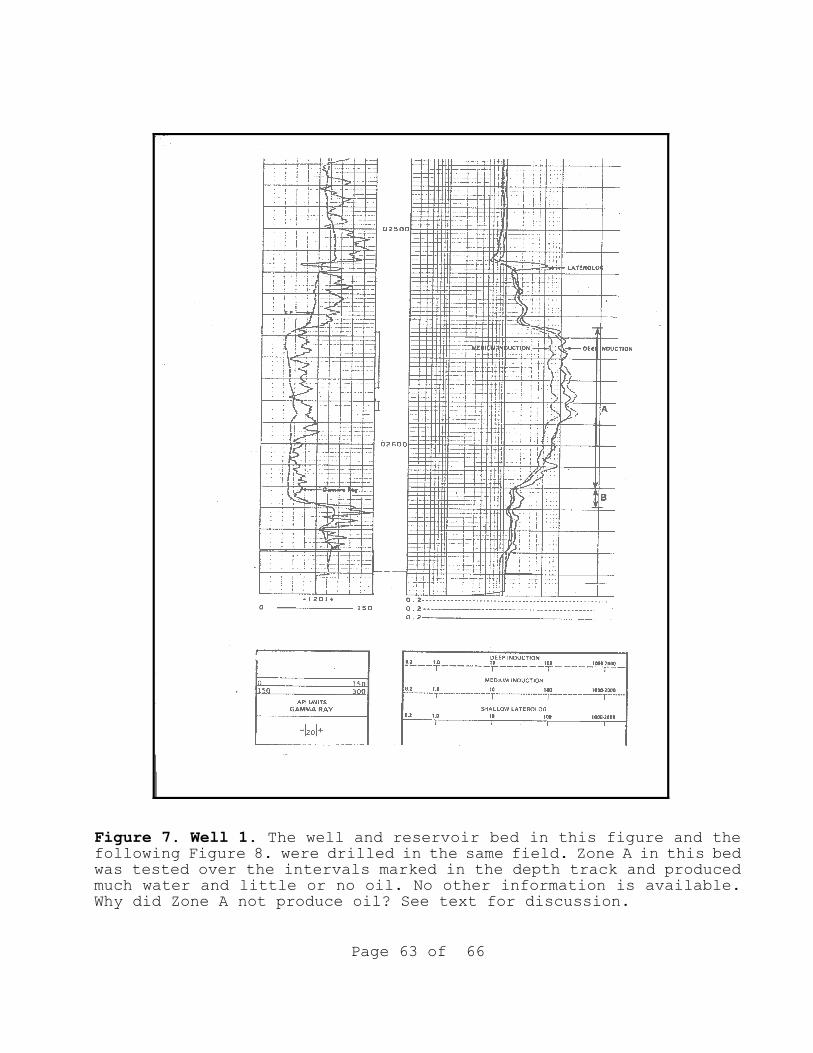
Page 63 of 66
Figure 7. Well 1. The well and reservoir bed in this figure and thefollowing Figure 8. were drilled in the same field. Zone A in this bedwas tested over the intervals marked in the depth track and producedmuch water and little or no oil. No other information is available.Why did Zone A not produce oil? See text for discussion.

Page 64 of 66
Figure 8. Well 2. The well and reservoir bed in this figure and thepreceding Figure 7 were drilled in the same field. No otherinformation is available for this well. Would Zone A produce oil? Seetext for discussion.

Page 65 of 66
Figure 9. Well 3. An example of a resistivity well log showing thepresence of both water and oil in a quality reservoir bed exhibitingconsiderably lower resistivity than in Wells 1 and 2. Zone A willproduce water-free oil. Why? Courtesy of Schlumberger.

Figure 10. Effectiveness of electrical interference by oil in oil-wet- and water-wet rocks. This figure is a chart of the behavior of Swt in response to the calculated values of exponent n (solid lines) from Well 1 (Figure 7), Well 2 (Figure 8), and Well 3 (Figure 9). This behavior is predicted by slope CG of triangle CDG of the model in Figure 1. See text for discussion and limitations of n.
Page 66 of 66