dsp algorithm overview 2008

DSP Algorithm and Low gComplexity Implementation

OverviewOverviewWonyong SungWonyong Sung

2 x 1.5 hrs

School of Electrical EngineeringSeoul National University

DSP Algorithms and Applications

FilteringLinear: FIR and recursive (IIR) ( )Nonlinear and time-varying: adaptive filterUsage: noise elimination, frequency compensation, sample rate conversion

TransformationFFT: frequency analysis, indirect convolutionDCT: real arithmetic, image/video processingDCT: real arithmetic, image/video processingUsage: spectrum analysis, OFDM(Orthogonal Frequency Division Multiplexing)

Communication blocksCommunication blocksNCO: digital oscillator, PLL: phase locked loopADC/DACADC/DACQPSK, QAM, OFDM, CDMA ECC: CRC, Hamming, BCH, RS, LDPC, convolutionalcoding

Wonyong SungMultimedia Systems Lab SNU

coding

Algorithm considerations for system designPerformance in terms of signal processing

For example, RLS is better than LMS in terms of signal robustness (adaptation speed)robustness (adaptation speed)…FIR is better in terms of phase linearity when compared with recursive filtering

For image processing, only FIR filtering is adequate.

Number of arithmetic ops.(multiplications)FIR filtering demands a lot of multiplicationsFIR filtering demands a lot of multiplications

But not always, for narrowband filtering, it needs a smaller one.

Algorithm complexity, parallel & regularitySeems more important in these days as there are abundant of arithmetic elements in a chip.Parallel structure is good for HW based design Parallel structure is good for HW based design.

If you start with a poor algorithm, there is not much way to recover the disadvantages!


You need to consider both performance and implementation characteristics.

Digital Filters

Types of Digital Filters: l b d hi h t hlow-pass, band-pass, high-pass, notch-filter, allpass, etc.

FIR and IIR Digital FiltersFIR and IIR Digital FiltersMultiplierless filtersFilters for sampling rate conversionFilters for sampling rate conversionStructures of Digital Filters

Direct, cascade, parallel forms, , pState-space realizationsOrthogonal digital filter

Quantization Errors, Stability, accuracy


Types of Digital Filters

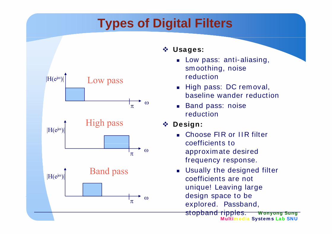
Usages:Low pass: anti-aliasing, smoothing, noise reductionHigh pass: DC removal,

|H(ejω)| Low passg p ,

baseline wander reductionBand pass: noise reduction

ωπ

Design: Choose FIR or IIR filter coefficients to

|H(ejω)|High pass

coefficients to approximate desired frequency response.Usually the designed filter

ωπ

Band pass Usually the designed filter coefficients are not unique! Leaving large design space to be ω

|H(ejω)|Band pass


design space to be explored. Passband, stopband ripples.

ωπ

Filter design and implementation

Filter design: determining the transfer function (H(z)) from the given frequency function (H(z)) from the given frequency domain specification. The location of poles and zeroes are determined. a d e oes a e dete edFilter implementation: determining the filter structure (direct form, 2nd order ( ,cascade form, …) , pole-zero pairing if needed, word-length and memory t t f d i th h d t structure for reducing the hardware cost,

machine cycles, or power consumption.


Digital filter specificationsDigital filter specifications

For example the magnitude response |G(ejω)| of a digital lowpass filter may be given as i di d b lindicated below


* Transition bandwidth is important for filter order determination.

Digital filter specificationsDigital filter specificationsIn practice, passband edge frequency and stopband edge frequency are specified in HzF di it l filt d i li d b d d

sF pF

For digital filter design, normalized bandedge frequencies need to be computed from specifications in Hz using

TFF

FF p

ppp π

πω 2

2==

Ω=

FF TT

TFF

FF s

sss ππω 22

==Ω

=FF TT


Digital filter specificationsDigital filter specificationsg pg p

In the passband we require that with a deviation

1)( ≅ωjeG δ±pωω ≤≤0

1)( ≅eG pδ±

ppj

p eG ωωδδ ω ≤+≤≤− ,1)(1In the stopband we require that

with a deviation ωj sδ

πωω ≤≤s

0)( ≅ωjeG

δω ≤≤≤jG )( πωωδω ≤≤≤ ssjeG ,)(



Filter specification parameters - passband edge frequencypω p g q y- stopband edge frequency- peak ripple value in the passband

p

sωpδ peak ripple value in the passband

- peak ripple value in the stopbandsδp



Practical specifications are often given in terms of loss function (in dB)terms of loss function (in dB)

)(log20)( 10ωω jeG−=G

Peak passband rippledB)1(l20 δ dB

Mi i t b d tt ti

)1(log20 10 pp δα −−=

Minimum stopband attenuationdB)(log20 10 ss δα −=


FIR, IIR digital filters

Let h[n: impulse response

Infinite impulse response (IIR) filter

QPp

x(n): input, y(n): outputFinite impulse response Both poles and zeroes.

1 0( ) ( ) ( ) ( ) ( )

QP

i ky n a i y n i b k x n k

= =

= − + −∑ ∑

Finite impulse response (FIR) filter: The length of impulse

(unitpulse)response may be infinite! R i f l ill

1

( ) ( ) ( )J

y n h j x n j−

= −∑Has only zeroes (no poles).

Recursive formula will impact on computation methods (feedback).Stability concerns:

0j=

Usually, implemented as a feed-forward type.

Stability concerns: The magnitude of y(n) may become infinity even all x(n) are finite!all x(n) are finite!coefficient values, quantization error


FIR filtersDirect form structure, which has a form of convolution, is usually used. Cascade or parallel forms are a little bit complex in terms of structure. The quantization effects of direct form FIR filters

till t l bl i t are still tolerable, in most cases. Symmetric coefficients FIR

Linear phase: critical for image p gprocessingHalve the # of multiplications

Filter designFilter designWindowingCAD – Parks McClellan method

The needed order is usually high. Good for interpolation, decimation filtering


g

Linear phase filter - symmetric FIRh(n) = h(-n)Evaluate the frequency response (assuming that N is odd) and h(n) is real-valued

1-N

h(n)

(N=7)

zh(n)=zh(n)=H(z)2

21-N

-=n

n-n

n=n

n- ∑∑2

1 n

)ee(h(n)+h(0)=)H(e

get weh(-n) = h(n) if

Ωn π2 j+Ωn π2 j-2

1-N

Ω π2 j ∑

]cos[h(n)2+h(0)=)H(e

)e-e(h(n) + h(0) =)H(e

21-N

Ωπ2j

1=n

∑

∑

]cos[h(n)2 + h(0) =)H(e Ωn π21=n

j ∑

The frequency response is real: phase shift is 0 or 180 degrees


q y p p g

Linear-phase type 1


Needed number of coefficients

For equiripple LP FIR filters:

se

F]

1log[

2=N

passstopstoppasse

F-F ]

DD10log[

3N

Independent of BW (Fpass)!p ( pass)Weak (logarithmic) dependence on the

Pass band ripple level and the Stop band iattenuation

Linear dependence on the transition band!O l N 29 ( d t 31)• Our example: Ne = 29 (compared to 31)

• Problem: Very narrow filters -> Decimating


Example

Develop an AM-SSB modulator using Simulink. There are a few methods for generating SSB signal. There are a few methods for generating SSB signal. Here you try to use a bandpass filter. The filter specification that I suggest is a bandpass filter having the following specification This filter is having the following specification. This filter is designed assuming that the message signal has the frequency range of 0.2KHz ~ 3.8KHz. Carrier freq = 12KHz Sampling freq = 48KHz= 12KHz, Sampling freq = 48KHz

f1: stopband edge: 11.8KHz f2: passband edge: 12 2KHz f2: passband edge: 12.2KHz f3: passband edge: 15.8KHz f4: stopband edge: 16 2KHz f4: stopband edge: 16.2KHz

Passband ripple: -0.5dB~+0.5dB, stopbandattenuation: 40dB


FIR filter design

Signal Processing Signal Processing Toolkit of MATLAB Define the frequency response template. response template. Case of LPF:

Pass band End Fpass

Pass band Ripple Dpass

Stop band Start F tStop band Start Fstop

Stop band Attenuation Dstop

Fstop-Fpass = Transition band


Design of EquirippleDesign of EquirippleDesign of Equiripple Design of Equiripple LinearLinear--Phase FIR FiltersPhase FIR Filters

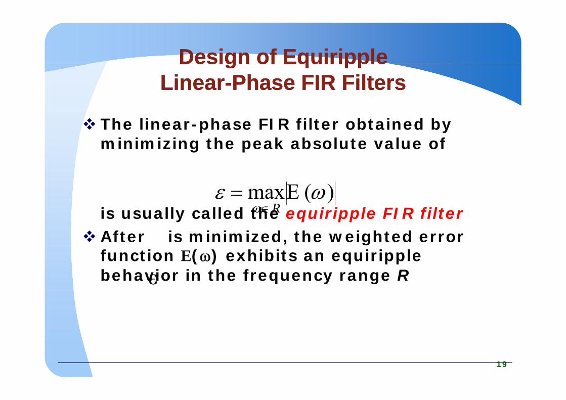
The linear-phase FIR filter obtained by minimizing the peak absolute value of

)(max ωε E=is usually called the equiripple FIR filterAfter is minimized, the weighted error

)(ω R∈

function E(ω) exhibits an equiripple behavior in the frequency range Rε

19

Design of Equiripple Design of Equiripple LinearLinear--Phase FIR FiltersPhase FIR Filters

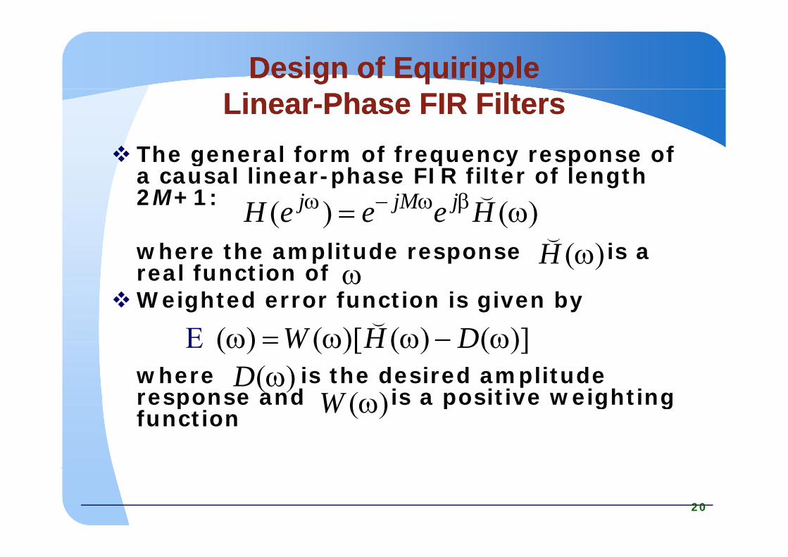
The general form of frequency response of The general form of frequency response of a causal linear-phase FIR filter of length 2M+1: )()( ω= βω−ω HeeeH jjMj (

where the amplitude response is a real function of

)()( ω= HeeeH)(ωH

(

ωreal function ofWeighted error function is given by

ω

)]()()[()( ω−ωω=ω DHW(

Ewhere is the desired amplitude response and is a positive weighting

)]()()[()( ωωω=ω DHW)(ωD

)(ωW

E

spo s d s pos g gfunction

)(ωW

20

Design of Equiripple Design of Equiripple LinearLinear--Phase FIR FiltersPhase FIR Filters

For filter designFor filter design,

⎨⎧=ω

passbandthein,1)(D

is required to satisfy the above ⎩⎨=ω

stopbandthein,0)(D

)(ωH(

is required to satisfy the above desired response with a ripple of in the passband and a ripple of in the

)(ωHpδ±

sδp ppstopband

s

21

Design of Design of EquirippleEquirippleLinearLinear--Phase FIR FiltersPhase FIR Filters

Thus, weighting function can be chosen either aseither as

⎨⎧ passbandthein,1

⎩⎨⎧

δδ=ω

stopbandthein,/p,

)(sp

W

or

⎨⎧ δδ passbandthein,/ ps

⎩⎨⎧ δδ

=ωstopbandthein,1passbandthein,/

)( psW

22

Example 1: Equiripple LP FIR (1)

LPF example:Pass band End Fpass = 0.1Pass band Ripple Dpass=0.05 (5%)Stop band Start F = Stop band Start Fstop= 0.13Stop band Attenuation D = 0 1 (1/10)Dstop = 0.1 (1/10)

Minimum of 31 coefficientsneeded to achieved required specificationsEven-symmetric impulse response


Example 1: Equiripple LP FIR (3)Pole-Zero plot in the z-planeFIR l t FIR -> pole at zero (causal)Location of zeros:

On the unit circle in the Stop bandFar from unit circle in Pass band -> ripples


FDAtool FIR design example


Edit, Convert Structure …


MATLAB example 1

N = 80; k = 0:(N-1); MATLAB filterb0 = 1;

b1 = -1;

MATLAB filtercommand

corresponds to the symbol Φb2 = 1;

B = [b0 b1 b2];

f = 1/8;

the symbol Φ

f = 1/8;

x = sin(2*pi*f*k+pi/6);

y = filter(B,1,x);

subplot(2,1,1)

systemFIR(0,0,4,5,10,'b')

subplot(2,1,2)

plot(k,x,'go', k,y,'bo',...

k x 'g-' k y 'b-')


k,x, g- , k,y, b- )

legend('input','output')

IIR or recursive filter

Utilize poles and zerosP l f h i b dPoles are for shaping pass bandsZeros are for stop bands

Th l h ld b i id f h i i l The poles should be inside of the unit circle in the z-domain for stability

Finite word length effects can affectFinite word-length effects can affectDirect forms are more susceptible.

U ll th d d d i ll h Usually, the order needed is smaller when compared to FIR filtersDirect forms are not good fixed point Direct forms are not good fixed-point implementations

2nd order cascade


2 order cascade, …

MATLAB example 3

N = 80; k = 0:(N-1);

a = 0.97;

B = [0 1];

A = [1 -a];

(k 0)

The impulse response does not vanish after

finite number ofx = (k==0);

y = filter(B,A,x);

subplot(3,1,1)

finite number of samples

p ( , , )draw1stIIR(0,0,4,5,10,'b')

subplot(3,1,2)stem(k,x,'r')( , , )ylabel('input')

subplot(3,1,3)stem(k,y,'b')


( ,y, )ylabel('output')

Basic 2nd Order IIR Structures

b(0)x(n) u(n) y(n) x(n) w(n) y(n)b(0)

b(1) −a(1) −a(1) b(1)z-1

z-1

z-1

z-1

z-1

-1

x(n-1) y(n-1)w(n-1)

Direct form I realization5 M l i l 4 Addi i ( )

Direct form II realization a.k.a BiQuad

b(2) −a(2) −a(2) b(2)z z z-1

x(n-2) y(n-2) w(n-2)

5 Multiply 4 Additions per y(n)4 registers storing x(n-1), x(n-2), y(n-1), y(n-2)

BiQuad5 multiply, 4 additions per y(n)2 registers storing w(n-1), w(n-2)

Different structures determines different execution order, different numerical properties, but retain the same algebraic relation between input

dWonyong Sung

Multimedia Systems Lab SNU

and output.

Cascaded and Parallel Structures

If the characteristic polynomial A(z) has real-

Cascaded realizationp y ( )valued coefficients, then it can be factorized as:

P ll l li ti

1 2

1 2 2 2

11 1 1 2 2

11 1 1 2P P

P P P Pz z r z r zγ ηγ

α α β− − − −− − − +

Parallel realization

1 2 1P Pk k zμ ν ρ −+∑ ∑1

2

1

1

( ) (1 )P

ii

P

A z zα −

=

⎛ ⎞= −⎜ ⎟⎝ ⎠

⎛ ⎞

∏ 1 1 2 21 1

( )1 1 2 cos

i k k

i ki k k k

zH zz r z r z

μ ν ρα β− − −

= =

+= +

− − +∑ ∑

2

1 2

1 2 2

1

(1 2 cos )

( ) ( )

k k kk

P P

r z r z

A z A z

β − −

=

⎛ ⎞⋅ − +⎜ ⎟⎝ ⎠

⎛ ⎞ ⎛ ⎞= ⋅⎜ ⎟ ⎜ ⎟

∏

∏ ∏1 1

1 2

( ) ( )i ki k

A z A z

P P P= =

= ⋅⎜ ⎟ ⎜ ⎟⎝ ⎠ ⎝ ⎠

= +

∏ ∏ +


2nd-order Sections

Generally implement high-order IIR filters as a sum or cascade of 2nd-order filters to reduce the sensitivity of the overall response to the precision of each coefficientthe overall response to the precision of each coefficientHigh-order polynomial is factored to find poles and zeros, and each 2nd-order filter (biquad) implements two zeros and two poles (real or complex conjugate)two zeros and two poles (real or complex conjugate)Poles and zeros are grouped in pairs—usually try to group in such a way that minimizes peak gain of each sectionIf cascaded, 2nd-order sections are usually ordered from lowest gain to highest gain to minimize overflow likelihoodScaling may be needed for overall response or for each section individually (computation vs. quality)

21

22

110

1)( −−

−−

++++

=zazazbzbbzH


211 ++ zaza

Pole-zero pairing

When pairing poles and zeros, it is better to combine nearby poles y pand zeroes for a same 2nd order structure. Purpose: to reduce the dynamic p yrange of internal signal

It is not good to magnify (attenuate) a signal and then (attenuate) a signal and then attenuate (magnify) it much in terms of quantization noise sensitivity. yCriteria: Maximal dynamic range: a ratio of (a) the maximum magnitude response computed ag tude espo se co putedover the whole frequency range to (b) the minimum magnitude response in the passband


p p

Implementation Issues

Coefficient quantizationDue to limited coefficients word-length. Due to limited coefficients word length. This affects the frequency response. Especially, the pass-band or stop-band ripple can be increasing (make a frequency distortion )increasing (make a frequency distortion.)

Roundoff error (least significant bits lost)Due to limited data word-lengthThis introduces random-like quantization noise. Make a noisier filter.

Limited data wordlengthx(n)

a(1)

w(n) y(n)b(0)

b(1)z-1Quantization of coefficients −a(1)

−a(2)

b(1)

b(2)z-1

w(n-1)

Q


w(n-2)

Engineering an IIR filter

Verify filter performance with quantized coefficientscoefficientsAssess roundoff error by modeling the truncation as a noise source in the filter structure. Determine the transfer function from each roundoff noise source transfer function from each roundoff noise source to the output.Calculate overflow situations by looking for peaks in frequency response from input to each accumulation point in the filter.


Cascade direct form II


Comparison of the complexity of different IIR filtersfilters

Wonyong SungMultimedia Systems Lab SNUFrom: Miodrag Bolic

Further reading

M. D. Lutovac, D. V. Tošić, B. L. Evans

Filter Design for Signal ProcessingFilter Design for Signal Processing Using MATLAB and Mathematica

Prentice HallPrentice HallUpper Saddle River, New Jersey ISBN 0-201-36130-2, (c) 2001, ( )

http://kondor etf bg ac yu/~lutovac/Wonyong Sung


http://kondor.etf.bg.ac.yu/ lutovac/

Multiplierless filters

IntegratorH(z) = 1/1-z-1H(z) 1/1 z

Integrator has a pole at z=1, so it is a kind of lowpass filter with no multiplier Should be with no multiplier. Should be careful for overflow due to DC accumulation. x[n] y[n]

Moving average (MA) filterH(z) = (1-z-N)/(1-z-1)

MA filter has many zeroes MA filter has many zeroes around the unit circle except for z=1. It is a lowpass filter. It can be modified to a It can be modified to a bandpass or highpass filter. = 1+z-1+z-2+… +z-(N-1)


Good for FPGA’s with DSP blocks

Two moving averager implementations

Feed-forward type:Higher number of z-1 z-1 z-1x[n]Higher number of arithmetic operationsBetter stability

z z z

y[n]

x[n]

ette stab tyFeed-back type:

Lower number of x[n]

[ ]

z-N

arithmetic operationsShould be careful against overflows

y[n]

z-1

against overflows

Both structures have Both structures have the same frequency response with infinite

i i i h iWonyong Sung


precision arithmetic

Key points

Different types and structures of digital filters may achieve the same or similar goals, but with gdifferent implementation costs, numerical propertiesDesign space that can be exploredg p p

Filter types: FIR, IIR, adaptive filtersSpecifications/performance goalsFilter structuresFilter structures

Direct, parallel, cascade …Numerical properties (floating point/fixed point, etc.)


Interpolation (Sample rate increase)

Insert N-1 zeroes between the samples, then conduct lowpass filtering (pi/N) then conduct lowpass filtering (pi/N). Among N tap inputs, only one is non-zero (no need to compute N-1 mult )(no need to compute N 1 mult.)


Decimation (Sample rate reduction)Conduct lowpass filtering (pi/N).Among N output samples, select only one. So, we do not need to compute N-1 output samples. do not need to compute N 1 output samples.

(This is not possible for recursive filters because of feedback!)


FIR filter implementation for decimation, interpolationp

For interpolation: (N-1) among N input values at the tap are zero! No need to values at the tap are zero! No need to conduct multiplicationsFor decimation: We only need to compute 1 For decimation: We only need to compute 1 output sample at every N output. It is interpreted as polyphase filter with It is interpreted as polyphase filter with the tap length of about M/N.


Here's an example of a 12-tap FIR filter that implements i l i b f f f Th ffi i h0 h11 dinterpolation by a factor of four. The coefficients are h0-h11, and three data samples, x0-x2 (with the newest, x2, on the left) have made their way into the filter's delay line:

h0 h1 h2 h3 h4 h5 h6 h7 h8 h9 h10 h11 Result

x2 0 0 0 x1 0 0 0 x0 0 0 0 x2·h0+x1·h4+x0·h8

0 x2 0 0 0 x1 0 0 0 x0 0 0 x2·h1+x1·h5+x0·h9

0 0 x2 0 0 0 x1 0 0 0 x0 0 x2·h2+x1·h6+x0·h10

0 0 0 x2 0 0 0 x1 0 0 0 x0 x2·h3+x1·h7+x0·h110 0 0 x2 0 0 0 x1 0 0 0 x0 x2·h3+x1·h7+x0·h11


FIR filtering for narrowband signal

Narrow band filtering (large order needed): It is advantageous to conduct decimation It is advantageous to conduct decimation followed by post-filtering (operates at low sampling rate) -> the total number of sa p g ate) > t e tota u be omult’s is reduced.Application to IF filtering for digital radiopp g g


Example with SSB generation

What if the carrier frequency for AM in HW#1 is 2 048KHz Assume that the HW#1 is 2,048KHz. Assume that the sampling frequency for the carrier is 4*2,048KHz. ,0 8Design the bandpass filter for removing the lower sideband.Assume that the message signal has the sampling frequency of 8KHz. Design the interpolation filter for interpolating the message signal. C id h t d d l t h Consider a heterodyne modulator, where the 1st stage modulation frequency is 12KHz The generated SSB is then 12KHz. The generated SSB is, then, modulated to 2,048KHz.


Discussion

FIR filter can be implemented using direct

There are numerous possible realization t t f th

p gform or fast convolution methods like FFT.IIR filters are often

structures of the same digital filters. Digital filter coefficients are not always exact It is

factored into products (cascade realization) or sum (parallel realization)

are not always exact. It is possible to realize a digital filter with the same desired properties

of 1st order or 2nd order sections due to numerical concerns.

p pbut different filter structures and coefficients to exploit favorable implementation favorable implementation alternatives. A state space model is a good example.p


Quantization error, stability, overflowAn IIR filter is BIBO stable if all the poles of its transfer function H(z)

OverflowDynamic range of its transfer function H(z)

lie within the unit circle in z-plane.A stable IIR digital filter

y gintermediate results must be bounded.Otherwise, overflow h k t b d d may become unstable

when its coefficients are subject to severe quantization due to finite

check must be used and that is very costly. Saturation arithmetic may reduce the error quantization due to finite

length of registers. Hence an IIR filter that is stable when designed

may reduce the error caused by overflow.

is stable when designed with a 32 bit machine may become unstable when implemented with

8 bit i t ll !an 8-bit micro-controller!


Adaptive filter and adaptive signal processingadaptive signal processing

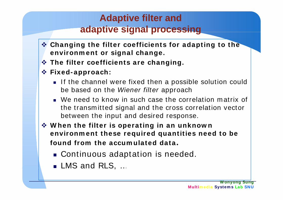
Changing the filter coefficients for adapting to the environment or signal change. environment or signal change. The filter coefficients are changing. Fixed-approach:

If the channel were fixed then a possible solution could be based on the Wiener filter approachWe need to know in such case the correlation matrix of We need to know in such case the correlation matrix of the transmitted signal and the cross correlation vector between the input and desired response.

h h fil i i i kWhen the filter is operating in an unknown environment these required quantities need to be found from the accumulated data.

Continuous adaptation is needed. LMS and RLS, …


LMS and RLS, …

Adaptive signal processing

A possible framework is:A possible framework is:

][ndDesired signal

Input signal ][nd][ˆ nd][ nx Adaptive

Input signal

][new:Filter

Minimize the error signal

Algorithm


Applications of adaptive filters

Applications are manyDigital CommunicationsDigital CommunicationsChannel EqualisationAdaptive noise cancellationcancellationAdaptive echo cancellationS id ifi iSystem identificationSmart antenna systemsBlind system equalisationy qAnd many, many others


Echo cancellers in local loops

Tx1 Tx2

Echo canceller Echo cancellerHybrid Hybrid

Adaptive Algorithm Adaptive AlgorithmLocal Loop

-

+

-

+Rx1 Rx2


+ +

Adaptive noise canceller

FIR filter

REFERENCE SIGNAL

Noise

-

FIR filter

+Adaptive Algorithm

Signal +Noise

PRIMARY SIGNAL



Adaptive Arrays

Linear CombinerLinear Combiner

Interference


Adaptive signal processingBasic principles:1) Form an objective function (performance 1) Form an objective function (performance criterion)2) Find gradient of objective function with respect to FIR filter weightsto FIR filter weights3) There are several different approaches that can be used at this point3) Form a differential/difference equation from the 3) Form a differential/difference equation from the gradient.



Let the desired signal beThe input signal

][nd][nxp g

The outputNow form the vectors

][nx][ny

So that[ ]Tmnxnxnxn ]1[.]1[][][ +−−=x

[ ]Tmhhh ]1[.]1[]0[ +=h

hx Tnny ][][ =Objective function

[ ] ][][)( 2nyndEJ =w

hx nny ][][ =

[ ] ][][)( nyndEJ −=w

Rhhphhpw TTTdJ +−−= 2)( σ


][][ TnnE xxR =][][ ndnE xp =


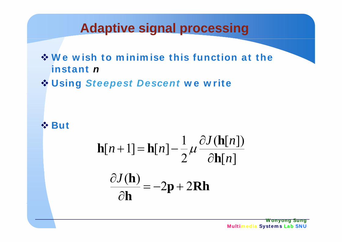
We wish to minimise this function at the i t t instant nUsing Steepest Descent we write

But

])[(1][]1[ nJnn hhh ∂=+ μ][2

][]1[n

nnh

hh∂

−=+ μ

h)(∂J Rhphh 22)( +−=

∂∂J



So that the “weights update equation”

Since the objective function is quadratic this

])[(][]1[ nnn Rhphh −+=+ μj

expression will converge in m stepsThe equation is not practicalIf we knew and a priori we could find the pRIf we knew and a priori we could find the required solution (Wiener) as

pR

pRh 1−= pRh =opt


Adaptive signal processingHowever these matrices are not knownApproximate expressions are obtained by ignoring Approximate expressions are obtained by ignoring the expectations in the earlier complete forms

This is very crude. However, because the update equation accumulates such quantities, progressive we expect the crude form to improvewe expect the crude form to improve

Tnnn ][][][ˆ xxR = ][][][ˆ ndnn xp =nnn ][][][ xxR ][][][p


The LMS algorithm

Thus we have

])[][][]([][]1[ nnndnnn T hxxhh −+=+ μWhere the error is

])[][][]([][]1[ nnndnnn hxxhh −+=+ μ

])[][(])[][][(][ nyndnnndne T −=−= hxAnd hence can write

hi i i ll d h h i di

])[][(])[][][(][ y

][][][]1[ nennn xhh μ+=+This is sometimes called the stochastic gradientdescent


Convergence

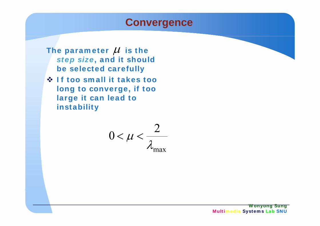
The parameter is the step size, and it should

μstep size, and it should be selected carefullyIf too small it takes too long to converge if too long to converge, if too large it can lead to instability

20 μ <<max

0λ

μ <<


Convergence

We require that

Or 11 max <− μλ

In practice we take a much smaller value than thisthan this

20λ

μ <<maxλ


Transform based LMS

][nd][ˆ nd][ nx

][w:Filter

Adaptive

][ne

AlgorithmTransform gTransform

Inverse Transform


Least squares adaptive

with

∑n Tii ][][][R

We have the Least Squares solution

∑==i

Tiin1

][][][ xxR

However, this is computationally very intensive to implement. ∑=

nndnn ][][][ xp

Alternative forms make use of recursive estimates of the matrices involved.

∑=i 1

][][][p

][][][ 1 ][][][ 1 nnn pRh −=


Recursive Least Squares

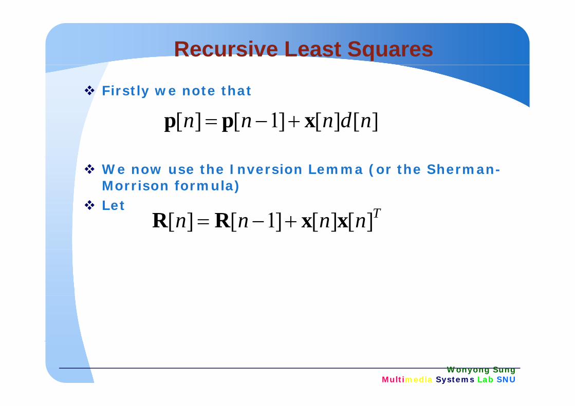
Firstly we note that

][][]1[][ ndnnn xpp +−=

We now use the Inversion Lemma (or the Sherman-Morrison formula)Let Let Tnnnn ][][]1[][ xxRR +−=


Recursive Least Squares (RLS)

Let1][][ −nn RP

Then ][]1[ 1 nn xR −−

][][ = nn RP

h i i k h l i

][]1[][1][]1[][ 1 nnn

nnn T xRxxRk −−+

=

The quantity is known as the Kalman gain

]1[][][]1[][ −−−= nnnnn T PxkRP

][nk


Recursive Least Squares

Now use in the computation of the filter weights

][][][ nnn xPk =

From the earlier expression for updates we have

])[][]1[]([][][][ ndnnnnnn xpPpPh +−==][nP

And hence

][nP]1[]1[][][]1[]1[]1[][ −−−−−=− nnnnnnnn T pPxkpPpP

And hence

])1[][][]([]1[][ −−+−= nnndnnn T hxkhh


Transforms

School of Electrical EngineeringSeoul National University

Linear transformations

Signals represented in the frequency domain

Linearity: Let T[x] be the linear transform of q y

have different properties that can be exploited to facilitate ffi i di i l i l

signal sequence x. Then for arbitrary constant a, b

efficient digital signal processing A linear transform is a Types of linear

1 2 1 2[ ] [ ] [ ]T ax bx aT x bT x+ = +

mapping that converts time domain (or spatial domain) digital signal i f d i

Types of linear transforms

DFT: discrete Fourier transforminto frequency domain

coefficients.A linear transform

transformDCT: discrete cosine transformDWT di l operates on the entire

sequence of digital signals.

DWT: discrete wavelet transformKLT: Optimal linear


transform

Matrix Formulations

1D linear transformRepresent a finite 1D

2D linear transformOften consider 2D separableRepresent a finite 1D

sequence by a column vector:

The 1D linear transform can

plinear transform. That is a 1D linear transform is first applied to each row of the 2D signal and then a second [ ]TNxxxX ][]2[]1[ L=The 1D linear transform can

be represented as a matrix-vector product:

2D signal, and then a second 1D transform is applied to each column of the transformed signal. It

[ ]][][][

where T is a N × N matrix whose elements may be

l l d

t a s o ed s g a tconsists of two consecutive matrix-matrix product:

XY ⋅= T

complex-valued. U and V are the transformation matrices

VXUY ⋅⋅=


Discrete Fourier Transform

The 1D DFT is defined as: 1

( ) ( )N

mkY k X W−

∑for 0 ≤ m ≤ N−1, where the data X(m); 0 ≤ m ≤ N−1

Each complex-valued arithmetic:

0( ) ( ) mk

Nm

Y k X m W=

= ∑

may be real-valued or complex-valued, and Requires N2 complex-valued MAC ti 4N2 l

Requires 4 real-valued multiplications and two

( )( ) ( ) ( )a jb c jd ac bd j bc ad+ + = − + +

MAC operations, or 4N2 real-valued MAC operations.Fast Fourier Transform (FFT) can reduce the DFT

multiplications and two additions.Half if one operand is a real numbercan reduce the DFT

computation to O(N log N)number.

Special arithmetic algorithms s ch as CORDIC can be sed such as CORDIC can be used to implement complex-valued multiplication effectively.

( )NjWN /2exp π−=


⎪⎧

−=⋅=∑− −

110][][:DFT1 2

NkenxkXN n

Njk

Lπ

⎪

⎪⎪⎨

−=⋅=

∑

∑−

=

110][1][IDFT

1,,1,0,][][: DFT

1 20

NkX

NkenxkX

N nN

jk

nL

π

⎪⎪⎩

−=⋅⋅= ∑=

1,,1,0,][1][: IDFT

2

0NnekX

Nnx

j

k

N L

π

⎧

=−

−,thenNotation Use-

1

eWN

Nj

N

⎪

⎪⎪⎨

⎧−=⋅=∑

=

1

1,,1,0,][][: DFT

10

NkWnxkX

Nn

knN L

⎪⎪⎩

−=⋅⋅= ∑−

=

− 1,,1,0,][1][: IDFT1

0NnWkX

Nnx

N

k

knN L


BGL/SNU

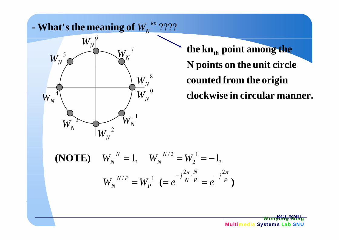
????knNW of meaning the s What'-

6W

circleunittheonpointsN the amongpoint kn the th5

NW

6NW

7NW

i lil k i origin the from counted

circleunit theonpoints N

0W4

8NW

manner.circular inclockwise0NW

1W3

4NW

NW2

NW3

NW

(NOTE)jNj

NN

NN WWW

ππ 22

12

2/ ,1,1 −===

)( Pj

PNj

PPN

N eeWW 1/ −⋅−===


BGL/SNU

2. Decimation-in-Time Factorization2. Decimation in Time Factorization

1

)2(1,,1,0,][][N

knN NNkWnxkX

−

∑ =−=⋅= υL

.0

)2(1,,1,0,][][

DFTptNn

N NNkWnxkX

−=

∑∑

∑

+

12/)12(

12/2

,,

Nkr

Nrk

oddnevenn

−+

−

∑∑

∑∑ +=

12/12/0

)12(

0

2 ]12[]2[

Nkk

Nk

r

krN

r

rkN WrxWrx

−−

=

+

=∑∑ ++=

)(,.2/0

2/

)(,.2/0

2/ ]12[]2[

kHDFTptNr

rkN

kN

kGDFTptNr

rkN WrxWWrx

−=

−=

∑∑ +⋅+=


BGL/SNU

8)( =Neg]0[ ]0[X]0[x]1[x

]0[X]1[X

pt.-N

]7[x ]7[XDFT

]0[ ]0[XN]0[G 0W]0[x

]2[x]4[x

]0[X]1[X]2[XDFT

pt.-2N

][

]1[G]2[G]3[G

NW1

NW

3W

2NW

DFT ]3[X]6[x ]3[G NW

]1[x]3[x]5[

]4[X]5[X]6[X

pt.-2N

]0[H

]1[H]2[H

4NW

5NW

6W


]5[x ]6[XDFT ]7[X]7[x

]2[H]3[H

NW7

NWBGL/SNU

graph flow Final

]0[x]2[x

]0[X]1[X

0NW

1NW

2W

0NW

4W

0NW

2W

000100

000001][

]4[x]6[x

]2[X]3[X

3NWNW

4W

0NW

4NW

NW 2NW

4NW

6NW

010110

010011

]1[x]3[x

]4[X]5[X

NW5

NW6

NW

0NW

4NW

NW N

0NW

2W

001101

100101

]5[x]7[x

]6[X]7[X

NW7

NW0

NW4

NW

NNW

4NW

6NW

011111

110111

)( reversedbit − )(natural


BGL/SNU

Fast Fourier Transform

Decimation in time formulation

If L(N) = # of ops for Npt FFT, and N = 2m, then

Function Y = fft(N,x)If N==1, Y = x;Else

L(N) = N + 2*L(N/2)= N + 2*[N/2 + 2*L(N/22)]= 2N + 22*L(N/22)= = mN + 2m L(N/2m)xeven=[x(0)x(2)… x(N-2)];

xodd=[x(1) x(3) … x(N-1)];Yeven=fft(N/2,xeven);Yodd=fft(N/2 xodd);

= … = mN + 2m L(N/2m)= (m+1)N ~ O(N log2N)

Basic computation unit: twilde factor (each operation)Yodd=fft(N/2,xodd);

For k=0:N-1,Y(k)=Yeven(k mod N/2) + Wk*Yodd(k mode N/2);

twilde factor (each operation)4 multiply, 4 addition

endend

⎡ ⎤ ⎡ ⎤ ⎡ ⎤⎡ ⎤cos sinsin cos

2 /

r r r

i i i

p q sp q s

k N

θ θθ θ

θ π

−⎡ ⎤ ⎡ ⎤ ⎡ ⎤⎡ ⎤= +⎢ ⎥ ⎢ ⎥ ⎢ ⎥⎢ ⎥⎣ ⎦⎣ ⎦ ⎣ ⎦ ⎣ ⎦

=


2 /k Nθ π=

Nlogstages#:processingcascaded-Remarks

==•

υN/2/stage# : sbutterflie -

Nlogstages#:processingcascaded 2

===υ

1

8W

5W1

8W

1

1−

y1/butterfly2/butterfl:tionsmultiplica(complex) nscomputatio # -

⎧ →

8W 8

(complex)nscomputatioof#total/butterflyy2/butterfl : additons

y1/butterfly2/butterfl:tionsmultiplica

⎩⎨⎧

→→

2

N/21 : tionsmultiplica

(complex)nscomputatioof # total

⎪⎨⎧ =⋅⋅ NN

2log2

υ

scompuationphase-in-N/22 : additons

⎪⎩⎨

=⋅⋅ NN 2log2

υ


reversed.-bit : ordering datainput - scompuationphase-in -

BGL/SNU

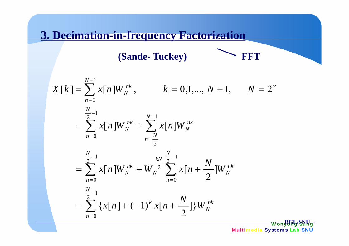
3. Decimation-in-frequency Factorization

(Sande- Tuckey) FFT

q y

Nnk

N NNkWnxkX 2 ,1,...,1,0 ,][][1

=−== ∑−

ν

Nnk

N

nk

n

WW ][][11

2

0

∑∑

∑

−−

=

NN

Nn

nkN

n

nkN WnxWnx ][][

20

+= ∑∑==

N

nkN

kN

N

N

nkN WNnxWWnx ]

2[][

12

0

2

12

0++= ∑∑

−−

nkk

Nnn

WNnxnx ][)1(][

21

2

00

+−+= ∑−

==


Nn

Wnxnx ]2

[)1(][ 0

++= ∑=

BGL/SNU

Final flow graphFinal flow graph

X[0][0] X[0]

X[4]

x[0]

x[1]0W1

X[2]

X[6]

x[2]

x[3]

0NW 1−

0NW 1−

X[6]

X[1]

x[3]

x[4]0NW 1−

2NW 1− 0

NW 1−

X[5]

X[3]

x[5]

x[6] 2

1N

N

W 1− 0NW 1−

[ ]

X[7]

[ ]

x[7] 3N

2N

W 1

W 1

−

−

2N

0N

W 1

W 1

−

−

0NW 1−


N

BGL/SNU

-Remarkslog: 2 N=ν

:

log: 2

N

N ν- # Stages

# b tt fli

)(log:

2:

complexNN

- # butterflies

- # computations )(log2

: 2 complexN# computations

- inplace computations- output data ordering : bit-reversed

-QuestionThe flow graph for D-I-F is obtained by reversing.

The direction of the flow graph for D-I-T. Why?


-Omit Sections 9.5-9.7BGL/SNU

4. Applications of FFT

(1) Spectrum Analysis1N −

-

is the spectrum of x[n] n=0 1 N-1

1,...,1,0, ][k][ 0

Nk WnxX n

nkN∑

=

−==

is the spectrum of x[n] , n 0,1,…,N 1

- Inverse transform can be done through the same mechanism

i) Take the complex conjugate of X[k]ii) Pass it through the FFT processii) Pass it through the FFT process,

But with one shift right(/2) operation at each stageiii) Finally take the complex conjugate of the resultiii) Finally, take the complex conjugate of the result

]][1[][1x[n]11

WkXWkX N

nkN

Nnk

N ∑∑−

∗∗−

− == ν


]][2

[][[ ]00

N k

Nk

N ∑∑==

ν

BGL/SNU

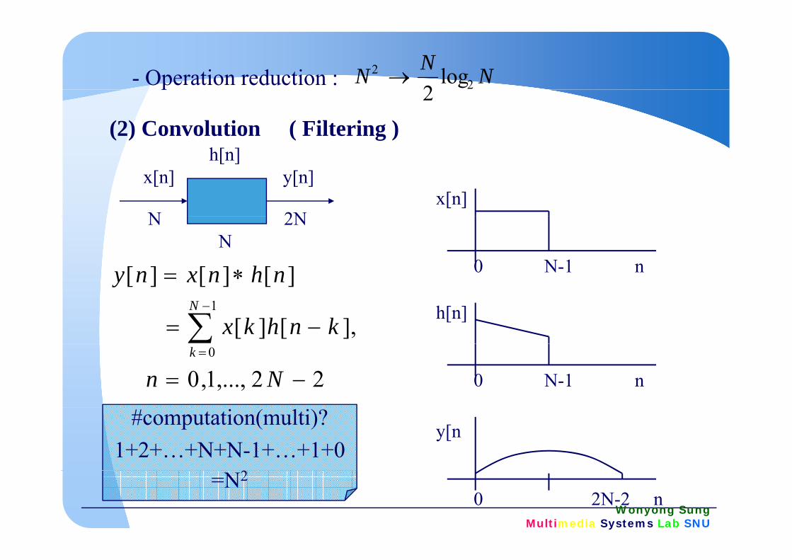
- Operation reduction : NNN 22 log

2 →

(2) Convolution ( Filtering )

p2

h[n]h[n]x[n] y[n]

N 2Nx[n]

N 2NN

0 N-1 n ][][][ ∗= nhnxnyh[n] ],[][

][][][1

−= ∑−

knhkx

nhnxnyN

0 N-1 n 22,...,1,0 0

−==

Nnk

y[n#computation(multi)?

1+2+…+N+N-1+…+1+02


0 2N-2 n =N2

-Utilize FFT of 2N-point~x[n]

h[ ]

0 N-1 2N n

~ [n]]][~][~[

][][~][12

2

Rknhkx

nRnynyN

N∗=

∑−

h[n]

12,...,1,0

[n],]][][[0

2

Nn

Rknhkxk

N

−=

⋅−= ∑=

0 N-1 2N n

R2N[n] ][][][

, ,,

kHkXkY ⋅=1

0 2N-1 n

],[][][ kHkXkY ⋅=2N-pt DFTs

y[n]~


0 2N-2 2N n BGL/SNU

2N pt X[k]2N-ptFFT

2N-pt

x[n]X[k]

Y[k]y[n]

2N-ptFFT

IFFTh[n]

H[k]

y[n]

H[k]

NN 2log22

NN 2log2

2 22NN2log2

2 2 2

# operation (multi)# operation (multi)

NNNNNN 5log322log2

23 22 +=+⋅

- operation reduction : NNN 5log3N 22 +=


000,35 000,000,1 :21024N 10 →==BGL/SNU

(3) Correlation /Power Spectrum][][][

1

nhnxnzN −

∗ −∗=

(3) Correlation /Power Spectrum

][][

1

1

0knhkx

N

N

k−

=

∗ +−= ∑

12210

[n] ]][~][~[ 1

02

Nn

RknhkxN

kN

=

∗ ⋅+−= ∑

][][][

12,...,2,1,0

kHkXkZ

Nn

∗

−=

2N i DFT

],[][][ kHkXkZ ∗⋅= 2N-point DFTs

# Operation : NNN 5log3N2 +→# Operation : NNN 5log3 N 2 +→

- Power spectrum P[k] = X[k] X*[k]


BGL/SNU

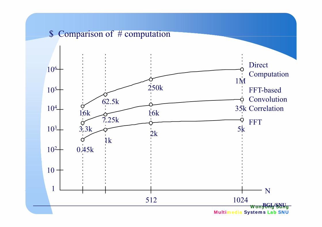
$ Comparison of # computation$ Comparison of # computation

106

105 250k1M

DirectComputation

FFT b d

104

105

35k16k16k62.5k

250k FFT-basedConvolutionCorrelation

103

1k2k 5k

16k7.25k

3.3k

16kFFT

102 0.45k1k

1

10

N


512 10241 N

BGL/SNU

Discrete Cosine/Sine Transform

DCT: Fast DCT see note: fastdct.doc

DST

Both DCT and DST can be expressed as Matrix-

1 (2 1)( 1)( ) ( ) iN m uG π− + +∑expressed as Matrix-

vector products.1 (2 1)( ) ( ) ( ) cos

2

N m uF u u x mNπα

− += ∑

0

( )( )( ) ( )sin1m

G u x mN=

=+∑

2D DCT

0 21 1 1

( ) ;1/ 2 0

m Nu N

uu

α

=

≤ ≤ −⎧⎪= ⎨=⎪⎩1/ 2 0u⎪⎩

1 1

0 0

2 (2 1) (2 1)( , ) ( ) ( ) ( ) ( ) cos cos2 2

N N

m n

m u n nF u v u v x m x nN N N

π πα α− −

= =

+ +⎧ ⎫ ⎧ ⎫= ⎨ ⎬ ⎨ ⎬⎩ ⎭ ⎩ ⎭

∑∑


5 Fast Computation of DCT

)(1 kN

5. Fast Computation of DCT

1,...,1,0, 2

)12(cos][][2k][ 1

0−=

+= ∑

−

=

Nk N

knnxkeN

X N

k

π

0k,2

1 ][ == ke

otherwise, 1

∑−

−=+

=1

1,...,1,0, 2

)12(cos][][n][ N

Nn N

knkXkex π∑=0 2k N


BGL/SNU

- Example: Lee’s Algorithm (1984, IEEE Trans , ASSP, Dec)

x[0]

x[1]

X[0]

X[4] x[1]

x[2]

X[4]

X[2] 1− 1b

1− 1 a

x[3]

x[4]

X[6]

X[1] 1

1

− 3

1

b 1− 1a

x[5]

[6]

X[5]

X[3]

1

1

−

−

3

1

cc

1− 1ax[6]

x[7]

X[3]

X[7]

1

1

−

−

5

7

cc

1

1− 1

b

b1−a 1 5c 1− 3b 1− 1a

3,1 ,1 1 1 === iiba i ππ7,5,3,1,1 iici == π


8cos2

4cos2

1 ii ππ

16

cos2

iπ

BGL/SNU

Discrete Wavelet Transform

H0(z), H1(z): low pass and high pass FIR digital filters. Maintain same number of input samples and output samples↓2: down-sampling by a factor 2.

↓ ↓ ↓H0(z) ↓2

H1(z) ↓2

H0(z) ↓2

H1(z) ↓2

H0(z) ↓2

H1(z) ↓2

x(n) y1(n)

y2(n)

y3(n)

y4(n)


-1

y[n]x[n]

z-1a

-1


dsp algorithm overview 2008

Documents