Drivers of Escape and Descent: Changing Household Fortunes in Rural Bangladesh

Binayak Sen Bangladesh Institute of Development Studies E-17 Agargaon Sher-e-Bangla Nagar Dhaka 1207 Bangladesh Phone: 880-2-911 7829 Fax: 880-2-811-3023 Email: bsen@bdonline.com and bsen@sdnbd.org

2

Drivers of Escape and Descent: Changing Household Fortunes in Rural Bangladesh

BINAYAK SEN Bangladesh Institute of Development Studies

Summary - This paper analyses a panel dataset on 379 rural households in Bangladesh

interviewed in 1987/88 and 2000. Using a ‘livelihoods’ framework it contrasts the fortunes of

ascending households (which escape poverty) and descending households (which fall into

poverty). These two dynamics are not mirror images of each other. Escapees overcome

structural obstacles by pursuing multiple strategies (crop intensification, agricultural

diversification, off-farm activity, irrigation) that permitted them to relatively rapidly

accumulate a mix of assets. Descents into poverty were associated with lifecycle changes

and crises such as flooding and ill-health. The findings confirm that Bangladesh made great

progress in reducing poverty in the 1980s and 1990s.

Keywords: Asia, Bangladesh, chronic poverty, vulnerability, rural livelihoods

• The author wishes to express sincere appreciation to Manik Lal Bose for his support in processing the data.

Very useful comments received from two anonymous referees are gratefully acknowledged. Successive

discussions with David Hulme and Mahabub Hossain have immensely helped to clarify the issues involved

in understanding poverty transitions. Financial support from the Department for International

Development’s (DFID) Social Science Research Grant (R7847) and DFID (Bangladesh) are gratefully

acknowledged.

I. INTRODUCTION

3

Changes in the incidence of poverty at the aggregate level can at best be considered as the

summary measure of net changes in the well-being of a given population. What they do not

take into account is that the group of poor people is itself constantly changing. Individuals

and households escape from poverty and descend into poverty. Two considerations are

relevant here. First, what explains the movement (mobility) or lack of movement

(immobility), in and out of poverty for different households with fluctuating fortunes?

Second, the analysis of changes in the aggregate level of poverty based on conventional

household income expenditure survey (HIES) data typically highlight the importance of

certain groups of policies and institutional actions. How well do they explain the slippage

into and escape from poverty? As is known, HIES data cannot be used to track the poverty

dynamics of specific households over time and space. In this paper we address these two

questions with household level panel survey data. The data for the analysis is provided from a

survey of 21 villages in Bangladesh consisting of a representative panel of 379 households

selected through a multi-stage stratified random sampling method. 1 The survey was carried

out in 1987/88 with a re-survey of the same households in 2000. The analysis of escape and

descent of the panel households adopts the ‘rural livelihoods’ framework (Ellis, 2000). Policy

implications derived from this analysis can help formulate more effective policies for

attacking poverty. In this paper there is a particular focus on policies to reduce chronic

poverty.

The paper has seven sections. After this brief introduction the second section summarises the

stylized findings from conventional poverty trends profile-determinants analysis in

Bangladesh2 to set the stage for the subsequent discussion on dynamic aspects of poverty.

The third section examines the poverty trends based on the panel survey and identifies several

‘dynamic poor’ groups on the basis of their diverse movements in and out of poverty. Section

4

four highlights the key characteristics of these groups with a special focus on the asset base

and income of the chronic poor.3 The fifth section presents the main findings of the paper

relating to the ‘drivers of escape’ by analysing the experience of the households that have

crossed the poverty line during the inter-survey period. The sixth section focuses on the

‘drivers of descent’ by tracking the changes experienced by the households who were non-

poor in the first period, but slipped into poverty by 2000. The final section presents the major

conclusions.

2. POVERTY IN BANGLADESH: OVERVIEW OF STYLIZED ASPECTS

(a) Trends in poverty

Trends in poverty are discussed in both income and non-income dimensions. Five aspects are

noteworthy. First, Bangladesh has made considerable progress in income-poverty reduction

since Independence.4 The proportion of population living below the poverty line was as high

as 74 percent in 1973/74. The income-poverty trends since the early nineties show the

following pattern. Between 1991/92 and 2000, the incidence of national poverty declined

from 50 to 40 percent, indicating a reduction rate of 1 percent per year. The declining trend is

robust to the choice of poverty measures (Table 1).

[Table 1 here]

Second, the results broadly indicate that progress was greater during the 1990s than the

1980s. This faster pace of poverty reduction is attributable to the accelerated growth in

consumption expenditure (income).5 Third, the comparative progress was uneven between

5

rural and urban areas. The pace of rural poverty reduction was slow in the 1980s, but became

considerably faster in the 1990s. The pace of urban poverty reduction was only slightly

higher in the 1990s compared to the 1980s.

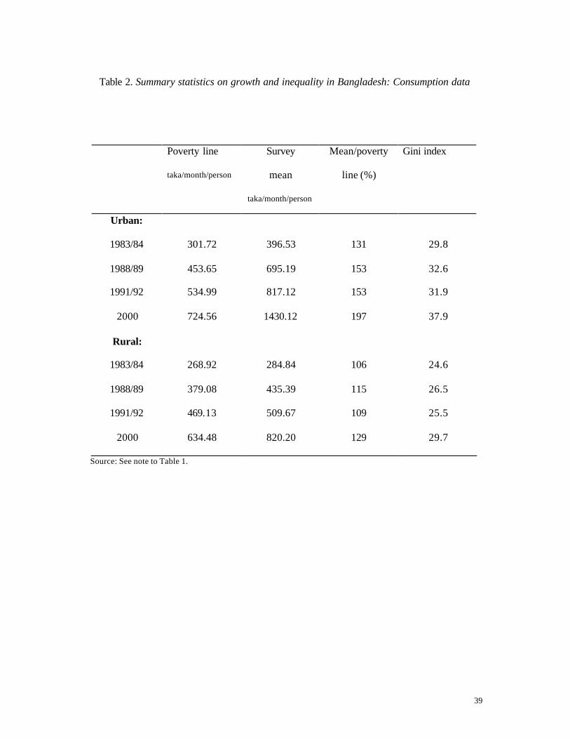
Fourth, poverty trends are influenced by changes in inequality. The level of inequality, as

measured by consumption expenditure distribution, showed very little change during the

1980s but during the 1990s the Gini coefficient rose considerably, with urban inequality

rising much more than rural inequality (Table 2). Thus, during the period 1991/92 to 2000,

the level of consumption expenditure inequality increased from 31.9 to 37.9 percent in urban

areas and from 25.5 to 29.7 percent in rural areas. Rising inequality emerges as an

independent area of policy concern as higher (initial) income/ wealth inequality by the turn of

the century may reduce the rate of economic growth as well as the pace of income poverty

reduction in the next decade. 6

[Table 2 here]

Fifth, the progress in non-income dimensions of poverty was faster than for the income

dimension. The human poverty index which stood at 61 percent in the early 1980s declined to

35 percent in the late 1990s (BIDS, 2001). The index of human poverty declined by 2.54

percent per year compared with 1.45 percent in the national head-count ratio for income-

poverty over the last two decades.

(b) Spatial variation in poverty

6

Considerable spatial variation in poverty exists in Bangladesh. The 2000 round of the HIES

carried out by BBS (2001) sheds light on this. The incidence of national poverty appears to

be the highest in the western region Rajshahi (61 percent), much higher than the southern

region Barisal (40 percent) and central region Dhaka (45 percent). This is followed by the

eastern region Chittagong (48 percent) and the southwestern region Khulna (51 percent).

Progress in poverty reduction over the 1990s has been unequal across regions, with rapid

progress in Dhaka division and very little change in the Chittagong (inclusive of Sylhet)

division. There is considerable district-level variation in poverty, as suggested by the spatial

variation in agricultural wage data as well as indicators of social deprivations such as

illiteracy and child mortality.

The Government of Bangladesh (GoB, 1991) and Bangladesh Institute of Development

Studies (BIDS, 2001) have prepared maps that identify pockets of severe distress in

unfavorable agro-ecological environments, especially in low-lying districts prone to river

erosion. Poverty and social deprivation tend to be higher for the hill people of the Chittagong

Hill Tracts (CHT) and for tribal populations residing in other parts of the country (Rafi and

Chowdhury 2001).

7

One important lacuna in the Bangladesh poverty literature, however, relates to the inadequate

analysis of two types of disadvantages: ‘social’ and ‘geographical’. Social disadvantage

reveals the ‘face’ of specific groups of the chronic poor embedded in minoritarian social

formations across dimensions of caste, class, ethnicity and religion. Geographical

disadvantage focuses on the residents of areas with low ‘geographic capital’ who derive few

benefits from the economic and social opportunities created by economic growth. 7 Clearly at

some locations both social and geographical disadvantage overlap significantly.

(c) Profiles and determinants of poverty

Literature on ‘profiles’ and ‘determinants’ of poverty in Bangladesh, as elsewhere, points to

several policy avenues (Hossain and Sen, 1992, Hossain et al, 2000; BIDS, 2001). The most

commonly identified causes of poverty in rural Bangladesh are living in remote areas and

unfavorable agricultural environments, limited access to transport, power and other

infrastructure, being in a female-supported household 8, illiteracy, being engaged in

agricultural wage labor, and having very few agricultural and non-agricultural assets. The

typical ‘menu’ for poverty reduction emphasises food production, agricultural diversification,

non-farm sector development, credit access, and human development in terms of education,

health and nutrition. This menu highlights the expansion of roads, power, and other physical

infrastructure, social protection measures against consumption shocks (with a focus on

coping with natural disasters) as well as traditional and neo-traditional social safety net

schemes such as special employment generating and income transfer schemes for the poorest

(see Matin and Hulme, this volume, for a discussion of such schemes). The policy menu also

includes measures to enhance voice, promote empowerment, and raise the institutional

capability of the poor and socially disadvantaged groups.

8

While policy interventions have been associated with reduced levels of deprivation, overall

progress in poverty reduction has been quite modest. This modest poverty reduction rate has

been expressed as being “1 percentage point decline per year”. This is borne out by virtually

all survey data, including HIES and micro-level repeat cross-sections (Hossain et al, 2002;

BBS, 2001). 9

One would have expected a faster rate of progress in reducing rural poverty during the second

half of the 1990s compared with the first half given the context of higher agricultural growth,

however, this did not happen. The incidence of rural poverty dropped from 53 percent in

1991/92 to 46 percent in 1995/96, but declined only to 44 percent in 2000 (GoB, 2002). 10

One possible explanation is that much of the agricultural growth especially in the second half

of the 1990s came from the expansion of HYV rice production. The increase in productivity

in rice cultivation has, however, not been translated into higher farm incomes due to a slower

increase in paddy prices compared to the wage rate and fertilizer prices. It is possible that

increases in rice production benefited land poor, labor selling households more than the rice

farmer households because of the relatively small farm size in the country and the

unfavorable terms of trade of rice.11 There are now growing signs that a rice-centric phase of

agricultural/rural development is fast approaching its limit. While the development of rice

technology suitable for less favored environments remains an important strategic issue, the

major thrusts for rural income growth and employment generation at the present stage of

development must come from outside the rice sector (Hossain et al, 2002). Broad-based

agricultural growth will continue to play an important role in rural poverty reduction, but its

quantitative impact on poverty reduction would be contingent on diversifying to high-value

added crops and the poultry, livestock and fishery sub-sectors. The same applies to the

9

prospects for the non-farm economy where the key challenge is to link poor producers with

high valued-added non-agricultural activities beyond the traditional sphere of microcredit

(Bakht and Shah 1996; CPD 2001).12

3. TRACKING THE CHANGES IN POVERTY WITH MICRO-SURVEY DATA

Before we proceed to consider the poverty dynamics of different groups, a general

description of the 21-village panel sample is in order.13 The standard Foster, Green and

Thorbecke (1984) poverty measures show improvement in all three dimensions, the

incidence, the depth, and the severity of poverty during the inter-survey period 1987/88 to

2000. Both objective and subjective poverty lines have been used to measure trends. The

objective poverty line is based on the cost of basic needs (CBN) method.14 The results show

considerable progress in poverty reduction confirming the macro-trends based on the HIES

data: headcount poverty has declined from 57 percent to 49 percent. Similar trends are

suggested by the ‘subjective’ poverty line.15 The estimates show a drop in the headcount

index from 53 percent in 1987/88 to 43 percent in 2000. Interestingly, the subjective poverty

line gives a lower level of poverty and a slightly faster rate of progress.

Tracking the individual movements of households over time reveals considerable fluctuations

in economic fortunes not revealed in the inter-temporal comparison of HIES data discussed

earlier. While the incidence of poverty in general has declined there are winners, losers, and

“break-even” households. We identify four distinct ‘dynamic poverty’ groups (Table 3). 16

The first category are the ‘always poor’ households who remained in poverty in both the

periods. There were 119 households in this category representing 31 percent of the sample. 17

The second category constitutes the other polar group, the ‘never poor’ who stayed out of

poverty in both the periods. There were 95 households in this category constituting 25

10

percent of rural households. The other two categories indicate fluctuating household fortunes,

one group escaped from poverty (‘ascending households’), while the other descended from

being non-poor into poverty (‘descending households’). 18 There were 98 ascending

households representing 26 percent of the sample. There were 67 ‘descending households’

constituting 18 percent of the sample. The difference between the share of these two groups

yields the net poverty reduction rate of 8 percent, which is what one observes when changes

in poverty are measured at the aggregate level with repeat cross-sections (see earlier). Similar

evidence is available from other sources.19

[Table 3 here]

Two immediate observations follow from the above data. First, gross movements in and out

of poverty are much larger than net changes in poverty ratios. Second, it is important to study

separately the drivers of change underlying downward and upward movements to understand

better the causes of poverty and poverty reduction, respectively. Studying these movements

provides deeper insights into the mechanisms that reproduce chronic poverty, and avenues for

attacking chronic poverty, than merely studying the characteristics of the chronic poor over

time.

Slipping in and out of poverty does not take place in a random manner.20 The likelihood of

escape from poverty is found to be sensitive to the initial asset position, as proxied by the

amount of land owned (Table 4). The proportion of households that escaped from poverty—

the so-called exit ratio – was 63 percent for the high-wealth category followed by 48 percent

for the medium-wealth category, and 39 percent for the low-wealth category. An additional

point of interest is to capture variation in downward movements. The vulnerability ratio—

11

defined as the proportion of non-poor households who subsequently became poor—is found

to be sensitive to the initial asset position as well. The matched ratio is the highest for the

low-wealth group (53 percent) and the lowest for the high-wealth group (32 percent).

[Table 4 here]

Before we proceed to analyze the characteristics of the dynamic poverty groups, one

important methodological point needs to be clarified. The approach in this paper is to identify

the drivers of escape mainly by comparing the assets and occupational/income structure of

the chronically poor with those of the ascending households (and to some extent, the “never

poor” as well). Thus, for instance, if the ascending households have engaged more in certain

kinds of non-farm activities as compared with the chronically poor, then the inference is

drawn that those types of non-farm activities must have been conducive to escaping poverty.

A problem with this mode of analysis is that it does not control for the initial situation.

Suppose, the chronically poor did actually raise their income faster than the ascending

households by doing whatever they happened to be doing but still remained poor because

they may have started from an abysmally low initial position. In that case, the conclusions

regarding the sectoral driver would be wrong. In the actual empirical exercise, however, we

have been careful about this problem. As is evident from discussion later, the chronic poor

registered a very modest rate of income growth compared to the ascending households and

never poor category. The annual growth in per capita income was only 0.4 percent in the case

of the chronic poor, which is in sharp contrast with 10.4 percent recorded for the ascending

households and 2.5 percent for the never poor.21

What have been the drivers (prime movers) behind this high growth rate of income for the

ascending households vis-à-vis the chronic poor? In the remaining part of this paper a first-

12

cut answer to this question is provided by comparing the observed ‘capability’ and

‘opportunity’ sets of the different poverty groups, proxied by household assets and

occupational structures respectively, as they evolved between the two survey periods. By

disentangling the relative success of the ascending households group in being able to escape

poverty we hope to identify “drivers” that may be relevant for the anti-poverty strategy of the

chronic poor as well. 22 This does not claim to present a causal account of the processes

underlying poverty dynamics. However, the term “drivers” relates not just to exogenous

factors, but also to the endogenous factors critical in understanding the dynamics of

transition. For instance, the placement of public assets such as financial institutions or

electricity can be an important exogenous trigger of upward mobility, but perhaps not for all

at the same time. This is because the capacity to access these facilities and effectively manage

the portfolio of household assets among diverse range of activities and choices clearly varies

among differing households. Some households respond better to evolving market and non-

market opportunity sets, resulting in divergent fortunes. In short, both exogenous and

endogenous factors need to be considered in identifying the “drivers of escape and descent”

in the context of poverty dynamics. It is in this sense the term “drivers” has been used

throughout the paper.

4. CHARACTERISTICS OF THE DYNAMIC POVERTY GROUPS

I adopt the ‘rural livelihoods approach’ to map changes in the well-being of the dynamic

poverty groups identified above. 23 Assets, as defined in terms of the rural livelihoods

framework (Ellis 2000) include natural assets, human assets, physical assets, financial assets

and social/political assets. The poor are in a disadvantaged position with respect to access and

control of these assets. The lack of assets does not operate in isolation, as there is

13

considerable overlap, or what is often called ‘logjams of disadvantage’ (Bird et al, 2002).

These logjams create small ‘asset pentagons’ that include low quality ‘human assets’ (no

formal education and poor health), few natural assets (little cultivable land, limited entry to

tenancy market, and reducing access to common property resources), and few physical assets

(very little or poor quality agricultural and non-agricultural equipment). The other important

ingredients of disadvantages are minimal financial assets (little savings or no savings

accounts and no access to formal credit) and limited ‘social assets’ (a thin solidarity network

of kin and neighbors having few assets and locked in remote neighborhoods).24 Add to these

the lack of ‘political assets’ with very little capacity to ‘voice’ needs, very little scope for

adopting ‘exit’ mechanisms, and very little power to ‘influence’ decisions in social and

political arena at local and national levels. The evidence presented in this section does not

cover all of the above dimensions, but captures the differing patterns of change that have

occurred in the livelihoods of the dynamic poverty groups between 1987/88 and 2000.

Table 5 compares the changes in assets between the two survey periods for the four dynamic

poverty groups. For the sake of comparability income has been measured in US dollars using

the exchange rate prevailing during the year of the survey.25 Several important observations

can be made.

[Table 5 here]

First, as expected, the category of never poor has the highest mean value of assets, followed

by the ascending households, descending households, and the chronic poor. The lowest

position of the chronic poor is evident in respect of all asset categories such as the number of

earners, average years of schooling of earners, average land owned and operated, access to

14

credit market, and ownership of non-land fixed assets. Second, the category of chronic poor

should not be interpreted as a ‘stagnant’ social category incapable of making progress over

time. While in some respects such as average landholding the situation of the chronic poor

has worsened between 1987/88 and 2000 in other respects there are signs of progress. The

average number of earners has increased from 1.54 to 1.77, with the proportion of non-

agricultural workers increasing from 23 to 38 percent. Of particular importance is the

declining dependence on ‘daily agricultural wage labor’ as a source of income for the chronic

poor group. Thus, the share of household income earned from agricultural wage labor has

dropped from 29 percent in 1987/88 to 15 percent in 2000 (Table 5). This has been

accompanied by an increase in the share of non-agricultural sources of income. For chronic

poor households, however, most of the transition from farm wage labor to non-farm wage

labor activities had limited poverty reducing potential, being restricted to the lower

productivity end of non-agricultural activities such as rickshaw pulling, construction labor,

and wage work in agro-processing.

The inter-survey years also witnessed some accumulation of human and physical capital. The

average educational standard of earners has increased from 3 to 6 years of schooling, while

average non-land fixed assets per household has gone up from US$ 98 to 131. There is also

some measurable progress towards the adoption of new agricultural technology with the

proportion of cultivated area under modern variety rice increasing from 37 to 85 percent.

Although the overall credit amount accessed by the chronic poor has barely increased, there

has been a favorable compositional shift, with the share of institutional sources (mainly from

NGOs) rising from 33 percent to 76 percent. This indicates that the chronic poor households

are not entirely by-passed by the microfinance institutions (MFIs).26 In short, diversification

of the asset base as well as changes in occupational pattern and the structure of household

15

incomes within the group of the chronic poor show that they were not cut-off from the overall

process of rural development in Bangladesh since the mid-1980s. However, the pattern of

livelihood changes for the chronic poor has been of much lower quality and of more limited

potential compared with the changes observed for the ascending households and never poor

category. As a result of modest changes in the asset base and occupation of earners the

average household income for chronic poor households has increased, in real terms, at a very

slow pace – from US$ 483 to 539, suggesting a growth rate of 0.8 percent per year (Table 6).

[Table 6 here]

Third, as expected, the pace of progress in the asset base and income during the inter-survey

period has been slower in case of chronic poor households compared with the groups of

ascending households and never poor. By definition, the category of descending households

is comprised of retrogressing households with declining fortunes. However, even after

regress their asset position and income level were higher than in case of the chronic poor.

What are the policy and program avenues for attacking chronic poverty? The answers to this

question may lie in the pathways out of poverty, as typified by the real-life examples of the

‘ascending’ households who escaped poverty during the inter-survey period.

5. EXPLAINING ESCAPE FROM POVERTY

What explains the upward movement (escape) from poverty of some households? The results

presented in Table 5 for the group of ascending households further confirms the importance

of the maxim “all routes matter”, though some routes clearly mattered more than others in the

16

actual process of escape. The ascending households have been found to be faster

accumulators of human, physical, and financial assets. They were better diversifiers,

allocating more land to non-rice crops, and better adopters within rice areas, cultivating more

land under high-yielding varieties. In general, they displayed strong non-agricultural

orientations with much higher proportion of earners engaging in activities such as trade,

services, migration (remittance) and non-agricultural labor (transport, construction, and

industry).

(a) Changes in demography

Before we consider specific features of the ascending group, one common element having

potentially positive influence on the well-being of rural households in general needs to be

pointed out. This relates to the increasing number of workers recorded for all four categories

during the inter-survey period. This is remarkable since a large proportion of the young adult

population started attending schools during this period, thereby reducing the potential size of

the workforce. The increase in the number of workers has been mainly due to favorable

changes in the demographic structure of the population. Progress in reducing fertility since

the early 1990s has led to a decrease in the proportion of children and adolescents in

households. For the entire sample, the child -woman ratio, which is a proxy indicator of

current fertility, has dropped from 82 percent to 58 percent, the decrease being particularly

pronounced for land-poor households. Similarly, the proportion of population under 15 years

has declined from 45 percent to 37 percent over the period under consideration. The

increased supply of labor with declining demographic dependency ratio had positive

implications for rural income growth and the poverty reduction process. Of course, as we

17

shall see shortly, not all households could take advantage of this favorable demographic

situation. The category of ascending households stands out in this respect.

The ascending households had higher initial land endowments than the chronic poor

households (0.42 ha against 0.27 ha in 1987/88). While this probably gave some initial

advantage to the ascending households in their fight against poverty this may be qualified by

the fact that they had lower land endowment than the descending households (0.42 ha against

0.60 ha). This suggests that initial landownership was not the most important determinant of

the escape from poverty. The other important consideration is whether the emergence of

ascending households is largely reflective of the impact of varying ‘geographical capital’ as

villages may differ significantly in terms of agro-ecological conditions as well as

endowments of community and public assets. A distribution of ascending and descending

households by village status does not show any particular pattern of concentration. This

suggests that household and individual level factors have been more important in the

explanations for upward and downward movements than village and district level factors. Of

particular importance are factors reflecting differences in household level choices, which may

have made the ultimate difference in shaping household fortunes during the survey period.

This may be seen from several aspects.

(b) Changes in human assets

Human capital is a key source of income growth and an important trigger for economic and

social well-being. It facilitates the movement from lower-productivity, lower-wage

agricultural activities to higher-productivity, higher-wage non-agricultural activities where

skill requirements are higher. There is, however, a high degree of inequality in the

18

distribution of human capital. Initial endowments in human assets—as measured by the

average years of schooling for earners--were three times higher for the never poor compared

with the chronic poor households. The matched difference in human capital endowments has

gone down since the first survey, but the gap still remains substantial. The overall higher

level of schooling in the non-poor group reflects, in part, the differences in private investment

rate in human capital development.

Human capital played an important role in the transitions of ascending households. While the

human capital content of rural labor has increased for all four groups, the pace of

improvement was highest in the case of the ascending households. Thus, the average years of

schooling for earning members have increased modestly from 3.2 to 5.9 for the chronic poor

and from 4.1 to 7.5 for the descending households. The improvement was much more

pronounced in case of the other two upwardly mobile categories: from 8.1 to 16.0 for the

never poor and from 5.2 to 12.6 for the ascending households.

(c) Changes in physical assets

Physical capital endowments are an important means for accelerating growth in household

incomes. The average amount of non-land fixed assets has increased across the dynamic

poverty groups during this period. There is, however, a high degree of inequality in the

ownership of these assets, higher than that observed for human capital. The average amount

of non-land fixed assets held by the never poor was about three times higher than that owned

by the chronic poor in 1987/88. The matched gap has increased to nine times in 2000,

implying a much higher pace of physical capital accumulation by the richer households

during the inter-sur vey period (Table 5). In this respect too the performance of the ascending

19

households appears truly remarkable. The average amount of fixed assets has increased by

about five times during this period compared with only 33 percent increase recorded for the

chronic poor group.

A significant compositional shift has taken place in the portfolio of assets favoring non-

agricultural assets across all the dynamic poverty categories. This is, perhaps, because these

assets yield higher incomes compared with the return on agricultural assets. The portfolio

diversification in favor of non-agriculture has been highest in the case of the never poor. The

matched share for the never poor category has increased dramatically from just 8 percent in

the first period to 78 percent in the second period. The category of the ascending households

also followed the same strategy of diversification by increasing the stock of non-agricultural

assets from 10 to 68 percent over this period. In contrast, the share of non-agricultural assets

has registered only a slight increase from 20 to 23 percent during the same period for the

chronic poor group. Clear preference for holding non-agricultural assets in the never poor and

ascending households group signals the changing relative profitability between agriculture

and non-agriculture. The evidence suggests that accumulation of non-agricultural assets has

played an important role in the process of escape from poverty on the part of ascending

households. It appears that chronic poor households have failed to take advantage of

increased non-agricultural opportunities in the rural economy during this period. One

compelling reason for this failure lies in the high initial level of poverty (subsistence

pressures) itself reducing the marginal savings (investment) rate for the chronic poor group.

The vicious circle of poverty seems to be the appropriate imagery here, suggesting the

importance of public action for asset redistribution.

(d) Changes in financial assets

20

Financial capital represents cash at hand, savings and loans for financing investments. It

facilitates the financing of working capital as well as long-term investment for fixed capital

needs. Access to financial capital is also important to provide insurance against shocks and

manage risks. This has particular relevance for the poor with little collateralizable assets. The

evidence points to the declining importance of non-institutional sources for accessing

financial capital for all dynamic poverty groups. Greater access of the rural poor households

to institutional sources of credit during the inter-survey period was mainly due to the growth

of microfinance institutions (MFIs). The ascending households had higher access to

institutional credit than both the chronic poor and the descending households. This suggests

that access to financial capital was an important element in the process of climbing out of

poverty. As expected, the never poor group had a clear edge over all other groups with

respect to access to financial capital from both institutional and non-institutional sources.

(e) Changes in natural assets

The adoption of modern variety rice is an important vehicle for increasing food production

especially where the availability of land for cultivation purposes is limited and even declining

over time because of the rising demand of land for non-agricultural purposes. 27 Increased

food production also has important effects on non-cultivating agricultural labor households

through the favorable effects of lower grain prices on net consumers. There has been a

general increase in the share of area under modern variety (MV) rice during this period—a

trend that cuts across the dynamic poverty groups. This must have contributed to greater

calorie availability from increased rice production at the household level for both cultivating

and non-cultivating households within the land-poor group and helped to reduce the

incidence of acute hunger. The agricultural daily wage, measured in rice equivalent terms,

21

has increased from 2.7 kg to 5.1 kg during the inter-survey period, having positive

implications for the hungry poor. The ascending households group played an important role

in this process of agricultural modernization. They seemed to be early adopters and devoted

more land to MVs. The share of MV rice in the area under rice has increased from 41 to 73

percent during this period for this group. The matched progress is lower in other three

categories.

While the net cultivated area has declined for the chronic poor, descending households, and

never poor group, it has increased for the ascending households group. This increase in the

average amount of cultivated land in the ascending households group is, in part, a reflection

of increased landownership. However, there has been a net transfer of land to this group

through the tenancy market as well. While more direct data are currently lacking on the

tenancy market the relative position of the never poor and the ascending households group in

this respect may be an indirect pointer to that possibility. Thus, even though the average

amount of land owned has increased for both the groups, there has been a 30 percent decline

in the average amount of cultivated land for the never poor category while it has increased by

42 percent for the ascending households group. In short, the ascending households group

were active participants in the tenancy market. In contrast, the chronic poor households seem

to be net losers, as evidenced in reduced control over the operated land through the land-

rental market. In addition, they have also lost about 12 percent of the total amount of land

owned initially by them in 1987/88.

What are the implications of the increased participation in the tenancy market on the part of

the ascending households group? First, it increases their cultivated land. Second, the terms of

tenancy have moved favorably during the inter-survey period, especially in areas of MV rice

22

technology. Thus, in the land rental market, traditionally the sharecropping system under

which the harvests and certain input costs are shared between the landowner and the tenants,

was the predominant tenancy arrangement, accounting for over 90 percent of the rented land

in 1987/88. This has come down to about 65 percent in 2000. This has been matched by the

proportionate increase in fixed-rent tenancy involving both in-kind and in-cash rental

payments. The return from fixed-rent tenancy is higher than that for the share-rent tenancy.

As a result, tenant farmers from the land-poor category have benefited from this favorable

change in rental arrangements.

(f) Changes in occupation

There has been a remarkable change in the pattern of occupation during the period. The rising

human capital content of rural labor and the diversification of asset portfolios in favor of

holding non-agricultural assets have been accompanied by a shift in favor of non-agricultural

occupations. For the entire sample the proportion of the labor force employed primarily in

agriculture has gone down from 69 percent to 51 percent. This has been matched by the

proportionate increase in the share of non-agricultural sectors, which included a diverse mix

of activities such as salaried and personal services, non-agricultural labor in transport,

construction and agro-processing, and commercial activities such as petty trading, shop

keeping and business. This trend is most pronounced for the never poor and the ascending

households. Thus, the proportion of work force engaged in non-agricultural activities has

increased from 38 to 56 percent for the ascending households, and from 36 to 61 percent for

the never poor. In contrast, the transition to non-farm sectors was much less pronounced in

case of the chronic poor (from 23 to 38 percent) and the descending households (from 26 to

35 percent). It appears that occupational diversification especially the capacity to switch from

23

lower-productivity agricultural activities to higher productivity non-agricultural activities

played a crucial part in the process of escape from poverty.

(g) Changes in income

The shift of work force from agriculture to non-agricultural activities for the chronic poor

mainly occurred at the lower end of the productivity scale while that for the ascending

households and the never poor groups took place at the upper end of the productivity scale.

This may be seen from the compositional shifts in the household income.

For the sake of comparability income has been measured in current US dollars using the

exchange rate prevailing during the year of the survey. Several aspects are noteworthy. First,

at the aggregate level the average income per person has increased from US$ 156 to 210

between 1987/88 and 2000, implying a growth rate of 2.4 percent per year. This suggests

decent progress in the aggregate affluence confirming the macro trend of per capita GDP

growth of about 3 percent per year during the nineties. The annual growth in per capita

income was found highest for ascending households (10.4 percent) compared with 2.5

percent for the never poor, followed by marginal growth of 0.4 percent obser ved for the

chronic poor households. The category of descending households, by definition, displayed

negative income growth during the period.

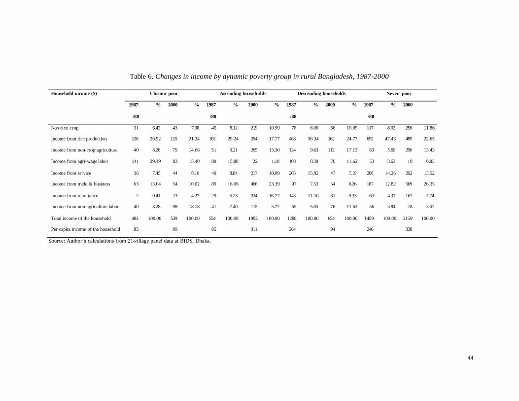
Second, the growth in household income was not uniform for all sources. The household

income from the non-agricultural sectors (defined broadly) has increased at a much faster rate

than from agricultural activity. As a result the share of agriculture in total household income

has decreased from 64 to 49 percent for the entire sample (Table 6). The decline was even

24

sharper for the ascending households as the matched share decreased from 63 to 43 percent.

The negative income growth observed for the rice sector was due to the adverse terms of

trade for this sector especially in the second half of the 1990s. However, it is striking that

average income from the rice sector has doubled for the ascending households group between

the two surveys. This is because the average rice acreage expanded by 70 percent for this

group. The acreage expansion combined with the switch to MV technology have helped them

to overcome the negative terms of trade effects arising from falling rice prices.28

Third, agricultural diversification promises to be an important source of future rural income

growth and poverty reduction. For the entire sample, income from the cultivation of non-rice

crops returned an annual growth of 6.4 percent, while that for non-crop agriculture (inclusive

of livestock and fisheries) was 8 percent. Agricultural diversification played an important role

in facilitating the escape from poverty on the part of the ascending households group. Thus,

for the latter, the average non-rice crop income increased by 12.6 percent per year, while

income from non-crop agriculture increased by 13.2 percent. These are impressive rates of

expansion notwithstanding the initial low base. As a result of the high growth the combined

share of these sources of income has increased by 7 percent even though the aggregate share

of agriculture has gone down (Table 6).

Fourth, as mentioned earlier, the strongest impetus to growth for the ascending households

and the never poor came from the non-agricultural sectors especially from trade, service, and

migration (remittances). These activities require higher access to human capital and financial

assets in which these two groups had a clear edge over the rest, as discussed earlier. Of

particular importance for the ascending households group was the income from trade and

25

business the share of which has increased from 16 to 23 percent, and remittances whose share

has gone up from 5 to 17 percent over the period.

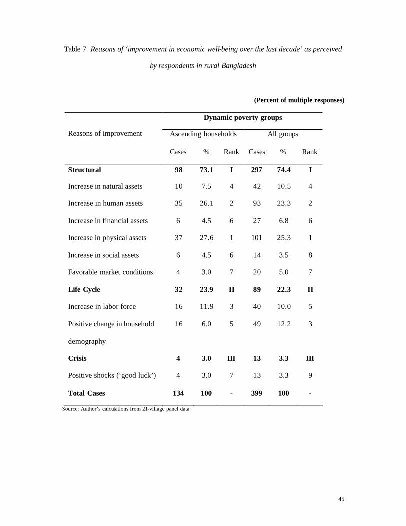
(h) Self -perceptions of the major ‘drivers of escape’

Households were asked to self-report the causes of their poverty dynamics over the past

decade. These self-perceived causes can be analysed in the livelihood framework to shed

further light on the drivers of changes in well-being during the inter-survey period.29 Table 7

presents results for all households reporting improvement as well as for the category of the

ascending households who actually moved out of poverty during the period. The results are

broadly in line with the preceding discussion. In addition, the household perceptions about

change can be used as weights to rank the importance of various factors influencing

livelihood outcomes. Households themselves have singled out several factors as the major

drivers of progress (see Annex 1 for the details of the household level self-reported causes of

improvement). Here we discuss the results for the ascending households only.

[Table 7 here]

Improvements in physical assets and human assets have been identified as the two most

important factors influencing the escape from poverty. They account for 28 and 26 percent of

the multiple responses, respectively. The process of ascendancy has been facilitated by

favorable change in household demography leading to the increased number of workers and

reduced number of dependents. The combined weight of these two factors is 24 percent.

26

Accumulation of natural assets, such as land, figured in 8 percent of cases was also cited as

an important driver of upward mobility.

6. EXPLAINING DESCENTS INTO POVERTY

Our knowledge of the factors influencing household’s sliding into poverty is much greater

than from ‘one off’ survey data. From Tables 5 and 6, one can construct a statistical picture

of the descending households category. First, changes in household demography have been

unfavorable for the group as a whole. Although the number of workers has increased, the

average family size has expanded even more. As a result, the proportion of labor force has

dropped from 36 to 27 percent during the period. Second, this group of rural households was

less successful in diversifying into more productive non-agricultural activities. Although the

share of non-farm workers has increased from 45 to 65 percent, the resultant outcome was

much less pronounced compared with the shifts recorded for the never poor and the

ascending households category. Third, the descending households group also lagged behind

in the development of human assets. Fourth, there was a general decline in the natural and

financial asset base for this group. The average land owned declined from 0.60 to 0.47 ha,

while credit access decreased from US$ 46 to 16 during this period. The average amount of

physical assets registered only a marginal increase of 6 percent over the entire period

compared with the very sharp accumulation recorded for the ascending households and never

poor groups. Fifth, the shrinking asset base has led to declining income earning pote ntials, as

evidenced from the comparison of income by sources between the two periods for the

descending households group. Except for income from non-agricultural labor the average

income derived from all other sources of household livelihood has declined in real terms.

27

What explains the descent of these households into poverty? The main factors, as perceived

by the households themselves, can be classified into three groups: ‘crisis’ factors, ‘lifecycle’

factors, and ‘structural’ factors (see Annex 2 for details). Crisis factors include natural

disasters, health-hazards, ‘personal insecurity’ and isolated ‘idiosyncratic’ events such as

social ceremonies. Lifecycle factors include an increase in the number of dependants and

splitting up of families reducing the number of earners. Structural factors include, for

example, erosion of the asset base such as alienation of land, lack of access to credit, loss in

business, and deteriorating market conditions for employment or income. The results are

presented in Table 8 for all households reporting deterioration over the last decade as well as

for the descending households group, which is our key interest here.

[Table 8 here]

The key causes of downward mobility for the descending households category were crisis

(discrete shocks) related factors in 38 percent of cases. Unfavorable lifecycle factors, such as

increase in the number of dependents and/or decrease in the number of earners, were the

second most important factor underlying retrogression in household fortunes, being singled

out in 35 percent of cases. Structural factors also cannot be discounted, being relevant in 27

percent of cases. A more disaggregated breakdown shows the importance of ill-health shocks

as the second most important factor of downward mobility (right after the factor of

unfavorable changes in household demography). Such shocks were reported in 18 percent of

cases. The loss of natural assets such as cultivable land—which was rated as important as the

health shocks – may be an outcome of adverse adjustments on the part of these households to

changing economic and social circumstances. Shocks related to natural disaster came next in

28

the order of importance, being present in 15 percent of cases, implying the possible presence

of spatial (village-level) dimension in the process of descent. These shocks include a range of

vulnerabilities such as loss of land due to river erosion, bad yield due to drought and

flooding, and damage of household assets.

7. CONCLUSIONS

The story of escapes from poverty based on the panel data—as typified by the experience of

the ‘ascending households’ category—confirms the general findings in the literature about

the importance of multiple routes for poverty reduction. What the panel data also point out is

that combining different exit routes is critical for the escape from poverty and that not all

poverty groups manage to combine these routes. This failure to combine routes is attributable

to the high initial level of poverty itself (as in the case of chronic poor) or because of adverse

turns and twists in economic and social circumstances (as in the case of descending

households). In this paper only the category of the ascending households—considered as a

group--demonstrated the ability to integrate various anti-poverty strategies, resulting in

relatively high savings-investment and income growth rate. These strategies included

relatively fast accumulation of different assets especially human and physical assets,

diversification of the asset base favoring relatively higher income -yielding non-agricultural

assets, a general re-orientation from agricultural activities to non-agricultural activities in

occupational choice and in the pooling of household incomes from different sources. This

does not undermine the importance of agriculture as the source of livelihood. Indeed, within

the generally declining share of agricultural sector (broadly defined) the ascending

households group showed dynamism in terms of adopting MV rice technology combining

this with greater emphasis on the cultivation of high value-added non-rice crops as well as

non-crop agriculture such as poultry, livestock, and fisheries. Access to human capital and

29

financial capital facilitated the transition from agricultural to non-agricultural activities, and

within agriculture, encouraged diversification into non-rice agriculture. This group also

actively used migration as a key livelihood strategy as remittance became an increasingly

influential aid to their struggle to climb out of poverty. In short, the success of the ascending

households category lies in pursuing a strategy of combining multiple routes of anti-poverty

and in exploiting the complementarities and synergies that exist among these diverse

livelihood approaches.30

The results for those slipping into poverty are based on the analysis of the ‘descending

households’. They do not represent the mirror image of the results derived for the upward

movements out of poverty. Thus, ‘structural’ factors related to the asset base of the household

and market conditions were seen as the drivers of change for the ascending households group,

being relevant in as high as 73 percent of cases. In contrast, the causes of downfall seem to

have diverse origins where ‘non-structural factors’ played a much more pronounced role. It is

the income shocks arising principally from ill-health and natural disaster that emerged

prominently among the lead self-reported causes of declining household fortunes. Favorable

and unfavorable confluence of life cycle factors rank second in both upward and downward

movements, respectively, though their effects are stronger in the case of descent than in

facilitating ascent from poverty.

Combinations of structural, lifecycle, and crisis factors may provoke either transient poverty

or chronic poverty–largely depending on the initial circumstances of the household. Thus for

households that have sufficient assets the death of the principal earning member or a poor

harvest may result in transient poverty. For those with nothing to fall back on the same

30

events can lead to chronic poverty. Available data do not allow us, however, to isolate these

two groups with differential poverty futures within the descending households category.

To what extent do the individual attributes of the ascending households make the ultimate

difference influencing them to pursue a path exploiting emerging rural opportunities better

and earlier than the other poverty groups? Was it because of an ‘entrepreneurship’ factor, a

certain ‘thriftiness’ in the character, or because of ‘high aspirations to catch up with the rich’,

or some other unobserved individual aspects?31 Or, was it simply the factor of being in the

‘right place at the right time with right kind of ideas’—a happy confluence of favorable

circumstances that led to the differing response patterns? In short, was it a matter of ‘good

luck’ or ‘good choice’—a unique (non-replicable) or universal (replicable) story of upward

mobility? These moments of life history cannot be fully captured through the available

quantitative panel data. Addressing these questions requires another kind of narrative, another

way of story telling, based on in-depth case studies and qualitative probing—a task we leave

for further research. Whatever, this study provides further confirmation that there has been

considerable progress in reducing poverty in Bangladesh in recent times. 32

31

References

Adnan, S. et al. (1977). Differentiation and Class Structure in Village Shamraj , Working

Paper No. 8, Village Study Group, Dhaka.

Ahmed, S. (2000). Bangladesh since Independence: Development Performance, Constraints

and Challenges, World Bank, Washington, D.C (Processed).

Alamgir, M. (1978). Bangladesh: A Case of Below Poverty Level Equilibrium Trap, BIDS,

Dhaka.

Alesina, A., & Rodrik, D. (1994). “Distributive Politics and Economic Growth”, Quarterly

Journal of Economics, Vol. 108, pp. 465-490.

Bakht, Z., & Shah, S. Eds. (1996). “Rural Non-Farm Development in Bangladesh”,

Bangladesh Development Studies, Vol. 24, Nos. 3 & 4.

BBS (2001). Preliminary Report of Household Income and Expenditure Survey 2000,

Bangladesh Bureau of Statistics, Dhaka.

Banerjee, A.V., & Newman, A. (1993). “Occupational Choice and the Process of

Development”, Journal of Political Economy, Vol. 101, pp. 274-298.

32

Bertocci, P.J. (1970). Elusive Villages: Social Structure and Community Organization in the

Rural East Pakistan, Unpublished Ph.D Thesis, Michigan State University, East Lansing,

Michigan.

BIDS (2001). Fighting Human Poverty: Bangladesh Human Development Report 2000,

Bangladesh Institute of Development Studies/ Planning Commission, Dhaka.

Bird, K., Hulme, D., Moore, K., & Shepherd, A. (2002). Chronic Poverty and Remote Rural

Areas, CPRC Working Paper 13, Institute for Development Policy and Management,

University of Manchester.

Boyce, J.K. (1987). Agrarian Impasse in Bengal: Institutional Constraints to Technological

Change, New York, Oxford University Press.

Carter, M.R., & May, J. (2001). “One kind of Freedom: Poverty Dynamics in Post-Apartheid

South Africa”, World Development, Vol. 29, No. 12, pp. 1987-2006.

CPD (2001). Citizen Task Force Report on Poverty , Centre for Policy Dialogue, Dhaka,

August (Processed).

De Vylder, S. (1982). Agriculture in Chains—Bangladesh, London, Zed Books.

Ellis, F. (2000). Rural Livelihoods and Diversity in Developing Countries, Oxford: Oxford

University Press.

33

Faaland, J., & Parkinson, J.R. (1975). Bangladesh: The Test Case of Development, University

Press Limited, Dhaka.

Foster, J., Green, J., & Thorbecke, E. (1984). ‘A Class of Decomposable Poverty Measures’,

Econometrica 52, 761-765.

Franda, M.F. (1982). Bangladesh-The First Decade, New Delhi, South Asian Publishers.

Galor, O., & Zeira, J. (1993). “Income Distribution and Macroeconomics”, Review of

Economic Studies, Vol. 60, pp. 35-52.

GoB (1991). “Poverty Alleviation” in Report of the Task Forces on Bangladesh Development

Strategies for the 1990s, Vol. 1, University Press Ltd., Dhaka.

GoB (2002). Bangladesh. A National Strategy for Economic Growth and Poverty Reduction,

Economic Relations Division, Ministry of Finance, Govt. of Bangladesh, April.

Hartmann, B., & Boyce, J. K. (1983). A Quiet Violence: View from a Bangladesh Village ,

London, Zed Books.

Hossain M., Sen, B., & Rahman, H. Z. (2000). “Growth and Distribution of Rural Income in

Bangladesh”, Economic and Political Weekly, Vol. 35, Nos. 52-53.

Hossain, M. & Sen, B. (1992). "Rural Poverty in Bangladesh: Trends and Determinants", Asian

Development Review, Vol. 10, No. 1.

34

Hossain, M., Bose, M. L., Chowdhury, A., & Meinzen-Dick, R. (2002). “Changes in

Agrarian Relations and Livelihoods in Rural Bangladesh” in V.K. Ramachandran and

Swaminathan, M. (eds), Agrarian Studies: Essays on Agrarian Relations in Less-Developed

Countries. Proceedings of the International Conference on “Agrarian Relations and Rural

Development in Less-Developed Countries”, 3-6 January 2002, Kolkata, India: Tulika Books.

Hulme, D., Moore, K., & Shepherd, A. (2001). Chronic Poverty: Meanings and Analytical

Frameworks, CPRC Working Paper 2, Institute for Development Policy and Management,

University of Manchester.

Huq, M.A. (1976). Exploitation and the Rural Poor: A Working Paper on the Rural Power

Structure in Bangladesh, Bangladesh Academy for Rural Development, Kotbari, Comilla.

Jack, J.C. (1916). The Economic Life of a Bengal District: A Study (Reprint: Oxford

University Press, 1975, with an introduction by Shahid Amin).

Jalan, J., & Ravallion, M. (2000). “Is Transient Poverty Different? Evidence for Rural

China”, Journal of Development Studies, 36/6, 82-99.

Jannuzi, F.T., & Peach, J.T. (1980). The Agrarian Structure of Bangladesh: An Impediment

to Development. Boulder, Westview Press.

Maloney, C. (1988). Behavior and Poverty in Bangladesh, University Press Ltd, Dhaka.

35

Moore, K. (2001). Frameworks for Understanding the Intergenerational Transmission of

Poverty and Well-being in Developing Countries , CPRC Working Paper 8, International

Development Department, School of Public Policy, University of Birmingham, Birmingham.

Morduch, J. (1995). “Income Smoothing and Consumption Smoothing”, Journal of Economic

Perspectives, 9, 103-114.

Mukherjee, R. (1971). Six Villages of Bengal, Popular Prakashan, Bombay.

Okidi, J., & Mugambe, G.K. (2002). An Overview of Chronic Poverty and Development

Policy in Uganda, CPRC Working paper 11, IDPM, University of Manchester.

Perotti, R. (1992). “Income Distribution, Politics, and Growth”, American Economic Review,

Vol. 82, pp. 311-316.

Persson, T., & Tabellini, G. (1994). “Is Inequality Harmful for Growth?”, American

Economic Review, Vol. 84, pp. 600-621.

Pradhan, M., & Ravallion, M. (2000). “Measuring Poverty Using Qualitative Perceptions of

Consumption Adequacy”, Review of Economics and Statistics, Vol. 82, No. 3.

Rafi, M., & Mushtaque, A., Chowdhury, R. (eds.) (2000). Counting the Hills: Assessing

Development in Chittagong Hill Tracts, University Press Ltd., Dhaka.

Ray, D. (1999). Development Economics, Oxford University Press, India.

36

Ravallion, M., & Sen, B. (1996). “When Method Matters: Monitoring Poverty in

Bangladesh”, Economic Development and Cultural Change , 44: 761-792.

Sen, B. (1996). “Explaining Movement in and out of Poverty” in H.Z. Rahman, M. Hossain,

and B. Sen (eds.), 1987-94: Dynamics of Rural Poverty in Bangladesh, Bangladesh Institute

of Development Studies (BIDS), Dhaka (Mimeo).

Sen, B., & Begum, S. (1998). Methodology for Identifying the Poorest at Local Level, WHO

Technical Paper No. 27, “Macroeconomics, Health and Development” Series, Geneva.

Sen, B. (2001). “Rethinking Anti-Poverty” in Changes and Challenges. A Review of

Bangladesh’s Development 2000, Centre for Policy Dialogue/ University Press Ltd.

Siddiqui, K. (2000). Jagatpur: 1977-97. Poverty and Social Change in Rural Bangladesh,

University Press Ltd, Dhaka.

Sobhan, R. (1982). The Crisis of External Dependence: The Political Economy of Foreign

Aid to Bangladesh, University Press Limited, Dhaka.

Sobhan, R. (ed.) (1991). The Decade of Stagnation: the State of the Bangladesh Economy in the

1980s, University Press Ltd., Dhaka, 1991, pp. 16-29.

Stern, N.H. (2002). The Investment Climate, Governance, and Inclusion in Bangladesh,

Public Lecture given at the Bangladesh Economic Association, Dhaka (Processed).

37

Thorp, J.P. (1978). Power among the Farmers of Daripalla: A Bangladesh Village Study ,

Caritas Bangladesh, Dacca.

Westergaard, K. (1978). “Mode of Production in Agriculture: A Bangladesh Village Study”,

Journal of Social Studies, Vol. 2.

Westergaard, K., & Hossain, A. (2000). ‘Boringram Revisited: How to Live Better on Less

Land’ in R. Jahan (ed.) Bangladesh: Promise and Performance, University Press Ltd, Dhaka.

World Bank (2000). World Development Report 2000/2001: Attacking Poverty , World Bank,

Washington, D.C. (published by Oxford University Press Ltd).

World Bank (2001). Poverty: Trends in Bangladesh during the Nineties, Background Paper

No. 1, Washington, D.C.

Van, Schendel, W. (1981). Peasant Mobility: The Odds of Life in Rural Bangladesh, Assen,

Van Gorcum and Humanities Press, Atlantic Highlands, New Jersey.

38

Table 1. Trends in poverty in Bangladesh: Consumption expenditure data

1983/84 1988/89 1991/92 2000

Rural

H 53.8 49.7 52.9 43.6

P(1) 15.0 13.1 14.6 11.3

P(2) 5.9 4.8 5.6 4.0

Urban

H 40.9 35.9 33.6 26.4

P(1) 11.4 8.7 8.4 6.7

P(2) 4.4 2.8 2.8 2.3

National

H 52.3 47.8 49.7 39.8

P(1) 14.5 12.5 13.6 10.3

P(2) 5.7 4.6 5.1 3.6

Notes:

1 The estimates for 1983/84 through 1991/92 are taken from Ravallion and Sen (1996) while that of 2000 are

author's estimates. National poverty estimates are population-weighted poverty measures obtained separately for rural

and urban sectors. The rural population shares are 88.7% (1983/84), 86.6% (1988/89), 83.4% (1991/92) and 78%

(2000). These measures use mean consumption expenditure as reported in Table 2.03 in successive HES reports, and

are based on the suitable parameterized Lorenz curve as estimated from the grouped distribution data ranked by per

capita consumption expenditure. The above estimates use the 1983/84 non-food poverty line as the base-year non-

food poverty line.

2 H is headcount measure, P(1) is poverty gap and P(2) is squared poverty gap.

39

Table 2. Summary statistics on growth and inequality in Bangladesh: Consumption data

Poverty line

taka/month/person

Survey

mean

taka/month/person

Mean/poverty

line (%)

Gini index

Urban:

1983/84 301.72 396.53 131 29.8

1988/89 453.65 695.19 153 32.6

1991/92 534.99 817.12 153 31.9

2000 724.56 1430.12 197 37.9

Rural:

1983/84 268.92 284.84 106 24.6

1988/89 379.08 435.39 115 26.5

1991/92 469.13 509.67 109 25.5

2000 634.48 820.20 129 29.7

Source: See note to Table 1.

40

Table 3. Slipping in and out of poverty by objective and subjective poverty lines in rural

Bangladesh, 1987/88 – 2000

Objective Poverty Line Subjective Poverty Line

Non-poor Poor Total Non-poor Poor Total

2000 2000 2000 2000

Non-poor 95 67 162 112 66 178

1987/88 (25.1) (17.7) (42.8) (30.0) (17.4) (47.4)

Poor 98 119 217 103 98 201

1987/88 (25.8) (31.4) (57.2) (27.2) (25.4) (52.6)

Total 193 186 379 215 164 379

(50.0) (49.1) (100) (56.7) (43.3) (100)

Source: Primary data at BIDS

41

Table 4. Incidence of chronic and transitory income poverty by land-poverty status:

21-Village panel data for 1987/88 and 2000

Objective Poverty Line

Exit

Ratio*

Vulnerability

Ratio**

never

poor

ascending

househol

ds

descending

households

chronic

poor

total

Land

poverty

status

1987/88

(1) (2) (3) (4) (5) (6) (7)

Poor ( up to

0.2 ha)

23

(14.4)

43

(27.0)

26

(16.4)

67

(42.2)

159

(100.0)

39.1 53.1

Vulnerable

(0.21 to 1 ha)

30

(22.1)

41

(30.1)

21

(15.4)

44

(32.4)

136

(100.0)

48.2 41.2

Non-poor

(1.01 and

above)

42

(50.0

14

(16.7)

20

(23.8)

8

(9.5)

84

(100.0)

63.4 32.3

All 95

(25.1)

98

(25.7)

67

(17.7)

119

(31.6)

379

(100.0)

45.2 41.4

Note: * Col. 6= Col. 2/ (Col.2+Col.4). ** Col. 7= Col. 3/ (Col. 1+Col. 3).

Source: Primary data at BIDS

42

Table 5. Asset base and income by dynamic poverty group in rural Bangladesh, 1987-2000

Chronic poor Ascending households Descending households Never poor Variables

1987/88 2000 1987/88 2000 1987/88 2000 1987/88 2000

Labor Force

Family size 5.66 6.05 6.50 6.40 4.88 6.97 5.94 6.39

Number of earners 1.54 1.77 1.70 2.31 1.75 1.87 1.75 2.18

No. of agricultural workers 1.19 1.10 1.05 1.01 1.30 1.22 1.12 0.84

No. of non-agricultural workers 0.35 0.67 0.65 1.30 0.45 0.65 0.63 1.34

Natural Assets

Owned land (ha) .27 .24 .42 .74 .60 .47 1.23 1.29

Cultivated land (ha) .27 .21 .38 .54 .78 .31 1.06 .75

Rice area (ha) .35 .29 .46 .78 1.01 .37 1.51 1.01

MV rice cultivated area (ha) .10 .18 .19 .57 .31 .24 .57 .70

Human Assets

Average years of schooling of all earners 3.16 5.90 5.18 12.60 4.08 7.45 8.09 15.98

Financial Assets ($)

Amount of institutional loan taken 13 31 17 45 15 12 13 108

Amount of non-institutional loan taken 27 10 28 17 31 4 89 42

Total amount of loan taken 40 41 45 62 46 16 102 151

43

Physical Assets ($)

Total non-land fixed assets 98 131 137 658 163 174 323 1242

Agricultural assets 77 101 123 213 154 99 298 268

Non-agricultural assets 20 30 14 445 9 75 25 974

Source: Author’s calculations from 21-village panel data at BIDS, Dhaka.

44

Table 6. Changes in income by dynamic poverty group in rural Bangladesh, 1987-2000

Chronic poor Ascending households Descending households Never poor Household income ($)

1987

/88

% 2000 % 1987

/88

% 2000 % 1987

/88

% 2000 % 1987

/88

% 2000

Non -rice crop 31 6.42 43 7.98 45 8.12 219 10.99 78 6.06 66 10.09 117 8.02 256 11.86

Income from rice production 130 26.92 115 21.34 162 29.24 354 17.77 468 36.34 162 24.77 692 47.43 489 22.65

Income from non-crop agriculture 40 8.28 79 14.66 51 9.21 265 13.30 124 9.63 112 17.13 83 5.69 290 13.43

Income from agri-wage labor 141 29.19 83 15.40 88 15.88 22 1.10 108 8.39 76 11.62 53 3.63 18 0.83

Income from service 36 7.45 44 8.16 49 8.84 217 10.89 205 15.92 47 7.19 208 14.26 292 13.52

Income from trade & business 63 13.04 54 10.02 89 16.06 466 23.39 97 7.53 54 8.26 187 12.82 569 26.35

Income from remittance 2 0.41 23 4.27 29 5.23 334 16.77 143 11.10 61 9.33 63 4.32 167 7.74

Income from non-agriculture labor 40 8.28 98 18.18 41 7.40 115 5.77 65 5.05 76 11.62 56 3.84 78 3.61

Total income of the household 483 100.00 539 100.00 554 100.00 1992 100.00 1288 100.00 654 100.00 1459 100.00 2159 100.00

Per capita income of the household 85 89 85 311 264 94 246 338

Source: Author’s calculations from 21-village panel data at BIDS, Dhaka.

45

Table 7. Reasons of ‘improvement in economic well-being over the last decade’ as perceived

by respondents in rural Bangladesh

(Percent of multiple responses)

Dynamic poverty groups

Ascending households All groups

Reasons of improvement

Cases % Rank Cases % Rank

Structural 98 73.1 I 297 74.4 I

Increase in natural assets 10 7.5 4 42 10.5 4

Increase in human assets 35 26.1 2 93 23.3 2

Increase in financial assets 6 4.5 6 27 6.8 6

Increase in physical assets 37 27.6 1 101 25.3 1

Increase in social assets 6 4.5 6 14 3.5 8

Favorable market conditions 4 3.0 7 20 5.0 7

Life Cycle 32 23.9 II 89 22.3 II

Increase in labor force 16 11.9 3 40 10.0 5

Positive change in household

demography

16 6.0 5 49 12.2 3

Crisis 4 3.0 III 13 3.3 III

Positive shocks (‘good luck’) 4 3.0 7 13 3.3 9

Total Cases 134 100 - 399 100 -

Source: Author’s calculations from 21-village panel data.

46

Table 8. Reasons of ‘deterioration in economic well-being over the last decade’ as perceived

by respondents in rural Bangladesh

(Percent of multiple responses)

Dynamic poverty groups

Descending

households

All groups

Reasons of deterioration

Cases % Rank Cases % Rank

Structural 25 26.6 III 92 31.4 III

Loss of natural assets 17 18.1 2 58 19.7 2

Loss of human assets - - - 3 1.0 9

Loss of financial assets 8 8.5 4 21 7.2 5

Loss of social assets - - - 2 0.7 10

Adverse market conditions - - - 8 2.7 8

Life cycle 33 35.1 II 98 33.4 II

Negative change in household

demography

33 35.1 1 98 33.4 1

Crisis 36 38.2 I 104 35.2 I

Ill-health 17 18.1 2 54 18.4 3

Natural disaster 14 14.9 3 24 8.2 4

Personal insecurity 3 3.2 5 11 3.7 7

Social ceremony 2 2.0 6 15 5.1 6

Total cases 94 100 - 293 100 -

Source: Author’s calculations from 21-village panel data.

47

Annex 1: Reasons for improvement as perceived by rural households in Bangladesh,

1987-2000

Factors of upward

mobility

Reasons for improving household economy

Structural

Natural assets • Sufficient amount of land/amount of land has increased

• Income has increased through sharecropping/leasing of land

• Income has increased through catching and selling of fish

Human assets • Family members are/were working in foreign countries

• Family members have/had services within the country

• Household head is industrious

• Promotion in service/increase in salary

Financial assets • Frugal

• Received pension/service benefits

• Received credit from Bank/NGO

Physical assets • The family has business

• Livestock rearing/milk production/poultry raising

• There are available bullocks for ploughing

• Income from tractors/ power tillers

• Income through cottage industry

• Increase in crop production

• Increased production as a result of cultivation of HYV

Social assets • A good relationship exists among all in the family

• Cooperation of relatives/others

Market conditions • There is good income from driving rickshaw/auto-rickshaw/tempo

• Income has increased by doing work as day laborer/other work

48

• Income from carpentry

Life Cycle

Labor force • Able members in the family and sons cooperate in work

• Earlier couldn’t work, now can

Household demography • Family size is small

• Expenditure is less relative to income in the family (because of

implied decrease of dependents)

• Less infirmity among the family members

Idiosyncratic

Positive income gains (good

luck)

• ‘God’s blessings’ on the family

49

Annex 2: Reasons for deterioration as perceived by rural households in Bangladesh,

1987-2000

Factors of downward

mobility

Reasons for deteriorating household economy

Structural

Natural assets • Land has decreased/was sold/mortgaged out

Human assets • Retired from service

Financial assets • Expenditure on children’s education is quite high

• Big expenditure for sending the son to foreign country

• Loss in business

• Increase in prices of agricultural inputs/implements

• There had been big expenditure for construction of houses

• Entangled in loan/repayment of loan

Social assets • Lack of discipline in the family

Market conditions • Son is unemployed/decreased job opportunity

• Low price of crop produced

Life Cycle

Household demography • Increase in number of family members

• Sons have separated

• Only one earning member in the family

• Number of earning members in the family is small

• Returning to father’s house after being abandoned by husband

• Expenditure is more than income (because of implied increase of

dependents)

50

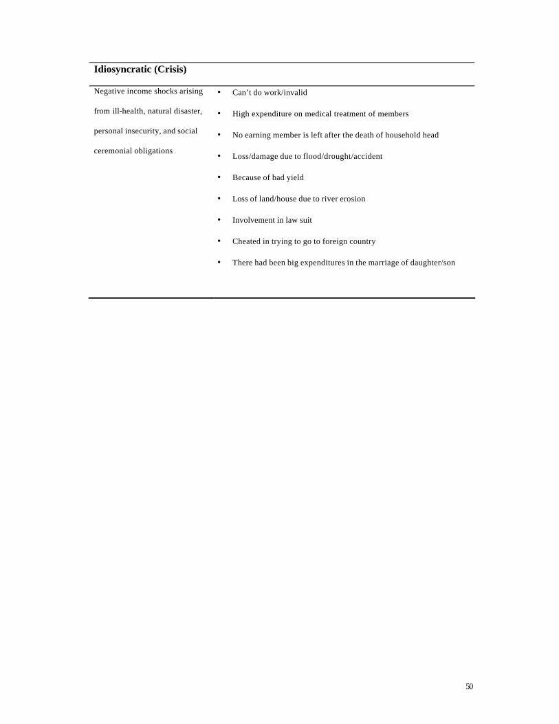
Idiosyncratic (Crisis)

Negative income shocks arising

from ill-health, natural disaster,

personal insecurity, and social

ceremonial obligations

• Can’t do work/invalid

• High expenditure on medical treatment of members

• No earning member is left after the death of household head

• Loss/damage due to flood/drought/accident

• Because of bad yield

• Loss of land/house due to river erosion

• Involvement in law suit

• Cheated in trying to go to foreign country

• There had been big expenditures in the marriage of daughter/son

51

NOTES

1 These 21 villages are a sub-set of a 32-village survey conducted by IRRI in 1987/88 and 2000. For a detailed

discussion of the initial sampling of the households and survey methodology, see Hossain et al (2002).

2 The density of population in Bangladesh is the highest in the world excluding Singapore. The estimated

population was 130 million in 2000 and population density 880 persons per sq km.

3 The terms ‘capital’ and ‘asset’ have been used interchangeably throughout the paper.

4 Consumption expenditure data have been used to estimate trends in income -poverty at the national level since

current consumption is considered to be a better indicator of permanent income status in the context of agrarian

society subject to year-to-year fluctuations in output.

5 Thus, annual per capita HIES consumption expenditure growth at national level, which was just 0.6 percent

during the period between 1983/84 and 1991/92, rose to 2.7 percent between 1991/92 and 2000. It may be noted

that the annual growth in per capita GDP was around 1.5 percent during the 1980s, but nearly doubled during the

1990s.

6A growing body of literature indicates that high initial income/ wealth inequality can dampen subsequent

economic growth and hence, the pace of income poverty reduction (see Ray, 1999).

7 Although t here are some notable studies on the ‘social’ aspects of stratification, mobility and deprivation in the

Bangladesh context they have not focused on the specific chronic poverty and/or chronic socially disadvantaged

groups. For the early treatment on the social aspects of change, see Mukherjee (1971) and Bertocci (1970),

which has been followed by a series of village study based investigations by Huq (1976), Adnan (1977), Thorp

(1978), Westergaard (1978), Maloney (1988), and, more recently, Siddiqui (2000), and Westergaard and Hossain

(2000). As regards ‘geographical poverty’ while the past studies such as GoB (1991) and BIDS (2001) have

identified the resource-poor areas through the ‘poverty mapping’ they stopped short of answering the central

52

question as to the social, economic, environmental, and political dimensions that inform continued spatial

divergence. Both these aspects will occupy a central place in future investigations.

8 Female-supported households include both de facto and de jure female-headed households as well as

households which draws mainly on the support of the female earners. The female-headed households per se is

not necessarily an indicator of severe poverty (depending on how absence of male is defined in the context

where absent males may be an important source of income).

9 Trends in real agricultural wages for casual daily laborers also support this conclusion. Thus, the nominal daily

agricultural wage rate has increased from 42 taka in 1991/92 to 51 taka in 1995/96, rising further to 64 taka by

2000. However, the real gains to agricultural laborers appear modest when deflated by the cost-of-living index

for the poor, as proxied by the rural poverty line. The extent of increase in real agricultural wages was only about

13 percent during the 1990s.

10 There is some doubt as to the quality of the urban module of the 1995/96 HIES data, indicating negative urban

consumption expenditure growth between 1995/96 and 2000. The quality of the rural module is not suspect.

11This is not to ignore the possibility that some rice-farming households did benefit even during the period of

falling rice prices. Thus, income from the rice sector was the second most important element of the rising fortune

of the ‘ascending households’ after ‘income from trade and business’. However, even for this group, the share of

income from the rice sector has declined from 29 to 18 percent between the two surveys, indicating the rising

relative importance of the non-rice, especially non-agricultural sectors in the 1990s (see, Table 6).

12 The ‘falling rice price story’ provides only a part-explanation of what has happened in the late 1990s. The

slower pace of rural poverty reduction is also partly attributable to the adverse impact of the 1998 flood, which

resulted in considerable physical assets depletion. It is possible that in 2000 many rural households were still

engaged in the “restoration and rehabilitation” phase in building up ‘lost assets’, thereby postponing increased

allocations for current consumption. Since the poverty estimates are based on the current consumption

expenditure data, the adverse impact of the 1998 flood may show up indirectly in the 2000 HIES (for similar

explanation, see World Bank 2001).

53

13 The panel results reported in this paper are based on the 379 ‘non-split’ households. The inclusion of ‘split’

households does not affect the main conclusions of the paper regarding the poverty ‘trends’ and the factors that

influenced the ‘dynamics of change’. However, the inclusion of the “split households” creates difficulties in

estimating changes in the asset base of the household crucial to the application of the livelihood framework

attempted in this paper. One empirical approach in the panel literature has been to integrate the split households

for the later year with the parent households for facilitating the ‘before -after’ comparison. This is not

theoretically compelling; indeed, it may be a better idea to discuss the case of the split households separately, as

done in the case of ‘missing’ households. Given the focus of the present paper on understanding the ‘drivers of

change’ with respect to those who escaped poverty and those who descended into poverty the exclusion of the

split households would not make a critical difference. The latter, of course, would be a relevant consideration in

estimating the levels of poverty based on the panel sample, which is not our main focus here.

14 The method is implemented in two stages, as the objective poverty line has two components. First, a costing of

the normative fixed bundle of 2112 calories is carried out, yielding a food-poverty line (for the bundle and the

method of costing see, Hossain and Sen 1992). Second, the average non-food expenditures typically incurred by

households located at the food-poverty line are considered “normative” non-food allowances. This gives the non-

food poverty line. Adding the two components one gets the total poverty line for the base year. The base year

poverty line is updated for the subsequent years by using a cost-of-living index constructed for the poor.

15 The idea of a subjective poverty line needs to be distinguished from the self-perception of households about

their poverty status. The idea here is to find a cut-off line of income, which would be corresponding to those

persisting at the food poverty line. The 2000 survey data collected information on the self-perception of

households about their relative well-being status (“how do you compare yourself with the other households in

the village?”). The survey also made a separate query as to “whether the households had adequate three meals a

day”. Combining these one could identify the households who have self-categorized themselves as poor yet had

adequate three meals a day. These households may be considered as households located at the food-poverty

threshold. The per capita total income of these households gives the norm of what is called here the ‘subjective

poverty line’. For a similar approach to defining a subjective poverty line, see Pradhan and Ravallion (2000).

54

16 Ideally, one would like to categorize the households into five ‘dynamic poverty‘ groups, as suggested by

Hulme et al (2001). These are (a) always poor, (b) usually poor, (c) churning poor, (d) occasionally poor, and (e)

never poor. With the two-period data we can identify the two polar categories of always poor and never poor.

However, identification of other ‘intermediate categories’ requires multiple period observations. In the

discussion that follows it is assumed that the poverty dynamic of a household is represented by a straight line

connecting its levels of poverty in 1987/88 and 2000. While such an assumption is undesirable data for

intermediate times is not available.

17 Here chronic poverty is defined in the ‘time’ dimension focusing on the durat ion in poverty. The longer the

duration, the greater the chronicity. The long duration of poverty in itself can be viewed as an aspect of ‘severity

of poverty’ as well. The tightest possible definition of chronic poverty would be intergenerationally transmitted

poverty (Moore 2001). A generation could be set at 15 years. From this angle one can interpret the results of the

21-village survey with a span of about 13 years providing the basis for computing intergenerational poverty.

Table 3 provides the upper bound value of the proportion of intergenerational poor around 31 percent.

18 The category of ‘descending households’ should not be readily equated to the term ‘transient poor’. This is

because a descent into poverty in many cases can have longer-term imp lications, as temporary shocks can lead to

permanent poverty traps (Morduch 1995).

19 A panel of 1,200 rural households studied by BIDS in 1990 and 1994, also revealed considerable movements

in and out of income poverty. About 38 percent of households stayed in poverty and 28 percent stayed above the

poverty line. The other 34 percent of cases, however, involved movements in and out: 17 percent of households

became new poor, while 18 percent escaped poverty (Sen 1996).

20 This has been noted elsewhere. See, for instance, Carter and May (2001) suggesting a measurement approach

integrating the ‘asset poverty line’ with the ‘income poverty line’. Okidi and Mugambe (2002) also explored

how poverty dynamics can differ depending on the “percentage deviation” of households from the income

poverty line.

21 These growth rates are calculated from Table 6.

55

22 This, of course, does not imply advocacy for a generalized menu of anti-poverty for all. Even if we know the

specific drivers that helped the ascending households in their past success, still a case can be made for special

(additional to the generalized menu) policy attention to the chronic poor. This may be required to ensure their

inclusion in the very activities that helped the ascending households earlier to c limb out of poverty.

23The rural livelihoods approach highlights the factor of initial distributive as well as accumulation conditions in

terms of diverse asset access/ endowments as a central factor influencing changes in the well-being. It also

underscores the need for analyzing the intervening ‘transformative’ institutional structures influencing the return

on assets. Both these factors combined together influence the livelihood outcomes. The livelihoods approach is

not uncontroversial, however, in the context of alternative views of the Marxist and “political economy” schools.

The approach does not adequately focus on the historical analysis of embedded power relations within which

long-run poverty dynamics are situated. The problem, however, is that the quantitative panel surveys typically

lack information on the relational aspects that are highlighted by these alternative schools. Given the nature of

poverty data-base available for Bangladesh to track down the changes during the decade of the 1990s we

considered the rural livelihoods framework as the most suitable approach to describe the process of transition in

the context of movement in and out of poverty. This is not to undermine the importance of other forms of

investigation into the process of poverty transitions. Van Schendel (1981), for instance, provides an application

of the historico-sociological approach to studying long-run household mobility based on repeat village studies.

The study of material conditions of the rural inhabitants in the district of Fardipur carried out by J.C. Jack (1916)

in the early part of 20th century represents a classic attempt to combine both quantitative and qualitative

investigations (for a discussion on Jack’s contribution to poverty analysis, see Sen and Begum 1998).

24 The term ‘social asset’ (or ‘social capital’) may be defined differently depending on the unit of observation.

While there is no consensus in the literature regarding the precise definition of the term it is useful to distinguish

three levels of social capital analysis. For a summary review, see World Bank (2000).

25 This appears to be a better alternative than using the series of consumer price index (CPI) published by the

BBS for the nineties, which appears to be a rather unreliable guide to the rate of rural inflation.

56

26 Do note that these figures are higher than those reported by Matin and Hulme (in this volume) who examine

the issue of microcredit in more detail.

27 Between the two agricultural censuses of 1983/84 and 1995/96 the total availability of agricultural land has

declined by about 1 million ha to meet the growing demand for non-agricultural use such as housing and

urbanization.

28 This possibility, however, demands further scrutiny.

29 For the purpose of the present discussion it is important to take note of the broad correlation that exists

between the subjective and objective ranking of well-being changes for the 21-village panel. Thus, about 64

percent of the ascending households have self-categorised themselves under the “improvement” group, while 57

percent of the descending households have self-classified themselves under the “deterioration” group. In short,

there is no one-to-one correspondence. There seems to be a considerable presence of ‘dissatisfied non-poor’

(who slipped out of objective poverty but still self -report their situation as deteriorating) and ‘satisfied poor’

(who descended further into objective poverty but still self -assess their changes in well-being in favorable

terms). Rather than consider these outcomes as outliers, or as mere noises in the data, one can analytically

separate out these deviations from the predicted response as a topic of further research under the possible theme

of ‘unhappiness and poverty’.

30 This does not necessarily imply that all of these strategies have to be present in the representative household

from the ascending households group. From the evidence assembled in the present paper it is clear that the

ascending households as a group employ a large range of livelihood strategies compared to the chronic poor and

descending households groups. Additional evidence not discussed in the paper points out that the incidence of

combination of multiple strategies is also more frequent in case of the ascending households than in other

groups. The dynamics of integration, especially with respect to the effective management of diverse portfolio of

assets as well as the time-use pattern, however, requires further investigation.

31 These qualities do matter in the process of poverty transitions, though typically have received marginal

attention in the Bangladesh literature. One notable exception is Maloney (1988).

57

32 This has been argued in greater details elsewhere based on macro -level social and economic data (see, Sen

2001; BIDS 2001; GoB 2002) and is gaining increasing international recognition (see, for instance, Ahmed

2000; Stern 2002).