Drivers of Digital Attention:Evidence from a Social Media Experiment*

Guy Aridor†

JOB MARKET PAPER

November 5, 2021; LATEST VERSION HERE

AbstractI study demand for social media services by conducting an experiment where I comprehen-

sively monitor how participants spend time on digital services. I shut off access to Instagram

or YouTube on their mobile phones and investigate how participants substitute their time allo-

cations during and after the restrictions. During the restriction period, I observe substitution

towards a wide range of alternatives including across product categories and off digital devices

and relate these findings to market definition in attention markets. Participants with the Insta-

gram restriction had their average daily Instagram usage decline after the restrictions are lifted.

Participants with the YouTube restriction spent more time on applications installed during the

restriction period both during and after the restriction period. Motivated by these results, I

estimate a discrete choice model of time usage with inertia and find that inertia explains a large

portion of the usage on these applications. I apply the estimates to conduct merger evaluation

between prominent social media applications using an Upward Pricing Pressure Test for atten-

tion markets. I find that inertia plays an important role in justifying blocking mergers between

the largest and smallest applications, indicating that digital addiction issues are important from

an antitrust perspective. Overall, my results highlight the usefulness of product unavailability

experiments in analysis of mergers between digital goods.

Keywords: Social Media, Attention Markets, Field Experiment, Consumer Demand, Mergers

JEL Codes: L00; L40; L86.

*I am indebted to my advisors Yeon-Koo Che, Tobias Salz, Andrey Simonov, and Michael Woodford for their guidance. I thank Maayan Malterfor partnering on the data collection. I thank Matt Backus, Mark Dean, Laura Doval, Garrett Johnson, Andrea Prat, Silvio Ravaioli, Pietro Tebaldi,and Xiao Xu for their valuable comments. I am grateful to Ro’ee Levy who provided advice on recruitment as well as to NYU, HKUST, andChicago Booth for providing access to their lab pools. I thank Tyler Redlitz and Rachel Samouha for excellent research assistance. The experimentwas approved by the Columbia University IRB as protocol AAAS7559. Finally, I thank the Columbia University Program for Economic Researchfor providing funding for this research.

†Columbia University, Department of Economics. Email: g.aridor@columbia.edu

1 Introduction

In the past two decades social media has evolved from a niche online tool for connecting withfriends to an essential aspect of people’s lives. Indeed, the most prominent social media applica-tions are now used by a majority of individuals around the world and these same applications aresome of the most valuable companies in the modern day.1 Due to the sheer amount of time spenton these applications and concentration of this usage on only a few large applications, there hasbeen a global push towards understanding whether and how to regulate these markets (Scott Mor-ton et al., 2019; CMA, 2020).2 At the heart of the issue is that consumers pay no monetary priceto use these applications, which renders the standard antitrust toolkit difficult to apply as the lackof prices complicates the measurement of demand and identification of plausible substitutes forthese applications.3 The demand measurement problem is further compounded by the fact thatsome fraction of usage may be driven by addiction to the applications or, more broadly, inertia(Hou et al., 2019; Morton and Dinielli, 2020). This facet of demand inflates the market share ofthese applications and makes it difficult to disentangle whether substitution between prominentapplications is due to habitual usage or direct substitutability. This decomposition is further infor-mative about whether policies aimed at curbing digital addiction are important from an antitrustperspective. These two complications together have led to substantial difficulties in understandingthe core aspects of consumer demand that are crucial for market evaluation and merger analysis.

In this paper I empirically study demand for these applications and illustrate how these findingscan be used for conducting merger evaluation in such markets. I conduct a field experiment where,using parental control software installed on their phone and a Chrome Extension installed on theircomputer, I continuously track how participants spend time on digital services for a period of 5weeks.4 I use the parental control software to shut off access to YouTube or Instagram on theirphones for a period ranging from one to two weeks. I explicitly design the experiment so that thereis variation in the length of the restriction period and continue to track how participants allocate

1For instance, Facebook, which owns several prominent social media and messaging applications, is the 6th mostvaluable company in the world with over a trillion dollars in market capitalization. Additionally, Twitter has a marketcapitalization of over 50 billion dollars and is in the top 500 highest valued companies in the world according tohttps://companiesmarketcap.com/ on August 30th, 2021.

2As pointed out by Prat and Valletti (2021), the increased concentration of consumer attention can have ramifica-tions far beyond this market alone since increased concentration in this market influences the ability for firms to enterinto product markets that rely on advertising for product discovery.

3This issue was at the heart of the Facebook-Instagram and Facebook-WhatsApp mergers. Without prices, regula-tory authorities resorted to market definitions that only focused on product characteristics, as opposed to substitutionpatterns of usage. For instance, Instagram’s relevant market was only photo-sharing applications and WhatsApp’s rel-evant market was only messaging applications. This issue continues to play a role in the ongoing FTC lawsuit againstFacebook where a similar debate is ongoing.

4This ensures that I have objective measures of time usage which is crucial for my study as subjective measuresof time spent on social media applications are known to be noisy and inaccurate (Ernala et al., 2020).

1

their time for two to three weeks following the restrictions. The time usage substitution patternsobserved during the restriction period allow me to observe plausible substitutes, despite the lackof prices. The extent to which there are persistent effects of the restrictions in the post-restrictionperiod allows me to uncover the role that inertia plays in driving demand for these applications.

I exploit the rich data and variation generated by the experiment to investigate aspects of de-mand related to competition policy and merger analysis. I provide an interpretation of the timesubstitution observed when the applications are restricted; this interpretation sheds light on rele-vant market definitions for the restricted applications – the set of applications that are consideredsubstitutable relative to the application of interest – which have played a prominent role in antitrustpolicy debates. I further use the experimental substitution patterns to determine whether there isevidence of “dynamic” elements of demand as well as important dimensions of preference hetero-geneity. Guided by these results, I estimate a discrete choice model of time usage with inertia toproduce an important measure of substitution that is crucial for merger analysis: diversion ratios.I provide estimates of diversion ratios both with and without inertia, disentangling the extent ofdiversion due to inertia versus inherent substitutability of the applications. In order to understandhow important inertia is for merger analysis, I apply the two sets of diversion ratio estimates toevaluate mergers between social media applications. One important policy interpretation of the noinertia counterfactual is to provide insight into how and whether policies aimed at curbing digi-tal addiction are important not just in their own right, but also in influencing usage and diversionbetween the applications to the extent that they would influence merger assessments.

Broader antitrust concerns motivate the following two questions about substitution patterns:what types of activities do participants substitute to and is this substitution concentrated on promi-nent applications or dispersed among the long tail? The most directly relevant question is whetheror not there is evidence that they substitute across application categories. This has featured promi-nently in debates between these applications and regulators since the degree to which applicationssuch as YouTube and Instagram are substitutable is important for monopolization claims aboutFacebook and mergers between different types of applications. Even if there is cross-categorysubstitution, then it is also important to understand to what extent this is concentrated towardspopular applications such as YouTube, within the vast Facebook ecosystem which spans applica-tion categories, or dispersed towards smaller applications competing with them. I argue that theset of applications that consumers substitute to during the restriction period serves as the broadestmarket definition since it measures consumer substitution at the “choke” price – the price which issufficiently high so that no one would use the application at all.5 Thus, even with zero consumer

5This is similar to the interpretation given to such experiments in Conlon and Mortimer (2018). Note that thevariation does not isolate the observed substitution to be about price exclusively. Indeed, one can broadly interpret thisas the substitution at the choke advertising load or application quality as well. This will lead to some nuance in thevalue of this variation in the demand model, but is not first-order for the relevant market definition exercise.

2

prices, the product unavailability variation alone allows me to assess the plausibility of claims thatapplications such as YouTube and Instagram directly compete against each other for consumertime.

In order to assess the extent of cross application category substitution, I manually pair eachobserved application in the data with the category it is assigned to on the Google Play Store. Forthe Instagram restriction group, I find a 22.4% increase in time spent on other social applications,but also a marginally significant 10.2% increase in time spent on communication applications.For the YouTube restriction group, I find that there is a null effect of substitution towards otherentertainment applications, but also find a 15.2% increase in time spent on social applications.While this provides evidence for cross-category substitution, there is a notable asymmetry whereblocking Instagram, a social media application, does not lead to substitution towards entertainmentapplications such as YouTube, whereas blocking YouTube, an entertainment application, leads tosubstitution towards social applications such as Instagram and Facebook.6 Pairing these resultswith the conservative relevant market definition test implies that market definitions ought to spanacross the application categories between which I observe substitution. I show that, under thismarket definition, concentration is meaningfully lower relative to only using application categoriesas the relevant market definition.

There are several nuances to the implications of the application category substitution on thedegree of market concentration. First, for both the YouTube and Instagram restriction, there isconsiderable substitution towards the outside option – off the phone.7 This indicates that, even if Iconsider substitutes across all the categories on the phone, participants were not able to find a viablesubstitute in any other application. The framing of the debate in terms of within versus acrosscategory substitution therefore is potentially misleading as this shift towards the outside optionimplies that both YouTube and Instagram have considerable market power. Second, a large part ofthis market concentration is due to Facebook’s joint ownership of Facebook, Instagram, Messenger,and WhatsApp; considering these as being independently owned applications substantially reducesthe degree of market concentration even more so than cross-category market definitions. Indeed,non-Instagram Facebook owned applications have a 17.9% increase in time spent for the Instagramrestriction group. Thus, some of the observed cross-category substitution is substitution within theFacebook ecosystem. Third, I elicit a subjective measure of how each participant uses the set ofprominent social media, entertainment, and communication applications and find that, especially

6This casts some subtlety to a debate in CMA (2020) between Facebook and regulators where Facebook usesoutages of YouTube to claim that they compete with them. My experimental results point to a similar result in responseto the YouTube restriction, but notably I observe an asymmetry where the reverse is not true during the Instagramrestriction. Indeed, for Instagram, there is more within category substitution relative to cross category substitution.

7Using the data from the weekly surveys and the Chrome Extension, I am able to conclude that only a smallfraction of this time is due to substitution to the restricted application on other devices.

3

for social media applications, participants use the applications for different reasons ranging fromsocial connection to pure entertainment. This points to the application categories not necessarilycapturing the different uses of these applications and partially explaining some of the observedcross-category substitution.

The experimental design further allows me to understand whether there are potentially dynamicelements associated with demand by assessing whether the restrictions modify post-restriction timeallocations on the restricted application as well as those substituted to during the restriction period.There are two possible channels through which the restrictions could impact post-restriction usage.The first possible channel is that the restriction could serve as a shock to participants’ habits anddepress usage after the restriction period. While I remain agnostic about the mechanism throughwhich this change would occur, one important descriptive statistic is that up to 51% of the par-ticipants in the study are psychologically addicted to social media according to the scale by An-dreassen et al. (2012) that participants complete in the baseline survey. Thus, the experiment couldserve as a shock to the addictive habits of the participants in the experiment. The second possiblechannel is intertemporal substitution whereby the restrictions lead participants to defer consump-tion until the restriction period is lifted. These two channels are not mutually exclusive and theaim is to assess which of these is first-order in modeling demand. This motivates why I design theexperiment so that the restriction lengths are relatively long and also varied in length as one mightexpect that these effects are more apparent the longer the restriction length is.

I explicitly test whether there is a spike in usage of the restricted application on the day thatit is no longer blocked for the participants and find no evidence of this for either the one or twoweek restriction group. I use this as evidence that the intertemporal substitution channel is notprominent as one would expect the built up usage during the restriction period to lead to a spikein usage when the application was returned. I find a consistent body of evidence that there is apersistent reduction in time spent on the restricted applications and that this is primarily drivenby the participants that had the two week restriction, but not those for the one week restriction.For the Instagram restriction, the two week restriction group reduced average daily usage relativeto the control group by 5 minutes and had a similar reduction relative to the one week restrictiongroup. Estimating quantile treatment effects indicates that this is mainly driven by the heaviestusers of the applications. A survey sent after the study indicates that this reduction in time spentpersists even a month following the conclusion of the study. For the YouTube restriction, thereis suggestive evidence of a similar difference between the one and two week restriction group,but the resulting difference in average daily usage is not statistically significant. However, I findthat participants in the YouTube restriction spent more time on applications installed during therestriction period relative to the control group and persisted to use these applications even in thepost-restriction period. I use both the persistent reduction in usage of Instagram and the increased

4

usage of applications installed during the restriction period of YouTube as evidence that inertiaplays a role in demand for these applications.

The experimental results shed light on aspects of demand required to understand the usage ofthese applications. However, in order to conduct merger analyses, an important output of a demandstudy is estimates of diversion ratios. The diversion ratio from application i to application j is de-fined as the fraction of sales / consumption that gets diverted from application i to application j as aresult of a change in price / quality / availability of application i. Diversion ratios provide a quanti-tative magnitude of substitution between two applications and are especially important for mergeranalysis as they play a prominent role in the current US horizontal merger guidelines for measur-ing possible unilateral effects. I estimate a discrete choice model of time usage between prominentsocial media and entertainment applications and use the estimates to compute second-choice di-version ratios – diversion with respect to a change in availability. I incorporate the insights fromthe experimental results directly into the demand model. I incorporate inertia by including pastusage into consumer utility similar to state-dependent demand estimation models (Dube, Hitschand Rossi, 2010; Bronnenberg, Dube and Gentzkow, 2012). Furthermore, I directly incorporatethe heterogeneity in subjective usage of the applications into the utility function in order to capturethe preference heterogeneity indicated by the experimental results and exploit the granular timeusage data that I collect in order to have a flexible outside option that varies across time.

The main counterfactual that I consider is to shut down the inertia channel and compute howthis impacts overall usage of the set of considered applications as well as the estimated diversionratios. I find that longer term inertia drives nearly 40% of overall usage of the considered appli-cations. This counterfactual further allows me to disentangle the extent to which the diversionbetween two applications is due to inherent substitutability as opposed to being driven by inertiaeffects. For instance, there is large observed diversion from Snapchat to Instagram, which couldbe due to Snapchat and Instagram being inherently substitutable applications or it could be dueto the fact that people are more likely to have built up habit stock of Instagram that induces themto be more likely to use it in the absence of Snapchat. However, it could also increase the con-verse diversion from Instagram to Snapchat since, for smaller applications, they are less likely tohave built up habit stock and may actually benefit from the lack of built up habit stock on largerapplications such as YouTube. The diversion estimates without inertia thus filter out the secondchannel and provide a more natural measure of substitution between these applications. While Iremain agnostic to the mechanism behind inertia, a large portion of the estimated inertia is likelyfrom addictive usage as indicated by the qualitative evidence accumulated throughout the study.Indeed, contemporaneous work by Allcott, Gentzkow and Song (2021) similarly shows that 31%of usage of these applications is driven by behavior consistent with rational addiction. Regulatorsaround the world are actively debating how to deal with digital addiction in its own right, whether

5

through directly regulating the time usage on the applications or indirectly regulating the curationalgorithms and feed designs used on these applications.8 Since my experiment does not preciselyisolate the extent to which usage is driven by addiction, one can consider the results here as anupper bound on how these policies would influence the subsequent diversion between these appli-cations and whether this channel is a sufficient driver of usage and diversion to influence mergerassessments.

I conclude the paper by applying the diversion ratios to hypothetical merger evaluations be-tween prominent social media and entertainment applications. I develop a version of the UpwardPricing Pressure test for attention markets where applications set advertising loads (i.e. number ofadvertisements per unit time) and advertisers’ willingness to pay depends on the time allocations ofconsumers. As is standard, I use the estimates of consumer diversion from my model, set a thresh-old on the efficiency gains in application quality arising from a merger, and determine whether amerger induces upward pressure on advertising loads. My formulation captures a unique aspectof online “attention” markets where additional consumer time on an application induces greaterability to target consumers and increases advertiser willingness to pay.

I find that, depending on how sensitive advertising prices are to time allocations, many merg-ers between prominent social media applications should be blocked with inertia, but many do notwithout inertia. The main intuition behind this is that with inertia the mergers that get blocked,such as Snapchat-YouTube, are due to the merged firm’s incentive to increase advertising loads onthe smaller application (Snapchat) in order to divert consumption towards the larger application(YouTube). When there is no inertia in usage, the diversion from the smaller to the larger appli-cation is lower since YouTube does not get the benefit of already being a popular application witha large amount of consumer habit stock built up. Thus, my results indicate that the role of inertiain inflating market shares and diversion ratios towards the largest applications is important for jus-tifying blocking mergers between the smaller and larger applications. This highlights how digitaladdiction issues are directly relevant to antitrust policy as they inflate the time usage and diversionbetween applications by a sufficient amount to lead to meaningfully different conclusions aboutmergers between these applications.

8There are bills proposed in the US Congress, such as the Kids Internet Design and Safety Act, https://www.congress.gov/116/bills/s3411/BILLS-116s3411is.pdf, aimed at regulating certain design featuresthat encourage excess usage and the Social Media Addiction Reduction Technology (SMART) Act, https://www.congress.gov/bill/116th-congress/senate-bill/2314/text, directly aiming to limit time spenton these applications. In the European Union the currently debated Digital Services Act has several stipulations on reg-ulating curation algorithms, https://digital-strategy.ec.europa.eu/en/policies/digital-services-act-package. In China, the government has explicitly set a time limit of 40 minutes on chil-dren’s usage of the popular social media application TikTok, https://www.bbc.com/news/technology-58625934. Furthermore, there is a constant stream of popular press articles focusing on additional proposals tolimit the addictive nature of these applications (e.g. see https://www.wsj.com/articles/how-to-fix-facebook-instagram-and-social-media-change-the-defaults-11634475600).

6

More broadly, this paper highlights the usefulness of product unavailability experiments fordemand and merger studies between digital goods. I exploit the insight that digital goods enableindividual level, randomized controlled experiments of product unavailability that are difficult toconduct with other types of goods and in other markets. These experiments enable causal es-timates of substitution patterns and identify plausible substitutes even when consumers pay noprices. Furthermore, they can be used to estimate the relevant portions of consumer demand thatare difficult to estimate using only observational data and are required for relevant market defini-tion and merger assessment. As a result, they serve as a practical and powerful tool for antitrustregulators in conducting merger assessments in digital markets.

The paper proceeds as follows. Section 2 surveys papers related to this work. Section 3 pro-vides a full description of the experiment and the resulting data that I collect during it. Section 4describes pertinent descriptive statistics of the data that are useful for understanding how partic-ipants spend their time and use the social media applications of interest. Section 5 documentsthe experimental results with respect to time substitution both during and after the restriction pe-riod. Section 6 develops and estimate the discrete choice time usage model with inertia. Section 7posits the Upward Pricing Pressure test that I use for hypothetical merger evaluation and applies itto mergers between prominent social media applications. Section 8 concludes the paper with somefinal remarks and summary of the results.

2 Related Work

This paper contributes to four separate strands of literature, which I detail below.

Economics of Social Media: The first is the literature that studies the economic impact of socialmedia. Methodologically my paper is closest to Allcott et al. (2020); Brynjolfsson, Collis and Eg-gers (2019); Mosquera et al. (2020) who measure the psychological and economic welfare effectsof social media usage through restricting access to services. Allcott et al. (2020); Mosquera et al.(2020) restrict access to Facebook and measure the causal impact of this restriction on a battery ofpsychological and political economy measures. Brynjolfsson, Collis and Eggers (2019) measuresthe consumer surplus gains from free digital services by asking participants how much they wouldhave to be paid in order to give up such services for a period of time. This paper utilizes a sim-ilar product unavailability experiment, but uses the product unavailability experiment in order tomeasure substitution patterns as opposed to quantifying welfare effects.

A concurrent paper that is also methodologically related is Allcott, Gentzkow and Song (2021).They utilize similar tools to do automated and continuous data collection of phone usage.9 They

9An important antecedent of this type of automated data collection is the “reality mining” concept of Eagle and

7

focus on identifying and quantifying the extent of digital addiction by having separate treatmentsto test for self-control issues and habit formation. I argue that my experimental design also enablesme to understand the persistent effects of the restriction, which I use to identify a demand model oftime usage with inertia. While my experiment does not allow me to identify the precise mechanismbehind this inertia effect, I rely on Allcott, Gentzkow and Song (2021) to argue that the most likelypossible mechanism is tied to digital addiction. Thus, I view Allcott, Gentzkow and Song (2021) asbeing complementary to my work as I focus on the competition aspect between these applications,but also find patterns consistent with their results.10

Finally, there is a burgeoning literature on the broader economic and social ramifications ofthe rise of social media applications. Collis and Eggers (2019) study the impact of limiting so-cial media usage to ten minutes a day on academic performance, well-being, and activities andobserves similar substitution between social media and communication applications. The broaderliterature has focused on political economy issues associated with social media (Bakshy, Messingand Adamic, 2015; Corrigan et al., 2018; Enikolopov, Makarin and Petrova, 2020; Levy, 2021) aswell as its psychological impact (Levy, 2016; Burke and Kraut, 2016; Kuss and Griffiths, 2017;Bailey et al., 2020; Baym, Wagman and Persaud, 2020).

Product Unavailability and State-Dependent Demand Estimation: The second is the literaturein marketing that studies brand loyalty and, more broadly, state-dependent demand estimation. Thediscrete choice model of time usage that I consider closely follows the formulation in this literaturewhere past consumption directly enters into the consumer utility function and the empirical chal-lenge is to disentangle the inertia portion of utility from preference heterogeneity (Shum, 2004;Dube, Hitsch and Rossi, 2010; Simonov et al., 2020). I consider that consumers have a habit stockthat enters directly into the utility function, which I interpret as inertia that drives usage of theapplications and is similar to the formulation in Bronnenberg, Dube and Gentzkow (2012).

Relative to this literature, I exploit the fact that I conduct an experiment and induce productunavailability variation as a shock to consumer habits in order to identify this portion of consumerutility. Conlon and Mortimer (2013, 2018); Conlon, Mortimer and Sarkis (2021) explore the valueof product unavailability in identifying components of consumer demand. In this paper my focus

Pentland (2006) who first used mobile phones to comprehensively digitize activities done by experimental participantsand, at least for the author, served as an important point of inspiration. One further point worth noting is that the studydone by Allcott, Gentzkow and Song (2021) relies on a custom-made application, whereas the primary data collectiondone in my paper relies on a (relatively) cheap, publicly available, parental control application and an open sourceChrome extension which is more accessible to other researchers. Furthermore, Allcott, Gentzkow and Song (2021)are only able to comprehensively track participants on smartphones, whereas I can additionally comprehensively tracksubstitution towards other devices without having to rely on self-reported data.

10In the theory literature, Ichihashi and Kim (2021) study competition between addictive platforms where platformstrade off application quality for increased addictiveness, whereas in this paper I study the role of addiction in diversionestimates between prominent applications.

8

is on using this variation to understand the impact of inertia, though in Appendix E I directly usethe results of Conlon and Mortimer (2018); Conlon, Mortimer and Sarkis (2021) who utilize thetreatment effect interpretation of the product unavailability experiment as an alternative approachto estimate diversion ratios. Finally, Goldfarb (2006) studies a natural experiment of product un-availability due to website outages in order to understand the medium term effects of inertia onoverall usage.

Attention Markets: The third is the literature that studies “attention markets” (see Calvano andPolo (2020), Section 4 for an overview). An important modeling approach taken in the theoreti-cal literature, starting from Anderson and Coate (2005) and continuing in Ambrus, Calvano andReisinger (2016); Anderson, Foros and Kind (2018); Athey, Calvano and Gans (2018) is modelingthe “price” faced by consumers in these markets as the advertising load that the application sets forconsumers. In the legal literature a similar notion has emerged in Newman (2016); Wu (2017) whopropose replacing consumer prices in the antitrust diagnostic tests with “attention costs.” Relativeto the theoretical literature in economics, Newman (2016); Wu (2017) interpret these “attentioncosts” as being broader than just advertising quantity and including, for instance, reductions inapplication quality. I use this notion to interpret product unavailability as being informative aboutthe relevant market definition exercise through observing substitution at the choke value of at-tention costs. I develop an Upward Pricing Pressure (UPP) test, following Farrell and Shapiro(2010), for this setting where I model the market in a similar manner and treat the advertising loadexperienced by consumers as implicit prices on their time. In the UPP exercise, similar to Pratand Valletti (2021), applications can provide hyper-targeted advertisements based on the amountof “attention” of consumers that they capture. This formulation differs from existing UPP teststhat have been developed for two-sided markets, such as Affeldt, Filistrucchi and Klein (2013), byexplicitly relying on the notion of advertising load as the price faced by consumers.Mobile Phone Applications: The fourth is the literature that studies the demand for mobile ap-plications, which typically focuses on aggregate data and a broad set of applications. This paper,on the other hand, utilizes granular individual level data to conduct a micro-level study of themost popular applications. Ghose and Han (2014) study competition between mobile phone ap-plications utilizing aggregate market data and focus on download counts and the prices chargedin the application stores, as opposed to focusing on time usage. Han, Park and Oh (2015); Yuan(2020) study the demand for time usage of applications in Korea and China respectively build-ing off the multiple discrete-continuous model of Bhat (2008). Han, Park and Oh (2015) extendsBhat (2008) to allow for correlation in preferences for applications and applies this to a panel ofKorean consumers mobile phone usage. Yuan (2020) further extended Han, Park and Oh (2015)and explicitly models and separately identifies the correlation in preferences and substitutability/ complementarity between applications. Yuan (2020) considers the impact of pairwise mergers

9

between applications, but mainly focuses on the pricing implications of the applications (i.e. howmuch they could charge for the application or for usage of the application). Relative to these pa-pers there are two important differences. First, I exploit the granularity of the data to model timeallocation as a panel of discrete choices instead of a continuous time allocation problem. Second,I exploit my experimental variation to study the role of inertia in usage of these applications asopposed to complementarity / substitutability.

This paper also contributes to a broader literature that studies other aspects of competitionin the mobile phone application market. This literature focuses on the impact that “superstar”applications have on firm entry and the overall quality of applications in the market (Li, Singh andWang, 2014; Ershov, 2018; Wen and Zhu, 2019). One interpretation of my study is that I shut offa “superstar” application, such as Instagram or YouTube, and characterize the consumer response.One key variable that I study is the extent to which participants downloaded and spent time on newapplications during the period when these “superstar” applications were temporarily “removed”from the market. I find that the restriction induces participants to download and spend time onnew applications, highlighting that the inertia from the usage of these applications may impedeconsumers from actively seeking out new applications and serve as a barrier to entry.

3 Experiment Description and Data

3.1 Recruitment

I recruit participants from a number of university lab pools, including the University of ChicagoBooth Center for Decision Research, Columbia Experimental Laboratory for Social Sciences, NewYork University Center for Experimental Social Science, and Hong Kong University of Scienceand Technology Behavioral Research Laboratory. A handful of participants came from emailssent to courses at the University of Turin in Italy and the University of St. Gallen in Switzer-land. Furthermore, only four participants were recruited from a Facebook advertising campaign.11

The experimental recruitment materials and the Facebook advertisements can be found in subsec-tion A.1. Participants earned $50 for completing the study, including both keeping the softwareinstalled for the duration of the study as well as completing the surveys. Participants had an oppor-tunity to earn additional money according to their survey responses if they were randomly selectedfor the additional restriction.

11While these participants only ended up making up a small fraction of overall participants, in order to ensurethat the nature of selection was consistent across the different recruiting venues the Facebook advertisements weregeographically targeted towards 18-26 year olds that lived in prominent college towns (e.g. Ann Arbor in Michigan,Ames in Iowa, Norman in Oklahoma, etc.). This was to ensure that there was similar demographic selection as thoseimplicitly induced by recruitment via university lab pools.

10

Preliminary data indicated that there was a clear partition in whether participants utilized so-cial media applications such as Facebook, Instagram, Snapchat, and WhatsApp as opposed toapplications of less interest to me such as WeChat, Weibo, QQ, and KakaoTalk.12 As a result,the initial recruitment survey (see Figure A2) ensured that participants had Android phones aswell as used applications such as Facebook/Instagram/WhatsApp more than applications such asWeChat/Weibo/QQ/KakaoTalk. I had 553 eligible participants that filled out the interest survey.The resulting 553 eligible participants were then emailed to set up a calendar appointment to goover the study details and install the necessary software. This occurred over the period of a weekfrom March 19th until March 26th. At the end, 410 participants had agreed to be in the study,completed the survey, and installed the necessary software.

There are two points of concern that are worth addressing regarding recruitment. The first iswhether there is any selection into the experiment due to participants seeking limits on their useof social media applications. In the initial recruitment it was emphasized that the purpose of thestudy was to understand how people spend their time with a particular focus on the time spent intheir digital lives, in order to dissuade such selection into the experiment. Once the participantshad already registered, they were informed about the full extent of the study. However, they werestill broadly instructed that the primary purpose of the study was to understand how people spendtheir time and that they may face a restriction of a non-essential phone application. The second isthat I do not exclusively recruit from Facebook or Instagram advertisements as is done in severalother studies (e.g. Allcott et al. (2020); Levy (2021); Allcott, Gentzkow and Song (2021)), butinstead rely on university lab pools. This leads to an implicit selection in the type of participants Iget relative to a representative sample of the United States (e.g. younger, more educated), howeverit does not induce as much selection in the intensity of usage of such applications that naturallycomes from recruiting directly from these applications. For a study such as this some degree ofselection is inevitable, but in this case I opted for selection in terms of demographics instead ofselection on intensity of application usage as for a study on competition this was more preferable.

3.2 Automated Data Collection

The study involved an Android mobile phone application and a Chrome Extension. Participantswere required to have the Android mobile phone application installed for the duration of the studyand were recommended to install the Chrome Extension. Despite being optional, 349 of the par-ticipants installed the Chrome Extension. It is important that I collect objective measures of timeallocations for the study as subjective measurements of time on social media are known to be noisyand inaccurate (Ernala et al., 2020).

12This was from another experiment that collected mobile phone data from the same participant pool.

11

The Android mobile phone application is the ScreenTime parental control application fromScreenTime Labs.13 This application allows me to track the amount of time that participants spendon all applications on their phone as well as the exact times they’re on the applications. Forinstance, it tells me that a participant has spent 30 minutes on Instagram today as well as the timeperiods when they were on the application and the duration of each of these sessions. Furthermore,it allows me to restrict both applications and websites so that I can completely restrict usage of aservice on the phone.14 This application is only able to collect time usage data on Android, whichis why I only recruit Android users.

For the purposes of the study, I create 83 parental control accounts with each account havingup to 5 participants. The parental control account retains data for the previous five days. The datafrom the parental control application was extracted by a script that would run every night. Thescript pulls the current set of installed applications on the participant’s Android device, the dataon time usage for the previous day, the most up to date web history (if available) and ensures therestrictions are still in place.15 It also collects a list of participants whose devices may have issueswith the software.16 I pair the data with manually collected data on the category of each applicationpulled from the Google Play Store.

The Chrome Extension collects information on time usage on the Chrome web browser ofthe desktop/laptop of participants.17 All the restrictions for the study are only implemented onthe mobile phone so that participants have no incentive to deviate to different web browsers on

13For complete information on the application see https://screentimelabs.com.14For instance, if I want to restrict access to Instagram then it’s necessary to restrict the Instagram application

as well as www.instagram.com. It does this by blocking any HTTP requests to the Instagram domain, so that therestriction works across different possible browsers the participant could be using.

15Note that the only usage of the web history would be to convert browser time to time on the applications ofinterest.

16The script flags if a participant had no usage or abnormally low usage (∼10% usage relative to the runningaverage). The next morning I reach out to the participants who are flagged and ask them to restart their device or, inextreme cases, reinstall the software. I keep a list of participants who were contacted this way and confirmed there maybe an issue with the software and drop the day from the data when the software is not working properly. The primaryreason for the instability is usually based on the device type. Huawei devices have specific settings that need to beturned off in order for the software to run properly. The vast majority of issues with Huawei devices were resolvedin the setup period of the study. OnePlus and Redmi devices, however, have a tendency to kill the usage trackingbackground process unless the application is re-opened every once in a while. As a result, participants with thesephones were instructed to do so when possible. This is the most common reason a phone goes offline. Figure A9 plotsa histogram of the number of active days with the software working across participants and shows that this issue onlyimpacts a small fraction of participants.

17The source code for the Chrome Extension is available here: https://github.com/rawls238/time_use_study_chrome_extension. The extension is modified and extended based off David Jacobowitz’s original code. Some partic-ipants had multiple computers (e.g. lab and personal computers) and installed the extension on multiple devices.

12

their computers at any point during the study.18,19 Participants can optionally allow time trackingon all websites and can view how much time the application has logged to them in the ChromeExtension itself (see Figure A7).20 The final data that I make use of from the extension are timedata aggregated at the daily level as well as time period data (e.g. 9:50 - 9:55, 10:30-10:35 onFacebook).

3.3 Survey Data

In order to supplement the automated time usage data, I elicit additional information via surveys.The surveys allow me to validate the software recorded data, to get information about how partici-pants spend time on non-digital devices, and to elicit qualitative information about how participantsuse the set of prominent social media and entertainment applications. There are three types of sur-veys throughout the study.Baseline Survey: The first is the baseline survey that participants complete at the beginning ofthe study. This survey is intended to elicit participants’ perceived value and use of social me-dia applications as well as basic demographic information. The full set of questions is providedin subsection A.2.

There are two questions which require additional explanation. The first is that I elicit themonetary value that participants assign to each application using a switching multiple price list(Andersen et al., 2006). I provide them with a list of offers ranging from $0 - $500 and ask themif they would be willing to accept this monetary offer in exchange for having this applicationrestricted on their phone for a week. I ask them to select the cut-off offer, which represents theminimum amount they would be willing to accept to have the application restricted. This elicitationis incentive-compatible since the participants are made aware that, at the end of the study period,two participants will have one application and one offer randomly selected to be fulfilled and thushave an additional restriction beyond the one in the main portion of the study.

18By default the Chrome Extension only collects time spent on entertainment and social media domains with therest of the websites logged under other. In particular, it only logs time spent on the following domains: instagram.com,messenger.com, google.com, facebook.com, youtube.com, tiktok.com, reddit.com, pinterest.com, tumblr.com, ama-zon.com, twitter.com, pandora.com, spotify.com, netflix.com, hulu.com, disneyplus.com, twitch.tv, hbomax.com.

19The software is setup with the participants over Zoom where they were instructed that the restriction was onlyon the phone and they should feel free to use the same service on the computer if they wished to do so. Thus, it wasimportant that participants did not feel as though they should substitute between web browsers on the computer as thiswould lead me to not observe their true computer usage.

20The time tracking done by the Chrome Extension is crude due to limitations on how Chrome Extensions caninteract with the browser. The Chrome Extension script continually runs in the background and wakes up everyminute, the lowest possible time interval, observes what page it is on, and then ascribes a minute spent to this page.This process induces some measurement error in recorded time, but gives me a rough approximation of time spenton each domain. The recorded data is continually persisted to my server, which allows me to see what the recordedwebsite was for every minute as well as aggregates by day.

13

The second is a hypothetical consumer switching question, a commonly used question in an-titrust cases where regulatory authorities ask consumers how they think that they would substituteif a store was shut down or prices were raised (Reynolds and Walters, 2008). In this scenario, thequestion asks how participants think they would substitute if the application was made unavailable.I ask which general category they think they would substitute their time to, instead of particularapplications. For instance, I ask whether losing their Instagram would lead to no change or anincrease in social media, entertainment, news, off phone activities, or in-person socializing. I askparticipants to choose only one category so that they are forced to think about what the biggestchange in their behavior would be.Weekly Surveys: Every week throughout the study there are two weekly surveys that participantscomplete. The first is sent on Thursdays, which contains a battery of psychology questions andwas part of the partnership for this data collection and not reported on in this paper.21 The secondis sent on Saturday mornings and asks participants to provide their best guess at how much timethey are spending on activities off their phones. It is broken down into three parts: time spent onapplications of interest on other devices, time spent on necessities off the phone, and time spent onleisure activities off the phone.Endline Survey: The endline survey contains the following questions geared towards understand-ing participants’ response to the restrictions. The goal is to try to disentangle the mechanisms atplay in potential dynamic effects of the restrictions. The questions are all multiple choice questionsthat ask how participants think they reallocated their time during the week of the restrictions andhow they think their time spent after the restrictions changed relative to before the restrictions. Thefull details of the questions and possible responses can be found in subsection A.3.One Month Post-Experiment Survey: I send the participants a survey one month following theconclusion of the main study period. They are told that if they fill out the survey they will have anopportunity to receive a $100 Amazon Gift Card, but it is separate from the experimental payment.The survey asks if they think they are spending a lot less, somewhat less, similar, somewhat more,or a lot more time compared to the pre-experiment levels of usage on their phone, social media ingeneral, and each of the applications of interest. It also asks them to expand on why they think theirbehavior has changed, if they claim that it has. There are also a number of psychology questionsasked in the survey, which I do not report here.

3.4 Experiment Timeline

The experiment timeline is setup as follows. There is an initial week where the software is set upon the devices and I remove participants where the software does not work at all with their phone.

21However the questions that participants answered are presented with the survey instruments in subsection A.2.

14

After all of the participants have the software set up on their devices, there is a week where I collectbaseline, pre-restriction, time usage data. Following this, there is a two week restriction period,but some participants have no restrictions at all or restrictions that last only a week.22 After therestrictions, there are two weeks where I collect time allocations when there are no restrictions, sothat I can measure any persistent effects on behavior for the participants. Finally, the participantscomplete the endline survey and then, to ensure a degree of incentive compatibility for the WTAelicitations, two participants are randomly selected and potentially have an additional week ofrestriction depending on their survey responses and the randomly selected offer. The followingsummarizes the timeline:

• March 19th - March 26th: Participants complete the baseline survey and install requiredsoftware

• March 27th- April 2nd: Baseline Usage period

• April 3rd - April 17th: Restriction period

• April 18th - May 2nd: Post-Restriction period

• May 3rd - May 10th: Additional Restriction for two participants

3.5 Experimental Restrictions

For the main experimental intervention, I restrict to participants that make use of either YouTubeor Instagram. From the original 410 participants, 21 had phones that were incompatible with theparental control software and so were dropped from the study. There were 15 participants that didnot use either YouTube or Instagram and so were given idiosyncratic applications restrictions.23

The remaining 374 of the participants are the primary focus – 127 of which have YouTube re-stricted, 124 of which have Instagram restricted, and 123 which serve as a control group.24 Withinthe set of participants that have Instagram blocked, 65 have it restricted for two weeks and 59 haveit restricted for one week. Within the set of participants that have YouTube blocked, 64 have itrestricted for two weeks and 63 have it restricted for one week. There was minimal attrition from

22Participants do not know whether they will have a restriction at all or which applications I target for the re-strictions beyond the fact that they will be a non-essential social media or entertainment application. They are onlyinformed of the restriction and its duration two hours before the restriction went into effect at 11:59 PM on Fridaynight. Thus, they have limited time to anticipate the restriction.

23For most participants in this group this restriction comprised of Facebook or WhatsApp, but for some subset ofparticipants this restriction was Twitch, Twitter, or Facebook Messenger.

24The remaining participants who did not use Instagram or YouTube were idiosyncratically restricted from a singleapplication for one week. For most participants this was Facebook or WhatsApp, but it also included Messenger andTwitter as well.

15

the experiment with only 2 participants from the control group, 2 participants from the YouTuberestriction group, and 4 participants from the Instagram restriction group dropping from the exper-iment – in most cases due to reasons orthogonal to treatment (e.g. getting a new phone, tired ofsurveys).

In order to ensure that the experimental groups are balanced, I employ block randomizationutilizing the usage data from March 27th until April 1st. I categorize the quartile of usage forInstagram and YouTube for each participant and assign each participant into a block defined asthe following tuple: (Instagram quartile, YouTube quartile). Within each block, I determine thetreatment group uniformly at random (Instagram, YouTube, Control) and then again to determinewhether the restriction is one or two weeks. The resulting distribution of usage across the treatmentgroups for the applications of interest can be found in Figure A10. It shows that the resulting ran-domization leads to balanced baseline usage between the groups both on the restricted applicationsas well as other social media applications.

3.6 Pilot Experiment

In order to get additional power for my experimental estimates, I will sometimes pool data with thepilot experiment that I ran between 9/29/2020 and 12/4/2020. The phone data collection softwareis the same as the main experiment, but there was no Chrome Extension for this version of thestudy. The primary differences between the two experiments are that the pilot experiment includedseveral restrictions for each participant and the sample size was substantially smaller. The studyconsisted of 123 participants recruited from the Columbia Business School Behavioral ResearchLab. Participants were similarly paid $50 for completing the study.25

The timeline for the study was as follows. Participants had a virtual meeting to set up thesoftware from 9/29 - 10/10. The vast majority of participants were set up before 10/3, but ahandful were set up between 10/3-10/10. There are two experimental blocks. The first block runsfrom 10/3 until 11/7. The period between 10/3 and 10/10 serves as the baseline usage for thisblock. Participants were randomized into group A and B on 10/10. Group A had a restrictionon Facebook and Messenger together from 10/10-10/17, followed by a week of no restrictions, aweek of YouTube restriction, and finally a week of no restrictions. Group B had no restrictionsfor 10/10-10/17, followed by week of Instagram restriction, a week of no restrictions, and finally aweek of Snapchat and TikTok restricted together. In the second experimental block that runs from11/7 - 12/4, participants were randomly assigned each week to either have a restriction or be inthe control group. The period from 11/7-11/14 serves as a second week of baseline usage and the

25In order to ensure that there was little cross-contamination of participants from the pilot study in the larger study,different lab pools were utilized for the pilot vs. main study. However, to my knowledge, there were only 3 participantswho overlapped between the two different experiments.

16

order of the restrictions across the weeks is as follows: Facebook/Messenger, YouTube, Instagram.

4 Descriptive Statistics

In this section I provide a basic overview of the data. I describe the demographics of the partici-pants and how they spend their time, which mobile applications they use, how much they value thedifferent applications, and how they use each of the applications of interest.Participant Demographics: I report the gender and age of the participants in the study in Table A1and Table A2 respectively. Given that the participants were recruited primarily through universitylab pools, they are younger relative to the national average with an average age of 26 years oldand a median age of 23 years old.26 The participants, especially due to the fact that this study wasconducted during the COVID-19 pandemic, were geographically distributed not just around theUnited States, but also the world.Time Allocations: Figure A11 plots the distribution of daily phone and computer usage acrossparticipants during the baseline period. For both devices, the distribution is right-skewed andusage is quite substantial with participants averaging 3-4 hours of usage on each device per day.When considering the aggregate time spent across the devices, participants spend around 6 hourson average per day across their phone and computer. Figure A12 displays phone usage across theweek, indicating that there isn’t substantial variation in usage patterns across days. However, thereis variation in usage patterns within the day with peak usage around lunch and in the later eveninghours. Finally, Figure A13 displays self-reported time allocations throughout the experiment onother forms of media and life activities and shows that they are fairly constant over the course ofthe experiment. For the rest of the paper, I largely focus on the phone data, using the computerusage and the self-reported time allocations for robustness checks.Applications Used: Next, I turn to understanding what applications participants spend their timeon. Figure A14 plots both the distribution of the number of applications participants use as wellas how many participants use each application. This reveals two distinct patterns. First, most par-ticipants use a large number of applications and there is a clear “long tail” of applications that areonly used by a handful of participants. Second, Table A3 displays the summary statistics of the dif-ferent phone categories and shows that most of the time on the phone is spent on communication,entertainment, or social media applications. For the rest of the paper, I aggregate across the longtail of applications and focus on the most prominent social media and entertainment applications.Usage of Social Media and Entertainment Applications: I restrict attention to the most popular

26There were some exceptions to this, primarily from participants drawn from the Chicago Booth lab pool whichattracts a more representative sample of the population relative to other lab pools. Thus, from this lab pool severalolder participants were recruited.

17

social media and entertainment applications. Despite the long tail observation, there is extensivemulti-homing across these applications as observed in Figure A15, which shows that most partic-ipants use between 4 and 7 of the applications of interest. Table A4 displays the complete multi-homing matrix which computes the fraction of users of application X that also use application Yand finds no obvious clusters of usage patterns.

Table 1: Summary Statistics on Usage and WTA

Application Mean Weekly Time Median Weekly Time Mean WTA Median WTA Mean WTA per Minute Total Users

WhatsApp 173.81 92.17 $138.83 $50.00 $0.80 300YouTube 297.46 90.50 $95.59 $40.00 $0.32 387Instagram 201.02 125.00 $65.91 $35.00 $0.33 313Facebook 132.21 30.50 $56.58 $25.00 $0.43 275Messenger 58.43 5.50 $73.68 $25.00 $1.26 262Reddit 131.83 25.75 $60.50 $25.00 $0.46 160Snapchat 55.16 17.50 $64.23 $25.00 $1.16 181TikTok 289.95 109.58 $59.70 $25.00 $0.21 84Twitter 75.74 11.00 $48.53 $20.00 $0.64 170

Notes: Each row reports the statistics for the specified application. Usage and WTA is conditioned on participants with recorded phone data who use theapplication. Columns 1 and 2 report the mean and median weekly time of participants who report using the application. Columns 3 and 4 report the mean andmedian WTA value of the participants who report using the application. Column 5 reports the mean WTA value divided by the mean weekly usage. Column6 reports the total number of participants who report using the application.

Table 1 provides summary statistics for the applications of interest on the reported value ofeach application as well as the amount of time spent on the different applications.27,28 I report onlyparticipants that either stated in the activity question on the initial survey that they use this applica-tion or if there is recorded time on the application on their phone. Since these were elicited at thebeginning of the study period, I compute summary statistics for the observed phone time during thebaseline week. There are several takeaways from the summary statistics. First, the most used andvalued applications among participants are Instagram, YouTube, and WhatsApp. There is a starkdrop-off between these applications and the rest both in terms of value and time spent. Indeed, notonly do more participants make use of and value these applications more, but, even conditionalon usage, participants spend more time on them. This motivates the applications that I choose torestrict from participants. Second, distributions of value and time usage are both right skewed,especially for applications such as TikTok and YouTube, which motivates estimating treatment ef-fects across the distribution and not just average treatment effects.29 Furthermore, it means that

27In the results reported here I drop participants that filled in the maximum monetary amount for each application.28 Table A5 reports the time allocations on the computer as well as the phone. It shows that for the applications of

interest most of the time is spent on the phone with the exception of YouTube where participants spend a significantamount of time on the application on both the computer and the phone.

29It is important to further point out that my participants are for the most part consumers of content on theseapplications and do not post content that often. Table A6 shows that most participants are mainly consumers of content

18

there will be meaningful differences in interpreting the results of specifications using logs versuslevels. The correlation between the average time spent and average value of the applications isconfirmed by a more detailed analysis in Appendix C that finds that an additional minute of dailyusage corresponds to a 5.8 cents increase in value.

Table 2: Stated Activities

Application Entertainment Keep up with Friends Communication Get Information Shopping Total Users

Facebook 0.26 0.36 0.14 0.20 0.04 322Messenger 0.01 0.08 0.88 0.02 0.02 287Instagram 0.37 0.47 0.08 0.07 0.01 349YouTube 0.78 0.002 0.002 0.22 0.002 403

TikTok 0.92 0.02 0.05 0.02 0.0 111WhatsApp 0.01 0.06 0.92 0.02 0.0 320

Twitter 0.22 0.03 0.06 0.67 0.01 229Snapchat 0.09 0.31 0.58 0.02 0.0 199

Reddit 0.38 0.0 0.02 0.60 0.01 240Netflix 0.97 0.004 0.01 0.02 0.004 271

Notes: Each row reports the stated activities for the specified application. The final column displays the total number of participants who reportusing the application. The other cells report the proportion of participants who use the application and report using the application for thecolumn purpose.

Qualitative Aspects of Usage: Finally, I explore some qualitative aspects of the applications ofinterest from the surveys. First, participants have heterogeneous usage of the same applications asobserved by Table 2. This is important for the claim of cross category competition as it shows thatapplications with different application categories, such as Instagram and WhatsApp or Facebookand YouTube, have overlap in terms of their perceived usage by participants. This fact is importantfor thinking about how participants substitute in response to the restrictions. Second, a significantfraction of the participants are psychologically addicted to social media. Figure A16 displays thenumber of addiction categories that participants exhibit according to their survey responses. Thisshows that 17% of the participants are addicted to social media under the most conservative defi-nition and 51% under the less stringent definition.30 This is important for understanding how therestrictions may have persistent effects on the participants by breaking the spell of addiction forsome of them.

on applications such as YouTube, Reddit, and TikTok, while they most often post content on Instagram and Snapchat.However, even on these applications, there are not many participants who post at a relatively high frequency.

30According to Andreassen et al. (2012), a conservative measure of addiction is when a participant marks 3 orhigher on all categories. However, a less stringent definition of addiction is if a participant marks 3 or higher on atleast four of the categories.

19

5 Experimental Results

In this section I analyze the substitution patterns of time allocations throughout the study period.I characterize what applications and activities are considered substitutes for the restricted applica-tions by measuring participant substitution during the restriction period. I relate these substitutionpatterns to issues of relevant market definition. I then explore the extent to which there werepersistent effects of the restriction by investigating how time allocations differ after the treatmentperiod relative to before it. The insights from this section will be used to guide the demand modelestimated in Section 6.

5.1 Time Substitution During the Restriction Period

I focus on understanding what applications participants substitute to during the restriction period.

5.1.1 Conceptual Framework

There are a wide range of possible activities that participants could substitute towards and it ischallenging to define the precise substitution patterns that are most relevant to the question ofconsumer demand and merger analysis. There are two broad questions of interest that guide theanalysis. The first is what types of activities do participants substitute to and the second is how

dispersed across different applications are the substitution patterns. These questions are at theheart of the debate about monopolization arguments surrounding Facebook and, more generally, inmerger evaluation between applications in this market.Substitutable Activites: A directly relevant question to the ongoing debate between Facebook andregulators is which types of applications are most substitutable for the restricted applications. Forinstance, in CMA (2020) Facebook contends that it competes with a broad range of applicationsthat compete for consumer time such as YouTube, which is not traditionally considered a socialmedia application, whereas regulators contend that the most relevant competitors are other socialmedia applications such as Snapchat. One of the challenges underlying this debate has been thelack of prices in these markets as standard market definition tests rely on understanding substitutionwith respect to price. Despite the lack of prices, the theoretical literature on two-sided mediamarkets (starting from Anderson and Coate (2005)) and the legal literature (Newman, 2016; Wu,2017) have noted that in these markets consumers face implicit costs on their time and attentionthat are direct choice variables for the application. This indicates that one alternative harm in lieuof higher prices is an increased cost on consumer attention, which can take the form of increasedadvertising load or decreased quality.31

31Newman (2016); Wu (2017) propose modifications of the standard Small but significant and non-transitory in-

20

Under this interpretation, the substitution observed during the restriction period is a limit caseof taking “attention costs” to their choke values where no one would consume the application.Thus, it can serve as a conservative test of substitutability and, in particular, can function as themost conservative possible market definition – only including the applications and activities that areat all substitutable. This has appeal as a tool for practitioners as well since, in practice, variationin “attention costs” is substantially more ambiguous and difficult to come by relative to pricevariation in other markets. Furthermore, experiments such as the one analyzed in this paper arefeasible due to the nature of digital goods.32 Since the default approach taken by regulators hasbeen to consider only applications within the same application category as relevant substitutes, adirect empirical question is whether there is only substitution within application category or acrossapplication categories as well. In order to study this in a disciplined manner, I use the categoriesassigned to the applications in the Google Play Store and characterize substitution across thesedifferent application categories. If I observe no cross-category substitution at this point, then theimplication is that smaller increases in “attention costs” would similarly not lead to considerablesubstitution between these categories. If I do observe cross-category substitution, then it only saysthat such a market definition is not entirely unreasonable.Substitution Dispersion: Another important question is the extent to which substitution is con-centrated towards a small number of prominent applications or dispersed among the long tail ofapplications. This captures a different dimension of competition relative to category substitution.This is because it focuses on understanding whether the set of substitutable applications are promi-nent applications that are likely more attractive to advertisers relative to smaller applications inthe long tail. Furthermore, with the data collected during the study, I am able to observe whetherparticipants actively seek out new applications in the long tail, indicating that the presence of theseapplications prevents this search process and that participants are unsure about appropriate sub-stitutes. For instance, a participant that uses YouTube to keep up with the news or to get tradingadvice may not have a readily available substitute on their phone and go search in the Google PlayStore for a new application if they are restricted from YouTube.

crease in price (SSNIP) test explicitly considering this harm in lieu of the standard price test. This test was used inthe FTC’s lawsuit against Facebook by arguing that the Cambridge Analytica scandal was an exogenous decrease inquality through privacy harms and measured substitution in monthly active users to do the market definition exercise.

32Even without directly implemented experiments, natural experiments caused by product outages would inducesimilar variation and enable similar estimates. For example, extended outages such as the Facebook, WhatsApp,Messenger, and Instagram outage on 10/4/2021 could be utilized to a similar extent, https://www.nytimes.com/2021/10/04/technology/facebook-down.html.

21

5.1.2 Empirical Specification

The primary empirical specification that I utilize to estimate the average treatment effect of theexperimental interventions is as follows, with i representing a participant and j representing anapplication / category:

Yijk = βTi + κXi + γYij,−1 + αt + εijk (1)

where Yijk represents the outcome variable of interest k weeks after their restriction, Yij,−1 repre-sents the outcome variable of interest during the baseline period (i.e. the first week), Ti represents atreatment dummy, Xi represents a dummy variable for the block participant i was assigned to, andαt denotes week fixed effects. The main parameter of interest is β; Yij,−1 controls for baseline dif-ferences in the primary outcome variable and Xi controls for the block assigned to the participantin the block randomization, which is standard for measuring average treatment effects of blockrandomized experiments (Gerber and Green, 2012).

For analyzing substitution patterns during restriction period, I consider Yijk as the average dailytime spent on applications / categories during the days when the participant’s software was activeand logging data. When analyzing the substitution during the restriction period, I focus on theoutcome variables only during the first week of the restriction. Due to this, I omit the week fixedeffects and report heteroskedasticity-robust standard errors. When I consider multiple weeks ofusage, as in subsection 5.2, I include this term and cluster standard errors at the participant level.I also consider Yijk as the number of newly installed applications, but for this outcome variable, Ido not have any baseline data and so estimate the specification omitting the baseline usage term.

I am interested in not just the average treatment effects, but also effects across the distributionsince, for instance, one might imagine that heavy users of an application or category would responddifferently than infrequent users of an application or category at the baseline. As a result, I alsoestimate quantile treatment effects using the same specification. I estimate these effects using astandard quantile regression since the fact that treatment status is exogenous allows for identifica-tion of the conditional QTE with a quantile regression (Abadie, Angrist and Imbens, 2002). Finally,since the distribution of usage is skewed and, occasionally, sparse I consider the specifications inboth logs and levels. In order to accomodate the zeros in my data, I use the inverse hyperbolic sinetransform in lieu of logs, which leads to a similar interpretation of coefficient estimates (Bellemareand Wichman, 2019).

5.1.3 Category Market Definition and Cross-Category Substitution

Cross-Category Substitution: I test the extent of cross-category substitution by measuring theaverage treatment effect of time substitution towards other categories as a result of the restriction.

22

Table 3 displays the results for the Instagram restriction. Each cell in the table reports the estimatedaverage treatment effect in order to make the results digestible. I consider the effects of eachrestriction on category usage separately. I report the results both from this experiment as well aspooled with the pilot study that included two separate restriction periods for different subsets ofparticipants. For these results, I additionally control for the experimental period as well as clusterstandard errors at the participant level. I report the results of each restriction on category time inlevels, logs, and share of phone usage (i.e. not including time off phone). However, due to theskewed distribution of usage, I primarily focus on the log specification as it captures the responseof the average participant and is not driven by the most intense users of the applications.

The overall amount of time spent on all social applications drops across all specifications (col-umn 1), but the time spent on non-Instagram social applications increases by 22.4% (column2). This means that there was considerable substitution towards other social applications, butnot enough to entirely counteract the loss of Instagram. Column (3) indicates that there is somecross-category substitution to communication applications with the logs specification pointing to amarginally significant 10-12% increase in time spent on such applications. This is consistent withthe qualitative evidence from the participants in Appendix H. For instance, one participant statedInstagram was restricted for me and because I mainly use it as a communication app, I was not sig-

nificantly affected. I just used regular text, video call, and Snapchat to keep up socially. I observefairly precise null results for substitution from Instagram to entertainment or other applications.

Table 4 displays the results for the YouTube restriction. Similar to the results for the Instagramrestriction, there is a sharp decrease in own-category time during the restriction period (see column1). However, unlike the results of the Instagram restriction, there is a precise null of substitutiontowards other applications within the same category (see column 4). Column (1) points to an in-crease in time spent on social applications with a roughly 15% increase in time spent on theseapplications, while columns (3) and (5) suggest little increase in time spent on communication andother applications. Finally, Figure A17 displays the effects of the restriction along the entire distri-bution and shows that the own-category substitution for both applications is upward sloping acrossdeciles, indicating that more intensive overall users of social media and entertainment applicationsrespectively were more likely to look for close substitutes.Survey Evidence of Cross-Category Substitution: In order to provide further evidence for cross-category substitution, I utilize the results from the hypothetical switching survey question asked atthe beginning of the experiment. In this question, participants are asked to broadly assign whichcategory of activities and applications they would substitute to if they lost access to the application.The results are reported in Table A10, which show that only 46% of participants stated they wouldswitch to other entertainment applications in lieu of YouTube and only 23% stated they wouldswitch to other social media applications in lieu of Instagram.

23

Table 3: Instagram Category Substitution

Dependent variable:

Social Social (No IG) Communication Entertainment Other Overall Phone Time

(1) (2) (3) (4) (5) (6)

Category Time −18.922∗∗∗ 4.129 3.618 −7.337 −6.760 −28.023∗∗

(4.361) (3.498) (3.737) (5.226) (5.649) (12.438)

Category Time - Pooled −18.718∗∗∗ 4.216∗ 3.152 −0.569 −2.100 −15.199∗

(3.117) (2.476) (2.776) (3.894) (4.153) (9.191)

asinh(Category Time) −0.461∗∗∗ 0.220∗∗ 0.127∗ −0.030 −0.095 −0.054(0.100) (0.092) (0.073) (0.135) (0.083) (0.051)

asinh(Category Time) - Pooled −0.595∗∗∗ 0.224∗∗∗ 0.102∗ 0.075 −0.012 −0.044(0.101) (0.078) (0.057) (0.098) (0.065) (0.048)

Category Share −0.059∗∗∗ 0.048∗∗∗ 0.051∗∗∗ 0.008 −0.001 -(0.014) (0.013) (0.013) (0.016) (0.015)

Category Share - Pooled −0.068∗∗∗ 0.042∗∗∗ 0.052∗∗∗ 0.003 0.013 -(0.013) (0.011) (0.011) (0.012) (0.012)

∗p<0.1; ∗∗p<0.05; ∗∗∗p<0.01Notes: This regression reports the average treatment effect of average daily time spent on applications in different categories during the Instagram restriction. I onlyconsider participants with software active at least 3 days in the baseline and treatment group. The columns show time spent on social, social (without Instagram),communication, entertainment, other categories, and overall phone time respectively. The entertainment category includes applications marked as entertainment,video players/editors, and comics. The column with social (without Instagram) aggregates social time across all groups excluding time spent on Instagram, both inthe baseline and treatment periods. The first, third, and fifth rows display the primary specification estimated on data from the current experiment. The reportedstandard errors for these regressions are heteroskedasticity-robust standard errors. The second, fourth, and sixth rows display the primary specification estimated ondata pooled from the current experiment and the pilot experiment. The reported standard errors for these regressions are clustered standard errors at the individuallevel, to accommodate the multiple treatments during the pilot study. The category share row measures the on phone share of time spent on the category.

Table 4: YouTube Category Substitution

Dependent variable:

Social Communication Entertainment Entertainment (No YT) Other Overall Phone Time

(1) (2) (3) (4) (5) (6)

Category Time 2.757 −0.615 −43.433∗∗∗ 2.076 −4.538 −44.688∗∗∗

(4.487) (3.675) (6.799) (4.022) (6.780) (14.474)

Category Time - Pooled 3.985 −2.833 −46.415∗∗∗ −3.344 −3.666 −50.778∗∗∗

(2.936) (3.348) (5.694) (2.934) (4.630) (11.317)

asinh(Category Time) 0.159∗ 0.013 −1.527∗∗∗ 0.183 −0.045 −0.154∗∗∗

(0.085) (0.069) (0.157) (0.138) (0.075) (0.051)

asinh(Category Time) - Pooled 0.152∗∗ −0.044 −1.404∗∗∗ 0.066 −0.060 −0.150∗∗∗

(0.068) (0.051) (0.121) (0.109) (0.065) (0.045)

Category Share 0.056∗∗∗ 0.042∗∗∗ −0.136∗∗∗ 0.013 0.035∗∗ -(0.014) (0.011) (0.016) (0.009) (0.015)

Category Share - Pooled 0.056∗∗∗ 0.025∗∗∗ −0.124∗∗∗ 0.011 0.042∗∗∗ -(0.012) (0.009) (0.014) (0.009) (0.012)

∗p<0.1; ∗∗p<0.05; ∗∗∗p<0.01Notes: This regression reports the average treatment effect of average daily time spent on applications in different categories during the YouTube restriction. I only considerparticipants with software active at least 3 days in the baseline and treatment group. The columns show time spent on social, communication, entertainment, entertainment(without YouTube), other categories, and overall phone time respectively. The entertainment category includes applications marked as entertainment, video players/editors,and comics. The column with entertainment (without YouTube) aggregates entertainment time across all groups excluding time spent on YouTube, both in the baseline andtreatment periods. The first, third, and fifth rows display the primary specification estimated on data from the current experiment. The reported standard errors for theseregressions are heteroskedasticity-robust standard errors. The second, fourth, and sixth rows display the primary specification estimated on data pooled from the currentexperiment and the pilot experiment. The reported standard errors for these regressions are clustered standard errors at the individual level, to accommodate the multipletreatments during the pilot study. The category share row measures the on phone share of time spent on the category.

24

Indeed, for Instagram around the same percentage stated they would substitute to other hobbiescompared to other social media applications. The large drop in own-category time and general timeon digital devices paired with cross-category substitution would be consistent with these results.Furthermore, they are consistent with the heterogeneity in stated activities reported in Table 2.The fact that the uses of the applications are heterogeneous and intersect with applications thatare not in the same formal application category helps to understand why I observe cross-categorysubstitution. It further suggests a broader issue with using the functional product categories forapplications whose content and use mostly come from user-generated content.

Table 5: Herfindahl–Hirschman Index Across Market Definitions

Social Entert. Comm. Social + Entert. Social + Comm. Social + Entert. + Comm.

Current Ownership 0.344 0.572 0.232 0.222 0.271 0.184Independent Ownership 0.203 0.572 0.163 0.181 0.094 0.101

Notes: This table displays the Herfindahl–Hirschman Index (HHI) based on different application category market definitions using the baselineperiod data. I take the category(s) in each column as the definition of the market and compute the HHI of this market. The first row displays theHHI under the current ownership structure (i.e. Facebook owns Facebook, Instagram, Messenger, and WhatsApp). The second row displays theHHI if each of these applications was independently owned.

Implications for Market Concentration: A natural question is whether different market defi-nitions would result in qualitatively different assessments of the degree of concentration in themarket. I focus on the categories between which substitution was observed and compute the mostcommon market concentration index, the Herfindahl–Hirschman Index (HHI), using the differentcombinations of application categories as market definitions.33 Table 5 displays the results, separat-ing out the measures by applications individually and then by incorporating Facebook ownershipinto the computation. Table 5 displays the results, separating out the measures by applications in-dividually and then by incorporating Facebook ownership into the computation. An HHI above0.25 generally indicates excessively high concentration. There are two main observations. First,cross-category market definitions leads to substantially lower estimated concentration than the ap-plication category market definitions alone. Second, despite this, market concentration would besubstantially lower if each of the Facebook-owned applications was independently owned, regard-less of whether the market definition was based on application category or multi-category.

5.1.4 Newly Installed Applications and Long-Tail Substitution

In this section, I analyze whether the restrictions induce the participants to substitute towardsprominent applications or explore new applications and substitute towards the long tail of applica-

33HHI is defined as follows: HHI =∑

j s2j .

25

tions available in the Google Play Store. I use the fact that I observe the set of installed applicationson the phone every day to construct a measure of the number of newly installed applications andthe corresponding time spent on them. Furthermore, I characterize whether participants substitutetowards applications in the Facebook ecosystem – Facebook, Messenger, WhatsApp, Instagram–, “major” applications, or “long tail” applications as a proxy to understand whether substitutionis directed towards larger applications or scattered across the long tail of applications. I define“major” applications as those that are not in the Facebook ecosystem or core phone applications,but are in the top 25 applications in terms of average time usage in the baseline period.34

Table 6: Newly Installed Applications During the Restriction Period

Dependent variable:

Number ofApplications Installed

asinh(Number ofApplications Installed)

% change inApplications Installed

Time onNew Applications

asinh(Time onNew Applications)

(1) (2) (3) (4) (5)

Instagram Treatment 0.239 0.022 0.003 1.436 0.083(0.644) (0.107) (0.004) (1.471) (0.164)

YouTube Treatment 0.900 0.174 0.005 3.584∗∗ 0.392∗∗

(0.641) (0.106) (0.004) (1.462) (0.163)

Block Control Yes Yes Yes Yes Yes

Observations 364 364 364 364 364R2 0.052 0.050 0.035 0.042 0.031Adjusted R2 0.008 0.007 −0.009 −0.002 −0.013Residual Std. Error (df = 347) 4.985 0.828 0.031 11.379 1.271

∗p<0.1; ∗∗p<0.05; ∗∗∗p<0.01

Notes: Reported standard errors are heteroskedasticity-robust standard errors. Columns (1) and (2) report the regression with the dependent variable as the total number of newlyinstalled applications in levels and logs respectively. Column (3) reports the regression with the dependent variable as the % increase in new applications. Columns (4) and (5) reportthe regression with the dependent variable as the average daily time spent on these new applications in levels and logs respectively.

Newly Installed Applications: I construct a measure of the number of newly installed applicationsas follows. For each week, I collect the set of applications that had been detected to be installedon the phone at any point during the week.35 Then, for each week following the baseline week, Icompute the number of applications that were present on the participant’s phones this week thatwere not present in the previous week, the time spent on these new applications during the week,and the percentage increase in total applications between the weeks.

34The set of major applications comprises of the applications: Reddit, YouTube, TikTok, Netflix, Twitter, Discord,Snapchat, Twitch, LinkedIn, Spotify, Zoom, Telegram, Hulu, Prime Video, Signal, Google, Amazon Shopping. Iexclude time spent on Messages, Phone, Gmail, Clock, Gallery, Google Play Store, Camera, Browser, Chrome Beta,Drive.

35Recall that the set of installed applications is pulled at the same time that the data is pulled from the parentalcontrol application and so occurs late at night.

26

I estimate specification (1) with the dependent variables as the number of newly installed ap-plications and the amount of time spent on them. Similar to before, I focus on the first week ofthe restriction period with the results are reported in Table 6. I find that there is an imprecise in-crease in the number of newly installed applications for YouTube, but that there is a statisticallyand economically significant increase of 3.5 minutes per day in time spent on these applications.For Instagram, there does not appear to be an increase in the number of installed applications ora difference in the time spent on them. One interpretation of this result is that for Instagram thesubstitutes are more apparent to participants (e.g. Facebook), which leads to less need to installnew applications. For YouTube, the substitutes are less apparent so participants are less likely tohave readily available substitutes and thus spend more time off the phone as well as be more likelyto explore new alternatives.

Table A18 further shows that a substantial proportion of participants not only believe theysubstituted towards other applications during the restriction, but also actively “invested” in them sothat they could source better content from them. For instance, one participant wrote “I had to figure

out what I want from other applications I didn’t know offered similar content before time, after the

restriction elapsed, I had adjusted to sourcing for such content on both apps”. This suggests thatnot only was there active adjustment in the extensive margin of installing new applications, butalso adjustments to the extent to which participants more fully explored the capabilities of otherapplications.Substitution to the Long-Tail: I now study whether participants are substituting to a few promi-nent applications or dispersed amongst the long tail of applications. To investigate this question,I use the same empirical specification as the cross-category substitution regressions, but considerthe categories as overall time on the Facebook ecosystem, major applications, and long tail appli-cations. Table A11 displays the results for Instagram. Indeed, while there is little observed substi-tution to “long tail” applications or other major applications, there is a clear pattern of substitutiontowards other Facebook-owned applications with a 17.9% increase in non-Instagram Facebook-owned applications. Table A12 displays the results for YouTube. The effects in this case are moremuted with a clear drop in “major applications” due to the drop in YouTube time, but only a smallamount of substitution towards the other categories. Once I condition on phone usage, I find thatthe largest share gain is to the Facebook ecosystem and the long tail applications. Thus, substitu-tion for Instagram is more concentrated, in particular concentrated within the Facebook ecosystem,compared to the more dispersed substitution patterns observed for YouTube.

5.1.5 Off Phone Substitution

One possible concern is that since the restriction is only on the phone, participants may substituteto the restricted application on other devices, which would bias the previous estimates. This would

27

understate substitution towards other applications since cross-device substitution would potentiallyreplace time spent on other phone applications. However, given that I find cross-category substi-tution, this would mean that if there is cross-device substitution, then the estimates provided hereare a lower bound and I am underestimating the extent of this substitution.

In order to assess the extent of cross-device substitution, I rely on the weekly subjective timeuse surveys and the data from the Chrome Extension. In the weekly surveys, the participants self-report how much time they spent on several applications off their phone. Table A13 displays theresults on non-phone Instagram and YouTube time, which show negative point estimates on thetime spent on both of the applications. Indeed, the estimates point to a statistically significantreduction in time spent on YouTube off the phone.36

The result that time on the restricted applications potentially decreases on non-phone devicesseems implausible and possibly driven by biases in self-reported time usage data. The biases insuch data has been pointed out by Ernala et al. (2020) in the context of social media usage. I usethe data from the Chrome Extension in order to get an objective measure of how participants sub-stituted, which allows me to validate whether the self-reported data is indeed biased or if it was thecase that participants did not substitute at all across devices. Table A14 considers the same speci-fication for the subset of participants that have installed the Chrome Extension. I estimate whetherthere was a change in overall computer time, Instagram time on the computer, and YouTube timeon the computer. Table A14 finds little evidence that overall computer time changed as a result ofthe treatment. However, there is a marginally significant increase of 9.3 minutes of computer timeon YouTube during the YouTube treatment and a statistically significant increase of 1.58 minutesof computer time on Instagram during the Instagram treatment. These point estimates indicatethat there was a small amount of cross-device substitution due to the restrictions only being onthe phone. In order to interpret the magnitude of the cross-device substitution, it is important torecall from Table A5 that the baseline usage of Instagram computer usage is only 1 minute a dayon average. Furthermore, Figure A20 shows the time series of usage of the restricted applicationsacross both devices and indicates that the aggregate usage of the applications drops dramaticallyduring the treatment week.

Thus, the objective data provided by the Chrome Extension allows me to conclude that therewas a small amount of cross-device substitution. This means that I am likely underestimating thedegree of substitution towards other applications on the phone, but not too substantially. Further-more, the discrepancy in the sign of the effect between the survey-based measures and the objective

36One possible worry is that participants are misinterpreting the survey and reporting aggregate time spent on theapplication across all devices. However, the survey was explicitly designed to include a grayed out column for phonetime saying that it was automatically collected and then next to it including a time for other device time in order tominimize the likelihood of this occurring. Furthermore, I obtained the same result in the pilot experiment and this wasthe main reason I added the Chrome Extension in order to have a non-self reported measure of this quantity.

28

measure from the Chrome Extension highlights the importance of collecting non-self reported datafor time allocations.

Beyond the extent of cross-device substitution towards the restricted application, there is abroader question of whether there are non-digital substitutes to the restricted applications. Column(6) of Table 3 and Table 4 displays the estimated average treatment effects for overall phone usageduring the Instagram and YouTube treatments respectively. It shows that there is a reduction of 29minutes and 44 minutes per day of phone time as a result of the Instagram and YouTube treatmentsrespectively. The logs specification shows a lesser effect with a statistically significant and mean-ingful drop in phone time for YouTube, but an imprecise, negative point estimate for Instagram.Consistent with this, I find that this is primarily driven by reductions in phone usage of participantsin the upper deciles of phone usage.37 Figure A18 shows that while the YouTube restriction leadsto fairly depressed phone usage throughout the entirety of the day, the reduction in phone usagefor the Instagram treatment is largely in the afternoon and evening hours. Thus, it is plausible that,especially for Instagram, participants are substituting to non-digital substitutes during these hours.These results indicate that the restrictions led to substantial diversion towards the outside option,suggesting that many participants are unable to find viable substitutes and thus that the restrictedapplications have large market power over phone usage. It is unclear what activities off the phoneparticipants are substituting to as Table A15 displays the estimated average treatment effect on themost natural off-phone substitutes, such as cable television, video games and streaming services,and finds no effect on time spent on these services.

5.2 Time Substitution After Restriction Period

In this section I explore the extent to which there are persistent effects as a result of the restrictions.This is important for understanding whether there are potentially dynamic elements of demand forsuch services and will be used to guide the demand model in Section 6.

5.2.1 Conceptual Framework and Empirical Specification

In order to build intuition for the mechanisms that may lead to dynamic considerations, considerthe following informal dynamic model of demand for social media. There are t = 1, ..., T timeperiods throughout the day. At each time period t, there is a focal activity that participants areengaged in. This could be being in class, hanging out with friends at a bar, doing homework atthe library, cleaning their place of residence, going to sleep, etc. This focal activity is assumed not

37Figure A19 plots the quantile treatment effects for each decile for logs of overall phone time. It shows that theQTE of the Instagram treatment is quite similar across deciles, whereas for YouTube it is more likely to be driven byreductions in the lower deciles.

29

to include consumption of content on the applications, meaning that consumers never explicitlyschedule to spend time on these applications. Activity on the applications of interest comes aboutfor two possible reasons. First, at some time period t, with some probability they seek out specificinformation. For instance, this could be that they want to search for a specific kind of content– profiles of people they went to high school with, content that their friends sent, pictures of aparty their friends went to from the previous weekend, etc. Second, at time period t, with someprobability they want to “kill time” – for instance taking a break from studying/work, waiting fora friend to arrive at a restaurant, finding some entertainment when the focal task is boring (e.g.taking the subway).38 This is consistent with the survey responses of some of the participants inthe experiment as they said they were habituated to open up the application to take a break fromtheir main tasks and sometimes attempted to do so though even though they knew the applicationwas restricted.39

Let’s consider the effect of the restriction on the first possible reason for using such applications– seeking out specific kinds of content. Suppose a participant who has their Instagram restrictedwants to look up a specific profile on Wednesday during the restriction week. They have thefollowing alternatives. They can either substitute to another application that may be able to retrievesimilar content (e.g. if such information is available on Facebook instead of only just Instagram),they may substitute to the computer if there is some urgency, or they may intertemporally deferaccessing this information until the restriction is over on Saturday, leading to a temporary spike inusage.40,41 Given this, I formulate the following hypothesis:

Hypothesis 1 There is a spike of usage on the day the participants get the restricted application

back. Furthermore, this spike is larger for the two week restriction group compared to the one38In the mid-2000’s these perpetual short periods of downtime were termed “micro boredom” by Motorola, indi-

cating that the mobile phone could fill up these brief lulls in life.39As some examples from survey responses from participants on how they dealt with the restrictions:

• At first restricting instagram was frustrating as I had the application on my homescreen and built musclememory for the past 4 years to press that part of the screen where the instagram shortcut is. I removedinstagram from my home screen and after 5 days of the restriction i completely realized instagram was norimportant at all for me and only time i open it is when i receive a direct message.

• I kept opening instagram time after time forgetting that is was blocked

• It’s strange, because I didn’t feel like I needed YouTube, I just knew I had spent a lot of time on it. However,when it became restricted, I noticed how much time I had spent simply laying about and watching YouTube.It felt weird knowing that my instinct was to immediately press the YouTube button when I got bored, and Irealized I perhaps need/use it more than I think.

40Indeed, one participant noted that It was a little annoying especially whenever my friend shared something thatcan only open on that platform. But after a couple of days I was able to make my peace with it.

41While the possibility of computer substitution would dampen this effect, especially if the most important contentis the one that consumers would be less likely to intertemporally substitute and more likely to substitute immediatelyto a different device, one would expect that if it is present at all there should still be a spike in activity the day thatparticipants get the application back on their phones.

30

week group.

The effect of the second possible reason for using such applications – “killing time” – does notimply such intertemporal substitution. The fact that I want to view Instagram to kill time on thesubway on Wednesday does not mean that I will delay this until I get Instagram back on Saturdaysince the main utility from this is to make my subway experience less boring – not anything todo with particular content on Instagram. However, it does imply that there is a habitual aspectof this behavior that could play an important role in determining demand. If I am habituated toopen up Instagram or YouTube to entertain myself, then this will naturally increase the amount oftime spent on these applications and their resultant market share. The experiment could reveal theextent to which this is a concern as the restriction serves as a shock to the habits of the participantsand, if such an effect is present, may lead to changes in how participants spend their time afterthe restrictions. The underlying assumption driving this is that the restriction will not change howthe participant’s spend their day (i.e. which focal activities they engage in), but could change theirhabits which would change the activity that they decide to engage in to fill up the void of time.This leads to the following two hypotheses:

Hypothesis 2 There is a persistent change in usage of the restricted applications once the restric-

tions are lifted. Furthermore, this persistent change is larger for the two week restriction group

compared to the one week group.

Hypothesis 3 There is a persistent change in usage of applications that participants substituted to

during the study period. Furthermore, this persistent change is larger for the two week restriction

group compared to the one week group.

In order to empirically test these hypotheses, I consider the same specification as in Sec-tion 5.1.2 with (1) as the primary specification that I estimate. I consider the two weeks afterthe restrictions for the participants, k ∈ {1, 2}, in order to test Hypothesis 2 and Hypothesis 3.Since, for these hypotheses, there are potentially important differences between restriction lengths,I will also estimate heterogeneous treatment effects across the restriction lengths. For all of theseregressions, I cluster standard errors at the participant level. Finally, I directly test Hypothesis 1by comparing the differences in the mean usage across the different treatment groups on the daywhen the restricted application is unblocked.

5.2.2 Experimental Test of Dynamic Effects

Intertemporal Substitution after Restriction: I plot the time series of the application usageacross the different treatment arms. Figure 1 plots the time series of the moving average of time

31

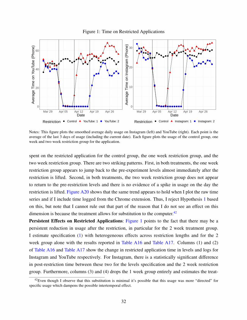
Figure 1: Time on Restricted Applications

0

20

40

60

Mar 29 Apr 05 Apr 12 Apr 19 Apr 26Date

Ave

rage

Tim

e on

You

Tube

(P

hone

)

Restriction Control YouTube: 1 YouTube: 2

0

10

20

30

Mar 29 Apr 05 Apr 12 Apr 19 Apr 26Date

Ave

rage

Tim

e on

Inst

agra

m (

Pho

ne)

Restriction Control Instagram: 1 Instagram: 2

Notes: This figure plots the smoothed average daily usage on Instagram (left) and YouTube (right). Each point is theaverage of the last 3 days of usage (including the current date). Each figure plots the usage of the control group, oneweek and two week restriction group for the application.

spent on the restricted application for the control group, the one week restriction group, and thetwo week restriction group. There are two striking patterns. First, in both treatments, the one weekrestriction group appears to jump back to the pre-experiment levels almost immediately after therestriction is lifted. Second, in both treatments, the two week restriction group does not appearto return to the pre-restriction levels and there is no evidence of a spike in usage on the day therestriction is lifted. Figure A20 shows that the same trend appears to hold when I plot the raw timeseries and if I include time logged from the Chrome extension. Thus, I reject Hypothesis 1 basedon this, but note that I cannot rule out that part of the reason that I do not see an effect on thisdimension is because the treatment allows for substitution to the computer.42

Persistent Effects on Restricted Applications: Figure 1 points to the fact that there may be apersistent reduction in usage after the restriction, in particular for the 2 week treatment group.I estimate specification (1) with heterogeneous effects across restriction lengths and for the 2week group alone with the results reported in Table A16 and Table A17. Columns (1) and (2)of Table A16 and Table A17 show the change in restricted application time in levels and logs forInstagram and YouTube respectively. For Instagram, there is a statistically significant differencein post-restriction time between these two for the levels specification and the 2 week restrictiongroup. Furthermore, columns (3) and (4) drops the 1 week group entirely and estimates the treat-

42Even though I observe that this substitution is minimal it’s possible that this usage was more “directed” forspecific usage which dampens the possible intertemporal effect.

32

ment effect for only the 2 week group. This further confirms that there is a drop of approximately5 minutes of time on Instagram on average for the Instagram restriction group. For YouTube,there is a negative, but imprecise point, estimate for both specifications. Given the skewed usagedistribution and the discrepancy between logs and levels, one might expect that the changes inpost-restriction usage are driven by those at the high end of the usage distribution. Figure A21estimates the QTE of post-restriction effects and confirms this intuition.

A natural question is, if such post-restriction effects exist, how persistent are they? It is plausi-ble that these effects dissipate very quickly, but I only observe participants for 2-3 weeks followingthe restriction. In order to understand how much longer the effects last, I rely on an optional surveythat was sent one month following the conclusion of the study asking how they had been spendingtheir time relative to before the experiment.43 Participants could mark whether they were spendinga lot less time (1), somewhat less time (2), the same amount of time (3), somewhat more time (4),or a lot more time (5). They could also mark if they did not use the application or had started to useit during the study period. I estimate the impact of the restrictions on overall phone, overall socialmedia, Instagram, and YouTube usage. Table A19 displays the estimated average treatment effect,which shows that there is still a large drop in the Instagram treatment group’s overall social mediaand Instagram usage. This result must be caveated for the following two reasons. First, there ispotential for selection bias since participants with stronger responses to the treatment may be morewilling to respond. However, roughly an equal number of participants from both the treatment andcontrol group responded, indicating this may not be a large concern.44 Second, these are unverifi-able survey responses, so it is possible that some of the results are driven by experimenter demand.Subject to these caveats, these results show that a one or two week restriction led to a reduction inusage nearly two months later. Combined with the other results, this provides evidence that therewere persistent effects of the restrictions and thus support for Hypothesis 2.Persistent Effects on Non-Restricted Applications: Table A20 and Table A21 provide estimatesfor persistent changes on usage of non-restricted applications as a result of the Instagram andYouTube treatments. I focus on applications / categories where I observed substitution towardsduring the restriction period and the applications installed during the restriction period.45 I findlittle evidence of persistent changes in usage along these dimensions. The only notable persistentincrease is in the amount of time spent on applications that were installed during the restrictionperiod for YouTube. There is a marginally significant increase in time spent on Instagram for par-

43Participants were incentivized by being able to enter the chance to win a $100 Amazon Gift Card by completingthe survey. However, they had already been paid their experimental payment after the conclusion of the study period.

44Note that since there is only partial response I do not include the controls for randomization block.45In order to economize on space I do not include in the interaction term in the reported estimates. Instead, I

estimate the ATE of the persistent for both restriction lengths (without an interaction) and then report point estimatesfor the 14-day treatment group alone.

33

ticipants in the YouTube treatment.46 However, beyond this, there are minimal persistent changeson other applications. It must be noted that these are average treatment effects and I observed het-erogeneous substitution during the restriction period itself, so it does not rule out that there werepersistent changes in time usage but that these are so heterogeneous that they would not be pickedup by this specification. Indeed, Table A18 indicates that participants self-report having persistenteffects on other applications, but the effect sizes may be too small for them to be detectable giventhe power of the experiment. However, given this evidence, I reject Hypothesis 3.

6 Model of Time Usage with Inertia

Motivated by the experimental results, I estimate an individual level discrete choice model of timeusage with inertia. There are two experimental results in particular that point to the importanceof inertia. First, participants spent time on newly installed applications and persisted to use theseapplications, even once the restriction period was over. Second, there is a reduction in usage of therestricted application in the post-restriction period, especially for the heaviest participants. Oneinterpretation of this result is that the restriction serves as a shock to participants’ habits, whichinduces them to reduce their usage of the application. In the remainder of the section, I will detailand provide estimates of the model. The main outputs of interest from the model are to quantify therole of inertia in usage and produce diversion ratios between the considered applications. Thesewill provide a more refined view of substitution between the applications of interest.

6.1 Model and Identification

I model participant’s choices as a panel of discrete choices. This is a formalization of the informalmodel in Section 5.2.1 where the participant chooses a single application at each time period touse and this choice is partially determined by the habits of the participant.47,48 There is a set ofapplications J = {1, ...J}, indexed by j, and a set of participants I = {1, ..., I}, indexed by i.I consider each application restriction as its own separate “market”, indexed by k, which dictates

46A similar effect was observed during the pilot study.47Other models of time demand for applications such as Han, Park and Oh (2015) and Yuan (2020) consider a

multiple discrete-continuous framework. Byzalov (2008) takes a similar approach as mine when considering timeallocation demand for channels on cable television. One benefit to the discrete choice approach is that it enables meto flexibly control for variation in usage throughout the day and week, which is apparent in Figure A12, as well asdirectly incorporate past usage into the utility function.

48Recall that in the experimental section there was little evidence of intertemporal substitution, evidenced by thelack of a spike of usage on the day the restriction was returned. Thus, the formulation assumes that participants aremyopic in their choices so that their usage does not directly take into account how their choice this period will impactfuture period usage.

34

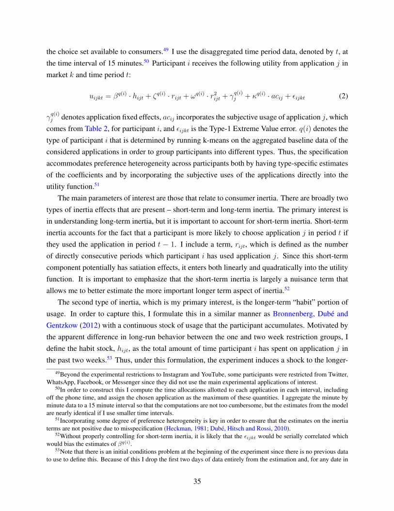
the choice set available to consumers.49 I use the disaggregated time period data, denoted by t, atthe time interval of 15 minutes.50 Participant i receives the following utility from application j inmarket k and time period t:

uijkt = βq(i) · hijt + ζq(i) · rijt + ωq(i) · r2ijt + γq(i)j + κq(i) · acij + εijkt (2)

γq(i)j denotes application fixed effects, acij incorporates the subjective usage of application j, which

comes from Table 2, for participant i, and εijkt is the Type-1 Extreme Value error. q(i) denotes thetype of participant i that is determined by running k-means on the aggregated baseline data of theconsidered applications in order to group participants into different types. Thus, the specificationaccommodates preference heterogeneity across participants both by having type-specific estimatesof the coefficients and by incorporating the subjective uses of the applications directly into theutility function.51

The main parameters of interest are those that relate to consumer inertia. There are broadly twotypes of inertia effects that are present – short-term and long-term inertia. The primary interest isin understanding long-term inertia, but it is important to account for short-term inertia. Short-terminertia accounts for the fact that a participant is more likely to choose application j in period t ifthey used the application in period t − 1. I include a term, rijt, which is defined as the numberof directly consecutive periods which participant i has used application j. Since this short-termcomponent potentially has satiation effects, it enters both linearly and quadratically into the utilityfunction. It is important to emphasize that the short-term inertia is largely a nuisance term thatallows me to better estimate the more important longer term aspect of inertia.52

The second type of inertia, which is my primary interest, is the longer-term “habit” portion ofusage. In order to capture this, I formulate this in a similar manner as Bronnenberg, Dube andGentzkow (2012) with a continuous stock of usage that the participant accumulates. Motivated bythe apparent difference in long-run behavior between the one and two week restriction groups, Idefine the habit stock, hijt, as the total amount of time participant i has spent on application j inthe past two weeks.53 Thus, under this formulation, the experiment induces a shock to the longer-

49Beyond the experimental restrictions to Instagram and YouTube, some participants were restricted from Twitter,WhatsApp, Facebook, or Messenger since they did not use the main experimental applications of interest.

50In order to construct this I compute the time allocations allotted to each application in each interval, includingoff the phone time, and assign the chosen application as the maximum of these quantities. I aggregate the minute byminute data to a 15 minute interval so that the computations are not too cumbersome, but the estimates from the modelare nearly identical if I use smaller time intervals.

51Incorporating some degree of preference heterogeneity is key in order to ensure that the estimates on the inertiaterms are not positive due to misspecification (Heckman, 1981; Dube, Hitsch and Rossi, 2010).

52Without properly controlling for short-term inertia, it is likely that the εijkt would be serially correlated whichwould bias the estimates of βq(i).

53Note that there is an initial conditions problem at the beginning of the experiment since there is no previous datato use to define this. Because of this I drop the first two days of data entirely from the estimation and, for any date in

35

term habit portion of usage, but, beyond the initial period when the restrictions are lifted, not theshort-run inertia portion.

The granularity of the data allows me to vary the outside option flexibly across time. For anytime index t, I allow the outside option to vary across the week of the experiment w(t), day of theweek d(t), and hour of the day o(t). I collapse the hours of the day into morning (7 AM - 12 PM),afternoon (12 PM - 6 PM), evening (6 PM - 1 AM), and late night (1 AM - 7 AM). I normalizethe outside option to zero at afternoons, Fridays, and the final week of the experiment. Thus, theutility for the outside option is denoted as follows where αo(t) denotes hour of day fixed effects,ιd(t) denotes day of week fixed effects, and µw(t) denotes week fixed effects:

ui0tk = αo(t) + ιd(t) + µw(t) + εi0tk

The assumption that εijkt are independent and identically distributed according to a Type-1 extremevalue distribution induces the following probability that application j will be chosen by participanti:

l(hijt, aij , rijt; θ) =exp(βq(i) · hijt + ζq(i) · rijt + ωq(i) · r2ijt + γ

q(i)j + κq(i) · acij)

exp(αo(t) + ιd(t) + µw(t)) +∑

j′ exp(βq(i) · hij′t + ζq(i) · rij′t + ωq(i) · r2

ij′t + γq(i)j′ + κq(i) · acij′ )

(3)

Identification: The primary parameter of interest is βq(i). The identification argument for thisparameter is as follows. First, following the literature on state-dependent demand estimation (e.g.Dube, Hitsch and Rossi (2010)), it is important that the specification sufficiently captures individ-ual preference heterogeneity. This is captured by incorporating the subjective usage of each ofthe considered applications as well as having type-specific estimates.54 Second, the experimentinduces exogenous variation in the habit stock of the restricted applications as well as the other ap-plications (via substitution during the restriction period). Thus, the core identification assumptionis that the experiment only serves as a shock to the habits of the participants.Estimation: I restrict myself to the most prominent social media and entertainment applications– Facebook, TikTok, Twitter, Reddit, YouTube, Instagram, and Snapchat – and denote every otherapplication or off phone activity as the outside option. For these applications, I collect the average

the first two weeks, I multiply the accumulated “stock” by the inverse of the fraction of the current time period by thetime period exactly 2 weeks from the start of the experiment. I chose two days since the descriptive statistics point tousage not varying drastically across the days of the week and preliminary experiments showed that after two days thehabit stock variable is fairly constant in the baseline period.

54The biggest worry about unobserved heterogeneity in usage comes from the extreme users of specific applicationsor bundles of applications. The clustering formulation is able to capture the differences in preference intensity forthese participants and consider separate estimates for them. The approach of discretizing a potentially continuousdistribution of unobserved heterogeneity through k-means has precedent in Bonhomme, Lamadon and Manresa (2017).

36

daily usage in the baseline period for each participant and cluster the participants according tok-means. I then estimate the model separately for each type. Since my model is likelihood-based,I estimate the parameters using maximum likelihood estimation.

6.2 Model Estimates and Validation

The first step of estimation requires classifying the participants into different types using k-means.There is a large literature in data mining and statistics about choosing the “optimal” k that trades offthe parsimony of having fewer clusters against the reduction in within-cluster variance that arisesfrom additional clusters. In this case an additional consideration is that it is important to ensure thatthe clusters have sufficiently many individuals to allow for estimation of the parameters of interestfor this group, but also having sufficiently many clusters to capture the unobserved preferenceheterogeneity. I consider an index of these measures for choosing the “optimal” k which reportsk = 3 and k = 6. In order to accommodate additional heterogeneity in consumer preferences,I utilize k = 6.55 Figure A22 displays the resulting clusters and the time allocations within eachof them. The resulting clustering of participants identifies sets of power users. Cluster 1 capturesthe more typical users of these applications who have moderate usage of each of the applications.Clusters 2 and 3 capture the YouTube intensive participants. Cluster 4 captures the power usersof Reddit. Cluster 5 identifies participants who are power users of TikTok, but also use the othersocial media applications extensively. Cluster 6 identifies participants who are power users ofFacebook and Instagram.

The estimates from the model are presented in Table A24. I report the estimates of each typeseparately. The first observation is that the coefficient on hijt is fairly consistent across the differ-ent types as well as the estimate for the influence of short-term inertia, rijt and r2ijt. Both of theseterms are statistically different from 0, indicating that both the short-term and long-term inertiachannels play a role. The coefficient on r2ijt is negative, indicating satiation effects. The differ-ences in the natural usage of each of the applications across the different types, which is reflectedin Figure A22, naturally translates to differences in the estimated application fixed effects. Theestimated time fixed effects that vary the outside option are similar across the different types andfollow the variation in phone usage across the week depicted in Figure A12. The coefficients onthe different subjective uses of the applications varies across the types in accordance with the mostused applications by participants classified as that type.

55I additionally consider density-based spatial clustering of applications with noise (DBSCAN) (Ester et al., 1996)and spectral clustering (Von Luxburg, 2007) which are clustering algorithms that do not restrict themselves to convexregions. Following best practices for the methods, I find that they do not result in substantially different clusteringswith DBSCAN leading to 3 clusters and spectral clustering leading to 7. Both pick out similar clusterings as k-meanswith k = 3 and k = 6, so I opt for using k-means.

37

I validate the in-sample fit of the model by comparing how well the model is able to match theactual market shares throughout the study period. Recall that the model is estimated including therestriction period. Thus, I compare how well the model is able to predict the average market sharesin the non-restriction period in addition to how well it is able to predict the substitution duringthe restriction period. In particular, I compare how well the model is able to capture substitutiontowards other applications and the outside option in the Instagram and YouTube restriction periodsrespectively. Table A25 shows that the model fits the data reasonably well as it matches the non-restriction period market shares and predicts the extent of substitution towards other applicationsand the outside option as a result of the experimental restrictions.56

Table 7: Second-Choice Diversion Ratios

Instagram Twitter YouTube TikTok Reddit Snapchat Facebook Outside Option

Instagram - 0.0047 0.023 0.0063 0.0029 0.0072 0.013 0.94Twitter 0.027 - 0.025 0.013 0.0041 0.0059 0.012 0.91

YouTube 0.024 0.0044 - 0.0071 0.0081 0.0055 0.011 0.94TikTok 0.028 0.0092 0.03 - 0.0029 0.019 0.012 0.9Reddit 0.014 0.003 0.034 0.0034 - 0.0052 0.0079 0.93

Snapchat 0.026 0.0036 0.022 0.018 0.0047 - 0.011 0.91Facebook 0.026 0.0042 0.023 0.0061 0.0037 0.0064 - 0.93

Notes: This table displays the estimated second-choice diversion ratios that come from the estimated model. The cell in each rowk and column j is computed by Dkj =

sj(J\{k})−sj(J )sk(J ) .

The primary output of the estimated model is the second-choice diversion ratio. The second-choice diversion ratio between application j and k provides an estimate of what fraction of con-sumption of application k would shift from application k to application j when application k wasremoved from the choice set. Typically, regulatory authorities use second-choice diversion ratioscoming from switching surveys as a critical input to merger evaluation (Reynolds and Walters,2008; Conlon and Mortimer, 2018) and this input will be crucial for the merger exercise conductedlater in the paper. In order for the model to provide reasonable estimates for this quantity it isimportant that it is able to predict how participants would substitute towards the other applica-tions if the application was not available. The model validation exercises showed that the modelis able to do this for the Instagram and YouTube restrictions and thus ought to provide a reason-able estimate of this quantity. Table 7 displays the estimated diversion ratios, which are given by

56The estimates of the main parameters of interest are robust to model specification. Preliminary specificationsdid not include application fixed effects, but rather only included application characteristics and were estimated overthe entire sample. Over these different specifications, the model had a poorer fit of the overall data, but had a similarestimate of roughly 0.01 for hijt across the different types. Furthermore, omitting either the short-term inertia orsubjective application usage from the utility function leads to an increase in the coefficient of hijt but does not changethe resulting estimates or main outputs from the model dramatically.

38

Djk =sj(J\{k})−sj(J )

sk(J ). Each of the predicted shares is computed as before, by a weighted average

over the different types according to the fraction of participants assigned to a type. The diversionratios across each of the different applications predict a large amount of diversion to the outsideoption, with Instagram and YouTube having the highest diversion towards the outside option.

An alternative approach to compute the second-choice diversion ratios is to directly utilize theestimated average treatment effects of substitution during the product unavailability period. Conlonand Mortimer (2018) provide a treatment effects interpretation of second-choice diversion ratiosthat does this and, in Conlon, Mortimer and Sarkis (2021), provide a method to compute the restof the matrix of diversion ratios for applications without experimental variation. In Appendix E,I apply their methods to get an alternative estimate of the diversion ratios, shown in Table A22.The estimated diversion ratios are similar to those estimated using the model. The main noticeabledifference is that the diversion between, for instance, Instagram-Facebook, YouTube-Instagram,and Instagram-TikTok is noticeably larger than the estimates produced from the model. This isdue to the fact that these are nonparametric and driven by the difference in point estimates of thetreatment effects. The nonparametric diversion ratio estimates are displayed in Table A23, whichshows the degree of imprecision in their estimation. This is since the power requirements to getprecisely estimated diversion ratios are not just being able to distinguish the estimated substitutiontowards one application as being greater than zero, but rather being able to distinguish estimatedsubstitution towards one application as being greater than other applications with positive substi-tution. Thus, my experiment is not sufficiently powered to determine whether these differences inthe estimated diversion ratios come from imprecision or actual differences. As a result, I rely onthe estimated diversion ratios from the model.57

6.3 Counterfactual: No Inertia

The counterfactual I consider is to understand the role of the long-term inertia channel in drivingthe usage of the social media and entertainment applications. Concretely, I impose βq(i) = 0 andcharacterize the change in the resulting market shares and diversion ratios, which will allow me toconsider how this channel influences merger assessments in Section 7. It is important to understandthe interpretation of this counterfactual since it is not a direct policy counterfactual. This inertiachannel comprises a number of different aspects of usage – ranging from addictive impulses tomore natural mechanisms behind inertia such as switching costs. There are several interpretationsof the counterfactual that are directly motivated by regulatory and antitrust concerns.

First, the diversion ratios produced under the no inertia counterfactual are more natural mea-sures of substitution between the applications than in the baseline. This is since the baseline di-

57Another important consideration is that this method does not allow me to consider how the diversion ratio changeswith and without inertia.

39

version ratios include the extent of diversion due to both direct substitutability and habitual usage.This leads to naturally higher diversion for applications with higher habitual usage (e.g. Instagram,YouTube). Thus, the diversion ratios produced by the no inertia counterfactual are plausibly morepolicy-invariant measures of diversion that focus only on the direct substitutability of any giventwo applications.

Second, while some aspects of inertia are natural components of decision-making, there areaddictive elements of these applications and a number of policy instruments have been proposedfor alleviating this issue. For instance, the contention that the curation algorithms optimize onlyfor user engagement and that design patterns such as infinite scroll news feeds encourage exces-sive usage of these applications has fueled a debate about whether regulations should be imposedon these algorithms and design patterns (Narayanan et al., 2020). There are additionally policyproposals aimed at directly limiting the time spent on these applications. Thus, one interpretationof the counterfactual is to understand the limit case of effectiveness of these proposed regulationsand what impact they would have from an antitrust perspective. It is due to this that I only considershutting down the long-term inertia channel and not the short-term channel.

Third, it is common in this market for the larger firms such as Facebook or Google to acquire asmaller firm before it gains critical mass and thus the counterfactual captures the limit case whenthe larger firm acquires the smaller firm before the smaller firm is able to build up the habit stock ofconsumers. In this case, the more interesting comparison is in the opposite direction; the measuresof diversion observed at the time of the merger might not capture the extent of diversion once theapplication is acquired and continues to builds up the habit stock of consumers.58

Table 8 compares the average market shares with and without the inertia term across differentweeks of the experiment when participants had the full set of applications available to them. Sincethe results across the different subsets of weeks are quantitatively very similar, I restrict focusto the first two columns which compare the differences across all weeks in the experiment. Thefirst observation is that the overall market share of the set of inside applications drops by nearly40% when this channel is shut down.59 Table A28 displays the reduction of usage in percentages,showing that YouTube, Instagram, and TikTok have the largest percentage reduction in averageusage when this channel is shut down. Recall that TikTok in particular has a smaller number of

58This was one purported motivation for instance behind the Facebook and Instagram merger, seehttps://www.theverge.com/2020/7/29/21345723/facebook-instagram-documents-emails-mark-zuckerberg-kevin-systrom-hearing.

59This observed decrease is qualitatively similar across other model specifications. Allowing application-specificcoefficients on hijt leads to a quantitatively identical change in the overall usage of the applications. A separate modelmodel specification that did not include application fixed effects and instead used application characteristics reporteda range of 32-40% reduction in overall usage. Furthermore, concurrent work by Allcott, Gentzkow and Song (2021)estimates a similar quantity using a substantially different model specification, a slightly different set of applications,and experimental design and find a 31% reduction.

40

users in my sample relative to the other applications, but, conditional on using the application, hasone of the highest average time allocations. As a result, it is not too unsurprising that the modelpredicts that inertia is a large driver of usage for this application. I further compute the estimatedsecond-choice diversion ratios when the inertia channel is shut down. The estimates are displayedin Table A26 with the percentage differences between the baseline and no inertia case presentedin Table A27. The reduction in the diversion ratios is roughly consistent with the drop in marketshare for the application.

Table 8: Market Shares (No Inertia)

ApplicationNo Inertia:

Weeks 1,4,5Baseline:

Weeks 1,4,5No Inertia:Weeks 4,5

Baseline:Weeks 4,5

No Inertia:Week 1

Baseline:Week 1

Instagram 0.0148 0.0276 0.0149 0.0276 0.0145 0.0275Outside Option 0.941 0.901 0.94 0.899 0.943 0.904

Twitter 0.00364 0.0044 0.00371 0.0045 0.00345 0.00411YouTube 0.0191 0.0339 0.0195 0.0347 0.0179 0.0318TikTok 0.00388 0.00797 0.00392 0.00817 0.00376 0.00743Reddit 0.00471 0.00644 0.00479 0.00673 0.00447 0.00563

Snapchat 0.00456 0.00679 0.00456 0.00682 0.00456 0.00672Facebook 0.00852 0.0122 0.00858 0.0121 0.00833 0.0124

Notes: Columns 1 and 2 display the predictions of the model over week 1, 4, and 5 including the long-term inertia termand without. Columns 3 and 4 display the prediction of the model only over weeks 4 and 5. Columns 5 and 6 displaythe prediction of the model only over week 1. Each cell displays the market share of the row application under thespecification designated by the column.

7 Merger Analysis

In this section I conduct hypothetical merger analysis between the prominent social media andentertainment applications. I propose a variant of the standard Upward Pricing Pressure (UPP)test for attention markets and then use the estimated diversion ratios from Section 6 to implementthis test. I implement the test using the estimated diversion ratios with and without inertia andcharacterize which merger decisions would change due to the influence of inertia.

7.1 Upward Pricing Pressure Test

In order to evaluate a merger between two applications, I need to specify the profit function of theapplications and, importantly, their choice variables. I retain the same notion discussed in Sec-

41

tion 5.1.3 where the primary choice variable of the applications is to set the attention costs facedby consumers. I follow the literature on two-sided media markets by supposing that the primarymanifestation of this is through choosing the advertising load of the application – the number ofadvertisements per unit time experienced by the consumer. The model is necessarily stylized, butcaptures the fundamental elements of the market.

Formally, I consider that the applications are playing a Bertrand-Nash game where each ap-plication j sets its advertising load in order to maximize profits. The application revenue per unittime depends on the quantity of advertisements per unit time, aj , and the price that advertisers arewilling to pay for advertising on this application, Pj(tj(a)), which depends on the time allocationsof consumers, tj(a). The marginal cost of the application, denoted cj , is the marginal cost of serv-ing these advertisements to consumers. Thus, the profit maximization problem for application j isgiven by:

argmaxaj

πj(a) = (aj · Pj(tj(a))− cj) · tj(a) (4)

Consumers face differentiated goods where the main “price” that they face is the advertising quan-tity set by the application, which induces a disutility that depresses their time allocations. Adver-tising is modeled as a homogenous good that is differentiated only through the time that consumersspend on the application. This is the main channel through which network effects show up in thisformulation as it captures that advertisers have a willingness to pay that varies with the ability totarget consumers and depends on the time allocations of consumers. The prices are set throughsecond-price auctions so that they reflect the willingness to pay of advertisers to acquire the atten-tion of the consumers on that application at a given point in time. Consequently, the applicationdoes not directly set the advertising prices.

Given this formulation, I propose an Upward Pricing Pressure (UPP) test to conduct mergeranalysis (Farrell and Shapiro, 2010). The goal of the test is to determine whether a merger wouldlead to “upward pressure” on prices and, if so, the merger is blocked. The effect of a merger isambiguous since it exerts upward pressure on prices by enabling the firm to internalize the diver-sion between the merged firms’ applications, but also puts downward pressure on prices throughthe efficiency gains resulting from the merger. In this setup, the relevant quantity is not whetherthe merger induces higher prices, but whether it induces higher advertising loads.

In order to formulate the test, I need to specify the joint profit function of the merged firm. Themain change is that the merger induces efficiency gains that arise through an increase in the qualityof the applications. Following Willig (2011), I incorporate this by supposing that consumers face aquality-adjusted advertising load. One possible interpretation of this is that the increased ability totarget advertising leads to more useful advertisements for consumers, though the quality gains arebroader than just the impact on advertising. Thus, the merged profit function between applications

42

1 and 2 is as follows:

π1 + π2 =(P1(t1(a)) · (a1 + ν1)− c1

)· t1(a) +

(P2(t2(a)) · (a2 + ν2)− c2

)· t2(a)

where ν1, ν2 denote the quality gains for application 1 and 2 respectively as a result of the merger.The UPP evaluates whether, for each application individually, the first-order condition of themerged profit function is positive (i.e. whether ∂(π1+π2)

∂a1> 0 or ∂(π1+π2)

∂a2> 0) when evaluated

at the current equilibrium advertising loads and prices (e.g. the pre-merger advertising loads andprices). The derivation of the UPP test is provided in Appendix G and is given by:

UPP1 = D12 ·(P2 · (a2 + ν2)− c2︸ ︷︷ ︸

Revenue from Diversion

+dP2

dt2· (a2 + ν2) · t2(a)︸ ︷︷ ︸

Price Change from Diversion

)−(ν1 ·

(dP1

dt1· t1(a) + P1

)︸ ︷︷ ︸

Quality Efficiency Gains

)

D12 denotes the diversion ratio from application 1 to 2. There are two separate channels thatput upwards pressure on the quality-adjusted advertising load faced by consumers. The first is thatthe diversion towards application 2 from application 1’s increase in advertising load enables theapplication to gain additional revenues due to the additional time spent on the application. Thesecond captures the impact of the diversion towards application 2 on the advertising prices forapplication 2. There is one channel that puts downward pressure on the quality-adjusted advertis-ing load, which is that the merger induces quality improvements. This quality gain could comethrough a number of channels, such as improved curation algorithms, better product infrastructure,or improvements in advertising targeting.

7.2 Data and Additional Discussion

In order to be able to conduct merger evaluation using the UPP test, I need to collect or estimatethe following quantities. I require data on the advertising quantities, advertising prices, time allo-cations of consumers, and marginal costs. Further, the test necessitates an estimate of consumerdiversion between the two applications being merged as well as an estimate for how responsiveadvertising prices are to additional time spent on an application.Advertising Load and Prices Data: The data that I use is as follows. The time allocation datacomes from the baseline period during the experiment. The advertising load data comes fromself-reported data from experimental participants where they were asked to report how many ad-vertisements they experience per minute of usage on each of the applications. I take the averageacross all the participants to get a measure of the advertising load for each application. The ad-vertising price data comes from the average price per impression on each application in 2021 as

43

reported in trade blogs.60 Finally, I suppose that the marginal cost of serving advertisements iszero.61

Measure of Consumer Diversion: The main variable in the UPP formulation that comes fromconsumer demand is the estimated diversion ratio. In the UPP formulation, it enters as − ∂t2

∂a1/ ∂t1∂a1

,which is the diversion ratio with respect to advertising load. Since the advertising load is constantover the period of the study, I do not have the variation to identify the advertising load coefficient,and consequently the diversion ratio with respect to advertising load, in a demand model. However,the product unavailability variation and estimated model in Section 6 provides me with an estimateof the second-choice diversion ratio. Second-choice diversion ratios are commonly used insteadof price-based diversion ratios in merger evaluation cases (Reynolds and Walters, 2008; Conlonand Mortimer, 2018). Furthermore, Conlon and Mortimer (2018) show that the difference betweenthese estimates depends on the curvature of demand with respect to the variable of interest. Thismeans that whether or not second-choice diversion ratios are reasonable proxies for advertisingload diversion ratios depends on the curvature of demand with respect to advertising load. Themain empirical evidence from the literature on the relationship between advertising loads and timeallocations comes from Huang, Reiley and Riabov (2018) who show a strikingly linear relationshipbetween time allocations and advertising load in a 21 month experiment on Pandora. Followingthe results of Conlon and Mortimer (2018), this linearity indicates that second-choice diversionratios should provide a reasonable approximation to diversion with respect to advertising load.Advertising Price Setting: The modeling of the advertising market requires some additional dis-cussion as it is stylized on several dimensions. The assumption that advertising, holding constantconsumer time allocations, is a homogeneous good is consistent with qualitative evidence in CMA(2020) and discussions with industry professionals who state that the primary determining factorof where to spend their advertising budget is the reach and ability to target on the application.62,63

The assumption that the applications do not explicitly set prices is consistent with practice whereadvertising prices are typically set via generalized second-price auctions.

The formulation utilizes the following assumptions on how components of the model impact

60Note that these prices are relatively low. For instance the average price per impression on Instagram is $0.00791,which is contrast to the larger value of additional time on the application documented in Appendix C.

61This is a reasonable approximation since the marginal cost of serving an individual advertisement involves thecomputational cost of coordinating a (generalized) second-price auction and serving an HTTP request. This is com-mon in technology infrastructure where fixed costs are relatively high, but the marginal cost of network requests isnegligible.

62The main differentiation factor beyond this that is within control of the application is the advertising form – forinstance the distinction between video and non-video advertising is considered important. However, this is generallyconsidered secondary to the targeting aspect and thus I omit it from modeling considerations.

63In this formulation I am only focusing on the price of an impression. In reality advertisers pay a price based onthe number of impressions (denoted CPM) and the number of clicks (denoted CPC). If I make the assumption thatthe click-through rate is identical across applications then this can alternatively interpreted as CPC instead of CPM.However, I do not explicitly model these two channels separately.

44

advertising prices. The first assumption is that advertising is a homogenous good whose maindifferentiation is through the reach and targeting that depends on consumer time spent on theapplication. The second is that the price does not change based on the advertising load.64 Thusthe only channel through which an application is disincentivized from increasing its advertisingload is through the disutility incurred by consumers and the resulting impact on advertising price.For the UPP exercise, I only consider that the elasticity of advertising price with respect to timeis non-negative. This is since the advertisements in the applications of interest are predominantlybehaviorally targeted display advertising, which crucially is reliant on consumer histories in orderto target advertising effectively. The literature in marketing that quantifies the value of consumer-specific information on the willingness to pay of advertisers in these markets finds a substantialincrease in advertiser willingness to pay as a result of having this information (Beales and Eisenach,2014; Aziz and Telang, 2016; Johnson, Shriver and Du, 2020).65 Thus, due to these assumptions,I naturally consider evaluating mergers on a grid of parameters where dP1

dt1= dP2

dt2.

Quality Efficiency Gains: I suppose that the merger induces efficiency gains through improvedapplication quality. Predicting the extent of these efficiency gains at the time of a merger is achallenging problem and the typical approach is to assign a fixed efficiency credit as a result of themerger (Farrell and Shapiro, 2010). The efficiency credit assignment is typically done by settingthe value of this parameter to a fraction of the pre-merger quantity. In this case, when consideringwhether there is upward pressure for application i when evaluating a merger between applicationsi and j, I set νi = 0.1 · a∗i and νj = 0 so that the efficiency credits for application i are set to be10% of the pre-merger advertising levels.

7.3 Merger Evaluation

All of the terms in the UPP formulation are specified besides dP1

dt1. In order to provide sharper

intuition about the different mechanisms at play, I consider two separate cases to provide a cleanercharacterization of the results: zero advertising price elasticity, dP1

dt1= 0, and non-zero advertising

price elasticity, dP1

dt1> 0. I consider these cases using the diversion ratios with inertia and then

without inertia with the results summarized in Table 9.

64These two aspects implicitly rely on the following two assumptions. The first is that there are no explicit crowdingout effects between advertisers when the quantity of advertisements on a single application is increased. The second isthat I have omitted directly specifying advertiser payoffs, but one possible (strong) assumption would be if advertisersare homogeneous in the value of a conversion. In this case the price increase from additional time allocations is thatadditional precision in targeting increases the probability of conversion, thus increasing the price they are willing topay for the unit of attention.

65An additional piece of evidence for this is in Aridor, Che and Salz (2020) who study the value of consumers toadvertisers after the EU’s General Data Protection Regulation and argue that more persistently trackable consumersresult in an increase in the valuation of an average consumer.

45

Table 9: Summary of UPP Merger Analysis

dP1

dt1= 0 dP1

dt1> 0

With InertiaSnapchat-Instagram, Reddit-Instagram,Snapchat-YouTube, Reddit-YouTube,

Reddit-Facebook

Snapchat-Instagram, Reddit-Instagram,Snapchat-YouTube, Reddit-YouTube,Twitter-YouTube, TikTok-Instagram,TikTok-YouTube, Twitter-Instagram

Without InertiaReddit-YouTube, Reddit-Instagram,

Snapchat-YouTubeReddit-YouTube, Reddit-Instagram,

Snapchat-YouTube

Notes: This table summarizes the results of the UPP merger analysis exercise. I consider mergers between each pair ofapplications in the list: YouTube, Instagram, Snapchat, Reddit, Instagram, TikTok, Twitter, Facebook. I do not considerthe fact that Facebook and Instagram are jointly owned and, consequently, do not consider a hypothetical merger betweenthe two. For the case when dP1

dt1> 0, I report the results when dP1

dt1> 0.004.

7.3.1 Merger Evaluation With Inertia

For each case, I compute the UPP for the merger between each pair of applications and reportwhich gets blocked. Recall that a merger is blocked if UPPi > 0 is larger than zero for at leastone of the applications i involved in the merger.66

Zero Advertising Price Elasticity: This assumption isolates the tradeoff between the (Revenue

from Diversion) and (Quality Efficiency Gains) terms. In this case, the following mergers getblocked: Snapchat-Instagram, Reddit-Instagram, Snapchat-YouTube, Reddit-YouTube, Reddit-Facebook. These are predominantly mergers between smaller applications with relatively lowadvertising loads and prices (i.e. Reddit, Snapchat) and larger applications (i.e. Facebook, Insta-gram, YouTube). This is primarily caused by upward pressure on advertising load for the smallerapplication. There are two underlying reasons behind this. First, there is relatively high upwardpressure due to diversion from the smaller to the larger applications. By increasing advertisingload and inducing time substitution towards the larger applications, the joint firm earns additionalrevenues since a large share of time gets diverted towards the larger application and a single unit oftime on e.g. Instagram is more valuable than a single unit of time on e.g. Reddit. Second, there isrelatively lower downward pressure since these smaller applications have lower advertising loadsinducing smaller values for the efficiency gain threshold.Non-Zero Advertising Price Elasticity: Now I consider the case when the own advertising priceelasticity is non-zero. This introduces additional upward pressure relative to the previous casesince now the (Price Change from Diversion) term is non-zero, which depends on the own-price

66Note that I do not include Facebook-Instagram since these applications are already merged in reality and, formergers involving these applications, I do not explicitly take into account the joint effect of these.

46

elasticity with respect to time as well as the pre-merger advertising load and average time allo-cations of application 2. However, it also induces additional downward pressure that depends onthe own-price elasticity with respect to time and the pre-merger average time allocations of ap-plication 1. I consider the grid of dP1

dt1= dP2

dt2∈ {0.0001, 0.0002, ..., 0.009}, which leads to the

same set of mergers to be blocked as in the zero advertising price elasticity case, with the oneexception of Reddit-Facebook. Once dP1

dt1> 0.0004, then the following mergers also get blocked:

Twitter-YouTube, TikTok-Instagram, TikTok-YouTube, Twitter-Instagram. In this case, the samemechanism as before is at play – there is an incentive for the merged firm to increase advertisingloads from the smaller application (e.g. TikTok) to divert additional time towards the larger appli-cations. Since the average time allocations on the larger application are higher than on the smallerapplication, the upward pressure wins out relative to the downward pressure and induces additionalupward pressure relative to the previous case. This is not always the case, however, as evidencedby the fact that the Reddit-Facebook merger is no longer blocked.

7.3.2 Merger Evaluation Without Inertia

I consider the same merger evaluation exercises under the counterfactual that the inertia channelis shut down. This leads to two changes in the UPP evaluation relative to Section 7.3.1: the timeallocations across applications are lower, given by Table 8, and the subsequent diversion betweenthe applications is lower for most of the applications, given by Table A26. Note that the percentagechanges in the diversion ratios and market shares relative to the baseline inertia case are providedin Table A27 and Table A28.Zero Advertising Price Elasticity: In this case, the only term which changes relative to the iner-tia baseline is the diversion weights on (Revenue from Diversion). This means that the downwardpressure remains the same as before, but the upward pressure is potentially softened due to thedecrease in diversion between these applications. Due to this, the following mergers are no longerblocked: Snapchat-YouTube, Reddit-Facebook. However, Reddit-YouTube, Reddit-Instagram,and Snapchat-Instagram remain blocked indicating that the softening of diversion between theseapplications due to the lack of inertia is not sufficiently strong to induce all mergers to not beblocked.Non-Zero Advertising Price Elasticity: I consider the same range for dP1

dt1as before. In this case,

both the additional upward and downward pressure are suppressed due to the lack of inertia. Theupward pressure from (Price Change from Diversion) is suppressed due to the decrease in diversionas well as the decrease in the average time allocations on application 2. The downward pressuredue to (Quality Efficiency Gains) is suppressed due to the decrease in average time allocationson application 1. In the cases when a merger was previously blocked, the upward pressure issoftened more relative to the downward pressure, which leads to the following mergers no longer

47

being blocked across all values in the set of considered parameters: TikTok-Instagram, TikTok-YouTube, Twitter-Instagram, Snapchat-YouTube, and Twitter-YouTube. Indeed, not only are noadditional mergers blocked beyond those that were present before including this channel, but, fordP1

dt1> 0.0002, even the merger between Reddit and Instagram is no longer blocked. Thus, in this

case the role of inertia is so strong that it is the primary reason for blocking the mergers betweenthese applications.

8 Conclusion

In this paper I report the results of an experiment where I continuously monitor how participantsspend time on digital services and shut off their access to Instagram or YouTube for one or twoweeks. I use the resulting data on how participants substitute their time during and after the re-strictions in order to uncover a rich picture of the demand for social media and entertainmentapplications. I illustrate how the estimated substitution patterns can be used to guide questions ofmarket definition and merger evaluation of these applications that have troubled regulators due tothe fact that consumers pay no monetary price to use these services.

I find that participants with the YouTube restriction spend time on applications installed duringthe restriction period and that participants with the two week Instagram restriction reduce theirtime spent on Instagram even after the restrictions are lifted. Motivated by this, I estimate a discretechoice model of time usage with inertia and find that inertia accounts for a substantial fraction ofusage. Finally, I develop an Upward Pricing Pressure Test for attention markets and show thatthe presence of inertia is crucial for justifying blocking several mergers between social mediaapplications.

Overall, my results emphasize the usefulness of product unavailability experiments for demandand merger analysis in attention markets. As shown in this paper, they provide a clean way of mea-suring substitution patterns in these markets as well as identifying addiction/inertia effects, whichhave been documented as first-order components of competition between these services. Theseexperiments are feasible to conduct for regulatory authorities since the nature of digital goods en-ables individual level, randomized controlled experiments of product unavailability. My resultspoint to a broad competition for time between social media applications, but also emphasizes thatinertia drives a substantial fraction of their usage and diversion towards larger applications suchas Facebook and YouTube. This latter point indicates that digital addiction issues in these marketsare not only important in their own right, but also important from an antitrust perspective. I believethat the insights from this paper can help push forward the regulatory debate about such marketsand lead to a better understanding of these zero price attention markets.

48

References

Abadie, Alberto, Joshua Angrist, and Guido Imbens. 2002. “Instrumental variables estimates ofthe effect of subsidized training on the quantiles of trainee earnings.” Econometrica, 70(1): 91–117.

Affeldt, Pauline, Lapo Filistrucchi, and Tobias J Klein. 2013. “Upward pricing pressure intwo-sided markets.” The Economic Journal, 123(572): F505–F523.

Allcott, Hunt, Luca Braghieri, Sarah Eichmeyer, and Matthew Gentzkow. 2020. “The welfareeffects of social media.” American Economic Review, 110(3): 629–76.

Allcott, Hunt, Matthew Gentzkow, and Lena Song. 2021. “Digital Addiction.” Working Paper.Ambrus, Attila, Emilio Calvano, and Markus Reisinger. 2016. “Either or both competition: A”

two-sided” theory of advertising with overlapping viewerships.” American Economic Journal:

Microeconomics, 8(3): 189–222.Andersen, Steffen, Glenn W Harrison, Morten Igel Lau, and E Elisabet Rutstrom. 2006.

“Elicitation using multiple price list formats.” Experimental Economics, 9(4): 383–405.Anderson, Simon P, and Stephen Coate. 2005. “Market provision of broadcasting: A welfare

analysis.” The Review of Economic Studies, 72(4): 947–972.Anderson, Simon P, Øystein Foros, and Hans Jarle Kind. 2018. “Competition for advertisers

and for viewers in media markets.” The Economic Journal, 128(608): 34–54.Andreassen, Cecilie Schou, Torbjørn Torsheim, Geir Scott Brunborg, and Stale Pallesen.

2012. “Development of a Facebook addiction scale.” Psychological reports, 110(2): 501–517.Aridor, Guy, Yeon-Koo Che, and Tobias Salz. 2020. “The economic consequences of data pri-

vacy regulation: Empirical evidence from gdpr.” National Bureau of Economic Research.Athey, Susan, Emilio Calvano, and Joshua S Gans. 2018. “The impact of consumer multi-

homing on advertising markets and media competition.” Management Science, 64(4): 1574–1590.

Aziz, Arslan, and Rahul Telang. 2016. “What is a Digital Cookie Worth?” Available at SSRN

2757325.Bailey, Erica R, Sandra C Matz, Wu Youyou, and Sheena S Iyengar. 2020. “Authentic self-

expression on social media is associated with greater subjective well-being.” Nature communi-

cations, 11(1): 1–9.Bakshy, Eytan, Solomon Messing, and Lada A Adamic. 2015. “Exposure to ideologically di-

verse news and opinion on Facebook.” Science, 348(6239): 1130–1132.Baym, Nancy K, Kelly B Wagman, and Christopher J Persaud. 2020. “Mind-

fully Scrolling: Rethinking Facebook after Time Deactivated.” Social Media+ Society,6(2): 2056305120919105.

49

Beales, Howard, and Jeffrey A Eisenach. 2014. “An empirical analysis of the value of informa-tion sharing in the market for online content.” Available at SSRN 2421405.

Bellemare, Marc F, and Casey J Wichman. 2019. “Elasticities and the inverse hyperbolic sinetransformation.” Oxford Bulletin of Economics and Statistics.

Berry, Steven, and Philip Haile. 2016. “Identification in differentiated products markets.” Annual

review of Economics, 8: 27–52.Bhat, Chandra R. 2008. “The multiple discrete-continuous extreme value (MDCEV) model: role

of utility function parameters, identification considerations, and model extensions.” Transporta-

tion Research Part B: Methodological, 42(3): 274–303.Bonhomme, Stephane, Thibaut Lamadon, and Elena Manresa. 2017. “Discretizing unobserved

heterogeneity.” University of Chicago, Becker Friedman Institute for Economics Working Paper,, (2019-16).

Bronnenberg, Bart J, Jean-Pierre H Dube, and Matthew Gentzkow. 2012. “The evolu-tion of brand preferences: Evidence from consumer migration.” American Economic Review,102(6): 2472–2508.

Brynjolfsson, Erik, Avinash Collis, and Felix Eggers. 2019. “Using massive online choice ex-periments to measure changes in well-being.” Proceedings of the National Academy of Sciences,116(15): 7250–7255.

Burke, Moira, and Robert E Kraut. 2016. “The relationship between Facebook use and well-being depends on communication type and tie strength.” Journal of computer-mediated commu-

nication, 21(4): 265–281.Byzalov, Dmitri. 2008. “Unbundling Cable Television: An Empirical Investigation.” working pa-

per.Calvano, Emilio, and Michele Polo. 2020. “Market Power, Competition and Innovation in digital

markets: A survey.” Information Economics and Policy, 100853.CMA. 2020. “Online platforms and digital advertising: Market Study Final Report.”Collis, Avinash, and Felix Eggers. 2019. “Effects of restricting social media usage.” Available at

SSRN 3518744.Conlon, Chris, Julie Mortimer, and Paul Sarkis. 2021. “Estimating Preferences and Substitution

Patterns from Second Choice Data Alone.” Working Paper at IIOC 2021.Conlon, Christopher T, and Julie Holland Mortimer. 2013. “Demand estimation under incom-

plete product availability.” American Economic Journal: Microeconomics, 5(4): 1–30.Conlon, Christopher T, and Julie Holland Mortimer. 2018. “Empirical properties of diversion

ratios.” National Bureau of Economic Research, Forthcoming at The RAND Journal of Eco-

nomics.Corrigan, Jay R, Saleem Alhabash, Matthew Rousu, and Sean B Cash. 2018. “How much is

50

social media worth? Estimating the value of Facebook by paying users to stop using it.” Plos

one, 13(12): e0207101.Dube, Jean-Pierre, Gunter J Hitsch, and Peter E Rossi. 2010. “State dependence and alternative

explanations for consumer inertia.” The RAND Journal of Economics, 41(3): 417–445.Eagle, Nathan, and Alex Sandy Pentland. 2006. “Reality mining: sensing complex social sys-

tems.” Personal and ubiquitous computing, 10(4): 255–268.Enikolopov, Ruben, Alexey Makarin, and Maria Petrova. 2020. “Social media and protest

participation: Evidence from Russia.” Econometrica, 88(4): 1479–1514.Ernala, Sindhu Kiranmai, Moira Burke, Alex Leavitt, and Nicole B Ellison. 2020. “How well

do people report time spent on Facebook? An evaluation of established survey questions withrecommendations.” 1–14.

Ershov, Daniel. 2018. “Competing with superstars in the mobile app market.” Available at SSRN

3265662.Ester, Martin, Hans-Peter Kriegel, Jorg Sander, Xiaowei Xu, et al. 1996. “A density-based

algorithm for discovering clusters in large spatial databases with noise.” Vol. 96, 226–231.Farrell, Joseph, and Carl Shapiro. 2010. “Antitrust Evaluation of Horizontal Mergers: An Eco-

nomic Alternative to Market Definition.” The BE Journal of Theoretical Economics, 10(1): 1–41.Gerber, Alan S, and Donald P Green. 2012. Field experiments: Design, analysis, and interpre-

tation. WW Norton.Ghose, Anindya, and Sang Pil Han. 2014. “Estimating demand for mobile applications in the

new economy.” Management Science, 60(6): 1470–1488.Goldfarb, Avi. 2006. “The medium-term effects of unavailability.” Quantitative Marketing and

Economics, 4(2): 143–171.Han, Sang Pil, Sungho Park, and Wonseok Oh. 2015. “Mobile app analytics: A multiple

discrete-continuous choice framework.” Management Information Systems Quarterly (MISQ),

Forthcoming.Heckman, James J. 1981. “Statistical models for discrete panel data.” Structural analysis of dis-

crete data with econometric applications, 114: 178.Hou, Yubo, Dan Xiong, Tonglin Jiang, Lily Song, and Qi Wang. 2019. “Social media addiction:

Its impact, mediation, and intervention.” Cyberpsychology: Journal of psychosocial research on

cyberspace, 13(1).Huang, Jason, David Reiley, and Nick Riabov. 2018. “Measuring consumer sensitivity to audio

advertising: A field experiment on pandora internet radio.” Available at SSRN 3166676.Ichihashi, Shota, and Byung-Cheol Kim. 2021. “Addictive Platforms.”Johnson, Garrett A, Scott K Shriver, and Shaoyin Du. 2020. “Consumer privacy choice in

online advertising: Who opts out and at what cost to industry?” Marketing Science, 39(1): 33–

51

51.Kuss, Daria J, and Mark D Griffiths. 2017. “Social networking sites and addiction: Ten lessons

learned.” International journal of environmental research and public health, 14(3): 311.Levy, David M. 2016. Mindful tech: How to bring balance to our digital lives. Yale University

Press.Levy, Ro’ee. 2021. “Social media, news consumption, and polarization: Evidence from a field

experiment.” American Economic Review, 111(3): 831–70.Li, Beibei, Param Singh, and Quan Wang. 2014. “Zoom in ios clones: Examining the an-

tecedents and consequences of mobile app copycats.”Morton, Fiona M Scott, and David C Dinielli. 2020. “Roadmap for an antitrust case against

facebook.” Technical report, Omidyar Network.Mosquera, Roberto, Mofioluwasademi Odunowo, Trent McNamara, Xiongfei Guo, and Ra-

gan Petrie. 2020. “The economic effects of Facebook.” Experimental Economics, 23(2): 575–602.

Narayanan, Arvind, Arunesh Mathur, Marshini Chetty, and Mihir Kshirsagar. 2020. “DarkPatterns: Past, Present, and Future: The evolution of tricky user interfaces.” Queue, 18(2): 67–92.

Newman, John M. 2016. “Antitrust in zero-price markets: applications.” Wash. UL Rev., 94: 49.Prat, Andrea, and Tommaso M Valletti. 2021. “Attention oligopoly.” American Economic Jour-

nal: Microeconomics, Forthcoming.Reynolds, Graeme, and Chris Walters. 2008. “The use of customer surveys for market defini-

tion and the competitive assessment of horizontal mergers.” Journal of Competition Law and

Economics, 4(2): 411–431.Scott Morton, Fiona, Pascal Bouvier, Ariel Ezrachi, Bruno Jullien, Roberta Katz, Gene Kim-

melman, A Douglas Melamed, and Jamie Morgenstern. 2019. “Committee for the study ofdigital platforms: Market structure and antitrust subcommittee report.” Chicago: Stigler Center

for the Study of the Economy and the State, University of Chicago Booth School of Business.Shum, Matthew. 2004. “Does advertising overcome brand loyalty? Evidence from the breakfast-

cereals market.” Journal of Economics & Management Strategy, 13(2): 241–272.Simonov, Andrey, Jean-Pierre Dube, Gunter Hitsch, and Peter Rossi. 2020. “State-

dependent demand estimation with initial conditions correction.” Journal of Marketing Re-

search, 57(5): 789–809.Von Luxburg, Ulrike. 2007. “A tutorial on spectral clustering.” Statistics and computing,

17(4): 395–416.Wen, Wen, and Feng Zhu. 2019. “Threat of platform-owner entry and complementor responses:

Evidence from the mobile app market.” Strategic Management Journal, 40(9): 1336–1367.

52

Willig, Robert. 2011. “Unilateral competitive effects of mergers: Upward pricing pressure, prod-uct quality, and other extensions.” Review of Industrial Organization, 39(1-2): 19.

Wu, Tim. 2017. “Blind spot: The attention economy and the law.” Antitrust Law Journal, 82(3).Yuan, Han. 2020. “Competing for Time: A Study of Mobile Applications.” Mimeo.

53

Appendix

A Experiment Materials

A.1 Recruitment Materials

The following are the recruitment materials that were used for the study. Participants were eitherrecruited from university lab pools or Facebook advertisements. For the participants who camefrom university lab pools they received the invitation in Appendix A.1.1 via email. The Facebookadvertisement that was used for recruitment is shown in Figure A1.

A.1.1 Recruitment Letter

Hello [NAME OF PARTICIPANTS]!

We are inviting you to participate in an Internet experiment via Zoom. You will be able to earnmoney while contributing to science and hopefully having fun!

We are running an experiment to better understand how people spend their time online. Wewill ask you to install an application that will allow us to track how much time you spend on yourphone and computer and periodically restrict access to certain applications on your phone [we onlyobserve the time spent, not what happens on the app itself]. We will meet with you on zoom forfive minutes to make sure the app is set up on your phone properly and then you will take a fifteenminute intro survey. You will not have to actively do anything during the rest of the experiment,beyond answering a short 4-minute survey once a week for five weeks.

Participants will earn $50 for successfully completing the experiment (i.e. keeping the applica-tion installed and completing all the survey questions each week). Note that only individuals withAndroid phones can participate in this experiment.

To sign up for the study, please click the link below to express your interest and we will followup via email to schedule an initial meeting to set up the software and start the study: [link]

Thanks for your interest in participating in this study.

54

Figure A1: Facebook Advertisement

A.1.2 Recruitment Survey

Once the participants clicked on the link in the email sent from the lab pool or the Facebook adver-tisement, they were sent to an interest survey to complete. The recruitment survey had two pages.The first described the study in more detail, as shown in Figure A2, and still emphasized that themain purpose of the study was to understand how participants spent their time online. The secondpage elicited information on social media habits and preferences with participants who stated thatthey used Facebook/Instagram/WhatsApp more than WeChat/Weibo/QQ/KakaoTalk were invitedto the study.

55

Figure A2: Recruitment Survey

1. Question # 1: Which set of social media platforms and apps do you use more often?

• Facebook/Instagram/WhatsApp

• WeChat/Weibo/QQ/KakaoTalk

2. Question # 2: Which of these apps do you use frequently (at least once a week)? Select allthat are applicable.

• Facebook, Instagram, Messenger, YouTube, WhatsApp, TikTok, Reddit, Snapchat,Twitter, WeChat, QQ, Weibo, KakaoTalk, Line, Telegram

3. Question # 3: Which web browser do you use most often?

• Google Chrome, Safari, Internet Explorer, Firefox, Other

56

4. Question # 4: Contact Information - name, phone number, email

A.2 Baseline Survey

The baseline survey that participants fill out when they set up the software starts with thestandard experimental consent form and study details. It then proceeds to ask a number of questionsabout their usage of social media applications.

Figure A3: Consent Form and Study Details

The questions were then as follows:

1. Question #1: Subjective Time Use. For each application write in your best guess for thenumber of hours you spend on it each week (in 30 minute increments, e.g. 1.50 hours for 1hour and 30 minutes per week). The first column asks how much time you think you spendon the application on your phone and the second column asks how much time you think youspend on the application on your other devices.

57

• Facebook, Twitter, WhatsApp, TikTok, Instagram, Snapchat, Facebook Messenger, At-tention Check. Write 99., YouTube, Reddit, Netflix

2. Question #2: Content Production. How frequently do you post content (including stories, re-sharing posts) on each of the following applications? For each of the following applications,the participants were asked to select one of the following options.

• Applications: Facebook, Instagram, YouTube, Reddit, TikTok, Netflix, Snapchat, Twit-ter

• Options: Never, Less than once a month, At least once a month, At least once a week,2 or 3 times per week, Every day

3. Question #3: Subjective Activity on Application. The main activity I do on each applicationon my phone is as follows. For each of the following applications the participants were askedto select one of the following options.

• Applications: Facebook, Instagram, YouTube, Reddit, TikTok, Netflix, Snapchat, Twit-ter, Messenger, WhatsApp

• Options: Get Information (e.g. news about politics, sports, business, etc.), OnlineShopping, Keep up with my friends’ lives, Communicate with my friends, Entertain-ment content (e.g. memes, influencers, videos, etc.), I don’t use this application

4. Question #4: Connections. For each application, write in the number of people you areconnected to on the application. Please put your best guess for the range, there is no need tocheck for the exact values. For applications with followers / following, please let us knowapproximately how many individuals you follow on the application. For applications withoutdirect connections, please let us know approximately how many individuals you interact witheach week on the application.

• Facebook (Friends): 0, 1-49, 50-149, 150-299, 300-499, 500-749, 750-999, 1000-2499,2500-4999, 5000+

• Twitter (Following): 0, 1-49, 50-149, 150-299, 300-499, 500-749, 750-999, 1000-2499, 2500-4999, 5000+

• WhatsApp (Contacts): 0, 1-4, 5-9, 10-19, 20-29, 30-39, 40-49, 50-99, 100-249, 250+

• TikTok (Following): 0, 1-9, 10-24, 25-49, 50-99, 100-199, 200-299, 300-399, 400-499,500+

• Instagram (Accounts Followed): 0, 1-49, 50-149, 150-299, 300-499, 500-749, 750-999, 1000-2499, 2500-4999, 5000+

58

• Snapchat (Friends): 0, 1-9, 10-24, 25-49, 50-99, 100-249, 250-499, 500-999, 1000-2499, 2500+

• YouTube (Channels Subscribed): 0, 1-9, 10-24, 25-49, 50-99, 100-249, 250-499, 500-999, 1000-2499, 2500+

• Reddit (Sub-reddits Subscribed): 0, 1-9, 10-24, 25-49, 50-99, 100-249, 250-499, 500-999, 1000-2499, 2500+

5. Question #5: WTA. See Figure A4 for the interface and description presented to participants.

6. Question #6: Hypothetical Consumer Switching. For this question suppose the applicationin each row was no longer available on your phone. How do you think you would use thetime you can no longer spend on that application? For each row application, let us knowthe category where you would spend most of your freed up time instead. For instance, ifyour Facebook is restricted and you think you would spend most of the gained time on othersocial media such as Twitter or TikTok then you would select “Social Media.” If you thinkyou would spend your most of your time painting instead, then you would select “OtherHobbies.” If you don’t use the blocked app on a regular basis, then select “No Change.” Theinterface presented to participants can be seen in Figure A5.

7. Remaining Questions: A battery of psychology questions and demographic questions. Theonly one reported in this paper is a social media addiction question, see Figure A6, adaptedfrom Andreassen et al. (2012).

59

Figure A4: WTA Elicitation Interface

Figure A5: Hypothetical Consumer Switching Interface

60

Figure A6: Social Media Addiction Scale

A.3 Additional Surveys

There are two weekly surveys throughout the study. The first is during the week and senton Thursdays as part of the data collection partnership for this study. It is meant to capture in-stantaneous psychology measures, which is why it is sent during the week while the applicationrestrictions are ongoing. The second is sent on Saturday mornings and is meant to record subjectiveperceptions of time usage throughout the week.

The Thursday survey asks the participants how fast they felt the week had passed, questionsabout their social connectedness and well-being, a question about whether they made any bigpurchases in the past week, and finally whether there were any major life events in the past week.

The Saturday survey is broken into three separate components. The first component asks par-ticipants how much time they felt they spent off their phones on Facebook, Instagram, YouTube,Facebook Messenger, WhatsApp, Netflix, TikTok, Twitter, and Reddit. The second componentasks participants how much time they spent on life necessities, including sleeping, studying, at-tending classes, paid work, cooking/eating, cleaning, socializing in person, and child care. Thefinal component asks participants how much time they spent on leisure activities off the phone,including playing video games, reading books, watching cable TV, streaming on TV / tablet, exer-

61

cising, shopping (in person), artistic hobbies, and reading print media.Finally there is an endline survey that is attached to the final weekly time use survey, which

asks the following questions:

1. Question #1: Ability to revise WTA. The participants are given the same WTA question asthe initial survey, but the results are pre-filled based on their initial survey responses. Theyare instructed to revise the values if they wish.

2. Question #2: Reason for revision. The participants are asked why they revised the WTAvalue.

• Applications: Facebook, Instagram, YouTube, Reddit, TikTok, Netflix, Snapchat, Twit-ter, Messenger, WhatsApp

• Options: Have a better idea of how much time I spend on the application, Reducedmy usage of the application during the study period, Started using the application dur-ing the study period, Increased my usage of the application during the study period,Realized the application is more/less important to me than I thought, I realized I mis-understood this question when I first answered it, No Change

3. Question #3: What did you think the purpose of the study and the restrictions was? Open-Response.

4. Question #4: During the restriction period, select the following statement which you thinkmost accurately describes your behavior. Multiple choice.

• I downloaded new applications and spent most of the gained time using them.

• I spent more time on applications I already had installed and spent time curating bettercontent on these applications (e.g. following more accounts/channels on YouTub/TikTok/Instagram,figuring out how different features worked).

• I spent more time on applications I already had installed, but did not significantly investtime in improving my experience on them.

• I spent more time on my computer.

• I spent more time off my devices.

• I had no restrictions.

• No change.

5. Question #5: After the restriction period, I started to use the restricted application on myphone. Multiple choice with the following possible responses: More time than before the

62

restrictions, the same time as before the restrictions, Less time than before the restrictions, Ihad no application restriction.

6. Question #6: Select the following statement which you think most accurately how yourbehavior after the restrictions compares to before the restrictions. Multiple choice.

• I spent my time more or less the same.

• I spent more time on applications I downloaded during the restriction period.

• I spent more time on applications I already had installed but did not significantly investtime in improving my experience on them during the restriction period.

• I spent more time on applications I already had installed, but had invested time inmaking my experience on them better.

• I spent more time on my computer.

• I spent more time off my devices.

• I had no application restrictions

7. Question #7: (Optional) If you want to describe in words how you responded to the restric-tions, feel free to elaborate below.

8. Question #8: (Optional) How do you think you will change your behavior with respect tosocial media applications going forward?

63

A.4 Software

Figure A7: Chrome Extension Interface

Figure A8: Parental Control Interface

64

B Additional Descriptive Statistics Figures and Tables

Table A1: Gender Distribution

Female Male Non-Binary

180 216 11

Table A2: Age Distribution

Minimum 25th Percentile 50th Percentile Mean 75th Percentile Maximum

18 21 23 25.92 27.0 73

Figure A9: Software Reliability

0

100

200

300

10 20 30Days with Active Software

Num

ber

of P

artic

ipan

ts

Active Software (All Participants)

0

100

200

300

20 30Days with Active Software

Num

ber

of P

artic

ipan

ts

Active Software (Main Restrictions)

Notes: The figure on the left shows the number of days with active software for all participants, including those whodropped out but whose data I do not drop entirely. The figure on the right shows the number of days with activesoftware for participants in the main experimental group and who stayed through the entirety of the study.

Figure A10: Distributions of Application Usage Across Treatment Groups

0.00

0.05

0.10

0.15

0 2 4 6asinh(Time on YouTube)

dens

ity

Treatment Control Instagram YouTube

0.0

0.1

0.2

0.3

0 2 4 6asinh(Time on Instagram)

dens

ity

Treatment Control Instagram YouTube

0.0

0.1

0.2

0.3

0.4

0 2 4 6asinh(Time on Other Social Media)

dens

ity

Treatment Control Instagram YouTube

Notes: The figures show the distribution of usage on YouTube (left), Instagram (middle), and other social media (right)during the baseline period across the different experimental treatment groups.

65

Figure A11: Distribution of Daily Phone Usage

0.000

0.001

0.002

0.003

0 500 1000Time (Minutes)

dens

ity

device computer phone

0.0000

0.0005

0.0010

0.0015

0.0020

0 500 1000 1500Time (Minutes)

dens

ity

Notes: Both figures plot a kernel density fit of the observed average daily phone usage over the baseline week of theexperiment. The figure on the left plots the distribution of phone and computer data separately with the dashed verticalline representing the mean phone time and the solid vertical line representing the mean computer time. The figure onthe right displays the distribution of time spent across both computer and phone. The solid line represents the meantime and the dashed line represents the median time.

Figure A12: Time on Phone Across the Week

Monday

Tuesday

Wednesday

Thursday

Friday

Saturday

Sunday

0 5 10 15 20Hour

Day

of W

eek

Minutes

8

10

12

14

Average Time on Phone

8

10

12

14

0 5 10 15 20Hour of Day

Min

utes

Per

Hou

r

Notes: The figure on the left plots the heatmap of average minutes of usage throughout the entire study period acrossdays of the week and hours of the day. The figure on the right plots the average minutes of usage across hours of theday.

66

Figure A13: Time Off Digital Devices

0

10

20

30

40

50

Mar 29 Apr 05 Apr 12 Apr 19Date

Ave

rage

Hou

rs p

er W

eek

ActivityChildCare Classes Cleaning

Cooking Sleeping Socializing

Studying Work

2

4

6

Mar 29 Apr 05 Apr 12 Apr 19Date

Ave

rage

Hou

rs p

er W

eek

ActivityArt CableTV Exercising

PrintMedia ReadingBooks Shopping

Streaming VideoGames

Notes: A single point on the graph represents the average reported time spent on a category and week. Each reporteddata comes from the weekly time use survey filled out by participants. The figure on the left displays the amount oftime spent on necessities in life such as sleeping and working. The figure on the right displays the amount of timespent on leisure activities such as streaming movies, reading books, playing video games, etc.

Figure A14: The Long Tail of Applications

0

100

200

0 100 200 300 400 500Number of Applications

Num

ber

of S

ubje

cts

0

1000

2000

3000

4000

0 100 200 300 400Number of Subjects

Num

ber

of A

pplic

atio

ns

Notes: The figure on the left displays the number of users for each application observed throughout the entire studyperiod. The figure on the right displays the histogram of the number of applications used by each participant throughoutthe entire study period.

67

Table A3: Time Spent on Application Categories on Phone

Category Average Time Median Time Average Time | Usage Average Time | Usage Numbers of Users

social 66.09 52.22 68.74 53.73 374entertainment 56.20 21.32 60.19 25.57 366

communication 54.75 40.86 55.17 41.00 389game 23.77 0.57 42.38 16.93 175tools 11.65 6.54 11.80 6.64 387

education 5.25 0.14 8.65 1.00 216maps 4.51 0.83 6.39 2.11 276

business 4.49 0.50 6.58 2.39 254productivity 4.32 1.43 4.73 1.64 358

news 3.77 0.00 8.51 1.50 130shopping 3.32 0.29 5.26 1.46 230

sports 3.06 0.07 5.61 1.21 55art 2.96 1.29 3.37 1.79 345

lifestyle 2.69 0.14 4.60 0.64 212finance 2.19 0.71 2.64 1.29 316dating 2.02 0.07 3.40 0.57 219

food 1.76 0.29 2.79 1.29 190health 1.60 0.07 3.03 0.43 176music 1.55 0.00 4.15 0.61 144

Notes: This table displays the time allocations for the product categories on the phone. The product categories are those assigned to the applica-tions in the Google Play Store. I report average daily minutes spent on each category during the baseline week for the days when there were noknown issues with application usage logging. The first column displays the name of the application. The second and third columns display theaverage and median minutes per day, respectively, across all participants. The fourth and fifth columns display the same quantities respectively,but conditional only on the participants that make use of those applications. The sixth column displays the number of participants that use theapplication.

Figure A15: Multihoming

0

25

50

75

1 2 3 4 5 6 7 8Total Applications Used

Num

ber

of P

artic

ipan

ts

Notes: This figure computes the set of participants that make use of Facebook, Messenger, Instagram, YouTube,Reddit, WhatsApp, TikTok, and Snapchat. It plots how many participants used 1, 2, 3, etc. of these applications overthe course of the experiment.

68

Table A4: Extent of Multihoming

Facebook Messenger YouTube TikTok Instagram Snapchat WhatsApp Reddit Total Users

Facebook − 0.76 0.98 0.27 0.87 0.48 0.75 0.43 274Messenger 0.83 − 0.98 0.27 0.84 0.5 0.68 0.42 250YouTube 0.71 0.65 − 0.25 0.81 0.46 0.74 0.42 379TikTok 0.80 0.72 1.0 − 0.94 0.72 0.68 0.55 94Instagram 0.76 0.66 0.97 0.28 − 0.52 0.767 0.4 316Snapchat 0.74 0.70 0.98 0.38 0.92 − 0.70 0.47 178WhatsApp 0.71 0.59 0.98 0.22 0.84 0.43 − 0.40 288Reddit 0.73 0.65 0.99 0.32 0.86 0.51 0.70 − 162

Notes: Each row represents a single application. The last column in the row indicates the total number of participants that used the applicationover the course of the experiment. Each cell represents the fraction of participants that made use of the (row) application that also made use ofthe (column) application.

Table A5: Time Spent on Applications of Interest

Application Medium Average Median Average | Usage Median | Usage Number of Participants

Other Applications computer 143.69 106.71 147.49 110.00 340Other Applications phone 112.36 84.18 112.36 84.18 392YouTube phone 41.56 11.71 48.63 17.86 335YouTube computer 24.99 5.57 32.67 11.86 267Instagram phone 22.44 9.29 29.82 19.00 295WhatsApp phone 18.30 4.79 26.66 15.64 269Facebook phone 13.10 0.71 21.86 7.57 235TikTok phone 8.80 0.00 50.71 28.86 68Reddit phone 7.61 0.00 21.62 5.36 138Netflix computer 5.82 0.00 25.69 10.14 79Messenger phone 5.55 0.07 10.47 1.96 208Twitter phone 4.58 0.00 13.41 3.79 134Netflix phone 4.16 0.00 22.65 3.57 72Snapchat phone 3.58 0.00 9.30 3.86 151Reddit computer 2.81 0.00 7.73 1.00 127Facebook computer 2.63 0.14 5.19 1.57 177Twitter computer 1.81 0.00 6.79 0.86 93Messenger computer 1.28 0.00 13.96 6.21 32Instagram computer 1.00 0.00 4.05 0.43 86WhatsApp computer 0.15 0.00 8.52 6.07 6TikTok computer 0.03 0.00 0.95 0.36 12Snapchat computer 0.00 0.00 - - 0

Notes: This table displays the time allocations for the applications of interest. I report average daily minutes spent on each application duringthe baseline week for the days when there were no known issues with application usage logging. The first and second column display thename of the application and whether it was on the computer or phone. The third and fourth columns display the average and median minutesper day, respectively, across all participants. The fifth and sixth columns display the same quantities respectively, but conditional only on theparticipants that make use of those applications. The seventh column displays the number of participants that use the application.

69

Table A6: Post Frequency on Applications of Interest

Application Never Less Than Once a Month At least once a month At least once a week 2 or 3 times per week Every day

Facebook 0.36 0.41 0.10 0.04 0.04 0.05Instagram 0.16 0.44 0.20 0.08 0.07 0.05YouTube 0.81 0.11 0.03 0.02 0.02 0.02

TikTok 0.76 0.13 0.08 0.01 0.01 0.02Twitter 0.32 0.31 0.10 0.11 0.11 0.05

Snapchat 0.24 0.28 0.09 0.12 0.11 0.16Reddit 0.51 0.27 0.07 0.07 0.07 0.01

Notes: Each cell represents the fraction of users of the row application that reported the column post frequency. A post means that the participant activelycontributes content to the selected application (including ephemeral content such as stories). For each row, I only report the proportion of participants who statedin the survey that they use this application or if there is observed time usage of the application in the baseline period of the study.

Figure A16: Distribution of Addiction Classification

0

20

40

60

0 1 2 3 4 5 6Addiction Categories Met

Num

ber

of P

artic

ipan

ts

Notes: This figure presents the responses to the social media addiction question in the initial survey which followsAndreassen et al. (2012). This consists of 6 questions which represent different aspects of addiction. The x-axisrepresents the number of aspects where the participant is classified as having that aspect above a threshold. The y-axisrepresents the number of participants that have that number of aspects of addiction satisfied.

70

C Correlational Relationship Between Welfare and Time

In this section I explore the relationship between welfare (WTA) and time allocations by estimatingthe following specification using the time data from my experiment and the elicited WTA values:

WTAij = β · timeij + γ · 1(app = j) + αi + εij (5)

I find a positive and robust relationship between time spent on an application and associated wel-fare generated by it, though the R2 is quite low. This indicates that additional time leads to anincrease in welfare, but that other (unobserved) factors further play a role. Table A7 and Table A8reports the specifications using levels and logs, respectively, with heteroskedasticity robust stan-dard errors reported.67 The results do not change substantially across the different specificationsand my preferred specification is column (4) which includes both application controls and individ-ual fixed effects. The estimates imply that an additional minute on average weekly time spent onan application leads to a 5.8 cents increase in welfare.68

Next I explore heterogeneity in this measure across different dimensions. The most obviousheterogeneity to explore is across different applications as one might expect that the relationshipbetween time and value varies depending on the application. However, as noted by Table 2, thetraditional social media applications have heterogeneity in how participants use them. In order toassess how this heterogeneity impacts changes in valuation, I estimate the following specification:

WTAij = β ·(timeij × activityij

)+ αi + εij (6)

Table A9 reports the results of estimating (6). Across all activities there is a positive rela-tionship between time and WTA with the entertainment activity leading to a 5 cent increase peradditional weekly minute. The relationship is consistent across other categories with the exceptionof communicating with friends which indicates a 11 cent increase per additional weekly minute.69

I validate this distinction by estimating heterogeneous effects across different application wherethe takeaway is qualitatively similar with the messaging applications having higher value per ad-ditional minute than Facebook and other social media applications.70

67I only provide the results for the linear specification, but including quadratic and cubic terms did not quantitativelychange the resulting estimates.

68As a robustness check, I re-run the specifications using the subjective weekly time estimates from the initialsurvey. The results are quantitatively similar with the preferred specification implying that an additional minute onaverage weekly time spent on an application leads to a 4.4 cents increase in welfare.

69The point estimate for online shopping also suggests there is a larger relationship between time and welfare forthis category. However, since only a handful of participants use these applications for online shopping the standarderrors are quite large and thus the resulting estimate is imprecise and makes it difficult to draw definitive conclusions.

70I do not report this specification here to economize on space, but it is available upon request.

71

Table A7: Time vs. WTA (Collected Data, Levels)

Dependent variable:

WTA

(1) (2) (3) (4)

Average Weekly Phone Minutes 0.062∗∗∗ 0.063∗∗∗ 0.057∗∗∗ 0.058∗∗∗

(0.009) (0.007) (0.009) (0.007)

Application Controls No No Yes Yes

Participant Fixed Effects No Yes No Yes

Constant 68.957∗∗∗

(3.046)

Observations 2,131 2,131 2,131 2,131R2 0.023 0.537 0.067 0.572Adjusted R2 0.022 0.432 0.063 0.474Residual Std. Error 123.970 (df = 2129) 94.455 (df = 1739) 121.350 (df = 2121) 90.952 (df = 1731)

∗p<0.1; ∗∗p<0.05; ∗∗∗p<0.01

Notes: Heteroskedacity-robust standard errors are reported in parentheses. The dependent variable is the elicited WTA. The data is from the averagedaily time spent during the baseline period. I drop the application Netflix.

Table A8: Time vs. WTA (Collected Data, Logs)

Dependent variable:

WTA

(1) (2) (3) (4)

asinh(Average Weekly Phone Minutes) 10.476∗∗∗ 11.609∗∗∗ 9.963∗∗∗ 11.146∗∗∗

(1.092) (0.937) (1.128) (0.961)

Application Controls No No Yes Yes

Participant Fixed Effects No Yes No Yes

Constant 37.829∗∗∗

(5.056)

Observations 2,131 2,131 2,131 2,131R2 0.041 0.556 0.083 0.589Adjusted R2 0.041 0.457 0.079 0.495Residual Std. Error 122.780 (df = 2129) 92.408 (df = 1739) 120.309 (df = 2121) 89.118 (df = 1731)

∗p<0.1; ∗∗p<0.05; ∗∗∗p<0.01

Notes: Heteroskedacity-robust standard errors are reported in parentheses. The dependent variable is the elicited WTA. The data is from the average daily timespent during the baseline period. I drop the application Netflix.

72

Table A9: Time vs WTA, By Activity

Dependent variable:

WTA

(1) (2) (3) (4)

Average Recorded Phone Time 0.040∗∗∗ 0.040∗∗∗

(0.012) (0.010)

asinh(Average Recorded Phone Time) 7.753∗∗∗ 7.126∗∗∗

(1.865) (1.563)

Communicate with my friends 24.071∗∗∗ −0.748 13.916∗∗ −25.792∗∗

(7.728) (12.912) (6.319) (10.508)

Get Information (e.g. news about politics, sports, business, etc.) 0.085 7.422 −19.599∗∗∗ −22.540∗

(8.897) (14.574) (7.575) (11.982)

Keep up with my friends’ lives −12.806 −6.894 −16.184∗∗ −7.412(9.708) (16.460) (8.122) (13.720)

Online Shopping −37.945 −22.816 −28.525 −31.164(35.760) (48.723) (30.326) (39.453)

Average Recorded Phone Time × Communicate with my friends 0.095∗∗∗ 0.109∗∗∗

(0.025) (0.021)

Average Recorded Phone Time × Get Information (e.g. news about politics, sports, business, etc.) 0.046∗∗ 0.034∗

(0.022) (0.018)

Average Recorded Phone Time × Keep up with my friends’ lives 0.003 −0.016(0.037) (0.031)

Average Recorded Phone Time × Online Shopping 0.214 0.140(0.327) (0.276)

asinh(Average Recorded Phone Time) × Communicate with my friends 9.976∗∗∗ 13.952∗∗∗

(2.710) (2.203)

asinh(Average Recorded Phone Time) × Get Information (e.g. news about politics, sports, business, etc.) 0.776 2.811(3.144) (2.578)

asinh(Average Recorded Phone Time) × Keep up with my friends’ lives −1.766 −3.388(3.440) (2.873)

asinh(Average Recorded Phone Time) × Online Shopping 0.089 4.108(11.406) (9.279)

Participant Fixed Effects No No Yes Yes

Constant 61.886∗∗∗ 37.109∗∗∗

(5.564) (9.602)

Observations 2,056 2,056 2,056 2,056R2 0.053 0.072 0.562 0.587Adjusted R2 0.049 0.068 0.457 0.488Residual Std. Error 121.107 (df = 2046) 119.922 (df = 2046) 91.492 (df = 1657) 88.852 (df = 1657)

∗p<0.1; ∗∗p<0.05; ∗∗∗p<0.01

Notes: Heteroskedasticity-robust standard errors are reported in parentheses. The baseline activity is Entertainment content (e.g. memes, influencers, videos, etc.). The dependent variable considered is elicited WTA. The data is from theaverage daily time spent during the baseline period. I drop the application Netflix.

73

D Additional Experimental Results

Figure A17: Quantile Treatment Effects of Category Substitution

0.2 0.4 0.6 0.8

−2.

5−

2.0

−1.

5−

1.0

−0.

50.

0

YouTube QTE (Entertainment)

tau

asin

h(M

inut

es P

er D

ay)

0.2 0.4 0.6 0.8

−2.

5−

2.0

−1.

5−

1.0

−0.

50.

0

Instagram QTE (Social Media)

tau

asin

h(M

inut

es P

er D

ay)

0.2 0.4 0.6 0.8

−2.

5−

2.0

−1.

5−

1.0

−0.

50.

0

YouTube QTE w/ Computer (Entertainment)

tau

asin

h(M

inut

es P

er D

ay)

0.2 0.4 0.6 0.8

−2.

5−

2.0

−1.

5−

1.0

−0.

50.

0Instagram QTE w/ Computer (Social Media)

tau

asin

h(M

inut

es P

er D

ay)

0.2 0.4 0.6 0.8

−0.

4−

0.2

0.0

0.2

0.4

Instagram QTE (Communication)

tau

asin

h(M

inut

es P

er D

ay)

0.2 0.4 0.6 0.8

−0.

4−

0.2

0.0

0.2

0.4

YouTube QTE (Social Media)

tau

asin

h(M

inut

es P

er D

ay)

Notes: Each figure shows the QTE for an outcome variable. The title of the figure indicates the treatment and theparentheses indicates the outcome variable. The figure on the first row and first column is titled YouTube QTE(Entertainment) meaning that I focus on the YouTube treatment and the entertainment category. The figures in themiddle row include time from the Chrome extension, whereas the rest only include time from the phone.

74

Table A10: Stated Substitution Patterns

Application Social Media Entertainment News Messaging In-person Other Hobbies Total

Facebook 0.33 0.25 0.12 0.11 0.04 0.16 280Messenger 0.09 0.10 0.02 0.57 0.11 0.12 250Instagram 0.23 0.32 0.05 0.12 0.06 0.22 310YouTube 0.10 0.46 0.10 0.02 0.03 0.31 367

TikTok 0.18 0.43 0.01 0.04 0.04 0.28 92WhatsApp 0.10 0.08 0.003 0.55 0.16 0.10 288

Twitter 0.27 0.11 0.41 0.08 0.04 0.10 194Snapchat 0.29 0.08 0.02 0.38 0.10 0.13 167

Reddit 0.17 0.19 0.36 0.03 0.01 0.22 201Netflix 0.07 0.57 0.02 0.03 0.05 0.25 227

Notes: Each row corresponds to the response for each application about what the participant believes they would substitutetheir time with if the application was no longer available. The last column indicates the total number of participants thatindicated they would substitute to one of the categories. Each cell in the row corresponds to the fraction of total participantswho selected the column option. For each row, I only report the proportion of participants who stated in the survey that theyuse this application or if there is observed time usage of the application in the baseline period of the study as well as if they didnot mark no change in response to the question.

75

Table A11: Instagram Type of App Substitution

Dependent variable:

Facebook Ecosystem Facebook Ecosystem (No IG) Major Minor

(1) (2) (3) (4)

Category Time −21.906∗∗∗ 1.828 −4.727 −3.322(4.126) (3.194) (6.086) (5.253)

Category Time - Pooled −21.575∗∗∗ 0.950 2.231 2.321(3.195) (2.646) (4.543) (3.928)

asinh(Category Time) −0.577∗∗∗ 0.160 0.061 0.015(0.121) (0.109) (0.097) (0.089)

asinh(Category Time) - Pooled −0.646∗∗∗ 0.179∗∗ 0.075 0.080(0.099) (0.077) (0.076) (0.070)

Category Share −0.059∗∗∗ 0.051∗∗∗ 0.027∗ 0.025(0.015) (0.014) (0.016) (0.016)

Category Share - Pooled −0.067∗∗∗ 0.044∗∗∗ 0.024∗ 0.029∗∗

(0.012) (0.011) (0.013) (0.012)

∗p<0.1; ∗∗p<0.05; ∗∗∗p<0.01Notes: I consider the degree of substitution to Facebook-owned applications (WhatsApp, Facebook, Instagram, Messenger), “major”applications (Reddit, YouTube, TikTok, Netflix, Twitter, Discord, Snapchat, Twitch, LinkedIn, Spotify, Zoom, Telegram, Hulu, PrimeVideo, Signal, Google, Amazon Shopping), and the rest of the applications (excluding core phone applications). Each cell reports theestimated average treatment effect on average daily usage for the participants who have the software active for at least 3 days in thebaseline and restriction periods. The first, third, and fifth rows display the primary specification estimated on data from the currentexperiment with heteroskedacity-robust standard errors are reported in parentheses. The second, fourth, and sixth rows display theprimary specification estimated on data pooled from the current experiment and the pilot experiment with standard errors clustered atthe individual level reported in parentheses. The category share row measures the on phone share of time spent on the category.

Table A12: YouTube Type of Application Substitution

Dependent variable:

Facebook Ecosystem Major Major (No YT) Minor

(1) (2) (3) (4)

Category Time 4.176 −47.307∗∗∗ −0.953 1.046(4.328) (7.037) (5.011) (6.622)

Category Time - Pooled 1.998 −48.006∗∗∗ −4.054 −0.350(4.020) (6.195) (3.888) (4.613)

asinh(Category Time) 0.027 −0.710∗∗∗ 0.032 0.036(0.082) (0.114) (0.101) (0.081)

asinh(Category Time) - Pooled 0.029 −0.690∗∗∗ 0.054 0.026(0.070) (0.088) (0.077) (0.065)

Category Share 0.060∗∗∗ −0.124∗∗∗ 0.021 0.056∗∗∗

(0.013) (0.016) (0.013) (0.016)

Category Share - Pooled 0.044∗∗∗ −0.104∗∗∗ 0.027∗∗ 0.057∗∗∗

(0.011) (0.014) (0.012) (0.012)

∗p<0.1; ∗∗p<0.05; ∗∗∗p<0.01Notes: I consider the degree of substitution to Facebook-owned applications (WhatsApp, Facebook, Instagram, Messenger),“major” applications (Reddit, YouTube, TikTok, Netflix, Twitter, Discord, Snapchat, Twitch, LinkedIn, Spotify, Zoom,Telegram, Hulu, Prime Video, Signal, Google, Amazon Shopping), and the rest of the applications (excluding core phoneapplications). Each cell reports the estimated average treatment effect on average daily usage for the participants whohave the software active for at least 3 days in the baseline and restriction periods. The first, third, and fifth rows displaythe primary specification estimated on data from the current experiment with heteroskedacity-robust standard errors arereported in parentheses. The second, fourth, and sixth rows display the primary specification estimated on data pooled fromthe current experiment and the pilot experiment with standard errors clustered at the individual level reported in parentheses.The category share row measures the on phone share of time spent on the category.

76

Table A13: Survey of Time on Restricted App During Treatment Week Off Phone

Dependent variable:

Other DeviceInstagram Time

Other DeviceYouTube Time

asinh(Other DeviceInstagram Time)

asinh(Other DeviceYouTube Time)

(1) (2) (3) (4)

YouTube Treatment −8.151 −0.409∗∗

(6.850) (0.207)

Instagram Treatment −1.941 −0.042(1.964) (0.181)

Baseline Time Controls Yes Yes Yes Yes

Block Control Yes Yes Yes Yes

Observations 231 238 231 238R2 0.103 0.182 0.316 0.311Adjusted R2 0.036 0.123 0.265 0.261Residual Std. Error 14.854 (df = 214) 52.686 (df = 221) 1.370 (df = 214) 1.594 (df = 221)

∗p<0.1; ∗∗p<0.05; ∗∗∗p<0.01

Notes: Heteroskedasticity-robust standard errors are reported in parentheses. The first and third columns present the results of a regres-sion of self-reported time on Instagram on other devices between the Instagram restriction group and the control group. The second andfourth columns present the results of a regression of self-reported time on YouTube on other devices between the YouTube restrictiongroup and the control group. The dependent variable considered in the regressions is the average daily minutes of usage on the columnvariable.

Table A14: Substitution towards the Computer During Treatment Week

Dependent variable:

Overall asinh(Overall YouTube asinh(YouTube Instagram asinh(InstagramComputer Time Computer Time) Computer Time Computer Time) Computer Time Computer Time)

(1) (2) (3) (4) (5) (6)

Instagram Treatment 7.978 −0.089 1.585∗∗ 0.386∗∗∗

(13.856) (0.115) (0.801) (0.094)

YouTube Treatment 17.723 −0.110 9.264∗ 0.105(13.519) (0.112) (5.210) (0.167)

Baseline Time Controls Yes Yes Yes Yes Yes Yes

Block Control Yes Yes Yes Yes Yes Yes

Observations 330 330 224 224 215 215R2 0.698 0.666 0.483 0.622 0.155 0.364Adjusted R2 0.681 0.647 0.443 0.592 0.087 0.313Residual Std. Error 100.774 (df = 312) 0.836 (df = 312) 38.741 (df = 207) 1.241 (df = 207) 5.795 (df = 198) 0.677 (df = 198)

∗p<0.1; ∗∗p<0.05; ∗∗∗p<0.01

Notes: Heteroskedasticity-robust standard errors are reported in parentheses. The table presents the estimated ATE on average daily computer usage during the first week of therestriction period using the recorded data from the Chrome Extension. The first and second columns present the estimated ATE of overall computer usage for levels and logsrespectively. The third and fourth columns present the estimated ATE of computer YouTube usage for levels and logs respectively. The fifth and sixth columns present the estimatedATE of computer Instagram usage for levels and logs respectively.

77

Figure A18: Time Spent on Phone Throughout the Week (During Treatment Period)

−3

−2

−1

0

1

2

0 5 10 15 20Hour of Day

Ave

rage

Tim

e D

iffer

ence

(M

inut

es)

Restriction Control Instagram YouTube

−2

−1

0

1

Mon Tues Wed Thurs Fri Sat SunDay of Week

Ave

rage

Tim

e D

iffer

ence

(M

inut

es)

Restriction Control Instagram YouTube

Notes: The figures plot the difference between the first week and the treatment week for each treatment group. Thefigure on the left plots the difference across different hours of the day and the figure on the right plots the differenceacross different days of the week.

Figure A19: Quantile Treatment Effects of Overall Phone Time

0.2 0.4 0.6 0.8

−0.

4−

0.3

−0.

2−

0.1

0.0

0.1

0.2

Instagram QTE (Overall Phone Time)

tau

asin

h(M

inut

es P

er D

ay)

0.2 0.4 0.6 0.8

−0.

4−

0.3

−0.

2−

0.1

0.0

0.1

0.2

YouTube QTE (Overall Phone Time)

tau

asin

h(M

inut

es P

er D

ay)

Notes: The figures present the estimated QTE of the log of overall phone usage across both treatment groups duringthe restriction period.

78

Table A15: Survey of Time Spent on Other Media During Restriction Period

Dependent variable:

asinh(Time on asinh(Time on asinh(Time on asinh(Time onCable TV) Video Games) Streaming Services) Other Media Composite)

(1) (2) (3) (4)

YouTube Treatment 0.015 0.258 −0.381 −0.076(0.185) (0.205) (0.248) (0.208)

Instagram Treatment −0.290 0.217 −0.292 −0.079(0.187) (0.207) (0.251) (0.210)

Baseline Time Controls Yes Yes Yes Yes

Block Control Yes Yes Yes Yes

Observations 357 357 357 357R2 0.471 0.565 0.344 0.386Adjusted R2 0.444 0.544 0.311 0.355Residual Std. Error (df = 339) 1.423 1.575 1.911 1.604

∗p<0.1; ∗∗p<0.05; ∗∗∗p<0.01

Notes: Heteroskedasticity-robust standard errors are reported in parentheses. This table reports the estimated ATE on time spent on non-phonemedia during the restriction period. The data for this come from the weekly time use survey. The first column reports the impact of the treatmenton average daily time on cable TV. The second column reports the impact of the treatment on average daily time on video games. The thirdcolumn reports the impact of the treatment on average daily time on non-phone video streaming services. The fourth column reports the impactof the treatment on the sum of the average daily time on cable TV, video games, and non-phone video streaming services.

79

Figure A20: Time on Restricted Applications

0

20

40

60

Mar 29 Apr 05 Apr 12 Apr 19 Apr 26Date

Ave

rage

Tim

e on

You

Tube

(P

hone

)

Restriction Control YouTube: 1 YouTube: 2

0

10

20

30

Mar 29 Apr 05 Apr 12 Apr 19 Apr 26Date

Ave

rage

Tim

e on

Inst

agra

m (

Pho

ne)

Restriction Control Instagram: 1 Instagram: 2

25

50

75

Mar 29 Apr 05 Apr 12 Apr 19 Apr 26Date

Ave

rage

Tim

e on

You

Tube

(A

ll D

evic

es)

Restriction Control YouTube: 1 YouTube: 2

0

10

20

30

Mar 29 Apr 05 Apr 12 Apr 19 Apr 26Date

Ave

rage

Tim

e on

Inst

agra

m (

All

Dev

ices

)

Restriction Control Instagram: 1 Instagram: 2

Notes: This figure plots the average daily usage on the restricted applications across the different treatment groups.The first row shows the average daily usage of the restricted application on the phone for the YouTube (left) andInstagram (right) restriction group. The second row shows the average daily usage of the restricted application acrossall devices (phone and computer) for the YouTube (left) and Instagram (right) restriction group.

80

Table A16: Instagram Post-Restriction Usage

Dependent variable:

Instagram Time asinh(Instagram Time) Instagram Time asinh(Instagram Time)

(1) (2) (3) (4)

Instagram Treatment 4.845 0.177 −5.164∗∗ −0.061(3.438) (0.166) (2.483) (0.134)

14 day restriction 3.180 0.038(3.048) (0.179)

Instagram Treatment × 14 day restriction −10.452∗∗ −0.231(4.746) (0.232)

Baseline Usage Yes Yes Yes Yes

Week Fixed Effects Yes Yes Yes Yes

Block Control Yes Yes Yes Yes

Observations 410 410 312 312R2 0.696 0.731 0.707 0.732Adjusted R2 0.680 0.717 0.689 0.716Residual Std. Error 17.437 (df = 389) 0.912 (df = 389) 16.398 (df = 293) 0.918 (df = 293)

∗p<0.1; ∗∗p<0.05; ∗∗∗p<0.01

Notes: The standard errors for the regression are clustered at the participant level. The regression is estimated on the data of weekly time usage of Instagram in theweeks following the restriction period. The dependent variables reported are both the levels and logs of Instagram usage. The first two columns report the regressionacross all restriction groups with heterogeneous effects across restriction lengths. The last two columns report the regression on the entire control group and restrictingfocus to the 14 day Instagram restriction group.

Table A17: YouTube Post-Restriction Usage

Dependent variable:

YouTube Time asinh(YouTube Time) YouTube Time asinh(YouTube Time)

(1) (2) (3) (4)

YouTube Treatment 1.067 −0.078 −9.028 −0.173(10.492) (0.160) (6.762) (0.191)

14 day restriction −9.093 −0.258(9.021) (0.213)

YouTube Treatment × 14 day restriction −6.640 0.004(10.639) (0.273)

Baseline Usage Yes Yes Yes Yes

Week Fixed Effects Yes Yes Yes Yes

Block Control Yes Yes Yes Yes

Observations 480 480 360 360R2 0.558 0.674 0.531 0.619Adjusted R2 0.539 0.660 0.506 0.599Residual Std. Error 55.046 (df = 459) 1.190 (df = 459) 56.989 (df = 341) 1.266 (df = 341)

∗p<0.1; ∗∗p<0.05; ∗∗∗p<0.01

Notes: The standard errors for the regression are clustered at the participant level. The regression is estimated on the data of weekly time usage of YouTube inthe weeks following the restriction period. The dependent variables reported are both the levels and logs of YouTube usage. The first two columns report theregression across all restriction groups with heterogeneous effects across restriction lengths. The last two columns report the regression on the entire control groupand restricting focus to the 14 day YouTube restriction group.

81

Figure A21: Quantile Treatment Effects of Post-Restriction Usage

0.2 0.4 0.6 0.8

−25

−20

−15

−10

−5

05

10Instagram Post−Restriction QTE

tau

Min

utes

Per

Day

0.2 0.4 0.6 0.8

−25

−20

−15

−10

−5

05

10

YouTube Post−Restriction QTE

tau

Min

utes

Per

Day

Notes: The figures present the estimated QTE of post-restriction usage on the restricted applications across bothtreatment groups.

Table A18: Perceived Endline Substitution Patterns

Restricted Application New Apps Invested in Other Apps Time on Other Apps Computer Time Offline No Change

During Restriction - Instagram 0.05 0.19 0.26 0.20 0.18 0.11After Restriction - Instagram 0.04 0.08 0.16 0.17 0.15 0.41During Restriction - YouTube 0.10 0.15 0.30 0.22 0.15 0.08After Restriction - YouTube 0.05 0.11 0.13 0.17 0.13 0.41

Notes: This table shows the proportion of participants in each treatment group that report their perceived substitution during the experiment. The first and third rowsshow the perceived changes in behavior during the restriction period. The second and fourth rows show the perceived changes in behavior following the restrictionperiod. Column 2 represents primary substitution towards newly installed applications. Column 3 represents primary substitution towards installed applicationsthat participants “invested” in sourcing better content from. Column 4 represents primary substitution towards other installed applications but without significantadditional “investment” in them. Column 5 represents primary substitution towards the computer. Column 6 represents primary substitution towards non-digitalactivities. Column 7 represents no change in behavior.

82

Table A19: One Month Post-Experiment Survey Results

Dependent variable:

Phone Time Social Media Time Instagram Time YouTube Time

(1) (2) (3) (4)

Instagram Restriction −0.115 −0.305∗∗ −0.316∗ −0.113(0.147) (0.150) (0.189) (0.178)

YouTube Restriction 0.087 −0.003 0.189 −0.268(0.145) (0.148) (0.186) (0.176)

Block Control No No No No

Constant 2.811∗∗∗ 2.698∗∗∗ 2.756∗∗∗ 3.113∗∗∗

(0.106) (0.107) (0.137) (0.127)

Observations 168 168 149 167R2 0.012 0.033 0.051 0.014Adjusted R2 −0.00004 0.021 0.038 0.002Residual Std. Error 0.768 (df = 165) 0.783 (df = 165) 0.920 (df = 146) 0.927 (df = 164)

∗p<0.1; ∗∗p<0.05; ∗∗∗p<0.01

Notes: Heteroskedasticity-robust standard errors are reported in parentheses. The data comes from the survey sent one monthafter the study concluded where participants indicated whether they were spending significantly less time (1), somewhat lesstime (2), the same time (3), somewhat more time (4), or significantly more time (5) on each outcome variable. The dependentvariable in column 1 is the overall phone time, in column 2 is overall social media time, in column 3 is Instagram time, andcolumn 4 is YouTube time. For the YouTube and Instagram time dependent variables, I drop participants who marked that theydo not use the respective application or started to use it during the study.

83

Table A20: Instagram Post-Restriction Usage of Non-Restricted Applications

Dependent variable:

Time asinh(Time) Time: 14 Days asinh(Time): 14 Days

(1) (2) (3) (4)

Social Category −1.960 −0.067 −1.037 −0.133(4.305) (0.079) (5.855) (0.109)

Communication Category −3.395 0.049 0.435 0.071(3.833) (0.073) (4.644) (0.090)

TikTok 0.367 −0.199 5.876 −0.222(7.047) (0.196) (9.376) (0.247)

Facebook 1.063 0.032 1.198 0.117(2.516) (0.137) (3.213) (0.161)

Snapchat −0.053 −0.063 −0.532 −0.156(1.049) (0.101) (1.520) (0.145)

WhatsApp −2.585 0.101 −1.315 0.259∗

(2.838) (0.118) (3.401) (0.146)

Messenger −0.161 −0.010 −0.008 0.017(0.943) (0.116) (1.345) (0.154)

YouTube −6.288 −0.177 −5.244 −0.176(6.843) (0.141) (7.383) (0.183)

Apps Installed During Restriction 4.293 0.262 1.554 0.123(2.605) (0.194) (1.993) (0.255)

∗p<0.1; ∗∗p<0.05; ∗∗∗p<0.01Notes: Reported standard errors in parentheses are clustered at the participant level. This table presents the ATE estimates ofusage on the row application / category after the restriction period. A single data point is the average daily time on the row ap-plication one or two weeks following the restriction. The first two rows consider the average time on social and communicationcategories respectively. The following rows consider the average time on the specified application. The final row considers theaverage time on the applications that were installed during the restriction period. The first two columns report the ATE on timeusage both in levels and logs. The final two column report the ATE on time usage restricting to the 14 day restriction group.

Table A21: YouTube Post-Restriction Usage of Non-Restricted Applications

Dependent variable:

Time asinh(Time) Time: 14 Days asinh(Time): 14 Days

(1) (2) (3) (4)

Social Category 0.541 0.014 1.951 −0.028(4.182) (0.081) (6.208) (0.115)

Entertainment Category −4.754 −0.144 −12.857 −0.269(7.140) (0.121) (7.993) (0.170)

TikTok −3.313 −0.041 −6.529 0.012(8.271) (0.288) (12.526) (0.371)

Facebook −0.735 −0.031 −0.954 0.068(2.010) (0.127) (2.522) (0.146)

Instagram 3.999∗ 0.190∗ 2.876 0.161(2.262) (0.112) (3.276) (0.133)

Snapchat 0.473 0.003 0.747 0.040(1.115) (0.114) (1.628) (0.158)

WhatsApp −0.323 0.091 0.682 0.157(2.496) (0.102) (3.245) (0.123)

Apps Installed During Restriction 3.366∗∗ 0.406∗∗ 1.990 0.201(1.450) (0.186) (1.837) (0.243)

∗p<0.1; ∗∗p<0.05; ∗∗∗p<0.01Notes: Reported standard errors in parentheses are clustered at the participant level. This table presents the ATE of usage onthe row application / category after the restriction period. A single data point is the average daily time on the row applicationone or two weeks following the restriction. The first two rows consider the average time on social and entertainment categoriesrespectively. The following rows consider the average time on the specified application. The final row considers the averagetime on the applications that were installed during the restriction period. The first two columns report the ATE on time usageboth in levels and logs. The final two column report the ATE on time usage restricting to the 14 day restriction group.

84

E Alternative Estimation of Diversion Ratios

In this section I provide an alternative method of estimating the diversion ratios required for theUPP test. I follow the methods proposed in Conlon and Mortimer (2018); Conlon, Mortimer andSarkis (2021) that directly exploit the experimental product unavailability variation to estimatethe diversion ratios. The method proceeds by first using the estimated average treatment effectsbetween the restricted applications and the other applications of interest to estimate the diversionratios from the restricted applications to other applications. This provides a nonparametric estimateof the diversion ratio between these applications. Then, I impose a semiparametric logit assump-tion and, using the aggregate market shares and the estimated diversion ratios, an MPEC procedureenables the estimation of the rest of the matrix of diversion ratios.

E.1 Estimation Procedure

I restrict to the same set of prominent social media and entertainment applications as in the maintext: Snapchat, Facebook, Reddit, TikTok, Instagram, YouTube, and Twitter. The outside optionis defined as time not on the phone and other applications on the phone. Thus, I have a choice setof J = 7 applications plus an outside option and the goal is to estimate the J × (J + 1) matrixof diversion ratios. I aggregate time spent during these time periods as follows. I consider thateach time of day has T time periods of half minute units. I aggregate time spent during these timeperiods in order to compute market shares for each individual. I drop the “late night” hours so thatI only consider 17 hours in the day.

There are I individuals, J + 1 applications (including outside option), and T time periods.I denote the choice decision of each individual i for application j at time period t as a discretechoice:

dij,t ={ 1, if uij,t > uij′,t ∀j′ ∈ J \ j

0, otherwise

Thus, the individual choice shares for individual i as well as the aggregate choice shares forapplication j are given as follows:

sij(J ) =1

T

T∑t=1

dij,t sj(J ) =1

IT

I∑i=1

T∑t=1

dij,t

85

E.2 Estimating Diversion Ratios of the Restricted Applications

I estimate the diversion ratios for the restricted applications. I denote S as the vector of aggregatemarket shares. Following Conlon and Mortimer (2018), I can directly compute the diversion ratiosfrom the restricted application to other applications of interest using the estimated treatment effectof the application restrictions:

Dkj =Sj(J \ k)− Sj(J )

Sk(J )

In order to compute the numerator, I estimate the baseline specification (1) for each applicationof interest and, for the denominator, I use the average share of application k in the baseline period.However, this formulation does not guarantee that the resulting diversion ratios sum to 1 or arenon-negative. I impose the assumption that the resulting diversion ratios must be non-negative(i.e. the applications are substitutes) and that they sum to 1. Thus, given the resulting estimates ofthe diversion ratio, I first impose that they are non-negative and then normalize them so that theresulting estimated diversion ratios all sum to 1.

For additional precision in the estimates of the diversion ratios, I make use of the empiricalBayesian shrinkage estimator used by Conlon, Mortimer and Sarkis (2021). The estimator is givenas follows where qj denotes the share of daily time on application j:

Dkj = λ · µkj + (1− λ) · Dkj, λ =mkj

mkj + qj

The idea is that one can view the diversion ratio as a binomial with Sk(J ) “trials” and Sj(J \k) − Sj(J ) successes in terms of consumers who chose application k but now switch to appli-cation j. Viewed in this manner, I specify a prior belief on Dkj and parameterize this prior asDirichlet(µj0, µj1, .., µjK ,mkj).71 The reason to make use of this estimator as opposed to the es-timate itself is that some of the estimates may be large, but noisy, especially for applications thathave smaller number of users such as TikTok and we want the estimator to account for this. Notethat this procedure makes no parametric assumptions about the functional form of consumer utilitybeyond the substitutes assumption.

E.2.1 Estimating the Other Entries of the Diversion Ratio Matrix

The challenge now is to estimate the remaining cells of the matrix of diversion ratios. However, ofcourse, I do not have direct experimental variation for all of the applications of interest. FollowingConlon, Mortimer and Sarkis (2021), I assume that consumer utility follows a semi-parametric

71Since 0 ≤ Dkj ≤ 1 and∑

kDkj = 1.

86

logit, uij = Vij + εij where εij is the standard type-1 extreme value error. Given this assumption,then Conlon and Mortimer (2018) show that the average second-choice diversion ratio is given by:

Dkj ≡ E[Dkj,i | i chooses k] =N∑i=1

πi · siksk

· sij1− sik

(7)

Under this parameterization, Conlon, Mortimer and Sarkis (2021) propose the following MPECmatrix completion procedure in order to estimate the rest of the diversion ratios by using the aggre-gate shares and the estimated diversion ratios from the experimental data. One intuition as to whythis procedure works is that the logit assumption induces full support so that everything weaklysubstitutes with everything else (i.e. the “connected substitutes” notion discussed in Berry andHaile (2016)) so that it’s possible to get information on the substitution between Facebook andSnapchat even if I observe no experiments with these items removed. I simplify their proceduresince in my case the time spent on the outside option is pinned down due to the fact that there are alimited number of minutes in the day. The notation is as follows: Dkj denotes the estimated diver-sion ratios from second choice data, Sj denotes the aggregate shares, and πi denotes the probabilitythat a consumer is of type i, OBS denotes the pairs of applications for which I have second-choicemeasures of diversion.

minsij ,πi

∑(k,j)∈OBS

(Dkj −Dkj)2 + λ

∑j

(Sj − sj)2 (8)

subject to: sj =∑i

πi · sij (9)

Dkj =∑i

πi ·sij

1− sik· siksk

(10)

0 ≤ sij, πi, sj, Dkj ≤ 1,∑i

πi = 1,∑j

sij = 1 (11)

This procedure involves an exogenous selection of I latent types of individuals each with dif-ferent preferences as well as the penalization parameter λ > 0. The idea is that, as in standardrandom coefficients logit demand models, the resulting aggregate market shares come from a mix-ture of different types of consumers whose preferences each follow a different logit. Thus, (7)pins down the average second-choice diversion ratio and the MPEC procedure optimizes over thespace of possible mixtures of different possible types of individuals in order to best fit the observeddiversion ratios and aggregate market shares.

I implement this procedure and choose the exogenous parameter λ by the model with the bestin-sample fit according to the mean-squared error or mean absolute error.72 I consider the set of

72I alternatively considered a cross-validation procedure where the model is estimated holding out one set of di-

87

I ∈ {1, 2, ..., 8, 9} and for each I choose λ ∈ {0.2, 0.6, 1.0, ...., 9.2, 9.6, 10}. Given the fixed λfor each I , I then choose across I by comparing whether the resulting estimate correctly fits themarket shares and whether the resulting estimated diversion ratios could reasonably be impliedby the noisier experiments from the pilot experiment which included two applications (Facebook-Messenger and Snapchat-Tiktok) and a smaller sample size. The nonparametric diversion ratiosfrom the joint restrictions in the pilot experiment are reported in Table A23.

E.3 Diversion Ratio Estimates

I report the nonparametric diversion ratio estimates for Instagram and YouTube that I computedirectly using the experimental variation. I pool together the data from the pilot and larger-scaleexperiment in order to get more precise estimates. For the estimates I use an informative prior sothat the prior follows the predictions of logit and the diversion is proportional to market shares,µkj =

sj1−sk

and mkj = 10. I compute standard errors using simple block bootstrap with theblocks being participants and utilizing the bootstrap percentile 95% confidence interval with 20000

replications. Table A23 reports the estimated diversion ratios as I vary the value ofmkj . Recall thatincreasing mkj places additional weight on the prior, which is the predicted diversion from logit,at the expense of the experimental estimates.73 Furthermore, I also report the estimated diversionratios from the joint removal of Snapchat and TikTok as well as Facebook and Messenger. I do notdirectly incorporate these into D since they contain multiple application restrictions and are lessprecisely estimated due to smaller sample sizes and multiple restrictions, but rather use them tochoose between resulting estimates.

Table A22 reports the estimated diversion ratios for the rest of the applications using the MPECprocedure for I = 3 and λ = 6.6. For lower values of I , the selected λ do a poor job at fittingthe market shares, whereas for the higher values of I the selected λ predict very little diversion tothe outside option for the other applications. The resulting estimates to the outside option for thereported specification in Table A22 are in line with what one would expect given the nonparametricdiversion estimates in Table A23 for the joint Snapchat and TikTok as well as the joint Facebookand Messenger restrictions.

version ratios (i.e. holding out one of the two experiments) but found that this led to unreasonable estimates, likelysince I have a small number of experiments and in this case the procedure is relying only on the estimates from oneexperiment.

73This also varies across applications since, for instance, Snapchat and TikTok have lower aggregate usage theestimator naturally places more weight on the prior for diversion to these applications relative to diversion to diversionfor more used applications like YouTube and Instagram.

88

Table A22: Diversion Ratio Estimates

Instagram YouTube Facebook TikTok Snapchat Reddit Twitter Outside Option

Instagram − 2.8e-5 0.05 0.046 5.4e-5 2.8e-5 0.014 0.89

YouTube 0.052 − 0.033 0.019 0.0035 0.0039 6.5e-5 0.89

Facebook 0.024 0.077 − 0.012 0.0062 0.0092 0.0072 0.86

TikTok 0.022 0.061 0.017 − 0.0065 0.0098 0.0079 0.88

Snapchat 0.017 0.019 0.014 0.011 − 0.012 0.0099 0.92

Reddit 0.016 0.014 0.014 0.011 0.0076 − 0.01 0.93

Twitter 0.015 0.00033 0.013 0.011 0.0079 0.012 − 0.94

Notes: The presented table is of the matrix of diversion ratios, Dkj , where a cell in the table is the diversion from application k(row) to application j (column). The diversion ratios are estimated using the MPEC procedure.

Table A23: Nonparametric Diversion Ratio Estimates

Instagram YouTube Facebook TikTok Snapchat Reddit Twitter Outside Option mkj

Instagram − 0.0 0.07 0.08 0.0 0.0 0.027 0.82 0

(0.0, 0.22) (0.0, 0.18) (0.0, 0.17) (0.0, 0.03) (0.0, 0.04) (0.0, 0.11) (0.51, 0.95)

YouTube 0.06 − 0.05 0.03 0.002 0.0 0.0 0.86 0

(0.0, 0.13) (0.0, 0.10) (0.0, 0.09) (0.0, 0.03) (0.0, 0.04) (0.0, 0.02) (0.72, 0.94)

Instagram − 0.0 0.05 0.05 0.0 0.0 0.01 0.89 10

(0.0, 0.22) (0.0, 0.13) (0.003, 0.10) (0.0, 0.01) (0.0, 0.02) (0.0, 0.05) (0.61, 0.97)

YouTube 0.05 − 0.03 0.02 0.003 0.004 0.0 0.89 10

(0.005, 0.10) (0.002, 0.07) (0.0, 0.05) (0.0, 0.01) (0.0, 0.02) (0.0, 0.01) (0.80, 0.95)

Snapchat and TikTok 0.03 0.04 0.03 − − 0.003 0.002 0.90 0

(0.01, 0.07) (0.004, 0.09) (0.006, 0.07) (0.0, 0.01) (0.0, 0.01) (0.78, 0.95)

Facebook and Messenger 0.08 0.0 − 0.0 0.01 0.01 0.0 0.90 0

(0.0, 0.31) (0.0, 0.31) (0.0, 0.08) (0.0, 0.10) (0.0, 0.10) (0.0, 0.04) (0.42, 1.0)

Notes: The presented table is of the matrix of diversion ratios, Dkj , where a cell in the table is the diversion from application k (row) to application j (column). This displaysdifferent estimates of diversion from Instagram to other applications and YouTube to other applications, depending on the value mkj . I additionally compute the diversion during theSnapchat-TikTok and Facebook-Messenger restrictions which were run in the pilot study. 95% confidence intervals are constructed by simple block bootstrap and using the percentileconfidence interval calculation with 20000 replications and are reported in parentheses.

89

F Additional Figures / Tables for Time Usage Model

Figure A22: K-means Clustering of Participants

YT

IG

TWTR

REDDIT

FB

TT

SNAP

YT

IG

TWTR

REDDIT

FB

TT

SNAP

YT

IG

TWTR

REDDIT

FB

TT

SNAP

YT

IG

TWTR

REDDIT

FB

TT

SNAP

YT

IG

TWTR

REDDIT

FB

TT

SNAP

YT

IG

TWTR

REDDIT

FB

TT

SNAP

4 5 6

1 2 3

Notes: The figures display the results of k-means clustering for k = 6. Each pane shows the average (log) timeallocations across the different applications for the participants in the cluster. For instance, if a point is closer tothe outer edge for an application A than application B then that indicates that that application A has more usage onaverage than application B. The application names are abbreviated so that the figure is readable. TT is TikTok, FB isFacebook, YT is YouTube, IG is Instagram, SNAP is SnapChat, REDDIT is Reddit, and TWTR is Twitter.

90

Table A24: Demand Model Parameter Estimates

Type (1) (2) (3) (4) (5) (6)

hijt 0.013 0.0045 0.0087 0.0052 0.011 0.0086(0.00012) (0.00017) (8.7e-5) (0.00016) (0.00019) (0.00014)

rijt 1.5 0.94 1.1 1.4 1.1 1.3(0.016) (0.018) (0.021) (0.091) (0.026) (0.021)

r2ijt -0.038 -0.033 -0.023 -0.083 -0.029 -0.062(0.0013) (0.001) (0.004) (0.02) (0.0019) (0.0037)

App - Instagram -5.0 -5.0 -4.3 -5.1 -4.8 -4.2(0.026) (0.07) (0.038) (0.14) (0.077) (0.039)

App - Twitter -5.8 -6.4 -5.2 -6.4 -5.0 -5.2(0.03) (0.11) (0.051) (0.16) (0.092) (0.065)

App - YouTube -5.5 -4.4 -4.3 -4.3 -5.1 -4.9(0.023) (0.086) (0.04) (0.079) (0.091) (0.056)

App - TikTok -5.7 -5.1 -4.7 -4.2 -4.8 -5.3(0.031) (0.1) (0.043) (0.13) (0.094) (0.085)

App - Reddit -5.9 -5.2 -5.1 -3.8 -7.0 -6.5(0.032) (0.088) (0.041) (0.064) (0.16) (0.11)

App- Snapchat -5.5 -7.2 -4.5 -5.9 -4.9 -5.0(0.032) (0.19) (0.041) (0.18) (0.11) (0.051)

App - Facebook -5.3 -4.7 -4.7 -5.7 -5.0 -4.7(0.025) (0.072) (0.041) (0.2) (0.085) (0.042)

aij - Online Shopping -0.52 0.53 0.064 0.0 0.0 -0.46(0.065) (0.13) (0.055) (0.0) (0.0) (0.17)

aij - Entertainment content 0.11 0.38 0.25 -0.032 0.23 -0.057(0.014) (0.05) (0.025) (0.047) (0.059) (0.02)

aij - Keep up with my friends’ lives 0.0 0.0 0.0 0.0099 -0.22 0.0(0.0) (0.0) (0.0) (0.16) (0.068) (0.0)

aij - Get Information -0.26 0.24 0.25 0.0 0.0 -0.016(0.021) (0.061) (0.031) (0.0) (0.0) (0.03)

aij - I don’t use this application -4.4 -5.6 -4.4 -4.4 -3.1 -2.9(0.086) (2.8) (0.12) (0.3) (0.26) (0.11)

aij - Communicate with my friends -0.096 0.75 0.077 0.7 0.41 0.29(0.016) (0.095) (0.029) (0.18) (0.087) (0.041)

ht - EVENING -0.59 -0.74 -0.0044 -0.55 -0.04 -0.42(0.023) (0.046) (0.026) (0.048) (0.038) (0.03)

ht - LATE NIGHT -0.75 -1.1 -0.29 -0.53 -0.69 -0.64(0.02) (0.047) (0.022) (0.042) (0.042) (0.029)

ht - MORNING -0.77 -1.1 -0.29 -0.43 -0.72 -0.53(0.019) (0.048) (0.024) (0.048) (0.03) (0.028)

ht - AFTERNOON 0.0 0.0 0.0 0.0 0.0 0.0(0.0) (0.0) (0.0) (0.0) (0.0) (0.0)

dt - Sunday 0.048 0.0073 0.018 0.17 0.032 -0.044(0.018) (0.047) (0.034) (0.063) (0.046) (0.035)

dt - Monday 0.046 0.093 0.061 0.19 -0.081 0.0069(0.018) (0.048) (0.027) (0.077) (0.047) (0.037)

dt - Tuesday 0.031 0.11 0.039 0.16 -0.066 0.027(0.018) (0.053) (0.027) (0.07) (0.046) (0.036)

dt - Wednesday 0.081 0.097 0.04 0.17 -0.023 0.00086(0.023) (0.05) (0.031) (0.068) (0.042) (0.034)

dt - Thursday 0.069 0.064 0.076 0.1 -0.032 -0.018(0.019) (0.045) (0.032) (0.065) (0.042) (0.036)

dt - Friday 0.0 0.0 0.0 0.0 0.0 0.0(0.0) (0.0) (0.0) (0.0) (0.0) (0.0)

dt - Saturday -0.008 0.11 -0.038 0.062 -0.04 0.0074(0.02) (0.057) (0.028) (0.062) (0.05) (0.036)

wt - Week 1 0.029 0.064 -0.088 -0.0075 -0.15 0.02(0.017) (0.055) (0.027) (0.057) (0.048) (0.033)

wt - Week 2 -0.11 -0.0029 -0.12 -0.096 -0.0086 -0.043(0.015) (0.052) (0.022) (0.054) (0.045) (0.026)

wt - Week 3 -0.068 -0.0036 -0.14 -0.14 0.0023 -0.058(0.013) (0.046) (0.028) (0.057) (0.033) (0.022)

wt - Week 4 -0.018 -0.0021 -0.13 0.043 0.039 -0.12(0.015) (0.036) (0.024) (0.05) (0.042) (0.023)

wt - Week 5 0.0 0.0 0.0 0.0 0.0 0.0(0.0) (0.0) (0.0) (0.0) (0.0) (0.0)

Notes: This table presents the estimated parameters of the demand model. The estimates for each type are presented in a separatecolumn. Standard errors in parentheses are computed by 50 bootstrap samples.

91

Table A25: Model Validation

ApplicationBaseline

(Predicted)Baseline(Actual)

Instagram Restriction(Predicted)

Instagram Restriction(Actual)

YouTube Restriction(Predicted)

YouTube Restriction(Actual)

Outside Option 0.901 0.901 0.916 0.913 0.933 0.928Facebook 0.0122 0.0118 0.0131 0.0145 0.0122 0.0127

Reddit 0.00651 0.00624 0.00912 0.00971 0.00712 0.00721Snapchat 0.00671 0.00694 0.00859 0.00876 0.0062 0.00689Twitter 0.0044 0.00447 0.00576 0.00569 0.00407 0.00455TikTok 0.00796 0.00801 0.00843 0.0092 0.00759 0.0071

Instagram 0.0276 0.0278 - - 0.0303 0.0335YouTube 0.0339 0.034 0.0392 0.0386 - -

Notes: Columns 1 and 2 compare the true market shares in week 1, 4, 5 to the predicted market shares from this model during this time period. Columns 3 and4 compare the true to predicted market shares in the week 2 restriction period for the Instagram restriction group. Columns 5 and 6 compare the true to predictedmarket shares in the week 2 restriction period for the YouTube restriction group.

Table A26: Second-Choice Diversion Ratios (No Inertia)

Instagram Twitter YouTube TikTok Reddit Snapchat Facebook Outside Option

Instagram - 0.0042 0.015 0.0037 0.0033 0.0053 0.0097 0.96Twitter 0.016 - 0.015 0.0062 0.004 0.0053 0.0093 0.94

YouTube 0.015 0.0038 - 0.0036 0.0065 0.0044 0.0089 0.96TikTok 0.016 0.0066 0.016 - 0.0036 0.0094 0.0096 0.94Reddit 0.011 0.0031 0.02 0.0028 - 0.0039 0.0067 0.95

Snapchat 0.016 0.004 0.014 0.007 0.0038 - 0.0091 0.95Facebook 0.016 0.0039 0.015 0.004 0.0036 0.005 - 0.95

Notes: This table displays the estimated second-choice diversion ratios that come from the estimated model with βq(i) = 0. Thecell in each row k and column j is computed by Dkj =

sj(J\{k})−sj(J )sk(J ) .

Table A27: Percentage Change in Diversion Ratio (No Inertia)

Instagram Twitter YouTube TikTok Reddit Snapchat Facebook Outside Option

Instagram − −11% −35% −41% 14% −26% −26% 1.7%Twitter −39% − −40% −53% −2.5% −10% −22% 3.4%

YouTube −37% −13% − −49% −20% −19% −22% 1.9%TikTok −42% −28% −47% − 23% −50% −20% 4.4%Reddit −22% 2.1% −42% −17% − −26% −15% 2.2%

Snapchat −39% 9.7% −35% −61% −19% − −20% 3.4%Facebook −39% −6.9% −35% −35% −2.5% −21% − 2.4%

Notes: This table presents the percentage change in the second-choice diversion ratios when βq(i) = 0.

Table A28: Percentage Change in Market Share (No Inertia)

Instagram Twitter YouTube TikTok Reddit Snapchat Facebook

-46.2% -17.3% -43.7% -51.3% -26.9% -39.3% -30.0%

Notes: This table presents the percentage reduction in predicted average market share for thecolumn application when βq(i) = 0. The predicted average market share is computed overweeks 1, 4, 5 of the experiment when all the participants faced no restrictions.

92

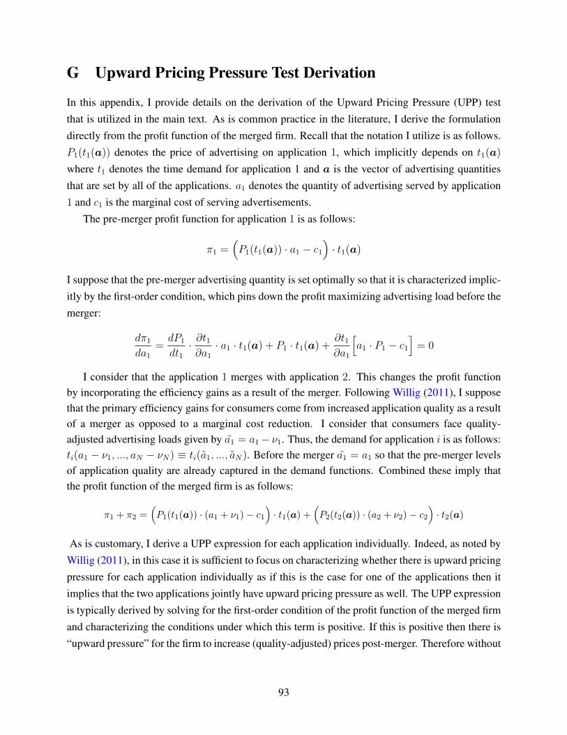
G Upward Pricing Pressure Test Derivation

In this appendix, I provide details on the derivation of the Upward Pricing Pressure (UPP) testthat is utilized in the main text. As is common practice in the literature, I derive the formulationdirectly from the profit function of the merged firm. Recall that the notation I utilize is as follows.P1(t1(a)) denotes the price of advertising on application 1, which implicitly depends on t1(a)

where t1 denotes the time demand for application 1 and a is the vector of advertising quantitiesthat are set by all of the applications. a1 denotes the quantity of advertising served by application1 and c1 is the marginal cost of serving advertisements.

The pre-merger profit function for application 1 is as follows:

π1 =(P1(t1(a)) · a1 − c1

)· t1(a)

I suppose that the pre-merger advertising quantity is set optimally so that it is characterized implic-itly by the first-order condition, which pins down the profit maximizing advertising load before themerger:

dπ1da1

=dP1

dt1· ∂t1∂a1· a1 · t1(a) + P1 · t1(a) +

∂t1∂a1

[a1 · P1 − c1

]= 0

I consider that the application 1 merges with application 2. This changes the profit functionby incorporating the efficiency gains as a result of the merger. Following Willig (2011), I supposethat the primary efficiency gains for consumers come from increased application quality as a resultof a merger as opposed to a marginal cost reduction. I consider that consumers face quality-adjusted advertising loads given by a1 = a1− ν1. Thus, the demand for application i is as follows:ti(a1 − ν1, ..., aN − νN) ≡ ti(a1, ..., aN). Before the merger a1 = a1 so that the pre-merger levelsof application quality are already captured in the demand functions. Combined these imply thatthe profit function of the merged firm is as follows:

π1 + π2 =(P1(t1(a)) · (a1 + ν1)− c1

)· t1(a) +

(P2(t2(a)) · (a2 + ν2)− c2

)· t2(a)

As is customary, I derive a UPP expression for each application individually. Indeed, as noted byWillig (2011), in this case it is sufficient to focus on characterizing whether there is upward pricingpressure for each application individually as if this is the case for one of the applications then itimplies that the two applications jointly have upward pricing pressure as well. The UPP expressionis typically derived by solving for the first-order condition of the profit function of the merged firmand characterizing the conditions under which this term is positive. If this is positive then there is“upward pressure” for the firm to increase (quality-adjusted) prices post-merger. Therefore without

93

loss of generality I focus on the first-order condition for application 1.

∂π1∂a1

=dP1

dt1· ∂t1∂a1· a1 · t1(a) + P1 · t1(a) +

∂t1∂a1

[a1 · P1 − c1

]︸ ︷︷ ︸

=0 at pre-merger

+dP1

dt1· ∂t1∂a1· ν1 · t1(a) +

∂t1∂a1· ν1 · P1

+∂t2∂a1· (P2 · (a2 + ν2)− c2) +

dP2

dt2· ∂t2∂a1· t2(a) · (a2 + ν2) = 0

The term noted in the brackets corresponds to the first-order condition of application 1 which,at the pre-merger advertising quantities, evaluates to 0. Recall that the diversion ratio is defined as

D12 ≡ −1 ·∂t2∂a1∂t1∂a1

. I divide the remaining terms through by −1 · ∂t1∂a1

and reorganize to obtain the

following UPP expression:

UPP1 = D12 ·(P2 · (a2 + ν2)− c2︸ ︷︷ ︸

Revenue from Diversion

+dP2

dt2· (a2 + ν2) · t2(a)︸ ︷︷ ︸

Price Change from Diversion

)−(ν1 ·

(dP1

dt1· t1(a) + P1

)︸ ︷︷ ︸

Quality Efficiency Gains

)

H Collection of Survey Responses

In this section are the responses to the optional question in the endline survey which asked theparticipants to describe in words how they responded to the restrictions.

• Addiction

– I hated it while it happened, but it really broke the app’s addictive nature.

– I never realized that I am tsuch addicting to instagram until I found myself opened itabsentmindedly several times during mY restrictions period. my usage time of ig hasdecreased from averagely 6.5 hrs before the restrictions to 3 hr in the first week, butbounce back to 7 hrs this week, even exceeding the number before.

– It’s strange, because it didn’t feel like I needed YouTube, I just knew I had spent a lotof time on it. However, when it became restricted, I noticed how much time I had spentsimply laying about and watching YouTube. It felt weird knowing that my instinct wasto immediately press the YouTube button when I got bored, and I realized I perhapsneed/use it more than I think.

– It was crazy how addicted I am to these apps. During the restrictions, I kept accidentallytrying to open the app -all the time. I didn’t realize how much time I spent on them.

– I kept opening instagram time after time forgetting that is was blocked

94

– I had one restriction on Instagram and it was weird breaking the habit of accessing andtook some getting used to avoiding the app

– When the restriction started I got a feeling I was gonna be a little anxious. I was wrong.

– It was frustrating - did not know I was so addicted to YouTube

– I felt out of the loop so I often tried to access Instagram using my laptop.

– At first restricting instagram was frustrating as i had the application on my home screenand built muscle memory for the past 4 years to press that part of the screen where theinstagram shortcut is. I removed instagram from my home screen and after 5 days ofthe restriction i completely realized instagram was nor important at all for me and onlytime i open it is when i receive a direct message.

• Shifted Towards Other Apps

– It wasn’t easy at first as I tried to access the restricted application about two differenttimes but I received the restriction message from screen time app with a grin on myface....lol. I had to figure out what I want from other applications I didn’t know offeredsimilar content before time, after the restriction elapsed, I had adjusted to sourcing forsuch content on both apps.

– Well at first after my YouTube was restricted, I thought I could access it using mybrowser but then i realised that was also impossible. I was like, how will I cope withoutstreaming videos on YouTube? But after some time I adjusted and got used to it.

– At the beginning i felt like damn this is an important application (Youtube) and whatif i need it for anything Turns out i dont need it as much and there are other optionsavailable

– Pre-COVID, I would listen to a lot of podcasts when driving, walking to class, etc.So when Youtube was restricted, I mostly just listened to more podcasts like I usedto. I think I also probably watched more Youtube on my PC and smart TV during thisperiod.

– At the beginning it felt like something was missing but eventually I started using otherapps and filled that vacancy

– I spent time on twitch watching streamers vs. Youtube where I had watched thembefore.

– I think the restriction gave me the opportunity to spend more time on other applicationsi had already installed but hardly use.

95

– I often use youtube for music on my phone when I don’t want to pay for Spotify pre-mium, but during the restriction period I ended up resubscribing to Spotify Premiumfor $5 so I could listen to music on my phone easily

• Realized Value of Application

– It was a bit hard to adapt at first but I eventually got used to it.Eventually I realized I ambetter off without it so I ended up deleting it and till now am okay with my decision.

– After the restriction I definitely started spending more time on the app that was re-stricted. I started to use the app more because I wanted to track local businesses whichcan be hard to discover by googling. I’m not sure if it was a coincidence that I de-veloped an interest in small businesses and increased my app usage or if it was therestriction that caused me to appreciate what I could do on the app more.

– I felt that I missed using it I realized I was spending to much time on the app

– Struggling to access Instagram, but when there’s no restrictions, i found that the contenti wanna access previously is very trivial

– I felt minorly inconvenienced since I could still access on my computer if it were anemergency like an insta dm I needed to respond to. Having time away from instadefinitely helped me mentally.

– Sometimes I misses to use but nothing as bad as I thought. Most of time I have notimportante to do, Its just a way to spend time

– I felt after restrictions that I need this application more and I can’t take this restrictionsfor a long.

– YouTube was restricted, so it was a little difficult when my baby was having a meltdownin public, but it also wasn’t as often as usual, thankfully. It was difficult also if Ineeded to learn something off of YouTube pertaining to my career like a how-to or newtechnique.

• Shifted Towards Non-Digital Activities

– Honestly I spent more time outdoor and with friends.

– I initially felt bored, since a common reflex I had was to open up Youtube wheneverI had nothing to do. However, within a few days, I started doing other things instead,such as reading. It was actually a good experience.

– At first it was difficult because YouTube is the most used app by me.Whatever it isYouTube is a go to for me in my daily life.After that I made up my mind to concentrate

96

in different things and spent more time off the devices.I tried to concentrate more onmy studies and spent time with my family.

– I was surprised my youtube was restricted. For me its a big part of the content i consumeand it is was hard to not have it on my phone. Initially I tried watching it on mycomputer but it was something i couldn’t keep up all the time. Over time my useagedropped from watching a lot to, mainly watching when i am on my computer taking asmall break (even then only watching the videos i really like and not wasting time onYT)

• Impact on Socializing

– I realized I spent a lot of time on an app establishing really ineffective communication.I changed the way in which I communicate online.

– I didn’t think I used Instagram very much but the restriction turned out to be veryannoying as friends would message me there and wonder why I wasn’t responding

– I used Instagram to communicate with friends less frequently when it was restricted,but used WhatsApp more instead. These were reverted after restrictions were lifted

– I felt frustrated because I feel like I was missing out. I wasn’t able to keep up with thepeople I followed on Instagram as much because the app was restricted

– I felt it was a very interesting experience. I don’t feel like I have an addiction to certainapplications and could probably live my life without it. The only limit I faced was thatI could not contact certain people, who I only talk with on that application. But tobe honest, I could live even without those conversations or certain people and wouldprobably find other apps to contact them on. But I did not do that.

– Instagram was restricted for me and because I mainly use it as a communication app, Iwas not significantly affected. I just used regular text, video call, and Snapchat to keepup socially.

– It was a little annoying especially whenever my friend shared something that can onlyopen on that platform. But after a couple of days I was able to make my peace with it

– I did a bit of communication on Instagram, so told the person I was chatting to to switchand that didn’t really happen so it ended up reducing how much we messaged

97