drifts and volatilities: monetary policies and outcomes in ... · drifts and volatilities: monetary...

Drifts and Volatilities: Monetary Policies andOutcomes in the Post WWII U.S.∗

Timothy CogleyArizona State University

Thomas J. Sargent

New York University and Hoover Institution

Revised: August 2002

Abstract

For a VAR with drifting coefficients and stochastic volatilities, wepresent posterior densities for several objects that are of interest fordesigning and evaluating monetary policy. These include measures ofinflation persistence, the natural rate of unemployment, a core rateof inflation, and ‘activism coefficients’ for monetary policy rules. Ourposteriors imply substantial variation of all of these objects for postWWII U.S. data. After adjusting for changes in volatility, persis-tence of inflation increases during the 1970s then falls in the 1980sand 1990s. Innovation variances change systematically, being sub-stantially larger in the late 1970s than during other times. Measuresof uncertainty about core inflation and the degree of persistence covarypositively. We use our posterior distributions to evaluate the powerof several tests that have been used to test the null of time-invarianceof autoregressive coefficients of VARs against the alternative of time-varying coefficients. Except for one test, we find that those tests havelow power against the form of time variation captured by our model.That one test also rejects time invariance in the data.

∗We are grateful to Jean Boivin, Mark Gertler, Sergei Morozov, Christopher Sims, andTao Zha for comments and suggestions.

1

1 Introduction

This paper extends the model of Cogley and Sargent (2001) to incorporatestochastic volatility and then reestimates it for post World War II U.S. datain order to shed light on the following questions. Have aggregate time seriesresponded via time-invariant linear impulse response functions to possiblyheteroskedastic shocks? Or is it more likely that the impulse responses toshocks themselves have evolved over time because of drifting coefficients orother nonlinearities? We present evidence that shock variances evolved sys-tematically over time, but that so did the autoregressive coefficients of VARs.One of our main conclusions is that much of our earlier evidence for driftingcoefficients survives after we take stochastic volatility into account. We useour evidence about drift and stochastic volatility to infer that monetary pol-icy rules have changed and that the persistence of inflation itself has driftedover time.

1.1 Time invariance versus drift

The statistical tests of Sims (1980, 1999) and Bernanke and Mihov (1998a,1998b) seem to affirm a model that contradicts our findings. They failedto reject the hypothesis of time-invariance in the coefficients of VARs forperiods and variables like ours. To shed light on whether our results areinconsistent with theirs, we examine the performance of various tests thathave been used to detect deviations from time invariance. Except for one, wefind that those tests have low power against our particular model of driftingcoefficients. And that one test actually rejects time invariance in the data.These results about power help reconcile our findings with those of Sims andBernanke and Mihov.

1.2 Bad policy or bad luck?

This paper accumulates evidence inside an atheoretical statistical model.1

But we use the patterns of time variation that our statistical model detectsto shed light on some important substantive and theoretical questions aboutpost WWII U.S. monetary policy. These revolve around whether it was badmonetary policy or bad luck that made inflation-unemployment outcomes

1By atheoretical we mean that the model’s parameters are not explicitly linked toparameters describing decision makers’ preferences and constraints.

2

worse in the 1970s than before or after. The view of DeLong (1997) andRomer and Romer (2002), which they support by stringing together inter-esting anecdotes and selections from government reports, asserts that it wasbad policy. Their story is that during the 1950s and early 1960s, the Fedbasically understood the correct model (which in their view incorporates thenatural rate theory that asserts that there is no exploitable trade off betweeninflation and unemployment); that Fed policy makers in the late 1960s andearly 1970s were seduced by Samuelson and Solow’s (1960) promise of anexploitable trade-off between inflation and unemployment; and that underVolcker’s leadership, the Fed came to its senses, accepted the natural ratehypothesis, and focused monetary policy on setting inflation low.

Aspects of this “Berkeley view” receive backing from statistical work byClarida, Gali, and Gertler (2000) and Taylor (1993), who fit monetary pol-icy rules for subperiods that they choose to illuminate possible differencesbetween the Burns and the Volcker-Greenspan eras. They find evidence fora systematic change of monetary policy across the two eras, a change thatin Clarida, Gali, and Gertler’s ‘new-neoclassical-synthesis’ macroeconomicmodel would lead to better inflation-unemployment outcomes.

But Taylor’s and Clarida, Gertler, and Gali’s interpretation of the datahas been disputed by Sims (1980, 1999) and Bernanke and Mihov (1998a,1998b), both of whom have presented evidence that the U.S. data do notprompt rejection of the time invariance of the autoregressive coefficients of aVAR. They also present evidence for shifts in the variances of the innovationsto their VARs. If one equation of the VAR is interpreted as describing amonetary policy rule, then Sims’s and Bernanke and Mihov’s results saythat it was not the monetary policy strategy but luck (i.e., the volatility ofthe shocks) that changed between the Burns and the non-Burns periods.

1.3 Inflation persistence and inferences about the nat-ural rate

The persistence of inflation plays an important role in some widely usedempirical strategies for testing the natural rate hypothesis and for estimatingthe natural unemployment rate. As we shall see, inflation persistence alsoplays an important role in lending relevance to instruments for estimatingmonetary policy rules. Therefore, we use our statistical model to portray theevolving persistence of inflation. We define a measure of persistence based on

3

the normalized spectrum of inflation at zero frequency, then present how thismeasure of persistence increased during the 1960s and 70s, then fell duringthe 1980s and 1990s.

1.4 Drifting coefficients and the Lucas Critique

Drifting coefficients have been an important piece of unfinished businesswithin macroeconomic theory since Lucas played them up in the first half ofhis 1976 Critique, but then ignored them in the second half.2 In AppendixA, we revisit how drifting coefficients bear on the theory of economic policyin the context of recent ideas about self-confirming equilibria. This appendixprovides background for a view that helps to bolster the time-invariance viewof the data taken by Sims and Bernanke and Mihov.

1.5 Method

We take a Bayesian perspective and report time series of posterior densitiesfor various economically interesting functions of hyperparameters and hiddenstates. We use a Markov Chain Monte Carlo algorithm to compute posteriordensities.

1.6 Organization

The remainder of this paper is organized as follows. Section 2 describesthe basic statistical model that we use to develop empirical evidence. Weconsign to appendix B a detailed description of the Markov Chain MonteCarlo algorithm that we use to approximate the posterior density of ourmodel. Section 3 reports our results, and section 4 concludes. Appendix Apursues a theme opened in the Lucas Critique about how drifting coefficientmodels bear on alternative theories of economic policy.

2See Sargent (1999) for more about this interpretation of the two halves of Lucas’s 1976paper.

4

2 A Bayesian Vector Autoregression with Drift-

ing Parameters and Stochastic Volatility

The object of Cogley and Sargent (2001) was to develop empirical evidenceabout the evolving law of motion for inflation and to relate the evidence tostories about changes in monetary policy rules. To that end, we fit a Bayesianvector autoregression for inflation, unemployment, and a short term interestrate. We introduced drifting VAR parameters, so that the law of motioncould evolve, but assumed the VAR innovation variance was constant. Thus,our measurement equation was

yt = X ′tθt + εt, (1)

where yt is a vector of endogenous variables, Xt includes a constant plus lagsof yt, and θt is a vector of VAR parameters. The residuals, εt, were assumedto be conditionally normal with mean zero and constant covariance matrixR.

The VAR parameters were assumed to evolve as driftless random walkssubject to reflecting barriers,

p(θt+1|θt, V ) ∝ I(θt+1)f(θt+1|θt, Q). (2)

The unrestricted transition density f(θt+1|θt, Q) represents a driftless randomwalk,

f(θt+1|θt, Q) ∼ N(θt, Q), (3)

so that θt evolves asθt = θt−1 + vt, (4)

apart from the reflecting barrier. The innovation vt is normal with meanzero and variance Q, and we allowed for correlation between the state andmeasurement innovations, cov(vt, εt) = C.

The reflecting barrier is encoded in the indicator function, I(θt), whichtakes a value of 0 when the roots of the associated VAR polynomial are insidethe unit circle and is equal to 1 otherwise. This is a stability condition forthe VAR, reflecting an a priori belief about the implausibility of explosiverepresentations for inflation, unemployment, and real interest. The stabilityprior follows from our belief that the Fed chooses policy rules in a purposefulway. Assuming that the Fed has a loss function that penalizes the variance

5

of inflation, it will not choose a policy rule that results in a unit root ininflation, for that results in an infinite loss.3

2.1 Sims’s and Stock’s criticisms

Sims (2001) and Stock (2001) were concerned that our methods might ex-aggerate the time variation in θt. One comment concerned the distinctionbetween filtered and smoothed estimates. Cogley and Sargent (2001) re-ported results based on filtered estimates, and Sims pointed out that thereis transient variation in filtered estimates even in time-invariant systems. Inthis paper, we report results based on smoothed estimates of θ.

More importantly, Sims and Stock questioned our assumption that Ris constant. They pointed to evidence developed by Bernanke and Mihov(1998a,b), Kim and Nelson (1999), McConnell and Perez Quiros (2000), andothers that VAR innovation variances have changed over time. Bernankeand Mihov focused on monetary policy rules and found a dramatic increasein the variance of monetary policy shocks between 1979 and 1982. Kim andNelson and McConnell and Perez Quiros studied the growing stability of theU.S. economy, which they characterize in terms of a large decline in VARinnovation variances after the mid-1980s. The reason for this decline is thesubject of debate, but there is now much evidence against our assumption ofconstant R.

Sims and Stock also noted that there is little evidence in the literatureto support our assumption of drifting θ. Bernanke and Mihov, for instance,used a procedure developed by Andrews (1993) to test for shifts in VARparameters and were unable to reject time invariance. Indeed, their preferredspecification was the opposite of ours, with constant θ and varying R.

If the world were characterized by constant θ and drifting R, and we

3To take a concrete example, consider the model of Rudebusch and Svennson (1999).Their model consists of an IS curve, a Phillips curve, and a monetary policy rule, andthey endow the central bank with a loss function that penalizes inflation variance. ThePhillips curve has adaptive expectations with the natural rate hypothesis being cast interms of Solow and Tobin’s unit-sum-of-the weights form. That form is consistent withrational expectations only when there is a unit root in inflation. The autoregressive rootsfor the system are not, however, determined by the Phillips curve alone; they also dependon the choice of monetary policy rule. With an arbitrary policy rule, the autoregressiveroots can be inside, outside, or on the unit circle, but they are stable under optimal ornear-optimal policies. When a shock moves inflation away from its target, poorly chosenpolicy rules may let it drift, but well-chosen rules pull it back.

6

fit an approximating model with constant R and drifting θ, then it seemslikely that our estimates of θ would drift to compensate for misspecificationof R, thus exaggerating the time variation in θ. Stock suggested that thismight account for our evidence on changes in inflation persistence. There ismuch evidence to support a positive relation between the level and varianceof inflation, but the variance could be high either because of large innovationvariances or because of strong shock persistence. A model with constant θand drifting R would attribute the high inflation variance of the 1970s to anincrease in innovation variances, while a model with drifting θ and constantR would attribute it to an increase in shock persistence. If Bernanke andMihov are right, the evidence on inflation persistence reported in Cogley andSargent (2001) paper may be an artifact of model misspecification.

2.2 Strategy for sorting out the issues

Of course, it is possible that both the coefficients and the volatilities vary, butmost empirical models focus on one or the other. In this paper, we develop anempirical model that allows both to vary. We use the model to consider theextent to which drift in R undermines our evidence on drift in θ, and also toconduct power simulations for the Andrews-Bernanke-Mihov test. Their nullhypothesis, which they were unable to reject, was that θ is time invariant.Whether this constitutes damning evidence against our vision of the worlddepends on the power of the test. Their evidence would be damning if thetest reliably rejected a model like ours, but not so damning otherwise.

To put both elements in motion, we retain much of the specification de-scribed above, but now we assume that the VAR innovations can be expressedas

εt = R1/2t ξt, (5)

where ξt is a standard normal random vector. Because we are complicatingthe model by introducing a drifting innovation variance, we simplify in an-other direction to economize on free parameters. Thus, we also assume thatstandardized VAR innovations are independent of parameter innovations,

E(ξtvs) = 0 for all t, s. (6)

To model drifting variances, we adopt a multivariate version of the stochas-tic volatility model of Jacquier, Polson, and Rossi (1994).4 In particular, we

4This formulation is closely related to the multi-factor stochastic volatility models of

7

assume that Rt can be expressed as

Rt = B−1HtB−1′, (7)

where Ht is diagonal and B is lower triangular,

Ht =

h1t 0 0

0 h2t 00 0 h3t

, (8)

B =

1 0 0

β21 1 0β31 β32 1

. (9)

The diagonal elements of Ht are assumed to be independent, univariatestochastic volatilities that evolve as driftless, geometric random walks,

ln hit = ln hit−1 + σiηit. (10)

The random walk specification is designed for permanent shifts in the inno-vation variance, such as those emphasized in the literature on the growingstability of the U.S. economy. The volatility innovations, ηit, are standardnormal random variables that are independent of one another and of theother shocks in the model, ξt and vt. The volatility innovations are eachscaled by a free parameter σi that determines their magnitude. The fac-torization in (7) and log specification in (10) guarantee that Rt is positivedefinite. The free parameters in B allow for correlation among the elementsof εt. The matrix B orthogonalizes εt, but it is not an identification scheme.

This specification differs from others in the literature that assume finite-state Markov representations for Rt. Our specification has advantages anddisadvantages relative to hidden Markov models. One advantage of the latteris that they permit jumps, whereas our model forces the variance to adjustcontinuously. An advantage of our specification is that it permits recurrent,permanent shifts in variance. Markov representations in which no state isabsorbing permit recurrent shifts, but the system forever switches betweenthe same configurations. Markov representations with an absorbing statepermit permanent shifts in variance, but such a shift can only occur once.

Aguilar and West (2001), Jacquier, Polson, and Rossi (1999), and Pitt and Shephard(1999).

8

Our specification allows permanent shifts to recur and allows new patternsto develop going forward in time.

We use Markov Chain Monte Carlo (MCMC) methods to simulate theposterior density.5 Let

Y T = [y′1, . . . , y′

T ]′ (11)

θT = [θ′1, . . . , θ′T ]′ (12)

and

HT =

h11 h21 h31

h12 h22 h32

... ... ...h1T h2T h3T

(13)

represent the history of data, VAR parameters, and stochastic volatilities upto date T, let σ = (σ1, σ2, σ3) stand for the standard deviations of the log-volatility innovations, and let β = [β21, β31, β32] represent the free parametersin B. The posterior density,

p(θT , Q, σ, β, HT | Y T ), (14)

summarizes beliefs about the model’s free parameters, conditional on priorsand the history of observations, Y T .

3 Empirical Results

3.1 Data

In order to focus on the influence of drift in R, we use the same data as inour earlier paper. Inflation is measured by the CPI for all urban consumers,unemployment by the civilian unemployment rate, and the nominal interestrate by the yield on 3-month Treasury bills. Inflation and unemploymentdata are quarterly and seasonally adjusted, and Treasury bill data are theaverage of daily rates in the first month of each quarter. The sample spansthe period 1948.1 to 2000.Q4. We work with VAR(2) representations fornominal interest, inflation, and the logit of unemployment.

5See appendix B for details.

9

3.2 Priors

The hyperparameters and initial states are assumed to be independent acrossblocks, so that the joint prior can be expressed as the product of marginalpriors,

p(θ0, h10, h20, h30, Q, β, σ1, σ2, σ3)

= p(θ0)p(h10)p(h20)p(h30)p(Q)p(β)p(σ1)p(σ2)p(σ3). (15)

Our prior for θ0 is a truncated Gaussian density,

p(θ0) ∝ I(θ0)f(θ0) = I(θ0)N(θ, P ). (16)

The mean and variance of the Gaussian piece are calibrated by estimatinga time-invariant vector autoregression using data for 1948.Q3-1958.Q4. Themean, θ, is set equal to the point estimate, and the variance, P , is its asymp-totic variance. Because the initial estimates are based on a short stretch ofdata, the location of θ0 is only weakly restricted.

The matrix Q is a key parameter because it governs the rate of drift in θ.We adopt an informative prior for Q, but we set its parameters to maximizethe weight that the posterior puts on sample information. Our prior for Q isinverse-Wishart,

p(Q) = IW (Q−1, T0), (17)

with degrees of freedom T0 and scale matrix Q. The degrees of freedom T0

must exceed the dimension of θt in order for this to be proper. To put aslittle weight as possible on the prior, we set

T0 = dim(θt) + 1. (18)

To calibrate Q, we assumeQ = γ2P (19)

and set γ2 = 3.5e-04. This makes Q comparable to the value used in Cogleyand Sargent (2001).6 This setting can be interpreted as a weak version of a‘business as usual’ prior, in the sense of Leeper and Zha (2001a,b). The prioris weak because it involves minimal degrees of freedom. It reflects a business-as-usual perspective because the implied values for Q result in little variation

6An earlier draft experimented with alternative values of γ that push Q toward zero,i.e. in the direction of less variation in θ. We found only minor sensitivity to changes inγ.

10

in θ. Indeed, had we calibrated Q = Q, or set T0 so that a substantial weightwas put on the prior, drift in posterior estimates of θ would be negligible.Thus, the setting for Q is conservative for our vision of the world.

The parameters governing priors for Rt are set more or less arbitrarily,but also very loosely, so that the data are free to speak about this feature aswell. The prior for hi0 is log-normal,

p(ln hi0) = N(ln hi, 10), (20)

where hi is the initial estimate of the residual variance of variable i. Noticethat a variance of 10 is huge on a natural log scale, making this weaklyinformative for hi0. Similarly, the prior for β is normal with a large variance,

p(β) = N(0, 10000 · I3). (21)

Finally, the prior for σ2i is inverse gamma with a single degree of freedom,

p(σ2i ) = IG(

.012

2,1

2). (22)

The specification is designed to put a heavy weight on sample information.

3.3 Details of the Simulation

We executed 100,000 replications of a Metropolis-within-Gibbs sampler anddiscarded the first 50,000 to allow for convergence to the ergodic distribu-tion. We checked convergence by inspecting recursive mean plots of variousparameters and by comparing results across parallel chains starting from dif-ferent initial conditions. Because the output files are huge, we saved every10th draw from the Markov chain, to economize on storage space. This hasa side benefit of reducing autocorrelation across draws, but it does increasethe variance of ensemble averages from the simulation. This yields a sampleof 5000 draws from the posterior density. The estimates reported below arecomputed from averages of this sample.

3.4 The Posterior Mean of Q

We begin with evidence on the rate of drift in θ, as summarized by posteriorestimates of Q. Recall that Q is the virtual innovation variance for VARparameters. Large values mean rapid movements in θ, smaller values imply

11

a slower rate of drift, and Q = 0 represents a time-invariant model. Thefollowing table addresses two questions, whether the results are sensitive tothe VAR ordering and how the stability prior influences the rate of drift inθ.

Table 1: Posterior Mean Estimates of Q

Stability Imposed Stability Not Imposed

VAR Orderings tr(Q) max(λ) tr(Q) max(λ)

i, π, u 0.055 0.025 0.056 0.027

i, u, π 0.047 0.023 0.059 0.031

π, i, u 0.064 0.031 0.082 0.044

π, u, i 0.062 0.031 0.088 0.051

u, i, π 0.057 0.026 0.051 0.028

u, π, i 0.055 0.024 0.072 0.035

Note: The headings tr(Q) and max(λ) refer to the trace of Q andto the largest eigenvalue.

Sims (1980) reported that the ordering of variables in an identified VARmattered for a comparison of interwar and postwar business cycles. In par-ticular, for one ordering he found minimal changes in the shape of impulseresponse functions, with most of the difference between interwar and postwarcycles being due to a reduction in shock variances. He suggested to us thatthe ordering of variables might matter in our model too because of the wayVAR innovation variances depend on the stochastic volatilities. In our spec-ification, the first and second variables share common sources of stochasticvolatility with the other variables, but the third variable has an independentsource of volatility. Shuffling the variables might alter estimates of VARinnovation variances.

Accordingly, we estimated all possible orderings to see whether thereexists an ordering that mutes evidence for drift in θ, as in Sims (1980). Thisseems not to be the case. With the stability condition imposed (our preferredspecification), there are only minor differences in posterior estimates of Q.The ordering that minimizes the rate of drift in θ is [it, ut, πt]

′, and theremainder of the paper focuses on this specification. This is conservative forour perspective, but results for the other orderings are similar.

12

The second question concerns how the stability prior influences drift inθ. One might conjecture that the stability constraint amplifies evidence fordrift in θ by pushing the system away from the unit root boundary, forcingthe model to fit inflation persistence via shifts in the mean. Again, thisseems not to be the case; posterior mean estimates for Q are smaller whenthe stability condition is imposed. Withdrawing the stability prior increasesthe rate of drift in θ.

The next table explores the structure of drift in θ, focusing on the minimum-Q ordering [i, u, π]′. Sargent’s (1999) learning model predicts that reducedform parameters should drift in a highly structured way, because of the cross-equation restrictions associated with optimization and foresight. A formaltreatment of cross-equation restrictions with parameter drift is a priorityfor future work. Here we report some preliminary evidence based on theprincipal components of Q.

Table 2: Principal Components of Q

Variance Percent of Total Variation1st PC 0.0230 0.4852nd PC 0.0165 0.8323rd PC 0.0054 0.9454th PC 0.0008 0.9635th PC 0.0007 0.978

Note: The second column reports the variance of the nth compo-nent (the nth eigenvalue of Q), and the third states the fraction ofthe total variation (trace of Q) for which the first n componentsaccount. The results refer to the minimum-Q ordering [i, u, π]′.

The table confirms that drift in θ is highly structured. There are 21 freeparameters in a trivariate VAR(2) model, but only three linear combinationsvary significantly over time. The first principal component accounts for al-most half the total variation, the first two components jointly account formore than 80 percent, and the first three account for roughly 95 percent.These components load most heavily on lags of nominal interest and unem-ployment in the inflation equation; they differ in the relative weights placedon various lags. The remaining principal components, and the coefficients in

13

the nominal interest and unemployment equations, are approximately timeinvariant. Thus the model’s departure from time invariance is not as greatas it first may seem. There are two or three drifting components in θ thatmanifest themselves in a variety of ways.

3.5 The Evolution of Rt

Next we consider evidence on the evolution of Rt. Figure 1 depicts the pos-terior mean of Rt for the minimal-Q ordering [i, u, π]′. The left-hand columnportrays standard deviations for VAR innovations, expressed in basis pointsat quarterly rates, and the right-hand column shows correlation coefficients.

The estimates support the contention that variation in Rt is an importantfeature of the data. Indeed, the patterns shown here resemble those reportedby Bernanke and Mihov, Kim and Nelson, McConnell and Perez Quiros, andothers.

For example, there is a substantial reduction in the innovation variancefor unemployment in the early 1980s. At that time, the standard deviationfell by roughly 40 percent, an estimate comparable to those of Kim andNelson and McConnell and Perez Quiros. Indeed, this seems to be part ofa longer-term trend of growing stability in unemployment innovations. Ourestimates suggest that there was a comparable decrease in variance in theearly 1960s and that the standard error has fallen by a total of roughly 60percent since the late 1950s. The trend toward greater stability

14

1960 1970 1980 1990 2000

20

40

60

Standard Error of Innovations

1960 1970 1980 1990 2000−0.3

−0.2

−0.1

Correlations

1960 1970 1980 1990 200030

40

50

60

1960 1970 1980 1990 2000

0.2

0.4

0.6

0.8

1960 1970 1980 1990 2000

3

4

5

6

1960 1970 1980 1990 2000

−0.25

−0.2

−0.15

−0.1

−0.05

NominalInterest

Inflation

Unemployment

Interest−Unemployment

Interest−Inflation

Inflation−Unemployment

Figure 1: Posterior Mean of Rt

was punctuated in the 1970s and early 1980s by countercyclical increases invariance. Whether the downward drift or business cycle pattern are likely torecur is an open question.

In addition, between 1979 and 1981, there is a spike in the innovationvariances for nominal interest and inflation. The spike in the innovationvariance for nominal interest resembles the estimates of Bernanke and Mihov.The two variances fell sharply after 1981 and reverted within a few years tolevels achieved in the 1960s.

The right-hand column illustrates the evolution of correlations amongthe VAR innovations, calculated from the posterior mean, E(Rt|T ). Unem-ployment innovations were negatively correlated with innovations in inflationand nominal interest throughout the sample. The correlations were largestin magnitude during the Volcker disinflation. At other times, the unem-ployment innovation was virtually orthogonal to the others. Inflation andnominal interest innovations were positively correlated throughout the sam-

15

ple, with the maximum degree of correlation again occurring in the early1980s.

This correlation pattern has some bearing on one strategy for identifyingmonetary policy shocks. McCallum (1999) has argued that monetary policyrules should be specified in terms of lagged variables, on the grounds that theFed lacks good current-quarter information about inflation, unemployment,and other target variables. This is especially relevant for decisions early inthe quarter. If the Fed’s policy rule depends only on lagged information,then it can be cast as the nominal interest equation in a VAR. Among otherthings, this means that nominal interest innovations are policy shocks andthat correlations among VAR innovations represent unidirectional causationfrom policy shocks to the other variables.

The signs of the correlations in figure 1 suggest that this interpretation isproblematic for our VAR. If nominal interest innovations were indeed policyshocks, conventional wisdom suggests they should be inversely correlatedwith inflation and positively correlated with unemployment, the opposite ofwhat we find. A positive correlation with inflation and a negative correlationwith unemployment suggests a policy reaction. There must be some missinginformation.7

Finally, figure 2 reports the total prediction variance, log |E(Rt|T )|. Fol-lowing Whittle (1953), we interpret this as a measure of the total uncertaintyentering the system at each date.

7Two possibilities come to mind. There may be omitted lagged variables, so that thenominal interest innovation contains a component that is predictable based on a larger in-formation set. The Fed may also condition on current-quarter reports of commodity pricesor long term bond yields that are correlated with movements in inflation or unemployment.

16

1960 1965 1970 1975 1980 1985 1990 1995 2000

−42

−41

−40

−39

−38

−37

log

det R

(t)

Figure 2: Total Prediction Variance

The smoothed estimates shown here are similar to the filtered estimatesreported in our earlier paper. Both suggest a substantial increase in short-term uncertainty between 1965 and 1981 and an equally substantial decreasethereafter. The increase in uncertainty seems to have happened in two steps,one occurring between 1964 and 1972 and the other between 1977 and 1981.Most of the subsequent decrease occurred in the mid-1980s, during the latteryears of Volcker’s term. This picture suggests that the growing stability ofthe economy may reflect a return to stability, though the earlier period ofstability proved to be short-lived.

3.6 The Evolution of θt

There is no question that variation in R is an interesting and importantfeature of the data, but does it alter the patterns of drift in θ documented inour earlier paper? Our main interests concern movements in core inflation,the natural rate of unemployment, inflation persistence, the degree of policyactivism, and how they relate to one another. Our interest in these featuresfollows from their role in stories about how changes in monetary policy mayhave contributed to the rise and fall of inflation in the 1970s and 1980s.

3.6.1 Core Inflation and the Natural Rate of Unemployment

The first set of figures depicts movements in core inflation and the naturalrate of unemployment, which are estimated from local linear approxima-

17

tions to mean inflation and unemployment, evaluated at the posterior mean,E(θt|T ). Write (1) in companion form as

zt = µt|T + At|T zt−1 + ut, (23)

where zt consists of current and lagged values of yt, µt|T contains the inter-cepts in E(θt|T ), and At|T contains the autoregressive parameters. By analogywith a time-invariant model, mean inflation at t can be approximated by

πt = sπ(I − At|T )−1µt|T , (24)

where sπ is a row vector that selects inflation from zt. Similarly, mean un-employment can be approximated as

ut = su(I − At|T )−1µt|T , (25)

where su selects unemployment from zt.Figures 3 portrays the evolution of πt and ut for the ordering [i, u, π]′. Two

features are worth noting. First, allowing for drift in Rt does not eliminateeconomically meaningful movements in core inflation or the natural rate. Onthe contrary, the estimates are similar to those in our earlier paper. Coreinflation sweeps up from around 1.5 percent in the early 1960s, rises to apeak of approximately 8 percent in the late 1970s, and then falls to a rangeof 2.5 to 3.5 percent through most of the 1980s and 1990s. The natural rateof unemployment also rises in the late 1960s and 1970s and falls after 1980.

Second, it remains true that movements in πt and ut are highly correlatedwith one another, in accordance with the predictions of Parkin (1993) andIreland (1999). The unconditional correlation is 0.748.

1960 1965 1970 1975 1980 1985 1990 1995 2000

0.02

0.03

0.04

0.05

0.06

0.07

Core InflationNatural Rate of Unemployment

Figure 3: Core Inflation and the Natural Rate of Unemployment

18

Table 3 and figures 4 and 5 characterize the main sources of uncertaintyabout these estimates. The table and figures are based on a method de-veloped by Sims and Zha (1999) for constructing error bands for impulseresponse functions. We start by estimating the posterior covariance matrixfor πt via the delta method,

Vπ =∂π

∂θVθ

∂π

∂θ′. (26)

Vθ is the KT x KT 8 covariance matrix for θT and ∂π/∂θ is the T x KT matrixof partial derivatives of the function that maps VAR parameters into coreinflation, evaluated at the posterior mean of θT . The posterior covarianceVθ is estimated from the ensemble of Metropolis draws, and derivatives werecalculated numerically.9

Vπ is a large object, and we need a tractable way to represent the infor-mation it contains. Sims and Zha recommend error bands based on the firstfew principal components.10 Let Vπ = WΛW ′, where Λ is a diagonal matrixof eigenvalues and W is an orthonormal matrix of eigenvectors. A two-sigmaerror band for the ith principal component is

πt ± 2λ1/2i Wi, (27)

where λi is the variance of the ith principal component and Wi is the ithcolumn of W.

Table 3 reports the cumulative proportion of the total variation for whichthe principal components account. The second column refers to Vπ, and thethird column decomposes the covariance matrix for the natural rate, Vu. Theother columns are discussed below.

8K is the number of elements in θ, and T represents the number of years. We focusedon every fourth observation to keep V to a manageable size.

9This roundabout method for approximating Vπ was used because the direct estimatewas contaminated by a few outliers, which dominated the principal components decompo-sition on which Sims-Zha bands are based. The outliers may reflect shortcomings of ourlinear approximations near the unit root boundary.

10If the elements of πt were uncorrelated across t, it would be natural to focus insteadon the diagonal elements of Vπ, e.g. by graphing the posterior mean plus or minus twostandard errors at each date. But πt is serially correlated, and Sims and Zha argue thata collection of principal components bands better represents the shape of the posterior insuch cases.

19

Table 3: Principal Component Decomposition for Sims-Zha Bands

Vπ Vu Vgππ VA

1st PC 0.521 0.382 0.374 0.6622nd PC 0.604 0.492 0.490 0.8013rd PC 0.674 0.597 0.561 0.8704th PC 0.715 0.685 0.612 0.9065th PC 0.750 0.727 0.662 0.9366th PC 0.778 0.767 0.701 0.9498th PC 0.822 0.820 0.756 0.97210th PC 0.851 0.856 0.800 0.984

Note: Entries represent the cumulative percentage of the totalvariation (trace of V ) for which the first n principal componentsaccount.

One interesting feature is the number of non-trivial components. Thefirst principal component in Vπ and Vu accounts for 40 to 50 percent of thetotal variation, and the first 5 jointly account for about 75 percent. Thissuggests an important departure from time invariance. In a time-invariantmodel, there would be a single factor representing uncertainty about thelocation of the terminal estimate, but smoothed estimates going backwardin time would be perfectly correlated with the terminal estimate and wouldcontribute no additional uncertainty.11 V would be a TxT matrix with rankone, and the single principal component would describe uncertainty aboutthe terminal location. In a nearly time-invariant model, i.e. one with smallQ, the path to the terminal estimate might wiggle a little, but one wouldstill expect uncertainty about the terminal estimate to dominate. That thefirst component accounts for a relatively small fraction of the total suggeststhere is also substantial variation in the shape of the path.

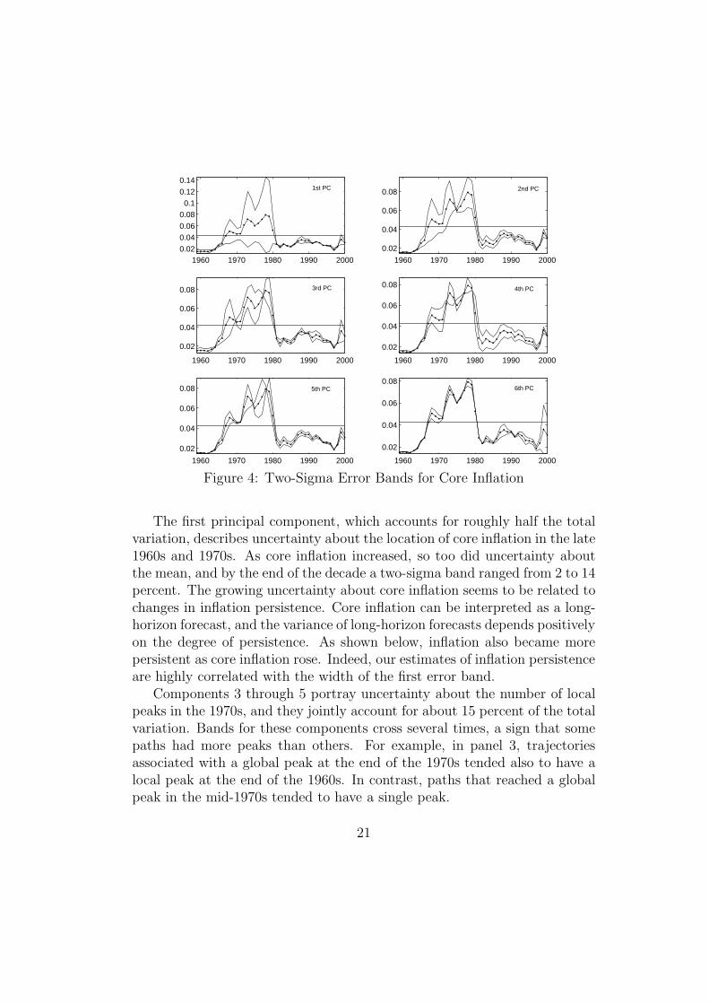
Error bands for core inflation are shown in figure 4. The central dottedline is the posterior mean estimate, reproduced from figure 3. The horizontalline is a benchmark, end-of-sample, time-invariant estimate of mean inflation.

11Setting Q = 0 in the Kalman filter implies Pt+1|t = Pt|t. Then the covariance matrixin the backward recursion of the Gibbs sampler would be Pt|t+1 = 0, implying a perfectcorrelation between draws of θt+1 and θt.

20

1960 1970 1980 1990 20000.02

0.04

0.06

0.08

0.1

0.12

0.14

1960 1970 1980 1990 2000

0.02

0.04

0.06

0.08

1960 1970 1980 1990 2000

0.02

0.04

0.06

0.08

1960 1970 1980 1990 2000

0.02

0.04

0.06

0.08

1960 1970 1980 1990 2000

0.02

0.04

0.06

0.08

1960 1970 1980 1990 2000

0.02

0.04

0.06

0.08

1st PC 2nd PC

3rd PC 4th PC

5th PC 6th PC

Figure 4: Two-Sigma Error Bands for Core Inflation

The first principal component, which accounts for roughly half the totalvariation, describes uncertainty about the location of core inflation in the late1960s and 1970s. As core inflation increased, so too did uncertainty aboutthe mean, and by the end of the decade a two-sigma band ranged from 2 to 14percent. The growing uncertainty about core inflation seems to be related tochanges in inflation persistence. Core inflation can be interpreted as a long-horizon forecast, and the variance of long-horizon forecasts depends positivelyon the degree of persistence. As shown below, inflation also became morepersistent as core inflation rose. Indeed, our estimates of inflation persistenceare highly correlated with the width of the first error band.

Components 3 through 5 portray uncertainty about the number of localpeaks in the 1970s, and they jointly account for about 15 percent of the totalvariation. Bands for these components cross several times, a sign that somepaths had more peaks than others. For example, in panel 3, trajectoriesassociated with a global peak at the end of the 1970s tended also to have alocal peak at the end of the 1960s. In contrast, paths that reached a globalpeak in the mid-1970s tended to have a single peak.

21

Finally, the sixth component loads heavily on the last few years in thesample, describing uncertainty about core inflation in the late 1990s. At theend of 2000, a two-sigma band for this component ranged from approximately1 to 5 percent.

1960 1970 1980 1990 20000.04

0.06

0.08

0.1

1960 1970 1980 1990 2000

0.04

0.05

0.06

0.07

1960 1970 1980 1990 20000.03

0.04

0.05

0.06

1960 1970 1980 1990 20000.03

0.04

0.05

0.06

1960 1970 1980 1990 2000

0.04

0.05

0.06

0.07

1960 1970 1980 1990 20000.04

0.05

0.06

0.07

1st PC 2nd PC

3rd PC 4th PC

5th PC 6th PC

Figure 5: Two-Sigma Error Bands for the Natural Rate of Unemployment

Error bands for the natural rate are constructed in the same way, and theyare shown in figure 5. Once again, the central dotted line is the posteriormean estimate, and the horizontal line is an end-of-sample, time-invariantestimate of mean unemployment. The first principal component in Vu alsocharacterizes uncertainty about the 1970s. The error band widens in the late1960s when the natural rate began to rise, and it narrows around 1980 whenthe mean estimate fell. The band achieved its maximum width around thetime of the oil shocks, when it ranged from roughly 4 to 11 percent. Thewidth of this band also seems to be related to changes in the persistence ofshocks to unemployment.

The second, third, and fourth components load heavily on the other yearsof the sample, jointly accounting for about 30 percent of the total variation.

22

Roughly speaking, they cover intervals of plus or minus 1 percentage pointaround the mean. The fifth and sixth components account for 8 percent ofthe variation, and they seem to be related to uncertainty about the timingand number of peaks in the natural rate.

3.6.2 Inflation Persistence

Next we turn to evidence on the evolution of second moments of inflation.Second moments are measured by a local linear approximation to the spec-trum for inflation,

fππ(ω, t) = sπ(I − At|T e−iω)−1E(Rt|T )

2π(I − At|T eiω)−1′sπ

′. (28)

evaluated at the posterior mean of θ and R. An estimate of fππ(ω, t) is shownin figure 6. Time is plotted on the x-axis, frequency on the y-axis, and poweron the z-axis.

0

0.116

0.233

0.349

0.4651960

1970

1980

1990

2000

0

0.2

0.4

0.6

0.8

1

1.2

1.4

1.6

1.8

x 10−3

YearCycles per Quarter

Pow

er

Figure 6: Spectrum for Inflation

Again, the estimates are similar to those reported in Cogley and Sargent(2001). The introduction of drift in Rt does not undermine our evidence onvariation in the spectrum for inflation.

The most significant feature of this graph is the variation over time inthe magnitude of low frequency power. In our earlier paper, we interpreted

23

the spectrum at zero as a measure of inflation persistence. Here that inter-pretation is no longer quite right, because variation in low-frequency powerdepends not only on drift in the autoregressive parameters, At|T , but also onmovements in the innovation variance, E(Rt|T ). In this case, the normalizedspectrum,

gππ(ω, t) =fππ(ω, t)∫ π

−πfππ(ω, t)dω

, (29)

provides a better measure of persistence. The normalized spectrum is thespectrum divided by the variance in each year. The normalization adjustsfor changes in innovation variances and measures autocorrelation rather thanautocovariance. We interpret gππ(0, t) as a measure of inflation persistence.

Estimates of the normalized spectrum are shown in figure 7. As in figure6, the dominant feature is the variation over time in low-frequency power,though the variation in gππ(0, t) differs somewhat from that in fππ(0, t). In-stead of sharp spikes in the 1970s, gππ(0, t) sweeps gradually upward in thelatter half of the 1960s and remains high throughout the 1970s. The spectrumat zero falls sharply after 1980, and there is discernible variation throughoutthe remainder of the sample.

0

0.116

0.233

0.349

0.4651960

1970

1980

1990

2000

0

1

2

3

4

5

YearCycles per Quarter

Pow

er

Figure 7: Normalized Spectrum for Inflation

Figure 8 depicts two-sigma error bands for gππ(0, t), based on the principalcomponents of its posterior covariance matrix, Vgππ . The latter was estimated

24

in the same way as Vπ or Vu. The third column in table 3 indicates that thefirst component in Vgππ accounts for only 37 percent of the total variationand that the first 5 components jointly account for 84 percent. Again, thissignifies substantial variation in the shape of the path for gππ(0, t).

1960 1970 1980 1990 2000

2

4

6

8

10

1960 1970 1980 1990 2000

2

4

6

8

10

12

1960 1970 1980 1990 2000

2

4

6

1960 1970 1980 1990 2000

2

4

6

1960 1970 1980 1990 2000

2

4

6

1960 1970 1980 1990 2000

2

4

6

1st PC 2nd PC

3rd PC 4th PC

5th PC 6th PC

Figure 8: Two-Sigma Error Bands for the Normalized Spectrum At Zero

Error bands for the first two components load heavily on the 1970s. Al-though the bands suggest there was greater persistence than in the early1960s or mid-1990s, the precise magnitude of the increase is hard to pindown. Roughly speaking, error bands for the first two components suggestthat gππ(0, t) was somewhere between 2 and 10. For the sake of compari-son, a univariate AR(1) process with coefficients of 0.85 to 0.97 has valuesof gππ(0) in this range. In contrast, the figure suggests that inflation wasapproximately white noise in the early 1960s and not far from white noise inthe mid-1990s. Uncertainty about inflation persistence was increasing againat the end of the sample.

The third, fourth, and fifth components reflect uncertainty about thetiming and number of peaks in gππ(0, t). For example, panels 3 and 5 suggest

25

that paths on which there was a more gradual increase in persistence tendedto have a big global peak in the late 1970s, while those on which there was amore rapid increase tended to have comparable twin peaks, first in the late1960s and then again in 1980. Panel 4 suggests that some paths had twinpeaks at the time of the oil shocks, while others had a single peak in 1980.These components jointly account for about 17 percent of the total variation.

One of the questions in which we are most interested concerns the rela-tion between inflation persistence and core inflation. In Cogley and Sargent(2001), we reported evidence of a strong positive correlation. Here we alsofind a strong positive correlation, equal to 0.92.

1960 1965 1970 1975 1980 1985 1990 1995 2000

1

2

3

4

5

6

7

Core Inflation (x 100)Normalized Spectrumat Zero

Figure 9: Core Inflation and Inflation Persistence

The relation between the two series is illustrated in figure 9, which re-produces estimates from figures 3 and 7. As core inflation rose in the 1960sand 1970s, inflation also became more persistent. Both features fell sharplyduring the Volcker disinflation. This correlation is problematic for the es-cape route models of Sargent (1999) and Cho, Williams, and Sargent (2002),which predict that inflation persistence grows along the transition from highto low inflation. Our estimates suggest the opposite pattern.

3.6.3 Monetary Policy Activism

Finally, we consider evidence on the evolution of policy activism. FollowingClarida, Gali, and Gertler (2000), we estimate this from a forward-lookingTaylor rule with interest smoothing,

it = β0 + β1Etπt,t+hπ + β2Etut,t+hu + β3it−1 + ηt, (30)

26

where πt,t+hπ represents average inflation from t to t+hπ and ut,t+hu is averageunemployment. The activism parameter is defined as

A = β1(1 − β3)−1, (31)

and the policy rule is said to be activist if A ≥ 1. With a Ricardian fiscal pol-icy, an activist monetary rule delivers a determinate equilibrium. Otherwise,sunspots may matter for inflation and unemployment.

We interpret the parameters of the policy rule as projection coefficientsand compute projections from our VAR. This is done via two-stage leastsquares on a date-by-date basis. The first step involves projecting the Fed’sforecasts Etπt,t+hπ and Etut,t+hu onto a set of instruments, and the secondinvolves projecting current interest rates onto the fitted values. At each date,we parameterize the VAR with posterior mean estimates of θt and Rt andcalculate population projections associated with those values.

The instruments chosen for the first-stage projection must be elements ofthe Fed’s information set. Notice that a complete specification of their infor-mation set is unnecessary; a subset of their conditioning variables is sufficientfor forming first-stage projections, subject of course to the order conditionfor identification. Among other variables, the Fed observes lags of inflation,unemployment, and nominal interest when making current-quarter decisions,and we project future inflation and unemployment onto a constant and twolags of each. Thus, our instruments for the Fed’s forecasts Etπt,t+hπ andEtut,t+hu are the VAR forecasts Et−1πt,t+hπ and Et−1ut,t+hu, respectively.12

Because θt and Rt evolve over time, so too do the policy projections.Point estimates for A are shown in figure 10. Here we assume hπ = 4 andhu = 2, but the results for one-quarter ahead forecasts are similar.

The estimates broadly resemble those reported by Clarida, et. al., as wellas those in our earlier paper. The estimated policy rule was activist in theearly 1960s, but became approximately neutral in the late 1960s and thenturned passive in the early 1970s. It remained passive until the early 1980s.The estimate of A rose sharply around the time of the Volcker disinflation,and it has remained in the activist region ever since. As shown in figure 11,

12Here we follow McCallum, who warns against the assumption that the Fed sees currentquarter inflation and unemployment when making decisions. This strategy also sidestepsassumptions about how to orthogonalize current quarter innovations. This is an importantadvantage of the Clarida, et. al. approach relative to structural VAR methods. Estab-lishing that the Fed can observe some variables is easier than compiling a complete list ofwhat the Fed sees.

27

the estimates of A are inversely related to core inflation and the degree ofinflation persistence, suggesting that changes in the degree of activism mayhave contributed to the rise and fall of inflation.

1955 1960 1965 1970 1975 1980 1985 1990 1995 2000 20050

2

4

6

8

10

12

Figure 10: Estimates of the Activism Coefficient

0 2 4 6 8 100.01

0.02

0.03

0.04

0.05

0.06

0.07

0.08

Cor

e In

flatio

n

Policy Activism0 2 4 6 8 10

0

1

2

3

4

5

6

Nor

m. S

pect

rum

at Z

ero

Policy Activism

corr = −0.72 corr = −0.79

Figure 11: Policy Activism, Core Inflation, and Inflation Persistence

Figure 12 suggests, however, that some qualifications are necessary, espe-cially at the beginning and end of the sample. The figure portrays two-sigmaerror bands based on the principal components of the posterior covariancematrix, VA. The last column of table 3 shows that several principal com-ponents contribute to VA, with the first component accounting for about

28

two-thirds of the total variation. That there is more than one importantcomponent is evidence for variation in the path of A.

1960 1980 2000

−20

0

20

40

1960 1980 2000

−10

0

10

20

30

1960 1980 2000

0

5

10

15

1960 1980 2000

0

5

10

1960 1980 2000

0

5

10

1960 1980 2000

0

5

10

1960 1980 2000

2

4

6

8

1960 1980 2000

2

4

6

8

1960 1980 2000

2

4

6

8

1st PC 2nd PC 3rd PC

4th PC 5th PC 6th PC

7th PC 8th PC 9th PC

Figure 12: Two-Sigma Error Bands for the Activism Parameter

But the shape of the path is well determined only in the middle of thesample. The first four principal components record substantial uncertainty atthe beginning and end. We interpret this as a symptom of weak identification.Substantial uncertainty about A occurs at times when inflation is weaklypersistent. Our instruments have little relevance when future inflation isweakly correlated with lagged variables, and the policy rule parameters areweakly identified at such times. Thus, inferences about A are fragile atthe beginning and end of the sample. There is better evidence of changesin A during the middle of the sample. Lagged variables are more relevantas instruments for the 1970s, when inflation and unemployment were verypersistent, and for that period the estimates are more precise.

29

The next figure characterizes more precisely how the posterior for At dif-fers across the Burns and Volcker-Greenspan terms. It illustrates histogramsfor At for the years 1975, 1985, and 1995. The histograms were constructedby calculating an activism parameter for each draw of θt and Rt in our simu-lation, for a total of 5000 in each year.13 Values for 1975 are shown in black,those for 1985 are in white, and estimates for 1995 are shown in yellow.

In 1975, the probability mass was concentrated near 1, and the probabilitythat At > 1 was 0.208. By 1985, the center of the distribution had shiftedto the right, and the probability that At > 1 had increased to 0.919. Thedistribution for 1995 is

−4 −2 0 2 4 6 8 10 120

500

1000

1500

2000

2500

3000

3500

4000

4500

Activism Parameter

197519851995

Figure 13: Histograms for At in Selected Years

similar to that for 1985, with a 0.941 probability that At > 1. Comparingestimates along the same sample paths, the probability that At increasedbetween 1975 and 1985 is 0.923, and the probability that it increased between1975 and 1995 is 0.943.

The estimates seem to corroborate those reported by Clarida, et. al.that monetary policy was passive in the 1970s and activist for much of theVolcker-Greenspan era. Estimates for the latter period are less precise, butit seems clear that the probability distribution for At shifted to the right.

13Outliers are collected in the end bins.

30

3.7 Tests for θ Stability

Finally, we consider classical tests for variation in θ. Bernanke and Mihov(1998a,b) were also concerned about the potential for shifts in VAR param-eters arising from changes in monetary policy, and they applied a test devel-oped by Andrews (1993) to examine stability of θ. For reduced form vectorautoregressions similar to ours, they were unable to reject the hypothesis oftime invariance.

We applied the same test to our data and found the same results. Weconsidered two versions of Andrews’s sup-LM test, one that examines pa-rameter stability for the VAR as a whole and another that tests stabilityon an equation-by-equation basis. The results are summarized in table 4.Columns labelled with variable names refer to single-equation tests, and thecolumn labelled ‘VAR’ refers to a test for the system as a whole. In eachcase, we fail to reject that θ is time invariant.14

Bernanke and Mihov correctly concluded that the test provides little ev-idence against stability of θ. But does the result constitute evidence againstparameter instability? A failure to reject provides evidence against an alter-native hypothesis only if it has reasonably high power. Whether this test hashigh power against a model like ours is an open question, so we decided toinvestigate it.

Table 4: Andrews’s sup-LM Test

Nominal Interest Unemployment Inflation VARData F F F FPower 0.136 0.172 0.112 0.252

Note: An ‘F’ means the test fails to reject at the 10 percent level whenapplied to actual data. Entries in the second row refer to the fractionof artificial samples in which the null hypothesis is rejected at the 5percent level.

To check the power of the test, we performed a Monte Carlo simulationusing our drifting parameter VAR as a data generating process. To generate

14We also performed a Monte Carlo simulation to check the size of the Andrews test;the results confirmed that size distortions do not explain the failure to reject.

31

artificial data, we parameterized equation (1) with draws of θT , HT , andB from the posterior density. For each draw of (θT , HT , B), we generatedan artificial sample for inflation, unemployment, and nominal interest andthen calculated the sup-LM statistics. We performed 10,000 replications andcounted the fraction of samples in which the null hypothesis of constant θis rejected at the 5 percent level. The results are summarized in the secondrow of table 4.

The power of the test is never very high. The VAR test has highest thesuccess rate, detecting drift in θ in about one-fourth of the samples. Thedetection probabilities are lower in the single equation tests, which reject atthe 5 percent level in only about 14 percent of the samples. Thus, even whenθ drifts in the way we describe, a failure to reject is at least 3 times as likelyas a rejection.

Andrews’s test is designed to have power against alternatives involving asingle shift in θ at some unknown break date. The results of this experimentmay just reflect that this test is less well suited to detect alternatives suchas ours that involve continual shifts in parameters. Accordingly, we alsoinvestigate a test developed by Nyblom (1989) and Hansen (1992) that isdesigned to have power against alternatives in which parameters evolve asdriftless random walks. Results for the Nyblom-Hansen test are summarizedin table 5.

Table 5: The Nyblom-Hansen Test

Nominal Interest Unemployment Inflation VARData F F F FPower 0.076 0.170 0.086 0.234

See the note to table 4.

When applied to actual data, the Nyblom-Hansen test also fails to rejecttime invariance for θ. To examine its power, we conducted another MonteCarlo simulation using our drifting parameter VAR as a data generatingmechanism, and we found that this test also has low power against our rep-resentation. Indeed, the detection probabilities are a bit lower than those forthe sup-LM test.

Boivin (1999) conjectures that the sup-Wald version of Andrews’s testmay have higher power than the others, and so we also consider this pro-cedure. The results, which are shown in table 6, provide some support for

32

his conjecture. The detection probability is higher in each case, and it issubstantially higher for the inflation equation. Indeed, this is the only caseamong the ones we study in which the detection probability exceeds 50 per-cent. It is noteworthy that in this case we also strongly reject time invariancein the actual data. Time invariance is also rejected for the VAR as a whole.

Table 6: Andrews’s sup-Wald Test

Nominal Interest Unemployment Inflation VARData F F R 1% R 5%Power 0.173 0.269 0.711 0.296

Note: ‘R x%’ signifies a rejection at the x percent level.

We made two other attempts to concentrate power in promising direc-tions. The first focuses on parameters of the Clarida, et. al. policy rule. Ifdrift in θ is indeed a manifestation of changes in monetary policy, then testsfor stability of the latter should be more powerful than for stability of theformer. The vector θ has high dimension, and the drifting components in θshould lie in a lower-dimensional subspace corresponding to drifting policyparameters.15 To test stability of the Clarida, et. al. rule, we estimated aversion for the period 1959-2000 using our data and instruments, and calcu-lated Andrews’s statistics.16 Perhaps surprisingly in light of their results, thetests fail to reject time invariance (see table 7). We repeated the procedurefor artificial samples generated from our VAR to check the power of the test.Once again, the results show that the tests have low detection probabilities.

Table 7: Stability of the CGG Policy Rule

sup-LM sup-WaldData F FPower 0.143 0.248


15This assumes that shifts in policy are the only source of drift in θ.16We chose Andrews’s tests because the CCG rule is estimated by GMM. The Nyblom-

Hansen test is based on ML estimates.

33

We also tried to increase power by concentrating on a single linear combi-nation of θ that we think is most likely to vary. The linear combination withgreatest variance is the first principal component, and we used the dominanteigenvector of the sample variance of E(∆θt|T ) to measure this component.As figures 14 and 15 illustrate, the first principal component dominates thevariation in θt|T ;17 most of the other principal components are approximatelytime invariant. The first component is also highly correlated with variationin the features discussed above. Thus it seems to be a promising candidateon which to concentrate.

1955 1960 1965 1970 1975 1980 1985 1990 1995 2000 2005−1.5

−1

−0.5

0

0.5

1

1.5

2

2.5

3

Figure 14: Principal Components of θt|T

17More precisely, the figures illustrate partial sums of the first principal component for∆θt|T .

34

0.5 1 1.5 2 2.50

0.02

0.04

0.06

0.08

0.11st PC−Core Inflation

0.5 1 1.5 2 2.50

1

2

3

4

5

61st PC−Norm. Spectrum

0.5 1 1.5 2 2.50.035

0.04

0.045

0.05

0.055

0.06

0.065

0.071st PC−Natural Rate

0.5 1 1.5 2 2.50

0.5

1

1.5

2

2.5

3

3.51st PC−Activism

corr = 0.96 corr = 0.86

corr = 0.71 corr = −0.82

Figure 15: Correlation of First Principal Component with Other Features

Yet the results of a Monte Carlo simulation, shown in table 8, suggestthat power remains low, with a rejection probability of only about 15 per-cent. Indeed, the procedure is inferior to the VAR tests reported above.Agnosticism about drifting components in θ seems to be better. Despite thelow power, one of the tests rejects time invariance in actual data.

Table 8: Stability of the First Principal Component

sup-LM sup-WaldData F R 5%Power 0.220 0.087


To summarize, most of our tests fail to reject time invariance of θ, butmost also have low power to detect the patterns of drift we describe above.In the one case where a test has a better-than-even chance of detecting driftin θ, for the data time invariance is rejected at better than the one-percentlevel. One reasonable interpretation is that θ is drifting, but that most ofthe procedures are unable to detect it.

35

Perhaps low power should not be a surprise. Our model nests the null oftime invariance as a limiting case, i.e. when Q = 0. One can imagine indexinga family of alternative models in terms of Q. For Q close to zero, size andpower should be approximately the same. Power should increase as Q getslarger, and eventually the tests are likely to reject with high probability.But in between there is a range of alternative models, arrayed in terms ofincreasing Q, that the tests are unlikely to reject. The message of the MonteCarlo detection statistics is that a model such as ours with economicallymeaningful drift in θ often falls in the indeterminate range.

4 Conclusion

One respectable view is that either an erroneous model, insufficient patience,or his inability to commit to a better policy made Arthur Burns respondto the end of Bretton Woods by administering monetary policy in a waythat produced the greatest peace time inflation in U.S. history; and thatan improved model, more patience, or greater discipline led Paul Volcker toadminister monetary policy in a way that conquered American inflation.18

Another respectable view is that what distinguished Burns and Volcker wasnot their models or policies but their luck. This paper and its predecessor(Cogley and Sargent (2001)) fit time series models that might help distinguishthese views.

This paper also responds to Sims’s (2001) and Stock’s (2001) criticism ofthe evidence for drifting systematic parts of vector autoregressions in Cogleyand Sargent (2001) by altering our specification to include stochastic volatil-ity. While we have found evidence for drifting variances within our newspecification, we continue to find evidence that the VAR coefficients havedrifted, mainly along one important direction. Our model is atheoretical,but for reasons discussed in Appendix A and also by Sargent (1999) andLuca Benati (2001), the presence of drifting coefficients contains clues aboutwhether government policy makers’ models or preferences have evolved overtime.

It is appropriate to be cautious in accepting evidence either for or againstdrifting coefficients. For reasons that are most clear in continuous time (seeAnderson, Hansen, and Sargent (2000)), it is much more difficult to detectevidence for movements in the systematic part of a vector autoregression

18See J. Bradford DeLong (1997) and John Taylor (1997).

36

than it is to detect stochastic volatility. This situation is reflected in theresults of our experiments with implementing Bernanke and Mihov’s testsunder an artificial economy with drifting coefficients.

A Theories of economic policy

Contrasting visions of aggregate economic time series that we attribute toLucas (1976), Sargent and Wallace (1976), and Sims (1982) can be repre-sented within the following modification of the setting of Lucas and Sargent(1981). A state vector xt ∈ X evolves according to the possibly nonlinearstochastic difference equation

xt+1 − xt = f(xt, t, ut, vt, εt+1) (32)

where ut ∈ U is a vector of decisions of private agents, vt ∈ V is a vectorof decisions by the government, and εt ∈ E is an i.i.d. sequence of randomvariables with cumulative distribution function Φ. A particular example of(32) is

xt+1 − xt = µ(xt, t, ut, vt) + σ(xt, t)εt+1 (33)

where Φ is Gaussian. Borrowing terms from the corresponding continuoustime diffusion specification, we call µ the drift and σ the volatility.

Suppose that ut and vt are governed by the sequences of history-dependentpolicy functions

ut = h(xt, t), (34)

vt = g(xt, t), (35)

where xt denotes the history of xs, s = 0, . . . , t. Under the sequences ofdecision rules (34) and (35), equation (33) becomes

xt+1 − xt = µ(xt, t, h(xt, t), g(xt, t)) + σ(xt, t)εt+1. (36)

This is a nonlinear vector autoregression with stochastic volatility.Economic theory restricts h and g. Private agents’ optimum problems

and market equilibrium conditions imply a mapping19

h = Th(f, g) (37)

19See Stokey (1989) for a description of how households’ optimum problems and marketclearing are embedded in the mapping (37). Stokey clearly explains why the policies h, gare history dependent.

37

from the technology and information process f and the government policy gto the private sector’s equilibrium policy h. Given Th, the normative theoryof economic policy would have the government choose g as the solution ofthe problem

maxg,h

E

∞∑t=0

βtW (xt, ut, vt) (38)

where W is a one-period welfare criterion and the optimization is subject to(33) and (37). Notice that the government chooses both g and h, althoughits manipulation of h is subject to (37). Problem (38) is called a Stackelbergor Ramsey problem.

Lucas’s (1976) Critique was directed against a faulty econometric policyevaluation procedure that ignores constraint (37). The faulty policy evalua-tion problem is20

maxg

E

∞∑t=0

βtW (xt, ut, vt) (39)

subject to (33) and h = h, where h is a fixed sequence of decision rules forthe private sector. Lucas pointed out first that problem (39) ignores (37)and second that a particular class of models that had been used for h weremisspecified because they imputed irrational expectations to private decisionmakers. Let us express the government’s possibly misspecified econometricmodel for h through

h = S(f, g, h), (40)

which maps the truth as embodied in the f, g, h that actually generate thedata into the government’s beliefs about private agents’ behavior. The func-tion S embodies the government’s model specification and also its estimationprocedures. See Sargent (1999) for a concrete example of S within a modelof the Phillips curve.

The faulty policy evaluation problem (39) induces

g = Tg(f, h). (41)

The heart of the Lucas critique is that this mapping does not solve theappropriate policy problem (38).

20Sargent (1999) calls this a “Phelps problem”.

38

A.1 Positive implications of imperfect policy making

What outcomes should we expect under the faulty econometric policy eval-uation procedure? The answer depends partly on how the government’seconometric estimates h respond to observed outcomes through the function(40). Suppose that the government begins with an initial specification h0

and consider the following iterative process for j ≥ 1:

gj = Tg(f, hj−1), (42)

hj = Th(f, gj), (43)

hj = S(f, gj, hj). (44)

In step (42), for fixed hj−1, the government solves the faulty policy problem(39); in step (43) the private sector responds to the government policy gj ;

in step (44), the government adjusts its econometric model hj to reflect out-comes under government policy gj. We can write the iterative process morecompactly as

gj = B(f, gj−1) (45)

where B(f, gj−1) = Tg(f, S(f, gj−1, Th(f, gj−1))). Eventually, this iterativeprocess might settle down to a fixed point

g = B(f, g). (46)

In the spirit of Fudenberg and Levine (1993), Fudenberg and Kreps (1995),and Sargent (1999), a self-confirming equilibrium is a government policy gthat satisfies (46) and an associated government belief h.

In the following subsections, we first use the iterative scheme (42), (43),(44) to make contact with part of Lucas’s critique. Then we relate the fixedpoint (46) to the views and practices of Sims (1982, 1999).

A.2 Adaptation: reconciling two parts of the Lucas

critique

Lucas’s (1976) Critique consisted of two parts. The first part of Lucas’s pa-per summarized empirical evidence for drift in representations like (33), thatis, dependence of µ on t, and interpreted it as evidence against particulareconometric specifications that had attributed suboptimal forecasts about

39

(x, v) to private agents. The second part of his paper focused on three con-crete examples designed to show how the mapping (37) from g to h wouldinfluence time series outcomes. Though Lucas didn’t explicitly link the firstand second parts, a reader can be forgiven for thinking that he meant tosuggest that a substantial part of the drift in µ described in the first partof his paper came from drift in private agents’ decision rules that had beeninduced through mapping (37) by drift in government decision rules.

If we could somehow make a version of the iterative process (42), (43),(44) occur in real time, we get a model of coefficient drift that is consistentwith this vision. The literature on least squares learning gets such a realtime model by attributing to both private agents and the government a so-phisticated kind of adaptive behavior in which the mappings Tg, Th, S playkey roles. This literature uses recursive versions of least squares learning todeduce drift in g whose average behavior can eventually be described by theordinary differential equation21

d

d tg = B(f, g) − g. (47)

In this way it is possible to use the transition dynamics of adaptive systemsbased on (42), (43), (44) to explain the parameter drift that Lucas empha-sized in the first part of his critique. Sargent (1999) and Cho, Williams,and Sargent (2002) pursue this line and use it to build models of driftingunemployment-inflation dynamics.22 ,23

21See Sargent (1999) and Evans and Honkapohja (2001) for examples and for precisestatements of the meanings of ‘average’ and ‘eventually’. Equation (47) embodies the‘mean dynamics’ of the system. See Cho, Williams, and Sargent (2002) and Sargent(1999). They also describe how ‘escape dynamics’ can be used to perpetuate adaptation.

22As Bray and Kreps (1986) and Kreps (1998) describe, before it attains a self-confirmingequilibrium, such an adaptive system embodies irrationality because, while the self-confirming equilibrium is a rational expectations equilibrium, the least squares transitiondynamics are not. During the transition, both government and private agents are bas-ing decisions on subjective models that ignore sources of time-dependence in the actualstochastic process that are themselves induced by the transition process. Bray and Kreps(1986) and Kreps (1998) celebrate this departure from rational expectations because theywant models of learning about a rational expectations equilibrium, not learning within arational expectations equilibrium.

23In their Phillips curve example, Kydland and Prescott (1977) explicitly use an ex-ample of system (42), (43), (44) and compute its limit to argue informally that inflationwould converge to a suboptimal ‘time consistent’ level. Unlike Lucas (1976), Kydland and

40

A.3 Another view: asserting a self-confirming equilib-rium

Another view takes the data generating mechanism to be the self-confirmingequilibrium composed of (46) and (33), unadorned by any transition dy-namics based on (42), (43), (44).24 This view assumes that any adaptationhad ended before the sample began. It would either exclude parameter driftor else would interpret it as consistent with a self-confirming equilibrium.25

Thus, parameter drift would reflect nonlinearities in the law of motion (33)that are accounted for in decision making processes (i.e., hyperparameterswould not be drifting). That g is a fixed point of (46) either excludes govern-ment policy regime shifts or requires that they be interpreted as equilibriumgovernment best responses that are embedded in the mapping Tg in (41) andthat are discounted by private agents in the mapping Th.

A.4 Empirical issues

Inspired by theoretical work within the adaptive tradition that permits shiftsin policy outside of a self-confirming equilibrium, our earlier paper (Cogleyand Sargent (2001)) used a particular nonlinear vector autoregression (36)to compile evidence about how the systematic part of the autoregression,xt + µ(xt) in (36), has drifted over time. Our specification excluded stochas-tic volatility (we assumed that σ(xt, t) = σ). We appealed to adaptive modelsand informally interpreted the patterns of ‘drifting coefficients’ in our nonlin-ear time series model partly as reflecting shifting behavior rules of the Fed,shifts due to the Fed’s changing preferences or views of the economy.26

Sims (1999) and Bernanke and Mihov (1998a, 1998b) analyzed a similar

Prescott’s mapping (44) was h = h. Lucas’s focus was partly to criticize versions of map-ping (44) that violated rational expectations, but that was not Kydland and Prescott’sconcern.

24The literature on least squares learning itself provides substantial support for thisperspective by proving almost sure convergence to a self-confirming equilibrium. Sargent(1999) and Cho, Williams, and Sargent (2002) arrest such convergence by putting someforgetting or discounting into least squares.

25Sargent and Wallace (1976), Sims (1982), and Sargent (1984) have all expressed ver-sions of this point of view.

26Partly we appealed to adaptive models like ones described by Sims (1988) and Sar-gent (1999), which emphasize changes in the Fed’s understanding of the structure of theeconomy.

41

data set in a way that seems compatible with a self-confirming equilibriumwithin a linear time-invariant structure. They used specializations of thevector time series model (36) that incorporate stochastic volatility but notdrift in the systematic part of a linear vector autoregression. Their modelscan be expressed as

xt+1 − xt = Axt + σ(xt, t)εt+1, (48)

where we can regard xt as including higher order lags of variables and Ais composed of companion submatrices. They compiled evidence that thisrepresentation fits post World War II data well and used it to interpret thebehavior of the monetary authorities. They found that the systematic partof the vector autoregression A did not shift over time, but that there wasstochastic volatility (σ(xt, t) �= σ). Thus, they reconciled the data with alinear autoregression in which shocks drawn from time-varying distributionsnevertheless feed through the system linearly in a time-invariant way. Theyreported a lack of evidence for alterations in policy rules (in contrast to theperspective taken for example by Clarida, Gali, and Gertler (2000)).

A.5 Generalization

In this paper, we fit a model of the form (36) that, permits both drifting coef-ficients and stochastic volatility, thereby generalizing both our earlier modeland some of the specifications of Bernanke and Mihov and Sims. We usethis specification to confront criticisms from Sims (2001) and Stock (2001),both of whom suggested that our earlier results were mainly artifacts of ourexclusion of stochastic volatility.

B A Markov Chain Monte Carlo Algorithm

for Simulating the Posterior Density

We use MCMC methods to simulate the posterior density

p(θT , Q, σ, β, HT | Y T ). (49)

By adapting the arguments in Cogley and Sargent (2001), the posterior canbe expressed as

p(θT , Q, σ, β, HT | Y T ) ∝ I(θT )pL(θT , Q, σ, β, HT | Y T ). (50)

42

The function I(θT ) =∏T

t=0 I(θt) is a composite indicator that encodes theVAR stability condition for each date in the sample, and pL(·| Y T ) is theposterior that would result if the nonlinear transition equation (2) were re-placed with the linear transition equation (3). As in our earlier paper, wecharacterize and simulate the unrestricted posterior pL(·| Y T ), and then userejection sampling to rule out explosive outcomes. This delivers a draw fromthe nonlinear model, p(·| Y T ).

B.1 Sampling from pL(θT , Q, σ, β, HT |Y T )

We combine the techniques used in Cogley and Sargent (2001) with those ofJacquier, Polson, and Rossi (1994) to construct a Metropolis-within-Gibbssampler for simulating draws from pL(· | Y T ). The Metropolis-within-Gibbsalgorithm consists of 5 steps, one for θT , Q, β, the elements of σ, and theelements of HT . Our prior is that the blocks of parameters are mutuallyindependent, and we assume the marginal prior for each block has a naturalconjugate form; details are given above. The first two steps of the algorithmare essentially the same as in our earlier paper, β is treated as a vector ofregression parameters, and the elements of σ are treated as inverse-gammavariates. To sample HT , we apply a univariate algorithm from Jacquier, et.al. to each element. This is possible because the stochastic volatilities areassumed to be independent.

B.1.1 VAR parameters, θT

We first consider the distribution of VAR parameters conditional on thedata and other blocks of parameters. Conditional on HT and β, one cancalculate the entire sequence of variances Rt; we denote this sequence by RT .Conditional on RT and Q, the joint posterior density for VAR parameterscan be expressed as27

pL(θT | Y T , Q, RT ) = f(θT | Y T , Q, RT )∏T−1

t=1f(θt | θt+1, Y

t, Q, Rt). (51)

The unrestricted model is a linear, conditionally Gaussian state-space model.Assuming a Gaussian prior for θ0, all the conditional densities on the righthand side of (51) are Gaussian. Their means and variances can be computedvia a forward and backward recursion.

27The elements of σ are redundant conditional on HT .

43

B.1.2 Innovation Variance for VAR Parameters, Q:

The next step involves the distribution of Q conditional on the data and otherparameter blocks. Conditional on a realization for θT , the VAR parameterinnovations, vt, are observable. Furthermore, the other conditioning variablesare irrelevant at this stage,

p(Q|Y T , θT , σ, β, HT ) = p(Q|Y T , θT ). (58)

Knowledge of σ is redundant conditional on HT , and β and HT are irrelevantbecause vt is independent of ξt and ηit.

Under the linear transition law, vt is iid normal. The natural conjugateprior in this case is an inverse-Wishart distribution, with scale parameterQ and degrees of freedom T0. Given an inverse-Wishart prior and a normallikelihood, the posterior is inverse-Wishart,

p(Q|Y T , θT ) = IW (Q−11 , T1), (59)

with scale and degree-of-freedom parameters,

Q1 = Q +∑T

t=1vtvt

′, (60)

T1 = T0 + T.

B.1.3 Standard Deviation of Volatility Innovations, σ

The third step involves the full conditional distribution for σ,

p(σ|θT , HT , β, Q, Y T ). (61)

Knowledge of Q is redundant conditional on θT . The latter conveys informa-tion about vt and εt, but both are conditionally independent of the volatilityinnovations.28 Thus, conditioning on θT is also irrelevant. β orthogonalizesRt and therefore carries information about Ht, but this is redundant givendirect observations on Ht. Given a realization for HT , one can compute thescaled volatility innovations, σiηit, i = 1, ..., 3. Because the volatility innova-tions are mutually independent, we can work with the full conditional densityfor each. Therefore the density for σ1 simplifies to

p(σ1|σ2, σ3, θT , HT , β, Q, Y T ) = p(σ1|hT

1 , Y T ), (62)

28The measurement innovations are informative for Rt, which depends indirectly on σ,but this information is subsumed in Ht.

45

and similarly for σ22 and σ2

3.The scaled volatility innovations are iid normal with mean zero and vari-

ance σ2i . Assuming an inverse-gamma prior with scale parameter δ0 and υ0

degrees of freedom, the posterior is also inverse gamma,

p(σ2i |hT

i , Y T ) = IG(υ1

2,δ1

2), (63)

whereυ1 = υ0 + T, (64)

δ1 = δ0 +∑T

t=1(∆ ln hit)

2. (65)

B.1.4 Covariance Parameters, β

Next, we consider the distribution of β conditional on the data and otherparameters. Knowledge of θT and Y T implies knowledge of εt, which satisfies

Bεt = ut, (66)

where ut is a vector of orthogonalized residuals with known error varianceHt. We interpret this as a system of unrelated regressions. The first equationin the system is the identity

ε1t = u1t. (67)

The second and third equations can be expressed as transformed regressions,

(h−1/22t ε2t) = β21(−h

−1/22t ε1t) + (h

−1/22t u2t), (68)

(h−1/23t ε3t) = β31(−h

−1/23t ε1t) + β32(−h

−1/23t ε2t) + (h

−1/23t u3t),

with independent standard normal residuals.Once again, many of the conditioning variables drop out. Q and σ are

redundant conditional on θT and HT , respectively, and hTj , j �= i, are irrele-

vant because the elements of ut are independent. Assuming a normal priorfor the regression coefficients in each equation,

p(βi) = N(βi0, Vi0), i = 2, 3, (69)

the posterior is also normal,

p(βi|Y T , θT , hTi ) = N(βi1, Vi1), i = 2, 3, (70)

46

whereVi1 = (V −1

i0 + Z ′iZi)

−1, (71)

βi1 = Vi1(V−1i0 βi0 + Z ′

izi). (72)

The variables zi and Zi refer to the left and right-hand variables, respectively,in the transformed regressions.

B.1.5 Stochastic Volatilities, HT

The final step involves the conditional distribution of the elements of HT .To sample the stochastic volatilities, we apply the univariate algorithm ofJacquier, et. al. (1994) to each element of the orthogonalized VAR resid-uals, ut. The latter are observable conditional on Y T , θT , and B. We canproceed on a univariate basis because the stochastic volatilities are mutuallyindependent.

Jacquier, et. al. adopted a date-by-date blocking scheme and developedthe conditional kernel for

p(hit|h−it, uTi , σi) = p(hit|hit−1, hit+1, u

Ti , σi), (73)

where h−it represents the vector of h’s at all other dates. The simplificationfollows from the assumption that hit is Markov. Knowledge of Q is redun-dant given θT , and hT

j and σj , i �= j, are irrelevant because the stochasticvolatilities are independent. By Bayes’ theorem, the conditional kernel canbe expressed as29

p(hit|hit−1, hit+1, uTi , σi) ∝ p(uit|hit)p(hit|hit−1)p(hit+1|hit), (74)

∝ h−1.5it exp

(− u2

it

2hit

)exp

(−(ln hit − µit)2

2σ2c

).

Its form follows from the normal form of the conditional likelihood, p(uit|hit),and the log-normal form of the log-volatility equation, (10). The parametersµit and σ2

ic are the conditional mean and variance of hit implied by (10) andknowledge of hit−1 and hit+1. In the random walk case, they are

µit = (1/2)(lnhit+1 + ln hit−1), (75)

σ2ic = (1/2)σ2

i .

29The formulas are a bit different at the beginning and end of the sample.

47

Notice that the normalizing constant is absent from (74). Jacquier, et.al. say the normalizing constant is costly to compute, and they recommenda Metropolis step instead of a Gibbs step. One natural way to proceed isto draw a trial value for hit from the log-normal density implied by (10),and then use the conditional likelihood p(uit|hit) to compute the acceptanceprobability. Thus, our proposal density is

q(hit) ∝ h−1it exp

(−(ln hit − µit)2

2σ2ic

), (76)

and the acceptance probability for the mth draw is

αm =p(uit|hm

it )q(hmit )

q(hmit )

q(hm−1it )

p(uit|hm−1it )q(hm−1

it ), (77)

=(hm

it )−1/2 exp(−u2

it/2hmit )

(hm−1it )−1/2 exp(−u2

it/2hm−1it )

.

We set hmit = hm−1

it if the proposal is rejected. The algorithm is applied on adate-by-date basis to each of the elements of ut.

B.2 Rejection Sampling

The Metropolis-within-Gibbs sampler produces draws from the unrestrictedposterior, pL(· | Y T ). To sample from the target density, p(· | Y T ), we mustalso enforce the stability condition. We do so by computing the VAR rootsassociated with θt at every date and discarding explosive realizations.30

References

Aguilar, Omar and Mike West, 2001, “Bayesian Dynamic Factor Modelsand Portfolio Allocation,’ Journal of Business and Economic Statistics.

Anderson, Evan, Lars Peter Hansen, and Thomas J. Sargent, 2000, “Ro-bustness, Detection, and the Price of Risk,” Mimeo, Department of Eco-nomics, Stanford University.

Andrews, Donald W.K., 1993, “Tests for Parameter Instability and Struc-tural Change with Unknown Change Point,” Econometrica 61, pp. 821-856.

30Our earlier paper provides a justification for this procedure.

48

Benati, Luca, 2001, “Investigating Inflation Dynamics Across MonetaryRegimes: Taking the Lucas Critique Seriously,” Bank of England workingpaper.

Bernanke, Ben S. and Ilian Mihov, 1998a, “The Liquidity Effect andLong-Run Neutrality.” In Carnegie-Rochester Conference Series on PublicPolicy, 49, Bennett T. McCallum and Charles I. Plosser, eds. (Amsterdam:North Holland), pp. 149-194.

and , 1998b, “Measuring Monetary Policy.” Quarterly Journal ofEconomics, 113, August, pp. 869-902.

Boivin, Jean, 1999, “Revisiting the Evidence on the Stability of MonetaryVARs,” unpublished manuscript, Graduate School of Business, ColumbiaUniversity.

Bray, Margaret M. and David Kreps, 1986, “Rational Learning and Ra-tional Expectations,” in W. Heller, R. Starr, and D. Starrett, eds., Essays inHonor of Kenneth J. Arrow (Cambridge University Press: Cambridge, UK).

Cho, In Koo, Noah Williams, and Thomas J. Sargent, 2002, “EscapingNash Inflation,” Review of Economic Studies, Vol. 69, January, pp. 1–40.

Clarida, Richard, Jordi Gali, and Mark Gertler, 2000, “Monetary PolicyRules and Macroeconomic Stability: Evidence and Some Theory,” QuarterlyJournal of Economics 115(1), pp. 147-180.

Cogley, Timothy and Thomas J. Sargent, 2001, “Evolving Post WorldWar II U.S. Inflation Dynamics, NBER Macroeconomics Annual 16, pp. 331-373.

DeLong, J. Bradford, 1997, “America’s Only Peacetime Inflation: the1970’s,” in Christina Romer and David Romer (eds.), Reducing Inflation.NBER Studies in Business Cycles, Volume 30.

Evans, George W. and Seppo Honkapohja, 2001, Learning and Expecta-tions in Macroeconomics (Princeton University Press: Princeton, New Jer-sey).

Fudenberg, Drew and David K. Levine, 1993, “Self-Confirming Equilib-rium,” Econometrica 61, pp.523-545.

and David M. Kreps, 1995, “Learning in Extensive Games, I: Self-Confirming Equilibria,” Games and Economic Behavior 8, pp. 20-55.

Hansen, Bruce E., 1992, “Testing For Parameter Instability in LinearModels,” Journal of Policy Modeling 14, pp. 517-533.

49

Ireland, Peter, 1999, “Does the Time-Consistency Problem Explain theBehavior of Inflation in the United States?” Journal of Monetary Economics44(2), pp. 279-292.

Jacquier, Eric, Nicholas G. Polson, and Peter Rossi, 1994, “BayesianAnalysis of Stochastic Volatility Models,” Journal of Business and EconomicStatistics 12, pp. 371-418.

, , and, , 1999, “Stochastic Volatility: Univariate and Multi-variate Extensions,” unpublished manuscript, Finance Department, BostonCollege and Graduate School of Business, University of Chicago.

Kim, Chang-Jin and Charles R. Nelson, 1999a, “Has The U.S. EconomyBecome More Stable? A Bayesian Approach Based on a Markov SwitchingModel of the Business Cycle,” Review of Economics and Statistics 81(4),608-661.

Kreps, David, 1998, “Anticipated Utility and Dynamic Choice,” Mimeo,1997 Schwartz Lecture, Northwestern University.

Kydland, Finn and Edward C. Prescott, 1977, “Rules Rather than Dis-cretion: the Inconsistency of Optimal Plans,” Journal of Political Economy85, pp. 473-491.

Leeper, Eric and Tao Zha, 2001a, “Empirical Analysis of Policy Interven-tions,” Mimeo, Department of Economics, Indiana University and ResearchDepartment, Federal Reserve Bank of Atlanta.

and , 2001b, “Toward a Theory of Modest Policy Interventions,”Mimeo, Department of Economics, Indiana University and Research Depart-ment, Federal Reserve Bank of Atlanta.

Lucas, Robert E., Jr., 1976, “Econometric Policy Evaluation: A Cri-tique,” in The Phillips Curve and Labor Markets, edited by Karl Brunnerand Alan Meltzer, Carnegie-Rochester Series on Public Policy, vol. 1.

and Thomas J. Sargent, 1981, “Introduction” in Robert E. Lucas andThomas J. Sargent (eds.) Rational Expectations and Econometric Practice(Minneapolis: University of Minnesota Press).

McCallum, Bennett T., 1999, “Issues in the Design of Monetary PolicyRules” in Taylor, John B. and Michael Woodford, eds., Handbook of Macroe-conomics vol. 1C (Amsterdam: Elsevier Science).

McConnell, Margaret and Gabriel Perez Quiros, 2000, “Output Fluctu-ations in the United States: What Has Changed Since the Early 1980s?”American Economic Review 90(5), 1464-1476.

50

Nyblom, Jukka, 1989, “Testing for the Constancy of Parameters OverTime,” Journal of the American Statistical Association 84, pp. 223-230.

Parkin, Michael, 1993, “Inflation in North America,” in Price Stabiliza-tion in the 1990s, edited by Kumiharo Shigehara.

Pitt, Mark and Neil Shepard, 1999, “Time-Varying Covariances: A FactorStochastic Volatility Approach,” in Bayesian Statistics 6, J.M. Bernardo,J.O. Berger, A.P. Dawid, and A.F.M. Smith, eds., (Oxford University Press:Oxford).

Romer, Christina D. and David H. Romer, 2002, “The Evolution of Eco-nomic Understanding and Postwar Stabilization Policy,” forthcoming in the2002 Jackson Hole conference volume, Federal Reserve Bank of Kansas City.

Rudebusch, Glenn D. and Lars E.O. Svensson, 1999, “Policy Rules forInflation Targeting,” in Monetary Policy Rules, edited by John B. Taylor,NBER Conference Report (University of Chicago Press: Chicago, Illinois).

Samuelson, Paul A., and Robert M. Solow, 1960. “Analytical Aspects ofAnti-Inflation Policy,” American Economic Review, Vol 50, May, pp. 177–184.

Sargent, Thomas J., 1999, The Conquest of American Inflation (Prince-ton University Press: Princeton, New Jersey).

1984, “Autoregressions, Expectations, and Advice,” American Eco-nomic Review, Papers and Proceedings 74, pp. 408-415.

and Neil Wallace, 1976, “Rational Expectations and the Theory ofEconomic Policy,” Journal of Monetary Economics 2, pp. 169-183.

Sims, Christopher A., 1980, “Comparison of Interwar and Postwar Busi-ness Cycles: Monetarism Reconsidered”, American Economic Review, pp.250-257.

, 1982, “Policy Analysis with Econometric Models,” Brookings Paperson Economic Activity, Vol. 1, pp. 107-152.

, 1988, “Projecting Policy Effects with Statistical Models,” Revista deAnalysis Economico 3, pp. 3-20.

, 1999. “Drifts and Breaks in Monetary Policy,” mimeo, PrincetonUniversity.

, 2001, “Comment on Sargent and Cogley’s ‘Evolving Post World WarII U.S. Inflation Dynamics,”’ NBER Macroeconomics Annual 16, pp 373-379.

51

Sims, Christopher A. and Tao Zha, 1999, “Error Bands for Impulse Re-sponses,” Econometrica 67, pp. 1113-1155.

Stock, James H., 2001, “Discussion of Cogley and Sargent ‘Evolving PostWorld War II U.S. Inflation Dynamics,”’ NBER Macroeconomics Annual 16,pp. 379-387.

Stokey, Nancy L., 1989, “Reputation and Time Consistency,” AmericanEconomic Review, Papers and Proceedings 79, pp. 134-139.

Taylor, John B., (1993), “Discretion versus Policy Rules in Practice,” inCarnegie-Rochester Conference Series on Public Policy, Vol. 39, December,pp. 195–214.

1997, “Comment on America’s Only Peacetime Inflation: the 1970’s,”in Christina Romer and David Romer (eds.), Reducing Inflation. NBERStudies in Business Cycles, Volume 30.

Whittle, Peter, 1953, “The Analysis of Multiple Stationary Time Series,”Journal of the Royal Statistical Society, Series B, vol. 15, pp. 125-139.

52

drifts and volatilities: monetary policies and outcomes in ... · drifts and volatilities: monetary...

Documents