dream: distributed rdf engine with adaptive query … · dream: distributed rdf engine with...
TRANSCRIPT

DREAM: Distributed RDF Engine with Adaptive QueryPlanner and Minimal Communication
Mohammad Hammoud ∗, Dania Abed Rabbou ∗, Reza Nouri †,Seyed-Mehdi-Reza Beheshti †, Sherif Sakr †‡
∗Carnegie Mellon University in Qatar, Education City, Doha, Qatar{mhhamoud, dabedrab}@cmu.edu
†University of New South Wales, Sydney, NSW 2052 Australia{snouri, sbeheshti, ssakr}@cse.unsw.edu.au
‡King Saud bin Abdulaziz University for Health Sciences, National Guard, Riyadh, Saudi Arabia
ABSTRACTThe Resource Description Framework (RDF) and SPARQL querylanguage are gaining wide popularity and acceptance. In this pa-per, we present DREAM, a distributed and adaptive RDF system.As opposed to existing RDF systems, DREAM avoids partitioningRDF datasets and partitions only SPARQL queries. By not partition-ing datasets, DREAM offers a general paradigm for different typesof pattern matching queries, and entirely averts intermediate datashuffling (only auxiliary data are shuffled). Besides, by partition-ing queries, DREAM presents an adaptive scheme, which automat-ically runs queries on various numbers of machines depending ontheir complexities. Hence, in essence DREAM combines the advan-tages of the state-of-the-art centralized and distributed RDF systems,whereby data communication is avoided and cluster resources areaggregated. Likewise, it precludes their disadvantages, wherein sys-tem resources are limited and communication overhead is typicallyhindering. DREAM achieves all its goals via employing a novelgraph-based, rule-oriented query planner and a new cost model. Weimplemented DREAM and conducted comprehensive experimentson a private cluster and on the Amazon EC2 platform. Results showthat DREAM can significantly outperform three related popular RDFsystems.
1. INTRODUCTIONThe Resource Description Framework (RDF) is gaining widespreadmomentum and acceptance among various fields, including science,bioinformatics, business intelligence and social networks, to men-tion a few. For instance, Semantic-Web-style ontologies and knowl-edge bases with millions of facts from DBpedia [5], Probase [39],Wikipedia [30] and Science Commons [40] are now publicly avail-able. In addition, major search engines (e.g., Google, Bing and Ya-hoo!) are offering a better support for RDF [25, 41]. In short, Webcontent RDF-based management systems are proliferating in numer-ous communities all around the world [41].
RDF is designed to flexibly model schema-free information for theSemantic Web [24, 40, 30]. It structures data items as triples, each
This work is licensed under the Creative Commons Attribution-NonCommercial-NoDerivs 3.0 Unported License. To view a copy of this li-cense, visit http://creativecommons.org/licenses/by-nc-nd/3.0/. Obtain per-mission prior to any use beyond those covered by the license. Contactcopyright holder by emailing [email protected]. Articles from this volumewere invited to present their results at the 41st International Conference onVery Large Data Bases, August 31st - September 4th 2015, Kohala Coast,Hawaii.Proceedings of the VLDB Endowment, Vol. 8, No. 6Copyright 2015 VLDB Endowment 2150-8097/15/02.
DQ
d1Q
d2Q
d3
Q
To Expedite Queries
(+) No Data Shuffling
(-) Limited CPU Power
& Memory Capacity(-) Existence of
Data Shuffling
(+) Increased CPU Power
& Memory Capacity
(a) (b)
Figure 1: Current RDF systems (Dataset, D = {d1, d2, d3}). (a)Centralized, and (b) Distributed schemes (SPARQL Query,Q, isnot necessarily sent unsliced to each machine).
of the form (S, P , O), where S stands for subject, P for predicateand O for object. A triple indicates a relationship between S andO captured by P . Consequently, a collection of triples can be mod-eled as a directed graph, with vertices denoting subjects and objects,and edges representing predicates. Triples can be stored using dif-ferent storage organizations, including relational tables [9], bitmapmatrices [4] and native graph formats [17], among others. All RDFstores can be searched using SPARQL queries that are composed oftriple patterns. A triple pattern is much like a triple, except that S, Pand/or O can be variables or literals (S, P and O in triples are onlyliterals). Similar to triples, triple patterns can be modeled as directedgraphs. Accordingly, satisfying a SPARQL query is framed usuallyas a sub-graph pattern matching problem [25].
The wide adoption of the RDF data model calls for efficient andscalable RDF schemes. As a response to this call, many centralizedRDF systems have already been suggested [1, 37, 9, 30, 40]. A mainproperty of such systems is that they do not incur any communicationoverhead (i.e., they process all data locally). On the other hand, theyremain limited by the capacities of computational resources of singlemachines (see Fig. 1 (a)). Specifically, with billions of RDF triples,tens or hundreds of gigabytes of main memory and a high-degree ofparallelism will be required to rapidly satisfy the demands of com-plex SPARQL queries (i.e., queries with large numbers of triple pat-terns and joins) that are currently available only to high-end serverswith steep prices [6, 27]. Nonetheless, a single machine with a mod-ern disk can still fit any current RDF dataset (i.e., a dataset with
654

Dd1
Q
d2
d3
Q
d1
d2
d3
q1q2q3
DD
D
q1q2q3
Quadrant-I
Quadrant-IV
Quadrant-III
Quadrant-II
Figure 2: The four different paradigms for building RDF query-ing systems.
millions or billions of triples)1, but will result in severe thrashing tomain memory and frequent accesses to disk. Clearly, this can lead tounacceptable performance degradation. As a result, executing com-plex queries on a single machine might render infeasible, especiallywhen the machine’s main memory is dwarfed by the dataset size. Toovercome this problem, recent work in literature proposed using dis-tributed RDF systems rather than centralized ones [16, 34, 25, 41,32].
With distributed systems, RDF data is typically partitioned amongclustered machines using various partitioning algorithms such as hashor graph partitioning. Fig. 1 (b) depicts a distributed scheme, wherebya dataset, D, is divided into multiple partitions {d1, d2, d3} andplaced at different machines. As opposed to centralized systems,distributed RDF systems are characterized by larger aggregate mem-ory capacities and higher computational power. On the flip side,they might incur huge intermediate data shuffling when satisfying(complex) SPARQL queries, especially if the queries span multi-ple disjoint partitions. In principle, intermediate data shuffling cangreatly degrade query performance. Hence, reducing intermediatedata shuffling is becoming one of the major challenges in designingdistributed RDF systems [25, 41].
As shown in Fig. 1, current state-of-the-art centralized and dis-tributed systems promote entirely opposite paradigms for managingRDF data. More precisely, while centralized RDF systems avertintermediate network traffic altogether, they suffer from low com-putational power and limited memory capacities. In contrary, dis-tributed RDF systems offer higher computational power and largermemory capacities, but incur (high) communication overhead. Toour knowledge, RDF systems have not yet attempted to combine thebenefits and preclude the shortcomings of both paradigms. To elab-orate, our investigation of the RDF management problem suggeststhat RDF systems can be built in four different ways as portrayedin Fig. 2. All existing RDF systems lie under Quadrants I, II andIII, wherein they either store an input RDF dataset, D, unsliced ata single machine and do not partition2 a SPARQL query, Q (i.e.,
1A very large, Web-scale dataset that appeared recently in [32] in-cludes 13.8 billion triples, which equates to only 2.5 TB. Physicalhard drives with 4∼6 TB are inexpensively available nowadays (e.g.,Seagate recently announced a 6 TB hard drive [23]). Let alone thatAmazon EC2 currently offers instances with 24×2048 GB of disks.See Section 2 for more details.2By partitioning a SPARQL query, Q, we mean decomposing Qinto multiple sub-queries and distributing them across clustered ma-
Quadrant-I or centralized), or partition D and/or Q (i.e., QuadrantsII and/or III). Interestingly, there is no RDF system yet that falls un-der Quadrant-IV. With Quadrant-IV, D is maintained as is at eachmachine while Q is partitioned. Consequently, data shuffling can becompletely avoided (i.e, each machine has all data) while computa-tional power and memory capacities can be escalated, thus offeringa hybrid paradigm between centralized and distributed schemes.
In this paper, we present DREAM, a Distributed RDF Engine withAdaptive query planner and Minimal communication. DREAM is aQuadrant-IV citizen and the first in its breed. Accordingly, it retainsthe advantages of centralized and distributed RDF systems and ob-viates their disadvantages. DREAM stores a dataset intact at eachcluster machine and employs a query planner that effectively parti-tions any given SPARQL query, Q. Particularly, the query plannertransforms Q into a graph, G, decomposes G into many sets of sub-graphs, each with a basic two-level tree structure, and maps each setto a separate machine. Afterwards, all machines process their setsof sub-graphs in parallel and coordinate with each other to producethe final query result. No intermediate data is shuffled whatsoeverand only minimal control messages and meta-data3 (which we re-fer to both of them, henceforth, as auxiliary data) are exchanged.To decide upon the number of sets (which dictates the number ofmachines) and their constituent sub-graphs (i.e., G’s graph plan),the query planner enumerates various possibilities and selects a planthat will expectedly result in the lowest network and disk costs forG. This is achieved through utilizing a new cost model, which relieson RDF graph statistics. In the view of that, different numbers ofmachines for different query types are pursued by DREAM, hence,rendering it adaptive.
In particular, we summarize the main contributions of this paperas follows:• We present DREAM, the first RDF system that attempts the
Quadrant-IV paradigm shown in Fig. 2. Consequently, DREAMachieves minimal intermediate data communication (i.e., onlyauxiliary data are transferred).• DREAM adaptively selects different numbers of machines for
different SPARQL queries (depending on their complexities).This is accomplished via a novel query planner and a new costmodel.• We thoroughly evaluated DREAM using different benchmark
suites over a private cluster and the Amazon EC2 platform. Wefurther empirically compared DREAM against a popular cen-tralized scheme [30] and two related distributed systems [25,32]. Results show that DREAM can always adaptively selectthe best numbers of machines for the tested queries, and sig-nificantly outperform systems in [30], [25] and [32].
The rest of the paper is organized as follows. We motivate the casefor the Quadrant-IV paradigm in Section 2. Details of DREAM, in-cluding its architecture and query planner, are discussed in Section 3.We present the evaluation methodology and results in Section 4. Asummary of prior work is provided in Section 5 before we concludein Section 6.
2. THE QUADRANT-IV PARADIGMAs pointed out in Section 1, with distributed systems, RDF data istypically partitioned across cluster machines using different parti-tioning methods like hash partitioning by subject, object or predi-cate, or graph partitioning by vertex. In reality, the choice of the par-titioning algorithm largely impacts the volume of intermediate data
chines. Many current RDF systems decompose queries within a sin-gle machine (for optimization reasons), but do not distribute con-stituent sub-queries across machines.3In DREAM we use RDF-3X [30] at each slave machine and com-municate only triple ids (i.e., meta-data) across machines. Locatingtriples using triple ids in RDF-3X is a straightforward process.
655

Brazil
South_America
2014_FIFA_WC
2018_FIFA_WC
2022_FIFA_WC
Hot_Subtropical
Humid_Continental
Tropical
Football
Qatar
Russia
Amazon_River
Amzon.com
Contains
Named-After
Climate
Was-Awarded
Type
Was-Awarded
Climate
Was-Awarded
Type
Type
ClimateCloud_Services
Provided-By
20
Version
Amazon_EC2
Type
Figure 3: A sample RDF graph.
!"#"$%&'$()*+,-&
./"0"1&
'$()*+,-&#(23+4567*&!()+89:;4,<23&=&
'$()*+,-&$83;><(*?67*&@((+A3BB&=&C&
DE&!"#"$%&'$()*+,-&./"0"1&
'$()*+,-&#(23+4567*&'$(*F*4*+&=&
'$(*F*4*+&$(*+3<*?&:;3G(*90<H4,&=&C&
!"#"$%&'$(;>3*-&
./"0"1&
'$(;>3*-&I3;456:J4,&:;3G(*90<H4,&=&
$B()56!4,H<24?&K,(H<5456L-&'$(;>3*-&=&C&
!"#"$%&'$(;>3*-&
./"0"1&
'$(;>3*-&I3;456:J4,&'0<H4,&=&
'$(*F*4*+&$(*+3<*?&'0<H4,&=&
L,3G<B&#(23+4567*&'$(*F*4*+&=&
$B()56!4,H<24?&K,(H<5456L-&'$(;>3*-&=&C&
DM&
DN& DO&
Figure 4: Four sample SPARQL queries.
results. To exemplify, consider the sample RDF graph and SPARQLqueries in Figures 3 and 4, respectively. For instance, Q1 in Fig-ure 4 returns all the countries that are located in South America andare champions in Football (i.e., they won the FIFA World Cup atleast once). If data is hash partitioned by subject (i.e., Country), itis guaranteed that all triples related to a particular country will bestored at the same machine. Thus, if Q1 is submitted to every ma-chine, it will be satisfied in an embarrassingly parallel fashion andno communication of intermediate data will be incurred (of course,except at the very end upon aggregating all partial results). The an-swer of Q1 is {Brazil}. In fact, the type of Q1 is referred to asstar-shaped, whereby many triple patterns are joined on a commoncolumn. Star-shaped queries are known to work quite well with hashpartitioning [40, 25].
As opposed toQ1,Q2 in Fig. 4 returns all the countries that are lo-cated in the continent that contains the Amazon River. If we assumeagain that data is hash partitioned by subject, satisfying Q2 willlikely result in intermediate data shuffling because the set of bindingsof ?Country and ?Continent will be potentially hashed to dif-ferent machines. The answer ofQ2 is {Brazil}. With queries likeQ2, where multiple triple patterns are joined on different columns,hash partitioning can greatly degrade performance due to communi-cation overhead. We refer to this type of queries as chained queries.
To address the problem of chained queries, a recent work [25]suggested using graph partitioning by vertex instead of hash parti-tioning by subject, predicate or object. Specifically, the METIS par-titioner [19] was employed in order for vertices that are nearby tobe collocated on the same partition (except the ones at the bound-ary of the partition) and, subsequently, placed at the same machine.As an example, Fig. 3 demonstrates two possible partitions, sepa-rated by a dotted line. Clearly, Q2 in Fig. 4 can now be satisfiedwithout causing any intermediate data shuffling. In contrast, Q3 inthe same figure will still induce intermediate network traffic. Q3returns all the companies that are named after the Amazon Riverand which provide Cloud Computing services. The answer of Q3
is {Amazon.com}. In principle, queries that span multiple parti-tions at different machines (like Q3) will always incur communica-tion overhead and potentially degrade performance.
To reduce communication overhead, the work in [25] proposed anadditional mechanism denoted as n-hop guarantee, which guaran-tees that any query involving n edges (or hops) from any vertex in apartition can be satisfied without communicating intermediate data.This is achieved via replicating vertices across partitions. Queriesthat are beyond n hops, however, still incur communication over-head and are handled using costly Hadoop jobs [20]. For instance,with 1-hop guarantee,Q3 in Fig. 4 can be executed without shufflingintermediate data. On the other hand, with 1-hop guarantee, Q4 inthe same figure will still generate intermediate network traffic. Q4returns all the companies that provide Cloud Computing services andare named after a river, which is found in the continent where Brazilis located. The answer to Q4 is {Amazon.com}.
Of course, n can be increased to 2 or more, and Q4 in Fig. 4can be, accordingly, satisfied without transferring intermediate data.Nonetheless, several factors must be considered. First, RDF graphswith the power-law distribution4 can cause major problems for graphpartitioning and the n-hop guarantee mechanism. In particular, thedegrees of vertices in such graphs can vary greatly and, thereby, re-sult in severe skewed replications at different partitions when n-hopguarantee is applied. Obviously, this can create load imbalance anddegrade query performance. As such, adopting an auxiliary mech-anism which can equalize partitions might become necessary. Sec-ond, if queries are not partitioned (i.e., each query is sent to all clustermachines as is), a further mechanism for avoiding duplicate resultsmust be incorporated. Third, the more the RDF graph is connected,the harder it is to partition. Hence, a strategy for reducing the con-nectivity of a given graph (e.g., removing triples whose predicateis rdf:type) shall be involved. Lastly, since star-shaped queries arecommon in SPARQL, graph partitioning is typically pursued by ver-tex and not by edge [25]. This entails employing a specific placementmechanism to decide which triple goes to which partition, during (orafter) partitioning. Overall, a great deal of overhead will be ensuedby partitioning and replicating the vertices of RDF graphs, even atmedium-scale (i.e., for graphs with less than a billion vertices)5.
In summary, we note two main points. First, partitioning (which istheoretically NP-hard [14]) and preprocessing RDF graphs can ren-der extremely intricate and expensive. In essence, the larger and themore twisted the RDF graphs are, the harder graph partitioning al-gorithms turn out. Besides, the more complex SPARQL queries are,the less effective the n-hop guarantee mechanism becomes, espe-cially when queries exceed n hops during execution (see Section 4for empirical evidences). Second, as discussed through queries Q1,Q2, Q3 and Q4 in Fig. 4, different partitioning algorithms suit dif-ferent queries. Thus, there is no one-size-fits-all partitioning algo-rithm. Indeed, any partitioning algorithm will result in intermediatedata shuffling for some query workloads. Our objective is to en-tirely overcome these two problems and attain minimal intermedi-ate data communication. A simple and effective approach to meetsuch an objective is to store each dataset unsliced at each cluster ma-chine and, thereby: (1) preclude the complexity of partitioning andpreprocessing algorithms altogether, and (2) offer a one-size-fits-allparadigm for all sorts of SPARQL queries (e.g., simple and complex
4In fact, many real-life RDF graphs are scale-free, whose vertex de-grees follow the power-law distribution [41].5To quantify the overhead of applying some of the above mecha-nisms, we measured the times the scheme at [25] takes to parti-tion and apply the 2-hop guarantee for two standard datasets. Wefound that for an LUBM [22] dataset with 1 billion triples and aYAGO2 [18] dataset with 320 million triples, the scheme took 4.45and 2.38 hours, respectively. With graphs at larger scales and n>2,these times are expected to grow exponentially.
656

Master
Client
Stat
Slave
RDF
Store
Slave
RDF
Store
Slave
RDF
Store
Intermediate
Auxiliary data
(No Data)
Q
Q-> G -> GP
SG1
SG2
SG3
Figure 5: DREAM’s architecture (Q = SPARQL Query; G =Q’sQuery Graph; GP = {SG1, SG2, SG3} = G’s Graph Plan).
with variances). We refer to this novel paradigm as Quadrant-IV (seeFig. 2).
To this end, the authors in [27] observed that Big Graphs are notBig Data, indicating the feasibility of the Quadrant-IV paradigm.To put this in perspective, the largest RDF dataset that we know ofnowadays consists of 13.6 billions of triples, which evaluates to only2.5 TB [32]. Modern physical disks can fit 6 TB [23]. Furthermore,on Amazon EC2, users can provision EC2 instances with disk sizesof 24×2048 GB. Let alone that a user can attach multiple (e.g., 24)Amazon Elastic Block Storage (EBS) volumes to a single EC2 in-stance, each with a capacity of 1 TB. In Section 4, we test DREAMwith 7 billion triples (or 1.2 TB) on Amazon EC2 using r3.2xlarge in-stance type and EBS volumes. Results demonstrate the effectivenessof DREAM. We next detail how DREAM implements the Quadrant-IV paradigm.
3. DREAM3.1 ArchitectureDREAM adopts a master-slave architecture shown in Fig. 5. Eachslave machine can, in principle, encompass any centralized RDFstore, including current relational-based [1, 9] and graph-based [3, 8,17] stores (among others). Accordingly, DREAM offers a general-purpose scheme, whereby it does not impose any specific data modeland can be easily tailored to incorporate any desired storage layout.Assuming an input RDF dataset, D, each slave machine in DREAMstores D unsliced, thus employing the Quadrant-IV paradigm. Onthe contrary, the master machine involves a query planner, detailedin Section 3.2. A client can submit any6 SPARQL query, Q, to themaster machine which, in turn, transforms it into a graph, G, andfeeds it to the query planner. The query planner partitions G intoa set of sub-graphs, GP = {SG1, ..., SGM}, where M is less thanor equal to the number of slave machines. Subsequently, the masterplaces each sub-graph SGi (1≤i≤M ) at a single slave machine, andall machines (if M >1) are executed in parallel (M could evaluateto 1, and, thereby, only 1 machine will be used- see Section 3.2.5).During execution, slave machines exchange intermediate auxiliarydata, join intermediate data and produce the final query result.
Since D is maintained as a whole at each machine, DREAM doesnot shuffle intermediate data whatsoever and only communicatesidentifiers of triples (i.e., auxiliary data). Besides, as slave machinescan include any centralized RDF store (e.g., RDF-3X [30]), eachsub-graph executed at each machine can be further optimized using6By any in this DREAM version we mean SPARQL queries that in-volve only searches (i.e., no updates). Supporting updates is beyondthe scope of this work and is set for future exploration. Indeed, allthe related distributed RDF systems (see Section 5) do not supportupdates as well.
SELECT ?Country ?Tournament
WHERE{
?Country Located-In ?South_America .
?Country Champions-In Football .
?Country Was-Awarded ?Tournament .
?Tournament Type Football .
?Tournament Version 20 . }
?Tournament
?Country
Football
20
South_
America
Located-In
Type
Was-Awarded
Version
(a) Q5
(b) G1
q1
q2
q3
q4
q5
g1g3
g2
g4
g5
Figure 6: A SPARQL query, Q5, and its corresponding querygraph, G1. {q1, q2, q3, q4, q5} are basic sub-queries and {g1, g2,g3, g4, g5} are their respective basic sub-graphs.
the store’s query optimizer (if any). Lastly, since any query graph,G, can be partitioned into many sub-graphs or kept as is, DREAMcan run in a distributed or a centralized manner. This is dictated bythe query planner which generates a graph plan, GP (i.e., the set ofpartitioned sub-graphs), for each G that maximizes parallelism andminimizes network traffic. We next discuss how DREAM partitionsG, generates and executes GP , and produces GP ’s final result.
3.2 Query Planner3.2.1 Partitioning SPARQL Queries
As compared to existing RDF systems, DREAM partitions SPARQLqueries rather than partitioning RDF datasets. This is achieved viafirstly modeling any given SPARQL query, Q, as a directed graph,G. G is defined as G = {V , E}, where V is the set of verticesand E is the set of edges. Vertices in V and edges in E representsubjects/objects and predicates of triple patterns, respectively. Forinstance, Fig. 6 depicts a SPARQL query Q5 and its correspondingdirected graphG1. Q5 consists of five basic sub-queries {q1, q2, q3,q4, q5} which are reflected in G1 as basic sub-graphs {g1, g2, g3,g4, g5}. A basic sub-query is a single triple pattern, or the smallestpossible query structure. A basic sub-graph is the smallest possiblegraph structure, which corresponds to a basic sub-query. A basicsub-graph is modeled as two vertices connected by a directed edge.The two vertices represent the subject and the object of the respectivebasic sub-query, and the directed edge captures the relationship (orthe predicate) between them.
After translating a SPARQL query Q to a directed graph G, thequery planner partitions G into multiple sub-graphs. In particular,the query planner locates the vertices in G with degrees (i.e., inand out degrees) greater than 1. For instance, the degree of ver-tex ?Tournament in Fig. 6 (b) is 3 (i.e., out-degree is 2 and in-degree is 1). We call a vertex with a degree greater than 1 a joinvertex. As shown in Fig. 6 (b), in addition to ?Tournament, ver-tices ?Country and Football are join vertices. After locatingjoin vertices, the query planner creates many empty sets SJV s forevery join vertex, JV , and populates them with specific sub-graphsfrom G, using a rule-based strategy (as discussed shortly). Eventu-ally, only one set for each join vertex will be selected and mapped toa separate slave machine (see Section 3.2.4). Afterwards, all sets will
657

V3
?V2V1
(a) G2
g1’
g2’ V2”’
V2’V1
V3
V2”
(b) D
Figure 7: A query graph, G2, with a single TD-CONN {g1’, g2’}and a sample dataset,D. The result of runningG2 overD is V2’.
run in parallel and exchange auxiliary data as necessary to producethe final result of Q.
Before discussing how the query planner populates each set SJV
with sub-graphs, we classify basic sub-graphs as either exclusive orshared. An exclusive basic sub-graph is a basic sub-graph with onlyone join vertex, while a shared basic sub-graph is a basic sub-graphwith two join vertices (recall that any basic sub-graph has a maxi-mum of two vertices). For example, g1 in Fig. 6 (b) is an exclusivebasic sub-graph, while g2 is a shared one. To this end, the query plan-ner walks through the directed graphG as if it is undirected (startingat a random vertex), locates exclusive and shared basic sub-graphsand assigns them to sets SJV s according to the following four rules:• Rule 1: A basic sub-graph, gi, can be assigned to a set SJV
if gi is directly connected to the join vertex JV . For instance,the exclusive basic sub-graph g1 in Fig. 6 (b) can be assignedto set S?Country , but not to set S?Tournament, as it is directlyconnected to ?Country but not to ?Tournament.• Rule 2: An exclusive basic sub-graph, gi, which is directly
connected to join vertex JV , should be assigned to only setSJV . For example, the exclusive basic sub-graph g1 in Fig. 6(b) should be assigned to only set S?Country (hence, the nameexclusive).• Rule 3: A shared basic sub-graph, gi, which is directly con-
nected to join vertices JV 1 and JV 2, should be assigned toonly set SJV 1 or set SJV 2 or both. For instance, the sharedbasic sub-graph g3 in Fig. 6 (b) should be assigned to onlyset S?Country or set S?Tournament or both (hence, the nameshared).• Rule 4: Any set SJV should include at least two directly
connected basic sub-graphs, referred to as TD-CONN. As anexample of a TD-CONN, {g1, g2} in Fig. 6 (b) form a TD-CONN, while {g1, g4} do not.
Clearly, Rule 2 implies that an exclusive basic sub-graph should beassigned to exactly one set of a join vertex. In contrary, Rule 3 entailsthat a shared basic sub-graph should be assigned to either one set ofa join vertex or two sets of join vertices (not less, not more). Besides,Rule 2 and Rule 3 together guarantee that all basic sub-graphs willappear in the created sets of join vertices, thus covering the originalquery graph G7. Lastly, Rule 4 suggests TD-CONN (and not a sin-gle basic sub-graph) as a mandatory unit structure for any set of ajoin vertex. In fact, traditional graph processing systems attempt tobreak graphs into large unit structures as well, when pursuing graphanalytics (see for example [36]). Our rationale behind Rule 4 istwo-fold: (1) to avoid generating and communicating a large amountof superfluous intermediate results, and (2) to effectively prune thespace of all possible sets of join vertices. We illustrate both objec-tives through examples.
Fig. 7 shows a query graph G2 with only one TD-CONN {g′1,g′2}, and a sample dataset D (recall that an RDF dataset can also be
7This applies to any input query graph of any type (e.g., star orchained) since it consists of only exclusive and/or shared basic sub-graphs, which are guaranteed by Rule 2 and Rule 3 to appear collec-tively in any generated sets of join vertices.
modeled as a directed graph). The vertex ?v2 in G2 is a variable,while v1 and v3 are literals. The bindings of ?v2 in D are v′2, v′′2 ,and v′′′2 . If the basic sub-graphs g′1 and g′2 are segregated and ex-ecuted at two different machines, v′2, v′′2 and v′′′2 will be generatedand communicated8 (either all or some) as intermediate results. Suc-cessively, g′1 and g′2 will be joined and only v′2 will be returned as afinal result. Therefore, the generation of v′′2 and v′′′2 was superfluoussince they were not part of the final result. On the flip side, if g′1 andg′2 are kept together (forming, thereby, a TD-CONN) and satisfied atthe same machine, only v′2 will be output and no network traffic willbe incurred. Of course, in essence we can map any SPARQL queryas is (i.e., without partitioning) to only a solo machine and precludecommunication altogether. However, this makes DREAM a purecentralized system. Our objective is rather to offer an adaptive hy-brid system, which expedites query processing via leveraging maxi-mal parallelism and minimal communication. This suggests runningDREAM either centralized or distributed, with various numbers ofmachines, depending on the complexities of the given queries (moreon this in Section 3.2.5).
Table 1: Possible sets of join vertices of G1 (Fig. 6 (b)).Join Vertex Possible Set(s)?Country S?Country = {g1, g2} or {g1, g3} or {g1, g2, g3}
?Tournament S?Tournament = {g5, g3} or {g5, g4} or {g5, g4, g3}Football S?Football = {g2, g4}
Now to illustrate how TD-CONN serves in pruning the space ofalternative sets of join vertices, Table 1 shows all the possible sets ofjoin vertices produced by the query planner for the query graph G1in Fig. 6 (b). As a specific example, for the join vertex ?Countryin G1, the query planner generates three possible sets {g1, g2}, {g1,g3}, and {g1, g2, g3}. First, g4 and g5 are not part of any set of?Country, abiding by Rule 1. Second, g1 is an exclusive basic sub-graph and, according to Rule 2, it should appear in every possible setof ?Country. Third, g2 and g3 are shared basic sub-graphs and, asdictated by Rule 3, can be included in any set of ?Country. Con-sequently, the query planner can assign only g3, or only g2, or bothto any set of ?Country (as in S?Country = {g1, g3}, S?Country ={g1, g2} or S?Country = {g1, g2, g3}). Finally, according to Rule4, any set of ?Country should contain at least one TD-CONN.This is satisfied in S?Country = {g1, g3} through TD-CONN {g1,g3}, in S?Country = {g1, g2} through TD-CONN {g1, g2}, andin S?Country = {g1, g2, g3} though TD-CONN {g1, g2}, or {g1,g3}, or {g2, g3}. In contrast, if TD-CONN is not obligatory (i.e.,Rule 4 does not exist), all combinations of g1, g2 and g3 will morphinto possible sets of ?Country (e.g., {g1} becomes a possible set).Clearly, this increases the space of alternative sets of join verticesand, potentially, escalates communication overhead (as shown in theexample of Fig. 7)9.
3.2.2 Generating Graph PlansAfter creating all the sets of join vertices for a query graph G, thequery planner generates a respective directed set graph, G′. G′ isdefined as G′ = {V ′, E′}, where V ′ is the set of vertices and E′
is the set of directed edges. Each vertex, v′, in V ′ represents a setof join vertex SJV created out of G, and each edge, e′, in E′ cor-responds to an edge in G. Specifically, for every directed edge, e,in G connecting two join vertices JV 1 and JV 2, there will be adirected edge, e′, in G′ connecting two vertices, v′1 and v′2, whichrepresent the sets, SJV 1 and SJV 2, of join vertices JV 1 and JV 2.
8More precisely, only auxiliary data will be communicated (see Sec-tion 3.2.2).9As known, pruning the space of alternative query plans is commonin traditional relational databases. We share this objective with rela-tional databases and attempt to avoid rapid increase in possible setsas the number of join vertices is increased.
658

S?Tournament
S?Country
SFootball
(a) G’
S?Tournament=
{g5, g3}
S?Country=
{g1, g2}
SFootball=
{g2, g4}
(b) G’P1
S?Tournament=
{g5, g4}
S?Country=
{g1, g3}
SFootball=
{g2, g4}
(c) G’P2
Figure 8: A set graph,G′, which corresponds to the query graph,G1, in Fig. 6 (b). GP1’ and GP2” are two possible graph plansfor G′.
To exemplify, Fig. 8 (a) portrays a directed set graph G′ for graphG1 in Fig. 6 (b). As shown in Table 1, the query planner cre-ates three sets of join vertices out of G1, hence, G′ contains threepertaining vertices, S?Country , S?Tournament and SFootball. Thedirected edges between S?Country and SFootball, S?Country andS?Tournament, and S?Tournament and SFootball correspond to thedirected edges between ?Country and Football, ?Countryand ?Tournament, and ?Tournament and Football in G1.
After generating a directed set graph G′ for a query graph G, thequery planner constructs many graph plans, G′P s for G′. A graphplanG′P is structurally identical toG′, but with different sets of sub-graphs assigned to each vertex in G′P . In particular, to constructG′P , the query planner assigns to each vertex, SJV , in G′ (whichcorresponds to join vertex JV in G), a unique set of sub-graphs,from among many possible sets of sub-graphs. For instance, thequery planner can assign {g1, g2} or {g1, g3} or {g1, g2, g3} fromTable 1 to vertex S?Country in G′ shown in Fig. 8 (a). Similarly,the query planner can assign {g5, g3} or {g5, g4} or {g5, g4, g3},and {g2, g4} from Table 1 to vertices S?Tournament and SFootball
in G′, respectively. Fig. 8 (b) and Fig. 8 (c) depict two possiblegraph plans, G′P1 and G′P2, for G′. In theory, for k join vertices inG′, the query planner can generate n1×n2×...×nk possible graphplans, where nj (1≤j≤k) is the number of possible sets of sub-graphs of join vertex j. For example, the join vertices, S?Country ,S?Tournament and SFootball in G′ have 3, 3 and 1 possible sets ofsub-graphs, respectively (see Table 1). Accordingly, there are a totalof 9 (i.e., 3×3×1) possible graph plans for G′.
3.2.3 Executing a Selected Graph PlanAfter enumerating many possible graph plans for a set graph G′, thequery planner chooses only one graph plan, G′P , which is typicallythe lowest-cost plan for G′. We discuss in Section 3.2.4 how thequery planner estimates costs of graph plans and selects G′P . As fornow, after picking G′P , the query planner maps each of its verticesto a single slave machine in DREAM. Consecutively, all slave ma-chines satisfy G′P ’s vertices in parallel, communicate intermediateauxiliary data as implied by G′P ’s directed edges, join intermediatedata and produceG′P ’s final result (done by only one slave machine).To illustrate, let us assume that G′P1 in Fig. 8 (b) is the lowest-costplan of the set graph G′ in Fig. 8 (a). Let us further assume thatS?Country = {g1, g2}, S?Tournament = {g5, g3} and SFootball ={g2, g4} are mapped to slave machines, M1, M2 and M3, respec-tively. As indicated by the directed edges in G′P1, once M1 is donewith executing g1 and g2, it sends auxiliary data about its interme-diate triples to M2 and M3. Next, M2 and M3 use the receivedauxiliary data to locate the relevant triples from their RDF stores andjoin them with their locally generated intermediate results. Finally,M2 sends auxiliary data about its latest intermediate data to M3,which, in turn, reads the corresponding triples, joins them with itsmost recent intermediate data, and outputs G′P1’s final result.
3.2.4 Estimating Costs of Graph PlansAs discussed in Section 3.2.2, the query planner can generate mul-tiple graph plans for any input query graph. The natural question
that follows is: which of these graph plans should the query plan-ner choose? As pointed out, the query planner estimates the cost ofeach possible graph plan and selects the one with the minimum cost.Before we delve into more details about how this is done, we de-fine three types of vertices, start-vertex, mid-vertex and end-vertex.A start-vertex is a vertex with outgoing but no incoming edges. Amid-vertex is a vertex with incoming and outgoing edges. An end-vertex is a vertex with incoming but no outgoing edges. For instance,in G′P1 (Fig. 8 (b)), S?Country is a start-vertex, S?Tournament is amid-vertex and SFootball is an end-vertex. Furthermore, we distin-guish between two types of intermediate results: local and remote.For any vertex type, local intermediate results are intermediate datagenerated locally, while remote intermediate results are intermedi-ate data located locally after receiving corresponding auxiliary datafrom neighboring vertices.
In principle, we define: (1) the time spent at any vertex, V , togenerate local results as T l
V , (2) the time to transmit remote auxil-iary data from a sending vertex, V 1, to a receiving vertex, V 2, asT rV 1−V 2, and (3) the time to join local and remote intermediate data
at a mid-vertex or an end-vertex, V 1, as T jV 1−V 2, assuming remote
auxiliary data are sent by vertex, V 210. We note that start-verticesdo not join local and remote intermediate data because they do notreceive remote auxiliary data (i.e., they have no incoming edges).In addition, although all types of vertices are initially run in paral-lel, a mid-vertex or an end-vertex cannot start joining local and re-mote intermediate results before finishing local data generation andreceiving remote auxiliary data. Consequently, any mid-vertex orend-vertex, V 1, with a neighboring sender vertex, V 2, cannot joinintermediate results before time Twait
V 1−V 2 = max{(T lV 2 + T r
V 2−V 1),T lV 1}. Hence, the total time needed by V 1 to complete joining in-
termediate data becomes T totalV 1−V 2 = Twait
V 1−V 2 + T jV 1−V 2.
Given the above definitions, we exemplify how the query plannerestimates the cost (in time) required to satisfy any generated graphplan. To streamline discussion, we consider again the graph planG′P1 in Fig. 8 (b), which incorporates one start-vertex, one mid-vertex, and one end-vertex. Graph plans with multiple mid-vertices,but single start-vertex and single end-vertex are common. On theother hand, graph plans with multiple start-vertices, mid-vertices andend-vertices are still possible (e.g., we observed some in the YAGO2benchmark suite [18, 7]) and our query planner handles them all. Forsimplicity, we further denote the three vertices S?Country = {g1,g2}, S?Tournament = {g5, g3} and SFootball = {g2, g4} in Fig. 8(b) as Country, Tournament and Football, respectively.
Initially, DREAM triggers the three vertices, Country, Tourna-ment and Football in Fig. 8 (b) concurrently. After Country is done,it sends its intermediate auxiliary data to Tournament and Football.Subsequently, both vertices, Tournament and Football, execute inparallel and join intermediate results. Clearly, Tournament and Foot-ball will complete this step after times T total
Tournament−Country andT totalFootball−Country , respectively. Lastly, Tournament sends its inter-
mediate auxiliary data to Football, which, in turn, joins their corre-sponding triple data with its local intermediate data and emits thefinal result. Of course, Football cannot apply a concluding join andproduce the query result before finishing its intermediate data gen-eration and receiving intermediate auxiliary data from Tournament.Therefore, the time needed by Football to generate the final result,which is essentially composed by the query planner as an EstimatedTime Equation (ETE), becomes:
ETE = max{T totalFootball−Country , (T total
Tournament−Country +
T rTournament−Football)} + T j
Football−Tournament (1)
10As mentioned earlier, slave machines exchange only triple ids. Thetime to locate actual triples using triple ids is part of the join time.
659

The time spent at any slave machine, M , to generate local resultsis a measure of cost and is estimated as a function of the size oftriples visited in M ’s RDF store. In contrast, the time spent by M totransmit intermediate auxiliary data is a measure of selectivity and isestimated as a function of the size of auxiliary data shuffled. To joinintermediate results, we use a hash-based join algorithm and, akin torelational query optimizers, add a disk cost of 3 ×(K+L) per a joinoperation, where K and L are the numbers of pages encompassinglocal and remote triples, respectively [33].
Collecting statistics for the estimated numbers of triples (or pages)visited and generated per a graph plan, G′P , is a straightforward pro-cess in DREAM. In particular, our query planner simply relies onRDF-3X [30], which is employed at each slave machine. To elabo-rate, the query planner sends each vertex in G′P to a different slavemachine,M , alongside a statistics collection request. RDF-3X atMcollects statistics for the received G′P ’s vertex via using either con-ventional join estimation techniques or mining frequent join paths(see [30] for more details). Afterwards,M filters the collected statis-tics and sends only the estimated numbers of visited and generatedtriples to the master node. The query planner at the master node re-ceives all the estimated numbers from slave machines, converts themto numbers of pages of data and auxiliary data11, and evaluates theEstimated Time Equation, ETE (see Equation (1)), of G′P accord-ingly.
3.2.5 Adaptive DREAMThe lowest-cost planG′P generated by the query planner can encom-pass more than one join vertex. As discussed in Section 3.2.3, thenumber of join vertices inG′P dictates the number of slave machinesneeded to execute G′P . Some SPARQL queries, however, might notneed a distributed system with a number of machines amountingto the number of join vertices. Moreover, some SPARQL queriesare even very simple and might not necessitate a distributed sys-tem whatsoever (i.e., a solo machine suffices). In principle, whatshould dictate the number of machines for G′P are the system re-sources (mainly memory) needed by G′P , and not its number of joinvertices. Hence, to effectively satisfyG′P , we suggest examining theprospect of having a number of machines less than G′P ’s number ofjoin vertices, assuming a number of join vertices greater than one (ifG′P ’s number of join vertices equals to 1, a single machine will beutilized directly). For instance, if G′P has 5 join vertices, we checkwhether using 1, 2, 3, or 4 machines is better than using 5 machinesfor satisfying G′P . That is, we always explore the full continuumof potential numbers of machines, N , where 1 ≤ N ≤ maximumnumber of join vertices in G′P , and select the number of machinesthat will expectedly result in the best performance.
We materialize our proposal via compacting the lowest-cost planG′P of a query graph G gradually, all the way until getting a sin-gle join vertex. Specifically, if the number of join vertices in G′P isgreater than one, we treatG′P as a new query graph and input it to thequery planner. Subsequently, the query planner compacts G′P (i.e.,merges two of its join vertices) and generates a new respective graphplan, G′′P , which exhibits the minimum cost12. Again, if the numberof join vertices in G′′P is still greater than one, G′′P is input to thequery planner, which, in turn, compacts it and generates a pertaininglowest-cost plan G′′′P . The process continues until a graph plan withonly a single join vertex is obtained. Finally, the graph plan with
11The query planner assumes T time to read a page and α× T time toshuffle a page. The α parameter is usually assigned a value >1, be-cause communication time is typically larger than disk time in mostsystems. Like traditional relational query optimizers, we only focuson disk and network times, and ignore computation time.
12We note here that a single join vertex can be merged with one ormany directly connected join vertices.
Table 2: Our employed datasets.Dataset Number of Triples Size
LUBM 20K 1 X 10⁹ 450 GBLUBM 30K 3 X 10⁹ 700 GBLUBM 40K 5 X 10⁹ 950 GBLUBM 50K 7 X 10⁹ 1.2 TB
YAGO2 320 X 106 50 GB
the minimum estimated cost is selected (from among all the gen-erated lowest-cost plans) and executed. This way, DREAM adap-tively elects either centralized or distributed system (with potentiallydifferent numbers of machines for different queries), depending onwhich system would essentially suit better the given SPARQL querygraph, G.
4. EXPERIMENTS4.1 MethodologyWe fully implemented DREAM13 using C and MPICH 3.0.414. Asan RDF store per each slave machine we utilized RDF-3X 0.3.715.In this section, we thoroughly evaluate DREAM and compare itagainst three closely related systems, namely RDF-3X [30], Huanget al. [25] and H2RDF+ [32]. We refer, henceforth, to the systemproposed by Huang et al. as GP (which stands for Graph Partitioning,employed by the system). RDF-3X is a centralized scheme and liesunder Quadrant-I, while GP and H2RDF+ are distributed systemsand lie under Quadrants II and III, and Quadrant-II, respectively. GPapplies replication and leverages RDF-3X, while H2RDF+ sharesthe adaptivity objective with DREAM. Sections 2 and 5 describethe relevance and differences of RDF-3X, GP and H2RDF+ ver-sus DREAM. We use the open-source codes of RDF-3X 0.3.7 andH2RDF+ 0.216. We faithfully implemented and verified GP usingundirected 2-hop guarantee (as described in [25]), Java 1.7u51, METIS5.1.0 [19] and Hadoop 2.2.0 [20].
We conduct all our experiments on a private cluster and on theAmazon EC2 platform. Our private physical cluster is composed of10 Dell PowerEdge rack-mounted servers with identical hardware,software and network capabilities. Each server incorporates 2×3.47GHz X5690 6-core Xeon CPUs, 144 GB of RAM, 2×10 GbE, and2×900 GB 10k rpm SAS storage (RAID 1) and runs ESXi 5.0 hy-pervisor. The physical cluster is managed with VMware vSphere 5.0and a virtual cluster of 10 Virtual Machines (VMs) is provisioned torun the experiments. Each VM is located on a separate physical hostand configured with 4 vCPUs, 48 GB of RAM and 320 GB of localdisk17. The major software on each VM is 64-bit Fedora 13 Linux,MPICH 3.0.4, Apache Hadoop 2.2.0, and Oracle JDK 7u51.
We use two standard and popular benchmark suites, LUBM [22](which is synthetic) and YAGO2 [18] (which is real). LUBM of-fers an ontology for academic information (e.g., universities), RDFdatasets that can be generated with different sizes via controlling thenumber of universities, and fourteen extensional queries. YAGO2 isderived from Wikipedia, WordNet and GeoNames, and features ninequeries representing a variety of properties [7]. For LUBM, we gen-erated four datasets with 20K, 30K, 40K, and 50K universities (thelatter three are used in a scalability study), resulting in 1, 3, 5 and
13All DREAM material, including code can be found at: http://www.qatar.cmu.edu/˜mhhammou/DREAM/.
14http://www.mpich.org/15https://code.google.com/p/rdf3x/16https://code.google.com/p/h2rdf/17Note that this disk size was enough to fit a 450 GB dataset (seeTable 2) using RDF-3X due to the exhaustive compression that RDF-3X applies internally.
660

Table 3: Our adopted SPARQL queries.LUBM # of Join Vertices YAGO2 # of Join Vertices
L2 3 A1 4L4 1 A2 5L7 2 B1 5L8 2 B2 3L9 3 C2 3L12 2 N/A N/A
0.01
0.1
1
10
100
L4 L7 L8 L12 A1 A2 C2Tim
e i
n S
eco
nd
s (L
og
-Sca
le)
Queries
RDF-3X GP H2RDF+ DREAM
Figure 9: Runtime results for fast queries.
7 billions of triples, or 450, 700, 950 and 1.2× 103 GB of data, re-spectively. We also tested the benchmarked systems with a represen-tative set of queries from LUBM, namely 2, 4, 7, 8, 9 and 12, whichwe denote as L2, L4, L7, L8, L9 and L12, respectively (the rest ofthe queries exhibit similar characteristics, thus were discarded). ForYAGO2, we extracted 320 millions of triples, or 50 GB. Likewise,we selected A1, A2, B1, B2, and C2 as a representative mixture ofqueries. Tables 2 and 3 summarize our employed datasets and queryworkloads.
4.2 DREAM Versus Related RDF SystemsWe start by discussing performance results in Figures 9 and 10. First,we classify LUBM and YAGO2 queries into two categories, fast andslow queries. Queries that finish in less than 1 second on RDF-3Xare categorized as fast, while the rest are classified as slow. Basedon this categorization, queries L4, L7, L8, L12, A1, A2 and C2 areclassified as fast, while queries L2, L9, B1 and B2 are classified asslow. Fast queries are fast on RDF-3X because they usually use fewindex lookups and avoid full scans of the RDF dataset, thus, circum-venting memory thrashing. For this type of queries, a centralizedscheme like RDF-3X is generally expected to perform well. On theother hand, a distributed system can still perform well, but only ifthe gain from distributed execution and aggregate memories is notoffset by the loss from communication and other lateral processingunits (e.g., extra joins, Hadoop and/or HBase).
Table 4 shows that DREAM ran A1 and A2 as distributed using 4machines for each of them. As discussed in Section 3.2.5, DREAMcan judiciously estimate the costs of running a query using differentsettings and adaptively select the sweet (or lowest-cost) configura-tion, which minimizes communication and maximizes parallelism.As illustrated in Table 4, very small communication traffic are im-posed by A1 and A2, hence, the loss from communication overheadis not expected to offset the gain from distributed execution and ag-gregate memories. Consequently, DREAM chose sweet graph planswith 4 join vertices for both, A1 and A2 and, subsequently, outper-formed RDF-3X by 27.1% and 18.6%, respectively (see Fig. 9). Onthe flip side, Table 4 shows thatL4, L7, L8, L12 andC2 were all runby DREAM as centralized. A special case is L4 which incorporatesonly a single join vertex, hence, DREAM irrespectively executes it ascentralized because it can be maximally run on a solo machine (recall
that each join vertex in a graph plan is mapped to a single machine-see Section 3.2.3). In contrast, L7, L8, L9, L12 and C2 exhibit 2,2, 3, 2 and 3 join vertices, respectively. For these queries, DREAMselected sweet graph plans with 1 vertex. Accordingly, DREAMdemonstrated comparable results to RDF-3X as depicted in Fig. 9,with an average degradation of 14.8%. We note that DREAM doesnot seek to outperform RDF-3X when runs centralized, but ratherseeks to run centralized using RDF-3X when a query is better suitedfor centralized execution. The degradation experienced by DREAMwhen runs centralized is due to the little time spent by the queryplanner to generate and activate sweet graph plans. For instance, C2is very short (it takes only 0.2 seconds on RDF-3X) and the queryplanner takes 0.024 seconds to generate its sweet graph plan, thusmaking the degradation somehow noticeable.
Table 4: Network traffic results (in Bytes) for the three competi-tor distributed systems (RDF-3X is centralized, thus does not in-cur data shuffling).
Query GP H2RDF+# of Nodes
DREAM# of Nodes
Used By Used ByH2RDF+ DREAM
L2 36864 225443840 4 60 3L4 9949184 152576 1 0 1L7 538624 218112 1 0 1L8 95232 643072 2 0 1L9 1089470464 876609536 6 959447040 2L12 9232384 407552 1 0 1A1 351012 286720 6 60 4A2 3241041 201728 5 60 4B1 17127261 421888 5 147456 2B2 9815928 582656 4 166912 3C2 3562149 3675136 4 0 1
To the contrary of DREAM, GP performs much worse than RDF-3X for the fast queries. In particular, GP slackens L4, L7, L8, L12,A1, A2 and C2 by 18.1x, 22.7x, 41x, 1.5x, 45.7x, 37.5x and 187.9x(note the log-scale of Fig. 9), respectively. First, queries L4, L7,L8 and L12 expose graph pattern diameters less than 4 (i.e., do notexceed 2 hops). Hence, they all run in a Parallelizable Without Com-munication (PWOC) mode under GP (i.e., answered without trigger-ing Hadoop for data shuffling)18. Nonetheless, any query under GPwill still incur communication and computation overheads to transfer(large) partial results to the GP’s master machine (see Table 4), applya union to aggregate the results, and perform an extra join to removeduplicate triples (more precisely, to filter out sub-graph matches thatare centered on a vertex that is not a base vertex of a partition-see [25] for more details). Evidently, these overheads become morepronounced with the fast queries, which are inherently short. In con-trast to GP, DREAM averts all these overheads by adaptively se-lecting sweet configurations for all such queries and naturally (bydesign) precluding duplicate results. Aside from L4, L7, L8 andL12, A1, A2 and C2 are more than 2 undirected hops long, thus donot run in a PWOC mode under GP. As such, A1, A2 and C2 induceadditional overhead due to triggering Hadoop for data redistribution.On average, DREAM accomplishes a speedup of 49.6x versus GPfor the fast queries.
Similarly, H2RDF+ executes much slower than RDF-3X for thefast queries. Specifically, H2RDF+ degrades the performance ofL4, L7, L8, L12, A1, A2 and C2 by 6.3x, 11.5x, 63.9x, 4.6x, 2.4x,13.1x and 3.1x, respectively. First, L4, L7 and L12 contain someselective patterns and produce miniature results, hence, are executedby H2RDF+ as centralized. Nonetheless, H2RDF+ remains inferiorto RDF-3X, mainly because of the high seek latency it incurs uponaccessing its distributed HBase indices and shuffling pertaining data(Table 4 shows that network traffic are still transferred for L4, L7
18We note that for queries that run in a PWOC mode, GP can poten-tially run faster if the underlying cluster is scaled out further (we usea cluster of 10 VMs).
661

1
10
100
1000
L2 L9 B1 B2
Tim
e i
n S
eco
nd
s (L
og
-Sca
le)
Queries
RDF-3X GP H2RDF+ DREAM
Figure 10: Runtime results for slow queries.
and L8 although they are run as centralized). Second, H2RDF+executes L8, A1, A2 and C2 in a distributed fashion and, accord-ingly, induces network overhead (see Table 4) and still adds seeklatency for accessing its distributed HBase indices. As opposed toH2RDF+, DREAM effectively adapts to query loads, avoids shuf-fling actual data (it reduces network traffic by an average of 99.9%versus H2RDF+ for the fast queries), and precludes the overheadof accessing distributed sophisticated indices via simply relying onRDF-3X. On average, DREAM outperforms H2RDF+ by 13.9x forthe fast queries.
Aside from the fast queries, Fig. 10 portrays results for the slowLUBM and YAGO2 queries using DREAM, RDF-3X, GP and H2RDF+.For this type of queries, a distributed scheme is generally expectedto perform better than a centralized one (this is not always the caseas we will see shortly for GP and H2RDF+). As illustrated in Ta-ble 3, L2, L9, B1 and B2 involve 3, 3, 5 and 3 join vertices, outof which DREAM generated sweet graph plans with 3, 2, 2 and 3vertices (i.e., all distributed), respectively. This resulted in 92.4%(or 13.2x), 13.4%, 6% and 22.5% runtime improvements for L2,L9, B1 and B2 against RDF-3X, respectively (note the log-scale ofFig. 10). In contrast, GP speeds up L9 by ∼1.2x (or 16.5%), whileslacking L2, B1 and B2 by 2.1x, 9.9x and 4.8x, respectively as com-pared to RDF-3X. L2 is less than 2 undirected hops long (i.e., runsin PWOC mode), yet RDF-3X surpasses GP in satisfying it. Thisis because the loss (say, l) from communication and extra compu-tations (i.e., a final union and an additional join) offsets the gain(say, g) from distributed execution. GP does not apply any adap-tive mechanism to locate a number of machines that properly suitsL2, making l more prominent, especially that L2 takes only 28.7seconds on RDF-3X. L9, however, runs in PWOC mode, but takes935.6 seconds on RDF-3X. This allows amortizing l and accentuat-ing g, leading to a ∼1.2x speedup versus RDF-3X. To the contraryof L2 and L9, B1 and B2 are longer than 2 undirected hops (i.e., theytrigger Hadoop for data redistribution), thus causing extra overheadimposed by Hadoop and, subsequently, performance degradationsof 9.9x and 4.8x against RDF-3X, respectively. As opposed to GP,DREAM provides an average speedup of 11.1x for the slow queries.
Fig. 10 depicts results for H2RDF+ as well. First, H2RDF+ de-grades the performance of L2 by 4.1x versus RDF-3X. This is dueto the following three factors: (1) the high network traffic inducedby L2 under H2RDF+ (see Table 4), (2) the overhead of access-ing distributed indexes in HBase, which renders more visible whenthe query is not very slow (as mentioned earlier, L2 takes 28.7 sec-onds on RDF-3X) and (3) the query plan chosen by H2RDF+’s costfunction for L2, which is sometimes far from optimal (H2RDF+ uti-lizes 4 machines for L2). On the other hand, H2RDF+ reduces theruntimes of L9, B1 and B2 by 68.4% (or 3.1x), 4.8% and 20.8%,respectively as compared to RDF-3X. The improvement of L9 is ev-ident due to the fact that it is a very slow query (it takes 935.6 sec-onds on RDF-3X), allowing thereby the aforementioned overheads
imposed by H2RDF+ to be amortized through long query processingtimes. Indeed, H2RDF+ excels with very long, non-selective queriesas discussed in [32]. As opposed to H2RDF+, DREAM achieves anaverage speedup of 13.6x for the slow queries.
Table 5: Data versus auxiliary data (in Bytes) shuffled underDREAM around the cluster network.
Query Data Auxiliary Data % of Savingin Network Traffic
L2 60 60 0%L9 5959057408 959447040 83.8%A1 60 60 0%A2 60 60 0%B1 372736 147456 60.43%B2 463872 166912 64%
In summary, DREAM executes all the tested queries according tothe two main goals set distinctly in its design, namely adaptive exe-cution and minimal communication. As shown in Figures 9 and 10,DREAM performs well for the slow and fast queries, hence, rendersgeneral-purpose, while GP and H2RDF+ perform well (on average)for only the slow queries. To elaborate, this is attained via: (1) adopt-ing the Quadrant-IV paradigm, which suits all types of queries (seeSection 2), (2) successfully adapting to any query type and running itas either centralized or distributed depending on its complexity, and(3) achieving minimal communication through avoiding data shuf-fling altogether and shipping only auxiliary data around the clus-ter network. Table 4 shows that DREAM accomplishes reductionsin network traffic of 16% and 13.4%, on average, versus GP andH2RDF+, respectively (RDF-3X is centralized and does not gener-ate network traffic). These reductions can be referred to two mainfactors: (1) the query planner, which attempts to exploit parallelism,yet minimizes the number of machines needed to run a query (when1 join vertex is used, minimal network traffic is induced), and (2)the shuffling of auxiliary data instead of actual triples. Table 5 il-lustrates the improvement in network traffic obtained by DREAMas a result of realizing the second factor (only queries that run dis-tributed are shown). By transmitting only auxiliary data, DREAMdecreases the network traffic by an average of 34.7%. For L2, A1and A2 shown in Table 5, no difference between data and auxiliarydata was observed due to the fact that our query planner selectedgraph plans which involve constituent sub-graphs that return emptyresults. As each sub-graph of a query graph is mapped to an in-dependent machine (only 2 and 3 machines were utilized for thesequeries), minimal intermediate traffic (only control messages) weretransmitted by the sub-graphs which expose no output results. L2,A1 and A2 eventually return empty result sets.
4.3 A Scalability StudyWe now study how DREAM scales over a range of datasets. In par-ticular, we tested DREAM on the Amazon EC2 platform over threeother LUBM datasets with 30K, 40K, and 50K universities, whichevaluate to 3, 5, and 7 billions of triples or 700 GB, 950 GB, and 1.2TB (see Table 2), respectively. We provisioned a cluster of 5 EC2instances, each of type m3.xlarge, which is pre-configured with 15GB of RAM, 2 vCPUs, 2 × 40 GB SSD Storage and Ubuntu Server14.04. We further attached two Elastic Block Storage (EBS) vol-umes to each instance, with 1 TB capacity per a volume, and appliedRAID0 configuration across the two volumes. As for queries, weselected the slow queries L2 and L9 since they were executed as dis-tributed by DREAM over the LUBM 20K dataset (see Section 4.2).Fig. 11 demonstrates the runtimes of L2 and L9. DREAM producedgraph plans with 3 and 2 vertices for L2 and L9, respectively andscaled very well as clearly depicted in the figure.
We have also tested the case where RDF-3X is given a CPU capac-ity and a memory size that equates (or even exceeds) the aggregate
662

1
10
100
1000
10000
L2 L9
Tim
e i
n S
eco
nd
s (L
og
-Sca
le)
LUBM Queries
LUBM 30K LUBM 40K LUBM 50K
Figure 11: Runtime results of DREAM for two slow LUBMqueries over various dataset sizes.
CPU and memory capacities assigned to DREAM. The objectiveis to verify whether a centralized RDF scheme (in this case RDF-3X) with high CPU power and large memory capacity can trackor even outstrip a distributed RDF system (in this case DREAM).Evidently, with graph plans encompassing 2 and 3 vertices for L2and L9, DREAM uses 2 and 3 machines, respectively. Since weutilized EC2 instances of type m3.xlarge to conduct a scalabilitystudy for DREAM, the aggregate CPU and memory capacities be-come 4 vCPUs and 30 GB with 2 machines, and 6 vCPUs and 45GB with 3 machines. For a fair comparison against DREAM, wefirst provisioned an EC2 instance of type m3.2xlarge for RDF-3X.The type m3.2xlarge is pre-configured with 30 GB of RAM, 8 vC-PUs, 2 × 80 GB SSD Storage and Ubuntu Server 14.04. Clearly,with this instance type, identical memory capacity and extra CPUpower are given to RDF-3X for running L9 as opposed to DREAMwith 2 m3.xlarge instances. As for running L2, extra CPU power,yet smaller memory size are provided to RDF-3X with this instancetype versus DREAM (more memory capacity is given to RDF-3Xfor running L2 shortly).
Table 6: Performance of RDF-3X for L2 and L9 over a range ofLUBM datasets using different EC2 instances.
Query LUBM EC2 Instance RuntimeDataset Type (In Seconds)
L230K m3.2xlarge 4840K (30 GB of RAM and FAILED50K 8 vCPUs) FAILED
L930K
m3.2xlargeFAILED
40K FAILED50K FAILED
L230K r3.2xlarge 3540K (61 GB of RAM and 8950K 8 vCPUs) 144
L930K
r3.2xlarge2760
40K 588050K 7680
Table 6 shows the results of running L2 and L9 under RDF-3Xwith LUBM 30K, 40K and 50K using an m3.2xlarge instance. Amain observation is that L9 failed under RDF-3X over an m3.2xlargemachine, while it performed well under DREAM using 2 m3.xlargeinstances (see Fig. 11). Likewise, L2 failed with LUBM 40K and50K, but survived with LUBM 30K. For L2 with LUBM 30K, DREAMoutpaced RDF-3X by 22.3x. The results clearly indicate the advan-tage of a distributed scheme over a centralized one. We attributethis advantage to the way the query planner of DREAM partitionsthe query graphs, G1 and G2, of L2 and L9, respectively. Specifi-cally, the set of partitioned sub-graphs of G1 or G2, with each sub-graph getting eventually mapped to a different machine, results inless numbers of triples visited and generated at each machine (i.e., asmaller working set at each machine) versus running G1 or G2 as awhole on a solo machine (as is the case with RDF-3X). In fact, RDF-3X is known to perform inferiorly (and sometimes fail- see [32])
when the underlying single main memory is greatly dwarfed by thesize of a query working set. Contrarily, if a distributed RDF systemcan better (and not necessarily fully) hold the working set of a querywithin its aggregate memories, as well as offset the imposed networktraffic, it can highly expedite the query performance. This is the caseof L2 and L9 under DREAM as related to RDF-3X.
Second, we provisioned an EC2 instance of type r3.2xlarge toprovide more memory to RDF-3X, especially for running L2, whichunder DREAM it used 3 m3.xlarge instances (i.e., 45 GB of ag-gregate memory). The type r3.2xlarge is pre-configured with 61GB RAM, 8 vCPUs, 2 x 800 GB SSD Storage and Ubuntu Server14.04. Hence, with this instance type, for L2, RDF-3X is granted 15GB extra memory capacity as compared to DREAM. Nevertheless,DREAM still outperforms RDF-3X by an average of 2.6x acrossthe 3 LUBM datasets for L2 (Table 6 shows the results for RDF-3X). Again, this corroborates the efficacy of using a distributed RDFsystem like DREAM with an effective query planner at large-scale.Lastly, to further pursue a fair evaluation of DREAM against RDF-3X using an r3.2xlarge instance for L9, we provisioned 2 m3.2xlargeinstances for DREAM to run L9, thus offering it equivalent memorysize (i.e., 60 GB of memory), but still less CPU power, as comparedto RDF-3X. Yet again, DREAM surpassed RDF-3X by an averageof 2x across the three LUBM datasets for L9.
To this end, we note that DREAM parallelizes queries at the gran-ularity of join vertices (i.e., each join vertex is mapped and executedfully on only a single machine). Hence, if a slow query containsonly one join vertex, then DREAM will expose the limitation of acentralized scheme at large-scale19. Parallelizing SPARQL queriesat different granularities (e.g., at fine-grained regular vertex, hence,partitioning a join vertex itself, and at coarse-grained join vertex) isbeyond the scope of this work, yet is a promising direction and canpotentially accelerate DREAM further. We set this as a main futuredirection for DREAM’s next version (see Section 6).
4.4 DREAM with Batch ProcessingAs pointed out in Sections 3.2 and 4.2, the maximum number of ma-chines that can be assigned to any query, Q, in DREAM is boundby the number of join vertices in Q. While this allows Q to effec-tively utilize what it only needs from cluster resources, some slavemachines might be left idle. For example, if Q incorporates 5 joinvertices, yet is executed by DREAM on only 2 machines over acluster with 5 machines, 3 machines will remain idle. To accountfor this underutilization, we added a unique scheduling functional-ity to DREAM, which essentially extends the one-query-at-a-timeprocessing paradigm adopted by most existing distributed RDF sys-tems. In particular, many of the current distributed RDF systems runqueries in a sequential order, thus disallowing cluster space sharing,wherein more than one query can co-execute on the same cluster atthe same time.
To allow space sharing and prevent cluster underutilization, wedeveloped two simple job schedulers in DREAM, namely, randomand greedy schedulers. To elaborate, if the master receives a job ofqueries (a job can consist of 1 or many queries), it triggers the queryplanner, which, in turn, generates the lowest-cost graph plans of allthe queries in the job and stores them in a queue. Afterwards, ei-ther the random or the greedy scheduler is enabled. The random jobscheduler selects randomly as many graph plans as the cluster can fit(one after the other) from the queue and executes them concurrentlyover the cluster. If at any time, a graph plan, GP , with a numberof vertices greater than the (so far) available number of machines is
19As pointed out in Section 4.2, in contrast to slow queries, fastqueries use few index lookups and avoid full scans of RDF datasets,thus, typically preclude memory thrashing. As such, even if a fastquery contains only one join vertex, it is not expected to performinferiorly or fail at large-scale.
663

chosen, the scheduler retains GP in the queue and randomly picksanother potential graph plan. This process continues until the queuebecomes empty. In contrast, the greedy job scheduler selects graphplans (one after the other) in an ascending order based on their num-bers of vertices, and executes as many of them as the cluster can fit ata time (we assume that the cluster can always fully fit the graph planwith the largest number of vertices). Again, the scheduler continuesselecting and executing the graph plan with the smallest number ofvertices from the queue, until the queue renders empty.
Of course, to pursue the suggested random and greedy job sched-ulers in DREAM, the master needs always to keep track of which(and indirectly how many) slave machines are available at any schedul-ing point in time. In fact, this can be accomplished very easily inDREAM. Specifically, each time a query is to be scheduled, the Idsof the machines that will be occupied by the query (which are de-cided by the query planner) are maintained in a very small meta-graph-plans table at the master space. In return, when a query com-mits, the meta-graph-plans table is updated accordingly. When ascheduling decision is to be made, the meta-graph-plans table is in-spected. To this end, we tested DREAM with our random and greedyjob schedulers via encompassing all the 14 standard LUBM queriesas one job and running it over the LUBM 20K dataset. We observedcomparable job performance (i.e., the total time to finish the wholejob) improvement (on average, 63.1%) for the random and greedyschedulers versus the traditional sequential job scheduler. In thefuture, we plan to devise more sophisticated scheduling algorithms(see Section 6).
5. RELATED WORKMuch work has been done to effectively store and query RDF data.Indeed, it is not possible to do justice to this large body of work inthis short article. Consequently, we briefly describe some of the mostclosely related prior centralized and distributed RDF systems.Centralized RDF Systems: Traditional centralized systems storeRDF triples in gigantic relations or hash tables such as Jena [38],Sesame [10], FORTH RDF Suite [2], rdfDB [12], 3store [15], DLDB [31],RStar [28] and Oracle [11]. Some other systems maintain RDFdata in native graph forms such as the ones in [3, 17, 26, 29]. Re-cently, Abadi et al. [1] promoted a vertical partitioning approach,whereby RDF triples are grouped based on predicates and mappedonto n two-column tables for n unique predicates. This type of RDFstores is typically referred to as predicate-oriented stores [9]. Vir-tuoso 6.1.5 Open-Source Edition20 is another example of predicate-oriented RDF systems. Hexastore [37] generalized the vertical parti-tioning approach via indexing RDF data in six possible ways, namelySPO, PSO, POS, OPS, OSP and SOP. BitMat [4] employed a memory-based, highly-compressed inverted index structure for storing RDFtriples. RDF-3X [30] adopted exhaustive highly-compressed indicesfor all permutations of (S, P, O) and their binary and unary projec-tions. Lastly, TripleBit [40] proposed a more compacted RDF storeas compared to RDF-3X, with a 2D triple matrix maintained in ahighly-compacted format.
A main characteristic of RDF data is the dynamicity of schemas[9]. As such, new predicates will result in new relations if a predicate-oriented approach is utilized. To avoid this problem, DB2RDF [9]suggests an entity-oriented approach, where columns of a relationare not pre-assigned to any predicate. Specifically, DB2RDF keepsall instances of a single predicate in the same column and stores dif-ferent predicates in the same column as well. Clearly, this leads tosignificant space saving as compared to predicate-oriented stores.
Finally, we note that all centralized RDF systems lie under Quadrant-I (see Fig. 2). The current version of DREAM employs RDF-3X ateach slave machine. However, in principle, any other centralized
20http://virtuoso.openlinksw.com/dataspace/doc/dav/wiki/main/
RDF store can be easily incorporated (this is essentially orthogonalto the DREAM’s design philosophy).Distributed RDF Systems: Researchers have also investigated dis-tributed RDF systems [16, 34, 25, 41, 32]. A major drawback of suchsystems is intermediate data shuffling, which typically hinders queryperformance tremendously. To minimize intermediate data shuffling,Huang et al. [25] promote using graph partitioning by vertex insteadof simple hash partitioning by subject, object or predicate. This way,vertices that are nearby in the RDF graph can be naturally collocatedand mapped onto the same machine. Furthermore, they replicatetriples at the boundary of each partition according to a mechanismdenoted as n-hop guarantee. In particular, the n-hop guarantee strat-egy ensures that vertices which are n hops away from any vertex atany partition, P, are stored at P, even if they do not originally belongto P. Accordingly, queries that can be satisfied within n hops of anypartition will result in minimal data shuffling. However, queries thatexceed n hops of partitions will still induce huge amounts of networktraffic. This traffic is exchanged using Hadoop [20] jobs. As com-pared to [25], DREAM precludes data partitioning altogether, avoidsusing Hadoop (which can slowdown queries by tens of seconds), andemploys a novel query planner which effectively partitions queries(as opposed to partitioning data). Huang et al. [25] adopts QuadrantsII and III, while DREAM employs Quadrant-IV.
Instead of modeling RDF data as triples of subjects, predicatesand objects (like in [25]), Trinity.RDF [41] proposes storing RDFdatasets in their native graph forms on top of Trinity [35], a dis-tributed in-memory key-value store. Trinity.RDF replaces joins withgraph explorations in order to prune the search space and avert gener-ating useless intermediate results. In addition, it decomposes a givenSPARQL query, Q, into a sequence of patterns so that the bindingsof a current pattern can exploit the bindings of a previous pattern.As compared to DREAM, Trinity.RDF does not distribute the de-composed patterns of Q across machines, but sends them all (as oneoptimized sequence) to each machine. Moreover, Trinity.RDF ap-plies data partitioning, while DREAM does not. Trinity.RDF liesunder Quadrant-II.
H2RDF+ [32] proposes an indexing scheme over HBase [21] toexpedite SPARQL query processing. It maintains eight indexes, eachstored as a table in HBase. Besides, it partitions RDF datasets us-ing the HBase internal partitioner, but does not partition queries.H2RDF+ shuffles intermediate data and utilizes a Hadoop-based sort-merge join algorithm to join them. Lastly, it runs simple queriesover single machines and complex ones over varied numbers of dis-tributed machines. To the contrary of DREAM, H2RDF+ lies underQuadrant-II.
Most recently, the TriAD system [13] suggested asynchronousinter-node communication and parallel/distributed join execution overa distributed, six in-memory vectors of triples, each correspondingto one SPO permutation. TriAD applies graph summarization at themaster node so as to avoid searching a large part of the data graph atslave machines. The data graph is partitioned using a locality-based,horizontal hash partitioning algorithm and stored across the six dis-tributed in-memory vectors at the slaves. As opposed to DREAM,TriAD adopts Quadrant-II. Table 7 presents a comparison betweenTriAD, H2RDF+ [32], Huang et al. [25], Trinity.RDF [41] and DREAM.
6. CONCLUSIONSIn this paper, we presented DREAM, a Distributed RDF Enginewith Adaptive query planner and Minimal communication. DREAMavoids partitioning RDF datasets and, contrarily, partitions SPARQLqueries. As such, it follows a novel paradigm, which has not yet beenexplored in literature (to our knowledge). We refer to this paradigmas the Quadrant-IV paradigm. By not partitioning datasets at clus-ter machines, DREAM is able to satisfy queries without shufflingintermediate data whatsoever (only auxiliary data are transferred).
664
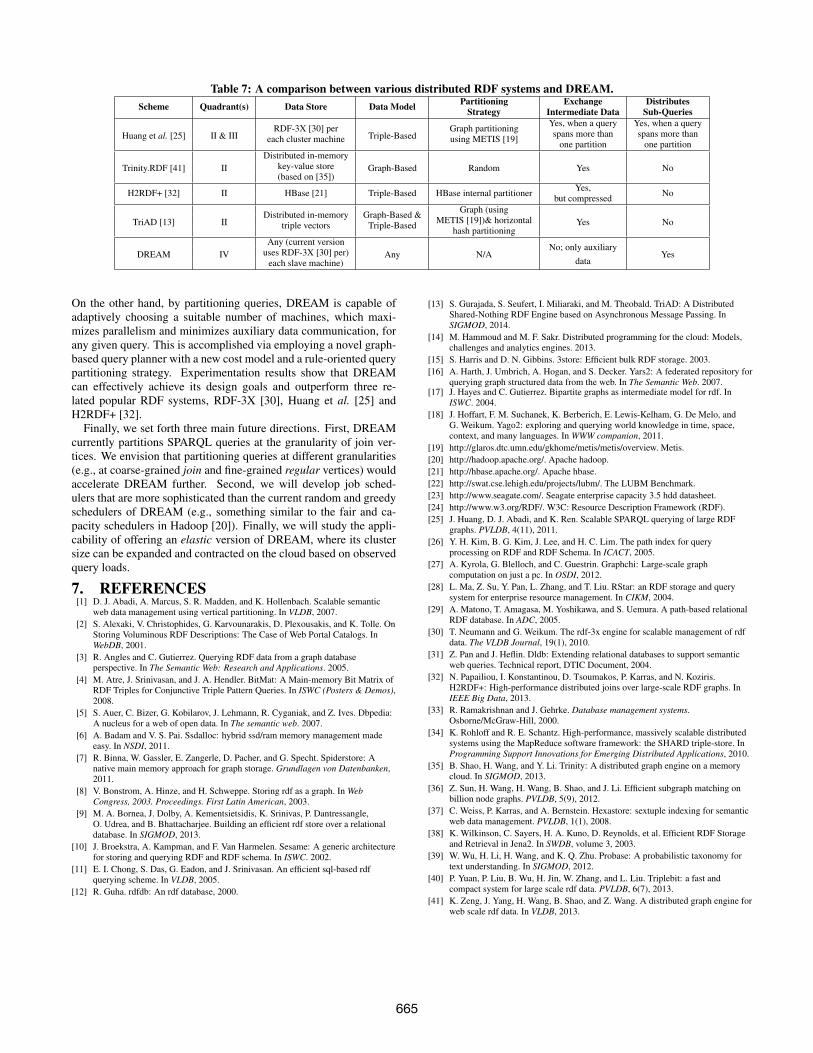
Table 7: A comparison between various distributed RDF systems and DREAM.Scheme Quadrant(s) Data Store Data Model Partitioning Exchange Distributes
Strategy Intermediate Data Sub-Queries
Huang et al. [25] II & IIIRDF-3X [30] per
Triple-BasedGraph partitioning Yes, when a query Yes, when a query
each cluster machine using METIS [19] spans more than spans more thanone partition one partition
Trinity.RDF [41] IIDistributed in-memory
Graph-Based Random Yes Nokey-value store(based on [35])
H2RDF+ [32] II HBase [21] Triple-Based HBase internal partitioner Yes, Nobut compressed
TriAD [13] IIDistributed in-memory Graph-Based & Graph (using
Yes Notriple vectors Triple-Based METIS [19])& horizontalhash partitioning
DREAM IVAny (current version
Any N/ANo; only auxiliary
Yesuses RDF-3X [30] per)each slave machine) data
On the other hand, by partitioning queries, DREAM is capable ofadaptively choosing a suitable number of machines, which maxi-mizes parallelism and minimizes auxiliary data communication, forany given query. This is accomplished via employing a novel graph-based query planner with a new cost model and a rule-oriented querypartitioning strategy. Experimentation results show that DREAMcan effectively achieve its design goals and outperform three re-lated popular RDF systems, RDF-3X [30], Huang et al. [25] andH2RDF+ [32].
Finally, we set forth three main future directions. First, DREAMcurrently partitions SPARQL queries at the granularity of join ver-tices. We envision that partitioning queries at different granularities(e.g., at coarse-grained join and fine-grained regular vertices) wouldaccelerate DREAM further. Second, we will develop job sched-ulers that are more sophisticated than the current random and greedyschedulers of DREAM (e.g., something similar to the fair and ca-pacity schedulers in Hadoop [20]). Finally, we will study the appli-cability of offering an elastic version of DREAM, where its clustersize can be expanded and contracted on the cloud based on observedquery loads.
7. REFERENCES[1] D. J. Abadi, A. Marcus, S. R. Madden, and K. Hollenbach. Scalable semantic
web data management using vertical partitioning. In VLDB, 2007.[2] S. Alexaki, V. Christophides, G. Karvounarakis, D. Plexousakis, and K. Tolle. On
Storing Voluminous RDF Descriptions: The Case of Web Portal Catalogs. InWebDB, 2001.
[3] R. Angles and C. Gutierrez. Querying RDF data from a graph databaseperspective. In The Semantic Web: Research and Applications. 2005.
[4] M. Atre, J. Srinivasan, and J. A. Hendler. BitMat: A Main-memory Bit Matrix ofRDF Triples for Conjunctive Triple Pattern Queries. In ISWC (Posters & Demos),2008.
[5] S. Auer, C. Bizer, G. Kobilarov, J. Lehmann, R. Cyganiak, and Z. Ives. Dbpedia:A nucleus for a web of open data. In The semantic web. 2007.
[6] A. Badam and V. S. Pai. Ssdalloc: hybrid ssd/ram memory management madeeasy. In NSDI, 2011.
[7] R. Binna, W. Gassler, E. Zangerle, D. Pacher, and G. Specht. Spiderstore: Anative main memory approach for graph storage. Grundlagen von Datenbanken,2011.
[8] V. Bonstrom, A. Hinze, and H. Schweppe. Storing rdf as a graph. In WebCongress, 2003. Proceedings. First Latin American, 2003.
[9] M. A. Bornea, J. Dolby, A. Kementsietsidis, K. Srinivas, P. Dantressangle,O. Udrea, and B. Bhattacharjee. Building an efficient rdf store over a relationaldatabase. In SIGMOD, 2013.
[10] J. Broekstra, A. Kampman, and F. Van Harmelen. Sesame: A generic architecturefor storing and querying RDF and RDF schema. In ISWC. 2002.
[11] E. I. Chong, S. Das, G. Eadon, and J. Srinivasan. An efficient sql-based rdfquerying scheme. In VLDB, 2005.
[12] R. Guha. rdfdb: An rdf database, 2000.
[13] S. Gurajada, S. Seufert, I. Miliaraki, and M. Theobald. TriAD: A DistributedShared-Nothing RDF Engine based on Asynchronous Message Passing. InSIGMOD, 2014.
[14] M. Hammoud and M. F. Sakr. Distributed programming for the cloud: Models,challenges and analytics engines. 2013.
[15] S. Harris and D. N. Gibbins. 3store: Efficient bulk RDF storage. 2003.[16] A. Harth, J. Umbrich, A. Hogan, and S. Decker. Yars2: A federated repository for
querying graph structured data from the web. In The Semantic Web. 2007.[17] J. Hayes and C. Gutierrez. Bipartite graphs as intermediate model for rdf. In
ISWC. 2004.[18] J. Hoffart, F. M. Suchanek, K. Berberich, E. Lewis-Kelham, G. De Melo, and
G. Weikum. Yago2: exploring and querying world knowledge in time, space,context, and many languages. In WWW companion, 2011.
[19] http://glaros.dtc.umn.edu/gkhome/metis/metis/overview. Metis.[20] http://hadoop.apache.org/. Apache hadoop.[21] http://hbase.apache.org/. Apache hbase.[22] http://swat.cse.lehigh.edu/projects/lubm/. The LUBM Benchmark.[23] http://www.seagate.com/. Seagate enterprise capacity 3.5 hdd datasheet.[24] http://www.w3.org/RDF/. W3C: Resource Description Framework (RDF).[25] J. Huang, D. J. Abadi, and K. Ren. Scalable SPARQL querying of large RDF
graphs. PVLDB, 4(11), 2011.[26] Y. H. Kim, B. G. Kim, J. Lee, and H. C. Lim. The path index for query
processing on RDF and RDF Schema. In ICACT, 2005.[27] A. Kyrola, G. Blelloch, and C. Guestrin. Graphchi: Large-scale graph
computation on just a pc. In OSDI, 2012.[28] L. Ma, Z. Su, Y. Pan, L. Zhang, and T. Liu. RStar: an RDF storage and query
system for enterprise resource management. In CIKM, 2004.[29] A. Matono, T. Amagasa, M. Yoshikawa, and S. Uemura. A path-based relational
RDF database. In ADC, 2005.[30] T. Neumann and G. Weikum. The rdf-3x engine for scalable management of rdf
data. The VLDB Journal, 19(1), 2010.[31] Z. Pan and J. Heflin. Dldb: Extending relational databases to support semantic
web queries. Technical report, DTIC Document, 2004.[32] N. Papailiou, I. Konstantinou, D. Tsoumakos, P. Karras, and N. Koziris.
H2RDF+: High-performance distributed joins over large-scale RDF graphs. InIEEE Big Data, 2013.
[33] R. Ramakrishnan and J. Gehrke. Database management systems.Osborne/McGraw-Hill, 2000.
[34] K. Rohloff and R. E. Schantz. High-performance, massively scalable distributedsystems using the MapReduce software framework: the SHARD triple-store. InProgramming Support Innovations for Emerging Distributed Applications, 2010.
[35] B. Shao, H. Wang, and Y. Li. Trinity: A distributed graph engine on a memorycloud. In SIGMOD, 2013.
[36] Z. Sun, H. Wang, H. Wang, B. Shao, and J. Li. Efficient subgraph matching onbillion node graphs. PVLDB, 5(9), 2012.
[37] C. Weiss, P. Karras, and A. Bernstein. Hexastore: sextuple indexing for semanticweb data management. PVLDB, 1(1), 2008.
[38] K. Wilkinson, C. Sayers, H. A. Kuno, D. Reynolds, et al. Efficient RDF Storageand Retrieval in Jena2. In SWDB, volume 3, 2003.
[39] W. Wu, H. Li, H. Wang, and K. Q. Zhu. Probase: A probabilistic taxonomy fortext understanding. In SIGMOD, 2012.
[40] P. Yuan, P. Liu, B. Wu, H. Jin, W. Zhang, and L. Liu. Triplebit: a fast andcompact system for large scale rdf data. PVLDB, 6(7), 2013.
[41] K. Zeng, J. Yang, H. Wang, B. Shao, and Z. Wang. A distributed graph engine forweb scale rdf data. In VLDB, 2013.
665