,I

I

I ~.·.·. I

DRD DISCUSSION PAPER

Report Noo ORD256

GOVERNMENT DEFICITS 1 PRIVATE INVESTMENT AND THE CURRENT ACCOUNT: AN INTERTEMPORAL DISEQUILIBRIUM ANALYSIS

by

Sweder van Wijnbergen

March 1987

Development Research Department Economics and Research Staff

World Bank

The TrJorld Bank does not accept responsibility for the views expressed herein \·Jhich are those of the author(s) and should not be attributed to the World Bank to its affiliated organizationsG The findings~ interpretations, and conclusions are the results of research supported by the Bank; they do not necessarily represent official policy of the Banko The designations employed

1 the presentation of material:il and any maps used in this document are solely for the convenience of the reader and do not imply the expression of any opinion whatsoever on the part of the World Bank or its affiliates concerning the status of any territory, city, area~ or of its authorities?

concern delimita ons of its boundaries, or national affiliationo

Pub

lic D

iscl

osur

e A

utho

rized

Pub

lic D

iscl

osur

e A

utho

rized

Pub

lic D

iscl

osur

e A

utho

rized

Pub

lic D

iscl

osur

e A

utho

rized

Pub

lic D

iscl

osur

e A

utho

rized

Pub

lic D

iscl

osur

e A

utho

rized

Pub

lic D

iscl

osur

e A

utho

rized

Pub

lic D

iscl

osur

e A

utho

rized

GOVERNMENT DEFICITS, PRIVATE INVESTMENT AND THE CURRENT ACCOUNT: AN INTERTEMPORr~~ DISEQUILIBRIUM ANALYSIS

Sweder van Wijnbergen World Bank

CEPR and NBER

First Draft June 1984 January 1987

Revised March 1987

I am indebted to John Cuddington for helpful comments. The World Bank does not accept responsibility for the views expressed herein which are those of the author.

SUMMARY

We use a model with full intertemporal optimization and Fischer-Gray

type short run real wage rigidities to demonstrate the effects of deficit

spending in different employment regimes. We allow for upward price

flexibility,.although prices, once set at the beginning of the period, will be

rigid downward until the beginning of the next period. We show that under

Keynesian unemployment (conditional on a plausible assumption about public and

private sector discount rates) deficit spending reduces unemployment, impro,res

the future terms of trade and therefore leads to an increase in private

investment (crowding in) and to a deterioration of the Current Account.

Under classical unemployment, goods markets clear but unemployment

persists because of contract based real wage rigidity. Fiscal expansion then

goes partly into prices (terms of trade improvement) and only partly into

quantities. The latter occurs to the extent that contract based real

consumption wage rigidity, coupled with a terms of trade improvement, allows a

lower real product wage. A temporary increase in government expenditure in

classical unemployment leads to a bigger terms of trade improvement today than

tomorrow, so both income and substitution effects lead to a current account

improvement. The cost of capital increases more than the value of future

o?tput and investment falls. This also improves the first period current

account. The direct impact of increased first period government expenditure

may offset these surprising positive effects on the first period current

account.

Finally we show that, the more open the economy is, the larger is

the output response and the smaller the price response to a fiscal expansion

in the presence of classical unemployment. This contrasts with the Keynesian

unemployment regime, where a higher import component in expenditure leads to

more dissipation of effective demand and smaller output effects.

II

III.

IV.

v.

Table of Contents

Introduction

An Intertemporal Contract-Based Disequilibrium ~.fodel

Fiscal Policy Under Keynesian Unemployment

Fiscal Policy Under Classical Unemployment

Conclusions

Appendix

Page No

1

3

18

24

30

35

1

I. Introduction

The emergence of substantial government deficits in the late

seventies and early eighties has brought government deficits and their effects

on the economy back to the foreground of policy debate. Large deficits in the

US played a part in the remarkably fast recovery in 1983 and 1984, but, so

many observers claim, at the cost of high real interest rates and external

deficits on current account. Investment has recovered strongly however, high

real interest rates notwithstanding. In Western Europe large deficits have

not prevented increasing unemployment, while private investment has remained

extremely weak. An extreme example is Holland where large government deficits

have gone together with ever increasing unemployment, collapsing private

investment and, surprisingly enough, substantial current account surpluses.

The existing literature does not give us too much guidance in

explaining these developments. Two strands can be distinguished. The first

goes back to Keynes (1936), Hicks (1939) and Haavelmo (1945). The focus here

is exclusively on short-run aggregate demand effects; a traditional set up of

static consumption functions and demand-driven supply is used. Disequilibrium

in labor and goods markets is not explicitly incorporated, while the·

intertemporal aspects (e.g. less taxes today means more taxes tomorrow) are

typically ignored.

The other strand in the literature focuses almost exclusively on

these intertemporal aspects. One of the best known examples of this part of

the literature is Barra (1974). In contrast to the earlier literature, these

authors base private behavior on explicit intertemporal optimization. That

allows a satisfactory analysis of changes in the intertemporal pattern of

taxes; an ambitious open economy extension of this literature is Frenkel and

Razin (1985a). However, their use of full employment, market clearing models

2

precludes a meaningful discussion of the stabilization aspects of fiscal

policy.

In this paper we will attempt to bring the two strands together. We

analyze fiscal policy in the context of a model with intertemporal optimiza­

tion underlying private behavior. But we also explicitly incorporate the

possibility of (short-run) labor and goods market disequilibrium caused by

Fischer (1977)-Gray (1978) type contract-based real wage rigidities and

within-period downward price inflexibility. Prices are however assumed to be

flexible upward, in a departure from the standard disequilibrium literature.

There is both theoretical and empirical support for such an asymmetry. We

discuss this further in Section II. In another departure from the standard

disequilibrium literature, but in line with modern contract theory, we

incorporate temporary real consumption wage rigidity, rather than permanent,

nominal wage rigidity.

This potentia1 for labor and goods market disequilibrium allows us

to address stabilization aspects of fiscal policy (impact on aggregate output

and employment). Cuddington and Vinals (1986a,b) also incorporate temporary

disequilibrium in an intertemporal optimization model in their discussion of

fiscal policy. They focus on monetary aspects and moreover maintain complete

within-period nominal-wage-price rigidity, as opposed to our assumptions of

asymmetric price adjustment (flexible upwards but rigid downward) and contract

based real consumption-wage rigidity. Moreover, they ignore investment and

have to rely on very restrictive functional forms, thereby eliminating many of

the intertemporal relative price effects that play an important role in our

analysis. Other disequilibrium models incorporating rational optimizing

saving and investment behavior can be found in Bruno (1982), Neary and

Stiglitz (1983) and van Wijnbergen (1985).

3

In Section II the basic model is presented. We use a two-period

model where wages and prices are set at the beginning of each period using all

available information. This is done in auch a way that all markets will be in

equilibrium if no unanticipated events occur after the contracts have been

concluded. If such events do occur, there may be disequilibrium in labor and

goods markets. The implications of that are analyzed in the tradition of

Barro-Grossman (1976), Benassy (1975) and Malinvaud (1977), while maintaining

an explicit intertemporal optimization framework and allowing for upward price

flexibility, contrary to much of the existing disequilibrium literature.

Fiscal policy effects under Keynesian unemployment are analyzed in Section

III, while Section IV looks at the case of classical unetn ... oyment. Section V

concludes.

II. An Intertemporal, Contract-Based Disequilibrium Model

A. Consider a two-period, two-commodity world. Period one corresponds

to the. "short run". In this period, the capital stock cannot be adjusted and

wage-price rigidities may exist. All shocks taking place in this period are

unanticipated. In the second period, the "long run", wages, prices and the

capital stock can adjust. An artificial but innocuous consequence of the two­

period structure is that no investment takes place in the second period~

Another implication of the two-period structure is that all debts carried over

from period one need to be paid off in period two.

The economy specializes completely in the production of good 1 while

foreigners specialize in the 'production of good 2. Firms use the beginning of

period capital stock and labor as factors of production, and determine output

based on the size of the capital stock and the level of the real product

wage. This process can be described by using a revenue function (a good

4

exposition of this and other duality tools can be found in Dixit and Norman

(1980)):

R = R(P K,L) (1)

= P X(K,L)

where P is the price of home goods in period 1. Capital letters indicate

first period variables, and lower case symbols second-period variables.

Foreign goods are chosen as numeraire, so we can interpret P and p as the

first and second period terms of trade. Labor demand is given by the

requirement that the marginal value product equals the wage:

Inverting (2) yields a labor demand function L = L(W/P,K) • If we insert that

back into (1) we get:

R = P X(K,L(W/P))

= R(P,W/P)

with output supply equal to

aR X=-= R aP P

= X(K,L(W/P))

(3)

(4)

5

We assume full employment in the second period (the "long run"), for

reasons explained in the beginning of section II.B. As a consequence, second

period output x depends on the second period capital stock only

and

r = r(p,k)

= p x(k)

X = ar ap

(5)

(6)

We ignore depreciation, so k = K + I where I is first period investment.

Investment is determined by value maximizing firms, equalizing the discounted

value of future marginal revenue to the production cost of capital:

ax op ak (K + I) = P (7a}

We assume for simplicity that investment only requires domestic goods as

input. * * o is the discount factor 1 I (1 + p ) with p the world rate of

interest. We assume that the economy is too small to influence the world

* interest rate p •

Equation {7a) yields an investment demand function:

(7b)

6

Equation (7b) also incorporates our assumption of perfect foresight.

We make the same assumption for consumer behavior, to which we turn

now. We make no distinction between consumption patterns of wage earners and

profit recipients. However, we assume that profits are paid out in the period

in which they are earned, contrary to Malinvaud (1977) or Neary (1980). An

expenditure function describes consumer behavior. The expenditure function

gives the minimum discounted value of expenditure needed to reach utility

level U given prices today and tomorrow (again see Dixit and Norman (1980) for

an exposition of expenditure functions):

E = E(IT(P,l), 6n(p,l), U) (8)

where n and n are unit expenditure functions and the exact aggregate price

indices corresponding to the utility structure U. 1/ By the properties of

expenditure functicns we know that domestic consumer demand for home goods, CD

(cD for the second period), equals the derivative of E with respect to the

corresponding price:

(9)

Also IT and n are aggregate price indices, so we can define real expenditure in

each period:

1/ We assume U to be Weakly Identically Homothetically Separable, which allows us to write E as a function of U and the within-period unit expenditure functions nand~ • ·see Razin and Svensson (1983) and van Wijnbergen (1984) for a detailed discussion.

7

(10)

n and n are unit expenditure functions, so np = c0/A and np = c0/a •

Furthermore we can derive similar expressions for foreigners, for whom we will

use starred variables * * * (E , c0

, A etc.) •

Expenditure needs to satisfy the private sector intertemporal budget

constraint:

* * * R + or - PI - T = E, R + or = E (11)

Government and investment in the foreign country are ignored. T equals the

discounted value of ~~rrent and future taxes: T = T + ot with obvious

definitions of T and t. Under the assumption of identical government and

private discount rates, T = P G + opg via the government budget

constraint. (More on this in Section II.E).

First period goods market equilibrium requires:

(12a)

* = Ep + Ep + I(op/P) + G

where G 1s first period government expenditure. Similarly, for period 2:

* r = E + E + g • (12b) p p p

8

(12a, b) embed the assumption that both government and investment expenditure

fall entirely on domestic goods.

We assume a fixed labor supply L, so the labor market equilibrium

condition is given by:

L = L(W/P) (13)

Equations (8) and (11) yield private welfare at home, U, and abroad,

* U , as a function of P, p, T and t:

* * U = U(P, p,T,t), U = U (P, p) {14a)

or, in differentiated form and using (12a,b) to substitute out expressions

like rp- Ep- I- g etc.:

and

* * Ep dP + Ep 6dp - dT - 6dt =

* * = E dU u

E dU u

(14b)

(14c)

(14b,c) are evaluated around G = g = 0 to avoid irrelevant valuation effects

on government expenditure. (11a, b), (12) and (14) constitute an equilibrium

version of the model, with variables P, p,. W/P, U and u*. We will first give

a diagrammatic representation of this equilibrium version, because that will

facilitat~ the introduction of the consequences of first period

disequilibrium.

9

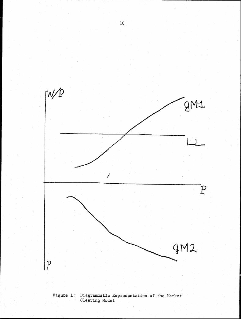
Inserting (14) in (12a) to substitute out U and u* gives us a locus

describing goods market equilibrium in period 1, represented by GM1 in fig. 1:

d(W/P) dP

GM1

2 I: -I'op/P pp

X 1 1

L (15)

* * * with I:pp = Epp + Epp + (CDE - c0E) Ep' the world substitution matrix plus

income effects of an increase in P. I:PP < 0 for normal goods. CDE is

-1 * ("our") marginal propensity to spend on our first period goods, EPUEU • CDE

is the foreign marginal propensity to spend on our ffrst period goods,

* *-1 EPU EU • GM1 is upward sloping: a higher (relative) price of our goods

reduces world demand for our goods, leading to excess supply; a higher real

product wage however will reduce aggregate supply {cf. fig. 1).

Labor market equilibrium is represented by (13), a horizontal line

in the W/P - P plane:

d W/P I dP LL = O (16)

Since labor is the only variable factor in this model, there is only one

market clearing real product wage.

The second period goods market equilibrium locus GM2 slopes upward

(cf. fig. 1 and keep in mind that p increases from 0 downwards):

~ I = dP GM2

(I: p + r k I' op/P2) p p > 0

(I: - r I 1 o/P) PP pk

(17)

where I:pP and I: are the relevant elements of the world substitution matrix pp

(I:pP * * etc); plus income effects = EpP + EpP + (cDE - cDE)Ep I:pP > 0 and I: < 0 pp

* . ) with sufficient symmetry. (CDE not too much larger than CDE

p

10

I

Figure 1: Diagrannnatic Representation of the Harket Clearing Model

p

11

Two channels link p and P via the second period goods market. The

first runs through op/P • For given p, a higher P raises the production

cost of capital which will lead to lower investment. That in turn reduces

aggregate supply in period two, leading to upward pressure on p. The second

channel also leads to a positive relation, through substitution effects in

consumption. Higher prices today for given p will decrease the consumption

discount factor on(p,l)/TI(P,l) = 1/(l+CRI) • CRI is the consumption rate of

interest (cf. Little and Mirrees (1974)). This will lead to a shift of

expenditure towards the future because of pure substitution effects, some of

which will fall on period 2 home goods. This also puts upward pressure on

their relative price p, like the effect via the first channel, so there is an

unambiguously positive link between p and P along GM2 (cf. fig. 1).

Before we intr9duce disequilibrium, one final point: the diagram in

Fig. 1 involves a fudge, necessary to allow diagrammatic representation. The

same channels linking p and P via period two goods market clearing also work

backwards: future prices do influence first period goods markets, via the

value of capital in period 2 (and so via first period investment), and via the

impact of the CRI on private savings. This of course implies that we cannot

really represent GMl in W/P -P space. The algebraic derivation of all results

incorporates this extra link, but we will ignore it in the diagrammatic

representation. !/ It is left to the interested reader to demonstrate than an

increase in p shifts GMl to the right.

!1 All algebraic derivations are spelled out in detail in. the mathematical appendix.

12

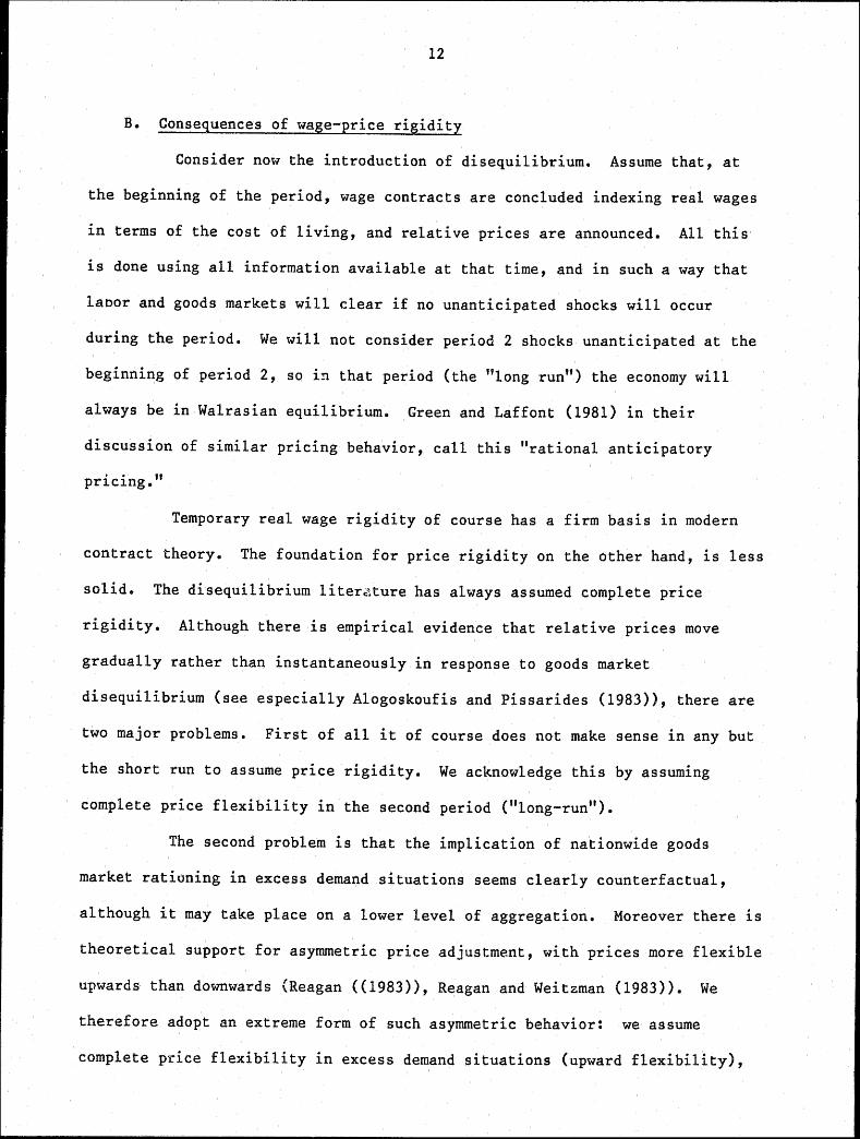
B. Consequences of wage-price rigidity

Consider now the introduction of disequilibrium. Assume that, at

the beginning of the period, wage contracts are concluded indexing real wages

in terms of the cost of living, and relative prices are announced. All this

is done using all information available at that time, and in such a way that

laoor and goods markets will clear if no unanticipated shocks will occur

during the period. We will not consider period 2 shocks unanticipated at the

beginning of period 2, so in that period (the "long run") the economy will

always be in Walrasian equilibrium. Green and Laffont (1981) in their

discussion of similar pricing behavior, call this "rational anticipatory

pricing."

Temporary real wage rigidity of course has a firm basis in modern

contract theory. The foundation for price rigidity on the other hand, is less

solid. The disequilibrium litereture has always assumed complete price

rigidity. Although there is empirical evidence that relative prices move

gradually rather than instantaneously in response to goods market

disequilibrium (see especially Alogoskoufis and Pissarides (1983)), there are

two major problems. First of all it of course does not make sense in any but

the short run to assume price rigidity. We acknowledge this by assuming

complete price flexibility in the second period ("long-run").

The second problem is that the implication of nationwide goods

market rationing in excess demand situations seems clearly counterfactual,

although it may take place on a lower level of aggregation. Moreover there is

theoretical support for asymmetric price adjustment, with prices more flexible

upwards than downwards (Reagan ((1983)), Reagan and Weitzman (1983)). We

therefore adopt an extreme form of such asymmetric behavior: we assume

complete price flexibility in excess demand situations (upward flexibility),

13

but within-period downward rigidity when unanticipated shocks cause excess

supply of goods.

Some modifications to the model are necessary because of potential

disequilibrium and the associated spillover effects. The expression for goods

market equilibrium under excess supply of labor changes, although firms are

not constrained in this situation. But consumers' intertemporal budget

constraint is affected because now employment and therefore income is variable

and will depend on the real product wage. Substituting out U via the modified

budget constraint gives:

aW/P = aP GM1

Epp-I'op/P2

(1-CDEP)X1L' > 0 (18)

Compsrison of (18) with (15} shows that this segment of GM1 will

still be upward sloping, and in fact will be steeper than in the equilibrium

version, because of the term - CDEX1

L' in the denominator. This is because

higher wages will now not only cut aggregate supply, but also demand for home

goods through their negative impact on employment and therefore total

income. This means that a smaller price increase is needed to rebalance goods

markets after a given increase in real product wages W/P: GM1 is steeper

(cf. fig. 2).

The loci describing goods market equilibrium under excess demand for

labor, and labor market equilibrium under excess supply of goods, collapse

into one locus in this type of model without inventories and with complete

specialization of production. This eliminates the so-called "under-

consumptionist" regime.

In the area above LL and to the left of GMl, pri~es and wages are

such that labor is in excess supply and domestic goods in excess demand.

14

W/1?

(I<)

f

Figure 2: First Period Disequilibrium Regions and Second Period Goods Market Clearing Locus

15

However, because of our assumption of upward price flexibility, the economy

will never be in that region: prices will increase until the economy is on

the GMl locus, with goods markets in equilibrium, but real wages too high for

labor market equilibrium.

Accordingly, one unemployment regime is the K-region to the right of

GMl, with Keynesian unemployment: here output is demand-determim~d because

prices are set too high for all the supply to be absorbed. The second regime

is along the GMl locus from the Walrasian equilibrium point W upwards, with

the goods market in equilibrium but real wages too high for labor market

clearing. We will call this regime classical unemployment, although it is

different from what is commonly called classical unemployment in the

disequilibrium literature: our "c region" is not characterized by goods

market rationing. 1/

The GM2 locus will now change and will depend on the regime

prevailing in period 1. However, it is still sloped as in fig. 1 in all three

cases. So we can use the diagram in fig. 2 as long as no regime switches are

considered"

C. The Keynesian Unemployment Regime.

The behavioral equations of course change discontinuously across

regimes. Consider first the K-region. First period output in that region is

demand determined:

(19)

1/ The C-region as defined here corresponds to the boundary between the Keynesian and classical regions in more conventional disequilibrium models.

16

where Rp > X • Second period goods market equilibrium is similar to 12b:

r (K + I) = p

* E + E + g p p

(20)

but the domestic private intertemporal budget constraint is different:

PX + or - PI - T = E (21)

where PX replaces R {note that R > PX in this regime!). The foreign budget

constraint remains unchanged.

D. The Classical Unemployment Regime.

Under classical unemployment, first period output is supply

determined and prices (P) will adjust until goods markets clear. Accordingly

the following goods. market clearing condition holds:

Second period goods market equilibrium, as before, is represented by:

r (p,K + I) p * = E + E + g

p p

(22)

(23)

The difference from the equilibrium model of Section 2.2 lies in the

labor market: wages are fixed in terms of the cost of living, at a level that

would have led to labor market clearing if no unanticipated shock had occurred

17

after the conclusion of wage contracts. We have an exact measure of the first

period cost of living via our unit expenditure function IT , so:

w/rr = w (24)

Finally the domestic private intertemporal budget constraint:

-R(P,W/P) + or(p,K+I) - T - P I = E (25)

Employment in this regime is of course demand determined: by

inverting equation (3) we get:

L = L(W/P) (26)

Note that prices are flexible upwards while there is real consumption wage

rigidity. Accordingly the real product wage W/P is not rigid.

The model applying to the Repressed Inflation regime is left to the

interested reader to explore since we will not be concerned with that regime

in this paper.

E. The Government Budget Constraint.

Before turning to the analysis of fiscal policy, a discussion of the

government budget constraint is in order. The benchmark case involves equal

discount rates for public and private sector. This implies

PG + opg = T+ot(= T) (27)

18

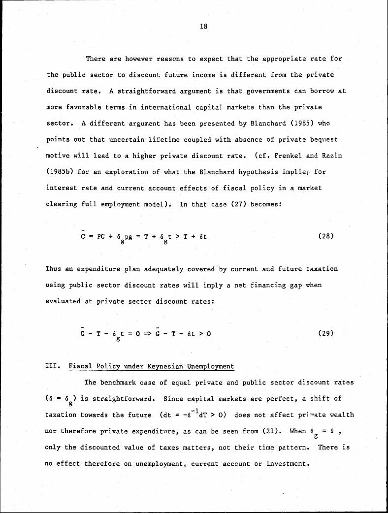
There are however reasons to expect that the appropriate rate for

the public sector to discount future income is different from the private

discount rate. A straightforward argument is that governments can borrow at

more favorable terms in international capital markets than the private

sector. A different argument has been presented by Blanchard (1985) who

points out that uncertain lifetime coupled with absence of private beqnest

motive will lead to a higher private discount rate. (cf. Frenkel and Razin

(1985b) for an exploration of what the Blanchard hypothesis implier for

interest rate and current account effects of fiscal policy in a market

clearing full employment model). In that case (27) becomes:

G = PG + 5 pg = T + o t > T + ot g g

(28)

Thus an expenditure plan adequately covered by current and future taxation

using public sector discount rates will imply a net financing gap when

evaluated at private sector discount rates:

G - T - o t = 0 => G - T - ot > 0 g

III. Fiscal Policy under Keynesian Unemployment

(29)

The benchmark case of equal private and public sector discount rates

(o = o ) is straightforward. Since capital markets are perfect, a shift of g

taxation towards the future (dt = -o-1dT > 0) does not affect pri~~ate wealth

nor therefore private expenditure, as can be seen from (21). When o = o , g

only the discounted value of taxes matters, not their time pattern. There is

no effect therefore on unemployment, current account or investment.

19

Similar results obtain for a deficit financed increase in gov~rnment

expenditure; we can see from (19) that dX/dG = 1 as a first round effect; but

since dT ~ PdX , nothing happens to private wealth and expenditure and no

multiplier effects occur. Accordingly, private investment and the current

account do not change either. Clearly Keynesian disequilibrium and wage-price

rigidities are not sufficient for a multiplier larger than one.

Private and social discount rate differences will change all this,

however. The discount factor wedge implies that an increase in government

expenditure fina~~ced by taxes tomorrow (i.e. a bond issue today) will not be

considered neutral by the private sector; the government budget constraint

implies that

so

PdG = o .dt g

PdG - dT = PdG - odt

= {o - o}dt > o g

(30)

Total differentiation of the Keynesian system (21)-(23) yields:

dU A (o -o) > o Eu dG = M g (31)

g

A, A > 0 ; Analytical expressions for A and !J. are listed in the Appendix.

(31) establishes that a temporary bond financed expansion in

government expenditure will unambiguously increase private welfare in

Keynesian unemployment if 0 > 0 • g

It is straightforward to show that a

current-tax financed temporary fiscal expanr.ion would not do that.

20

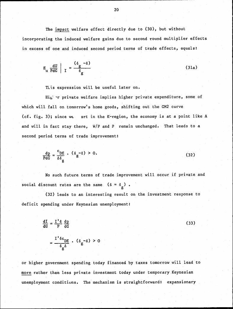
The impact ~elfare effect directly due to (30), but without

incorporating the induced welfare g~ins due to second round multiplier effects

in excess of one and induced second period terms of trade effects, equals:

(o -o)

I g

I = ----:o"---g

(3la)

Ti.is expression will be useful later on.

Hig': 'r private welfare implies higher private expenditure, some of

which will fall on tomorrow's home goods, shifting out the GM2 curve

(cf. fig. 3); since w~ art in the K-region, the economy is at a point like A

and will in fact stay there; W/P and P remain unchangeds That leads to a

second period terms of trade improvement:

c ~ _ DE • (o -o) > o. PdG - M g (32)

g

No such future terms of trade improvement will occur if private and

social discount rates are the same (o = o ) • g

(32) leads to an interesting result on the investment response to

deficit spending under Keynesian unemployment:

di = I'o ~ dG P dG

= I'ocDE • (o -o) > o 0 h. g g

(33)

or higher government spending today financed by taxes tomorrow will lead to

~ rather than less private investment today under temporary Keynesian

unemployment conditions. The mechanism is straightforward: expansionary

21

W/J?. /

LL /~A / I

/ I --.--- ' ' '- I

' I ,, ,, I I I

--- .-. .......... ..,.__ ..,.-........___ ·-~~-- -----

............... .............._

~ I _....._. _________ .__ ............._ I -----------~

Figure 3:

~

Effects of a Bond Financed Increase in G when 8 > 8 g

22

fiscal policy raises welfare (if o > a} g and therefore first and second

period expenditure. This pushes up the future terms of trade p, which in turn

increases the value of the marginal product of capital in period 2: the goods

produced with that capital now have a higher value. Tobin's "q" goes up and

so does private investment. This result is the opposite of the crowding out

hypothesis: in fact under temporary Keynesian unemployment there will be

crowding in as private investment responds positively to the future terms of

trade improvement caused by the fiscal expansion. !/

Moreover part of the increase in private expenditure will fall on

today's goods, the equivalent of second and higher rounds of induced spending

familiar from standard macro-economic textbooks, so now we do get a multiplier

in excess of one:

(r I'o/P- L )Pc dX _ pk :e£_ DE dG- 1 + -----11o-- -- · (ag-o)

g (34)

(A)

+ (I: + I'o/P) Pc Pp DE • (o -o)

g 11o g

(B)

>dG

!/ A referee points out that imperfect capital mobility or assuming that the domestic economy is large enough to affect the world rate of interest would lead to an increase in real interest rates after a fiscal expansion, which could reverse this result.

23

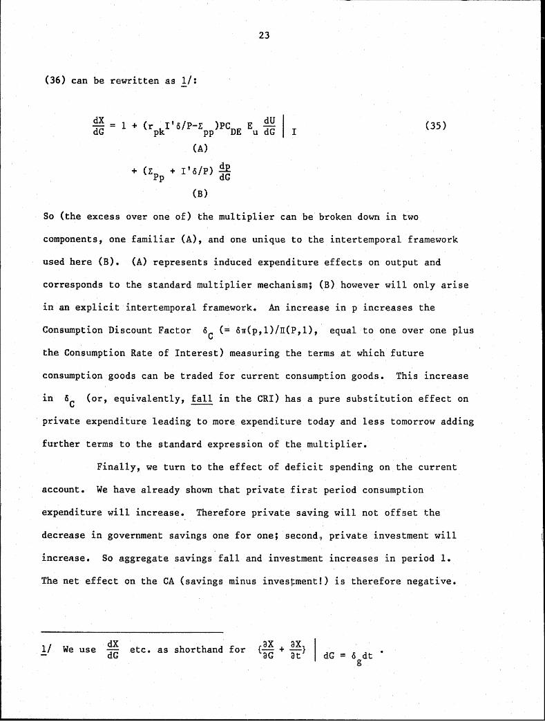
{36) can be rewritten as 1/:

~ = 1 + (rpki'5/P-Epp}PCDE Eu ~g I 1

{A)

+ (E + I'o/P) ~ Pp dG

(B)

So (the excess over one of) the multiplier can be broken down in two

(35)

components, one familiar (A), and one unique to the intertemporal framework

used here (B). (A) represents induced expenditure effects on output and

corresponds to the standard multiplier mechanism; (B) however will only arise

in an explicit intertemporal framework. An increase in p increases the

Consumption Discount Factor oC (= on(p,l)/IT(P,l), equal to one over one plus

the Consumption Rate of Interest) measuring the terms at which future

consumption goods can be traded for current consumption goods. This increase

in oC (or, equivalently, fall in the CRI) has a pure substitution effect on

private expenditure leading to more expenditure today and less tomorrow adding

further terms to the standard expression of the multiplier.

Finally, we turn to the effect of deficit spending on the current

account. We have already shown that private first period consumption

expenditure will increase. Therefore private saving will not offset the

decrease in government savings one for one; second.~ private investment will

increase. So aggregate savings fall and investment increases in period 1.

The net effect on theCA (savings minus inves~ment!) is therefore negative.

1/ We use dX dG etc. as shorthand for {ax + ax}

aG at 0 dt g

24

A permanent increase in government expenditure (PdG = opdg > 0)

would add further upward pressure on tomorrow's terms of trade, and so on

investment. It would also lead to more private consumption via income effects

and substitution effects through the CRI in period one. This would magnify

the negative impact on the first period current account deficit. The formal

analysis is straightforward and left to the interested reader.

IV. Fiscal Policy Under Classical Unemployment.

Under Classical unemployment the benchmark case 0 = 0 g

is of more

interest than in the Keynesian case, since increases in first period

expenditure cannot be met at unchanged prices. To avoid excessive taxonomy,

we will in fact only consider the benchmark case.

Increased first period government expenditure on our goods (dG > 0)

is, at given wages and prices, inconsistent with first period goods market

clearing, since in this regime firms are on their aggregate supply curve.

Accordingly the terms of trade will have to improve to accommodate increased

government expenditure, or GMl shifts to the right (fig. 4):

dP dG GMl

W/P = W/P

(36)

However, G goes up after real wage contracts have been concluded at

the beginning of period one. They can be renegotiated at the beginning of the

second period, but during period one the real consumption wage W/IT(P,l) is

fixed. This means that:

25

w;.e

p

' I I I I I I I ICJ ~ .............

............. '"""'-

Figure 4: Effects of a Fiscal Expansion Under Classical Unemployment

26

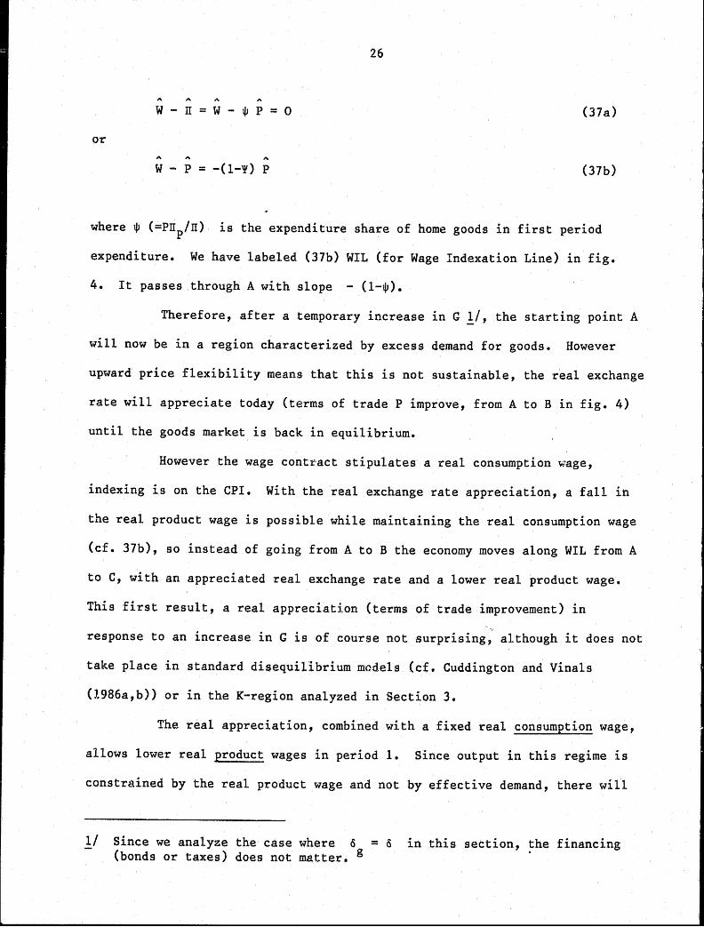
w - rr = w - w P = o (37a)

or

W - P = -(1-Y) P (37b)

where ~ (=Prrp/rr) is the expenditure share of home goods in first period

expenditure. We have labeled (37b) WIL (for Wage Indexation Line) in fig.

4. It passes through A with slope - (1-~).

Therefore, after a temporary increase in G 11, the starting point A

will now be in a region characterized by excess demand for goods. However

upward price flexibility means that this is not sustainable, the real exchange

rate will appreciate today (terms of trade P improve, from A to B in fig. 4)

until the goods market is back in equilibrium.

However the wage cont~act stipulates a real consumption wage,

indexing is on the CPI. With the real exchange rate appreciation, a fall in

the real product wage is possible while maintaining the real consumption wage

(cf. 37b), so instead of going from A to B the economy moves along WIL from A

to C, with an appreciated real exchange rate and a lower real product wage.

This first result, a real appreciation (terms of trade improvement) in

response to an increase in G is of course not surprising, although it does not

take place in standard disequilibrium models (cf. Cuddington and Vinals

(!986a,b)) or in the K-region analyzed in Section 3.

The real appreciation, combined with a fixed real consumption wage,

allows lower real product wages in period 1. Since output in this regime is

constrained by the real product wage and not by effective demand, there will

1/ Since we analyze the case where o = o (bonds or taxes) does not matter. g

in this section, the financing

27

in fact be some increase in output, although less than in the K-region. In

the C-region, the effect of an increase in fiscal exp~nditure goes partly into

prices (dP > 0), partly into quantities. In the K-region it only goes into

quantities.

It is of interest to see what determines how the value increase is

split up over quantities and prices. Clearly the flatter WIL, the more the

effect consists of a real appreciation and the less it consists of a real

product wage cut induced output increase. The slope of WIL, (1-$) , can be

considered a measure of openness of the economya A very flat line implies $

is close to one, imports do not play much of a role and therefore any given

real appreciation buys only a small decrease in the domestic real product

wage. This leads to the interesting result that in the C-region (GMl axis

north of E), more openness means a larger output response and a smaller price

response to fiscal expansion. This contrasts with the K-region where a higher

import component in expenditure leads to more dissipation of effective demand

and smaller output effects.

The effects on the second period terms of trade are ambiguous in the

case of a temporary increase in G. In that case the GM2 locus shifts back to

the zero p-axis (fig. 4), since the impact welfare effect of G on U for given

wages and prices is negative; the government's increased use of first period

resources implies they are not available for the private sector, with a

welfare loss as a result. This spills over into period two, reducing "our"

expenditure (ceteris paribus) and therefore causing an ex ante excess supply

of home goods. Accordingly their relative price will have to fall to maintain

period two goods market equilibrium:

_ip_ PdG GM2

P=P

(38)

28

or GM2 shifts down (compare D and F in Fig. 4). Ec is defined in the PP

appendix.

On the other hand the real appreciation in period one causes

intertemporal substitution effects on consumption, increasing second period

demand for our goods. Moreover, since dP > 0 implies that the production cost

of capital increases, first period investment falls (there is crowding out in

the C-region), reducing the supply of period 2 home goods. The latter effect

is of course dependent on our assumption that only domestic goods are used for

investments. Both factors work toward a real appreciation (a move along GM2

from F to G). The net effect is ambiguous.

It is shown in the appendix that, even if there is a second period

real appreciation dp > 0, it will be smaller than the first period one, so

that the consumption discount factor ~ = 1/(1 + CRI) and the capital c

discount factor oh = op/P decrease unambiguously. In other words, the

Consumption Rate of Interest and the Accounting Rate of Interest go up

unambiguously. This leads to a rather surprising possibility of a positive

current account response to increased first period fiscal expenditure, even

when it is deficit financed (i.e. by bonds rather than taxation).

There are a variety of channels influencing the CA response. The

formal expression, where for convenience we look at CA2 rather than CA1

,

(since CA1 + oCA2 = 0 one can take either one), is:

= d(r-E 1T-pg) 1f

= I,.§_£ (.!!£ - dP) rk p p p

(39)

(A)

+ E II2 o (!!£ - dP) niT o • c p P

29

. (B)

(CJ

(D)

(E)

CIE(CIIE) 1s the marginal propensity to spend in period one (two).

Consider the five effects in turn for a temporary increase in

government expenditure, PdG > 0, pdg = 0. We already saw that in that case

dP > ~ p p •

Channel (A) indicates that such an increase in the cost of capital

in excess of future value of marginal product gains (dP > ~} will lead to a p p

fall in first period 5nvestment. That in turn causes a fall in second period

capital and output and so an improvement in CA1 (decline in CA2).

S · ·1 1 dP dn h · · b · · ff 1m1 ar y, -p > ~ as pos1t1ve pure su st1tut1on e ects,

proportional to Enrr , on first period savings which improves CA1

.(deteriorates CA2). This is captured by channel (B). If spending patterns

here and abroad are similar etc.), terms of trade change induced

income effects will not influence the CA; but if we spend more today and less

tomorrow than foreigners do the higher terms of

trade gain today associated with a temporary increase in fiscal expenditure

will improve CA1 (deteriorate CA2). This is channel c.

Furthermore the first period real appreciation, coupled with real

consumption wage indexation, allows a fall in real product wages and an

30

increase in first period output. This improves CA1 (deteriorates CA2), as

captured by channel D.

Finally, the direct effect of increased fiscal expenditure

deteriorates the CA, but this effect is moderated because it leads to a fall

in welfare which in turn leads to an equal present value drop in private

expenditure. For a temporary increase, consumption smoothing explains why

this private cut only pa~tially offsets the first period direct current

account effects. So this channel (E) leads to a deterioration in CA1 and an

improvement in CA2•

Summing up, (A), (B), and (D) are positive influences on the first

period CA: (C) is positive if the home country is more impatient (saves less)

than the foreign country, while (E) has a negative impact on CA1• A positive

first period CA response to a temporary increase in government expenditure is

therefore a distinct possibility.

V. Conclusion

We use a 2-period model with optimizing private agents, real wage

indexation and downward price rigidity to demonstrate the effects of deficit

spending in different employment regimes. The effects of fiscal policy are

shown to depend crucially on the type of unemployment (Keynesian or Classical}

that prevails.

In a Keynesian unemployment regime, deficit spending increases

output and employment. If a plausible assumption about government and private

discount rates is introduced, we obtain an interesting result on the private

investment response. If private discount ra~es exceed social discount rates,

private consumption expenditure will increase both today and tomorrow in

response to the increase in public expenditure, in spite of full anticipation

31

of the increased future tax liabilities. Increased future consumption

expenditure will lead to a fully anticipated future terms of trade improvement

(the price of home goods in terms of foreign goods goes up). This increases

the value of the marginal product of capital relative to its (first period)

production costs and triggers an increase in private investment in period 1.

That is, deficit spending under Keynesian unemployment will lead to crowding

in rather than crowding out. Similarly, the increase in private consumption

expenditure today coupled with higher government deficits and increased

private investment lead to an unambiguously negative link between deficit

spending and the current account in this unemployment regime.

The effects of fiscal policy are very different when unemployment is

caused by real wages in excess of their market clearing level, leading to low

output and employment because of insufficient profitability. Assuming output

prices are flexible upwards, a temporary increase in government expenditure in

this classical unemployment regime leads to larger terms of trade improvements

today than tomorrow. As a result both iccome and substitution effects lead to

a CA improvement. Investment will decline ("crowding out"), furthe1 improving

the current account. The direct (i.e. for given wages and prices) impact of

increased first-period government expenditure tends to at least partially

offset these surprising positive effects on the CA; the net effect is

ambiguous. It is of interest however to note at least the possibility of a

first period CA improvement in response to a temporary increase in government

expenditure under classical unemployment.

Finally we show tha~ t:1e more open the economy is, t~~-e larger is t:he

output response and the smaller the price response to a fiscal expansion in

the presence of classical unemployment. This contrasts with the Keynesian

32

unemployment regime, where a higher import component in expenditure leads to

more dissipation of effective demand Mnd smaller output effects.

33

REFERENCES

Alogoskoufis, G. and C. Pissarides (1983), "A Test of Price Sluggishness in a simple Rational Expectations Model: Britain 1950-1980", Economic Journal, val. 93, pp. 616-628.

Barra, R. (1974), "Are Government Bonds Net Wealth?", Journal of Political Economy, val. 82, pp. 1095-1117.

Barra, R. and H. Grossman (1976), Money, Employment and Inflation, Cambridge University Press.

Benassy, J. P. (1975), "Neo-Keynesian Disequilibrium Theory in a Monetary Economy," Review of Economic Studies, val. 42, pp. 503-524.

Blanchard, 0, (1985), "Debt, Deficits and Finite Horizons," Journal of Political Economy, vol. 93, pp. 223-247.

Bruno, M. (1982), "Macroeconomic Adjustment under Wage-Price Rigidity," in J. hagwati (ed.), Import Competition and Response, University of Chicago Press for the NEER.

Cuddington, J. and J. Vinals (1986a), "Budget Deficits and the Current Account in Classical Unemployment," Economic Journal, vol. 96, pp. 101-119.

(1986b), "Budget Deficits and the Current Account: An Intertemporal disequilibrium approach. Journal of International Economics, val. 21, pp. 1-24.

Dixit, A. and V. Norman (1980), Theory of International Trade, Cambridge University Press.

Fischer, S. (1977), "Long Term Contracts, Rational Expectations, and the Optimal Money Supply Rule", Journal of Political Economy, val. 85, PP• 191-205.

Frenkel, J. and A. Razin (1985a), "Government Spending, Debt and International Economic Interdependence," Economic Journal, vol. 95, pp. 619-636.

Frenkel, J. and A. Razin (1985b), "Fiscal Expenditures and International Economic Interdependence," in International Economic Policy Coordination, eds. W. Buiter and R. Marston, Cambridge U.P:

Gray, J. (1978), "On Indexation and Contract Length", Journal of Political Economy, val. 86, pp. 1-18.

Green, J. and J. J. Laffont (1981), "Disequilibrium Dynamics with Inventories and Anticipatory Price Setting", European Economic Review, val. 16, PP• 199-221.

Haavelmo, T. (1945), "Multiplier Effects of a Balanced Budget", Econometrica, vol. 13, pp. 311-318.

34

Hicks, J. R. (1939), "M1r. Keynes and the "Classicstt: A Suggested Interpretation," Econometrica, vol. 7, pp. 147-159.

Keynes, J. M. (1936), The General Theory of Employment, Interes~ and Money, Macmillan, London.

Malinvaud, E. (1977)·, The Theory of Unemployment ~ .. ~considered, Oxford, Basic Black~vell.

Neary, J. P. (1980), ''Non-Traded Goods and the Balance of Trade in a Nee­Keynesian Temporary Equilibrium," Quarterly Journal of Economics, vol. 95, PP• 403-429.

Neary, J. P. and ,J. St:lglitz (1983), "Towards a Reconstruction of Keynesian Economics: E~pectations and Constrained Equilibria,'' guarterly Journal of Economics, val. 98, (Suppl.), pp. 199-228.

Reagan, P. (1982); ninventory and Price Behaviour," Review of Economic Studies, val. 49, pp. 137-142.

Reagan, P. and M. Weitzman (1982}, "Asymmetries in Price and Quantity ·Adjustments by the Competitive Firm," Journal of Economic Theory, vol. 27, PP• 410-421.

Svensson, L. and A. Razin (1983), "The Terms of Trade~ Spending and the Current Account: the Harberger-Laursen-Metzler Effect", Journal of Political Economy, vol. 91, pp. 97-125.

van Wijnbergen, S. (1984}, "The Dutch Disease: A Disease After All?", Economic Journ~l, vol. 94, pp. 41-56.

van Wijnbergen, s. (1985), "Oil Price Shocks, Private investment, Employment and the Current Account: an Intertemporal Disequilibrium Analysis," Review of Economic Studies, val. 52, PP• 627-645.

van Wijnbergen, s. (1986), "On Fiscal Deficits, the Real Exchange Rate and the World Rate of Interest", European Economic Review, val~ 30, PP• 1013-1023.

Yaari, M. (1965), "Uncertain Lifetime, Life Insurance and the Theory of the Consumer", Review of Economic Studies, vol. 32, pp. 137-150.

APPENDIX

I. The Equilibrium Model

1. Model Equations

Budget Constraints; -Private Sector:

* * * R + or - T - P I = E; R + or = E

·-Government:

PG + opg = T + o~

= T

Goods Markets; -period l(GMl)

-period 2(GM2)

* r = E + E + g p p p

where investment is derived from:

ork (K+I) = P

E.l

E.2

E.3

E.4

E.S

36

2. The way the model works

Welfare

(R - E - I) - (P - or ) I dP p p k p

+ (r - E + (or - P) I ) dp - dT - odt p p k p

= E dU u

or, using E.S and evaluating around G = g = 0:

~(( * Ep dP + Ep o dP - dT - odt = E dU

u

* * For foreigners, R = r = 0, hence p p

* * * * - Ep dP - E odp = E dU p u

Substitute this in E.3-4 to get

+ dG - CDE (dT+ odt)

= 0

using RPP = ax~~,L~ = 0 and

E.6

E.7

37

Similarly GM2:

+ dg - cDE (dT + odt) = 0

II. Fiscal Expenditure Effects under Keynesian Unemployment

1. The Model

2.

* * * PX + or - PI - T = E, R + or = E

* r = E + E + g p p p

Differentiate.

- 1 - PCDE

-cDEP

Policy Experiment PdG = ogdt.

- (E + I'o/P) dX Pp =

- (E - r I'o/P) dp pp pk -

dG - CDE(dT + odt)­

·dg - c0E(dT + odt)

K.l

K.2

K.3

III.

38

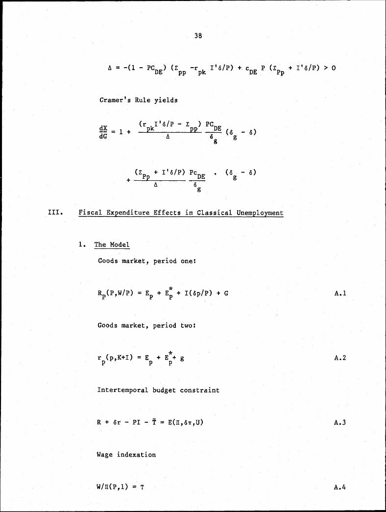
Cramer's Rule yields

g?f = 1 + dG

(r I'o/P - E ) PCDE pk PP (o - o)

b. 0 g g

(Ep + I'o/P) PeDE (a - o) + E g

ll 0 g

Fiscal Ex2enditure Effects in CLassical Unem:eloyment

1. The Model

Goods market, period one:

Goods market, period two:

* r (p,K+I) = E + E + g p p p

Intertemporal budget constraint

R + or - PI - T = E(n,o~,u)

Wage indexation

W/II(P,l) = T

A. I

A.2

A.3

A.4

39

2. Solution

- Differentiate A.l-4, substitute out u, W via A.3-4. This

results in:

Ec -l:c dP (1-PCDE)dG-opCDEdg pp pp = A.S -Ec -Ec dp -cDEPdG + {1-opc

01)dg

- pp pp-

where

Ec = E + E* - R -I' op/p2 PP PP PP PP

Ec = E + E* - r - I' op/P pp pp pp pp

* * + E o(c - c0

E) < 0 p DE

Note that symmetric expenditure patterns across countries and,

more importantly, time periods, imply

40

A.6

E + E < O, E + E < 0 pp pp pp pp

These symmetry assumptions (i.e. ITPP/rr

throughout.

= n p/n etc.) are made p

3. Terms of Trade Effects of a Transitory Increase in Government Expenditure dG>O, dg=O.

~ = l {-Ec (1-PC ) - Ec (1-opcDE)} > 0 dG ~ pp DE pp A. 7

~ = l {Ec {1-PC ) + Ec cDE P} > 0 dG ~ pP DE pp < A.B

The inequalities in A.7 and A.8 can be obtained by applying A.6.

~ c Ec - Ec Ec > 0 = Epp pp pP Pp

also !!!?. - !!P. = .!. {-Ec (1-PC ) - c dG dG ~ pp DE Epp PeDE

- Ec {1-PC ) - c pP DE Epp cDE P}

It is straightforward to s·ee that this expression is positive

. (note that all terms involving RPW cancel out).

41

4. Terms of Trade Effects of a Permanent Increase in Government Expenditure PdG = opdg > 0.

D f. dP ( dP + ~) I t e lne PdG = PdG opdg PdG = podg e c.

dP 1 {-Ec (1 PC ) c (1 o ) dG = X pp - DE + Epp - peDE

+ Ec PC - Ec opcDE} pp DE Pp

A.9

~ = ! {-Ec (1 - opc0

E) + Ec (1 - PC0

E) dG 11 pp pP A.10

Since symmetry over time implies PCDE = opcDE'

1 - PCDE - PCDE = 1-opcDE - opcDE > 0; therefore

dP ~ > dG' dG O.

Finally straightforward application of A.6 to A.9-10 shows that

Some Recent DRD Discussion Papers

237. Tax Reforms, Welfare, and Effective Tax Rates, by W. R. Thirsk.

238. Lessons from Value-Added Taxation for Developing Countries, by M. Gillis, C. Shoup and G.P. Sicat.

239. Adjustments to Policy Changes: The Case of Korea, 1960-1985, by R. Richardson and B.W. Kim.

240. Adopting a Value-Added Tax in a Developing Country, by. G.P. Sicat.

241. External Shocks and Policy Reforms in the Southern ;one: A Reassessment, by V. Corbo and J. de Melo.

242. Adjustment with a Fixed Exchange Rate: Cameroon, Cote d'Ivoire and Senegal, by S. Devarajan and J. de Melo.

243. Savings, Commodity Market Rationing and the Real Rate of Interest in China, by. A. Feltenstein, D. Lebow, and s. van Wijnbergen.

244. Labor Markets in Sudan: Their Structure and Implications for Macro­economic Adjustment, by P.R. Fallon.

245. The VAT and Services, by J.A. Kay and E.H. Davis.

246. Problems in Administering a Value-Added Tax in Developing Countries: an Overview, by M. Casanegra de Jantscher.

247. Value-Added Tax at the State Level, by S. Poddar.

248. The Importance of Trade for Developing Countries, by B. Balassa.

249. The Interaction of Domestic Distortions with Development Strategies, by Bo Balassa.

250. Economic Incentives and Agricultural Exports in Developing Countries, by B. Balassa.

251. Lessons from the Southern Cone Policy Reforms, by V. Corbo and J. de Melo.

252. On the Progressivity of Commodity Taxation, by s. Yitzhaki.

253. A Full Employment Economy and its Responses to External Shocks: The Labor Market in Egypt from World War II, by B. Hansen.

254. Next Steps in the Hungarian Economic Reform, by B. Balassa.

255. On the Progressivity of Commodity Taxation, by S. Yitzhaki.