drawdowns, drawups, their joint distributions, detection ...jrojo/pasi/lectures/oly 3.pdf · joint...
TRANSCRIPT
OutlineIntroduction
Joint Distribution of Drawdown and DrawupTransient signal detection
Maximum Drawdown ProtectionThanks toReference
Conclusion Remarks
Drawdowns, Drawups, their joint distributions, detection andfinancial risk management
June 2, 2010
Drawdowns, Drawup, their joint distributions, detection and financial risk management
OutlineIntroduction
Joint Distribution of Drawdown and DrawupTransient signal detection
Maximum Drawdown ProtectionThanks toReference
Conclusion Remarks
Introduction
Joint Distribution of Drawdown and DrawupThe cases a = bThe cases a > bThe cases a < b
Transient signal detection
Maximum Drawdown ProtectionInsuring against drawing down before drawing upRobust replicationSemi-robust hedges
Thanks to
Conclusion Remarks
Drawdowns, Drawup, their joint distributions, detection and financial risk management

OutlineIntroduction
Joint Distribution of Drawdown and DrawupTransient signal detection
Maximum Drawdown ProtectionThanks toReference
Conclusion Remarks
Motivation
I The price of a stock or index is fluctuate, and may have a big drop or a big rallyover a period [0,T].
I The present decrease from the historical highI The present increase over the historical low
01−Jan−2007 19−Dec−2007 05−Dec−2008 22−Nov−2009600
800
1000
1200
1400
1600S&P500, 2007 − Now
Historical HighSP500Historical Low
Drawdowns, Drawup, their joint distributions, detection and financial risk management

OutlineIntroduction
Joint Distribution of Drawdown and DrawupTransient signal detection
Maximum Drawdown ProtectionThanks toReference
Conclusion Remarks
Mathematical Definitions
I A stochastic process {Xt; t ≥ 0}.I Its drawdown and drawup processes.
DDt = sups≤t
Xs−Xt, DUt = Xt− infs≤t
Xs.
I Drawdowns and drawups.
TD(a) = inf{t ≥ 0|DDt ≥ a},TU(b) = inf{t ≥ 0|DUt ≥ b}.
The goal: characterize the probability Px(TD(a)≤ TU(b)∧T).
Drawdowns, Drawup, their joint distributions, detection and financial risk management

OutlineIntroduction
Joint Distribution of Drawdown and DrawupTransient signal detection
Maximum Drawdown ProtectionThanks toReference
Conclusion Remarks
The cases a = bThe cases a > bThe cases a < b
The first range time ρ(a) = TD(a)∧TU(a)
0 0.1 0.2 0.3 0.4 0.5 0.6 0.7 0.8 0.9 1−0.2
−0.15
−0.1
−0.05
0
0.05
0.1
0.15
Time t
Xt
sups<=t
Xs
Xt
infs<=t
Xs
0.3
ρ(0.3)
Drawdowns, Drawup, their joint distributions, detection and financial risk management

OutlineIntroduction
Joint Distribution of Drawdown and DrawupTransient signal detection
Maximum Drawdown ProtectionThanks toReference
Conclusion Remarks
The cases a = bThe cases a > bThe cases a < b
Probability distribution
I On {TD(a)≤ TU(a)}, XTD(a) ∈ [−a,0).I It suffices to determine
P0(TD(a) ∈ dt,TU(a) > t,Xt ∈ du), −a≤ u < 0.
I Connection with the hitting probability
P0(TD(a) ∈ dt,TU(a) > t,Xt ∈ du)
= P0(τu ∈ dt,sups≤t
Xs ∈ du+a)
=∂
∂aP0(τu ∈ dt,sup
s≤tXs < u+a)du
=∂
∂aP0(τu ∈ dt,τu+a > t)du.
I We have a closed-form formula for P0(TD(a)≤ TU(a)∧T) under driftedBrownian motion dynamics. (RW is similar)
Drawdowns, Drawup, their joint distributions, detection and financial risk management
OutlineIntroduction
Joint Distribution of Drawdown and DrawupTransient signal detection
Maximum Drawdown ProtectionThanks toReference
Conclusion Remarks
The cases a = bThe cases a > bThe cases a < b
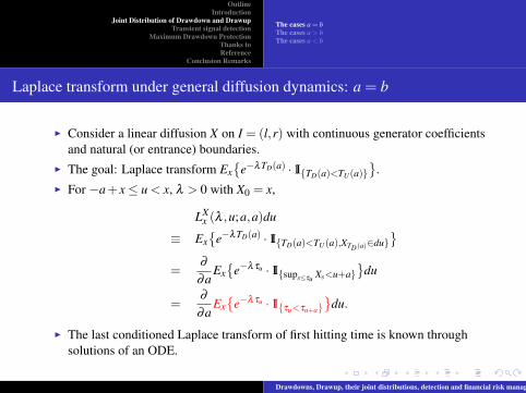
Laplace transform under general diffusion dynamics: a = b
I Consider a linear diffusion X on I = (l,r) with continuous generator coefficientsand natural (or entrance) boundaries.
I The goal: Laplace transform Ex{
e−λTD(a) ·1I{TD(a)<TU(a)}}
.I For −a+ x≤ u < x, λ > 0 with X0 = x,
LXx (λ ,u;a,a)du
≡ Ex{
e−λTD(a) ·1I{TD(a)<TU(a),XTD(a)∈du}}
=∂
∂aEx{
e−λτu ·1I{sups≤τu Xs<u+a}}
du
=∂
∂aEx{
e−λτu ·1I{τu<τu+a}}
du.
I The last conditioned Laplace transform of first hitting time is known throughsolutions of an ODE.
Drawdowns, Drawup, their joint distributions, detection and financial risk management
OutlineIntroduction
Joint Distribution of Drawdown and DrawupTransient signal detection
Maximum Drawdown ProtectionThanks toReference
Conclusion Remarks
The cases a = bThe cases a > bThe cases a < b
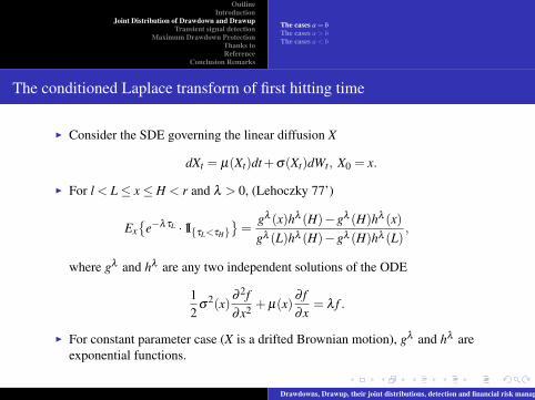
The conditioned Laplace transform of first hitting time
I Consider the SDE governing the linear diffusion X
dXt = µ(Xt)dt +σ(Xt)dWt, X0 = x.
I For l < L≤ x≤ H < r and λ > 0, (Lehoczky 77’)
Ex{
e−λτL ·1I{τL<τH}}
=gλ (x)hλ (H)−gλ (H)hλ (x)gλ (L)hλ (H)−gλ (H)hλ (L)
,
where gλ and hλ are any two independent solutions of the ODE
12
σ2(x)
∂ 2f∂x2 + µ(x)
∂ f∂x
= λ f .
I For constant parameter case (X is a drifted Brownian motion), gλ and hλ areexponential functions.
Drawdowns, Drawup, their joint distributions, detection and financial risk management
OutlineIntroduction
Joint Distribution of Drawdown and DrawupTransient signal detection
Maximum Drawdown ProtectionThanks toReference
Conclusion Remarks
The cases a = bThe cases a > bThe cases a < b
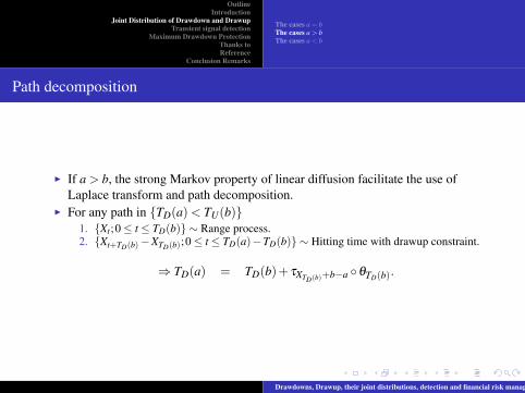
Path decomposition
I If a > b, the strong Markov property of linear diffusion facilitate the use ofLaplace transform and path decomposition.
I For any path in {TD(a) < TU(b)}1. {Xt;0≤ t ≤ TD(b)} ∼ Range process.2. {Xt+TD(b)−XTD(b);0≤ t ≤ TD(a)−TD(b)} ∼ Hitting time with drawup constraint.
⇒ TD(a) = TD(b)+ τXTD(b)+b−a ◦θTD(b).
Drawdowns, Drawup, their joint distributions, detection and financial risk management

OutlineIntroduction
Joint Distribution of Drawdown and DrawupTransient signal detection
Maximum Drawdown ProtectionThanks toReference
Conclusion Remarks
The cases a = bThe cases a > bThe cases a < b
Illustration of a Brownian sample path with a = 0.4,b = 0.2
0 0.1 0.2 0.3 0.4 0.5 0.6 0.7 0.8 0.9 1
−0.3
−0.25
−0.2
−0.15
−0.1
−0.05
0
0.05
0.1
Brownian motion Xt=0.1t+0.2W
t, t∈[0,1]; T
D(0.4)∧ 1<T
U(0.2)∧1
Time t
Xt
sups<=t
Xs
Xt
infs<=t
Xs
0.2
P
TD
(0.2)
0 0.1 0.2 0.3 0.4 0.5 0.6 0.7 0.8 0.9 1
−0.3
−0.25
−0.2
−0.15
−0.1
−0.05
0
0.05
0.1
Brownian motion Xt=0.1t+0.2W
t, t∈[0,1]; T
D(0.4)∧ 1<T
U(0.2)∧1
Time t
Xt
sups<=t
Xs
Xt
infs<=t
Xs
0.2
P
TD
(0.2) TD
(0.4)
Q
0.4
Drawdowns, Drawup, their joint distributions, detection and financial risk management

OutlineIntroduction
Joint Distribution of Drawdown and DrawupTransient signal detection
Maximum Drawdown ProtectionThanks toReference
Conclusion Remarks
The cases a = bThe cases a > bThe cases a < b
Laplace transform a > b
I Recall that on {TD(a) < TU(b)} with a > b,
TD(a) = TD(b)+ τXTD(b)+b−a ◦θTD(b)
I Conditioning on {XTD(b) = u},
Ex{
e−λτu+b−a◦θTD(b) ·1I{τu+b−a◦θTD(b)<TU(b)◦θTD(b)}|XTD(b) = u}
= Eu{
e−λτu+b−a ·1I{τu+b−a<TU(b)}}.
I For −a+ x < u < x, λ > 0 with X0 = x,
LXx (λ ,u;a,b)du
≡ Ex{
e−λTD(a) ·1I{TD(a)<TU(b),XTD(b)∈du}}
= LXx (λ ,u;b,b) ·Eu
{e−λτu+b−a ·1I{τu+b−a<TU(b)}
}︸ ︷︷ ︸The strong Markov property
du.
Drawdowns, Drawup, their joint distributions, detection and financial risk management

OutlineIntroduction
Joint Distribution of Drawdown and DrawupTransient signal detection
Maximum Drawdown ProtectionThanks toReference
Conclusion Remarks
The cases a = bThe cases a > bThe cases a < b
The strong Markov property and discrete approximation
I Conditioning on{XTD(b) = u}, partition theinterval [u−a+b,u] inton subintervals with equallength ∆ = (a−b)/n.
I Use conditioned hittingtimes to approximate.
I Pass to the limit. Thecontinuity of the samplepath and boundedconvergence theoremjustifies this.
0.45 0.5 0.55 0.6 0.65
−0.3
−0.25
−0.2
−0.15
−0.1
−0.05
0
0.05
0.1
Time t
Xt
Brownian motion Xt=0.1t+0.2W
t, t∈[T
D(0.2),T
D(0.4)]
u−4Δ
P
Q
u−Δ
u−2Δ
u−3Δ
u−Δ+b
u−2Δ+b
u−3Δ+b
u−4Δ+b
u
TD
(0.2) TD
(0.4)
Drawdowns, Drawup, their joint distributions, detection and financial risk management

OutlineIntroduction
Joint Distribution of Drawdown and DrawupTransient signal detection
Maximum Drawdown ProtectionThanks toReference
Conclusion Remarks
The cases a = bThe cases a > bThe cases a < b
Path decomposition
I Relationship between Laplace transforms
Ex{
e−λTD(a) ·1I{TD(a)<TU(b)}}
= Ex{
e−λTD(a)}−Ex{
e−λTD(a) ·1I{TD(a)>TU(b)}}
I To get the very last Laplace transform, observe that on {TD(a) > TU(b)},
TD(a) = TU(b)+TD(a)◦θTU(b).
I Using strong Markov property of linear diffusion
Ex{
e−λTD(a)◦θTU (b) |XTU(b)}
= EXTU (b)
{e−λTD(a)}.
I We can use reflection to find
Ex{
e−λTU(b) ·1I{TD(a)>TU(b),XTU (b)∈du}}.
Drawdowns, Drawup, their joint distributions, detection and financial risk management

OutlineIntroduction
Joint Distribution of Drawdown and DrawupTransient signal detection
Maximum Drawdown ProtectionThanks toReference
Conclusion Remarks
The cases a = bThe cases a > bThe cases a < b
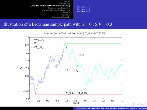
Illustration of a Brownian sample path with a = 0.15,b = 0.3
0 0.1 0.2 0.3 0.4 0.5 0.6 0.7 0.8 0.9 1−0.1
−0.05
0
0.05
0.1
0.15
0.2
0.25
0.3
Time t
Xt
Brownian motion Xt=0.1t+0.2W
t, t∈ [0,1]; T
D(0.3)∧1<T
U(0.15)∧1
sups<=t
Xs
Xt
infs<=t
Xs P
TU
(0.3)
0.3
0 0.1 0.2 0.3 0.4 0.5 0.6 0.7 0.8 0.9 1−0.1
−0.05
0
0.05
0.1
0.15
0.2
0.25
0.3
Time t
Xt
Brownian motion Xt=0.1t+0.2W
t, t∈ [0,1]; T
D(0.3)∧1<T
U(0.15)∧1
sups<=t
Xs
Xt
infs<=t
Xs P
TU
(0.3)
0.3 Q
TD
(0.15)
0.15
Drawdowns, Drawup, their joint distributions, detection and financial risk management
OutlineIntroduction
Joint Distribution of Drawdown and DrawupTransient signal detection
Maximum Drawdown ProtectionThanks toReference
Conclusion Remarks
The cases a = bThe cases a > bThe cases a < b
Illustration of a Brownian sample path with a = 0.15,b = 0.3
0 0.1 0.2 0.3 0.4 0.5 0.6 0.7 0.8 0.9 1−0.1
−0.05
0
0.05
0.1
0.15
0.2
0.25
0.3
Time t
Xt
Brownian motion Xt=0.1t+0.2W
t, t∈ [0,1]; T
D(0.3)∧1<T
U(0.15)∧1
sups<=t
Xs
Xt
infs<=t
Xs P
TU
(0.3)
0.3
0 0.1 0.2 0.3 0.4 0.5 0.6 0.7 0.8 0.9 1−0.1
−0.05
0
0.05
0.1
0.15
0.2
0.25
0.3
Time t
Xt
Brownian motion Xt=0.1t+0.2W
t, t∈ [0,1]; T
D(0.3)∧1<T
U(0.15)∧1
sups<=t
Xs
Xt
infs<=t
Xs P
TU
(0.3)
0.3 Q
TD
(0.15)
0.15
Drawdowns, Drawup, their joint distributions, detection and financial risk management

OutlineIntroduction
Joint Distribution of Drawdown and DrawupTransient signal detection
Maximum Drawdown ProtectionThanks toReference
Conclusion Remarks
Detection of two-sided alternatives
I We sequentially observe a process {ξt} with the following dynamics:
dXt =
dwt t < τ
α(Xt)dt +σ(Xt)dwtor
−α(Xt)dt +σ(Xt)dwt
T ≥ t ≥ τ
I probability of misidentification
P0,+x (TD(a) < TU(b)∧T) =
∫∞
0P0,+
x (TD(a) < TU(b)∧ t) ·λe−λ tdt
=∫
∞
0e−λ tP0,+
x (TD(a) ∈ dt,TU(b) > t)dt
= LX0,+
x (λ ;a,b), (1)
Drawdowns, Drawup, their joint distributions, detection and financial risk management

OutlineIntroduction
Joint Distribution of Drawdown and DrawupTransient signal detection
Maximum Drawdown ProtectionThanks toReference
Conclusion Remarks
Detection of two-sided alternatives(cont)
I aggregate probability of misidentification∫Pτ,+
y (TD(a)◦θ(τ) < TU(b)◦θ(τ)∧T)fXτ(y|x)dy (2)
=∫
LX0,+
y (λ ,a,b)fXτ(y|x)dy,
Drawdowns, Drawup, their joint distributions, detection and financial risk management

OutlineIntroduction
Joint Distribution of Drawdown and DrawupTransient signal detection
Maximum Drawdown ProtectionThanks toReference
Conclusion Remarks
Insuring against drawing down before drawing upRobust replicationSemi-robust hedges
Digital call insurance
I Financial assets are risky.
01−Jan−2007 19−Dec−2007 05−Dec−2008 22−Nov−2009600
800
1000
1200
1400
1600S&P500, 2007 − Now
Historical HighSP500Historical Low
I A digital call that pays 1I{TD(K)≤TU(K)∧T} can be perceived as an insuranceagainst adverse movement in the market.
Drawdowns, Drawup, their joint distributions, detection and financial risk management
OutlineIntroduction
Joint Distribution of Drawdown and DrawupTransient signal detection
Maximum Drawdown ProtectionThanks toReference
Conclusion Remarks
Insuring against drawing down before drawing upRobust replicationSemi-robust hedges
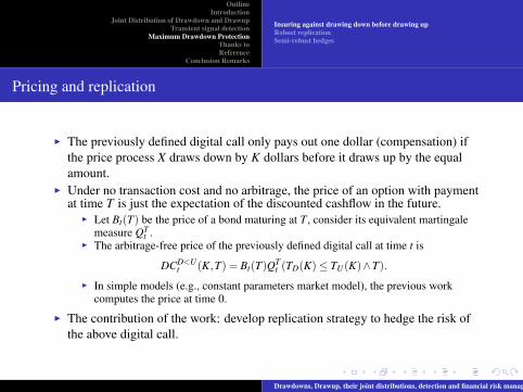
Pricing and replication
I The previously defined digital call only pays out one dollar (compensation) ifthe price process X draws down by K dollars before it draws up by the equalamount.
I Under no transaction cost and no arbitrage, the price of an option with paymentat time T is just the expectation of the discounted cashflow in the future.
I Let Bt(T) be the price of a bond maturing at T , consider its equivalent martingalemeasure QT
t .I The arbitrage-free price of the previously defined digital call at time t is
DCD<Ut (K,T) = Bt(T)QT
t (TD(K)≤ TU(K)∧T).
I In simple models (e.g., constant parameters market model), the previous workcomputes the price at time 0.
I The contribution of the work: develop replication strategy to hedge the risk ofthe above digital call.
Drawdowns, Drawup, their joint distributions, detection and financial risk management
OutlineIntroduction
Joint Distribution of Drawdown and DrawupTransient signal detection
Maximum Drawdown ProtectionThanks toReference
Conclusion Remarks
Insuring against drawing down before drawing upRobust replicationSemi-robust hedges
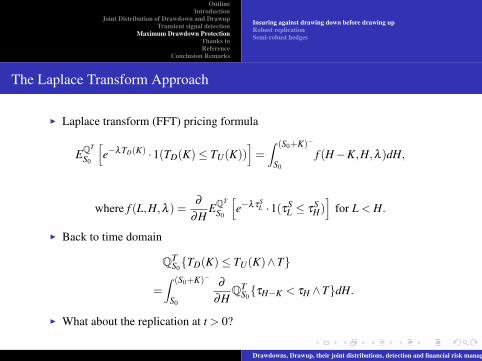
The Laplace Transform Approach
I Laplace transform (FFT) pricing formula
EQT
S0
[e−λTD(K) ·1(TD(K)≤ TU(K))
]=∫ (S0+K)−
S0
f (H−K,H,λ )dH,
where f (L,H,λ ) =∂
∂HEQT
S0
[e−λτS
L ·1(τSL ≤ τ
SH)]
for L < H.
I Back to time domain
QTS0{TD(K)≤ TU(K)∧T}
=∫ (S0+K)−
S0
∂
∂HQT
S0{τH−K < τH ∧T}dH.
I What about the replication at t > 0?
Drawdowns, Drawup, their joint distributions, detection and financial risk management

OutlineIntroduction
Joint Distribution of Drawdown and DrawupTransient signal detection
Maximum Drawdown ProtectionThanks toReference
Conclusion Remarks
Insuring against drawing down before drawing upRobust replicationSemi-robust hedges
Model-free Decomposition
I Let Xt, Mt and mt be spot price, the historical high and the historical low at timet ∈ [0,T] of the underlying, respectively.
I On any path in the event {TD(K)≤ TU(K)∧T}, at t < TD(K)∧TU(K),I If the spot does not reach a new high by TD(K), MTD(K) = Mt .I Otherwise, MTD(K) ∈ (Mt,mt +K).
I Replicate payoff based on the historical high when there is a crash: MTD(K)
1I{TD(K)≤TU(K)∧T}
=1I{TD(K)=τMTD(K)−K≤T,MTD(K)∈[Mt ,mt+K)}
=1I{τMt−K≤T,MτMt−K =Mt}
+∫ (mt+K)−
M+t
1I{τH−K≤T}δ (MτH−K −H)dH.
I Find instruments with desired payoffs.
Drawdowns, Drawup, their joint distributions, detection and financial risk management

OutlineIntroduction
Joint Distribution of Drawdown and DrawupTransient signal detection
Maximum Drawdown ProtectionThanks toReference
Conclusion Remarks
Insuring against drawing down before drawing upRobust replicationSemi-robust hedges
Hedging instruments
I An one-touch knockout is a double barrier digital option with a (low) in-barrierL and a (high) out-barrier H, the price of this options at time t before itsmaturity date T is
OTKOt(L,H,T) =Bt(T)QTt (τL ≤ τH ∧T)
=Bt(T)QTt (τL ≤ T,MτL < H).
I The payoff indicator of an one-touch knockout can be modified
OTKOt(L,H+,T) = Bt(T)QTt (τL ≤ T,MτL ≤ H).
I A touch-upper-first down-and-in claim is a spread of one-touch knockouts. Ithas a low barrier L and a high barrier H.
TUFDIt(L,H,T) = limε→0+
OTKOt(L,H + ε,T)−OTKOt(L,H,T)ε
=Bt(T)EQT
t [1I{τL≤T}δ (MτL −H)],
which pays one dollar at expiry if and only if the spot touches the upper barrierH and then hits L from above before T .
Drawdowns, Drawup, their joint distributions, detection and financial risk management

OutlineIntroduction
Joint Distribution of Drawdown and DrawupTransient signal detection
Maximum Drawdown ProtectionThanks toReference
Conclusion Remarks
Insuring against drawing down before drawing upRobust replicationSemi-robust hedges
Semi-static replication of one-touch knockouts
I Although the previous replication is fairly robust (no model assumption), theinstruments used are rather exotic.
I Under skip-freedom and symmetry assumption, any one-touch knockout can bereplicated by single barrier one-touch options: OTt(B,T) = Bt(T)QT
t (τB ≤ T).I We assume that the barriers of an one-touch knockout are skip-free, and when X
exit the corridor (L,H), the risk-neutral probability of hitting Xt−∆ before T isthe same as the risk-neutral probability of hitting Xt +∆ before T , for any ∆≥ 0.This is satisfied by dXt = αtdWt with dαtdWt = 0.
I Then, . . .
Drawdowns, Drawup, their joint distributions, detection and financial risk management
OutlineIntroduction
Joint Distribution of Drawdown and DrawupTransient signal detection
Maximum Drawdown ProtectionThanks toReference
Conclusion Remarks
Insuring against drawing down before drawing upRobust replicationSemi-robust hedges
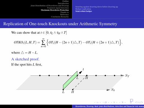
Replication of One-touch Knockouts under Arithmetic Symmetry
We can show that at t ∈ [0,τL∧ τH ∧T]
OTKOt(L,H,T) =∞
∑n=0
{OTt(H− (2n+1)4,T)−OTt(H +(2n+1)4,T)
},
where 4= H−L.
A sketched proof.If the spot hits L first,
ST
t
S0L H
L H
Drawdowns, Drawup, their joint distributions, detection and financial risk management

OutlineIntroduction
Joint Distribution of Drawdown and DrawupTransient signal detection
Maximum Drawdown ProtectionThanks toReference
Conclusion Remarks
Insuring against drawing down before drawing upRobust replicationSemi-robust hedges
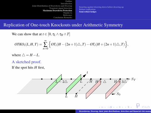
Replication of One-touch Knockouts under Arithmetic Symmetry
We can show that at t ∈ [0,τL∧ τH ∧T]
OTKOt(L,H,T) =∞
∑n=0
{OTt(H− (2n+1)4,T)−OTt(H +(2n+1)4,T)
},
where 4= H−L.
A sketched proof.If the spot hits H first,
ST
t
S0L H
L H H +△
Drawdowns, Drawup, their joint distributions, detection and financial risk management

OutlineIntroduction
Joint Distribution of Drawdown and DrawupTransient signal detection
Maximum Drawdown ProtectionThanks toReference
Conclusion Remarks
Insuring against drawing down before drawing upRobust replicationSemi-robust hedges
Replication of One-touch Knockouts under Arithmetic Symmetry
We can show that at t ∈ [0,τL∧ τH ∧T]
OTKOt(L,H,T) =∞
∑n=0
{OTt(H− (2n+1)4,T)−OTt(H +(2n+1)4,T)
},
where 4= H−L.
A sketched proof.If the spot hits L first,
ST
t
S0L H
L H H +△L− 2△
Drawdowns, Drawup, their joint distributions, detection and financial risk management
OutlineIntroduction
Joint Distribution of Drawdown and DrawupTransient signal detection
Maximum Drawdown ProtectionThanks toReference
Conclusion Remarks
Insuring against drawing down before drawing upRobust replicationSemi-robust hedges
Replication of One-touch Knockouts under Arithmetic Symmetry
We can show that at t ∈ [0,τL∧ τH ∧T]
OTKOt(L,H,T) =∞
∑n=0
{OTt(H− (2n+1)4,T)−OTt(H +(2n+1)4,T)
},
where 4= H−L.
A sketched proof.If the spot hits H first,
ST
t
S0L H
L H H +△L− 2△ H + 3△
Drawdowns, Drawup, their joint distributions, detection and financial risk management

OutlineIntroduction
Joint Distribution of Drawdown and DrawupTransient signal detection
Maximum Drawdown ProtectionThanks toReference
Conclusion Remarks
Insuring against drawing down before drawing upRobust replicationSemi-robust hedges
Semi-Robust Replication of Digital Call on Maximum Drawdown (Carr)
I The maximum drawdown MDT = sups∈[0,T] DDs, is commonly used as ameasure of the risk of holding the underlying asset over a period [0,T].
I A risk adverse investor or a portfolio manager can get protection against a lossfrom the market if he or she holds a claim which pays 1(MDT ≥ K), for somestrike K > 0.
I The maximum drawdown and the maximum drawup over a period [0,T] arerelated to two stopping times: for K > 0
TD(K) = inf{t ≥ 0,DDt ≥ K}, TU(K) = inf{t ≥ 0,DUt ≥ K}.
Let us denote by MUT = sups∈[0,T] DUs, then
{MDT ≥ K}= {TD(K)≤ T}, {MUT ≥ K}= {TU(K)≤ T}.
I Introduce another digital call for K > 0:I Digital call on maximum drawdown
DCMDt (K,T) = Bt(T)QT
t {TD(K)≤ T}.
Drawdowns, Drawup, their joint distributions, detection and financial risk management
OutlineIntroduction
Joint Distribution of Drawdown and DrawupTransient signal detection
Maximum Drawdown ProtectionThanks toReference
Conclusion Remarks
Insuring against drawing down before drawing upRobust replicationSemi-robust hedges
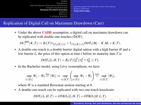
Replication of Digital Call on Maximum Drawdown (Carr)
I Under the above CAHS assumption, a digital call on maximum drawdown canbe replicated with double-one-touches (DOT):
DCMDt (K,T) := Bt(T)1{TD(K)≤t}+1{TD(K)>t}DOTt(Mt−K,Mt +K,T).
I A double-one-touch is a double barrier digital option with a high barrier H and alow barrier L, the price of this option at time t before its maturity date T is
DOTt(L,H,T) = Bt(T)QTt {τ
SL ∧ τ
SH ≤ T}.
I In the Bachelier model, using Levy isomorphism, we have
sups∈[0,t]
Ws−Wtlaw= |Wt| ⇒ sup
t∈[0,T]
(sup
s∈[0,t]Ws−Wt
)law= sup
t∈[0,T]|Wt|,
where W is a standard Brownian motion starting at 0.I A double-one-touch can be replicated with two one-touch knockouts:
DOTt(L,H,T) = OTKOt(L,H,T)+OTKOt(H,L,T).
Drawdowns, Drawup, their joint distributions, detection and financial risk management
OutlineIntroduction
Joint Distribution of Drawdown and DrawupTransient signal detection
Maximum Drawdown ProtectionThanks toReference
Conclusion Remarks
Insuring against drawing down before drawing upRobust replicationSemi-robust hedges
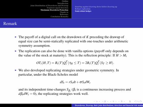
Remark
I The payoff of a digital call on the drawdown of K preceding the drawup ofequal size can be semi-statically replicated with one-touches under arithmeticsymmetry assumption.
I The replication can also be done with vanilla options (payoff only depends onthe value of the stock at maturity). This is the reflection principle: If H > Mt
OTt(H,T) = Bt(T)QTt (τH ≤ T) = 2Bt(T)QT
t (ST ≥ H).
I We also developed replicating strategies under geometric symmetry. Inparticular, under the Black-Scholes model
dSt = rStdt +σStdWt
and its independent time-changes Sβt(βt is a continuous increasing process and
dβtdWt = 0), the replicating strategies work well.
Drawdowns, Drawup, their joint distributions, detection and financial risk management
OutlineIntroduction
Joint Distribution of Drawdown and DrawupTransient signal detection
Maximum Drawdown ProtectionThanks toReference
Conclusion Remarks
Thanks to
I Hongzhong Zhang*I Peter CarrI Libor PospisilI Jan Vecer
Drawdowns, Drawup, their joint distributions, detection and financial risk management
OutlineIntroduction
Joint Distribution of Drawdown and DrawupTransient signal detection
Maximum Drawdown ProtectionThanks toReference
Conclusion Remarks
Reference
I The joint distribution of drawdown and drawup:I Zhang, H., Hadjiliadis, O.: Drawdowns and rallies in a finite time horizon, accepted
by Methodology and Computing in Applied Probability, special issue (2010).I Pospisil, L., Vecer, J., Hadjiliadis, O.: Formulas for stopped diffusion processes with
stopping times based on drawdowns and drawups, Stochastic processes and theirapplications 119(8), 2010.
I Zhang, H., Hadjiliadis, O.: Formulas for the Laplace transform of stopping timesbased on drawdowns and drawups, submitted to Annals of Applied Probability on04-24-09, revised on 02-18-10.
I Maximum drawdown protection:I Carr, P., Zhang, H., Hadjiliadis, O.: Insuring against maximum drawdown and
drawing down before drawing up, to be submitted to Finance and Stochastics.
Drawdowns, Drawup, their joint distributions, detection and financial risk management

OutlineIntroduction
Joint Distribution of Drawdown and DrawupTransient signal detection
Maximum Drawdown ProtectionThanks toReference
Conclusion Remarks
Summary
I We study drawdown and drawup processes in this work.I The probability that a drawdown of size a precedes a drawup of size b is fully
characterized for biased simple random walk, drifted Brownian motion andmore general linear diffusion with continuous generator coefficients.
I Digital insurance can be considered in terms of drawdowns and drawups.Pricing can be done analytically for classical models.
I Robust and semi-robust replicating strategies of the digital insurance aredeveloped. We considered both the arithmetic symmetry and the more involvedgeometric symmetry in the paper. These strategies are robust to independentcontinuous time-changes.
I The drawup of log-likelihood ratio process has optimal property when used as ameans of detecting abrupt changes.
I We proved the asymptotic optimality of N-CUSUM stopping rule in themulti-source observation setting. In the paper we considered both the Brownianmotion system and the discrete-time observation system.
Drawdowns, Drawup, their joint distributions, detection and financial risk management