drainage salmonid study - king county, washington

3 – 1

CHAPTER 3

Identification of an Index of Salmonid Abundance in

Agricultural Waterways

3.1 Introduction to Abundance Index Development (Goal 2)

King County DNRP, as part of its regulatory and management activities, has an ongoing interest

in determining presence/absence or abundance of salmonids in various waterways throughout the

county. Agricultural waterways typically have heavy cover and limited visibility relative to

more „typical‟ salmon bearing channels and effective methods for evaluation of fish abundance

in these channels are not clearly understood. Despite the difficulty of sampling fish in

agricultural watercourses, these habitats are known to be used by various native fish species. As

a result, Goal two of this study was to identify an index of salmonid abundance applicable across

the range of habitat conditions observed in the County‟s agricultural waterways. This chapter is

focused on the evaluation and utility of various fish collection methods for effective indexing of

salmonid abundance in agricultural waterways.

With the assistance of KCDNRP staff, the following research hypothesis was posed in relation to

this study component:

Hypothesis 1: Related to the collection of juvenile salmonids, sampling bias does

not vary across sampling procedures (including electrofishing and various

trapping methods).

Ney (1993) summarizes a common premise in population estimation in which, if absolute

abundance of a fish stock is found to be highly correlated to catch-per-unit-effort (CPUE) of a

particular sampling technique or set of techniques, then those measures of relative abundance

(CPUE) can be used as an accurate index of fish density or population size. The focus of this

study component was to evaluate the utility of catch data based on various fish sampling

techniques as indices of salmonid abundance or density within agricultural waterways.

Professional experience and consultations with KCDNRP staff suggested that backpack

electrofishing and trapping are the most effective techniques for sampling juvenile salmonids

over the wide range of habitat conditions found within agricultural waterways. Monitoring

methods selected for this study therefore included backpack electrofishing and four trap

configurations (empty, baited, lighted and baited/lighted). Additional methods (snorkel surveys

and seining) were considered but not applied due to dense aquatic vegetation and limited

visibility in most of these channels, and previous experience of KCDNRP staff.

3 – 2

3.2 Study Area

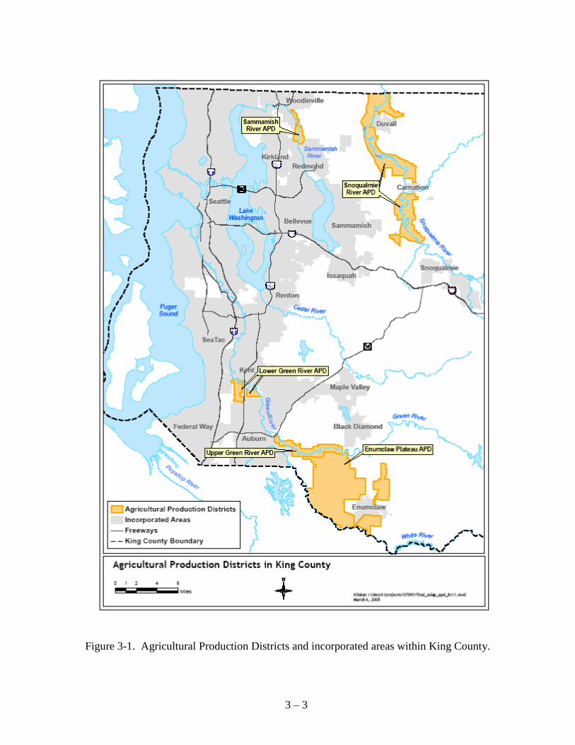
This study was conducted in waterways in or near King County's Agricultural Production

Districts (APDs), which are composed of approximately 40,600 acres (16,430 hectares) zoned

for agricultural use (Figure 3-1). An estimated 483 kilometers (300 miles) of watercourses,

excluding the mainstems (and braids) of the major rivers, flow through King County‟s five APDs

(Lower Green River, Upper Green River, Enumclaw, Sammamish, and Snoqualmie). The APDs

are located almost exclusively on the floodplains of major rivers, with the exception of the

Enumclaw Plateau APD. However, agricultural activities in the Enumclaw Plateau APD occur

on similar extremely flat land, and often affect channels and riparian zones with similar

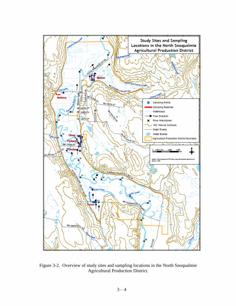
characteristics to those on the valley floors surrounding large rivers. Sampling for this study

took place in waterways within the Snoqualmie (Figure 3-2, Figure 3-3, Figure 3-4 and Figure 3-

5) APD at locations believed to be representative of those found throughout the county‟s five

APDs.

3 – 3

Figure 3-1. Agricultural Production Districts and incorporated areas within King County.

3 – 4

Figure 3-2. Overview of study sites and sampling locations in the North Snoqualmie

Agricultural Production District.

3 – 5

Figure 3-3. Detail of study sites and sampling locations in the northern portions of the North

Snoqualmie Agricultural Production District.

3 – 6

Figure 3-4. Detail of study sites and sampling locations in the central portions of the North


3 – 7

Figure 3-5. Detail of study sites and sampling locations in the southern portions of the North


3 -8

3.3 Methods

3.3.1 Data Collection Efforts to evaluate various sampling strategies as indices of salmonid abundance were conducted

in late summer of 2004 (August) and 2005 (September) and in the winter (January) of 2005. The

timing of late summer sampling periods1 coincided with the established „fish window‟ during

which agricultural waterway maintenance and associated defishing activities would normally

occur (King County public rule 21A-24 “Maintenance of Agricultural Ditches and Streams Used

by Salmonids” sub-section 374 (King County DDES 2001). The purpose of the winter period

was to assess any impact that seasonal differences in conditions (e.g. temperature, flows, water

levels) might have on utilization of such an index.

The design layout of study components at field sites varied by sampling period with designs

differing between the first two periods (August 2004 and January 2005) and the final period

(September 2005). The study layout during the first two sampling periods was most

representative of conditions during typical site evaluations or population surveys, whereas the

study layout during the final period was most representative of conditions that exist during

defishing and other activities normally preceding agricultural waterway maintenance activities.

Site selection criteria required that sites: 1) had similar cover and habitat characteristics along

their entire length, 2) had suitable length to establish two sub-reaches, 3) represented various

habitat (riparian vegetation) conditions and, 4) were considered likely to have sufficient numbers

of salmonids to allow for successful estimation of population size through mark-recapture

techniques based on review of past monitoring data. Consideration was also given to

accommodation of logistic constraints (e.g. limited distance between sites to allow multiple daily

visits to each) during site selection. Five sites (Turner-A, Nelson-B, Decker-A, Olney-B, and

Olney-D) were utilized for evaluation of sampling efficiency and bias, all of which were located

within the North Snoqualmie APD (Figure 3-2, Figure 3-3, Figure 3-4 and Figure 3-5).

As previously described, electrofishing and trapping were considered the most effective methods

for sampling juvenile salmonids within agricultural waterways. Monitoring methods selected for

this study therefore included backpack electrofishing and four trap configurations (empty, baited,

lighted, and baited/lighted). Sub-reaches were established at each site using 0.6cm (0.25 inch)

mesh block nets placed at both the upstream and the downstream ends of the selected reach.

Block nets were equipped with float lines on the surface and were set into the available bottom

substrate to meet the assumptions of a closed system necessary for the study (Peterson et al.

2005).

1 For the purpose of this report the terms „event‟ and „period‟ will be distinguishable as follows:

* Event describes a single sampling technique used a single time (e.g. one electrofishing pass, one trap-day OR

one trap-night).

* Period will be used to represent a series of dates which encompasses numerous sampling events (e.g. The

August, 2004 sampling period encompasses multiple days and includes numerous shocking and trapping

events).

3 -9

Repeated sampling was conducted (multi-pass electrofishing and multiple day/nights of trapping)

with replacement. Unmarked fish captured during each pass were marked by clipping one pelvic

fin prior to their release back into the study reach. An estimate of salmonid population size

within each reach was determined using standard mark-recapture estimation methods (see Van

Den Avyle (1993) for a review and discussion of applicable methods). This approach allowed

for estimation of initial population size2, and back calculation of capture efficiency and sampling

bias related to each electrofishing pass/trapping event (e.g. each trap-day or trap-night).

Electrofishing was conducted using a Smith Root, Inc. model 12 backpack electrofisher with a 6

foot electrode pole and an 11 inch electrode ring covered with 1/4 inch mesh netting. Fish

stunned by the electrofisher were collected either with a separate dip net or using the net covered

electrode ring; when collecting fish with the electrode ring, power to the electrode was

temporarily terminated to eliminate harm or further stress to the fish.

Trapping was conducted with standard steel mesh minnow traps 17 inches long with a 9 inch

diameter and a 1 inch access opening on each end. Trap mesh had openings 0.25 x 0.5 inches.

Traps were baited with approximately 1.5 ounces of tuna fish wrapped in mosquito netting and

lighted using 6 inch cylume light sticks. Various colors of light sticks were used depending upon

availability although an attempt was made to use a single color of light stick at each site during

each sampling event. Both bait and light sticks were attached in the center of the minnow trap

and changed each time a trap was checked and reset.

3.3.1.1 Late Summer 2004 and Winter 2005

In August of 2004 and January of 2005, two sub-reaches of equal length were established

immediately adjacent to one another at each study site by setting 3 block nets constructed of 1/8

inch mesh. The length of sub-reaches was equal at each site but varied between sites based on

the suitable length of waterway available. Length of reaches ranged from 350 to 600 feet; length

of sub-reaches ranged from 175 to 300 feet. Twelve traps were set equidistantly in the upstream

sub-reach; trap configurations were determined using a systematic random process with the

configuration of the downstream most trap selected randomly, and the remainder set in a

systematic order (empty, baited, lighted, lighted/baited). Electrofishing was conducted along the

entire length of the downstream sub-reach. In this manner, disturbances (e.g. suspended

sediment load) caused by electrofishing activity did not impact conditions within the trap sub-

reach.

Electrofishing was generally performed only once per day to ensure „best case‟ conditions (e.g.

minimal suspended sediment during sampling and opportunity for fish to re-distribute between

individual sampling events). In limited instances a sub-reach was shocked multiple times on the

final sampling date (early and late in the day) to increase numbers of fish captured or recaptured

and to improve precision of the population estimate and subsequent estimates of sampling

efficiency and bias.

2 Ideally, known numbers of hatchery salmonids would have been marked and released into test reaches for these

evaluations to provide abundant fish for capture. However, logistic (e.g. permitting and transport) and

environmental (e.g. low DO levels in the study reaches during study periods) constraints precluded the use hatchery

fish for these evaluations. This issue is addressed further in the Discussion section of this report.

3 -10

Traps were checked twice per day to evaluate potential differences in sampling efficiency and

bias between „day‟ and „night‟ conditions3. Upon completion of all trapping activities the

corresponding sub-reach was electrofished to increase numbers of fish captured or recaptured

and improve precision of the population estimate and subsequent estimates of sampling

efficiency and bias.

3.3.1.2 Late Summer 2005

During September 2005, shocking and trapping efforts were conducted in the same reach rather

than in separate sub-reaches. This was done, in part, due to relatively low numbers of fishes

captured and marked in previous efficiency/bias evaluation efforts; shocking and trapping in the

same reach allowed for a greater number of fish to be marked, a potentially more precise

population estimate, and a better subsequent evaluation of trapping efficiency and bias. The

sampled reach was established by setting block nets on each end to establish a closed population

within the reach.

Multiple pass electrofishing (two passes) was conducted during the day at each site on each date

to allow comparison of sampling effectiveness during „clean‟ and „dirty‟ conditions. The initial

electrofishing pass each day, when sediment and fish were undisturbed was characterized as a

„clean‟ shock; a subsequent electrofishing pass conducted shortly after the initial shock when

sediments were still disturbed, visibility reduced, and fish presumably lodged deeper into

available cover due to that disturbance, was characterized as a „dirty‟ shock. This scenario was

thought to reproduce conditions that exist during fish removal (“defishing”) activities preceding

agricultural waterway maintenance activities, when multiple electrofishing passes may be

completed within a short timeframe.

Consistent with earlier sampling periods, twelve traps were set equidistantly in the reach and trap

configurations were determined using the same systematic random process. Traps were

deployed late in the day and retrieved early the following morning prior to the onset of any

electrofishing effort.

3.3.2 Data Analysis For analyses, data from all salmonid species captured were pooled. This was done to allow

inclusion of data from those species rarely observed or captured in insufficient numbers to allow

for subsequent population estimation (e.g. cutthroat trout and Chinook salmon). In addition,

preliminary analysis indicated that salmonid captures by each of the four trap configurations

(empty, lighted, baited, lighted/baited) were most frequently zero or very near zero, precluding

our ability to adequately evaluate sampling effectiveness for individual trap configurations, or

independently for day versus night sampling periods. For each site and event, data from all trap

configurations was therefore pooled and subsequent analyses completed without regard to trap

configuration or time of day.

3 Due to travel logistics between sites, definition of „day‟ or „night‟ trapping events should be interpreted loosely.

Traps were typically checked and reset some time after sunrise, and again prior to sunset so that „day‟ sets did not

include all available daylight hours, a limited number of which were included in „night‟ sets.

3 -11

The CPUE observed at each site during each sampling event was used for regression analyses.

Doing so removed any effects of variable lengths and widths of sampling reaches and of variable

sampling time spent within a given reach. For the purpose of these analyses, 100 seconds of

shocking time or 360 trap-minutes (one trap x 6 hours) were considered standard units of effort.

Population estimates were obtained using Schnabel's (1938) approximation to the maximum

likelihood estimator of population, N, from multiple censuses (Ricker 1975), as adjusted by

Chapman (1952, 1954):

m

i

ii

R

MCN

1 1 (3-1)

where m is the number of sampling periods, Mi is the total number of fish marked at the start of

sampling period i, Ci is the total number of fish captured during sampling period i, and R is the

total number of recaptures during the experiment.

Approximate 95% confidence limits for this estimator were obtained by treating R as a Poisson

variable and substituting relevant limits determined by Ricker (1975; presented in Schneider

2000) for R in the equation above. This approach to calculation of confidence intervals was

considered more appropriate than more conventional approaches because the number of

recaptures (R) encountered at each site/sampling period was typically small (e.g. <25; Van Den

Avyle 1993).

Both length and width of selected study reaches varied with location and season. To standardize

data, population estimates were converted to density estimates (number of fish per 100 square

feet) for subsequent regression analyses.

Regression analysis was used to evaluate the relationship between estimated salmonid density

and CPUE. For evaluation of this relationship, salmonid density was considered the independent

variable, and CPUE the dependent variable. Since unpredictable salmonid distribution limited

the availability of usable data from some vegetative habitats comparison of independent

regressions for each habitat type was not possible. Alternatively, comparison of regression

slopes was performed between pooled data from all vegetative classes and reduced data sets with

data from specific habitats removed. This allowed inferences to be drawn regarding potential

differences in the relationship between CPUE and salmonid density across habitat types.

Paired T-tests were conducted to compare salmonid catch rates during „Clean‟ versus „Dirty‟

electrofishing passes conducted at the same site. Preliminary analysis suggested divergent

variances between the two data sets, so we assumed unequal variances between datasets when

conducting T-tests. T-tests were one-tailed and tested the hypothesis that salmonid catch rates

observed during „Dirty‟ electrofishing conditions were less than that observed during „Clean‟

electrofishing conditions.

3 -12

3.4 Results

Sampling related to this study goal was performed at a total of five sites across three sampling

periods (Table 3-1). Three different habitat regimes were sampled including predominantly

RCG (2 sites), mixed vegetation (includes both herbaceous vegetation and a moderate to

abundant RCG influence; 2 sites), and no vegetation due to recent maintenance activity (1 site).

Sampling related to this study component was not attempted in an available naturally vegetated

site due to recently observed lack of salmonids during seasonal surveys and/or the construction

of a downstream beaver dam which inundated the site to depths making sampling impossible.

Salmonids were not collected at all sites sampled, and estimation of population size or salmonid

density was not possible at all sites where salmonids were collected. During August 2004,

salmonid population estimates were possible at the Turner-A site in both the shocking and

trapping sub-reaches where populations of 303 and 458 salmonids were estimated, respectively

(details shown in Table 3-2). During the same sampling period, salmonid population estimation

was also possible within the trapped sub-reach at the Nelson-B site where 79 salmonids were

estimated to exist. In both trapped sub-reaches (Turner-A and Nelson-B sites), confidence in

population estimates were negatively impacted by low numbers (<5) of recaptured salmonids

during the experiment resulting in very wide confidence intervals around the estimates (See

Appendix 3-A).

During January 2005, salmonid population estimates were possible at the Turner-A site in both

the shocking and trapping sub-reaches where populations of 19 and 102 salmonids were

estimated, respectively (Table 3-3). In both cases the confidence in population estimates were

negatively impacted by low numbers (<5) of recaptured salmonids during the experiment

resulting in very wide confidence intervals around the estimates (See Appendix 3-A).

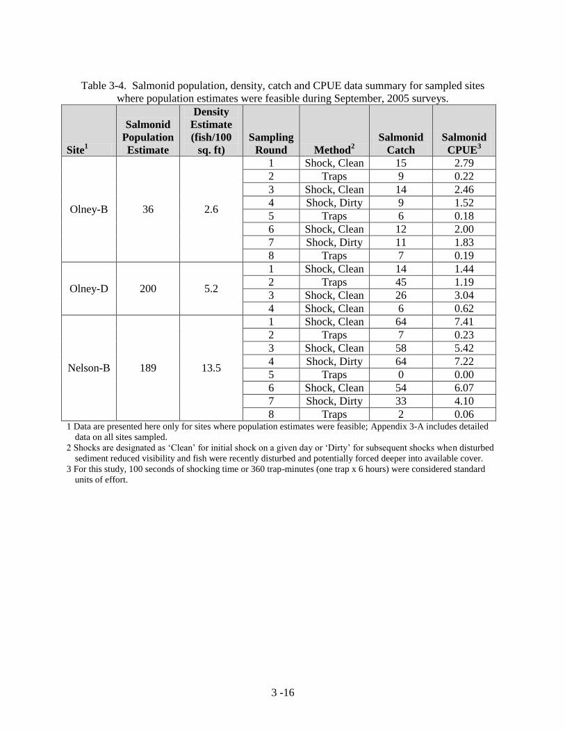
During September 2005, salmonid population estimates were possible at all sites sampled.

Based on combined sampling (shocking and trapping) at each site, salmonid population estimates

were 189, 36, and 200 at the Nelson-B, Olney-B and Olney-D sites, respectively (Table 3-4).

Unlike other sampling events, sufficient numbers (≥5) of salmonids were recaptured at all sites

during September, 2005 to allow confident estimation of population size within each sampling

reach (See Appendix 3-A).

The relationship between estimated salmonid density and electrofishing CPUE (Figure 3-6) was

much stronger than that observed between salmonid density and trap CPUE (Figure 3-7).

Electrofishing CPUE was significantly (p<0.0001) linearly related to salmonid density, and the

coefficient of determination (r2) was 0.81 indicating the strength of that relationship (Figure 3-6).

In contrast, trapping CPUE was not significantly related to salmonid density (p=0.5472) and the

relationship exhibited an r2 value of less than 0.02 (Figure 3-7). No further analysis was done

involving trap data since the initial evaluation did not reveal a significant nor apparently relevant

relationship between trap catch rates and salmonid density.

3 -13

Table 3-1. Characterization of timing and location of sampling efficiency and bias surveys (shaded blocks). Salmonid species

collected are listed; Bold print indicates that estimation of a population size was possible for a given species.

Site Name Vegetative

Habitat

August 2004 January 2005 September 2005

Electrofishing Trapping Electrofishing Trapping Combined1

Turner-A Mixed Coho, Cutthroat Coho, Cutthroat Coho, Chinook Coho, Cutthroat

Nelson-B Mixed No Salmonids Coho Coho, Chinook

Decker-A2

Reed

Canarygrass

No Fish No Salmonids

Olney-B

Reed

Canarygrass Coho, Cutthroat

Olney-D Cleaned

Coho, Cutthroat,

Chinook

Coho, Cutthroat,

Chinook Coho

1 During August, 2004 and January, 2005 electrofishing and trapping were conducted in separate sub-reaches; During September, 2005 both techniques were

„combined‟ in a single sub-reach.

2 For this particular experiment, a sub-reach at the site which was dominated by RCG was selected; this is a different habitat classification than is portrayed in

other chapters of this report when a longer, longitudinally mixed vegetative regime was sampled.

3 -14

Table 3-2. Salmonid population, density, catch and CPUE data summary for sampled sites

where population estimates were feasible during August, 2004 surveys.

Site1 Method

Salmonid

Population

Estimate

Density

Estimate

(fish/100

sq. ft)

Sampling

Round

Salmonid

Catch

Salmonid

CPUE2

Turner-A

Shock 311 8.6

1 48 3.69

2 55 3.16

3 38 3.21

Traps 458 12.7

1 6 0.41

2 4 0.15

3 12 0.64

4 4 0.14

5 3 0.15

6 1 0.03

Shock

(trap reach) 458 12.7

7 65 7.41

Nelson-B

Traps 79 4.0

1 1 0.04

2 0 0.00

3 1 0.04

4 1 0.07

5 3 0.10

6 1 0.08

Shock

(trap reach) 79 4.0

7 20 2.23 1 Data are presented here only for sites where population estimates were feasible; Appendix 3-A includes detailed

data on all sites sampled.

2 For this study, 100 seconds of shocking time or 360 trap-minutes (one trap x 6 hours) were considered standard

units of effort.

For electrofishing data only, comparison of regression slopes was performed between pooled

data from all vegetative classes and reduced data sets with data from specific habitats removed to

investigate the degree to which data from certain vegetative habitats influenced the overall

relationship. Summary information for each of those regressions is presented in Table 3-5.

Graphical representations of each regression are presented in Appendix 3-B.

For all of the reduced data sets, r2 values were increased slightly relative to that of the complete

dataset (0.84-0.87 versus 0.81; Table 3-5), suggesting that inclusion of multiple vegetative types

does introduce additional variability to the relationship. However, none of the reduced data sets

resulted in a slope significantly different from that of the complete data set (p>0.5 in all cases),

suggesting that the nature of the relationship between salmonid density and CPUE does not differ

substantially across vegetative regimes.

3 -15


where population estimates were feasible during January, 2005 surveys.

Site1 Method

Salmonid

Population

Estimate

Density

Estimate

(fish/100

sq. ft)

Sampling

Round

Salmonid

Catch

Salmonid

CPUE2

Turner-A

Shock 19 0.8

1 4 0.68

2 7 0.86

3 3 0.36

4 0 0.00

Traps 102 2.8

1 1 0.03

2 2 0.13

3 6 0.19

4 1 0.07

5 2 0.06

6 0 0.00

Shock

(trap reach) 102 2.8

7 30 2.30 1 Data are presented here only for sites where population estimates were feasible; Appendix 3-A includes detailed



units of effort.

The use of the average of multiple CPUE measurements4 rather than a single CPUE

measurement appears to provide a more reliable index of salmonid density in agricultural

waterways. When the average CPUE was regressed on estimated salmonid density, the r2 value

increased from 0.81 (for non-averaged data) to 0.92 (Table 3-5; Appendix 3-B). The slope of the

relationship using averaged data (0.452) did not differ significantly from that of the un-averaged

data (0.4179) illustrating that the nature of the relationship between CPUE or average CPUE and

salmonid density is similar.

Limited data regarding „clean‟ versus „dirty‟ electrofishing efforts was available for two sites

sampled during September, 2005 (Table 3-4). In total, six „clean‟ and four „dirty‟ electrofishing

efforts were utilized in these comparisons; Three of the four electrofishing efforts performed in

„dirty‟ conditions exhibited CPUE values lower than those observed during „clean conditions at

the same site (Figure 3-6). In the RCG dominated habitat at the Olney-B site, a paired T-test

indicated that mean electrofishing CPUE during „dirty‟ conditions was significantly less than that

observed during „clean‟ conditions (mean CPUE was 2.42 and 1.67, respectively; p=0.0367). In

contrast, at the Nelson-B site (characterized by a mixed vegetative regime), a paired T-test

indicate no significant difference in mean salmonid CPUE between „clean‟ and „dirty‟ conditions

(means 6.30 and 5.66, respectively; p=0.3831).

4 In this instance, averages were calculated for multiple electrofishing efforts performed under similar conditions

(e.g. „clean‟ or „dirty‟ shocks were considered separately) at the same site during a single sampling period (e.g.

August, 2004).

3 -16


where population estimates were feasible during September, 2005 surveys.

Site1

Salmonid

Population

Estimate

Density

Estimate

(fish/100

sq. ft)

Sampling

Round Method2

Salmonid

Catch

Salmonid

CPUE3

Olney-B 36 2.6

1 Shock, Clean 15 2.79

2 Traps 9 0.22


4 Shock, Dirty 9 1.52

5 Traps 6 0.18



8 Traps 7 0.19

Olney-D 200 5.2


2 Traps 45 1.19



Nelson-B 189 13.5


2 Traps 7 0.23



5 Traps 0 0.00



8 Traps 2 0.06 1 Data are presented here only for sites where population estimates were feasible; Appendix 3-A includes detailed


2 Shocks are designated as „Clean‟ for initial shock on a given day or „Dirty‟ for subsequent shocks when disturbed

sediment reduced visibility and fish were recently disturbed and potentially forced deeper into available cover.


units of effort.

3 -17

y = 0.4179x + 0.4096

R2 = 0.8122

Significant: p<0.0001

0.00

1.00

2.00

3.00

4.00

5.00

6.00

7.00

8.00

0.0 2.0 4.0 6.0 8.0 10.0 12.0 14.0 16.0

Estimated Density (fish/100 sq. ft)

CP

UE

(S

alm

on

ids

/10

0 s

ho

ck

se

co

nd

s)

Turner, Aug '04

Turner, Jan '05

Nelson B, Aug '04

Nelson B, 'Clean Shock', Sept '05

Nelson B, 'Dirty Shock', Sept '05

Olney A, 'Clean Shock', Sept '05

Olney A, 'Dirty Shock', Sept '05

Olney C (dredged), Sept '05

Linear (Best Fit - All Data)

Figure 3-6. Observed relationship between electrofishing (shocking) CPUE and estimated

salmonid density in agricultural waterways.

y = 0.0067x + 0.1306

R2 = 0.016

Not Significant; p=0.5472

0.00

0.20

0.40

0.60

0.80

1.00

1.20

1.40

0.0 2.0 4.0 6.0 8.0 10.0 12.0 14.0 16.0


CP

UE

(S

alm

on

ids

/ 6

tra

p h

ou

rs)

Turner, Aug '05

Turner, Jan '05

Nelson B, Aug '04

Nelson B, Sept '05

Olney A, Sept '05

Olney C, Sept '05

Linear (Best Fit - All Data)

Figure 3-7. Observed relationship between trap CPUE and estimated salmonid density in

agricultural waterways.

3 -18

Table 3-5. Summary of regression parameters relating electrofishing CPUE and salmonid

density across various combinations of vegetative habitats.

Data Included

Sample

Size

(n) r2 Intercept Slope

Slope Different from

Complete Data Set?

(p-value)

Complete Data Set –

All Vegetative Groups 23 0.8122 0.4096 0.4179 N/A

Mixed Vegetation Only 15 0.8664 0.1969 0.4407 No (p=0.642)

Mixed and RCG

Vegetation 20 0.8505 0.5819 0.4116 No (p=0.879)

Mixed Vegetation and

Cleaned 18 0.8393 -0.0166 0.4520 No (p=0.500)

Site Averaged Data Set –

All Vegetative Groups1 7 0.9230 0.4414 0.3951 No (p=0.6738)

1 „Site Averaged‟ data includes only those sites where multiple comparable electrofishing efforts were made during

the same sampling period, and regresses the average CPUE against estimated salmonid density.

3.5 Discussion

Based on the findings of this study, electrofishing CPUE appears to provide a meaningful index

of salmonid abundance across the range of habitat conditions commonly observed in agricultural

waterways. In contrast, trapping CPUE across multiple days and/or nights5 with a fixed number

of traps/reach does not appear to provide meaningful information about the relative abundance of

salmonids within agricultural waterways.

Although this study set out to compare sampling effectiveness of various trap configurations,

such comparisons were not feasible due to the high frequency of zero catch data. This was

observed across all trap configurations evaluated and suggests that further work to compare

effectiveness of various trap configurations in agricultural waterways is unwarranted. Although

the frequency of non-zero catch data precluded statistical comparison of various trap

configurations, it can be inferred from these findings that the effectiveness of all trap

configurations tested is similarly low resulting in infrequent, inconsistent, and very low (and

frequently zero) catch rates.

Trapping does not appear to have value for indexing the relative abundance of salmonids in

agricultural waterways, but remains a potentially viable technique to gathering information for

5 During August „04 and January ‟05, three days and three nights of trapping were conducted, resulting in 6 rounds

of trapping (refer to Tables 3-2 and 3-3). During September ‟05 trapping was conducted only at night, but was done

for 3 consecutive nights.

3 -19

other purposes. During this study the number of traps was fixed at 12/sampling reach; the

density of traps was not fixed. Increasing the effort (number of traps used) would result in

additional catch, but we do not believe it would appreciably alter the CPUE observed by

sampling reach/round. Since CPUE (and not catch) is what was used for this assessment and

related analyses, it is believed that study results would be similar even if a higher number or

density of traps were used.

Trapping may be a valuable tool in conducting presence/absence surveys for salmonids in

previously un-classified waterways and as a safe method for fish removal prior to planned

maintenance activities. Trapping may also be useful in studies or surveys intended to

numerically estimate population size or fish density using mark-recapture techniques. Trapping

can often be conducted with less effort, time or additional equipment or resources than

electrofishing surveys, and is potentially less harmful to captured specimens. Additionally, large

numbers of traps can be set with a minimal addition of effort. Similar to what was done in this

study, traps can be used in time intervals which do not interfere with other sampling procedures

(e.g. overnight), and which will result in additional fish captures which may improve accuracy or

precision associated with derived population estimates.

Electrofishing CPUE exhibits a direct and relatively strong (r2>0.80) relationship with salmonid

abundance meaning that, as estimated density of salmonids occupying the waterway increases, so

does the observed CPUE. The strength of that relationship increases further (r2>0.90) when

CPUE from multiple electrofishing surveys at the same site and a similar timeframe are averaged

to be used as an index of relative abundance.

Based on these findings, an average CPUE of multiple electrofishing surveys will provide an

improved index of salmonid abundance over that obtained from a single electrofishing survey,

since measurements of electrofishing CPUE tend to be variable for numerous efforts conducted

at the same site and across the same timeframe (refer to Figure 3-6). However, the general

nature of the relationship (as illustrated by regression coefficients) between CPUE and salmonid

density is very similar when using single CPUE observations or the average of multiple CPUE

observations. Given this, whenever repeated sampling is feasible, we recommend using the

average CPUE of multiple (2-4) surveys to most accurately index salmonid abundance in

agricultural waterways. However, if repeated sampling is not feasible (e.g. due to financial or

site access limitations), CPUE based on a single site visit can be used to index salmonid

abundance. Management decisions based on indexed salmonid abundance should take into

consideration the number of electrofishing samples included in deriving the index, and consider

information based on a single sample to be potentially less accurate than that based on multiple

samples.

As an index, electrofishing CPUE can be utilized to track changes in salmonid relative

abundance over time, or to compare relative abundance between locations or across treatment or

habitat groups. As such, it can provide valuable information to land and resource managers

regarding salmonid populations within agricultural waterways. However, it is not recommended

that electrofishing CPUE be used to predict or estimate numerical abundance of salmonids

within agricultural waterways.

3 -20

Based on the results of this study, electrofishing CPUE does provide a meaningful index of

relative abundance of salmonids in agricultural waterways. However, we do not believe the

results of this study are sufficient to allow for numerical estimation of population density or

abundance based on observed CPUE. For the purposes of this study we evaluated the idea that

salmonid CPUE is dependent on salmonid density, and found that the two factors are directly

related. Although it may ultimately be of interest to landowners or managers, we did not

evaluate the feasibility of using CPUE as a factor to directly predict salmonid density or

abundance (which would require further analysis treating CPUE as an independent variable).

The area electrofished should be sufficient in size to account for typically patchy distribution of

fish (Steele 1976; Torgersen et al. 1998; Armstrong 2005) within that area when indexing

salmonid abundance. In conducting this study, sampled reach lengths ranged from 150 to 300

feet in length, with most sampled reaches at least 200 feet in length. Given variable channel

sizes, conditions and heavy cover found in some agricultural waterways, it is not always feasible

to electrofish a fixed distance or amount of habitat in all channels. However, to obtain a

representative sample the maximum practical length of channel, up to 300 feet, should be

electrofished thoroughly when indexing salmonid abundance. Electrofishing effort should be

directed at the entire channel area including habitat along both banks as well as in the central

channel area. Following these recommendations will help to ensure that a representative samples

are obtained which account for any variations in fish distribution, channel morphology, or

available cover along the channel being surveyed.

If the opportunity to gather electrofishing data from a particular waterway is limited to a single

visit, electrofishing the same reach multiple times during that visit should be considered to

maximize the amount of relevant information gathered. Results comparing electrofishing results

under „clean‟ and „dirty‟ conditions were inconclusive, with a statistically significant difference

in CPUE between conditions at only one of two sites evaluated. At both sites however, the

average CPUE observed under „dirty‟ conditions was reduced relative to that observed under

„clean‟ conditions. Of four total observations under „dirty‟ conditions, three were lower than any

corresponding data collected under „clean‟ conditions, further supporting the concept that

electrofishing CPUE is reduced under „dirty‟ conditions (refer to Appendix 3-B 4). It is

therefore recommended that when indexing salmonid abundance, repetitive electrofishing

surveys be conducted under „clean‟ conditions whenever possible. However, if multiple surveys

under „clean‟ conditions are not feasible, the average CPUE observed for a combination of

surveys under „clean‟ and „dirty‟ conditions will likely provide a more accurate overall index of

salmonid abundance than a single survey conducted under optimal conditions.

In some cases watercourses that are too deep or too wide to electrofish effectively may be

encountered during surveys. In these instances, best professional judgment will be required by

on site personnel to determine the best sampling technique(s) to use. If a substantial portion of

the waterway can be electrofished from each bank in a safe manner with reasonable

effectiveness, performing one shock from each bank will likely provide a representative CPUE

value to be used for management purposes. If safety or channel characteristics preclude this

manner of electrofishing, other sampling techniques (e.g. seining, trapping, snorkeling) should be

considered based on site characteristics including bank and in channel cover, and water depth,

clarity and velocity.

3 -21

Data for this study were somewhat limited, particularly within some vegetative regimes.

However, this limitation is not believed to have negatively influenced our results or ability to

draw conclusions based on the available data. Data limitation was based, in part, on the need to

estimate population size within each study reach to subsequently evaluate the relationship

between salmonid density and CPUE. Due to the unpredictable distribution and abundance of

salmonids within agricultural waterways sampling efforts were at times applied to sites where,

ultimately, population estimation was not feasible, thereby lessening the amount of planned data

available. Given the relatively strong coefficient(s) of determination observed for the

relationship between salmonid density and electrofishing CPUE (>0.80), we believe that

additional data would not alter the conclusions based on the observed relationship.

At the outset of this study, consideration was given to marking and releasing known numbers of

hatchery salmonids into test reaches for these evaluations to ensure abundant fish for capture

with all methods evaluated. This may have reduced the frequency of zero catch data observed,

particularly amongst individual trapping configurations. However, logistic (e.g. permitting and

transport) and environmental (e.g. low DO levels in the study reaches during study periods)

constraints precluded the use of hatchery fish for these evaluations. The necessary transport of

hatchery fish to study sites would have limited the number of potentially suitable sites to only

those most easily accessed by vehicles. In addition, there was a high degree of uncertainty about

the ability of hatchery fish to acclimate following their introduction to low DO levels frequently

observed in the agricultural waterways (as well as the length of time necessary for acclimation if

it would occur). Failure of fish to acclimate to local water quality would potentially have led to

high mortality of hatchery fish, making the success of any such efforts uncertain at best.

For these reasons, no hatchery fish were used in this study. This is not thought to have

negatively impacted the results or findings because:

1. Based on population estimates obtained during this study, evaluations were conducted

across a wide range of fish densities, some of which exceeded 1 salmonid per linear foot

of channel. It can be assumed based on our sampling experience that this range of

salmonid densities is representative of the range of salmonid density commonly observed

in agricultural waterways within King County.

2. The use of hatchery fish in potentially inflated abundance would have led to questions

about the behavior of those fish during the study period, based on both the source and

abundance of the fish. Uncertainty over the degree to which hatchery and non-hatchery

fish behave similarly under conditions found in the agricultural waterways would have

introduced a similar level of uncertainty into any results and recommendations of the

research.

3. The use of only native fish in „natural‟ abundance or densities helped to ensure that the

results are more directly applicable across the range of conditions commonly observed in

King County‟s agricultural waterways; conversely, the use of a known single density of

hatchery fish during this study would have provided results of unknown applicability

across the same range of conditions.

3 -22

3.6 Conclusions and Recommendations

Results of this study suggest that electrofishing CPUE provide a meaningful index of salmonid

abundance across the range of habitat conditions commonly observed in agricultural waterways.

Utility of electrofishing CPUE as an index of salmonid abundance can be maximized if the

following recommendations are practiced:

1. To index relative abundance of salmonids in agricultural waterways, CPUE of electrofishing

surveys should be used.

2. Electrofishing CPUE should not be used to predict or estimate numerical abundance of

salmonids within agricultural waterways.

3. When feasible, utilize the average CPUE of multiple electrofishing surveys at the same

location as the index for that location; averaging across three or more electrofishing surveys

would be optimal. However, if logistic constraints prohibit numerous samples from being

collected, results of 1-2 electrofishing surveys will likely provide meaningful (although

potentially less accurate) information.

4. When feasible, electrofishing efforts used to index salmonid abundance should be conducted

under „clean‟ conditions with enough time allowed between samples for sediment to settle

and fish to redistribute within the waterway being sampled.

5. When conducting electrofishing surveys to index salmonid relative abundance, thoroughly

electrofish the maximum practical length of channel, up to 300 feet and including the entire

channel area within that reach.

6. When basing management decisions on indexed salmonid abundance, take into consideration

the number of electrofishing samples included in deriving the index, and consider

information based on a single sample to be potentially less accurate than that based on

multiple samples.

7. Continue to use trapping as a valuable tool in conducting salmonid presence/absence surveys

and as a safe method for fish removal prior to planned maintenance activities. Trapping may

also be safe, useful and effective to capture salmonids for mark-recapture studies.

3 -23

3.7 References

Armstrong, J.D. 2005. Spatial variation in population dynamics of juvenile Atlantic salmon:

implications for conservation and management. Journal of Fish Biology 67:35-52

Chapman, D. G. 1952. Inverse multiple and sequential sample censuses. Biometrics 8:286-306.

Chapman, D. G. 1954. The estimation of biological populations. Annals of Mathematical

Statistics 25:1-15.

King County Department of Development and Environmental Services (DDES). 2001. Public

Rules Chapter 21A-24. Sensitive areas: Maintenance of agricultural ditches and streams

used by salmonids.

Ney, J. J. 1993. Practical Use of Biological Statistics. Pages 137-158 in C.C. Kohler and S.A.

Hubert, editors. Inland fisheries management in North America. American Fisheries

Society, Bethesda, Maryland.

Peterson, J. T., N. P Banish, and R. F. Thurow. 2005. Are block nets necessary? Movement of

stream-dwelling salmonids in response to three common survey methods. North

American Journal of Fisheries Management 25: 732-743..

Ricker, W. E. 1975. Computation and interpretation of biological statistics of fish populations.

Fisheries Research Board of Canada. Bulletin No. 191, 382 p.

Schnabel, Z. E. 1938. The estimation of the total fish population of a lake. American

Mathematical Monthly 45:348-352.

Schneider, J.C. 2000. Lake fish population estimates by mark-and-recapture methods. Chapter 8

in Schneider, J.C., editor. Manual of fisheries survey methods II: with periodic updates.

Michigan Department of Natural Resources, Fisheries Special Report 25, Ann Arbor,

Michigan.

Steele, J. H. 1976. Patchiness in D. H. Cushing and J. J. Walsh (eds), The Ecology of the Seas,

Blackwell Scientific Publications, London, pp. 98–115.

Torgersen, C.E., D.M. Price, H.W. Li and B.A. McIntosh. 1998. Multiscale thermal refugia and

stream habitat associations of Chinook salmon in northeastern Oregon. Ecological

Applications 9(1): 301–319.

Van Den Avyle, M.J. 1993. Dynamics of exploited fish populations. Pages 105-136 in C.C.

Kohler and S.A. Hubert, editors. Inland fisheries management in North America.

American Fisheries Society, Bethesda, Maryland.

3 -24

Appendix 3-A: Salmonid density, catch and CPUE data by site and sampling event.

3 -25

Appendix 3-A 1. Summary of population estimates and associated mark, capture, and recapture information and 95% confidence

intervals for sites sampled during August, 2004.

Site

Sampling

Method Species

Reach

Length

(ft)

Reach

Width

(ft)

Recaptures

(R)

Marks

(M)

Total

Captures

(C)

Pop. Estimate

(N)

Lower 95%

CI

Upper 95%

CI

Decker-A

Combined1 No

Salmonid

150 10 N/A N/A N/A N/A N/A N/A

Turner-A Shock Coho 300 12 18 92 136 303 203 538

Cutthroat 1 2 5 42 1 70

Salmonids 19 94 141 311 210 540

Trap Coho 300 12 4 28 85 3772 185 1886

Cutthroat 0 2 10 N/A N/A N/A

Salmonids 4 30 95 4582 224 2289

Nelson-B Shock Coho 250 8 0 0 2 N/A N/A N/A

Trap Coho 250 8 1 7 27 792 28 1580

1 Shocking and trapping were conducted during the day and night, respectively, in the same reach due to limited available space at this site.

2 Population estimate is questionable based on the limited number (<5) of recaptures encountered.

3 -26


intervals for sites sampled during January, 2005.

Site

Sampling

Method Species

Reach

Length

(ft)

Reach

Width

(ft) R M C

Pop. Estimate

(N)

Lower 95%

CI

Upper 95%

CI

Turner-A Shock Coho 200 12 2 9 13 141 6 210

Chinook 0 1 1 N/A N/A N/A

Salmonids 2 10 14 191 8 290

Trap Coho 300 12 3 12 41 991 45 662


Salmonids 3 12 42 1021 46 682

Olney-D Shock Coho 200 14 0 0 1 N/A N/A N/A



Salmonids 0 1 3 N/A N/A N/A

Trap Coho 200 14 0 8 17 N/A N/A N/A



Salmonids 0 9 24 N/A N/A N/A

1 Population estimate is questionable based on the limited number (<5) of recaptures encountered.


intervals for sites sampled during September, 2005.

Site

Sampling

Method Species

Reach

Length

(ft)

Reach

Width

(ft) R M C

Pop. Estimate

(N)

Lower 95%

CI

Upper 95%

CI

Nelson-B Combined1 Salmonids

2 200 7 117 143 282 189 159 229

Olney-B Combined1 Coho 175 8 40 29 70 32 22 58

Cutthroat 9 4 13 4 2 10

Salmonids 49 33 83 36 26 57

Olney-D Combined 1,3

Coho 175 22 7 49 91 200 111 573

1 During September 2005, shocking and trapping were conducted during the day and night, respectively, in the same reach.

2 One fish was initially misidentified as a coho and re-classified as a Chinook after being recaptured; all other salmonids were coho.

3 Traps were used for only one night and their use was discontinued due to high mortality of trapped fish; Sampling was predominantly electrofishing.

3 -27

Appendix 3-B: Comparative regression plots of salmonid density and CPUE.

3 -28

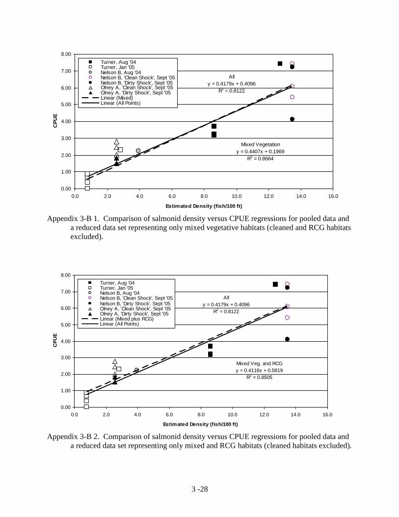
Mixed Vegetation

y = 0.4407x + 0.1969

R2 = 0.8664

All

y = 0.4179x + 0.4096

R2 = 0.8122

0.00

1.00

2.00

3.00

4.00

5.00

6.00

7.00

8.00

0.0 2.0 4.0 6.0 8.0 10.0 12.0 14.0 16.0

Estimated Density (fish/100 ft)

CP

UE

Turner, Aug '04Turner, Jan '05Nelson B, Aug '04Nelson B, 'Clean Shock', Sept '05Nelson B, 'Dirty Shock', Sept '05Olney A, 'Clean Shock', Sept '05Olney A, 'Dirty Shock', Sept '05Linear (Mixed)Linear (All Points)

Appendix 3-B 1. Comparison of salmonid density versus CPUE regressions for pooled data and

a reduced data set representing only mixed vegetative habitats (cleaned and RCG habitats

excluded).

Mixed Veg. and RCG

y = 0.4116x + 0.5819

R2 = 0.8505

All

y = 0.4179x + 0.4096

R2 = 0.8122

0.00

1.00

2.00

3.00

4.00

5.00

6.00

7.00

8.00

0.0 2.0 4.0 6.0 8.0 10.0 12.0 14.0 16.0


CP

UE

Turner, Aug '04Turner, Jan '05Nelson B, Aug '04Nelson B, 'Clean Shock', Sept '05Nelson B, 'Dirty Shock', Sept '05Olney A, 'Clean Shock', Sept '05Olney A, 'Dirty Shock', Sept '05Linear (Mixed plus RCG)Linear (All Points)


a reduced data set representing only mixed and RCG habitats (cleaned habitats excluded).

3 -29

Mixed Veg. and Cleaned

y = 0.452x - 0.0166

R2 = 0.8393

All

y = 0.4179x + 0.4096

R2 = 0.8122

0.00

1.00

2.00

3.00

4.00

5.00

6.00

7.00

8.00

0.0 2.0 4.0 6.0 8.0 10.0 12.0 14.0 16.0


CP

UE

Turner, Aug '04Turner, Jan '05Nelson B, Aug '04Nelson B, 'Clean Shock', Sept '05Nelson B, 'Dirty Shock', Sept '05Olney A, 'Clean Shock', Sept '05Olney A, 'Dirty Shock', Sept '05Linear (Mixed plus Cleaned)Linear (All Points)


a reduced data set representing only mixed and cleaned habitats (RCG habitats excluded).

All Data (non-averaged)

y = 0.4179x + 0.4096

R2 = 0.8122

Site Averaged Data

y = 0.3951x + 0.4414

R2 = 0.923

0.00

1.00

2.00

3.00

4.00

5.00

6.00

7.00

8.00

0.0 2.0 4.0 6.0 8.0 10.0 12.0 14.0 16.0


CP

UE

(S

alm

on

ids/1

00 s

ho

ck s

eco

nd

s)

Turner, Aug '04Turner, Jan '05Nelson B, Aug '04Nelson B, 'Clean Shock', Sept '05Nelson B, 'Dirty Shock', Sept '05Olney A, 'Clean Shock', Sept '05Olney A, 'Dirty Shock', Sept '05Olney C (dredged), Sept '05Site Averaged DataLinear (Best Fit - All Data)Linear (Site Averaged Data)


site-averaged data sets.

drainage salmonid study - king county, washington

Documents