draft - vrije universiteit brusseltinf2.vub.ac.be/~dvermeir/courses/compilers/compilers.pdf · a...
TRANSCRIPT

An introduction to compilersDRAFT
D. VermeirDept. of Computer Science
Vrij Universiteit Brussel, [email protected]
SREVINU
ITEIT
EJIR
V
BRUSSE
L
ECNIVRE TENE
BR
AS
AI
TN
EIC
S
February 4, 2009

Contents
1 Introduction 6
1.1 Compilers and languages . . . . . . . . . . . . . . . . . . . . . . 6
1.2 Applications of compilers . . . . . . . . . . . . . . . . . . . . . . 7
1.3 Overview of the compilation process . . . . . . . . . . . . . . . . 9
1.3.1 Micro . . . . . . . . . . . . . . . . . . . . . . . . . . . . 9
1.3.2 x86 code . . . . . . . . . . . . . . . . . . . . . . . . . . 10
1.3.3 Lexical analysis . . . . . . . . . . . . . . . . . . . . . . . 12
1.3.4 Syntax analysis . . . . . . . . . . . . . . . . . . . . . . . 13
1.3.5 Semantic analysis . . . . . . . . . . . . . . . . . . . . . . 14
1.3.6 Intermediate code generation . . . . . . . . . . . . . . . . 15
1.3.7 Optimization . . . . . . . . . . . . . . . . . . . . . . . . 16
1.3.8 Code generation . . . . . . . . . . . . . . . . . . . . . . 17
2 Lexical analysis 18
2.1 Introduction . . . . . . . . . . . . . . . . . . . . . . . . . . . . . 18
2.2 Regular expressions . . . . . . . . . . . . . . . . . . . . . . . . . 24
2.3 Finite state automata . . . . . . . . . . . . . . . . . . . . . . . . 26
2.3.1 Deterministic finite automata . . . . . . . . . . . . . . . . 26
2.3.2 Nondeterministic finite automata . . . . . . . . . . . . . . 28
2.4 Regular expressions vs finite state automata . . . . . . . . . . . . 31
2.5 A scanner generator . . . . . . . . . . . . . . . . . . . . . . . . . 32
1

VUB-DINF/2009/2 2
3 Parsing 35
3.1 Context-free grammars . . . . . . . . . . . . . . . . . . . . . . . 35
3.2 Top-down parsing . . . . . . . . . . . . . . . . . . . . . . . . . . 38
3.2.1 Introduction . . . . . . . . . . . . . . . . . . . . . . . . . 38
3.2.2 Eliminating left recursion in a grammar . . . . . . . . . . 41
3.2.3 Avoiding backtracking: LL(1) grammars . . . . . . . . . 43
3.2.4 Predictive parsers . . . . . . . . . . . . . . . . . . . . . . 44
3.2.5 Construction of first and follow . . . . . . . . . . . . . . 48
3.3 Bottom-up parsing . . . . . . . . . . . . . . . . . . . . . . . . . 50
3.3.1 Shift-reduce parsers . . . . . . . . . . . . . . . . . . . . 50
3.3.2 LR(1) parsing . . . . . . . . . . . . . . . . . . . . . . . . 54
3.3.3 LALR parsers and yacc/bison . . . . . . . . . . . . . . . 62
4 Checking static semantics 65
4.1 Attribute grammars and syntax-directed translation . . . . . . . . 65
4.2 Symbol tables . . . . . . . . . . . . . . . . . . . . . . . . . . . . 68
4.2.1 String pool . . . . . . . . . . . . . . . . . . . . . . . . . 69
4.2.2 Symbol tables and scope rules . . . . . . . . . . . . . . . 69
4.3 Type checking . . . . . . . . . . . . . . . . . . . . . . . . . . . . 71
5 Intermediate code generation 74
5.1 Postfix notation . . . . . . . . . . . . . . . . . . . . . . . . . . . 75
5.2 Abstract syntax trees . . . . . . . . . . . . . . . . . . . . . . . . 76
5.3 Three-address code . . . . . . . . . . . . . . . . . . . . . . . . . 78
5.4 Translating assignment statements . . . . . . . . . . . . . . . . . 79
5.5 Translating boolean expressions . . . . . . . . . . . . . . . . . . 81
5.6 Translating control flow statements . . . . . . . . . . . . . . . . . 85
5.7 Translating procedure calls . . . . . . . . . . . . . . . . . . . . . 86
5.8 Translating array references . . . . . . . . . . . . . . . . . . . . . 88

VUB-DINF/2009/2 3
6 Optimization of intermediate code 92
6.1 Introduction . . . . . . . . . . . . . . . . . . . . . . . . . . . . . 92
6.2 Local optimization of basic blocks . . . . . . . . . . . . . . . . . 94
6.2.1 DAG representation of basic blocks . . . . . . . . . . . . 95
6.2.2 Code simplification . . . . . . . . . . . . . . . . . . . . . 99
6.2.3 Array and pointer assignments . . . . . . . . . . . . . . . 100
6.2.4 Algebraic identities . . . . . . . . . . . . . . . . . . . . . 101
6.3 Global flow graph information . . . . . . . . . . . . . . . . . . . 101
6.3.1 Reaching definitions . . . . . . . . . . . . . . . . . . . . 103
6.3.2 Reaching definitions using datalog . . . . . . . . . . . . . 105
6.3.3 Available expressions . . . . . . . . . . . . . . . . . . . . 106
6.3.4 Available expressions using datalog . . . . . . . . . . . . 109
6.3.5 Live variable analysis . . . . . . . . . . . . . . . . . . . . 110
6.3.6 Definition-use chaining . . . . . . . . . . . . . . . . . . . 112
6.3.7 Application: uninitialized variables . . . . . . . . . . . . 113
6.4 Global optimization . . . . . . . . . . . . . . . . . . . . . . . . . 113
6.4.1 Elimination of global common subexpressions . . . . . . 113
6.4.2 Copy propagation . . . . . . . . . . . . . . . . . . . . . . 114
6.4.3 Constant folding and elimination of useless variables . . . 116
6.4.4 Loops . . . . . . . . . . . . . . . . . . . . . . . . . . . . 116
6.4.5 Moving loop invariants . . . . . . . . . . . . . . . . . . . 120
6.4.6 Loop induction variables . . . . . . . . . . . . . . . . . . 123
6.5 Aliasing: pointers and procedure calls . . . . . . . . . . . . . . . 126
6.5.1 Pointers . . . . . . . . . . . . . . . . . . . . . . . . . . . 128
6.5.2 Procedures . . . . . . . . . . . . . . . . . . . . . . . . . 128
7 Code generation 130
7.1 Run-time storage management . . . . . . . . . . . . . . . . . . . 131
7.1.1 Global data . . . . . . . . . . . . . . . . . . . . . . . . . 131
7.1.2 Stack-based local data . . . . . . . . . . . . . . . . . . . 132
7.2 Instruction selection . . . . . . . . . . . . . . . . . . . . . . . . . 134

VUB-DINF/2009/2 4
7.3 Register allocation . . . . . . . . . . . . . . . . . . . . . . . . . 136
7.4 Peephole optimization . . . . . . . . . . . . . . . . . . . . . . . 137
A A Short Introduction to x86 Assembler Programming under Linux 139
A.1 Architecture . . . . . . . . . . . . . . . . . . . . . . . . . . . . . 139
A.2 Instructions . . . . . . . . . . . . . . . . . . . . . . . . . . . . . 140
A.2.1 Operands . . . . . . . . . . . . . . . . . . . . . . . . . . 140
A.2.2 Addressing Modes . . . . . . . . . . . . . . . . . . . . . 140
A.2.3 Moving Data . . . . . . . . . . . . . . . . . . . . . . . . 141
A.2.4 Integer Arithmetic . . . . . . . . . . . . . . . . . . . . . 142
A.2.5 Logical Operations . . . . . . . . . . . . . . . . . . . . . 142
A.2.6 Control Flow Instructions . . . . . . . . . . . . . . . . . 142
A.3 Assembler Directives . . . . . . . . . . . . . . . . . . . . . . . . 143
A.4 Calling a function . . . . . . . . . . . . . . . . . . . . . . . . . . 144
A.5 System calls . . . . . . . . . . . . . . . . . . . . . . . . . . . . . 144
A.6 Example . . . . . . . . . . . . . . . . . . . . . . . . . . . . . . . 146
B Mc: the Micro-x86 Compiler 149
B.1 Lexical analyzer . . . . . . . . . . . . . . . . . . . . . . . . . . . 149
B.2 Symbol table management . . . . . . . . . . . . . . . . . . . . . 151
B.3 Parser . . . . . . . . . . . . . . . . . . . . . . . . . . . . . . . . 152
B.4 Driver script . . . . . . . . . . . . . . . . . . . . . . . . . . . . . 155
B.5 Makefile . . . . . . . . . . . . . . . . . . . . . . . . . . . . . . . 156
B.6 Example . . . . . . . . . . . . . . . . . . . . . . . . . . . . . . . 157
B.6.1 Source program . . . . . . . . . . . . . . . . . . . . . . . 157
B.6.2 Assembly language program . . . . . . . . . . . . . . . . 157
C Minic parser and type checker 159
C.1 Lexical analyzer . . . . . . . . . . . . . . . . . . . . . . . . . . . 159
C.2 String pool management . . . . . . . . . . . . . . . . . . . . . . 161
C.3 Symbol table management . . . . . . . . . . . . . . . . . . . . . 163

VUB-DINF/2009/2 5
C.4 Types library . . . . . . . . . . . . . . . . . . . . . . . . . . . . 166
C.5 Type checking routines . . . . . . . . . . . . . . . . . . . . . . . 172
C.6 Parser with semantic actions . . . . . . . . . . . . . . . . . . . . 175
C.7 Utilities . . . . . . . . . . . . . . . . . . . . . . . . . . . . . . . 178
C.8 Driver script . . . . . . . . . . . . . . . . . . . . . . . . . . . . . 179
C.9 Makefile . . . . . . . . . . . . . . . . . . . . . . . . . . . . . . . 180
Index 181
Bibliography 186

Chapter 1
Introduction
1.1 Compilers and languages
A compiler is a program that translates a source language text into an equivalenttarget language text.
E.g. for a C compiler, the source language is C while the target language may beSparc assembly language.
Of course, one expects a compiler to do a faithful translation, i.e. the meaning ofthe translated text should be the same as the meaning of the source text.
One would not be pleased to see the C program in Figure 1.1
1 #include <stdio.h>23 int4 main(int,char**)5 {6 int x = 34;7 x = x*24;8 printf("%d\n",x);9 }
Figure 1.1: A source text in the C language
translated to an assembler program that, when executed, printed “Goodbye world”on the standard output.
So we want the translation performed by a compiler to be semantics preserving.This implies that the compiler is able to “understand” (compute the semantics of)
6

VUB-DINF/2009/2 7
the source text. The compiler must also “understand” the target language in orderto be able to generate a semantically equivalent target text.
Thus, in order to develop a compiler, we need a precise definition of both thesource and the target language. This means that both source and target languagemust be formal.
A language has two aspects: a syntax and a semantics. The syntax prescribeswhich texts are grammatically correct and the semantics specifies how to derivethe meaning from a syntactically correct text. For the C language, the syntaxspecifies e.g. that
“the body of a function must be enclosed between matching braces (“{}”)”.
The semantics says that the meaning of the second statement in Figure 1.1 is that
“the value of the variable x is multiplied by 24 and the result becomesthe new value of the variable x”
It turns out that there exist excellent formalisms and tools to describe the syntaxof a formal language. For the description of the semantics, the situation is lessclear in that existing semantics specification formalisms are not nearly as simpleand easy to use as syntax specifications.
1.2 Applications of compilers
Traditionally, a compiler is thought of as translating a so-called “high level lan-guage” such as C1 or Modula2 into assembly language. Since assembly languagecannot be directly executed, a further translation between assembly language and(relocatable) machine language is necessary. Such programs are usually calledassemblers but it is clear that an assembler is just a special (easier) case of a com-piler.
Sometimes, a compiler translates between high level languages. E.g. the first C++implementations used a compiler called “cfront” which translated C++ code to Ccode. Such a compiler is often called a “cross-compiler”.
On the other hand, a compiler need not target a real assembly (or machine) lan-guage. E.g. Java compilers generate code for a virtual machine called the “Java
1If you want to call C a high-level language

VUB-DINF/2009/2 8
Virtual Machine” (JVM). The JVM interpreter then interprets JVM instructionswithout any further translation.
In general, an interpreter needs to understand only the source language. Insteadof translating the source text, an interpreter immediately executes the instructionsin the source text. Many languages are usually “interpreted”, either directly, orafter a compilation to some virtual machine code: Lisp, Smalltalk, Prolog, SQLare among those. The advantages of using an interpreter are that is easy to porta language to a new machine: all one has to do is to implement the virtual ma-chine on the new hardware. Also, since instructions are evaluated and examinedat run-time, it becomes possible to implement very flexible languages. E.g. for aninterpreter it is not a problem to support variables that have a dynamic type, some-thing which is hard to do in a traditional compiler. Interpreters can even construct“programs” at run time and interpret those without difficulties, a capability that isavailable e.g. for Lisp or Prolog.
Finally, compilers (and interpreters) have wider applications than just translatingprogramming languages. Conceivably any large and complex application mightdefine its own “command language” which can be translated to a virtual machineassociated with the application. Using compiler generating tools, defining andimplementing such a language need not be difficult. Hence SQL can be regardedas such a language associated with a database management system. Other so-called “little languages” provide a convenient interface to specialized libraries.E.g. the language (n)awk is a language that is very convenient to do powerfulpattern matching and extraction operations on large text files.

VUB-DINF/2009/2 9
1.3 Overview of the compilation process
In this section we will illustrate the main phases of the compilation process througha simple compiler for a toy programming language. The source for an implemen-tation of this compiler can be found in Appendix B and on the web site of thecourse.
program : declaration list statement list;
declaration list : declaration ; declaration list| ε;
declaration : declare var;
statement list : statement ; statement list| ε;
statement : assignment| read statement| write statement;
assignment : var = expression;
read statement : read var;
write statement : write expression;
expression : term| term + term| term − term;
term : NUMBER| var| ( expression );
var : NAME;
Figure 1.2: The syntax of the Micro language
1.3.1 Micro
The source language “Micro” is very simple. It is based on the toy languagedescribed in [FL91].

VUB-DINF/2009/2 10
The syntax of Micro is described by the rules in Figure 1.2. We will see in Chap-ter 3 that such rules can be formalized into what is called a grammar.
Note that NUMBER and NAME have not been further defined. The idea is, ofcourse, that NUMBER represents a sequence of digits and that NAME representsa string of letters and digits, starting with a letter.
A simple Micro program is shown in Figure 1.3
{declare xyz;xyz = (33+3)-35;write xyz;}
Figure 1.3: A Micro program
The semantics of Micro should be clear2: a Micro program consists of a sequenceof read/write or assignment statements. There are integer-valued variables (whichneed to be declared before they are used) and expressions are restricted to additionand substraction.
1.3.2 x86 code
The target language will be code for the x86 processor family. Figure 1.4 showspart of the output of the compiler for the program of Figure 1.3. The full outputcan be found in Section B.6.2, page 157.
X86 processors have a number of registers, some of which are special purpose,such as the esp register which always points to the top of the stack (which growsdownwards). More information on x86 assembler programming can be found inthe Appendix, Section A, page 139.
line 1 The code is divided into data and text sections where the latter contains theactual instructions.
line 2 This defines a data area of 4 bytes wide which can be referenced using thename xyz. This definition is the translation of a Micro declaration.
2The output of the program in Figure 1.3 is, of course, 1.

VUB-DINF/2009/2 11
1 .section .data2 .lcomm xyz, 43 .section .text
...44 .globl main45 .type main, @function46 main:47 pushl %ebp48 movl %esp, %ebp49 pushl $3350 pushl $351 popl %eax52 addl %eax, (%esp)53 pushl $3554 popl %eax55 subl %eax, (%esp)56 popl xyz57 pushl xyz58 call print59 movl %ebp, %esp60 popl %ebp61 ret
...
Figure 1.4: X86 assembly code generated for the program in Figure 1.3
line 44 This defines main as a globally available name. It will be used to referto the single function (line 45) that contains the instructions correspondingto the Micro program. The function starts at line 46 where the locationcorresponding to the label ’main’ is defined.
line 47 Together with line 48, this starts off the function according to the C call-ing conventions: the current top of stack contains the return address. Thisaddress has been pushed on the stack by the (function) call instruction.It will eventually be used (and popped) by a subsequent ret (return fromfunction call) instruction. Parameters are passed by pushing them on thestack just before the call instruction. Line 47 saves the caller’s “basepointer” in the ebp register by pushing it on the stack before setting (line 48)the current top of the stack as a new base pointer ebp. When returning fromthe function call, the orginal stack is restored by copying the saved valuefrom ebp to esp (line 59) and popping the saved base pointer (line 60).
line 49 The evaluation of the subexpression 33 + 3 is initiated by pushing bothconstants (indicates by the use of a ’$’ prefix) on the stack (lines 49, 50)

VUB-DINF/2009/2 12
line 51 Once both operands are on the top of the stack, the operation (correspondingto the 33 + 3 expression) is executed by popping the second argument to theeax register (line 51) which is then added to the first argument on the top ofthe stack (line 52). The net result is that the two arguments of the operationare replaced on the top of the stack by the (single) result of the operation.
line 53 To substract 35 from the result, this second argument of the substraction ispushed on the stack (line 53), after which the substraction is executed onthe two operands on the stack, replacing them on the top of the stack by theresult (lines 54,55).
line 56 The result of evaluating the expression is assigned to the variable xyz bypopping it from the stack to the appropriate address.
line 57 In order to print the value at address xyz, it is first pushed on the stack asa parameter for a subsequent call (line 58) to a print function (the code ofwhich can be found in Section B.6.2).
1.3.3 Lexical analysis
The raw input to a compiler consists of a string of bytes or characters. Someof those characters, e.g. the “{” character in Micro, may have a meaning bythemselves. Other characters only have meaning as part of a larger unit. E.g. the“y” in the example program from Figure 1.3, is just a part of the NAME “xyz”.Still others, such as “ ”, “\n” serve as separators to distinguish one meaningfulstring from another.
The first job of a compiler is then to group sequences of raw characters into mean-ingful tokens. The lexical analyzer module is responsible for this. Conceptually,the lexical analyzer (often called scanner) transforms a sequence of charactersinto a sequence of tokens. In addition, a lexical analyzer will typically accessthe symbol table to store and/or retrieve information on certain source languageconcepts such as variables, functions, types.
For the example program from Figure 1.3, the lexical analyzer will transform thecharacter sequence
{ declare xyz; xyz = (33+3)-35; write xyz; }
into the token sequence shown in Figure 1.5.
Note that some tokens have “properties”, e.g. a 〈NUMBER〉 token has a valueproperty while a 〈NAME〉 token has a symbol table reference as a property.

VUB-DINF/2009/2 13
〈LBRACE〉〈DECLARE symbol table ref=0〉〈NAME symbol table ref=3〉〈SEMICOLON〉〈NAME symbol table ref=3〉〈ASSIGN〉〈LPAREN〉〈NUMBER value=33〉〈PLUS〉〈NUMBER value=3〉〈RPAREN〉〈MINUS〉〈NUMBER value=35〉〈SEMICOLON〉〈WRITE symbol table ref=2〉〈NAME symbol table ref=3〉〈SEMICOLON〉〈RBRACE〉
Figure 1.5: Result of lexical analysis of program in Figure 1.3
After the scanner finishes, the symbol table in the example could look like
0 “declare” DECLARE1 “read” READ2 “write” WRITE3 “xyz” NAME
where the third column indicates the type of symbol.
Clearly, the main difficulty in writing a lexical analyzer will be to decide, whilereading characters one by one, when a token of which type is finished. We willsee in Chapter 2 that regular expressions and finite automata provide a powerfuland convenient method to automate this job.
1.3.4 Syntax analysis
Once lexical analysis is finished, the parser takes over to check whether the se-quence of tokens is grammatically correct, according to the rules that define thesyntax of the source language.
Looking at the grammar rules for Micro (Figure 1.2), it seems clear that a programis syntactically correct if the structure of the tokens matches the structure of a〈program〉 as defined by these rules.

VUB-DINF/2009/2 14
Such matching can conveniently be represented as a parse tree. The parse treecorresponding to the token sequence of Figure 1.5 is shown in Figure 1.6.
<program>
<statement> <statement_list>
<statement>
<RBRACE}
<SEMICOLON>
<SEMICOLON><LBRACE>
<statement_list>
<assignment>
<expression>
<term> <term>
<expression>
<term>
(xyz)
<term>
(33) (3)
(35)
<NAME> <ASSIGN>
<MINUS>
<LPAREN> <RPAREN> <NUMBER>
<NUMBER>
<PLUS>
<NUMBER>
<statement> <SEMICOLON>
<write_statement>
<expression>
<term>
<var>
(xyz)
<NAME>
<WRITE>
<declaration>
(xyz)
<DECLARE> <NAME>
<statement_list>
<>
Figure 1.6: Parse tree of program in Figure 1.3
Note that in the parse tree, a node and its children correspond to a rule in thesyntax specification of Micro: the parent node corresponds to the left hand sideof the rule while the children correspond to the right hand side. Furthermore, theyield3 of the parse tree is exactly the sequence of tokens that resulted from thelexical analysis of the source text.
Hence the job of the parser is to construct a parse tree that fits, according to thesyntax specification, the token sequence that was generated by the lexical ana-lyzer.
In Chapter 3, we’ll see how context-free grammars can be used to specify thesyntax of a programming language and how it is possible to automatically generateparser programs from such a context-free grammar.
1.3.5 Semantic analysis
Having established that the source text is syntactically correct, the compiler maynow perform additional checks such as determining the type of expressions and
3The yield of a tree is the sequence of leafs of the tree in lexicographical (left-to-right) order

VUB-DINF/2009/2 15
checking that all statements are correct with respect to the typing rules, that vari-ables have been properly declared before they are used, that functions are calledwith the proper number of parameters etc.
This phase is carried out using information from the parse tree and the symbol ta-ble. In our example, very little needs to be checked, due to the extreme simplicityof the language. The only check that is performed verifies that a variable has beendeclared before it is used.
1.3.6 Intermediate code generation
In this phase, the compiler translates the source text into an simple intermediatelanguage. There are several possible choices for an intermediate language. butin this example we will use the popular “three-address code” format. Essentially,three-address code consists of assignments where the right-hand side must be asingle variable or constant or the result of a binary or unary operation. Hencean assignment involves at most three variables (addresses), which explains thename. In addition, three-address code supports primitive control flow statementssuch as goto, branch-if-positive etc. Finally, retrieval from and storing into a one-dimensional array is also possible.
The translation process is syntax-directed. This means that
• Nodes in the parse tree have a set of attributes that contain informationpertaining to that node. The set of attributes of a node depends on thekind of syntactical concept it represents. E.g. in Micro, an attribute of an〈expression〉 could be the sequence of x86 instructions that leave the resultof the evaluation of the expression on the top of the stack. Similarly, both〈var〉 and 〈expression〉 nodes have a name attribute holding the name of thevariable containing the current value of the 〈var〉 or 〈expression〉We use n.a to refer to the value of the attribute a for the node n.
• A number of semantic rules are associated with each syntactic rule of thegrammar. These semantic rules determine the values of the attributes of thenodes in the parse tree (a parent node and its children) that correspond tosuch a syntactic rule. E.g. in Micro, there is a semantic rule that says thatthe code associated with an 〈assignment〉 in the rule
assignment : var = expression

VUB-DINF/2009/2 16
consists of the code associated with 〈expression〉 followed by a three-addresscode statement of the form
var.name = expression.name
More formally, such a semantic rule might be written as
assignment.code = expression.code ‖ “var.name = expression.name”
• The translation of the source text then consists of the value of a particularattribute for the root of the parse tree.
Thus intermediate code generation can be performed by computing, using thesemantic rules, the attribute values of all nodes in the parse tree. The result is thenthe value of a specific (e.g. “code”) attribute of the root of the parse tree.
For the example program from Figure 1.3, we could obtain the three-address codein Figure 1.7.
T0 = 33 +3T1 = T0 - 35XYZ = T1WRITE XYZ
Figure 1.7: three-address code corresponding to the program of Figure 1.3
Note the introduction of several temporary variables, due to the restrictions in-herent in three-address code. The last statement before the WRITE may seemwasteful but this sort of inefficiency is easily taken care of by the next optimiza-tion phase.
1.3.7 Optimization
In this phase, the compiler tries several optimization methods to replace fragmentsof the intermediate code text with equivalent but faster (and usually also shorter)fragments.
Techniques that can be employed include common subexpression elimination,loop invariant motion, constant folding etc. Most of these techniques need ex-tra information such as a flow graph, live variable status etc.
In our example, the compiler could perform constant folding and code reorderingresulting in the optimized code of Figure 1.8.

VUB-DINF/2009/2 17
XYZ = 1WRITE XYZ
Figure 1.8: Optimized three-address code corresponding to the program of Fig-ure 1.3
1.3.8 Code generation
The final phase of the compilation consists of the generation of target code fromthe intermediate code. When the target code corresponds to a register machine, amajor problem is the efficient allocation of scarce but fast registers to variables.This problem may be compared with the paging strategy employed by virtualmemory management systems. The goal is in both cases to minimize traffic be-tween fast (the registers for a compiler, the page frames for an operating system)and slow (the addresses of variables for a compiler, the pages on disk for an op-erating system) memory. A significant difference between the two problems isthat a compiler has more (but not perfect) knowledge about future references tovariables, so more optimization opportunities exist.

Chapter 2
Lexical analysis
2.1 Introduction
As seen in Chapter 1, the lexical analyzer must transform a sequence of “raw”characters into a sequence of tokens. Often a token has a structure as in Figure 2.1.
1 #ifndef LEX_H2 #define LEX_H3 // %M%(%I%) %U% %E%45 typedef enum { NAME, NUMBER, LBRACE, RBRACE, LPAREN, RPAREN, ASSIGN,6 SEMICOLON, PLUS, MINUS, ERROR } TOKENT;78 typedef struct9 {
10 TOKENT type;11 union {12 int value; /* type == NUMBER */13 char *name; /* type == NAME */14 } info;15 } TOKEN;1617 extern TOKEN *lex();18 #endif LEX_H
Figure 2.1: A declaration for TOKEN and lex()
Actually, the above declaration is not realistic. Usually, more “complex” tokenssuch as NAMEs will refer to a symbol table entry rather than simply their stringrepresentation.
18
VUB-DINF/2009/2 19
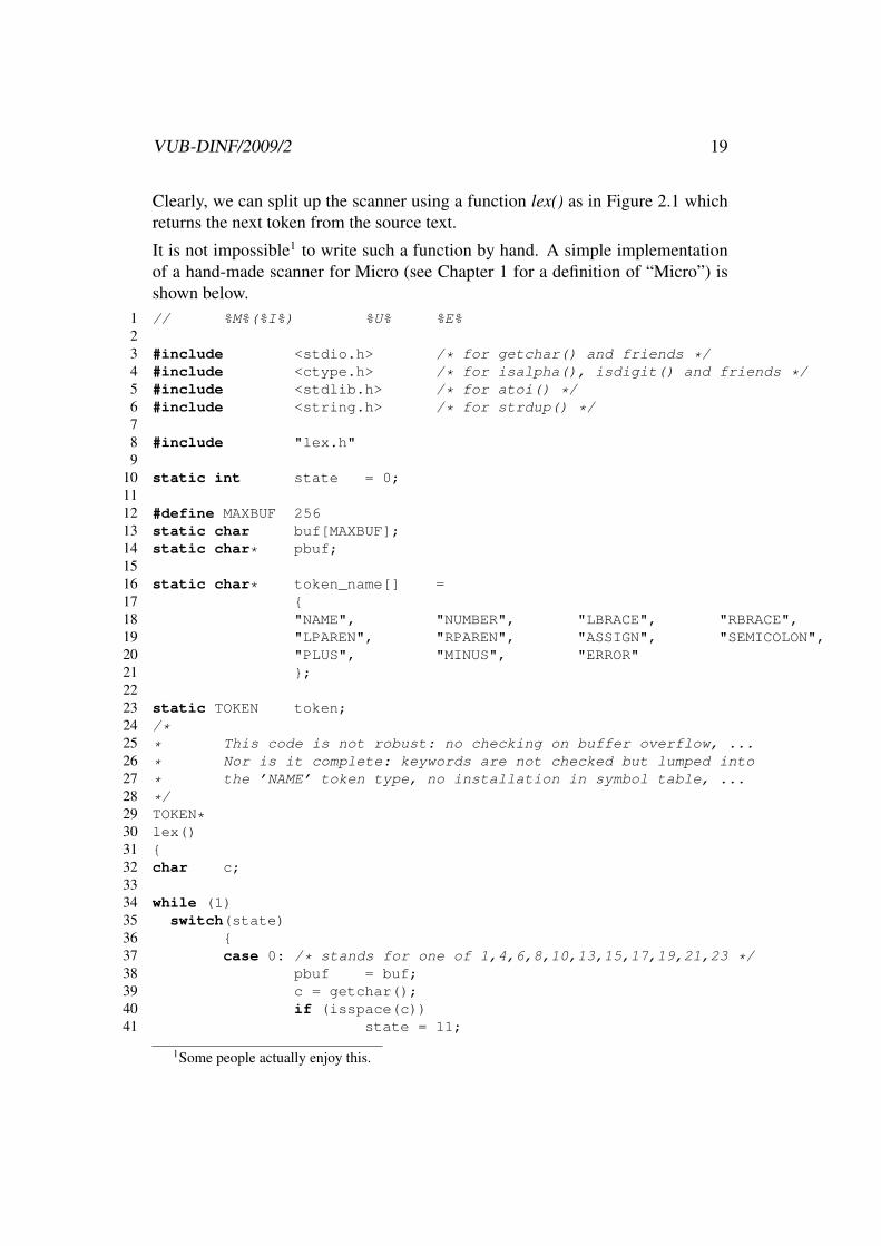
Clearly, we can split up the scanner using a function lex() as in Figure 2.1 whichreturns the next token from the source text.
It is not impossible1 to write such a function by hand. A simple implementationof a hand-made scanner for Micro (see Chapter 1 for a definition of “Micro”) isshown below.
1 // %M%(%I%) %U% %E%23 #include <stdio.h> /* for getchar() and friends */4 #include <ctype.h> /* for isalpha(), isdigit() and friends */5 #include <stdlib.h> /* for atoi() */6 #include <string.h> /* for strdup() */78 #include "lex.h"9
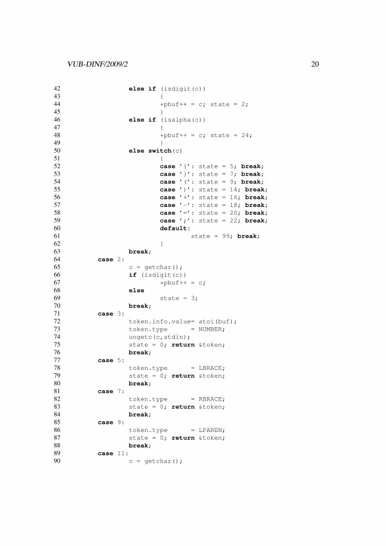
10 static int state = 0;1112 #define MAXBUF 25613 static char buf[MAXBUF];14 static char* pbuf;1516 static char* token_name[] =17 {18 "NAME", "NUMBER", "LBRACE", "RBRACE",19 "LPAREN", "RPAREN", "ASSIGN", "SEMICOLON",20 "PLUS", "MINUS", "ERROR"21 };2223 static TOKEN token;24 /*25 * This code is not robust: no checking on buffer overflow, ...26 * Nor is it complete: keywords are not checked but lumped into27 * the ’NAME’ token type, no installation in symbol table, ...28 */29 TOKEN*30 lex()31 {32 char c;3334 while (1)35 switch(state)36 {37 case 0: /* stands for one of 1,4,6,8,10,13,15,17,19,21,23 */38 pbuf = buf;39 c = getchar();40 if (isspace(c))41 state = 11;
1Some people actually enjoy this.
VUB-DINF/2009/2 20
42 else if (isdigit(c))43 {44 *pbuf++ = c; state = 2;45 }46 else if (isalpha(c))47 {48 *pbuf++ = c; state = 24;49 }50 else switch(c)51 {52 case ’{’: state = 5; break;53 case ’}’: state = 7; break;54 case ’(’: state = 9; break;55 case ’)’: state = 14; break;56 case ’+’: state = 16; break;57 case ’-’: state = 18; break;58 case ’=’: state = 20; break;59 case ’;’: state = 22; break;60 default:61 state = 99; break;62 }63 break;64 case 2:65 c = getchar();66 if (isdigit(c))67 *pbuf++ = c;68 else69 state = 3;70 break;71 case 3:72 token.info.value= atoi(buf);73 token.type = NUMBER;74 ungetc(c,stdin);75 state = 0; return &token;76 break;77 case 5:78 token.type = LBRACE;79 state = 0; return &token;80 break;81 case 7:82 token.type = RBRACE;83 state = 0; return &token;84 break;85 case 9:86 token.type = LPAREN;87 state = 0; return &token;88 break;89 case 11:90 c = getchar();

VUB-DINF/2009/2 21
91 if (isspace(c))92 ;93 else94 state = 12;95 break;96 case 12:97 ungetc(c,stdin);98 state = 0;99 break;
100 case 14:101 token.type = RPAREN;102 state = 0; return &token;103 break;104 case 16:105 token.type = PLUS;106 state = 0; return &token;107 break;108 case 18:109 token.type = MINUS;110 state = 0; return &token;111 break;112 case 20:113 token.type = ASSIGN;114 state = 0; return &token;115 break;116 case 22:117 token.type = SEMICOLON;118 state = 0; return &token;119 break;120 case 24:121 c = getchar();122 if (isalpha(c)||isdigit(c))123 *pbuf++ = c;124 else125 state = 25;126 break;127 case 25:128 *pbuf = (char)0;129 token.info.name = strdup(buf);130 token.type = NAME;131 ungetc(c,stdin);132 state = 0; return &token;133 break;134 case 99:135 if (c==EOF)136 return 0;137 fprintf(stderr,"Illegal character: \’%c\’\n",c);138 token.type = ERROR;139 state = 0; return &token;

VUB-DINF/2009/2 22
140 break;141 default:142 break; /* Cannot happen */143 }144 }145146 int147 main()148 {149 TOKEN *t;150151 while ((t=lex()))152 {153 printf("%s",token_name[t->type]);154 switch (t->type)155 {156 case NAME:157 printf(": %s\n",t->info.name);158 break;159 case NUMBER:160 printf(": %d\n",t->info.value);161 break;162 default:163 printf("\n");164 break;165 }166 }167 return 0;168 }
The control flow in the above lex() procedure can be represented by a combinationof so-called transition diagrams which are shown in Figure 2.2.
There is a transition diagram for each token type and another one for white space(blank, tab, newline). The code for lex() simply implements those diagrams. Theonly complications are
• When starting a new token (i.e., upon entry to lex()), we use a “special”state 0 to represent the fact that we didn’t decide yet which diagram tofollow. The choice here is made on the basis of the next input character.
• In Figure 2.2, bold circles represent states where we are sure which tokenhas been recognized. Sometimes (e.g. for the LBRACE token type) weknow this immediately after scanning the last character making up the to-ken. However, for other types, like NUMBER, we only know the full extentof the token after reading an extra character that will not belong to the to-

VUB-DINF/2009/2 23
digit not(digit)
digit
letter
letter | digit
not(letter | digit)
*
*
1 2 3
*spnl
spnl
not(spnl)
} (
)
+ − =
;
16
21 22
15 17
10 11 12 13
18
14
19 20
9876{
54
23 24 25
Figure 2.2: The transition diagram for lex()
ken. In such a case we must push the extra character back onto the inputbefore returning. Such states have been marked with a * in Figure 2.2.
• If we read a character that doesn’t fit any transition diagram, we return aspecial ERROR token type.
Clearly, writing a scanner by hand seems to be easy, once you have a set of tran-sition diagrams such as the ones in Figure 2.2. It is however also boring, anderror-prone, especially if there are a large number of states.
Fortunately, the generation of such code can be automated. We will describe howa specification of the various token types can be automatically converted in codethat implements a scanner for such token types.
First we will design a suitable formalism to specify token types.

VUB-DINF/2009/2 24
2.2 Regular expressions
In Micro, a NUMBER token represents a digit followed by 0 or more digits. ANAME consists of a letter followed by 0 or more alphanumeric characters. ALBRACE token consists of exactly one “{” character, etc.
Such specifications are easily formalized using regular expressions. Before defin-ing regular expressions we should recall the notion of alphabet (a finite set ofabstract symbols, e.g. ASCII characters), and (formal) language (a set of stringscontaining symbols from some alphabet).
The length of a string w, denoted |w| is defined as the number of symbols occur-ring in w. The prefix of length l of a string w, denoted pref l(w) is defined as thelongest string x such that |x| ≤ l and w = xy for some string y. The empty string(of length 0) is denoted ε. The product L1.L2 of two languages is the language
L1.L2 = {xy | x ∈ L1 ∧ y ∈ L2}
The closure L∗ of a language L is defined by
L∗ = ∪i∈NLi
(where, of course, L0 = {ε} and Li+1 = L.Li).
Definition 1 The following table, where r and s denote arbitrary regular expres-sions, recursively defines all regular expressions over a given alphabet Σ, togetherwith the language Lx each expression x represents.
Regular expression Language∅ ∅ε {ε}a {a}(r + s) Lr ∪ Ls(rs) Lr · Ls(r∗) L∗r
In the table, r and s denote arbitrary regular expressions, and a ∈ Σ is an arbi-trary symbol from Σ.
A language L for which there exists a regular r expression such that Lr = L iscalled a regular language.

VUB-DINF/2009/2 25
We assume that the operators +, concatenation and ∗ have increasing precedence,allowing us to drop many parentheses without risking confusion. Thus, ((0(1∗)) + 0)may be written as 01∗ + 0.
From Figure 2.2 we can deduce regular expressions for each token type, as shownin Figure 2.1. We assume that
Σ = {a, . . . , z, A, . . . , Z, 0, . . . , 9,SP,NL, (, ),+,=, {, }, ; ,−}
Token type or abbreviation Regular expressionletter a+ . . .+ z + A+ . . .+ Zdigit 0 + 1 + 2 + 3 + 4 + 5 + 6 + 7 + 8 + 9NUMBER digit(digit)∗
NAME letter(letter + digit)∗
space (SP + NL)(SP + NL)∗
LBRACE {.. ..
Table 2.1: Regular expressions describing Micro tokens
A full specification, such as the one in Section B.1, page 149, then consists of aset of (extended) regular expressions, plus C code for each expression. The ideais that the generated scanner will
• Process input characters, trying to find a longest string that matches any ofthe regular expressions2.
• Execute the code associated with the selected regular expression. This codecan, e.g. install something in the symbol table, return a token type or what-ever.
In the next section we will see how a regular expression can be converted to a so-called deterministic finite automaton that can be regarded as an abstract machineto recognize strings described by regular expressions. Automatic translation ofsuch an automaton to actual code will turn out to be straightforward.
2If two expressions match the same longest string, the one that was declared first is chosen.

VUB-DINF/2009/2 26
2.3 Finite state automata
2.3.1 Deterministic finite automata
Definition 2 A deterministic finite automaton (DFA) is a tuple
(Q,Σ, δ, q0, F )
where
• Q is a finite set of states,
• Σ is a finite input alphabet
• δ : Q× Σ→ Q is a (total) transition function
• q0 ∈ Q is the initial state
• F ⊆ Q is the set of final states
Definition 3 Let M = (Q,Σ, δ, q0, F ) be a DFA. A configuration of M is a pair(q, w) ∈ Q× Σ∗. For a configuration (q, aw) (where a ∈ Σ), we write
(q, aw) `M (q′, w)
just when δ(q, a) = q′ 3. The reflexive and transitive closure of the binary relation`M is denoted as `∗M . A sequence
c0 `M c1 `M . . . `M cn
is called a computation of n ≥ 0 steps by M .
The language accepted by M is defined by
L(M) = {w | ∃q ∈ F · (q0, w) `∗M (q, ε)}
We will often write δ∗(q, w) to denote the unique q′ ∈ Q such that (q, w) `∗M(q′, ε).
3We will drop the subscript M in `M if M is clear from the context.

VUB-DINF/2009/2 27
Example 1 Assuming an alphabet Σ = {l, d, o} (where “l” stands for “letter”,“d” stands for “digit” and “o” stands for “other”), a DFA recognizing MicroNAMEs can be defined as follows:
M = ({q0, qe, q1}, {l, d, o}, δ, q0, {q1})
where δ is defined by
δ(q0, l) = q1
δ(q0, d) = qe
δ(q0, o) = qe
δ(q1, l) = q1
δ(q1, d) = q1
δ(q1, o) = qe
δ(qe, l) = qe
δ(qe, d) = qe
δ(qe, o) = qe
M is shown in Figure 2.3 (the initial state has a small incoming arrow, final statesare in bold):
q0 q1
qe
l
l
do
o
d
l
d
o
Figure 2.3: A DFA for NAME
Clearly, a DFA can be efficiently implemented, e.g. by encoding the states asnumbers and using an array to represent the transition function. This is illustratedin Figure 2.4. The next state array can be automatically generated from theDFA description.
What is not clear is how to translate regular expressions to DFA’s. To show howthis can be done, we need the more general concept of a nondeterministic finiteautomaton (NFA).

VUB-DINF/2009/2 28
1 typedef int STATE;2 typedef char SYMBOL;3 typedef enum {false,true} BOOL;45 STATE next_state[SYMBOL][STATE];6 BOOL final[STATE];78 BOOL9 dfa(SYMBOL *input,STATE q)
10 {11 SYMBOl c;1213 while (c=*input++)14 q = next_state[c,q];15 return final[q];16 }
Figure 2.4: DFA implementation
2.3.2 Nondeterministic finite automata
A nondeterministic finite automaton is much like a deterministic one except thatwe now allow several possibilities for a transition on the same symbol from agiven state. The idea is that the automaton can arbitrarily (nondeterministically)choose one of the possibilities. In addition, we will also allow ε-moves where theautomaton makes a state transition (labeled by ε) without reading an input symbol.
Definition 4 A nondeterministic finite automaton (NFA) is a tuple
(Q,Σ, δ, q0, F )
where
• Q is a finite set of states,
• Σ is a finite input alphabet
• δ : Q× (Σ ∪ {ε})→ 2Q is a (total) transition function 4
• q0 ∈ Q is the initial state
• F ⊆ Q is the set of final states

VUB-DINF/2009/2 29
ba
q2
q1q0a
b
Figure 2.5: M1
It should be noted that ∅ ∈ 2Q and thus Definition 4 sanctions the possibility ofthere not being any transition from a state q on a given symbol a.
Example 2 Consider M1 = ({q0, q1, q2}, δ1, q0, {q0}) as depicted in Figure 2.5.The table below defines δ1:
q ∈ Q σ ∈ Σ δ1(q, σ)q0 a {q1}q0 b ∅q1 a ∅q1 b {q0, q2}q2 a {q0}q2 b ∅
The following definition formalizes our intuition about the behavior of nondeter-ministic finite automata.
Definition 5 Let M = (Q,Σ, δ, q0, F ) be a NFA. A configuration of M is a pair(q, w) ∈ Q× Σ∗. For a configuration (q, aw) (where a ∈ Σ ∪ {ε}), we write
(q, aw) `M (q′, w)
just when q′ ∈ δ(q, a) 5. The reflexive and transitive closure of the binary relation`M is denoted as `∗M . The language accepted by M is defined by
L(M) = {w | ∃q ∈ F · (q0, w) `∗M (q, ε)}4For any set X , we use 2X to denote its power set, i.e. the set of all subsets of X .5We will drop the subscript M in `M if M is clear from the context.

VUB-DINF/2009/2 30
Example 3 The following sequence shows how M1 from Example 2 can acceptthe string abaab:
(q0, abaab) `M1 (q1, baab)
`M1 (q2, aab)
`M1 (q0, ab)
`M1 (q1, b)
`M1 (q0, ε)
L(M1) = {w0w1 . . . wn | n ∈ N ∧ ∀0 ≤ i ≤ n · wi ∈ {ab, aba}}
Although nondeterministic finite automata are more general than deterministicones, it turns out that they are not more powerful in the sense that any NFA canbe simulated by a DFA.
Theorem 1 Let M be a NFA. There exists a DFA M ′ such that L(M ′) = L(M).
Proof: (sketch) Let M = (Q,Σ, δ, q0, F ) be a NFA. We will construct a DFA M ′
that simulates M . This is achieved by letting M ′ be “in all possible states” thatM could be in (after reading the same symbols). Note that “all possible states” isalways an element of 2Q, which is finite since Q is.
To deal with ε-moves, we note that, if M is in a state q, it could also be in anystate q′ to which there is an ε-transition from q. This motivates the definition ofthe ε-closure Cε(S) of a set of states S:
Cε(S) = {p ∈ Q | ∃q ∈ S · (q, ε) `∗M (p, ε)} (2.1)
Now we defineM ′ = (2Q,Σ, δ′, s0, F
′)
where
• δ′ is defined by
∀s ∈ 2Q, a ∈ Σ · δ′(s, a) = ∪q∈sCε(δ(q, a)) (2.2)
• s0 = Cε(q0), i.e. M ′ starts in all possible states where M could go to fromq0 without reading any input.
• F ′ = {s ∈ 2Q | s ∩ F 6= ∅}, i.e. if M could end up in a final state, then M ′
will do so.
It can then be shown that L(M ′) = L(M). 2

VUB-DINF/2009/2 31
2.4 Regular expressions vs finite state automata
In this section we show how a regular expression can be translated to a nondeter-ministic finite automata that defines the same language. Using Theorem 1, we canthen translate regular expressions to DFA’s and hence to a program that acceptsexactly the strings conforming to the regular expression.
Theorem 2 Let r be a regular expression. Then there exists a NFA Mr such thatL(Mr) = Lr.
Proof:We show by induction on the number of operators used in a regular expression rthat Lr is accepted by an NFA
Mr = (Q,Σ, δ, q0, {qf})
(where Σ is the alphabet of Lr) which has exactly one final state qf satisfying
∀a ∈ Σ ∪ {ε} · δ(qf , a) = ∅ (2.3)
Base case
Assume that r does not contain any operator. Then r is one of ∅, ε or a ∈ Σ.
We then define M∅, Mε and Ma as shown in Figure 2.6.
aMa
Mε
M∅
Figure 2.6: M∅,Mε and Ma
Induction step
More complex regular expressions must be of one of the forms r1 + r2, r1r2 or r∗1.In each case, we can construct a NFA Mr1+r2 , Mr1r2 or Mr∗1
, based on Mr1 andMr2 , as shown in Figure 2.7.

VUB-DINF/2009/2 32
Mr1∗
Mr1r2
Mr1+r2
Mr1
Mr2
ε
ε ε
ε
q0 qf
q0 qfε ε ε
ε
ε
ε
εMr1
q0 qf
Mr2Mr1
Figure 2.7: Mr1+r2 ,Mr1r2 and Mr∗1
It can then be shown that
L(Mr1+r2) = L(Mr1) ∪ L(Mr2)
L(Mr1r2) = L(Mr1) L(Mr2)
L(Mr∗1) = L(Mr1)
∗
2
2.5 A scanner generator
We can now be more specific on the design and operation of a scanner generatorsuch as lex(1) or flex(1L), which was sketched on page 25.
First we introduce the concept of a “dead” state in a DFA.
Definition 6 Let M = (Q,Σ, δ, q0, F ) be a DFA. A state q ∈ Q is called dead ifthere does not exist a string w ∈ Σ∗ such that (q, w) `∗M (qf , ε) for some qf ∈ F .

VUB-DINF/2009/2 33
Example 4 The state qe in Example 1 is dead.
It is easy to determine the set of dead states for a DFA, e.g. using a markingalgorithm which initially marks all states as “dead” and then recursively worksbackwards from the final states, unmarking any states reached.
The generator takes as input a set of regular expressions,R = {r1, . . . , rn} each ofwhich is associated with some code cri to be executed when a token correspondingto ri is recognized.
The generator will convert the regular expression
r1 + r2 + . . .+ rn
to a DFA M = (Q,Σ, δ, q0, F ), as shown in Section 2.4, with one addition: whenconstructing M , it will remember which final state of the DFA corresponds withwhich regular expression. This can easily be done by remembering the final statesin the NFA’s corresponding to each of the ri while constructing the combined DFAM . It may be that a final state in the DFA corresponds to several patterns (regularexpressions). In this case, we select the one that was defined first.
Thus we have a mappingpattern : F → R
which associates the first (in the order of definition) pattern to which a certain finalstate corresponds. We also compute the set of dead states of M .
The code in Figure 2.8 illustrates the operation of the generated scanner.
The scanner reads input characters, remembering the last final state seen and theassociated regular expression, until it hits a dead state from where it is impossibleto reach a final state. It then backs up to the last final state and executes the codeassociated with that pattern. Clearly, this will find the longest possible token onthe input.

VUB-DINF/2009/2 34
1 typedef int STATE;2 typedef char SYMBOL;3 typedef enum {false,true} BOOL;45 typedef struct { /* what we need to know about a user defined pattern */6 TOKEN* (*code)(); /* user-defined action */7 BOOL do_return; /* whether action returns from lex() or not */8 } PATTERN;9
10 static STATE next_state[SYMBOL][STATE];11 static BOOL dead[STATE];12 static BOOL final[STATE];13 static PATTERN* pattern[STATE]; /* first regexp for this final state */14 static SYMBOL *last_input = 0; /* input pointer at last final state */15 static STATE last_state, q = 0; /* assuming 0 is initial state */16 static SYMBOL *input; /* source text */1718 TOKEN*19 lex()20 {21 SYMBOl c;22 PATTERN *last_pattern = 0;2324 while (c=*input++) {25 q = next_state[c,q];26 if (final[q]) {27 last_pattern = pattern[q];28 last_input = input;29 last_state = q;30 }31 if (dead[q]) {32 if (last_pattern) {33 input = last_input;34 q = 0;35 if (last_pattern->do_return)36 return pattern->code();37 else38 pattern->code();39 }40 else /* error */41 ;42 }43 }4445 return (TOKEN*)0;46 }
Figure 2.8: A generated scanner

Chapter 3
Parsing
3.1 Context-free grammars
As mentioned in Section 1.3.1, page 9, the rules (or railroad diagrams) used tospecify the syntax of a programming language can be formalized using the conceptof context-free grammar.
Definition 7 A context-free grammar (cfg) is a tuple
G = (V,Σ, P, S)
where
• V is a finite set of nonterminal symbols
• Σ is a finite set of terminal symbols, disjoint from V : Σ ∩ V = ∅.
• P is a finite set of productions of the form A → α where A ∈ V andα ∈ (V ∪ Σ)∗
• S ∈ V is a nonterminal start symbol
Note that terminal symbols correspond to token types as delivered by the lexicalanalyzer.
Example 5 The following context-free grammar defines the syntax of simplearithmetic expressions:
G0 = ({E}, {+,×, (, ), id}, P, E)
35

VUB-DINF/2009/2 36
where P consists of
E → E + E
E → E × EE → (E)
E → id
We shall often use a shorter notation for a set of productions where several right-hand sides for the same nonterminal are written together, separated by “|”. Usingthis notation, the set of rules of G0 can be written as
E → E + E | E × E | (E) | id
Definition 8 LetG = (V,Σ, P, S) be a context-free grammar. For strings x, y ∈ (V ∪ Σ)∗,we say that x derives y in one step, denoted x =⇒G y iff x = x1Ax2, y = x1αx2
and A→ α ∈ P . Thus =⇒G is a binary relation on (V ∪ Σ)∗. The relation=⇒∗Gis the reflexive and transitive closure of =⇒G. The language L(G) generated byG is defined by
L(G) = {w ∈ Σ∗ | S =⇒∗G w}A language is called context-free if it is generated by some context-free grammar.A derivation in G of wn from w0 is any sequence of the form
w0 =⇒G w1 =⇒G . . . =⇒G wn
where n ≥ 0 (we say that the derivation has n steps) and ∀1 ≤ i ≤ n · wi ∈ (V ∪ Σ)∗
We write v =⇒nG w (n ≥ 0) when w can be derived from v in n steps.
Thus a context-free grammar specifies precisely which sequences of tokens arevalid sentences (programs) in the language.
Example 6 Consider the grammarG0 from Example 5. The following is a deriva-tion in G where at each step, the symbol to be rewritten is underlined.
S =⇒G0 E × E=⇒G0 (E)× E=⇒G0 (E + E)× E=⇒G0 (E + id)× E=⇒G0 (E + id)× id
=⇒G0 (id + id)× id

VUB-DINF/2009/2 37
A derivation in a context-free grammar is conveniently represented by a parsetree.
Definition 9 Let G = (V,Σ, P, S) be a context-free grammar. A parse tree cor-responding to G is a labeled tree where each node is labeled by a symbol fromV ∪Σ in such a way that, if A is the label of a node and A1A2 . . . An (n > 0) arethe labels of its children (in left-to-right order), then
A→ A1A1 . . . An
is a rule in P . Note that a rule A→ ε gives rise to a leaf node labeled ε.
As mentioned in Section 1.3.4, it is the job of the parser to convert a string oftokens into a parse tree that has precisely this string as yield. The idea is that theparse tree describes the syntactical structure of the source text.
However, sometimes, there are several parse trees possible for a single string oftokens, as can be seen in Figure 3.1.
E
E
S
E
E
idid
id
S
+E E
E×E
id id
id
×
+
Figure 3.1: Parse trees in the ambiguous context-free grammar from Example 5
Note that the two parse trees intuitively correspond to two evaluation strategiesfor the expression. Clearly, we do not want a source language that is specifiedusing an ambiguous grammar (that is, a grammar where a legal string of tokensmay have different parse trees).
Example 7 Fortunately, we can fix the grammar from Example 5 to avoid suchambiguities.
G1 = ({E, T, F}, {+,×, (, ), id}, P ′, E)

VUB-DINF/2009/2 38
where P ′ consists of
E → E + T | TT → T × F | FF → (E) | id
is an unambiguous grammar generating the same language as the grammar fromExample 5.
Still, there are context-free languages such as {aibjck | i = j ∨ j = k} for whichonly ambiguous grammars can be given. Such languages are called inherentlyambiguous. Worse still, checking whether an arbitrary context-free grammar al-lows ambiguity is an unsolvable problem[HU69].
3.2 Top-down parsing
3.2.1 Introduction
When using a top-down (also called predictive) parsing method, the parser triesto find a leftmost derivation (and associated parse tree) of the source text. A left-most derivation is a derivation where, during each step, the leftmost nonterminalsymbol is rewritten.
Definition 10 Let G = (V,Σ, P, S) be a context-free grammar. For strings x, y ∈(V ∪ Σ)∗, we say that x derives y in a leftmost fashion and in one step, denoted
xL
=⇒G y
iff x = x1Ax2, y = x1αx2, A → α is a rule in P and x1 ∈ Σ∗ (i.e. the leftmostoccurrence of a nonterminal symbol is rewritten).
The relationL
=⇒∗G is the reflexive and transitive closure of L=⇒G. A derivation
y0L
=⇒G y1L
=⇒G . . .L
=⇒G yn
is called a leftmost derivation. If y0 = S (the start symbol) then we call each yiin such a derivation a left sentential form.
Is is not hard to see that restricting to leftmost derivations does not alter the lan-guage of a context-free grammar.

VUB-DINF/2009/2 39
Sc
d
c a d
A
a b
Sc a d
c a d
Try S → cAd
Match c: OK.Try A→ ab for A.
Sc
A d
Match a: OK.
a b
Try next predicted symbol b in tree.
No match: BACKTRACK.Try next rule A→ a for A.
Sc
d
c a d
A
Match a: OK.Try next predicted symbol d in tree.
Sc
d
c a d
Aa
Sc
d
c a d
Aa
Match d: OK.Parse succeeded.
Figure 3.2: A simple top-down parse
Theorem 3 Let G = (V,Σ, P, S) be a context-free grammar. If A ∈ V ∪ Σ then
A =⇒∗G w ∈ Σ∗ iff AL
=⇒∗G w ∈ Σ∗
Example 8 Consider the trivial grammar
G = ({S,A}, {a, b, c, d}, P, S)
where P contains the rules
S → cAd
A → ab | a

VUB-DINF/2009/2 40
Let w = cad be the source text. Figure 3.2 shows how a top-down parse couldproceed.
The reasoning in Example 8 can be encoded as shown below.1 typedef enum {false,true} BOOL;23 TOKEN* input; /* output array from scanner */4 TOKEN* token; /* current token from input */56 BOOL7 parse_S() { /* Parse something derived from S */8 /* Try rule S --> c A d */9 if (*token==’c’) {
10 ++token;11 if (parse_A()) {12 if (*token==’d’) {13 ++token;14 return true;15 }16 }17 }18 return false;19 }2021 BOOL22 parse_A() { /* Parse stuff derived from A */23 TOKEN* save; /* for backtracking */2425 save = token;2627 /* Try rule A --> a b */28 if (*token==’a’) {29 ++token;30 if (*token==’b’) {31 ++token;32 return true;33 }34 }3536 token = save; /* didn’t work: backtrack */3738 /* Try rule A --> a */39 if (*token==’a’) {40 ++token;41 return true;42 }4344 token = save; /* didn’t work: backtrack */

VUB-DINF/2009/2 41
4546 /* no more rules: give up */47 return false;48 }
Note that the above strategy may need recursive functions. E.g. if the grammarcontains a rule such as
E → (E)
the code for parse E() will contain a call to parse E().
The method illustrated above has two important drawbacks:
• It cannot be applied if the grammar G is left-recursive, i.e. AL
=⇒∗G Ax forsome x ∈ (V ∪ Σ)∗.
Indeed, even for a “natural” rule such as
E → E + E
it is clear that the parse E() function would start by calling itself (in aninfinite recursion), before reading any input.
We will see that it is possible to eliminate left recursion from a grammarwithout changing the generated language.
• Using backtracking is both expensive and difficult. It is difficult because itusually does not suffice to simply restore the input pointer: all actions takenby the compiler since the backtrack point (e.g. symbol table updates) mustalso be undone.
The solution will be to apply top-down parsing only for a certain class ofrestricted grammars for which it can be shown that backtracking will neverbe necessary.
3.2.2 Eliminating left recursion in a grammar
First we look at the elimination of immediate left recursion where we have rulesof the form
A→ Aα | βwhere β does not start with A.
The idea is to reorganize the rules in such a way that derivations are simulated asshown in Figure 3.3
This leads to the following algorithm to remove immediate left recursion.

VUB-DINF/2009/2 42
AA
A α
α
β ε
A
A′
A′β
α
α
With left recursion Without left recursion
Figure 3.3: Eliminating immediate left recursion
Algorithm 1 [Removing immediate left recursion for a nonterminal A froma grammar G = (V,Σ, P, S)]Let
A→ Aα1 | . . . | Aαm | β1 | . . . | βn
be all the rules with A as the left hand side. Note that m > 0 and n ≥ 0 and∀0 ≤ i ≤ n · βi 6∈ A(V ∪ Σ)∗
1. If n = 0, no terminal string can ever be derived from A, so we may as wellremove all A-rules.
2. Otherwise, define a new nonterminal A′, and replace the A rules by
A → β1A′ | . . . | βnA′
A′ → α1A′ | . . . | αmA′ | ε
2
Example 9 Consider the grammar G1 from Example 7. Applying Algorithm 1results in the grammar G2 = ({E,E ′, T, T ′, F}, {+,×, (, ), id}, PG2 , E) wherePG2 contains
E → TE ′
E ′ → +TE ′ | εT → FT ′
T ′ → ×FT ′ | εF → (E) | id
It is also possible (see e.g. [ASU86], page 177) to eliminate general (also indirect)left recursion from a grammar.
VUB-DINF/2009/2 43
3.2.3 Avoiding backtracking: LL(1) grammars
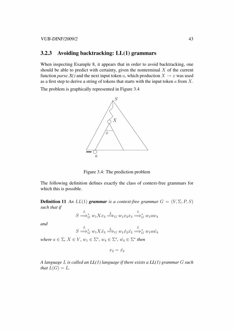
When inspecting Example 8, it appears that in order to avoid backtracking, oneshould be able to predict with certainty, given the nonterminal X of the currentfunction parse X() and the next input token a, which production X → x was usedas a first step to derive a string of tokens that starts with the input token a from X .
The problem is graphically represented in Figure 3.4
a
S
X
x
Figure 3.4: The prediction problem
The following definition defines exactly the class of context-free grammars forwhich this is possible.
Definition 11 An LL(1) grammar is a context-free grammar G = (V,Σ, P, S)such that if
SL
=⇒∗G w1Xx3L
=⇒G w1x2x3
L
=⇒∗G w1aw4
and
SL
=⇒∗G w1Xx3L
=⇒G w1x2x3
L
=⇒∗G w1aw4
where a ∈ Σ, X ∈ V , w1 ∈ Σ∗, w4 ∈ Σ∗, w4 ∈ Σ∗ then
x2 = x2
A language L is called an LL(1) language if there exists a LL(1) grammar G suchthat L(G) = L.

VUB-DINF/2009/2 44
Intuitively, Definition 11 just says that if there are two possible choices for a pro-duction, these choices are identical.
Thus for LL(1) grammars1, we know for sure that we can write functions as wedid in Example 8, without having to backtrack. In the next section, we will seehow to automatically generate parsers based on the same principle but without theoverhead of (possibly recursive) function calls.
3.2.4 Predictive parsers
Predictive parsers use a stack (representing strings in (V ∪ Σ)∗) and a parse tableas shown in Figure 3.5.
w a
input+ b $
Z
X
Y
stack
PREDICTIVEPARSER
parse table$
V × Σ→ P ∪ {error}
Figure 3.5: A predictive parser
The figure shows the parser simulating a leftmost derivation
SL
=⇒G . . .L
=⇒G wZY X︸ ︷︷ ︸depicted position of parser
L=⇒G . . .
L=⇒G wa+ b
Note that the string consisting of the input read so far, followed by the contentsof the stack (from the top down) constitutes a left sentential form. End markers(depicted as $ symbols) are used to mark both the bottom of the stack and the endof the input.
1It is possible to define LL(k) grammars and languages by replacing a in Definition 11 by aterminal string of (up to) k symbols.

VUB-DINF/2009/2 45
The parse table M represents the production to be chosen: when the parser has Xon the top of the stack and a as the next input symbol, M [X, a] determines whichproduction was used as a first step to derive a string starting with a from X .
Algorithm 2 [Operation of an LL(1) parser]The operation of the parser is shown in Figure 3.6. 2
Intuitively, a predictive parser simulates a leftmost derivation of its input, usingthe stack to store the part of the left sentential form that has not yet been processed(this part includes all nonterminals of the left sentential form). It is not difficultto see that if a predictive parser successfully processes an input string, then thisstring is indeed in the language generated by the grammar consisting of all therules in the parse table.
To see the reverse, we need to know just how the parse table is constructed.
First we need some auxiliary concepts:
Definition 12 Let G = (V,Σ, P, S) be a context-free grammar.
• The function first : (V ∪ Σ)∗ → 2(Σ∪{ε}) is defined by
first(α) = {a | α =⇒∗G aw ∈ Σ∗} ∪Xα
where
Xα =
{{ε} if α =⇒∗G ε∅ otherwise
• The function follow : V → 2(Σ∪{$}) is defined by
follow(A) = {a ∈ Σ | S =⇒∗G αAaβ} ∪ Yα
where
Yα =
{{$} if S =⇒∗G αA∅ otherwise
Intuitively, first(α) contains the set of terminal symbols that can appear at thestart of a (terminal) string derived from α, including ε if α can derive the emptystring.
On the other hand, follow(A) consists of those terminal symbols that may followa string derived from A in a terminal string from L(G).
The construction of the LL(1) parse table can then be done using the followingalgorithm.

VUB-DINF/2009/2 46
1 PRODUCTION* parse_table[NONTERMINAL,TOKEN];2 SYMBOL End, S; /* marker and start symbol */3 SYMBOL* stack;4 SYMBOL* top_of_stack;56 TOKEN *input;78 BOOL9 parse() { /* LL(1) predictive parser */
10 SYMBOL X;11 push(End); push(S);1213 while (*top_of_stack!=End) {14 X = *top_of_stack;15 if (is_terminal(X)) {16 if (X==*input) { /* predicted outcome */17 ++input; /* advance input */18 pop(); /* pop X from stack */19 }20 else21 error("Expected %s, got %s", X, *input);22 }23 else { /* X is nonterminal */24 PRODUCTION* p = parse_table[X,*input];25 if (p) {26 pop(); /* pop X from stack */27 for (i=length_rhs(p)-1;(i>=0);--i)28 push(p->rhs[i]); /* push symbols of rhs, last first */29 }30 else31 error("Unexpected %s", *input);32 }33 }34 if (*input==End)35 return true;36 else37 error("Redundant input: %s", *input);38 }
Figure 3.6: Predictive parser operation
Algorithm 3 [Construction of LL(1) parse table]Let G = (V,Σ, P, S) be a context-free grammar.
1. Initialize the table: ∀A ∈ V, b ∈ Σ ·M [A, b] = ∅
2. For each production A→ α from P

VUB-DINF/2009/2 47
(a) For each b ∈ first(α) ∩ Σ, add A→ α to M [A, b].
(b) If ε ∈ first(α) then
i. For each c ∈ follow(A) ∩ Σ, add A→ α to M [A, c].ii. If $ ∈ follow(A) then add A→ α to M [A, $].
3. If each entry in M contains at most a single production then return success,else return failure.
2
It can be shown that, if the parse table for a grammar G was successfully con-structed using Algorithm 3, then the parser of Algorithm 2 accepts exactly thestrings of L(G). Also, if Algorithm 3 fails, then G is not an LL(1) grammar.
Example 10 Consider grammar G2 from Example 9. The first and follow func-tions are computed in Examples 11 and 12. The results are summarized below.
E E ′ T T ′ Ffirst (, id +, ε (, id ×, ε (, idfollow $, ) $, ) +, $, ) $, ),+ ×, $, ),+
Applying Algorithm 3 yields the following LL(1) parse table.
E E ′ T T ′ F
id E → TE ′ T → FT ′ F → id+ E ′ → +TE ′ T ′ → ε× T ′ → ×FT ′( E → TE ′ T → FT ′ F → (E)) E ′ → ε T ′ → ε$ E ′ → ε T ′ → ε
The operation of a predictive parser using the above table is illustrated below for

VUB-DINF/2009/2 48
the input string id + id× id.
stack input rule$E id + id× id$$E ′T id + id× id$ E → TE ′
$E ′T ′F id + id× id$ T → FT ′
$E ′T ′id id + id× id$ F → id$E ′T ′ +id× id$$E ′ +id× id$ T ′ → ε$E ′T+ +id× id$ E ′ → +TE ′
$E ′T id× id$$E ′T ′F id× id$ T → FT ′
$E ′T ′id id× id$ F → id$E ′T ′ ×id$$E ′T ′F× ×id$ T ′ → ×FT ′$E ′T ′F id$$E ′T ′id id$ F → id$E ′T ′ $$E ′ $ T ′ → ε$ $ E ′ → ε
3.2.5 Construction of first and follow
Algorithm 4 [Construction of first]LetG = (V,Σ, P, S) be a context-free grammar. We construct an arrayF : V ∪ Σ→ 2(Σ∪{ε})
and then show a function to compute first(α) for arbitrary α ∈ (V ∪ Σ)∗.
1. F is constructed via a fixpoint computation:
(a) for each X ∈ V , initialize F [X]← {a | X → aα, a ∈ Σ}(b) for each a ∈ Σ, initialize F [a]← {a}
2. repeat the following steps
(a) F ′ ← F
(b) for each rule X → ε, add ε to F [X].
(c) for each rule X → Y1 . . . Yk (k > 0) do
i. for each 1 ≤ i ≤ k such that Y1 . . . Yi−1 ∈ V ∗ and ∀1 ≤ j < i · ε ∈ F [Yj]do F [X]← F [X] ∪ (F [Yi] \ {ε})
ii. if ∀1 ≤ j ≤ k · ε ∈ F [Yi] then F [X]← F [X] ∪ {ε}

VUB-DINF/2009/2 49
until F ′ = F
Define
first(X1 . . . Xn) =
{ ⋃1≤j≤(k+1)(F [Xj] \ {ε}) if k(X1 . . . Xn) < n⋃1≤j≤n F [Xj] ∪ {ε}) if k(X1 . . . Xn) = n
where k(X1 . . . Xn) is the largest index k such that X1 . . . Xk =⇒∗G ε, i.e.
k(X1 . . . Xn) = max{1 ≤ i ≤ n | ∀1 ≤ j ≤ i · ε ∈ F [Xj}
2
Example 11 Consider grammar G2 from Example 9.
The construction of F is illustrated in the following table.
E E ′ T T ′ F+ × (, id initializationε rule E ′ → ε
(, id rule T → FT ′
ε rule T ′ → ε(, id rule E → TE ′
(, id +, ε (, id ×, ε (, id
Algorithm 5 [Construction of follow]Let G = (V,Σ, P, S) be a context-free grammar. The follow set of all symbols inV can be computed as follows:
1. follow(S)← $
2. Apply the following rules until nothing can be added to follow(A) for anyA ∈ V .
(a) If there is a production A→ αBβ in P then
follow(B)← follow(B) ∪ (first(β) \ {ε})
(b) If there is a production A → αB or a production A → αBβ whereε ∈ first(β) then follow(B)← follow(B) ∪ follow(A).
2

VUB-DINF/2009/2 50
Example 12 Consider again grammar G2 from Example 9.
The construction of follow is illustrated in the following table.
E E ′ T T ′ F$ initialization
+ rule E → TE ′
) rule F → (E)× rule T → FT ′
$, ) rule E → TE ′
$, ) rule E → TE ′
$, ),+ rule T → FT ′
$, ),+ rule T → FT ′
$, ) $, ) +, $, ) $, ),+ ×, $, ),+
3.3 Bottom-up parsing
3.3.1 Shift-reduce parsers
As described in Section 3.2, a top-down parser simulates a leftmost derivation in atop-down fashion. This simulation predicts the next production to be used, basedon the nonterminal to be rewritten and the next input symbol.
A bottom-up parser simulates a rightmost derivation in a bottom-up fashion, wherea rightmost derivation is defined as follows.
Definition 13 LetG = (V,Σ, P, S) be a context-free grammar. For strings x, y ∈ (V ∪ Σ)∗,we say that x derives y in a rightmost fashion and in one step, denoted
xR
=⇒G y
iff x = x1Ax2, y = x1αx2, A → α is a rule in P and x2 ∈ Σ∗ (i.e. the rightmostoccurrence of a nonterminal symbol is rewritten).
The relationR
=⇒∗G is the reflexive and transitive closure of R=⇒G. A derivation
x0R
=⇒G x1R
=⇒G . . .R
=⇒G xn
is called a rightmost derivation. If x0 = S (the start symbol) then we call each xiin such a derivation a right sentential form.

VUB-DINF/2009/2 51
A phrase of a right sentential form is a sequence of symbols that have been de-rived from a single nonterminal symbol occurrence (in an earlier right sententialform of the derivation). A simple phrase is a phrase that contains no smallerphrase. The handle of a right sentential form is its leftmost simple phrase (whichis unique). A prefix of a right sentential form that does not extend past its handleis called a viable prefix of G.
Example 13 Consider the grammar
G3 = ({S,E, T, F}, {+,×, (, ), id}, PG3 , S)
where PG3 consists of
S → E
E → E + T | TT → T × F | FF → (E) | id
G3 is simply G1 from Example 7, augmented by a new start symbol whose onlyuse is at the left hand side of a single production that has the old start symbol asits right hand side.
The following table shows a rightmost derivation of id+id×id; where the handlein each right sentential form is underlined.
SEE + TE + T × FE + T × idE + F × idE + id× idT + id× idF + id× idid + id× id
When doing a bottom-up parse, the parser will use a stack to store the right senten-tial form up to the handle, using shift operations to push symbols from the inputonto the stack. When the handle is completely on the stack, it will be popped andreplaced by the left hand side of the production, using a reduce operation.

VUB-DINF/2009/2 52
Example 14 The table below illustrates the operation of a shift-reduce parser tosimulate the rightmost derivation from Example 13. Note that the parsing has tobe read from the bottom to the top of the figure and that both the stack and theinput contain the end marker “$”.
derivation stack input operationS $S $ acceptE $E $ reduce S → EE + T $E + T $ reduce E → E + TE + T × F $E + T × F $ reduce T → T × F
$E + T × id $ reduce F → id$E + T× id$ shift
E + T × id $E + T ×id$ shiftE + F × id $E + F ×id$ reduce T → F
$E + id ×id$ reduce F → id$E+ id× id$ shift
E + id× id $E +id× id$ shiftT + id× id $T +id× id$ reduce E → TF + id× id $F +id× id$ reduce T → F
$id +id× id$ reduce F → idid + id× id $ id + id× id$ shift
Clearly, the main problem when designing a shift-reduce parser is to decide whento shift and when to reduce. Specifically, the parser should reduce only when thehandle is on the top of the stack. Put in another way, the stack should alwayscontain a viable prefix.
We will see in Section 3.3.2 that the language of all viable prefixes of a context-free grammarG is regular, and thus there exists a DFAMG = (Q, V ∪ Σ, δ, q0, F )accepting exactly the viable prefixes of G. The operation of a shift-reduce parseris outlined in Figure 3.72.
However, rather than checking each time the contents of the stack (and the nextinput symbol) vs. the DFAMG, it is more efficient to store the states together withthe symbols on the stack in such a way that for each prefix xX of (the contentsof) the stack, we store the state δ∗(q0, xX) together with X on the stack.
In this way, we can simply check δMG(q, a) where q ∈ Q is the state on the top of
the stack and a is the current input symbol, to find out whether shifting the inputwould still yield a viable prefix on the stack. Similarly, upon a reduce(A → α)
2We assume, without losing generality, that the start symbol of G does not occur on the righthand side of any production

VUB-DINF/2009/2 53
1 while (true) {2 if ((the top of the stack contains the start symbol) &&3 (the current input symbol is the endmarker ’$’))4 accept;5 else if (the contents of the stack concatenated with the next6 input symbol is a viable prefix)7 shift the input onto the top of the stack;8 else9 if (there is an appropriate producion)
10 reduce by this production;11 else12 error;13 }
Figure 3.7: Naive shift-reduce parsing procedure
operation, both A and δ(q, A) are pushed where q is the state on the top of thestack after popping α.
In practice, a shift-reduce parser is driven by two tables:
• An action table that associates a pair consisting of a state q ∈ Q and asymbol a ∈ Σ (the input symbol) with an action of one of the followingtypes:
– accept , indicating that the parse finished successfully
– shift(q′), where q ∈ Q is a final state of MG. This action tells theparser to push both the input symbol and q on top of the stack. In thiscase δMG
(q, a) = q′.
– reduce(A → α) where A → α is a production from G. This in-structs the parser to pop α (and associated states) from the top ofthe stack, then pushing A and the state q′ given by q′ = goto(q′′, A)where q′′ is the state left on the top of the stack after popping α. Heregoto(q′′, A) = δMG
(q′′, A).
– error, indicating that δMG(q, a) yields a dead state.
• A goto table:goto : Q× V → Q
which is used during a reduce operation.
The architecture of a shift-reduce parser is shown in Figure 3.8.
Using the action and goto tables, we can refine the shift-reduce parsing algorithmas follows.

VUB-DINF/2009/2 54
input$
$
E
+
T
×
+ idid
q0
q1
q2
q3
q4 goto: V ×Q→ Q
stack
SHIFT-REDUCEPARSER
id×
action : Q× Σ→ ACTION
Figure 3.8: A shift-reduce parser
Algorithm 6 [Shift-reduce parsing]See Figure 3.9 on page 55. 2
3.3.2 LR(1) parsing
Definition 14 Let G = (V,Σ, P, S ′) be a context-free grammar such that S ′ → Sis the only production for S ′ and S ′ does not appear on the right hand side of anyproduction.
• An LR(1) item is a pair [A→ α •β, a] where A→ αβ is a production fromP , • is a new symbol and a ∈ Σ ∪ {$} is a terminal or end marker symbol.We use itemsG to denote the set of all items of G.
• The LR(1) viable prefix NFA of G is
NG = (itemsG, V ∪ Σ, δ, [S ′ → •S], itemsG)
where δ is defined by
[A→ αX • β, a] ∈ δ([A→ α •Xβ, a], X) for all X ∈ V ∪ Σ[X → •γ, b] ∈ δ([A→ α •Xβ, a], ε) if X → γ is in P and b ∈ first(βa)

VUB-DINF/2009/2 55
1 TOKEN* input; /* array of input tokens */2 STATE* states; /* (top of) stack of states */3 SYMBOL* symbols; /* (top of) stack of symbols */45 BOOL6 parse() {7 while (true)8 switch (action[*states,*input]) {9 case shift(s):
10 *++symbols = *input++; /* push symbol */11 *++states = s; /* push state */12 break;13 case reduce(X->x):14 symbols -= length(x); /* pop rsh */15 states -= length(x); /* also for states */16 STATE s = goto[*states,X];17 *++states = s; *++symbols = X;18 break;19 case accept:20 return true;21 case error:22 return false;23 }24 }
Figure 3.9: Shift-reduce parser algorithm
Note that all states in NG are final. This does not mean that NG accepts any stringsince there may be no transitions possible on certain inputs from certain states.
Intuitively, an item [A → α • β, a] can be regarded as describing the state wherethe parser has α on the top of the stack and next expects to process the result of aderivation from β, followed by an input symbol a.
To see that L(NG) accepts all viable prefixes. Consider a (partial)3 rightmostderivation
S = X0R
=⇒G x0X1y0
R
=⇒∗G x0x1X2y1
R
=⇒∗G x0 . . . xn−1XnynR
=⇒G x0 . . . xn−1xnyn
where yi ∈ Σ∗ for all 0 ≤ i ≤ n, as depicted in Figure 3.10 where we show onlythe steps involving the ancestors of the left hand side (Xn) of the last step (notethat none of the xi changes after being produced because we consider a rightmostderivation).
3By a partial rightmost derivation we mean a rightmost derivation that can be extended to asuccessful full rightmost derivation.

VUB-DINF/2009/2 56
X0
x0
x1
Xn
xn−1
xn
Xn−1
X2
X1b0 = $
b1
bn−2
bn−1
bn
Figure 3.10: A (partial) rightmost derivation
NG can accept any viable prefix of the right sentential form x0 . . . xn−1xnyn, i.e.any prefix of x0 . . . xn−1xn as follows:
[S ′ → •X0, $] the initial state[X0 → •x0X1z0, b0] using an ε-move, b0 ∈ first(ε$) = {$}[X0 → x0 •X1z0, b0] reading x0
[X1 → •x1X2z1, b1] using an ε-move, b1 ∈ first(z0b0)[X1 → x1 •X2z1, b1] reading x1
. . .[Xn−1 → •xn−1Xnzn−1, bn−1][Xn−1 → xn−1 •Xnzn−1, bn−1] reading xn−1
[Xn → •xn, bn] using an ε-move, bn ∈ first(zn−1bn−1). . . any prefix of xn can be read
Note that all bi exist since each zi derives a terminal string.
To see the reverse, it suffices to note that each accepting sequence in MG is ofthe form sketched above and thus, a partial rightmost derivation like the one inFigure 3.10 can be inferred from it.

VUB-DINF/2009/2 57
Theorem 4 Let G = (V,Σ, P, S ′) be a context-free grammar and let NG be itsviable prefix NFA. Then L(NG) contains exactly the viable prefixes of G.
Because of Theorem 1, we can convert NG to an equivalent DFA MG that can beused to build the action and goto tables of a shift-reduce parser as follows.
Algorithm 7 [Construction of LR(1) tables]Let
MG = (2itemsG , V ∪ Σ, δ, Cε([S ′ → •S, $]), 2itemsG \ {∅})
be the DFA corresponding to the viable prefix automaton NG of G.
• Add an action accept to action[s, $] whenever [S ′ → S•, $] ∈ s.
• Add an action shift(s′) to action[s, a] whenever δ(s, a) = s′.
• Add an action reduce(A → α) to action[s, a] whenever s contains an item[A→ α•, a] where A 6= S ′.
• For any X ∈ V , s a state of MG, define goto(s,X) = δ(s,X).
After the above rules have been exhaustively applied, add error to all entries inaction that remain empty.
The algorithm succeeds if action[s, a] contains exactly one action for each reach-able s ∈ 2itemsG , a ∈ Σ. 2
Note that it follows from Theorem 4 and Algorithm 7 that the resulting parser willannounce an error at the latest possible moment, that is only when shifting wouldresult in a stack that does not represent a viable prefix.
If Algorithm 7 does not succeed, there exists either a shift-reduce conflict,when an entry in the action table contains both a shift and a reduce operation, ora reduce-reduce conflict, when an entry in the action table contains two or morereduce actions.
Example 15 Consider G3 from Example 13. The DFA accepting the viable pre-fixes of G is shown in Figures 3.11 and 3.12 Note that [A→ α, abc] is used asshorthand for {[A→ α, a], [A→ α, b], [A→ α, c]
Theorem 5 Let G = (V,Σ, P, S ′) be a context-free grammar such that Algo-rithm 7 succeeds. Then Algorithm 6 accepts exactly L(G).

VUB-DINF/2009/2 58
State Items State Items0 S′ → •S $ 11 E → E + T• +$
S → •E $ T → T • ×F ×+ $E → •E + T +$ 12 F → (E•) ×+ $E → •T +$ E → E •+T )+T → •T × F ×+ $ 13 F → (E)• ×+ $T → •F ×+ $ 14 T → F• )×+F → •id ×+ $ 15 F → (E)• ) +×F → •(E) ×+ $ 16 F → (E•) ) +×
1 S → E• $ E → E •+T )+E → E •+T +$ 17 E → E + •T )+
2 S′ → S• $ T → •T × F ) +×3 E → E + •T +$ T → •F ) +×
T → •T × F ×+ $ F → •id ) +×T → •F ×+ $ F → •(E) ) +×F → •id ×+ $ 18 F → (•E) ) +×F → •(E) ×+ $ E → •E + T )+
4 T → F• ×+ $ E → •T )+5 F → id• ×+ $ T → •T × F ) +×6 F → (•E) ×+ $ T → •F ) +×
E → •E + T )+ F → •id ) +×E → •T )+ F → •(E) ) +×T → •T × F )×+ 19 E → T• )+T → •F )×+ T → T • ×F ) +×F → •id )×+ 20 E → E + T• )+F → •(E) )×+ T → T • ×F ) +×
7 E → T• +$ 21 T → T × •F ) +×T → T • ×F ×+ $ F → •id ) +×
8 T → T × •F ×+ $ F → •(E) ) +×F → •id ×+ $ 22 T → T × F• ) +×F → •(E) ×+ $
9 T → T × F• ×+ $10 F → id• )×+
Figure 3.11: States of the viable prefix DFA of G3
Example 16 The action and goto tables of the LR(1) parser for G3 are shown inFigure 3.13. The rules of G3 have been numbered as follows:
1 S → E 5 T → F2 E → E + T 6 F → id3 E → T 7 F → (E)4 T → T × F
A parse ofid + id× id

VUB-DINF/2009/2 59
δMG3S E T F id ( ) + ×
0 2 1 7 4 5 61 323 11 4 5 6456 19 14 10 187 88 9 5 69
1011 812 13 1713141516 1717 20 14 10 1818 19 14 10 1819 2120 2121 22 1022
Figure 3.12: Transition function of the viable prefix DFA of G3
is shown below (states on the stack are between “[]”).
stack input operation$[0] id + id× id$ shift$[0]id[5] +id× id$ reduce F → id$[0]F [4] +id× id$ reduce T → F$[0]T [7] +id× id$ reduce E → T$[0]E[1] +id× id$ shift$[0]E[1] + [3] id× id$ shift$[0]E[1] + [3]id[5] ×id$ reduce F → id$[0]E[1] + [3]F [4] ×id$ reduce T → F$[0]E[1] + [3]T [11] ×id$ shift$[0]E[1] + [3]T [11]× [8] id$ shift$[0]E[1] + [3]T [11]× [8]id[5] $ reduce F → id$[0]E[1] + [3]T [11]× [8]F [9] $ reduce T → T × F$[0]E[1] + [3]T [11] $ reduce E → E + T$[0]E[1] $ reduce S → E$[0]S[2] $ accept
It will turn out that Algorithm 7 succeeds exactly for so-called LR(1) grammars.

VUB-DINF/2009/2 60
goto actionstate S E T F id ( ) + × $
0 2 1 7 4 s5 s61 s3 r12 a3 11 4 s5 s64 r5 r5 r55 r6 r6 r66 19 14 s10 s187 r3 s8 r38 9 s5 s69 r4 r4 r4
10 r6 r6 r611 r2 s8 r212 s13 s1713 r7 r7 r714 r5 r5 r515 r7 r7 r716 s1717 20 14 s10 s1818 19 14 s10 s1819 r3 r3 s2120 r2 r2 s2121 22 s1022 r4 r4 r4
Figure 3.13: LR(1) tables for G3

VUB-DINF/2009/2 61
Definition 15 An LR(1) grammar is a context-free grammar G = (V,Σ, δ, P, S)such that S does not appear at the right hand side of any production. Moreover, if
SR
=⇒∗G x1Xw3R
=⇒G x1x2w3
and
SR
=⇒∗G x1Xw3R
=⇒G x1x2w3
andpref l+1(x1x2w3) = pref l+1(x1x2w3)
where X ∈ V , w3w3 ∈ Σ∗, l = |x1x2|, then
x1 = x1 ∧ X = X
A language L is called LR(1) if there exists an LR(1) context-free grammarG suchthat L(G) = L.
Intuitively, in the above definition, x1x2 represents the stack just before a reduceoperation in a shift-reduce parser. The definition then says that there is only asingle choice for when to reduce, based only on the next input symbol4.
Theorem 6 A context-free grammar G = (V,Σ, δ, P, S), where S does not ap-pear on the right hand side of any production, is LR(1) iff Algorithm 7 succeeds.
One may wonder about the relationship between LL(k) and LR(k) grammars andlanguages. It turns out (see e.g. [Sal73]) that every LR(k) (k ≥ 0) languagecan be generated by an LR(1) grammar. On the other hand, there are contextfree languages, e.g. the inherently ambiguous language of Section 3.1, page 38,that are not LR(1). In fact, it can be shown that all deterministic context-freelanguages5 are LR(1) (and, obviously, also the reverse). As for LL(k) languages,they form a proper hierarchy in that for every k > 1 there is an LL(k) languageLk for which no LL(k − 1) grammar exists. Still, every LL(k) language is LR(1).
Summarizing, as far as parsing power is concerned, bottom-up (LR(1)) parsersare provably superior to top-down (LL(1)) parsers.
4One can also define LR(k) grammars and languages for any k ≥ 0. It suffices to replace l+ 1by l + k in Definition 15
5A context-free language is deterministic if it can be accepted by a deterministic pushdownautomaton.

VUB-DINF/2009/2 62
3.3.3 LALR parsers and yacc/bison
LR(1) parsing tables can become quite large due to the large number of states inthe viable prefix DFA. A DFA for a language like Pascal may have thousands ofstates.
In an LALR parser, one tries to reduce the number of states by merging statesthat have the same (extended) productions in their items. E.g. in the DFA ofExample 15, one may merge, among others, state 3 and state 17.
It is then not hard to see that, due to the way states are constructed using ε-closures, if s1 and s2 can be merged, then so can δ(s1, X) and δ(s2, X). Thisyields a more compact DFA which is “almost” equivalent to the original one in thesense that compaction cannot produce shift-reduce conflicts although new reduce-reduce conflicts are possible.
It can be shown that if the LALR compaction succeeds (i.e. does not lead to newreduce-reduce conflicts), the resulting parser accepts the same language as theoriginal LR(1) parser.
The parser-generator yacc (and bison) generates an LALR parser based on aninput grammar. In addition, yacc (and bison) provide facilities for resolving shift-reduce conflicts based on the declared precedence of operators.
Bison will resolve a shift reduce conflict on a state like
E → Eo1E• , o2
E → E • o2E
by comparing the declared precedences of o1 and o2: if o1 has the higher prece-dence, then reduce will be selected. If o2 has a higher precedence than o1 then shiftwill be selected. If o1 and o2 have the same precedence, associativity informationon o1 and o2 will be used: if both symbols (operators) are left-associative, reducewill be selected; if both symbols are right-associative, shift will be selected; ifboth symbols are non-associative an error will be reported6. If a symbol (such asMINUS in Example 17 below) is used with two precedences, bison allows you todefine the precedence of the rule using a %prec directive7
The default conflict resolution strategy of bison (and yacc) is as follows:6Note that operators with the same precedence must have the same associativity.7The above description is made more concrete in the bison manual:
The first effect of the precedence declarations is to assign precedence levels to the terminalsymbols declared. The second effect is to assign precedence levels to certain rules: each rule getsits precedence from the last terminal symbol mentioned in the components (o1 in the example).(You can also specify explicitly the precedence of a rule.)

VUB-DINF/2009/2 63
• Choose shift when resolving a shift-reduce conflict.
• Choose reduce by the first production (in the order of declaration) whenresolving a reduce-reduce conflict.
Example 17 The following is the bison input file for a highly ambiguous gram-mar, where ambiguities are resolved using the precedence/associativity definingfacilities of bison/yacc.
12 %token NAME NUMBER LPAREN RPAREN EQUAL PLUS MINUS3 %token TIMES DIVIDE IF THEN ELSE45 /* associativity and precedence: in order of increasing precedence */67 %nonassoc LOW /* dummy token to suggest shift on ELSE */8 %nonassoc ELSE /* higher than LOW */9
10 %nonassoc EQUAL11 %left PLUS MINUS12 %left TIMES DIVIDE13 %left UMINUS /* dummy token to use as precedence marker */1415 %%1617 stmt : IF exp THEN stmt %prec LOW18 | IF exp THEN stmt ELSE stmt /* shift will be selected */19 | /* other types of statements would come here */20 ;2122 exp : exp PLUS exp23 | exp MINUS exp24 | exp TIMES exp25 | exp DIVIDE exp26 | exp EQUAL exp27 | LPAREN exp RPAREN28 | MINUS exp %prec UMINUS /* this will force a reduce */29 | NAME30 | NUMBER
Finally, the resolution of conflicts works by comparing the precedence of the rule (of o1 in theexample, unless that rule’s precedence has been explicitly defined) being considered (for reduce)with that of the look-ahead token (o2 in the example). If the token’s precedence is higher, thechoice is to shift. If the rules precedence is higher, the choice is to reduce. If they have equalprecedence, the choice is made based on the associativity of that precedence level. The verboseoutput file made by ‘-v’ (see section Invoking Bison) says how each conflict was resolved.
Not all rules and not all tokens have precedence. If either the rule or the look-ahead token hasno precedence, then the default is to shift.

VUB-DINF/2009/2 64
31 ;32 %%

Chapter 4
Checking static semantics
4.1 Attribute grammars and syntax-directed trans-lation
Attribute grammars extend context-free grammars by associating a set of attributeswith each grammar symbol. Such attributes can be used to present informationthat cannot easily (if at all) be expressed using only syntactical constructs (e.g.productions). Thus each node in a parse tree has values for each of the attributesassociated with the corresponding symbol.
For example, we could associate an attribute type with the nonterminal expressionto represent the type of the expression.
Attributes for nodes are computed using functions that take attribute values ofother nodes as input. The computation is specified by semantic actions whichare associated with each production. Since such actions can only reference thesymbols in the production, the value of an attribute of a node depends only on theattribute values of its parent, children and siblings.
Example 18 Consider the grammar
G4 = ({E}, {+,×,−, /, (, ),number}, P, E)
where P consists of
E → number | (E) | E + E | E × E | E/E | E − E | −E
We define an attribute value for E and number. The semantic actions are asfollow:
65

VUB-DINF/2009/2 66
E.value = 12
E.value = 24
+
E.value = 4
number.value = 4
number.value = 3
×
number.value = 12
E.value = 12
E.value = 3
Figure 4.1: Computing synthesized attribute values
E → number E0.value = number1.valueE → (E) E0.value = E1.valueE → E + E E0.value = E1.value + E3.valueE → E × E E0.value = E1.value × E3.valueE → E − E E0.value = E1.value − E3.valueE → E/E E0.value = E1.value/E3.valueE → −E E0.value = −E1.value
Note that we use subscripts to refer to a particular occurrence of a symbol in therule (subscript 0 is used for the left-hand side of the rule).
The attribute values for a parse tree of 12 + 3 ∗ 4 are shown in Figure 4.1. Notethat the number.value is supposed to have been provided by the lexical analyzer.
The actions in Example 18 all compute an attribute value for a node based on theattribute values of its children. Attributes that are always computed in this wayare called synthesized attributes. Attributes whose value depends on values of itsparent and/or siblings are called inherited attributes.
The following example shows a grammar with both synthesized and inheritedattributes.

VUB-DINF/2009/2 67
Example 19 Consider the grammar
G5 = ({D,T, L}, {′,′ , ; , id, int,double}, P,D)
HereD represents a C-style declaration consisting of a type followed by a comma-separated list of identifiers. The symbols T , L, and id have a type attribute whichis inherited for L and id.
The productions and actions of P are
D → TL; L2.type = T1.typeT → int T0.type = intT → double T0.type = doubleL → L, id L1.type = L0.type
id3.type = L0.typeL → id id1.type = L0.type
The attribute values for the parse tree of
int x,y,z;
are shown in Figure 4.2. The dependencies between values are shown by dashedarrows.
In general, one can define a dependency graph for a parse tree where the nodesare pairs (n, a) where n is a node in the parse tree and a is an attribute for (thesymbol of) n. There is an edge from (n1, a1) to (n2, a2) if the value of n2.a2
depends on the value of (n1, a1), i.e. an action computing n2.a2 uses (n1, a1).
Attribute values can then be computed in any order that corresponds to a topo-logical sort1 of the nodes of the dependency graph. Clearly, for this to work, thedependency graph may not contain a cycle.
Thus, the syntax-directed translation G(α) of an input string α using an attributegrammar G can be computed by executing the following steps:
1. Parse α, according to the context-free grammar underlying G, yielding aparse tree tα.
2. Construct the dependency graph gtα , and compute the attribute values of thenodes of tα as described above.
1A topological sort of a directed (acyclic) graph is any total orderingx1 < x2 < . . . < xn < . . . of the nodes of the graph that satisfies xi < xj whenever thereis an edge from xi to xj .

VUB-DINF/2009/2 68
x
,
L.type = inty
id.type = int
L.type = int
D
;
id.type = int
z,
L.type = int
id.type = int
T.type = int
Figure 4.2: Computing inherited attribute values
3. G(α) is the value corresponding to some selected attribute of the root of tα.
In practice, the full parse tree for an input program is often not explicitly con-structed. Rather, attributes are computed and stored on a stack that mirrors theparsing stack (just like the stack containing the states of the viable prefix DFA)and actions are performed upon a reduce operations. This allows computationof synthesized attributes but inherited attributes are not easily supported althoughin certain cases it is possible to also evaluate inherited attributes (see [ASU86],pages 310-311).
In yacc and bison, each symbol (nonterminal or token) can have only one at-tribute, not larger than a single word. The type of an attribute is fixed per symbolusing %type declarations, as can be seen in the example parser in Appendix C.6,page 175. The set of used types must also be declared in a %union declaration.The restriction to a single word is not limiting: usually the attribute is declared tobe a pointer to a structure.
4.2 Symbol tables
The restriction of shift-reduce parsers to use only synthesized attributes can beovercome by using a global symbol table to share information between various

VUB-DINF/2009/2 69
parts of the parse tree. In general, a symbol table maps names (of variables, func-tions, types, . . . ) to information on this name which has been accumulated by theparser and semantic actions.
We discuss two aspects of symbol tables:
• The management of names (the domain of the mapping).
• The organization of the symbol table to take into account the scope rules ofthe language.
4.2.1 String pool
Since a symbol table maps names to information, one could implement a symboltable entry as a structure where the first field is the name and the other fieldscontain the information associated with the name
1 struct symtab_entry {2 char name[MAX_NAME_LENGTH];3 INFO info;4 };
However, because modern programming languages do not impose a small limiton the length of a name, it is wasteful or impossible to keep this organization.Hence one typically stores names contiguously in a so-called “string pool” array,declaring a symbol table entry as follows:
1 struct symtab_entry {2 char* name; /* points into string pool */3 INFO info;4 };
For fast retrieval, entries may be organized into a hash table, as illustrated inFigure 4.3 where separate chaining is used to link entries that correspond to thesame hash value.
4.2.2 Symbol tables and scope rules
Many programming languages impose scope rules that determine which defini-tion of a name corresponds to a particular occurrence of that name in a programtext. E.g. in Pascal, and in C, scopes may be nested to an arbitrary depth, as isillustrated in the following fragment.

VUB-DINF/2009/2 70
a b c \0 a l o n g i s h n a m e \0 x y z u \0
symbol table entry
hash table
Figure 4.3: A simple symbol table using a string pool and hashing
1 float x; /* def 1 */23 int4 f(int a)5 {6 while (a>0) {7 double x = a*a,i; /* def 2 */89 for (i=0;(i<a);++i) {
10 int x = a+i,b; /* def 3 */11 b = x+2; /* refers to def 3 */12 }1314 }15 }
In the above examples, the symbol table will contain three entries (definitions) forx at the time the inner loop is processed. Which definition is meant is determinedusing the “most closely nested scope” rule.
In a compiler for a language with scope rules, when a semantic action wants toretrieve the information associated with a certain occurrence of a name, it has toknow which definition of the name corresponds to the given occurrence. If thelanguage allows only nested scopes for which the “most closely nested scope”rule holds, this can be solved by replacing the symbol table by a stack of simple

VUB-DINF/2009/2 71
scope
current scopestring pool
parent
Figure 4.4: A stacked symbol table
symbol tables, one for each scope. Moreover, each simple table refers to its parentin the stack which contains symbol definitions from the enclosing scope. Whenlooking up a name, it suffices to search the simple table at the top of the stack. Ifthe name is not found, the parent table (corresponding to the enclosing scope) issearched and so on.
When the parser finishes a scope it pops the current scope from the stack andcontinues with the parent scope as the current one. Of course, if the scope is stillneeded, as is the case e.g. in C++ with scopes that correspond to class declara-tions, the scope will not be thrown away but a reference to it will be kept, e.g. inthe symbol table entry corresponding to the class name.
This organization is depicted in Figure 4.4.
An simple implementation of this scheme, where hashing is replaced by linearsearch (first in the current scope, then in the parent scope), may be found in Ap-pendix C.3, page 163.
4.3 Type checking
Informally, the so-called static semantics of a programming language describesthe properties of a program that can be verified without actually executing it. Typ-ically, for statically-types languages, this consists of verifying the “well-typed”property where a program is well-typed if all its constructs (statements, expres-sions, . . . ) obey the type rules of the language.
The type system of a programming language consists of
• A definition of the set of all possible types.

VUB-DINF/2009/2 72
• Type rules that determine the type of a language construct.
The language from Appendix C, Minic, has two primitive types: integers andfloats and a few type constructors, as shown by the following domain2 definition3:
type :: int:: float:: array(type):: struct(tenv):: type∗ → type
tenv :: name → type
Note that the above definition is more general than is actually needed in Minic,which has no higher order functions. E.g. it is not possible to define a functionwith type
int→ (int→ int)
in Minic.
The type rules of Minic can be symbolically represented as follows (we use x : t todenote that x has type t). In the table below we use + to use any of the arithmeticoperators +,×, /,−.
t x; ⇒ x : t // declaration of xx : int ∧ y : int ⇒ (x+ y) : int
x : float ∧ y : float ⇒ (x+ y) : float
x : t ∧ y : t ⇒ (x == y) : int // support = test on any typex : array(t) ∧ i : int ⇒ x[i] : t
x : struct(s) ∧ n ∈ dom(s) ⇒ x.n : s(n)
x = e ∧ x : t ∧ e : t′ ∧ t 6= t′ ⇒ error
∀1 ≤ i ≤ n · xi : ti ∧ f : t1t2 . . . tn → t ⇒ f(x1, . . . , xn) : t
return x ∧ x : t′ ∧ f : t1t2 . . . tn → t ∧ t′ 6= t ⇒ error // within the body of f
Here error is used to indicate that a certain construct is not well-typed, i.e. notype can be assigned to it without violating the type rules.
2See e.g. the “Foundations of Computer Science II” course.3Note that there is no boolean type: like C, Minic uses integers instead of booleans.

VUB-DINF/2009/2 73
Type checking then consists of using the rules to assign a type to each expression,variable etc. If no type, or more than one type, can be assigned to a construct, orif the rules generate error, the program is not well-typed.
It should be obvious that with the help of attributes, semantic actions and a symboltable, such type checking is possible. An example of a type-checking parser forMinic can be found in Appendix C. In the example implementation, types arerepresented by structures where each structure contains a tag corresponding to thetype constructor. Furthermore, types are shared, which saves space and facilitateslater checking for equality (only pointers must be compared).
Note that there are statically typed languages (e.g. ML or Haskell) that do notrequire, as Minic does, that each variable is declared to have a specific type. In-stead, the type of a variable is inferred from its use. In addition, such languagesusually have a more sophisticated type system where types can have variables thatmay be instantiated. In this way, a language can allow for polymorphism where afunction has several (possibly an infinite number of) types.
A similar feature is supported by C++ through the template facility. E.g. a func-tion
1 template <class T>2 int length(list<T>) {3 // ...4 }
has a type list(α)→ int where α is a type variable. The compiler will instantiateα to int when processing the expression length(l) in
1 list<int> l;23 length(l);

Chapter 5
Intermediate code generation
While it is possible to construct a compiler that translates the source text directlyinto the target language, especially if sophisticated optimization is not required,there are important advantages of using an intermediate representation:
• It facilitates retargeting. A compiler employing an intermediate representa-tion can be viewed as consisting of a “front end” (everything up to interme-diate code generation1) and a “back end” (optimization, code generation).Note that all dependencies on the source language are located in the frontend while dependencies on the target language are confined to the back end.Thus, to retarget the compiler (i.e. to generate code for another processor),it suffices to adapt the back end only. Similarly, if the intermediate code issufficiently general, the back end could be reused in a compiler for anotherlanguage.
• Many machine-independent optimizations, especially those that require codemovement etc., can be done more easily on intermediate code.
Several forms of intermediate code have been proposed (and used):
• Postfix notation.
• Abstract syntax trees.
• Three-address code.1Any machine-independent optimization that can be performed on the intermediate code
should also be done in the front end.
74

VUB-DINF/2009/2 75
5.1 Postfix notation
Postfix notation, also called “postfix Polish” after the originator J. Lukasiewicz,represents expressions and flow of control statements in postfix form, which isfree of parentheses, as in the following example:
infix postfixa+ b ab+(a+ b)× (c− d) ab+ cd−×
In general, an expression consisting of a k-ary operator θ, applied on k (sub)expressionse1, . . . , ek is represented as
e′1e′2 . . . e
′kθ
where e′i, 1 ≤ i ≤ k, is the postfix form of ei.
Evaluation of postfix expressions is trivial, provided one uses an operand stack, asshown below.
1 operand2 eval_operator(OPERATOR o,item args[]);34 operand5 eval_postfix(item code[],int code_len)6 {7 operand stack[MAX_STACK];8 int tos = 0; // top of stack9
10 for (int i=0;(i<code_len);++i)11 if (is_operand(code[i]))12 stack[tos++] = code[i]; // push on stack13 else14 { // operator: pop args, eval, push result15 k = arity(code[i]);16 stack[tos-k] = eval_operator(code[i].oprtr, stack-k);17 tos -= (k-1);18 }19 return stack[0];20 }
By introducing labels which refer to a position in the postfix expression, arbitrarycontrol structures can be implemented using instructions like
label jump
e1e2 label jumplt

VUB-DINF/2009/2 76
In order to interpret labels and jump instructions, the above algorithm must ofcourse be extended to use a program counter (an index in the code array),
Postfix notation is attractive because it can be easily generated using syntax-directed translation. Below, we use an synthesized attribute code representingthe postfix notation of the corresponding symbol occurrence. The statementsassociated with a rule define the attribute of the left hand side of the rule (denoted$$), based on the attribute values of the symbols in its right hand side ($i refers tothe i’th symbol in the rules right hand side).
1 exp : exp binop exp {2 $$.code = concat($1.code, $3.code, operator($2));3 }4 exp : ( exp) {5 $$.code = $1.code;6 }7 exp : var { $$.code = $1; /* probably a symtab ref */ }
This scheme has the so-called simple postfix property which means that for a pro-duction
A→ A1A2 . . . An
the generated code is such that2
code(A) = code(A1) + . . .+ code(An) + tail
which implies that code can be emitted as soon as a reduction occurs.
Postfix code is often used for stack-oriented virtual machines without general pur-pose registers, such as the Java virtual machine (see e.g. the micro compiler inAppendix B. It is not particularly suitable for optimization (code movement ishard).
5.2 Abstract syntax trees
Abstract syntax trees are “pruned” parse trees where all nodes that contain re-dundant (e.g. with respect to the tree structure) information have been removed.Indeed, many nodes in the parse tree result from syntactic sugar in the grammarwhich is needed to ensure that the language can be efficiently parsed. Once wehave parsed the text, there is no need to keep these superfluous nodes3. E.g. theabstract syntax tree corresponding to the parse tree of Figure 1.6 on page 14 isshown in Figure 5.1.
2We use + to denote concatenation.3It should be noted that a formal definition of a language’s semantics is often based on a so-
called abstract syntax which only specifies the structure of the language’s constructs, rather than

VUB-DINF/2009/2 77
<program>
<statement> <statement_list>
<statement> <statement_list>
<assignment>
(xyz)
<NAME>
<statement>
<write_statement>(xyz)
<NAME>
<declaration>
<MINUS>
<PLUS>
<NUMBER>
(33)
<NUMBER>
(3)
<NUMBER>
(35)
<statement_list>
<>
<var>
<NAME>
(xyz)
Figure 5.1: Abstract syntax tree corresponding to the program in Figure 1.3
Abstract syntax trees (and directed acyclic graphs), particularly of expressions,are useful for certain optimizations such as common subexpression eliminationand optimal register allocation (for expression computation).
An abstract syntax tree can be generated using synthesized attributes.1 exp : exp binop exp {2 $$.tree = new_node_2($2,$1.tree,$3,tree);3 }4 %*5 exp : ( exp ) {6 $.tree = $2.tree;7 }8 %*9 exp : unop exp {
10 $$.tree = new_node_1($1,$2.tree);11 }12 %*13 exp : var {14 $$.tree = new_node_0($1);15 }
Abstract syntax trees can also be constructed for complete source texts. They then
the concrete syntax. E.g. in the abstract syntax specification, one would have a rule
assignment → var expression
rather thanassignment → var = expression
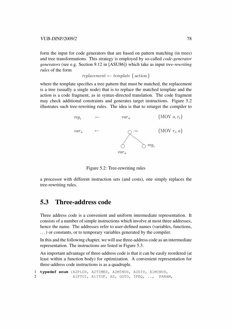
VUB-DINF/2009/2 78
form the input for code generators that are based on pattern matching (in trees)and tree transformations. This strategy is employed by so-called code-generatorgenerators (see e.g. Section 9.12 in [ASU86]) which take as input tree-rewritingrules of the form
replacement ← template { action }
where the template specifies a tree pattern that must be matched, the replacementis a tree (usually a single node) that is to replace the matched template and theaction is a code fragment, as in syntax-directed translation. The code fragmentmay check additional constraints and generates target instructions. Figure 5.2illustrates such tree-rewriting rules. The idea is that to retarget the compiler to
reg i
vara ←
← vara
:=
vara
reg i
{MOV ri, a}
{MOV a, ri}
Figure 5.2: Tree-rewriting rules
a processor with different instruction sets (and costs), one simply replaces thetree-rewriting rules.
5.3 Three-address code
Three address code is a convenient and uniform intermediate representation. Itconsists of a number of simple instructions which involve at most three addresses,hence the name. The addresses refer to user-defined names (variables, functions,. . . ) or constants, or to temporary variables generated by the compiler.
In this and the following chapter, we will use three-address code as an intermediaterepresentation. The instructions are listed in Figure 5.3.
An important advantage of three-address code is that it can be easily reordered (atleast within a function body) for optimization. A convenient representation forthree-address code instructions is as a quadruple.
1 typedef enum {A2PLUS, A2TIMES, A2MINUS, A2DIV, A1MINUS,2 A1FTOI, A1ITOF, A0, GOTO, IFEQ, .., PARAM,

VUB-DINF/2009/2 79
opcode instruction meaningA2(binop) A = B binop C assignment, binop can be +, ×, . . .A1(unop) A = unop B assignment, unop can be −, float2int, . . .A0 A = B simple assignmentGOTO goto labelIF(relop) if A relop B goto label relop can be <, >, ≤, ==, . . .PARAM param A push parameter before function callCALL call F, n function call, n is number of parametersAAC A = B[I] array access, B contains base address, I is offset in memory unitsAAS A[I] = B array modification, A contains base addressADDR A = address B take address of BDEREF A = * B as in CDEREFA *A = B as in CRETURN RETURN A as in C
Figure 5.3: Three-address code instructions
3 CALL, AAC, AAS, ADDR, DEREF, DEREFA } OPCODE;4 typedef struct {5 OPCODE op_code;6 SYM_INFO* args[2];7 SYM_INFO* result;8 } INSTRUCTION;
5.4 Translating assignment statements
The actions below use a simplified grammar for expressions. Also, we assumethat all expressions are of type integer.
We use two synthesized attributes:
• exp.place represents a reference to the location (variable, symbol table ref-erence) containing the value of the expression exp.
• exp.code represents the sequence of three-address statements computing thevalue of exp. Code concatenation is written as “+”.
1 extern INSTRUCTION /* create quadruple representing instruction */2 gen3ai(short op_code,SYM_INFO* arg1, SYM_INFO* arg2, SYM_INFO* result);34 assign : var = exp {5 $$.code = $3.code + gen3ai(A0,$3.place,0,$1.place);

VUB-DINF/2009/2 80
6 }7 exp : exp + exp {8 $$.place = newvar();9 $$.code = $1.code + $3.code
10 + gen3ai(A2PLUS,$1.place,$3.place,$$.place);11 }12 exp : - exp {13 $$.place = newvar();14 $$.code = $2.code15 + gen3ai(A1MINUS,$2.place,0,$$.place);16 }17 exp : ( exp ) {18 $$.place = $2.place;19 $$.code = $2.code;20 }21 exp : var {22 $$.place = $1.place;23 $$.code = 0;24 }
Note that the actions for the code attribute have the “simple postfix” property.Hence we can simplify the actions.
1 extern void2 emit(INSTRUCTION i);34 assign : var = exp {5 emit(gen3ai(A0,$3.place,0,$1.place));6 }7 exp : exp + exp {8 $$.place = newvar();9 emit(gen3ai(A2PLUS,$1.place,$3.place,$$.place));
10 }11 exp : - exp {12 $$.place = newvar();13 emit(gen3ai(A1MINUS,$2.place,0,$$.place));14 }15 exp : ( exp ) {16 $$.place = $2.place;17 }18 exp : var {19 $$.place = $1.place;20 }
As an example of the integration of static (notably type) checking with interme-diate code generation, we show below how appropriate conversions can be gen-erated for languages that support them. Note that we use an extra attribute typerepresenting the type of an expression, which can be either t int (integer) ort float (floating point). We also assume that there are two instructions for

VUB-DINF/2009/2 81
addition: A2PLUSI and A2PLUSF for integer and floating point addition, re-spectively.
1 exp : exp + exp {2 $$.place = newvar();3 if (($1.type==t_int)&&($3.type==t_int)) {4 $$.type = t_int; symtab_set_type($$.place,t_int);5 emit(gen3ai(A2PLUSI,$1.place,$3.place,$$.place));6 }7 else if (($1.type==t_float)&&($3.type==t_float)) {8 $$.type = t_float; symtab_set_type($$.place,t_float);9 emit(gen3ai(A2PLUSF,$1.place,$3.place,$$.place));
10 }11 else if (($1.type==t_int)&&($3.type==t_float)) {12 SYM_INFO* tmpf = newvar(t_float);13 emit(gen3ai(A1ITOF,$1.place,0,tmpf));14 $$.type = t_float; symtab_set_type($$.place,t_float);15 emit(gen3ai(A2PLUSF,$1.place,tmpf,$$.place));16 }17 else if (($1.type==t_float)&&($3.type==t_int)) {18 SYM_INFO* tmpf = newvar(t_float);19 emit(gen3ai(A1ITOF,$3.place,0,tmpf));20 $$.type = t_float; symtab_set_type($$.place,t_float);21 emit(gen3ai(A2PLUSF,tmpf,$3.place,$$.place));22 }23 }
5.5 Translating boolean expressions
First we consider the translation of boolean expressions (conditions). An obviouspossibility is to translate such expressions by value, i.e. by creating, if necessary,a temporary variable to hold its value. In this case, we agree to use 0 to represent“false” and 1 to represent “true”.
1 extern int2 next3ai(); /* returns number of next (free) location in code sequence */34 bexp : bexp OR bexp {5 $$.place = newvar(t_bool);6 emit(gen3ai(A2OR,$1.place,$3.place,$$.place));7 }89 bexp : bexp > bexp {
10 $$.place = newvar(t_bool);11 emit(gen3ai(IFGT,$1.place,$3.place,next3ai()+3));12 emit(gen3ai(A0C,0,0,$$.place));
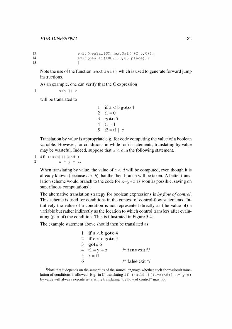
VUB-DINF/2009/2 82
13 emit(gen3ai(GO,next3ai()+2,0,0));14 emit(gen3ai(A0C,1,0,$$.place));15 }
Note the use of the function next3ai() which is used to generate forward jumpinstructions.
As an example, one can verify that the C expression1 a<b || c
will be translated to
1 if a < b goto 42 t1 = 03 goto 54 t1 = 15 t2 = t1 || c
Translation by value is appropriate e.g. for code computing the value of a booleanvariable. However, for conditions in while- or if-statements, translating by valuemay be wasteful. Indeed, suppose that a < b in the following statement.
1 if ((a<b)||(c<d))2 x = y + z;
When translating by value, the value of c < d will be computed, even though it isalready known (because a < b) that the then-branch will be taken. A better trans-lation scheme would branch to the code for x=y+z as soon as possible, saving onsuperfluous computations4.
The alternative translation strategy for boolean expressions is by flow of control.This scheme is used for conditions in the context of control-flow statements. In-tuitively the value of a condition is not represented directly as (the value of) avariable but rather indirectly as the location to which control transfers after evalu-ating (part of) the condition. This is illustrated in Figure 5.4.
The example statement above should then be translated as
1 if a < b goto 42 if c < d goto 43 goto 64 t1 = y + z /* true exit */5 x = t16 /* false exit */
4Note that it depends on the semantics of the source language whether such short-circuit trans-lation of conditions is allowed. E.g. in C, translating if ((a<b)||((u=z)<d)) x= y+z;by value will always execute u=z while translating “by flow of control” may not.

VUB-DINF/2009/2 83
C S goto
false
true S’ goto S”C
if C then S’ else S”
while C S
false
true
Figure 5.4: Conditional control flow statements
Thus a condition is associated with two locations in the code: a true and falseexit. The generated code is such that control will transfer to the true or false exitas soon as possible. However, as can be seen in Figure 5.4, the exits are usuallyunknown when the condition is parsed, since they refer to locations further in thecode array. The solution is to generate a dummy “goto ?” instruction wherever ajump to an exit should come. Here “?” is a placeholder for the, as yet unknown,location of the exit. The locations of the dummy jump instructions are kept in twosynthesized attributes associated with the condition:
• bexp.true contains the set of all “goto ?” instructions generated so far where“?” should eventually be replaced by the address of the true exit.
• bexp.false contains the set of all “goto ?” instructions generated so far where“?” should eventually be replaced by the address of the false exit.
When the exact location l of e.g. the true exit becomes known, one can backpatchthe instructions in bexp.true, replacing “?” by l in each of them.
The semantics of boolean operations such as disjunction, conjunction and nega-tion can easily be expressed by manipulation of the true and false sets, as illus-trated in Figure 5.5.
The actions are shown below.12 cond : cond AND marker cond {3 $$.true = $4.true;

VUB-DINF/2009/2 84
E1 E2
E1 ∧ E2
true truefalse
false
true
Figure 5.5: Exit sets after “and”
4 backpatch($1.true,$3.location);5 $$.false = locations_union($1.false,$4.false);6 }7 marker : /* empty right hand side */ {8 $$.location = next3ai();9 }
10 cond : NOT cond {11 $$.true = $2.false;12 $$.false = $2.true;13 }14 cond : var {15 $$.true = locations_add(locations_create_set(),next3ai());16 emit(gen3ai(IFNEQ,$1.place,0,0)); /* true, backpatch later */17 $$.false = locations_add(locations_create_set(),next3ai());18 emit(gen3ai(GOTO,0,0,0)); /* false,backpatch later */19 }20 cond : exp < exp {21 $$.true = locations_add(locations_create_set(),next3ai());22 emit(gen3ai(IFLT,$1.place,$3.place,0)); /* true, backpatch later */23 $$.false = locations_add(locations_create_set(),next3ai());24 emit(gen3ai(GOTO,0,0,0)); /* false,backpatch later */25 }
Note the dummy marker → ε production: since it is reduced just before code forthe second bexp will be generated, it can be used to store the location of the startof this code in an attribute marker.location.
The following example illustrates the translation of1 p<q || (r<s && t<u)
The generated intermediate code is shown below:

VUB-DINF/2009/2 85
100 if p < q goto ?t /* true exit */101 goto 102102 if r < s goto 104103 goto ?f /* false exit */104 if y < u goto ?t /* true exit */105 goto ?f /* false exit */
5.6 Translating control flow statements
We will use the following example grammar:
stmt → if cond stmt else stmt| while cond stmt| { slist }| assign
slist → slist ; stmt| stmt
Observe that the code corresponding to a stmt, e.g. a while statement, may con-tain forward references to a “next” location (meaning, after the code of the presentstatement) which is unknown at the time code is generated for the current state-ment. Therefore we use an attribute stmt.next which contains the locations con-taining instructions that need to be backpatched with the location of the first state-ment after the current one. We will also use dummy nonterminals to mark certainlocations in the code. The actions for the above grammar are shown below.
1 marker : /* empty */ {2 $$.location = next3ai();3 }45 goend : /* empty */ {6 $$.next = locations_add(locations_create_set(),next3ai());7 emit(gen3ai(GOTO,0,0,0)); /* goto end,backpatch later */8 }9
10 stmt : IF cond marker stmt goend ELSE marker stmt {11 backpatch($2.true,$3.location);12 backpatch($2.false,$7.location);13 $$.next = locations_union(14 locations_union($4.next,$5.next),15 $8.next);16 }17

VUB-DINF/2009/2 86
18 stmt : WHILE marker cond marker stmt {19 backpatch($3.true,$4.location);20 backpatch($5.next,$2.location);21 $$.next = $3.false;22 emit(gen3ai(GOTO,$2.location,0,0));23 }2425 stmt : assign {26 $$.next = locations_create_set();27 }2829 stmt : LBRACE slist RBRACE {30 $$.next = $2.next;31 }3233 slist : stmt {34 $$.next = $1.next;35 }3637 slist : slist SEMICOLON marker stmt {38 backpatch($1.next,$3.location);39 $$.next = $4.next;40 }
The following example illustrates the translation of1 while (a<b)2 if (c<d)3 x = y + z;
The generated intermediate code is shown below:
100 if a < b goto 102101 goto 107102 if c < d goto 104103 goto 100 /* false exit */104 t = y + z105 x = t106 goto 100
5.7 Translating procedure calls
We will use the following example grammar:

VUB-DINF/2009/2 87
stmt → id( arg list )arg list → arg list , exp
| exp
Note that, as in C, we assume that all parameters are passed “by value”. If, ase.g. in Pascal or C++, the source language also supports passing parameters “byaddress”, extra instructions that take the address of an operand, may need to beinserted before the PARAM instruction.
A statement such as1 f(e1,e2)
will be translated as
.. .. /* code for e1, place t1 */
.. .. /* code for e2, place t2 */102 param t1103 param t2104 call f
The actions are:1 typedef struct place_list {2 ...3 } PLACE_LIST;45 typedef struct {6 ..7 } PLACE_LIST_CURSOR;89 /*
10 * list of places, return new list after successful operation11 */12 PLACE_LIST* place_list_create();13 void place_list_destroy(PLACE_LIST*);14 PLACE_LIST* place_list_append(PLACE_LIST*,SYM_INFO*);1516 /*17 * cursor into list of places, return null pointer upon failure.18 */19 PLACE_LIST_CURSOR* place_list_first(PLACE_LIST*);20 void place_list_cursor_destroy(PLACE_LIST_CURSOR*);21 PLACE_LIST_CURSOR* place_list_next(PLACE_LIST_CURSOR*);22 SYM_INFO* place_list_current(PLACE_LIST_CURSOR*);2324 stmt : ID ( arg_list) {

VUB-DINF/2009/2 88
25 PLACE_LIST_CURSOR* c;26 int n = 0; /* number of arguments */2728 while (c = place_list.first($3.places)) {29 ++n;30 emit(gen3ai(PARAM,place_list_current(c),0,0));31 c = place_list_next(c);32 }33 emit(gen3ai(CALL,ID.place,n,0);34 /* clean up */35 place_list_cursor_destroy(c);36 place_list_destroy($3.places);37 }3839 arg_list: arg_list , exp {40 $$.places = place_list_append($1.places,$3.place);41 }42 arg_list: exp {43 $$.places = place_list_append(place_list_create(),$1.place);44 }
5.8 Translating array references
Consider the declaration1 int a[10,20];2 int i,j;34 ..5 .. a[i,j]
We will show how to generate intermediate code for array references such asa[i, j].
We assume that the size of an integer is 4 bytes, that a is the address of the arrayand that the array is stored in row-major order.
The address of a[i, j] is then
a+ (20× (i− 1) + (j − 1))× 4
where 20× (i− 1) is the number of integers in rows appearing before the i’th rowand (j − 1) is the number of integers on the same row but before a[i, j].
The address calculation can be rewritten as
a− 21× 4 + (20× i+ j)× 4

VUB-DINF/2009/2 89
Note that a−21×4 is a fixed “base” quantity that only depends on the (declarationof) the array. The remainder (20× i+ j)× 4 is called the “offset”.
The corresponding intermediate code is shown below.
.. .. /* compute i, place t1 */
.. t2 = t1 * 20 /* 20× i */
.. .. /* compute j, place is t3 */102 t4 = t2 + t3 /* (20× i+ j) */103 t5 = addr a104 t5 = t5 - 84 /* (a− 21× 4) */105 t = t5[t4] /* a[i, j] */
In general, we consider an array
type a[d1, . . . , dk];
where s = sizeof (type), di is the number of elements corresponding to the i’thdimension (1 ≤ i ≤ k), and a is the address of a.
The address of an element a[i1, . . . , ik] is
address(a[i1, . . . , ik]) =
a+ [(i1 − 1)× d2 × . . .× dk + (i2 − 1)× d3 × . . .× dk + . . .
+(ik−1 − 1)× dk + (ik − 1)]× s= a+ [(i1 × d2 × . . .× dk + i2 × d3 × . . .× dk + . . .+ ik−1 × dk + ik
−(d2 × . . .× dk + d3 × . . .× dk + . . .+ dk + 1)]× s= a− C + [(. . . (((i1 × d2) + i2)× d3 + i3) . . .)× dk + ik]× s
whereC = (d2 × . . .× dk + d3 × . . .× dk + . . .+ dk + 1)× s
depends only on (the declaration of) the array.
We will use the following example grammar ( an lvalue is an expression that canbe assigned to):
exp → lvaluelvalue → ID /* simple variable */
| elist ] /* array reference */elist → elist , exp
| ID [ exp

VUB-DINF/2009/2 90
For lvalue, we use two attributes: lvalue.place and lvalue.offset representing thebase address and the offset, respectively (the offset is only meaningful for arrayreferences).
For elist, we have the attributes elist.place, containing the offset computed so far,elist.array containing a reference to the symbol table entry for the array variableand elist.ndim representing the number of dimensions seen so far.
The offset will be computed by successively computing (in elist.place)
o1 = i1
o2 = o1 × d2 + i2
o3 = o2 × d3 + i3
.. .. ..
ok = ok−1 × dk + ik
offset = ok × s
The actions are shown below.1 #define NIL 0x0FFFFFFF23 int array_limit(SYM_INFO*,int); /* return size of dimension i of array */4 int array_base(SYM_INFO*); /* return constant C associated with array */5 int array_el_size(SYM_INFO*); /* return size of element of array */67 elist : ID [ exp {8 $$.place = exp.place; /* first index */9 $$.ndim = 1;
10 $$.array = $1.place;11 }12 elist : elist , exp {13 int limit = array_limit($1.array,$1.ndim+1);14 $$.place = newvar();15 /* offset(next) = offset(prev)*limit(prev)+index(next) */16 emit(gen3ai(A2TIMES,$1.place,limit,$$.place);17 emit(gen3ai(A2PLUS,$$.place,$3.place,$$.place);18 $$.array = $1.array;19 $$.ndim = $1.ndim+1;20 }21 lvalue : elist ] {22 $$.place = newvar();23 $$.offset = newvar();24 /* base = addr a - array_base(a) */25 emit(gen3ai(ADDR,$1.array,0,$$.place);

VUB-DINF/2009/2 91
26 emit(gen3ai(A2MINUS,$$.place,array_base($1.array),$$.place);27 /* offset = elist.offset * sizeof(element) */28 emit(gen3ai(A2TIMES,$1.place,array_el_size($1.array),$$.offset);29 /* now $$.place[$$.offset] references array element */30 }31 lvalue : ID {32 $$.place = $1.place;33 $$.offset = NIL;34 }35 exp : lvalue {36 if ($1.offset==NIL) { /* note: NIL!=0 */37 $$.place = $1.place38 }39 else40 {41 $$.place = newvar();42 emit(gen3ai(AAC,$1.place,$1.offset,$$.place));43 }44 }

Chapter 6
Optimization of intermediate code
6.1 Introduction
In this chapter we look at techniques for improving intermediate (machine-independent)code with respect to two criteria: time, i.e. execution time, and space, i.e. thespace taken up by the intermediate code instructions and variables. Note that opti-mization is actually a misnomer since there is no guarantee that the resulting codeis the best possible.
Usually, improvements in time will also result in more compact code since in-structions and variables will be eliminated. This is due to the “technical” natureof the improvements. On a more abstract, e.g. the algorithm, level, the opposite isusually the case in that one can obtain faster algorithms at the cost of more spacefor data structures. As a simple example, consider the problem of designing afunction that takes any ASCII character as input and converts upper case to lowercase letters.
A naive “small” algorithm will look something like1 char2 tolower(char c) /* assume 0<=c<=127 */3 {4 if ((c>=’A’) && (c<=’Z’))5 return c-’A’+’a’;6 else7 return c;8 }
By storing the function as a table, hence taking up more space, one can obtain afaster algorithm as shown below.
92
VUB-DINF/2009/2 93
1 static char TOLOWER[] = {2 ’\0’, /* 0 */3 ...4 ’a’, /* 65 (’A’) */5 ’b’, /* 66 (’B’) */6 ..7 ’˜’, /* 126 (’˜’) */8 ’\0177’ /* 127 */9 };
1011 char12 tolower(char c) /* assume 0 <= c <= 127 */13 {14 return TOLOWER[c];15 }
In general, it is worth noting that, if speed is an issue, optimization by the compilercan make a fast algorithm run faster but it cannot make a slow algorithm run fastenough.
In the example below, the running time of a bad algorithm (bubblesort, B) iscompared with its optimized version B∗ and with a good algorithm (quicksort,Q). The number n is a measure for the size of the problem (i.e. the number ofrecords to be sorted).
n = 104 n = 105
B 1 100B∗ .1 10Q .1 1.5
As the table shows, while compiler optimization can result in a tenfold speedup,as the size of the problem grows, an unoptimized superior algorithm easily catchesup with the optimized version of a slow algorithm. Hence, if speed is an issue,there is no excuse for not designing an efficient algorithm before relying on thecompiler for further optimization.
Finally, one should be aware that machine-independent code improvement tech-niques, such as the ones discussed in this chapter, are only one source of optimiza-tion that can be performed by the compiler. Indeed, during the code generationphase, there are additional opportunities for the compiler to dramatically improveprogram running times, e.g. by judicious allocation of variables to registers.

VUB-DINF/2009/2 94
6.2 Local optimization of basic blocks
A sequence of intermediate code instructions is converted to a flow graph wherethe nodes consist of basic blocks as follows.
Definition 16 Let s be a sequence of intermediate code instructions. A leaderinstruction is any instruction s[i] such that
• i = 0, i.e. s[i] is the first instruction; or
• s[i] is the target of a (conditional or unconditional) jump instruction; or
• s[i− 1] is a (conditional or unconditional) jump instruction
A basic block is a maximal subsequence s[i], . . . , s[i+ k] such that s[i] is a leaderand none of the instructions s[i+ j], i < j ≤ k is a leader.
Thus, a basic block is a sequence of consecutive instructions in which flow ofcontrol enters at the beginning and leaves at the end.
Definition 17 Let s be a sequence of intermediate code instructions. The flowgraph of s is a directed graph where the nodes are the basic blocks in s and thereis an edge from B1 to B2 iff
• The last instruction of B1 is a (conditional or unconditional) jump instruc-tion to the first instruction of B2; or
• B2 follows B1 in s and the last instruction of B1 is not an unconditionaljump instruction.
As an example, consider the following fragment which computes the inner productof two vectors.
1 {2 product = 0;3 for (i=0;i<20;i=i+1)4 product = product + a[i]*b[i];5 }
The intermediate code is shown below. It contains two basic blocks, B1 and B2,comprising the instructions 1-2 and 3-16, respectively. The flow graph is shownin Figure 6.1

VUB-DINF/2009/2 95
1 product = 02 i = 13 t1 = 4*i4 t2 = addr a5 t3 = t2 -46 t4 = t3[t1]7 t5 = addr b8 t6 = t5 - 49 t7 = 4*i
10 t8 = t6[t7]11 t9 = t4 * t812 t10 = product + t913 product = t1014 t11 = i+115 i = t1116 if (i<20) goto 3
B2
B1
Figure 6.1: Flow graph of example code
6.2.1 DAG representation of basic blocks
A basic block can be represented as a directed acyclic graph (dag) which abstractsaway from the non-essential ordering of instructions in the block. On the otherhand, the dag will be constructed such that expressions are evaluated only once,since they correspond to single nodes in the graph.
Pseudo-code for the algorithm to construct the dag for a basic block is shownbelow.
Algorithm 8 [Constructing a DAG from a basic block]

VUB-DINF/2009/2 96
1 /*2 * node(SYM_INFO*) and set_node(SYM_INFO*,NODE*) maintain a mapping:3 *4 * node: SYM_INFO* -> NODE*5 *6 * which associates a (at most 1) node with a symbol (the node containing7 * the "current value" of the symbol).8 */9 extern NODE* node(SYM_INFO*); /* get node associated with symbol */
10 extern void set_node(SYM_INFO*,NODE*); /* (re)set node associated with symbol */1112 /*13 * leaf(SYM_INFO*) and set_leaf(SYM_INFO*,NODE*) maintain a mapping:14 *15 * leaf: SYM_INFO* -> LEAF*16 *17 * which associates a (at most 1) leaf node with a symbol (the node18 * containing the "initial value" of the symbol)19 *20 * set_leaf() is called only once for a symbol, by the leaf21 * creating routine new_leaf(SYM_INFO*)22 */23 extern NODE* leaf(SYM_INFO*); /* get leaf associated with symbol */24 extern void set_leaf(SYM_INFO*,NODE*); /* set leaf associated with symbol */2526 /*27 * node creation functions. Each node has an opcode and a set28 * of symbols associated with it. A node may have up to 2 children.29 */30 extern new_0_node(SYM_INFO*);31 extern new_1_node(OPCODE,SYM_INFO*);32 extern new_2_node(OPCODE,SYM_INFO*, SYM_INFO*);33 extern node_add_sym(SYM_INFO*,NODE*);34 /*35 * node finding function: returns node with given opcode and node arguments36 */37 extern NODE* match(OPCODE,NODE*,NODE*)3839 NODE*40 new_leaf(SYM_INFO* s) {41 NODE* n;42 n = new_0_node(s);43 set_leaf(s,n);44 set_node(s,n);45 node_add_sym(s,n);46 return n;47 }4849 void

VUB-DINF/2009/2 97
50 basic_block_2_dag(INSTRUCTION bb[],int len) {51 for (i=0;(i<len);++i) { /* for each instruction in the basic block */52 switch (type_of(bb[i]) {53 case BINOP: /* A = B op C */54 nb = node(B);55 if (!nb) /* B not yet in dag */56 nb = new_leaf(B);57 nc = node(C);58 if (!nc) /* C not yet in dag */59 nc = new_leaf(C);60 /* find op-node wich children nb,nc */61 n = match(op,nb,nc);62 if (!n)63 n = new_2_node(op,nb,nc);64 node_add_sym(A,n); set_node(A,n);65 break;66 case UNOP: /* A = op B */67 nb = node(B);68 if (!nb) /* B not yet in dag */69 nb = new_leaf(B);70 /* find op-node wich children nb,nc */71 n = match(op,nb,nc);72 if (!n)73 n = new_1_node(op,nb);74 node_add_sym(A,n); set_node(A,n);75 break;76 case ZOP: /* A = B */77 n = node(B);78 if (!n) /* B not yet in dag */79 n = new_leaf(B);80 node_add_sym(A,n); set_node(A,n);81 break;82 case CJUMP: /* if B relop C GOTO L */83 /* this must be the last instruction in the block! */84 nb = node(B);85 if (!nb) /* B not yet in dag */86 nb = new_leaf(B);87 nc = node(C);88 if (!nc) /* C not yet in dag */89 nc = new_leaf(C);90 n = new_2_node(relop,nb,nc);91 /* set_node(L,n); */92 break;93 default:94 break;95 }96 }97 }

VUB-DINF/2009/2 98
2
The result of executing the algorithm on the basic block B2 from Figure 6.1 isshown in Figure 6.2.
4
* t2addr
t3
t4
t1,t7
t9
+ t10,product
addr t5
- t6
t8
-
=[]
+
20
< L3
=[]
*
t11,i
product i a1 b
Figure 6.2: Dag of example code
The DAG representation of a basic block provides useful information:
• The range of the leaf map is the set of all symbols that are used in the basicblock.
• The range of the node map contains the set of symbols that are available foruse outside the basic block. In the absence of more precise global informa-tion, we must assume that they will be used and therefore we assume thatthese variables are live1 at the end of the basic block. However, temporaryvariables created during intermediate code generation may be assumed notto be live.
Note that a variable available at the end of a basic block is not necessarily “live”.Section 6.3.5 (page 110), contains a global analysis that obtains a more precisesmaller estimate of which variables are really “live”.
1See Definition 24, page 110, for a precise definition of “live variable”.

VUB-DINF/2009/2 99
6.2.2 Code simplification
Algorithm 9 [Code simplification in a basic block]The DAG can also be used to perform code simplification on the basic block.
Basically, intermediate code is generated for each node in the block, subject tothe following rules and constraints (we assume that the code does not containarray assignments or pointer manipulations):
• Code for children should precede the code for the parent. The code for theunique jump instruction should be generated last.
• When performing the operation corresponding to a node n we prefer a livetarget variable from the set node(n).
• If node(n) contains several live variables, add additional simple assign-ments of the form A = B to ensure that all live variables are assigned to.
• If node(n) is empty, use a new temporary variable as the target.
• Do not assign to a variable v if its current value is still needed (e.g. becauseits leaf node still has an unevaluated parent).
2
The result of applying the algorithm sketched above is shown below. Note that,compared with the original version, both the number of instructions and the num-ber of temporary variables has decreased.
123 t1 = 4*i4 t2 = addr a5 t3 = t1 -46 t4 = t3[t1]7 t5 = addr b8 t6 = t5 - 49 t8 = t6[t1]
10 t9 = t4 * t811 product = product + t912 i = i+113 if (i<20) goto 3
It should be noted that there are heuristics (see e.g Section 9.8 in [ASU86]) toschedule node evaluation of a dag which tend to have a beneficial effect on thenumber of registers that will be needed when machine code is generated 2.
2For trees there is even an optimal, w.r.t. register usage, algorithm.

VUB-DINF/2009/2 100
6.2.3 Array and pointer assignments
The presence of array references and pointer manipulations complicates the codesimplification algorithm.
Consider the intermediate code1 x = a[i]2 a[j] = y3 z = a[i]
The corresponding dag is shown in Figure 6.3.
=[] x,z[]=
a i j y
Figure 6.3: Dag of code with array manipulation
A possible simplified instruction sequence would be1 x = a[i]2 z = x3 a[j] = y
which is clearly not equivalent to the original (consider e.g. what would happenif i == j but y 6= a[i].
The effect of an array assignment (a[x]=y) node should be that all nodes refer-ring to an element of a should be killed in the sense that no further identifiers canbe added to such nodes. Moreover, when generating simplified code, care shouldbe taken that all array reference nodes that existed before the creation of the ar-ray assignment node should be evaluated before the assignment node. Similarly,all array reference nodes created after the array assignment node should be eval-uated after that node. One way to represent such extra constraints is by addingextra edges to the dag from the “old” array reference nodes to the array assign-ment node and from that node to the “new” array reference nodes, as shown inFigure 6.4 (the extra constraining edges are shown as dashed arrows).
The effect of a pointer assignment *a = b is even more drastic. Since a canpoint anywhere, the node corresponding to such an instruction kills every node inthe dag so far. Moreover, when generating simplified code, all “old” nodes will

VUB-DINF/2009/2 101
=[]
a i j y
[]=
z
x
=[]
Figure 6.4: Corrected dag of code with array manipulation
have to be evaluated before the pointer assignment and all “new” nodes after it.Similarly, if we assume that a procedure can have arbitrary side effects, the effectof a CALL instruction is similar to the one of a pointer assignment.
6.2.4 Algebraic identities
The dag creation algorithm can be made more sophisticated by taking into accountcertain algebraic identities such as commutativity (a ∗ b = b ∗ a) and associativity.
Another possibility when processing a conditional jump instruction on a > b is tocheck whether there is an identifier x holding a − b and to replace the conditionby x > 0 which is probably cheaper.
As an example, consider the intermediate code below.1 t1 = b + c2 a = t13 t2 = c + d4 t3 = t2 + b5 e = t3
The corresponding dags (with and without algebraic optimization) are shown inFigure 6.5. In the example, the first version of the dag is optimized by applyingassociativity to recognize b+ c as a common subexpression, eliminating the needfor the temporary variable t2.
6.3 Global flow graph information
In this section we discuss several kinds of information that can be derived fromthe flow graph (and the instructions in it). In the next section, we will design codeimproving transformations that rely on this information.

VUB-DINF/2009/2 102
+ t3,e
+t1,a+ t2
+t1,a
+ t3,e
b c d b c d
dag optimized dag
Figure 6.5: Dag using algebraic identities
Note that we assume that a flow graph corresponds to a single procedure. Also,we will not consider problems caused by aliasing, where two variables refer tothe same location (aliasing may be caused by pointer manipulation and/or refer-ence parameters in procedure calls). The impact of aliasing is briefly discussed inSection 6.5.
In the discussion below we use the following concepts related to flow graphs of ba-sic blocks, which themselves consist of intermediate code instruction sequences.
• A basic block B′ is a successor of a basic block B, denoted B < B′, ifthere is an edge from B to B′ in the flow graph.
• We assume the existence of an initial basic block which represents the entryto the procedure.
• There are n + 1 points in a basic block with n instructions: one betweeneach pair of consecutive instructions, one before the first instruction and onejust after the last instruction.
• Consider all points in all basic blocks of a flow graph. A path from a pointp0 to a point pn is a sequence of points p0, p1, . . . , pn−1, pn such that foreach 0 ≤ i < n, either
– pi is the point immediately before an instruction s and pi+1 is the pointimmediately after s; or
– pi is (after) the end of some block and pi+1 is the point before the firstinstruction in a successor block.
Often, we will confuse an instruction s with the point immediately before it.

VUB-DINF/2009/2 103
6.3.1 Reaching definitions
Definition 18 A definition of a variable is an instruction that assigns, or mayassign, a value to it. In the first case, we say that a definition is unambiguous,otherwise its is called ambiguous. The set of all definitions of a variable a isdenoted by Def(a), while UDef(a) represents the set of unambiguous definitionsof a
A definition d reaches a point p if there is a path from the point immediatelyfollowing d to p such that d is not killed by an unambiguous definition of the samevariable along that path.
The phrase “may assign” is necessary since, e.g. a call to a procedure with x asa formal (reference) parameter may or may not result in an assignment to x. Asimilar reasoning holds for an assignment through a pointer or to an array element.
Note that Def(a) is easy to compute.
Thus, if a definition d for x reaches a point p, the value of x at p may be given bythe value assigned at d.
The following basic block properties will be useful later on:
Definition 19 Let B be a basic block.
GEN (B) = {d ∈ B | d is a definition that reaches the end of B}KILL(B) = {d 6∈ B | d ∈ Def(x) and B ∩ UDef(x) 6= ∅}
IN (B) = {d | d is a definition and d reaches the start of B}OUT (B) = {d | d is a definition and d reaches past the end of B}
Observe that GEN (B), which depends only on B, is straightforward to constructusing a backward scan of B (after seeing an unambiguous definition for a variablex, no more definitions for x should be added to GEN (B)). Similarly, given theset DEF of all definitions in the graph, the set KILL(B) can easily be computedby keeping only those definitions from DEF that define a variable for which anunambiguous definition in B exists.
It is easy to see that IN (B) and OUT (B) must satisfy the following data-flowequations:
OUT (B) = (IN (B) \KILL(B)) ∪GEN (B)
IN (B) = ∪C<BOUT (C)
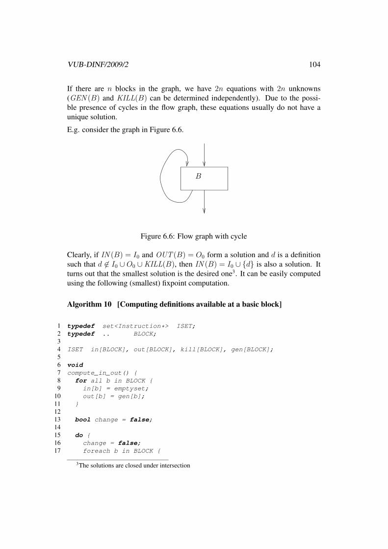
VUB-DINF/2009/2 104
If there are n blocks in the graph, we have 2n equations with 2n unknowns(GEN (B) and KILL(B) can be determined independently). Due to the possi-ble presence of cycles in the flow graph, these equations usually do not have aunique solution.
E.g. consider the graph in Figure 6.6.
B
Figure 6.6: Flow graph with cycle
Clearly, if IN (B) = I0 and OUT (B) = O0 form a solution and d is a definitionsuch that d 6∈ I0 ∪O0 ∪KILL(B), then IN (B) = I0 ∪ {d} is also a solution. Itturns out that the smallest solution is the desired one3. It can be easily computedusing the following (smallest) fixpoint computation.
Algorithm 10 [Computing definitions available at a basic block]
1 typedef set<Instruction*> ISET;2 typedef .. BLOCK;34 ISET in[BLOCK], out[BLOCK], kill[BLOCK], gen[BLOCK];56 void7 compute_in_out() {8 for all b in BLOCK {9 in[b] = emptyset;
10 out[b] = gen[b];11 }1213 bool change = false;1415 do {16 change = false;17 foreach b in BLOCK {
3The solutions are closed under intersection

VUB-DINF/2009/2 105
18 newin = set_union { out[c] | c < b };19 change = change || (newin != in[b]);20 in[b] = newin;21 out[b] = (in[b] - kill[b]) set_union gen[b]22 }23 while change;24 }25 }
2
Definition 20 Let a be a variable and let u be a point in the flow graph. The setof definitions of a that reach u is defined by
UD(a, u) = {d ∈ Def(a) | d reaches u}
Such a set is often called a use-definition chain.
UD(a, u) can be easily computed using IN (B) where u is the basic block con-taining u.
Algorithm 11 [Computing use-definition chains]
1 iset2 defu(SYM_INFO* a,POINT u) {3 BLOCK b = block_of(u);45 if (Def(a) intersection B != emptyset)6 /* return the singleton containing the last7 * definition in b of a before u8 */9 for (p=u; (p>0); --p)
10 if (p in UDEF(a))11 return {p}12 return Def(a) intersect in[b]13 }
2
6.3.2 Reaching definitions using datalog
An alternative definition uses logic programming (in particular, datalog) to definereaching definitions, see [ALSU07], page 925.

VUB-DINF/2009/2 106
We will use a term B.N, N ≥ 0 to denote the point in block B us before theN + 1’th statement (in block B). The latter statement is said to be at point B.N.We start with the following base predicates.
1 assign(B.N, X, E) % the statement following B.N has the2 % form X = E, E an expression (with at most 2 operands)3 use(B.N, X) % the statement at B.N uses the variable X4 type(X,T) % type type of X is T5 size(B, N) % block B has N statements6 succ(B, C) % true iff block B has a successor block C7 initial(B) :- not( succ(C,B) ). % initial block has no predecessors
We can then define what it means for a statement to (ambiguously or unam-bigously) define a variable X (here we assume a strongly typed language withoutcasting).
1 % unambig_def(B.N, X) -- statement N in block B unambiguously defines variable X2 unambig_def(B.N, X) :- assign(B.N, X, _).34 % def(B.N, X) -- statement N in block B may define variable X5 define(B.N, X) :- unambig_def(B.N, X).6 define(B.N, X) :- assign(B.N, *P, _), type(X, T), type(P, T*).
Then the following program computes the reaching definitions.1 % rd(B.N, C.M, X) -- definition of X at C.M reaches B.N2 rd(B.N, B.N, X) :- define(B.N, X).3 rd(B.N, C.M, X) :- rd(B.N-1, C.M, X), not(unambig_def(B.N-1, X)).4 rd(B.0, C.M, X) :- rd(D.N, C.M, X), succ(D, B), size(D,N).
The first rule simply states that a definition reaches itself while the second ruleindicates that if a definition reaches a point N − 1 in a block B and the nextstatement does not unambiguously (re)define X , then the definition also reachespointN (after the next statement) inB. The third rule says that a definition reachesthe beginning of a block B if it reaches the end of a predecessor D of B.
A use-definition predicate be defined as follows, where the use u is representedby a point N in a block B, and d by its block C and point M ):ud(A, u(B.N), d(C.M)) :- rd( B.N, C.M, A), use(B.N, A).
6.3.3 Available expressions
Definition 21 An expression e = x+y4 is available at a point p, denoted AVAIL(e, p)if every path from the initial basic block to p evaluates z = x + y, and after the
4We use ’+’ as an example operator. The same definition applies to other binary or unaryoperators.

VUB-DINF/2009/2 107
last such evaluation prior to p, there are no subsequent definitions for x, y or z.A block kills an expression x + y if it defines x or y and does not subsequently(re)compute x + y. A block generates an expression x + y is if it unambiguouslyevaluates x+ y and does not subsequently redefine x or y.
In order to be able to determine the availability of an expression at some point, wedefine
Definition 22 Let B be a basic block.
GEN e(B) = {e | B generates e}KILLe(B) = {e | B kills e}
IN e(B) = {e | e is available at the start of B}OUT e(B) = {e | e is available past the end of B}
Observe that GEN e(B), which depends only onB, is straightforward to constructusing a forward scan ofB, keeping track of available expressions by appropriatelyprocessing definitions. E.g. an instruction z = x + y makes x + y available butkills any available expressions involving z (note that z = x is possible). The setKILLe(B) consists of all expressions y+ z such that either y or z is defined in theblock and y + z is not generated by the block.
It is easy to see that IN e(B) and OUT e(B) must satisfy the following data-flowequations:
OUT e(B) = (IN (B) \KILLe(B)) ∪GEN e(B)
IN e(B) =
{∩C<BOUT e(C) if B is not initial∅ if B is initial
Note the similarity of these equations with the ones for reaching definitions. Themain difference is the use of ∩ instead of ∪ in the equation for IN e(B) (∩ isnecessary since e must be available on all paths into B in order to be sure that e isavailable at the start of B).
Consider the flow graph in Figure 6.7 and assume that neither x nor y are definedin block B after d which is itself the final definition of z in block B. Assumefurthermore that block C does not contain any definitions for x, y or z. Hencex + y should be available at the beginning of block C, i.e. x + y ∈ IN e(C),which would not be found if the minimal solution for the above equations werecomputed.
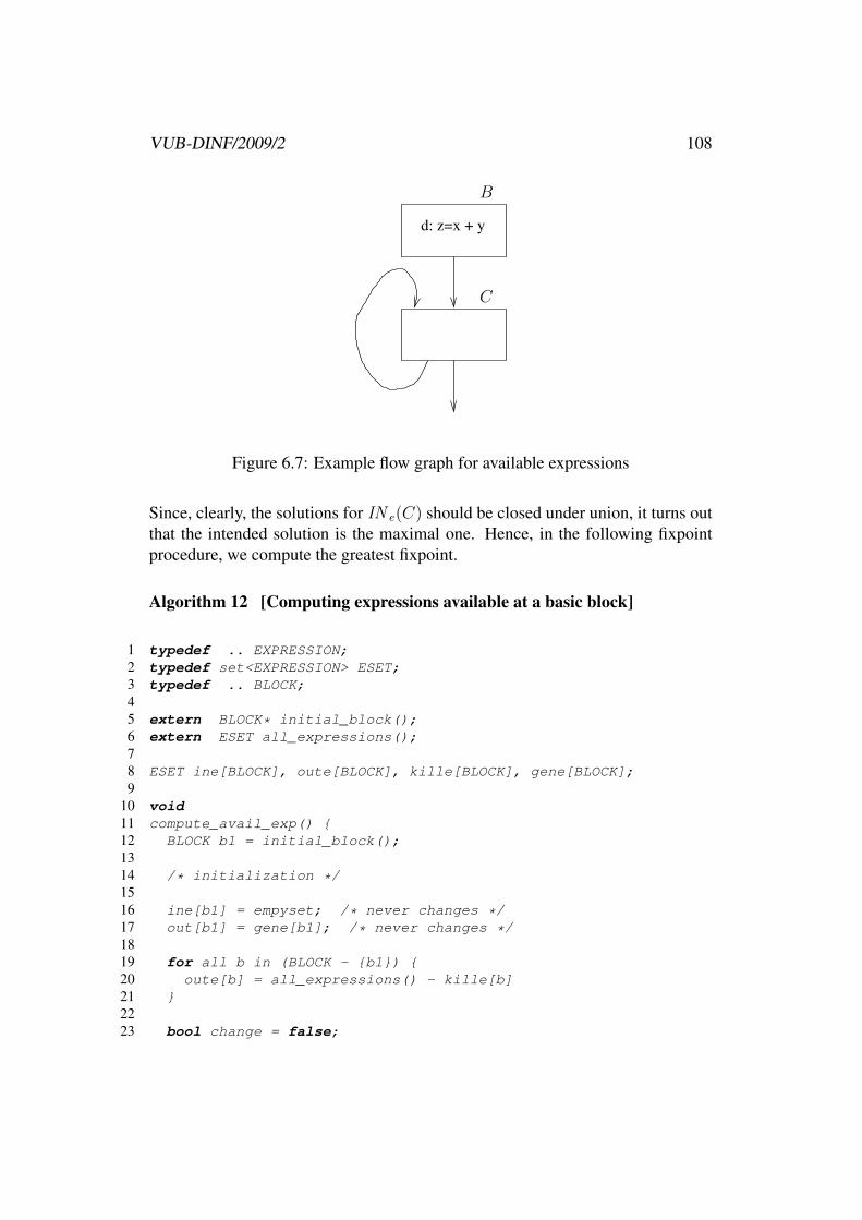
VUB-DINF/2009/2 108
d: z=x + y
B
C
Figure 6.7: Example flow graph for available expressions
Since, clearly, the solutions for IN e(C) should be closed under union, it turns outthat the intended solution is the maximal one. Hence, in the following fixpointprocedure, we compute the greatest fixpoint.
Algorithm 12 [Computing expressions available at a basic block]
1 typedef .. EXPRESSION;2 typedef set<EXPRESSION> ESET;3 typedef .. BLOCK;45 extern BLOCK* initial_block();6 extern ESET all_expressions();78 ESET ine[BLOCK], oute[BLOCK], kille[BLOCK], gene[BLOCK];9
10 void11 compute_avail_exp() {12 BLOCK b1 = initial_block();1314 /* initialization */1516 ine[b1] = empyset; /* never changes */17 out[b1] = gene[b1]; /* never changes */1819 for all b in (BLOCK - {b1}) {20 oute[b] = all_expressions() - kille[b]21 }2223 bool change = false;

VUB-DINF/2009/2 109
2425 do {26 change = false;27 for all b in (BLOCK - {b1}) {28 ine[b] = intersection { oute[c] | c < b }29 oldout = oute[b];30 oute[b] = gene[b] set_union (ine[b] - kille[b]);31 change = change || (oute[b]!=oldout);32 }33 }34 while (change);3536 }
2
Note that, based on IN e(B), it is easy to determine AVAIL(e = x + y, p), forp ∈ B.
Algorithm 13 [Computing expression availability at a point]Let p ∈ B be a point where we want to compute AVAIL(e, p).
• Check whether e ∈ IN e(B).
• If so, check whether x or y are redefined before p inB. If not, e is available;else not.
• If e 6∈ IN e(B), check whether e is generated before p in B. If so, e isavailable; else not.
2
6.3.4 Available expressions using datalog
In datalog, the formulation is slightly more involved than might be expected be-cause the usual datalog semantics computes minimal solutions. The approach isto define a predicate unavail_exp/2 asserting that an expression is not availableat some point. The availability of an expression at a point then hold is unavail
does not hold at that point.1 define_exp(B.N, X+Y) :- assign(B.N, _, X+Y).2 % a possibled definition of any operand kills the expression3 kill_exp(B.N, X+Y) :- define(B.N, X, _).4 kill_exp(B.N, X+Y) :- define(B.N, Y, _).

VUB-DINF/2009/2 110
56 unavail_exp(B.N, X+Y) :- kill_exp(B.N7 unavail_exp(B.N+1, X+Y) :-8 unavail_exp(B.N, X+Y), not(define_exp(B.N+1, X+Y)).9 % if X+Y is unavaible at the end of a predecessor of B,
10 % it is also unavailable at the beginning of B11 unavail_exp(B.0, X+Y) :- succ(C, B), size(C,N), unavail_exp(C.N, X+Y).12 % at the start of the initial block, all expressions are unavailable13 unavail_exp(B.0, X+Y) :- initial(B).14 % an expression is available if it is not unavailable15 avail(B.N, X+Y) :- not(unavail_exp(B.N, X+Y)).
6.3.5 Live variable analysis
Definition 23 A variable x is used at instruction s if its value may be required bys.
Definition 24 Let x be a variable and let p be a point in the flow graph. We saythat x is live at p is there is some path from p on which the value of x at p can beused. If x is not live at p, we say that it is dead at p.
In datalog this becomes:1 live(B.N, X) :- assign(B.N, _, X + Y).2 live(B.N, X) :- assign(B.N, _, Y + X).3 live(B.N-1, X) :- live(B.N, X),4 not(unambig_def(B.N-1, X).5 live(B.N, X) :- size(B, N), succ(B, C), live(C.0, X).
In order to be able to determine whether a variable is live at some point, we define
Definition 25 Let B be a basic block.
KILLlive(B) = {x | x is unambiguously defined before used in B}GEN live(B) = {x | x may be used in B before it is unambiguously defined in B}
IN live(B) = {x | x is live at the start of B}OUT live(B) = {x | x is live past the end of B}

VUB-DINF/2009/2 111
Note that, in the definition of KILLlive(B), it is not necessary that x is actuallyused in B, as long as there is an unambiguous definition of x before any use. Sim-ilarly, in the definition of IN live(B), it may well be that x ∈ IN live(B) although xis not (unambiguously) defined in B.
Observe that both KILLlive(B) and GEN live(B), which depend only on B, arestraightforward to construct.
To compute IN live(B) and OUT live(B), we note that they satisfy the followingdata-flow equations:
IN live(B) = GEN live(B) ∪ (OUT live(B)−KILLlive(B))
OUT live(B) = ∪B<CIN live(C)
Again we will use a fixpoint computation to determine the smallest solution of theabove equations. Note that intuitively, the algorithm works “backwards” in thegraph, as can be seen from the use of successors instead of predecessors in theequation for OUT live(B).
Algorithm 14 [Computing live variables for a basic block]
1 typedef set<SYM_INFO*> VSET;2 typedef .. BLOCK;34 VSET in_live[BLOCK], out_live[BLOCK], use[BLOCK], gen_live[BLOCK];56 void7 compute_live()8 {9 for all b in BLOCK
10 in_live[b] = emptyset;1112 bool change = true;1314 while (change) {15 change = false;16 foreach b in BLOCK {17 oldin = in_live[b];18 out_live[b] = union { in[s] | b < s };19 in_live[b] = use[b] union (out_live[b] - gen_live[b]);20 change = change || (oldin!=in_live[b]);21 }22 }23 }

VUB-DINF/2009/2 112
2
Note that the information from OUT live(B) can be profitably used to refine Al-gorithm 9.
6.3.6 Definition-use chaining
Definition 26 The definition-use chain of a definition d is defined as
DU (d, x) = {s | s uses x and there is a path from d to s that does not redefine x}
The following sets, defined for basic blocks, facilitate the computation of DU (d, x).
Definition 27 Let B be a basic block.
KILLuse(B) = {(s, x) | s 6∈ B uses x and B defines x}GEN use(B) = {(s, x) | s ∈ B uses x and x is not defined prior to s in B}
IN use(B) = {(s, x) | s uses x and s reachable from the beginning of B}OUT use(B) = {(s, x) | s 6∈ B uses x and s reachable from the end of B}
Here, “reachable” means without any intervening definitions of x.
Observe that both KILLuse(B) and GEN use(B) are straightforward to construct.
To compute IN use(B) and OUT use(B), we note that they satisfy the followingdata-flow equations:
IN use(B) = GEN use(B) ∪ (OUT use(B)−KILLuse(B))
OUT use(B) = ∪B<CIN use(C)
Since the above equations are isomorphic to the ones in Section 6.3.5, an algo-rithm similar to Algorithm 14 can be used to compute OUT use(B). DU (d, x) canthen be computed by.
DU (d, x) =
OUT use(B) ∪ {(s, x) | s ∈ B uses x}
if B does not contain a definition of x after d{(s, x) | s ∈ B uses x and s comes before d′}
if d′ ∈ B is the first definition of x after d

VUB-DINF/2009/2 113
6.3.7 Application: uninitialized variables
To illustrate the use of global flow information, we show how to detect uninitial-ized variables.
It suffices to add a dummy assignment dx:x = 0 for each variable x in front of theinitial block. Now if for any such dx, it turns out that DU (dx, x) 6= ∅, we candeduce that x is possibly used before it is assigned to.
6.4 Global optimization
6.4.1 Elimination of global common subexpressions
Algorithm 15 [Elimination of global common subexpressions]For every instruction s:x = y+z5 such that AVAIL(y+z, p) where p is the pointbefore s, do the following (assume s ∈ B):
1. Find the evaluations of y+z that reach B by searching the graph (and eachblock) backwards from B, not continuing after a block that evaluates y+ z.
2. Create a new temporary variable u.
3. Replace each instruction w = y + z found in step 1 by u = y + z;w = u.
4. Replace s by x = u.
2
Note that the algorithm will miss the fact that a ∗ z is the same as c ∗ z in
1 a = x + y2 b = a * z3 ...4 c = x + y5 d = c * z
Figure 6.8: Code before first subexpression elimination
Algorithm 15 will produce the code in Figure 6.9. However, repeated applicationof Algorithm 15, combined with copy propagation (Algorithm 16), will eventuallyoptimize the code further.
5Here ’+’ stands for any operator.

VUB-DINF/2009/2 114
1 u = x + y2 a = u3 b = a * z4 ...5 c = u6 d = c * z
Figure 6.9: Code after first subexpression elimination
6.4.2 Copy propagation
Copy instructions of the form x = y are generated e.g. by intermediate codegeneration and by Algorithm 15. Copy propagation can be used to eliminate manysuch instructions by replacing further uses of x by y.
One can eliminate a copy instruction s:x = y and substitute y for x in all uses ofx in s′ ∈ DU (s, x) provided that:
• UD(s′, x) = {s}, i.e. s is the only definition of x to reach s′.
• No paths from s to s′, including paths that go through s′ several times,contains definitions of y.
In datalog:1 % copy(B.N, X, Y) -- X is copy of Y at B.N2 copy(B.N, X, Y) :- assign(B.N, X, Y).3 copy(B.N, X, Y) :- copy(B.N-1, X, Y),4 not( def(B.N-1, X) ), not( def(B.N-1, Y) ).5 copy(B.0, X, Y) :- not( initial(B) ),6 not (7 succ(C, B), size(C, M), not( copy(C.M, X, Y) )8 ).
To solve the latter question, we solve yet another data-flow problem where IN copy(B)(OUT copy(B)) is the set of copies s : x = y such that every path from the initialnode to the beginning (end) of B contains s, and subsequent to the last occurrenceof s, there are no definitions of y. We also consider GEN copy(B), the set of copiess:x = y generated by B where s ∈ B and there are no subsequent definitions ofx or y within B. KILLcopy(B) contains the set of copies s:x = y where either xor y is defined in B and s 6∈ B. Note that IN copy(B) can contain only one copyinstruction with x on the left since, otherwise, both instructions would kill eachother.

VUB-DINF/2009/2 115
Then the following equations hold:
OUT copy(B) = GEN copy(B) ∪ (IN copy(B) \KILLcopy(B))
IN copy(B) =
{∩C<BOUT copy(C) if B is not initial∅ if B is initial
Note that these equations are isomorphic to the ones used for Algorithm 12 andtherefore we can use a similar algorithm to solve them.
Given IN copy(B), i.e. the set of copies x = y that reach B along every path, withno definition of x or y following the last occurrence of x = y on the path, we canpropagate copies as follows.
Algorithm 16 [Copy propagation]For each copy instruction s:x = y do the following:
1. Determine DU (s, x), i.e. the set of uses s′ that are reached by s.
2. Check whether for every s′ ∈ DU (s, x), s ∈ IN copy(Bs′)6, i.e. s reaches
Bs′ on every path and, moreover, no definitions of x or y occur prior to s′
in B.
3. If the previous step succeeds, remove s and replace x by y in each s′ ∈ DU (s, x).
2
Applying Algorithm 16 on the code of Figure 6.9 yields1 u = x + y2 b = u * z3 ...4 d = u * z
Now, running Algorithm 15 again will result in1 u = x + y2 v = u * z3 b = v4 ...5 d = v
6Bs′ is the basic block containing s′.

VUB-DINF/2009/2 116
6.4.3 Constant folding and elimination of useless variables
Another transformation concerns the propagation of constants. As an example,consider the code
1 t0 = 332 t1 = 33 t2 = t0 + t14 t3 = t2 - 355 x = t3;
Algorithm 17 [Constant folding]Call a definition s:x = a+ b7 “constant” if all its operands a and b are constant.
• We can then replace s by x = c where c = a+ b is a new constant.
• For each constant definition s and for each s′ ∈ DU (x, s), if UD(x, s′) = {s},i.e. s is the only x-definition reaching s′, we can replace x in s′ by c, possi-bly making s′ constant. If after this, DU (x, s) = ∅, we can eliminate s.
• Repeat the above steps until there are no further changes.
2
Note that the second step above can be seen as a special simple case of copypropagation since the right hand side c of the copy instruction x = c is constantand therefore there are no c-assignments to worry about.
In the example, application of the algorithm sketched above yields1 x = 1
6.4.4 Loops
It is a well-known piece of computer science folklore that programs tend to spend90% of their execution time in 10% of their code. One can use a profiling toolsuch as gprof to collect statistics on a program run from which it can be deducedwhich routines and instructions are most often executed. These “hot spots” willalmost always turn out to be loops. So it is natural to concentrate optimizationefforts on loops.
Before considering loop optimization, we need to define what constitutes a loopin a flow graph.
7Here + may be any operator.
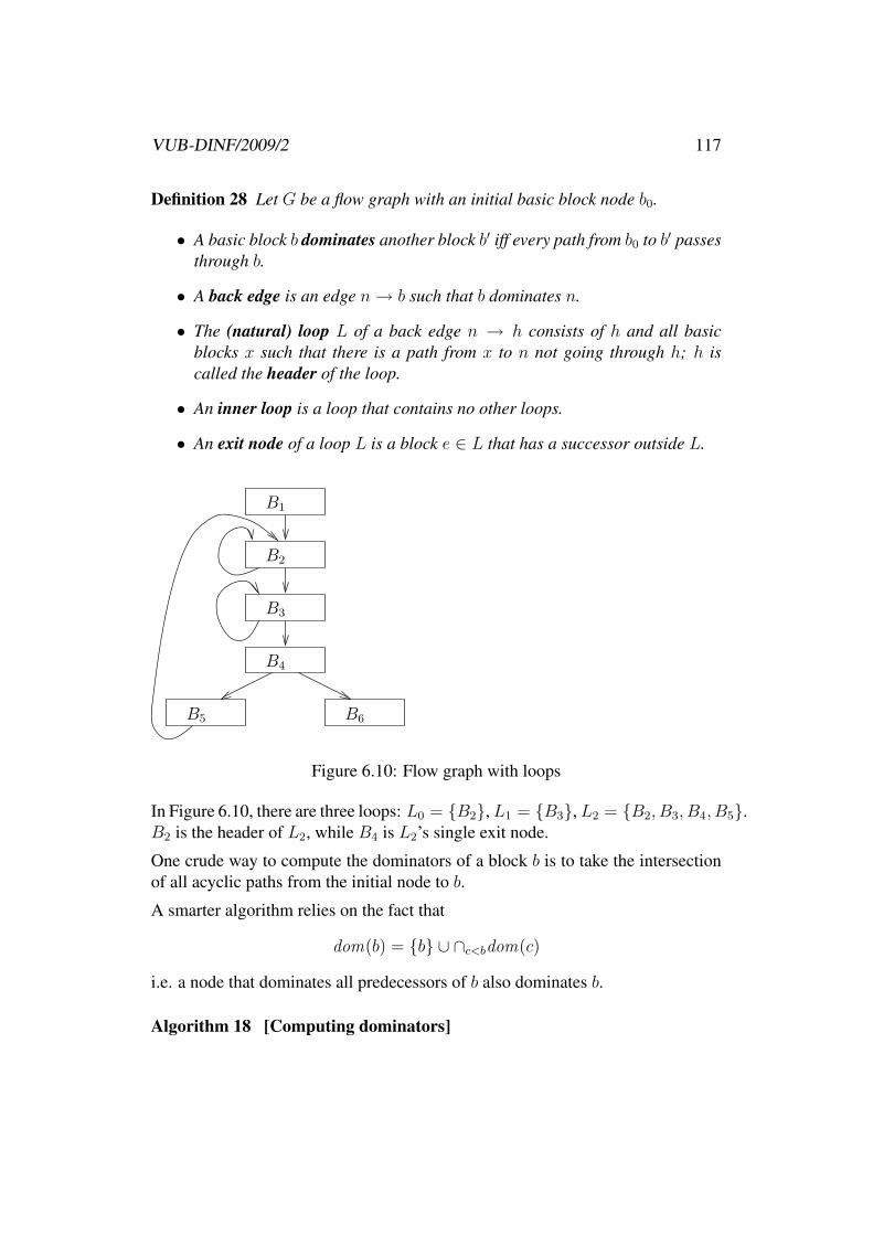
VUB-DINF/2009/2 117
Definition 28 Let G be a flow graph with an initial basic block node b0.
• A basic block b dominates another block b′ iff every path from b0 to b′ passesthrough b.
• A back edge is an edge n→ b such that b dominates n.
• The (natural) loop L of a back edge n → h consists of h and all basicblocks x such that there is a path from x to n not going through h; h iscalled the header of the loop.
• An inner loop is a loop that contains no other loops.
• An exit node of a loop L is a block e ∈ L that has a successor outside L.
B1
B2
B3
B6B5
B4
Figure 6.10: Flow graph with loops
In Figure 6.10, there are three loops: L0 = {B2}, L1 = {B3}, L2 = {B2, B3, B4, B5}.B2 is the header of L2, while B4 is L2’s single exit node.
One crude way to compute the dominators of a block b is to take the intersectionof all acyclic paths from the initial node to b.
A smarter algorithm relies on the fact that
dom(b) = {b} ∪ ∩c<bdom(c)
i.e. a node that dominates all predecessors of b also dominates b.
Algorithm 18 [Computing dominators]

VUB-DINF/2009/2 118
1 typedef set<BLOCK*> BLOCKS;23 BLOCK* b0; /* initial basic block */4 set<BLOCK*> B; /* set of all blocks */56 void7 compute_dominates()8 {9 /* initialize */
1011 dom(b0) = { b0 };12 for b in (B - {b0})13 dom(b) = B;1415 /* compute fixpoint */1617 do18 {19 change = false;20 for b in (B-{b0})21 {22 old_dom = dom(b);23 dom(b) = {b} union intersection { dom(c) | c < b }24 change = change || (dom(b)!=old_dom);25 }26 }27 while (change)28 }
2
The table below shows the application of Algorithm 19 to the flow graph of Fig-ure 6.10.
block 1 2 3 4 5 6predecessors 1,2,5 2,3 3 4 4dominators initialize 1 1,2,3,4,5,6 1,2,3,4,5,6 1,2,3,4,5,6 1,2,3,4,5,6 1,2,3,4,5,6dominators iteration 1 1 1,2 1,2,3 1,2,3,4 1,2,3,4,5 1,2,3,4,6dominators iteration 2 1 1,2 1,2,3 1,2,3,4 1,2,3,4,5 1,2,3,4,6
The following algorithm can be used to compute the natural loop correspondingto a back edge. It corresponds to a backward scan from the header.
Algorithm 19 [Computing the natural loop of a back edge]

VUB-DINF/2009/2 119
1 type set<BLOCK*> BLOCKS;23 typedef struct {4 BLOCKS nodes;5 BLOCK* header;6 } LOOP;78 BLOCKS9 predecessors(BLOCK *b); /* return predecessors of b in flow graph */
1011 LOOP12 natural_loop(BLOCK* src,BLOCK* trg)13 {14 /* compute natural loop corresponding to back edge src-->trg */1516 BLOCK* stack[];17 BLOCK* tos = stack;18 LOOP loop = { { trg }, trg }; /* trg is header */1920 if (trg!=src) {21 loop.nodes = loop.nodes union { src }22 stack[tos++] = src; /* push src */23 }2425 while (tos!=stack) { /* stack not empty */26 BLOCK* b = stack[--tos]; /* pop b */27 BLOCKS P = predecessors(b);2829 for each p in P30 if (!(p in loop)) {31 loop.nodes = loop.nodes union {p};32 stack[tos++] = p;33 }3435 }36 }
2
Applying Algorithm 19 to the back edgeB5 → B2 in the flow graph of Figure 6.10is illustrated in the table below.
faze loop.nodes stackinitialize {2}adding src {2, 5} 5iteration 1 {2, 5, 4} 4iteration 2 {2, 5, 4, 3} 3iteration 3 {2, 5, 4, 3}

VUB-DINF/2009/2 120
6.4.5 Moving loop invariants
A loop invariant is a instruction of the form s:x = y + z8 such that x does notchange as long as control stays in the loop. Such instructions can, under certainconditions, be moved outside of the loop so that the value x is computed onlyonce.
Example 20 Consider a C function to compute the scalar product of two vectors(represented as arrays).
1 int2 innerproduct(int a[]; int b[], int s) {3 // s is size of arrays4 int r = 0;5 int i = 0;6 while (i<s) {7 r = r + a[i]*b[i];8 i = i+1;9 }
10 return r;11 }
The flow graph, after code simplification, is shown in Figure 6.11 on page 121.Note that the size of an int is assumed to be 4 bytes, as witnessed by the offsetcomputation t1 = 4* i.
Applying Algorithm 19 on the graph of Figure 6.11 yields that, among others, Cdominates A, B and D and that, consequently, D → C is a back edge. It thenfollows from Algorithm 19 that L = {D,C} is an inner loop with exit node C.
Algorithm 20 [Computing loop invariants]Given a loop L, we find the list of loop invariants from L as follows (note that
the order of the list is important, as it reflects the order of the instructions afterhaving been moved):
1. Mark “invariant” (and append to the list of invariants) all instructionss:x = y + z such that each operand y (or z) is either constant or is suchthat UD(y, s) ∩ L = ∅, i.e. all its reaching definitions are outside L.
2. Repeat the following step until no more instructions are marked.
3. Mark (and append to the list) “invariant” all instructions s:x = y + z suchthat each operand y (or z) is
8Here + stands for any operator.

VUB-DINF/2009/2 121
r = 0
i = 0
E
C
B
A
D t1 = 4 * i
if i<s goto B
goto A
return r
t2 = &a
t3 = t2[t1]
t4 = &b
t5 = t4[t1]
t6 = t3 * t5r = r + t6
i = i+1
goto C
Figure 6.11: Flow graph of Example 20
• constant; or
• all its reaching definitions are outside L; or
• UD(y, s) = {q} where q ∈ L is marked invariant; i.e. the only reach-ing definition of y is an invariant in the loop.
2
Applying Algorithm 20 for Example 20 yields two loop invariants: t2 = &a andt4 = &b, both in block D.
Having found the invariants in a loop, we can move some of them outside theloop. They will be put in a new node, called a preheader which has as its singlesuccessor the header of the loop. The flow graph is further updated such that alledges that pointed from outside the loop to the header, will be made to point tothe new preheader node.
Algorithm 21 [Moving invariants]Let I be the list of invariants of the loop L.
1. For each s:x = y + z from I , check that:

VUB-DINF/2009/2 122
(a) s is in a block b that dominates all exits of L or x 6∈ IN live(e) for anysuccessor e 6∈ L of an exit block of L; and
(b) x is not defined anywhere else in L; and
(c) For each use s′ of x in L, UD(x, s′) ∩ L = {s}, i.e. all uses of x in Lcan only be reached by the definition s of x
2. Move instructions from I that satisfy the above test, and that do not dependon definitions in I that do not pass the test, to the preheader, in the sameorder as they appear in I .
2
Figure 6.12 shows the result of applying Algorithm 21 to Example 20. Note thatthe block (D) containing t2 = &a does not dominate all exits of L. However,since t2 6∈ IN live(B), condition (1a) above is still satisfied.
C
B
A
D t1 = 4 * igoto A
return r
r = 0
i = 0
E
t2 = &a
t4 = &b
t3 = t2[t1]
t5 = t4[t1]
t6 = t3 * t5
r = r + t6
i = i+1
goto C
H
if i<s goto D
Figure 6.12: Flow graph of Example 20 after moving loop invariants

VUB-DINF/2009/2 123
6.4.6 Loop induction variables
A variable x is called an induction variable of a loop L if every time it changesvalue, it is incremented or decremented by some constant. Examples include arrayindexes that are incremented on each pass through the loop, counters correspond-ing to for instructions etc.
Often, one induction variable depends on another one.
E.g. in Example 20, both i and t1 are induction variables where t1 depends oni.
Definition 29 Let L be a loop. A basic induction variable is a variable i suchthat the only assignments to i in L are of the form i = i± c where c is a constant.An induction variable is a variable j such that j is defined only once in L and itsvalue is a linear function of some basic induction variable i, i.e. j = a × i + bfor some constants a, b. We say that j belongs to the family of i, and associate thetriple (i, a, b) with j.
The following algorithm determines the induction variables of a loop.
Algorithm 22 [Finding the induction variables of a loop]Given a loop L, we proceed as follows:
1. Find all basic induction variables i. Such variables are associated with thetriple (i, 1, 0).
2. Find variables k such that Def(k) ∩ L is a singleton s which has one ofthe forms k = j × b, k = b× j, k = j/b, k = b/j, k = j ± b, or k = b± j,where b is a constant and j is an induction variable, basic or otherwise.
• If j is basic, then k is in the family of j and we associate k with theappropriate triple. E.g. if s:k = j × b then the triple of k is (i, b, 0).
• If j is not basic, then j belongs to the family of some basic inductionvariable i. We first check the following additional conditions:
– There is no definition of i between the (single) definition of j in Land the (single) definition of k; and
– (UD(j, s) \ L) = ∅, i.e. no definition of j outside L reaches s.
Provided these conditions are met, we add k to the family of i andassociate it with the triple (i, b× c, b× d), where we assume that s isof the form k = j × b and the triple of j is (i, c, d).

VUB-DINF/2009/2 124
2
Applying Algorithm 22 to the loop L = {C,D} in Figure 6.12 yields:
• a basic induction variable i which is associated with the tuple (i, 1, 0).
• an induction variable t1 in the family of i. t1 is associated with the tuple(i, 4, 0).
Once we have found suitable induction variables, we can perform strength reduc-tion, where expensive multiplications are replaced by cheaper additions, as in thefollowing algorithm
Algorithm 23 [Strength reduction]Given a loop L and a set of induction variables, each with associated triple, we
consider each basic induction variable i in turn.For each non-basic induction variable j with associated triple (i, c, d) we do thefollowing:
1. Create a new variable t (but if two variables j1 and j2 have the same triples,create only one variable for both of them).
2. Replace the unique assignment to j in L by j = t.
3. Immediately after each assignment i = i+ a (a constant) to the basic in-duction variable i in L, add an instruction t = t+ c× a and place t in thefamily of i with triple (i, c, d).
4. To properly initialize t, put
t = c× it = t+ d
at the end of the preheader of L.
2
The result of applying Algorithm 23 to the loop L = {C,D} in Figure 6.12 isshown in Figure 6.13.
Block D can be further simplified using Algorithm 9 (code simplification): be-cause t1 6∈ OUT live(D), t1 will be eliminated. On the other hand, block Bcan be simplified using copy propagation and constant folding (Algorithms 16and 17). The result is shown in Figure 6.14.
After strength reduction, it may be that the only use of some induction variable iis in tests such as

VUB-DINF/2009/2 125
C
B
A
Dgoto A
return r
t1 = t
t3 = t2[t1]
t5 = t4[t1]
t6 = t3 * t5
i = i+1
r = r + t6
goto C
t = t + 4
t = 4 * i
t = t + 0
t2 = &a
t4 = &b
r = 0
i = 0
E
H
if i<s goto D
Figure 6.13: Flow graph of Example 20 after strength reduction
1 if i>C goto XXX
(and in the computation of other induction variables). In such a case, it may beprofitable to replace the variable in the test by another induction variable j fromthe same family, and modify the test accordingly.
E.g., in our example (Figure 6.14), the triple of t is (i, 4, 0), and we can replacethe code in block C by
1 s1 = 4 * s2 if t<s1 goto B
After this it may become possible to eliminate i since it is only used to computeitself. It may also be that the definition of the new temporary corresponds to aloop invariant which may be moved outside the loop.

VUB-DINF/2009/2 126
C
B
A
Dgoto A
return r
goto C
t = t + 4
t2 = &a
r = 0
i = 0
E
H
t = 0
t4 = &b
t3 = t2[t]
t5 = t4[t]
t6 = t3 * t5
r = r + t6
i = i+1
if i<s goto D
Figure 6.14: Flow graph of Figure 6.13 after copy propagation and constant fold-ing
A more detailed description of this algorithm can be found in [ASU86].
Applying the above transformations to Example 20 results in the final graph de-picted in Figure 6.15.
6.5 Aliasing: pointers and procedure calls
Two expressions are aliases of each other if they denote the same memory address.Both pointers and procedure calls introduce aliases. Aliases complicate data-flowanalysis and code improvement, locally (see e.g. Section 6.2.3, page 100) as wellas globally.

VUB-DINF/2009/2 127
C
B
A
Dgoto A
return r
goto C
E
H
t3 = t2[t]
t5 = t4[t]
s1 = 4 * s
t = 0
t4 = &b
t2 = &a
r = 0
r = r + t6
t6 = t3 * t5
t = t + 4
if t<s1 goto D
Figure 6.15: optimized flow graph for Example 20
If nothing is known about where a pointer points to, as is e.g. the case in a lib-eral language such as C, we must assume that any pointer assignment ∗p = e canpotentially define any variable. Likewise, dereferencing a pointer, as in x = ∗pmust be counted as a use of any variable. This obviously increases the number oflive variables and reaching definition, while decreasing the number of availableexpressions. The net result is fewer code improvement opportunities.
A similar reasoning holds for procedure calls: if nothing is known about whichvariables the procedure may change, we must assume that it potentially defines allvariables.
If, e.g. because of the rules of the source language, we know more about thepossible usage of pointers and/or procedure calls, we may improve matters.

VUB-DINF/2009/2 128
6.5.1 Pointers
We deal with pointers first. For each basic block B, we define two sets IN ptr(B)and OUT ptr(B) containing pairs (p, a) where p is a pointer variable and a isanother variable. Intuitively, (p, a) ∈ IN ptr(B) means that, on entry to B, p maypoint to a (note that there may be several a such that (p, a) ∈ IN ptr(B)), whileOUT ptr(B) encodes where pointers may point upon exit of B.
The knowledge about pointer rules is encoded in a set of functions transs, one foreach type of instruction s, which transforms a set of pairs (p, a) into another suchset which is such that, if p may point to any a such that (p, a) ∈ S, then, after s, pmay point to any b such that (p, b) ∈ transs(S). transs can be extended to transBfor any basic block B by composing , in order, the functions corresponding to theinstructions of B. IN ptr(B) and OUT ptr(B) then satisfy the data-flow equations.
OUT ptr(B) = transB(IN ptr(B))
IN (B) = ∪C<BOUT ptr(B)
Note that these equations are isomorphic to the ones used to compute reaching def-initions (Section 6.3.1, page 103, and hence one can use Algorithm 10 (page 104)to compute the smallest fixpoint.
IN ptr(B) can then be used to derive a precise set of variables that may be definedby an instruction such as ∗p = e. Similarly, the set of variables that may be usedby an instruction such as a = ∗p can be derived from IN ptr(B), and the data-flowalgorithms can be suitably refined to take this information into account (note that,e.g. for use-definition chains, unless p can point to only one variable, we must notconsider ∗p = a as a definition that may hide earlier ones).
6.5.2 Procedures
If we have knowledge about procedures, we can apply a similar reasoning as forpointers in order to better estimate the effect of CALL instructions. In this section,we will use p(&x, y) to denote a procedure calling sequence in three address codewhere x is passed by reference while y is not.
As an example, we consider the case of C where procedures may only modifylocal and global variables. Note that procedures may also pass global variablesas reference parameters9. Clearly, passing a variable x for a reference formal
9In C, reference parameters are simulated by passing a pointer by value.

VUB-DINF/2009/2 129
parameter y makes x and y aliases, denoted x ≡ y (we assume that the names ofall local variables, including formal parameters, in all procedures and the namesof global variables are all distinct).
The following algorithm computes the set of possible aliases amongst all vari-ables.
Algorithm 24 [Computing aliases]We show only reference formal parameters for the procedures.
1. For each procedure p(&x1, . . . ,&xn) and each call p(&y1, . . . ,&yn), addx1 ≡ y1, . . . , xn ≡ yn to the set of aliases.
2. Take the reflexive and transitive closure of the relation ≡ resulting fromstep 1.
2
Now we can determine the set change(p), where p is a procedure, of global vari-ables and formal parameters10 that may possibly be changed by a call to p.
Define
• def (p) as the set of formal parameters and globals of p that have definitionsin the flow graph of p.
• Ap as the set of global variables or formal parameters a of p such that pcontains a call q(. . . ,&a, . . .) and the corresponding formal parameter is inchange(q).
• Gp as the set of global variables in change(q) where p calls q.
Thenchange(p) = def (p) ∪ Ap ∪Gp
and this equation can be solved by a smallest fixpoint computation, starting withchange(p) = def (p) as an underestimate.
change(p) can then be used as an estimate of possible definitions of variables,e.g. when computing available expressions (see also Section 10.8 in [ASU86]). Asimilar analysis can be made for the possible uses represented by a procedure call(for local variables this is easy: they are at most the parameters, for globals, onewould need to analyze the call graph of the called procedure).
10Note that formal parameters of p are also local variables of p.
Chapter 7
Code generation
Code generation concerns the generation of machine code from (relatively) machine-independent intermediate code.
Actually, there are a few possibilities as to exactly what kind of “machine code”is generated:
• One could generate so-called absolute machine code in which addresses arefixed (“absolute”) as much as possible. This strategy predates multiprocess-ing operating systems and was of little use in modern operating systems.It may however be relevant again in the context of so-called “just-in-time”compilers.
• It is also feasible to generated relocatable code where most addresses arerelative to some unknown base addresses. The code then has to be processedby a linker-loader before it can be executed. Since this option duplicates thework done by an assembler, we prefer the next option.
• We generate assembler source code where addresses are symbolic and leaveit to a separate program to translate further to relocatable code.
Code generation deals mainly with the following issues:
• Run-time storage management is concerned with the mapping of names toaddresses. We will look mainly at stack-based allocation of local variablesinto so-called activation records.
• Instruction selection. Depending on the characteristics of the hardware andthe context, the same instruction may be translated in several ways, eachwith different costs in time and/or space.
130

VUB-DINF/2009/2 131
• Closely related to the previous concern is the issue of register allocation.Many processors have very efficient instructions that take their operandsfrom a limited set of registers. The aim is to allocate registers to variablesin order to optimize global performance.
7.1 Run-time storage management
7.1.1 Global data
The global memory layout for a traditional language such as C is shown in Fig-ure 7.1. Of course, in modern operating systems, these areas may be in differentmemory segments, with different permissions, e.g. the code segment may be read-only and shared.
Code
StaticData
Stack
Heap
Figure 7.1: Memory layout in C
For static global variables, there is usually no problem: we simply use assemblerpseudo-operations like
1 GLOBAL BYTE 4,0 ; allocate & initialize 4 byte quantity GLOBAL
For dynamic global variables (e.g. the new operator in C++), memory is (de)allocatedat run-time from a so-called heap. Efficient algorithms for heap management, in-cluding e.g. garbage collection, are outside the scope of this text.

VUB-DINF/2009/2 132
7.1.2 Stack-based local data
If we are dealing with a language such as C, we also have to provide storage forlocal variables. If the language supports recursion, we are naturally lead to astack-based organization where, upon a function/procedure call, a so-called acti-vation record is pushed onto the stack. Upon return from the call, the activationrecord is popped.
A possible layout for an activation record is shown in Figure 7.2.
temporaries
temporaries
returned value
parameters
returned value
parameters
links and saved statusSP
caller’sresponsibility
callee’sresponsibility
activationrecordlinks and saved status
local data and
local data and
Figure 7.2: Activation records
Such a record contains, in growing stack order,
• Room for the value to be returned by the procedure (if any).
• The actual parameters.
• Links and saved status. The first item here is the stack pointer to be restoredupon exit of the procedure. The next one might be the return address, i.e. the

VUB-DINF/2009/2 133
address to which control should be transferred upon exit of the procedure.There may be additional hardware status information that is save here forrestoration upon exit of the call.
• Room for local and temporary variables. By local variables, we mean theones explicitly declared by the programmer. Temporary variables have beengenerated by the compiler during intermediate code generation and/or opti-mization.
The above organization is convenient because it allows an easy division of thework between caller and callee. The scenario for a procedure call is:
1. The caller evaluates the actual parameters and pushes them on the stack(note that the caller knows where is the top of the stack, since it knows SPand the size of its local and temporary data).
2. The caller pushes the value of SP, followed by the return address. It thenputs SP to its new value and transfers control to the callee, e.g. by a jumpinstruction.
3. The callee saves further status information on the stack (using SP). Thecallee may further update SP to point just past the saved information (as inthe figure).
4. The callee initializes its local data and goes about its further business.
A possible return (from a call) sequence is:
1. The callee places the return value is the appropriate place (note that it knowshow many and which parameters it received, so the return value will bestored at SP [−c] for some known c).
2. The callee restores the saved information, including the SP and jumps to thesaved return address.
3. The caller has access to the returned value (right at the top of the stack),which it may copy into its local data.
It should be clear that, at run time, a register will be used to store SP. Access tolocal data will then be achieved using indirect addressing through the contents ofSP and some constant offset which is known at compile time. This offset can eas-ily be computed and stored in the symbol table. An interesting aspect is that localvariables or temporaries may share a slot in the activation record provided theyare never live at the same time. This occurs, e.g. when compiling the following Ccode.

VUB-DINF/2009/2 134
1 int f(int x)2 {3 int a, b; /* slot 0, 1 */45 ...67 if (x>1) {8 int y; /* slot 2 */9
10 ...11 }12 else {13 int z; /* slot 2 */14 }15 }
In the example, y and z will never be alive at the same time since they are indifferent (non-nested) scopes. Therefore, both can share slot 2.
Note also that the organization above leaves the possibility for a procedure to havelocal data whose size is only known at run-time. E.g. variable-sized arrays canbe allocated on top of the stack, with a pointer to them reserved in the fixed-sizelocal data area.
7.2 Instruction selection
Even abstracting from the register allocation program (Section 7.3, page 136),there may be several possibilities and constraints involved in the translation of anintermediate code instruction.
As a simple example, consider the intermediate code instruction1 a = a + 1
This may be translated as (note the use of indirect addressing to access localnames):
1 load [sp]+a,r0 ; copy a to register 02 add #13 store r0,[sp]+a ; copy register 0 back to a
but if the processor supports an inc (increment) instruction, it could also be trans-lated as
1 inc [sp]+a ; increment a

VUB-DINF/2009/2 135
Some operations may only be possible with certain registers. E.g. on the IBM/370architecture, multiplication needs to performed as shown in Figure 7.3, i.e. oneoperand must be available in the odd register of an even-odd register pair whichwill be filled with the result.
r0 r1a
bB
r0 r1
mul r0,B
a × b
Figure 7.3: Multiplication on IBM/370
Addressing modes also influence the cost of an instruction. As an example, sup-pose the following table gives addressing modes and (relative) costs.
move r0,r1 1 register-to-registermove [r0],[r1] 1 register-to-register (indirect)move r5,x 2 register-to-memorymove #1,r3 2 constant-to-registermove [r0]+4,[r1]+5 3 indexed-to-indexed
We can then consider the following alternative code sequences for a = b+ c (as-suming they are all global):
• We can use a scratch register (total cost 6):1 move b,r02 add c,r0 ; result in r03 move r0,a
• We can perform addition in “memory” (total cost 6):1 move b,a2 add c,a
• If the values of b and c are in registers r1 and r2, we can reduce the cost to3, provided that b is not live after the instruction:

VUB-DINF/2009/2 136
1 add r2,r12 move r1,a
As the example illustrates, register allocation can have a dramatic effect on per-formance.
7.3 Register allocation
We describe how register allocation can be reduced to a graph coloring problem.
The idea is that, for a given flow graph (procedure), every variable corresponds toa symbolic register 1. The problem then is to assign each of a limited number ofreal registers to symbolic ones without introducing errors.
Clearly, we cannot use the same real register for symbolic registers (variables) r1
and r2 if e.g. r1 is defined at a time when r2 is live.
Definition 30 The register inference graph G corresponding to a flow graph isan undirected graph where the nodes are the symbolic registers and there is anedge between r1 and r2 is r1 is defined at a point where r2 is live.
If there are k real registers available, every symbolic register can be mapped to areal one without causing errors if G can be colored using k colors (no connectednodes may have the same color). Graph coloring with k colors is known to beNP-complete if k > 2 but the following heuristic procedure gives good results inpractice.
Algorithm 25 [Register allocation using graph coloring]Let G be the graph to be colored.
1. While there is a node n with fewer than k connected edges, remove the n(and remember it).The reason for this is that n can always receive a color, independent of thecolor chosen for its neighbors.
2. If we are left with an empty graph, G was colorable and we can assigncolors by coloring the nodes in the reverse order (of removal).
1The algorithm can be adapted to hardware peculiarities where, e.g., a special register needs tobe used for certain instructions. In this case, we associate a symbolic register with these instruc-tions; the register is defined at the time the instruction is used.

VUB-DINF/2009/2 137
3. If we are left with a nonempty graph, it is not k-colorable since it has a nodewith at least k neighbors. We then choose a node n to be spilled, removethe node from the graph and start again with step 1. Spilling a node meansthat the corresponding variable will be loaded (into a register) on each useand stored back on each definition.
Several heuristics have been proposed to choose a spilled node:
• Choose a node with a maximal number of attached edges, maximizing thechance of ending up with a k-colorable graph.
• Estimate the cost of spilling a node, and choose the one with the lowestcost. A simple measure would count the number of extra load/store instruc-tions, taking care to multiply with a suitable factor any such instructionsthat appear in a loop2.
2
7.4 Peephole optimization
Some machine code optimizations are very easy to perform by scanning the code(using a sliding window of instructions, hence the name) for certain patterns thatcan be replaced by improved patterns.
Often, it is the case that successful replacements induce opportunities for furtherreplacements; therefore scanning is usually repeated until no further matches arefound.
Below we list some example patterns and replacements.
2One could also have a higher cost factor for instructions in an inner loop than in an encom-passing loop.

VUB-DINF/2009/2 138
Pattern Replacement Descriptionmove x,y move x,y redundant load, storemove y,xjump(con) z jump(notcon) y jumps over jumpsjump y z: (seq1)z: (seq1) y: (seq2)y: (seq2)jump(con) z jump(con) y jumps to jumps.. ..z: jump y z: jump ymul #1,x (delete) algebraicadd #0,x (delete) simplificationmul #2,x add x,x machine specificsmul #2,x shiftleft x,1 machine specificsadd #1,x inc x machine specifics

Appendix A
A Short Introduction to x86Assembler Programming underLinux
A.1 Architecture
Memory is byte addressable. There are several general purpose registers: %eax,%ebx, %ecx, %edx, %edi and %esi.
The following registers have a special purpose:
• The “base pointer” %ebp is used to point to a stack frame for easy accessingto local variables and parameters, see Section A.4.
• The “stack pointer” %esp always points to the top of the stack which growsdownwards. E.g. if the contents of %esp is 1000, then the top two elementsof the stack are at addresses 1000 and 999.
• The instruction counter %eip points to the next instruction (in memory) tobe executed.
• The register %eflags contains the condition codes which are set by sev-eral instructions and can be tested/used by others. Table A.1 shows somecommonly used flags.
139

VUB-DINF/2009/2 140
code name descriptionO overflow 1 if destination cannot hold resultS sign sign of last resultZ zero 1 if last result was 0P parity 1 if low byte of result has even number of 1 bitsC carry 1 if overflow bit
Table A.1: Some x86 Flags
A.2 Instructions
A.2.1 Operands
The operands for instructions may be of the following types:
• Immediate (I), i.e. constant integer data. For the gnu assembler (as), suchdata is prefixed with ’$’, e.g. $100 (decimal) or $0x80 (hexadecimal).Such data are encoded using 1, 2 or 4 bytes.
• Register (R), referring to a (4 byte) register, e.g. %eax.
• Memory (M), referring to 4 consecutive bytes of memory.
As an example, the movl moves a word (4 bytes) from the first to the secondoperand. The possibilities are illustrated in the following code fragment.
1 movl $100, %eax /* IR store 100 in register eax */2 movl $100, (%eax) /* IM store 100 in memory pointed to by eax */3 movl %eax, %ebx /* RR store content of eax in ebx */4 movl %ebx, (%eax) /* RM store content of ebx in memory pointed to by eax */5 movl (%eax), %ebx /* MR store content of memory pointed to by eax in ebx */
Note that single-instruction MM (memory to memory) transfers are impossible.In fact, no instruction can have two M operands.
A.2.2 Addressing Modes
The following addressing modes are available for refering to a memory location:
• Normal mode, e.g. (%eax) refers to the location with address the contentsof the %eax register. Thus, using ∗r to denote the contents of register r,
(r)→ [∗r]

VUB-DINF/2009/2 141
• In displacement mode, an offset is specified together with a register. E.g.-4(%esp) refers to the (32bit) word just “under” the top of the stack while8(%esp) refers to the location at (%esp)+8. Thus:
d(r)→ [∗r + d]
• Indexed addressing mode involves a base (any) and an index (any except%esp) register as well as a constant displacement (1, 2 or 4) and a scalewhich must be 1,2 4 or 8:
d(rb, ri, s)→ [∗rb + s× ∗ri + d]
E.g. movl 8(%ebx,%edi,4), %eax would move the word located ataddress (%ebx)+4*(%edi)+8 to register %eax.
One of the registers or the scale (default 1) or displacement (default 0) maybe missing. E.g. as accepts all of the following:
1 movl $100, (%eax, %ebx)2 movl $100, 4(%eax, %ebx)3 movl $100, (%eax, %ebx,4)4 movl $100, (, %ebx,4)
The tables in the following sections are adapted from [Bar03]. Also, o1 and o2 aresometimes used to refer to the first and second operand of the instruction.
A.2.3 Moving Data
Data Transfer Instructionsname operands flags set description
movl IMR,IMR OSZC move word from o1 to o2
movb IMR,IMR OSZC move byte from o1 to o2
leal M,IMR OSZC store address of M in o2
popl MR OSZC pop word from stack into operandpushl IMR OSZC push word on stackpushfl push eflags register on stackxchgl MR, MR OSZC exchange the words in o1 and o2
Table A.2: Data Transfer Instructions

VUB-DINF/2009/2 142
Integer Arithmetic Instructionsname operands flags set descriptionadcl IMR,MR OSZPC add with carry o2 += (o1 + C)addl IMR,MR OSZPC add o2 += o1
cdq OSZPC convert %eax to double word in%edx:%eax, see idivl
cmpl IMR,MR OSZPC set flags according to o2 − o1
decl MR OSZPC decrement (−1) worddecb MR OSZPC decrement (−1) bytedivl MR OSZPC unsigned divide %edx:%eax by o1,
quotient in %eax, remainder in %edxidivl MR OSZPC signed division, see divlimull IMR, R OSZPC signed multiplication: o2 ×= o1
imull IMR OSZPC signed multiplication:%edx:%eax = %eax ×o1
incl MR OSZPC increment (+1) wordincb MR OSZPC increment (+1) bytenegl MR OSZPC negate (2’s complement inversion)
operandsbbl IMR, MR OSZPC o2 −= o1, with borrowing (see adcl)subl IMR, MR OSZPC o2 −= o1, no borrowing
Table A.3: Integer Arithmetic Instructions
A.2.4 Integer Arithmetic
See Table A.3 on page 142.
A.2.5 Logical Operations
See Table A.5 on page 145.
A.2.6 Control Flow Instructions
See Table A.6 on page 146.

VUB-DINF/2009/2 143
A.3 Assembler Directives
The gnu assembler as supports a number of directives:
• A section switch directive is of the form
.section name
where name is usually .text, for code, .data, for data embedded in the pro-gram, or .bss for uninitialized data. It indicates which section the followingdirectives and instructions belong to.
• An equ directive is of the form
.equ label, value
and assigns the value to label.
• Data are defined using an .ascii, .byte or .long directive, as in the followingexample
1 astring: /* label */2 .ascii "Hello world\0"3 bytes:4 .byte 0, 1, 2, 3, 4, 55 words:6 .long 1024, 2048, 4096
• Data in the .bss section can be reserved using the .lcomm directive whichhas the form
.lcomm label, size_in_bytes
• The .globl directive exports a label so that it is accessible from other objectfiles. The .type directive tells the linker that a label is a function, as in thefollowing example.
1 .globl ackerman2 .type ackerman, @function3 ackerman:4 ...
The .include directive inserts another file at that point in the text. It has theform
.include "pathname"

VUB-DINF/2009/2 144
• Finally, the .rept and .endr can be used to repeat everything between thedirectives a number of times, as in the following example. which reserves100 data bytes that are initialized to 0.
1 .rept 1002 .byte 03 .endr
A.4 Calling a function
The C calling convention is illustrated in the following example. Note how %ebpis used as a frame pointer.
1 .globl print2 .type myfun, @function3 # myfun(int a, int b) { int c = 0; int d = 2; ... }4 myfun:5 # stack: b a [return-addr]6 pushl %ebp # save base(frame) pointer on stack7 # stack: b a [return-addr] [saved-bp]8 movl %esp, %ebp # base pointer is stack pointer9 .equ a, 8
10 .equ b, 411 # a(%ebp) => a; b(%ebp) => b12 pushl $0 # initialize c13 pushl $2 # initialize d14 # stack: b a [return-addr] [saved-bp] 0 215 .equ c, -416 .equ d, -817 # c(%ebp) => c; d(%ebp) => d1819 /* body of function, the return value is stored in %eax */2021 movl %ebp, %esp # restore stack pointer22 # stack: b a [returnaddress] [savedebp]23 popl %ebp # restore saved base (frame) pointer24 /* stack: b a [return-addr]25 ret
A.5 System calls
To obtain a service from Linux, it suffices to specify the service in register eax,set up the input parameters in various registers (see Table A.4 below) and then

VUB-DINF/2009/2 145
generate an interrupt using the instruction int int $0x80. The return valueand/or error code will be stored in register eax.
More information can be found in the man pages corresponding to the “function”column in Table A.4 which lists a few I/O related system calls.
%eax name %ebx %ecx %edx function1 exit code exit(code)
3 read fd buf count read(fd, buf, count)
4 write fd buf count write(fd, buf, count)
5 open path flags mode open(path, flags, mode)
6 close fd close(fd)
19 lseek fd offset whence lseek(fd, offset, whence)
Table A.4: Linux System Calls
Logical Operationsname operands flags set descriptionandl IMR,MR OSZPC o2 &= o1 C = O = 0orl IMR,MR OSZPC o2 |= o1 C = O = 0notl MR o1 = o1
rcll I%cl,RM OC rotate o2 + C by o1 bits leftrcrl I%cl,RM OC rotate o2 + C by o1 bits rightroll I%cl,RM OC rotate o2 by o1 bits leftrorl I%cl,RM OC rotate o2 by o1 bits rightsall I%cl,RM C arithmetic shift o1 bits left; sign bit to
C, 0 added as lsbsarl I%cl,RM C arithmetic shift o1 bits right; lsb bit to
C, S to msbshll I%cl,RM C shift o1 bits left; msb bit to Cshrl I%cl,RM C shift o1 bits right; lsb bit to Ctestl IRM, RM OSZPC set flags from o1&o2
xorl IRM, RM OSZPC o2 = o2 xor o1, O = C = 0
Table A.5: Logical Operations

VUB-DINF/2009/2 146
Control Flow Instructionsname operands flags set description
call address OSZC push %eip, jump to addresscall *R OSZC call function a (R), e.g.
call *%eaxint I OSZC cause interrupt number I , I = 0x080
for Linux kernel calljmp address OSZC unconditional jumpjmp *R OSZC goto (R), e.g. jmp *%eaxret OSZC return: popl %eip;jmp *%eipjecxz address OSZC jump if %ecx is 0j[n][spoc] address OSZC jump if [SPOC ] is (not) setj[n][gl][e] address OSZC signed comparison: jump if (not) >
(g), < (l), ≥ (ge) or ≤ (le)j[n]z address OSZC jump if (not) 0j[n]e address OSZC jump if (not) equalj[n][ab][e] address OSZC unsigned comparison jump if (not) >
(a), < (b), ≥ (ae) or ≤ (be)
Table A.6: Control Flow Instructions
A.6 Example
Example 21 The listing below shows a function that prints its single parameter(an integer) on stdout, followed by ’\n’.
1 # print an integer2 .section .text3 .globl print_int4 .type print_int, @function5 # print_it(int value) -- print value followed by \n to stdout.6 print_int:7 pushl %ebp8 movl %esp, %ebp9 .equ value, 8 # parameter offset
10 # initialize local variables:11 .equ base, -412 pushl $10 # base = 1013 .equ bufsize, -814 pushl $1 # bufsize = 1 (’\n’)15 .equ negative, -1216 pushl $0 # negative = 017 # stack: .. value return-addr saved-ebp base bufsize

VUB-DINF/2009/2 147
18 pushl $10 # push newline to be printed last19 movl value(%ebp), %eax20 jge .L1 # if value >= 021 # value < 0: remember22 movl $1, negative(%ebp)23 negl %eax # value = -value24 .L1:25 cdq # setup %edx:%eax for division26 # aex = value/base, edx = value % base27 divl base(%ebp)28 # push remainder digit29 pushl %edx30 addl $48, (%esp)31 incl bufsize(%ebp) # ++bufsize32 cmpl $0, %eax33 jne .L1 # loop if value != 034 # put sign if negative35 cmpl $0, negative(%ebp)36 je .L237 pushl $45 # ’-’38 incl bufsize(%ebp)39 .L2:40 # write(2): eax = 4, ebx = fd, ecx = buffer start, edx = buffer size41 movl $4, %eax # code for write syscall42 movl $1, %ebx # fd stdout = 143 movl %esp, %ecx # buffer start = top of stack44 movl $4, %edx # bufsize * 4 bytes45 imul bufsize(%ebp), %edx46 int $0x80 # syscall47 movl %ebp, %esp48 popl %ebp # restore saved frame pointer49 ret
Example 22 The function from Example 21 is used in the following program.1 # print an integer2 .section .text3 .globl _start4 _start:5 call main6 jmp exit7 .include "print_int.s"8 .globl main9 .type main, @function
10 main:11 pushl %ebp # save frame pointer12 movl %esp, %ebp # set frame pointer13 pushl $-100 # number to print14 call print_int

VUB-DINF/2009/2 148
15 movl %ebp, %esp16 popl %ebp17 ret18 .type exit, @function19 exit:20 movl $0, %ebx21 movl $1, %eax22 int $0x80
It can be assembled and linked using the following command which translates tst.sinto an object file tst.o which is then linked to an executable file tst
as tst.s -o tst.o && ld tst.o -o tst

Appendix B
Mc: the Micro-x86 Compiler
B.1 Lexical analyzer
1 %{2 /* $Id: lex.l,v 1.1 2008/07/09 13:06:42 dvermeir Exp $3 *4 * Lexical analyzer for the toy language ‘‘Micro’’5 */6 #include <string.h> /* for strcmp, strdup & friends */7 #include <stdlib.h> /* for atoi() */89 #include "micro.tab.h" /* token type definitions from .y file */
10 #include "symbol.h" /* symbol table management */1112 extern int lineno; /* defined in micro.y */1314 void15 lex_init() {16 /* Initialize data structures etc. for scanner */17 symbol_insert("declare",DECLARE); /*Insert keywords in symbol table */18 symbol_insert("read",READ); /*Insert keywords in symbol table */19 symbol_insert("write",WRITE);20 }2122 /*23 * The macro below will be called automatically when the generated scanner24 * initializes itself.25 */26 #define YY_USER_INIT lex_init();2728 %}29
149

VUB-DINF/2009/2 150
30 alpha [A-Za-z]31 digit [0-9]32 alphanum [A-Za-z0-9]3334 %%35 [ \t] break; /* ignore white space */36 "\n" ++lineno;3738 {alpha}{alphanum}* {39 yylval.idx = symbol_find(yytext);4041 if (yylval.idx<0) { /* new symbol: insert it */42 yylval.idx =symbol_insert(yytext, NAME);43 return NAME;44 }45 else46 return symbol_type(yylval.idx);47 }4849 {digit}+ {50 yylval.value = atoi(yytext);51 return NUMBER;52 }5354 "(" return LPAREN;55 ")" return RPAREN;56 "{" return LBRACE;57 "}" return RBRACE;58 "=" return ASSIGN;59 ";" return SEMICOLON;60 "+" return PLUS;61 "-" return MINUS;6263 . {64 fprintf(stderr,65 "Illegal character \’%s\’ on line #%d\n",66 yytext, lineno);67 exit(1);68 }6970 %%7172 int73 yywrap() {74 return 1; /* tell scanner no further files need to be processed */75 }

VUB-DINF/2009/2 151
B.2 Symbol table management
1 /* $Id: symbol.c,v 1.1 2008/07/09 13:06:42 dvermeir Exp $2 *3 * Symbol table management for toy ‘‘Micro’’ language compiler.4 * This is a trivial example: the only information kept5 * is the name, the token type: READ, WRITE or NAME and, for NAMEs6 * whether they have been declared in the JVM code.7 */8 #include <stdio.h> /* for (f)printf(), std{out,int} */9 #include <stdlib.h> /* for exit */
10 #include <string.h> /* for strcmp, strdup & friends */11 #include "micro.tab.h" /* token type definitions from .y file */1213 #include "symbol.h"1415 typedef struct {16 char *name;17 int type; /* READ, WRITE, or NAME */18 int declared; /* NAME only: 1 iff already declared in JVM code, 0 else */19 } ENTRY;2021 #define MAX_SYMBOLS 10022 static ENTRY symbol_table[MAX_SYMBOLS]; /* not visible from outside */23 static int n_symbol_table = 0; /* number of entries in symbol table */2425 int26 symbol_find(char* name) {27 /* Find index of symbol table entry, -1 if not found */28 int i;2930 for (i=0; (i<n_symbol_table); ++i)31 if (strcmp(symbol_table[i].name, name)==0)32 return i;33 return -1;34 }3536 int37 symbol_insert(char* name,int type) {38 /* Insert new symbol with a given type into symbol table,39 * returns index new value */40 if (n_symbol_table>=MAX_SYMBOLS) {41 fprintf(stderr, "Symbol table overflow (%d) entries\n", n_symbol_table);42 exit(1);43 }44 symbol_table[n_symbol_table].name = strdup(name);45 symbol_table[n_symbol_table].type = type;46 symbol_table[n_symbol_table].declared = 0;

VUB-DINF/2009/2 152
47 return n_symbol_table++;48 }4950 int51 symbol_type(int i) {52 /* Return type of symbol at position i in table. */53 /* ASSERT ((0<=i)&&(i<n_symbol_table)) */54 return symbol_table[i].type;55 }5657 void58 symbol_declare(int i) {59 /* Mark a symbol in the table as declared */60 /* ASSERT ((0<=i)&&(i<n_symbol_table)&&(symbol_table[i].type==NAME)) */61 symbol_table[i].declared = 1;62 }6364 int65 symbol_declared(int i) {66 /* Return declared property of symbol */67 /* ASSERT ((0<=i)&&(i<n_symbol_table)&&(symbol_table[i].type==NAME)) */68 return symbol_table[i].declared;69 }7071 char*72 symbol_name(int i) {73 /* Return name of symbol */74 /* ASSERT ((0<=i)&&(i<n_symbol_table)) */75 return symbol_table[i].name;76 }
B.3 Parser
1 %{2 /* $Id: micro.y,v 1.9 2008/07/11 18:56:43 dvermeir Exp $3 *4 * Parser specification for Micro5 */6 #include <stdio.h> /* for (f)printf() */7 #include <stdlib.h> /* for exit() */89 #include "symbol.h"
1011 int lineno = 1; /* number of current source line */12 extern int yylex(); /* lexical analyzer generated from lex.l */13 extern char *yytext; /* last token, defined in lex.l */1415 void

VUB-DINF/2009/2 153
16 yyerror(char *s) {17 fprintf(stderr, "Syntax error on line #%d: %s\n", lineno, s);18 fprintf(stderr, "Last token was \"%s\"\n", yytext);19 exit(1);20 }2122 #define PROLOGUE "\23 .section .text\n\24 .globl _start\n\25 \n\26 _start:\n\27 call main \n\28 jmp exit\n\29 .include \"../x86asm/print_int.s\"\n\30 .globl main\n\31 .type main, @function\n\32 main:\n\33 pushl %ebp /* save base(frame) pointer on stack */\n\34 movl %esp, %ebp /* base pointer is stack pointer */\n\35 "3637 #define EPILOGUE "\38 movl %ebp, %esp\n\39 popl %ebp /* restore old frame pointer */\n\40 ret\n\41 .type exit, @function\n\42 exit:\n\43 movl $0, %ebx\n\44 movl $1, %eax\n\45 int $0x80\n\46 "4748 %}4950 %union {51 int idx;52 int value;53 }5455 %token NAME56 %token NUMBER57 %token LPAREN58 %token RPAREN59 %token LBRACE60 %token RBRACE61 %token ASSIGN62 %token SEMICOLON63 %token PLUS64 %token MINUS

VUB-DINF/2009/2 154
65 %token DECLARE66 %token WRITE67 %token READ6869 %type <idx> NAME var70 %type <value> NUMBER7172 %%73 program : LBRACE74 { puts(".section .data\n"); } declaration_list75 { puts(PROLOGUE); } statement_list76 RBRACE { puts(EPILOGUE); }77 ;78 declaration_list : declaration SEMICOLON declaration_list79 | /* empty */80 ;8182 statement_list : statement SEMICOLON statement_list83 | /* empty */84 ;8586 statement : assignment87 | read_statement88 | write_statement89 ;9091 declaration : DECLARE NAME92 {93 if (symbol_declared($2)) {94 fprintf(stderr,95 "Variable \"%s\" already declared (line %d)\n",96 symbol_name($2), lineno);97 exit(1);98 }99 else {
100 printf(".lcomm %s, 4\n", symbol_name($2));101 symbol_declare($2);102 }103 }104 ;105106 assignment : var ASSIGN expression107 {108 /* we assume that the expresion value is (%esp) */109 printf("\tpopl %s\n", symbol_name($1));110 }111 ;112113 read_statement : READ var { /* not implemented */}

VUB-DINF/2009/2 155
114 ;115116 write_statement : WRITE expression { puts("\tcall print_int\n"); }117 ;118119 expression : term120 | term PLUS term { puts("\tpopl %eax\n\taddl %eax, (%esp)\n"); }121 | term MINUS term { puts("\tpopl %eax\n\tsubl %eax, (%esp)\n"); }122 ;123124 term : NUMBER { printf("\tpushl $%d\n", $1); }125 | var { printf("\tpushl %s\n", symbol_name($1)); }126 | LPAREN expression RPAREN127 ;128129 var : NAME130 {131 if (!symbol_declared($1)) {132 fprintf(stderr,133 "Variable \"%s\" not declared (line %d)\n",134 symbol_name($1), lineno);135 exit(1);136 }137 $$ = $1;138 }139 ;140 %%141142 int143 main(int argc,char *argv[]) {144 return yyparse();145 }
B.4 Driver script
1 #!/bin/sh2 #3 # $Id: microc.sh,v 1.3 2008/07/10 16:44:14 dvermeir Exp $4 #5 # Usage: microc basename.mi6 #7 # e.g. "microc tst.mi" to compile tst.mi, resulting in8 #9 # tst.s assembler source code
10 # tst.o object file11 # tst executable file12 #13 # determine basename

VUB-DINF/2009/2 156
14 base=‘basename $1 .mi‘15 # this checks whether $1 has .mi suffix16 [ ${base} = $1 ] && { echo "Usage: microc basename.mi"; exit 1; }17 # make sure source file exists18 [ -f "$1" ] || { echo "Cannot open \"$1\""; exit 1; }19 # compile to assembly code20 ./micro <$1 >${base}.s || { echo "Errors in compilation of $1.mi"; exit 1; }21 # assemble to object file: the --gdwarf2 option generates info for gdb22 as --gdwarf2 ${base}.s -o ${base}.o || { echo "Errors assembling $1.s"; exit 1; }23 # link24 ld ${base}.o -o ${base} || { echo "Errors linking $1.o"; exit 1; }
B.5 Makefile
1 # $Id: Makefile,v 1.8 2008/07/10 16:44:14 dvermeir Exp $2 #3 CFLAGS= -Wall -g4 CC= gcc5 #6 SOURCE= microc.sh micro.y lex.l symbol.c symbol.h Makefile *.mi7 #8 all: micro microc demo9 micro: micro.tab.o lex.yy.o symbol.o
10 gcc $(CFLAGS) -o $@ $ˆ1112 lex.yy.c: lex.l micro.tab.h13 flex lex.l14 #15 # Bison options:16 #17 # -v Generate micro.output showing states of LALR parser18 # -d Generate micro.tab.h containing token type definitions19 #20 micro.tab.h\21 micro.tab.c: micro.y22 bison -v -d $ˆ23 ##24 demo: microc micro demo.mi25 ./microc demo.mi26 #27 CFILES= $(filter %.c, $(SOURCE)) micro.tab.c lex.yy.c28 HFILES= $(filter %.h, $(SOURCE)) micro.tab.h29 include make.depend30 make.depend: $(CFILES) $(HFILES)31 gcc -M $(CFILES) >$@3233 clean:34 rm -f lex.yy.c micro.tab.[hc] *.o microc micro *.jasm *.class micro.output t?.s t?

VUB-DINF/2009/2 157
35 #36 tar:37 tar cvf micro.tar $(SOURCE)
B.6 Example
B.6.1 Source program
1 {2 declare xyz;3 xyz = (33+3)-35;4 write xyz;5 }
B.6.2 Assembly language program
1 .section .data23 .lcomm xyz, 44 .section .text5 .globl _start67 _start:8 call main9 jmp exit
10 .include "../x86asm/print_int.s"11 .globl main12 .type main, @function13 main:14 pushl %ebp /* save base(frame) pointer on stack */15 movl %esp, %ebp /* base pointer is stack pointer */1617 pushl $3318 pushl $319 popl %eax20 addl %eax, (%esp)2122 pushl $3523 popl %eax24 subl %eax, (%esp)2526 popl xyz27 pushl xyz28 call print_int2930 movl %ebp, %esp31 popl %ebp /* restore old frame pointer */

VUB-DINF/2009/2 158
32 ret33 .type exit, @function34 exit:35 movl $0, %ebx36 movl $1, %eax37 int $0x80

Appendix C
Minic parser and type checker
C.1 Lexical analyzer
1 %{2 /* lex.l(1.6) 17:46:22 97/12/103 *4 * Lexical analyzer for the toy language ‘‘minic’’5 */6 #include <string.h> /* for strcmp, strdup & friends */7 #include <stdio.h> /* for strcmp, strdup & friends */8 #include <stdlib.h> /* for atoi() */9
10 #include "symtab.h" /* symbol table management */11 #include "types.h" /* symbol table management */12 #include "minic.tab.h" /* token type definitions from .y file */13 #include "names.h" /* string pool management */1415 extern int lineno; /* defined in minic.y */16 extern SYM_TAB *scope; /* defined in minic.y */1718 void19 lex_init()20 /* Initialize data structures etc. for scanner */21 {22 scope = symtab_open(0); /* open topmost scope */23 }2425 /*26 * The macro below will be called automatically when the generated scanner27 * initializes itself.28 */29 #define YY_USER_INIT lex_init();
159

VUB-DINF/2009/2 160
3031 %}3233 alpha [A-Za-z]34 digit [0-9]35 alphanum [A-Za-z0-9]3637 %%38 [ \t] break; /* ignore white space */39 "\n" ++lineno;404142 int return INT; /* Keywords come before NAMEs */43 if return IF;44 else return ELSE;45 return return RETURN;46 float return FLOAT;47 struct return STRUCT;4849 {alpha}{alphanum}* {50 yylval.name = names_find_or_add(yytext);51 return NAME;52 }5354 {digit}+ {55 yylval.value = atoi(yytext);56 return NUMBER;57 }5859 "(" return LPAR;60 ")" return RPAR;61 "{" return LBRACE;62 "}" return RBRACE;63 "[" return LBRACK;64 "]" return RBRACK;65 "==" return EQUAL;66 "=" return ASSIGN;67 ";" return SEMICOLON;68 "," return COMMA;69 "." return DOT;70 "+" return PLUS;71 "-" return MINUS;72 "*" return TIMES;73 "/" return DIVIDE;7475 . {76 fprintf(stderr,77 "Illegal character \’%s\’ on line #%d\n",78 yytext,lineno);

VUB-DINF/2009/2 161
79 exit(1);80 }8182 %%8384 int85 yywrap()86 {87 return 1; /* tell scanner no further files need to be processed */88 }
C.2 String pool management
1 #ifndef NAMES_H2 #define NAMES_H3 /* names.h(1.1) 09:25:08 97/12/084 *5 * String pool management.6 */7 char* names_insert(char*);8 char* names_find(char*);9 char* names_find_or_add(char*);
1011 #endif
1 /* names.c(1.1) 09:25:08 97/12/082 *3 * String pool management.4 */5 #include <stdio.h> /* for fprintf and friends */6 #include <stdlib.h> /* for malloc and friends */7 #include <assert.h> /* for assert(invariant) */8 #include <string.h> /* for strcmp(), strcpy() */9
10 #include "names.h"1112 #define INCREMENT_SIZE 10001314 static char* buf = 0;15 static int buf_size = 0; /* total size of buffer */16 static size_t buf_avail = 0; /* free bytes in buf */17 static char* next_name = 0; /* address available for next string */1819 #define INVARIANT assert(buf+buf_size==next_name+buf_avail); \20 assert(buf_size>=0); \21 assert(buf_avail>=0); \22 assert(next_name>=buf);23 static void

VUB-DINF/2009/2 162
24 names_grow(size_t size)25 {26 size_t next_offset = next_name - buf;2728 { INVARIANT }2930 buf = realloc(buf,buf_size+size); /* like malloc() if buf==0 */31 if (!buf) {32 fprintf(stderr,"Cannot expand name space (%d bytes)",buf_size+size);33 exit(1);34 }35 buf_avail += size;36 buf_size += size;37 next_name = buf+next_offset;3839 { INVARIANT }40 }4142 char*43 names_insert(char* s)44 {45 char* ps;46 size_t l = strlen(s)+1; /* include trailing ’\0’ */4748 { INVARIANT }4950 while (l>buf_avail)51 names_grow(INCREMENT_SIZE);5253 ps = strcpy(next_name,s);5455 buf_avail -= l;56 next_name += l;5758 { INVARIANT }5960 return ps;61 }6263 char*64 names_find(char *s)65 {66 char *pc;6768 for (pc=buf;(pc!=next_name);pc += strlen(pc)+1)69 if (!strcmp(pc,s))70 return pc;71 return 0;72 }

VUB-DINF/2009/2 163
7374 char*75 names_find_or_add(char *s)76 {77 char *pc = names_find(s);7879 if (!pc)80 pc = names_insert(s);81 return pc;82 }
C.3 Symbol table management
1 #ifndef SYMBOL_H2 #define SYMBOL_H3 /* symtab.h(1.5) 10:07:41 97/12/104 *5 * Symbol table management6 */78 typedef struct syminfo {9 char *name;
10 struct type_info *type;11 } SYM_INFO;121314 typedef struct symcell {15 SYM_INFO *info;16 struct symcell *next;17 } SYM_LIST;1819 typedef struct symtab {20 struct symtab *parent;21 SYM_INFO *function; /* enclosing this scope */22 SYM_LIST *list;23 } SYM_TAB;2425 SYM_TAB* symtab_open(SYM_TAB* enclosing_scope);26 SYM_INFO* symtab_find(SYM_TAB*,char*);27 SYM_INFO* symtab_insert(SYM_TAB*,char*,struct type_info*);28 int symtab_list_equal(SYM_LIST*,SYM_LIST*);29 SYM_LIST* symtab_list_insert(SYM_LIST*,SYM_INFO*);30 SYM_INFO* symtab_list_find(SYM_LIST*,char*);31 void symtab_list_release(SYM_LIST*);32 SYM_INFO* symtab_info_new(char*,struct type_info*);3334 void symtab_print(FILE*,SYM_TAB*);35 void symtab_info_print(FILE*,SYM_INFO*);

VUB-DINF/2009/2 164
36 void symtab_list_print(FILE*,SYM_LIST*,char* separator);37 #endif
1 /* symtab.c(1.5) 10:07:40 97/12/102 *3 * Symbol table management4 */5 #include <stdlib.h> /* for malloc() and friends */6 #include <stdio.h> /* for fprintf() and friends */78 #include "util.h"9 #include "symtab.h"
10 #include "types.h"1112 SYM_TAB*13 symtab_open(SYM_TAB * enclosing_scope)14 {15 SYM_TAB *st = fmalloc(sizeof(SYM_TAB));1617 st->parent = enclosing_scope;18 st->list = 0;19 if (enclosing_scope)20 st->function = enclosing_scope->function;21 return st;22 }2324 SYM_INFO*25 symtab_find(SYM_TAB *st,char *name)26 {27 SYM_INFO *i;2829 for ( ; (st); st = st->parent)30 if ((i=symtab_list_find(st->list,name)))31 return i;32 return 0;33 }3435 SYM_INFO*36 symtab_insert(SYM_TAB *st,char *name,T_INFO* t)37 {38 SYM_INFO* i = symtab_info_new(name,t);39 st->list = symtab_list_insert(st->list,i);4041 return i;42 }4344 static int45 symtab_info_equal(SYM_INFO* i1,SYM_INFO* i2)46 {

VUB-DINF/2009/2 165
47 /* rely on names and types being stored in a pool ‘‘without duplicates’’ */48 return ((i1->name==i2->name)&&(i1->type==i2->type));49 }5051 int52 symtab_list_equal(SYM_LIST* l1,SYM_LIST* l2)53 {54 if (l1==l2)55 return 1;5657 while (l1&&l2)58 if (symtab_info_equal(l1->info,l2->info))59 {60 l1 = l1->next;61 l2 = l2->next;62 }63 else64 return 0;65 if (l1) /* l2 == 0 */66 return 0;67 else68 return (l1==l2);69 }7071 SYM_LIST*72 symtab_list_insert(SYM_LIST* l,SYM_INFO* i)73 {74 SYM_LIST* nl = fmalloc(sizeof(SYM_LIST));75 nl->info = i;76 nl->next = l;77 return nl;78 }7980 SYM_INFO*81 symtab_list_find(SYM_LIST* l,char* name)82 {83 for (; (l); l = l->next)84 if (l->info->name==name) /* this works if all names in string pool */85 return l->info;86 return 0;87 }8889 void90 symtab_list_release(SYM_LIST* l)91 {92 if (l)93 {94 symtab_list_release(l->next);95 free(l);

VUB-DINF/2009/2 166
96 }97 }9899 SYM_INFO*
100 symtab_info_new(char* name,T_INFO* t)101 {102 SYM_INFO* i = fmalloc(sizeof(SYM_INFO));103 i->name = name;104 i->type = t;105 return i;106 }107108 void109 symtab_info_print(FILE* f,SYM_INFO* info)110 {111 types_print(f,info->type);112 fprintf(f," %s",info->name);113 }114115 void116 symtab_list_print(FILE* f,SYM_LIST* l,char* separator)117 {118 while (l)119 {120 symtab_info_print(f,l->info);121 if (l->next)122 fprintf(f,"%s",separator);123 l = l->next;124 }125 }126127 void128 symtab_print(FILE *f,SYM_TAB *tab)129 {130 if (!tab)131 fprintf(f,"<null symtab>");132 else133 while (tab)134 {135 symtab_list_print(f,tab->list,"\n");136 if (tab->parent)137 fprintf(f,"--------");138 tab = tab->parent;139 }140 }
C.4 Types library

VUB-DINF/2009/2 167
1 #ifndef TYPES_H2 #define TYPES_H3 /*4 * types.h(1.4) 17:11:16 97/12/085 *6 * Type pool management7 */8 #include "symtab.h"9
10 typedef enum { int_t, float_t, fun_t, record_t, array_t } T_CONS; /* type constructors */1112 typedef struct {13 SYM_LIST *fields;14 } T_RECORD;1516 typedef struct {17 struct type_info *target;18 struct types_list *source;19 } T_FUN;2021 typedef struct array_type {22 struct type_info *base;23 } T_ARRAY;242526 typedef struct type_info {27 T_CONS cons;28 union {29 T_FUN fun;30 T_ARRAY array;31 T_RECORD record;32 } info;33 } T_INFO;3435 typedef struct types_list {36 T_INFO *type;37 struct types_list *next;38 } T_LIST;3940 T_INFO* types_simple(T_CONS c);41 T_INFO* types_fun(T_INFO* target,T_LIST *source);42 T_INFO* types_record(SYM_LIST *fields);43 T_INFO* types_array(T_INFO *base);44 T_LIST* types_list_insert(T_LIST*,T_INFO*);45 int types_list_equal(T_LIST*,T_LIST*);46 void types_print(FILE*,T_INFO*);47 void types_list_print(FILE*,T_LIST*,char*);48 void types_list_release(T_LIST*);49 void types_print_all(FILE*);

VUB-DINF/2009/2 168
5051 #endif
1 /* types.c(1.5) 17:11:14 97/12/082 *3 * Type pool management4 */5 #include <stdlib.h> /* for malloc() and friends */6 #include <stdio.h> /* for fprintf() and friends */7 #include <assert.h> /* for assert(condition) */89 #include "util.h"
10 #include "symtab.h"11 #include "types.h"1213 static T_LIST *types = 0;1415 static int16 types_equal(T_INFO *t1, T_INFO *t2)17 {18 if (t1==t2)19 return 1;2021 if (t1->cons==t2->cons)22 switch (t1->cons)23 {24 case int_t:25 case float_t:26 return 1;27 case fun_t:28 if (!types_equal(t1->info.fun.target, t2->info.fun.target))29 return 0;30 else31 return types_list_equal(t1->info.fun.source, t2->info.fun.source);32 case array_t:33 return types_equal(t1->info.array.base, t2->info.array.base);34 case record_t:35 return symtab_list_equal(t1->info.record.fields, t2->info.record.fields);36 default: assert(0);37 }38 return 0;39 }404142 void43 types_list_release(T_LIST* l)44 {45 if (l) /* free memory held by list nodes, not by types in the nodes */46 {

VUB-DINF/2009/2 169
47 types_list_release(l->next);48 free(l);49 }50 }5152 int53 types_list_equal(T_LIST* t1,T_LIST *t2)54 {55 if (t1==t2)56 return 1;5758 while (t1&&t2)59 if (types_equal(t1->type,t2->type))60 {61 t1 = t1->next;62 t2 = t2->next;63 }64 else65 return 0;6667 if (t1) /* t2 == 0 */68 return 0;69 else /* t1 == 0 */70 return (t1==t2);71 }7273 static T_INFO*74 types_find(T_INFO *t)75 {76 T_LIST *tl;7778 for (tl=types;(tl);tl=tl->next)79 if (types_equal(t,tl->type))80 return tl->type;81 return 0;82 }8384 static T_INFO*85 types_new(T_CONS c)86 {87 T_INFO *t = fmalloc(sizeof(T_INFO));88 T_LIST *tl = fmalloc(sizeof(T_LIST));89 t->cons = c;90 tl->type = t;91 tl->next = types;92 types = tl;93 return t;94 }95

VUB-DINF/2009/2 170
96 T_INFO*97 types_simple(T_CONS c)98 {99 T_INFO t,*pt;
100 t.cons = c;101102 if ((pt=types_find(&t)))103 return pt;104 else105 return types_new(c);106 }107108 T_INFO*109 types_fun(T_INFO* target,T_LIST *source)110 {111 T_INFO t,*pt;112113 t.cons = fun_t;114 t.info.fun.target = target;115 t.info.fun.source = source;116117 if (!(pt=types_find(&t)))118 {119 pt = types_new(fun_t);120 pt->info.fun.source = source;121 pt->info.fun.target = target;122 }123 else124 types_list_release(source);125 return pt;126 }127128 T_INFO*129 types_record(SYM_LIST *fields)130 {131 T_INFO t,*pt;132133 t.cons = record_t;134 t.info.record.fields = fields;135136 if (!(pt=types_find(&t)))137 {138 pt = types_new(record_t);139 pt->info.record.fields = fields;140 }141 else142 symtab_list_release(fields);143 return pt;144 }

VUB-DINF/2009/2 171
145146 T_INFO*147 types_array(T_INFO *base)148 {149 T_INFO t,*pt;150 t.cons = array_t;151 t.info.array.base = base;152153 if (!(pt=types_find(&t)))154 {155 pt = types_new(array_t);156 pt->info.array.base = base;157 }158 return pt;159 }160161 T_LIST*162 types_list_insert(T_LIST* l,T_INFO *t)163 {164 T_LIST *nl = fmalloc(sizeof(T_LIST));165 nl->type = t;166 nl->next = l;167 return nl;168 }169170 void171 types_print(FILE* f,T_INFO *t)172 {173 if (!t)174 fprintf(f,"<null_type>");175 else176 switch (t->cons) {177 case int_t:178 fprintf(f,"int");179 break;180 case float_t:181 fprintf(f,"float");182 break;183 case fun_t:184 types_print(f,t->info.fun.target);185 fprintf(f,"(");186 types_list_print(f,t->info.fun.source,",");187 fprintf(f,")");188 break;189 case record_t:190 fprintf(f,"struct {");191 symtab_list_print(f,t->info.record.fields,";");192 fprintf(f,"}");193 break;

VUB-DINF/2009/2 172
194 case array_t:195 types_print(f,t->info.array.base);196 fprintf(f,"*");197 break;198 default:199 assert(0);200 }201 /* fprintf(f,"[%x]",(unsigned int)t); */202 }203204 void205 types_list_print(FILE* f,T_LIST* tl,char* separator)206 {207 /* fprintf(f,"{%x}",(unsigned int)tl); */208 while (tl)209 {210 types_print(f,tl->type);211 if (tl->next)212 fprintf(f,"%s",separator);213 tl = tl->next;214 }215 }216217 void218 types_print_all(FILE* f)219 {220 types_list_print(f,types,"\n");221 }
C.5 Type checking routines
1 #ifndef CHECK_H2 #define CHECK_H3 /*4 * check.h(1.3) 10:31:17 97/12/105 *6 * Semantic checks.7 */8 #include "types.h"9 #include "symtab.h"
1011 void check_assignment(T_INFO*,T_INFO*);12 T_INFO* check_record_access(T_INFO* t,char* field);13 T_INFO* check_array_access(T_INFO* ta,T_INFO* ti);14 T_INFO* check_arith_op(int token,T_INFO* t1,T_INFO* t2);15 T_INFO* check_relop(int token,T_INFO* t1,T_INFO* t2);16 T_INFO* check_fun_call(SYM_TAB*,char*,T_LIST**);17 SYM_INFO* check_symbol(SYM_TAB* scope,char* name);

VUB-DINF/2009/2 173
1819 #endif
1 /*2 * check.c(1.4) 17:46:20 97/12/103 */4 #include <stdio.h> /* for fprintf() and friends */5 #include "check.h"67 #include "minic.tab.h" /* for tokens */89 extern int lineno; /* defined in minic.y */
1011 static void12 error(char *s1,char *s2,T_INFO* t1,char* s3,char* s4,T_INFO* t2)13 {14 fprintf(stderr,"type error on line %d: ",lineno);15 if (s1) fprintf(stderr,"%s",s1);16 if (s2) fprintf(stderr,"%s",s2);17 if (t1) types_print(stderr,t1);18 if (s3) fprintf(stderr,"%s",s3);19 if (s4) fprintf(stderr,"%s",s4);20 if (t2) types_print(stderr,t2);21 fprintf(stderr,"\n");22 exit(1);23 }2425 void26 check_assignment(T_INFO* tlexp,T_INFO* texp)27 {28 if (tlexp!=texp)29 error("cannot assign ",0,texp," to ",0,tlexp);30 }3132 T_INFO*33 check_record_access(T_INFO* t,char* field)34 {35 SYM_INFO *i;3637 if (t->cons!=record_t)38 error("not a record: ",0,t," for field ",field,0);39 if ((i=symtab_list_find(t->info.record.fields,field)))40 return i->type;41 error("record type ",0,t," has no field ",field,0);42 return 0;43 }4445 T_INFO*46 check_array_access(T_INFO* ta,T_INFO* ti)

VUB-DINF/2009/2 174
47 {48 if (ta->cons!=array_t)49 error("not an array type: ",0,ta,0,0,0);50 if (ti->cons!=int_t)51 error("index for ",0,ta," must be integer, not ",0,ti);52 return ta->info.array.base;53 }5455 T_INFO*56 check_arith_op(int token,T_INFO* t1,T_INFO* t2)57 {58 if (t1!=t2)59 error("type ",0,t1," does not match ",0,t2);60 if ((t1->cons!=int_t)&&(t2->cons!=float_t))61 error("type ",0,t1," is not numeric",0,0);62 return t1;63 }6465 T_INFO*66 check_relop(int token,T_INFO* t1,T_INFO* t2)67 {68 if (t1!=t2)69 error("type ",0,t1," does not match ",0,t2);70 return types_simple(int_t);71 }7273 SYM_INFO*74 check_symbol(SYM_TAB* scope,char* name)75 {76 SYM_INFO* i = symtab_find(scope,name);7778 if (!i)79 error("undeclared variable \"",name,0,"\"",0,0);80 return i;81 }8283 T_INFO*84 check_fun_call(SYM_TAB* scope,char* name,T_LIST** args)85 {86 SYM_INFO* i = symtab_find(scope,name);87 T_INFO* ft;8889 if (!i)90 error("undeclared function \"",name,0,"\"",0,0);9192 ft = i->type;9394 if (ft->cons!=fun_t)95 error(name," is not a function",0,0,0,0);

VUB-DINF/2009/2 175
9697 if (types_list_equal(ft->info.fun.source,(args?*args:0)))98 {99 /* release type_list from args, replace by equal list
100 * from function type101 */102 if (args) {103 types_list_release(*args);104 *args = ft->info.fun.source;105 }106 return ft->info.fun.target;107 }108 error("bad type of arguments for ",name,0,0,0,0);109 return 0;110 }
C.6 Parser with semantic actions
1 %{2 /* minic.y(1.9) 17:46:21 97/12/103 *4 * Parser demo of simple symbol table management and type checking.5 */6 #include <stdio.h> /* for (f)printf() */78 #include "symtab.h"9 #include "types.h"
10 #include "check.h"1112 int lineno = 1; /* number of current source line */13 extern int yylex(); /* lexical analyzer generated from lex.l */14 extern char *yytext; /* last token, defined in lex.l
*/15 SYM_TAB *scope; /* current symbol table, initialized in lex.l */16 char *base; /* basename of command line argument */1718 void19 yyerror(char *s)20 {21 fprintf(stderr,"Syntax error on line #%d: %s\n",lineno,s);22 fprintf(stderr,"Last token was \"%s\"\n",yytext);23 exit(1);24 }2526 %}2728 %union {29 char* name;

VUB-DINF/2009/2 176
30 int value;31 T_LIST* tlist;32 T_INFO* type;33 SYM_INFO* sym;34 SYM_LIST* slist;35 }3637 %token INT FLOAT NAME STRUCT IF ELSE RETURN NUMBER LPAR RPAR LBRACE RBRACE38 %token LBRACK RBRACK ASSIGN SEMICOLON COMMA DOT PLUS MINUS TIMES DIVIDE EQUAL3940 %type <name> NAME41 %type <value> NUMBER42 %type <type> type parameter exp lexp43 %type <tlist> parameters more_parameters exps44 %type <sym> field var45 %type <slist> fields4647 /* associativity and precedence: in order of increasing precedence */4849 %nonassoc LOW /* dummy token to suggest shift on ELSE */50 %nonassoc ELSE /* higher than LOW */5152 %nonassoc EQUAL53 %left PLUS MINUS54 %left TIMES DIVIDE55 %left UMINUS /* dummy token to use as precedence marker */56 %left DOT LBRACK /* C compatible precedence rules */5758 %%59 program : declarations60 ;6162 declarations : declaration declarations63 | /* empty */64 ;6566 declaration : fun_declaration67 | var_declaration68 ;6970 fun_declaration : type NAME { /* this is $3 */71 $<sym>$ = symtab_insert(scope,$2,0);72 scope = symtab_open(scope); /* open new scope */73 scope->function = $<sym>$; /* attach to this function */74 }75 LPAR parameters RPAR { /* this is $7 */76 $<sym>3->type = types_fun($1,$5);77 }78 block { scope = scope->parent; }

VUB-DINF/2009/2 177
79 ;8081 parameters : more_parameters { $$ = $1; }82 | { $$ = 0; }83 ;8485 more_parameters : parameter COMMA more_parameters86 { $$ = types_list_insert($3,$1); }87 | parameter { $$ = types_list_insert(0,$1); }88 ;8990 parameter : type NAME {91 symtab_insert(scope,$2,$1); /* insert in symbol table */92 $$ = $1; /* remember type info */93 }94 ;9596 block : LBRACE { scope = symtab_open(scope); }97 var_declarations statements RBRACE98 { scope = scope->parent; /* close scope */}99 ;
100101 var_declarations: var_declaration var_declarations102 |103 ;104105 var_declaration : type NAME SEMICOLON { symtab_insert(scope,$2,$1); }106 ;107108 type : INT { $$ = types_simple(int_t); }109 | FLOAT { $$ = types_simple(float_t); }110 | type TIMES { $$ = types_array($1); }111 | STRUCT LBRACE fields RBRACE /* record */112 { $$ = types_record($3); }113 ;114115 fields : field fields { $$ = symtab_list_insert($2,$1); }116 | { $$ = 0; }117 ;118119 field : type NAME SEMICOLON { $$ = symtab_info_new($2,$1); }120 ;121122 statements : statement SEMICOLON statements123 | /* empty */124 ;125126 statement : IF LPAR exp RPAR statement %prec LOW127 | IF LPAR exp RPAR statement ELSE statement /* shift */

VUB-DINF/2009/2 178
128 | lexp ASSIGN exp { check_assignment($1,$3); }129 | RETURN exp /* statements always in scope with function */130 { check_assignment(scope->function->type->info.fun.target,$2); }131 | block132 ;133134 lexp : var { $$ = $1->type; }135 | lexp LBRACK exp RBRACK{ $$ = check_array_access($1,$3); }136 | lexp DOT NAME { $$ = check_record_access($1,$3); }137 ;138139 exp : exp DOT NAME { $$ = check_record_access($1,$3); }140 | exp LBRACK exp RBRACK { $$ = check_array_access($1,$3); }141 | exp PLUS exp { $$ = check_arith_op(PLUS,$1,$3); }142 | exp MINUS exp { $$ = check_arith_op(MINUS,$1,$3); }143 | exp TIMES exp { $$ = check_arith_op(TIMES,$1,$3); }144 | exp DIVIDE exp { $$ = check_arith_op(DIVIDE,$1,$3); }145 | exp EQUAL exp { $$ = check_relop(EQUAL,$1,$3); }146 | LPAR exp RPAR { $$ = $2; }147 | MINUS exp %prec UMINUS /* this will force a reduce */148 { $$ = check_arith_op(UMINUS,$2,0); }149 | var { $$ = $1->type; }150 | NUMBER { $$ = types_simple(int_t); }151 | NAME LPAR RPAR { $$ = check_fun_call(scope,$1,0); }152 | NAME LPAR exps RPAR { $$ = check_fun_call(scope,$1,&$3); }153 ;154155 exps : exp { $$ = types_list_insert(0,$1); }156 | exp COMMA exps { $$ = types_list_insert($3,$1); }157 ;158159 var : NAME { $$ = check_symbol(scope,$1); }160 %%161162 int163 main(int argc,char *argv[])164 {165 if (argc!=2) {166 fprintf(stderr,"Usage: %s base_file_name",argv[0]);167 exit(1);168 }169 base = argv[1];170 return yyparse();171 }
C.7 Utilities
1 #ifndef UTIL_H
VUB-DINF/2009/2 179
2 #define UTIL_H3 /*4 * util.h(1.1) 11:24:32 97/12/085 *6 * General utility functions7 */8 #include <stdlib.h>9
10 void *fmalloc(size_t); /* malloc() version that aborts on failure */1112 #endif
1 /*2 * util.c(1.2) 10:13:01 97/12/103 *4 * Utility functions.5 */67 #include <stdio.h> /* for fprintf() and friends */89 #include "util.h"
1011 /* aborts on failure */12 void *fmalloc(size_t s)13 {14 void *ptr = malloc(s);15 if (!ptr) {16 fprintf(stderr,"Out of memory in fmalloc(%d)\n",s);17 exit(1);18 }19 return ptr;20 }
C.8 Driver script
1 #!/bin/sh2 #3 # Usage: mct basename4 #5 # e.g. "mct tst" to compile tst.c,6 #7 # No output except errors on stderr.8 #9 # First make sure source file exists
10 #11 if [ ! -f "$1.c" ]12 then13 echo "Cannot open \"$1.c\""

VUB-DINF/2009/2 180
14 exit 115 fi16 #17 minic $1 <$1.c
C.9 Makefile
1 # %M%(%I%) %U% %E%2 #3 CFLAGS= -Wall -g4 CC= gcc5 #6 HH_FILES= util.h names.h symtab.h types.h check.h7 CC_FILES= util.c names.c symtab.c types.c check.c8 SOURCE= Makefile $(CC_FILES) $(HH_FILES) minic.y lex.l mct.sh9 #
10 #11 all: minic mct12 minic: minic.tab.o lex.yy.o $(CC_FILES:%.c=%.o)13 gcc $(CFLAGS) -o $@ $ˆ1415 lex.yy.c: lex.l minic.tab.h16 flex lex.l17 #18 include make_dependencies19 #20 # Bison options:21 #22 # -v Generate minic.output showing states of LALR parser23 # -d Generate minic.tab.h containing token type definitions24 #25 minic.tab.h\26 minic.tab.c: minic.y27 bison -v -d $ˆ28 #29 clean:30 rm -f lex.yy.c minic.tab.[hc] *.o mct minic *.jasm *.class minic.output31 #32 tar:33 tar cvf minic.tar $(SOURCE)34 source:35 @echo $(SOURCE)36 #37 ####### creating dependencies38 #39 dep: lex.yy.c minic.tab.c $(CC_FILES)40 $(CC) -M $(CC_FILES) lex.yy.c minic.tab.c >make_dependencies41 #

VUB-DINF/2009/2 181
42 ####### sccs rules43 #44 delta:45 @echo "Comment: \c"; read inp; \46 for f in $(SOURCE); do\47 [ -f SCCS/p.$$f ] && \48 { echo "#$$f:"; sccs delget -y"\"$$inp\"" $$f; } done;\49 true50 edit:51 @for f in $(SOURCE); do\52 [ ! -f SCCS/p.$$f ] && \53 { echo "#$$f:"; sccs edit $$f; } done; true54 create:55 @for f in $(SOURCE); do\56 [ ! -f SCCS/s.$$f ] && \57 { echo "#$$f:"; sccs create $$f; } done; rm -f ,*; true

Index
=⇒nG, 36
=⇒∗G, 36=⇒G, 36|w|, 24pref l(w), 24`∗M , 26, 29`M , 26, 29δ∗, 26ε-closure, 30ε-move, 28$1, 76$$, 76GEN e(B), 107KILLuse(B), 112KILLlive(B), 110GEN (B), 103IN e(B), 107IN use(B), 112IN live(B), 110IN (B), 103KILLe(B), 107KILL(B), 103OUT e(B), 107OUT use(B), 112OUT live(B), 110OUT (B), 103UD(a, u), 105GEN use(B), 112GEN live(B), 110
absolute code, 130abstract syntax trees, 76action table, 53activation record, 132
algorithm optimization, 93aliases, 126, 129aliasing, 102alphabet, 24assembler, 7assembler source, 130attribute, 65attribute grammar, 65attributes
inherited, 66synthesized, 66
available expression, 106awk, 8
back edge, 117back end, 74backpatching, 83basic block, 94basic induction variable, 123bison
attributes, 68
cfgsee context-free grammar, 35
cfront, 7code simplification, 99code-generator generator, 78compiler, 6computation by a DFA, 26configuration, 26conflict
reduce-reduce, 57shift-reduce, 57
context-free grammar, 14, 35
182

VUB-DINF/2009/2 183
derives, 36generated language, 36left recursive, 41left sentential form, 38leftmost derivation, 38LL(1), 43LL(k), 44LR(1), 59right sentential form, 50rightmost derivation, 50
context-free language, 36cross-compiler, 7
dag, 95dead variable, 110definition-use chain, 112dependency graph, 67derivation
leftmost, 38rightmost, 50
deterministic finite automaton, 26DFA, 26
computation, 26computation step, 26configuration, 26
directed acyclic graph, 95dominate, 117
empty string, 24exit node, 117expression
available, 106
family of an induction variable, 123finite automaton
deterministic, 26nondeterministic, 28
first, 45flow graph, 94follow, 45formal language, 7, 24front end, 74
goto table, 53gprof, 116grammar, 10
attribute, 65
handle, 50header of a loop, 117
immediate left recursion, 41induction variable, 123
basic, 123family, 123
inherently ambiguous languages, 38inherited attributes, 66initial basic block, 102inner loop, 117interpreter, 8item
LR(1), 54
Java virtual machine, 8JVM, 8
languageformal, 7, 24little, 8regular, 24source, 6target, 6
languagesinherently ambiguous, 38
leader, 94left recursion, 41
immediate, 41left sentential form, 38leftmost derivation, 38length of string, 24lexical analyze, 12lisp, 8little language, 8live variable, 110LL(1) grammar, 43

VUB-DINF/2009/2 184
LL(1) parse table construction, 45LL(k) grammars, 44loop
header, 117inner, 117invariant, 120
LR(1) grammar, 59LR(1) item, 54lvalue, 89
Micro, 9Minic, 72
natural loop, 117NFA, 28nondeterministic finite automaton, 28nonterminal symbol, 35
parse tree, 13, 37parser, 13
predictive, 44parsing
predictive, 38top-down, 38
path between points, 102phrase, 50
simple, 50point, 102predictive parser, 44
operation, 45predictive parsing, 38prefix, 24preheader, 121product, 24production, 35prolog, 8
reduce operation, 51reduce-reduce conflict, 57register allocation, 17regular expressions, 24regular language, 24
relocatable code, 130retargeting, 74right sentential form, 50rightmost derivation, 50
scanner, 12scope, 69semantic action, 15, 65semantics
static, 71shift operation, 51shift-reduce conflict, 57simple phrase, 50simple postfix, 76Smalltalk, 8source language, 6SQL, 8start symbol, 35state, 26, 28
final, 26initial, 26
static semantics, 71strength reduction, 124successor, 102symbol table, 12syntax, 7syntax-directed translation, 15, 67synthesized attributes, 66
target language, 6terminal symbol, 35three-address code, 15
instructions, 78token, 12top-down parsing, 38topological sort, 67transition function, 26type rules, 72type system, 71
use-definition chain, 105used variable, 110

VUB-DINF/2009/2 185
viable prefix, 50
x86, 10
yaccattributes, 68
yield, 14

List of Figures
1.1 A source text in the C language . . . . . . . . . . . . . . . . . . . 6
1.2 The syntax of the Micro language . . . . . . . . . . . . . . . . . 9
1.3 A Micro program . . . . . . . . . . . . . . . . . . . . . . . . . . 10
1.4 X86 assembly code generated for the program in Figure 1.3 . . . . 11
1.5 Result of lexical analysis of program in Figure 1.3 . . . . . . . . . 13
1.6 Parse tree of program in Figure 1.3 . . . . . . . . . . . . . . . . . 14
1.7 three-address code corresponding to the program of Figure 1.3 . . 16
1.8 Optimized three-address code corresponding to the program ofFigure 1.3 . . . . . . . . . . . . . . . . . . . . . . . . . . . . . . 17
2.1 A declaration for TOKEN and lex() . . . . . . . . . . . . . . . . 18
2.2 The transition diagram for lex() . . . . . . . . . . . . . . . . . . . 23
2.3 A DFA for NAME . . . . . . . . . . . . . . . . . . . . . . . . . . 27
2.4 DFA implementation . . . . . . . . . . . . . . . . . . . . . . . . 28
2.5 M1 . . . . . . . . . . . . . . . . . . . . . . . . . . . . . . . . . . 29
2.6 M∅,Mε and Ma . . . . . . . . . . . . . . . . . . . . . . . . . . . 31
2.7 Mr1+r2 ,Mr1r2 and Mr∗1. . . . . . . . . . . . . . . . . . . . . . . 32
2.8 A generated scanner . . . . . . . . . . . . . . . . . . . . . . . . . 34
3.1 Parse trees in the ambiguous context-free grammar from Example 5 37
3.2 A simple top-down parse . . . . . . . . . . . . . . . . . . . . . . 39
3.3 Eliminating immediate left recursion . . . . . . . . . . . . . . . . 42
3.4 The prediction problem . . . . . . . . . . . . . . . . . . . . . . . 43
3.5 A predictive parser . . . . . . . . . . . . . . . . . . . . . . . . . 44
186

VUB-DINF/2009/2 187
3.6 Predictive parser operation . . . . . . . . . . . . . . . . . . . . . 46
3.7 Naive shift-reduce parsing procedure . . . . . . . . . . . . . . . . 53
3.8 A shift-reduce parser . . . . . . . . . . . . . . . . . . . . . . . . 54
3.9 Shift-reduce parser algorithm . . . . . . . . . . . . . . . . . . . . 55
3.10 A (partial) rightmost derivation . . . . . . . . . . . . . . . . . . . 56
3.11 States of the viable prefix DFA of G3 . . . . . . . . . . . . . . . . 58
3.12 Transition function of the viable prefix DFA of G3 . . . . . . . . . 59
3.13 LR(1) tables for G3 . . . . . . . . . . . . . . . . . . . . . . . . . 60
4.1 Computing synthesized attribute values . . . . . . . . . . . . . . 66
4.2 Computing inherited attribute values . . . . . . . . . . . . . . . . 68
4.3 A simple symbol table using a string pool and hashing . . . . . . 70
4.4 A stacked symbol table . . . . . . . . . . . . . . . . . . . . . . . 71
5.1 Abstract syntax tree corresponding to the program in Figure 1.3 . 77
5.2 Tree-rewriting rules . . . . . . . . . . . . . . . . . . . . . . . . . 78
5.3 Three-address code instructions . . . . . . . . . . . . . . . . . . 79
5.4 Conditional control flow statements . . . . . . . . . . . . . . . . 83
5.5 Exit sets after “and” . . . . . . . . . . . . . . . . . . . . . . . . . 84
6.1 Flow graph of example code . . . . . . . . . . . . . . . . . . . . 95
6.2 Dag of example code . . . . . . . . . . . . . . . . . . . . . . . . 98
6.3 Dag of code with array manipulation . . . . . . . . . . . . . . . . 100
6.4 Corrected dag of code with array manipulation . . . . . . . . . . 101
6.5 Dag using algebraic identities . . . . . . . . . . . . . . . . . . . . 102
6.6 Flow graph with cycle . . . . . . . . . . . . . . . . . . . . . . . . 104
6.7 Example flow graph for available expressions . . . . . . . . . . . 108
6.8 Code before first subexpression elimination . . . . . . . . . . . . 113
6.9 Code after first subexpression elimination . . . . . . . . . . . . . 114
6.10 Flow graph with loops . . . . . . . . . . . . . . . . . . . . . . . 117
6.11 Flow graph of Example 20 . . . . . . . . . . . . . . . . . . . . . 121
6.12 Flow graph of Example 20 after moving loop invariants . . . . . . 122

VUB-DINF/2009/2 188
6.13 Flow graph of Example 20 after strength reduction . . . . . . . . 125
6.14 Flow graph of Figure 6.13 after copy propagation and constantfolding . . . . . . . . . . . . . . . . . . . . . . . . . . . . . . . . 126
6.15 optimized flow graph for Example 20 . . . . . . . . . . . . . . . 127
7.1 Memory layout in C . . . . . . . . . . . . . . . . . . . . . . . . . 131
7.2 Activation records . . . . . . . . . . . . . . . . . . . . . . . . . . 132
7.3 Multiplication on IBM/370 . . . . . . . . . . . . . . . . . . . . . 135

List of Tables
2.1 Regular expressions describing Micro tokens . . . . . . . . . . . 25
A.1 Some x86 Flags . . . . . . . . . . . . . . . . . . . . . . . . . . . 140
A.2 Data Transfer Instructions . . . . . . . . . . . . . . . . . . . . . 141
A.3 Integer Arithmetic Instructions . . . . . . . . . . . . . . . . . . . 142
A.4 Linux System Calls . . . . . . . . . . . . . . . . . . . . . . . . . 145
A.5 Logical Operations . . . . . . . . . . . . . . . . . . . . . . . . . 145
A.6 Control Flow Instructions . . . . . . . . . . . . . . . . . . . . . . 146
189

Bibliography
[ALSU07] Alfred V. Aho, Monica S. Lam, Ravi Sethi, and Jeffrey D. Ullman.Compilers: Principles, techniques and tools, second edition. Pear-son,Addison Wesley, 2007.
[ASU86] Alfred V. Aho, Ravi Sethi, and Jeffrey D. Ullman. Compilers: Prin-ciples, techniques and tools. Addison Wesley, 1986.
[Bar03] Jonathan Bartlett. Programming from the Ground Up. http://www.bartlettpublishing.com/ and http://savannah.nongnu.org/projects/pgubook/, 2003.
[FL91] Charles N. Fischer and Richard J. LeBlanc. Crafting a compiler withC. Addison-Wesley, 1991.
[HU69] John E. Hopcroft and Jeffrey D. Ullman. Formal languages and theirrelation to automata. Addison Wesley, 1969.
[Sal73] A. Salomaa. Formal languages. ACM Monograph Series. AcademicPress, 1973.
190