draft technical documentation: san francisco bay area...
TRANSCRIPT

Draft Technical Documentation:San Francisco Bay Area
UrbanSim Application
prepared for:
Metropolitan Transportation Commission (MTC)in collaboration with
Association of Bay Area Governments (ABAG)
March 28, 2013
Paul Waddell, Principal InvestigatorUrban Analytics Lab
Institute of Urban And Regional DevelopmentUniversity of California, Berkeley

AcknowledgmentsThe development of OPUS and UrbanSim has been supported by grants from the National Science Foundation GrantsCMS-9818378, EIA-0090832, EIA-0121326, IIS-0534094, IIS-0705898, IIS-0964412, and IIS-0964302 and by grantsfrom the U.S. Federal Highway Administration, U.S. Environmental Protection Agency, European Research Council,Maricopa Association of Governments, Puget Sound Regional Council, Oahu Metropolitan Planning Organization,Lane Council of Governments, Southeast Michigan Council of Governments, Metropolitan Transportation Commis-sion and the contributions of many users.
This application of UrbanSim to the San Francisco Bay Area has been funded by the Metropolitan TransportationCommission (MTC).
The UrbanSim Development and Application TeamUrbanSim is an urban simulation system designed by Paul Waddell, and developed over a number of years with theeffort of many individuals working towards common aims. See the UrbanSim People page for current and previouscontributors, at www.urbansim.org/people.
The following persons participated in the development of the UrbanSim Application to the San Francisco Bay Area:
Paul Waddell, City and Regional Planning, University of California Berkeley (Principal Investigator)Ian Carlton, City and Regional Planning, University of California BerkeleyBrian Cavagnolo, City and Regional Planning, University of California BerkeleyRegina Clewlow, City and Regional Planning, University of California BerkeleyFederico Fernandez, City and Regional Planning, University of California BerkeleyFletcher Foti, City and Regional Planning, University of California BerkeleyConor Henley, City and Regional Planning, University of California BerkeleyEddie Janowicz, City and Regional Planning, University of California BerkeleyHyungkyoo Kim, City and Regional Planning, University of California BerkeleyAksel Olsen, City and Regional Planning, University of California BerkeleyPedro Peterson, City and Regional Planning, University of California BerkeleyCarlos Vanegas, City and Regional Planning, University of California BerkeleyDavid Von Stroh, City and Regional Planning, University of California BerkeleyLiming Wang, Institute for Urban and Regional Development, University of California BerkeleyDavid Weinzimmer, City and Regional Planning, University of California Berkeley
UrbanSim Home Page: www.urbansim.org
Collaboration with MTC and ABAG StaffThis project has been done in close collaboration with the staff of the Metropolitan Transportation Commission (MTC)and of the Association of Bay Area Governments (ABAG). In particular, we wish to acknowledge the leadership ofAshley Nguyen, the Project Manager for this effort at MTC before turning these duties over to Carolyn Clevenger, aswell as the tireless help of Mike Reilly at ABAG, and David Ory at MTC. Many other staff at MTC and at ABAG haveparticipated in the development of the data, the scenarios and the analysis described in this report.
i

CONTENTS
1 Introduction and Overview of UrbanSim 11.1 Introduction . . . . . . . . . . . . . . . . . . . . . . . . . . . . . . . . . . . . . . . . . . . . . . . 1
1.1.1 Bay Area Model Application Project . . . . . . . . . . . . . . . . . . . . . . . . . . . . . . 11.1.2 Intended Uses of the Model System . . . . . . . . . . . . . . . . . . . . . . . . . . . . . . 11.1.3 Assumptions and Limitations of the Model System . . . . . . . . . . . . . . . . . . . . . . 2
1.2 UrbanSim Overview . . . . . . . . . . . . . . . . . . . . . . . . . . . . . . . . . . . . . . . . . . . 31.2.1 Design Objectives and Key Features . . . . . . . . . . . . . . . . . . . . . . . . . . . . . . 31.2.2 Model System Design . . . . . . . . . . . . . . . . . . . . . . . . . . . . . . . . . . . . . . 51.2.3 Policy Scenarios . . . . . . . . . . . . . . . . . . . . . . . . . . . . . . . . . . . . . . . . 81.2.4 Discrete Choice Models . . . . . . . . . . . . . . . . . . . . . . . . . . . . . . . . . . . . 9
2 Bay Area UrbanSim Models 122.1 Business Transition Model . . . . . . . . . . . . . . . . . . . . . . . . . . . . . . . . . . . . . . . 12
2.1.1 Objective . . . . . . . . . . . . . . . . . . . . . . . . . . . . . . . . . . . . . . . . . . . . 122.1.2 Algorithm . . . . . . . . . . . . . . . . . . . . . . . . . . . . . . . . . . . . . . . . . . . . 122.1.3 Configuration . . . . . . . . . . . . . . . . . . . . . . . . . . . . . . . . . . . . . . . . . . 142.1.4 Data . . . . . . . . . . . . . . . . . . . . . . . . . . . . . . . . . . . . . . . . . . . . . . . 14
2.2 Household Transition Model . . . . . . . . . . . . . . . . . . . . . . . . . . . . . . . . . . . . . . . 142.2.1 Objective . . . . . . . . . . . . . . . . . . . . . . . . . . . . . . . . . . . . . . . . . . . . 142.2.2 Algorithm . . . . . . . . . . . . . . . . . . . . . . . . . . . . . . . . . . . . . . . . . . . . 152.2.3 Configuration . . . . . . . . . . . . . . . . . . . . . . . . . . . . . . . . . . . . . . . . . . 152.2.4 Data . . . . . . . . . . . . . . . . . . . . . . . . . . . . . . . . . . . . . . . . . . . . . . . 15
2.3 Business Relocation Model . . . . . . . . . . . . . . . . . . . . . . . . . . . . . . . . . . . . . . . 162.3.1 Objective . . . . . . . . . . . . . . . . . . . . . . . . . . . . . . . . . . . . . . . . . . . . 162.3.2 Algorithm . . . . . . . . . . . . . . . . . . . . . . . . . . . . . . . . . . . . . . . . . . . . 162.3.3 Configuration . . . . . . . . . . . . . . . . . . . . . . . . . . . . . . . . . . . . . . . . . . 172.3.4 Data . . . . . . . . . . . . . . . . . . . . . . . . . . . . . . . . . . . . . . . . . . . . . . . 17
2.4 Household Relocation Model . . . . . . . . . . . . . . . . . . . . . . . . . . . . . . . . . . . . . . 172.4.1 Objective . . . . . . . . . . . . . . . . . . . . . . . . . . . . . . . . . . . . . . . . . . . . 172.4.2 Algorithm . . . . . . . . . . . . . . . . . . . . . . . . . . . . . . . . . . . . . . . . . . . . 182.4.3 Configuration . . . . . . . . . . . . . . . . . . . . . . . . . . . . . . . . . . . . . . . . . . 182.4.4 Data . . . . . . . . . . . . . . . . . . . . . . . . . . . . . . . . . . . . . . . . . . . . . . . 18
2.5 Household Tenure Choice Model . . . . . . . . . . . . . . . . . . . . . . . . . . . . . . . . . . . . 192.5.1 Objective . . . . . . . . . . . . . . . . . . . . . . . . . . . . . . . . . . . . . . . . . . . . 192.5.2 Algorithm . . . . . . . . . . . . . . . . . . . . . . . . . . . . . . . . . . . . . . . . . . . . 192.5.3 Configuration . . . . . . . . . . . . . . . . . . . . . . . . . . . . . . . . . . . . . . . . . . 192.5.4 Data . . . . . . . . . . . . . . . . . . . . . . . . . . . . . . . . . . . . . . . . . . . . . . . 19
2.6 Business Location Choice Model . . . . . . . . . . . . . . . . . . . . . . . . . . . . . . . . . . . . 192.6.1 Objective . . . . . . . . . . . . . . . . . . . . . . . . . . . . . . . . . . . . . . . . . . . . 19
ii
2.6.2 Algorithm . . . . . . . . . . . . . . . . . . . . . . . . . . . . . . . . . . . . . . . . . . . . 212.6.3 Configuration . . . . . . . . . . . . . . . . . . . . . . . . . . . . . . . . . . . . . . . . . . 212.6.4 Data . . . . . . . . . . . . . . . . . . . . . . . . . . . . . . . . . . . . . . . . . . . . . . . 22
2.7 Household Location Choice Model . . . . . . . . . . . . . . . . . . . . . . . . . . . . . . . . . . . 222.7.1 Objective . . . . . . . . . . . . . . . . . . . . . . . . . . . . . . . . . . . . . . . . . . . . 222.7.2 Algorithm . . . . . . . . . . . . . . . . . . . . . . . . . . . . . . . . . . . . . . . . . . . . 242.7.3 Configuration . . . . . . . . . . . . . . . . . . . . . . . . . . . . . . . . . . . . . . . . . . 252.7.4 Data . . . . . . . . . . . . . . . . . . . . . . . . . . . . . . . . . . . . . . . . . . . . . . . 25
2.8 Real Estate Price Model . . . . . . . . . . . . . . . . . . . . . . . . . . . . . . . . . . . . . . . . . 252.8.1 Objective . . . . . . . . . . . . . . . . . . . . . . . . . . . . . . . . . . . . . . . . . . . . 252.8.2 Hedonic Price Regression . . . . . . . . . . . . . . . . . . . . . . . . . . . . . . . . . . . . 26
Algorithm . . . . . . . . . . . . . . . . . . . . . . . . . . . . . . . . . . . . . . . . . . . . . 26Configuration . . . . . . . . . . . . . . . . . . . . . . . . . . . . . . . . . . . . . . . . . . . 26Data . . . . . . . . . . . . . . . . . . . . . . . . . . . . . . . . . . . . . . . . . . . . . . . . 27
2.8.3 Market Price Equilibration . . . . . . . . . . . . . . . . . . . . . . . . . . . . . . . . . . . 272.9 Real Estate Developer Model . . . . . . . . . . . . . . . . . . . . . . . . . . . . . . . . . . . . . . 28
2.9.1 Objective . . . . . . . . . . . . . . . . . . . . . . . . . . . . . . . . . . . . . . . . . . . . 282.9.2 Algorithm . . . . . . . . . . . . . . . . . . . . . . . . . . . . . . . . . . . . . . . . . . . . 282.9.3 Data . . . . . . . . . . . . . . . . . . . . . . . . . . . . . . . . . . . . . . . . . . . . . . . 29
2.10 Government and Schools Allocation . . . . . . . . . . . . . . . . . . . . . . . . . . . . . . . . . . . 302.10.1 Objective . . . . . . . . . . . . . . . . . . . . . . . . . . . . . . . . . . . . . . . . . . . . 302.10.2 Algorithm . . . . . . . . . . . . . . . . . . . . . . . . . . . . . . . . . . . . . . . . . . . . 30
2.11 The Role of Accessibility . . . . . . . . . . . . . . . . . . . . . . . . . . . . . . . . . . . . . . . . 312.12 User-Specified Events . . . . . . . . . . . . . . . . . . . . . . . . . . . . . . . . . . . . . . . . . . 31
3 Model Data Structures 323.1 annual_business_control_totals . . . . . . . . . . . . . . . . . . . . . . . . . . . . . . . . . . . . . 323.2 annual_household_control_totals . . . . . . . . . . . . . . . . . . . . . . . . . . . . . . . . . . . . 333.3 annual_household_relocation_rates . . . . . . . . . . . . . . . . . . . . . . . . . . . . . . . . . . . 333.4 annual_business_relocation_rates . . . . . . . . . . . . . . . . . . . . . . . . . . . . . . . . . . . . 343.5 buildings . . . . . . . . . . . . . . . . . . . . . . . . . . . . . . . . . . . . . . . . . . . . . . . . . 343.6 building_sqft_per_job . . . . . . . . . . . . . . . . . . . . . . . . . . . . . . . . . . . . . . . . . . 423.7 building_types . . . . . . . . . . . . . . . . . . . . . . . . . . . . . . . . . . . . . . . . . . . . . . 423.8 employment_sectors . . . . . . . . . . . . . . . . . . . . . . . . . . . . . . . . . . . . . . . . . . . 423.9 households . . . . . . . . . . . . . . . . . . . . . . . . . . . . . . . . . . . . . . . . . . . . . . . . 433.10 establishments . . . . . . . . . . . . . . . . . . . . . . . . . . . . . . . . . . . . . . . . . . . . . . 463.11 parcels . . . . . . . . . . . . . . . . . . . . . . . . . . . . . . . . . . . . . . . . . . . . . . . . . . 463.12 persons . . . . . . . . . . . . . . . . . . . . . . . . . . . . . . . . . . . . . . . . . . . . . . . . . . 473.13 geography_zoning . . . . . . . . . . . . . . . . . . . . . . . . . . . . . . . . . . . . . . . . . . . . 493.14 geography_building_type_zone_relation . . . . . . . . . . . . . . . . . . . . . . . . . . . . . . . . 493.15 zone_accessibility . . . . . . . . . . . . . . . . . . . . . . . . . . . . . . . . . . . . . . . . . . . . 493.16 zones . . . . . . . . . . . . . . . . . . . . . . . . . . . . . . . . . . . . . . . . . . . . . . . . . . . 50
4 Model Estimation for the Bay Area 514.1 Household Location Choice . . . . . . . . . . . . . . . . . . . . . . . . . . . . . . . . . . . . . . . 514.2 Business Location Choice . . . . . . . . . . . . . . . . . . . . . . . . . . . . . . . . . . . . . . . . 664.3 Real Estate Price Model . . . . . . . . . . . . . . . . . . . . . . . . . . . . . . . . . . . . . . . . . 764.4 Calibration, Validation, and Sensitivity Analyses . . . . . . . . . . . . . . . . . . . . . . . . . . . . 78
5 Software Platform 805.1 The Open Platform for Urban Simulation . . . . . . . . . . . . . . . . . . . . . . . . . . . . . . . . 80
5.1.1 Graphical User Interface . . . . . . . . . . . . . . . . . . . . . . . . . . . . . . . . . . . . 805.1.2 Python as the Base Language . . . . . . . . . . . . . . . . . . . . . . . . . . . . . . . . . . 805.1.3 Integrated Model Estimation and Application . . . . . . . . . . . . . . . . . . . . . . . . . 81
iii
5.1.4 Database Management, GIS and Visualization . . . . . . . . . . . . . . . . . . . . . . . . . 815.1.5 Documentation, Examples and Tests . . . . . . . . . . . . . . . . . . . . . . . . . . . . . . 825.1.6 Open Source License . . . . . . . . . . . . . . . . . . . . . . . . . . . . . . . . . . . . . . 825.1.7 Test, Build and Release Processes . . . . . . . . . . . . . . . . . . . . . . . . . . . . . . . 82
5.2 Introduction to the Graphical User Interface . . . . . . . . . . . . . . . . . . . . . . . . . . . . . . . 825.3 Introduction to XML-based Project Configurations . . . . . . . . . . . . . . . . . . . . . . . . . . . 835.4 The Variable Library . . . . . . . . . . . . . . . . . . . . . . . . . . . . . . . . . . . . . . . . . . . 865.5 The Menu Bar . . . . . . . . . . . . . . . . . . . . . . . . . . . . . . . . . . . . . . . . . . . . . . 89
5.5.1 Tools . . . . . . . . . . . . . . . . . . . . . . . . . . . . . . . . . . . . . . . . . . . . . . 895.5.2 Preferences . . . . . . . . . . . . . . . . . . . . . . . . . . . . . . . . . . . . . . . . . . . 895.5.3 Database Server Connections . . . . . . . . . . . . . . . . . . . . . . . . . . . . . . . . . . 89
5.6 The General Tab . . . . . . . . . . . . . . . . . . . . . . . . . . . . . . . . . . . . . . . . . . . . . 905.7 The Data Manager . . . . . . . . . . . . . . . . . . . . . . . . . . . . . . . . . . . . . . . . . . . . 91
5.7.1 Opus Data Tab . . . . . . . . . . . . . . . . . . . . . . . . . . . . . . . . . . . . . . . . . 91Viewing and Browsing an Opus Data table . . . . . . . . . . . . . . . . . . . . . . . . . . . 91Exporting an Opus Data table . . . . . . . . . . . . . . . . . . . . . . . . . . . . . . . . . . 93
5.7.2 Tools Tab . . . . . . . . . . . . . . . . . . . . . . . . . . . . . . . . . . . . . . . . . . . . 93Tool Library . . . . . . . . . . . . . . . . . . . . . . . . . . . . . . . . . . . . . . . . . . . 94Tool Sets . . . . . . . . . . . . . . . . . . . . . . . . . . . . . . . . . . . . . . . . . . . . . 95
5.8 The Models Manager . . . . . . . . . . . . . . . . . . . . . . . . . . . . . . . . . . . . . . . . . . . 955.8.1 Creating an Allocation Model . . . . . . . . . . . . . . . . . . . . . . . . . . . . . . . . . 955.8.2 Creating a Regression Model . . . . . . . . . . . . . . . . . . . . . . . . . . . . . . . . . . 97
5.9 The Scenarios Manager . . . . . . . . . . . . . . . . . . . . . . . . . . . . . . . . . . . . . . . . . 1005.9.1 Running a Simulation . . . . . . . . . . . . . . . . . . . . . . . . . . . . . . . . . . . . . . 100
Options for Controlling the Simulation Run . . . . . . . . . . . . . . . . . . . . . . . . . . . 105Options for Monitoring the Simulation . . . . . . . . . . . . . . . . . . . . . . . . . . . . . 105Selecting and Configuring a Scenario . . . . . . . . . . . . . . . . . . . . . . . . . . . . . . 106
5.10 The Results Manager . . . . . . . . . . . . . . . . . . . . . . . . . . . . . . . . . . . . . . . . . . . 1085.10.1 Managing simulation runs . . . . . . . . . . . . . . . . . . . . . . . . . . . . . . . . . . . 1085.10.2 Interrogating Results with Indicators . . . . . . . . . . . . . . . . . . . . . . . . . . . . . . 108
Interactive result exploration . . . . . . . . . . . . . . . . . . . . . . . . . . . . . . . . . . . 109Batch indicator configuration and execution . . . . . . . . . . . . . . . . . . . . . . . . . . . 110Indicator visualization configuration options . . . . . . . . . . . . . . . . . . . . . . . . . . . 111
5.11 Inheriting XML Project Configuration Information . . . . . . . . . . . . . . . . . . . . . . . . . . . 126
Bibliography 129
iv

CHAPTER
ONE
Introduction and Overview of UrbanSim
1.1 Introduction
1.1.1 Bay Area Model Application Project
The project to develop land use models for the Bay Area was initiated by the Metropolitan Transportation Commission(MTC) in support of Plan Bay Area (the Bay Area’s first Sustainable Communities Strategy). The project was moti-vated by the need to develop regional plans to reduce greenhouse gas emissions in response to state legislation that settargets for such reduction, by considering changes in land use patterns in combination with transportation investments.
UrbanSim is a modeling system developed to support the need for analyzing the potential effects of land use policiesand infrastructure investments on the development and character of cities and regions. The system has been developedusing the Python programming language and supporting libraries, and is licensed as Open Source software. Urban-Sim has been applied in a variety of metropolitan areas in the United States and abroad, including Detroit, Eugene-Springfield, Honolulu, Houston, Paris, Phoenix, Salt Lake City, Seattle, and Zürich. The application of UrbanSim forthe Bay Area has been developed by the Urban Analytics Lab at UC Berkeley under contract to MTC.
1.1.2 Intended Uses of the Model System
UrbanSim has been developed to support land use, transportation and environmental planning, with particular attentionto the regional transportation planning process. The kinds of tasks for which UrbanSim has been designed include thefollowing:
• Predicting land use information1 for input to the travel model, for periods of 10 to 40 years into the future, asneeded for regional transportation planning.
• Predicting the effects on land use patterns from alternative investments in roads and transit infrastructure, or inalternative transit levels of service, or roadway or transit pricing, over long-term forecasting horizons. Scenarioscan be compared using different transportation network assumptions, to evaluate the relative effects on devel-opment from a single project or a more wide-reaching change in the transportation system, such as extensivecongestion pricing.
• Predicting the effects of changes in land use regulations on land use, including the effects of policies to relax orincrease regulatory constraints on development of different types, such as an increase in the allowed Floor AreaRatios (FAR) on specific sites, or allowing mixed-use development in an area previously zoned only for one use.
• Predicting land use development patterns in high-capacity transit corridors.
1We use the term land use broadly, to refer not only to the use of land, but also to represent the characteristics of real estate development andprices, and the location and types of households and businesses.
1

• Predicting the effects of environmental policies that impose constraints on development, such as protection ofwetlands, floodplains, riparian buffers, steep slopes, or seismically unstable areas.
• Predicting the effects of changes in the macroeconomic structure or growth rates on land use. Periods of morerapid or slower growth, or even decline in some sectors, can lead to changes in the spatial structure of the city,and the model system is designed to analyze these kinds of shifts.
• Predicting the possible effects of changes in demographic structure and composition of the city on land use, andon the spatial patterns of clustering of residents of different social characteristics, such as age, household sizeand income.
• Examining the potential impacts on land use and transportation of major development projects, whether actualor hypothetical. This could be used to explore the impacts of a corporate relocation, or to compare alternativesites for a major development project.
1.1.3 Assumptions and Limitations of the Model System
UrbanSim is a model system, and models are abstractions, or simplifications, of reality. Only a small subset of thereal world is reflected in the model system, as needed to address the kinds of uses outlined above. Like any model,or analytical method, that attempts to examine the potential effects of an action on one or more outcomes, there arelimitations to be aware of. Some of the assumptions made in developing the model system also imply limitations forits use. Some of the more important of the assumptions and limitations are:
• Boundary effects are ignored. Interactions with adjacent metropolitan areas are ignored.
• The land use regulations are assumed to be binding constraints on the actions of developers. This is equivalentto assuming that developers who wish to construct a project that is inconsistent with current land use regulationscannot get a waiver or modification of the regulations in order to accommodate the project. This assumption ismore reflective of reality in some places than others, depending on how rigorously enforced land policies arein that location. Clearly there are cities in which developer requests for a variance from existing policies meetswith little or no resistance. For the purposes the model system is intended, however, this assumption, and thelimitation that it does not completely realistically simulate the way developers influence changes in local landuse policies, may be the most appropriate. It allows examination of the effects of policies, under the expectationthat they are enforced, which allows more straightforward comparisons of policies to be made.
• Large scale and microscopic events cannot be accurately predicted. While this limitation applies to any andevery model, not just UrbanSim, it bears repeating since the microscopic level of detail of UrbanSim leads tomore temptation to over-invest confidence in the micro-level predictions. Though the model as implemented inthe Bay Area predicts the location choices of individual jobs, households, and developers, the intent of the modelis to predict patterns rather than discrete individual events. No individual prediction made by the model, suchas the development of a specific development project on a single parcel in a particular year 20 years from now,is likely to be correct. But the tendencies for parcels in that area to have patterns or tendencies for developmentis what the model is intended to represent. Model users should therefore not expect to accurately predict large-scale, idiosyncratic events such as the development of a specific high-rise office building on a specific parcel.It would be advisable to aggregate results, and/or to generate multiple runs to provide a distribution of results.A related implication is that the lower level of sensitivity and appropriate use of the model system needs to bedetermined by a combination of sensitivity testing, experience from use, and common sense. It would not belikely, for example, that changing traffic signalization on a particular collector street intersection would be alarge enough event to cause significant changes in model results.
• Errors in input data will limit the model to some extent. Efforts were made to find obvious errors in the data, andto prevent these from affecting the results, but there was not sufficient time or resources to thoroughly addressall data problems encountered, including some extreme values, missing values, and inconsistencies within andamong data sources. The noise in the input data limits to some extent the accuracy of the model, though thestatistical estimation of the parameters should help considerably in developing unbiased parameters even in the
2 Chapter 1. Introduction and Overview of UrbanSim
presense of missing data and other data errors. Over a longer period of time, it would be well worth investigatinghow much difference errors in input data make in model results, and to fine-tune a strategy to invest in data whereit makes the most effective use of scarce resources.
• Behavioral patterms are assumed to be relatively stable over time. One of the most common assumptions inmodels, and one rarely acknowledged, is that behavioral patterns will not change dramatically over time. Modelsare estimated using observed data, and the parameters reflect a certain range of conditions observed in the data.If conditions were to change dramatically, such as massive innovation in currently unforeseen fuel technology,it is probably the case that fundamental changes in consumption behavior, such as vehicle ownership and use,would result.
1.2 UrbanSim Overview
1.2.1 Design Objectives and Key Features
UrbanSim is an urban simulation system developed over the past several years to better inform deliberation on publicchoices with long-term, significant effects (Waddell 2002, Waddell, Ulfarsson, Franklin & Lobb 2007, Waddell, Wang& Liu 2008, Waddell 2011). A key motivation for developing such a model system is that the urban environmentis complex enough that it is not feasible to anticipate the effects of alternative courses of action without some formof analysis that could reflect the cause and effect interactions that could have both intended and possibly unintendedconsequences.
Consider a highway expansion project, for example. Traditional civil engineering training from the mid 20th centurysuggested that the problem was a relatively simple one: excess demand meant that vehicles were forced to slow down,leading to congestion bottlenecks. The remedy was seen as easing the bottleneck by adding capacity, thus restoring thebalance of capacity to demand. Unfortunately, as Downs (2004) has articulately explained, and most of us have directlyobserved, once capacity is added, it rather quickly gets used up, leading some to conclude that ‘you can’t build yourway out of congestion’. The reason things are not as simple as the older engineering perspective would have predictedis that individuals and organizations adapt to changing circumstances. Once the new capacity is available, initiallyvehicle speeds do increase, but this drop in the time cost of travel on the highway allows drivers taking other routes tochange to this now-faster route, or to change their commute to work from a less-convenient shoulder of the peak timeto a mid-peak time, or switching from transit or car-pooling to driving alone, adding demand at the most desired timeof the day for travel. Over the longer-term, developers take advantage of the added capacity to build new housing andcommercial and office space, households and firms take advantage of the accessibility to move farther out where theycan acquire more land and sites are less expensive. In short, the urban transportation system is in a state of dynamicequilibrium, and when you perturb the equilibrium, the system, or more accurately, all the agents in the system, reactin ways that tend to restore equilibrium. If there are faster speeds to be found to travel to desired destinations, peoplewill find them.
The highway expansion example illustrates a broader theme: urban systems that include the transportation system,the housing market, the labor market (commuting), and other real estate markets for land, commercial, industrial,warehouse, and office space - are closely interconnected - much like the global financial system. An action taken inone sector ripples through the entire system to varying degrees, depending on how large an intervention it is, and whatother interventions are occurring at the same time. This brings us to a second broad theme: interventions are rarelycoordinated with each other, and often are conflicting or have a compounding effect that was not intended. This patternis especially true in metropolitan areas consisting of many local cities and possibly multiple counties - each of whichretain control of land use policies over a fraction of the metropolitan area, and none of which have a strong incentive,nor generally the means, to coordinate their actions. It is more often the case that local jurisdictions are takingactions in strategic ways that will enhance their competitive position for attracting tax base-enhancing developmentand residents. It is also systematically the case that transportation investments are evaluated independently of land useplans and the reactions of the real estate market.
UrbanSim was designed to attempt to reflect the interdependencies in dynamic urban systems, focusing on the realestate market and the transportation system, initially, and on the effects of individual interventions, and combinations
1.2. UrbanSim Overview 3

of them, on patterns of development, travel demand, and household and firm location. Some goals that have shaped thedesign of UrbanSim, and some that have emerged through the past several years of seeing it tested in the real world,are the following:
Outcome Goals:
• Enable a wide variety of stakeholders (planners, public agencies, citizens and advocacy groups) to explore thepotential consequences of alternative public policies and investments using credible, unbiased analysis.
• Facilitate more effective democratic deliberation on contentious public actions regarding land use, transportationand the environment, informed by the potential consequences of alternative courses of action that include long-termcumulative effects on the environment, and distributional equity considerations.
• Make it easier for communities to achieve a common vision for the future of the community and its broaderenvironment, and to coordinate their actions to produce outcomes that are consistent with this vision.
Implementation Goals for UrbanSim:
• Create an analytical capacity to model the cause and effect interactions within local urban systems that are suffi-ciently accurate and sensitive to policy interventions to be a credible source for informing deliberations.
• Make the model system credible by avoiding bias in the models though simplifying assumptions that obscure oromit important cause-effect linkages at a level of detail needed to address stakeholder concerns.
• Make the model design behaviorally clear in terms of representing agents, actions, and cause - effect interactions inways that can be understood by non-technical stakeholders, while making the statistical methods used to implementthe model scientifically robust.
• Make the model system open, accessible and transparent, by adopting an Open Source licensing approach andreleasing the code and documentation on the web.
• Encourage the development of a collaborative approach to development and extension of the system, both throughopen source licensing and web access, and by design choices and supporting organizational activities.
• Test the system extensively and repeatedly, and continually improve it by incorporating lessons learned fromapplications, and from new advances in methods for modeling, statistical analysis, and software development.
The original design of UrbanSim adopted several elements to address these implementation goals, and these haveremained foundational in the development of the system over time. These design elements include:
• The representation of individual agents: initially households and firms, and later, persons and jobs.• The representation of the supply and characteristics of land and of real estate development, at a fine spatial scale:
initially a mixture of parcels and zones, later gridcells of user-specified resolution.• The adoption of a dynamic perspective of time, with the simulation proceeding in annual steps, and the urban
system evolving in a path dependent manner.• The use of real estate markets as a central organizing focus, with consumer choices and supplier choices explicitly
represented, as well as the resulting effects on real estate prices. The relationship of agents to real estate tied tospecific locations provided a clean accounting of space and its use.
• The use of standard discrete choice models to represent the choices made by households and firms and developers(principally location choices). This has relied principally on the traditional Multinomial Logit (MNL) specification,to date.
• Integration of the urban simulation system with existing transportation model systems, to obtain information usedto compute accessibilities and their influence on location choices, and to provide the raw inputs to the travelmodels.
• The adoption of an Open Source licensing for the software, written originally in Java, and recently reimplementedusing the Python language. The system has been updated and released continually on the web since 1998 atwww.urbansim.org.
The basic features of the UrbanSim model and software implementation are highlighted in Table 1.1. The modelis unique in that it departs from prior operational land use models based on cross-sectional, equilibrium, aggregate
4 Chapter 1. Introduction and Overview of UrbanSim
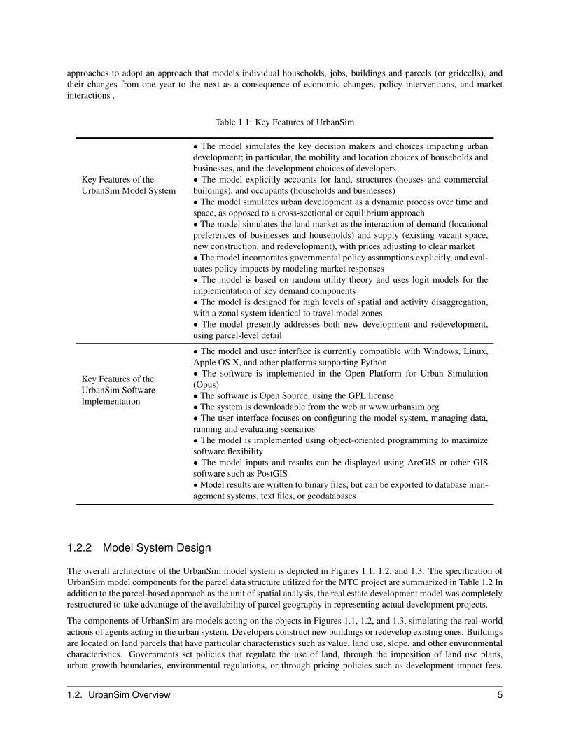
approaches to adopt an approach that models individual households, jobs, buildings and parcels (or gridcells), andtheir changes from one year to the next as a consequence of economic changes, policy interventions, and marketinteractions .
Table 1.1: Key Features of UrbanSim
Key Features of theUrbanSim Model System
• The model simulates the key decision makers and choices impacting urbandevelopment; in particular, the mobility and location choices of households andbusinesses, and the development choices of developers• The model explicitly accounts for land, structures (houses and commercialbuildings), and occupants (households and businesses)• The model simulates urban development as a dynamic process over time andspace, as opposed to a cross-sectional or equilibrium approach• The model simulates the land market as the interaction of demand (locationalpreferences of businesses and households) and supply (existing vacant space,new construction, and redevelopment), with prices adjusting to clear market• The model incorporates governmental policy assumptions explicitly, and eval-uates policy impacts by modeling market responses• The model is based on random utility theory and uses logit models for theimplementation of key demand components• The model is designed for high levels of spatial and activity disaggregation,with a zonal system identical to travel model zones• The model presently addresses both new development and redevelopment,using parcel-level detail
Key Features of theUrbanSim SoftwareImplementation
• The model and user interface is currently compatible with Windows, Linux,Apple OS X, and other platforms supporting Python• The software is implemented in the Open Platform for Urban Simulation(Opus)• The software is Open Source, using the GPL license• The system is downloadable from the web at www.urbansim.org• The user interface focuses on configuring the model system, managing data,running and evaluating scenarios• The model is implemented using object-oriented programming to maximizesoftware flexibility• The model inputs and results can be displayed using ArcGIS or other GISsoftware such as PostGIS•Model results are written to binary files, but can be exported to database man-agement systems, text files, or geodatabases
1.2.2 Model System Design
The overall architecture of the UrbanSim model system is depicted in Figures 1.1, 1.2, and 1.3. The specification ofUrbanSim model components for the parcel data structure utilized for the MTC project are summarized in Table 1.2 Inaddition to the parcel-based approach as the unit of spatial analysis, the real estate development model was completelyrestructured to take advantage of the availability of parcel geography in representing actual development projects.
The components of UrbanSim are models acting on the objects in Figures 1.1, 1.2, and 1.3, simulating the real-worldactions of agents acting in the urban system. Developers construct new buildings or redevelop existing ones. Buildingsare located on land parcels that have particular characteristics such as value, land use, slope, and other environmentalcharacteristics. Governments set policies that regulate the use of land, through the imposition of land use plans,urban growth boundaries, environmental regulations, or through pricing policies such as development impact fees.
1.2. UrbanSim Overview 5

Table 1.2: Specification of UrbanSim Model Components Using Parcel Data Structure
Model Agent Dependent Variable Functional Form
Household Location Choice Household(New or Mov-ing)
Residential BuildingWith Vacant Unit
Multinomial Logit
Employment Location Choice Establishment(New or Mov-ing)
Non-residential BuildingWith Vacant Space
Multinomial Logit
Building Location Choice Building Parcel (With VacantLand)
Multinomial Logit
Real Estate Price Parcel Price Multiple Regression
Governments also build infrastructure, including transportation infrastructure, which interacts with the distribution ofactivities to generate patterns of accessibility at different locations that in turn influence the attractiveness of these sitesfor different consumers. Households have particular characteristics that may influence their preferences and demandsfor housing of different types at different locations. Businesses also have preferences that vary by industry and size ofbusiness (number of employees) for alternative building types and locations.
The model system contains a large number of components, so in order to make the illustrations clearer, there are three‘views’ of the system. In Figure 1.1, the focus is on the flow of information related to jobs. Figure 1.2 provides ahousehold-centric view of the model system. Finally, Figure 1.3 provides a view with a focus on real estate.
6 Chapter 1. Introduction and Overview of UrbanSim
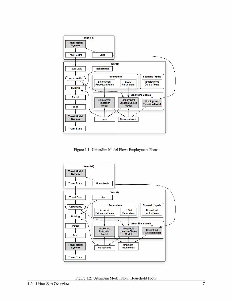
Figure 1.1: UrbanSim Model Flow: Employment Focus
Figure 1.2: UrbanSim Model Flow: Household Focus1.2. UrbanSim Overview 7
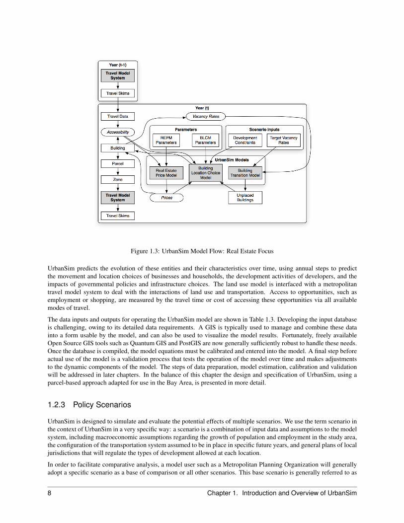
Figure 1.3: UrbanSim Model Flow: Real Estate Focus
UrbanSim predicts the evolution of these entities and their characteristics over time, using annual steps to predictthe movement and location choices of businesses and households, the development activities of developers, and theimpacts of governmental policies and infrastructure choices. The land use model is interfaced with a metropolitantravel model system to deal with the interactions of land use and transportation. Access to opportunities, such asemployment or shopping, are measured by the travel time or cost of accessing these opportunities via all availablemodes of travel.
The data inputs and outputs for operating the UrbanSim model are shown in Table 1.3. Developing the input databaseis challenging, owing to its detailed data requirements. A GIS is typically used to manage and combine these datainto a form usable by the model, and can also be used to visualize the model results. Fortunately, freely availableOpen Source GIS tools such as Quantum GIS and PostGIS are now generally sufficiently robust to handle these needs.Once the database is compiled, the model equations must be calibrated and entered into the model. A final step beforeactual use of the model is a validation process that tests the operation of the model over time and makes adjustmentsto the dynamic components of the model. The steps of data preparation, model estimation, calibration and validationwill be addressed in later chapters. In the balance of this chapter the design and specification of UrbanSim, using aparcel-based approach adapted for use in the Bay Area, is presented in more detail.
1.2.3 Policy Scenarios
UrbanSim is designed to simulate and evaluate the potential effects of multiple scenarios. We use the term scenario inthe context of UrbanSim in a very specific way: a scenario is a combination of input data and assumptions to the modelsystem, including macroeconomic assumptions regarding the growth of population and employment in the study area,the configuration of the transportation system assumed to be in place in specific future years, and general plans of localjurisdictions that will regulate the types of development allowed at each location.
In order to facilitate comparative analysis, a model user such as a Metropolitan Planning Organization will generallyadopt a specific scenario as a base of comparison or all other scenarios. This base scenario is generally referred to as
8 Chapter 1. Introduction and Overview of UrbanSim
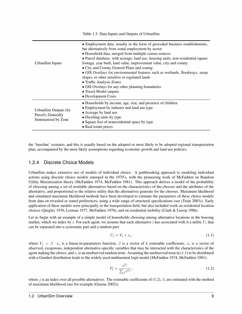
Table 1.3: Data Inputs and Outputs of UrbanSim
UrbanSim Inputs
• Employment data, usually in the form of geocoded business establishments,but alternatively from zonal employment by sector• Household data, merged from multiple census sources• Parcel database, with acreage, land use, housing units, non-residential squarefootage, year built, land value, improvement value, city and county• City and County General Plans and zoning• GIS Overlays for environmental features such as wetlands, floodways, steepslopes, or other sensitive or regulated lands• Traffic Analysis Zones• GIS Overlays for any other planning boundaries• Travel Model outputs• Development Costs
UrbanSim Outputs (byParcel), GenerallySummarized by Zone
• Households by income, age, size, and presence of children• Employment by industry and land use type• Acreage by land use• Dwelling units by type• Square feet of nonresidential space by type• Real estate prices
the ‘baseline’ scenario, and this is usually based on the adopted or most likely to be adopted regional transportationplan, accompanied by the most likely assumptions regarding economic growth and land use policies.
1.2.4 Discrete Choice Models
UrbanSim makes extensive use of models of individual choice. A pathbreaking approach to modeling individualactions using discrete choice models emerged in the 1970’s, with the pioneering work of McFadden on RandomUtility Maximization theory (McFadden 1974, McFadden 1981). This approach derives a model of the probabilityof choosing among a set of available alternatives based on the characteristics of the chooser and the attributes of thealternative, and proportional to the relative utility that the alternatives generate for the chooser. Maximum likelihoodand simulated maximum likelihood methods have been developed to estimate the parameters of these choice modelsfrom data on revealed or stated preferences, using a wide range of structural specifications (see (Train 2003)). Earlyapplication of these models were principally in the transportation field, but also included work on residential locationchoices (Quigley 1976, Lerman 1977, McFadden 1978), and on residential mobility (Clark & Lierop 1986).
Let us begin with an example of a simple model of households choosing among alternative locations in the housingmarket, which we index by i. For each agent, we assume that each alternative i has associated with it a utility Ui thatcan be separated into a systematic part and a random part:
Ui = Vi + εi, (1.1)
where Vi = β · xi is a linear-in-parameters function, β is a vector of k estimable coefficients, xi is a vector ofobserved, exogenous, independent alternative-specific variables that may be interacted with the characteristics of theagent making the choice, and εi is an unobserved random term. Assuming the unobserved term in (1.1) to be distributedwith a Gumbel distribution leads to the widely used multinomial logit model (McFadden 1974, McFadden 1981):
Pi =eVi∑j e
Vj, (1.2)
where j is an index over all possible alternatives. The estimable coefficients of (1.2), β, are estimated with the methodof maximum likelihood (see for example (Greene 2002)).
1.2. UrbanSim Overview 9
The denominator of the equation for the choice model has a particular significance as an evaluation measure. The logof this denominator is called the logsum, or composite utility, and it summarizes the utility across all the alternatives.In the context of a choice of mode between origins and destinations, for example, it would summarize the utility(disutility) of travel, considering all the modes connecting the origins and destinations. It has theoretical appeal asan evaluation measure for this reason. In fact, the logsum from the mode choice model can be used as a measure ofaccessibility.
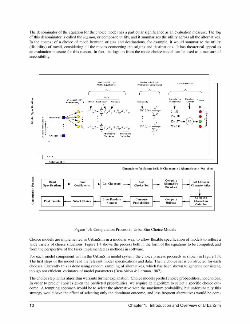
Figure 1.4: Computation Process in UrbanSim Choice Models
Choice models are implemented in UrbanSim in a modular way, to allow flexible specification of models to reflect awide variety of choice situations. Figure 1.4 shows the process both in the form of the equations to be computed, andfrom the perspective of the tasks implemented as methods in software.
For each model component within the UrbanSim model system, the choice process proceeds as shown in Figure 1.4.The first steps of the model read the relevant model specifications and data. Then a choice set is constructed for eachchooser. Currently this is done using random sampling of alternatives, which has been shown to generate consistent,though not efficient, estimates of model parameters (Ben-Akiva & Lerman 1987).
The choice step in this algorithm warrants further explanation. Choice models predict choice probabilities, not choices.In order to predict choices given the predicted probabilities, we require an algorithm to select a specific choice out-come. A tempting approach would be to select the alternative with the maximum probability, but unfortunatelty thisstrategy would have the effect of selecting only the dominant outcome, and less frequent alternatives would be com-
10 Chapter 1. Introduction and Overview of UrbanSim

pletely eliminated. In a mode choice model, for illustration, the transit mode would disappear, since the probability ofchoosing an auto mode is almost always higher than that of choosing transit. Clearly this is not a desirable or realisticoutcome. In order to address this problem, the choice algorithm used for choice models uses a sampling approach. Asillustrated in Figure 1.4, a choice outcome can be selected by sampling a random number from the uniform distributionin the range 0 to 1, and comparing this random draw to the cumulative probabilities of the alternatives. Whicheveralternative the sampled random number falls within is the alternative that is selected as the ‘chosen’ one. This algo-rithm has the property that it preserves in the distribution of choice outcomes a close approximation of the originalprobability distribution, especially as the sample size of choosers becomes larger.
1.2. UrbanSim Overview 11

CHAPTER
TWO
Bay Area UrbanSim Models
This chapter describes each of the models used in the Bay Area application of UrbanSim. The sequence of thepresentation of the models is organized approximately in the order of their execution within each simulated year, butin some cases they are grouped for clarity of exposition. All of the models operate as microsimulation models thatupdate the state of individual agents and objects: households, businesses, parcels and buildings. The state of thesimulation is updated by each model, and results are stored in annual steps from the base year of 2010 that the modeluses as its initial conditions, to the end year of 2040 for each scenario that is simulated.
2.1 Business Transition Model
2.1.1 Objective
The Business Transition Model predicts new establishments being created within or moved to the region by businesses,or the loss of establishments in the region - either through closure of a business or relocation out of the region.
Employment is classified by the user into employment sectors based on aggregations of Standard Industrial Classifi-cation (SIC) codes, or more recently, North American Industry Classification (NAICS) codes. Typically sectors aredefined based on the local economic structure. Aggregate forecasts of economic activity and sectoral employment areexogenous to UrbanSim, and are used as inputs to the model. The base year UrbanSim employment data for the MTCapplication were obtained from ABAG. The employment sectors adopted for this application are shown in Table 2.1.
The Business Transition Model integrates exogenous forecasts of aggregate employment by sector with the UrbanSimdatabase by computing the sectoral growth or decline from the preceding year, and either removing establishmentsfrom the database in sectors that are declining, or queuing establishments to be placed in the Business LocationChoice Model for sectors that experience growth. If the user supplies only total employment control totals, rather thantotals by sector, the sectoral distribution is assumed consistent with the current sectoral distribution. In cases of em-ployment loss, the probability that an establishment will be removed is assumed proportional to the spatial distributionof establishments in the sector. The establishments that are removed vacate the space they were occupying, and thisspace becomes available to the pool of vacant space for other establishments to occupy in the location component ofthe model. This procedure keeps the accounting of land, structures, and occupants up to date. New establishmentsare not immediately assigned a location. Instead, new establishments are added to the database and assigned a nulllocation, to be resolved by the Business Location Choice Model.
2.1.2 Algorithm
The model compares the total number of jobs by sector in the establishments table at the beginning of a simulationyear, to the total number of jobs by sector specified by the user in the annual employment control totals for that year.If the control total value is higher, the model adds the necessary number of establishments to the establishments tableby sampling existing establishments of the same sector and duplicating them until enough jobs have been added. If
12

the control totals indicate a declining job count for a sector then the appropriate number of establishments in the dataare selected at random and removed. The role of this model is to keep the number of jobs in the establishments data inthe simulation synchronized with aggregate expectations of employment in the region. In most current applications,control totals are separately specified for each sector and split by a proportion that is assumed to be home-basedemployment vs non-home-based employment. These two are handled by different model groups in the establishmentlocation choice model.
Table 2.1: Employment Sectors
Sector ID Sector Description
1 Professional services2 Finance, insurance, and
real estate3 Business services4 Agriculture5 Natural resources6 Arts and recreation7 Government8 Other education9 Logistics10 Eating and drinking11 Regional retail12 Social services13 Leasing14 Heavy manufacturing15 Health16 Local retail17 Transportation18 Higher education19 Utilities20 Construction21 Biotechnology22 Light manufacturing23 Information24 Hotel25 Tech manufacturing26 Personal services27 K-12 education28 Unclassified
2.1. Business Transition Model 13

2.1.3 Configuration
The configuration of the Business Transition Model in the parcel model system is summarized in the following table:
Table 2.2: Configuration of Business Transition Model
Element Setting
Agent EstablishmentsDataset EstablishmentsModel Structure Rule Based
2.1.4 Data
The following tables are used in the Business Transition Model in the parcel version of UrbanSim.
Table 2.3: Data Used by Business Transition Model
Table Name Brief Description
annual_business_control_totals Annual aggregate control totals for employment by sectorjobs jobs (synthesized from ABAG zonal employment by sector)
2.2 Household Transition Model
2.2.1 Objective
The Household Transition Model (HTM) predicts new households migrating into the region, or the loss of householdsemigrating from the region, or the net increase in households due to individuals leaving an existing household to forma new one.
The Household Transition Model accounts for changes in the distribution of households by type over time, using analgorithm analogous to that used in the Business Transition Model. In reality, these changes result from a complexset of social and demographic changes that include aging, household formation, divorce and household dissolution,mortality, birth of children, migration into and from the region, changes in household size, and changes in income,among others. The data (and theory) required to represent all of these components and their interactions adequatelyare complex, and although these behaviors have been recently implemented in UrbanSim they were not available foruse within the time constraints of this project. In this application, the Household Transition Model, like the BusinessTransition Model described above, uses external control totals of population and households by type (the latter only ifavailable) to provide a mechanism for the user to approximate the net results of these changes. Analysis by the userof local demographic trends may inform the construction of control totals with distributions of household size, age ofhead, and income. If only total population is provided in the control totals, the model assumes that the distribution ofhouseholds by type remains static.
As in the business transition case, newly created households are added to a list of movers that will be located tosubmarkets by the Household Location Choice Model. Household removals, on the other hand, are accounted for bythis model by removing those households from the housing stock, and by properly accounting for the vacancies createdby their departure. The household transition model is analogous in form to the business transition model describedabove. The primary household attributes stored on the household table in the database are shown in Table 2.4. Income
14 Chapter 2. Bay Area UrbanSim Models
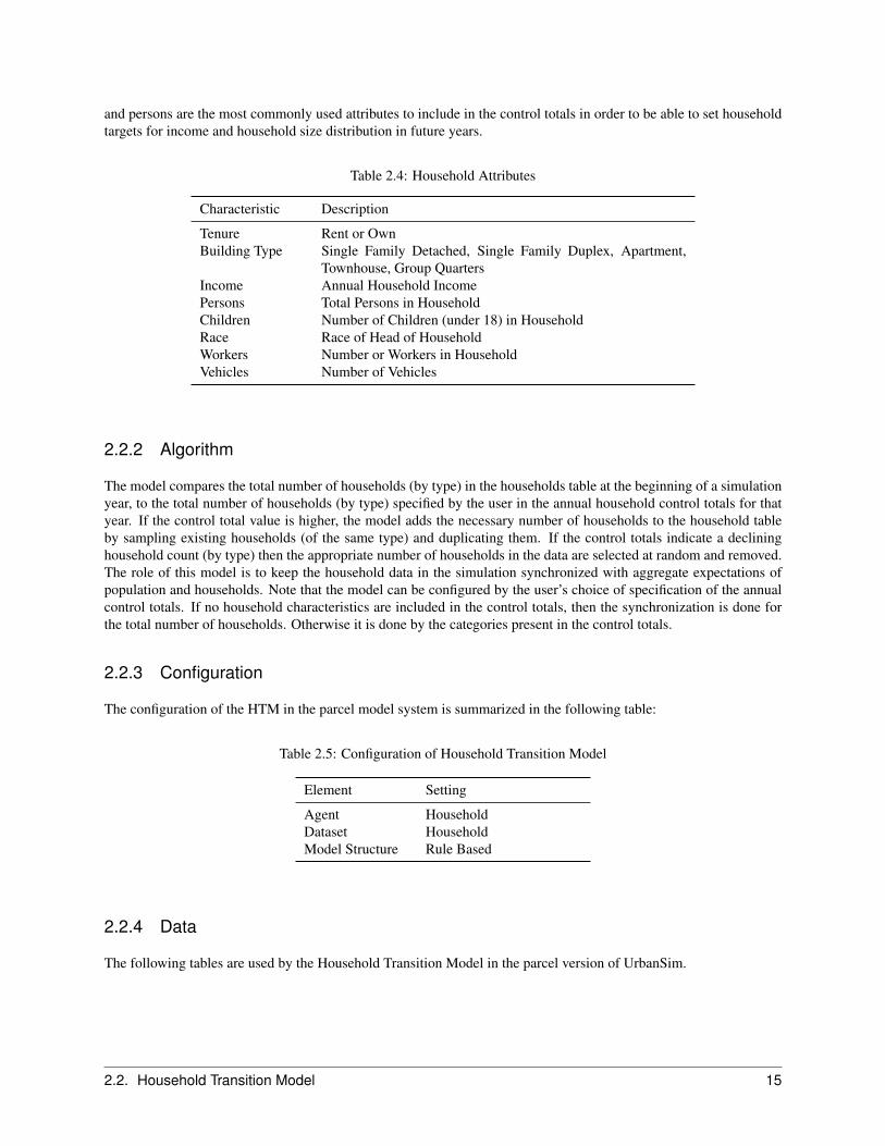
and persons are the most commonly used attributes to include in the control totals in order to be able to set householdtargets for income and household size distribution in future years.
Table 2.4: Household Attributes
Characteristic Description
Tenure Rent or OwnBuilding Type Single Family Detached, Single Family Duplex, Apartment,
Townhouse, Group QuartersIncome Annual Household IncomePersons Total Persons in HouseholdChildren Number of Children (under 18) in HouseholdRace Race of Head of HouseholdWorkers Number or Workers in HouseholdVehicles Number of Vehicles
2.2.2 Algorithm
The model compares the total number of households (by type) in the households table at the beginning of a simulationyear, to the total number of households (by type) specified by the user in the annual household control totals for thatyear. If the control total value is higher, the model adds the necessary number of households to the household tableby sampling existing households (of the same type) and duplicating them. If the control totals indicate a declininghousehold count (by type) then the appropriate number of households in the data are selected at random and removed.The role of this model is to keep the household data in the simulation synchronized with aggregate expectations ofpopulation and households. Note that the model can be configured by the user’s choice of specification of the annualcontrol totals. If no household characteristics are included in the control totals, then the synchronization is done forthe total number of households. Otherwise it is done by the categories present in the control totals.
2.2.3 Configuration
The configuration of the HTM in the parcel model system is summarized in the following table:
Table 2.5: Configuration of Household Transition Model
Element Setting
Agent HouseholdDataset HouseholdModel Structure Rule Based
2.2.4 Data
The following tables are used by the Household Transition Model in the parcel version of UrbanSim.
2.2. Household Transition Model 15
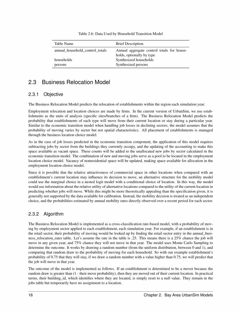
Table 2.6: Data Used by Household Transition Model
Table Name Brief Description
annual_household_control_totals Annual aggregate control totals for house-holds, optionally by type
households Synthesized householdspersons Synthesized persons
2.3 Business Relocation Model
2.3.1 Objective
The Business Relocation Model predicts the relocation of establishments within the region each simulation year.
Employment relocation and location choices are made by firms. In the current version of UrbanSim, we use estab-lishments as the units of analysis (specific sites/branches of a firm). The Business Relocation Model predicts theprobability that establishments of each type will move from their current location or stay during a particular year.Similar to the economic transition model when handling job losses in declining sectors, the model assumes that theprobability of moving varies by sector but not spatial characteristics. All placement of establishments is managedthrough the business location choice model.
As in the case of job losses predicted in the economic transition component, the application of this model requiressubtracting jobs by sector from the buildings they currently occupy, and the updating of the accounting to make thisspace available as vacant space. These counts will be added to the unallocated new jobs by sector calculated in theeconomic transition model. The combination of new and moving jobs serve as a pool to be located in the employmentlocation choice model. Vacancy of nonresidential space will be updated, making space available for allocation in theemployment location choice model.
Since it is possible that the relative attractiveness of commercial space in other locations when compared with anestablishment’s current location may influence its decision to move, an alternative structure for the mobility modelcould use the marginal choice in a nested logit model with a conditional choice of location. In this way, the modelwould use information about the relative utility of alternative locations compared to the utility of the current location inpredicting whether jobs will move. While this might be more theoretically appealing than the specification given, it isgenerally not supported by the data available for calibration. Instead, the mobility decision is treated as an independentchoice, and the probabilities estimated by annual mobility rates directly observed over a recent period for each sector.
2.3.2 Algorithm
The Business Relocation Model is implemented as a cross-classification rate-based model, with a probability of mov-ing by employment sector applied to each establishment, each simulation year. For example, if an establishment is inthe retail sector, their probability of moving would be looked up by finding the retail sector entry in the annual_busi-ness_relocation_rates table. Let’s assume the rate in the table is .25. This means there is a 25% chance the job willmove in any given year, and 75% chance they will not move in that year. The model uses Monte Carlo Sampling todetermine the outcome. It works by drawing a random number (from the uniform distribution, between 0 and 1), andcomparing that random draw to the probability of moving for each household. So with our example establishment’sprobability of 0.75 that they will stay, if we draw a random number with a value higher than 0.75, we will predict thatthe job will move in that year.
The outcome of the model is implemented as follows. If an establishment is determined to be a mover because therandom draw is greater than (1 - their move probability), then they are moved out of their current location. In practicalterms, their building_id, which identifies where they are located, is simply reset to a null value. They remain in thejobs table but temporarily have no assignment to a location.
16 Chapter 2. Bay Area UrbanSim Models
In the current application of the model in the Bay Area, the relocation rates for establishments was assumed to be zero,due to a combination of data limitations and time constraints to calibrate the model with non-zero relocation rates.This makes the location choices of businesses fixed once the establishment is assigned to a location.
2.3.3 Configuration
The configuration of the BRM is summarized in the following table:
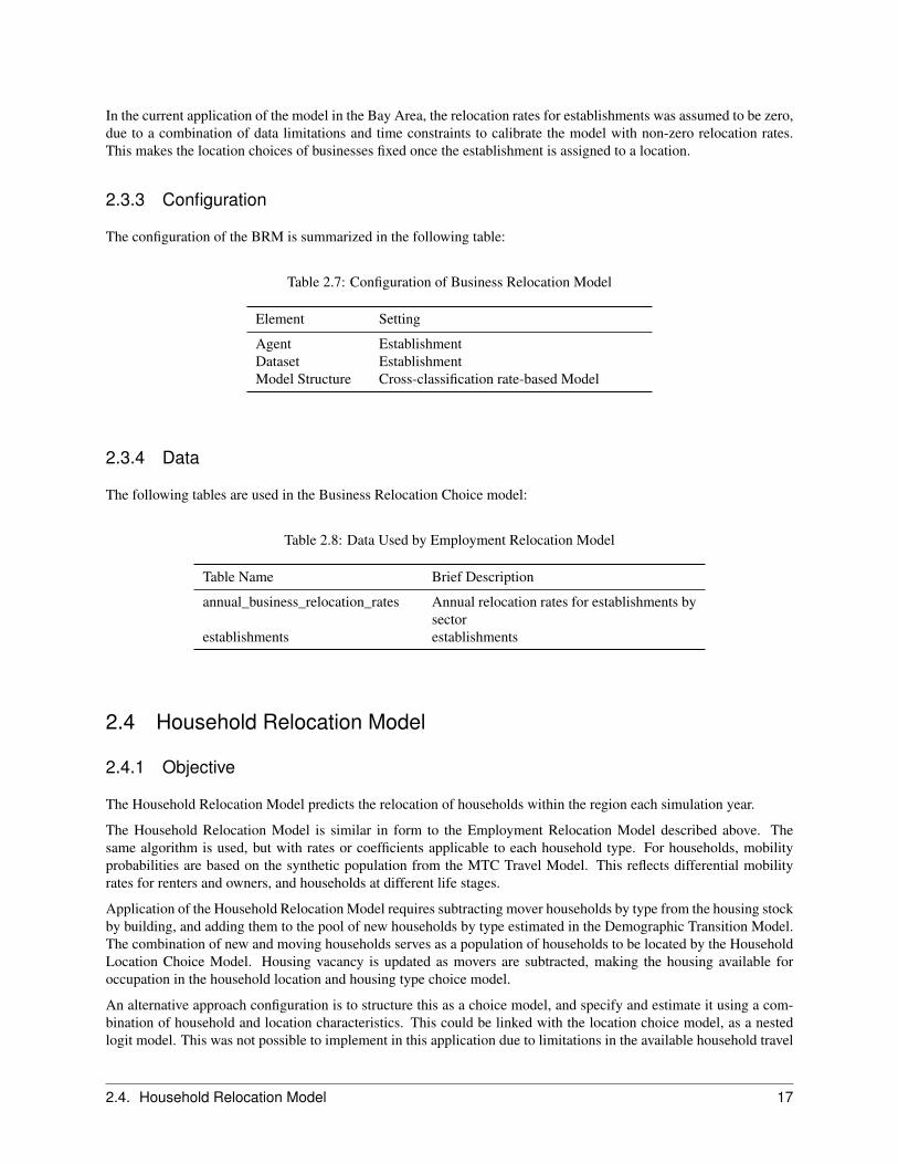
Table 2.7: Configuration of Business Relocation Model
Element Setting
Agent EstablishmentDataset EstablishmentModel Structure Cross-classification rate-based Model
2.3.4 Data
The following tables are used in the Business Relocation Choice model:
Table 2.8: Data Used by Employment Relocation Model
Table Name Brief Description
annual_business_relocation_rates Annual relocation rates for establishments bysector
establishments establishments
2.4 Household Relocation Model
2.4.1 Objective
The Household Relocation Model predicts the relocation of households within the region each simulation year.
The Household Relocation Model is similar in form to the Employment Relocation Model described above. Thesame algorithm is used, but with rates or coefficients applicable to each household type. For households, mobilityprobabilities are based on the synthetic population from the MTC Travel Model. This reflects differential mobilityrates for renters and owners, and households at different life stages.
Application of the Household Relocation Model requires subtracting mover households by type from the housing stockby building, and adding them to the pool of new households by type estimated in the Demographic Transition Model.The combination of new and moving households serves as a population of households to be located by the HouseholdLocation Choice Model. Housing vacancy is updated as movers are subtracted, making the housing available foroccupation in the household location and housing type choice model.
An alternative approach configuration is to structure this as a choice model, and specify and estimate it using a com-bination of household and location characteristics. This could be linked with the location choice model, as a nestedlogit model. This was not possible to implement in this application due to limitations in the available household travel
2.4. Household Relocation Model 17
survey, which did not contain information on relocation of households from their previous residence to their currentlocation.
2.4.2 Algorithm
The Household Relocation Model is implemented as a cross-classification rate-based model, with a probability ofmoving by age and income category applied to each household in the synthetic population, each simulation year. Forexample, if a household has head of age 31 and an income of 47,500, their probability of moving would be looked upby finding the interval within the age and income classes in the annual_household_relocation_rates table. Let’s assumethe rate in the table is .25. This means there is a 25% chance the household will move in any given year, and 75%chance they will not move in that year. The model uses Monte Carlo Sampling to determine the outcome. It works bydrawing a random number (from the uniform distribution, between 0 and 1), and comparing that random draw to theprobability of moving for each household. So with our example household’s probability of 0.75 that they will stay, ifwe draw a random number with a value higher than 0.75, we will predict that the household will move in that year.The outcome of the model is implemented as follows. If a household is determined to be a mover because the randomdraw is greater than (1 - their move probability), then they are moved out of their current location. In practical terms,their building_id, which identifies where they are located, is simply reset to a null value. They remain in the householdtable but do not have a location.
2.4.3 Configuration
The configuration of the HRM is summarized in the following table:
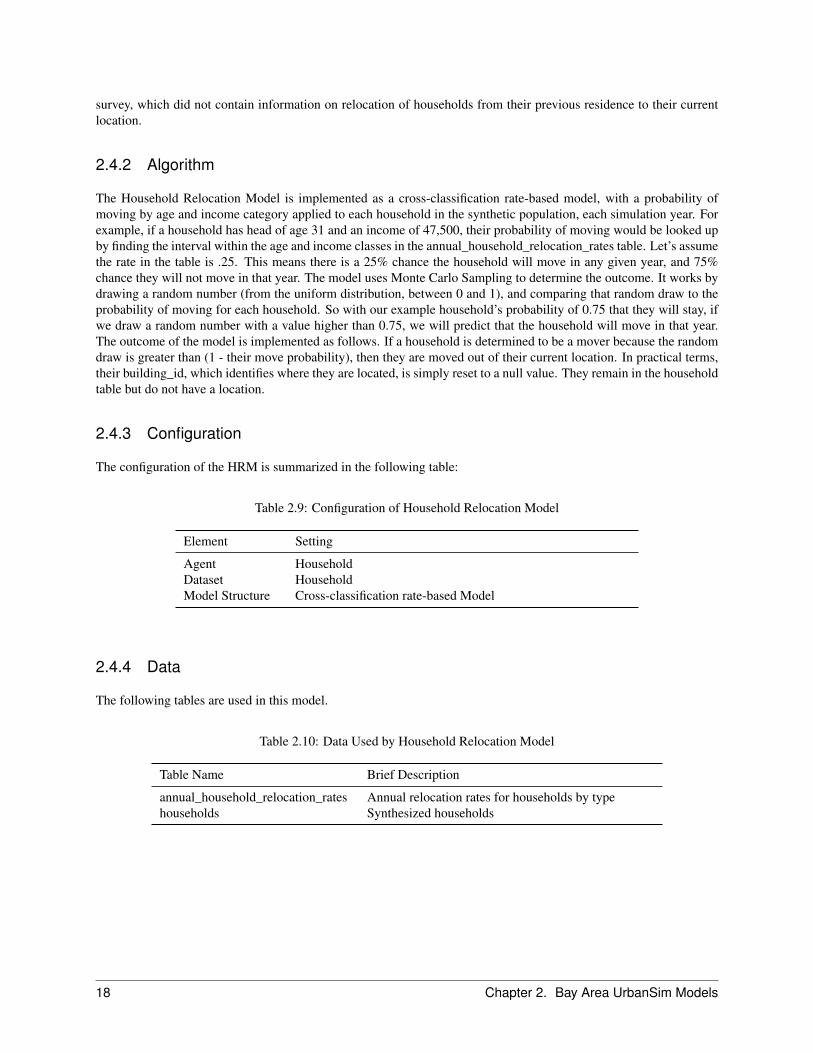
Table 2.9: Configuration of Household Relocation Model
Element Setting
Agent HouseholdDataset HouseholdModel Structure Cross-classification rate-based Model
2.4.4 Data
The following tables are used in this model.
Table 2.10: Data Used by Household Relocation Model
Table Name Brief Description
annual_household_relocation_rates Annual relocation rates for households by typehouseholds Synthesized households
18 Chapter 2. Bay Area UrbanSim Models
2.5 Household Tenure Choice Model
2.5.1 Objective
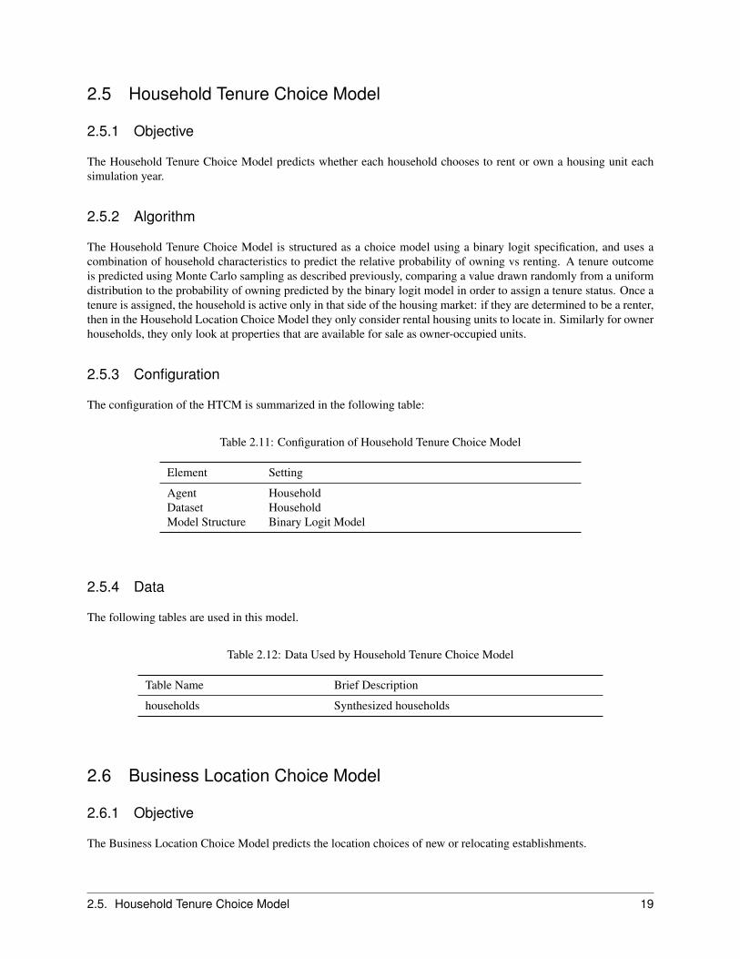
The Household Tenure Choice Model predicts whether each household chooses to rent or own a housing unit eachsimulation year.
2.5.2 Algorithm
The Household Tenure Choice Model is structured as a choice model using a binary logit specification, and uses acombination of household characteristics to predict the relative probability of owning vs renting. A tenure outcomeis predicted using Monte Carlo sampling as described previously, comparing a value drawn randomly from a uniformdistribution to the probability of owning predicted by the binary logit model in order to assign a tenure status. Once atenure is assigned, the household is active only in that side of the housing market: if they are determined to be a renter,then in the Household Location Choice Model they only consider rental housing units to locate in. Similarly for ownerhouseholds, they only look at properties that are available for sale as owner-occupied units.
2.5.3 Configuration
The configuration of the HTCM is summarized in the following table:
Table 2.11: Configuration of Household Tenure Choice Model
Element Setting
Agent HouseholdDataset HouseholdModel Structure Binary Logit Model
2.5.4 Data
The following tables are used in this model.
Table 2.12: Data Used by Household Tenure Choice Model
Table Name Brief Description
households Synthesized households
2.6 Business Location Choice Model
2.6.1 Objective
The Business Location Choice Model predicts the location choices of new or relocating establishments.
2.5. Household Tenure Choice Model 19

In this model, we predict the probability that an establishment that is either new (from the Business Transition Model),or has moved within the region (from the Business Relocation Model), will be located in a particular employmentsubmarket. Submarkets are used as the basic geographic unit of analysis in the current model implementation. Eachbusiness has an attribute of space it needs based on the employment within the establishment, and this provides a simpleaccounting framework for space utilization within submarkets. The number of locations available for an establishmentto locate within a submarket will depend mainly on the total square footage of nonresidential floorspace in buildingswithin the submarket, and on the density of the use of space (square feet per employee).
The model is specified as a multinomial logit model, with separate equations estimated for each employment sector.For both the business location and household location models, we take the stock of available space as fixed in theshort run of the intra-year period of the simulation, and assume that locators are price takers. That is, a single locatingestablishment or household does not have enough market power to influence the transaction price, and must accept thecurrent market price as given. However, the price is iteratively adjusted to account for market equilibrating tendenciesas the aggregated demand across all agents increases in some submarkets and decreases in others. This topic isdescribed in a later section on market price equilibration.
The variables included in the business location choice model are drawn from the literature in urban economics. Weexpect that accessibility to population, particularly high-income population, increases bids for retail and service busi-nesses. We also expect that two forms of agglomeration economies influence location choices: localization economiesand inter-industry linkages.
Localization economies represent positive externalities associated with locations that have other firms in the sameindustry nearby. The basis for the attraction may be some combination of a shared skilled labor pool, comparisonshopping in the case of retail, co-location at a site with highly desirable characteristics, or other factors that causethe costs of production to decline as greater concentration of businesses in the industry occurs. The classic exampleof localization economies is Silicon Valley. Inter-industry linkages refer to agglomeration economies associated withlocation at a site that has greater access to businesses in strategically related, but different, industries. Examples includemanufacturers locating near concentrations of suppliers in different industries, or distribution companies locatingwhere they can readily service retail outlets.
One complication in measuring localization economies and inter-industry linkages is determining the relevant distancefor agglomeration economies to influence location choices. At one level, agglomeration economies are likely to affectbusiness location choices between states, or between metropolitan areas within a state. Within a single metropolitanarea, we are concerned more with agglomeration economies at a scale relevant to the formation of employment cen-ters. The influence of proximity to related employment may be measured using two scales: a regional scale effectusing zone-to-zone accessibilities from the travel model, or highly localized accessibilities using queries of the areaimmediately around the given parcel. Most of the spatial queries used in the model are of the latter type, because theregional accessibility variables tend to be very highly correlated, and because agglomerations are expected to be verylocalized.
Age of buildings is included in the model to estimate the influence of age depreciation of commercial buildings,with the expectation that businesses prefer newer buildings and discount their bids for older ones. This reflects thedeterioration of older buildings, changing architecture, and preferences, as is the case in residential housing. Thereis the possibility that significant renovation will make the actual year built less relevant, and we would expect thatthis would dampen the coefficient for age depreciation. We do not at this point attempt to model maintenance andrenovation investments and the quality of buildings.
Density, the inverse of lot size, is included in the location choice model. We expect businesses, like households, toreveal different preferences for land based on their production functions and the role of amenities such as green spaceand parking area. As manufacturing production continues to shift to more horizontal, land-intensive technology, weexpect the discounting for density to be relatively high. Retail, with its concentration in shopping strips and malls, stillrequires substantial surface land for parking, and is likely to discount bids less for density. We expect service firmsto discount for density the least, since in the traditional urban economics models of bid-rent, service firms generallyoutbid other firms for sites with higher accessibility, land cost, and density.
We might expect that certain sectors, particularly retail, show some preference for locations near a major highway,and are willing to bid higher for those locations. Distance to a highway is measured in meters, using grid spatialqueries. We also test for the residual influence of the classic monocentric model, measured by travel time to the CBD,
20 Chapter 2. Bay Area UrbanSim Models
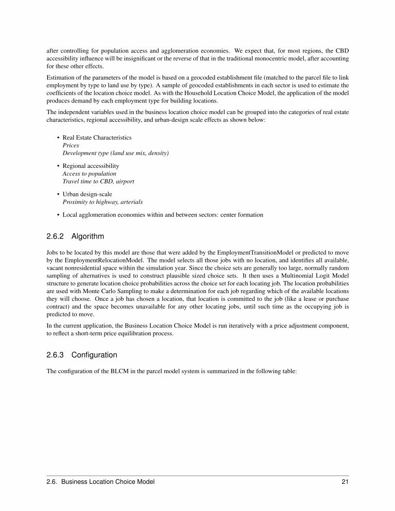
after controlling for population access and agglomeration economies. We expect that, for most regions, the CBDaccessibility influence will be insignificant or the reverse of that in the traditional monocentric model, after accountingfor these other effects.
Estimation of the parameters of the model is based on a geocoded establishment file (matched to the parcel file to linkemployment by type to land use by type). A sample of geocoded establishments in each sector is used to estimate thecoefficients of the location choice model. As with the Household Location Choice Model, the application of the modelproduces demand by each employment type for building locations.
The independent variables used in the business location choice model can be grouped into the categories of real estatecharacteristics, regional accessibility, and urban-design scale effects as shown below:
• Real Estate CharacteristicsPricesDevelopment type (land use mix, density)
• Regional accessibilityAccess to populationTravel time to CBD, airport
• Urban design-scaleProximity to highway, arterials
• Local agglomeration economies within and between sectors: center formation
2.6.2 Algorithm
Jobs to be located by this model are those that were added by the EmploymentTransitionModel or predicted to moveby the EmploymentRelocationModel. The model selects all those jobs with no location, and identifies all available,vacant nonresidential space within the simulation year. Since the choice sets are generally too large, normally randomsampling of alternatives is used to construct plausible sized choice sets. It then uses a Multinomial Logit Modelstructure to generate location choice probabilities across the choice set for each locating job. The location probabilitiesare used with Monte Carlo Sampling to make a determination for each job regarding which of the available locationsthey will choose. Once a job has chosen a location, that location is committed to the job (like a lease or purchasecontract) and the space becomes unavailable for any other locating jobs, until such time as the occupying job ispredicted to move.
In the current application, the Business Location Choice Model is run iteratively with a price adjustment component,to reflect a short-term price equilibration process.
2.6.3 Configuration
The configuration of the BLCM in the parcel model system is summarized in the following table:
2.6. Business Location Choice Model 21

Table 2.13: Configuration of Bmployment Location Choice Model
Element Setting
Agent EstablishmentLocation Set Employment submarkets - which are defined by jurisdiction,
building type, and transit proximity.Dependent Variable Location of each establishment: employment_submarket_idModel Type Multinomial Logit ModelEstimation Method Maximum LikelihoodSubmodels Sector - separate models are specified for groups of jobs by em-
ployment sectorIndependent Variables Attributes of submarkets: Price, density, accessibility, composi-
tion of households and employment
2.6.4 Data
The following tables are used by the Business Location Choice Model:
Table 2.14: Data Used by Business Location Choice Model
Table Name Brief Description
establishment Establishments table with an inventory of employmentemployment_sectors Employment sectors, defined using NAICS or SIC
classifications of industrybuildings Buildings from which available non-residential sqft
are evaluated for locationzones Zones are used to compute density, social composition,
and accessibility variablestravel_data Skims from the travel model are used to compute ac-
cessibility variables
2.7 Household Location Choice Model
2.7.1 Objective
The Household Location Choice Model (HLCM) predicts the location choices of new or relocating renter and ownerhouseholds.
In this model, as in the employment location model, we predict the probability that a household that is either new (fromthe transition component), or has decided to move within the region (from the household relocation model) and hasdetermined whether to rent or own a unit (from the household tenure choice model), will choose a particular locationdefined by a residential submarket. As before, the form of the model is specified as multinomial logit, with randomsampling of alternatives from the universe of submarkets with vacant housing.
For both the household location and business location models, we take the stock of available space as fixed in theshort run of the intra-year period of the simulation, and assume that locators are price takers. That is, a single locatinghousehold does not have enough market power to influence the transaction price (or rent), and must accept the current
22 Chapter 2. Bay Area UrbanSim Models

market price as given. However, the price (or rent) is iteratively adjusted to account for market equilibrating tenden-cies as the aggregated demand across all agents increases in some submarkets and decreases in others. This topic isdescribed in a later section on market price equilibration.
The model architecture allows location choice models to be estimated for households stratified by income level, thepresence or absence of children, and other life cycle characteristics. Alternatively, these effects can be included in asingle model estimation through interactions of the household characteristics with the characteristics of the alternativelocations. The current implementation is based on the latter but is general enough to accommodate stratified estimation,for example by household income.
For the Bay Area application of the model, households are stratified by 4 income categories cross-classified with house-hold size of 1, 2, 3 or more. Income and household size provide a strong basis for differentiating among consumerswith substantially different preferences and trade-offs in location choices.
We further differentiate households by their tenure choice, given the importance of this distinction for understandingthe impacts of housing prices and rents on location choices. Predictions of tenure for each household are made by theHousehold Tenure Choice Model, discussed in Section 2.5.
The variables used in the model are drawn from the literature in urban economics, urban geography, and urban sociol-ogy. An initial feature of the model specification is the incorporation of the classical urban economic trade-off betweentransportation and land cost. This has been generalized to account not only for travel time to the classical monocentriccenter, the CBD, but also to more generalized access to employment opportunities and to shopping. These accessi-bilities to work and shopping are measured by weighting the opportunities at each destination zone with a compositeutility of travel across all modes to the destination, based on the logsum from the mode choice travel model.
These measures of accessibility should negate the traditional pull of the CBD, and, for some population segments,potentially reverse it. In addition to these accessibility variables, we include in the model a net building density, tomeasure the input-substitution effect of land and capital. To the extent that land near high accessibility locations is bidup in price, we should expect that builders will substitute capital for land and build at higher densities. Consumers forwhom land is a more important amenity will choose larger lot housing with less accessibility, and the converse shouldhold for households that value accessibility more than land, such as higher income childless households.
The age of housing is considered for two reasons. First, we should expect that housing depreciates with age, sincethe expected life of a building is finite, and a consistent stream of maintenance investments are required to slow thedeterioration of the structure once it is built. Second, due to changing architectural styles, amenities, and tastes, weshould expect that the wealthiest households prefer newer housing, all else being equal. The exception to this patternis likely to be older, architecturally interesting, high quality housing in historically wealthy neighborhoods. Thepreference for these alternatives are accommodated through a combination of nonlinear or dummy variable treatmentfor this type of housing and neighborhood.
A related hypothesis from urban economics is that, since housing is considered a normal good, it has a positive incomeelasticity of demand. This implies that as incomes rise, households will spend a portion of the gains in income topurchase housing that is more expensive, and that provides more amenities (structural and neighborhood) than theirprior dwelling. A similar hypothesis is articulated in urban sociology in which upward social mobility is associatedwith spatial proximity to higher status households. Both of these hypotheses predict that households of any givenincome level prefer, all else being equal, to locate in neighborhoods that have higher average incomes. (UrbanSimdoes not attempt to operationalize the concepts of social status or social assimilation, but does consider income in thelocation choice.)
The age hypothesis and the two income-related hypotheses are consistent with the housing filtering model, whichexplains the dynamic of new housing construction for wealthy households that sets in motion a chain of vacancies.The vacancy chain causes households to move into higher status neighborhoods than the ones they leave, and housingunits to be successively occupied by lower and lower status occupants. At the end of the vacancy chain, in the leastdesirable housing stock and the least desirable neighborhoods, there can be insufficient demand to sustain the housingstock and vacancies go unsatisfied, leading ultimately to housing abandonment. We include in the model an agedepreciation variable, along with a neighborhood income composition set of variables, to collectively test the housingfiltering and related hypotheses.
One of the features that households prefer is a compatible land use mix within the neighborhood. It is likely that
2.7. Household Location Choice Model 23

residential land use, as a proxy for land uses that are compatible with residential use, positively influences housingbids. On the other hand, industrial land use, as a proxy for less desirable land use characteristics, would lower bids.
The model parameters are estimated using a random sample of alternative locations, which has been shown to provideconsistent estimates of the coefficients. In application for forecasting, each locating household is modeled individually,and a sample of alternative cell locations is generated in proportion to the available (vacant) housing. Monte carlosimulation is used to select the specific alternative to be assigned to the household, and vacant and occupied housingunits are updated in the cell.
The independent variables can be organized into the three categories of housing characteristics, regional accessibility,and urban-design scale effects as shown below.
• Housing CharacteristicsPrices (interacted with income)Development types (density, land use mix) Housing age
• Regional accessibilityJob accessibility by auto-ownership groupTravel time to CBD and airport
• Urban design-scale (local accessibility)Neighborhood land use mix and densityNeighborhood Employment
2.7.2 Algorithm
Households to be located by this model are those that were added by the HouseholdTransitionModel or predicted tomove by the HouseholdRelocationModel. The model selects all those households of a specified tenure status (renter orowner) that need to find a housing unit, and identifies all available, vacant housing units within the simulation year thatare of the appropriate tenure. Since the choice sets are generally too large, normally random sampling of alternativesis used to construct plausible sized choice sets. It then uses a Multinomial Logit Model structure to generate locationchoice probabilities across the choice set for each household. The location probabilities are used with Monte CarloSampling to make a determination for each household regarding which of the available locations they will choose.Once a household has chosen a location, that location is committed to the household (like a rental contract or closingon a purchase of a house) and the residential unit becomes unavailable for any other households, until such time as theoccupying household is predicted to move.
24 Chapter 2. Bay Area UrbanSim Models

2.7.3 Configuration
The configuration of the Household Location Choice Model is summarized in the following table:
Table 2.15: Configuration of Household Location Choice Model
Element Setting
Agent JobLocation Set Residential submarkets - which are defined by building type,
school district, tenure, and transit proximityDependent Variable Location of each household: submarket_idModel Type Multinomial Logit ModelEstimation Method Maximum LikelihoodSubmodels Separate models can be specified for groups of householdsIndependent Variables Attributes of households interacted with attributes of submarkets
2.7.4 Data
The following tables are used by the Household Location Choice Model.
Table 2.16: Data Used by Household Location Choice Model
Table Name Brief Description
households Synthetic households tablebuildings Buildings from which available residential units are
evaluated for locationzones Zones are used to compute density, social composition,
and accessibility variablestravel_data Skims from the travel model are used to compute ac-
cessibility variables
2.8 Real Estate Price Model
2.8.1 Objective
The Real Estate Price Model (REPM) predicts the price per unit of each building. For residential units, the sale priceis estimated for owner units, and the rent is estimated for rental units.
UrbanSim uses real estate prices as the indicator of the match between demand and supply of land at different locationsand with different land use types, and of the relative market valuations for attributes of housing, nonresidential space,and location. This role is important to the rationing of land and buildings to consumers based on preferences andability to pay, as a reflection of the operation of actual real estate markets. Since prices enter the location choice utilityfunctions for jobs and households, an adjustment in prices will alter location preferences. All else being equal, this willin turn cause higher price alternatives to become more likely to be chosen by occupants who have lower price elasticityof demand. Similarly, any adjustment in land prices alters the preferences of developers to build new construction bytype of space, and the density of the construction.
2.8. Real Estate Price Model 25

We make the following assumptions:
1. Households, businesses, and developers are all price-takers individually, and market adjustments are made bythe market in response to aggregate demand and supply relationships.
2. Location preferences and demand-supply imbalances are capitalized into land values. Building value reflectsbuilding replacement costs only, and can include variations in development costs due to terrain, environmentalconstraints or development policy.
Following on these assumptions and the best available theory regarding real estate price formation, we begin with areduced-form hedonic regression model to establish the initial price and rent estimates based on stuctural and loca-tional attributes, and combine this with a second step that incorporates short-term (within a year) market equilbratingtendencies.
2.8.2 Hedonic Price Regression
Real estate prices are modeled using a hedonic regression of the log-transformed property value per square foot onattributes of the parcel and its environment, including land use mix, density of development, proximity of highwaysand other infrastructure, land use plan or zoning constraints, and neighborhood effects. The hedonic regression maybe estimated from sales transactions if there are sufficient transactions on all property types, and if there is sufficientinformation on the lot and its location. An alternative is to use tax assessor records on land values, which are partof the database typically assembled to implement the model. Although assessor records may contain biases in theirassessment, they do provide virtually complete coverage of the land (with notable exceptions and gaps for exempt orpublicly owned property).
The hedonic regression equation encapsulates interactions between market demand and supply, revealing an envelopeof implicit valuations for location and structural characteristics (DiPasquale & Wheaton 1996). Prices are updated byUrbanSim annually, after all construction and market activity is completed. These end of year prices are then used asthe values of reference for market activities in the subsequent year.
The independent variables influencing land prices can be organized into site characteristics, regional accessibility, andurban-design scale effects, as shown below:
• Site characteristicsDevelopment typeLand use planEnvironmental constraints
• Regional accessibilityAccess to population and employment
• Urban design-scaleLand use mix and densityProximity to highway and arterials
Algorithm
The Real Estate Price Model uses a hedonic regression structure, which is a multiple regression, estimated usingOrdinary Least Squares (OLS), normally with the price specified as a log of price.
Configuration
The configuration of the REPM in the parcel model system is summarized in the following table:
26 Chapter 2. Bay Area UrbanSim Models

Table 2.17: Configuration of Real Estate Price Model
Element Setting
Dataset BuildingsDependent Variable Log of Price Per Unit (per housing unit for residential, per square
foot for non-residential buildings)Model Type RegressionSubmodels Separate models are specified for each type of buildingIndependent Variables Constant, and attributes of building: density, accessibility, zonal
composition of households and employment
Data
These tables are used by the Real Estate Price Model:
Table 2.18: Data Used by Real Estate Price Model
Table Name Brief Description
buildings Individual buildings located on parcels (can be many per parcel)residential_units Individual residential units located within a buildingzones Zones used in the travel model, for accessibility and density variablestravel_data Zone-to-zone skims from the travel model, for accessibility variableshouseholds Household data, for socioeconomic and density variablesjobs Employment data, for accessibility and density variables
2.8.3 Market Price Equilibration
In order to reflect the role of equilibrating tendencies in the market, we have introduced to the Bay Are model ap-plication a dampened price equilibration algorithm first described in (Wang & Waddell 2013). The market priceequilibration algorithm we use reflects the impact of aggregated individual demands at each submarket on prices, andthe resulting effects of the altered prices on individual choice probabilities, inducing a circular causality which requiresa fixed point algorithm in order to solve for the market clearing prices. Below is the algorithm for computing the fullmarket price clearing array of prices and demands for each submarket, which we then dampen to reflect partial ad-justment towards equilibrium, in recognition of real-world frictional factors that prevent full equilibration within onetime period. The dampening factor used for this model application was calibrated to 0.2, meaning that prices adjustone-fifth of the way towards full equilibrium within one year.
We assume a random utility maximization framework as the basis of the residence choices. Let the probability thathousehold (business) n chooses location i from the set C of available residence (business) locations be given by thefollowing multinomial logit form:
Pni = Pr(Uni ≥ Unj ,∀j ∈ C) =eVni∑
j∈C eVnj
(2.1)
We further assume price in Vni will be adjusted so that the discrepancy between the supply and aggregated demand bysubmarket is minimized:
arg minprice
∑i(Si −Di)
2, subject to price ∈ (Lower Bound, Upper Bound), (2.2)
2.8. Real Estate Price Model 27
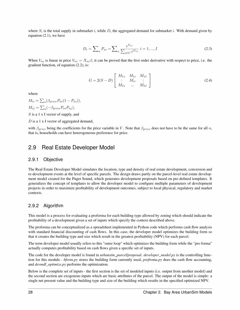
where Si is the total supply in submarket i, while Di the aggregated demand for submarket i. With demand given byequation (2.1), we have
Di =∑
nPni =
∑n
eVni∑j∈C e
Vnji = 1, ..., I (2.3)
When Vni is linear in price Vni = Xniβ, it can be proved that the first order derivative with respect to price, i.e. thegradient function, of equation (2.2), is:
G = 2(S −D)
M11 M1i M1I
: Mii :MI1 ... MII
(2.4)
where
Mii =∑
n(βpricePni(1− Pni)),
Mij =∑
n(−βpricePniPnj),
S is a 1 x I vector of supply, and
D is a 1 x I vector of aggregated demand,
with βprice being the coefficients for the price variable in V . Note that βprice does not have to be the same for all n,that is, households can have heterogeneous preference for price.
2.9 Real Estate Developer Model
2.9.1 Objective
The Real Estate Developer Model simulates the location, type and density of real estate development, conversion andre-development events at the level of specific parcels. The design draws partly on the parcel-level real estate develop-ment model created for the Puget Sound, which generates development proposals based on pre-defined templates. Itgeneralizes the concept of templates to allow the developer model to configure multiple parameters of developmentprojects in order to maximize profitability of development outcomes, subject to local physical, regulatory and marketcontexts.
2.9.2 Algorithm
This model is a process for evaluating a proforma for each building type allowed by zoning which should indicate theprofitability of a development given a set of inputs which specify the context described above.
The proforma can be conceptualized as a spreadsheet implemented in Python code which performs cash flow analysiswith standard financial discounting of cash flows. In this case, the developer model optimizes the building form sothat it creates the building type and size which result in the greatest profitability (NPV) for each parcel.
The term developer model usually refers to this "outer loop" which optimizes the building form while the "pro forma"actually computes profitability based on cash flows given a specific set of inputs.
The code for the developer model is found in urbansim_parcel/proposal. developer_model.py is the controlling func-tion for this module - bform.py stores the building form currently used, profroma.py does the cash flow accounting,and devmdl_optimize.py performs the optimization.
Below is the complete set of inputs - the first section is the set of modeled inputs (i.e. output from another model) andthe second section are exogenous inputs which are basic attributes of the parcel. The output of the model is simple: asingle net present value and the building type and size of the building which results in the specified optimized NPV.
28 Chapter 2. Bay Area UrbanSim Models

For this application, the developer model runs each simulated year on all empty parcels, on all parcels within a PDA,on parcels within 800m of Caltrain and BART, and a sampled portion of the other parcels to capture redevelopermentof parcels.
For redevelopment, demolition cost is computed through one of the following: the value of residential owner housing,a simple multiplier for residential rental housing, the price estimated for nonresidential sqft, and a land price based onthe value of nearby building prices.
Policies enter the developer model by the zoning (primarily by allowed FAR and building types), and also with a parcelsubsidy/fee that is specified for each parcel.
2.9.3 Data
Table 2.19: Data Used by Real Estate Developer Model
Variable Name Brief Description
PRICESsingle family Price estimate for single-family housingmulti family Price estimate for multi-family housingrent single family Rent estimate for single-family housingrent multi family Rent estimate for multi-family housingoffice Rent estimate for the office building typeretail Rent estimate for the retail building typeindustrial Rent estimate for the industrial building typeABSORPTIONsales absorption The absorption rate for sales units by building typesales vacancy The vacancy rate for sales units by building typerent absorption The absorption rate for rental units by building typerent vacancy rates The vacancy rate for rental units by building typeSIZESaverage lot size Typical lot size in the zone for this parcelsf unit size Typical single-family unit size in the zone for this parcelmf unit size Typical multi-family unit size in the zone for this parcelZONINGbuilding types Allowable building types for this parcelFAR Floor area ratio allowed for this parcelheight Height limits for this parcelmax_dua Max dwelling units for this parcelPOLICIESRegional devel-opment fee
Whether to apply indirect source rule. Regional development fees areuser-specified
unit subsidy User-specified per-unit subsidiesper sqft subsidy User-specified per-unit subsidies for non-residential square feet
2.9. Real Estate Developer Model 29

2.10 Government and Schools Allocation
2.10.1 Objective
Government and public education jobs are not typically a part of the market-based economy, and the allocation ofthese jobs does not occur in the same way as other market-based jobs. Since these jobs are more closely tied to thegeographic distribution of the population and the locations of existing government and education jobs, a differentmodel was developed for allocating jobs in the government and public education sectors. The basis of the governmentand education jobs allocation was that local government jobs and local schools jobs would grow along with the localpopulation. There would be potential for new locations for schools and local government facilities within the commu-nity, but with more of the jobs expected at existing locations. For county, state, federal and higher education jobs, onthe other hand, would grow with the county and regional population, and only in locations of existing government andeducation jobs and at roughly the same proportions.
2.10.2 Algorithm
To allocate future government and education jobs, coefficients were developed for each TAZ to represent rates of jobsper population. The coefficients were developed in a multi-step process.
Three classes of jobs were identified in the government and public education sectors:
1. Jobs based on the local city-level population; these jobs include jobs with local government agencies and jobswith local public primary and secondary schools.
2. Jobs based on the county-level population; these jobs include county government and special district jobs.
3. Jobs based on the regional-level population; these include state and federal government jobs, and jobs at publicinstitutions of higher education.
Each of the government establishments in the NETS dataset was then coded as local, county, or regional. Similarly,each of the public education establishments were coded as local or regional.
For local jobs, using the 2010 Census population totals by city and the NETS job distribution, rates of government andeducation employees were calculated for each city by city jobs by city 2010 population. The coefficient for each TAZis calculated by the following equation:
c = Jobs2010 + PopGrowth ∗RateCity ∗ Pop2040 (2.5)
where
c is the TAZ coefficient for local government jobs or local education jobs. For the local education jobs, c cannot exceedthe twice the citywide jobs per population rate; for the local government jobs coefficient, c cannot exceed 5 times thecity wide jobs per population rate.
Jobs2010 is the total local jobs in the TAZ - local government or education, depending on the coefficient.
PopGrowth is the estimated population growth in the TAZ.
RateCity is 2010 city jobs divided by the 2010 city population.
Pop2040 = the estimated 2040 population in the TAZ.
The calculation of the coefficients for the county - and regional-based jobs is more straight forward. For countyjobs, the coefficient was calculated by dividing the total county jobs in the TAZ by the county population. Separatecoefficients were developed for state, federal and higher education jobs, but each was calculated in the same manner.The coefficient for each TAZ equals the total 2010 jobs divided by total 2010 regional population.
30 Chapter 2. Bay Area UrbanSim Models

The result is a set of 6 coefficients for each TAZ: for local education jobs, local government jobs, county governmentjobs, state government jobs, federal government jobs (includes other regionally-based jobs), and for higher educationjobs. Each coefficient is applied to the total TAZ population to derive the TAZ-level government and education jobsby type. The final step is to rebalance the totals proportionally to meet regional control totals.
2.11 The Role of Accessibility
Accessibility is a very important influence in urban space, and it similarly plays an important role in UrbanSim.Almost all models in UrbanSim consider the effects of accessibility. But unlike the monocentric or spatial interactionmodels, in which the choice of workplace is exogenous and residential locations are chosen principally on the basis ofcommute to the city center or to a predetermined workplace, we deal with accessibility in a more general framework.Accessibility is considered a normal good, like other positive attributes of housing, which consumers place a positiveeconomic value on. We therefore expect that consumers value access to workplaces and shopping opportunities,among the many other attributes they consider in their housing preferences. However, not all households respondto accessibility in the same way. Retired persons would be less influenced by accessibility to job opportunities thanwould working age households, for instance.
We operationalize the concept of accessibility for a given location as the distribution of opportunities weighted bythe travel impedance, or alternatively the utility of travel to those destinations. A number of alternative accessibilitymeasures have been developed in UrbanSim.
The accessibility model reads the auto and transit accessibility measures from the travel model, as well as the land usedistribution for a given year, and creates accessibility indices for use in the household and business location choicemodels. The general framework is to summarize the accessibility from each zone to various activities for whichaccessibility is considered important in household or business location choice.
Since UrbanSim operates annually, but travel model updates are likely to be executed for two to three of the yearswithin the forecasting horizon, travel utilities remain constant from one travel model run until they are replaced by thenext travel model result.
2.12 User-Specified Events
Given our current understanding, no model will be able to simulate accurately the timing, location and nature of majorevents such as a major corporate relocation into or out of a metropolitan area, or a major development project such as aregional shopping mall. In addition, major policy events, such as a change in the land use plan or in an Urban GrowthBoundary, are outside the range of predictions of our simulation. (At least in its current form, UrbanSim is intendedas a tool to aid planning and civic deliberation, not as a tool to model the behavior of voters or governments. We wantit to be used to say “if you adopt the following policy, here are the likely consequences," but not to say “UrbanSimpredicts that in 5 years the county will adopt the following policy.")
However, planners and decision-makers often have information about precisely these kinds of major events, and thereis a need to integrate such information into the use of the model system. It is useful, for example, to explore thepotential effects of a planned corporate relocation by introducing user-specified events to reflect the construction ofthe corporate building, and the relocation into the region (and to the specific site) of a substantial number of jobs,and examine the cumulative or secondary effects of the relocation on further residential and employment location andreal estate development choices. Inability to represent such events, in the presence of knowledge about developmentsthat may be ‘in the pipeline,’ amounts to less than full use of the available information about the future, and couldundermine the validity and credibility of the planning process. For these reasons, support for three kinds of events hasbeen incorporated into the system: development events, employment events, and policy events.
2.11. The Role of Accessibility 31
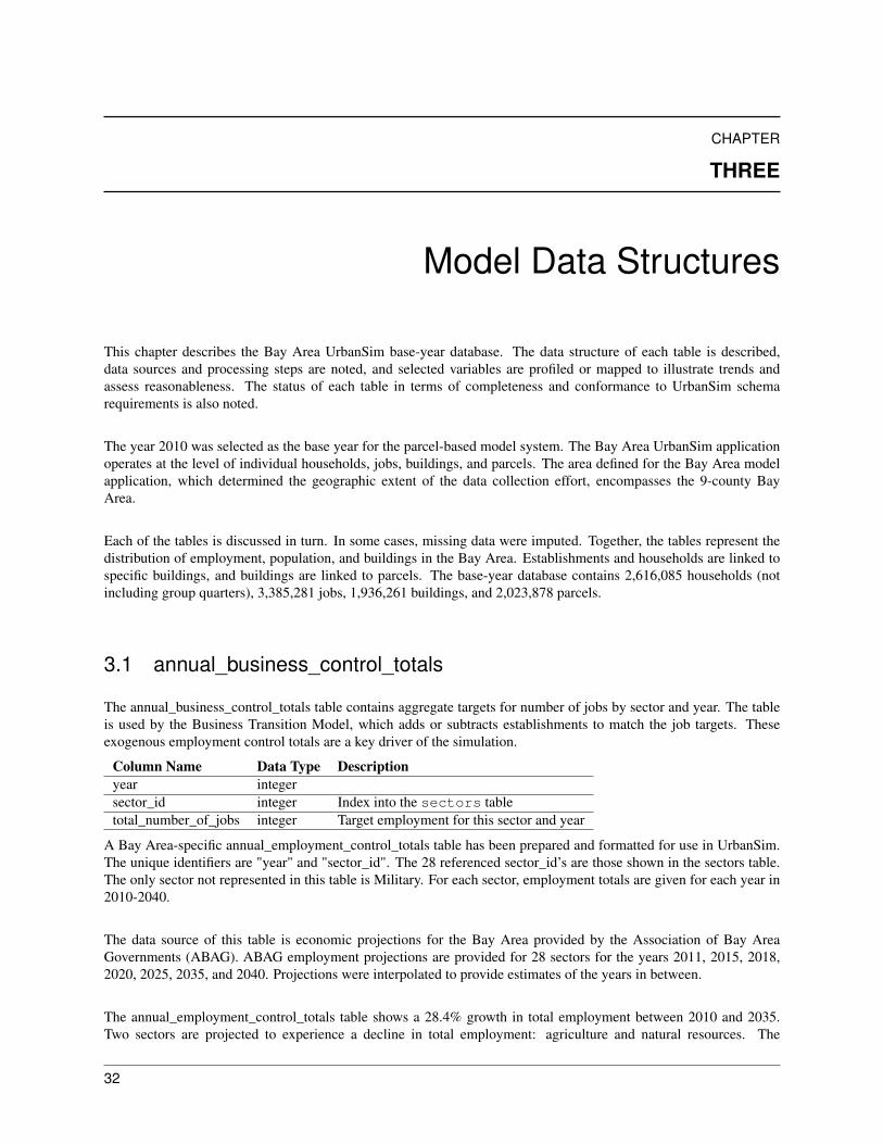
CHAPTER
THREE
Model Data Structures
This chapter describes the Bay Area UrbanSim base-year database. The data structure of each table is described,data sources and processing steps are noted, and selected variables are profiled or mapped to illustrate trends andassess reasonableness. The status of each table in terms of completeness and conformance to UrbanSim schemarequirements is also noted.
The year 2010 was selected as the base year for the parcel-based model system. The Bay Area UrbanSim applicationoperates at the level of individual households, jobs, buildings, and parcels. The area defined for the Bay Area modelapplication, which determined the geographic extent of the data collection effort, encompasses the 9-county BayArea.
Each of the tables is discussed in turn. In some cases, missing data were imputed. Together, the tables represent thedistribution of employment, population, and buildings in the Bay Area. Establishments and households are linked tospecific buildings, and buildings are linked to parcels. The base-year database contains 2,616,085 households (notincluding group quarters), 3,385,281 jobs, 1,936,261 buildings, and 2,023,878 parcels.
3.1 annual_business_control_totals
The annual_business_control_totals table contains aggregate targets for number of jobs by sector and year. The tableis used by the Business Transition Model, which adds or subtracts establishments to match the job targets. Theseexogenous employment control totals are a key driver of the simulation.
Column Name Data Type Descriptionyear integersector_id integer Index into the sectors tabletotal_number_of_jobs integer Target employment for this sector and year
A Bay Area-specific annual_employment_control_totals table has been prepared and formatted for use in UrbanSim.The unique identifiers are "year" and "sector_id". The 28 referenced sector_id’s are those shown in the sectors table.The only sector not represented in this table is Military. For each sector, employment totals are given for each year in2010-2040.
The data source of this table is economic projections for the Bay Area provided by the Association of Bay AreaGovernments (ABAG). ABAG employment projections are provided for 28 sectors for the years 2011, 2015, 2018,2020, 2025, 2035, and 2040. Projections were interpolated to provide estimates of the years in between.
The annual_employment_control_totals table shows a 28.4% growth in total employment between 2010 and 2035.Two sectors are projected to experience a decline in total employment: agriculture and natural resources. The
32

three fastest growing sectors are: professional services, business services, and unclassified. Figure 3.1 shows totalemployment growth.
Figure 3.1: Employment Controls- Total Employment, 2010-2040
3.2 annual_household_control_totals
The annual_household_control_totals table represents aggregate targets for number of households by type and year.It is used by the Household Transition Model. These exogenous household control totals are a key driver of thesimulation.
Column Name Data Type Descriptionyear integerincome_1989_category integer Income category (in 1989 USD)total_number_of_households integer Target quantity of households for this year and household size category
A Bay Area-specific annual_household_control_totals table has been prepared and formatted for use in UrbanSim.For each year 2010-2040, this table gives target quantities of households by household size. The unique identifiers are"year" and "income_1989_category".
The data source of this table is ABAG’s demographic projections for the Bay Area, which are provided for the years2011, 2015, 2018, 2020, 2025, 2030, 2035, and 2040. The group quarters population, which has remained relativelyconstant, is not included in the control totals.
The annual_household_control_totals table shows a 22.2% growth in total households between 2010 and 2035.Figure 3.2 shows total household growth; the total number of households grows between 2010 and 2035.
3.3 annual_household_relocation_rates
The annual_household_relocation_rates table contains, for each household type, the probability of moving within theregion in a given year. It is used by the Household Relocation Model. A Bay Area-specific annual_household_reloca-tion_rates table has been prepared and formatted for UrbanSim. The Bay Area table breaks down the probabilities byhousehold income, and age of head categories. The rates are assumed to stay constant from year to year.
3.2. annual_household_control_totals 33

Figure 3.2: Household Controls- Total Households, 2010-2040
Column Name Data Type Descriptionage_of_head_min integer The minimum age for which this probability is valid.age_of_head_max integer The maximum age for which this probability is valid, -1 means no max-
imumincome_min integer The minimum income for which this probability is valid.income_max integer The maximum income for which this probability is valid, -1 means no
maximumprobability_of_relocating float The probability of household relocating in a year.
The ACS PUMS was used to develop the Bay Area’s household relocation rates by 6 age-of-head, and 4 incomecategories (weighted rates). Age of head and income categories were cross-classified to definitions that showed theexpected variation across different cutoff levels. In general, the probability of a household relocating decreases withage of the householder.
3.4 annual_business_relocation_rates
The annual_business_relocation_rates table contains probabilities that establishments by sector will relocate withinthe region within a one-year time frame. It is used by the Business Relocation Model.
Column Name Data Type Descriptionsector_id integer Index into the employment_sectors tablebusiness_relocation_probability float Probability that a business in this sector will relocate within the time span
of one year
3.5 buildings
This table contains individual buildings located on a parcel. There can be multiple buildings on a parcel (a manyto one relationship between buildings and parcels), and each building links to a specific parcel id. Each householdand establishment (or business) is assigned to a specific building. The buildings table is modified by the real estatedevelopment and price models. Buildings represent the alternative locations that households and businesses chooseamongst in the Household Location Choice Model and Business Location Choice Model.
34 Chapter 3. Model Data Structures

Column Name Data Type Descriptionbuilding_id integer Unique identifier for the buildingbuilding_type_id integer Identifier for building typeyear_built integer Year of building constructionbuilding_sqft integer Number of square feet in the building
hline non_residential_sqft integer Non-residential square footage of buildingstories integer Number of stories in the buildingresidential_units integer Number of residential units in the buildingnon_residential_rent integer Non-residential renttenure integer rent (1) vs. own (2)imputed integer Missing data imputed: yes (1) vs. no (0)parcel_id integer Identifier of parcel in which building is located
The building table was derived from parcel data received from ABAG. The location identifier is the parcel_id. Thebuilding type identifier, building_type, refers to the ABAG building typology in the building_type table.
The base-year buildings table contains 1,936,261 building records. Figures 3.3 through 3.8 map out various buildingattributes at the zonal level.
3.5. buildings 35
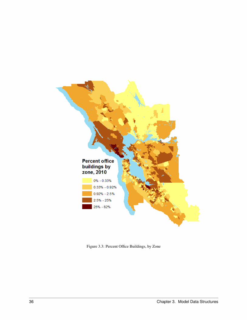
Figure 3.3: Percent Office Buildings, by Zone
36 Chapter 3. Model Data Structures
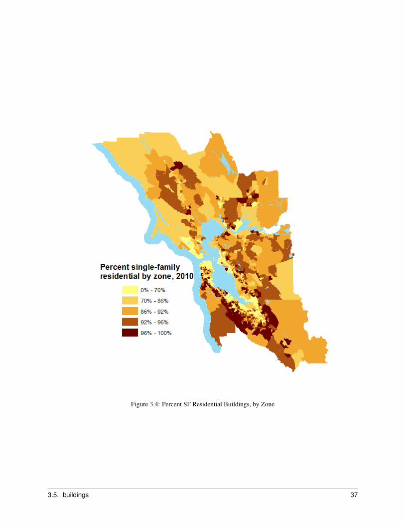
Figure 3.4: Percent SF Residential Buildings, by Zone
3.5. buildings 37

Figure 3.5: Buildings per Acre, by Zone
38 Chapter 3. Model Data Structures
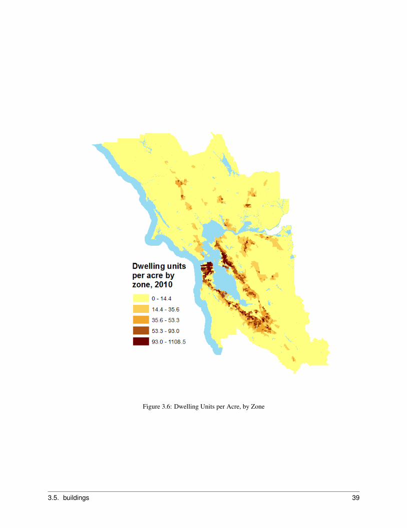
Figure 3.6: Dwelling Units per Acre, by Zone
3.5. buildings 39
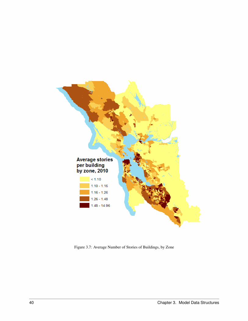
Figure 3.7: Average Number of Stories of Buildings, by Zone
40 Chapter 3. Model Data Structures
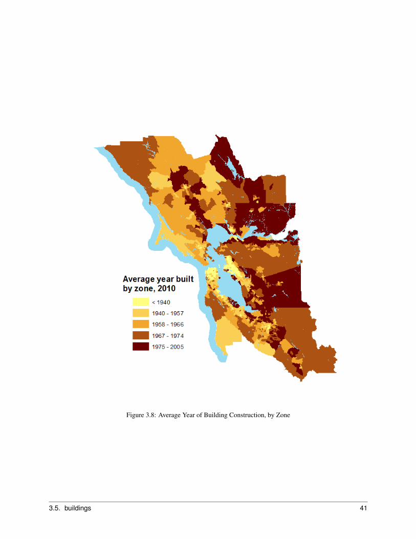
Figure 3.8: Average Year of Building Construction, by Zone
3.5. buildings 41

3.6 building_sqft_per_job
This table contains a listing of the non-residential square footage used by jobs in particular building types. It is usedby the real estate development model, as well as the business location choice model.
A building_sqft_per_job table has been prepared and formatted for UrbanSim.Column Name Data Type Descriptionid integer unique identifieremployment_submarket_id integer the submarket the record applies tobuilding_type_id integer the building type the record applies tobuilding_sqft_per_employee integer the sqft per job each job in a particular building type in a
particular zone
3.7 building_types
The building_types table provides a list of unique building types as classified by ABAG. Separate Real Estate Pricesubmodels may be specified for each type of building.
A building_types table has been prepared and formatted for the Bay Area UrbanSim model system. Curently, 16building types are defined, and it is denoted whether each type ’is residential’ and ’has jobs’ onsite.
Column Name Data Type Descriptionbuilding_type_id integer unique identifierbuilding_type_name varchar name of the building typebuilding_type_short_name varchar abbreviation of the building type nameis_residential boolean 1 if this building type is residential, 0 otherwisehas_residential boolean 1 if this building type has a residential component, 0 otherwise
Column Name Data Type Descriptionbuilding_type_id integer building typesize_category varchardemolition_cost_per_sqft integer cost in dollars per sqft of demolition
3.8 employment_sectors
The employment_sectors table contains categories that represent ABAG-defined aggregations of an industrialclassification (e.g. NAICS or SIC). It is used by the employment models, including the Business Location ChoiceModel, where separate submodels can be specified for each employment sector. Each row in the table defines oneEmployment Sector.
An employment_secors table has been prepared and formatted. 28 sectors are represented (ABAG’s 27-sectordefinition plus unclassified). These categories map directly to NAICS categories, as well as to Census PUMS ACSdefinitions of industry and occupation type. These employment sectors were also selected so as to provide a goodcorrespondence to building type-industry usage categories.
Column Name Data Type Descriptionsector_id integer Unique identifiername varchar Unique name of the Sector
42 Chapter 3. Model Data Structures

3.9 households
The household table contains household data, with each row pertaining to one household. The household table ismodified by the Household Transition Model, the Household Relocation Model, and the Household Location ChoiceModel .
Column Name Data Type Descriptionhousehold_id integer Unique identifierbuilding_id integer Building this household resides in; -1 if currently not residing in a housing unitbuilding_typd_id integer Building type this household resides intenure integer rent (1) vs. own (2)persons integer Total number of people living in this household.workers integer Total number of workers living in this household.age_of_head integer Age of head of the householdincome integer Income of this householdchildren integer Number of children living in this householdrace_id integer Race of head of householdcars integer Number of cars in this household
A household table has been prepared and formatted for UrbanSim. Households in the table were synthesized by MTCfrom Census 2000 PUMS and SF3 tables using the MTC population synthesizer. The households table was thenupdated to reflect observed 2010 data.
2,616,085 households are in the base-year households table. The mean persons per household is 2.7. The meannumber of household workers is 1.39. The mean age of household head is 48.6 years. The mean number of householdvehicles is 1.77. The mean household income is $81,937. The mean number of household children is 0.53.
Figures 3.9 and 3.10 map out selected household table attributes at the zonal level.
3.9. households 43
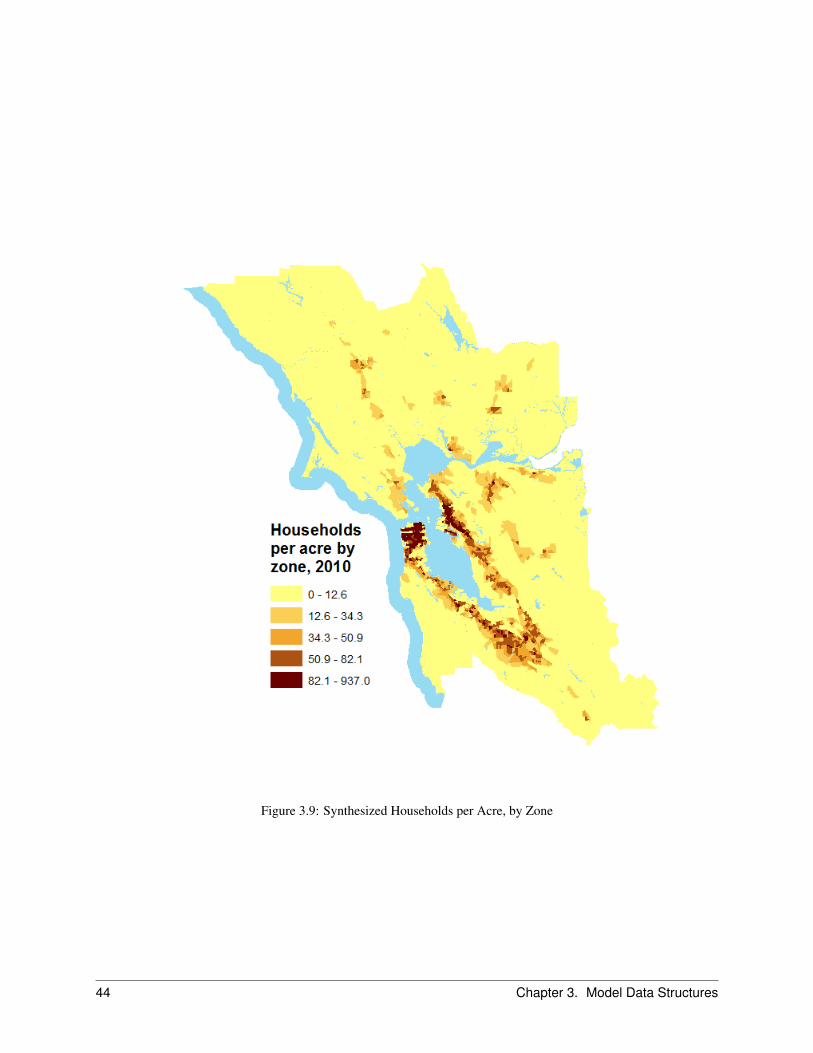
Figure 3.9: Synthesized Households per Acre, by Zone
44 Chapter 3. Model Data Structures
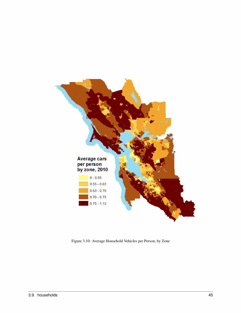
Figure 3.10: Average Household Vehicles per Person, by Zone
3.9. households 45
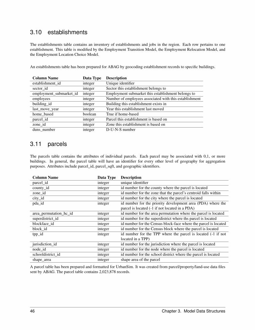
3.10 establishments
The establishments table contains an inventory of establishments and jobs in the region. Each row pertains to oneestablishment. This table is modified by the Employment Transition Model, the Employment Relocation Model, andthe Employment Location Choice Model.
An establishments table has been prepared for ABAG by geocoding establishment records to specific buildings.
Column Name Data Type Descriptionestablishment_id integer Unique identifiersector_id integer Sector this establishment belongs toemployment_submarket_id integer Employment submarket this establishment belongs toemployees integer Number of employees associated with this establishmentbuilding_id integer Building this establishment exists inlast_move_year integer Year this establishment last movedhome_based boolean True if home-basedparcel_id integer Parcel this establishment is based onzone_id integer Zone this establishment is based onduns_number integer D-U-N-S number
3.11 parcels
The parcels table contains the attributes of individual parcels. Each parcel may be associated with 0,1, or morebuildings. In general, the parcel table will have an identifier for every other level of geography for aggregationpurposes. Attributes include parcel_id, parcel_sqft, and geographic identifiers.
Column Name Data Type Descriptionparcel_id integer unique identifiercounty_id integer id number for the county where the parcel is locatedzone_id integer id number for the zone that the parcel’s centroid falls withincity_id integer id number for the city where the parcel is locatedpda_id integer id number for the priority development area (PDA) where the
parcel is located (-1 if not located in a PDA)area_permutation_hc_id integer id number for the area permutation where the parcel is locatedsuperdistrict_id integer id number for the superdistrict where ths parcel is locatedblockface_id integer id number for the Census block-face where the parcel is locatedblock_id integer id number for the Census block where the parcel is locatedtpp_id integer id number for the TPP where the parcel is located (-1 if not
located in a TPP)jurisdiction_id integer id number for the jurisdiction where the parcel is locatednode_id integer id number for the node where the parcel is locatedschooldistrict_id integer id number for the school district where the parcel is locatedshape_area integer shape area of the parcel
A parcel table has been prepared and formatted for UrbanSim. It was created from parcel/property/land-use data filessent by ABAG. The parcel table contains 2,023,878 records.
46 Chapter 3. Model Data Structures
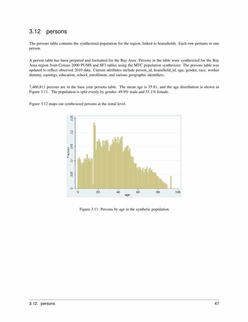
3.12 persons
The persons table contains the synthesized population for the region, linked to households. Each row pertains to oneperson.
A person table has been prepared and formatted for the Bay Area. Persons in the table were synthesized for the BayArea region from Census 2000 PUMS and SF3 tables using the MTC population synthesizer. The persons table wasupdated to reflect observed 2010 data. Current attributes include person_id, household_id, age, gender, race, workerdummy, earnings, education, school_enrollment, and various geographic identifiers.
7,460,811 persons are in the base year persons table. The mean age is 35.81, and the age distribution is shown inFigure 3.11 . The population is split evenly by gender- 49.9% male and 51.1% female.
Figure 3.12 maps out synthesized persons at the zonal level.
Figure 3.11: Persons by age in the synthetic population
3.12. persons 47
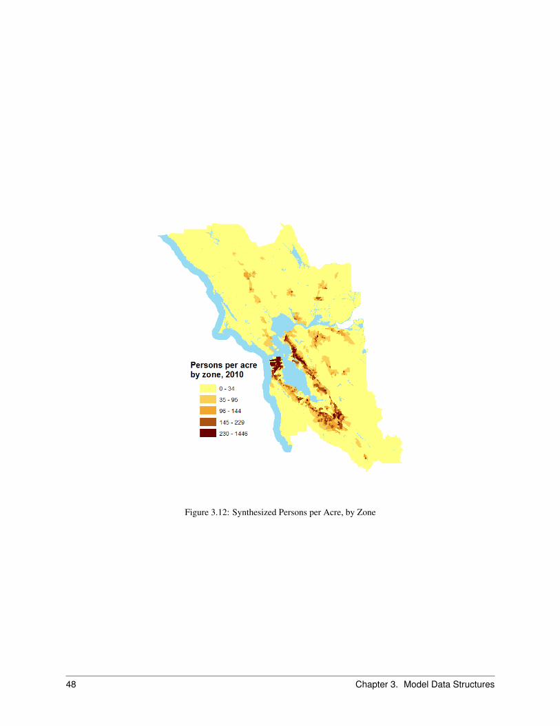
Figure 3.12: Synthesized Persons per Acre, by Zone
48 Chapter 3. Model Data Structures

3.13 geography_zoning
The geography_zoning table (a database table that is not cached) contains the list of zoning designations, reflectingsome classification of land use regulations defining permissible uses and densities of future development. Each recordin the table represents a set of rules that restrict development in specific ways. It is used by the the developer modelto determine what buildings can be constructed on each parcel. Table attributes include maximum FAR, maximumbuilding height, front/side/rear setbacks, minimum lot size, and maximum parcel coverage.
Column Name Data Type Descriptionid integer Unique zoning identification numbername string (14) Name of zoning classificationmin_far float Minimum FAR, if applicablemax_far float Maximum FAR, if applicablemax_height float Maximum building height in feetmin_dua float Minimum residential units per acre, if applicablemax_dua float Maximum residential units per acre, if applicablemin_lot_size float Minimum lot size in square feetcoverage float Maximum proportion of parcel land area that can be developedmax_du_per_parcel float Maximum number of residential units that can be built per par-
celmin_front_setback float Minimum building setback from front of parcel, in feetmax_front_setback float Maximum building setback from front of parcel, in feetside_setback float Minimum building setback from sides of parcel, in feetrear_setback float Minimum building setback from rear of parcel, in feetcity integer Id of city where zoning classification is applicable
3.14 geography_building_type_zone_relation
The geography_building_type_zone_relation table specifies the allowable building types that may be constructed ineach zoning category found in the geography_zoning table. Each row represents one zoning-category/building-typepair.
Column Name Data Type Descriptionzoning_id integer a zoning id from plan_types tablebuilding_type integer a building type id from the building_types table
3.15 zone_accessibility
The zone_accessibility table contains zonal accessibility variables. It is used to store travel-model generatedaccessibility variables used by various models.
This table can be updated with the results of any travel model run.
Column Name Data Type Descriptionzone_id integer Unique identifier
3.13. geography_zoning 49

3.16 zones
The zones table contains a list of traffic analysis zones used in the travel model. The current 1454 ABAG/ MTC zonesystem is used. Characteristics of each zone are also added to this table.
Column Name Data Type Descriptionzone_id integer Unique identifier
50 Chapter 3. Model Data Structures

CHAPTER
FOUR
Model Estimation for the Bay Area
This chapter documents the specification, estimation, calibration and validation of the UrbanSim model componentsfor the Bay Area region. The first sections present model estimation results. This is organized according to thedifferent UrbanSim models that require statistical estimation of parameters. For each model, model structure anddata are briefly reviewed, followed by a description of the model specification and estimation results for the modelequations. All estimated coefficients were generated within UrbanSim.
After estimation results are presented, the calibration and validation process is discussed. Model estimation wasfollowed by 1-year simulation runs to compare output with validation targets. Models were calibrated in order tobetter account for target changes. Next, 30-year simulations were run to gauge the model’s policy sensitivities. Modelcalibration, validation, and sensitivity analyses were highly inter-connected procedures, due to UrbanSim modelcomponents having a high degree of mutual influence. Adjusting one model might necessitate the re-calibration of aseparate model; the whole process was iterative and inter-dependent.
4.1 Household Location Choice
The Household Location Choice Model (HLCM) predicts the probability that a household that is either new(from the Household Transition model) or has decided to move within the region (from the Household Relocationmodel) will choose a particular submarket location. The model is specified as a multinomial logit (MNL) withsampling of alternatives from the universe of submarkets to estimate model coefficients. Submarkets are defined asschool-district/residential-building-type/tenure/transit-proximity combinations. After submarkets are predicted forhouseholds (using Monte Carlo simulation), the choice of a specific building within the submarket is predicted.
The model is stratified into submodels by household income, size, and tenure (4 income categories, 3 household sizecategories, and 2 tenure categories, for a total of 24 submodels). Explanatory variables used in the model includeaccessibility, attributes of housing, price, and interaction terms between household and location attributes.
The location choice set consists of submarket alternatives. Submarkets are defined by school district, residentialbuilding type, tenure, and transit proximity combinations. The submarket dataset is automatically generated fromthe parcel-level building data, so the number of submarkets in the region can evolve over time if areas take on newbuilding types.
Model coefficients were estimated using data from the synthetic households table for the Bay Area. For the majorityof submodels (except when the sample size was too small), only households that had moved within the previous fiveyears (as identified in the PUMS record) were used for estimation. The restriction to households which had movedwithin the past 5 years was made to reflect the choices of households in similar circumstances to those being modeled(household that are relocating or moving into the region).
51

Household location choice is represented for the Bay Area by a sequence of choice models. The models are, in order:tenure choice, submarket choice, and building choice. This is the order in which the models are simulated. The firstchoice model represents a binary household choice of ’rent’ vs. ’own’. Tenure model coefficients are shown in Table4.1. Next, the choice of submarket is modeled, conditional on the previously modeled tenure dimension. Tables 4.2to 4.25 below list the coefficients for the submodels, each of which was specified independently. Variable sets weresomewhat similar across submodels, although there was variation owing to the principal that households in differentsumbmodels might predicate their location choice on different factors. The final model in the sequence of models thatrepresents household location choice is a simple location choice model that allocates households to specific buildingswithin the chosen submarket.
In the tenure choice model, children, age of head, and income are hypothesized to be positively associated withhome-ownership. In the submarket household locaation choice models, the location choice of owner-householdsis hypothesized to be positively associated with single-family submarkets (and the opposite association is likelyto be seen for renters), a negative association with price is hypothesized across all submodels, and, other thingsequal,a positive association with accessibility, square footage, residential units, and income is hypothesized acrossall submodels. For some variables, variation in coefficient sign is expected, as the correlations between householdlocation choice and specific variables will vary by submodel (recall that submodels reflect household income, size,and tenure categories) and in some cases variables may be proxying for the effect of an unobserved variable.
52 Chapter 4. Model Estimation for the Bay Area
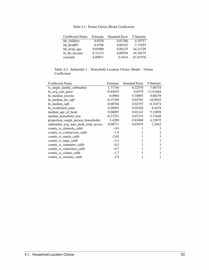
Table 4.1: Tenure Choice Model Coefficients
Coefficient Name Estimate Standard Error T-Statistichh_children 0.0528 0.01286 4.10757hh_head65 -0.4766 0.06162 -7.73455hh_head_age 0.05988 0.00135 44.21329ln_hh_income 0.31233 0.00704 44.38535constant -4.80851 0.1014 -47.41976
Table 4.2: Submodel 1 - Household Location Choice Model - OwnerCoefficients
Coefficient Name Estimate Standard Error T-Statisticis_single_family_submarket 1.71744 0.22576 7.60734ln_avg_sale_price -0.44035 0.0379 -11.61844ln_median_income 0.0964 0.16003 0.60239ln_median_lot_sqft -0.37356 0.03701 -10.0943ln_median_sqft -0.00764 0.02353 -0.32474ln_residential_units 0.20493 0.02426 8.4478median_age_of_head 0.06093 0.01141 5.33858median_household_size -0.27251 0.07333 -3.71648proportion_single_person_households 3.4289 0.81048 4.23072submarket_avg_auto_peak_total_access 0.08771 0.03979 2.2043county_is_alameda_calib -0.9 1 1county_is_contracosta_calib -1.8 1 1county_is_marin_calib -2.65 1 1county_is_napa_calib -2.4 1 1county_is_sanmateo_calib -0.5 1 1county_is_santaclara_calib -0.7 1 1county_is_solano_calib -1.7 1 1county_is_sonoma_calib -2.9 1 1
4.1. Household Location Choice 53
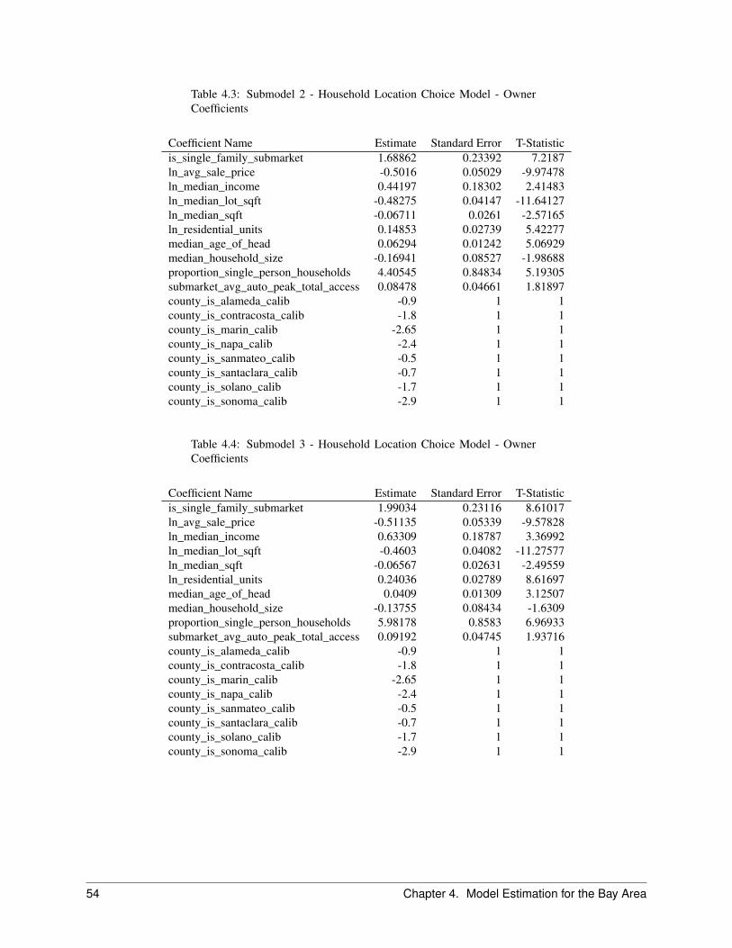
Table 4.3: Submodel 2 - Household Location Choice Model - OwnerCoefficients
Coefficient Name Estimate Standard Error T-Statisticis_single_family_submarket 1.68862 0.23392 7.2187ln_avg_sale_price -0.5016 0.05029 -9.97478ln_median_income 0.44197 0.18302 2.41483ln_median_lot_sqft -0.48275 0.04147 -11.64127ln_median_sqft -0.06711 0.0261 -2.57165ln_residential_units 0.14853 0.02739 5.42277median_age_of_head 0.06294 0.01242 5.06929median_household_size -0.16941 0.08527 -1.98688proportion_single_person_households 4.40545 0.84834 5.19305submarket_avg_auto_peak_total_access 0.08478 0.04661 1.81897county_is_alameda_calib -0.9 1 1county_is_contracosta_calib -1.8 1 1county_is_marin_calib -2.65 1 1county_is_napa_calib -2.4 1 1county_is_sanmateo_calib -0.5 1 1county_is_santaclara_calib -0.7 1 1county_is_solano_calib -1.7 1 1county_is_sonoma_calib -2.9 1 1
Table 4.4: Submodel 3 - Household Location Choice Model - OwnerCoefficients
Coefficient Name Estimate Standard Error T-Statisticis_single_family_submarket 1.99034 0.23116 8.61017ln_avg_sale_price -0.51135 0.05339 -9.57828ln_median_income 0.63309 0.18787 3.36992ln_median_lot_sqft -0.4603 0.04082 -11.27577ln_median_sqft -0.06567 0.02631 -2.49559ln_residential_units 0.24036 0.02789 8.61697median_age_of_head 0.0409 0.01309 3.12507median_household_size -0.13755 0.08434 -1.6309proportion_single_person_households 5.98178 0.8583 6.96933submarket_avg_auto_peak_total_access 0.09192 0.04745 1.93716county_is_alameda_calib -0.9 1 1county_is_contracosta_calib -1.8 1 1county_is_marin_calib -2.65 1 1county_is_napa_calib -2.4 1 1county_is_sanmateo_calib -0.5 1 1county_is_santaclara_calib -0.7 1 1county_is_solano_calib -1.7 1 1county_is_sonoma_calib -2.9 1 1
54 Chapter 4. Model Estimation for the Bay Area
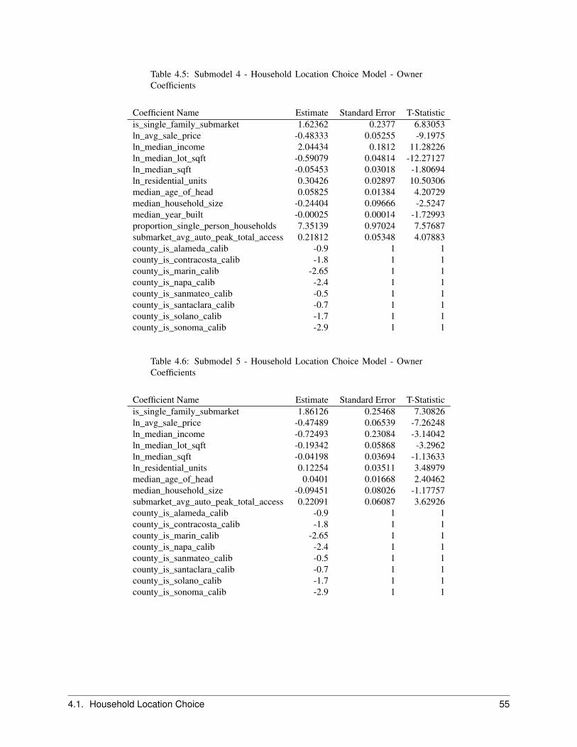
Table 4.5: Submodel 4 - Household Location Choice Model - OwnerCoefficients
Coefficient Name Estimate Standard Error T-Statisticis_single_family_submarket 1.62362 0.2377 6.83053ln_avg_sale_price -0.48333 0.05255 -9.1975ln_median_income 2.04434 0.1812 11.28226ln_median_lot_sqft -0.59079 0.04814 -12.27127ln_median_sqft -0.05453 0.03018 -1.80694ln_residential_units 0.30426 0.02897 10.50306median_age_of_head 0.05825 0.01384 4.20729median_household_size -0.24404 0.09666 -2.5247median_year_built -0.00025 0.00014 -1.72993proportion_single_person_households 7.35139 0.97024 7.57687submarket_avg_auto_peak_total_access 0.21812 0.05348 4.07883county_is_alameda_calib -0.9 1 1county_is_contracosta_calib -1.8 1 1county_is_marin_calib -2.65 1 1county_is_napa_calib -2.4 1 1county_is_sanmateo_calib -0.5 1 1county_is_santaclara_calib -0.7 1 1county_is_solano_calib -1.7 1 1county_is_sonoma_calib -2.9 1 1
Table 4.6: Submodel 5 - Household Location Choice Model - OwnerCoefficients
Coefficient Name Estimate Standard Error T-Statisticis_single_family_submarket 1.86126 0.25468 7.30826ln_avg_sale_price -0.47489 0.06539 -7.26248ln_median_income -0.72493 0.23084 -3.14042ln_median_lot_sqft -0.19342 0.05868 -3.2962ln_median_sqft -0.04198 0.03694 -1.13633ln_residential_units 0.12254 0.03511 3.48979median_age_of_head 0.0401 0.01668 2.40462median_household_size -0.09451 0.08026 -1.17757submarket_avg_auto_peak_total_access 0.22091 0.06087 3.62926county_is_alameda_calib -0.9 1 1county_is_contracosta_calib -1.8 1 1county_is_marin_calib -2.65 1 1county_is_napa_calib -2.4 1 1county_is_sanmateo_calib -0.5 1 1county_is_santaclara_calib -0.7 1 1county_is_solano_calib -1.7 1 1county_is_sonoma_calib -2.9 1 1
4.1. Household Location Choice 55
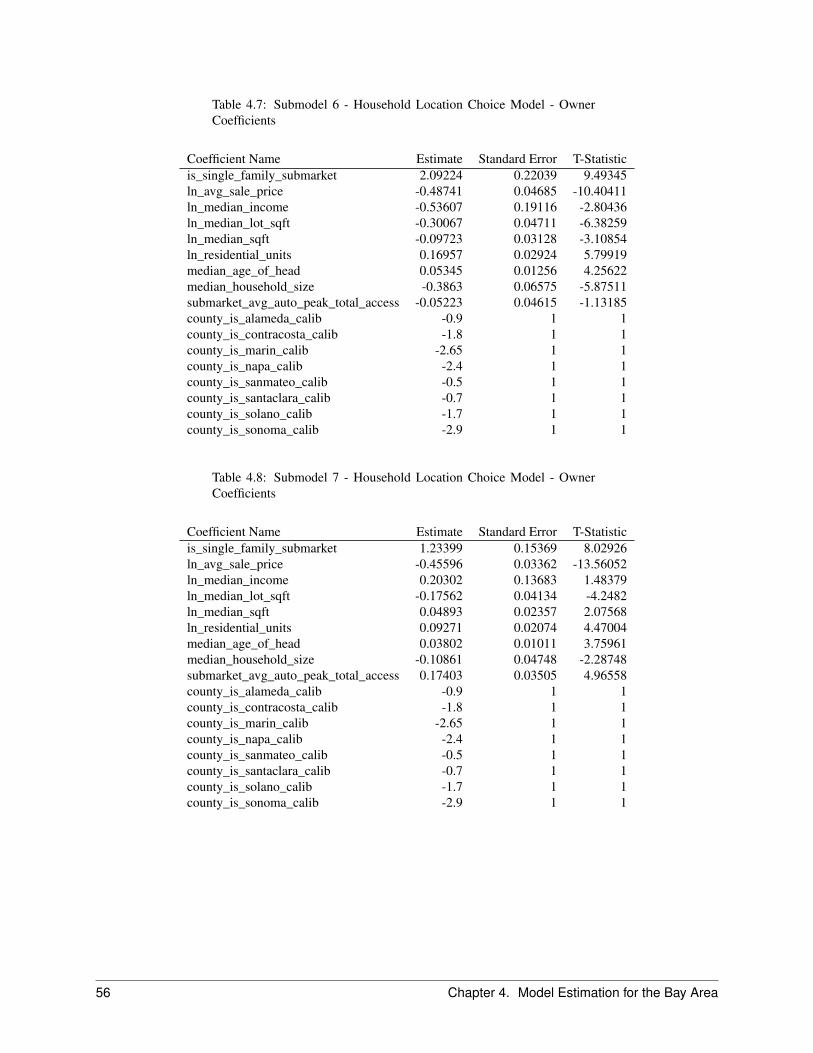
Table 4.7: Submodel 6 - Household Location Choice Model - OwnerCoefficients
Coefficient Name Estimate Standard Error T-Statisticis_single_family_submarket 2.09224 0.22039 9.49345ln_avg_sale_price -0.48741 0.04685 -10.40411ln_median_income -0.53607 0.19116 -2.80436ln_median_lot_sqft -0.30067 0.04711 -6.38259ln_median_sqft -0.09723 0.03128 -3.10854ln_residential_units 0.16957 0.02924 5.79919median_age_of_head 0.05345 0.01256 4.25622median_household_size -0.3863 0.06575 -5.87511submarket_avg_auto_peak_total_access -0.05223 0.04615 -1.13185county_is_alameda_calib -0.9 1 1county_is_contracosta_calib -1.8 1 1county_is_marin_calib -2.65 1 1county_is_napa_calib -2.4 1 1county_is_sanmateo_calib -0.5 1 1county_is_santaclara_calib -0.7 1 1county_is_solano_calib -1.7 1 1county_is_sonoma_calib -2.9 1 1
Table 4.8: Submodel 7 - Household Location Choice Model - OwnerCoefficients
Coefficient Name Estimate Standard Error T-Statisticis_single_family_submarket 1.23399 0.15369 8.02926ln_avg_sale_price -0.45596 0.03362 -13.56052ln_median_income 0.20302 0.13683 1.48379ln_median_lot_sqft -0.17562 0.04134 -4.2482ln_median_sqft 0.04893 0.02357 2.07568ln_residential_units 0.09271 0.02074 4.47004median_age_of_head 0.03802 0.01011 3.75961median_household_size -0.10861 0.04748 -2.28748submarket_avg_auto_peak_total_access 0.17403 0.03505 4.96558county_is_alameda_calib -0.9 1 1county_is_contracosta_calib -1.8 1 1county_is_marin_calib -2.65 1 1county_is_napa_calib -2.4 1 1county_is_sanmateo_calib -0.5 1 1county_is_santaclara_calib -0.7 1 1county_is_solano_calib -1.7 1 1county_is_sonoma_calib -2.9 1 1
56 Chapter 4. Model Estimation for the Bay Area
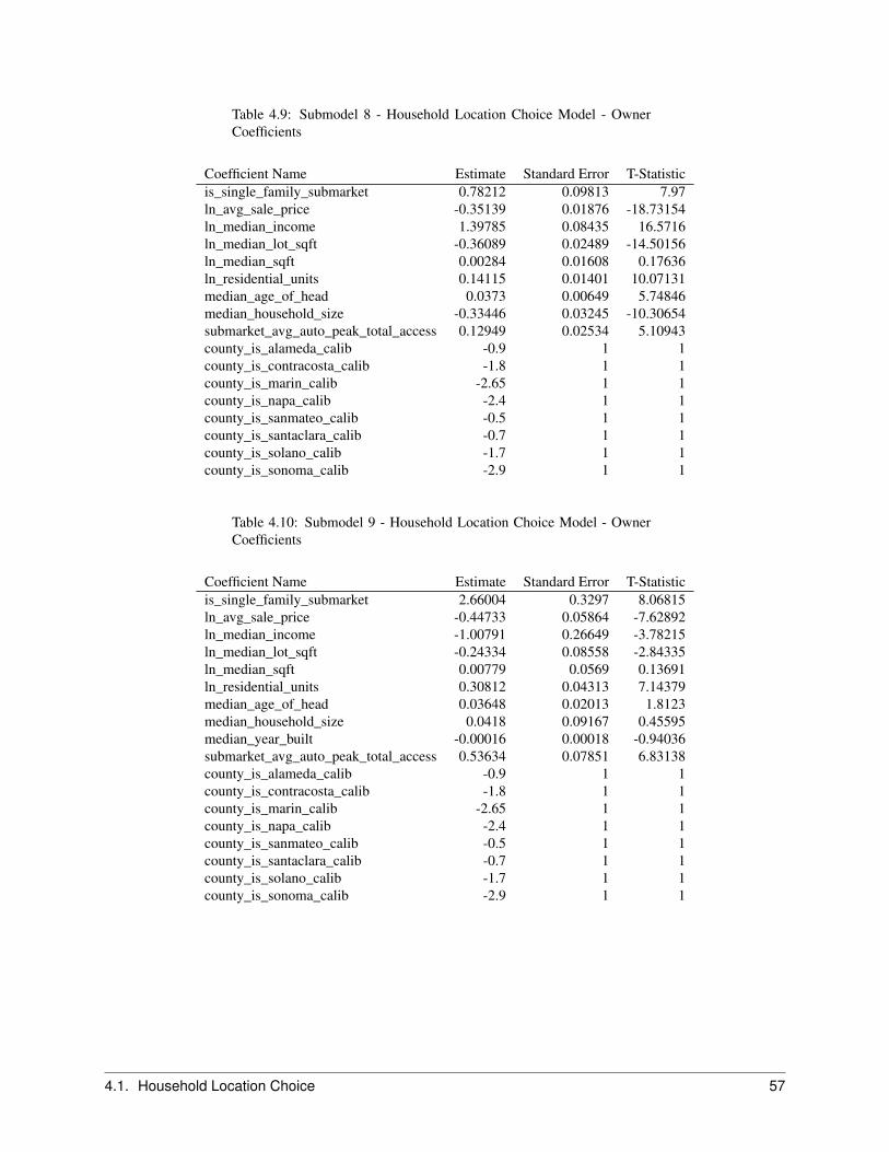
Table 4.9: Submodel 8 - Household Location Choice Model - OwnerCoefficients
Coefficient Name Estimate Standard Error T-Statisticis_single_family_submarket 0.78212 0.09813 7.97ln_avg_sale_price -0.35139 0.01876 -18.73154ln_median_income 1.39785 0.08435 16.5716ln_median_lot_sqft -0.36089 0.02489 -14.50156ln_median_sqft 0.00284 0.01608 0.17636ln_residential_units 0.14115 0.01401 10.07131median_age_of_head 0.0373 0.00649 5.74846median_household_size -0.33446 0.03245 -10.30654submarket_avg_auto_peak_total_access 0.12949 0.02534 5.10943county_is_alameda_calib -0.9 1 1county_is_contracosta_calib -1.8 1 1county_is_marin_calib -2.65 1 1county_is_napa_calib -2.4 1 1county_is_sanmateo_calib -0.5 1 1county_is_santaclara_calib -0.7 1 1county_is_solano_calib -1.7 1 1county_is_sonoma_calib -2.9 1 1
Table 4.10: Submodel 9 - Household Location Choice Model - OwnerCoefficients
Coefficient Name Estimate Standard Error T-Statisticis_single_family_submarket 2.66004 0.3297 8.06815ln_avg_sale_price -0.44733 0.05864 -7.62892ln_median_income -1.00791 0.26649 -3.78215ln_median_lot_sqft -0.24334 0.08558 -2.84335ln_median_sqft 0.00779 0.0569 0.13691ln_residential_units 0.30812 0.04313 7.14379median_age_of_head 0.03648 0.02013 1.8123median_household_size 0.0418 0.09167 0.45595median_year_built -0.00016 0.00018 -0.94036submarket_avg_auto_peak_total_access 0.53634 0.07851 6.83138county_is_alameda_calib -0.9 1 1county_is_contracosta_calib -1.8 1 1county_is_marin_calib -2.65 1 1county_is_napa_calib -2.4 1 1county_is_sanmateo_calib -0.5 1 1county_is_santaclara_calib -0.7 1 1county_is_solano_calib -1.7 1 1county_is_sonoma_calib -2.9 1 1
4.1. Household Location Choice 57
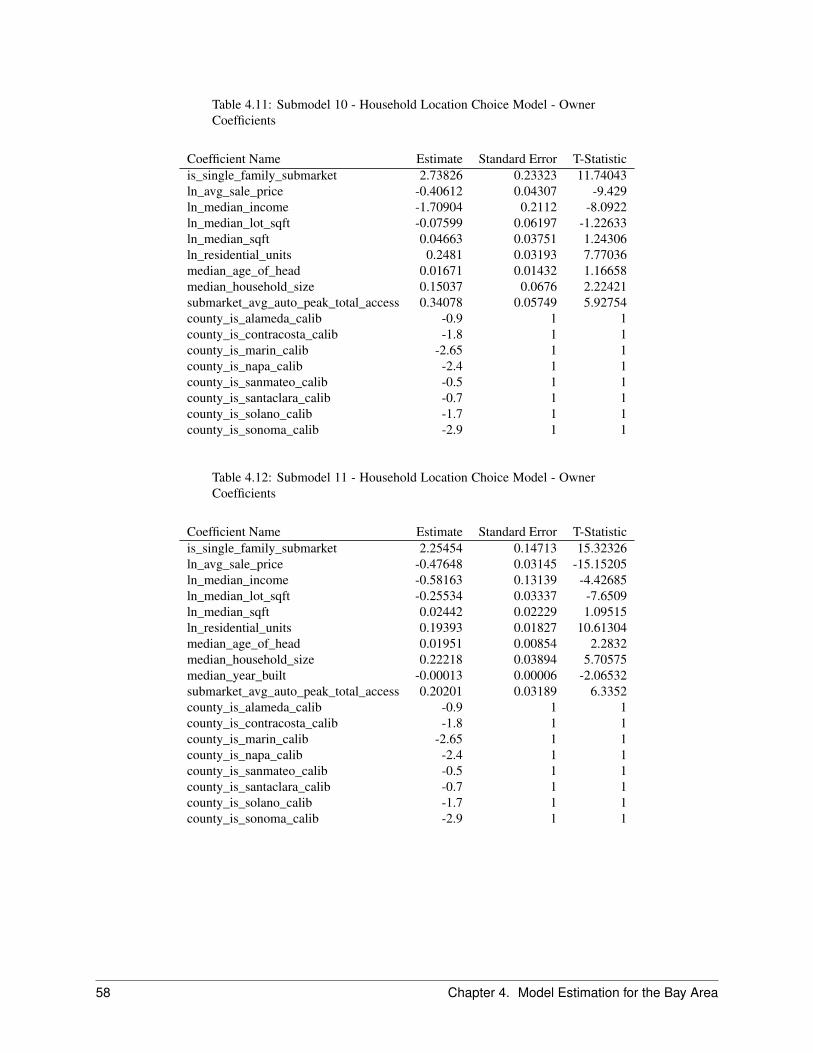
Table 4.11: Submodel 10 - Household Location Choice Model - OwnerCoefficients
Coefficient Name Estimate Standard Error T-Statisticis_single_family_submarket 2.73826 0.23323 11.74043ln_avg_sale_price -0.40612 0.04307 -9.429ln_median_income -1.70904 0.2112 -8.0922ln_median_lot_sqft -0.07599 0.06197 -1.22633ln_median_sqft 0.04663 0.03751 1.24306ln_residential_units 0.2481 0.03193 7.77036median_age_of_head 0.01671 0.01432 1.16658median_household_size 0.15037 0.0676 2.22421submarket_avg_auto_peak_total_access 0.34078 0.05749 5.92754county_is_alameda_calib -0.9 1 1county_is_contracosta_calib -1.8 1 1county_is_marin_calib -2.65 1 1county_is_napa_calib -2.4 1 1county_is_sanmateo_calib -0.5 1 1county_is_santaclara_calib -0.7 1 1county_is_solano_calib -1.7 1 1county_is_sonoma_calib -2.9 1 1
Table 4.12: Submodel 11 - Household Location Choice Model - OwnerCoefficients
Coefficient Name Estimate Standard Error T-Statisticis_single_family_submarket 2.25454 0.14713 15.32326ln_avg_sale_price -0.47648 0.03145 -15.15205ln_median_income -0.58163 0.13139 -4.42685ln_median_lot_sqft -0.25534 0.03337 -7.6509ln_median_sqft 0.02442 0.02229 1.09515ln_residential_units 0.19393 0.01827 10.61304median_age_of_head 0.01951 0.00854 2.2832median_household_size 0.22218 0.03894 5.70575median_year_built -0.00013 0.00006 -2.06532submarket_avg_auto_peak_total_access 0.20201 0.03189 6.3352county_is_alameda_calib -0.9 1 1county_is_contracosta_calib -1.8 1 1county_is_marin_calib -2.65 1 1county_is_napa_calib -2.4 1 1county_is_sanmateo_calib -0.5 1 1county_is_santaclara_calib -0.7 1 1county_is_solano_calib -1.7 1 1county_is_sonoma_calib -2.9 1 1
58 Chapter 4. Model Estimation for the Bay Area
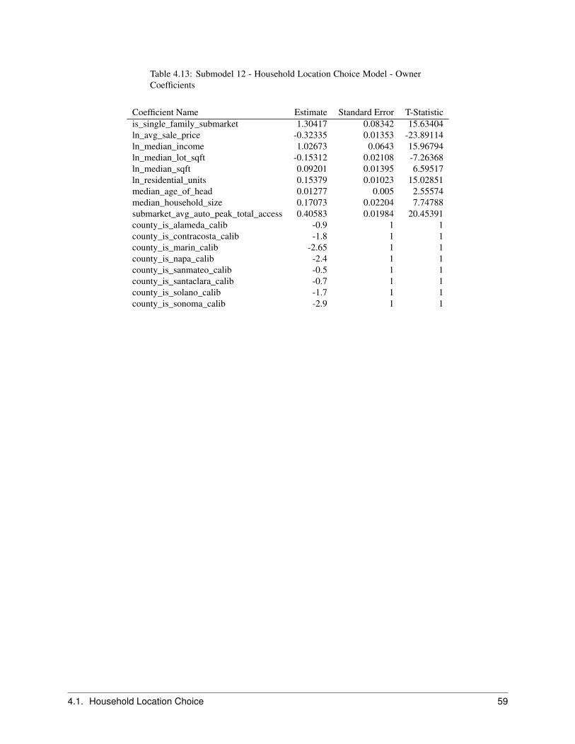
Table 4.13: Submodel 12 - Household Location Choice Model - OwnerCoefficients
Coefficient Name Estimate Standard Error T-Statisticis_single_family_submarket 1.30417 0.08342 15.63404ln_avg_sale_price -0.32335 0.01353 -23.89114ln_median_income 1.02673 0.0643 15.96794ln_median_lot_sqft -0.15312 0.02108 -7.26368ln_median_sqft 0.09201 0.01395 6.59517ln_residential_units 0.15379 0.01023 15.02851median_age_of_head 0.01277 0.005 2.55574median_household_size 0.17073 0.02204 7.74788submarket_avg_auto_peak_total_access 0.40583 0.01984 20.45391county_is_alameda_calib -0.9 1 1county_is_contracosta_calib -1.8 1 1county_is_marin_calib -2.65 1 1county_is_napa_calib -2.4 1 1county_is_sanmateo_calib -0.5 1 1county_is_santaclara_calib -0.7 1 1county_is_solano_calib -1.7 1 1county_is_sonoma_calib -2.9 1 1
4.1. Household Location Choice 59
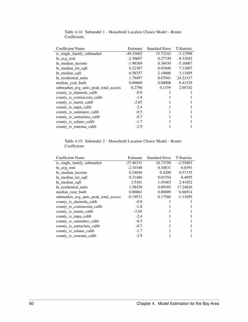
Table 4.14: Submodel 1 - Household Location Choice Model - RenterCoefficients
Coefficient Name Estimate Standard Error T-Statisticis_single_family_submarket -49.33662 15.73242 -3.13598ln_avg_rent -2.30607 0.27749 -8.31042ln_median_income -1.98369 0.38439 -5.16067ln_median_lot_sqft 0.22307 0.03048 7.31807ln_median_sqft 6.58357 2.10006 3.13495ln_residential_units 1.70497 0.07041 24.21317median_year_built 0.00069 0.00008 8.41329submarket_avg_auto_peak_total_access 0.2796 0.1359 2.05742county_is_alameda_calib -0.9 1 1county_is_contracosta_calib -1.8 1 1county_is_marin_calib -2.65 1 1county_is_napa_calib -2.4 1 1county_is_sanmateo_calib -0.5 1 1county_is_santaclara_calib -0.7 1 1county_is_solano_calib -1.7 1 1county_is_sonoma_calib -2.9 1 1
Table 4.15: Submodel 2 - Household Location Choice Model - RenterCoefficients
Coefficient Name Estimate Standard Error T-Statisticis_single_family_submarket -27.46331 10.73358 -2.55863ln_avg_rent -2.10348 0.34831 -6.0391ln_median_income 0.24048 0.4209 0.57135ln_median_lot_sqft 0.21486 0.03354 6.4055ln_median_sqft 3.5181 1.45465 2.41852ln_residential_units 1.58428 0.09185 17.24826median_year_built 0.00061 0.00009 6.66914submarket_avg_auto_peak_total_access -0.19531 0.17586 -1.11059county_is_alameda_calib -0.9 1 1county_is_contracosta_calib -1.8 1 1county_is_marin_calib -2.65 1 1county_is_napa_calib -2.4 1 1county_is_sanmateo_calib -0.5 1 1county_is_santaclara_calib -0.7 1 1county_is_solano_calib -1.7 1 1county_is_sonoma_calib -2.9 1 1
60 Chapter 4. Model Estimation for the Bay Area

Table 4.16: Submodel 3 - Household Location Choice Model - RenterCoefficients
Coefficient Name Estimate Standard Error T-Statisticis_single_family_submarket -82.94025 29.46636 -2.81474ln_avg_rent -3.1692 0.54009 -5.8679ln_median_income 2.46983 0.5995 4.1198ln_median_lot_sqft 0.20346 0.05528 3.68034ln_median_sqft 10.69258 3.95712 2.70211ln_residential_units 1.58801 0.12393 12.81378median_year_built 0.00065 0.00013 5.17189submarket_avg_auto_peak_total_access -0.17919 0.25707 -0.69705county_is_alameda_calib -0.9 1 1county_is_contracosta_calib -1.8 1 1county_is_marin_calib -2.65 1 1county_is_napa_calib -2.4 1 1county_is_sanmateo_calib -0.5 1 1county_is_santaclara_calib -0.7 1 1county_is_solano_calib -1.7 1 1county_is_sonoma_calib -2.9 1 1
Table 4.17: Submodel 4 - Household Location Choice Model - RenterCoefficients
Coefficient Name Estimate Standard Error T-Statisticis_single_family_submarket -7.03252 0.468 -15.02671ln_avg_rent -2.15289 0.20801 -10.35004ln_median_income 2.86519 0.42658 6.71668ln_median_lot_sqft 0.87813 0.04447 19.74783ln_residential_units 1.41582 0.11348 12.47614median_year_built 0.00337 0.00013 25.45209submarket_avg_auto_peak_total_access -0.4502 0.26289 -1.71251county_is_alameda_calib -0.9 1 1county_is_contracosta_calib -1.8 1 1county_is_marin_calib -2.65 1 1county_is_napa_calib -2.4 1 1county_is_sanmateo_calib -0.5 1 1county_is_santaclara_calib -0.7 1 1county_is_solano_calib -1.7 1 1county_is_sonoma_calib -2.9 1 1
4.1. Household Location Choice 61
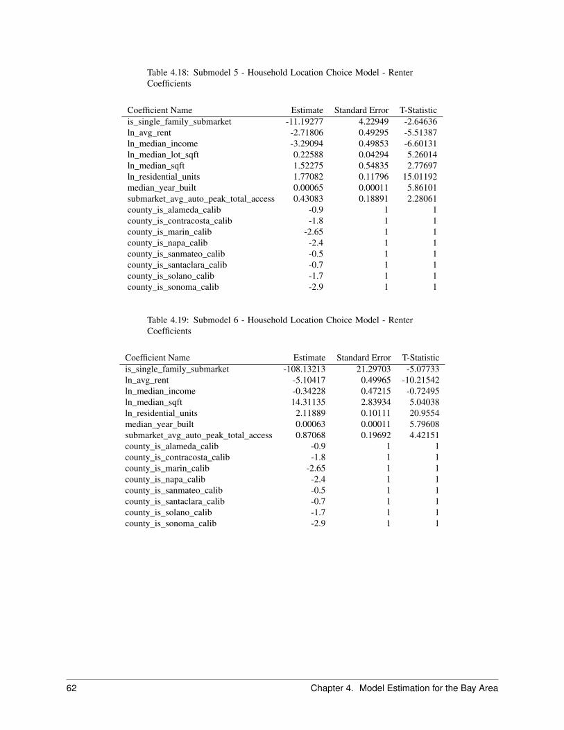
Table 4.18: Submodel 5 - Household Location Choice Model - RenterCoefficients
Coefficient Name Estimate Standard Error T-Statisticis_single_family_submarket -11.19277 4.22949 -2.64636ln_avg_rent -2.71806 0.49295 -5.51387ln_median_income -3.29094 0.49853 -6.60131ln_median_lot_sqft 0.22588 0.04294 5.26014ln_median_sqft 1.52275 0.54835 2.77697ln_residential_units 1.77082 0.11796 15.01192median_year_built 0.00065 0.00011 5.86101submarket_avg_auto_peak_total_access 0.43083 0.18891 2.28061county_is_alameda_calib -0.9 1 1county_is_contracosta_calib -1.8 1 1county_is_marin_calib -2.65 1 1county_is_napa_calib -2.4 1 1county_is_sanmateo_calib -0.5 1 1county_is_santaclara_calib -0.7 1 1county_is_solano_calib -1.7 1 1county_is_sonoma_calib -2.9 1 1
Table 4.19: Submodel 6 - Household Location Choice Model - RenterCoefficients
Coefficient Name Estimate Standard Error T-Statisticis_single_family_submarket -108.13213 21.29703 -5.07733ln_avg_rent -5.10417 0.49965 -10.21542ln_median_income -0.34228 0.47215 -0.72495ln_median_sqft 14.31135 2.83934 5.04038ln_residential_units 2.11889 0.10111 20.9554median_year_built 0.00063 0.00011 5.79608submarket_avg_auto_peak_total_access 0.87068 0.19692 4.42151county_is_alameda_calib -0.9 1 1county_is_contracosta_calib -1.8 1 1county_is_marin_calib -2.65 1 1county_is_napa_calib -2.4 1 1county_is_sanmateo_calib -0.5 1 1county_is_santaclara_calib -0.7 1 1county_is_solano_calib -1.7 1 1county_is_sonoma_calib -2.9 1 1
62 Chapter 4. Model Estimation for the Bay Area
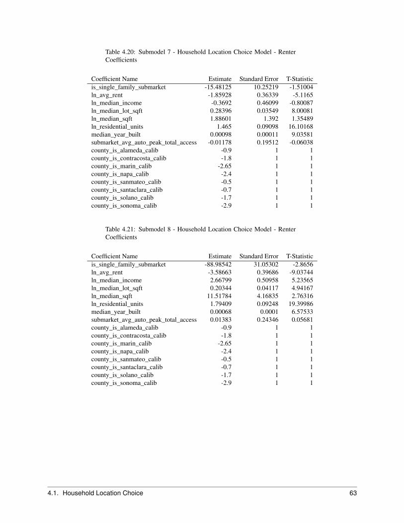
Table 4.20: Submodel 7 - Household Location Choice Model - RenterCoefficients
Coefficient Name Estimate Standard Error T-Statisticis_single_family_submarket -15.48125 10.25219 -1.51004ln_avg_rent -1.85928 0.36339 -5.1165ln_median_income -0.3692 0.46099 -0.80087ln_median_lot_sqft 0.28396 0.03549 8.00081ln_median_sqft 1.88601 1.392 1.35489ln_residential_units 1.465 0.09098 16.10168median_year_built 0.00098 0.00011 9.03581submarket_avg_auto_peak_total_access -0.01178 0.19512 -0.06038county_is_alameda_calib -0.9 1 1county_is_contracosta_calib -1.8 1 1county_is_marin_calib -2.65 1 1county_is_napa_calib -2.4 1 1county_is_sanmateo_calib -0.5 1 1county_is_santaclara_calib -0.7 1 1county_is_solano_calib -1.7 1 1county_is_sonoma_calib -2.9 1 1
Table 4.21: Submodel 8 - Household Location Choice Model - RenterCoefficients
Coefficient Name Estimate Standard Error T-Statisticis_single_family_submarket -88.98542 31.05302 -2.8656ln_avg_rent -3.58663 0.39686 -9.03744ln_median_income 2.66799 0.50958 5.23565ln_median_lot_sqft 0.20344 0.04117 4.94167ln_median_sqft 11.51784 4.16835 2.76316ln_residential_units 1.79409 0.09248 19.39986median_year_built 0.00068 0.0001 6.57533submarket_avg_auto_peak_total_access 0.01383 0.24346 0.05681county_is_alameda_calib -0.9 1 1county_is_contracosta_calib -1.8 1 1county_is_marin_calib -2.65 1 1county_is_napa_calib -2.4 1 1county_is_sanmateo_calib -0.5 1 1county_is_santaclara_calib -0.7 1 1county_is_solano_calib -1.7 1 1county_is_sonoma_calib -2.9 1 1
4.1. Household Location Choice 63
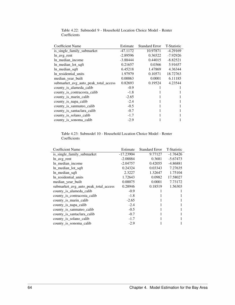
Table 4.22: Submodel 9 - Household Location Choice Model - RenterCoefficients
Coefficient Name Estimate Standard Error T-Statisticis_single_family_submarket -47.1172 10.97871 -4.29169ln_avg_rent -2.89596 0.36522 -7.92926ln_median_income -3.88444 0.44015 -8.82521ln_median_lot_sqft 0.21657 0.0366 5.91657ln_median_sqft 6.45218 1.47869 4.36344ln_residential_units 1.97979 0.10571 18.72763median_year_built 0.00063 0.0001 6.11185submarket_avg_auto_peak_total_access 0.82693 0.19524 4.23544county_is_alameda_calib -0.9 1 1county_is_contracosta_calib -1.8 1 1county_is_marin_calib -2.65 1 1county_is_napa_calib -2.4 1 1county_is_sanmateo_calib -0.5 1 1county_is_santaclara_calib -0.7 1 1county_is_solano_calib -1.7 1 1county_is_sonoma_calib -2.9 1 1
Table 4.23: Submodel 10 - Household Location Choice Model - RenterCoefficients
Coefficient Name Estimate Standard Error T-Statisticis_single_family_submarket -17.23904 9.77127 -1.76426ln_avg_rent -2.08884 0.3681 -5.67473ln_median_income -2.04757 0.42055 -4.86881ln_median_lot_sqft 0.24324 0.03343 7.27635ln_median_sqft 2.3227 1.32647 1.75104ln_residential_units 1.72643 0.0982 17.58027median_year_built 0.00075 0.0001 7.73172submarket_avg_auto_peak_total_access 0.28946 0.18519 1.56303county_is_alameda_calib -0.9 1 1county_is_contracosta_calib -1.8 1 1county_is_marin_calib -2.65 1 1county_is_napa_calib -2.4 1 1county_is_sanmateo_calib -0.5 1 1county_is_santaclara_calib -0.7 1 1county_is_solano_calib -1.7 1 1county_is_sonoma_calib -2.9 1 1
64 Chapter 4. Model Estimation for the Bay Area
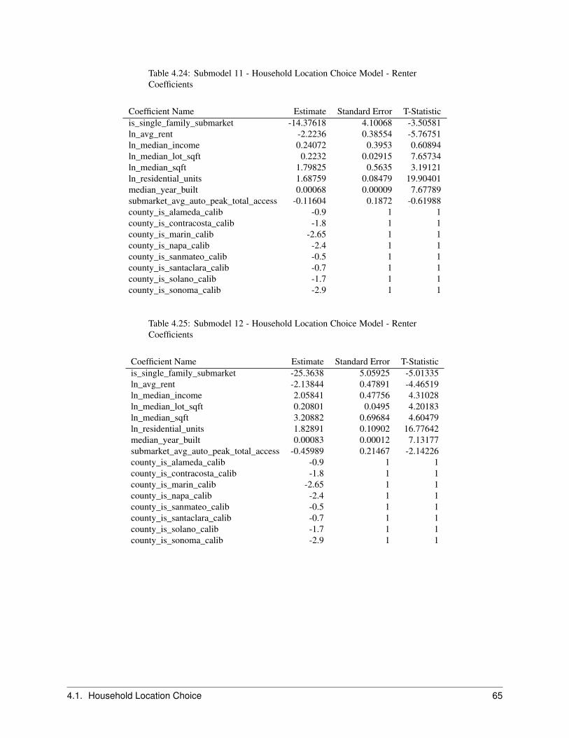
Table 4.24: Submodel 11 - Household Location Choice Model - RenterCoefficients
Coefficient Name Estimate Standard Error T-Statisticis_single_family_submarket -14.37618 4.10068 -3.50581ln_avg_rent -2.2236 0.38554 -5.76751ln_median_income 0.24072 0.3953 0.60894ln_median_lot_sqft 0.2232 0.02915 7.65734ln_median_sqft 1.79825 0.5635 3.19121ln_residential_units 1.68759 0.08479 19.90401median_year_built 0.00068 0.00009 7.67789submarket_avg_auto_peak_total_access -0.11604 0.1872 -0.61988county_is_alameda_calib -0.9 1 1county_is_contracosta_calib -1.8 1 1county_is_marin_calib -2.65 1 1county_is_napa_calib -2.4 1 1county_is_sanmateo_calib -0.5 1 1county_is_santaclara_calib -0.7 1 1county_is_solano_calib -1.7 1 1county_is_sonoma_calib -2.9 1 1
Table 4.25: Submodel 12 - Household Location Choice Model - RenterCoefficients
Coefficient Name Estimate Standard Error T-Statisticis_single_family_submarket -25.3638 5.05925 -5.01335ln_avg_rent -2.13844 0.47891 -4.46519ln_median_income 2.05841 0.47756 4.31028ln_median_lot_sqft 0.20801 0.0495 4.20183ln_median_sqft 3.20882 0.69684 4.60479ln_residential_units 1.82891 0.10902 16.77642median_year_built 0.00083 0.00012 7.13177submarket_avg_auto_peak_total_access -0.45989 0.21467 -2.14226county_is_alameda_calib -0.9 1 1county_is_contracosta_calib -1.8 1 1county_is_marin_calib -2.65 1 1county_is_napa_calib -2.4 1 1county_is_sanmateo_calib -0.5 1 1county_is_santaclara_calib -0.7 1 1county_is_solano_calib -1.7 1 1county_is_sonoma_calib -2.9 1 1
4.1. Household Location Choice 65

4.2 Business Location Choice
In the Business Location Choice Model (BLCM), we predict the probability that an establishment that is either new(from the Business Transition model), or has moved within the region (Business Relocation model), will be located ata particular employment submarket location. Employment submarkets are defined as jurisdiction, building type, andtransit-proximity combinations.
The BLCM is specified as a multinomial logit (MNL) model, with separate equations estimated for each employmentsector. An MNL is applied to estimate the probability that each establishment will move to each of the alternativeemployment submarkets under consideration. Monte Carlo simulation is used to generate a decision to locate ina particular employment submarket. Once this choice is made, the establishment is assigned to the employmentsubmarket. In the next step, establishments are assigned to specific parcel-level buildings within the employmentsubmarket using a simple location choice model that accounts for available job spaces within buildings. BusinessLocation Choice Model coefficients are presented in Table 4.26.
The number of job spots available in an employment submarket that establishments can locate in will depend mainlyon the total square footage of non-residential floorspace in the employment submarket, and on the square feet peremployee in the building type that the employment submarket represents (for each building type, a certain number ofsquare feet are defined as the minimum to support each job).
BLCM estimation has been performed for all sectors except government. In the base-year, existing establishmentswere assigned to buildings. The BLCM is comprised of a number of submodels, one for each modeled employmentsector. In simulation, the BLCM is run after the Business Transition and Business Relocation models. Establishmentchoice of employment submarket is simulated by submodel, and once all establishments have selected an employmentsubmarket with capacity, they are allocated to specific buildings with capacity within the employment submarket.Each submodel was specified independently. The variable sets were somewhat similar across submodels althoughthere is quite a bit of variation owing to the principal that establishments in different sectors predicate their locationchoices on different factors. It is hypothesized that establishment choice of location is positively associated withaccessibility, negatively associated with price, and positively associated with non-residential square footage. Forcertain employment sector submodels, a positive association with transit-presence and jobs of the same sector ishypothesized. The relationship between establishments and buildings of a certain type (such as office structures), andbetween establishments and population, is hypothesized to vary by employment sector.
66 Chapter 4. Model Estimation for the Bay Area
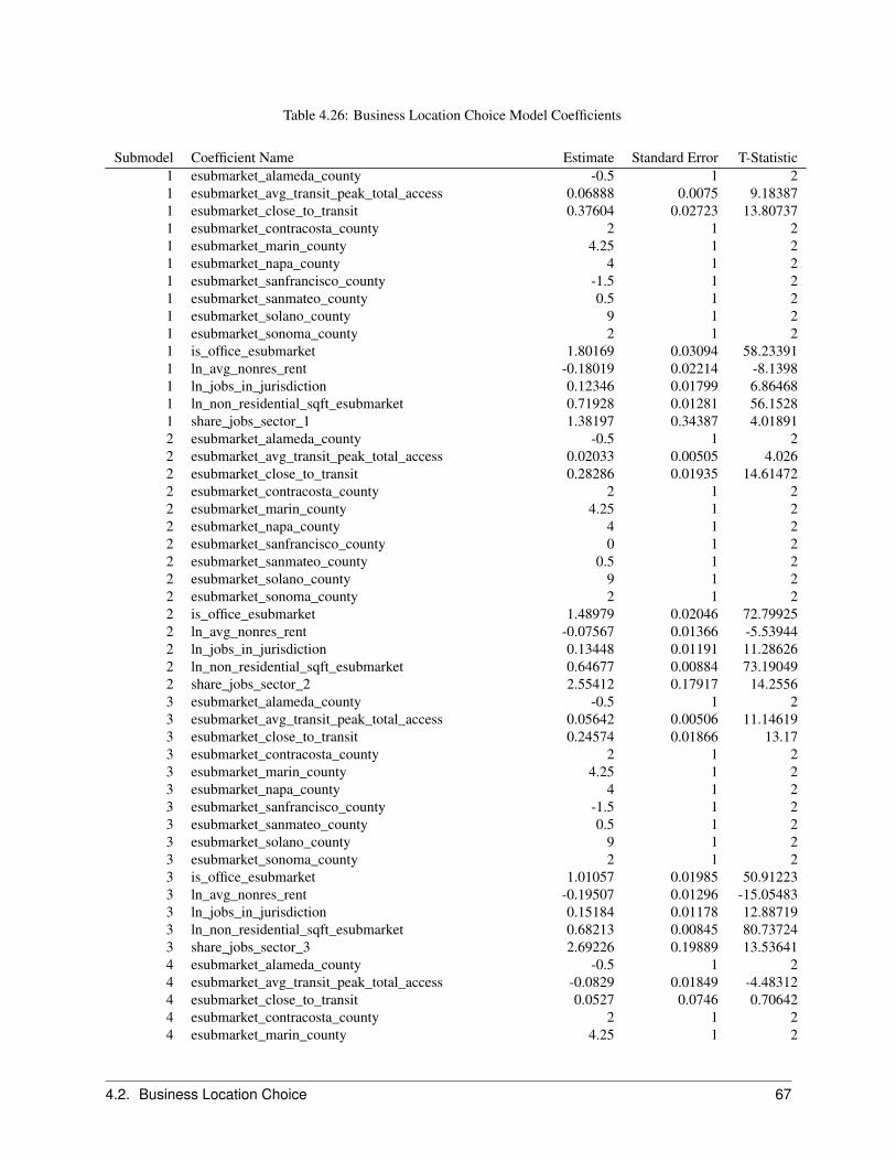
Table 4.26: Business Location Choice Model Coefficients
Submodel Coefficient Name Estimate Standard Error T-Statistic1 esubmarket_alameda_county -0.5 1 21 esubmarket_avg_transit_peak_total_access 0.06888 0.0075 9.183871 esubmarket_close_to_transit 0.37604 0.02723 13.807371 esubmarket_contracosta_county 2 1 21 esubmarket_marin_county 4.25 1 21 esubmarket_napa_county 4 1 21 esubmarket_sanfrancisco_county -1.5 1 21 esubmarket_sanmateo_county 0.5 1 21 esubmarket_solano_county 9 1 21 esubmarket_sonoma_county 2 1 21 is_office_esubmarket 1.80169 0.03094 58.233911 ln_avg_nonres_rent -0.18019 0.02214 -8.13981 ln_jobs_in_jurisdiction 0.12346 0.01799 6.864681 ln_non_residential_sqft_esubmarket 0.71928 0.01281 56.15281 share_jobs_sector_1 1.38197 0.34387 4.018912 esubmarket_alameda_county -0.5 1 22 esubmarket_avg_transit_peak_total_access 0.02033 0.00505 4.0262 esubmarket_close_to_transit 0.28286 0.01935 14.614722 esubmarket_contracosta_county 2 1 22 esubmarket_marin_county 4.25 1 22 esubmarket_napa_county 4 1 22 esubmarket_sanfrancisco_county 0 1 22 esubmarket_sanmateo_county 0.5 1 22 esubmarket_solano_county 9 1 22 esubmarket_sonoma_county 2 1 22 is_office_esubmarket 1.48979 0.02046 72.799252 ln_avg_nonres_rent -0.07567 0.01366 -5.539442 ln_jobs_in_jurisdiction 0.13448 0.01191 11.286262 ln_non_residential_sqft_esubmarket 0.64677 0.00884 73.190492 share_jobs_sector_2 2.55412 0.17917 14.25563 esubmarket_alameda_county -0.5 1 23 esubmarket_avg_transit_peak_total_access 0.05642 0.00506 11.146193 esubmarket_close_to_transit 0.24574 0.01866 13.173 esubmarket_contracosta_county 2 1 23 esubmarket_marin_county 4.25 1 23 esubmarket_napa_county 4 1 23 esubmarket_sanfrancisco_county -1.5 1 23 esubmarket_sanmateo_county 0.5 1 23 esubmarket_solano_county 9 1 23 esubmarket_sonoma_county 2 1 23 is_office_esubmarket 1.01057 0.01985 50.912233 ln_avg_nonres_rent -0.19507 0.01296 -15.054833 ln_jobs_in_jurisdiction 0.15184 0.01178 12.887193 ln_non_residential_sqft_esubmarket 0.68213 0.00845 80.737243 share_jobs_sector_3 2.69226 0.19889 13.536414 esubmarket_alameda_county -0.5 1 24 esubmarket_avg_transit_peak_total_access -0.0829 0.01849 -4.483124 esubmarket_close_to_transit 0.0527 0.0746 0.706424 esubmarket_contracosta_county 2 1 24 esubmarket_marin_county 4.25 1 2
4.2. Business Location Choice 67
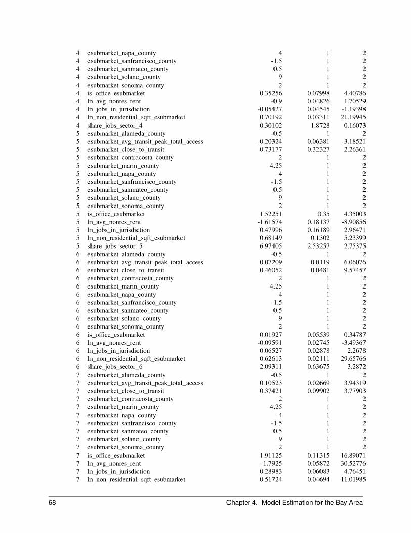
4 esubmarket_napa_county 4 1 24 esubmarket_sanfrancisco_county -1.5 1 24 esubmarket_sanmateo_county 0.5 1 24 esubmarket_solano_county 9 1 24 esubmarket_sonoma_county 2 1 24 is_office_esubmarket 0.35256 0.07998 4.407864 ln_avg_nonres_rent -0.9 0.04826 1.705294 ln_jobs_in_jurisdiction -0.05427 0.04545 -1.193984 ln_non_residential_sqft_esubmarket 0.70192 0.03311 21.199454 share_jobs_sector_4 0.30102 1.8728 0.160735 esubmarket_alameda_county -0.5 1 25 esubmarket_avg_transit_peak_total_access -0.20324 0.06381 -3.185215 esubmarket_close_to_transit 0.73177 0.32327 2.263615 esubmarket_contracosta_county 2 1 25 esubmarket_marin_county 4.25 1 25 esubmarket_napa_county 4 1 25 esubmarket_sanfrancisco_county -1.5 1 25 esubmarket_sanmateo_county 0.5 1 25 esubmarket_solano_county 9 1 25 esubmarket_sonoma_county 2 1 25 is_office_esubmarket 1.52251 0.35 4.350035 ln_avg_nonres_rent -1.61574 0.18137 -8.908565 ln_jobs_in_jurisdiction 0.47996 0.16189 2.964715 ln_non_residential_sqft_esubmarket 0.68149 0.1302 5.233995 share_jobs_sector_5 6.97405 2.53257 2.753756 esubmarket_alameda_county -0.5 1 26 esubmarket_avg_transit_peak_total_access 0.07209 0.0119 6.060766 esubmarket_close_to_transit 0.46052 0.0481 9.574576 esubmarket_contracosta_county 2 1 26 esubmarket_marin_county 4.25 1 26 esubmarket_napa_county 4 1 26 esubmarket_sanfrancisco_county -1.5 1 26 esubmarket_sanmateo_county 0.5 1 26 esubmarket_solano_county 9 1 26 esubmarket_sonoma_county 2 1 26 is_office_esubmarket 0.01927 0.05539 0.347876 ln_avg_nonres_rent -0.09591 0.02745 -3.493676 ln_jobs_in_jurisdiction 0.06527 0.02878 2.26786 ln_non_residential_sqft_esubmarket 0.62613 0.02111 29.657666 share_jobs_sector_6 2.09311 0.63675 3.28727 esubmarket_alameda_county -0.5 1 27 esubmarket_avg_transit_peak_total_access 0.10523 0.02669 3.943197 esubmarket_close_to_transit 0.37421 0.09902 3.779037 esubmarket_contracosta_county 2 1 27 esubmarket_marin_county 4.25 1 27 esubmarket_napa_county 4 1 27 esubmarket_sanfrancisco_county -1.5 1 27 esubmarket_sanmateo_county 0.5 1 27 esubmarket_solano_county 9 1 27 esubmarket_sonoma_county 2 1 27 is_office_esubmarket 1.91125 0.11315 16.890717 ln_avg_nonres_rent -1.7925 0.05872 -30.527767 ln_jobs_in_jurisdiction 0.28983 0.06083 4.764517 ln_non_residential_sqft_esubmarket 0.51724 0.04694 11.01985
68 Chapter 4. Model Estimation for the Bay Area

7 share_jobs_sector_7 5.78703 0.64838 8.925298 esubmarket_alameda_county -0.5 1 28 esubmarket_avg_transit_peak_total_access 0.1258 0.02088 6.025548 esubmarket_close_to_transit 0.1935 0.0788 2.455458 esubmarket_contracosta_county 2 1 28 esubmarket_marin_county 4.25 1 28 esubmarket_napa_county 4 1 28 esubmarket_sanfrancisco_county -1.5 1 28 esubmarket_sanmateo_county 0.5 1 28 esubmarket_solano_county 9 1 28 esubmarket_sonoma_county 2 1 28 is_office_esubmarket 1.18873 0.08112 14.65478 ln_avg_nonres_rent -0.66606 0.04804 -13.864218 ln_jobs_in_jurisdiction 0.09967 0.04983 2.000458 ln_non_residential_sqft_esubmarket 0.61618 0.03553 17.344658 share_jobs_sector_8 1.05183 5.52571 0.190359 esubmarket_alameda_county -0.5 1 29 esubmarket_avg_transit_peak_total_access 0.06197 0.00783 7.913739 esubmarket_close_to_transit 0.41182 0.03014 13.661599 esubmarket_contracosta_county 2 1 29 esubmarket_marin_county 4.25 1 29 esubmarket_napa_county 4 1 29 esubmarket_sanfrancisco_county -1.5 1 29 esubmarket_sanmateo_county 0.5 1 29 esubmarket_solano_county 9 1 29 esubmarket_sonoma_county 2 1 29 is_office_esubmarket -0.69203 0.04007 -17.268479 ln_avg_nonres_rent -0.9 0.01713 4.205679 ln_jobs_in_jurisdiction 0.09057 0.01892 4.786029 ln_non_residential_sqft_esubmarket 0.65221 0.01347 48.427259 share_jobs_sector_9 1.97623 0.38107 5.18599
10 esubmarket_alameda_county -0.5 1 210 esubmarket_avg_transit_peak_total_access 0.07304 0.0086 8.4924610 esubmarket_close_to_transit 0.48235 0.03221 14.9755210 esubmarket_contracosta_county 2 1 210 esubmarket_marin_county 4.25 1 210 esubmarket_napa_county 4 1 210 esubmarket_sanfrancisco_county -1.5 1 210 esubmarket_sanmateo_county 0.5 1 210 esubmarket_solano_county 9 1 210 esubmarket_sonoma_county 2 1 210 is_office_esubmarket -1.29264 0.04638 -27.8687810 ln_avg_nonres_rent -0.9 0.01892 37.1743810 ln_jobs_in_jurisdiction -0.02215 0.02239 -0.9892610 ln_non_residential_sqft_esubmarket 0.74465 0.01473 50.5618310 share_jobs_sector_10 1.92532 0.43434 4.4327411 esubmarket_alameda_county -0.5 1 211 esubmarket_avg_transit_peak_total_access 0.00678 0.0064 1.0591711 esubmarket_close_to_transit 0.11513 0.02473 4.6547411 esubmarket_contracosta_county 2 1 211 esubmarket_marin_county 4.25 1 211 esubmarket_napa_county 4 1 211 esubmarket_sanfrancisco_county -1.5 1 211 esubmarket_sanmateo_county 0.5 1 2
4.2. Business Location Choice 69
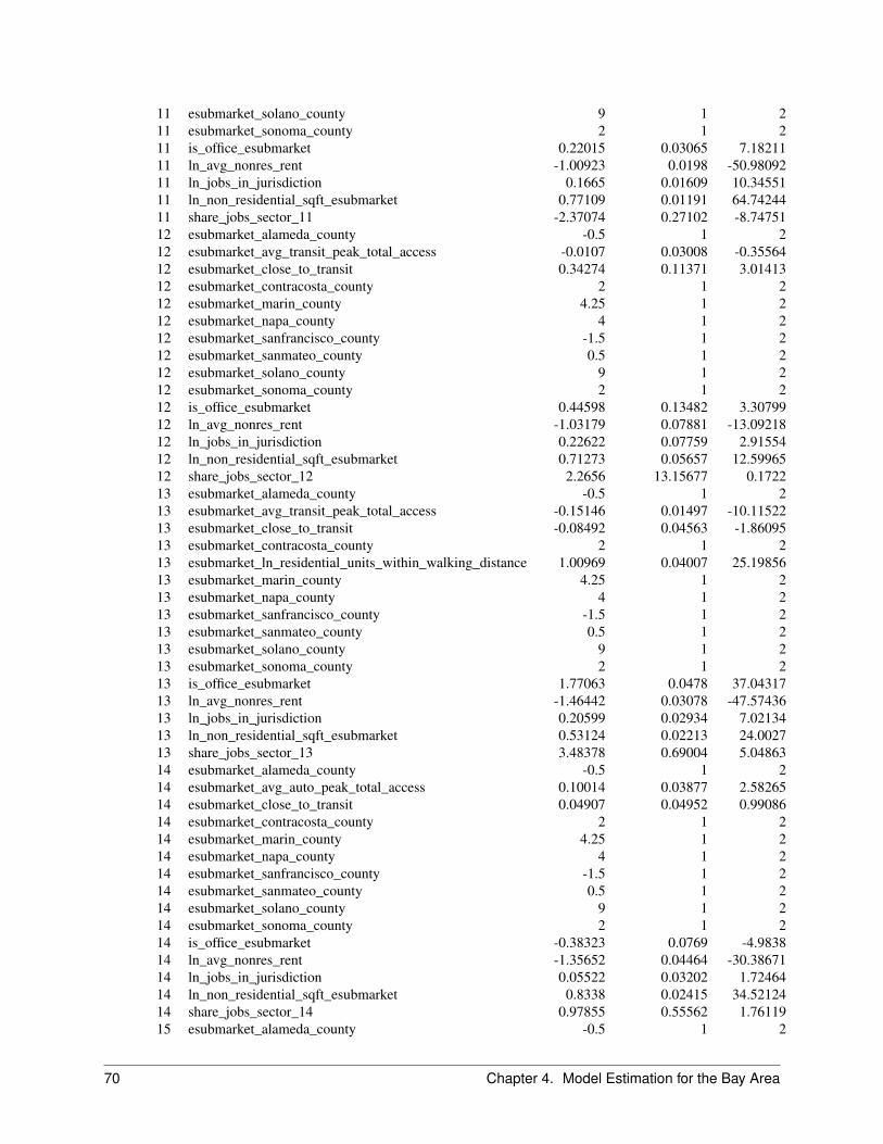
11 esubmarket_solano_county 9 1 211 esubmarket_sonoma_county 2 1 211 is_office_esubmarket 0.22015 0.03065 7.1821111 ln_avg_nonres_rent -1.00923 0.0198 -50.9809211 ln_jobs_in_jurisdiction 0.1665 0.01609 10.3455111 ln_non_residential_sqft_esubmarket 0.77109 0.01191 64.7424411 share_jobs_sector_11 -2.37074 0.27102 -8.7475112 esubmarket_alameda_county -0.5 1 212 esubmarket_avg_transit_peak_total_access -0.0107 0.03008 -0.3556412 esubmarket_close_to_transit 0.34274 0.11371 3.0141312 esubmarket_contracosta_county 2 1 212 esubmarket_marin_county 4.25 1 212 esubmarket_napa_county 4 1 212 esubmarket_sanfrancisco_county -1.5 1 212 esubmarket_sanmateo_county 0.5 1 212 esubmarket_solano_county 9 1 212 esubmarket_sonoma_county 2 1 212 is_office_esubmarket 0.44598 0.13482 3.3079912 ln_avg_nonres_rent -1.03179 0.07881 -13.0921812 ln_jobs_in_jurisdiction 0.22622 0.07759 2.9155412 ln_non_residential_sqft_esubmarket 0.71273 0.05657 12.5996512 share_jobs_sector_12 2.2656 13.15677 0.172213 esubmarket_alameda_county -0.5 1 213 esubmarket_avg_transit_peak_total_access -0.15146 0.01497 -10.1152213 esubmarket_close_to_transit -0.08492 0.04563 -1.8609513 esubmarket_contracosta_county 2 1 213 esubmarket_ln_residential_units_within_walking_distance 1.00969 0.04007 25.1985613 esubmarket_marin_county 4.25 1 213 esubmarket_napa_county 4 1 213 esubmarket_sanfrancisco_county -1.5 1 213 esubmarket_sanmateo_county 0.5 1 213 esubmarket_solano_county 9 1 213 esubmarket_sonoma_county 2 1 213 is_office_esubmarket 1.77063 0.0478 37.0431713 ln_avg_nonres_rent -1.46442 0.03078 -47.5743613 ln_jobs_in_jurisdiction 0.20599 0.02934 7.0213413 ln_non_residential_sqft_esubmarket 0.53124 0.02213 24.002713 share_jobs_sector_13 3.48378 0.69004 5.0486314 esubmarket_alameda_county -0.5 1 214 esubmarket_avg_auto_peak_total_access 0.10014 0.03877 2.5826514 esubmarket_close_to_transit 0.04907 0.04952 0.9908614 esubmarket_contracosta_county 2 1 214 esubmarket_marin_county 4.25 1 214 esubmarket_napa_county 4 1 214 esubmarket_sanfrancisco_county -1.5 1 214 esubmarket_sanmateo_county 0.5 1 214 esubmarket_solano_county 9 1 214 esubmarket_sonoma_county 2 1 214 is_office_esubmarket -0.38323 0.0769 -4.983814 ln_avg_nonres_rent -1.35652 0.04464 -30.3867114 ln_jobs_in_jurisdiction 0.05522 0.03202 1.7246414 ln_non_residential_sqft_esubmarket 0.8338 0.02415 34.5212414 share_jobs_sector_14 0.97855 0.55562 1.7611915 esubmarket_alameda_county -0.5 1 2
70 Chapter 4. Model Estimation for the Bay Area
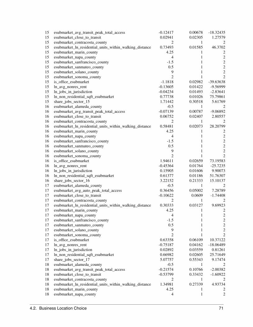
15 esubmarket_avg_transit_peak_total_access -0.12417 0.00678 -18.3243515 esubmarket_close_to_transit 0.02941 0.02305 1.2757915 esubmarket_contracosta_county 2 1 215 esubmarket_ln_residential_units_within_walking_distance 0.73493 0.01585 46.370215 esubmarket_marin_county 4.25 1 215 esubmarket_napa_county 4 1 215 esubmarket_sanfrancisco_county -1.5 1 215 esubmarket_sanmateo_county 0.5 1 215 esubmarket_solano_county 9 1 215 esubmarket_sonoma_county 2 1 215 is_office_esubmarket -1.1818 0.02982 -39.6363815 ln_avg_nonres_rent -0.13605 0.01422 -9.5699915 ln_jobs_in_jurisdiction -0.04234 0.01493 -2.8364115 ln_non_residential_sqft_esubmarket 0.77738 0.01026 75.7986115 share_jobs_sector_15 1.71442 0.30518 5.6176916 esubmarket_alameda_county -0.5 1 216 esubmarket_avg_transit_peak_total_access -0.07139 0.00787 -9.0689216 esubmarket_close_to_transit 0.06752 0.02407 2.8055716 esubmarket_contracosta_county 2 1 216 esubmarket_ln_residential_units_within_walking_distance 0.58481 0.02073 28.2079916 esubmarket_marin_county 4.25 1 216 esubmarket_napa_county 4 1 216 esubmarket_sanfrancisco_county -1.5 1 216 esubmarket_sanmateo_county 0.5 1 216 esubmarket_solano_county 9 1 216 esubmarket_sonoma_county 2 1 216 is_office_esubmarket 1.94611 0.02659 73.1958316 ln_avg_nonres_rent -0.45364 0.01764 -25.723516 ln_jobs_in_jurisdiction 0.15905 0.01606 9.9007316 ln_non_residential_sqft_esubmarket 0.61377 0.01186 51.7630716 share_jobs_sector_16 3.22152 0.21333 15.1013717 esubmarket_alameda_county -0.5 1 217 esubmarket_avg_auto_peak_total_access 0.36456 0.05002 7.2878917 esubmarket_close_to_transit -0.10622 0.0609 -1.7440817 esubmarket_contracosta_county 2 1 217 esubmarket_ln_residential_units_within_walking_distance 0.30333 0.03127 9.6992317 esubmarket_marin_county 4.25 1 217 esubmarket_napa_county 4 1 217 esubmarket_sanfrancisco_county -1.5 1 217 esubmarket_sanmateo_county 0.5 1 217 esubmarket_solano_county 9 1 217 esubmarket_sonoma_county 2 1 217 is_office_esubmarket 0.63358 0.06109 10.3712217 ln_avg_nonres_rent -0.75187 0.04162 -18.0648917 ln_jobs_in_jurisdiction 0.02892 0.03559 0.8126117 ln_non_residential_sqft_esubmarket 0.66982 0.02605 25.7164917 share_jobs_sector_17 5.07757 0.55343 9.1747418 esubmarket_alameda_county -0.5 1 218 esubmarket_avg_transit_peak_total_access -0.21574 0.10766 -2.0038218 esubmarket_close_to_transit -0.53799 0.33432 -1.6092218 esubmarket_contracosta_county 2 1 218 esubmarket_ln_residential_units_within_walking_distance 1.34981 0.27339 4.9373418 esubmarket_marin_county 4.25 1 218 esubmarket_napa_county 4 1 2
4.2. Business Location Choice 71

18 esubmarket_sanfrancisco_county -1.5 1 218 esubmarket_sanmateo_county 0.5 1 218 esubmarket_solano_county 9 1 218 esubmarket_sonoma_county 2 1 218 is_office_esubmarket 1.59352 0.27912 5.7090318 ln_avg_nonres_rent -2.27596 0.21961 -10.3637118 ln_jobs_in_jurisdiction 0.61951 0.18557 3.3384118 ln_non_residential_sqft_esubmarket 0.56889 0.15253 3.7296718 share_jobs_sector_18 11.38959 1.82986 6.2242919 esubmarket_alameda_county -0.5 1 219 esubmarket_avg_auto_peak_total_access -0.18859 0.10039 -1.8785719 esubmarket_close_to_transit 0.14666 0.12413 1.1815319 esubmarket_contracosta_county 2 1 219 esubmarket_ln_residential_units_within_walking_distance 0.31742 0.06911 4.5929519 esubmarket_marin_county 4.25 1 219 esubmarket_napa_county 4 1 219 esubmarket_sanfrancisco_county -1.5 1 219 esubmarket_sanmateo_county 0.5 1 219 esubmarket_solano_county 9 1 219 esubmarket_sonoma_county 2 1 219 is_office_esubmarket 1.03137 0.12546 8.2208819 ln_avg_nonres_rent -1.68234 0.09375 -17.9445319 ln_jobs_in_jurisdiction 0.23593 0.07482 3.1532619 ln_non_residential_sqft_esubmarket 0.72809 0.05324 13.6765419 share_jobs_sector_19 2.39901 6.84219 0.3506220 esubmarket_alameda_county -0.5 1 220 esubmarket_avg_auto_peak_total_access -0.02755 0.02656 -1.0372220 esubmarket_close_to_transit -0.1013 0.0335 -3.0236220 esubmarket_contracosta_county 2 1 220 esubmarket_ln_residential_units_within_walking_distance 0.25967 0.01839 14.1236520 esubmarket_marin_county 4.25 1 220 esubmarket_napa_county 4 1 220 esubmarket_sanfrancisco_county -1.5 1 220 esubmarket_sanmateo_county 0.5 1 220 esubmarket_solano_county 9 1 220 esubmarket_sonoma_county 2 1 220 is_office_esubmarket 0.33675 0.03797 8.8686620 ln_avg_nonres_rent -1.1891 0.02414 -49.2612820 ln_jobs_in_jurisdiction 0.11749 0.01934 6.0760320 ln_non_residential_sqft_esubmarket 0.65141 0.01474 44.1903720 share_jobs_sector_20 3.10188 0.38667 8.0219321 esubmarket_alameda_county -0.5 1 221 esubmarket_avg_transit_peak_total_access -0.12336 0.06334 -1.9474821 esubmarket_close_to_transit -0.56687 0.21655 -2.6177821 esubmarket_contracosta_county 2 1 221 esubmarket_ln_residential_units_within_walking_distance 0.00029 0.12876 0.0022521 esubmarket_marin_county 4.25 1 221 esubmarket_napa_county 4 1 221 esubmarket_sanfrancisco_county -1.5 1 221 esubmarket_sanmateo_county 0.5 1 221 esubmarket_solano_county 9 1 221 esubmarket_sonoma_county 2 1 221 is_office_esubmarket 0.54696 0.23634 2.3143521 ln_avg_nonres_rent -0.2334 0.17513 -1.33271
72 Chapter 4. Model Estimation for the Bay Area
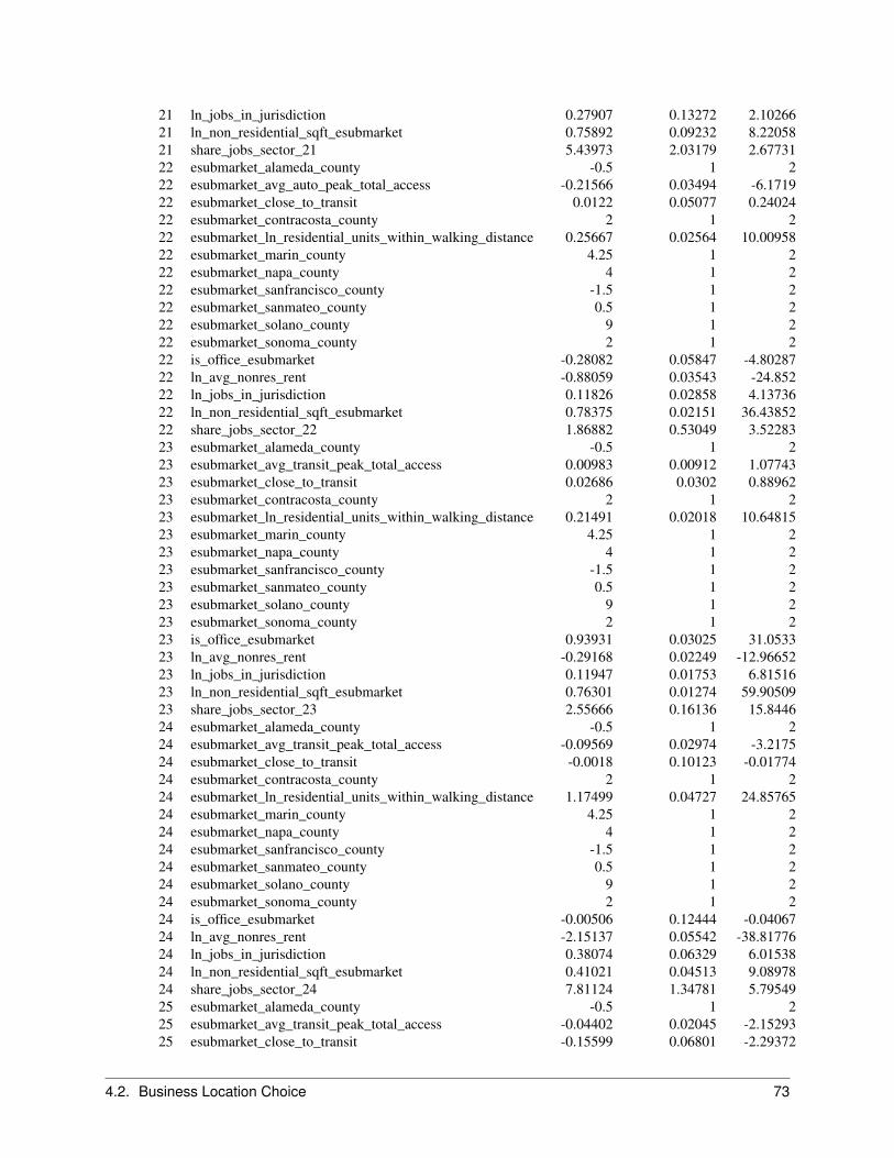
21 ln_jobs_in_jurisdiction 0.27907 0.13272 2.1026621 ln_non_residential_sqft_esubmarket 0.75892 0.09232 8.2205821 share_jobs_sector_21 5.43973 2.03179 2.6773122 esubmarket_alameda_county -0.5 1 222 esubmarket_avg_auto_peak_total_access -0.21566 0.03494 -6.171922 esubmarket_close_to_transit 0.0122 0.05077 0.2402422 esubmarket_contracosta_county 2 1 222 esubmarket_ln_residential_units_within_walking_distance 0.25667 0.02564 10.0095822 esubmarket_marin_county 4.25 1 222 esubmarket_napa_county 4 1 222 esubmarket_sanfrancisco_county -1.5 1 222 esubmarket_sanmateo_county 0.5 1 222 esubmarket_solano_county 9 1 222 esubmarket_sonoma_county 2 1 222 is_office_esubmarket -0.28082 0.05847 -4.8028722 ln_avg_nonres_rent -0.88059 0.03543 -24.85222 ln_jobs_in_jurisdiction 0.11826 0.02858 4.1373622 ln_non_residential_sqft_esubmarket 0.78375 0.02151 36.4385222 share_jobs_sector_22 1.86882 0.53049 3.5228323 esubmarket_alameda_county -0.5 1 223 esubmarket_avg_transit_peak_total_access 0.00983 0.00912 1.0774323 esubmarket_close_to_transit 0.02686 0.0302 0.8896223 esubmarket_contracosta_county 2 1 223 esubmarket_ln_residential_units_within_walking_distance 0.21491 0.02018 10.6481523 esubmarket_marin_county 4.25 1 223 esubmarket_napa_county 4 1 223 esubmarket_sanfrancisco_county -1.5 1 223 esubmarket_sanmateo_county 0.5 1 223 esubmarket_solano_county 9 1 223 esubmarket_sonoma_county 2 1 223 is_office_esubmarket 0.93931 0.03025 31.053323 ln_avg_nonres_rent -0.29168 0.02249 -12.9665223 ln_jobs_in_jurisdiction 0.11947 0.01753 6.8151623 ln_non_residential_sqft_esubmarket 0.76301 0.01274 59.9050923 share_jobs_sector_23 2.55666 0.16136 15.844624 esubmarket_alameda_county -0.5 1 224 esubmarket_avg_transit_peak_total_access -0.09569 0.02974 -3.217524 esubmarket_close_to_transit -0.0018 0.10123 -0.0177424 esubmarket_contracosta_county 2 1 224 esubmarket_ln_residential_units_within_walking_distance 1.17499 0.04727 24.8576524 esubmarket_marin_county 4.25 1 224 esubmarket_napa_county 4 1 224 esubmarket_sanfrancisco_county -1.5 1 224 esubmarket_sanmateo_county 0.5 1 224 esubmarket_solano_county 9 1 224 esubmarket_sonoma_county 2 1 224 is_office_esubmarket -0.00506 0.12444 -0.0406724 ln_avg_nonres_rent -2.15137 0.05542 -38.8177624 ln_jobs_in_jurisdiction 0.38074 0.06329 6.0153824 ln_non_residential_sqft_esubmarket 0.41021 0.04513 9.0897824 share_jobs_sector_24 7.81124 1.34781 5.7954925 esubmarket_alameda_county -0.5 1 225 esubmarket_avg_transit_peak_total_access -0.04402 0.02045 -2.1529325 esubmarket_close_to_transit -0.15599 0.06801 -2.29372
4.2. Business Location Choice 73
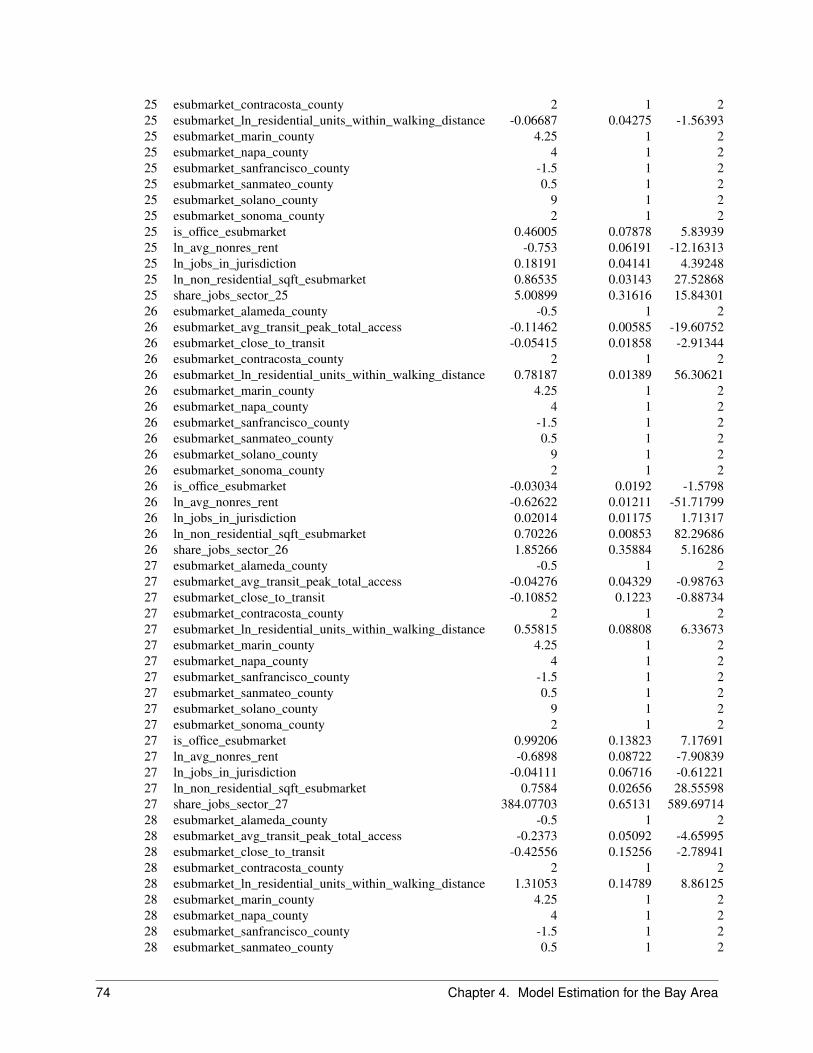
25 esubmarket_contracosta_county 2 1 225 esubmarket_ln_residential_units_within_walking_distance -0.06687 0.04275 -1.5639325 esubmarket_marin_county 4.25 1 225 esubmarket_napa_county 4 1 225 esubmarket_sanfrancisco_county -1.5 1 225 esubmarket_sanmateo_county 0.5 1 225 esubmarket_solano_county 9 1 225 esubmarket_sonoma_county 2 1 225 is_office_esubmarket 0.46005 0.07878 5.8393925 ln_avg_nonres_rent -0.753 0.06191 -12.1631325 ln_jobs_in_jurisdiction 0.18191 0.04141 4.3924825 ln_non_residential_sqft_esubmarket 0.86535 0.03143 27.5286825 share_jobs_sector_25 5.00899 0.31616 15.8430126 esubmarket_alameda_county -0.5 1 226 esubmarket_avg_transit_peak_total_access -0.11462 0.00585 -19.6075226 esubmarket_close_to_transit -0.05415 0.01858 -2.9134426 esubmarket_contracosta_county 2 1 226 esubmarket_ln_residential_units_within_walking_distance 0.78187 0.01389 56.3062126 esubmarket_marin_county 4.25 1 226 esubmarket_napa_county 4 1 226 esubmarket_sanfrancisco_county -1.5 1 226 esubmarket_sanmateo_county 0.5 1 226 esubmarket_solano_county 9 1 226 esubmarket_sonoma_county 2 1 226 is_office_esubmarket -0.03034 0.0192 -1.579826 ln_avg_nonres_rent -0.62622 0.01211 -51.7179926 ln_jobs_in_jurisdiction 0.02014 0.01175 1.7131726 ln_non_residential_sqft_esubmarket 0.70226 0.00853 82.2968626 share_jobs_sector_26 1.85266 0.35884 5.1628627 esubmarket_alameda_county -0.5 1 227 esubmarket_avg_transit_peak_total_access -0.04276 0.04329 -0.9876327 esubmarket_close_to_transit -0.10852 0.1223 -0.8873427 esubmarket_contracosta_county 2 1 227 esubmarket_ln_residential_units_within_walking_distance 0.55815 0.08808 6.3367327 esubmarket_marin_county 4.25 1 227 esubmarket_napa_county 4 1 227 esubmarket_sanfrancisco_county -1.5 1 227 esubmarket_sanmateo_county 0.5 1 227 esubmarket_solano_county 9 1 227 esubmarket_sonoma_county 2 1 227 is_office_esubmarket 0.99206 0.13823 7.1769127 ln_avg_nonres_rent -0.6898 0.08722 -7.9083927 ln_jobs_in_jurisdiction -0.04111 0.06716 -0.6122127 ln_non_residential_sqft_esubmarket 0.7584 0.02656 28.5559827 share_jobs_sector_27 384.07703 0.65131 589.6971428 esubmarket_alameda_county -0.5 1 228 esubmarket_avg_transit_peak_total_access -0.2373 0.05092 -4.6599528 esubmarket_close_to_transit -0.42556 0.15256 -2.7894128 esubmarket_contracosta_county 2 1 228 esubmarket_ln_residential_units_within_walking_distance 1.31053 0.14789 8.8612528 esubmarket_marin_county 4.25 1 228 esubmarket_napa_county 4 1 228 esubmarket_sanfrancisco_county -1.5 1 228 esubmarket_sanmateo_county 0.5 1 2
74 Chapter 4. Model Estimation for the Bay Area

28 esubmarket_solano_county 9 1 228 esubmarket_sonoma_county 2 1 228 is_office_esubmarket 1.88894 0.15419 12.2504328 ln_avg_nonres_rent -2.75949 0.11578 -23.8347528 ln_jobs_in_jurisdiction 0.44782 0.10402 4.3051128 ln_non_residential_sqft_esubmarket 0.42823 0.07966 5.375628 share_jobs_sector_28 6.95702 2.99011 2.32668
4.2. Business Location Choice 75

4.3 Real Estate Price Model
The Real Estate Price Model (REPM) is an Ordinary Least Squares (OLS) regression model that predicts the priceof residential units and non-residential square footage. UrbanSim uses prices as the indicator of the match betweendemand and supply of various development types, and of the relative market valuations for attributes of housing,nonresidential space, and location. Since prices enter the location choice utility functions for most BLCM and HLCMsubmodels, an adjustment in prices will alter location preferences. Similarly, an adjustment in price influences theproject location decisions of developers.
Prices are modeled using a hedonic regression of unit value on attributes of the building and its environment. The unitwhose value is being modeled is either a residential unit or a non-residential square foot. For residential buildings, thedependent variable is the natural log of the price per residential unit or rent per residential unit (depending on tenure).Price per residential unit is the building improvement value divided by the total number of residential units in thebuilding. Rent per residential units is based on predicted rents based on a regression equation estimated off of Costardata. In the case of single-family detached buildings, the unit price equals the building improvement value. Separateregressions are run for each residential building type. For non-residential buildings, the dependent value is the naturallog of the rent per nonresidential square-foot. Separate regressions are run for each non-residential building type.Explanatory variables in the price models include building type dummies, accessibility, household income, number ofstories, building age (whether or not build before 1930), and residential unit square footage. Prices are hypothesizedto be positively associated with income, accessibility, stories, and square footage. Being built before 1930 (historicstructures) is also hypothesized to exhibit a positive relationship with price.
The REPM updates the unit price attributes in the building table or the residential_units table. Instead of storing priceas the natural log of price (this is what is actually estimated and predicted), the REPM automatically exponentiates thepredicted value so that the unit prices stored in the tables are more understandable. The REPM models run near thebeginning of each simulation year; prices are updated in the simulation in the following order: non-residential rent,residential rent, residential sale price. Real Estate Price Model coefficients are presented in Tables 4.27, 4.28, and 4.28.
The hedonic regression is estimated off of the the base-year buildings and residential_units tables, which areassembled from assessor records and supplemented with additional price data such as Costar. Explanatory variablesinclude measures of accessibility, real estate characteristics, proximity to amenities. The hedonic regression equationencapsulates interactions between market demand and supply, revealing an envelope of implicit valuations. Becausethe hedonic regression includes variables that are maintained as part of the simulation system, these are used to updaterelative prices during simulation. Prices are updated annually at the beginning of the simulation year and also duringan equilibration step following simulation of the demand models.
76 Chapter 4. Model Estimation for the Bay Area

Table 4.27: Non-Residential Units - Rent Model Coefficients
Coefficient Name Estimate Standard Error T-Statisticbdlg_in_san_francisco 0.11615 0.02514 4.61945bdlg_type_hotel 0.51298 0.07712 6.6514bdlg_type_mixed_use 0.73969 0.02789 26.52508bdlg_type_office 0.70843 0.01552 45.63552bdlg_type_strip_mall 0.74473 0.01701 43.76937bldg_avg_auto_peak_total_access 0.07512 0.00921 8.15595bldg_ln_average_income_within_500_meters 0.02049 0.00216 9.5065bdlg_office_x_san_francisco 1.5 1 1stories 0.01441 0.00217 6.63596constant 1.17445 0.1125 10.43933
Table 4.28: Residential Units - Sale Price Model Coefficients
Coefficient Name Estimate Standard Error T-Statisticbuilt_pre_1930 0.11892 0.00497 23.94785ln_average_income_within_500_meters 0.54556 0.00261 209.00764ln_lot_sqft 0.22366 0.00178 125.4635ln_unit_sqft 0.0106 0.00104 10.16333transit_peak_total_access 0.0081 0.00055 14.84213transit_within_half_mile 0.25349 0.01046 24.2412unit_is_single_family -0.46518 0.00581 -80.05428constant 6.32411 0.0271 233.34106
Table 4.29: Residential Units - Rent Model Coefficients
Coefficient Name Estimate Standard Error T-Statisticbuilt_pre_1930 0.05948 0.00508 11.70141ln_average_income_within_500_meters -0.00362 0.00026 -13.99987ln_unit_sqft 0.74352 0.00202 367.38391transit_peak_total_access 0.04391 0.00018 241.54031transit_within_half_mile 0.16645 0.0019 87.80073constant 2.14473 0.01382 155.19301
4.3. Real Estate Price Model 77

4.4 Calibration, Validation, and Sensitivity Analyses
This section describes calibration, validation, and sensitivity testing of the Bay Area UrbanSim model. To evaluate theempirical validity of the models, the 1-year period from 2010 to 2011 was simulated, and predictions were comparedto validation targets that assumed the continuation of recently-observed spatial patterns of growth in households,residential units, employment, and non-residential space. Sensitivity testing involved running the model out to 2040and assessing the model with respect to appropriate policy sensitivities. These exercises provide information on theforecasting capability of the models. Validation was undertaken at a number of geographic levels, but the county levelwas the focus.
Because the base-year is 2010, simulation results reflect predictions for year 2011 and beyond, for which there wasrelatively little observed data. ABAG prepared 2011 household, employment, residential unit, and built-space targetsthat were used in calibration. These targets were created based on recently observed growth and development patternsand informed by local expertise on development pressures and constraints in the Bay Area. The goal was to createtargets that reflected an extrapolation to 2011 based on normal patterns of growth during a healthy economy. A focuswas getting good measures of the inter-county distribution of growth. Creating targets based on longer, more mixedperiod was seen as valuable, since the end of the last decade included a historically sharp recession. For example,the 2011 employment targets that were calculated using 2008-2010 data implied a decline in employment for somecounties. 2011 targets calculated based on pre-recession data seemed quite a bit more reasonable to calibrate to, giventhat negative growth rates over the entire forecast period is unlikely. Calibrating to historical trends (even if only recenttrends are considered) should not be the only determining factor in a land use forecast. Fortunately, UrbanSim accountsfor a wide variety of variables that will influence growth separate from the calibration process. For example, countiesthat have historically grown very rapidly can run out of zoned capacity, shifting growth to counties that historicallyexperienced slower growth. Congestion effects and price effects can influence the spatial distribution of growth in thesimulation. These are examples of complex feedback effects that UrbanSim is designed to handle.
The 2011 household and employment targets by county were used as calibration and validation targets for the house-hold location choice model and employment location choice model. Calibration of the demand-side models consistedprimarily of adding county dummy variables to the specification and adjusting coefficient values for these dummyvariables. An iterative process of running 1-year simulations, comparing output to targets, and then adjusting countydummy coefficients to try and better match targets was the main approach to calibration of the demand-side models.Since all the models interact with each other, each result reflects the intricate interplay of multiple UrbanSim compo-nents. When adjusting one model component as part of the calibration process, results from other components wouldoften change, so an iterative and time-consuming process was needed.
The 2011 residential unit and non-residential space targets by county and building type were used as calibration andvalidation targets for the real estate developer model. Accounting for the fact that the end of the last decade wasa highly irregular and recessionary period, built space targets were prepared multiple ways- using longer periodswhere irregularities tend to average out and also using shorter fast-growth periods that reflect a healthy economy.Using faster periods of growth had the added advantage that certain rarer development types didn’t drop out of thecalibration targets. Extensive testing, adjustment, and calibration of the developer model were undertaken basedon these targets. Cost shifters (county-level factors used to shift real estate development costs up or down), priceshifters, and assumptions such as the proportion of parcels to consider for development each year were adjusted inthe calibration process. These adjustments helped move development patterns (in terms of residential units and non-residential square footage by building type) towards the pattern suggested by the targets.
The second step after validation/calibration was sensitivity testing. The model was repeatedly run out to 2040, andsimulation results were gauged with respect to their having the appropriate policy sensitivities. Runs were comparedwith respect to development outcomes, the spatial distribution of households and employment, expected differencesbetween counties, PDA-nonPDA shares, and the expected effect of policy initiatives (policies vary by scenario). Ad-justments were then made, followed by additional runs. This process of testing helped to assess reasonableness ofsimulation output and sensitivity to policies of interest, as well as providing guidance as to how to better calibrate themodel. Adjustments made as a result of the sensitivity testing included:
• Updating parcel subsidies (for scenarios where such subsidies were used to represent certain policies) based onthe simulation results to ensure that differences in development patterns between policy-based scenarios were
78 Chapter 4. Model Estimation for the Bay Area

reasonable. Differences in simulated spatial patterns between runs should reflect differences in policy contentbetween scenarios.
• Adjustments aimed to ensure that simulation results had the proper sensitivity to PDA-oriented policies. Forexample, in some scenarios we would expect more construction occurring in the PDAs due to policies that wouldmake PDAs substantially more attractive to real estate development. Simulation results should reflect this policysensitivity.
• Additional calibration to achieve a closer correspondence between simulated and target amounts of growth bycounty and PDA. 2040 growth targets from ABAG represent substantial local knowledge and expertise, so movingUrbanSim results closer to these was a desirable goal.
• Monitoring the number of unplaced households in out-years, which is a sign of simulated imbalance betweendemand and supply, and making model configuration changes to reduce the number.
Sensitivity testing facilitated the evaluation of full model results for plausibility and the extent to which expected policyeffects were seen. Where appropriate policy sensitivities were not present, model adjustments were made, followedby additional test runs. This exercise was a useful exploration of the model’s responsiveness and provided informationon the trade-offs that might be involved in implementing alternative scenarios.
4.4. Calibration, Validation, and Sensitivity Analyses 79
CHAPTER
FIVE
Software Platform
5.1 The Open Platform for Urban Simulation
UrbanSim has been implemented in an open source software platform called the Open Platform for Urban Simulation(OPUS). This section provides an overview of OPUS, beginning with a quick review of its key features.
5.1.1 Graphical User Interface
A flexible, cross-platform user interface has been implemented for OPUS that organizes functionality into convenientlyaccessible tabs oriented towards the workflow of developing and using models. The data manager tab contains a databrowser and tools for a variety of data manipulations and conversion of data to and from GIS and SQL data repositoriesto the OPUS data format, geoprocessing tools in external GIS systems such as ESRI and Postgis, and data synthesistools. The model manager provides infrasructure to create new models, configure them, specify the variables to use aspredictive variables, and estimate model parameters using Ordinary Least Squares or Maximum Likelihood methods,depending on the model. The Scenario Manager provides convenient organization of model scenarios and the capacityto launch simulations and monitor them. The Results Manager manages the voluminous output of simulations andprovides means to compute and visualize indicators derived from simulation results, and to display these results inmaps, charts and tables. The GUI is data-driven from XML files, and can be readily extended by users who wish toadd tools, variables, indicators, and other functionality.
5.1.2 Python as the Base Language
One of the most important parts in the system is the choice of programming language on which to build. This languagemust allow us to build a system with the above characteristics. After considering several different languages (C/C++,C#, Java, Perl, Python, R, Ruby) we choose Python for the language in which to implement Opus. Python provides amature object-oriented language with good management of the use of memory, freeing up the memory when an objectis no longer needed (automatic garbage collection). Python has a concise and clean syntax that results in programsthat generally are 1/5 as long as comparable Java programs. In addition, Python has an extensive set of excellent open-source libraries. Many of these libraries are coded in C/C++ and are thus are very efficient. There are also severalmechanisms for ‘wrapping’ other existing packages and thus making them available to Python code.
Some of the Python libraries used by Opus as building blocks or foundational components are:
• Numpy: an open-source Python numerical library containing a wide variety of useful and fast array functions,which are used throughout Opus to provide high performance computation for large data sets. The syntax forNumpy is quite similar to other matrix processing packages used in statistics, such as R, Gauss, Matlab, Scilab,and Octave, and it provides a very simple interface to this functionality from Python. See http://numpy.scipy.org/for more details and documentation.
• Scipy: a scientific library that builds on Numpy, and adds many kinds of statistical and computational tools, such
80
as non-linear optimization, which are used in estimating the parameters for models estimated with MaximumLikelihood methods. See http://scipy.org/ for details.
• Matplotlib: a 2-dimensional plotting package that also uses Numpy. It is used in Opus to provide charting andsimple image mapping capabilities. See http://matplotlib.sourceforge.net/ for details.
• SQLAlchemy: provides a general interface from Python to a wide variety of Database Management Sys-tems (DBMS), such as MySQL, Postgres, MS SQL Server, SQLite, and others. It allows Opus to movedata between a database environment and Opus, which stores data internally in the Numpy format. Seehttp://www.sqlalchemy.org/ for details.
• PyQt4: a Python interface to the Qt4 library for Graphical User Interface (GUI) development. This has been usedto create the new Opus/UrbanSim GUI. See http://www.riverbankcomputing.co.uk/pyqt/ for details.
Python is an interpretive language, which makes it easy to do small experiments from Python’s interactive commandline. For instance, we often write a simple test of a numarray function to confirm that our understanding of thedocumentation is correct. It is much easier to try things out in Python, than in Java or C++, for instance. At the sametime, Python has excellent support for scripting and running batch jobs, since it is easy to do a lot with a few lines ofPython, and Python ‘plays well’ with many other languages.
Python’s ability to work well for quick experiments, access high-performance libraries, and script other applicationsmeans that modelers need only learn one language for these tasks. Opus extends the abstractions available in Pythonwith domain-specific abstractions useful for urban modelers, as described below.
5.1.3 Integrated Model Estimation and Application
Model application software in the land use and transportation domain has generally been written to apply a model,provided a set of inputs that include the initial data and the model coefficients. The process of generating model coef-ficients is generally handled by a separate process, generally using commercial econometric software. Unfortunately,there are many problems that this process does not assist users in addressing, or which the process may actually exac-erbate. There are several potential sources of inconsistency that can cause significant problems in operational use, andin the experience of the authors this is one of the most common sources of problems in modelling applications.
First, if estimation and application software applications are separate, model specifications must be made redundantly- once in the estimation software and once in the application software. This raises the risk of application errors, someof which may not be perceived immediately by the user. Second, separate application and estimation software requiresthat an elaborate process be created to undertake the steps of creating an estimation data set that can be used by theestimation software, again giving rise to potential for errors. Third, there are many circumstances in which modelestimation is done in an iterative fashion, due to experimentation with the model specification, updates to data, orother reasons. As a result of these concerns, a design objective for Opus is the close integration of model estimationand application, and the use of a single repository for model specifications. This is addressed in the Opus design bydesignating a single repository for model specification, by incorporating parameter estimation as an explicit step inimplementing a model, and by providing well-integrated packages to estimate model parameters.
5.1.4 Database Management, GIS and Visualization
The extensive use of spatial data as the common element within and between models, and the need for spatial com-putations and visualization, make clear that the Opus platform requires access to these functions. Some of theseare handled internally by efficient array processing and image processing capabilities of the Python Numeric library.But database management and GIS functionality will be accessed by coupling with existing Open Source databaseservers such as MySQL (www.mysql.org) and Postgres (www.postgresql.org), and GIS libraries such as QuantumGIS(www.qgis.org). Interfaces to some commercial DBMS are available through the SQLAlchemy library. An interfaceto the ESRI ArcGIS system has been implemented and is being refined.
5.1. The Open Platform for Urban Simulation 81
5.1.5 Documentation, Examples and Tests
Documentation, examples and tests are three important ways to help users understand what a package can do, andhow to use the package. Documentation for Opus and UrbanSim is created in both Adobe portable document format(pdf) and web-based format (html, xml), and is available locally with an installation, or can be accessed at any timefrom the UrbanSim web site. The pdf format makes it easy to print the document, and can produce more readabledocuments. Web-based documentation can be easier to navigate, and are particularly useful for automatically extractedcode documentation.
5.1.6 Open Source License
The choice of a license is an crucial one for any software project, as it dictates the legal framework for the manage-ment of intellectual property embedded in the code. Opus has been released under the GNU General Public License(GPL). GPL is a standard license used for Open Source software. It allows users to obtain the source code as wellas executables, to make modifications as desired, and to redistribute the original or modified code, provided that thedistributed code also carries the same license as the original. It is a license that is intended to protect software frombeing converted to a proprietary license that would make the source code unavailable to users and developers.
5.1.7 Test, Build and Release Processes
Any software project involving more than one developer requires some infrastructure to coordinate development ac-tivities, and infrastructure is needed to test software in order to reduce the likelihood of software bugs, and a releaseprocess is needed to manage the packaging of the system for access by users. For each module written in Opus, unittests are written that validate the functioning of the module. A testing program has also been implemented that runsall the tests in all the modules within Opus as a single batch process. For the initial release process, a testing programis being used to involve a small number of developers and users in testing the code and documentation.
The release process involves three types of releases of the software: major, minor, and maintenance. The versionnumbers reflect the release status as follows: a release numbered 4.2.8 would reflect major release 4, minor release 2and maintenance release 8. Maintenance releases are for fixing bugs only. Minor releases are for modest additions offeatures, and major releases are obviously for more major changes in the system.
The Opus project currently uses the Subversion version control system for maintaining a shared repository for thecode as it is developed by multiple developers. Write access to the repository is maintained by a core group ofdevelopers who control the quality of the code in the system, and this group can evolve over time as others beginactively participating in the further development of the system. A repository will also be set up for users who wish tocontribute packages for use in Opus, with write access.
5.2 Introduction to the Graphical User Interface
This section of the documentation provides a tutorial approach to using the Graphical Interface (GUI) that has beenadded to the OPUS system. This represents a substantial initiative to make UrbanSim and OPUS more user-friendlyand accessible to modelers and model users — by reducing the need for programming expertise to use the systemeffectively to build, estimate, and use model systems for a range of applications. We think the GUI offers a substantialadvance in usability, and look forward to user feedback, and contributions from collaborators, to continue building onthis foundation.
Before starting the tutorial, please install Opus and UrbanSim on your machine if you haven’t already.
The GUI is cross-platform compatible, and has been developed using the open source Qt4 library and the PyQt Pythoninterface to it. Screenshots included in this section will be taken from all three platforms, to give a sense of the lookand feel of the GUI on each platform. After launching the GUI from any of these platforms, the main Opus GUIwindow should be displayed as in Figure 5.1 or 5.2.
82 Chapter 5. Software Platform
The organization of the GUI is based on an expectation that the work flow for developing and using models can be ef-fectively organized into tasks that follow an ordering of data management, model management, scenario management,and results management. The main window of the GUI reflects this work flow expectation, by implementing four tabsin the left-hand panel of the main window labeled Data, Models, Scenarios, and Results, plus a General tab. Each ofthe four tabs provides a container for configuring and running a variety of tasks, organized into the main functionalareas involved in developing and using a simulation model.
• The Data tab organizes the processes related to moving data between the Opus environment and, doing dataprocessing both within Opus, and also remotely in a database or GIS environment. Opus can use Python to passdata and commands to a database system like Postgres or MS SQL Server, or to a GIS system like ArcGIS orPostGIS. Tasks can be organized in the Data Manager as scripts, and run as a batch, or alternatively, they may berun interactively.
• The Models tab organizes the work of developing, configuring, and estimating the parameters of models, and ofcombining models into a model system.
• The Scenarios tab organizes the tasks related to configuring a scenario of input assumptions, and to interact witha run management system to actually run simulations on scenarios. Tools to monitor and interact with a runningsimulation are provided here.
• The Results tab provides the tools to explore results once one or more scenarios have been simulated. It integratesan Indicator Framework that makes it possible to generate a variety of indicators, for diagnostic and for evaluationpurposes. It also provides functionality to visualize indicators as charts, maps, and tables, and to export results toother formats for use outside of Opus.
To launch the Opus GUI, you will need to run a python script called ‘opus.py’ in the ‘/opus/src/opus_gui’ directory.1
If you have used the Windows installer to install Opus, then a Windows Start menu item has been added under theOpus menu item under programs, so launching Opus is a simple as selecting the OpusGUI Opus menu item. If youdid not use the installer, for example, on OS X, or Linux, then open a command window or shell, change directory tothe ‘opus_gui’ directory and type python opus.py. In Windows, you can also double-click on the ‘opus.py’ filein the ‘/opus/src/opus_gui’ directory to launch the GUI.
However it is launched, it will start from a command shell, and this window remains active while Opus is running. Donot attempt to quit this window until after exiting the Opus GUI, or Opus will close also.
5.3 Introduction to XML-based Project Configurations
Notice that at this point there are no contents in any of the tabs. Opus uses XML-based configuration files to flexiblyspecify the various aspects of a project. In addition, the appearance of the different tabs is also driven from the XMLconfiguration files, so that different parts of the underlying functionality can be dynamically enabled and displayed, orhidden. XML stands for eXtensible Markup Language, and is a generalization of the HTML markup language used todisplay web pages. It is more flexible, and has become widely used to store content in a structured form.
Let’s add add content to the GUI by loading a Project, which is in fact, just an XML file containing configurationinformation. From the main menu, load a project from ‘eugene_gridcell_default.xml’, which is in the default locationof ‘opus/project_configs’. The project name and the file name are shown in the title bar of the window. The Opuswindow should now appear as in Figure 5.3. In this case the project name is “eugene_gridcell” and the file nameis ‘eugene_gridcell_default.xml’. The project name has an asterisk in front of it (as in Figure 5.3) if the project hasunsaved changes. Your project may well be marked as having unsaved changes immediately on opening it, since theGUI automatically scans for simulation runs on startup and enters those in a section of the XML configuration. (TheGUI will notify you via a popup window if it adds runs to the configuration.)
One important property of XML project configurations is that they can inherit from other project configurations. In
1Note the use of forward slashes in the path. On the Macintosh OS X and Linux operating systems, and in Python, forward slashes are used toindicate separations in the path components. On Windows, backward slashes are used instead. Python can actually use forward slashes and translatethem appropriately on Windows or other operating systems as needed, so we will use the convention of forward slashes throughout the text, forgenerality.
5.3. Introduction to XML-based Project Configurations 83

Figure 5.1: Opus GUI Main Window - on Ubuntu Linux
Figure 5.2: Opus GUI Main Window - on Leopard
84 Chapter 5. Software Platform
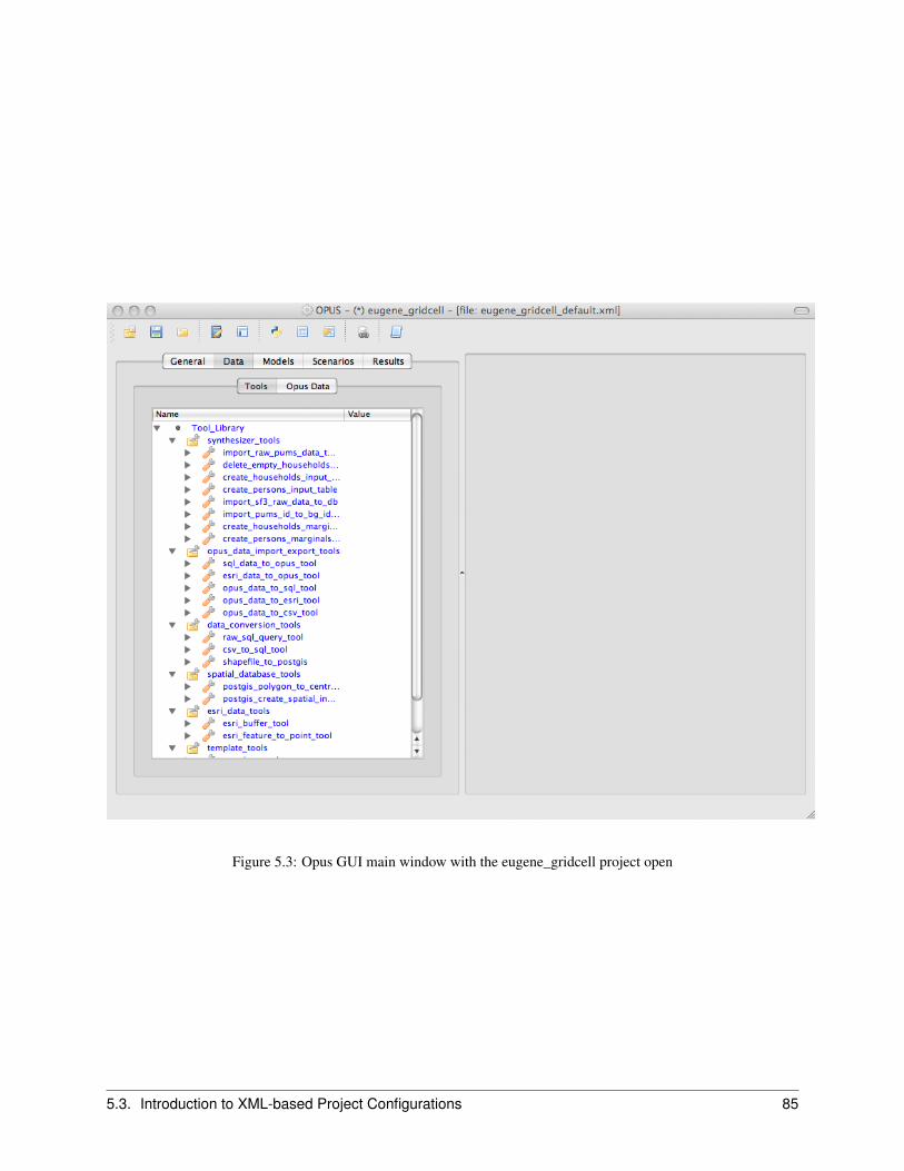
Figure 5.3: Opus GUI main window with the eugene_gridcell project open
5.3. Introduction to XML-based Project Configurations 85

practical terms for a user, this means that you can use default projects as templates, or parents, for another project youwant to create that is mostly the same as an existing project, but has some changes from it. The new project is calleda child project. By default, it inherits all the information contained in the parent project. However, it can override anyinformation inherited from the parent, and add additional information.
Users should create their own projects in the ‘opus/project_configs’ directory. This will allow them to keep projectslocalized in one place, and to avoid editing and possibly corrupting one of the projects that are in an Opus package inthe source code tree.
In fact, the ‘eugene_gridcell_default.xml’ configuration that we just opened initially contains almost no information ofits own — virtually everything is inherited from a parent configuration. As you edit and augment this configuration,more information will be stored in the configuration. It can be saved to disk at any time using the “Save” or “Saveas . . . ” commands on the “File” menu. We suggest saving the configuration under a new name, say ‘my_eugene_-gridcell.xml’, and working from that, so that if you want to start over at some point ‘eugene_gridcell_default.xml’ willstill be there in its original state.
5.4 The Variable Library
Variable in Opus and UrbanSim represent quantities of interest. These variables can be used in two prin-cipal ways: in specifying models and in computing indicators to assess simulation results. For example, adistance_to_highway variable might be used to help predict land values or or household location choices; anda population_density variable might be used in computing indicators that are useful for evaluating simulationresults. The variable library is a repository for variables defined in the system that are accessible from the GUI. Sinceit provides a resource that is used throughout the GUI, we access it from the tools menu on the menu bar at the topof the main window, as in Figure 5.4. The screenshot in Figure 5.5 shows a popup window that appears once a userselects the variable library option on the tools menu. Note that the contents of it depend on what project is loaded. Inthis case, we have the eugene_parcel project loaded, and see the variables that are initially available in this project.
Variables are described in detail later in this manual. Briefly for now, there are three ways to define a variable:
• A variable can be defined using an expression written in a domain-specific programming language. There isa short description of the language later in this chapter. In this chapter we’ll only be looking at defining newvariables in this way.
• A variable can also be a primary attribute of a dataset (think of these as columns in the input database).
• Finally, a variable can be defined as a Python class. This is an advanced option for complicated variables beyondthe scope of the domain-specific programming language — we’ll use variables defined this way that are alreadyin the library, but for now won’t write any new ones.
Note the buttons at the bottom of this window to add new variables or validate all variables. Adding a new variabledefined as an expression is straightforward. There are examples of existing variables defined using expressions in thevariable library window — look for variables with the entry “expression” in the “Source” column. The correspondingvariable definition is in the right-most column. Note that this definition is executable code — it’s not just a description.Expressions are built up as functions and operations applied to existing variables in the library. For example, theexpression for wetland is defined as gridcell.percent_wetland>50. This defines the creation of a true/false,or boolean, variable that is interpreted as 1 if the gridcell has more than 50 percent coverage by wetland, 0 otherwise.Variables are array-valued, so we are actually computing an array of true/false values for every gridcell with the singleexpression.
If you click on the add new variable button at the bottom of the variable library window, it opens a dialog box asshown in Figure 5.6. The top entry is the name you want to use for the variable. Let’s say we want to create a newvariable that is a log of population density. We already have a population density variable defined by gridcell, so wecan just take the log of this value. Let’s name the variable ln_population_density, leave the middle selectionas “expression,” and fill in a simple expression in the definition area: ln(gridcell.population_density).
86 Chapter 5. Software Platform
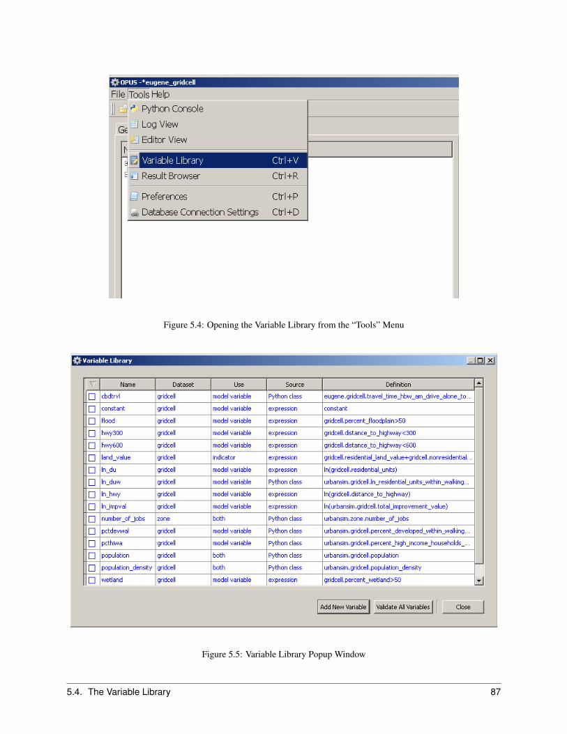
Figure 5.4: Opening the Variable Library from the “Tools” Menu
Figure 5.5: Variable Library Popup Window
5.4. The Variable Library 87
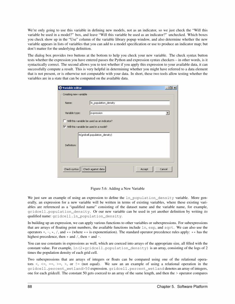
We’re only going to use this variable in defining new models, not as an indicator, so we just check the “Will thisvariable be used in a model?” box, and leave “Will this variable be used as an indicator?” unchecked. Which boxesyou check show up in the “Use” column of the variable library popup window, and also determine whether the newvariable appears in lists of variables that you can add to a model specification or use to produce an indicator map; butdon’t matter for the underlying definition.
The dialog box provides two buttons at the bottom to help you check your new variable. The check syntax buttontests whether the expression you have entered passes the Python and expression syntax checkers – in other words, is itsyntactically correct. The second allows you to test whether if you apply this expression to your available data, it cansuccessfully compute a result. This is very helpful in determining whether you might have referred to a data elementthat is not present, or is otherwise not computable with your data. In short, these two tools allow testing whether thevariables are in a state that can be computed on the available data.
Figure 5.6: Adding a New Variable
We just saw an example of using an expression to define the ln_population_density variable. More gen-erally, an expression for a new variable will be written in terms of existing variables, where these existing vari-ables are referenced as a “qualified name” consisting of the dataset name and the variable name, for example,gridcell.population_density. Or our new variable can be used in yet another definition by writing itsqualified name: gridcell.ln_population_density.
In building up an expression, we can apply various functions to other variables or subexpressions. For subexpressionsthat are arrays of floating point numbers, the available functions include ln, exp, and sqrt. We can also use theoperators +, -, *, /, and ** (where ** is exponentiation). The standard operator precedence rules apply: ** has thehighest precedence, then * and /, then + and -.
You can use constants in expressions as well, which are coerced into arrays of the appropriate size, all filled with theconstant value. For example, ln(2*gridcell.population_density) is an array, consisting of the logs of 2times the population density of each grid cell.
Two subexpressions that are arrays of integers or floats can be compared using one of the relational opera-tors <, <=, ==, >=, >, or != (not equal). We saw an an example of using a relational operation in thegridcell.percent_wetland>50 expression. gridcell.percent_wetland denotes an array of integers,one for each gridcell. The constant 50 gets coerced to an array of the same length, and then the > operator compares
88 Chapter 5. Software Platform
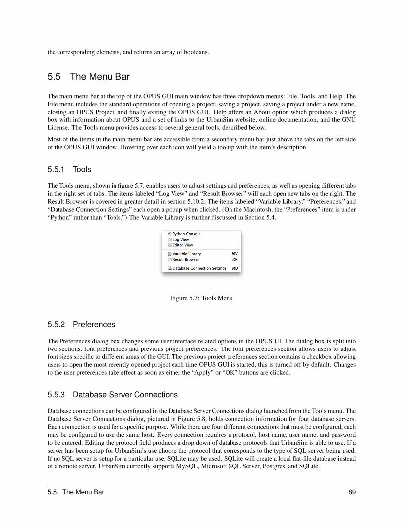
the corresponding elements, and returns an array of booleans.
5.5 The Menu Bar
The main menu bar at the top of the OPUS GUI main window has three dropdown menus: File, Tools, and Help. TheFile menu includes the standard operations of opening a project, saving a project, saving a project under a new name,closing an OPUS Project, and finally exiting the OPUS GUI. Help offers an About option which produces a dialogbox with information about OPUS and a set of links to the UrbanSim website, online documentation, and the GNULicense. The Tools menu provides access to several general tools, described below.
Most of the items in the main menu bar are accessible from a secondary menu bar just above the tabs on the left sideof the OPUS GUI window. Hovering over each icon will yield a tooltip with the item’s description.
5.5.1 Tools
The Tools menu, shown in figure 5.7, enables users to adjust settings and preferences, as well as opening different tabsin the right set of tabs. The items labeled “Log View” and “Result Browser” will each open new tabs on the right. TheResult Browser is covered in greater detail in section 5.10.2. The items labeled “Variable Library,” “Preferences,” and“Database Connection Settings” each open a popup when clicked. (On the Macintosh, the “Preferences” item is under“Python” rather than “Tools.”) The Variable Library is further discussed in Section 5.4.
Figure 5.7: Tools Menu
5.5.2 Preferences
The Preferences dialog box changes some user interface related options in the OPUS UI. The dialog box is split intotwo sections, font preferences and previous project preferences. The font preferences section allows users to adjustfont sizes specific to different areas of the GUI. The previous project preferences section contains a checkbox allowingusers to open the most recently opened project each time OPUS GUI is started, this is turned off by default. Changesto the user preferences take effect as soon as either the “Apply” or “OK” buttons are clicked.
5.5.3 Database Server Connections
Database connections can be configured in the Database Server Connections dialog launched from the Tools menu. TheDatabase Server Connections dialog, pictured in Figure 5.8, holds connection information for four database servers.Each connection is used for a specific purpose. While there are four different connections that must be configured, eachmay be configured to use the same host. Every connection requires a protocol, host name, user name, and passwordto be entered. Editing the protocol field produces a drop down of database protocols that UrbanSim is able to use. If aserver has been setup for UrbanSim’s use choose the protocol that corresponds to the type of SQL server being used.If no SQL server is setup for a particular use, SQLite may be used. SQLite will create a local flat-file database insteadof a remote server. UrbanSim currently supports MySQL, Microsoft SQL Server, Postgres, and SQLite.
5.5. The Menu Bar 89
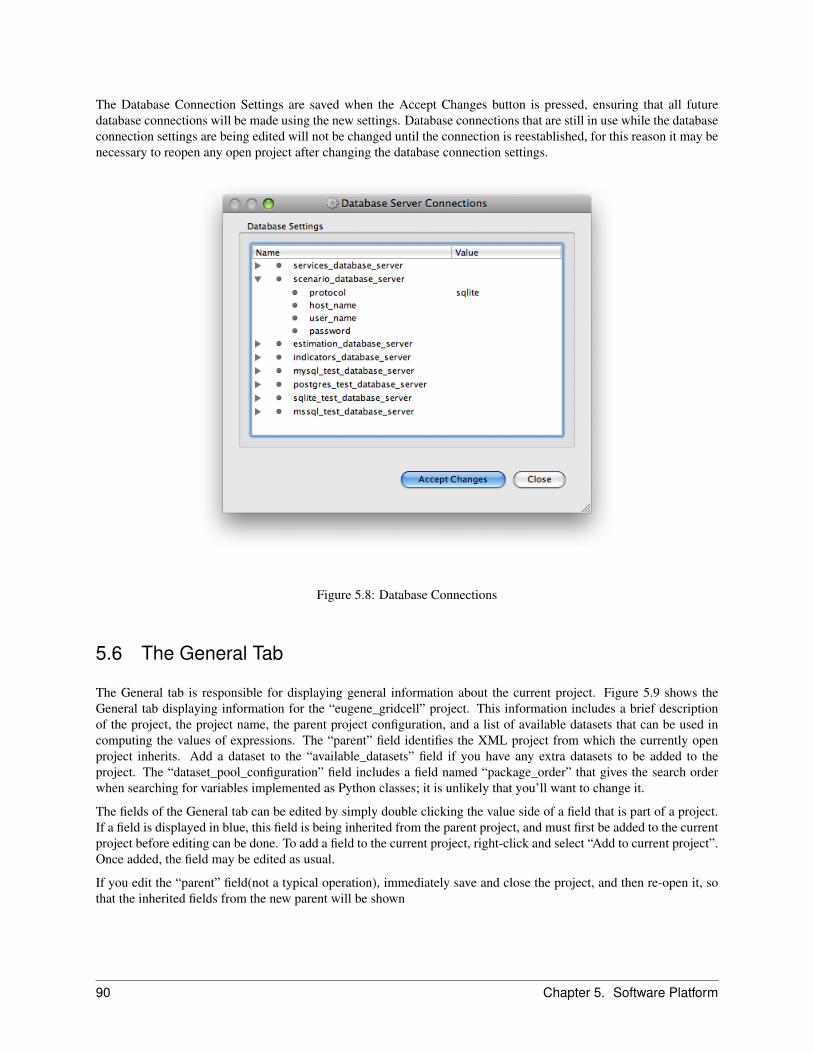
The Database Connection Settings are saved when the Accept Changes button is pressed, ensuring that all futuredatabase connections will be made using the new settings. Database connections that are still in use while the databaseconnection settings are being edited will not be changed until the connection is reestablished, for this reason it may benecessary to reopen any open project after changing the database connection settings.
Figure 5.8: Database Connections
5.6 The General Tab
The General tab is responsible for displaying general information about the current project. Figure 5.9 shows theGeneral tab displaying information for the “eugene_gridcell” project. This information includes a brief descriptionof the project, the project name, the parent project configuration, and a list of available datasets that can be used incomputing the values of expressions. The “parent” field identifies the XML project from which the currently openproject inherits. Add a dataset to the “available_datasets” field if you have any extra datasets to be added to theproject. The “dataset_pool_configuration” field includes a field named “package_order” that gives the search orderwhen searching for variables implemented as Python classes; it is unlikely that you’ll want to change it.
The fields of the General tab can be edited by simply double clicking the value side of a field that is part of a project.If a field is displayed in blue, this field is being inherited from the parent project, and must first be added to the currentproject before editing can be done. To add a field to the current project, right-click and select “Add to current project”.Once added, the field may be edited as usual.
If you edit the “parent” field(not a typical operation), immediately save and close the project, and then re-open it, sothat the inherited fields from the new parent will be shown
90 Chapter 5. Software Platform
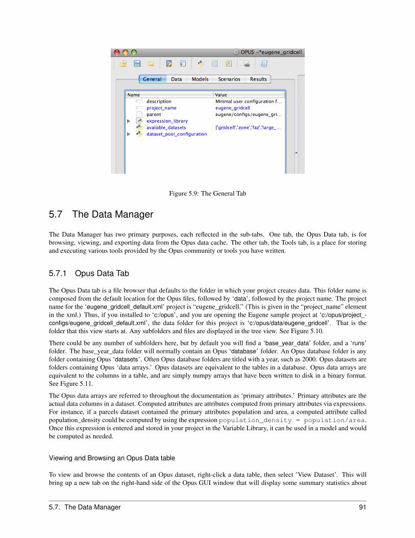
Figure 5.9: The General Tab
5.7 The Data Manager
The Data Manager has two primary purposes, each reflected in the sub-tabs. One tab, the Opus Data tab, is forbrowsing, viewing, and exporting data from the Opus data cache. The other tab, the Tools tab, is a place for storingand executing various tools provided by the Opus community or tools you have written.
5.7.1 Opus Data Tab
The Opus Data tab is a file browser that defaults to the folder in which your project creates data. This folder name iscomposed from the default location for the Opus files, followed by ‘data’, followed by the project name. The projectname for the ‘eugene_gridcell_default.xml’ project is “eugene_gridcell.” (This is given in the “project_name” elementin the xml.) Thus, if you installed to ‘c:/opus’, and you are opening the Eugene sample project at ‘c:/opus/project_-configs/eugene_gridcell_default.xml’, the data folder for this project is ‘c:/opus/data/eugene_gridcell’. That is thefolder that this view starts at. Any subfolders and files are displayed in the tree view. See Figure 5.10.
There could be any number of subfolders here, but by default you will find a ‘base_year_data’ folder, and a ‘runs’folder. The base_year_data folder will normally contain an Opus ‘database’ folder. An Opus database folder is anyfolder containing Opus ‘datasets’. Often Opus database folders are titled with a year, such as 2000. Opus datasets arefolders containing Opus ‘data arrays.’ Opus datasets are equivalent to the tables in a database. Opus data arrays areequivalent to the columns in a table, and are simply numpy arrays that have been written to disk in a binary format.See Figure 5.11.
The Opus data arrays are referred to throughout the documentation as ‘primary attributes.’ Primary attributes are theactual data columns in a dataset. Computed attributes are attributes computed from primary attributes via expressions.For instance, if a parcels dataset contained the primary attributes population and area, a computed attribute calledpopulation_density could be computed by using the expression population_density = population/area.Once this expression is entered and stored in your project in the Variable Library, it can be used in a model and wouldbe computed as needed.
Viewing and Browsing an Opus Data table
To view and browse the contents of an Opus dataset, right-click a data table, then select ’View Dataset’. This willbring up a new tab on the right-hand side of the Opus GUI window that will display some summary statistics about
5.7. The Data Manager 91
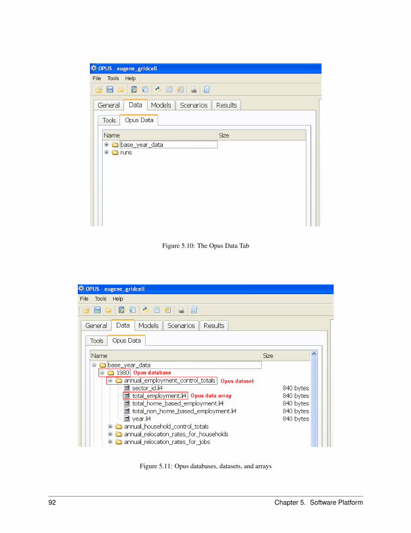
Figure 5.10: The Opus Data Tab
Figure 5.11: Opus databases, datasets, and arrays
92 Chapter 5. Software Platform
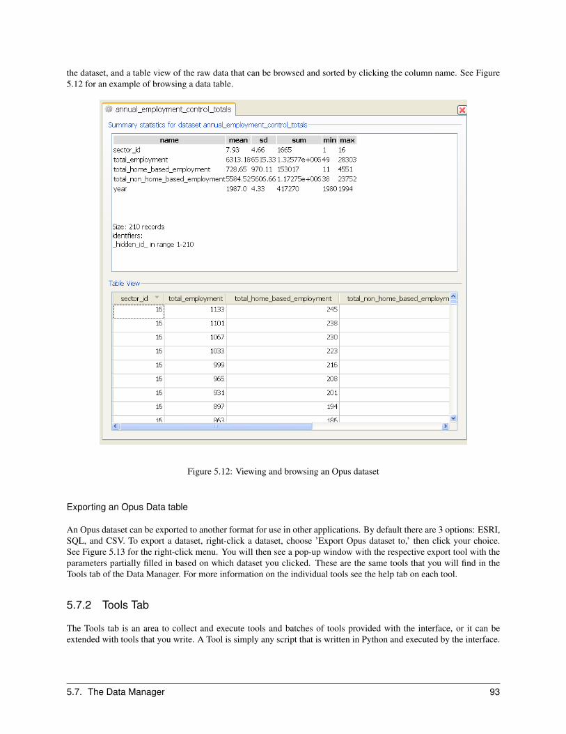
the dataset, and a table view of the raw data that can be browsed and sorted by clicking the column name. See Figure5.12 for an example of browsing a data table.
Figure 5.12: Viewing and browsing an Opus dataset
Exporting an Opus Data table
An Opus dataset can be exported to another format for use in other applications. By default there are 3 options: ESRI,SQL, and CSV. To export a dataset, right-click a dataset, choose ’Export Opus dataset to,’ then click your choice.See Figure 5.13 for the right-click menu. You will then see a pop-up window with the respective export tool with theparameters partially filled in based on which dataset you clicked. These are the same tools that you will find in theTools tab of the Data Manager. For more information on the individual tools see the help tab on each tool.
5.7.2 Tools Tab
The Tools tab is an area to collect and execute tools and batches of tools provided with the interface, or it can beextended with tools that you write. A Tool is simply any script that is written in Python and executed by the interface.
5.7. The Data Manager 93

Figure 5.13: Exporting an Opus dataset
Tool Library
The Tool Library is a place to collect and organize your tools. Tools can also be executed directly from the library in a’one-off’ manner, meaning that you can supply parameters to the tool and execute it without storing those parametersfor future use. To execute a tool from the library, simply right-click it and choose ’Execute Tool...’, see Figure 5.14.This will pop-up a window in which you can supply parameters to the tool then execute it.
New tools can be written and added to the tool library fairly easily. The best way to explain this is to use an example.A ’template_tool’ has been provided so you can see how it works. Feel free to execute the template_tool, it justimplements a simple loop and prints the results to the tool’s log window. The template_tool’s code and associatedXML display everything that is needed to add a tool to the interface. See the code in the source code tree at /opus_-gui/data_manager/run/tools/template_tool.py. A tool also needs XML configuration data in an Opus project. To viewthe XML configuration data for the template_tool, open urbansim.xml in an XML editor from the source code tree at/urbansim/configs and search for template_tool.
At the time of this writing new tools must be placed in the source tree at /opus_gui/data_manager/run/tools in orderto run correctly. There are plans to create an additional ’user tools’ folder where tools could also be placed. Also, atthis moment, the XML must be hand written to ensure that the tools show up properly in the interface and executecorrectly. There are some right-click functions in the Tool Library to assist with the XML editing (to add a new tool,create parameters for it, etc.) but these functions are in a beta state.
Once a new tool and its associated XML is written properly, the Tool Library will display the tool and dynamicallypopulate the pop-up dialog box with the proper parameters based on the XML configuration. The tools are quiteflexible. Although the initial tool must be written using Python, there is no limit placed upon what one can do.For starters, there are tools provided in the interface that make OS calls to external executables (e.g. ogr2ogr.exe),databases, and myriad other libraries to accomplish various tasks (e.g. ESRI geoprocessing). Feel free to browse thesource code for any provided tool along with the XML configuration to see some possibilities.
94 Chapter 5. Software Platform

Figure 5.14: Executing a tool
Tool Sets
Tool Sets are simply collections of tools from the Tool Library with parameters stored so they can be executed re-peatedly or in order in a batch manner. Tool Sets can contain any number of tools from the Library. A new Tool Setcan be created by right-clicking Tool_Sets and choosing ’Add new tool set.’ This adds a new Tool Set to the bottomof the list. It can be renamed by double-clicking it and typing in a name, taking care to not use spaces or a leadinginteger as these are invalid in XML nodes. Once you have a new Tool Set, tools from the Library can be added to it byright-clicking a Tool Set and choosing ’Add Tool to Tool set.’ See Figure 5.15 for an example of what this looks like.
From this window, choose a tool from the drop down menu, fill in the parameters, then click ’Add Tool.’ The tool isadded to the Tool Set and the parameters you entered are stored in the project XML file. This configured tool can nowbe executed by itself with those parameters, or executed as part of a batch in the Tool Set. Tools in a Tool Set can bere-ordered by right-clicking them and choosing to move them up or down, and all of the tools can be executed in theorder they appear by right-clicking a Tool Set and choosing ’Execute Tool Set’.
5.8 The Models Manager
The model manager tab in the GUI provides the functionality to create models of various types, configure them, specifythe variables to use in them, and then estimate their parameters if they have a form that needs to be estimated – suchas regression models or discrete choice models.
5.8.1 Creating an Allocation Model
To demonstrate the process of creating models in the GUI, let’s begin with a simple allocation model, which does nothave any parameters to estimate and represents a straightforward model to configure. Say we want to create a modelthat allocates home-based jobs to zones, and lack sufficient data to specify a choice model or regression model for thispurpose. Home-based jobs are those jobs that are located in properties that are residential in character. Assume thatwe have no behavioral information about this problem, other than the insight that home-based jobs are... home-based.So we can infer that we should probably allocate these jobs to places that have housing (or households). In allocatingthese jobs to zones (traffic analysis zones used in the travel model), we can count how many residential units are in
5.8. The Models Manager 95
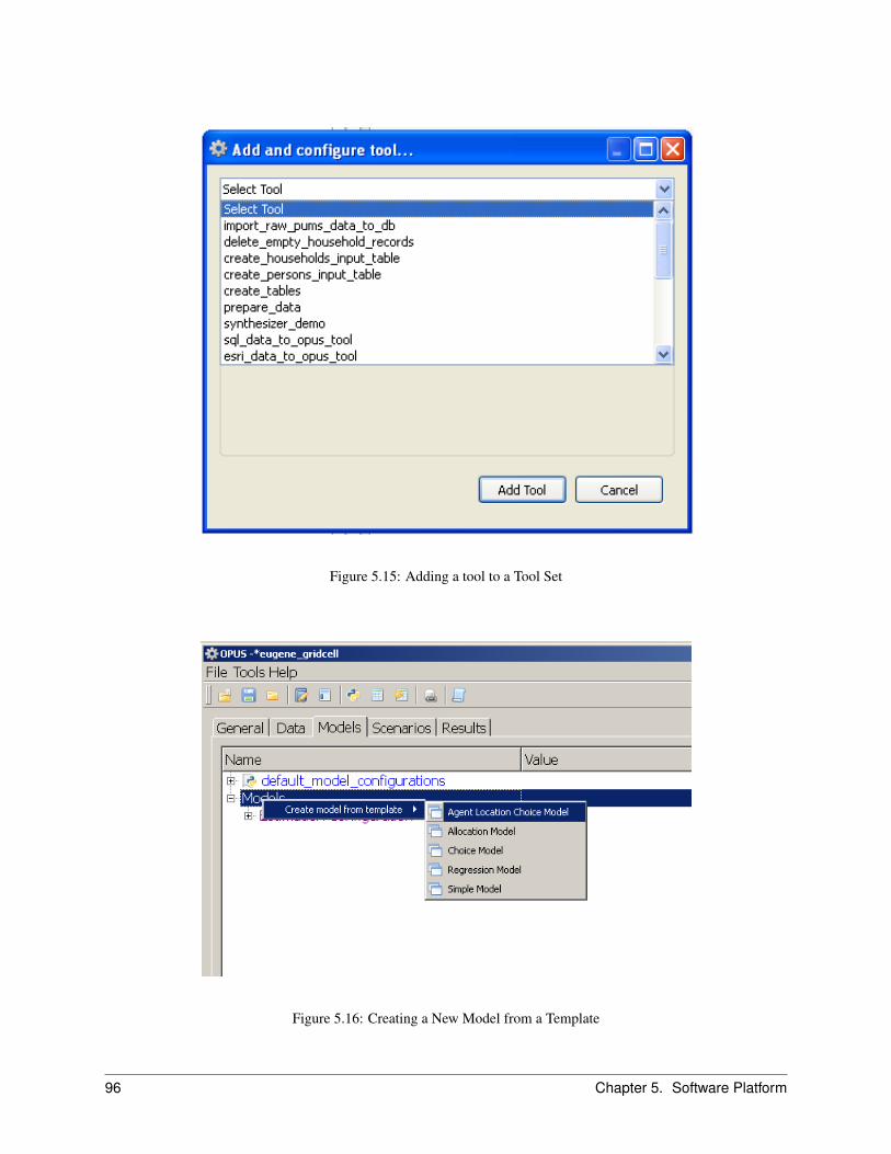
Figure 5.15: Adding a tool to a Tool Set
Figure 5.16: Creating a New Model from a Template
96 Chapter 5. Software Platform
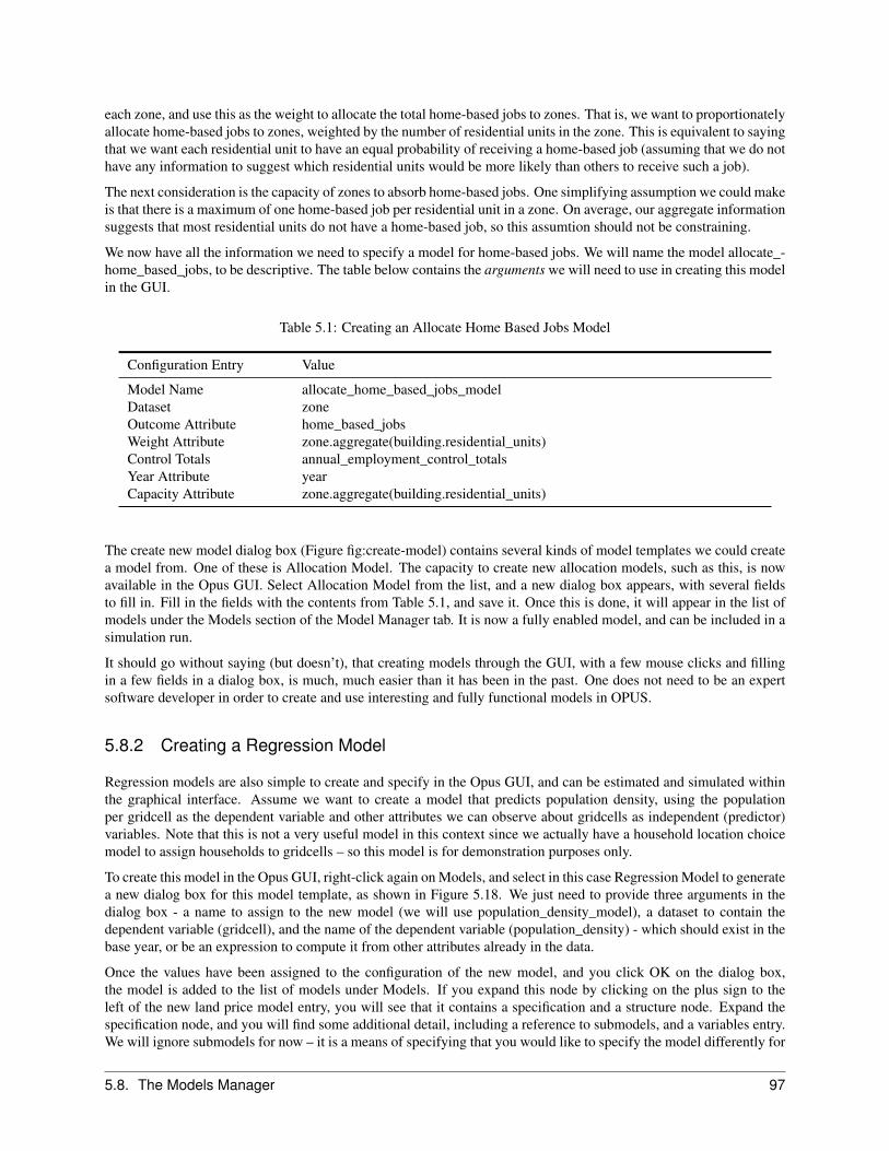
each zone, and use this as the weight to allocate the total home-based jobs to zones. That is, we want to proportionatelyallocate home-based jobs to zones, weighted by the number of residential units in the zone. This is equivalent to sayingthat we want each residential unit to have an equal probability of receiving a home-based job (assuming that we do nothave any information to suggest which residential units would be more likely than others to receive such a job).
The next consideration is the capacity of zones to absorb home-based jobs. One simplifying assumption we could makeis that there is a maximum of one home-based job per residential unit in a zone. On average, our aggregate informationsuggests that most residential units do not have a home-based job, so this assumtion should not be constraining.
We now have all the information we need to specify a model for home-based jobs. We will name the model allocate_-home_based_jobs, to be descriptive. The table below contains the arguments we will need to use in creating this modelin the GUI.
Table 5.1: Creating an Allocate Home Based Jobs Model
Configuration Entry Value
Model Name allocate_home_based_jobs_modelDataset zoneOutcome Attribute home_based_jobsWeight Attribute zone.aggregate(building.residential_units)Control Totals annual_employment_control_totalsYear Attribute yearCapacity Attribute zone.aggregate(building.residential_units)
The create new model dialog box (Figure fig:create-model) contains several kinds of model templates we could createa model from. One of these is Allocation Model. The capacity to create new allocation models, such as this, is nowavailable in the Opus GUI. Select Allocation Model from the list, and a new dialog box appears, with several fieldsto fill in. Fill in the fields with the contents from Table 5.1, and save it. Once this is done, it will appear in the list ofmodels under the Models section of the Model Manager tab. It is now a fully enabled model, and can be included in asimulation run.
It should go without saying (but doesn’t), that creating models through the GUI, with a few mouse clicks and fillingin a few fields in a dialog box, is much, much easier than it has been in the past. One does not need to be an expertsoftware developer in order to create and use interesting and fully functional models in OPUS.
5.8.2 Creating a Regression Model
Regression models are also simple to create and specify in the Opus GUI, and can be estimated and simulated withinthe graphical interface. Assume we want to create a model that predicts population density, using the populationper gridcell as the dependent variable and other attributes we can observe about gridcells as independent (predictor)variables. Note that this is not a very useful model in this context since we actually have a household location choicemodel to assign households to gridcells – so this model is for demonstration purposes only.
To create this model in the Opus GUI, right-click again on Models, and select in this case Regression Model to generatea new dialog box for this model template, as shown in Figure 5.18. We just need to provide three arguments in thedialog box - a name to assign to the new model (we will use population_density_model), a dataset to contain thedependent variable (gridcell), and the name of the dependent variable (population_density) - which should exist in thebase year, or be an expression to compute it from other attributes already in the data.
Once the values have been assigned to the configuration of the new model, and you click OK on the dialog box,the model is added to the list of models under Models. If you expand this node by clicking on the plus sign to theleft of the new land price model entry, you will see that it contains a specification and a structure node. Expand thespecification node, and you will find some additional detail, including a reference to submodels, and a variables entry.We will ignore submodels for now – it is a means of specifying that you would like to specify the model differently for
5.8. The Models Manager 97
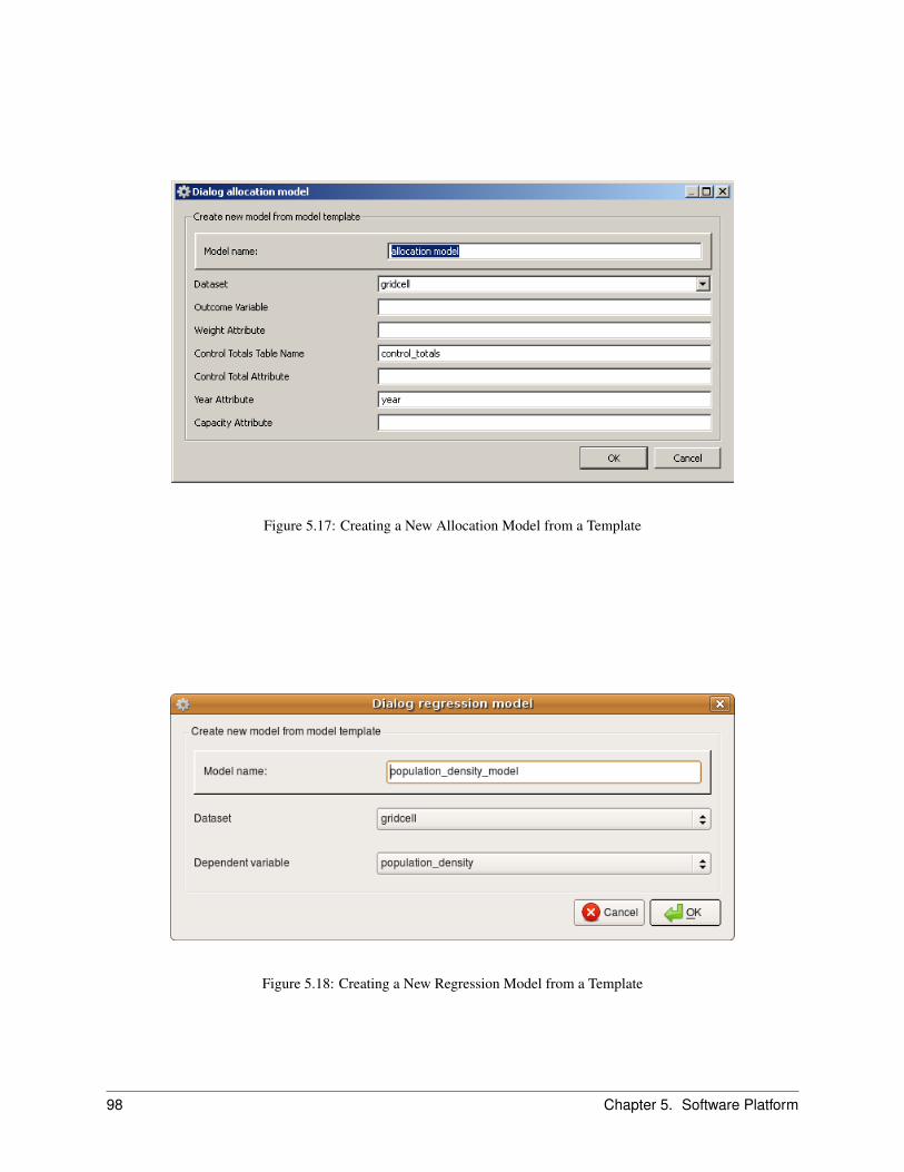
Figure 5.17: Creating a New Allocation Model from a Template
Figure 5.18: Creating a New Regression Model from a Template
98 Chapter 5. Software Platform
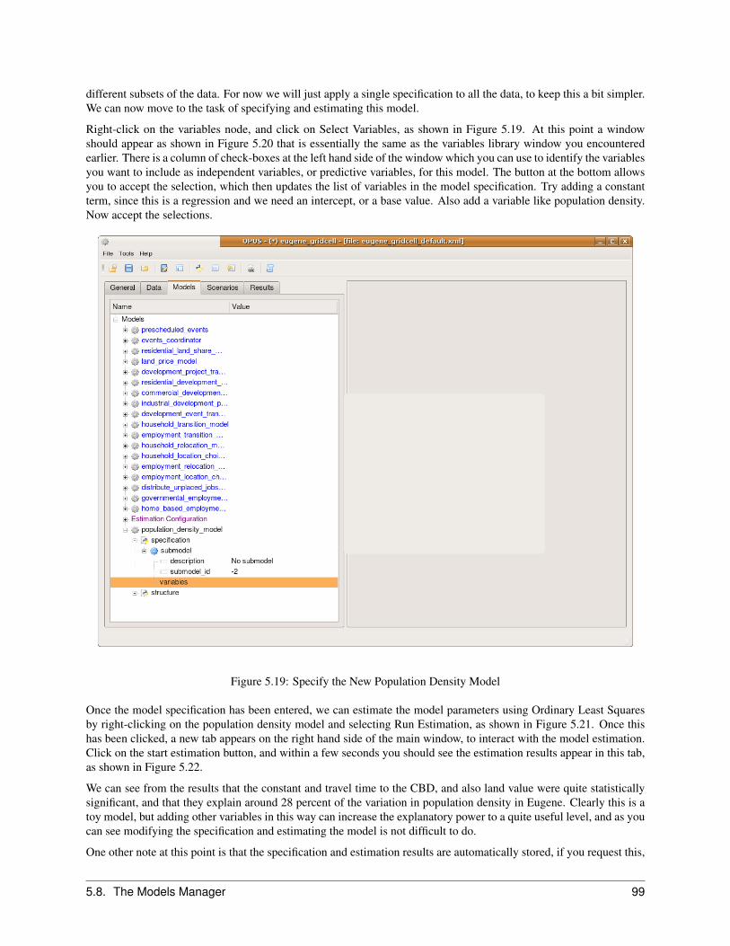
different subsets of the data. For now we will just apply a single specification to all the data, to keep this a bit simpler.We can now move to the task of specifying and estimating this model.
Right-click on the variables node, and click on Select Variables, as shown in Figure 5.19. At this point a windowshould appear as shown in Figure 5.20 that is essentially the same as the variables library window you encounteredearlier. There is a column of check-boxes at the left hand side of the window which you can use to identify the variablesyou want to include as independent variables, or predictive variables, for this model. The button at the bottom allowsyou to accept the selection, which then updates the list of variables in the model specification. Try adding a constantterm, since this is a regression and we need an intercept, or a base value. Also add a variable like population density.Now accept the selections.
Figure 5.19: Specify the New Population Density Model
Once the model specification has been entered, we can estimate the model parameters using Ordinary Least Squaresby right-clicking on the population density model and selecting Run Estimation, as shown in Figure 5.21. Once thishas been clicked, a new tab appears on the right hand side of the main window, to interact with the model estimation.Click on the start estimation button, and within a few seconds you should see the estimation results appear in this tab,as shown in Figure 5.22.
We can see from the results that the constant and travel time to the CBD, and also land value were quite statisticallysignificant, and that they explain around 28 percent of the variation in population density in Eugene. Clearly this is atoy model, but adding other variables in this way can increase the explanatory power to a quite useful level, and as youcan see modifying the specification and estimating the model is not difficult to do.
One other note at this point is that the specification and estimation results are automatically stored, if you request this,
5.8. The Models Manager 99
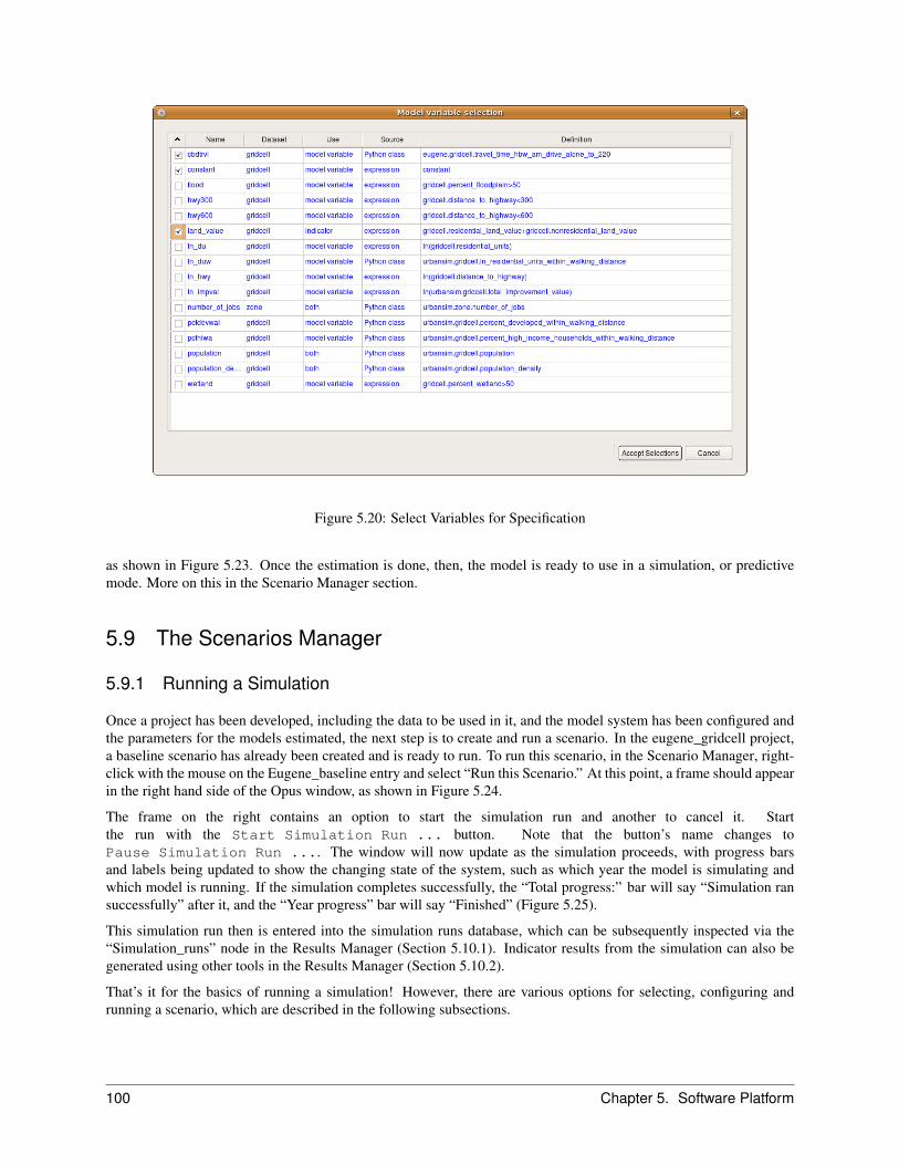
Figure 5.20: Select Variables for Specification
as shown in Figure 5.23. Once the estimation is done, then, the model is ready to use in a simulation, or predictivemode. More on this in the Scenario Manager section.
5.9 The Scenarios Manager
5.9.1 Running a Simulation
Once a project has been developed, including the data to be used in it, and the model system has been configured andthe parameters for the models estimated, the next step is to create and run a scenario. In the eugene_gridcell project,a baseline scenario has already been created and is ready to run. To run this scenario, in the Scenario Manager, right-click with the mouse on the Eugene_baseline entry and select “Run this Scenario.” At this point, a frame should appearin the right hand side of the Opus window, as shown in Figure 5.24.
The frame on the right contains an option to start the simulation run and another to cancel it. Startthe run with the Start Simulation Run ... button. Note that the button’s name changes toPause Simulation Run .... The window will now update as the simulation proceeds, with progress barsand labels being updated to show the changing state of the system, such as which year the model is simulating andwhich model is running. If the simulation completes successfully, the “Total progress:” bar will say “Simulation ransuccessfully” after it, and the “Year progress” bar will say “Finished” (Figure 5.25).
This simulation run then is entered into the simulation runs database, which can be subsequently inspected via the“Simulation_runs” node in the Results Manager (Section 5.10.1). Indicator results from the simulation can also begenerated using other tools in the Results Manager (Section 5.10.2).
That’s it for the basics of running a simulation! However, there are various options for selecting, configuring andrunning a scenario, which are described in the following subsections.
100 Chapter 5. Software Platform
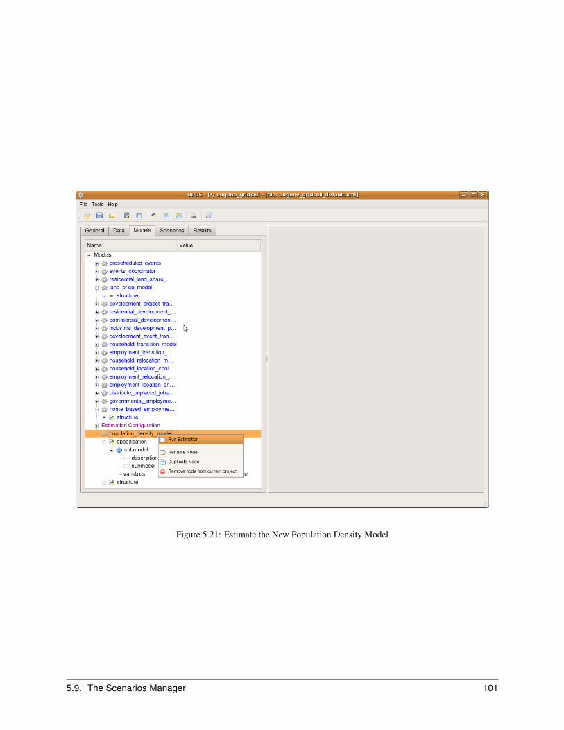
Figure 5.21: Estimate the New Population Density Model
5.9. The Scenarios Manager 101
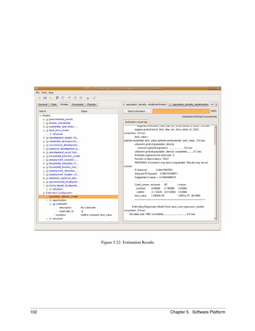
Figure 5.22: Estimation Results
102 Chapter 5. Software Platform
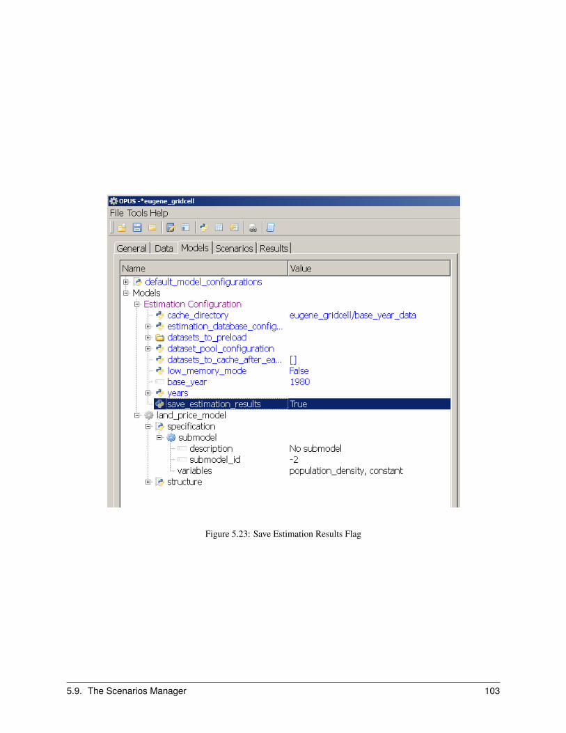
Figure 5.23: Save Estimation Results Flag
5.9. The Scenarios Manager 103
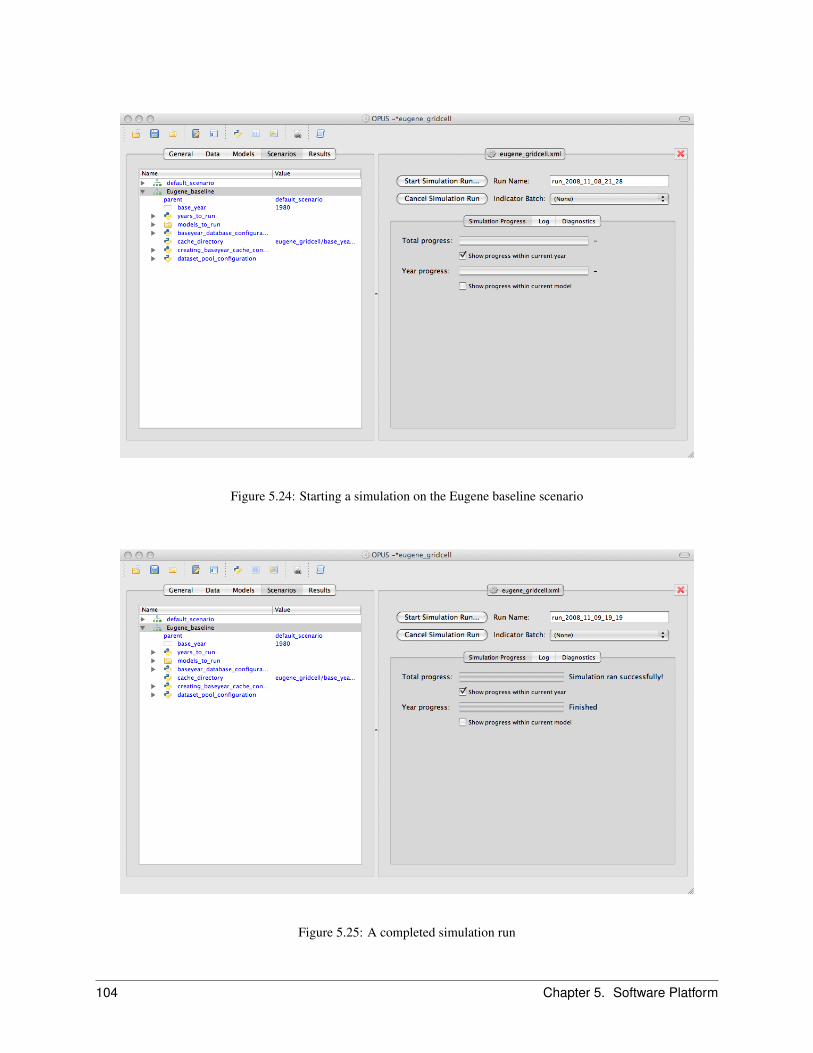
Figure 5.24: Starting a simulation on the Eugene baseline scenario
Figure 5.25: A completed simulation run
104 Chapter 5. Software Platform
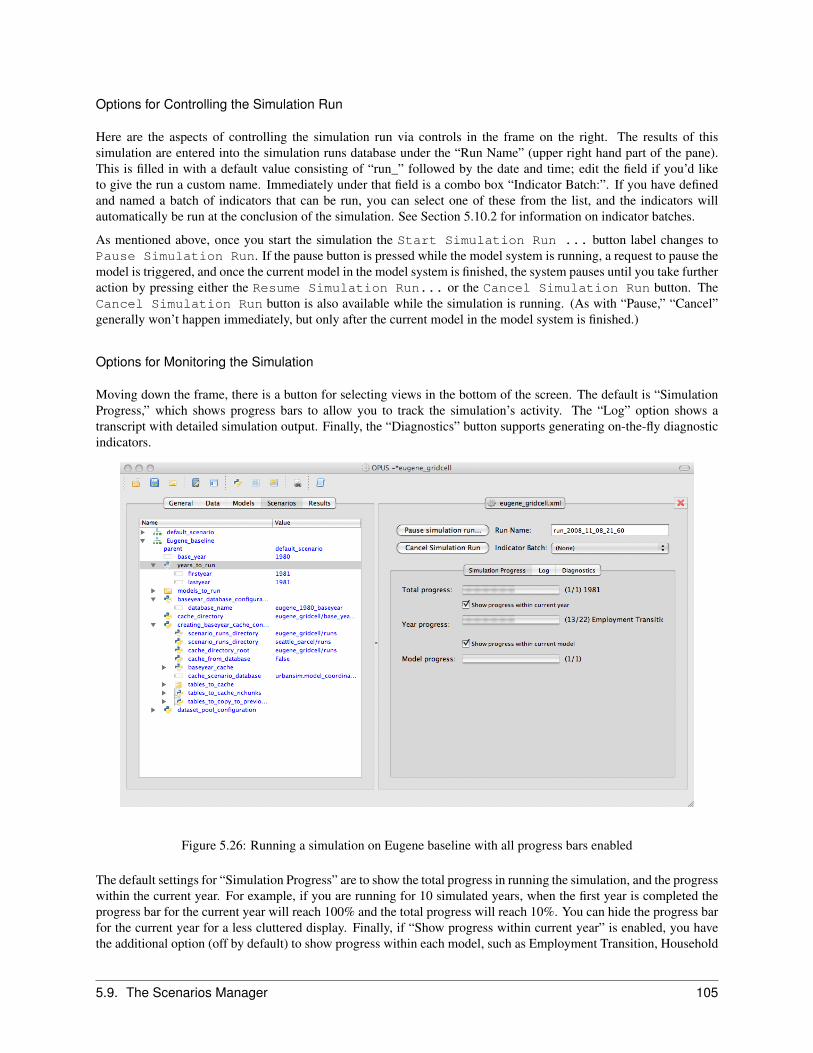
Options for Controlling the Simulation Run
Here are the aspects of controlling the simulation run via controls in the frame on the right. The results of thissimulation are entered into the simulation runs database under the “Run Name” (upper right hand part of the pane).This is filled in with a default value consisting of “run_” followed by the date and time; edit the field if you’d liketo give the run a custom name. Immediately under that field is a combo box “Indicator Batch:”. If you have definedand named a batch of indicators that can be run, you can select one of these from the list, and the indicators willautomatically be run at the conclusion of the simulation. See Section 5.10.2 for information on indicator batches.
As mentioned above, once you start the simulation the Start Simulation Run ... button label changes toPause Simulation Run. If the pause button is pressed while the model system is running, a request to pause themodel is triggered, and once the current model in the model system is finished, the system pauses until you take furtheraction by pressing either the Resume Simulation Run... or the Cancel Simulation Run button. TheCancel Simulation Run button is also available while the simulation is running. (As with “Pause,” “Cancel”generally won’t happen immediately, but only after the current model in the model system is finished.)
Options for Monitoring the Simulation
Moving down the frame, there is a button for selecting views in the bottom of the screen. The default is “SimulationProgress,” which shows progress bars to allow you to track the simulation’s activity. The “Log” option shows atranscript with detailed simulation output. Finally, the “Diagnostics” button supports generating on-the-fly diagnosticindicators.
Figure 5.26: Running a simulation on Eugene baseline with all progress bars enabled
The default settings for “Simulation Progress” are to show the total progress in running the simulation, and the progresswithin the current year. For example, if you are running for 10 simulated years, when the first year is completed theprogress bar for the current year will reach 100% and the total progress will reach 10%. You can hide the progress barfor the current year for a less cluttered display. Finally, if “Show progress within current year” is enabled, you havethe additional option (off by default) to show progress within each model, such as Employment Transition, Household
5.9. The Scenarios Manager 105
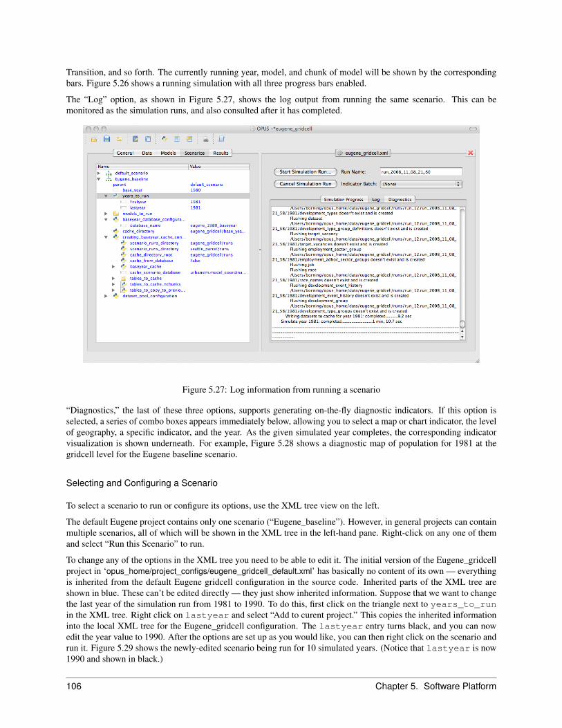
Transition, and so forth. The currently running year, model, and chunk of model will be shown by the correspondingbars. Figure 5.26 shows a running simulation with all three progress bars enabled.
The “Log” option, as shown in Figure 5.27, shows the log output from running the same scenario. This can bemonitored as the simulation runs, and also consulted after it has completed.
Figure 5.27: Log information from running a scenario
“Diagnostics,” the last of these three options, supports generating on-the-fly diagnostic indicators. If this option isselected, a series of combo boxes appears immediately below, allowing you to select a map or chart indicator, the levelof geography, a specific indicator, and the year. As the given simulated year completes, the corresponding indicatorvisualization is shown underneath. For example, Figure 5.28 shows a diagnostic map of population for 1981 at thegridcell level for the Eugene baseline scenario.
Selecting and Configuring a Scenario
To select a scenario to run or configure its options, use the XML tree view on the left.
The default Eugene project contains only one scenario (“Eugene_baseline”). However, in general projects can containmultiple scenarios, all of which will be shown in the XML tree in the left-hand pane. Right-click on any one of themand select “Run this Scenario” to run.
To change any of the options in the XML tree you need to be able to edit it. The initial version of the Eugene_gridcellproject in ‘opus_home/project_configs/eugene_gridcell_default.xml’ has basically no content of its own — everythingis inherited from the default Eugene gridcell configuration in the source code. Inherited parts of the XML tree areshown in blue. These can’t be edited directly — they just show inherited information. Suppose that we want to changethe last year of the simulation run from 1981 to 1990. To do this, first click on the triangle next to years_to_runin the XML tree. Right click on lastyear and select “Add to curent project.” This copies the inherited informationinto the local XML tree for the Eugene_gridcell configuration. The lastyear entry turns black, and you can nowedit the year value to 1990. After the options are set up as you would like, you can then right click on the scenario andrun it. Figure 5.29 shows the newly-edited scenario being run for 10 simulated years. (Notice that lastyear is now1990 and shown in black.)
106 Chapter 5. Software Platform
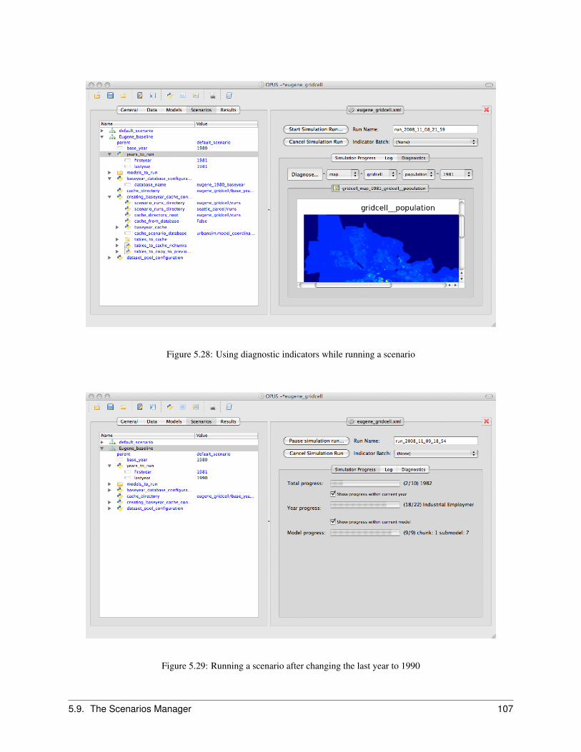
Figure 5.28: Using diagnostic indicators while running a scenario
Figure 5.29: Running a scenario after changing the last year to 1990
5.9. The Scenarios Manager 107
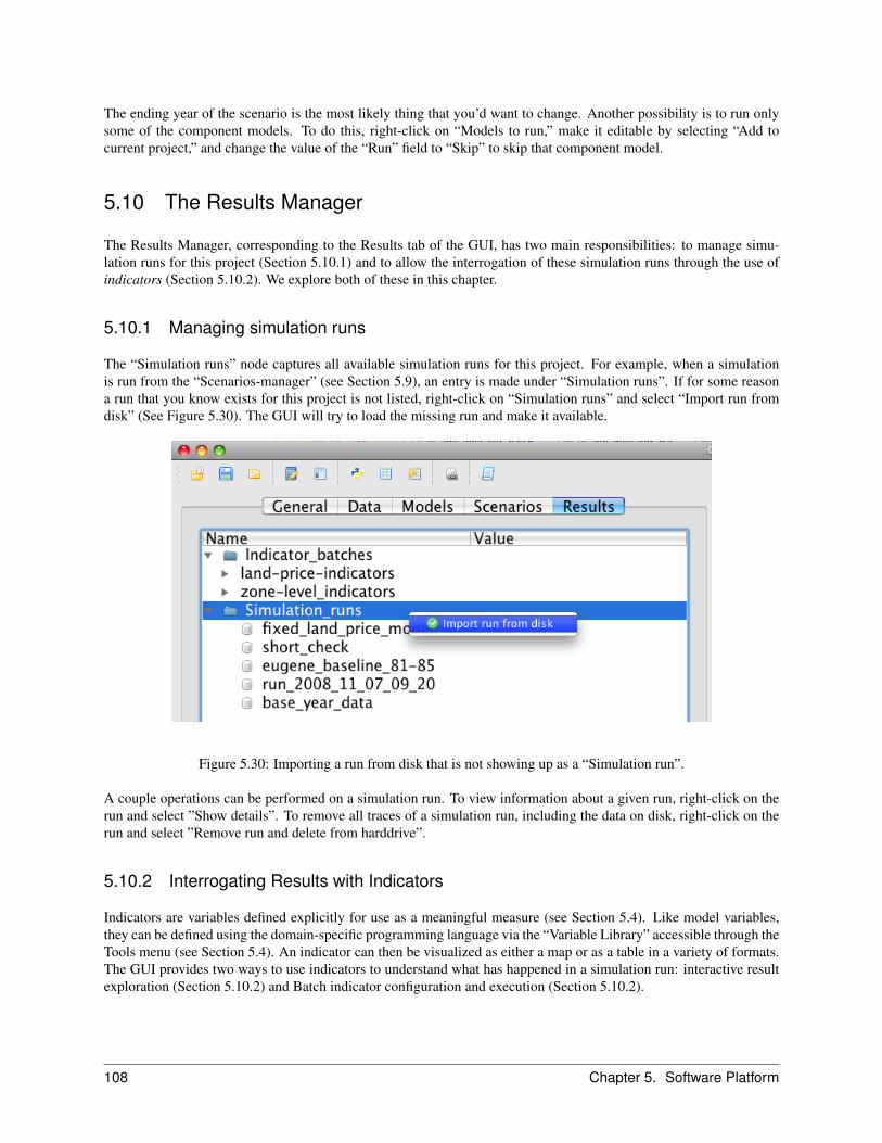
The ending year of the scenario is the most likely thing that you’d want to change. Another possibility is to run onlysome of the component models. To do this, right-click on “Models to run,” make it editable by selecting “Add tocurrent project,” and change the value of the “Run” field to “Skip” to skip that component model.
5.10 The Results Manager
The Results Manager, corresponding to the Results tab of the GUI, has two main responsibilities: to manage simu-lation runs for this project (Section 5.10.1) and to allow the interrogation of these simulation runs through the use ofindicators (Section 5.10.2). We explore both of these in this chapter.
5.10.1 Managing simulation runs
The “Simulation runs” node captures all available simulation runs for this project. For example, when a simulationis run from the “Scenarios-manager” (see Section 5.9), an entry is made under “Simulation runs”. If for some reasona run that you know exists for this project is not listed, right-click on “Simulation runs” and select “Import run fromdisk” (See Figure 5.30). The GUI will try to load the missing run and make it available.
Figure 5.30: Importing a run from disk that is not showing up as a “Simulation run”.
A couple operations can be performed on a simulation run. To view information about a given run, right-click on therun and select ”Show details”. To remove all traces of a simulation run, including the data on disk, right-click on therun and select ”Remove run and delete from harddrive”.
5.10.2 Interrogating Results with Indicators
Indicators are variables defined explicitly for use as a meaningful measure (see Section 5.4). Like model variables,they can be defined using the domain-specific programming language via the “Variable Library” accessible through theTools menu (see Section 5.4). An indicator can then be visualized as either a map or as a table in a variety of formats.The GUI provides two ways to use indicators to understand what has happened in a simulation run: interactive resultexploration (Section 5.10.2) and Batch indicator configuration and execution (Section 5.10.2).
108 Chapter 5. Software Platform

Interactive result exploration
Often, it is desirable to explore simulation results in a lightweight fashion in order to get a basic idea of what happened.You don’t necessarily want to go through the process of exporting results to a GIS mapping tool in order to gain somebasic intuitions into spatial patterns.
The Opus GUI’s “Result Browser”, available from the “tools” menu, allows interactive exploration of simulationresults. The Result Browser presents a selectable list of available simulation runs, years over which those simulationswere run, and available indicators. You can then configure an indicator visualization by selecting a simulation run, ayear, and an indicator. To compute and visualize the configured indicator, simply press the “generate results” button(See Figure 5.31). The indicator will then be computed for the year of the selected simulation run. After it is computed,a tab should appear at the bottom of the window with the name of the indicator. Subtabs allow you to see the resultsas a table or map (using the Matplotlib Python module).
Figure 5.31: Using the “Result browser” for interactive result exploration.
1. Open the Results Browser from the Tools menu. Usethe Results Browser to answer the following ques-tions.
2. Just from visual inspection, is there more than onecluster of gridcells with high land value in the Eu-gene region in 1980 in the baseyear data?
3. Is this cluster(s) in the same general area as the great-est number of jobs in Eugene for the same year of thebaseyear data?
5.10. The Results Manager 109
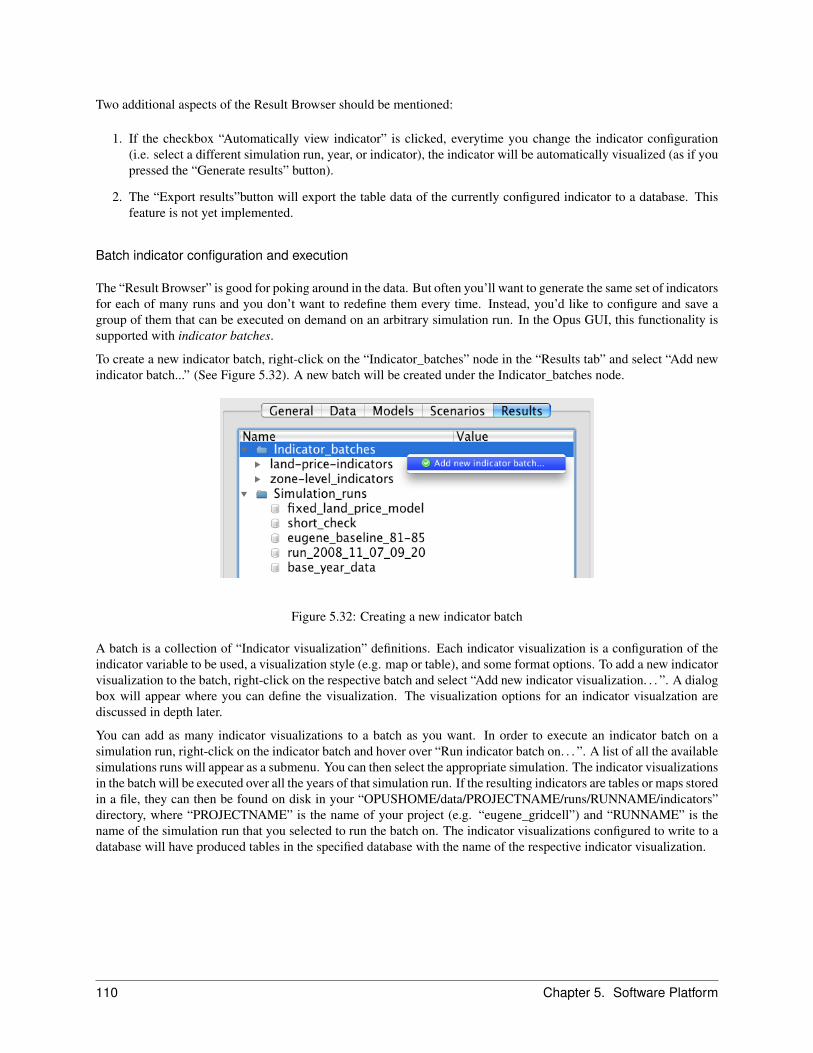
Two additional aspects of the Result Browser should be mentioned:
1. If the checkbox “Automatically view indicator” is clicked, everytime you change the indicator configuration(i.e. select a different simulation run, year, or indicator), the indicator will be automatically visualized (as if youpressed the “Generate results” button).
2. The “Export results”button will export the table data of the currently configured indicator to a database. Thisfeature is not yet implemented.
Batch indicator configuration and execution
The “Result Browser” is good for poking around in the data. But often you’ll want to generate the same set of indicatorsfor each of many runs and you don’t want to redefine them every time. Instead, you’d like to configure and save agroup of them that can be executed on demand on an arbitrary simulation run. In the Opus GUI, this functionality issupported with indicator batches.
To create a new indicator batch, right-click on the “Indicator_batches” node in the “Results tab” and select “Add newindicator batch...” (See Figure 5.32). A new batch will be created under the Indicator_batches node.
Figure 5.32: Creating a new indicator batch
A batch is a collection of “Indicator visualization” definitions. Each indicator visualization is a configuration of theindicator variable to be used, a visualization style (e.g. map or table), and some format options. To add a new indicatorvisualization to the batch, right-click on the respective batch and select “Add new indicator visualization. . . ”. A dialogbox will appear where you can define the visualization. The visualization options for an indicator visualzation arediscussed in depth later.
You can add as many indicator visualizations to a batch as you want. In order to execute an indicator batch on asimulation run, right-click on the indicator batch and hover over “Run indicator batch on. . . ”. A list of all the availablesimulations runs will appear as a submenu. You can then select the appropriate simulation. The indicator visualizationsin the batch will be executed over all the years of that simulation run. If the resulting indicators are tables or maps storedin a file, they can then be found on disk in your “OPUSHOME/data/PROJECTNAME/runs/RUNNAME/indicators”directory, where “PROJECTNAME” is the name of your project (e.g. “eugene_gridcell”) and “RUNNAME” is thename of the simulation run that you selected to run the batch on. The indicator visualizations configured to write to adatabase will have produced tables in the specified database with the name of the respective indicator visualization.
110 Chapter 5. Software Platform
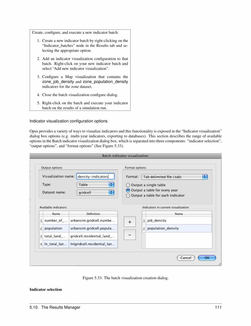
Create, configure, and execute a new indicator batch:
1. Create a new indicator batch by right-clicking on the“Indicator_batches” node in the Results tab and se-lecting the appropriate option.
2. Add an indicator visualization configuration to thatbatch. Right-click on your new indicator batch andselect “Add new indicator visualization”.
3. Configure a Map visualization that contains thezone_job_density and zone_population_densityindicators for the zone dataset.
4. Close the batch visualization configure dialog.
5. Right-click on the batch and execute your indicatorbatch on the results of a simulation run.
Indicator visualization configuration options
Opus provides a variety of ways to visualize indicators and this functionality is exposed in the “Indicator visualization”dialog box options (e.g. multi-year indicators, exporting to databases). This section describes the range of availableoptions in the Batch indicator visualization dialog box, which is separated into three components: “indicator selection”,“output options”, and “format options” (See Figure 5.33).
Figure 5.33: The batch visualization creation dialog.
Indicator selection
5.10. The Results Manager 111

The bottom of the dialog box has two list boxes, “available indicators” and “indicators in current visualization”. Theindicators here are those variables defined in the “Variable Library” (see Section 5.4) whose use has been set to beindicator or both. Note that the set of indicators available is filtered by the currently selected dataset in the “outputoptions” (described later in this section).
By moving an indicator from the “available indicators” box to the “indicators in current visualization” bo via the“+” button, you include that indicator in this indicator visualization. Likewise, to remove an indicator from thevisualization, select the indicator in the “indicators in current visualization” box and press the “-” button.
Output options
Visualization Name. The base name of any produced visualizations. Because you might be producing this visualizationfor different years and different simulation data, more information will be appended to this name to ensure uniquenessof the resulting file or database table when the visualization is run on some data.
Type. There are two different types of indicator visualizations that can be produced: maps and tables. Tables arejust raw data organized into rows and columns, while maps are spatial projections of this data. The available formatoptions (described later) are fully dependent on the visualization type.
Dataset name. The dataset that this visualization corresponds to. When the selected indicator(s) are run, they will becomputed over this dataset. Most commonly you are choosing a geographic granularity (e.g. gridcell, zone) that youwant to see the results at. Note that when you change the dataset, the set of available indicators changes because agiven indicator is valid only for a single dataset.
Format options for maps
Map visualizations will produce a map file for every selected indicator for every available year when it is executed ona simulation run.
The available map format is Mapnik, an open-source toolkit for developing mapping applications (http://mapnik.org/). Note that the Mapnik maps are not intended to replace GIS-based mapping, which allows farmore control and the overlay of other features for visual reference. It is merely a quick tool to visualize data to geta sense of the spatial patterns in it. In order to support visualization in a GIS environment such as ArcGIS or QGIS,the results may be exported to a database or geodatabase environment, and the GIS software used to create a moreinteractive and flexible display of the data. See the following section for a description of how to export indicator resultsto a SQL database or a DBF file for use in external GIS tools.
112 Chapter 5. Software Platform

Export the results that were found in the previous tutorialinset to a SQL database.
1. Make sure that you have configured a databaseserver. From the Tools menu, select “DatabaseServer Connections”. Check to see that the “indi-cators_database_server” is correctly set up. If youdon’t have a remote database server, make sure thatit points to a sqlite connection. Close the connectionsdialog box.
2. Reconfigure the batch to write to a database. Expandthe indicator batch that you defined in the prior step.Right-click on the visualization and select “Config-ure visualization”. Change the format to “Export toSQL database” and then name a database it shouldwrite to. Hit OK and then rerun the batch on the sim-ulation results from before.
3. Launch a database browser and check to see if theproper tables were created.
To set the Mapnik map options, first open the batch visualization creation dialog window (shown above) by clicking onthe Results tab, right-clicking “Indicator_batches”, selecting the “Add new indicator batch. . . ” option, right-clickingthe new indicator batch, and selecting the “Add new indicator visualization. . . ” option. Select “Map” from the “Type:”drop-down menu, then click the “Mapnik Map Options” button that will appear directly below the “Format:” drop-down menu. In the Mapnik Map Options dialog window, there are two tabs where all of the mapping options can beset: Legend Options and Size Options.
5.10. The Results Manager 113

Legend Options tab:
Figure 5.34: The map options dialog window showing default settings (Legend Options).
Number of Color Ranges. This sets the number of buckets to split the range of the values being mapped in to. Thedrop-down menu allows you to choose a number between 1 and 10.
Color Scaling Type. This drop-down menu allows you to choose between “Linear Scaling”, “Custom Scaling”, “Cus-tom Linear Scaling”, and “Equal Percentage Scaling”. Linear scaling will evenly divide of the range of values to bemapped into buckets of the same size. Custom scaling will let you specify how to divide the range of values into thebuckets. Custom linear scaling will let you specify a minimum and maximum value and then will evenly divide therange of values into buckets of the same size. Equal Percentage Scaling will divide the range of values up so that(100/number of buckets) percent of the values fall into each category.
Custom Scale. If “Custom Scaling” is selected as the Color Scaling Type, then the values in this text field will be usedto define the bucket ranges. For example, if the following string is entered in the Custom Scale text field “5, 100, 2000,40000”, then the bucket ranges will be ’5 to 100’, ’100 to 2000’, and ’2000 to 40000’. Also, if either “min”, “MIN”,“max”, or “MAX” is entered in the Custom Scale text field, they will be replaced with the minimum or maximumvalues of the values that are being mapped. For example, ”min,100,max” is a valid entry for Custom Scale.
Label Type. This drop-down menu allows you to choose between “Range Values” and “Custom Labels” to use as thelabels on the color bar that will be drawn in to the map image. Using range values means that the boxes in the colorbar will be labeled with the range of values that are being colored with the color contained in the corresponding box.Using custom labels allows you to manually enter the labels for each box.
Custom Labels. If “Custom Labels” is selected as the Label Type, then the values in this text field will be used to
114 Chapter 5. Software Platform

label the colored boxes in the color bar. For example, if the following string is entered in the Custom Labels text field“a,b,c,”, then the first box will be labeled “a”, the second will be labeled “b”, and the third will be labeled “c”.
Color Scheme. This drop-down menu allows you to choose between “Custom Color Scheme”, ”Green”, “Blue”,“Red”, and “Custom Graduated Colors”. The color buttons in the legend are buttons, that when pushed, cause a colorchooser dialog window to pop up that can be used to pick the color of the box. If Custom Color Scheme is selected,then all manually-set colors will be saved when the “Apply Changes” button is pushed, whereas all colors will beover-written when the “Apply Changes” button is clicked if any other color scheme option is selected. If Green, Blue,or Red is selected, the boxes will be colored with pre-defined colors. Lastly, if Custom Graduated Colors is selected,then the boxes will be colored in an even, graduated scale where the range of colors starts at the current color of thebox at index 1 and ends at the current color of the box at the highest index.
Diverge Colors On. This gives you the option to have two diverging colors. You have to option “None” to split onnone of the indices to use just one color scale, or you have the option to split on any index from 1 to 10. The colorbox at the selected index will be set to white and the two color scales above and below it will be set based on whatcolor option is selected in the Color Scheme and Diverging Color drop-down menus. Note that if “Custom GraduatedColors” is selected in the Color Scheme drop-down menu, then the two color scales above and below the box at thediverging index will have graduated color scales and the option selected in the Diverging Color drop-down menu willbe ignored.
Diverging Color. This drop-down menu allows you to choose between “Red”, “Green”, and “Blue”. This will set thecolor for the boxes with an index number lower than the index number selected in the Diverge Colors On drop-downmenu. Note: any selection made in this menu will be ignored if “Custom Color Scheme” is selected in the ColorScheme drop-down menu.
Legend. The legend has three columns: Color, Range, and Label. The Color column has color boxes that display thecolor currently selected for the corresponding color bucket. Also, clicking a color box will bring up a dialog windowthat will allow you to select a custom color to display on the color box. The Range column has numerical values thatdefine the range of the corresponding color bucket and these values can be edited within the legend table if “CustomScaling” is selected in the Color Scaling Type drop-down menu. The Label column has the label that will be appliedto each color bucket on the color bar that will be included in the map. These values are editable from within the legendtable if “Custom Labels” is selected in the Label Type drop-down menu. Note: values entered in the legend table willonly be saved correctly if they appear correctly in the Custom Scale and Custom Labels text fields.
5.10. The Results Manager 115
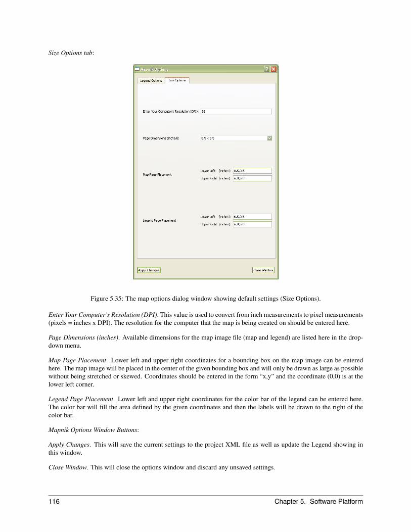
Size Options tab:
Figure 5.35: The map options dialog window showing default settings (Size Options).
Enter Your Computer’s Resolution (DPI). This value is used to convert from inch measurements to pixel measurements(pixels = inches x DPI). The resolution for the computer that the map is being created on should be entered here.
Page Dimensions (inches). Available dimensions for the map image file (map and legend) are listed here in the drop-down menu.
Map Page Placement. Lower left and upper right coordinates for a bounding box on the map image can be enteredhere. The map image will be placed in the center of the given bounding box and will only be drawn as large as possiblewithout being stretched or skewed. Coordinates should be entered in the form “x,y” and the coordinate (0,0) is at thelower left corner.
Legend Page Placement. Lower left and upper right coordinates for the color bar of the legend can be entered here.The color bar will fill the area defined by the given coordinates and then the labels will be drawn to the right of thecolor bar.
Mapnik Options Window Buttons:
Apply Changes. This will save the current settings to the project XML file as well as update the Legend showing inthis window.
Close Window. This will close the options window and discard any unsaved settings.
116 Chapter 5. Software Platform
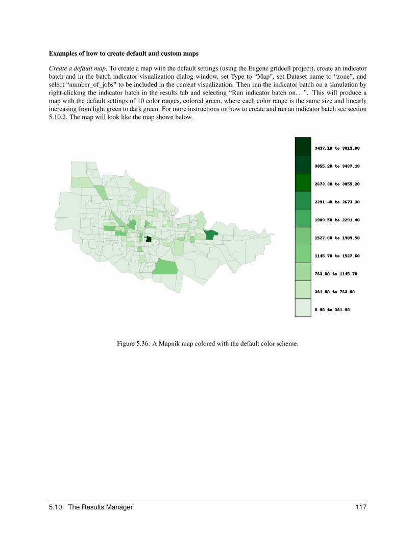
Examples of how to create default and custom maps
Create a default map. To create a map with the default settings (using the Eugene gridcell project), create an indicatorbatch and in the batch indicator visualization dialog window, set Type to “Map”, set Dataset name to “zone”, andselect “number_of_jobs” to be included in the current visualization. Then run the indicator batch on a simulation byright-clicking the indicator batch in the results tab and selecting “Run indicator batch on. . . ”. This will produce amap with the default settings of 10 color ranges, colored green, where each color range is the same size and linearlyincreasing from light green to dark green. For more instructions on how to create and run an indicator batch see section5.10.2. The map will look like the map shown below.
Figure 5.36: A Mapnik map colored with the default color scheme.
5.10. The Results Manager 117
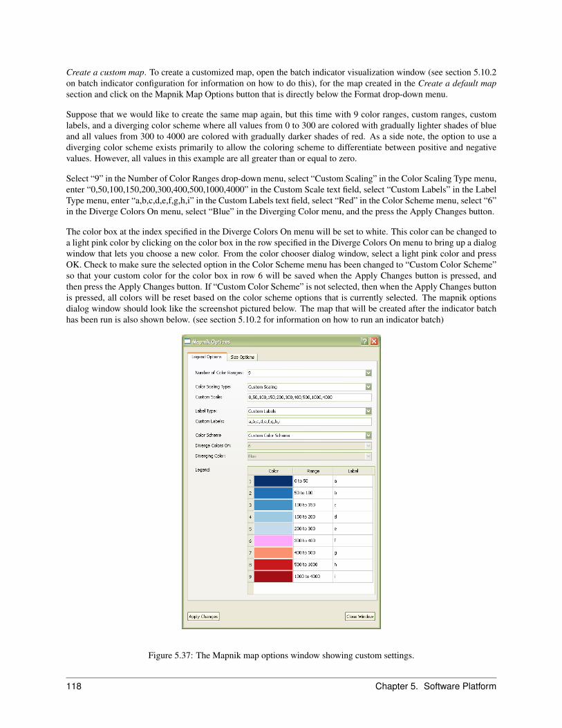
Create a custom map. To create a customized map, open the batch indicator visualization window (see section 5.10.2on batch indicator configuration for information on how to do this), for the map created in the Create a default mapsection and click on the Mapnik Map Options button that is directly below the Format drop-down menu.
Suppose that we would like to create the same map again, but this time with 9 color ranges, custom ranges, customlabels, and a diverging color scheme where all values from 0 to 300 are colored with gradually lighter shades of blueand all values from 300 to 4000 are colored with gradually darker shades of red. As a side note, the option to use adiverging color scheme exists primarily to allow the coloring scheme to differentiate between positive and negativevalues. However, all values in this example are all greater than or equal to zero.
Select “9” in the Number of Color Ranges drop-down menu, select “Custom Scaling” in the Color Scaling Type menu,enter “0,50,100,150,200,300,400,500,1000,4000” in the Custom Scale text field, select “Custom Labels” in the LabelType menu, enter “a,b,c,d,e,f,g,h,i” in the Custom Labels text field, select “Red” in the Color Scheme menu, select “6”in the Diverge Colors On menu, select “Blue” in the Diverging Color menu, and the press the Apply Changes button.
The color box at the index specified in the Diverge Colors On menu will be set to white. This color can be changed toa light pink color by clicking on the color box in the row specified in the Diverge Colors On menu to bring up a dialogwindow that lets you choose a new color. From the color chooser dialog window, select a light pink color and pressOK. Check to make sure the selected option in the Color Scheme menu has been changed to “Custom Color Scheme”so that your custom color for the color box in row 6 will be saved when the Apply Changes button is pressed, andthen press the Apply Changes button. If “Custom Color Scheme” is not selected, then when the Apply Changes buttonis pressed, all colors will be reset based on the color scheme options that is currently selected. The mapnik optionsdialog window should look like the screenshot pictured below. The map that will be created after the indicator batchhas been run is also shown below. (see section 5.10.2 for information on how to run an indicator batch)
Figure 5.37: The Mapnik map options window showing custom settings.
118 Chapter 5. Software Platform
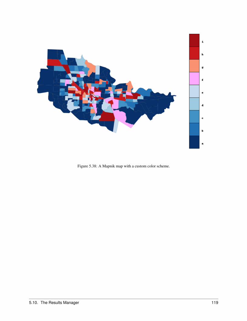
Figure 5.38: A Mapnik map with a custom color scheme.
5.10. The Results Manager 119
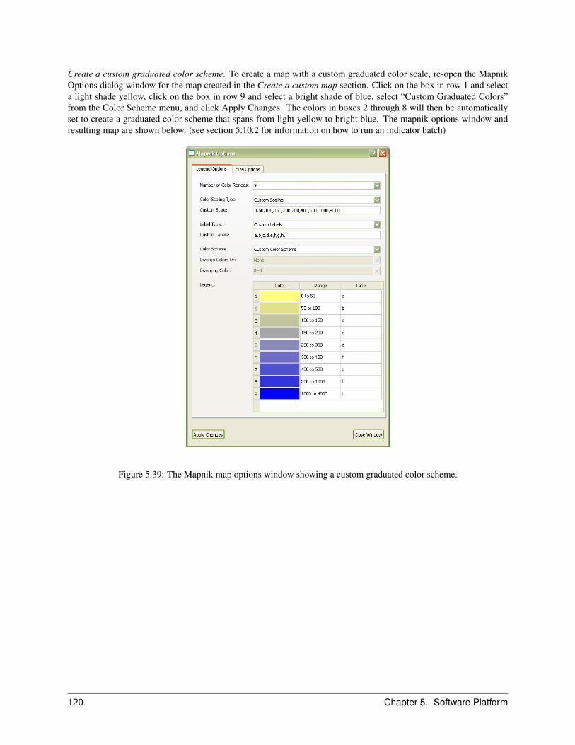
Create a custom graduated color scheme. To create a map with a custom graduated color scale, re-open the MapnikOptions dialog window for the map created in the Create a custom map section. Click on the box in row 1 and selecta light shade yellow, click on the box in row 9 and select a bright shade of blue, select “Custom Graduated Colors”from the Color Scheme menu, and click Apply Changes. The colors in boxes 2 through 8 will then be automaticallyset to create a graduated color scheme that spans from light yellow to bright blue. The mapnik options window andresulting map are shown below. (see section 5.10.2 for information on how to run an indicator batch)
Figure 5.39: The Mapnik map options window showing a custom graduated color scheme.
120 Chapter 5. Software Platform

Figure 5.40: A Mapnik map with a custom graduated color scheme.
5.10. The Results Manager 121
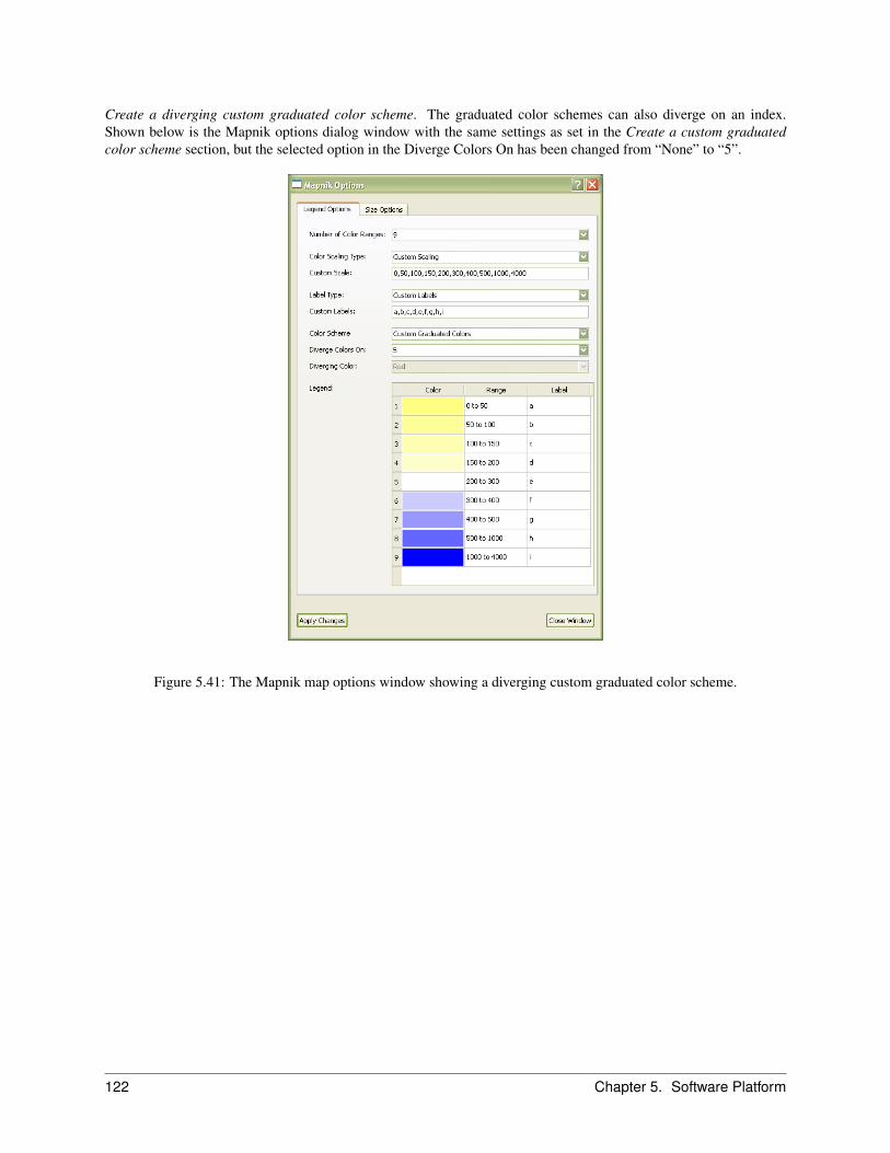
Create a diverging custom graduated color scheme. The graduated color schemes can also diverge on an index.Shown below is the Mapnik options dialog window with the same settings as set in the Create a custom graduatedcolor scheme section, but the selected option in the Diverge Colors On has been changed from “None” to “5”.
Figure 5.41: The Mapnik map options window showing a diverging custom graduated color scheme.
122 Chapter 5. Software Platform
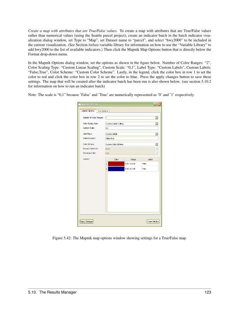
Create a map with attributes that are True/False values. To create a map with attributes that are True/False valuesrather than numerical values (using the Seattle parcel project), create an indicator batch in the batch indicator visu-alization dialog window, set Type to “Map”, set Dataset name to “parcel”, and select “hwy2000” to be included inthe current visualization. (See Section /refsec:variable-library for information on how to use the “Variable Library” toadd hwy2000 to the list of available indicators.) Then click the Mapnik Map Options button that is directly below theFormat drop-down menu.
In the Mapnik Options dialog window, set the options as shown in the figure below. Number of Color Ranges: “2”,Color Scaling Type: “Custom Linear Scaling”, Custom Scale: “0,1”, Label Type: “Custom Labels”, Custom Labels:“False,True”, Color Scheme: “Custom Color Scheme”. Lastly, in the legend, click the color box in row 1 to set thecolor to red and click the color box in row 2 to set the color to blue. Press the apply changes button to save thesesettings. The map that will be created after the indicator batch has been run is also shown below. (see section 5.10.2for information on how to run an indicator batch)
Note: The scale is “0,1” because ’False’ and ’True’ are numerically represented as ’0’ and ’1’ respectively.
Figure 5.42: The Mapnik map options window showing settings for a True/False map.
5.10. The Results Manager 123
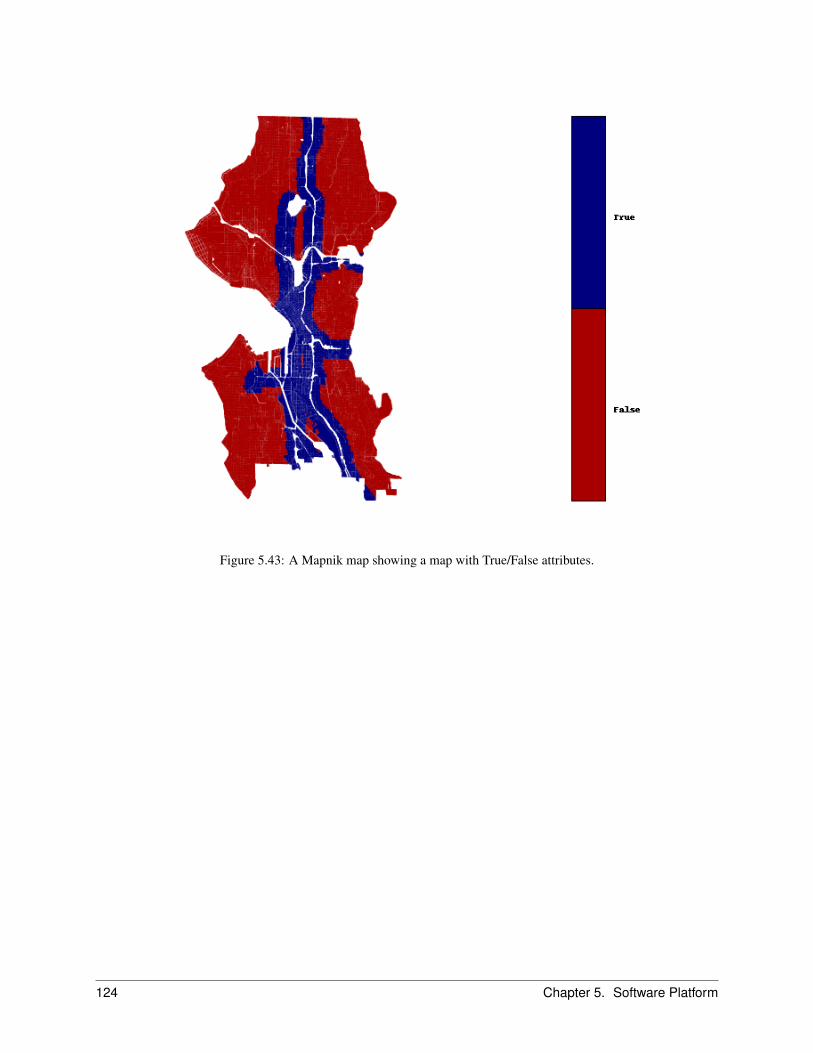
Figure 5.43: A Mapnik map showing a map with True/False attributes.
124 Chapter 5. Software Platform

Format options for animations
Animation visualizations will produce an animation file for every selected indicator that repeatedly loops through mapimages that correspond to the years the batch was selected to run on when it is executed on a simulation run.
The available animation format is Mapnik, an open-source toolkit for developing mapping applications (http://mapnik.org/).
To set the Mapnik map options, first open the batch visualization creation dialog window by clicking on the Results tab,right-clicking “Indicator_batches”, selecting the “Add new indicator batch...” option, right-clicking the new indicatorbatch, and selecting the “Add new indicator visualization...” option. Select “Animation” from the “Type:” drop-downmenu, then click the “Mapnik Map Options” button that will appear directly below the “Format:” drop-down menu.In the Mapnik Map Options dialog window, all of the animation options can be set.
All of the animated map options are the same as the non-animated map options. See the above section on formatoptions for maps for more info.
Format options for tables
There are four different available formats for tables. Each has its own parameters that need to be set. Note that the idcolumn for the dataset will automatically be included in all outputted tables regardless of format.
Tab-delimited (.tab). This will output a file (or multiple files) where the values are separated by tabs. There arethree different modes to choose from that affects how data is split across files when the visualization is executed ona simulation run. “Output in a single file” will create single tab file that has a column for each selected indicator foreach year of the simulation run. “Output in a table for every year” will create a tab file for each year of the simulationrun, with each column corresponding to a selected indicator. Finally, “Output a table for each indicator” will create atab file for each selected indicator, where each column corresponds to the indicator values of a year of the simulationrun.
Fixed-field. The fixed field format will output a single file whose fields are written with fixed width and no delimiters.The file contains a column for each selected indicator for each year of the simulation run for which the visualizationis being created. Format info for each column needs to be specified. To specify the format of the dataset id column,fill in the “id_col” input field. To specify the format of each selected indicator, enter the format in the respective rowof the “field format” column in the “indicators in current visualization” box. The field format has two parts, the lengthof the field and the type. Available types are float ( “f”) and integer ( “i”). Specified field formats follow the pattern“10i” and “5.2f”, where the latter specifies a float with five leading digits with floating point precision carried out totwo decimal places.
SQL database. This format option can be used to export to an arbitrary SQL database. The database server usedis that specified in the “Database server connections” under “indicators_database” (see Section 5.5.3). The exporteddata will take the form of a newly created in the specified database (if the database doesn’t exist, it will be createdfirst). The SQL table will contain a column for every selected indicator for every year of the simulation run that itis being executed against. The name of the table is a combination of the name of the visualization and the nameof the simulation run. Additionally, if you are exporting to a PostGRES database and have an existing spatial tablecorresponding to the dataset of the visualization, a view defining a join over the spatial table and the indicator tablewill automatically be created. This allows you to instantly view the indicator results in QGIS.
ESRI database. This option exports the indicator data to an ESRI database that can be loaded into ArcMap. Simplyspecify the path to a geodatabase file (.gdb). It is assumed that the geodatabase contains a Feature Class corre-sponding to the dataset of the indicator being exported. Once the export is successfully completed, the geodatabasewill contain a table that contains the indicator result, with a zone_id and an ArcGIS OBJECTID* that corresponds tothe internal object ids in the feature class. It is safe to join the indicator table result with the feature class using eitherthe objectid or the zone_id. See Figure 5.44 for an example exported indicator after following this process.
5.10. The Results Manager 125
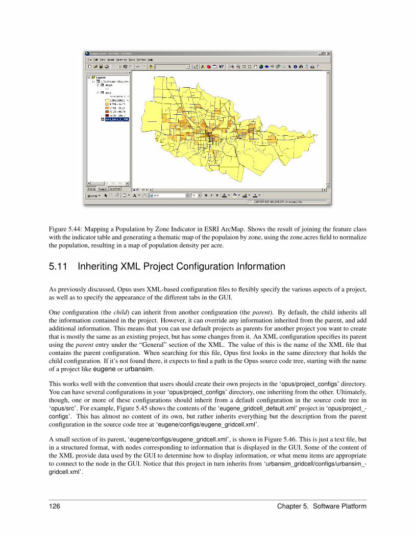
Figure 5.44: Mapping a Population by Zone Indicator in ESRI ArcMap. Shows the result of joining the feature classwith the indicator table and generating a thematic map of the populaion by zone, using the zone.acres field to normalizethe population, resulting in a map of population density per acre.
5.11 Inheriting XML Project Configuration Information
As previously discussed, Opus uses XML-based configuration files to flexibly specify the various aspects of a project,as well as to specify the appearance of the different tabs in the GUI.
One configuration (the child) can inherit from another configuration (the parent). By default, the child inherits allthe information contained in the project. However, it can override any information inherited from the parent, and addadditional information. This means that you can use default projects as parents for another project you want to createthat is mostly the same as an existing project, but has some changes from it. An XML configuration specifies its parentusing the parent entry under the “General” section of the XML. The value of this is the name of the XML file thatcontains the parent configuration. When searching for this file, Opus first looks in the same directory that holds thechild configuration. If it’s not found there, it expects to find a path in the Opus source code tree, starting with the nameof a project like eugene or urbansim.
This works well with the convention that users should create their own projects in the ‘opus/project_configs’ directory.You can have several configurations in your ‘opus/project_configs’ directory, one inheriting from the other. Ultimately,though, one or more of these configurations should inherit from a default configuration in the source code tree in‘opus/src’. For example, Figure 5.45 shows the contents of the ‘eugene_gridcell_default.xml’ project in ‘opus/project_-configs’. This has almost no content of its own, but rather inherits everything but the description from the parentconfiguration in the source code tree at ‘eugene/configs/eugene_gridcell.xml’.
A small section of its parent, ‘eugene/configs/eugene_gridcell.xml’, is shown in Figure 5.46. This is just a text file, butin a structured format, with nodes corresponding to information that is displayed in the GUI. Some of the content ofthe XML provide data used by the GUI to determine how to display information, or what menu items are appropriateto connect to the node in the GUI. Notice that this project in turn inherits from ‘urbansim_gridcell/configs/urbansim_-gridcell.xml’.
126 Chapter 5. Software Platform

<opus_project><xml_version>4.2.0</xml_version><general>
<description type="string">Minimal user configuration for the Eugene gridcell project</description><parent type="file">eugene/configs/eugene_gridcell.xml</parent>
</general></opus_project>
Figure 5.45: Contents of the default eugene_gridcell.xml project
Figure 5.46: An Excerpt from eugene/configs/eugene_gridcell.xml
5.11. Inheriting XML Project Configuration Information 127

To change any of the options in the XML tree you need to be able to edit it. Inherited parts of the XML tree are shownin blue in the left pane in the GUI. These can’t be edited directly — they just show inherited information. You canmake an inherited portion of the XML tree editable by right clicking on it and selecting “Add to curent project.” Thiscopies the inherited information into the local XML tree, which then is shown in black. We saw an example of doingthis in Section 5.9.1. Figure 5.29 in that same section shows an XML tree that is mostly inherited (and so shown inblue).
A few details about the “Add to current project” command: in Section 5.9.1, when we added lastyear to thecurrent project, the containing nodes in the tree (years_to_run and Eugene_baseline) also turned black,since they needed to be added to the current project as well to hold lastyear. It’s also possible to click directly onyears_to_run, or even Eugene_baseline, and add the XML tree under that to the current project. However,we recommend adding just the part you’re editing to the current project, and not others. (You can always add otherparts later.) The reason is that once a part of the tree is added to the current project, the inheritance relation of thatpart with the parent disappears, and changes to the parent won’t be reflected in the child XML. For example, if youadd all of the Eugene_baseline node to the current project, save your configuration, and then update the sourcecode, changes to some obscure advanced feature in the XML in the parent in the source tree wouldn’t show up in yourconfiguration.
When you first start up the GUI and open a project, we suggested starting with the default ‘eugene_gridcell_de-fault.xml’ configuration. You can use the “Save as” command to save it under a new file name, and in that way keepmultiple configurations in your ‘opus/project_configs’ directory. You can change the parent of a configuration by edit-ing its parent field under the “General” tab — if you do this, save the configuration and then re-open it so that the GUIwill read in the new parent information (it currently doesn’t do that automatically). Finally, since configurations arejust files, you can copy them, save them on a backup directory, or email them as attachments to other users. (You canalso edit them directly with a text editor — but only do this if you know what you’re doing, since there won’t be anychecks that after your edits the configuration is still well-formed.)
128 Chapter 5. Software Platform

BIBLIOGRAPHY
Ben-Akiva, M. & Lerman, S. R. (1987), Discrete Choice Analysis: Theory and Application to Travel Demand, TheMIT Press, Cambridge, Massachusetts.
Clark, W. A. V. & Lierop, W. F. J. V. (1986), Residential mobility and household location modeling, in ‘Handbook ofRegional and Urban Economics, Volume 1’, Elsevier Science Publishers BV, pp. 97–132.
DiPasquale, D. & Wheaton, W. (1996), Urban Economics and Real Estate Markets, Prentice Hall: Englewood Cliffs,NJ.
Greene, W. H. (2002), Econometric Analysis, 5th edn, Pearson Education.
Lerman, S. (1977), ‘Location, housing, automobile ownership, and the mode to work: A joint choice model’, Trans-portation Research Board Record 610, 6–11.
McFadden, D. (1974), Conditional logit analysis of qualitative choice behavior, in P. Zarembka, ed., ‘Frontiers inEconometrics’, Academic Press, New York, pp. 105–142.
McFadden, D. (1978), Modeling the choice of residential location, in A. Karlqvist, L. Lundqvist, F. Snickars &J. Wiebull, eds, ‘Spatial Interaction Theory and Planning Models’, North Holland, Amsterdam, pp. 75–96.
McFadden, D. (1981), Econometric models of probabilistic choice, in C. Manski & D. McFadden, eds, ‘StructuralAnalysis of Discrete Data with Econometric Applications’, MIT Press, Cambridge, MA, pp. 198–272.
Quigley, J. (1976), ‘Housing demand in the short-run: An analysis of polytomous choice’, Explorations in EconomicResearch 3, 76–102.
Train, K. E. (2003), Discrete Choice Methods with Simulation, Cambridge University Press.
Waddell, P. (2002), ‘UrbanSim: Modeling urban development for land use, transportation, and environmental plan-ning’, Journal of the American Planning Association 68(3), 297–314.
Waddell, P. (2011), ‘Integrated land use and transportation planning and modeling: Addressing challenges in researchand practice’, Transport Reviews 31(2), 209–229.
Waddell, P., Ulfarsson, G., Franklin, J. & Lobb, J. (2007), ‘Incorporating land use in metropolitan transportationplanning’, Transportation Research Part A: Policy and Practice 41, 382–410.
Waddell, P., Wang, L. & Liu, X. (2008), UrbanSim: An evolving planning support system for evolving communities,in R. Brail, ed., ‘Planning Support Systems for Cities and Regions’, Cambridge, MA: Lincoln Institute for LandPolicy, pp. 103–138.
Wang, L. & Waddell, P. (2013), A disaggregated real estate demand model with price formation for integrated landuse and transportation modeling, in ‘The 92th Annual Meeting of the Transportation Research Board’.
129