www.CalSolarResearch.ca.gov

DRAFT Final Project Report:

High-fidelity Solar Forecasting Demonstration for Grid

Integration

Grantee: University of California, San Diego

November, 2015

California Solar Initiative

Research, Development, Demonstration and Deployment Program RD&D:

PREPARED BY University of California, San Diego

5998 Alcalá Park San Diego, CA 92110

Principal Investigator: Jan Kleissl jkleissl @ ucsd.edu 858-534-8087

Project Partners: Clean Power Research Green Power Labs

PREPARED FOR California Public Utilities Commission California Solar Initiative: Research, Development, Demonstration, and Deployment Program

CSI RD&D PROGRAM MANAGER

Program Manager: Smita Gupta Smita.Gupta@itron.com

Project Manager: Stephan Barsun Stephan.Barsun@itron.com

Additional information and links to project related documents can be found at http://www.calsolarresearch.ca.gov/Funded-Projects/

DISCLAIMER “Any opinions, findings, and conclusions or recommendations expressed in this material are those of the author(s) and do not necessarily reflect the views of the CPUC, Itron, Inc. or the CSI RD&D Program.”

Preface The goal of the California Solar Initiative (CSI) Research, Development, Demonstration, and Deployment (RD&D) Program is to foster a sustainable and self-supporting customer-sited solar market. To achieve this, the California Legislature authorized the California Public Utilities Commission (CPUC) to allocate $50 million of the CSI budget to an RD&D program. Strategically, the RD&D program seeks to leverage cost-sharing funds from other state, federal and private research entities, and targets activities across these four stages:

• Grid integration, storage, and metering: 50-65% • Production technologies: 10-25% • Business development and deployment: 10-20% • Integration of energy efficiency, demand response, and storage with photovoltaics (PV)

There are seven key principles that guide the CSI RD&D Program:

1. Improve the economics of solar technologies by reducing technology costs and increasing system performance;

2. Focus on issues that directly benefit California, and that may not be funded by others; 3. Fill knowledge gaps to enable successful, wide-scale deployment of solar distributed

generation technologies; 4. Overcome significant barriers to technology adoption; 5. Take advantage of California’s wealth of data from past, current, and future installations to

fulfill the above; 6. Provide bridge funding to help promising solar technologies transition from a pre-commercial

state to full commercial viability; and 7. Support efforts to address the integration of distributed solar power into the grid in order to

maximize its value to California ratepayers.

For more information about the CSI RD&D Program, please visit the program web site at www.calsolarresearch.ca.gov.

2

Abstract The University of California, San Diego (UC San Diego) and its partners developed and validated forecasting tools to support the goals of the California Public Utilities Commission California Solar Initiative (CSI). This project improved and demonstrated solar forecasting models to facilitate PV grid integration. This work focused on a California utility with high PV penetration (San Diego Gas & Electric). The project team was led by UCSD and included utility and industry participants in SDG&E, Clean Power Research and Green Power Labs. At the broad system level, relevance of solar forecasting to resource adequacy was demonstrated at very high penetration levels based on a characterization of meteorological conditions when large aggregate solar ramps occur. Variability in solar irradiance across the SDG&E territory informed the partitioning of solar climate zones that were leveraged to optimize ground station coverage and can be used to improve solar plant allocations. A well-known but often poorly forecast California-wide phenomenon is the burn-off of marine layer cloudiness. These clouds can cover a large amount of PV systems in SDG&E, SCE, PGE, and LADWP territory. The project team developed forecasting tools through a combination of very high resolution numerical weather prediction, statistical modeling, and dense measurement infrastructure installed by SDG&E. At the more granular level, the project focused on distribution feeder power quality analysis with total sky imager forecasts feeding into power flow modeling to identify voltage control needs. The modeling was conducted on five representative feeders with variations in PV penetration, location / meteorology, and voltage regulation equipment. For these same feeders net load forecast models were also developed and validated. Solar variability was found to significantly influence net load forecast error, especially on partly cloudy days.

3

Contents Introduction and Key Terms ....................................................................................................................... 9 Dataset and Error Metrics ........................................................................................................................ 11

Data................................................................................................................................................... 11 Clear Sky Index .................................................................................................................................. 13 Error Metrics ..................................................................................................................................... 13

Aggregate ramp Rates Analysis of Distributed PV Systems in San Diego County .................................... 15 3.1. Data.................................................................................................................................................. 15 3.2. Daily Variability Index ...................................................................................................................... 16 3.3. The Largest Ramps ........................................................................................................................... 16

3.3.1. Largest Ramp Rates by Time Horizon ....................................................................................... 16

3.3.2. Histogram of large hourly ramps .............................................................................................. 17

3.4. Day-Ahead Forecast Performance ................................................................................................... 18 3.5. Conclusions ...................................................................................................................................... 18

Recommended Placement of SDG&E Weather Stations to Capture Solar Variability and Improve Forecast Skill ............................................................................................................................................... 20

4.1. Data and Methodology .................................................................................................................... 20 4.2. Recommendations for Station Placement ....................................................................................... 20

Day-Ahead Solar Forecast Models for Marine Layer Clouds ................................................................... 23 5.1. Post-Processing Methodology ......................................................................................................... 23 5.2. Observations and Forecast Data ...................................................................................................... 23

5.2.1. Overview of Forecast Models ................................................................................................... 23

5.2.2. WRF: Weather Research and Forecasting........................................................................... 24

5.3. Raw Forecast Performance .............................................................................................................. 25 5.4. Post-processed forecast performance ............................................................................................ 27

5.4.1 Forecast Bias .............................................................................................................................. 27

5.4.2 Forecast RMSE: Choice of TESLA Configuration ......................................................................... 28

5.5. Conclusions ...................................................................................................................................... 31 Localized Solar Forecasting for Distribution Feeder Modeling ................................................................ 32

Sky Imager Forecasting Algorithm Development ............................................................................. 32 6.1.1. Experimental Setup and Data ................................................................................................... 32

6.1.2. Cloud Forecast Methodology .................................................................................................... 33

6.1.3. Solar Forecast Accuracy ............................................................................................................ 35

6.1.4. Discussion and Conclusions ...................................................................................................... 37

6.2. Sky Imager Solar Forecasting at Three Distribution Feeders........................................................... 38 6.2.1. Sky imager setup and operation ............................................................................................... 38

6.2.2. Forecast validation results ........................................................................................................ 38

4

7. High PV Penetration Impacts on Distribution Feeders and Mitigation with Solar Forecasting .......... 41 7.1. PV Impacts on Distribution Feeders ............................................................................................ 41

7.1.1. Feeder Models and Data ..................................................................................................... 42

7.1.2. High Resolution Distributed PV Generation Profiles Using Sky Imagers ............................ 43

7.1.3. Simulation Scenarios and Setup .......................................................................................... 44

7.1.4. Losses and Voltage Issues as a Function of Feeder Topology and Characteristics ............. 45

7.1.5. Single vs. Multiple PV Irradiance Profiles ............................................................................ 46

7.1.6. Distributed versus Centralized PV ....................................................................................... 48

7.1.7. Conclusions ......................................................................................................................... 49

7.2. Solar Forecasting for Mitigating Distribution Feeder Impacts .................................................... 50 7.2.1. Cause and effects of large amounts of tap operations ....................................................... 50

7.2.2. Simulation setup and tap control algorithm ....................................................................... 51

7.2.3. Simulated reduction in tap operations ............................................................................... 52

7.2.4. Adverse impacts on voltage violations ............................................................................... 53

7.2.5. Conclusions ......................................................................................................................... 54

8. Net Load Forecasting and Solar Impacts on Net Load Variability ....................................................... 55 8.1. Feeder Load Data and Forecast Models ..................................................................................... 55 8.2. Intra-hour Forecast Results ......................................................................................................... 56 8.3. Solar variability and solar penetration effects on intra-hour load forecasts .............................. 58 8.4. Days-ahead forecast results ........................................................................................................ 59 8.5. Conclusions ................................................................................................................................. 61

References .................................................................................................................................................. 62

5

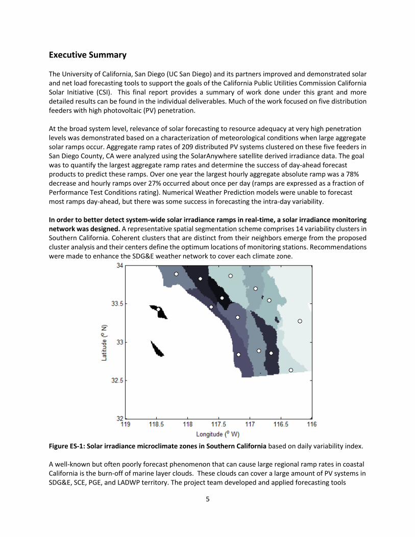
Executive Summary The University of California, San Diego (UC San Diego) and its partners improved and demonstrated solar and net load forecasting tools to support the goals of the California Public Utilities Commission California Solar Initiative (CSI). This final report provides a summary of work done under this grant and more detailed results can be found in the individual deliverables. Much of the work focused on five distribution feeders with high photovoltaic (PV) penetration. At the broad system level, relevance of solar forecasting to resource adequacy at very high penetration levels was demonstrated based on a characterization of meteorological conditions when large aggregate solar ramps occur. Aggregate ramp rates of 209 distributed PV systems clustered on these five feeders in San Diego County, CA were analyzed using the SolarAnywhere satellite derived irradiance data. The goal was to quantify the largest aggregate ramp rates and determine the success of day-ahead forecast products to predict these ramps. Over one year the largest hourly aggregate absolute ramp was a 78% decrease and hourly ramps over 27% occurred about once per day (ramps are expressed as a fraction of Performance Test Conditions rating). Numerical Weather Prediction models were unable to forecast most ramps day-ahead, but there was some success in forecasting the intra-day variability. In order to better detect system-wide solar irradiance ramps in real-time, a solar irradiance monitoring network was designed. A representative spatial segmentation scheme comprises 14 variability clusters in Southern California. Coherent clusters that are distinct from their neighbors emerge from the proposed cluster analysis and their centers define the optimum locations of monitoring stations. Recommendations were made to enhance the SDG&E weather network to cover each climate zone.

Figure ES-1: Solar irradiance microclimate zones in Southern California based on daily variability index. A well-known but often poorly forecast phenomenon that can cause large regional ramp rates in coastal California is the burn-off of marine layer clouds. These clouds can cover a large amount of PV systems in SDG&E, SCE, PGE, and LADWP territory. The project team developed and applied forecasting tools

6

consisting of very high resolution numerical weather prediction and statistical modeling. Several configurations of the Weather Research and Forecasting (WRF) model are applied to generate a distribution of forecast results for Global Horizontal Irradiance (GHI). Other models included National Weather Service forecasts and statistical models. The forecasts are validated against GHI observations from eight weather stations located along a coastal to inland gradient. The direct outputs from all numerical weather prediction models including WRF are significantly biased. Post-processing is required to improve upon simple 24 hours persistence forecasts and for the WRF models this improvement is about 30% depending on the ground station. The forecast performance is not sensitive to which input data (WRF output or past observations of GHI or both) are used. Also including additional WRF outputs aside from GHI shows little benefit. The product developed in this research could serve as an operational day-ahead marine layer solar forecast system. At the more granular level, the project focused on distribution feeder power quality analysis with total sky imager forecasts feeding into power flow modeling to identify voltage control needs. Some of the adverse impacts of high PV penetration on the power grid are an increasing number of tap operations, over-voltages, and large and frequent voltage fluctuations and PV power ramps. However, the inability to create realistic PV input profiles with high spatial and temporal resolution make the results of prior studies questionable. The project team proposes a unique method to realistically investigate these impacts and assess a feeder’s hosting capacity using (1) high resolution PV generation profiles with sky imagers (Fig. ES-2), (2) quasi-steady state distribution system simulation of the five distribution models created from data provided by a Californian utility. Solar penetration levels, defined as peak PV output divided by peak load demand, from 0% to 200%. The main conclusions were: (1) the impacts of high PV penetration depend strongly on the feeder topology and characteristics; (2) the use of a single PV generation profile overestimates the number of tap operations significantly due to an overestimation of power ramp rates and magnitudes (Fig. ES-3). Thus multiple realistic profiles should be used; and (3) a distributed allocation strategy of PV resources, rather than a centralized setup increases the feeder hosting capacity.

Fig. ES-2. A snapshot of high resolution cloud shadows over Feeder A showing more than half of the feeder area is covered by clouds, while the remaining area is clear

Fig. ES-3. Normalized tap operations of five feeders with single and multiple PV profiles configurations on a partly cloudy day relative to the tap operations at 0% penetration level. At 0% penetration feeders A, B, C, D, and E have 336, 0, 1, 13, 30 tap operations, respectively.

A control strategy to reduce tap operations (TO) resulting from high PV penetration on distribution feeders was developed and applied. The strategy uses 5 minutes ahead solar forecast to derive future

7

voltages states on the distribution feeder. Unnecessary tap operations (TO) are identified as those that are reversed within 5 minutes, likely because of temporary cloudy or clear conditions over adjacent PV systems. Unnecessary TO are eliminated (Fig. ES-4). On a feeder where TO were abundant at over 750 per day on average, the strategy resulted in the avoidance of 56% of the TO, which would result in significant savings in OLTC maintenance costs. Average extreme voltages were not affected by applying the TO reduction techniques. While daily maximum and minimum voltage excursions over the entire feeder slightly increased on several days, a statistical analysis demonstrated that these deviations happened very rarely. The strategy is most effective on partly cloudy days and on voltage regulators with a large number of TO. The fraction of avoided TO decreased substantially for less than 10 to 40 TO per day, depending on the voltage regulator. The control algorithm was shown to be robust against forecast errors inherent in state-of-the art sky imager forecasts.

Fig. ES-4. Reduction in tap operations through solar forecasting. Tap position sequences of a transformer near the end of a rural distribution feeder for three different scenarios. Originally the number of TO was 38 and tap depth was 135. Using the actual forecast those are reduced to 9 and 17. Using the perfect forecast, those are reduced to 1 and 2.

Figure ES-5: Net load forecast error versus irradiance variability. Normalized absolute net load forecast error (y-axis) for the 30 min forecast horizon versus solar irradiance step change (x-axis) for the five feeders. 𝐴𝐴𝑡𝑡 is the actual value of the load, 𝐹𝐹𝑡𝑡 is the forecast value for time 𝑡𝑡 and ∆ represents the change in GHI over these 30 min. The error is independent of the solar variability for feeders with small penetration (feeders B and C). With increasing solar penetration, the load forecast error increases linearly with solar variability.

For these same feeders net load forecast models were also developed and validated for 15 min to 5 days forecast horizons. Forecasting methods like Artificial Neural Networks optimized using Genetic Algorithms, Support Vector Regression, k-Nearest Neighbors, and various other state-space and time-series models were implemented and tested successfully. The forecasting errors were found to increase on cloudy days and to increase on feeders with higher solar penetration (Fig. ES-5). Exogenous inputs like day-ahead solar forecasts from the North American Mesoscale (NAM) NWP model were also used as an input to further refine the forecast. The accuracy of the load forecast is limited by the poor NAM forecast accuracy. Acknowledgements

8

This work was supported by the California Solar Initiative RD&D program. We are grateful to Stephan Barsun, Itron for helpful comments, guidance, and for making connections with other CSI researchers. SolarAnywhere data for all of California was provided by Clean Power Research.

9

Introduction and Key Terms Weather is a continuous, data-intensive, multidimensional, dynamic and chaotic process, and these properties make weather forecasting a formidable challenge. There is a wide range of techniques involved in weather forecasting from basic approaches to highly complex computerized models. Accurate forecasting of solar irradiance is essential for the efficient operation of solar thermal power plants, energy markets, and the widespread implementation of solar photovoltaic technology. The University of California, San Diego (UC San Diego) and its partners developed solar forecasting models and applied them in a variety of settings that support solar power integration for San Diego Gas & Electric (SDG&E) and the goals of the California Public Utilities Commission California Solar Initiative (CSI). This final report provides a summary of work done under this grant and more detailed results can be found in the individual deliverables (see reference section). Since several datasets and error metrics were used throughout different tasks, section 2 describes these data sets and equations. In particular, the SolarAnywhere satellite solar resource product, the California Solar Initiative Performance Based Incentive Program (PBI) PV power output data, and the SDG&E weather station network are described. Further, the clear sky index and bias error, absolute error, root mean square error, and forecast skill are defined. In Section 3 the solar resource throughout SDG&E territory is analyzed to study extreme distribution feeder ramp rates and recommend locations for placement of weather stations. These analyses provide insights into the seasonality and locations of large ramps on the distribution system. Further strategic input is provided on where to place irradiance sensors on the SDG&E weather station network to capture system-wide solar variability in Section 4. In Section 5, forecast models for the summertime marine layer clouds that cause large solar output ramps are presented. Numerical Weather Prediction (NWP) and statistical models are developed to forecast solar irradiance across the SDG&E territory from hours to days-ahead. In Section 6 forecasting models are applied for shorter time scales and focused on distribution feeders. Sky imagers allow the generation of detailed spatio-temporal irradiance maps over the feeder that allow the quantification of high PV penetration issues with unprecedented realism as shown in Section 7. Using sky imager forecasts, voltage regulation equipment can be operated smarter to reduce regulator actions and maintenance costs. Ultimately, solar forecasts need to be fed into net load forecasts to capture the resulting demand that needs to be supplied by the utility and conventional generators. Section 8 describes application of net load forecast models at five distribution feeders and an analysis of the impacts of solar variability on net load. Acronyms and Key Terms (see also NREL Glossary at http://rredc.nrel.gov/solar/glossary/) AC Alternating current. Typically used to characterize inverter capacity at a PV site. CMV Cloud motion vector: cloud speed and direction. DC Direct current. Typically used to characterize PV panel capacity at a PV site. DNI Direct normal irradiance GA Genetic Algorithms GFS Global Forecast System

10

GHI Global Horizontal Irradiance: sum of direct and diffuse irradiance on a horizontal surface. GOES Geostationary Operational Environmental Satellite IOU Investor-owned utilities (SDG&E, SCE, PG&E) kt Clear sky index: actual irradiance (or power output) normalized by expected clear sky irradiance or power output (Section 2.2). MAE Mean Absolute Error. MBE Mean Bias Error (Section 2.3) NAM North American Model NOAA National Oceanic and Atmospheric Administration NWP Numerical Weather Prediction PBI Performance-based incentive program: Incentive program of the CSI, where payouts are based on actual solar generation. PG&E Pacific Gas & Electric PV Photovoltaic ρ Correlation coefficient. RMSE Root Mean Square Error RR Ramp Rate SAW SolarAnywhere satellite-derived solar resource data. SCE Southern California Edison SDG&E San Diego Gas & Electric SVR Support Vector Regression SZA Solar Zenith Angle TESLA Taylor Expanded Solar Analog Forecasting ToD Time of Day UTC Universal Coordinated Timezone (PST = UTC – 8 hours). WRF Weather Research and Forecasting Model

11

Dataset and Error Metrics Data

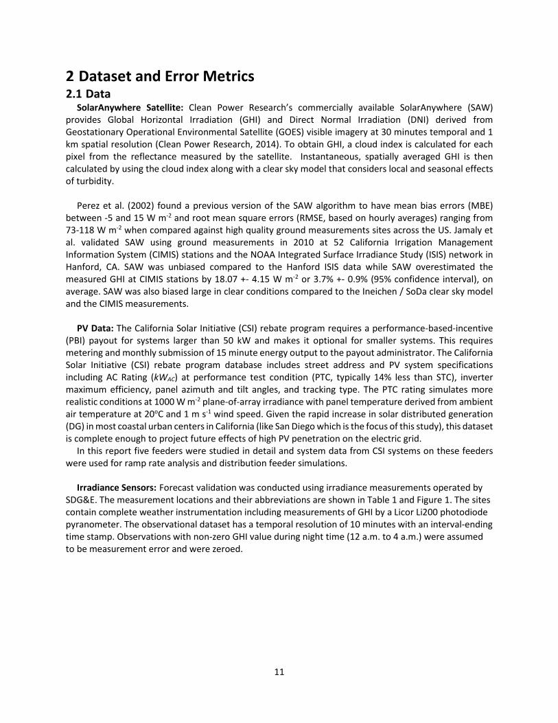
SolarAnywhere Satellite: Clean Power Research’s commercially available SolarAnywhere (SAW) provides Global Horizontal Irradiation (GHI) and Direct Normal Irradiation (DNI) derived from Geostationary Operational Environmental Satellite (GOES) visible imagery at 30 minutes temporal and 1 km spatial resolution (Clean Power Research, 2014). To obtain GHI, a cloud index is calculated for each pixel from the reflectance measured by the satellite. Instantaneous, spatially averaged GHI is then calculated by using the cloud index along with a clear sky model that considers local and seasonal effects of turbidity.

Perez et al. (2002) found a previous version of the SAW algorithm to have mean bias errors (MBE)

between -5 and 15 W m-2 and root mean square errors (RMSE, based on hourly averages) ranging from 73-118 W m-2 when compared against high quality ground measurements sites across the US. Jamaly et al. validated SAW using ground measurements in 2010 at 52 California Irrigation Management Information System (CIMIS) stations and the NOAA Integrated Surface Irradiance Study (ISIS) network in Hanford, CA. SAW was unbiased compared to the Hanford ISIS data while SAW overestimated the measured GHI at CIMIS stations by 18.07 +- 4.15 W m-2 or 3.7% +- 0.9% (95% confidence interval), on average. SAW was also biased large in clear conditions compared to the Ineichen / SoDa clear sky model and the CIMIS measurements.

PV Data: The California Solar Initiative (CSI) rebate program requires a performance-based-incentive

(PBI) payout for systems larger than 50 kW and makes it optional for smaller systems. This requires metering and monthly submission of 15 minute energy output to the payout administrator. The California Solar Initiative (CSI) rebate program database includes street address and PV system specifications including AC Rating (kWAC) at performance test condition (PTC, typically 14% less than STC), inverter maximum efficiency, panel azimuth and tilt angles, and tracking type. The PTC rating simulates more realistic conditions at 1000 W m-2 plane-of-array irradiance with panel temperature derived from ambient air temperature at 20oC and 1 m s-1 wind speed. Given the rapid increase in solar distributed generation (DG) in most coastal urban centers in California (like San Diego which is the focus of this study), this dataset is complete enough to project future effects of high PV penetration on the electric grid.

In this report five feeders were studied in detail and system data from CSI systems on these feeders were used for ramp rate analysis and distribution feeder simulations.

Irradiance Sensors: Forecast validation was conducted using irradiance measurements operated by

SDG&E. The measurement locations and their abbreviations are shown in Table 1 and Figure 1. The sites contain complete weather instrumentation including measurements of GHI by a Licor Li200 photodiode pyranometer. The observational dataset has a temporal resolution of 10 minutes with an interval-ending time stamp. Observations with non-zero GHI value during night time (12 a.m. to 4 a.m.) were assumed to be measurement error and were zeroed.

12

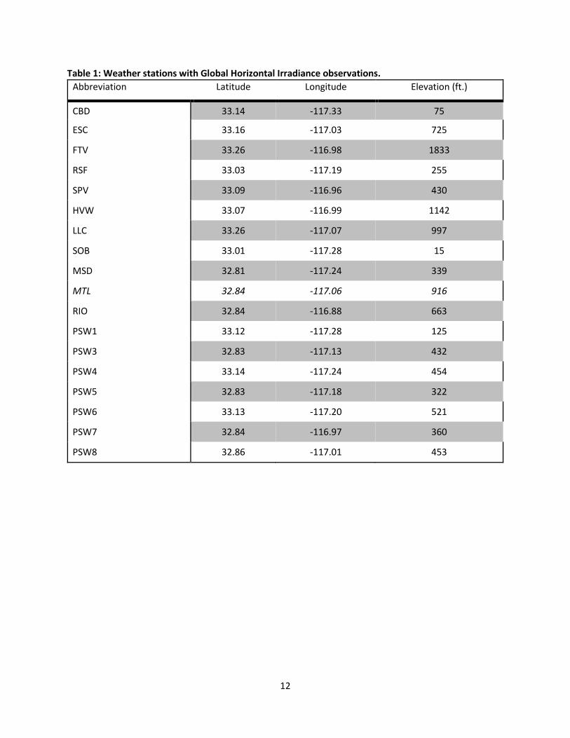
Table 1: Weather stations with Global Horizontal Irradiance observations. Abbreviation Latitude Longitude Elevation (ft.)

CBD 33.14 -117.33 75

ESC 33.16 -117.03 725

FTV 33.26 -116.98 1833

RSF 33.03 -117.19 255

SPV 33.09 -116.96 430

HVW 33.07 -116.99 1142

LLC 33.26 -117.07 997

SOB 33.01 -117.28 15

MSD 32.81 -117.24 339

MTL 32.84 -117.06 916

RIO 32.84 -116.88 663

PSW1 33.12 -117.28 125

PSW3 32.83 -117.13 432

PSW4 33.14 -117.24 454

PSW5 32.83 -117.18 322

PSW6 33.13 -117.20 521

PSW7 32.84 -116.97 360

PSW8 32.86 -117.01 453

13

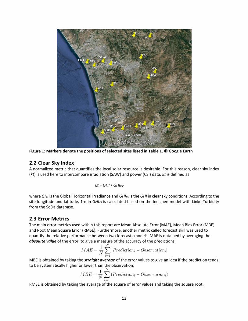
Figure 1: Markers denote the positions of selected sites listed in Table 1. © Google Earth

Clear Sky Index A normalized metric that quantifies the local solar resource is desirable. For this reason, clear sky index (kt) is used here to intercompare irradiation (SAW) and power (CSI) data. kt is defined as

kt = GHI / GHICSI where GHI is the Global Horizontal Irradiance and GHICS is the GHI in clear sky conditions. According to the site longitude and latitude, 1-min GHICS is calculated based on the Ineichen model with Linke Turbidity from the SoDa database.

Error Metrics The main error metrics used within this report are Mean Absolute Error (MAE), Mean Bias Error (MBE) and Root Mean Square Error (RMSE). Furthermore, another metric called forecast skill was used to quantify the relative performance between two forecasts models. MAE is obtained by averaging the absolute value of the error, to give a measure of the accuracy of the predictions

MBE is obtained by taking the straight average of the error values to give an idea if the prediction tends to be systematically higher or lower than the observation,

RMSE is obtained by taking the average of the square of error values and taking the square root,

14

Forecast Skill measures the performance of a forecast model with respect to a reference forecast, e.g. the performance of raw NWP or with respect to the persistence forecast. If there is no improvement, the forecast skill is 0. In the extreme case of perfect forecast, the forecast skill becomes 1.

15

Aggregate ramp Rates Analysis of Distributed PV Systems in San Diego County

Integration of large amounts of photovoltaic (PV) into the electricity grid poses technical challenges

due to the variable solar resource. Solar distributed generation (DG) is often behind the meter and consequently invisible to grid operators. The ability to understand actual variability of solar DG will allow grid operators to better accommodate the variable electricity generation for resource adequacy considerations that inform planning, scheduling, and dispatching of power. From a system operator standpoint, it is especially important to understand when aggregate power output is subject to large ramp rates. If in a future with high PV penetration all PV power systems were to strongly increase or decrease power production simultaneously, it may lead to additional cost or challenges for the system operator to ensure that sufficient flexibility and reserves are available for reliable operations.

To document actual ramp conditions, aggregate ramp rates of distributed PV systems installed in San Diego, CA and surrounding area are analyzed. Modeled irradiation data along with specifications of 209 PV systems are used to evaluate the frequency, magnitude, and ability to forecast large ramps in aggregate power output. 3.1. Data Datasets: From the 2011 CSI PBI database, specifications for 79 PV power plants on the five feeders were obtained. 130 additional sites were identified using aerial imagery in Google Earth. Site specifications were derived from the measured projected surface areas of each site by assuming a DC conversion efficiency of 15% and a DC-rating to PTC-rating ratio of 0.852. Azimuth and tilt angles were randomly selected from the specifications of nearby (same feeder) sites contained in the CSI database. Therefore, a final set of 209 PV systems with total PTC rated capacity of 4.62 MW, mean PTC rated of 22 kW, and median PTC rated of 4.7 kW are analyzed. Table 2 shows the characteristics of the different feeders. Notably on feeders A and D, the largest site (1 MW) constitutes more than half of the total capacity, which reduces geographic diversity effects. Table 2: Feeders description: Names, total PTC rating and number of sites feeding the 5 areas. The PTC rating of the largest site is shown in brackets.

Feeder name Site number Aggr PTC rating [kW] Mean Distance [km]

C 28 170 [11] 1.4

A 28 1160 [1000] 4.5

E 43 239 [13] 2.9

B 91 1151 [159] 1.3

D 19 1900 [1005] 2.6

Modeled Global Horizontal Irradiance (GHI) and Direct Normal Irradiance (DNI) are provided by Clean

Power Research’s commercially available SolarAnywhere (SAW) derived from Geostationary Operational Environmental Satellite (GOES) visible imagery (SolarAnywhere, 2011). SAW enhanced resolution satellite-

16

derived irradiation with 30-min temporal and 1 km spatial resolutions is applied in this study. At each PV system, the SAW derived GHI and DNI are used to estimate power output P by using a performance model as described in (Jamaly et al., 2012). The analysis is conducted for January 1st to December 31st, 2011. To avoid errors due to sensor cosine response and shading by nearby obstructions (not considered by SAW), only data for solar zenith angles less than 75° are considered. Performance when the solar zenith angle is less than 75º for a flat plate system is less than 26% of rated capacity so hourly ramps are likely to be substantially less during those periods.

Aggregate PV Ramp Rates: The aggregate SAW modeled power output for each area of study is used

to determine the largest absolute ramp rates in 2011. From the aggregate PV power output at each time step, differences are calculated for different ramp duration intervals; 30-min through 5-hour in 30-min increments.

We present normalized absolute ramp rates to facilitate scaling the results to future PV penetration scenarios (assuming a similar geographic diversity). Therefore, the aggregate power outputs are normalized by the aggregate (PTC) kWAC capacity of the PV systems for each area.

Day ahead forecast: In addition, day-ahead forecasts of the PV power production have been calculated

for each of the 209 sites. A high-resolution (1.3 km), direct-cloud-assimilating Numerical Weather Prediction (NWP) model based on the Weather and Research Forecasting model (WRF) forecasts instantaneous hourly GHI day ahead (Mathiesen et al. 2013). Satellite observations of cloud cover at model initialization are assimilated into the model. Forecasts with (WRFA) and without (WRF) cloud assimilation have been calculated for May and June 2011 when the marine layer cloud events are more frequent in the coastal areas. These forecasts have been used to determine the next day expected power output variability and compared with the measured variability.

3.2. Daily Variability Index

Following a method developed at UC San Diego and Sandia National Labs (Stein et al. 2012), the daily variability is calculated for each day in terms of a Variability Index (VI). The VI was modified to allow the use of aggregated PV power output (rather than irradiance):

VI =∑day |RR|

∑day |RRclear|,

where the absolute values of the 1-hour ramp rates (RR) are summed and divided by the sum of the absolute 1-hour ramp rates that would have occurred if the day was clear (RRclear). This index will be 1 for a clear day and larger than 1 for days with partial cloud cover. It can also take values below 1 for overcast days. 3.3. The Largest Ramps

3.3.1. Largest Ramp Rates by Time Horizon

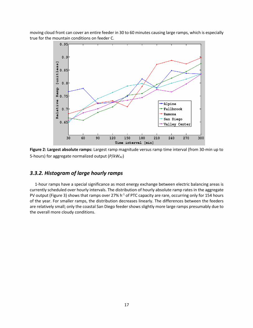
The largest step sizes in the absolute aggregate PV power output (normalized by kWAC) are detected over the year for different intervals (Figure 2). As expected, the maximum ramp magnitude increases with the ramp interval approaching 90% for 5 hour ramps reflective of the diurnal cycle (e.g. from zero output at 0700 to near maximum output at 1200 solar time) on a clear day. However, the ramp magnitudes are already at 65 to 77% over 30 minutes, which is much larger than the SDG&E-wide ramps observed in [Jamaly et al., 2012, 2013]. The reason is the relatively small geographic diversity within a feeder. A fast-

17

moving cloud front can cover an entire feeder in 30 to 60 minutes causing large ramps, which is especially true for the mountain conditions on feeder C.

Figure 2: Largest absolute ramps: Largest ramp magnitude versus ramp time interval (from 30-min up to 5-hours) for aggregate normalized output (P/kWAC)

3.3.2. Histogram of large hourly ramps

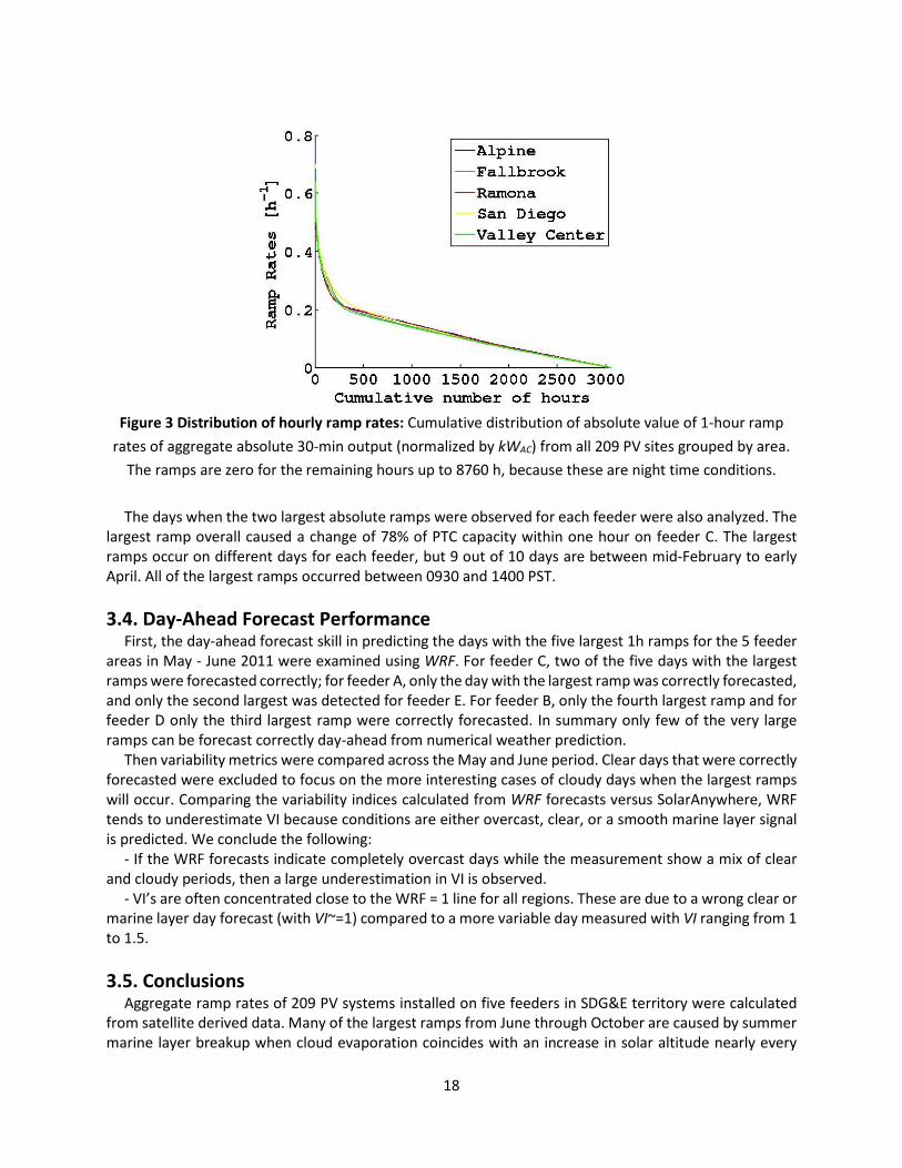
1-hour ramps have a special significance as most energy exchange between electric balancing areas is currently scheduled over hourly intervals. The distribution of hourly absolute ramp rates in the aggregate PV output (Figure 3) shows that ramps over 27% h-1 of PTC capacity are rare, occurring only for 154 hours of the year. For smaller ramps, the distribution decreases linearly. The differences between the feeders are relatively small; only the coastal San Diego feeder shows slightly more large ramps presumably due to the overall more cloudy conditions.

18

Figure 3 Distribution of hourly ramp rates: Cumulative distribution of absolute value of 1-hour ramp

rates of aggregate absolute 30-min output (normalized by kWAC) from all 209 PV sites grouped by area. The ramps are zero for the remaining hours up to 8760 h, because these are night time conditions.

The days when the two largest absolute ramps were observed for each feeder were also analyzed. The

largest ramp overall caused a change of 78% of PTC capacity within one hour on feeder C. The largest ramps occur on different days for each feeder, but 9 out of 10 days are between mid-February to early April. All of the largest ramps occurred between 0930 and 1400 PST.

3.4. Day-Ahead Forecast Performance

First, the day-ahead forecast skill in predicting the days with the five largest 1h ramps for the 5 feeder areas in May - June 2011 were examined using WRF. For feeder C, two of the five days with the largest ramps were forecasted correctly; for feeder A, only the day with the largest ramp was correctly forecasted, and only the second largest was detected for feeder E. For feeder B, only the fourth largest ramp and for feeder D only the third largest ramp were correctly forecasted. In summary only few of the very large ramps can be forecast correctly day-ahead from numerical weather prediction.

Then variability metrics were compared across the May and June period. Clear days that were correctly forecasted were excluded to focus on the more interesting cases of cloudy days when the largest ramps will occur. Comparing the variability indices calculated from WRF forecasts versus SolarAnywhere, WRF tends to underestimate VI because conditions are either overcast, clear, or a smooth marine layer signal is predicted. We conclude the following:

- If the WRF forecasts indicate completely overcast days while the measurement show a mix of clear and cloudy periods, then a large underestimation in VI is observed.

- VI’s are often concentrated close to the WRF = 1 line for all regions. These are due to a wrong clear or marine layer day forecast (with VI~=1) compared to a more variable day measured with VI ranging from 1 to 1.5.

3.5. Conclusions

Aggregate ramp rates of 209 PV systems installed on five feeders in SDG&E territory were calculated from satellite derived data. Many of the largest ramps from June through October are caused by summer marine layer breakup when cloud evaporation coincides with an increase in solar altitude nearly every

19

morning. During the winter months, the ramp rates are mainly caused by winter frontal storm systems; when fast-moving storm systems move into the area (creating a large down ramp) or out of the area (creating a large up-ramp).

This analysis was focused on distributed PV generators less geographically diverse than those analyzed in previous reports. As expected this resulted in larger ramps (with a maximum of 78% per 30 minutes) than those observed for PV systems that were relatively well distributed across the SDG&E service area (with a maximum of 44% per 30 minutes).

Day ahead power output forecasts from high-resolution Numerical Weather Prediction model did not show significant skill in forecasting large ramps, even statistically. Further research is required to improve NWP forecasts.

20

Recommended Placement of SDG&E Weather Stations to Capture Solar Variability and Improve Forecast Skill

4.1. Data and Methodology To optimize the deployment of GHI sensors in the SDG&E territory a method was developed to separate distinct climate zones based on satellite solar resource data. Existing irradiance sensors and weather stations owned by SDG&E were identified. Remote sensing data from SolarAnywhere in 2009 and 2010 (v2.0, see Section 2) was used to estimate irradiance variability and the presence of specific solar microclimates within the SDG&E service territory. Two variability metrics were studied: Variability Metric #1 The daily average clearness over each location of the gridded domain was extracted from the normalized GHI data. Variability Metric #2 Additionally, a second variability metric was added in order to emphasize daily fluctuations of the clearness index. The variability index is described by the consecutive absolute step changes of the daily average clear sky index over a precise surface area (see Section 3.2). 4.2. Recommendations for Station Placement Depending on the used variability metric, a representative spatial segmentation scheme comprises 16 (variability metric #1) or 14 (variability metric #2) variability clusters in Southern California. Respectively, 8 and 7 of them are located in the SDG&E service area. Coherent clusters that are distinct from their neighbors emerge from the proposed cluster analysis and their centers define the optimum locations of monitoring stations. Here only results for variability metric #2 are presented in Figure 5.

21

Figure 4: 14 identified irradiance microclimate clusters with cluster centers in Southern California. Relevant relationships between locations are summarized in Table 3 and Figure 6 for the seven identified clusters and closest SDG&E met station and closest SDG&E met station with GHI sensors are listed. All cluster centers have a SDG&E weather station with GHI sensor within 4.1 miles. We recommend placement of sensors at location TDS (1), MPE (4) and FBK (5). The data acquisition frequency should be set to once every 30 seconds or faster to resolve fast solar ramps.

Table 3: Results based on variability metric #2, the day-to-day variation in averaged clear sky index (see Fig. 6 for a map). 7 cluster centers are identified. The closest SDG&E met station is listed and (GHI) indicates that that station already has a global horizontal solar irradiance (GHI) sensor.

Location of Cluster Center

Closest SDG&E Met Station Distance and direction to SDGE station. Station is

1 32.633 -116.331 TDS BVDC1 (GHI)

1.2 miles 4 miles

2 32.854 -116.652 WDC NDC (GHI)

1.3 miles 2 miles

3 32.884 -116.853 BVY RIO (GHI)

1.3 miles 3.2 miles

22

4 32.834 -117.174 MPE MSP (GHI)

3.5 miles 4.1 miles

5 33.327 -117.194 FBK CIR (GHI)

2.5 miles 4 miles

6 33.578 -117.445 ORT (GHI) 3.8 miles

7 33.457 -117.615 SCR (GHI) 2.1 miles

Figure 5: Irradiance microclimate clusters in the SDG&E service area, based on variability metric #2 (7 cluster centers).

23

Day-Ahead Solar Forecast Models for Marine Layer Clouds Numerical weather prediction (NWP) is generally the most accurate tool for forecasting solar irradiation several hours in advance (Mathiesen et al., 2011). These methods model the weather numerically and use time integration to forecast the future state of the weather and solar irradiance. Despite computational complexity and intensity, the multitude of parameterizations employed and insufficient grid resolution cause the direct output from these models to be inaccurate. Machine learning techniques, on the other hand, assume that the complex physical relationships can be mapped to simpler functional relationships between the key variables at much smaller computational cost. One family of methods is the analog method family. It hypothesizes that what will happen tomorrow has already happened in the past. Considering past observations and forecasts, called the ensemble set, analog forecasts predict which date or dates are most similar (“analogous”) to the forecast period. Analog methods can be either used for post-processing of a numerical weather model output or for forecasting directly from historical measurements. Post-processing is the process of taking forecast products of another tool and improving them. This section describes a new analog based forecasting algorithm called Taylor Expanded Solar Analog Forecasting (TESLA) applied to observations and NWP output from coastal California. In southern California, low-altitude marine layer stratocumulus cloud (MLS) cover is common during April through September mornings. Generally these clouds are optically thick and can reduce solar photovoltaic production by up to 70%. The primary objective is to forecast the burn-off of marine layer clouds. 5.1. Post-Processing Methodology Our analog method uses past observations and NWP forecasts as input parameters to calculate Global Horizontal Irradiance (GHI) forecasts. The past observation and NWP forecast set is called the ensemble set. Simply put, TESLA provides a numeric function that transforms the ensemble set into a prediction. The input parameters can be the observations from 24 hours ago or the predictions of an NWP, or virtually anything that may or may not seem relevant to the prediction. TESLA uses the ensemble set to "learn/train" how the past inputs are related to the past actual observations and produce the function that maps this connection between the inputs and the prediction. This learning process automatically filters out irrelevant inputs and adjusts the weights of the relevant inputs to produce the function that minimizes the error in the past ensemble set. More detailed analysis on how TESLA is implemented and the configurations applied are provided in the Task report. TESLA uses the ensemble database to train its prediction function(s). As the size of this ensemble set increases, the prediction quality also increases. Conversely, there also exists a minimum ensemble set size that depends on the other configuration parameters, below which the quality will drop significantly. For the TESLA configuration applied in this report, the minimum training set size was found to be 60 days, on average. 5.2. Observations and Forecast Data

5.2.1. Overview of Forecast Models

NWP forecast models include:

24

• GFS: Global Forecast System. Clear sky index interpolation was applied to generate a dataset with 15 min time steps.

• NAM: North American Mesoscale Model. Clear sky index interpolation was applied to generate a dataset with 15 min time steps.

• Green Power Labs (GPL) model. This is the probabilistic model developed under Task 3.1 of the same CSI contract and is described in more detail in a separate report by GPL1. The version of the probabilistic model applied here was an operational version during mid-phase of the project and is different from the final version applied in the GPL report (see “New Probabilistic” in the GPL report). The GPL report also uses a different geographic area and time period for validation and therefore the results are not directly comparable.

• National Weather Service (NWS) post-processed NAM from the National Digital Forecast Database (NDFD)

• 24 hour persistence forecast • UCSD post-processed Weather Research and Forecasting (WRF) model. Five different WRF

model configurations were run as detailed in the following section.

5.2.2. WRF: Weather Research and Forecasting

The WRF model is a state-of-the-art NWP and atmospheric simulation system that is maintained and supported as a community model (Skamarock et al., 2008). In this work, the version WRF V3.5 was used and configured with two nests of horizontal resolutions of 12.5 km and 2.5 km (Figure 7). The NAM, initialized at 12 UTC was used to derive boundary conditions for the outer domain. The WRF simulations were initialized at 0 UTC and run for 36 hours with 12 hours as spin-up time. The base WRF configuration, denoted as Base WRF (WRF without cloud data assimilation), is summarized in Table 4.

Figure 6: WRF simulation domains showing a nesting from a large domain with a spacing of Δx = 12.5 km to a small domain with a spacing of 2.5 km.

1 http://www.calsolarresearch.org/images/stories/documents/Sol3_funded_proj_docs/UCSD/ML-ProjRpt-CPUC_UCSD_2014-05-30.pdf

25

Table 4: Summary of the main WRF configuration. For details refer to the WRF user guide. Domain/Time Options for Inner Domain

Physics Options (WRF Option #)

Δx (km) 2.5 Cumulus NSAS (14)

Vertical Pts. 75 Radiation New Goddard (5)

Output Interval (min) 15 Microphysics Morrison (10)

Spin-Up (hr) 12 PBL MYNN (5)

Initial & boundary conditions 12 UTC NAM LSM RUC (3)

Due to the difficulty of simulating marine layer stratocumulus, one configuration of WRF physics options is not able to consistently produce accurate forecast. Therefore, ensemble forecasts are created by running multiple forecasts, each with a unique variation in the configuration to represent the different sources of uncertainty. López-Coto et al., (2014) demonstrated that the cumulus scheme is the most important parameterization generating variability in simulating marine stratocumulus in coastal southern California. The second important parameterization is the radiation scheme. In addition, when the NSAS cumulus scheme was used, the microphysics option had a strong influence. In addition to the model physics, the initial conditions were also varied. Mathiesen et al. (2013) developed the WRF-Cloud Data Assimilation (CLDDA) using Geostationary Operational Environmental Satellite (GOES) imagery to directly assimilate clouds in the initial conditions. Validated using the UCSD pyranometer network, the WRF-CLDDA was shown to be 17.4% less biased than the NAM. Therefore, in addition to the base case listed in Table 4 , four WRF simulations were conducted using three cumulus, two radiation and two microphysics schemes. Table 5 showing the unique variations of each scheme relative to the base case. Table 5: Summary of unique configurations for four different WRF ensembles

Ensemble Name Cumulus Radiation Microphysics

Cumulus1 Kain-Fritsch (1) Dudhia (1) / RRTM (1)

Microphysics8 Thompson (8)

CLDDA

CLDDA& Cumulus 3 Grell-Freitas (GF) (3)

5.3. Raw Forecast Performance The results of the raw (no postprocessing) forecast model output for the May – September marine layer forecast trials were compiled in Figure 8 and Figure 9. The NOAA models (NAM and GFS) have severe deficiencies in forecasting marine layer cloud cover; even for the coastal sites, most forecasts are clear. The National Weather Service (NDFD) post-processing correctly predicts morning clouds, but misses days that are completely overcast. The performance of the GPL model is the worst of any of the custom models with a hit rate on par with NAM and GFS. Persistence forecast and UCSD WRF configurations that include cloud data assimilation from satellite images (wrfcldda) perform best. In the San Diego summer climate, the absence of frontal passage causes significant ‘inertia’ in the weather conditions.

26

Weather conditions change typically over time periods of 2-5 days and therefore a 24-hour persistence forecast is very accurate and difficult to beat.

Figure 7: Hit score = 0.5 (Cloudy hit [%] + Clear hit [%]) for the forecast models averaged over CBD, ESC,

PWS1, PWS4, PWS5, PWS7 and PWS8 sites. The results at other stations are qualitatively similar.

Figure 8: Daytime mean absolute error for the different weather forecast

27

5.4. Post-processed forecast performance

5.4.1 Forecast Bias

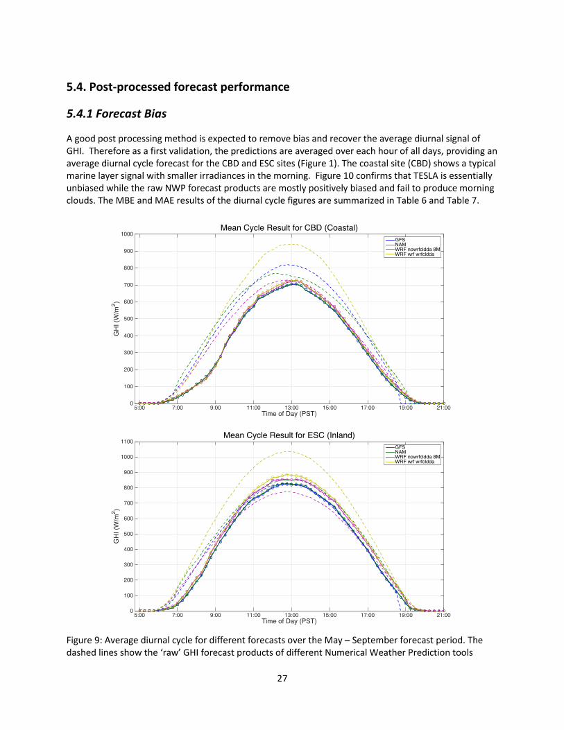
A good post processing method is expected to remove bias and recover the average diurnal signal of GHI. Therefore as a first validation, the predictions are averaged over each hour of all days, providing an average diurnal cycle forecast for the CBD and ESC sites (Figure 1). The coastal site (CBD) shows a typical marine layer signal with smaller irradiances in the morning. Figure 10 confirms that TESLA is essentially unbiased while the raw NWP forecast products are mostly positively biased and fail to produce morning clouds. The MBE and MAE results of the diurnal cycle figures are summarized in Table 6 and Table 7.

Figure 9: Average diurnal cycle for different forecasts over the May – September forecast period. The dashed lines show the ‘raw’ GHI forecast products of different Numerical Weather Prediction tools

28

without post-processing. The solid lines show the TESLA Order 2 predictions using the GHI output of the forecast products. The circles show the observations. A) Coastal station CBD. (B) Inland station ESC. Table 6: Error Statistics for the CBD Coastal Station in W m-2.

CLDDA&Cumulus3

CLDDA Microphysics8

Cumulus Base WRF NAM GFS

MAE Tesla

1.53 0.79 1.59 0.82 1.11 0.90 0.95

MAE Raw

54.00 85.70 24.40 89.23 82.43 58.25 61.32

MBE Tesla

-1.52 -0.60 -1.59 -0.58 -0.97 -0.85 -0.89

MBE Raw

53.90 85.58 23.30 88.60 82.30 57.44 58.57

Table 7: Error Statistics for the ESC Inland Station in W m-2.

CLDDA&Cumulus

3

CLDDA Microphysics8

Cumulus Base WRF NAM GFS

MAE Tesla

0.92 0.78 0.59 1.36 0.54 0.48 0.56

MAE Raw

66.11 65.77 31.72 47.05 45.46 31.7 16.84

5.4.2 Forecast RMSE: Choice of TESLA Configuration

TESLA forecast results for 120 days were analyzed. TESLA methods include Order 1 and Order 2 Taylor series expansions applied to the ensemble set with past observations and NWP GHI. Since the order has little impact on forecast error, Order 2 is used from here on out. 15 minute prediction functions are used, i.e. a separate function is fit to all 96 forecast intervals during the day. Nighttime prediction functions could be eliminated to reduce the computational cost, but are included with the error metrics. Sensitivity to type of input variables: TESLA is applied (i) using no input (i.e. only a bias correction is performed), (ii) using NWP GHI only, (iii) past observations only, and (iv) using observations and NWP GHI as inputs. Table 8 shows the overall forecast skill and Figure 11 shows an example by station. The forecast results are not strongly sensitive to the type of input variables. As expected, a bias correction (no input) performs worst and providing NWP and observation data results in the best forecast performance. However, the relatively persistent weather conditions in coastal California in the summer cause simple bias corrections to be quite effective. This performance difference may not be enough compared to the effort and time required to generate the WRF forecasts.

29

Table 8: Overall forecast results as a function of different input parameters and TESLA configurations. The forecast skill is measured with respect to the raw NWP forecast for various cases. A larger forecast skill is better.

Overall Forecast Skill [1-RMSE(TESLA)/RMSE(NWP)] Input Type None NWP GHI Only Past

Observations Only

NWP GHI and Past Observations

TESLA Order 2 Func./15 Minute

0.44 0.47 0.48 0.48

TESLA Order 1 Func./15 Minute

0.44 0.45 0.47 0.48

Input Parameters (See Figure 12)

[1] [2] [3] [4] [5] [6] [7]

TESLA Order 2 Func./15 Minute

-12.36 -0.86 0.36 0.37 0.03 0.38 0.34

TESLA Order 1 Func./15 Minute

0.00 0.36 0.36 0.37 0.35 0.36 0.36

TESLA Order 2 Func./1 Day

-2.03 0.18 0.22 0.21 0.21 0.23 0.20

TESLA Order 1 Func./1 Day

0.32 0.34 0.33 0.34 0.33 0.33 0.32

Figure 10: Marine layer solar forecast RMSE results with TESLA Order 2 using different NWP GHI outputs and past observations as input parameters. Sensitivity to NWP input variables: In this section, we compare the effect of using different input parameters from NWP on the prediction quality. For this analysis the base WRF configuration is used and TESLA output is compared against measurements at CBD.

30

Figure 11: Marine layer solar forecast RMSE results with TESLA Orders 1 and 2 using different WRF output variables and past observations as input: [1] – All variables, [2] – GHI, Columnar Cloud Cover,

Surface Pressure, Height 850 & 700, [3] – GHI and Height 700, [4] – GHI and Surface Pressure, [5] – GHI and Columnar Cloud Cover, [6] – GHI Only, [7] –Temperature at Surface, 850 & 700 mbar.

We can see that when all WRF variables are used to train the TESLA prediction function, large errors result, since the training dataset size requirement increases exponentially with increasing number of parameters. From the rest of the variable combinations, we conclude that a single WRF output - GHI – results in the smallest error. Using a single variable is also the simplest to implement operationally. If the best result for every site is selected over all possible input parameters and forecast tools, the results in Figure 13 are obtained. The improvement over 24 hour persistence ranges from 23% to 39%.

Figure 12: Forecast skill with respect to a 24 hour persistence forecast by the best performing TESLA implementation for every site, selected over all possible input parameters and forecast tools.

31

5.5. Conclusions The direct outputs from any numerical weather prediction model including WRF are significantly biased. Postprocessing is required to improve upon simple 24 hours persistence forecasts and for the WRF models this improvement is about 30% depending on the ground station. A postprocessing implementation that derives a different prediction function every 15 minutes and uses a second order algorithm delivers the best performance. The forecast performance is not sensitive to which input data (WRF output or past observations of GHI or both) are used. Also including additional WRF outputs aside from GHI shows little benefit. The resulting forecast model is relatively easy to implement. Generating WRF forecasts is computationally expensive, but the postprocessing can be conducted quickly on a personal computer. In the future, the forecasts will be implemented operationally on SDG&E computers. System-wide fleet and local feeder forecasts will present an opportunity for improved local voltage control and managing system-wide ancillary services to reduce operating costs and facilitate solar power integration.

32

Localized Solar Forecasting for Distribution Feeder Modeling Sky Imager Forecasting Algorithm Development

Through cost share from the National Renewable Energy Laboratory (NREL), the University of California, San Diego (UCSD) has developed a forecasting methodology which uses ground-based sky imaging hardware. The benefit of using sky imager observations over a large ground sensor network is that only a few instruments deployed around the area of interest are capable of determining the current distribution and movement of cloud cover at a high resolution. Future cloud configurations can then be forecast at high spatial and temporal resolutions within the 0-30 minute forecast window. In contrast, a sensor array designed for forecasting may have prohibitive capital and maintenance costs. The network must be configured with sufficiently dense spacing in the entire surrounding area so that there is a lead time in the direction of cloud motion. This is not feasible in most situations from both a land use and cost perspective. This report describes UCSD’s deterministic sky imager forecast approach applied to a 48 MW section of Sempra US Gas & Power’s Copper Mountain solar power plant.

6.1.1. Experimental Setup and Data

Two Total Sky Imagers (Yankee Environmental Systems Inc., TSIs) were installed at Sempra US Gas and Power’s Copper Mountain Solar 1 power plant to validate the sky imager forecast methodology in a utility-scale environment (Figure 14). The cadmium telluride thin film panels cover approximately 1.3 km2 and are connecte to 96 inverters. The TSIs were spaced 1.8 km apart using the configuration shown in Figure 14. Fifteen calibrated reference cells provided plane-of-array global irradiance (GI) at 1 sec and five weather stations provided standard meteorological measurements including plane-of-array GI and GHI from Kipp & Zonen CMP11 broadband pyranometers. The sky imagers were installed on June 17, 2011. Several initial problems were present with data transfer, sky imager cleaning, and misalignment of the shadowband. High quality imagery has been acquired near continuously since August 5, 2011. The imagery is streamed in real-time to the CAISO renewables desk. All inverter power output, reference cell, and pyranometer data have also been archived.

33

Figure 13 Copper Mountain Power Plant: Outline of the 48MW section of the Sempra US Gas and

Power Copper Mountain Solar power plant, with sky imager locations indicated. Each inverter's panel footprint is shaded with a different gray level.

6.1.2. Cloud Forecast Methodology

The method used to generate sky imager forecasts for the Copper Mountain case study follows that of Chow et al. (2011). The forecast procedure is outlined in the flow chart in Figure 15. The procedure is broken up into two steps - one that relies on sky imager data and one that is designed for the power plant being studied. A brief explanation of the procedure is contained within this section.

Sky imager used to generated current forecastsSky imager used for cloud height

1.8 km

34

Figure 14: Sky imager forecast procedure: Flow chart showing the basic operations for constructing the power forecast in the Copper Mountain case study.

After a new image is collected, image specific masks (for the sun, shadowband, etc), and a calibration map of scattering angle based on the current solar zenith angle are constructed for the entire image. Following this, clouds are detected and cloud altitude is computed. The binary cloud/no cloud information is still in the original image coordinates, but what is needed is a georeferenced mapping of the clouds. To obtain this, a pseudo-cartesian transform maps cloud information to a latitude-longitude grid at the cloud altitude. This transform requires imaging system calibration such that each pixel has a known look angle (zenith and azimuth coordinate pair), i.e. the spherical coordinates without the radial dimension. The resulting georeferenced map of clouds is termed the 'cloudmap', which is a planar mapping of cloud position at a specified altitude above the forecast site. Of the two TSIs installed at the plant, only the northwestern unit was used in this case study to generate cloudmaps for forecasting. The second unit provided the cloud height only.

The cloud velocity is then used to advect the planar cloudmap to generate a cloud position forecast for

each forecast interval. The cloud position every 30 s is computed out to a 15 min forecast horizon for every new image captured. The forecast domain is defined by a grid overlaying the plant that is 4×4 km in size with a resolution of 2.5 m per forecast cell (1600×1600 cells), and each cell is resolved to a latitude, longitude, and altitude (the latter is obtained from a digital elevation model). For each forecast cell, a ray is traced along the vector to the sun and the intersection with the cloudmap is determined. If the intersected point is clear, that ground location is deemed clear, whereas if the intersection is cloudy, the ground point is deemed shaded by cloud. Repeating the shadow mapping process for each forecast cell constructs a map of cloud shadows (shadowmap). This shadowmap provides the percentage of the plant that is shaded. Shadowmaps are constructed for each advected cloudmap out to the 15 minute forecast horizon (generating 30 forecasted shadowmaps). The method to generate power output from the binary set of shadowmaps is site specific and described in the next section.

Calibrate Image

Compute RBR

Cloud Detection

CSL Construction

Cloud Height

Cloud Velocity

Pseudo-Cartesian Transform

Cloud Advection

Shadowmapping

New Image

New Power Data

Normalize Power

Clear sky model

Construct Probability Distribution

Clear & cloudy mode detection

Power output

Sky Imager Power Plant

35

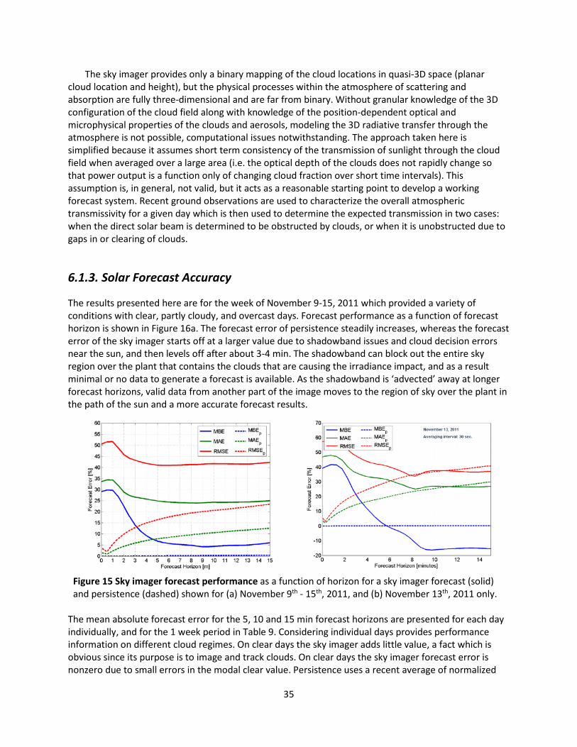
The sky imager provides only a binary mapping of the cloud locations in quasi-3D space (planar cloud location and height), but the physical processes within the atmosphere of scattering and absorption are fully three-dimensional and are far from binary. Without granular knowledge of the 3D configuration of the cloud field along with knowledge of the position-dependent optical and microphysical properties of the clouds and aerosols, modeling the 3D radiative transfer through the atmosphere is not possible, computational issues notwithstanding. The approach taken here is simplified because it assumes short term consistency of the transmission of sunlight through the cloud field when averaged over a large area (i.e. the optical depth of the clouds does not rapidly change so that power output is a function only of changing cloud fraction over short time intervals). This assumption is, in general, not valid, but it acts as a reasonable starting point to develop a working forecast system. Recent ground observations are used to characterize the overall atmospheric transmissivity for a given day which is then used to determine the expected transmission in two cases: when the direct solar beam is determined to be obstructed by clouds, or when it is unobstructed due to gaps in or clearing of clouds.

6.1.3. Solar Forecast Accuracy

The results presented here are for the week of November 9-15, 2011 which provided a variety of conditions with clear, partly cloudy, and overcast days. Forecast performance as a function of forecast horizon is shown in Figure 16a. The forecast error of persistence steadily increases, whereas the forecast error of the sky imager starts off at a larger value due to shadowband issues and cloud decision errors near the sun, and then levels off after about 3-4 min. The shadowband can block out the entire sky region over the plant that contains the clouds that are causing the irradiance impact, and as a result minimal or no data to generate a forecast is available. As the shadowband is ‘advected’ away at longer forecast horizons, valid data from another part of the image moves to the region of sky over the plant in the path of the sun and a more accurate forecast results.

Figure 15 Sky imager forecast performance as a function of horizon for a sky imager forecast (solid) and persistence (dashed) shown for (a) November 9th - 15th, 2011, and (b) November 13th, 2011 only.

The mean absolute forecast error for the 5, 10 and 15 min forecast horizons are presented for each day individually, and for the 1 week period in Table 9. Considering individual days provides performance information on different cloud regimes. On clear days the sky imager adds little value, a fact which is obvious since its purpose is to image and track clouds. On clear days the sky imager forecast error is nonzero due to small errors in the modal clear value. Persistence uses a recent average of normalized

36

power which is more accurate than the most frequent daily value (i.e. the mode) when the input solar signal is not impacted by clouds. The storm on November 11 brought very optically thick clouds which caused an error in the cloud decision step erroneously yielding clear sky forecasts. This issue has been addressed in new cloud decision research (Ghonima et al., 2012). As a result of the poor cloud decision, the forecast error was very large on this day. When there are clouds, the sky imager adds value because it can forecast when a ramp will occur, and it can provide a reasonable approximation of the magnitude. Partly cloudy days with significant ramping occurred on the 10, 12, and 13. The error on the 13 is shown as a function or forecast horizon in Figure 16b. Due to frequent ramping, the persistence forecast error increases significantly after a few minutes, and the sky imager performs better using the gross statistics.

Table 9 Sky imager and persistence forecast error at selected time horizons of 5, 10 and 15 minutes. Error is given as mean absolute error. Error is reported for individual days and the aggregate set of days as a percentage of average power generated during daylight hours. The c superscript indicates the day was clear. 5 min. 10 min. 15 min. SI P SI P SI P

9c 4.5 0.9 5 1.3 5.1 1.7 10 42.6 14.9 39 18.5 42 22.1 11 152.7 8 161.8 13.9 157.7 18.6 12 33.9 23.2 33.6 30.7 38.8 35.6 13 32 17.5 26.5 24.7 26.4 29.3

14c 4.9 1.5 4.2 1.9 4.1 2.2 15c 6.7 1.3 6.7 1.8 6.7 2

1 week 24.9 7.8 24.3 10.6 25 12.6

The ability for a sky imager to capture ramps is illustrated in Figure 17 for the 10 minute forecast horizon. Constant values in the sky imager forecast indicate periods when the plant is forecast to be entirely clear or entirely cloudy. The offset in the magnitude of the "constant value periods" is due to the histogram method of constructing power output and is expected given the method's simplicity and assumptions. Temporal shifting of ramp forecasts versus actual ramps can be seen, in both the early or late directions. Ramps are also missed and falsely predicted. The ramp forecast is directly related to how well the shadows predicted by the sky imager match plant observations. Ramp timing errors are caused by any combination of inaccurate cloud decision, camera resolution, geometric calibration errors, cloud advection errors, and differences in cloud morphology due to viewing angle. Because of the novelty of the system, each error source described can be improved markedly and thus the overall ramp forecast performance is expected to improve.

37

Figure 16 Sample Sky Imager Forecast: Midday 10 minute forecast performance on November 13th, 2011 showing how the sky imager captures ramps at 10 minutes in the future. A perfect forecast would have both curves matching exactly.

6.1.4. Discussion and Conclusions

The performance results for the selected week indicate that more work is required to make sky imagery based short-term forecasting a viable technique. The key finding in this study is that the TSI as an instrument is not suitable for generating short-term solar power forecasts. The reasons for this are: a) the shadowband eliminates important sky data for forecasting and its presence makes assessment of forecast errors due to geometry more challenging (i.e. it makes research on forecast improvement more difficult); b) low resolution imagery that is jpg compressed, further reducing information content, c) cloud decision errors near the sun and the horizon. The partly cloudy days should be considered as true indicators of how the current forecast methods perform. These three days (10, 12, and 13) provide the most representative accounting for the current status of the sky imager forecasts. Many of the errors here beyond the 5 minute forecast horizon (which is plagued by the shadowband) are attributable to geometric errors in the pseudo-cartesian transformation. The causes are both the geometric calibration of the instrument, and the flat cloud field assumption. Higher accuracy geometric calibration procedures are being applied to new instrumentation, and new algorithm development is underway to move from the 2D cloud field assumption, to construction of the cloud field in 3D. As mentioned, the MBE, MAE, and RMSE are truly gross statistics and do not fully characterize all aspects of forecast performance. These metrics indicate that, overall, persistence performs much better than the sky imager. When interpreting the performance results provided by the metrics in equations (5),(6) and (7) it is important to remember that they do not capture the ability of the system to capture ramp events. These metrics measure only the typical difference between the forecasts and the actual power produced. For instance, during a clear period persistence will provide a smaller forecast errors than the algorithm presented, but it will never predict a ramp from an oncoming cloud. To eliminate shadowband and resolution issues, the Kleissl group has built an advanced sky imager (named USI) that was deployed in the CSI4 project at San Diego distribution feeders.

38

6.2. Sky Imager Solar Forecasting at Three Distribution Feeders

6.2.1. Sky imager setup and operation

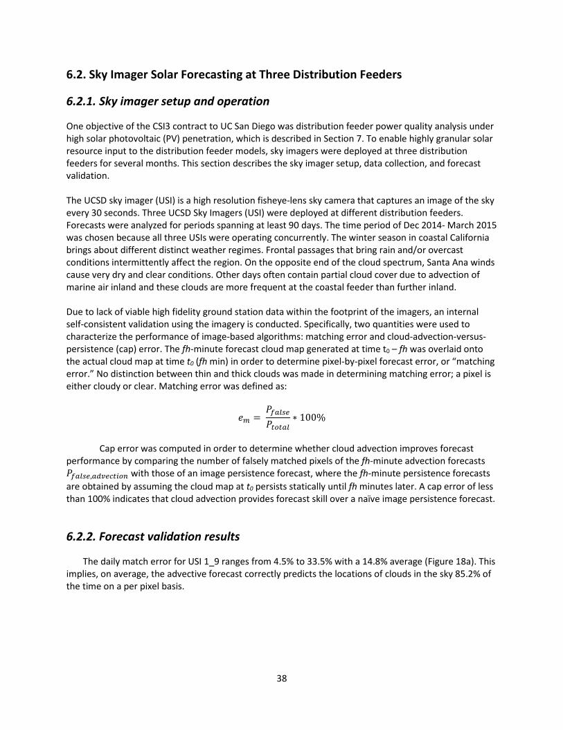
One objective of the CSI3 contract to UC San Diego was distribution feeder power quality analysis under high solar photovoltaic (PV) penetration, which is described in Section 7. To enable highly granular solar resource input to the distribution feeder models, sky imagers were deployed at three distribution feeders for several months. This section describes the sky imager setup, data collection, and forecast validation. The UCSD sky imager (USI) is a high resolution fisheye-lens sky camera that captures an image of the sky every 30 seconds. Three UCSD Sky Imagers (USI) were deployed at different distribution feeders. Forecasts were analyzed for periods spanning at least 90 days. The time period of Dec 2014- March 2015 was chosen because all three USIs were operating concurrently. The winter season in coastal California brings about different distinct weather regimes. Frontal passages that bring rain and/or overcast conditions intermittently affect the region. On the opposite end of the cloud spectrum, Santa Ana winds cause very dry and clear conditions. Other days often contain partial cloud cover due to advection of marine air inland and these clouds are more frequent at the coastal feeder than further inland. Due to lack of viable high fidelity ground station data within the footprint of the imagers, an internal self-consistent validation using the imagery is conducted. Specifically, two quantities were used to characterize the performance of image-based algorithms: matching error and cloud-advection-versus-persistence (cap) error. The fh-minute forecast cloud map generated at time t0 – fh was overlaid onto the actual cloud map at time t0 (fh min) in order to determine pixel-by-pixel forecast error, or “matching error.” No distinction between thin and thick clouds was made in determining matching error; a pixel is either cloudy or clear. Matching error was defined as:

𝑒𝑒𝑚𝑚 = 𝑃𝑃𝑓𝑓𝑓𝑓𝑓𝑓𝑓𝑓𝑓𝑓𝑃𝑃𝑡𝑡𝑡𝑡𝑡𝑡𝑓𝑓𝑓𝑓

∗ 100%

Cap error was computed in order to determine whether cloud advection improves forecast

performance by comparing the number of falsely matched pixels of the fh-minute advection forecasts 𝑃𝑃𝑓𝑓𝑓𝑓𝑓𝑓𝑓𝑓𝑓𝑓,𝑓𝑓𝑎𝑎𝑎𝑎𝑓𝑓𝑎𝑎𝑡𝑡𝑎𝑎𝑡𝑡𝑎𝑎 with those of an image persistence forecast, where the fh-minute persistence forecasts are obtained by assuming the cloud map at t0 persists statically until fh minutes later. A cap error of less than 100% indicates that cloud advection provides forecast skill over a naïve image persistence forecast.

6.2.2. Forecast validation results

The daily match error for USI 1_9 ranges from 4.5% to 33.5% with a 14.8% average (Figure 18a). This implies, on average, the advective forecast correctly predicts the locations of clouds in the sky 85.2% of the time on a per pixel basis.

39

Figure 17 Matching (subplot a) and cap error (subplot b) for 5 min forecasts using the USI_1_9 for Dec. 6th, 2014-Mar. 15, 2015. The dashed horizontal black line in (b) represents the

threshold below which advective forecast perform better. The match error bars represent a two standard deviation span centered on the daily mean match error. The cap error bars represent

the interquartile range (IQR) of the daily median cap error. The color of the data points and colorbars reflect the daily cloud fraction. Only days with 20% < (daily mean cloud fraction) < 80% were analyzed. Images with average cloud fraction >95% (overcast) or <5% (clear) are omitted.

The daily median cap error (Figure 18b) ranges from 38.9% to 511.5% with a median value of

75.8%, implying the advective forecast for partially cloudy days outperforms the persistence forecast the majority of the time with a few outlier events. Overall, the advective forecast using images from USI 1_9 outperforms a persistence forecast on a 5-minute horizon. The three days (Jan. 21, 2015, Feb. 9, 2015, Feb. 18th, 2015) when the persistence forecast significantly outperformed the advective forecast were a result of: (1) the advective forecast using a velocity vector to advect the entire cloudmap which cannot track multi-directional cloud movement, (2) the advective model assumes clouds maintain their shape and size and does not account for cloud formation or dissipation, and (3) the RBR cloud detection method has issues around the solar region resulting in false detections in and near the solar region.

At the second site, the daily match error for USI_1_8 ranges from 5.2% to 25.2% with a 12.9%

average. The daily cap error ranges from 29.0% to 132.4% with a median score of 88.7%. This implies the USI 1_8 advective forecast performs slightly better than the persistence forecast, with instances of the persistence forecast outperforming the persistence forecast. While the cap error for USI 1_8 is larger than the other USIs, the matching errors between the USIs are small and similar, meaning for USI 1_8 the persistence forecast are comparably more accurate, causing the larger cap error.

At the third site with USI 1_14 the daily match error ranges from 5.2% to 25.8% with a 12.9% average. The cap error for USI 1_14 ranges from 32.0% to 117.4% with a median of 68.3%, which means the advective forecast outperforms the persistence forecast. For USI 1_14 there are no outlier daily cap errors.

40

Overall, the low cap errors at two sites mean that the advective forecast outperforms the persistence forecast by 25 to 30%, on average. This is similar to what Yang et al. (2014) obtained for November 2013 sky imager forecasts in coastal California.

41

7. High PV Penetration Impacts on Distribution Feeders and Mitigation with Solar Forecasting

7.1. PV Impacts on Distribution Feeders Small scale renewable generation is being incentivized in California and nationwide. Small numbers of

PV generation systems cause few or no problems on the grid, but as the percentage of PV generation grows, a number of issues begin to appear. The electrical impact that large penetrations of PV generators have on the system they are connected to with regards to power quality, power flow, protective relaying, intentional and unintentional islanding, etc. are concerns to utilities that should be assessed in engineering studies. Short-term irradiance fluctuations can cause voltage fluctuations that can trigger automated line equipment (e.g., tap changers) leading to larger maintenance costs for utilities and a reduction of the life-cycle of the stressed equipment. Some utilities report more frequent operation of voltage regulators on their high-PV penetration feeders leading to greater maintenance requirements. This chapter focuses on the integration and economic impacts of Distributed Renewable Generation on grid operation. Specifically, we investigated (1) how the distribution feeder loading changes with PV penetration level, (2) the impact of increased PV penetration on system losses, and (3) the effect of voltage fluctuations due to changing generation levels of PV on voltage regulator operation.

In typical distributed generation scenarios, a large number of PV generators are connected to single

phases at many locations within distribution systems that have thousands of buses. Often the analyst is taking “shortcuts” by aggregating multiple generators. A consequence of the load aggregations is that the flow of power within the distribution feeder is not accurately represented in the simulations, which leads to inaccurate predictions regarding tap changing operations of voltage regulators, line losses, etc.

A unique aspect is that we disaggregated the generation in the system. The system impact study was

conducted on distribution feeders that are based on real-world distribution feeders located in SDG&E’s service territory. We investigated the effect of aggregation by comparing simulation results from simulations with aggregated generation (“single” profiles) with results from highly detailed simulations (“multiple profiles”). For the highly detailed simulations, we explicitly represented the power generated at each PV installation by determining the irradiance at each PV location from experimentally determined shadow maps that have a temporal resolution of 30 seconds and a spatial resolutions ranging from 10 m to 100 m. This approach resulted in a realistic representation of the PV variability due to cloud movements.

We executed a large number of simulations to study the potential issues related to different levels of

PV penetration and the importance of high-resolution temporal and spatial variation of the PV data. The complete task report provides a more comprehensive analysis of power quality parameters over a 3 month period. For this summary report, we illustrate the effects using iconic cases, a clear, partly cloudy, and overcast day. The profiles are applied to realistic and topology-diverse distribution models that are modeled in quasi-steady state with OpenDSS to examine distribution feeder impacts at various PV penetration levels. The novel approach presented herein provides realistic PV power output at high temporal and spatial resolution and thus considers spatial variability of solar generation in a realistic manner.

42

7.1.1. Feeder Models and Data

Five Distribution Feeder Models: System information for five distribution feeders with high PV penetration were provided by the host utility in SynerGEE and used to create equivalent distribution models in OpenDSS. Short circuit currents and power flow results from SynerGEE simulations were used to validate our models. Table 10 summarizes the characteristics of these feeders. Feeders A, D, and E are in rural areas. Feeders B and C are in urban areas. Feeder A has two large PV systems at the end of the circuit, the largest load demand and a long feeder length. This leads to large drop in voltage along the feeder when load demand is high and no PV power output present. Among the five feeders, Feeder A is the most challenging one.

Variable PV Penetration: As of 2012, based on California Solar Initiative incentive data, the PV

penetration of the five feeders ranges from 4% to 18% with the exception of feeder C where penetration was 58%. The PV penetration level is defined as the ratio of the rated total AC (inverter) power of the PV systems and rated peak consumption of all loads in the feeder. To simulate future growth of PV penetration levels, additional PV systems were created by duplicating the specifications of the 43 small existing systems and moving them randomly to loads that did not previously have a PV system connected. Fig. 19 shows the existing plus the newly added PV systems on Feeder A.

Fig. 18. Feeder A with (a) 45 original PV systems (2.3 MWDC) and (b) 387 additional virtual distributed PV

systems created for the simulation with 45% PV penetration.

Solar Irradiance Data: To illustrate the dependence on meteorological conditions on feeder impacts, cloud conditions are classified into three representative categories (Fig. 20): clear sky (large generation, low variability, Dec 19th), partly cloudy (medium generation, large variability, Dec 14th) and overcast (low generation, low variability, Dec 18th). Videos showing sky conditions of these three days can be

Table 10 Characteristics of Five Feeders Circuit A B C D E

Feeder length (km) 178 40 35 52 116 No. of Loads 1733 584 471 468 1178 Total peak load (MW) 11.1 8.3 4.8 3.7 5.9 No. of Capacitor banks 5 0 0 0 0 No. of Transformers & VRs 7 1 2 2 2 No. of PV systems (in 2012) 45 85 28 19 43 No. of PV systems (simulated) 432 340 364 104 387 Total rated PV capacity (MWAC in 2012)

2.3 1.3 0.2 2.1 0.3

Large PV systems (#>0.5MW) 2 0 0 2 0 **Large PV systems (#>0.5MW) 2 0 0 2 0 PV penetration in 2012 21% 15% 4% 58% 5% Total rated PV capacity (MWAC) and PV penetration required to flatten daytime load in 2015

5.9 53%

6.0 72%

4.3 90%

2.9 78%

10.6 180%

43

found at these links2.

Fig. 19. Global Horizontal Irradiance (GHI) profiles for the three investigated days in 2012 with

different cloud conditions measured in La Jolla, California.

Fig. 20. The normalized daily load profile measured at the substation of Feeder B on the

overcast day Dec 18, 2012 was used for all simulations.

Load Shape Profile: The net power consumption recorded at the substations of all five feeders during

2011 and 2012 at 15 min time steps were provided by the host utility. Since the focus of this study is on the PV generation profiles and distribution feeder topologies, a single representative normalized daily profile of feeder B on Dec 18 2012 (Fig. 21) was used for all loads and in all simulations. The profile represents the typical duck-shape profile of California wintertime residential power consumption resulting from large power consumption by residential heating, cooking, and lighting in the early evening.

7.1.2. High Resolution Distributed PV Generation Profiles Using Sky Imagers

Fig. 21. A snapshot of high resolution cloud shadows over Feeder A showing more than half of the

feeder area is covered by clouds, while the remaining area is clear.

SRAF Lab. (2014, July). Video of sky condition on December 14th 2012: http://solar.ucsd.edu/nguyen/20121214.mp4, December 18 2012: http://solar.ucsd.edu/nguyen/20121218.mp4, December 19th 2012: http://solar.ucsd.edu/nguyen/20121219.mp4

44

The UCSD sky imager (USI) is a high resolution fisheye-lens sky camera that captures an image of the sky every 30 seconds (Urquhart et al. 2014). Each image is processed to determine the location of clouds within the image, which are then mapped to a sky grid and ray-traced back to the ground based on the sun location to create a shadow map (Fig. 22 and Section 6.1.2). Combining these shadow maps with the known locations of the PV systems on the feeder allows us to determine every 30 seconds whether or not a given PV generator is shaded by a cloud.

We calculated global horizontal irradiance (𝐺𝐺𝐺𝐺𝐺𝐺(𝑥𝑥,𝑦𝑦, 𝑡𝑡)) profiles for each pixel from the series of cloud

maps captured by the sky camera and the pyranometer irradiance data. Fig. 23 shows a two-hour GHI profile for three different PV sites. The three GHI profiles are quite different due to their different locations demonstrating that the geographic diversity effect leads to smoothing of aggregate power ramps.

Fig. 22. GHI profiles at 3 different sites from

1030-1200 PST on Dec 12th, 2012. Some of the GHI variability is mitigated by the differences

between the 3 sites.

Fig. 23. Net power consumption recorded at the substation for A-single and A-multiple from 1100

to 1300 PST on Dec 12. The use of multiple PV profiles reduces the frequency and magnitude of

net power fluctuations.

7.1.3. Simulation Scenarios and Setup

The resource assessment technique outlined in Section III was used to produce solar power data for distribution power simulations for the five distribution feeder models. Different scenarios were examined: 1. 5 Feeders: Simulations with all five feeder models to study the dependence of PV impacts on feeder

topology. Multiple individual and realistic PV profiles are used for all five feeders. 2. PV penetration levels ranging from 0% to 200% at 50% increments. 3. Daily Simulations with Different Cloud Conditions: For each of the above setups, 24 hour

simulations with 30 second simulation time step of a clear, a partly cloudy, and an overcast day were run to investigate the dependence of PV impacts on cloud conditions.

4. ‘X-single’ and ‘X’ (multiple) PV profiles configurations: To investigate the impact of using multiple individual and realistic PV profiles versus a single common profile for all PV systems, two other special configurations were set up for all five feeders: (1) ‘X-single’ configuration (with X as one of the five feeders, A-E) using a single PV profile to force all PV systems; and (2) X-multiple configuration with multiple PV generation profiles specific to each system. The difference between the uses of single versus multiple PV profiles is best shown by the net power fluctuation frequency and magnitude recorded at the substation in Fig. 24.

5. Special ‘A-centralized’ and ‘A’ (distributed) configurations: To investigate the impact of a large,

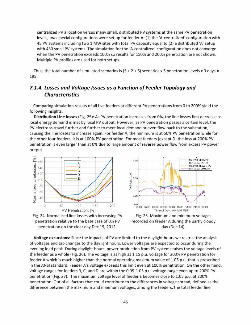
45

centralized PV allocation versus many small, distributed PV systems at the same PV penetration levels, two special configurations were set up for feeder A: (1) the ‘A-centralized’ configuration with 45 PV systems including two 1 MW sites with total PV capacity equal to (2) a distributed ‘A’ setup with 430 small PV systems. The simulation for the ‘A-centralized’ configuration does not converge when the PV penetration exceeds 100% so results for 150% and 200% penetration are not shown. Multiple PV profiles are used for both setups.

Thus, the total number of simulated scenarios is (5 + 2 + 6) scenarios x 5 penetration levels x 3 days =

195.

7.1.4. Losses and Voltage Issues as a Function of Feeder Topology and Characteristics

Comparing simulation results of all five feeders at different PV penetrations from 0 to 200% yield the following insights:

Distribution Line losses (Fig. 25): As PV penetration increases from 0%, the line losses first decrease as local energy demand is met by local PV output. However, as PV penetration passes a certain level, the PV electrons travel further and further to meet local demand or even flow back to the substation, causing the line losses to increase again. For feeder A, the minimum is at 50% PV penetration while for the other four feeders, it is at 100% PV penetration. For most feeders (except D) the loss at 200% PV penetration is even larger than at 0% due to large amount of reverse power flow from excess PV power output.

Fig. 24. Normalized line losses with increasing PV

penetration relative to the base case of 0% PV penetration on the clear day Dec 19, 2012.

Fig. 25. Maximum and minimum voltages recorded on feeder A during the partly cloudy

day (Dec 14). Voltage excursions: Since the impacts of PV are limited to the daylight hours we restrict the analysis

of voltages and tap changes to the daylight hours. Lower voltages are expected to occur during the evening load peak. During daylight hours, power production from PV systems raises the voltage levels of the feeder as a whole (Fig. 26). The voltage is as high as 1.15 p.u. voltage for 200% PV penetration for feeder A which is much higher than the normal operating maximum value of 1.05 p.u. that is prescribed in the ANSI standard. Feeder A’s voltage exceeds this limit even at 100% penetration. On the other hand, voltage ranges for feeders B, C, and D are within the 0.95-1.05 p.u. voltage range even up to 200% PV penetration (Fig. 27). The maximum voltage level of feeder E becomes close to 1.05 p.u. at 200% penetration. Out of all factors that could contribute to the differences in voltage spread, defined as the difference between the maximum and minimum voltages, among the feeders, the total feeder line

46

length has the strongest correlation with the voltage spread. The strong correlation is a result of the fact that a larger voltage drop occurs over a longer feeder line with the same amount of power flow and impedance, thus increasing the voltage spread. Therefore, the feeder hosting capacity (defined as the maximum level of PV penetration at which the voltage spread is in a permissible range) is expected to be a strong function of the feeder length.

Tap operations: Transformers and voltage regulators are programmed to change their tap position to keep voltage levels along the feeder within permissible limits. Fig. 28 shows the change in the number of tap operations for each feeder on the partly cloudy day. Feeder A experienced a very high increase in the number of tap operations in comparison to the other four due to a combination of its larger number of transformers and voltage regulators (Table 10) and large range of voltages (Fig. 27). There is no change in tap operations on feeder B even at 200% PV penetration due to its small voltage range. For feeder D, the only change is from 50% to 100% PV penetration and two tap operations are sufficient to manage 200% penetration.

Fig. 26. Voltage ranges on the partly cloudy day Dec 14 between 0700 to 1600 PT for all feeders. The timestamps above and below the bars show

when the extremes occur.

Fig. 27. The normalized total number of tap operations on the partly cloudy day relative to

the tap operations at 0% penetration level. At 0% penetration feeders A, B, C, D, and E have 219, 0, 7, 0, 15 tap operations, respectively. Feeder B has

zero tap operations at all PV penetration levels. Feeder D shows 2 tap operations for penetration

levels > 50%.

7.1.5. Single vs. Multiple PV Irradiance Profiles

The use of the single profile causes PV systems over the entire feeder to ramp synchronously, leading to more severe power fluctuations. This is unrealistic, especially for feeders with large footprints as the correlation between GHI between sites decreases exponentially with distance. To quantify and compare the fluctuation in voltages between the two configurations, we calculate the voltage volatility as standard deviation. Except for feeder A, the voltage is consistently more volatile when using a single PV profile at all PV penetration levels. The abnormality of feeder A’s volatility is due to the large number of voltage regulators which operate differently in response to various voltage fluctuating scenarios. Similarly, the single PV profile configuration overestimates the line losses (normalized using the 0% PV case in Fig. 29) in the feeder except for feeder A at 50 and 100%, and feeder D at 50% PV penetration cases. The overestimation amount is significant especially at very high PV penetration levels with 3% overestimation at 200% penetration, on average.

47

Fig. 28 Normalized line losses relative to the 0% penetration case for all five feeders with single and multiple PV profiles configurations on the

partly cloudy day.

Fig. 29. Max voltage recorded from five feeders with single and multiple PV profiles

configurations on the partly cloudy day.

Peak voltages generally occur at minimum net load which occurs during midday at high PV penetration.

Since the partly cloudy day does not contain a long clear period near the maximum daily generation, one would expect that the peak PV generation and therefore the maximum feeder voltage are also artificially enhanced if a single PV profile is considered. Indeed, the use of single PV profiles overestimates the maximum voltages for all five feeders by an increasing amount with increasing PV penetration (Fig. 30). The overestimations for maximum voltages at 200% PV for the five feeders are 0.0151, 0.0009, 0.0017, 0.0005, and 0.0064 p.u. voltage respectively.

However, the primary effect of distributed PV profiles is the reduction of PV power ramp rates and ramp

magnitudes that is expected to lead to a reduction in voltage regulator actions which directly affects the lifetime of voltage regulators and transformers. Indeed the number of tap operations on feeders A, C, and E (Fig. 31) decreases substantially. Feeders B and D require very few tap operations (0 and 2 respectively) even at 200% PV penetration so the different PV profiles do not make any difference. The use of a single profile overestimates significantly the number of tap changes for days with clouds (i.e. partly cloudy and overcast conditions), but not on clear days, as expected (Fig. 32). Specifically, for feeder A the overestimation percentages for the partly cloudy and overcast days are 260% and 245% at 50% PV penetration, and 127% and 131% at 200% PV penetration respectively. This shows the unique feature of our approach in which we model the PV production output more realistically and estimate the actual tap changing operations more accurately, especially during cloudy condition.

48

Fig. 30. Normalized tap operations of five feeders with single and multiple PV profiles

configurations on the partly cloudy day.

7.1.6. Distributed versus Centralized PV

The use of distributed PV systems reduces the power ramps significantly further in both frequency and magnitude (Fig. 33). The cause and effect is similar as for disaggregation as the PV capacity of a large PV system where all panels essentially ramp synchronously is redistributed across the feeder. Therefore the distributed PV power output is smoothed out by summing the power of many small PV systems that do not fluctuate synchronously. Thus, centralized PV on the feeder is much more prone to cause over-voltages due to large power generation, in particular if voltage regulators are not strategically placed to accommodate the heterogeneous concentration of PV on the feeder.

Fig. 31. Normalized tap operations of feeder A with single and multiple PV profiles

configurations on three days with different cloud conditions.

Fig. 32. Net power consumption recorded at the substation at 100% PV penetration for ‘A-

centralized’ and ‘A’ (distributed) configurations.

Furthermore, a centralized setup at high PV penetration level will suffer significantly more severe

voltage fluctuations than a distributed setup (Fig. 34). The upper voltage limit of 1.05 p.u. is violated by the A-centralized configuration even at 100% PV penetration while the A-distributed configuration does not violate this limit even at 200% PV penetration.

Fig. 33. Voltage range at different PV penetration

levels of the centralized and distributed configurations of feeder A.

Fig. 34. Comparison in number of tap operations between A-centralized and A-distributed

49

configurations at different PV penetration during daylight hours on Dec 14.

The A-centralized configuration also significantly increases the number of tap operations in

comparison to A-distributed (Fig. 35). Specifically, the A-centralized case has 295% and 192% more tap operations at 25% and 100% PV penetration respectively. Lastly, while line losses in the A-distributed configuration decrease with increasing PV penetration up to 100%, they increase again after PV penetration reaches 50% in the A-centralized setup (Fig. 36). Thus, the A-distributed setup would be a preferred choice if minimizing line losses is the objective.

Fig. 35. Total line loss during daylight hours of the centralized and distributed PV configurations at

different PV penetration on Dec 14th.

7.1.7. Conclusions

The project team proposed a new approach to study the impact of high PV penetration on a distribution network and its hosting capacity. The proposed method combines high resolution resource assessment using sky imagery with power system simulation on real distribution models to study the impacts of up to 200% PV penetration level on voltage excursions, line losses, and tap changing operations. We capture the unique temporal variation in power generated by each PV system in a highly realistic fashion. We conclude the following: A-Distributed vs. A-centralized PV: Scenario A-centralized has two large 1 MW PV system located close together which constitutes nearly 90% of the total PV capacity in the system. On the other hand, Scenario A-distributed does not contain large PV installations and the numerous smaller PV installations were more-or-less evenly distributed along the feeder. For the centralized PV Scenario, the tab changing operations were more frequent and the line losses were larger compared to the distributed PV Scenario. It is important to note that this tendency is not necessarily a general conclusion that applies to all feeders, but it shows that the distribution of the PV on the feeder has a significant impact on both the tap changing operations and the losses. Centralized PV on the feeder is also much more prone to cause overvoltages – in particular if voltage regulators are not strategically placed to accommodate the PV concentration on the feeder. PV increases operation of tap changers on partly cloudy days for some feeders: While two feeders can be managed with two or less tap changes even at 200% penetration, for the other feeders tap changes significantly increase especially for penetrations greater than 50%. Tap changers during cloudy days in the 100% PV penetration are operating 20 to 1,300 times each day (depending on the feeder) which is significantly higher than the number of tap changer operations for the no PV and low PV penetration Scenario (7 to 200 operations) and the clear-day simulation. This indicates that tap changing operations

50

during cloudy days will significantly increase if PV penetration levels are high, which can substantially increase maintenance costs and lifecycle costs of voltage regulators. On the other hand, for low PV penetration levels and during clear days, the tap changing operations is not impacted much. 4. Effect of disaggregating PV irradiances: For the high PV penetration Scenarios, disaggregation of the PV generation does reduce the number of tab changing operations significantly (to about half, on average). This indicates that aggregating the PV in simulations may exaggerate the actual tap changing operations that would occur on a real life system substantially. 5. PV reduces line losses: The presence of PVs significantly reduces line losses on the feeder. For 100% PV penetration Scenario 1, line losses are reduced by about 50 to 70% during daytime on partly cloudy days. We attribute the reduction of line losses to the fact the PV generation is much closer to the load compared to the no PV scenarios in which the power is supplied from the substation. Disaggregating PV power profiles further reduces the line losses. Note that our simulations do not account for transmissions losses that occur during the transfer of power from the plant to the substation. Accounting for these losses would increase the difference between losses without PV on the system and losses with PV on the system even more. 7.2. Solar Forecasting for Mitigating Distribution Feeder Impacts

7.2.1. Cause and effects of large amounts of tap operations

As shown in Chapter 7.1., the variation of the power output from PV arrays, particularly at high penetration levels, may cause serious voltage fluctuations on the feeder. To compensate such voltage variations and prevent them from exceeding the ANSI voltage limits, OLTCs are required to be operated. High PV penetration on a feeder may impose a high volume of switching operation on the voltage regulation devices, especially transformer OLTCs.

Typical number of TO of diverter switches for power transformers is approximately 20 per day, which makes the replacement of the contacts unnecessary during the life of transformers. The high number of TO for feeder A, which exceeds 250 TO/day for one of OLTCs, makes this feeder an interesting case to study the performance of the model predictive algorithm on both number/depth of TO and voltage quality. Feeder A has 7 transformers equipped with 32-step OLTCs with minimum and maximum ratios of 0.9 and 1.1. The voltage excursion due to such PV variability in the morning causes the OLTC of the closest transformer to the end of the feeder, i.e. Transformer 3, to perform a high volume of TO as shown in Fig. 37. A comparison between the curves shown in Fig. 37 explicitly shows the direct relation between PV variability and TO number/depth. Due to the partly cloudy weather on this day, the OLTC on transformer 3 is required to perform 177 TO with a total depth of 500 from 0800 to 1600 PST, which is equivalent to 50 TO depth per hour. At the time period from 1000 to 1100 PST, which is focused in Fig. 37b, the high variability of PV imposes 38 TO with a total depth of 135 on transformer 3 in just one hour. Such high-frequency TO put extra pressure on the moving parts of the tap changer and introduce remarkable wear and tear costs into operation cost of the entire system. However, in partly cloudy weather, such TO may be unnecessary and could be eliminated.

51

(a)

(b)

Fig. 36 Simulation results for feeder A at 100% penetration level on Jan 19, 2015 with 30-second resolution, along with a zoom into an especially variable period from 1000 to 1100 PST. (a) Total power output of 39 PV systems

installed downstream of transformer 3 (b) Tap position sequence of transformer 3. These 39 PV systems form 27% of total PV capacity on the feeder since both large PV systems are downstream of transformer 3.

7.2.2. Simulation setup and tap control algorithm

The study is carried out on the feeder A and the distribution system simulation results for feeder A described in Section 7.1. Here the same sky images are used to generate PV forecast data as described in Section 6.2. Applying forecasted solar generation and load of the feeder at each time step Ts, the operator is able to simulate the next 5 minutes of the power system to identify the optimal tap positions for each all transformer at every 30-second time step in [𝑇𝑇𝑓𝑓,𝑇𝑇𝑓𝑓 + 5 min]. The main objective is to perform the minimum possible number of TO. There are two scenarios where reducing the number and/or the depth of TO could be beneficial.

If the predicted sequence of tap position at [Ts, Ts + 5] shows that the tap would go back or cross over the same tap position applied at t = Ts-0.5, no TO is suggested. Therefore, the same tap position is maintained and both number and depth of TO is reduced.

If the predicted tap sequence in the entire period [Ts, Ts + 5] is expected to be higher than the actual tap position at t = Ts-0.5, the new tap position is selected equal to the minimum expected tap position . Mathematically,

OLTC[Ts, Ts + 0.5] = min�OLTCsim[Ts, Ts + 5]�

The reverse applies if the tap position is predicted to be always less than the current tap position. This action reduces the depth of TO, while it does not affect the number of TO.

To demonstrate the efficiency of the TO reduction method, it is tested on feeder A for 95 days between December 6, 2014 through March 15, 2015 for 100% PV penetration level. First, the base case simulations are carried out without applying the predictive tap changer control. This scenario is noted as ‘No Control’ scenario. Then, a 5-minute predictive tap changer control using the available forecast data at each time step is applied to observe its impact on both TO reduction and voltage quality. This

52

scenario is noted as ‘Actual Forecast’. To evaluate the robustness of the actual forecast scenario against sky imager PV forecast error, the simulations are repeated by employing the actually recorded PV outputs and this scenario is denoted as ‘Perfect Forecast’.

7.2.3. Simulated reduction in tap operations

Before examining the statistics of the simulation results, it is helpful to consider an example to show how different TO control scenarios reduce TO activities on OLTCs. Fig. 38 illustrates the one-hour window from 1000 through 1100 PST on January 19, 2015 with the tap position sequences of transformer 3 for different scenarios. In the “no control” scenario (base case), high variability of PV imposes 38 TO with a total depth of 135. Applying the perfect forecast scenario significantly reduces the number of TO to only one TO with depth of 2 taps, while the actual forecast scenario decreases the number and depth of TO to 9 and 17 respectively.

Fig. 37. Tap position sequences of transformer 3 at 10am-1pm on Jan 19, 2015 for three different scenarios.

According to the 95-day simulation results, the maximum daily TO reduction and TO depth reduction are equal to 71.11% and 80.36% respectively. On average, employing the tap reduction method decreases the daily number of TO from 461 to 247 TO per day, i.e., 46.5% reduction, while perfect forecasts reduce the number further to 251 TO/day resulting 45.5% reduction. The simulation results also show that the TO depth can be reduced from an average of 761 taps per day to 334 taps per day (54.12% reduction) by actual forecast scenario while it could be decreased to 344 taps per day if the forecast is perfect.

Fig. 39 illustrates the depth of TO by transformer in different control scenarios. Among the transformers connected to feeder A, the 3rd and 7th transformers show the highest and lowest share of TO depth, respectively. These results are consistent with the fact that transformer 7 is the closest to the substation where the voltage is almost constant, while transformer 3 is the closest one to the end of the feeder and more prone to voltage excursions due to the large adjacent PV system. The simulation results show that both tap reduction scenarios with actual and perfect forecasts offer significant advantages and similar performance. The depth of TO of transformers 2 and 3 is reduced by 66% to about 50 and 60 TO/day which is much closer to the typical value for normal power transformers of 20 TO/day.

Fig. 40 shows the relationship between the depth of tap reductions and the possibility for the control algorithms with actual forecast scenario to reduce unnecessary TO for each transformer. The higher the depth of TO, the higher is the percentage of TO reduction, but some transformers offer less potential for TO reductions than others. For example, the 95 values for daily TO depth of transformer 7 lying in [0, 50] taps per day lead to only 1.6% TO depth reduction for this transformer. On the other hand, transformers 1, 2, and 3 show the largest TO depth reduction for a given initial depth of taps per day. This is likely

53

because transformers 1, 2, and 3 are upstream of the large PV systems at the end of the feeder and therefore most exposed to high frequency variability.

Fig. 38. Impact of different control algorithms (no control, actual forecast, perfect forecast) on TO depth of transformers.

Fig. 39. Reduction in depth of TO using actual forecast scenario versus the initial depth of TO

per day for individual transformers.

7.2.4. Adverse impacts on voltage violations

Although the tap reduction control algorithms reduce the number/depth of TO, they may affect the voltage quality adversely. Therefore, it is crucial to investigate the voltage profile over the feeder in response to applying the proposed TO schedules. Fig. 41 illustrates the maximum and minimum voltages that occurred on feeder A on 95 days of simulations for different control scenarios. These results show that while such voltage excursions are rare, the occasional forecast error can result in temporary large voltage deviations. On some days, even the perfect forecast does not avoid voltage deviations.

However, according to the simulation results shown in Fig. 42a, the maximum voltage values in the TO reduction scenarios exceed 1.1 p.u. only about 0.2% of the simulation time, which is equal to 3 minutes per day. The results presented in Fig. 42b also demonstrate that the minimum voltages caused by actual and perfect forecast scenarios exceed the minimum threshold (0.95 p.u.) in just 5 and 8 time steps during the 95 days of simulations, i.e. 0.01% of the time.

Fig. 40. a, left) Daily maximum voltages on 95 days for different control methods, b, right) Daily minimum voltages on 95 days for different control methods

54

(a)

(b)

Fig. 41. a) Histogram of maximum voltage values on 95 days for different control methods, b) Histogram of

minimum voltages on 95 days for different control methods

7.2.5. Conclusions

A control strategy to reduce OLTC operations resulting from high PV penetration on distribution feeders was developed and applied. The strategy uses 5 minutes ahead solar forecast to derive future voltages states on the distribution feeder. Unnecessary TO are identified as those that are reversed within 5 minutes, likely because of temporary cloudy or clear conditions over adjacent PV systems.

On a feeder where TO were abundant at over 750 per day on average, the strategy resulted in the avoidance of 56% of the TO, which results in a significant savings in OLTC maintenance costs. Average extreme voltages were not affected by applying the TO reduction techniques. While the deviation of daily maximum and minimum voltage slightly increased on several days, a statistical analysis demonstrated that these deviations happened very rarely.

The strategy is most effective on partly cloudy days and on voltage regulators with a large number/depth of TO, but the voltage quality might be adversely affected on these days. The fraction of avoided TO decreased substantially for less than 10 to 40 original TO per day, depending on the voltage regulator.

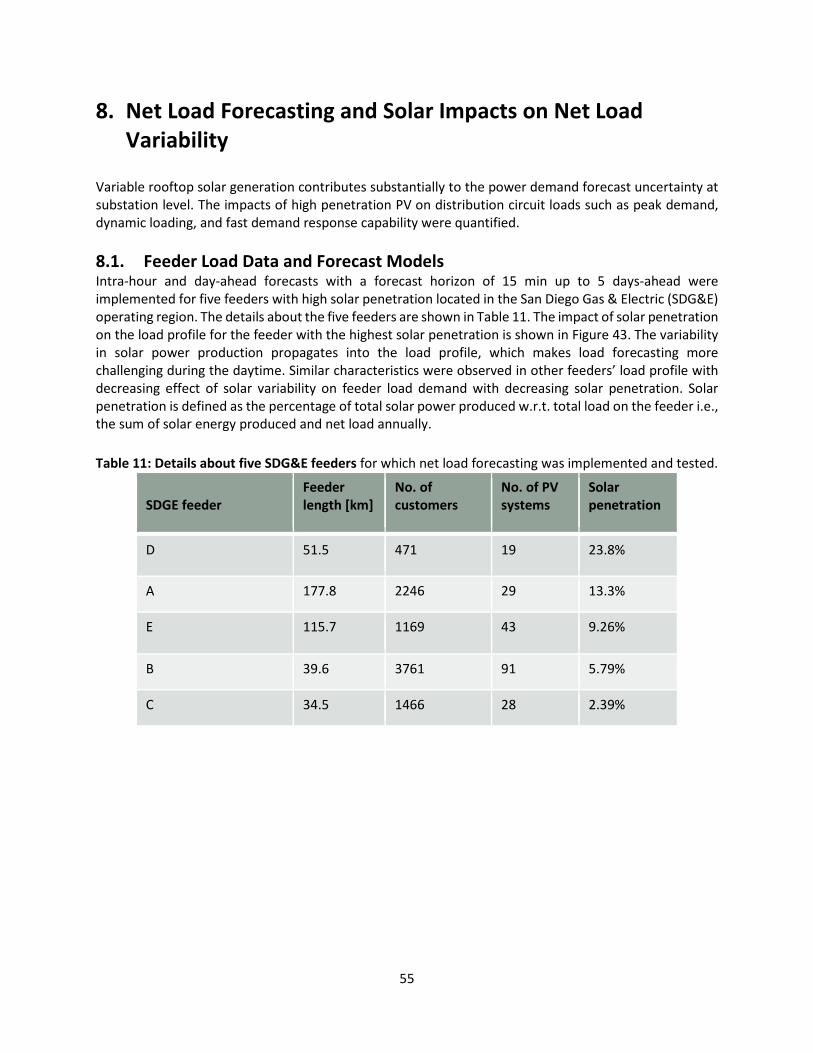
55

8. Net Load Forecasting and Solar Impacts on Net Load Variability

Variable rooftop solar generation contributes substantially to the power demand forecast uncertainty at substation level. The impacts of high penetration PV on distribution circuit loads such as peak demand, dynamic loading, and fast demand response capability were quantified. 8.1. Feeder Load Data and Forecast Models Intra-hour and day-ahead forecasts with a forecast horizon of 15 min up to 5 days-ahead were implemented for five feeders with high solar penetration located in the San Diego Gas & Electric (SDG&E) operating region. The details about the five feeders are shown in Table 11. The impact of solar penetration on the load profile for the feeder with the highest solar penetration is shown in Figure 43. The variability in solar power production propagates into the load profile, which makes load forecasting more challenging during the daytime. Similar characteristics were observed in other feeders’ load profile with decreasing effect of solar variability on feeder load demand with decreasing solar penetration. Solar penetration is defined as the percentage of total solar power produced w.r.t. total load on the feeder i.e., the sum of solar energy produced and net load annually. Table 11: Details about five SDG&E feeders for which net load forecasting was implemented and tested.

SDGE feeder

Feeder length [km]

No. of customers

No. of PV systems

Solar penetration

D 51.5 471 19 23.8%

A 177.8 2246 29 13.3%

E 115.7 1169 43 9.26%

B 39.6 3761 91 5.79%

C 34.5 1466 28 2.39%

56

Figure 42 Sample satellite image and load profile for 21 March 2013 for a highly cloudy day. The red circle in the satellite image shows the feeder location. The effect of solar penetration on the load profile manifests in the load fluctuations during daytime [7:00 – 18:00 PDT].

For developing and testing the models, the dataset was divided into two disjoint datasets: the training set consists of data between January 2011 to June 2012 and the validation/testing set ranges from July 2012 to June 2013. For intra-hour forecasts, methods with non-exogenous inputs were implemented, whereas for multiple day ahead forecast, day- ahead solar irradiance forecasts provided by the NOAA North American Model (NAM) were also used as inputs. The forecast models with non-exogenous input were developed as �̀�𝑦(𝑡𝑡 + 𝑘𝑘|𝑡𝑡) = 𝑓𝑓 (𝑦𝑦(𝑡𝑡),𝑦𝑦(𝑡𝑡 − 1),𝑦𝑦(𝑡𝑡 −2) …𝑦𝑦 (𝑡𝑡 − 𝑛𝑛𝑘𝑘)), where ‘𝑦𝑦’ is the net load, ‘�́�𝑦’ is the net load forecast issued at time ‘𝑡𝑡’ for ‘𝑘𝑘’ steps ahead (forecast horizon) using a non-linear/linear function, ‘ 𝑓𝑓 ‘ with ‘𝑛𝑛𝑘𝑘’ as the number of time-lagged inputs. If no information about the underlying processes affecting the system is available, machine-learning tools like Artificial Neural Networks (ANN) and Support Vector Regression (SVR) have proven to be useful for input/output mapping. ANNs consist of multiple layers with processing units called neurons. Neurons take in weighted sum of inputs through various layers and produce an output using an activation function. For this study, the optimal structure of the ANN was obtained by using a Genetic Algorithm (GA). GA is an optimization algorithm based on survival of the fittest individuals (Pedro and Coimbra, 2012). Secondly, a non-linear regression technique known as Support Vector Regression (SVR) was applied (Vatnik et al. 1997). Moreover, pattern recognition-based machine learning techniques i.e., k-Nearest Neighbors (kNN) were also implemented for day ahead load forecasting. This technique identifies similar patterns in the historical dataset w.r.t. the present conditions and chooses the closest neighbors. For this study 15 best neighbors were chosen. The corresponding outputs of the best neighbors are combined to issue a forecast (Kaur et al. 2013). Finally, NAM weather forecasts are used as an input to day-ahead forecasts by utilizing an ensemble re-forecast method (Kaur et al. 2014). The ensemble re-forecast method is a combination of various linear and non-linear time-series regression techniques like autoregressive model with exogenous input (ARX), non-linear autoregressive model with exogenous input (NARX), Box-Jenkins model (BJ), etc. Validation was conducted with error metrics described in Section 2. 8.2. Intra-hour Forecast Results Machine learning based forecasting models were developed for intra-hour forecasting for 15 min, and 30 min forecast horizon with 15 min averaged time-series as provided by SDG&E. Since the load profile is

57

inherently different during daytime compared to night time due to variability introduced by solar energy, two local SVR models for each feeder were developed: one for day time and another one for night time. Comparing the results using SVR and ANN from Table 12, it can be observed that the performance of both methods is similar for the 15 min forecast horizon. ANN-GA outperforms SVR for 30 min forecast horizon in terms of MAPE. The sample results using local SVR are shown in Figure 44 for feeder D to compare the accuracy of the forecasting model for clear and cloudy conditions. Most of the error occurs during the daytime especially during cloudy days. The impact of intermittency in solar power can be observed in net load, which are challenging to forecast resulting in high magnitude forecast errors. Also, despite the fact that feeders E and C have lower solar penetration as compared to feeder D and A, they still have high forecasting error. These high magnitude errors for feeders E and C can be attributed to the high variability in load from these feeders independent of solar generation (see Figure 45). Next, the intra-hour SVR forecast models were extended for multiple day(s) ahead forecasting. Table 12 Net load forecast results for 15 min forecast horizon for the five feeders.

Models SVR GA/ANN

Feeder- Solar Penetration

MAPE [%], RMSE [MW], R2 MAPE [%], RMSE [MW], R2

D – 23.8% 5.06 0.10 0.96 5.24 0.10 0.96

A – 13.3% 2.54 0.19 0.97 2.83 0.17 0.97

E – 9.2% 2.39 0.05 0.95 3.34 0.05 0.95

B – 5.8% 2.24 0.11 0.98 1.92 0.09 0.99

C – 2.4% 2.40 0.07 0.98 2.76 0.06 0.99

58

Figure 43: Load forecast results for feeder D for 15 min forecast horizon using SVR. The first two days are clear days whereas the next two days depict cloudy days. The absolute error increases for cloudy days especially during solar production time. The vertical dashed lines indicate midnight PDT time.

Figure 44 Load profile for feeder E for 04-14-2013 to 04-28-2013. It can be seen that the load profile for this feeder has high variability with sudden increase in load demand with no correlation to the past values. These spikes in load demand makes load forecasting very challenging with no information available about the sudden increase. 8.3. Solar variability and solar penetration effects on intra-hour load forecasts Next, the impact of solar variability and the level of solar penetration on intra-hour load forecast capabilities was studied using the synthetic high-resolution satellite-derived 𝐺𝐺𝐺𝐺𝐺𝐺 utilized in Chapter 3. Ramps, 𝑅𝑅(𝑡𝑡) at time (𝑡𝑡) for 30 min time-scale were defined as 𝑅𝑅(𝑡𝑡) = 𝐺𝐺𝐺𝐺𝐺𝐺(𝑡𝑡) − 𝐺𝐺𝐺𝐺𝐺𝐺 (𝑡𝑡 − 1). Since the resolution for satellite-derived data was 30 min, separate forecasts were produced for the 30 min forecast horizon for 30 min averaged load time-series. Hence, the MAPE for these forecasts is lower than the

59

forecast issued at 30 min forecast horizon for 15 min time-averaged values as many ramps at 15 min timescale average out at 30 min time-scale. It was observed that the load forecast error is independent of solar variability for feeders with low solar penetration. As solar penetration increases, the load forecast error increases and is a linear function of solar variability. As shown in Figure 46, the error increases linearly with increasing solar variability for the feeder D load which has highest solar penetration. In contrast to that, the error for feeder C (the feeder with lowest solar penetration) is uniform and stays the same irrespective of the solar variability.

Figure 45 Net load forecast error versus irradiance variability. Normalized absolute forecast error for the 30 min forecast horizon using SVR versus solar variability for the five feeders. 𝑨𝑨𝒕𝒕 is the actual value of the load, 𝑭𝑭𝒕𝒕 is the forecast value for time 𝒕𝒕 and ∆ represents the change in Global Horizontal Irradiance at every 30 min time step. The error is independent of the solar variability for feeders with lowest penetration (e.g. feeder C). With increasing solar penetration, the load forecast error increases and appears to be a linear function of solar variability. 8.4. Days-ahead forecast results Forecasts were implemented for 1 – 5 days ahead with hourly resolution. The MAPE for each feeder for all the forecast horizons is shown in Figure 47. These forecasts are based on SVR and kNN model. The input vectors are the lagged values for the same hour from the past seven days. The MAPE for all feeders increases with increasing forecast horizon, eventually approaching a constant value. Since the forecast for more than four days-ahead is giving information just about the shape of load profile like a polynomial fit, the error remains constant. Contrary to the expected result that the feeder with the highest penetration

60

would contain the highest MAPE, feeder E has the highest MAPE irrespective of the forecast horizon. This can be again attributed to its load profile as discussed in Figure 45.

Figure 46 Day ahead net load forecast error. Mean Absolute Percentage Error for all the feeders using SVR.

Figure 47 Load forecast results for feeder D for the 24h forecast horizon (top) and Absolute Error (AE) at the same times (bottom) for the year 2013 using SVR. The AE increases during daytime due to varying solar generation. The timestamps are in PDT. The above results were obtained without exogenous inputs. This demonstrates the challenging time-series characteristics for the day-ahead forecast horizon, in part due to ramps introduced by varying solar power generation. Sample intra-day forecasts are shown in Figure 48. To correct for these errors, an

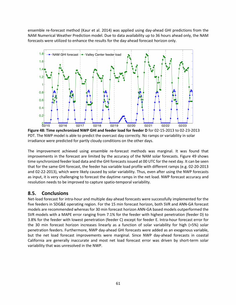
61

ensemble re-forecast method (Kaur et al. 2014) was applied using day-ahead GHI predictions from the NAM Numerical Weather Prediction model. Due to data availability up to 36 hours ahead only, the NAM forecasts were utilized to enhance the results for the day-ahead forecast horizon only.

Figure 48: Time synchronized NWP GHI and feeder load for feeder D for 02-15-2013 to 02-23-2013 PDT. The NWP model is able to predict the overcast day correctly. No ramps or variability in solar irradiance were predicted for partly cloudy conditions on the other days. The improvement achieved using ensemble re-forecast methods was marginal. It was found that improvements in the forecast are limited by the accuracy of the NAM solar forecasts. Figure 49 shows time synchronized feeder load data and the GHI forecasts issued at 00 UTC for the next day. It can be seen that for the same GHI forecast, the feeder has variable load profile with different ramps (e.g. 02-20-2013 and 02-22-2013), which were likely caused by solar variability. Thus, even after using the NWP forecasts as input, it is very challenging to forecast the daytime ramps in the net load. NWP forecast accuracy and resolution needs to be improved to capture spatio-temporal variability. 8.5. Conclusions Net-load forecast for intra-hour and multiple day-ahead forecasts were successfully implemented for the five feeders in SDG&E operating region. For the 15 min forecast horizon, both SVR and ANN-GA forecast models are recommended whereas for 30 min forecast horizon ANN-GA based models outperformed the SVR models with a MAPE error ranging from 7.1% for the feeder with highest penetration (feeder D) to 3.8% for the feeder with lowest penetration (feeder C) except for feeder E. Intra-hour forecast error for the 30 min forecast horizon increases linearly as a function of solar variability for high (>5%) solar penetration feeders. Furthermore, NWP day-ahead GHI forecasts were added as an exogenous variable, but the net load forecast improvements were marginal. Since NWP day-ahead forecasts in coastal California are generally inaccurate and most net load forecast error was driven by short-term solar variability that was unresolved in the NWP.

62

References Reports Completed under this Agreement Reports are available at http://www.calsolarresearch.org/funded-projects/87-high-fidelity-solar-forecasting-demonstration-for-grid-integration.

• Task 5 Final Report: Substation Net Load Operational Forecasts for Fast Demand Response Implementation. Kaur, A., Nonnenmacher, L., and Coimbra, C. Center for Renewable Resources and Integration, UCSD. Jan 27, 2015. PDF (741 KB)

• Net Load Forecasting with Distributed Generation. Green Power Labs. Dec 16, 2014.PDF (3 MB)

• Recommend placement and operation of SDG&E weather stations to maximize forecast effectiveness. Coimbra Energy Group, UCSD. Mar 2014.PDF (1.5 MB)

• Ensemble Forecasting of Solar Irradiance in Coastal Southern California. Ozge Akyurek, B., Zhong, X., and Kleissl, J. UCSD. Jan 24, 2015. PDF (2 MB)

• Aggregate Ramp Rates Analysis of Distributed PV Systems in 5 Locations at San Diego County. Bosch, Juan L., Jamaly, M., and Kleissl, J. Dept. of Mech & Aerospace Eng., University of California, San Diego. February 6, 2013. PDF (8 KB)

• Marine Layer Forecasting Report. Green Power Labs. May 30, 2014. PDF (5 MB)

• <ADD Task 4.2, 4.3, 4.4 reports>

The following three reports were developed as part of California Energy Commission and Department of Energy funded work as cost-share:

• Observability of Microgrid Operations by the California Independent System Operator. Final Project Report. Torre, William V. Center for Energy Research Department of Electrical and Computer Engineering University of California, San Diego. April 2014.PDF (1.7 MB)

• Improved Modeling Tools Development for High Penetration Solar. UCSD: Byron Washom, Byron, Kleissl, J., Nottrott, A., Hanna, R., and Yang, H. Power Analytics Corp: Meagher, Kevin, Zhang, Y, and Koopman, R. Prepared for the U.S. Dept. of Energy. March 2014. PDF (6 MB)

• Intra-hour Solar Power Forecasting at Utility-scale Power Plants in the Los Angeles Basin. Final Project Review Draft. Babacan, Oytun, Wang, G., Yang, H., and Kleissl, J. Prepared for the California Energy Commission Public Interest Energy Research PIER Program. 2012. PDF (2 MB)

General References California Solar Initiative, "California Public Utilities Commission California Solar Initiative Program Handbook"," [Online]. Available: http://www.gosolarcalifornia.org/documents/CSI_HANDBOOK.PDF. [Accessed 15 Sep. 2011] Chow, C., Urquhart, B., Dominguez, A., Kleissl, J., Shields, J., & Washom, B. (2011). Intra-Hour Forecasting with a Total Sky Imager at the UC San Diego Solar Energy Testbed. Solar Energy, 85, 2881--2893.

63

Clean Power Research (2014), SolarAnywhere Irradiance Data, www.solaranywhere.com. Ghonima M, Urquhart B, Chow CW, Shields JE, Cazorla A, and Kleissl J (2012). A method for cloud detection and opacity classification based on ground based sky imagery. Atmospheric Measurement Techniques, Volume 5, pp. 4535-4569, doi:10.5194/amtd-5-4535-2012. Jamaly, M., J.L. Bosch, and J. Kleissl, Power Output Analysis of Distributed PV Systems in California Using SolarAnywhere Enhanced Resolution Irradiation, CSI Report, 2012. Jamaly, M., JL Bosch, J Kleissl, Aggregate Ramp Rates of Distributed Photovoltaic Systems in San Diego County, IEEE Transactions on Sustainable Energy, 99, 2012, 10.1109/TSTE.2012.2201966 Jamaly, M., J.L. Bosch, and J. Kleissl, Aggregate Ramp Rates Analysis of Distributed PV Systems in San Diego Gas & Electric Territory, 2013, California Solar Initiative RD&D Program website http://www.calsolarresearch.org/funded-projects/65-improving-economics-of-solar-power-through-resource-analysis-forecasting-and-dynamic-system-modeling. Kaur, A., H.T.C. Pedro, C.F.M. Coimbra, Impact of onsite solar generation on system load demand forecast, Energy Conversion and Management 75 (0) (2013) 701 – 709. Kaur, A., H.T.C Pedro, C.F.M. Coimbra, Ensemble re-forecasting methods for enhanced power load prediction, Energy Conversion and Management 80 (0) (2014) 582 – 590. Lopez-Coto, I., Patrick Mathiesen, Juan Luis Bosch, Brian D’Agostino, Brandt Maxwell, Robert Fovell and J Kleissl, A Comparison Between Several Parameterization Schemes in WRF for Solar Forecasting in Coastal Southern California, submitted to Monthly Weather Review. Mathiesen, P., C. Collier, and J. Kleissl, “A high-resolution, cloud-assimilating numerical weather prediction model for solar irradiance forecasting.“ Solar Energy, 2013.Pedro, H.T.C., C.F.M. Coimbra, Assessment of forecasting techniques for solar power production with no exogenous inputs, Solar Energy 86 (7) (2012) 2017 – 2028. Perez, R., P. Ineichen, K. Moore, M. Kmiecik, C. Chain, R. George, and F. Vignola, "A new operational model for satellite-derived irradiances: Description and validation," Solar Energy, 73(5):307-317, 2002. Skamarock, W., Klemp, J., Dudhia, J., Gill, D., Barker, D., Duda, M., Huang, X., Wang, W., Powers, J., 2008. A description of the advanced research WRF – version 3. NCAR Technical Note NCAR/TN 475+STR. Stein, J.S., C. W. Hansen and M. J. Reno, “The Variability Index: A new and novel metric for quantifying irradiance and PV output variability” ASES conference 2012. Urquhart, B., Mohamed Ghonima, Dung Nguyen, Ben Kurtz, Chi Wai Chow and Jan Kleissl, Sky Imaging Systems for Short-term Forecasting, in: Solar Resource Assessment and Forecasting (Editor Jan Kleissl), Elsevier, 2013 Vapnik, V., S. E. Golowich, A. Smola, Support vector method for function approximation, regression estimation, and signal processing, Advances in neural information processing systems (1997) 281–287.