draft 1 synthesis of reactive switching protocols from...

DRAFT 1

Synthesis of Reactive Switching Protocols

from Temporal Logic Specifications

Jun Liu, Necmiye Ozay, Ufuk Topcu, and Richard M. Murray

Abstract

We propose formal means for synthesizing switching protocols that determine the sequence in

which the modes of a switched system are activated to satisfy certain high-level specifications in

linear temporal logic (LTL). The synthesized protocols are robust against exogenous disturbances on the

continuous dynamics and can react to possibly adversarial events (both external and internal). Finite-

state approximations that abstract the behavior of the underlying continuous dynamics are defined using

finite transition systems. Such approximations allow us to transform the continuous switching synthesis

problem into a discrete synthesis problem in the form of a two-player game between the system and

the environment, where the winning conditions represent the high-level temporal logic specifications.

Restricting to an expressive subclass of LTL formulas, these temporal logic games are amenable to

solutions with polynomial-time complexity. By construction, existence of a discrete switching strategy for

the discrete synthesis problem guarantees the existence of a switching protocol that can be implemented

at the continuous level to ensure the correctness of the nonlinear switched system and to react to the

environment at run time.

Index Terms

Hybrid systems, switching protocols, formal synthesis, linear temporal logic, temporal logic games.

This work was supported in part by the NSERC of Canada, the FCRP consortium through the Multiscale Systems Center

(MuSyC), AFOSR award number FA9550-12-1-031, and the Boeing Corporation.

Jun Liu is with the Department of Automatic Control and Systems Engineering, University of Sheffield, Sheffield S1 3JD,

United Kingdom. Necmiye Ozay, Ufuk Topcu, and Richard M. Murray are with Control and Dynamical Systems, California

Institute of Technology, Pasadena, CA 91125, USA.

August 31, 2012 DRAFT

DRAFT 2

I. INTRODUCTION

The objective of this paper is to synthesize switching protocols that determine the sequence

in which the modes of a switched system are activated to satisfy certain high-level specifications

formally stated in linear temporal logic (LTL). Different modes may correspond to, for example,

the evolution of the system under different, pre-designed feedback controllers [24], so-called

motion primitives in robot motion planning [12], or different configurations of a system (e.g.,

different gears in a car or aerodynamically different phases of a flight). Each of these modes

may meet certain specifications but not necessarily the complete, mission-level specification the

system needs to satisfy. The purpose of the switching protocol is to identify a switching sequence

such that the resulting switched system satisfies the mission-level specification.

We are interested in designing open systems that can sense their environment and interact

with it by appropriately (as encoded by the specification) reacting to sensory inputs. Given a

family of system models, in the form of ordinary differential equations potentially with bounded

exogenous disturbances, a description of the sensed environment, and an LTL specification, our

approach builds on a hierarchical representation of the system in each mode and the environment.

In particular, we model environment as transition systems, which can be constructed through

observations of possibly continuous signals. While the continuous evolution of the system is

accounted for at the low level, the higher level is composed of a finite-state approximation of

the continuous evolution. The switching protocols are synthesized using the high-level, discrete

models. Simulation-type relations [1] between the continuous and discrete models guarantee that

the correctness of the synthesized switching protocols is preserved in the continuous implemen-

tation.

Our approach relies on a type of finite-state approximation for continuous nonlinear systems,

namely over-approximation. Roughly speaking, we call a finite transition system T an over-

approximation of the continuous system if for each transition in T , there is a possibility for

continuously implementing the strategy, in spite of either the exogenous disturbances or the

coarseness of the approximation. We account for the mismatch between the continuous model

and its over-approximation as nondeterminism and treat it as adversary. Consequently, the cor-

responding switching protocol synthesis problem is formulated as a two-player temporal logic

game (see [32] and references therein and the pioneering work in [9]). This game formulation


DRAFT 3

allows us to incorporate environment signals that do not affect the dynamics of the system but

constrain its behavior through the specification. Within the game, environment is also treated

as adversarial, that is, we aim to synthesize controllers that guarantee the satisfaction of the

specification even against the worst-case behavior of the environment.

The main contributions of the current paper are in (1) proposing a framework for switching

protocol synthesis for continuous-time nonlinear switched systems, potentially subject to exoge-

nous disturbances, from LTL specifications, and (2) synthesis of controllers that can continuously

sense their environment and react to the changes in the environment according to the specifi-

cation. In contrast to much of prior work (described in more detail below), we consider open

systems that can maintain ongoing interaction with some external environment and synthesize

controllers that are reactive to this environment. The use of LTL enables us to handle a wide

variety of specifications beyond mere safety and reachability. The game formulation allows us

to account for a potentially adversarial, a priori unknown environment in which the system

operates (and therefore its correctness needs to be interpreted with respect to the allowable

environment behaviors). While the general game structure considered in this paper can handle

full LTL specifications, such games with complete LTL specifications are known to have high

computational complexity [34]. Therefore, we focus on an expressive fragment of LTL, namely

Generalized Reactivity (1) (GR(1)) specifications, for which there exist synthesis algorithms with

favorable computational complexity [32].

Fragments of the switching protocol synthesis problem considered here have attracted consid-

erable attention. We now give a very brief overview of some of the existing work as it ties to the

proposed methodology (a thorough survey is beyond the scope of this paper). Stability problems

for switched systems arise naturally in the context of switching control and considerable work has

been focused on designing switching controllers for stability. Hespanha and Morse [16] propose

the notion of average dwell time, generalizing that of dwell time considered by Morse [29]. Both

dwell time and average dwell time are design parameters that can be chosen to achieve stability

when switching between stabilizing controllers. Jha et al. [18] focuses on switching logics that

guarantee the satisfaction of certain safety and dwell-time requirements. Taly and Tiwari [38],

Camara et al. [8], Asarin et al. [2], and Koo et al. [21] consider either switching controller

synthesis for safety [8], reachability [21], or a combination of safety and reachability properties

[2], [38]. Joint synthesis of switching logics and feedback controllers for stability are studied


DRAFT 4

by Lee and Dullerud [23]. The work by Frazzoli et al. [12] on the concatenation of a number

of motion primitives from a finite library to satisfy certain reachability properties constitutes an

instance of switching protocol synthesis problem. Our work also has strong connections with

the automata-based composition of the so-called interfaces that describe the functionality and

the constraints on the correct behavior of a system [41]. Also related is the work by Moor

and Davoren [28] who use modal logic to design switching control that is robust to uncertainty

in the differential equations. The objective there is to determine a control sequence to switch

among the family of differential equations to satisfy a specification that includes safety and event

sequencing. Our work extends these results both in terms of the family of models that can be

handled and the expressivity of the specification language used.

More broadly, this paper can be seen in the context of abstraction-based, hierarchical ap-

proaches to controller synthesis for continuous and hybrid systems from high-level specifications

given in terms of LTL [4], [11], [14], [19], [37]. Either by limiting the type of dynamical systems

considered [4], [14], [19] or by considering a rich (e.g., unconstrained) control input [11], [37],

which can arbitrarily steer the system, these papers obtain deterministic abstractions for the

underlying systems and use model-checking based methods for synthesis. The work by Tumova

et al. [40] extends this framework by allowing piecewise affine systems and nondeterministic

transitions in the abstraction. While allowing more flexibility in constructing the abstraction,

the presence of nondeterministic transitions render standard model checking tools no longer

applicable for finding a control strategy. Kloetzer and Belta [20] investigate this and propose a

solution inspired from (infinite) two-player LTL games. Compared to these results, the control

authority in our framework is fairly limited (i.e., only control input is the mode of the switched

system) which leads to a more challenging problem.

Beyond combining ideas from and extending results in switching protocol synthesis and

abstraction-based controller synthesis, the main difference between the aforementioned papers

[2], [4], [8], [11], [12], [14], [16], [18]–[21], [23], [28], [29], [37], [38], [40], [41] and the

work presented here is that, in those papers, the control strategy is non-reactive in the sense

that its behavior does not take into account external events from the environment at run time.

Such runtime reactiveness is crucial for satisfying safety properties. For instance, in cases of

emergency (e.g., in traffic when a pedestrian jumps on the street) the system might need to take

immediate action, or when a failure occurs, the system might need to deactivate the faulty parts


DRAFT 5

promptly for safe operation. Reactive controller synthesis, in particular by using GR(1) games,

has been considered before by Kress-Gazit et al. [22] and Wongpiromsarn et al. [44]. Kress-

Gazit et al. [22] consider systems with fully actuated dynamics (x = u), for which bisimilar

continuous implementations of discrete plans are guaranteed to exist. Although the environment

is continuously sensed in [22], one limitation of the method is that the controller is allowed

to take actions against the environment only when certain locative propositions are satisfied,

hence the system can not synchronously react to the environment at run time. Wongpiromsarn

et al. [44] focus on discrete-time linear time-invariant models with exogenous disturbances and

propose a receding horizon framework for alleviating the computational complexity. Reasoning

of continuous trajectories and environment behavior in continuous time is not a concern in

[44] either, as discrete-time models are considered. Abstractions considered in both papers are

deterministic in the sense that every transition between discrete states can be implemented,

whereas in the current paper we focus on over-approximations, which are potentially easier to

compute for switched nonlinear systems, where the controls are limited to the discrete modes.

Contrary to existing work, one of the major contributions of the paper is to achieve runtime

reactiveness of the continuous-time switching controller. To this end, we explicitly model the

environment and take into account possibly asynchronous interactions between the system dy-

namics and the environment. This is accomplished by defining product transition systems from

the abstractions and augmenting these transition systems with additional liveness conditions to

enforce progress in accordance with the underlying dynamics.

II. PRELIMINARIES

In this section, we introduce linear temporal logic (LTL) [27], [33] as the specification language

to formally specify system properties.

A. LTL syntax and semantics

Standard LTL is built upon a finite set of atomic propositions, logical operators ¬ (negation)

and ∨ (disjunction), and the temporal modal operators © (next) and U (until). LTL is a rich

specification language that can express many desired properties, including safety, reachability,

invariance, response, and/or a combination of these [27].


DRAFT 6

Syntax of LTL: Formally, the set of LTL formulas over a finite set of atomic propositions Π

can be defined inductively as follows:

(1) any atomic proposition π ∈ Π is an LTL formula;

(2) if ϕ and ψ are LTL formulas, so are ¬ϕ, ©ϕ, ϕ ∨ ψ, and ϕUψ.

Additional logical operators, such as ∧ (conjunction), → (material implication), and temporal

modal operators ♦ (eventually), and � (always), are defined by:

(a) ϕ ∧ ψ := ¬(¬ϕ ∨ ¬ψ);

(b) ϕ→ ψ := ¬ϕ ∧ ψ;

(c) True := p ∨ ¬p, where p ∈ Π;

(d) ♦ϕ := TrueUϕ;

(e) �ϕ := ¬♦¬ϕ.

A propositional formula is one that does not include any temporal operators.

Semantics of LTL: An LTL formula over Π is interpreted over ω-words, i.e. infinite sequences,

in 2Π. Let w = w0w1w2 · · · be such a word. The satisfaction of an LTL formula ϕ by w at

position i, written wi � ϕ, is defined recursively as follows:

(1) for any atomic proposition π ∈ Π, wi � π if and only if π ∈ wi;

(2) wi � ¬ϕ if and only if wi 2 ϕ;

(3) wi � ©ϕ if and only if wi � ϕ;

(4) wi � ϕ ∨ ψ if and only if wi � ϕ or wi � ψ;

(5) wi � ϕUψ if and only if there exists j ≥ i such that wj � ψ and wk � ϕ for all k ∈ [i, j).

The word w is said to satisfy ϕ, written w � ϕ, if w0 � ϕ.

LTL without next step: We denote the subset of the logic LTL without the next operator by

LTL\©.

B. Finite transition system

Definition 1. A finite transition system is a tuple T := (Q,Q0,→), where Q is a finite set of

states, Q0 ⊆ Q is a set of initial states, and →⊆ Q × Q is a transition relation. Given states

q, q′ ∈ S, we write q → q′ if the transition relation → contains the pair (q, q′).

We assume that for every state q ∈ Q, there exists a state q′ ∈ Q such that q → q′. Let

hQ : Q → 2Π be an observation map which maps the state space Q to a finite set of propositions.


DRAFT 7

Definition 2. An execution ρ : Z+ → Q of a finite transition system T = (Q,Q0,→) is an

infinite sequence ρ = q0q1q2 · · · , where ρ(0) = q0 ∈ Q0 and ρ(i) = qi ∈ Q and ρ(i)→ ρ(i+ 1)

(i ∈ Z+). The word produced by an execution ρ is wρ = wρ(0)wρ(1)wρ(2) · · · , where wρ(i) =

hQ(ρ(i)) for all i ≥ 0. An execution ρ is said to satisfy an LTL formula ϕ, written ρ � ϕ, if and

only if the word it produces satisfies ϕ. If all executions of T satisfy ϕ, we say that the finite

transition system T satisfies ϕ and write T � ϕ.

C. Continuous-time signals

Let X be a set (infinite or finite) and hX : X → 2Π be an observation map which maps X

to a finite set of propositions. A continuous-time signal s ∈ X is a function s : R+ → X .

Definition 3. We say that a signal s ∈ X is of finite variability (on bounded intervals of

R+) under observation hX if there exists an infinite number of non-overlapping intervals I =

I1, I2, · · · such that ∪∞i=1Ii = R+, hX(s(t)) = hX(s(t′)) for all t, t ∈ Ii, and l(Ij) → ∞ as

j →∞, where l(Ij) denotes the left end-point of Ij .

The above definition is similar to the notion of finite variability for continuous-time Boolean

signals [26]. Here the observation map is explicit and original signals need not to be of finite

variability. In the rest of the paper, unless otherwise stated, we restrict our attention to signals

that are of finite variability under some observation map.

Definition 4. Let s be continuous-time signal in X . The word produced by s is a sequence

ws = ws(0)ws(1)ws(2) · · · , defined recursively as follows:

• ws(0) = hX(s(0));

• ws(k) = hX(s(τ+k )) = limt→τ+k

hX(s(t)) for all k ≥ 1 such that τk < ∞, where τk is

defined by τ0 = 0 and τk = inf {t : t > τk−1, hX(s(t)) 6= ws(k − 1)} for all k ≥ 1; and

• ws(k) = ws(k − 1) for all k such that τk =∞.

The word ws is said to be well-defined if τk →∞ as k →∞. The signal s is said to satisfy an

LTL formula ϕ, written ρ � ϕ (s � ϕ), if and only if the word it produces is well-defined and

satisfies ϕ.

Intuitively, the word generated by a signal is exactly the sequence of sets of propositions

satisfied by the signal as time evolves. This definition is consistent with that of [19, Definition


DRAFT 8

4]. In the above definition, it is assumed that the limit hX(s(τ+)) = limt→τ+ hX(s(t)) for all

τ ≥ 0. This would exclude certain unrealistic signals such as those with observations 1 on

rationals and 0 on irrationals out of the scope. It is easy to check that the above definition is

well-posed and gives well-defined words for signals of finite variability.

III. PROBLEM FORMULATION

In this section, we introduce the system models and formulate the main problem studied in

this paper.

A. Continuous-time switched systems

Consider a family of nonlinear systems,

x(t) = fp(x(t), d(t)), p ∈ P , t ≥ 0, (1)

where x(t) ∈ X ⊆ Rn is the state at time t and d(t) ∈ D ⊆ Rd is an exogenous disturbance, P

is a finite index set, and {fp : p ∈ P} is a family of nonlinear vector fields satisfying the usual

conditions to guarantee the existence and uniqueness of solutions for each of the subsystems in

(1). A switched system generated by the family (1) can be written as

x(t) = fσ(t)(x(t), d(t)), t ≥ 0, (2)

where σ is a switching signal taking values in P . The value of σ at a given time t may depend

on t or x(t), or both, or may be generated by using more sophisticated design techniques [24].

Given sets of initial states X0 ⊆ X and initial modes P0 ⊆ P , solutions to (2) are pairs (x, σ)

that satisfy (2) for all t ≥ 0 and (x(0), σ(0)) ∈ X0 × P0.

In the above formulation, σ is the only controllable variable. This captures different situations

where control inputs are limited to a finite number of quantized levels, e.g., {up : p ∈ P} ⊆

Rm, or chosen from a family of feedback controller {up(t) = Kp(x(t)) : p ∈ P}. In addition,

depending on different applications, each mode in (1) may represent, for example, a control

component [41], a motion primitive (which belongs to, e.g., a finite library of flight maneuvers

[12], or a set of pre-designed behaviors [39]), or, in general, an operating mode of a multi-modal

dynamical system [18], [38]. To achieve complex tasks, it is often necessary to compose these

basic components.


DRAFT 9

B. Environment

In this paper, we use environment to refer to the factors that are relevant to the operation

of the system, but do not impact its dynamics directly, i.e., not explicitly present in (1) or

(2). Such factors are not necessarily controlled by the system, e.g., obstacles, traffic lights,

weather conditions, software and hardware faults and failures. As such, they are usually treated

as adversaries.

More specifically, the environment consists a set of environment variables, compactly denoted

as e, which can take values in a set Z. While Z is not necessarily a finite set, we assume

that there exists an observation map hZ : Z → E which maps states in Z to a finite set E

of observations. Real-time properties of the environment can be captured by the definition of

environment signals. An environment signal is a function ζ : R+ → Z.

We restrict our attention to environment signals that are of finite variability (in the sense of

Definition 3) under the observation hZ . For such signals, we introduce the following notion to

capture their behavior as a whole.

Definition 5. The environment transition system is a tuple Te := (E , E0,→), where E is a finite

set of states, E0 ⊆ E is the set of initial states, →⊆ E × E is a transition relation defined by

e → e′ if and only e 6= e′ and there exists an environment signal ζ and some τ > 0 such that

hZ(ζ(τ)) = e′ and limt→τ− hZ(ζ(t)) = e.

In other words, the environment transition system Te captures all possible changes in the

environment (described by a set of environment signals). Note that this does not mean that we

have complete knowledge of the environment. Rather, Te constitutes a finite representation of the

environment model. As will be shown in the next section, our knowledge about the allowable

environment behavior will be reflected in the specification as an environment assumption.

C. Problem formulation

The goal of this paper is to propose methods for automatically synthesizing a switching

protocol σ such that solutions of the resulting switched system (2) satisfy, by construction,

a given linear temporal logic (LTL) specification, for all possible exogenous disturbances. In

addition, as encoded by the specification, the switching protocol σ should be able to react to

possibly adversarial events (both internal and external) captured by the environment, in the sense


DRAFT 10

.

.

.

Pδ

σ=1

σ=NKN(Pδ)

K1(Pδ)

se

Fig. 1: Pδ represents a plant subject to exogenous disturbances, {Ki(Pδ) : i = 1, · · · , N} is a family of controllers,

e represents the environment, which does not directly impact the dynamics of the system but constrains its behavior

through the specification. The objective is to design σ such that the overall system satisfies a high-level specification

ϕ expressed in LTL.

that if a change in the environment is detected, the system can react immediately by possibly

switching to a different mode. A schematic description of the problem is shown in Fig. 1.

To formally state the problem, let Π = {π1, π2, · · · , πn}, the finite set of atomic propositions,

be defined as Π := ΠX ×E ×P , where ΠX is a finite set of subsets of X . The observation map

hX×Z×P : X × Z × P → 2Π, (3)

is defined by h(x, z, p) = (hX(x), hZ(z), p), where (x, z, p) ∈ X × Z × P and hX : X → ΠX

is defined by hX(x) = {π ∈ ΠX : x ∈ π}, i.e., the set of elements in ΠX that contain x.

Definition 6. A trajectory s : R+ → X×Z×P of the switched system (2) and its environment

is a triplet s = (x, ζ, σ), where (x, σ) are solutions to (2) and ζ is an environment signal.

Now we are ready to formally state the switching synthesis problem.

Continuous Switching Synthesis Problem: Given a family of continuous-time subsystems

in (1), a model of the environment Te, and a specification ϕ expressible in LTL\© of the form

ϕ := (ϕe → ϕs), (4)

where ϕe is the environment assumption that encodes the knowledge about the allowable en-

vironment behavior, and ϕs encodes the desired behavior of the system, synthesize a reactive

switching protocol σ that


DRAFT 11

(i) generates only correct trajectories s = (x, ζ, σ) in the sense that s � ϕ for all allowable

environment behavior; and

(ii) reacts to environment changes in real time in the sense that a switching decision (a change

in σ(t)) can be made immediately, whenever there is a change in the environment (a change

in ζ(t)).

Overview of Solution Strategy: In the next few sections, we use a hierarchical approach to

solve the switching synthesis problem in three steps:

(i) establish finite-state approximations which abstract the family of systems (1) in each mode;

(ii) formulate a discrete synthesis problem based on this finite abstraction;

(iii) synthesize a switching protocol by solving the discrete synthesis problem. This switch-

ing protocol, when implemented, gives a solution to the continuous switching synthesis

problem.

More specifically, in Section IV, we introduce a type of discrete abstractions called over-

approximations, which conservatively approximates the continuous dynamics. This abstraction,

together with a finite representation of the environment and an LTL specification, defines a

discrete synthesis problem. In Section V, we reformulate and solve the discrete synthesis problem

as a two-player temporal logic game. While solving two-player games with general LTL winning

conditions is known to have prohibitively high computational complexity [34], we can restrict

ourselves to an expressive fragment of LTL, namely Generalized Reactivity (1), to achieve

favorable computational complexity [32]. Continuous implementations of the switching protocol,

together with its correctness and reactiveness, are discussed in Section VI. In Section VII, we

present four illustrative examples to demonstrate our results.

IV. DISCRETE REPRESENTATION OF THE SYNTHESIS PROBLEM

In this section, we define over-approximations for the continuous dynamics (1) and formulate

the discrete synthesis problem.

A. Finite-state approximations of dynamics

Abstractions for each of the subsystems in (1) are induced by an abstraction map T : X → Q,

which maps each state x ∈ X into a finite set Q := {qi : i = 1, · · · ,M} and initial states

x0 ∈ X0 into Q0 ⊆ Q. The map T essentially defines a partition of the state space Rn by


DRAFT 12

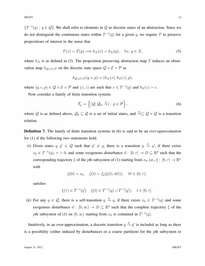
{T−1(q) : q ∈ Q}. We shall refer to elements in Q as discrete states of an abstraction. Since we

do not distinguish the continuous states within T−1(q) for a given q, we require T to preserve

propositions of interest in the sense that

T (x) = T (y) =⇒ hX(x) = hX(y), ∀x, y ∈ X, (5)

where hX is as defined in (3). The proposition preserving abstraction map T induces an obser-

vation map hQ×E×P on the discrete state space Q× E × P as

hQ×E×P(q, e, p) = (hX(x), hZ(z), p),

where (q, e, p) ∈ Q× E × P and (x, z) are such that x ∈ T−1(q) and hZ(z) = e.

Now consider a family of finite transition systems

Tq :={

(Q,Q0,p→) : p ∈ P

}, (6)

where Q is as defined above, Q0 ⊆ Q is a set of initial states, andp→⊆ Q×Q is a transition

relation.

Definition 7. The family of finite transition systems in (6) is said to be an over-approximation

for (1) if the following two statements hold.

(i) Given states q, q′ ∈ Q such that q′ 6= q, there is a transition qp→ q′, if there exists

x0 ∈ T−1(q), τ > 0, and some exogenous disturbance d : [0, τ ] → D ⊆ Rd such that the

corresponding trajectory ξ of the pth subsystem of (1) starting from x0, i.e., ξ : [0, τ ]→ Rn

with

ξ(0) = x0, ξ(t) = fp(ξ(t), d(t)), ∀t ∈ (0, τ),

satisfies

ξ(τ) ∈ T−1(q′) ξ(t) ∈ T−1(q) ∪ T−1(q′), t ∈ [0, τ ].

(ii) For any q ∈ Q, there is a self-transition qp→ q, if there exists x0 ∈ T−1(q) and some

exogenous disturbance d : [0,∞) → D ⊆ Rd such that the complete trajectory ξ of the

pth subsystem of (1) on [0,∞) starting from x0 is contained in T−1(q).

Intuitively, in an over-approximation, a discrete transition qp→ q′ is included as long as there

is a possibility (either induced by disturbances or a coarse partition) for the pth subsystem to


DRAFT 13

implement the transition. In the above definition, time is abstracted out in the sense that we do

not care how much time it takes to reach one discrete state from another.

In Definition 7, if (ii) is not satisfied, i.e., all trajectories of the pth subsystem starting from

T−1(q) leave it eventually, we say that the region T−1(q) or state q is transient for mode p. This

notion of transience can be generalized for a subset of modes in a natural way. A discrete state

q ∈ Q is said to be transient for a subset of modes Ps ⊆ P , if all trajectories of the switched

system (2) starting from T−1(q) leave it eventually under arbitrary switching signals taking

values in Ps. A similar notion of transience is proposed in [4] in the context of autonomous

piecewise multi-affine system. Here we define it for switched system with possible exogenous

disturbances and extend it to ensure progress under switching among a certain set of modes,

which is particularly important when reasoning about the interactions of the system with the

environment at the discrete level.

The following result uses a barrier certificate [36] type condition for verifying a discrete state

being transient.

Proposition 1. Given q ∈ Q and assume that T−1(q) is bounded. The discrete state q is transient

on a family of modes Ps ⊆ P , if there exists a C1 function B : Rn → R and ε > 0 such that

∂B

∂x(x)fp(x, d) ≤ −ε, ∀x ∈ T−1(q), ∀p ∈ Ps, ∀d ∈ D. (7)

Proof: Assume, for the sake of contradiction, that there exists some x0 ∈ T−1(q) and a

switching signal σs taking values in Ps such that the complete trajectory ξ of (2) on [0,∞)

starting from x0 is contained in T−1(q). Condition ((7)) implies that

dB(ξ(t))

dt=∂B

∂x(ξ(t))fσs(t)(ξ(t)) ≤ −ε, (8)

since ξ(t) ∈ T−1(q) and σs(t) ∈ Ps for all t ≥ 0. Integrating this equation would imply

limt→∞B(ξ(t)) = −∞. Yet this leads to a contradiction, as B(ξ(t)) should be bounded if ξ(t)

remains in the bounded set T−1(q).

Next, we provide pseudocode for an algorithm for computing finite-approximations of (1).

We focus on a particularly useful case where T−1(q) are convex polytopes for all q. The main

subroutines of the algorithm are as follows:

• Neighbors(T−1(qj)): returns neighbors of the polytope T−1(qj), i.e., polytopes that share a

common facet with T−1(qj);


DRAFT 14

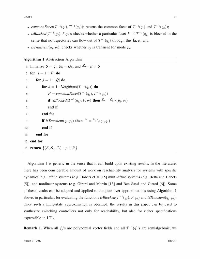
• commonFacet(T−1(qj), T−1(qk)): returns the common facet of T−1(qj) and T−1(qk));

• isBlocked(T−1(qj), F, pi): checks whether a particular facet F of T−1(qj) is blocked in the

sense that no trajectories can flow out of T−1(qj) through this facet; and

• isTransient(qj, pi): checks whether qj is transient for mode pi.

Algorithm 1 Abstraction Algorithm

1: Initialize S = Q, S0 = Q0, andp→= S × S

2: for i = 1 : |P| do

3: for j = 1 : |Q| do

4: for k = 1 : Neighbors(T−1(qj)) do

5: F = commonFacet(T−1(qj), T−1(qk))

6: if isBlocked(T−1(qj), F, pi) then pi→=pi→ \(qj, qk)

7: end if

8: end for

9: if isTransient(qj, pi) then pi→=pi→ \(qj, qj)

10: end if

11: end for

12: end for

13: return{

(S,S0,p→) : p ∈ P

}

Algorithm 1 is generic in the sense that it can build upon existing results. In the literature,

there has been considerable amount of work on reachability analysis for systems with specific

dynamics, e.g., affine systems (e.g. Habets et al [15] multi-affine systems (e.g. Belta and Habets

[5]), and nonlinear systems (e.g. Girard and Martin [13] and Ben Sassi and Girard [6]). Some

of these results can be adapted and applied to compute over-approximations using Algorithm 1

above, in particular, for evaluating the functions isBlocked(T−1(qj), F, pi) and isTransient(qj, pi).

Once such a finite-state approximation is obtained, the results in this paper can be used to

synthesize switching controllers not only for reachability, but also for richer specifications

expressible in LTL.

Remark 1. When all fp’s are polynomial vector fields and all T−1(q)’s are semialgebraic, we


DRAFT 15

can use sum-of-squares-based convex optimization to search for a function B satisfying the

conditions of Proposition 1 in a principled and efficient way. This will provide computationally

efficient means for evaluating isTransient(qj, pi) in Algorithm 1. Similar techniques can be

used to find certificates for isBlocked(T−1(qj), F, pi).

B. Product transition system

Given an over-approximation Tq ={

(Q,Q0,p→) : p ∈ P

}for the switched system (2) and

an environment transition system Te = (E , E0,→) for its environment, we can define a product

transition system for describing the overall system behavior.

Definition 8. The product transition system is a finite transition system Ts := (S,S0,→) with

states in S = Q× E × P , initial states S0 = Q0 × E0 × P0, and transition relation →⊆ S × S

such that (q, e, p)→ (q′, e′, p′) if and only if either e = e′ and qp→ q′, or q = q′ and e→ e′.

It is evident from the definition that Ts consists of two parts: Tq represents the plant dynamics

under switching and Te represents environment changes. Here we consider the product transition

system with interleaving semantics. That is, at each time instant, either the environment state

e or the plant state q changes but they do not change simultaneously1. Defining the product

transition system in an asynchronous way allows the switching mode to react in real time (in

a continuous-time implementation) to environment changes. The price paid is the possibility of

the undesired behavior that the environment Te can make infinitely many transitions before Tqcan make a transition and vice versa. However, as we assume environment signals are of finite

variability, infinitely many transitions of the environment will require an infinite amount of time.

On the other hand, due to underlying dynamics (1), we may show that certain states are transient

under certain sets of modes, that is, the system cannot stay in that state indefinitely if we only

switch within this given set of modes. Hence, the controller can ensure progress in a state, q, by

restricting the modes to those on which q is transient. To encode such transience properties of

a discrete state, we can augment the product transition system with some liveness assumptions

expressible in LTL\©.

1It is possible to consider a truly asynchronous execution to allow such behavior and the results extend to that case trivially.


DRAFT 16

Proposition 2. If state q is transient on the family of modes Ps ⊆ P , then the following LTL\©

property is satisfied

ϕq := ¬ ��((∨p∈Ps

p) ∧ q). (9)

Proof: It is clear from the semantics of LTL that formula (9) implies that the system cannot

remain in mode q forever, if the mode remains within the set Ps, which is the definition of

transience.

Based on the product transition system Ts augmented with the liveness assumption ϕq in (9),

we formulate the following discrete synthesis problem.

Discrete Switching Synthesis Problem: Given a product transition system Ts and the speci-

fication

ϕ := ((ϕq ∧ ϕe)→ ϕs), (10)

synthesize a (discrete) switching strategy that generates only correct executions in the sense that

all executions satisfy ϕ.

It will be shown that, by construction, our solution to the discrete synthesis problem can be

continuously implemented to generate a solution for the continuous switching synthesis problem.

V. DISCRETE SYNTHESIS AS A TWO-PLAYER GAME

In this section, we propose a two-player temporal logic game approach to the discrete switch-

ing synthesis problem formulated in the previous section. In particular, we recast the discrete

synthesis problem as an infinite horizon game. We will first introduce the elements of the game

structure.

A. Game formulation

We consider two-player games, where, at each turn, a move of player 1 is followed by a move

of player 2. We treat player 1 as adversarial, which tries to falsify the specification, whereas

player 2 tries to satisfy it. Formally, a game is defined as follows.

Definition 9. [7] A game structure is a tuple

G = 〈V ,X ,Y , θe, θs, ρe, ρs, ϕ〉,

where


DRAFT 17

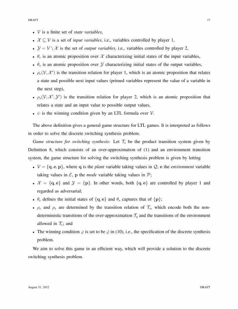
• V is a finite set of state variables,

• X ⊆ V is a set of input variables, i.e., variables controlled by player 1,

• Y = V \ X is the set of output variables, i.e., variables controlled by player 2,

• θe is an atomic proposition over X characterizing initial states of the input variables,

• θs is an atomic proposition over Y characterizing initial states of the output variables,

• ρe(V ,X ′) is the transition relation for player 1, which is an atomic proposition that relates

a state and possible next input values (primed variables represent the value of a variable in

the next step),

• ρs(V ,X ′,Y ′) is the transition relation for player 2, which is an atomic proposition that

relates a state and an input value to possible output values,

• ψ is the winning condition given by an LTL formula over V .

The above definition gives a general game structure for LTL games. It is interpreted as follows

in order to solve the discrete switching synthesis problem.

Game structure for switching synthesis: Let Ts be the product transition system given by

Definition 8, which consists of an over-approximation of (1) and an environment transition

system, the game structure for solving the switching synthesis problem is given by letting

• V = {q, e,p}, where q is the plant variable taking values in Q, e the environment variable

taking values in E , p the mode variable taking values in P;

• X = {q, e} and Y = {p}. In other words, both {q, e} are controlled by player 1 and

regarded as adversarial;

• θe defines the initial states of {q, e} and θs captures that of {p};

• ρe and ρs are determined by the transition relation of Ts, which encode both the non-

deterministic transitions of the over-approximation Tq and the transitions of the environment

allowed in Te; and

• The winning condition ϕ is set to be ϕ in (10), i.e., the specification of the discrete synthesis

problem.

We aim to solve this game in an efficient way, which will provide a solution to the discrete

switching synthesis problem.


DRAFT 18

B. Switching synthesis by game solving

While automatic synthesis of digital designs from general LTL specifications is one of the

most challenging problems in computer science [7], for specifications in the form of the so-

called Generalized Reactivity 1, or simply GR(1), formulas, it has been shown that checking its

realizability and synthesizing the corresponding automaton can be accomplished in polynomial

time in the number of states of the reactive system [7], [32].

GR(1) game: A game structure defined in Definition 9 is a GR(1) game if the winning

condition of the game structure is of the assume-guarantee form ϕ := (ϕe → ϕs) and, for

α ∈ {e, s}, ϕα is of the form

ϕα :=∧i∈Iα1

�ϕα1,i ∧∧i∈Iα2

�♦ϕα2,i, (11)

where ϕα1,i are propositional formulas characterizing safe, allowable moves, and invariants; and

ϕα2,i are propositional formulas characterizing states that should be attained infinitely often. Many

interesting temporal specifications can be transformed into GR(1) specifications of the form (11).

The readers can refer to [7], [32] for more precise treatment on how to use GR(1) game to solve

LTL synthesis in many interesting cases (see also [44] for more examples).

Switching synthesis as a GR(1) game: Recall the assume-guarantee specification for the

discrete synthesis problem:

ϕ := ((ϕq ∧ ϕe)→ ϕs), (12)

where ϕq is the liveness assumption in (9) encoding the transience properties in the product

transition system Ts, ϕe specifies a prior knowledge about the allowable environment behavior

(beyond what is represented by the environment transition system), and ϕs describes the correct

behavior of the overall system. While the liveness assumption ϕq is already of the form (11),

we assume that, for α ∈ {e, s}, each ϕα in (12) also has the structure in (11). Thus, we obtain

a GR(1) game formulation for the switching synthesis problem, which can be solved efficiently.

Winning strategy: A winning strategy for the system (player 2) is a partial function

(s0s1 · · · st−1, (qt, et)) 7→ pt,

which chooses a switching mode based on the state sequence so far and the current moves of

the environment and the plant such that formula (12) is satisfied. We say that ϕ is realizable

if such a winning strategy exists. In addition, for two player LTL games, there always exists


DRAFT 19

finite memory strategies that can be represented by finite automata. Thus, if the specification

is realizable, solving the two-player game gives a finite automaton that encodes the winning

strategy. A feedback switching protocol can be readily extracted from this winning automaton.

More specifically, a mode switch by p is triggered only by a change of state of either q or e. If

there is no change in the environment, following a specific mode, the system will eventually go

to a number of possible states that are allowed by the over-approximation. If there is a change in

the environment, the system is allowed to react to this change immediately, i.e. without waiting

until q changes its state. Thus, by observing both the plant and environment states, the next

switching mode can always be chosen accordingly by reading the finite automaton. Fig. 2 shows

a typical automaton given by solving a two-player game and how it is interpreted as a switching

strategy for the system.

6;q: 2, e: 1, p: 3

14;q: 11, e: 1, p: 3

13;q: 2, e: 2, p: 2

15;q: 5, e: 1, p: 1

17;q: 8, e: 2, p: 4

Fig. 2: Part of a synthesized automaton that can be used to extract a switching strategy. Suppose that the system

arrives at state number 6, where q = 2 and e = 1. It chooses mode p = 3 according to the automaton. Following this

mode, if the environment does not change, i.e. e = 1 is maintained, the system may end up at two different states

q = 11 and q = 5 after a certain period of time, due to non-deterministic state transitions in the over-approximation.

If the environment changes to e = 2 before q changes, the system can react accordingly by possibly switching to

a different mode (in this case p = 2). Following the mode p = 2, if e does not change, the system will end up in

state number 17, where q = 8 and e = 2 and the system will switch to p = 4.

Remark 2. Given a two-player game structure and a GR(1) specification, the digital design

synthesis tool implemented in JTLV [35] (a framework for developing temporal verification


DRAFT 20

algorithm [7], [32]) generates a finite automaton that represents a switching strategy for the

system. The Temporal Logic Planning (TuLiP) Toolbox, a collection of Python-based code for

automatic synthesis of correct-by-construction embedded control software as discussed in [42]

provides an interface to JTLV, which has been used for other applications [30], [31], [42], [43]

and is also used to solve the examples later in this paper.

Remark 3. If there is no external environment and the over-approximation computed for (1), e.g.,

using Algorithm 1, happens to be deterministic in the sense that each of the transition systems

in (6) is deterministic, the game synthesis problem reduces to a model checking problem [25].

In this sense, the temporal game approach outlined in this section covers model-checking based

methods for controller synthesis as a special case [4], [11], [14], [19], [37]. There are certain

trade-offs among computational complexity, conservatism in models and approximations, and

expressivity of specifications, which may make one approach preferable to the other. On the one

hand, model checking is amenable to highly-optimized software [10], [17], with computational

complexity that is linear in the size of the state space [3], but it requires an approximation

that needs to be deterministically implemented for all allowable exogenous disturbances. Such

approximations are potentially difficult to obtain, in the sense that one may not be able to establish

a sufficient number of (deterministic) transitions to make the problem solvable. On the other hand,

over-approximations account for mismatch between the continuous model and its approximation

as adversarial uncertainty and model it nondeterministically. Sufficient approximations of this

type are potentially easier to establish and also allow us to further incorporate environmental

adversaries, yet the resulting formulation is a two-player temporal logic game.

VI. CONTINUOUS IMPLEMENTATIONS OF REACTIVE SWITCHING PROTOCOLS

As discussed in the previous section, a (discrete) switching strategy, represented as a finite

automaton, solves the discrete switching synthesis problem. In this section, we show that we

can implement the (discrete) switching strategy at the continuous level, to provide to a solution

to the continuous switching synthesis problem we posed in Section III.

We define continuous implementations of executions of the product transition as follows. Let

ρ be an execution of Ts, i.e., an infinite sequence of triplets

ρ = (q, e, p) = (q0, e0, p0)(q1, e1, p1)(q2, e2, p2) · · · ,


DRAFT 21

and s = (x, ζ, σ) a trajectory of the switched system (2) and its environment.

Definition 10. The trajectory s is said to be a continuous implementation of ρ, if there exists a

sequence of non-overlapping intervals I = I1, I2, · · · such that ∪∞i=1 = R+ and

x(t) ∈ T−1(qk), ζ(t) = ek, σ(t) = pk, ∀t ∈ Ik, ∀k ≥ 1.

Furthermore, if l(Ik) → ∞ as k → ∞, where l(Ik) denotes the left end-point of Ik, the

implementation is said to be non-Zeno.

Lemma 1. Let ϕ be an LTL\© formula. If s is a non-Zeno implementation of ρ, then

s � ϕ if and only if ρ � ϕ. (13)

Proof: The implementation is non-Zeno guarantees that s produces a well-defined word, say

ws. Let wρ be the word produced by ρ. We can easily show that ws and wρ are stutter-equivalent

[3, Definition 7.86]. Therefore, we have ws � ϕ if and only if wρ � ϕ [3, Theorem 7.92]. The

statement (13) follows by definition.

In this subsection, we show that every continuous implementation of the discrete strategy is

provably correct in the sense that it only generates trajectories satisfying the given LTL specifica-

tion, due to the way we construct the discrete abstraction of the continuous-time switched systems

and solve the discrete synthesis problem. By exploiting properties of an over-approximation, we

can show the following result.

Theorem 1. Given an over-approximation of (1), continuous implementations of the switching

strategy obtained by solving a two-player game solve the continuous switching synthesis problem,

if these implementations are non-Zeno.

Proof: By definition, the switching strategy given by solving a two-player game is a

finite automaton that represents the winning switching strategy for the system. The automaton

provides a switching mode for all possible moves of the environment and the plant. In view of

Proposition 1, the theorem is proved, if we show that the switching strategy generates trajectories

that continuously implement some execution, say ρ = (q, e, p), of the winning automata. The

semantics of the above switching strategy, applied to the switched system (2), are as follows.

Given any initial state x(0) ∈ T−1(q0) and an initial observation of the environment e0, we


DRAFT 22

choose σ(0) = p0, by reading the automaton. From this point on, x(t) evolves continuously

following the dynamics of x = fp0(x, d) (subject to possible exogenous disturbances denoted by

d). Environment signals are monitored in real time. If a change in environment is detected and this

change does not violate the environment assumption, we update the switching mode immediately

according to the automaton. If no environment changes are detected, by the definition of an over-

approximation, there are two possibilities. First, x(t) could stay in T−1(q0) for all t ≥ 0. In this

case, we must have a self-transition in q for this particular mode. The sequence of intervals in

Definition 10 can be chosen arbitrarily as long as they are non-overlapping (Zenoness can also

be avoided by choosing the intervals that l(Ik)→∞ as k →∞). Second, there may exist some

interval I1 (before environment changes its states) and q1 ∈ Q such that x(t) ∈ T−1(q0) for all

t ∈ I1, and either (i) x(τ + ε) ∈ T−1(q1) for all sufficiently small ε > 0 and τ ∈ I1; or (ii)

x(τ) ∈ T−1(q1) and τ 6∈ I1, where τ is a right end-point of I1. In other words, the discrete

state make a transition from q0 to q1 (while environment state remains the same). In either case,

we can choose the next mode from the automata, by observing the evolution of the trajectory

(among the two possibilities above). Note that even if an environment change is detected at

the same time when x(t) enters q1 (although ruled out in our definition of product transition

systems), we can update p in two separate steps. Once a next mode is generated, we repeat the

same procedure as above. It is clear that the trajectory x(t) generated this way implements one

discrete execution of the winning automata.

A. Discussions on non-Zeno implementations

We discuss in this subsection the possibility of Zeno behavior in the continuous implemen-

tations of a discrete strategy and propose appropriate assumptions to exclude such behavior. As

discussed in Section V-B, a switching strategy given by solving a two-player game is a finite-

state automaton. Each continuous implementation of the switching strategy correspond to an

execution of this finite-state automaton, which is an infinite sequence of discrete states of the

form (q, e, p).

Let M be a synthesized automaton. Consider simple cycles in M, i.e., directed paths in M

that start and end with the same state and no other repeated states in between. Let {α1, · · · , αm}

denote the collection of simple cycles inM which include at least two states whose q-components

are different, i.e., triplets (q1, e1, p1) and (q2, e2, p2) with q1 6= q2. For each αj , j = 1, · · · ,m,


DRAFT 23

we can enumerate its states as{

(qji , eji , p

ji ) : i = 1, · · · , lj

}, where lj is the length of the cycle

αj , and consider the set{qj1, · · · , q

jlj

}.

The following proposition can be used to rule out Zeno implementation of the strategy encoded

in M.

Proposition 3. Iflj⋂i=1

T−1(qji ) = ∅, (14)

holds for j = 1, · · · ,m, and the environment signals are of finite variability, then all continuous

implementations of the switching strategy given by M are non-Zeno.

Proof: Note that a Zeno implementation ofM requires visiting an infinite number of discrete

states within a finite time. This means that the trajectory should visit at least one simple cycle

infinitely many times within a finite time. If the environment is of finite variability, this simple

cycle should include at least two states with different q-components. Condition (14) excludes the

possibility of visiting this simple cycle infinitely many times within a finite time (as completing

one cycle would require a definite amount time).

Remark 4. Since T−1(q)∩T−1(q′) = ∅ for q 6= q′, the above emptiness criterion is essentially on

the boundaries of the cells T−1(qji ). Furthermore, if we can check that trajectories implementing

the discrete transitions can only exit within a subset of the boundaries, such as the so-called

exit set in [15], the above emptiness criterion for non-Zenoness can be checked for subsets of

the partitions T−1(qji ), which give more relaxed assumptions than (14). We also remark that

even if the assumption is not satisfied for all possible executions of a given M, Zenoness

can still be avoided at the discrete level by recomputing abstractions such that the assumption

holds, or by adding appropriate specifications to rule out executions whose periodic part can

violate (14). Particularly, since the discrete states in the periodic part typically correspond to

liveness specifications, by appropriately designing abstraction and specifying liveness properties,

Zenoness can be avoided.


DRAFT 24

VII. EXAMPLES

A. Temperature control

Consider a thermostat system [18] with four modes, ON, OFF, Heating, Cooling, as shown

in Fig. 3, where the heating and cooling modes are included to capture what happens while

the heater is heating up to a desired temperature and cooling down to an allowable temperature,

respectively. The dynamics of the four modes are also shown in Fig. 3, where x denotes the room

temperature and y the temperature of the heater. In the OFF mode, the temperature changes at a

rate proportional to the difference between the room temperature x and the outside temperature,

which is equal to 16 in this case, according to Newton’s law of cooling. In other modes, the

change is at a rate proportional to the difference between the room temperature x and the

temperature y of the heater. In the ON mode, the temperature of the heater is kept constant. In

the heating mode, the temperature of the heater increases to 22 at a rate 0.1 per second; in the

heating mode, the temperature of the heater decreases to 20 at a rate 0.1 per second.

We want the system to satisfy the following specifications:

(P1) Starting from any room temperature x and heater temperature y, the system has to reach

a room temperature between 18 and 20 and a heat temperature between 20 and 22, i.e.,

♦(18 ≤ x ≤ 20 ∧ 20 ≤ y ≤ 22).

(P2) If the room and heater temperatures are already in the desired range, they should stay so

for all future time, i.e., the following requirement is enforced

�((18 ≤ x ≤ 20 ∧ 20 ≤ y ≤ 22)→ �(18 ≤ x ≤ 20 ∧ 20 ≤ y ≤ 22)

).

(P3) Transitions among the different modes have to be in the order shown in Fig. 3.

The specification consists of a reachability property and an invariance property in the (x, y)-

plane, together with a sequential constraint in the modes. We start with the synthesis of a

switching strategy that guarantees the reachability property. To obtain a proposition preserving

abstraction, we partition the plane into 12 regions as shown in Fig. 4. The abstraction consists

of plant variable q, whose states belong to Q = {q1, · · · , q12}, and a mode variable p, which

takes values in P = {N, F, H, C}, which represent the ON, OFF, Heating, and Cooling modes,

respectively. By determining the transition relations among the regions in each mode, we obtain

an over-approximation of the system in the sense of Definition 7.


DRAFT 25

x = ‒ 0.002 (x-16).

y = 0.

OFF Heating

Cooling ON

x = ‒ 0.002 (x ‒ y).

y = 0.1.

x = ‒ 0.002 (x ‒ y).

y = 0.x = ‒ 0.002 (x ‒ y)y = ‒ 0.1

.

.

Fig. 3: A four-mode thermostat system.

q1 q2

q3

q4

q5

q6

q7 q8

q9 q10

q11 q12

y=18 y=20 y=22

x=18

x=20

y

x

Fig. 4: A partition of the (x, y)-plane for the thermostat system for synthesizing a switching protocol that guarantees

that the system reaches the region q2.

To synthesize a switching protocol that realizes the reachability ♦(q2), we solve a two-player

game as introduced in Section V-B. The switching protocol can be extracted from a finite

automaton with 32 state.

We then consider the synthesis of a switching protocol that guarantees the invariance property,

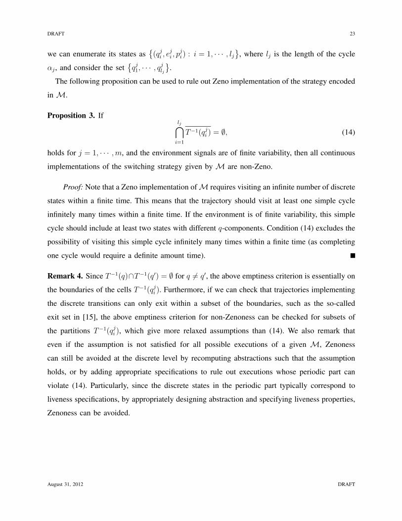
i.e., q2 → �q2. For this purpose, we further partition q2 into six subregions as shown in Fig. 5.

We again obtain an over-approximation and solve a two-player game. The winning protocol can

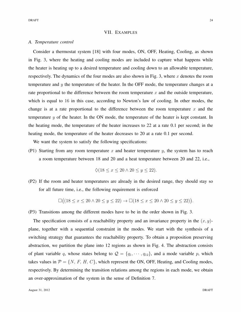
be extracted from a finite automaton with 8 states. A simulation result illustrating a continuous

implementation of this protocol is shown in Fig. 6.


DRAFT 26

20 20.5 21 21.5 2218

18.5

19

19.5

20

y

x

Fig. 5: A further partition of the region q2 (indicated by the red square) in Fig. 4 for synthesizing a switching

protocol that achieves invariance within the region q2.

0 500 1000 1500 2000 2500 3000 3500 4000 4500 500018

18.5

19

19.5

20

20.5

21

21.5

22

t (sec)

[x y]

(cel

sius)

Fig. 6: A simulation illustrating the continuous implementation of a switching protocol that guarantees the

invariance property �(18 ≤ x ≤ 20 ∧ 20 ≤ y ≤ 22): the red line represents the temperature of the heater

and blue line indicates the room temperature.

B. Automatic transmission

Consider a 3-gear automatic transmission system [18] shown in Fig. 7. The longitudinal

position of the car and its velocity are denoted by θ and ω, respectively. The transmission

model has three different gears. For simplicity, the throttle position, denoted by u, takes value

1 in accelerating mode and −1 in decelerating modes. The specification concerns the efficiency


DRAFT 27

of the automatic transmission and we use the functions

ηi(ω) = 0.99 exp

(−(ω − ai)2

64

)+ 0.01

to model the efficiency of gears i = 1, 2, 3, where a1 = 10, a2 = 20, a3 = 30, as similarly

considered in [18]. The acceleration in mode i is given by the product of the throttle and

transmission efficiency.

Let ζ be an environment signal taking value in {1, 2}. The switching synthesis problem is

to find a gear switching strategy to maintain a certain level of transmission efficiency when the

speed is above certain value, while being reactive to the environment signal ζ . Formally, we

consider a specification

�(ω ≥ 5→ η ≥ 0.5) ∧ (0 ≤ ω ≤ 40),

which consists of a minimum efficiency of 50% when the speed is greater than 5, and a speed limit

of 40. In addition, the switching protocol is required to react to the continuous-time environment

signal ζ by switching to a decelerating mode if ζ = 2 and ω ≥ 20, i.e.,

�((ω ≥ 20 ∧ ζ = 2)→ (p = 2 ∨ p = 4 ∨ p = 6)).

θ = ωω = η1(ω)u

..

GEAR = 1


..

GEAR = 2


..

GEAR = 3

Fig. 7: A 3-gear automatic transmission.

Since the properties of interest here are related to ω only, we partition the ω-axis into a

union of intervals Q that preserves the proposition on efficiency. The abstraction consists of

a plant variable q, which takes values in Q, and a mode variable p, which takes values in

P = {±1,±2,±3}. Here, ± denotes accelerating modes and decelerating modes, respectively.

According to this abstraction, we have a deterministic transition system for each of the 7 modes.

The switching synthesis problem can be solved by using the procedure outlined in Section V-B.

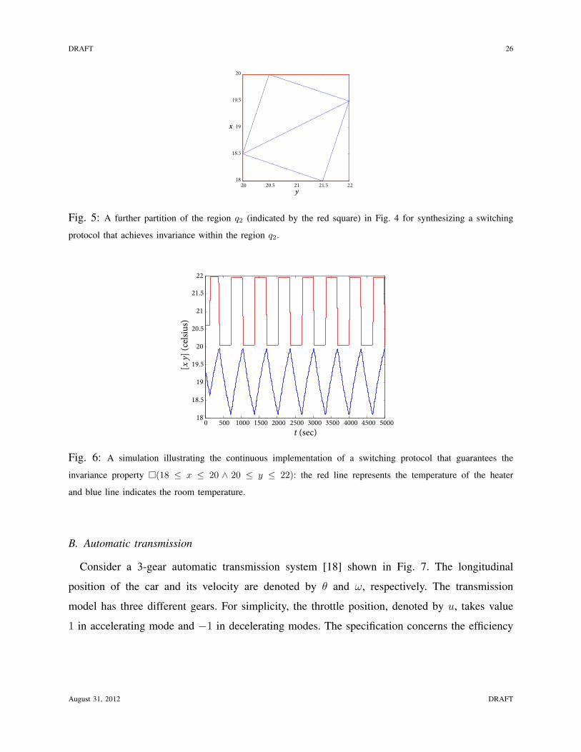
The resulting switching controller can be represented by a finite automaton with 46 states. A

simulation result is shown in Fig. 8, illustrating a continuous implementation of this strategy.

The runtime reactiveness of the switching protocol is evident from the simulation.


DRAFT 28

0 100 200 300 400 500 6000

10

20

30

40

1

2

ω(t)ζ(t)

0 100 200 300 400 500 6000.2

0.4

0.6

0.8

1

η(t)η=5

t (sec)

t (sec)

Effic

ienc

ySp

eed

Envi

ronm

ent

Fig. 8: Simulation results for Example 2: the upper figure shows the speed (ω) and environment (ζ) vs. time, while

the lower figure shows the real-time efficiency (η) of the transmission, where the specified level 50% is indicated

by the red line. It is evident from the upper figure that the system immediately switches to a decelerating mode if

(ω ≥ 20) ∧ (ζ = 2) is satisfied.

C. Robot motion planning

Consider a kinematic model of a unicycle-type wheeled mobile robot [39] in 2D plane:x

y

θ

=

cos θ 0

sin θ 0

0 1

vw

. (15)

Here, x, y are the coordinates of the middle point between the driving wheels; θ is the heading

angle of the vehicle relative to the x-axis of the coordinate system; v and w are the control

inputs, which are the linear and angular velocity, respectively.

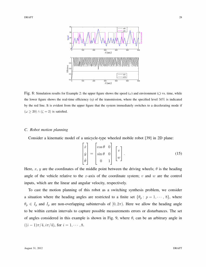
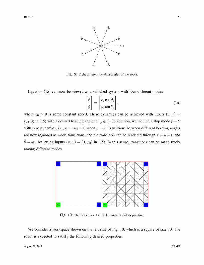
To cast the motion planning of this robot as a switching synthesis problem, we consider

a situation where the heading angles are restricted to a finite set {θp : p = 1, · · · , 8}, where

θp ∈ Ip and Ip are non-overlapping subintervals of [0, 2π). Here we allow the heading angle

to be within certain intervals to capture possible measurements errors or disturbances. The set

of angles considered in this example is shown in Fig. 9, where θi can be an arbitrary angle in

((i− 1)π/4, iπ/4), for i = 1, · · · , 8.


DRAFT 29

θ1

θ2θ3

θ4

θ5

θ5 θ5

θ5

θ = 0

Fig. 9: Eight different heading angles of the robot.

Equation (15) can now be viewed as a switched system with four different modesxy

=

v0 cos θp

v0 sin θp

, (16)

where v0 > 0 is some constant speed. These dynamics can be achieved with inputs (v, w) =

(v0, 0) in (15) with a desired heading angle in θp ∈ Ip. In addition, we include a stop mode p = 9

with zero dynamics, i.e., v0 = w0 = 0 when p = 9. Transitions between different heading angles

are now regarded as mode transitions, and the transition can be rendered through x = y = 0 and

θ = ω0, by letting inputs (v, w) = (0, w0) in (15). In this sense, transitions can be made freely

among different modes.

q0

q1 q3

q2 q0

q1 q3

q2

Fig. 10: The workspace for the Example 3 and its partition.

We consider a workspace shown on the left side of Fig. 10, which is a square of size 10. The

robot is expected to satisfy the following desired properties:


DRAFT 30

(P1) Visit each of the blue cells, labeled as q1, q2, and q3, infinitely often, and avoid obstacles.

(P2) Eventually go to the green cell q0 after a PARK signal is received.

(P3) Stop whenever required.

Here, the PARK signal is an environment signal that constrains the behavior of the robot. The

following assumption is made on the PARK signal.

(S1) Infinitely often, PARK signal is not received.

To synthesize a planner for this example, we introduce a partition of the workspace as shown

on the right side of Fig. 10, in which each cell of size 1 is partitioned into two triangles. In each

mode, we can determine the discrete transition relations according to Definition 7 and obtain an

over-approximation of the system. Solving a two-player game as introduced in Section V-B gives

a winning strategy that guarantees that the robot satisfies the given properties (P1)–(P3). Figs.

11 and 12 present simulation results under different situations. In the case of static obstacles

with crossing objects, the resulting finite automaton of the switching protocol has 161 states,

while it has 37628 states in the case of moving obstacles.

Remark 5. As all cells are transient under each of the modes in {1, · · · , 8}, we encode these

transience properties as additional assumptions as justified by Proposition 1. It is noted that,

without these additional assumptions, the specifications in this example turn out to be unrealiz-

able.

D. Numerical example

We consider the polynomial dynamical systemx1

x2

=

−x2 − 1.5x1 − 0.5x31 + u1 + δ1

x1 + u2 + δ2

(17)

where x = (x1, x2) lies in the domain X = [−2, 2]×[−1.5, 3] and the disturbance δ = (δ1, δ2) lies

in [−0.005, 0.005]× [−0.005, 0.005]. The control inputs are given by u = (u1, u2) = Ki(x1, x2),

i ∈ {1, 2, 3, 4}, which are four different state feedback controllers designed for this system,

with two stabilizing it around desired equilibrium points, and the other two providing some

fast dynamics within the region of interest X . In particular, the following controllers are used:

K1(x) = (0,−x22 + 2), K2(x) = (0,−x2), K3(x) = (2, 10), and K4(x) = (−1.5,−10), where


DRAFT 31

Fig. 11: Simulation results for Example 3. The upper figures show simulation results with static obstacles and

possible crossing objects at intersections (marked as yellow regions). The robot is required to stop at intersections

immediately if crossing objects (indicated by black crosses) are present. This requires runtime reactiveness of the

switching protocol as further illustrated in Fig. 12. The lower figures show simulation results with a moving obstacle

that occupies a square of size 2 and rambles horizontally under certain assumptions on its speed. The blue squares

are the regions that the robot has to visit infinitely often. The green square is where the robot should eventually

visit once a PARK signal is received. The obstacles are indicated by red, the trajectories of the robot are depicted

by black curves, and the current positions of the robot are represented by the magenta dots.

K1 renders the point (−0.669, 1.1540) as a locally stable equilibrium point, and K2 renders the

origin as a globally stable equilibrium point. These equilibrium points correspond to two desired

operating conditions. The goal of the switching protocol is to safely steer the system in between

these two. The domain, X , together with regions of interest, are shown on the left side of Fig.

13. Let A1, A2 and A3 correspond to the red, blue and black regions, respectively. Formally, we

would like to find a switching protocol such that the system satisfies the following specification:

(P1) Remain in X and visit the red and blue regions infinitely often, while avoiding the black

region, i.e.,

�X ∧�¬A3 ∧�♦A1 ∧�♦A2.


DRAFT 32

0 10 20 30 40 50 60 70 80 90 1000

1

2

3

tζ

0 10 20 30 40 50 60 70 80 90 100

0

0.5

1

t

h

0 10 20 30 40 50 60 70 80 90 1000

2

4

6

8

t

σ

Fig. 12: Following Fig. 11, this figure shows the runtime reactiveness of the switching signal σ to changes in

the environment for Example 3. Here ζ is an environment signal ζ that indicates presence of crossing objects at

intersections. In addition, h is a signal taking values in {0, 1}, a change in whose value indicates that the robot

enters a different cell (i.e., a change in q). It can be seen that in addition to reacting to changes in q, the switching

signal also reacts immediately to changes in the environment signal ζ, by switching to the stop mode p = 9 in the

presence of crossing objects at intersections (when ζ = 2, 3).

In addition, the switching protocol and the system is required to react to a continuous-time

environment signal ζ taking value in {1, 2} according to the following rules:

(P2.1) When ζ = 1, the switching protocol is required to steer the system to the red region and

stay there, without using the controller K1; and

(P2.2) When ζ = 2, the switching protocol is required to steer the system to the blue region

and stay there, without using the controller K2.

The following assumptions are made on the environment signal ζ:

(S1) ζ takes each of the values in {1, 2} infinitely often; and

(S2) ζ changes its value only when the system is either in the red or blue region.


DRAFT 33

−2 −1.5 −1 −0.5 0 0.5 1 1.5 2−1.5

−1

−0.5

0

0.5

1

1.5

2

2.5

3

−2 −1.5 −1 −0.5 0 0.5 1 1.5 2−1.5

−1

−0.5

0

0.5

1

1.5

2

2.5

3

Fig. 13: The workspace for Example 4 and its partition.

Based on a partition of the workspace as shown on the right side of Fig. 13, an over-

approximation of system (17) can be computed using Algorithm 1 and sum-of-squares-based

techniques as pointed in Remark 1. A switching protocol can be obtained by solving a two-player

game as introduced in Section V-B. The resulting finite automaton that represents the switching

protocol has 55 states. Simulation results, shown in Fig. 14, illustrate continuous implementations

of the switching protocol, as well as its runtime reactiveness to the environment signal ζ .

VIII. CONCLUSIONS

In this paper, we considered the problem of synthesizing switching protocols for nonlinear

hybrid systems subject to exogenous disturbances. These protocols guarantee that the trajectories

of the system satisfy certain high-level specifications expressed in linear temporal logic. We

employed a hierarchical approach where the switching synthesis problem was lifted to discrete

domain through finite-state abstractions. A family of finite-state transition systems, namely over-

approximations, that abstract the behavior of the underlying continuous dynamical system were

introduced. It was shown that the discrete synthesis problem for an over-approximation can

be recast as a two-player temporal logic game and off-the-shelf software can be used to solve

the resulting problem. Existence of solutions to the discrete synthesis problem guarantees the

existence of continuous implementations that are correct by construction.

In contrast to existing work, we achieve runtime reactiveness of the continuous-time switching

controller by explicitly modeling the environment and taking into account possibly asynchronous

interactions between the system dynamics and the environment. We have accomplished this


DRAFT 34

−2 −1.5 −1 −0.5 0 0.5 1 1.5 2−1.5

−1

−0.5

0

0.5

1

1.5

2

2.5

3

−2 −1.5 −1 −0.5 0 0.5 1 1.5 2−1.5

−1

−0.5

0

0.5

1

1.5

2

2.5

3

0 2 4 6 8 10 12 14 16 18 20

0

0.5

1

1.5

2

t

ζ

0 2 4 6 8 10 12 14 16 18 20

0

0.5

1

1.5

2

t

h

0 2 4 6 8 10 12 14 16 18 200

1

2

3

4

t

σ

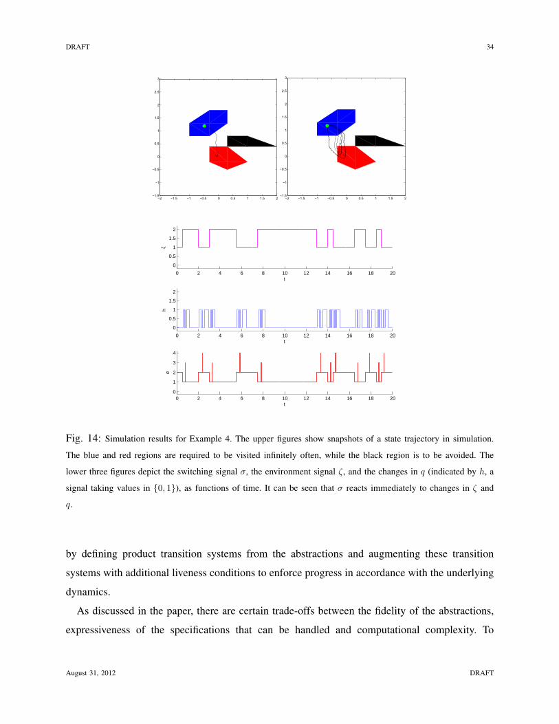
Fig. 14: Simulation results for Example 4. The upper figures show snapshots of a state trajectory in simulation.

The blue and red regions are required to be visited infinitely often, while the black region is to be avoided. The

lower three figures depict the switching signal σ, the environment signal ζ, and the changes in q (indicated by h, a

signal taking values in {0, 1}), as functions of time. It can be seen that σ reacts immediately to changes in ζ and

q.

by defining product transition systems from the abstractions and augmenting these transition

systems with additional liveness conditions to enforce progress in accordance with the underlying

dynamics.

As discussed in the paper, there are certain trade-offs between the fidelity of the abstractions,

expressiveness of the specifications that can be handled and computational complexity. To


DRAFT 35

alleviate the latter issue and to further improve the scalability of the approach, future research

directions include combining the results of this paper with a receding horizon framework and/or

a distributed synthesis approach.

REFERENCES

[1] R. Alur, T. A. Henzinger, G. Lafferriere, and G. J. Pappas, “Discrete abstractions of hybrid systems,” Proc. IEEE, vol. 88,

no. 7, pp. 971–984, 2000.

[2] E. Asarin, O. Bournez, T. Dang, O. Maler, and A. Pnueli, “Effective synthesis of switching controllers for linear systems,”

Proc. IEEE, vol. 88, pp. 1011–1025, 2000.

[3] C. Baier and J. P. Katoen, Principles of Model Checking. MIT Press, 2008.

[4] G. Batt, C. Belta, and R. Weiss, “Temporal logic analysis of gene networks under parameter uncertainty,” IEEE Trans.

Automat. Control, vol. 53, pp. 215–229, 2008.

[5] C. Belta and L. Habets, “Controlling a class of nonlinear systems on rectangles,” IEEE Trans. Automat. Control, vol. 51,

pp. 1749–1759, 2006.

[6] M. A. Ben Sassi and A. Girard, “Computation of polytopic invariants for polynomial dynamical systems using linear

programming,” Automatica, to appear, 2012.

[7] R. Bloem, B. Jobstmann, N. Piterman, A. Pnueli, and Y. Saar, “Synthesis of reactive (1) designs,” J. Comput. System Sci.,

vol. 78, pp. 911–938, 2012.

[8] J. Camara, A. Girard, and G. Gossler, “Synthesis of switching controllers using approximately bisimilar multiscale

abstractions,” in Proc. of HSCC, 2011, pp. 191–200.

[9] A. Church, “Logic, arithmetic and automata,” in Proc. of the ICM, 1962, pp. 23–35.

[10] A. Cimatti, E. M. Clarke, F. Giunchiglia, and M. Roveri, “NUSMV: a new Symbolic Model Verifier,” in Proc. of the

International Conference on Computer Aided Verification, 1999, pp. 495–499.

[11] G. E. Fainekos, H. Kress-Gazit, and G. J. Pappas, “Temporal logic motion planning for mobile robots,” in Proc. of the

IEEE ICRA, 2005, pp. 2020–2025.

[12] E. Frazzoli, M. A. Dahleh, and E. Feron, “Maneuver-based motion planning for nonlinear systems with symmetries,” IEEE

Trans. on Robotics, vol. 21, pp. 1077–1091, 2005.

[13] A. Girard and S. Martin, “Control synthesis for constrained nonlinear systems using hybridization and robust controllers

on simplices,” IEEE Trans. Automat. Control, vol. 57, pp. 1046–1051, 2012.

[14] L. Habets, M. Kloetzer, and C. Belta, “Control of rectangular multi-affine hybrid systems,” in Proc. of the IEEE CDC.

IEEE, 2006, pp. 2619–2624.

[15] L. Habets, P. J. Collins, and J. H. van Schuppen, “Reachability and control synthesis for piecewise-affine hybrid systems

on simplices,” IEEE Trans. Automat. Control, vol. 51, pp. 938–948, 2006.

[16] J. P. Hespanha and A. S. Morse, “Stability of switched systems with average dwell-time,” in Prof. of the IEEE CDC, 1999,

pp. 2655–2660.

[17] G. Holzmann, Spin Model Checker, The Primer and Reference Manual. Addison-Wesley Professional, 2003.

[18] S. Jha, S. Gulwani, S. A. Seshia, and A. Tiwari, “Synthesizing switching logic for safety and dwell-time requirements,”

in Proc. of the International Conference on Cyber-Physical Systems, 2010, pp. 22–31.


DRAFT 36

[19] M. Kloetzer and C. Belta, “A fully automated framework for control of linear systems from temporal logic specifications,”

IEEE Trans. Automat. Control, vol. 53, pp. 287–297, 2008.

[20] M. Kloetzer and C. Belta, “Dealing with nondeterminism in symbolic control,” in Proc. of HSCC. Springer, 2008, pp.

287–300.

[21] T. Koo, G. J. Pappas, and S. S. Sastry, “Mode switching synthesis for reachability specifications,” in Proc. of HSCC.

Springer, 2001, pp. 333–346.

[22] H. Kress-Gazit, G. E. Fainekos, and G. J. Pappas, “Temporal-logic-based reactive mission and motion planning,” IEEE

Trans. on Robotics, vol. 25, pp. 1370–1381, 2009.

[23] J.-W. Lee and G. E. Dullerud, “Joint synthesis of switching and feedback for linear systems in discrete time,” in Proc. of

HSCC, 2011, pp. 201–210.

[24] D. Liberzon and A. S. Morse, “Basic problems in stability and design of switched systems,” IEEE Control Syst. Mag.,

vol. 19, pp. 59–70, 1999.

[25] J. Liu, N. Ozay, U. Topcu, and R. M. Murray, “Switching protocol synthesis for temporal logic specifications,” in Proc.

of ACC, 2012.

[26] O. Maler and D. Nickovic, “Monitoring temporal properties of continuous signals,” in Formal Techniques, Modelling and

Analysis of Timed and Fault-Tolerant Systems. Springer, 2004, pp. 71–76.

[27] Z. Manna and A. Pnueli, The Temporal Logic of Reactive and Concurrent Systems: Specification. Springer, 1992.

[28] T. Moor and J. Davoren, “Robust controller synthesis for hybrid systems using modal logic,” in Proc. of HSCC. Springer,

2001, pp. 433–446.

[29] A. S. Morse, “Supervisory control of families of linear set-point controllers—Part I: Exact matching,” IEEE Trans. Automat.

Control, vol. 41, pp. 1413–1431, 1996.

[30] N. Ozay, U. Topcu, T. Wongpiromsarn, and R. M. Murray, “Distributed synthesis of control protocols for smart camera

networks,” in Proc. of the ACM/IEEE International Conference on Cyber-Physical Systems, 2011.

[31] N. Ozay, U. Topcu, and R. M. Murray, “Distributed power allocation for vehicle management systems,” in Proc. of the

IEEE CDC, 2011.

[32] N. Piterman, A. Pnueli, and Y. Saar, “Synthesis of reactive (1) designs,” in Proc. of the International Conference on

Verification, Model Checking, and Abstract Interpretation, 2006, pp. 364–380.

[33] A. Pnueli, “The temporal logic of programs,” in Proc. of the Annual Symposium on Foundations of Computer Science,

1977, pp. 46–57.

[34] A. Pnueli and R. Rosner, “On the synthesis of an asynchronous reactive module,” in Proc. of the International Colloquium

on Automata, Languages and Programming, 1989, pp. 652–671.

[35] A. Pnueli, Y. Sa’ar, and L. Zuck, “JTLV: A framework for developing verification algorithms,” in Proc. of the

International Conference on Computer Aided Verification, vol. 6174, 2010, pp. 171–174, associated tool available at

http://jtlv.ysaar.net/.

[36] S. Prajna and A. Jadbabaie, “Safety verification of hybrid systems using barrier certificates,” in Proc. of HSCC. Springer,

2004, pp. 271–274.

[37] P. Tabuada and G. J. Pappas, “Model checking LTL over controllable linear systems is decidable,” in Proc. of HSCC.

Springer, 2003, pp. 498–513.

[38] A. Taly and A. Tiwari, “Switching logic synthesis for reachability,” in Proc. of the ACM International Conference on

Embedded Software, 2010, pp. 19–28.


DRAFT 37

[39] J. M. Toibero, F. Roberti, and R. Carelli, “Stable contour-following control of wheeled mobile robots,” Robotica, vol. 27,

pp. 1–12, 2009.

[40] J. Tumova, B. Yordanov, C. Belta, I. Cerna, and J. Barnat, “A symbolic approach to controlling piecewise affine systems,”

in Proc. of the IEEE CDC, 2010, pp. 4230–4235.

[41] G. Weiss and R. Alur, “Automata based interfaces for control and scheduling,” in Proc. of HSCC. Springer, 2007, pp.

601–613.

[42] T. Wongpiromsarn, U. Topcu, N. Ozay, H. Xu, and R. M. Murray, “TuLiP: a software toolbox for receding horizon temporal

logic planning,” in Proc. of HSCC, 2011, pp. 313–314.

[43] T. Wongpiromsarn, U. Topcu, and R. M. Murray, “Formal synthesis of embedded control software: Application to vehicle

management systems,” in Proc. of the AIAA Infotech@Aerospace Conference, 2011.

[44] T. Wongpiromsarn, U. Topcu, and R. M. Murray, “Receding horizon temporal logic planning,” IEEE Trans. Automat.

Control, to appear, 2012.


draft 1 synthesis of reactive switching protocols from...

Documents