
Thomas Mo 1
X-Ray Backlighting of Shock Ignition Experiments on the National Ignition Facility
Thomas Mo
Webster Schroeder High School
LLE Advisor: Dr. R.S. Craxton
Laboratory for Laser Energetics
University of Rochester
Rochester, New York
November, 2010

Thomas Mo 2
Abstract:
A computer code Blackthorn has been written to model the radiography of an imploding
fusion target using an x-ray backlighter. Blackthorn traces x rays from the backlighter source
through the target to a camera, which is at an arbitrary viewing angle. Blackthorn can model
the target at any specified time and x-ray energy, drawing a contour plot that imitates an actual
image produced by an x -ray backlighter, including self-emission, from the perspective of the
viewing position. Input files from a computer code SAGE, which contains a 3D grid of center of
mass radius, are combined with input files from another code, LILAC, which contains 1D profiles
of mass density and electron temperature versus radius, to produce a 3D representation of the
target density. The capabilities of Blackthorn are illustrated by application to a f usion target
proposed for shock-ignition polar-drive experiments on t he National Ignition Facility (NIF). A
view from the polar position can be u sed to diagnose the azimuthal uniformity of the target,
while a view from the equator can be used to diagnose the balance of compression between the
polar and eq uatorial positions. Blackthorn is being used to help design and opt imize x-ray
backlighting diagnostics for the proposed experiments. U sing 1D line-plots created by
Blackthorn, 3500eV has been determined as an optimal frequency to view backlighting images.

Thomas Mo 3
1. Introduction:
Fusion is the process through which two or more nuclei fuse together to form a single
heavier nucleus. Normally, fusion creates a more stable nucleus and results in the release of a
large quantity of energy. To achieve fusion, the nuclei must be at a high density and
temperature. These conditions will increase the number of collisions between the nuclei and
increase their kinetic energy, so
that the nuclei will overcome
their repulsive electrostatic
forces in favor of their attractive
nuclear forces and fuse
together. In hydrogen fusion, a
deuterium nucleus fuses with a
tritium nucleus to create a
helium nucleus and a neutron
with a large amount of energy.
Applying this concept to a
spherical fuel capsule
consisting of a thin plastic shell filled with deuterium and tritium, fusion reactions can be carried
out. These fusion reactions can provide a means of creating a future source of energy. The
conditions for fusion can be met by using high-energy lasers to strike the capsule. The lasers
deposit energy on the outside of the capsule so the outside ablates and the inside implodes. If
the implosion is uniform and the conditions are met, fusion will occur.

Thomas Mo 4
There are two ways to
implode the target with lasers:
indirect drive fusion1 and
direct drive fusion2 (Fig. 1).
Indirect drive fusion involves
laser beams striking the
inside of a hohlraum, a
metallic cylinder through
which the laser beams enter
from the top and bot tom, which then emits x-rays to irradiate the fuel capsule, located at the
center of the cylinder. The National Ignition Facility (NIF) in Livermore, California is built for and
currently specializes in indirect drive experiments. The NIF uses 192 beams of lasers organized
into 48 q uads (set of four lasers), in which all are designed to irradiate the inside of the
holhraum wall from the top and bottom. The quads are located at angles of 23.5, 30, 44.5, and
50 degrees to the z axis above and below the equator. On the other hand, in direct drive fusion,
the laser beams directly and uniformly irradiate the target from all incident angles. Since the NIF
facility has no equatorial beams, as it was constructed primarily for indirect drive experiments,
polar direct drive3,4 has been designed to enable direct drive experiments to be performed on
the NIF. In polar direct drive, the beams maintain their indirect drive port configurations, but are
re-pointed from the center of the target to achieve the best uniformity after compression (Fig. 2).
Currently, there are two main types of direct drive that may provide a path to attaining
fusion energy in the future: hotspot ignition and shock ignition. Hotspot ignition6 consists of the
simultaneous heating and compression of the target center to start fusion in the center. Once
fusion is present in the center, alpha particles (helium nuclei) will propagate outward and heat
the fuel, creating a chain reaction. However, compressing a target full of “hot fuel” is very
difficult, so an alternative technique, called shock ignition, has been proposed (Fig. 3). Shock

Thomas Mo 5
ignition8,9 contains two steps. I n the first step, the “cold fuel” is compressed at low velocity,
represented by the portion of the red curve with lower power (Pmain) in Fig. 3. In the second
step, a powerful laser pulse,
represented by the Pshock portion of
the red curve, is used to launch a
short, strong, spherically
convergent shock on the outside of
the target. The shock propagates
inward, and the focused energy
heats the center rapidly to generate
fusion. Shock ignition can only be
performed with direct drive because
the short laser pulse cannot heat the holhraum to a high enough temperature rapidly enough.
Perkins has proposed to test polar direct drive shock ignition on the NIF7. Half of NIF’s
beams, 96 main beams, are used to form the compression pulse and the other half, the 96
igniter beams, are used to form the shock pulse7. During the first part of the experiment, only the
compression step is proposed to see if the fuel capsule, also referred to as the target, can be
compressed sufficiently and uniformly using only half of the NIF beams. Tucker10 has developed
a design for this compression stage, but since this design and future designs may not produce
perfect uniformity in compression, x-ray backlighting is needed to diagnose the uniformity, which
is vital to achieving fusion. For x-ray backlighting, some laser beams not used to irradiate the
target strike an x-ray source and create a layer of plasma (Fig. 4). The layer of plasma then
emits x-rays which pass through the target, and those rays that pass through the pinhole and
onto the x-ray detector create the backlighting image.

Thomas Mo 6
Unfortunately, NIF
shots are exceedingly
limited; the system is
capable of shooting up to
three times per day, but
presently the NIF only
shoots once per day.
Therefore, simulations of
x-ray backlighting must
be completed before the
actual experiment is
carried out. Tucker’s
design, obtained using
the code SAGE11, can
provide predictions of the 3D target shell, but prior to this work the capability to simulate the x-
ray backlighting image of the 3D object did not exist. This work describes a computer code
Blackthorn that has been written to predict the image seen by an x-ray detector from any
detector angle relative to the capsule.

Thomas Mo 7
2. X-ray Propagation in Blackthorn:
2.1: Theory
For an x ray of frequency v moving along a path whose position is measured by its
distance of travel s, (Fig. 5(a)), its spectral intensity Iv is given by the equation of radiation
transfer12:
(1)
where is the opacity and Bv is the blackbody spectral intensity evaluated at the local
temperature. The first term on the right hand side depends on Iv, where Iv*ds*dΩ*dt*dv equals
the energy crossing a x-ray receiving area ds, dv is the frequency interval of the x ray, dΩ is the

Thomas Mo 8
solid angle, and dt is the time interval. The second term depends on Bv, the blackbody spectral
intensity of the target given by Planck’s law12:
(2)
where h is Planck’s constant, v is the x-ray frequency, c is the speed of light, k is Boltzmann’s
constant, and T is the local temperature. Eq. 2 shows that Bv is only a function of the x-ray
frequency and the local temperature at the x-ray position.
In Eq. (1), the first term represents absorption and the second term represents self-
emission. Since Bv is a function of temperature, if it is assumed that T=0 so that Bv, and
consequently the self-emission term, becomes negligible, Eq. 1 becomes:
(3)
Solving for Iv, Eq. 3 becomes:
(4)
the ideal case of backlighting. In this equation Iv,start is the spectral intensity emitted by the
backlighter source, and the integral of ds is the optical depth. Since is consistently large
inside the target shell and approximately zero outside, the optical depth depends mainly on the
distance of x-ray travel through the shell. Therefore, the optical depth is almost 0 for rays
starting at A, intermediate at B, and large at C (Fig. 5). Unfortunately, the local temperature on
the x-ray path can reach up to several thousand electron volts, causing self-emission to become
a significant factor.
To solve Eq. 1, Iv,start needs to be known. It can be parameterized as a function of the
backlighter temperature TXR:
Thomas Mo 9
Iv,start=Bv(TXR). (5)
Currently, 300 eV has been determined as a reasonable13 backlighter temperature.
2.2: Numerical algorithm for integrating an x-ray path
The x-ray is integrated along its path taking small steps of interval ds. Assuming that the
temperature and opacity are constant on the interval, Eq. 1 can be rewritten as:
(6)
since dBv/ds=0. Integrating each side,
(7)
is obtained. This gives the spectral intensity at the new position:
. (8)
As in Eq. 1, the first term of Eq. 8 on the right hand side represents the absorption while the
second term represents the self-emission. Eq. 8 maintains the assumption that the spectral
emission occurring during an interval of x-ray travel ds is defined by Eq. 2 for the local
temperature and opacity at the beginning of the interval. Since the temperature and opacity can
change quickly, especially when the x-ray is near the shell of the target, a small ds needs to be
used to accommodate this assumption. Convergence is achieved once the ds is small enough
that an image created with a value ds and another image created with a value ½ds are almost
indistinguishable.
3. Solutions for 1-D hydrodynamic profiles:
3.1: Introduction of 1-D hydrodynamic profiles
In order to solve Eq. 8, the opacity and Bv need to be known. For the ideal case of a
spherically symmetric shell, the temperature and density profiles can be obtained from a 1-D
Thomas Mo 10
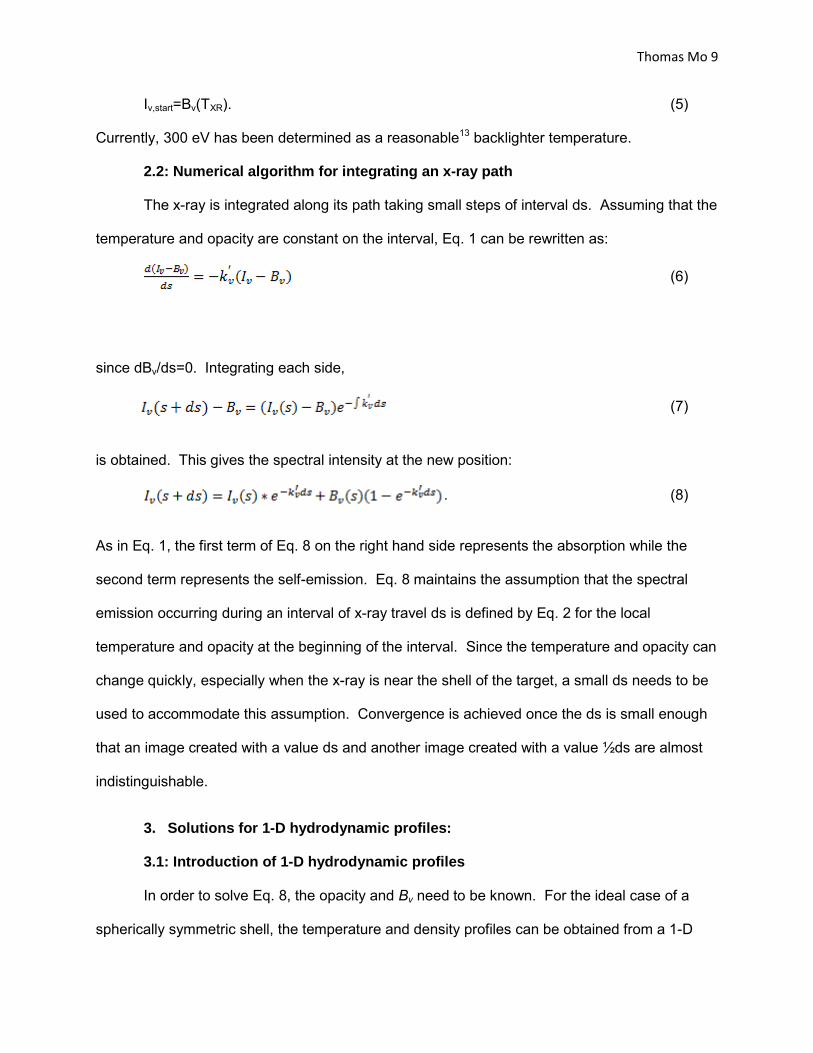
hydrodynamic code such as LILAC. LILAC provides densities and temperatures as a function of
radius R, the distance from the target center (Fig. 6). In Fig. 6, the target shell is between 400
and 500 microns in radius. On the right side of the high density spike, the outside of the shell is
hot from the lasers striking the surface. Inside the shell (left), the DT has a low density, and is
heated by energy from the shock
propagating inwards. Since the
curves of density and
temperature versus radius are
smooth, the density and
temperature of any given radius
can be found using linear
interpolation. One of the
quantities needed to solve Eq. 8
is opacity, . This is provided by
data from the Los Alamos Astrophysical Opacity Library,14 giving opacity as a function of
density, temperature, and frequency. Therefore, for any given x-ray with a known frequency
and radius R, the opacity can be found using interpolation with respect to the density,
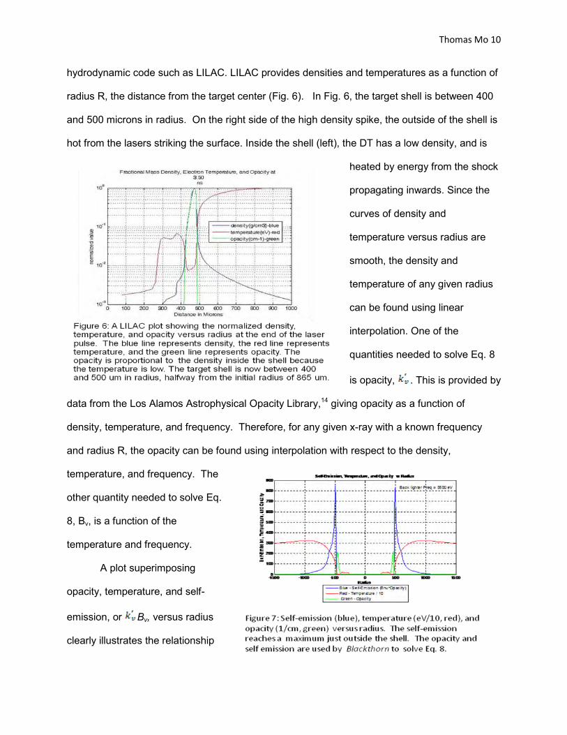
temperature, and frequency. The
other quantity needed to solve Eq.
8, Bv, is a function of the
temperature and frequency.
A plot superimposing
opacity, temperature, and self-
emission, or Bv, versus radius
clearly illustrates the relationship

Thomas Mo 11
between the three values (Fig. 7). The opacity is high for the shell, where the temperature and
self-emission are low. The self-emission reaches a maximum just outside the shell when the
temperature is still moderately high. Self emission drops inside the target because the inside of
the target is cool relative to the hot shell. As the radius increases, the self-emission also
decreases due to a decrease in opacity.
3.2: Predicted backlighting for 1D target profiles
Fig. 8 shows graphs of spectral intensity versus distance s along the x-ray paths B and
C of Fig. 5a, containing superimposed curves of the spectral intensity with and without self-
emission. Figure 8a displays rays passing through the center of the target and Fig. 8b rays
closest to the edge of the target shell. In both cases, the self emission increases the spectral
intensity directly outside the target shell and after it passes completely through the target. Since
the x-ray in Fig. 8b has a longer portion of its path inside the shell, more absorption occurs, and
less intensity emerges from the target.
To predict what experimentalists would see on the backlighting images, Fig. 5b shows
graphs of spectral intensity versus radius in the image plane with and without self-emission. The

Thomas Mo 12
transmission begins to rapidly drop just inside the outer radius of the target shell and reaches a
minimum at the edge of the inner radius of the shell. This allows the backlighting image to
reveal the inside and outside edges of the target. Self-emission increases the spectral intensity
shown on the backlighting image inside the target and creates an increase of the spectral
intensity to values above Iv,start around the outside edge of the target. However, the self-
emission in Fig. 5b does not affect the location of the inner or outer edges of the shell.
3.3: Frequency Optimization
To find an optimal frequency, superimposed plots of transmission versus radius in the
image plane for different x-ray frequencies can be used (Fig. 9). Fig. 9 is similar to Fig. 5b, but
instead of spectral intensity (Iv) ,
the transmission, Iv,final/Iv,start is
plotted. The transmission
depends strongly on the x-ray
frequency.
As the x-ray frequency
increases, the value of the
exponential in Eq. 2 also
increases, and would result in a
lower Bv in the plasma and a
lower Iv,start. This exponential
term changes much more
dramatically for the x-ray source than the plasma, so Iv,start is greatly reduced for higher x-ray
frequencies. In this case, the target becomes dominated by self-emission, as shown by the
curve representing an x-ray frequency of 5000 eV. The minimum transmission inside the target
becomes 3.5, and the maxmimum transmission, caused by the x-rays that are skimming the

Thomas Mo 13
outside of the shell, is more than 8.5. At the other extreme, shown by the curve with an x-ray
frequency of 1500 eV, the transmission inside the shell is consistently close to zero. The shape
of this curve is similar to the transmission curve with no self-emission (red) shown in Fig. 5b.
Having too high or too low of an x-ray frequency is problematic because in both cases
there is a lack of information about the inside of the shell. In the 5000 eV case, the image would
be created primarily by the target’s self emission. On the other hand, for the 1500 eV x-rays,
the x-rays are so strongly attenuated that little energy reaches the inside of the target, so x rays
don’t fully penetrate the target and emerge with sufficient energy to provide details about the
inside. The 3500 eV x-rays create a curve that comes closest to the ideal transmission curve;
the transmission is 1 outside the target (except the regions directly outside the target slightly
affected by self-emission), and the transmission curve reaches a minimum just inside the shell
and increases towards the center, following the limb effect. Therefore, a frequency of 3500 eV
has been temporarily chosen.
3.4: Images taken after
the end of the laser pulse
The backlighting image
can also be taken after the laser
pulse has been turned off. This
can be simulated by using a
temperature factor, wherein all
the temperatures obtained from
the LILAC profile are mutliplied
by this factor in order to mimic
the cooling of the target over

Thomas Mo 14
time after the laser pulse has ended. A 1-D plot of spectral intensity versus radius in the image
plane with superimposed plots with three different temperature factors can be used to analyze
the effects of cooling (Fig. 10). The temperature factors used are 1, 0.5, and 0.2, simulating the
target 0,0.35, and 0.85 nanoseconds after the laser pulse has been shut off. As the temperature
factor decreases, the transmission maxima decrease, signifying that the amount of self-
emission also decreases. Once the temperature factor is as low as 0.2, almost no self-emission
is shown, shown by the flat spectral intensity outside of the target. In addition, a much clearer
minimum just inside the shell can be seen. Therefore, images taken after the laser pulse should
be better than those taken during the pulse. To adjust for this advantage, the laser pulse could
possibly be switched off slightly earlier to obtain self-emission-free images for more times.
4. Modeling of 3D target profiles
Each target position can be represented by a spherical angle (θ,Φ) where θ is the angle
clockwise from the positive z-axis and Φ is the angle clockwise from the x-axis in the x-y plane.
As described by Tucker10, the computer code SAGE calculates the center of mass radii for
positions all around the target as a function of (θ,Φ). Typical plots of the center of mass radii are

Thomas Mo 15
shown in Fig. 11 for Tucker’s initial and final designs. Red areas represent areas that are over-
compressed, while blue areas represent ones that are under-compressed. The darker the color
is, the more over/under compressed the area is. In both (a) and (b), the equatorial positions are
compressed less than the polar positions. However, it is obvious that the initial design shows a
much greater difference in the compression between the polar and equatorial positions.
SAGE produces profiles similar to the LILAC profiles of density and temperature versus
radius, but with less resolution, since SAGE is a 2D code. To compensate for the lower
resolution, a LILAC profile can be
combined with the SAGE center of
mass calculations by shifting the
LILAC profiles in each direction
(θ,Φ) to match the center of mass
provided by SAGE. In the solutions
described above for 1D
hydrodynamic profiles, calculations
were made purely based on LILAC,
where the radius used for
interpolation was the distance R
from the current x-ray position to the center of the target (see Fig. 5a). For 3D targets, with an x
ray at position (R,θ,Φ), Blackthorn first finds the center of mass radius (rcm) in the direction
(θ,Φ), and then calculates a new radius rnew to correspond with the LILAC profile using the
equation:
rnew=(R-rcm)+rmax_density. (9)
where rmax_density is the radius in the LILAC profile corresponding to the maximum density. rnew is
then used to interpolate for density, temperature, and opacity in LILAC. So, for example,

Thomas Mo 16
whenever the x ray radius R is equal to rcm, Eq. 9 will cause the LILAC values to be calculated at
rnew = rmax_density. SAGE records the radii rcm by creating a three-dimensional cube that encloses
the target with grids, usually 20x20 or 30x30, on each of the 6 faces (Figure 12). This method is
described in Ref. 15. At the center of each square on each grid is a grid-point at which the
center of mass radius rcm is stored. When the x ray moves to a new position (x,y,z) for which (R,
θ, Φ) are calculated, Blackthorn finds the coordinates where the red line in the direction (θ, Φ)
intersects one of the grids. Then, Blackthorn calculates rcm in that direction using bilinear
interpolation.
4.1: Selection of rays:
Given a viewing direction (θ,Φ), a unit vector c=(sin(θ)cos(Φ),sin(θ)sin(Φ),cos(θ)) can be
used to represent the direction of the camera and of x-ray travel with respect to the x,y,z axes.
Using the components of the direction vector, an imaginary (u,v) plane, which is perpendicular
to the direction of x-ray travel, can be created. The (u,v) plane is placed 1500 um away from the
target center and simulates the image plane (see Fig. 5a), where x-rays strike and form the
image. The components of unit vectors in the u and v directions can be defined by u1=(-sin(Φ),
cos(Φ), 0) and v1=(-cos(θ)cos(Φ), -cos(θ)sin(Φ), sin(θ)). Given the coordinates of the x-ray
starting position in the (u,v) plane, the unit vectors are used to find the starting coordinates in
the (x, y, z) plane.
Blackthorn shoots rays in a polar fashion from the center of the (u,v) plane. The x-rays
are first shot along the radial direction at angle of 0 with respect to the positive u-axis. This is
repeated for the other angles. Polar ray tracing allows the curves of the contour plot to be
smoother than the jagged curves resulting from a rectangular grid of x-rays. Therefore, it allows
a much smaller number of rays to be used in order to reach convergence.

Thomas Mo 17
5. Predicted images for 3D target profiles
Two different camera angles are available on the NIF for viewing backlighting images. A
view from the
pole position
(θ=0,Φ=0) can
be used to
diagnose the
azimuthal
uniformity of
the target
while a view
from the
equator
(θ=90, Φ=79) can be used to diagnose the balance of compression between the polar and
equatorial positions.
Fig. 13 shows a polar-view backlighting
image of Tucker’s initial design. The x-ray
energy used is 3500 eV and TXR is 300 eV. The
yellow portion shows the outside of the target,
where the transmission is 1. The orange ring
indicates that the transmission is greater than
1, and is caused by self-emission from just

Thomas Mo 18
outside the target’s
shell. The thin black
ring shows the outer
edge of the target’s
shell. Inside the black
ring, the transmission
rapidly transitions from
the higher value outside
the shell to the lower
value inside (Fig. 14).
The image of Fig.13 shows a four-fold nonuniformity pattern around the outside ring of the
target. The offset of the pattern from 0,90,180, and 270 degrees corresponds with the offset of
the beams on the NIF equatorially (see Fig. 11). Slight nonuniformities can also be seen directly

Thomas Mo 19
inside the ring, also in a four-fold pattern. When viewing Tucker’s final design from the polar
view (Fig. 15), the overall shape of the target is much more round. Most of the structure around
the outside of the ring is eliminated. Some structure inside the ring, also in a four-fold pattern,
can just be perceived.
In the equatorial view of Tucker’s original design (Fig. 16a), it is clear that the equatorial
positions are compressed much less than the polar positions. There is also a significant amount
of structure directly inside the shell. In the equatorial view of Tucker’s final design (Fig. 16b),
the nonuniformity is much less, but the equatorial positions are still compressed slightly more.
The inner structure has also been reduced.
Conclusion
A shock-ignition experiment has been propsed for the National Ignition Facility. To
model x-ray backlighting of targets for these experiments, a computer code Blackthorn has
been written. Blackthorn combines a 1-D LILAC profile with 3-D SAGE predictions to create 1-D
plots of x-ray intensity and 2-D backlighting images that can be used to diagnose the uniformity
of target compression. Blackthorn can also help optimize the x-ray frequency, backlighter
temperature TXR, and times to take the backlighting images. The exact TXR will depend on the
number of beams used for backlighting and the material of the backlighting source. Blackthorn
determined that 3500 eV is an optimal frequency to form backlighting images, which should be
taken just after the laser pulse has been turned off to reduce the effects of self-emission.
Blackthorn shows a clear distinction between optimum designs, like Tucker’s design which
produces very spherical images, and non-optimum designs, which produce clearly nonuniform
images, enabling nonuniform implosions to be diagnosed. Blackthorn can thus be used in
support of research on the NIF towards the possibility of obtaining fusion energy using shock-
ignition.

Thomas Mo 20
Acknowledgements:
I would like to thank Dr. Craxton for inviting me to the summer program, taking time to advise
my project, and supporting me during and after the program. I would also like to thank Laura
Tucker for aiding my research with a more optimized capsule design.
References:
1. J.D. Lindl, “Development of the Indirect-Drive Approach to Inertial Confinement Fusion and the Target Physics Basis for Ignition and Gain,” Phys. Plasmas 2, 3933 (1995).
2. J Nuckolls et al., “Laser Compression of Matter to Super-High Densities: Thermonuclear (CTR) Applications,” Nature 239,139 (1972).
3. S. Skupsky et al., “ Polar Direct Drive on the National Ignition Facility “, Phys. Plas 11, 2763 (2004)
4. R.S. Craxton et al., “Polar Direct Drive : Proof-of-Principle Experiments on OMEGA and Prospects for Ignition of the National Ignition Facility,” Phys. Plas 12, 056305 (2005)
5. A.M. Cok, “Development of Polar Drive Designs for Initial NIF targets,” LLE Summer High School Research Program (2006)
6. S. Atzeni and J. Meyer-ter-Vehn, “The Physics of Inertial Fusion,” Clarendon (2004).
7. L.J. Perkins, et al., “Development of a Polar Drive Shock Ignition Platform on the National Ignition Facility,” NIF Facility Time Proposal (2010).
8. R. Betti et al., “Shock Ignition of Thermonuclear Fuel with High Areal Density,” Phys. Rev. Lett. 98, 155001 (2007)
9. L.J. Perkins et al., “Shock Ignition : A New Approach to High Gain Inertial Confinement Fusion on the National Ignition Facility,“Phys. Rev. Lett. 103, 045004 (2009)
10. L. Tucker, “A Design for a Shock Ignition Experiment on the NIF Including 3-D Effects,” LLE Summer High School Research Program (2010)

Thomas Mo 21
11. R.S. Craxton and R.L. McCrory, “Hydrodynamics of Thermal Self-Focusing in Laser Plasmas,” J. Appl. Phys. 56, 108 (1984).
12. Ya. B. Zel'dovich, Yu. P. Raizer, “Physics of Shock Waves and High-Temperature Hydrodynamic Phenomena, ” New York: Academic Press (1966-1967)
13. R. Epstein, Discussion about backlighting temperature, 11 October 2010
14. W.F. Huebner et al., “ Astrophysical Opacity Library, “ Los Alamos Scientific Laboratory Report LA-6769-M (1977)
15. G. Balonek, “How good is the Bright Ring Characterization for Uniformity of Deuterium Ice Layers Within Cryogenic Nuclear Fusion Targets?,” LLE Summer Program (2004)


