> REPLACE THIS LINE WITH YOUR PAPER IDENTIFICATION NUMBER (DOUBLE-CLICK HERE TO EDIT) <
1
Abstract—An effective condition monitoring system of wind
turbines generally requires installation of a high number of
sensors and use of a high sampling frequency in particular for
monitoring of the electrical components within a turbine,
resulting in a large amount of data. This can become a burden
for condition monitoring and fault detection systems. This paper
aims to develop algorithms that will allow a reduced dataset to be
used in wind turbine fault detection. The paper firstly proposes a
variable selection algorithm based on principal component
analysis (PCA) with multiple selection criteria in order to select a
set of variables to target fault signals while still preserving the
variation of data in the original dataset. With the selected
variables, the paper then describes fault detection and
identification algorithms, which can identify faults, determine the
corresponding time and location where the fault occurs, and
estimate its severity. The proposed algorithms are evaluated with
simulation data from PSCAD/EMTDC, SCADA (Supervisory
control and data acquisition) data from an operational wind
farm, and experimental data from a wind turbine test rig. Results
show that the proposed methods can select a reduced set of
variables with minimal information lost whilst detecting faults
efficiently and effectively.
Index Terms— Variable selection, principal component analysis,
fault detection, condition monitoring, wind turbines
I. INTRODUCTION
HE importance of continuous and autonomous condition
monitoring (CM) and fault detection systems for
engineering applications has increased dramatically in the past
decades. This is particularly the case for wind power, as
turbines are often deployed in remote and harsh environments.
CM techniques can help improve the performance and
reliability of the wind turbines (WTs) [1]. According to
IRENA, the operation and maintenance cost of a WT is
between 10% - 25% of the total cost of electricity [2, 3]. With
increasing size and complexity of turbines, and the move to
building more offshore wind farms, maintaining the
performance and reliability of WTs technically and financially
has become a challenge.
Based on the information collected from sensors, a CM
system monitors and identifies potential anomalies and
predicts WT’s future operation trend, allowing preventative
maintenance of the turbine to be undertaken. With a
This work was jointly supported by UK Engineering and Physical Sciences
Research Council (EPSRC) under Grant EP/I037326 and Engineering
Department at Lancaster University.
Y. Wang, X. Ma and P. Qian are all with the Engineering Department at Lancaster University, UK (e-mail: [email protected]).
sufficiently early warning, it is possible to reduce down-time
and avoid component damage due to unexpected failures.
Moreover, by continuous monitoring of the WT’s components,
the life cycle of turbine components can be estimated, and
maintenance activities scheduled accordingly to optimize asset
management.
An effective CM system for wind turbines relies upon
algorithms designed for accurate fault detection and
prediction; however, there are two major issues. The first of
these is associated with the amount of data generated by
sensors. Typically, a wind turbine CM system monitors
approximately 150-250 variables [4], and its sampling rate
depends on the nature of the monitoring system, ranging from
0.002 Hz (e.g. SCADA) to >10 kHz data for dedicated
diagnostic purposes. The need to store and process these data
increases the cost, and complicates the performance of both
the CM system and the interpretation of its output. The second
issue relates specifically to sensor reliability. Elouedi et al.
and Guo et al. have both pointed out issues regarding the
accuracy and accountability of sensors used for pattern
recognition and fault identification and diagnosis [5, 6]. For a
CM system, the accuracy of data acquired from sensors has a
pronounced impact on performance. Moreover, the use of a
large number of sensors, and hence monitoring variables, may
reduce the overall reliability of the sensor system.
Research into optimal sensor selection has been carried out
for many different applications. An entropy-based selection
technique for condition monitoring for aerospace propulsion
was proposed in [7]. Sensor selection for target tracking to
manage sensor network topology, such as reduction of energy
use and prolonging network lifetime, can be found in [8]. In
addition, filtering and estimation methods for nonlinear
tracking problems, using Cramer-Rao bound criteria-based
sensor selection, was presented in [9]. It has been proven that
there are fewer outputs from the filter/estimator than direct
input measurements. However, the methods referenced above
require the usage of all data for prediction and for providing
improved estimated outputs. Hovland et al. suggested a
stochastic dynamic programming method to solve the sensor
selection problem for robotic systems in real time [10].
Moreover, an experimental design approach was proposed by
Kincaid et al. to find effective locations to control and sense
vibration for a complex truss structure built at the NASA
Research Center through a discrete D-optimal design method
[11]. This method aims to find a set of observation points that
have the maximum determinant of the Fisher Information
Wind turbine fault detection and identification
through PCA-based optimal variable selection
Yifei Wang, Xiandong Ma and Peng Qian
T

> REPLACE THIS LINE WITH YOUR PAPER IDENTIFICATION NUMBER (DOUBLE-CLICK HERE TO EDIT) <
2
matrix. Considering WT condition monitoring, Zhang et al
implemented a parallel factor analysis of SCADA data,
preserving relevant information for feature extraction and
hence allowing the identification of different operation
conditions of a WT through K-means clustering [12]. The
authors of this paper have also carried out a study of PCA-
based variable selection for a WT through maximizing data
variability [13].
In this paper, a multivariate PCA-based variable selection
algorithm is proposed for targeting fault signals of wind
turbines. The proposed algorithm introduces a cost function
with multiple criteria, such that the selected variables not only
maximize dataset variability, but also contribute the most to a
specific fault signal. Moreover, it has the potential of reducing
the number of sensors installed through estimation of the least
significant variables. Two fault diagnosis techniques are then
proposed using the variables obtained from the selection
algorithm. The first method detects anomalies based on the
Hotelling T2 statistic, making use of its identification
capability by decomposing this statistic through an
instantaneous energy calculation. The second method
estimates fault severity by establishing an empirical model
related to a specific fault using principal component (PC)
coefficients. In both cases, only limited prior knowledge of the
system is required, as the input dataset is obtained from the
proposed selection algorithm.
The remainder of this paper is organized as follows. A
general overview of PCA is first given in Section II, followed
by a description of the targeted variable selection algorithm
and the anomaly detection algorithms. In Section III, the data
used in the evaluation process are described, including
simulation data, SCADA data, and experimental data. These
data are used to demonstrate the robustness of the proposed
methods in Section IV. Results are also presented in this
section. Finally, conclusions and ideas for future research are
discussed in Section V.
II. PCA BASED DETECTION AND IDENTIFICATION
PCA has been widely used in dimension reduction and
feature extraction [14, 15]. By maximizing the variance in
data, it captures the dominant features in an N-dimensional
dataset in descending order through an orthogonal
transformation. Thus the transformed data are linearly
independent and are referred to as the principal components
(PCs). The PCs are commonly obtained through Single Value
Decomposition (SVD) of the covariance matrix S (𝑺 = 𝑿𝑿𝐓)
of the original dataset X. For a dataset X with dimension of
(n×p), where p is number of variables and n is number of
samples, the transformed PCs, Z, are calculated from the
covariance matrix S where it satisfies,
𝑼′𝑺𝑼 = 𝑳 (1)
where L (l1,l2,…,lp) are the eigenvalues of S, which can be
solved from the characteristic equation |𝑺 − 𝑙𝑰| = 0. The
eigenvalues l1,l2,…,lp are also the variances of each PC and the
sum of L equals the sum of the variance of the original
variables.
After obtaining these eigenvalues, the corresponding
eigenvectors U= iu , where ui is column of U, ui = (u1i, u2i,
…, upi), i = 1, …, p, can be calculated. The eigenvector U is
referred to as the loadings, representing the correlations
between the variables and PCs. The relationship between the
PCs, Z (z1, z2,…,zp), and the original dataset X (n×p) is
expressed as Z = UX. It has been proven that, by retaining q
(q<p) PCs, the dimensionality of the data can be reduced
significantly, with only minor data variability being sacrificed
[16].
A. Targeted variable selection
Optimal variable selection techniques for statistical
applications have been proposed by Jolliffe and Beale et al.
[17-19]. The idea was to establish a relationship between the
transformed PCs and the original variables, hence achieving
dimension reduction with minimal loss in information
compared to the original dataset. Previous studies by the
authors of this paper [13] adopted similar approaches to carry
out variable selection for wind turbine condition monitoring
based on data variability. It has been demonstrated that the
technique can reduce the dimensionality of the dataset while
still maintaining maximum information.
In this paper, a selection method that targets a specific fault
signal is proposed, namely the T selection method. The
proposed algorithm not only maximizes variance and
maintains the uncorrelatedness among the selected variables
but also seeks to preserve the underlying features regarding
the fault signal/variable within the retained dataset. The
selection algorithm can be divided into two steps. First, the
PCs are selected based on the equation below,
𝓡𝒋𝒑𝒄= 𝑎𝑟𝑔 𝑚𝑖𝑛
𝑖∈𝑝(𝑟𝑖,𝑗
2 − 𝑟𝑡𝑎𝑟,𝑗2 ) , 𝑗 ∈ 𝑞 (2)
where 𝓡𝒑𝒄 refers to the set of q PCs to be selected by
minimizing the difference of the squared correlation
coefficient between 𝑟𝑖,𝑗2 and 𝑟𝑡𝑎𝑟,𝑗
2 , and 𝑟𝑖,𝑗2 is the squared
correlation coefficient between the ith variable and jth PC and
𝑟𝑡𝑎𝑟,𝑗2 is the squared correlation coefficient between the targeted
variable and the jth PC. The squared correlation is calculated
by,
𝑟𝑖,𝑗2 =
{
∑ (𝑥𝑖 − �̅�𝑖)(𝑧𝑗 − 𝑧�̅�)𝑝𝑖=1
√∑ (𝑥𝑖 − �̅�𝑖)2𝑝
𝑖=1∑ (𝑧𝑗 − 𝑧�̅�)
2𝑝𝑗=1 }
2
(3)
where �̅�𝑖 and 𝑧�̅� are the mean value of xi and zj, respectively.
The equation is also equivalent to,
𝑟𝑖,𝑗2 = 𝑙𝑖𝑢𝑖,𝑗
2 (4)
where li and ui,j are the corresponding eigenvalue and loadings
obtained from the SVD.
In the second step, the corresponding original variables are
identified from the retained PCs, based on (5),
> REPLACE THIS LINE WITH YOUR PAPER IDENTIFICATION NUMBER (DOUBLE-CLICK HERE TO EDIT) <
3
𝓡𝒋𝒗𝒂𝒓 = 𝑎𝑟𝑔 𝑚𝑎𝑥 𝒖𝑘, 𝑗 ∈ 𝑞, 𝑘 ∈ ℛ
𝑝𝑐 (5)
𝓡𝒋𝒗𝒂𝒓 is updated at every iteration and the stopping criteria for
the iterations is set to the number of variables to be retained,
found by using a SCREE plot. This plot visually assesses
which PC components explain most of the variability in the
data using cross validation techniques [16, 17].
Once a set of variables is retained, three performance
measures are used in order to evaluate the selection algorithm.
The three measures are the cumulative percentage partial
variance (cppv), the average correlation coefficient (�̅�) and the
percentage information entropy (ηe). Each of these measures
analyzes a different aspect of the retained dataset [13].
B. Hoteling’s T2 method
The Hoteling’s T2 statistic is often used in process control
and monitoring [20, 21]. In addition, the T2 statistic has been
applied to detect faults in wind turbine gearboxes and pitch
motors [22, 23]. In ref. [23], fault identification was performed
by relying on the relative contribution index of the original
measurement to the overall T2 statistic through decomposition.
However, the variables used in ref. [23] are based on prior
knowledge of the measurements and the investigation of alarm
logs. In this paper, two improvements are made for the
Hotelling’s T2 method. Firstly, the dataset used for anomaly
detection and identification is obtained from the T selection
algorithm, as described in the preceding subsection. Secondly,
a PC energy-based method is used to decompose the T2
statistic to perform fault identification.
As can be shown, the original dataset X is estimated using
the first q PCs,
𝑿 = 𝒁𝑞𝑼𝑞𝑇 + 𝑬 (6)
where E is the residual matrix signifying the amount of
information not explained by the PCA model. In the
perspective of statistical monitoring, Hotelling’s T2 is
commonly found by,
𝑻𝟐 = 𝑿𝑇𝑼𝑞𝑳𝑞−1𝑼𝑞
𝑇𝑿 = 𝒁𝑞𝑇𝑳𝑞
−1𝒁 𝑞 (7)
where Uq and Lq are the eigenvectors and eigenvalues of the
first q PCs, respectively. The T2 statistic is monitored
continuously, and the process is considered abnormal if the
statistic is above a threshold as defined below,
𝑇𝛼2 =
𝑞(𝑛 − 1)
𝑛 − 𝑞𝐹𝑞,𝑛−𝑞,𝛼 (8)
where 𝐹𝑞,𝑛−𝑞,𝛼 is the critical point of the F distribution with n
and n-q degree of freedom. The significance level α varies
depending on the data, and is typically between 90% and 95%.
For the period where anomalies have been identified, the
relative contribution of ith PC, i.e., the TCi, to the T2 statistic
can be decomposed by calculating the instantaneous energy,
𝑇𝐶𝑖 = (|𝑧𝑖|)2 (9)
where zi is the ith unscaled PC.
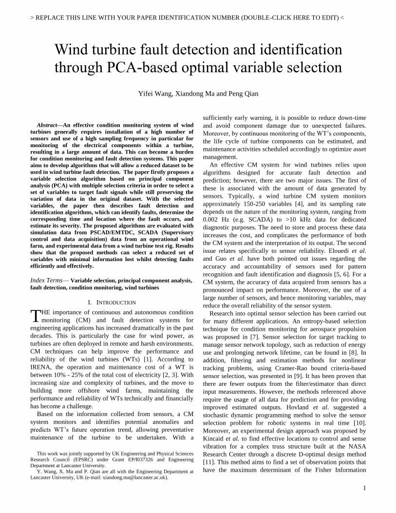
Fig. 1 shows the process of anomaly detection and
identification. During the training stage, a dataset from a
healthy turbine, that has a mean value of �̅�, is normalized to
zero mean and unit variance. Variables are selected via the
above T selection algorithm for a predefined fault signal. Then
the PCA model is created; its T2 statistic and threshold value
𝑇𝛼2 are calculated using (7) and (8) respectively. During the
testing stage, the data are normalized using the data from the
healthy turbine. The PCA model and the T2 statistics are also
calculated for the turbine data being evaluated. If any of the T2
statistics exceed the threshold value 𝑇𝛼2, as calculated from the
normal operational data, the measurement is considered to be
an anomaly. For the period where anomalies are present, the
T2 statistics are decomposed using (9) to determine which
variables have the highest contribution to the anomalies.
Normal operation data
Training stage
Data normalisation
PCA model
Calculation of T2 and threshold T2α
Testing data containing fault
Data normalisation
Calculation of T2 for testing data
T2>T2α
Testing stage
Anomaly detected
No anomaly
Calculation of TCi by decomposing T2
Loading (U) identification from PC
with the highest TCi
Anomaly detection phase
Anomaly identification phase
Fig. 1. Block diagram of the Hotelling’s T2 based fault detection and
identification algorithm.
C. Feature based fault severity estimation
In this section, an empirical model is proposed to detect a
specific fault, and then to estimate its severity under various
operation conditions. This is achieved using retained variables
from the T selection algorithm. Suppose there is a set of
variables X with dimension (n×q) obtained from the T
selection algorithm and related to a specific type of fault. To
build the detection model, measurement data for these
variables are collected multiple times 𝑿𝑑 at different fault
severities, where d indicates the index for each severity. PCA
is carried out for all these datasets, where d eigenvector
matrices U (q×q) and d eigenvalue vectors L (q×1) are
obtained. It can be shown that there is a relationship between
the fault severity Sv and eigenvalues L and eigenvectors U,
described as,
𝑆𝑣 = 𝑓(𝑢𝑖,𝑗, 𝐿𝑗), 1 < 𝑖 < 𝑞, 1 < 𝑗 < 𝑞 (10)

> REPLACE THIS LINE WITH YOUR PAPER IDENTIFICATION NUMBER (DOUBLE-CLICK HERE TO EDIT) <
4
The relationship function f is fault dependent, by which the
fault can be identified even at an incipient stage.
III. CASE STUDY - MONITORING DATA
A. Wind turbine simulation data
A 2 MW doubly-fed induction generator (DFIG) wind
turbine model with grid connection is simulated in
PSCAD/EMTDC. The simulation is based on the benchmark
model developed by PSCAD [24]. The model comprises a
mechanical model of a turbine, which simulates the blades’
aerodynamic behavior, a mechanical shaft, a generator, an
AC-DC-AC converter, and a grid network. This simulation is
primarily used for investigating the performance of wind
turbine’s transient and steady state conditions. The behavior of
the turbine during normal and faulty operations can also be
analyzed. Simulations are performed using wind speed data
collected at the Hazelrigg site near Lancaster University,
where a 2.1 MW wind turbine is installed and operating.
Measurements are taken from both internal and external nodes
of the simulated system under different operational conditions.
Computer simulations of a wind turbine incorporating a
permanent magnetic synchronous generator (PMSG) with a
grid connection have also been created. It is worth mentioning
that, in this paper, simulation data are used for severity
estimation of the faults in the turbine using the proposed
feature-based fault detection method.
B. SCADA data
SCADA data contains a large amount of information
regarding the operational and performance status of WTs.
Although SCADA data generally have low sampling rates,
they can provide an overview of a turbine’s operational and
performance status and condition, and have been employed
widely by researchers as the basis for CM systems. The
SCADA data used in this paper are taken from an operational
wind farm with 24 turbines in total. The condition of each
turbine is described by 128 variables, including temperatures,
vibrations, electrical parameters, wind speed, and digital
control signals. The data are sampled at an interval of one
second, but are averaged over 10 minutes and then stored on a
database for 15 months. Pre-processing of the data is
performed to eliminate digital signals, constant readings, and
error signals due to faulty sensors, which are ineffective to the
PCA analysis. Fault-free data are needed to train the model
with the proposed detection and identification algorithm. For
SCADA data, the active power versus wind speed curve, i.e.,
the S-curve, can be adopted to identify if the data are fault-
free, as concluded by S. Gill et al. [25]. The turbine that yields
an ideal S-curve after pre-processing is selected as the
reference healthy turbine.
C. Experimental wind turbine test rig
Experimental data from a WT test rig have also been collected
and used for further evaluation of the proposed algorithm. The
rig allows specific faults, such as phase-to-phase short circuit
faults, to be applied. The physical layout and overall
schematic of the test rig is shown in Fig. 2 and Fig.3,
respectively. The rotation of the turbine and the aerodynamics
of the blade are simulated by a computer and emulated with an
ABB 11 kW squirrel-cage induction motor controlled by a
frequency drive. The induction motor is directly coupled to a 3
kW PMSG generator from Mecc Alte. The use of this
induction motor incorporating the variable frequency drive can
ensure it provides the required torque to operate the generator
at different speeds. The AC-DC-AC converter consists of an
uncontrollable AC-DC rectifier, a DC-link capacitor and a
DC-AC inverter. The rectifier converts the mains voltage to a
DC voltage of 540V for DC-filtering and energy buffering via
the DC-Link capacitor. The IGBT inverter then converts the
DC power into an AC power at the desired output voltage and
frequency via the filter (Lf and Cf in Fig. 3). A DC-link
capacitor discharging circuit (R and Sd) is also added to
discharge the capacitor after the tests. The test rig operates in
an island mode, where all the generated power from the AC-
DC-AC converter is dissipated to an off-the-shelf resistive
load bank via a variable transformer. A number of transducers
and sensors are installed in the test rig to collect data for
control and monitoring purposes, including AC currents and
voltages before and after the converter, and the DC-link
current and voltage. All signals are interfaced to a data
acquisition card (NI USB-6229) through signal condition
modules for measurement data logging. The test rig is
controlled by a computer running LabVIEW, allowing real
time operation and measurements.
PC
Motor
Generator
Motor
drive
Load
Converter
DAQ
Sensors &
power
control
Fig. 2. Layout of the wind turbine test rig developed at Lancaster University
Peripheral components such as circuit breakers (CB) and
switches are also used in the test rig to assist the components
operation and for safety purposes. Due to safety issues, short
circuit faults are simulated under a controlled environment
where a resistance is added between phases to limit the
current. A switch is used to activate the fault for a given time
duration during operation of the test rig. Experiments are also
performed at a low-voltage level with constant wind speeds.

> REPLACE THIS LINE WITH YOUR PAPER IDENTIFICATION NUMBER (DOUBLE-CLICK HERE TO EDIT) <
5
IV. RESULTS AND ANALYSIS
A. Targeted variable selection
1) SCADA data
Considering initially the SCADA data, two types of fault
have been studied: a gearbox fault and a generator-related
fault. These faults were found by examining the SCADA data
together with the alarm log. A total of 77 variables were
obtained after pre-processing, consisting of electrical
variables, mechanical variables (angular speeds and
vibrations), and temperatures. Of these, 35 variables were
chosen to be the threshold for the selection algorithm, based
on SCREE plot analysis. The target variables, and the
respective performance measures for both fault-free data and
data from the faulty turbines are given in Table I.
TABLE I
PERFORMANCE MEASURES OF T SELECTION ALGORITHM WITH SCADA DATA
Type of data Original
data Gearbox fault Generator fault
Target signal
Gearbox
bearing
temperature
Generator
winding
temperature Cumulative variance,
cppv 100% 97.11% 97.42%
Average correlation, �̅� 0.3412 0.0677 0.0588
Percentage entropy, ηe 100% 75.91% 78.09%
It can be seen that both datasets have a cppv above 97%,
indicating the retained variables accommodate a high
percentage of the variance seen in the original dataset.
Moreover, there are significant reductions in the average
correlation for both datasets (0.0677 and 0.0588), compared to
the original data (0.3412). This implies a very low redundancy
amongst the retained variables. Finally, reasonable percentage
entropies are also obtained, with approximately 75.91% and
78.09% of the baseline value respectively.
In general, parameters such as wind speed, pitch angle,
environmental conditions (e.g. pressure, wind direction), and
vibrations are selected. It should be noted that the variables
selected by the T selection algorithm should share common
features with the targeting variable in the reduced dimensional
space; but this does not necessary mean the selected variables
must be physically close to it. For example, for a gearbox
fault, the gearbox bearing temperature is used as the targeting
variable; this does not mean that all variables relating to the
gearbox should be retained. In fact, if that was the case, the
retained variables could have very high redundancy.
2) ANN validation
This section addresses the problem in which the fault
feature is present in the retained variables. By adopting a
NARX (nonlinear autoregressive exogenous) ANN (Artificial
Neural Network) model, predictions between different input
variable sets can be compared. Three different input variable
sets are considered: the original dataset (without any
reduction), the first q PCs with a cumulative variance greater
than 0.95 [16], and the retained variables from the T selection
method.
The selection of input variables can greatly affect the
performance of the ANN model. With regards to fault
detection, it is preferable if the inputs are independent to the
output variable; thus, anomalies can be identified by
comparing the predicted and the actual outputs. If the input
variables share common features with the fault signal
(targeting variable), this could mean the model will match the
actual data, even during the period of a fault. Consequently,
the ANN model is used to further evaluate the retained
variables from the T selection algorithm, and to demonstrate
Resistive Load Bank
Vdc Cdc
g4
g3
g2
g1
g6
g5
Idc
VTorque Sensor
A
Lf Cf
A B C
IL, VL
Im, Vm
NI Data Acquisition CardIGBT Inverter
Controller
Signal Conditioning
Module
ABBMotorDrive
N
A
B
C
MainSupply
TInverter PWM
switching signals
Emulator Motor PMSG
Sm
CB
CB(Circuit
Breaker)
ω
AC/DC DC/AC
Filter
Transformer
PC with LabVIEW
Im, Vm: currents and voltages at machine sideIL, VL: currents and voltages at load sideIDC, VDC: current and voltage of the DC-link capacitorR: Discharging resistorSd: Discharging switchSm: Load switch
R
Sd
Fig. 3. Schematic block diagram of the wind turbine test rig

> REPLACE THIS LINE WITH YOUR PAPER IDENTIFICATION NUMBER (DOUBLE-CLICK HERE TO EDIT) <
6
whether the fault features of interest are still present in the
retained variables. A good model match is expected to be
obtained, especially during the period of the fault. The ANN
model established using the original dataset is used here as a
benchmark, with the squared correlation coefficient, R2, and
the root mean squared error (RMSE) are used to quantify the
model accuracy.
As an example, SCADA data with a gearbox-related fault
are used for evaluation. Fig. 4 shows the actual (red) and
predicted (blue) gearbox bearing temperature using different
input datasets. The anomaly occurs at approximately 720
hours, where the gearbox bearing temperature starts to
increase to an abnormal level. It can be seen that the
prediction using all of the data is very close to the actual
value, with RMSE and R2 of [0.276, 99.5%]. Similarly, in the
case of the targeted selection data, a high model prediction is
also obtained [0.397, 99.2%]. As for the PCA reduced data, it
has the worst performance of [1.793, 82.3%], where there is
an obvious difference between the actual and predicted
gearbox bearing temperature. It is worth mentioning that, for
all cases, the predictions during the fault-free period are very
similar. The difference between the actual and the predicted
value becomes clear when the fault begins. Based on these
results, it is straightforward to conclude that the dataset
retained by the T selection algorithm has captured the fault
signatures from the original dataset.
Fig. 4. Actual and predicted gearbox bearing temperatures from the ANN
model for three input SCADA datasets. Top: original dataset; middle: PCA reduced dataset; bottom: dataset obtained from T selection algorithm.
B. Hoteling’s T2 method
In this section, SCADA data are used to validate the
proposed Hoteling’s T2 detection and identification algorithm.
One of the assumptions made for T2 statistics is that the
original data should be approximately normally distributed.
Therefore, an additional pre-processing step is carried out to
normalize the data by means of a Box-cox transformation.
𝑥𝑖(𝜆) = {
𝑥𝑖𝜆 − 1
𝜆 if 𝜆 ≠ 0
ln(𝑥𝑖) if 𝜆 = 0
(11)
where x is the original data and λ is the coefficient optimized
through the maximum likelihood function such that the
resulting data is approximately normally distributed. The
distribution of wind speed before and after this transformation
is shown in Fig. 5.
Fig. 5. Example of histogram of wind speed from SCADA data before (top) and after (bottom) the Cox-box transformation
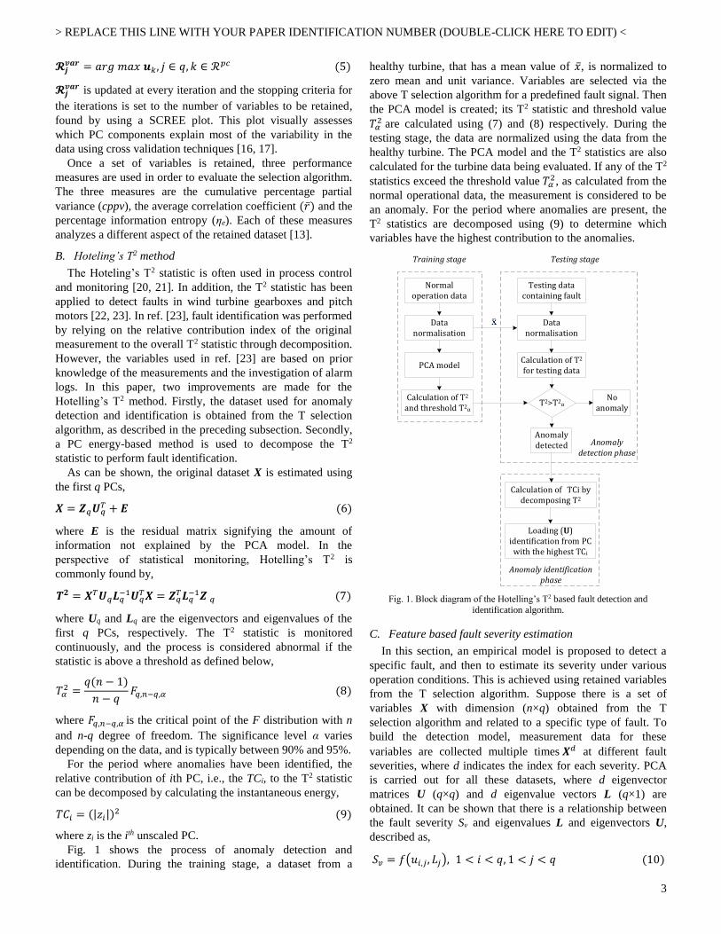
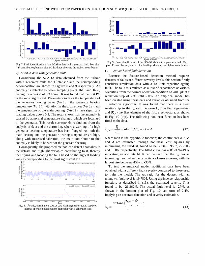
1) SCADA data with gearbox fault
The T2 statistic and the threshold of the normal operating
(top) and the test data with gearbox fault (bottom) are shown
in Fig. 6. As can be seen in the bottom plot, between sample
points 1400 to 1450 and 1510 to 1545, the T2 statistic is well
above the threshold. The SCADA data has a sampling rate of
10 minutes, which implies the detected anomalies lasted for a
period of 8 hours. By decomposing the T2 statistic, PC1 has
the highest contribution index (Fig. 7, top). The loading values
for PC1 are then shown in the bottom plot of Fig. 7. Any
loading, which is greater than the threshold value of 0.3, is
considered significant [17].
Fig. 7 shows that the active power (Var3), gearbox bearing
temperature (Var18) and gearbox oil sump temperature
(Var16) have the top three loading values. Other variables
with significant loadings are the generator bearing temperature
(Var15), power factor (Var5) and pitch motor 1 RPM (Var11).
This result indicates that the root cause of the fault might
occur at the cooling system of the gearbox; hence, the gearbox
bearing temperature is also increased. Furthermore, the turbine
data show a reduced active power output during the faulty
period, and a warning of a high gearbox temperature is also
found in the alarm log. The turbine was intentionally
controlled to operate at a lowered power rating in order to
avoid damaging the turbine. Evidently, the anomaly is related
to the gearbox.
Fig. 6. T2 statistic from the SCADA data with a gearbox fault. Top plot:
normal operation data; bottom plot: data with a gearbox fault
500 550 600 650 700 750 800 850
60
70
80
Bea
rin
g te
mp
all d
ata
500 550 600 650 700 750 800 850
60
70
80
Bea
rin
g te
mp
PC
A r
edu
ctio
n
500 550 600 650 700 750 800 850
60
70
80
Time (hours)
Bea
rin
g te
mp
targ
eted
sel
ecti
on
Actual value
Predicted value
Actual value
Predicted value
Actual value
Predicted value
-3 -2 -1 0 1 2 3 4 50
1000
2000
3000
Fre
qu
ency
Before transformation
-3 -2 -1 0 1 2 30
500
1000
1500
2000
Normalised wind speed
Fre
qu
ency
After transformation
Actual data
Fitted distribution
Actual data
Fitted distribution
0 0.2 0.4 0.6 0.8 1 1.2 1.4 1.6 1.8 2
x 104
10
20
30
40
50
T2
sta
tist
icn
orm
al o
per
atio
n d
ata
1100 1150 1200 1250 1300 1350 1400 1450 1500 15500
50
100
150
Time
T2
sta
tist
icfa
ult
y d
ata
Actual T2 statistic Threhold T2 statistic
> REPLACE THIS LINE WITH YOUR PAPER IDENTIFICATION NUMBER (DOUBLE-CLICK HERE TO EDIT) <
7
Fig. 7. Fault identification of the SCADA data with a gearbox fault. Top plot:
T2 contribution; bottom plot: PC loadings showing the highest contribution
2) SCADA data with generator fault
Considering the SCADA data obtained from the turbine
with a generator fault, the T2 statistic and the corresponding
decomposition are shown in Figures 8 and 9 respectively. An
anomaly is detected between sampling point 1610 and 1630,
lasting for a period of 3.3 hours. It was found that the first PC
is the most significant. Parameters such as the temperature of
the generator cooling water (Var13), the generator bearing
temperature (Var15), vibration in the z direction (Var12), and
the temperature of the main bearing (Var11) have significant
loading values above 0.3. The result shows that the anomaly is
caused by abnormal temperature changes, which are localized
in the generator. This result corresponds to findings from the
analysis of data and the alarm log, where a warning of a high
generator bearing temperature has been flagged. As both the
main bearing and the generator bearing temperature are high,
along with increased vibration, the main contributor to this
anomaly is likely to be wear of the generator bearing.
Consequently, the proposed method can detect anomalies in
the dataset and highlight variables contributing to it, thereby
identifying and locating the fault based on the highest loading
values corresponding to the most significant PC.
Fig. 8. T2 statistic from the SCADA data with a generator fault. Top plot:
normal operation data; bottom plot: data with a generator fault
Fig. 9. Fault identification of the SCADA data with a generator fault. Top
plot: T2 contribution; bottom plot: loadings showing the highest contribution
C. Feature based fault detection
Because the feature-based detection method requires
datasets of faults at different severity levels, this section firstly
considers simulation data with a DC-link capacitor ageing
fault. The fault is simulated as a loss of capacitance at various
severities, from the normal operation condition of 7800 μF at a
reduction step of -5% until -50%. An empirical model has
been created using these data and variables obtained from the
T selection algorithm. It was found that there is a clear
relationship to the rl/u ratio between 𝐋1𝑟 (the first eigenvalue)
and 𝐔1,1𝑟 (the first element of the first eigenvector), as shown
in Fig. 10 (top). The following nonlinear function has been
fitted to the data,
𝑟𝑙/𝑢 =𝑙1𝑟
𝑢1,1𝑟 = 𝑎tanh(𝑏𝑆𝑣 + 𝑐) + 𝑑 (12)
where tanh is the hyperbolic function; the coefficients a, b, c,
and d are estimated through nonlinear least squares by
minimizing the residual, found to be 3.234, 0.9597, -5.7903
and 19.06, respectively. The fitted curve has a R2 of 94.49%,
indicating an accurate fit. It can be seen that the rl/u has an
increasing trend when the capacitance losses increase, with the
largest rise between -15% to -35%.
To test the empirical model, additional data have been
obtained with a different fault severity compared to those used
to train the model. The rl/u ratio for the dataset with an
unknown fault level is 19.7805. Using the inverse relationship
function, as described in (13), the estimated severity Sv is
found to be -26.362%. The actual fault level is -27%, as
shown in the bottom plot of Fig. 10, an error of 2.4%,
implying an accurate detection and severity estimation.
𝑆𝑣 =arctanh (
𝑟𝑙/𝑢 − 𝑑𝑎
) − c
𝑏 (13)
PC1 PC2 PC3 PC4 PC5 PC6 PC7 PC8 PC9 PC10 PC11 PC12 PC13 PC14 PC15 PC16 PC17 PC180
500
1000
1500T
2 c
on
trib
uti
on
Principal components
Var1 Var2 Var3 Var4 Var5 Var6 Var7 Var8 Var9 Var10Var11Var12Var13Var14Var15Var16Var17Var18-0.4
-0.2
0
0.2
0.4
Original variables
Lo
adin
g o
f P
C 1
0 0.2 0.4 0.6 0.8 1 1.2 1.4 1.6 1.8 2
x 104
10
20
30
40
50
60
T2
sta
tist
icn
orm
al o
per
atio
n d
ata
1500 1520 1540 1560 1580 1600 1620 1640 1660 1680 1700
0
20
40
60
80
Time
T2
sta
tist
icfa
ult
y d
ata
Actual T2 statistic Threhold T2 statistic
Actual T2 statistic Threhold T2 statistic
PC1 PC2 PC3 PC4 PC5 PC6 PC7 PC8 PC9 PC10 PC11 PC12 PC13 PC14 PC15 PC16 PC17 PC180
100
200
300
400
Principal components
T2 c
on
trib
uti
on
Var1 Var2 Var3 Var4 Var5 Var6 Var7 Var8 Var9 Var10Var11Var12Var13Var14Var15Var16Var17Var18-0.4
-0.2
0
0.2
0.4
Original variables
Lo
adin
g o
f P
C 1
> REPLACE THIS LINE WITH YOUR PAPER IDENTIFICATION NUMBER (DOUBLE-CLICK HERE TO EDIT) <
8
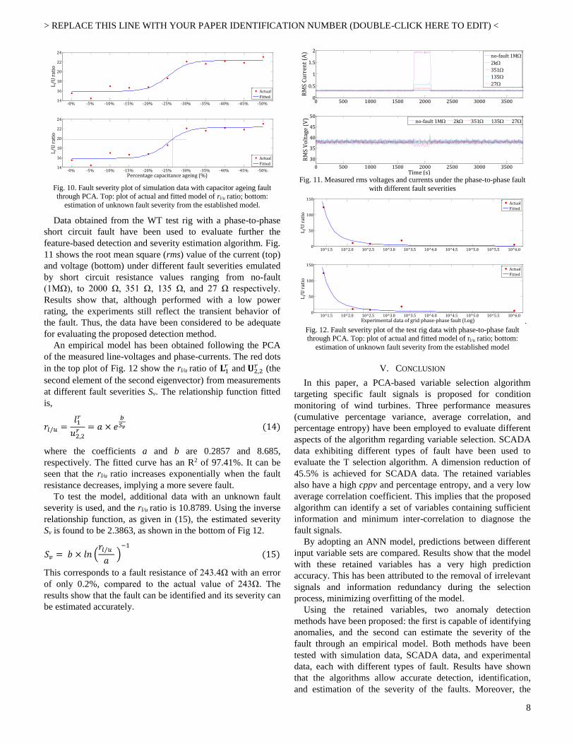
Fig. 10. Fault severity plot of simulation data with capacitor ageing fault through PCA. Top: plot of actual and fitted model of rl/u ratio; bottom:
estimation of unknown fault severity from the established model.
Data obtained from the WT test rig with a phase-to-phase
short circuit fault have been used to evaluate further the
feature-based detection and severity estimation algorithm. Fig.
11 shows the root mean square (rms) value of the current (top)
and voltage (bottom) under different fault severities emulated
by short circuit resistance values ranging from no-fault
(1MΩ), to 2000 Ω, 351 Ω, 135 Ω, and 27 Ω respectively.
Results show that, although performed with a low power
rating, the experiments still reflect the transient behavior of
the fault. Thus, the data have been considered to be adequate
for evaluating the proposed detection method.
An empirical model has been obtained following the PCA
of the measured line-voltages and phase-currents. The red dots
in the top plot of Fig. 12 show the rl/u ratio of 𝐋1𝑟 and 𝐔2,2
𝑟 (the
second element of the second eigenvector) from measurements
at different fault severities Sv. The relationship function fitted
is,
𝑟𝑙/𝑢 =𝑙1𝑟
𝑢2,2𝑟 = 𝑎 × 𝑒
𝑏𝑆𝑣 (14)
where the coefficients a and b are 0.2857 and 8.685,
respectively. The fitted curve has an R2 of 97.41%. It can be
seen that the rl/u ratio increases exponentially when the fault
resistance decreases, implying a more severe fault.
To test the model, additional data with an unknown fault
severity is used, and the rl/u ratio is 10.8789. Using the inverse
relationship function, as given in (15), the estimated severity
Sv is found to be 2.3863, as shown in the bottom of Fig 12.
𝑆𝑣 = 𝑏 × 𝑙𝑛 (𝑟𝑙/𝑢
𝑎 )−1
(15)
This corresponds to a fault resistance of 243.4Ω with an error
of only 0.2%, compared to the actual value of 243Ω. The
results show that the fault can be identified and its severity can
be estimated accurately.
Fig. 11. Measured rms voltages and currents under the phase-to-phase fault
with different fault severities
.
Fig. 12. Fault severity plot of the test rig data with phase-to-phase fault through PCA. Top: plot of actual and fitted model of rl/u ratio; bottom:
estimation of unknown fault severity from the established model
V. CONCLUSION
In this paper, a PCA-based variable selection algorithm
targeting specific fault signals is proposed for condition
monitoring of wind turbines. Three performance measures
(cumulative percentage variance, average correlation, and
percentage entropy) have been employed to evaluate different
aspects of the algorithm regarding variable selection. SCADA
data exhibiting different types of fault have been used to
evaluate the T selection algorithm. A dimension reduction of
45.5% is achieved for SCADA data. The retained variables
also have a high cppv and percentage entropy, and a very low
average correlation coefficient. This implies that the proposed
algorithm can identify a set of variables containing sufficient
information and minimum inter-correlation to diagnose the
fault signals.
By adopting an ANN model, predictions between different
input variable sets are compared. Results show that the model
with these retained variables has a very high prediction
accuracy. This has been attributed to the removal of irrelevant
signals and information redundancy during the selection
process, minimizing overfitting of the model.
Using the retained variables, two anomaly detection
methods have been proposed: the first is capable of identifying
anomalies, and the second can estimate the severity of the
fault through an empirical model. Both methods have been
tested with simulation data, SCADA data, and experimental
data, each with different types of fault. Results have shown
that the algorithms allow accurate detection, identification,
and estimation of the severity of the faults. Moreover, the
-0% -5% -10% -15% -20% -25% -30% -35% -40% -45% -50%14
16
18
20
22
24L
/U r
atio
-0% -5% -10% -15% -20% -25% -30% -35% -40% -45% -50%14
16
18
20
22
24
Percentage capacitance ageing (%)
L/U
rat
io
Actual
Fitted
Actual
Fitted
0 500 1000 1500 2000 2500 3000 35000
0.5
1
1.5
2
RM
S C
urr
ent
(A)
0 500 1000 1500 2000 2500 3000 3500
30
35
40
45
50
RM
S V
olt
age
(V)
Time (s)
no-fault 1M
2k
351
135
27
no-fault 1M 2k 351 135 27
10^1.5 10^2.0 10^2.5 10^3.0 10^3.5 10^4.0 10^4.5 10^5.0 10^5.5 10^6.00
50
100
150
L/U
rat
io
10^1.5 10^2.0 10^2.5 10^3.0 10^3.5 10^4.0 10^4.5 10^5.0 10^5.5 10^6.00
50
100
150
Experimental data of grid phase-phase fault (Log)
L/U
rat
io
Actual
Fitted
Actual
Fitted

> REPLACE THIS LINE WITH YOUR PAPER IDENTIFICATION NUMBER (DOUBLE-CLICK HERE TO EDIT) <
9
proposed methods require minimal human interaction once the
model is built. Consequently, the method possesses great
potential in developing an autonomous condition monitoring
system. In future studies, the development of the algorithms in
real-time for online monitoring purposes will be investigated,
and selection methods based on nonlinear algorithms will be
analyzed.
ACKNOWLEDGMENT
The permission of use SCADA data from Wind Prospect
Ltd are gratefully acknowledged.
REFERENCES
[1] F. Spinato, P.J. Tavner, G.J.W. van Bussel, E. Koutoulakos, “Reliability
of wind turbine subassemblies,” IET Renewable Power Generation, 2009, Vol. 3, Issue 4, pp. 287-401.
[2] IRENA, “Renewable energy technologies: cost analysis series,” Jun
2012.
[3] Y. Lin, L. Tu, H. Liu, W. Li, “Fault analysis of wind turbines in China,”
Renewable and Sustainable Energy Reviews, Vol. 553, pp. 482-490, 2016.
[4] X. Ma, “Novel early waning fault detection for wind turbine-based DG
systems,” Proceedings of 2nd IEEE PES International Conference and Exhibition on Innovative Smart Grid Technologies (ISGT Europe), 2011,
Manchester, UK.
[5] Z. Elouedi, K. Mellouli, P. Smets, “Assessing sensor reliability for multisensor data fusion within the transferable belief model,” IEEE
Transactions on Systems, Man and Cybernetics – Part B: Cybernetics,
Vol. 34, pp. 782 - 787, 2004. [6] H. Guo, W. Shi, Y. Deng, “Evaluating sensor reliability in classification
problems based on evidence theory,” IEEE Transactions on Systems,
Man and Cybernetics – Part B: Cybernetics, Vol. 36, pp. 970 - 981, 2006.
[7] L. Liu, S. Wang, D. Liu, Y. Zhang and Y. Peng, “Entropy-based sensor
selection for condition monitoring and prognostics of aircraft engine,” Microelectronics Reliability, Vol. 55, pp. 2092-2096, 2015.
[8] X. Shen, S. Liu, and P. Varshney, “Sensor selection for nonlinear
systems in large sensor networks,” IEEE Transaction on Aerospace and Electronics Systems, Vol 50, pp. 2664-2678, 2014.
[9] A. Mohammadi, A. Asif, “Consensus-based distributed dynamic sensor
selection in decentralised sensor networks using the posterior Cramer-Rao lower bound,” Signal Processing, Vol. 108, pp. 558-575, 2015
[10] G. Hovland and B. McCarragher, “Control of sensory perception in
discrete event systems using stochastic dynamic programming,” Journal of Dynamic Systems, Measurement and Control, Vol. 121, pp. 200-205,
1999.
[11] K. Kincaid and S. Padula, “D-optimal designs for sensor and actuator locations,” Compute. Oper. Res., Vol. 29, no. 6, pp. 701–713, 2002.
[12] W. Zhang, X. Ma, “Simultaneous fault detection and sensor selection for
condition monitoring of wind turbines,” Energies, Vol.9, no.4, pp. 280, 2016.
[13] Y. Wang, X. Ma and M. J. Joyce, “Reducing sensor complexity for
monitoring wind turbine performance using principal component analysis,” Renewable energy, Vol. 97, pp. 444-456, 2016.
[14] M.D. Farrell, M.M. Russell, “On the impact of PCA dimension
reduction for hyperspectral detection of difficult targets,” IEEE Geoscience and Remote Sensing Letters, Vol., 2, no.2, 2005.
[15] A. Malhi, R.X. Gao, “PCA-based feature selection scheme for machine
defect classification,” IEEE Transactions on Instrumentation and Measurement, Vol. 53, no.6, 2004.
[16] J. Jackson, “Users guide to principal components,” A Wiley -
Interscience Publication, ISBN 0-471-62267-2,1991 [17] I.T. Jolliffe, “Principal component analysis,” New York: Springer. 2002.
ISBN: 978-0387954424.
[18] E.M.L. Beale, M.G. Kendall and D.W. Mann, “The discarding of variables in multivariate analysis,” Biometrika, Vol. 54, pp. 357-366,
1967.
[19] J.A. Cumming, D.A. Wooff, “Dimension reduction via principal variables,” Computational statistics & data analysis, Vol. 52, pp. 550-
565, 2007.
[20] J. MacGregor, and T. Kourti, “Statistical process control of multivariate
processes” Control Engineering Practice, Vol.3, no.3, pp.403-414, 1995.
[21] D.C. Montgomery, “Introduction to statistical quality control,” 7th ed.,
Wiley: New York, 2013, NY, USA. [22] K. Kim, S. Sheng, and P. Fleming, “Use of SCADA data for failure
detection in wind turbines,” Energy Sustainability Conference and Fuel
Cell Conference, August 7-10, 2011, Washington, D.C. [23] H. Yang, M. Huang, and S. Yang, “Integrating auto-associative neural
networks with Hotelling T2 control charts for wind turbine fault
detection,” Energies, Vol. 8, pp. 12100-12115, 2015. [24] Wind turbine application technical paper, PSCAD version 4.2, Power
system simulation, CEDRAT, 2006.
[25] S. Gill, B. Stephen, S. Galloway, “Wind turbine condition assessment through power curve copula modeling,” IEEE Transaction on
Sustainable Energy, Vol. 3, no. 1, 2012.
Yifei Wang received a BEng degree in
mechanical engineer from University of
Malta in 2010, and MSc and PhD degree
from Lancaster University in 2011 and
2016, respectively. His research interest
includes data mining, hardware and
software design for condition monitoring
and fault diagnosis of the wind power
generation system.
Xiandong Ma received a BEng degree in
electrical engineering in 1986, an MSc
degree in power systems and automation
in 1989 and a PhD in partial discharge-
based high-voltage condition monitoring
in 2003. He is currently a Senior Lecturer
in the Engineering Department at
Lancaster University, UK. His research
interests include intelligent condition
monitoring and fault diagnosis of distributed generation
systems with wind turbines with an emphasis on analytical and
experimental investigation, advanced signal processing, data
mining and instrumentation, and electromagnetic NDT testing
and imaging.
Peng Qian received a BEng degree in
electrical engineering and automation in
2009 and an MSc degree in power
electronics and drives in 2014, both from
Jiangsu University, China. He has been
pursuing his PhD studies in condition
monitoring of wind turbines at Lancaster
University, UK, since January 2015. His
research interests include predictive condition monitoring,
data driven-based modelling, optimal energy management and
hardware-in-the-loop testing.


