
When Two Choices Are not Enough: Balancing at Scale in Distributed Stream Processing
Muhammad Anis Uddin Nasir, Gianmarco De Francisci Morales, Nicolas Kourtellis, Marco Serafini
International Conference on Data Engineering (ICDE 2016)

Stream Processing
• Streaming Application
– Online Machine Learning
– Real Time Query Processing
– Continuous Computation
• Streaming Frameworks
– Storm, S4, Flink Streaming, Spark Streaming
2

Stream Processing Model
• Streaming Applications are represented by Directed Acyclic Graphs (DAGs)
Data Stream
Operators
Data Channels
Worker
Worker
Worker
Source
Source
3

Challenges
4
Velocity
Volume
Skewness

Problem Formulation
• Input is a unbounded sequence of messages from a key distribution
• Each message is assigned to a worker for processing (i.e., filter, aggregate, join)
• Load balance properties– Processing Load Balance
• Metric: Load Imbalance
5

Stream Grouping
1. Key or Fields Grouping (Hash-Based)– Single worker per key– Stateful operators
2. Shuffle Grouping (Round Robin)– All workers per key– Stateless Operators
3. Partial Key Grouping– Two workers per key– MapReduce-like Operators
6

Key Grouping
• Key Grouping• Scalable✖• Low Memory ✔• Load Imbalance ✖
Worker
Worker
Worker
Source
Source
7
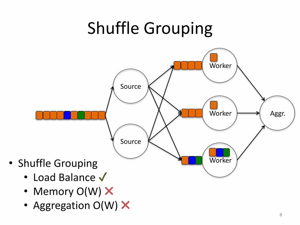
Shuffle Grouping
• Shuffle Grouping• Load Balance ✔• Memory O(W) ✖• Aggregation O(W) ✖
8
Worker
Worker
Worker
Aggr.
Source
Source

Partial Key Grouping
• Partial Key Grouping• Scalable✖• Low Memory ✔• Load Imbalance ✖
9
Worker
Worker
Worker
Aggr.
Source
Source

Partial Key Grouping
10
P1 = 9.32%
10-7
10-6
10-5
10-4
10-3
10-2
10-1
5 10 20 50 100
WP
Imb
ala
nce
I(m
)
Workers
PKGD-CW-C
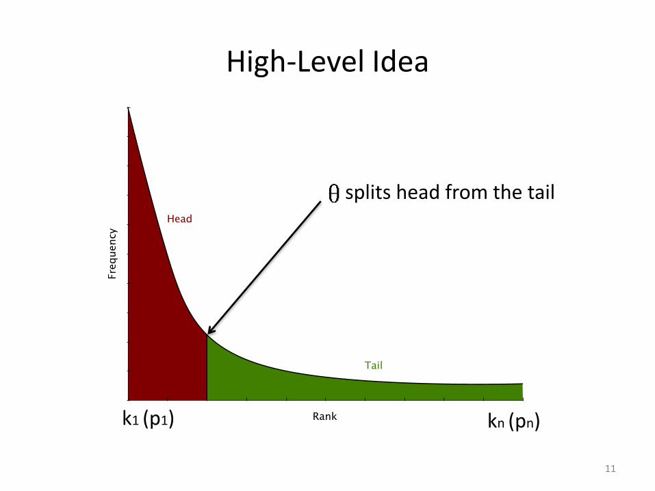
High-Level Idea
11
splits head from the tail
k1 (p1) kn (pn)

How to find the optimal threshold?
• Any key that exceeds the capacity of two workers requires more than two workers pi ≥ 2/(n)
• We need to consider the collision of the keys while deciding the number of workers
• PKG guarantees nearly perfect load balance for p1 ≤ 1/(5n)
12

How to find optimal threshold?
13
10-7
10-6
10-5
10-4
10-3
10-2
10-1
100
0.4 0.8 1.2 1.6 2
W-C
Imba
lan
ce I(m
)n=50
2/n1/n
1/2n1/4n1/8n
10-7
10-6
10-5
10-4
10-3
10-2
10-1
100
0.4 0.8 1.2 1.6 2
W-C
n=100
10-7
10-6
10-5
10-4
10-3
10-2
10-1
100
0.4 0.8 1.2 1.6 2
RR
Imba
lance I
(m)
Skew
10-7
10-6
10-5
10-4
10-3
10-2
10-1
100
0.4 0.8 1.2 1.6 2
RR
Skew

How many keys are in the head?
• Plots for the number of keys in head for two different thresholds
14

How many workers for the head?
• D-Choices: – adapts to the frequencies of the keys in the head
– requires load imbalance as an input parameter
– memory efficient
• W-Choices: – allows all the workers for the keys in the head
– does not require any input parameters
– requires more compared to D-Choices
15
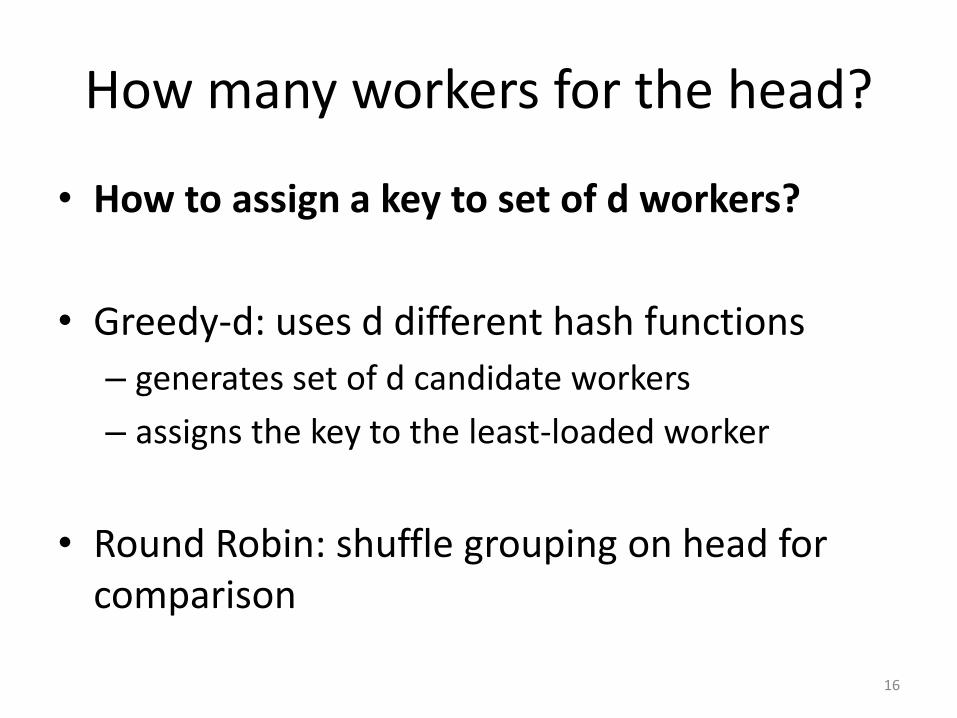
How many workers for the head?
• How to assign a key to set of d workers?
• Greedy-d: uses d different hash functions
– generates set of d candidate workers
– assigns the key to the least-loaded worker
• Round Robin: shuffle grouping on head for comparison
16

How to find the optimal d?
17
• Optimization problem:

• We rewrite the constraint:
• For instance for the first key with p1:
How to find the optimal d?
18
pii£h
å +b
n
æ
èç
ö
ø÷
d
pih<i£H
å +b
n
æ
èç
ö
ø÷
2
pii>H
å £b
n
æ
èç
ö
ø÷+e
p1 +b
n
æ
èç
ö
ø÷
d
pi1<i£H
å +b
n
æ
èç
ö
ø÷
2
pii>H
å £b
n
æ
èç
ö
ø÷+e

• We rewrite the constraint:
where
How to find the optimal d?
19
pii£h
å +b
n
æ
èç
ö
ø÷
d
pih<i£H
å +b
n
æ
èç
ö
ø÷
2
pii>H
å £b
n
æ
èç
ö
ø÷+e
b = n-nn-1
n
æ
èç
ö
ø÷
h´d

What are the values of d?
20
0
0.2
0.4
0.6
0.8
1
0.4 0.8 1.2 1.6 2
Fra
ctio
n o
f w
ork
ers
(d/n
)
Skew
n=5n=10n=50
n=100

Memory Overhead
21
0
10
20
30
0.4 0.8 1.2 1.6 2Me
mo
ry w
.r.t
PK
G (
%)
Skew
n=50
D-CW-C
0.4 0.8 1.2 1.6 2
Skew
n=100
• Compared to PKG

Memory Overhead
22
• Compared to SG
-100
-90
-80
-70
0.4 0.8 1.2 1.6 2
Me
mory
w.r
.t S
G (
%)
Skew
n=50
D-CW-C
0.4 0.8 1.2 1.6 2
Skew
n=100
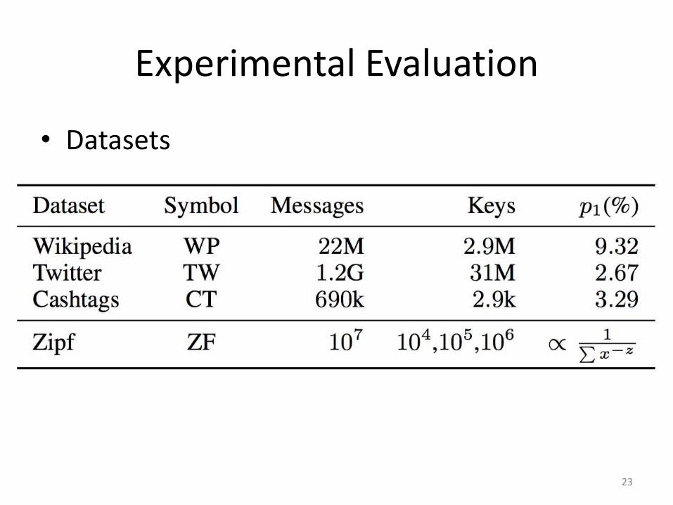
Experimental Evaluation
• Datasets
23

Experimental Evaluation
• Algorithms
24

How good are estimated d?
• Estimated d vs. the minimal experimental value of d
25
0
0.2
0.4
0.6
0.8
1
0.4 0.8 1.2 1.6 2
Fra
ctio
n o
f w
ork
ers
(d
/n)
Skew
n=50
Minimal-dD-C
0.4 0.8 1.2 1.6 2
Skew
n=100

Load Imbalance for Zipf
26

Load balance for real workloads
• Comparison of D-C, WC with PKG
27

Load Imbalance over time
• Load imbalance over time for the real-world datasets
28
10-9
10-8
10-7
10-6
10-5
0 5 10 15 20 25
WPWP
Imba
lan
ce I(t
)
n=20
10-9
10-8
10-7
10-6
0 5 10 15 20 25
n=50
10-8
10-7
10-6
10-5
10-4
10-3
10-2
0 5 10 15 20 25
n=100
PKGD-CW-C
10-7
10-6
10-5
10-4
10-3
10-2
0 5 10 15 20 25 30 35
TW
Imb
ala
nce I(t
)
10-7
10-6
10-5
10-4
10-3
10-2
10-1
0 5 10 15 20 25 30 3510
-8
10-7
10-6
10-5
10-4
10-3
10-2
10-1
0 5 10 15 20 25 30 35

Throughput on real DSPE
29
• Throughput on a cluster deployment on Apache Storm for KG, PKG, SG, D-C, and W-C on the ZF dataset
0
500
1000
1500
2000
2500
3000
3500
KG PKG D-C W-C SG
Th
rou
ghp
ut (e
ve
nts
/seco
nd
)
z=1.4z=1.7z=2.0

Latency on a real DSPE
30
• Latency (on a cluster deployment on Apache Storm) for KG, PKG, SG, D-C, and W-C
0
500
1000
1500
2000
2500
3000
3500
4000
4500
KG PKG D-C W-C SG
La
ten
cy (
ms)
z=1.4
max avgp50p95p99
KG PKG D-C W-C SG
z=1.7
KG PKG D-C W-C SG
z=2.0

Conclusion
• We propose two algorithms to achieve loadbalance at scale for DSPEs
• Use heavy hitters to separate the head of the distribution and process on larger set of workers
• Improvement translates into 150% gain in throughput and 60% gain in latency over PKG
31

When Two Choices Are not Enough: Balancing at Scale in Distributed Stream Processing
Muhammad Anis Uddin Nasir, Gianmarco De Francisci Morales, Nicolas Kourtellis, Marco Serafini
International Conference on Data Engineering (ICDE 2016)


