When Fast Growing Economies Slow Down:
International Evidence and Implications for China
Barry Eichengreen, Donghyun Park and
Kwanho Shin March 2011
1

Motivation
• Rapid growth of emerging markets is one of the premier facts of the 21st century.
• We take their rapid growth for granted.
• A sharp slowdown would have major implications for: – Global growth
– Global imbalances
– Political and social stability • Among other things…
2

Motivation
• So is a significant slowdown in growth in emerging markets coming?
• Historical evidence strongly suggests so: all fast-growing economies have slowed down at some point.
• Growth theory suggests this: that growth slows down as a catch-up economy begins to approach the technological frontier.
• The questions is: at what point, precisely, does the slowdown occur?
3

Motivation
• In this paper we address the issue in general and its implications for China in particular.
• Why the Chinese case is particularly pertinent: – China is a large fraction of the world economy.
– China accounts for an important fraction of incremental global demand.
– Its demand matters for exporters of capital goods.
– Its demand matters for prices of energy, foodstuffs and other commodities.
– Its demand matters for East Asia in particular.
4

Growth Slowdown - Definition
• Our analysis of growth slowdowns builds on a symmetrical analysis of growth accelerations by Hausmann, Pritchett and Rodrik (2005). We identify an episode as a growth slowdown if the rate of GDP growth satisfies three conditions: – Growth is at least 3.5 per cent over the initial 7 year
period. – Income per capita is at least $10,000 US (2007 PPP
prices). – The growth slowdown between successive 7 year
periods is at least 2 percentage points.
5

Sensitivity
• Note that our PWT data end in 2007, which accounts for the absence of potential recent slowdowns some people may have in mind.
• Note that we do extensive sensitivity analysis. – Alter the 7 year window.
– Lower the $10,000 per capita income threshold designed to exclude chronic slow-growth poor economies.
– Treat oil exporters separately.
6

Growth Slowdown Episodes
• Table 1 lists all the slowdowns identified by this approach. • In some cases the methodology identifies a string of
consecutive years as growth slowdowns. – For Greece, for example, all years between 1969 and 1978 are
identified as a slowdown.
• One way of dealing with this is to employ a Chow test for structural breaks to select only one year out of the consecutive years identified. – For Greece we would then select 1973 as the year of growth
slowdown because the Chow test is most significant for that year.
• In Table 1, the years chosen by the Chow test are denoted in bold face.
7
Construction of Dummy
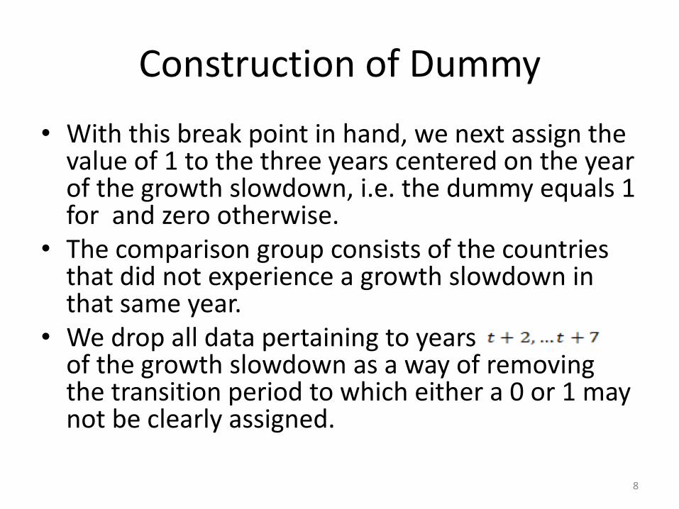
• With this break point in hand, we next assign the value of 1 to the three years centered on the year of the growth slowdown, i.e. the dummy equals 1 for and zero otherwise.
• The comparison group consists of the countries that did not experience a growth slowdown in that same year.
• We drop all data pertaining to years of the growth slowdown as a way of removing the transition period to which either a 0 or 1 may not be clearly assigned.
8
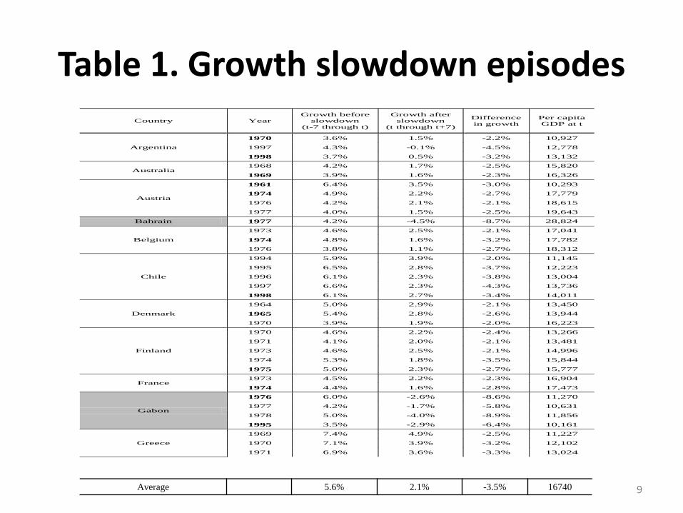
Table 1. Growth slowdown episodes
9
Country Year
Growth before
slowdown
(t-7 through t)
Growth after
slowdown
(t through t+7)
Difference
in growth
Per capita
GDP at t
Argentina
1970 3.6% 1.5% -2.2% 10,927
1997 4.3% -0.1% -4.5% 12,778
1998 3.7% 0.5% -3.2% 13,132
Australia 1968 4.2% 1.7% -2.5% 15,820
1969 3.9% 1.6% -2.3% 16,326
Austria
1961 6.4% 3.5% -3.0% 10,293
1974 4.9% 2.2% -2.7% 17,779
1976 4.2% 2.1% -2.1% 18,615
1977 4.0% 1.5% -2.5% 19,643
Bahrain 1977 4.2% -4.5% -8.7% 28,824
Belgium
1973 4.6% 2.5% -2.1% 17,041
1974 4.8% 1.6% -3.2% 17,782
1976 3.8% 1.1% -2.7% 18,312
Chile
1994 5.9% 3.9% -2.0% 11,145
1995 6.5% 2.8% -3.7% 12,223
1996 6.1% 2.3% -3.8% 13,004
1997 6.6% 2.3% -4.3% 13,736
1998 6.1% 2.7% -3.4% 14,011
Denmark
1964 5.0% 2.9% -2.1% 13,450
1965 5.4% 2.8% -2.6% 13,944
1970 3.9% 1.9% -2.0% 16,223
Finland
1970 4.6% 2.2% -2.4% 13,266
1971 4.1% 2.0% -2.1% 13,481
1973 4.6% 2.5% -2.1% 14,996
1974 5.3% 1.8% -3.5% 15,844
1975 5.0% 2.3% -2.7% 15,777
France 1973 4.5% 2.2% -2.3% 16,904
1974 4.4% 1.6% -2.8% 17,473
Gabon
1976 6.0% -2.6% -8.6% 11,270
1977 4.2% -1.7% -5.8% 10,631
1978 5.0% -4.0% -8.9% 11,856
1995 3.5% -2.9% -6.4% 10,161
Greece
1969 7.4% 4.9% -2.5% 11,227
1970 7.1% 3.9% -3.2% 12,102
1971 6.9% 3.6% -3.3% 13,024
Average 5.6% 2.1% -3.5% 16740
Simple Average Statistics
• At the bottom of Table 1 we report the average values for all non-oil-exporting countries. On average, high growth came to an end at a per capita GDP of $16,740, in 2005 constant international prices. – The median is $15,058.
• At that point the growth rate slowed from 5.6 to 2.1 per cent per annum. – For purposes of comparison, note that China’s per capita
GDP, in constant 2005 international prices, was $8,511 as of 2007, India’s $3.826, Brazil’s $9,645. These are the latest compatible figures provided by Penn World Tables.
10
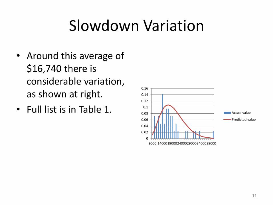
Slowdown Variation
• Around this average of $16,740 there is considerable variation, as shown at right.
• Full list is in Table 1.
0
0.02
0.04
0.06
0.08
0.1
0.12
0.14
0.16
9000 140001900024000290003400039000
Actual value
Predicted value
11

Some comments on Table 1 list
• Passes the smell test: many of the cases are well known.
• Second, in the majority of the countries experiencing slowdowns, this event is centered at a single point in time and a particular level of per capita income.
• Oil exporters also are unusual in that they are able to maintain high rates until higher per capita incomes are reached than is customary for other countries.
12

Growth accounting results
• Question: what grows more slowly around times of slowdowns: capital, labor or productivity?
• Answer (in Table 2): 85 per cent of the slowdown in the rate of growth of output is explained by the slowdown in the rate of TFP growth.
• Evidently, slowdowns coincide with the point in the growth process where it is no longer possible to boost productivity by shifting additional workers from agriculture to industry and where the gains from importing foreign technology diminish.
13

Table 2. Growth accounting results
14
Country Year
Capital Labor Human Capital Labor
Before
Slowdown
After
Slowdown
Before
Slowdown
After
Slowdown
Before
Slowdown
After
Slowdown
Before
Slowdown
After
Slowdown
Australia 1968 1.66% 1.41% 1.45% 1.46% 0.34% 0.60% 2.62% 0.05%
1969 1.71% 1.29% 1.51% 1.35% 0.39% 0.62% 2.23% -0.02%
Austria
1961 1.92% 1.95% -0.06% 0.23% 1.12% 1.10%
1974 1.97% 1.35% 0.15% 0.47% 0.68% 0.38% 2.55% -0.01%
1976 1.85% 1.14% 0.24% 0.64% 0.55% 0.35% 1.84% 0.00%
1977 1.79% 0.99% 0.30% 0.67% 0.47% 0.35% 1.63% -0.55%
Belgium
1973 1.20% 0.98% 0.24% 0.45% 0.38% 0.55% 3.17% 0.71%
1974 1.21% 0.85% 0.27% 0.46% 0.44% 0.53% 3.21% -0.12%
1976 1.13% 0.65% 0.37% 0.47% 0.54% 0.51% 2.06% -0.47%
Chile
1994 1.93% 2.89% 0.98% 0.98% 0.47% 0.31% 4.22% 1.05%
1995 2.35% 2.61% 0.94% 1.00% 0.42% 0.32% 4.39% 0.08%
1996 2.63% 2.38% 0.92% 1.01% 0.37% 0.33% 3.78% -0.25%
1997 2.90% 2.18% 0.91% 1.02% 0.33% 0.34% 4.01% -0.08%
1998 3.13% 2.12% 0.91% 1.01% 0.32% 0.36% 3.18% 0.37%
Denmark
1964 1.50% 1.69% 0.43% 0.22% 0.32% 1.17%
1965 1.70% 1.62% 0.38% 0.23% 0.34% 1.13%
1970 1.76% 1.24% 0.48% 0.28% 0.30% 0.38% 2.10% 0.46%
Finland
1970 1.60% 1.47% 0.54% 0.49% 0.63% 0.83% 2.10% -0.20%
1971 1.63% 1.29% 0.44% 0.47% 0.67% 0.81% 1.59% -0.14%
1973 1.56% 1.14% 0.43% 0.35% 0.73% 0.77% 2.13% 0.56%
1974 1.64% 0.99% 0.42% 0.33% 0.76% 0.65% 2.71% 0.17%
1975 1.70% 0.88% 0.42% 0.33% 0.79% 0.53% 2.41% 0.90%
France 1973 1.74% 1.09% 0.63% 0.56% 0.54% 0.51% 2.45% 0.49%
1974 1.72% 0.95% 0.63% 0.61% 0.55% 0.50% 2.37% 0.02%
Greece
1969 2.14% 1.86% 0.22% 0.43% -0.43% 0.22% 6.01% 2.98%
1970 2.15% 1.68% 0.12% 0.62% -0.31% 0.27% 5.64% 2.12%
1971 2.10% 1.49% 0.09% 0.75% -0.14% 0.28% 5.38% 2.04%
1972 2.07% 1.25% 0.11% 0.83% 0.04% 0.28% 5.32% 1.10%
1973 2.14% 0.99% 0.12% 0.91% 0.08% 0.28% 5.67% 0.21%
1974 2.09% 0.86% 0.10% 0.99% 0.13% 0.36% 3.83% 1.02%
1975 2.00% 0.73% 0.25% 0.99% 0.17% 0.43% 3.55% 0.05%
1976 1.86% 0.58% 0.43% 0.95% 0.22% 0.50% 2.98% -1.03%
1977 1.68% 0.47% 0.62% 0.89% 0.27% 0.57% 2.12% -0.96%
Average
(non-oil countries) 2.40% 1.79% 0.89% 0.86% 0.44% 0.51% 3.04% 0.09%
Probit regressions
• As shown in Tables 4.1 and 4.2, per capita GDP is consistently the most important variable: both per capita GDP and its squared are highly significant.
• If we use the regression result in column (1), the peak probability of slowdown occurs when the per capita GDP reaches $15,389 in 2005 prices, broadly in line with the simple statistics of Table 1.
• Column 2 suggests that a growth slowdown typically occurs when per capita income reaches 58 per cent of that in the lead country.
• The manufacturing employment share and the manufacturing employment share squared are also significant. The peak probability occurs when manufacturing accounts for 23 per cent of total employment.
• The likelihood of a growth slowdown increases as well with the speed of growth in the seven-year pre-slowdown period.
• Interestingly, the dependency-ratio variables are not statistically significant.
15

Table 4.1 Determinants of growth slowdowns
16
Growth Slowdown
(1) (2) (3) (4) (5) (6)
Per capita GDP 51.15* 79.92* 99.27** 114.15** 110.11**
(26.09) (35.81) (33.01) (39.41) (40.91)
Per capital GDP^2 -2.65* -2.45 -5.05** -5.81** -5.59**
(1.35) (1.29) (1.68) (2.01) (2.09)
Pre-slowdown
growth 48.18** 46.74** 48.83**
(16.15) (17.11) (15.67)
Ratio 10.68* -106.19
(4.64) (58.51)
Ratio^2 -9.23* 40.93
(4.38) (23.89)
Dependency 0.07 0.19
(0.37) (0.35)
Dependency^2 -0.00 -0.00
(0.00) (0.00)
Fertility 0.70 0.70
(0.67) (0.76)
Manufacturing
employment share 115.79*
(58.21)
Manufacturing
employment
share^2
256.79*
(131.10)
Pseudo R-square 0.22 0.20 0.25 0.43 0.44 0.48
Observations 339 339 339 332 332 332
Country 21
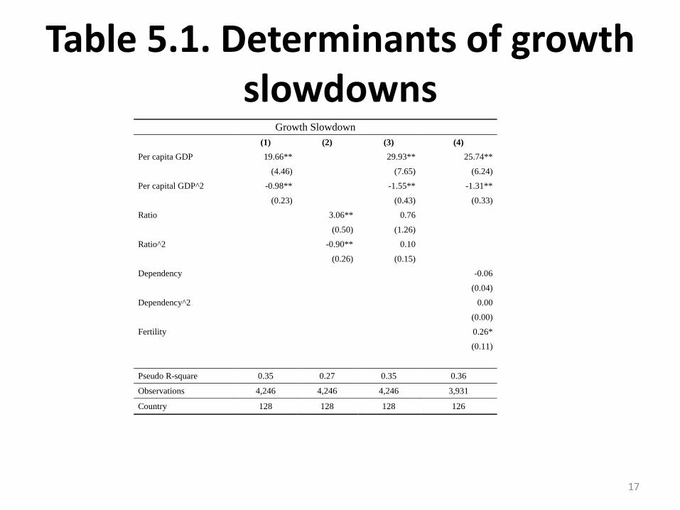
Table 5.1. Determinants of growth slowdowns
17
Growth Slowdown
(1) (2) (3) (4)
Per capita GDP 19.66** 29.93** 25.74**
(4.46) (7.65) (6.24)
Per capital GDP^2 -0.98** -1.55** -1.31**
(0.23) (0.43) (0.33)
Ratio 3.06** 0.76
(0.50) (1.26)
Ratio^2 -0.90** 0.10
(0.26) (0.15)
Dependency -0.06
(0.04)
Dependency^2 0.00
(0.00)
Fertility 0.26*
(0.11)
Pseudo R-square 0.35 0.27 0.35 0.36
Observations 4,246 4,246 4,246 3,931
Country 128 128 128 126
Extensions
• Table 6.1 and 6.2.
• Political regimes, trade openness and financial openness do not seem to matter for slowdowns.
• Higher old age dependency ratios seem to matter more than youth dependency ratios.
• External (terms of trade shocks) matter when interacted with openness.
• Unusually low consumption shares seem to be associated with slowdowns.
18
Effects of economic policy
• Table 7.1, 7.2, 8.1, 8.2
• Slowdowns more likely when:
– Inflation is high
– Exchange rate is undervalued.
• To measure undervaluation we correct the real exchange rate for per capita income (Balassa-Samuelson) and compute deviations from predicted.
19
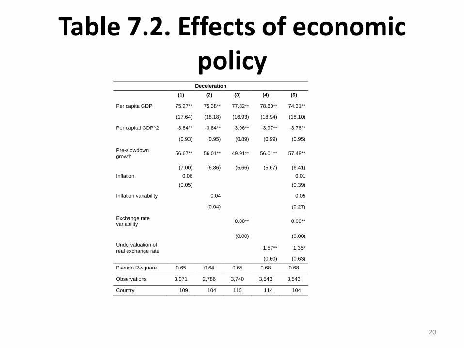
Table 7.2. Effects of economic policy
20
Deceleration
(1) (2) (3) (4) (5)
Per capita GDP 75.27** 75.38** 77.82** 78.60** 74.31**
(17.64) (18.18) (16.93) (18.94) (18.10)
Per capital GDP^2 -3.84** -3.84** -3.96** -3.97** -3.76**
(0.93) (0.95) (0.89) (0.99) (0.95)
Pre-slowdown growth
56.67** 56.01** 49.91** 56.01** 57.48**
(7.00) (6.86) (5.66) (5.67) (6.41)
Inflation 0.06 0.01
(0.05) (0.39)
Inflation variability 0.04 0.05
(0.04) (0.27)
Exchange rate variability
0.00** 0.00**
(0.00) (0.00)
Undervaluation of real exchange rate
1.57** 1.35*
(0.60) (0.63)
Pseudo R-square 0.65 0.64 0.65 0.68 0.68
Observations 3,071 2,786 3,740 3,543 3,543
Country 109 104 115 114 104

Table 8.2 Hazard model of slowdowns
21
Slowdown Hazard
(1) (2) (3) (4) (5)
Inflation 0.321 10.551**
(0.223) (2.377)
Inflation variability
0.103 -9.602**
(0.147) (2.204)
Exchange rate variability
-0.011 0.002
(0.013) (0.002)
Undervaluation of real exchange rate
3.036** 3.038**
(0.942) (1.062)
alpha 4.128** 4.154** 4.107** 4.318** 4.454**
(0.121) (0.125) (0.111) (0.123) (0.155)
Observations 100 93 107 105 92

Undervaluation result is provocative
• Why? Inquiring minds want to know. – It may be that countries that rely on undervalued exchange rates to
boost economic growth are more vulnerable to external shocks resulting in sustained slowdowns.
– It may be that real undervaluation works as a mechanism for boosting growth during the early stages of development when a country relies on shifting labor from agriculture to export-oriented manufacturing but not in subsequent stages when growth becomes more innovation intensive, but governments are reluctant to abandon the earlier policy strategy, leaving the economy increasingly susceptible to slowing down.
– It could be that real undervaluation allows imbalances and excesses in export-oriented manufacturing build up, as in Korea in the 1990s, through that channel making a sustained deterioration in subsequent growth performance more likely.
22
Implications for China
• Recall that they suggest that the probability of a slowdown is highest when per capita GDP reaches $16,740 U.S. (year 2005 international) dollars, when the ratio of per capita income to that in the lead country is 58 per cent, and when the share of employment in manufacturing reaches 23 per cent.
• In Table 3.2 we see that China’s per capita GDP is $8,511 U.S dollars and the ratio of China’s per capita GDP to that in the U.S. is 19.8 per cent in 2007. – If China grows at 9.3 per cent, which is the average growth rate of per
capita GDP for the most recent ten years in the Penn World Table (1998-2007), by 2015 China’s per capita GDP reaches $17,335, just exceeding our slowdown threshold.
– If China grows more modestly at 7 per cent, then per capita GDP reaches the threshold level in 2017.
23

Table 3.2 Slowdown countries and China
24
Obs. Mean Std.
Dev. Min Max
China
2007
China
Average*
China
2007
China
Average*
PWT Version 1 PWT Version 2
Per capita GDP 142 16,740 5,980 10,004 40,614 8,511 5,402 7,868 5,505
Ratio 142 .640 .176 .322 1.109 .198 .134 .183 .136
Dependency 126 54.2 9.0 38.6 73.5 40.4 45.1 40.4 45.1
Old dependency 126 14.8 5.2 6.2 24.3 11.0 10.4 11.0 10.4
Young
dependency 126 39.4 8.6 23.8 61.0 29.4 34.7 29.4 34.7
Trade Openness 142 .843 .900 .093 3.990 .690 .530 .746 .520
Financial
openness 109 .610 1.404 -1.831 2.500 -1.14 -1.14 -1.14 -1.14
Growth of Terms
of trade 125 -.010 .060 -.224 .176 -.025 -.033 -.025 -.033
Positive political
change 124 .145 .354 0 1 0 0 0 0
Negative political
change 124 .073 .260 0 1 0 0 0 0
Consumption
share of GDP 142 .535 .092 .327 .851 .375 .440 .365 .443
Investment share
of GDP 142 .346 .093 .159 .584 .324 .313 .313 .316
Government
share of GDP 142 .125 .064 .039 .405 .202 .223 .214 .217
Aggregate GDP
Growth Rate 142 .064 .033 -.079 .143 .140 .099 .104 .084
Capital
Contribution to
GDP Growth
121 .026 .009 .010 .053
(142) (.025) (.011) (.009) (.048) (.040) (.034) (.040) (.034)
Employment
Contribution to
GDP Growth
120 .009 .006 -.002 .033
(141) (.009) (.006) (-.004) (.027) (.007) (.009) (.007) (.009)
Human Capital
Contribution to
GDP Growth
121 .005 .003 -.001 .013
(132) (.005) (.003) (-.001) (.012) (.005) (.006) (.005) (.006)
TFP Contribution
to GDP Growth
120 .025 .028 -.099 .086
(131) (.023) (.027) (-.107) (.080) (.088) (.051) (.052 ) (.036)

Implications for China
• China’s share of manufacturing in total employment was 11.3 per cent in 2002, the latest year for which data are available.
• In the absence of further figures we assume that this fraction has been growing at one per cent per annum. If this is right, it suggests that the share of employment in manufacturing is now within hailing distance of the 23 per cent where historical comparisons suggest that growth slows down.
• Our results further suggest that the fact that Chinese growth has been unusually fast, that its growth has been associated with what is widely viewed as a chronically undervalued exchange rate, that the old-age dependency ratio is rising, and that the consumption share of GDP is exceptionally low heightens the likelihood of an imminent slowdown
25

Implications for China
• We can use a selection of our estimated equations together with 2007 values of the independent variables to estimate the likelihood of a Chinese slowdown.
• Using the coefficients in Table 6.2, columns 6 and 13, where the key independent variables are per capita income, the pre-slowdown rate of growth, demographic structure (in column 6) and trade openness and the composition of spending (in column 13) puts the probability at 77 and 73 per cent.
• Table 7.2, column 5, where the independent variables are policy measures (inflation, inflation variability and real undervaluation), this procedure puts the probability of a slowdown at 71 per cent. – These are non-negligible odds.
26


