
Web Data Preprocessing
Department of Communication PhD Student Workshop Web Mining for Communication Research
April 22-25, 2014
http://weblab.com.cityu.edu.hk/blog/project/workshops
Zhenzhen Wang
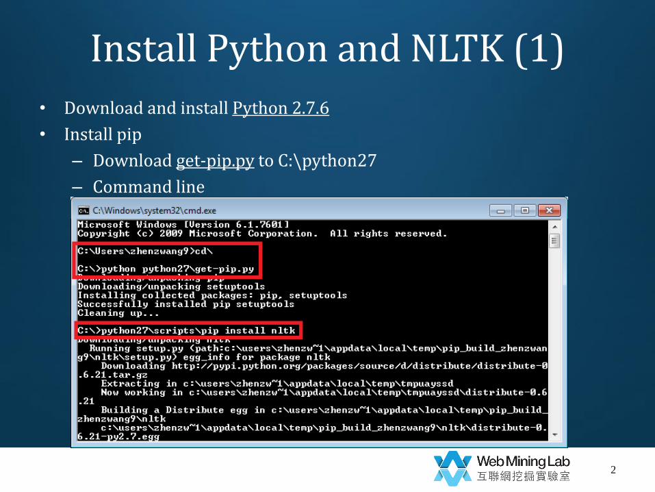
Install Python and NLTK (1)
• Download and install Python 2.7.6
• Install pip
– Download get-pip.py to C:\python27
– Command line
2
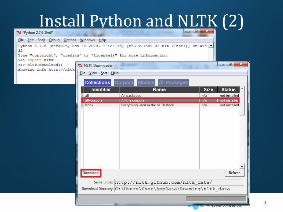
Install Python and NLTK (2)
3
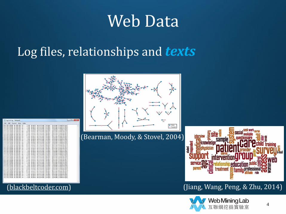
Web Data
Log files, relationships and texts
4
(Jiang, Wang, Peng, & Zhu, 2014)
(Bearman, Moody, & Stovel, 2004)
(blackbeltcoder.com)

Web Data Preprocessing
5
Tokenization
Dropping common terms
Normalization
Stemming/ lemmatization
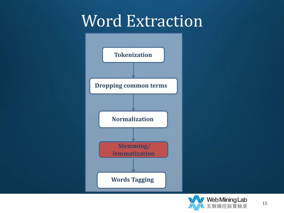
Word Extraction
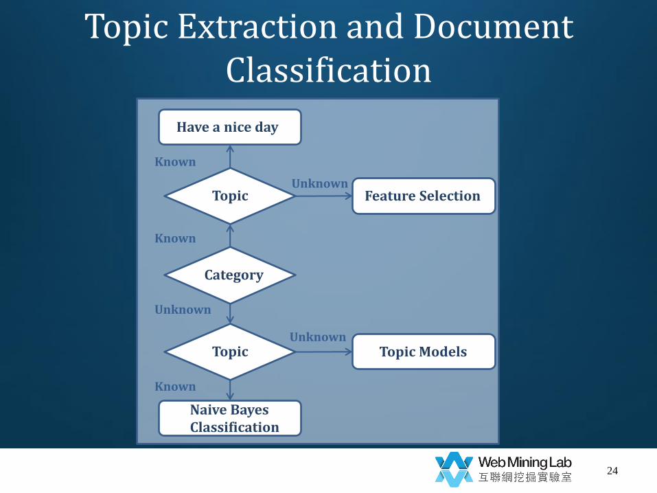
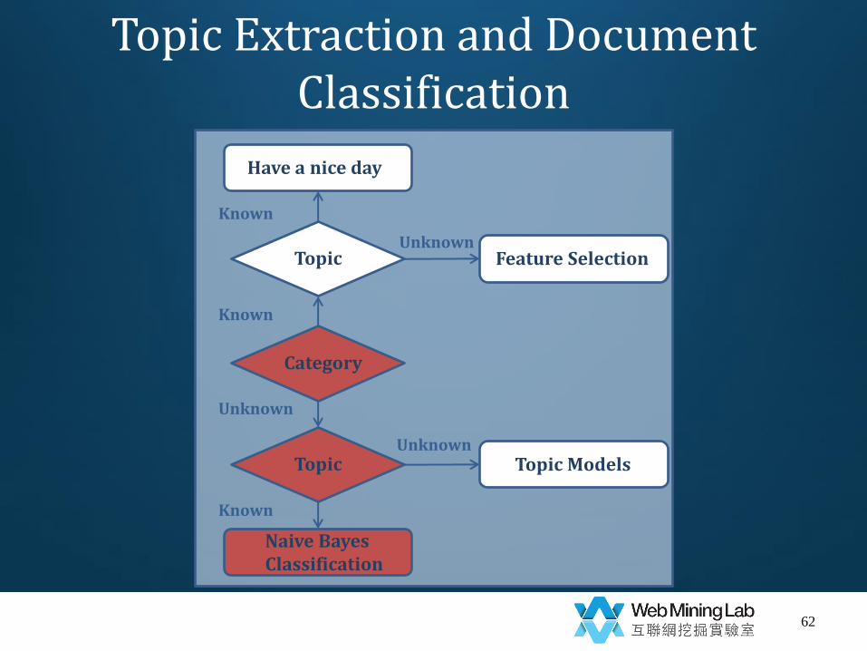
Category
Topic
Topic Topic Models
Naive Bayes Classification
Feature Selection
Have a nice day
Known
Known
Unknown
Unknown
Unknown
Known
Topic Extraction and Document Classification
Words Tagging

Word Extraction
6
Tokenization
Dropping common terms
Normalization
Stemming/ lemmatization
Words Tagging
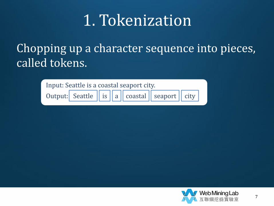
1. Tokenization
Chopping up a character sequence into pieces, called tokens.
7
Input: Seattle is a coastal seaport city.
Output: Seattle is a coastal seaport city

Word Extraction
8
Tokenization
Dropping common terms
Normalization
Stemming/ lemmatization
Words Tagging
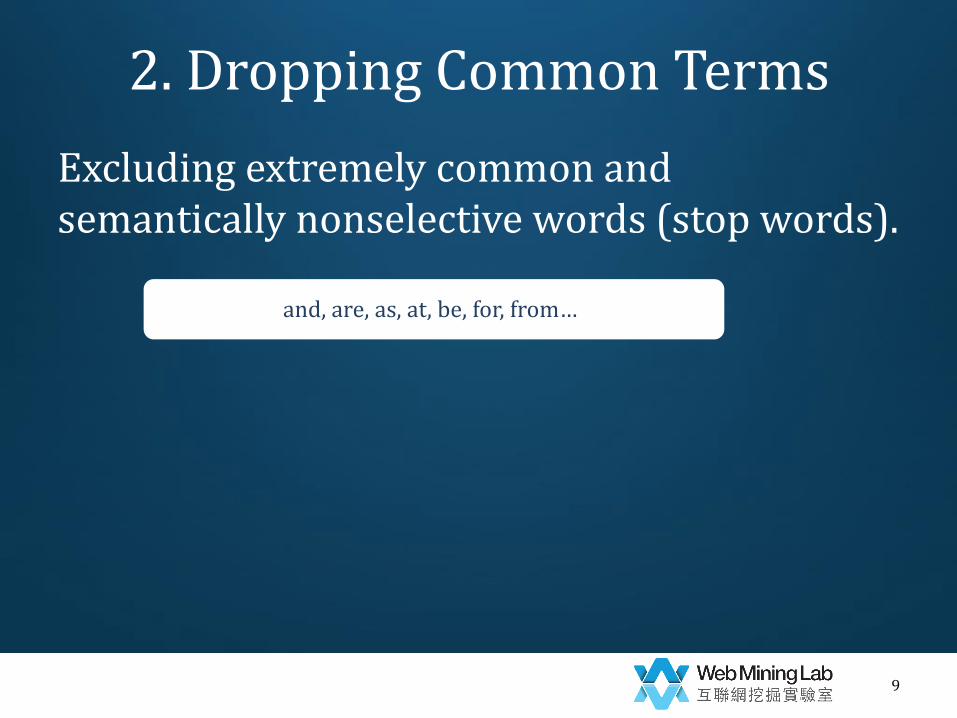
2. Dropping Common Terms
Excluding extremely common and semantically nonselective words (stop words).
9
and, are, as, at, be, for, from…
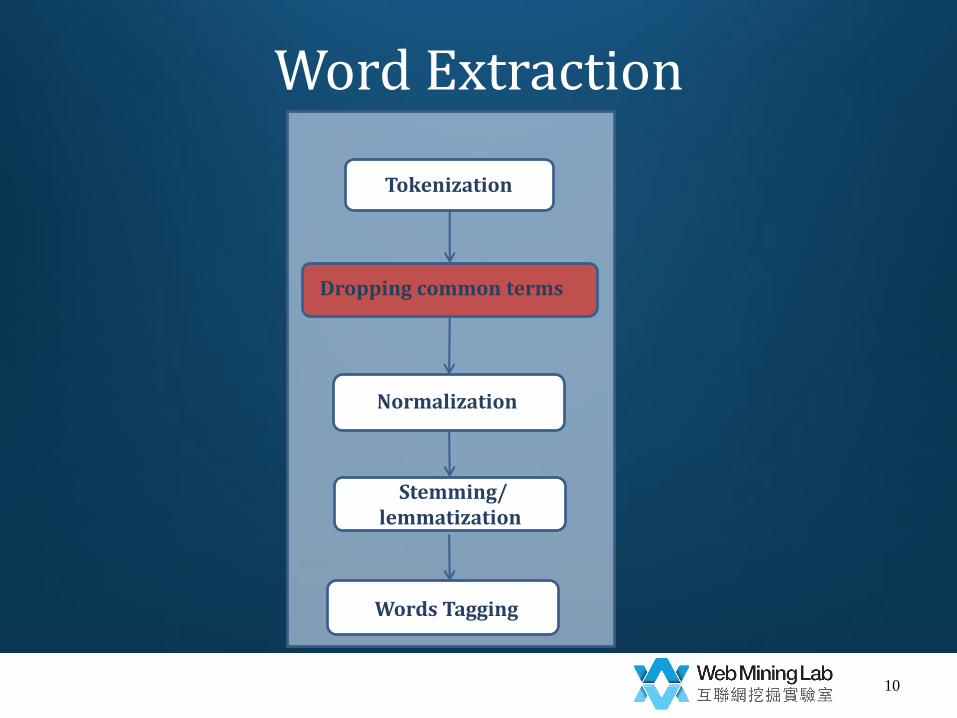
Word Extraction
10
Tokenization
Dropping common terms
Normalization
Stemming/ lemmatization
Words Tagging
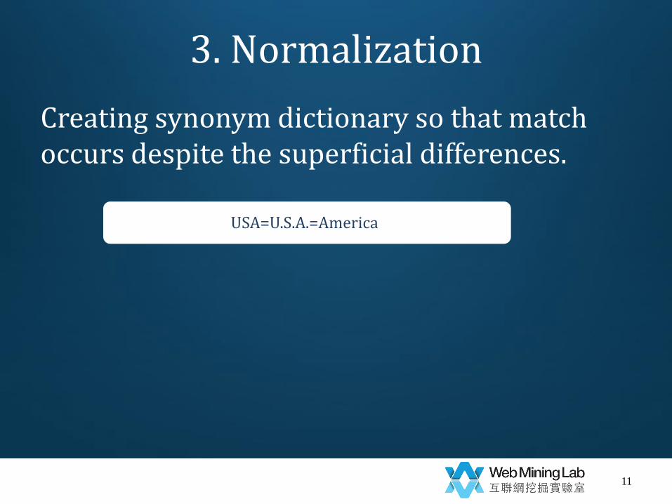
3. Normalization
Creating synonym dictionary so that match occurs despite the superficial differences.
11
USA=U.S.A.=America
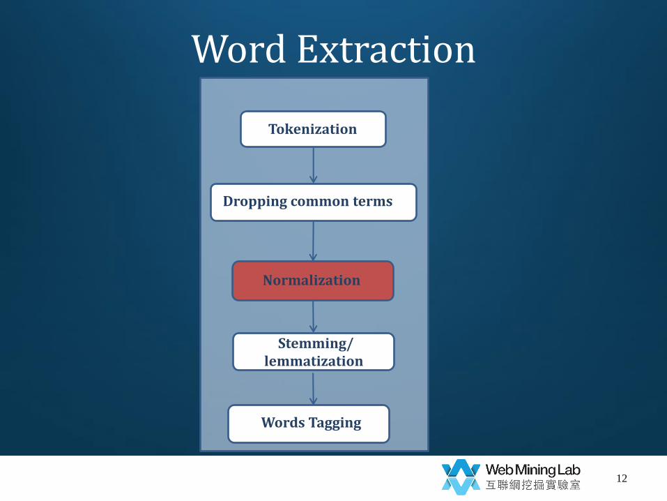
Word Extraction
12
Tokenization
Dropping common terms
Normalization
Stemming/ lemmatization
Words Tagging
4. Stemming and Lemmatization: Aim
Reducing related forms of a word to a common base form.
13
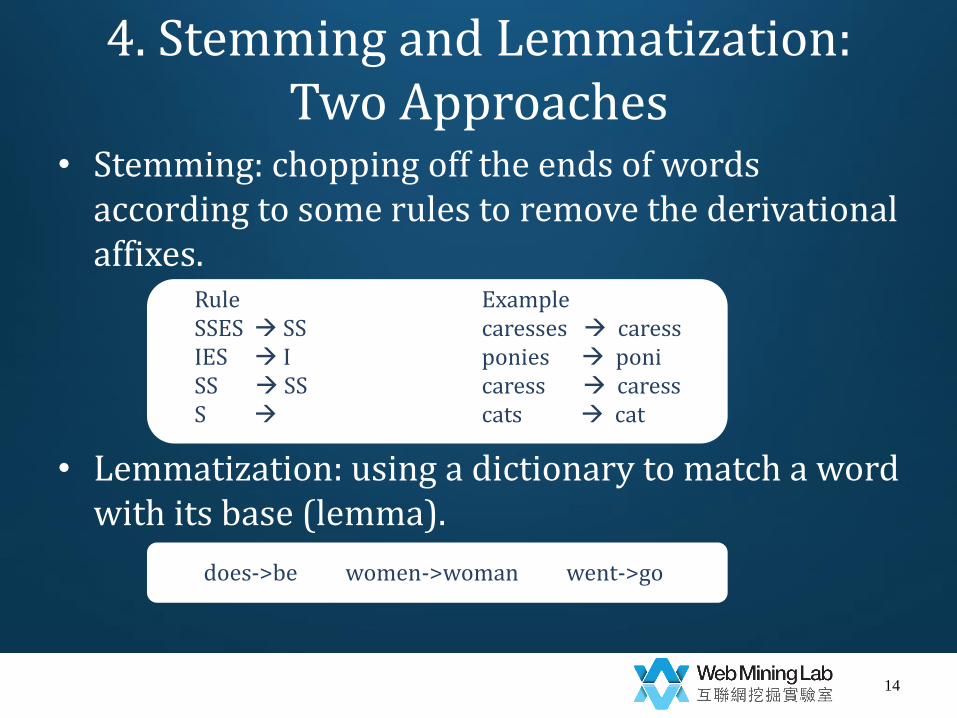
4. Stemming and Lemmatization: Two Approaches
• Stemming: chopping off the ends of words according to some rules to remove the derivational affixes.
• Lemmatization: using a dictionary to match a word with its base (lemma).
14
does->be women->woman went->go
Rule Example SSES SS caresses caress IES I ponies poni SS SS caress caress S cats cat
Word Extraction
15
Tokenization
Dropping common terms
Normalization
Stemming/ lemmatization
Words Tagging
5. Words Tagging: Aim
Marking up a word, based on both its definition, as well as its context, often requiring context-specific dictionaries.
16
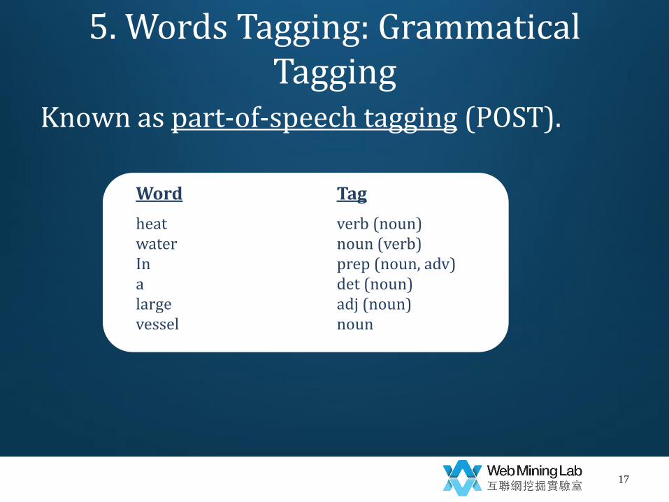
5. Words Tagging: Grammatical Tagging
Known as part-of-speech tagging (POST).
17
Word Tag
heat verb (noun) water noun (verb) In prep (noun, adv) a det (noun) large adj (noun) vessel noun
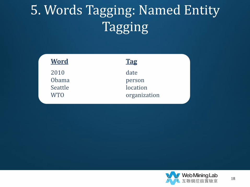
5. Words Tagging: Named Entity Tagging
18
Word Tag
2010 date Obama person Seattle location WTO organization

5. Words Tagging: Sentimental Tagging
19
Word Tag
love positive dazzling positive suck negative still neutral wonderful positive waste negative

Demo 1: Online Tool for Word Extraction
• Open Xerox
20
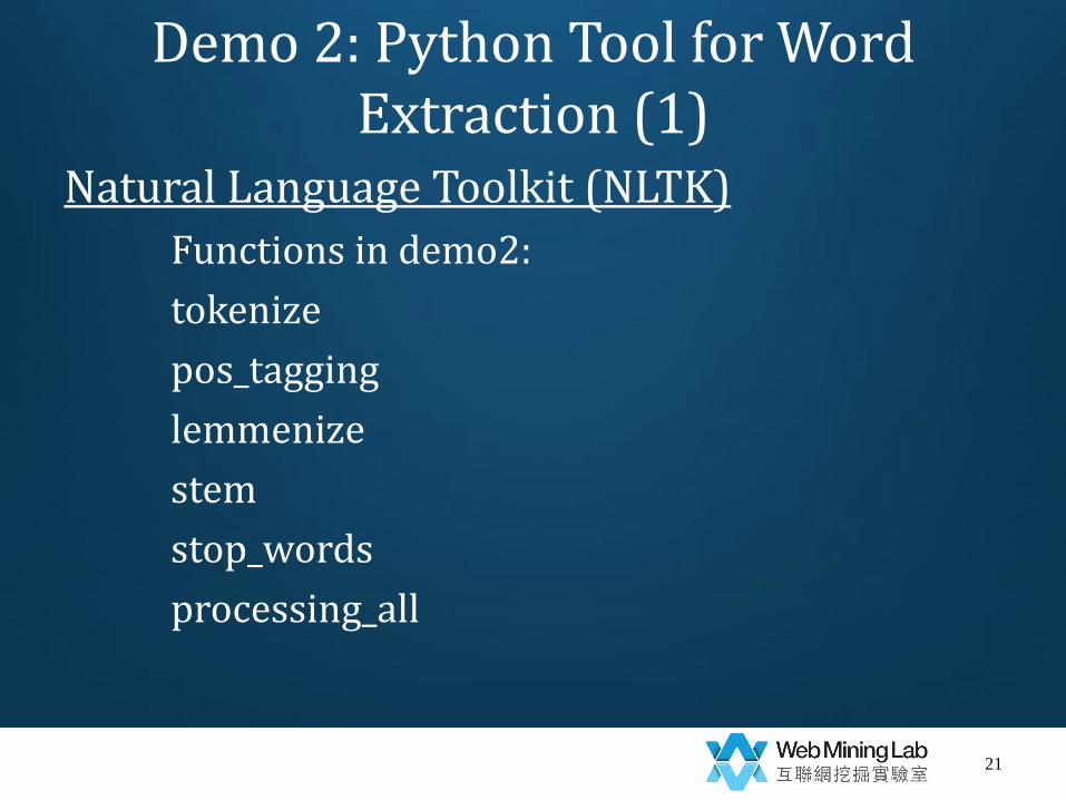
Demo 2: Python Tool for Word Extraction (1)
Natural Language Toolkit (NLTK)
Functions in demo2:
tokenize
pos_tagging
lemmenize
stem
stop_words
processing_all
21
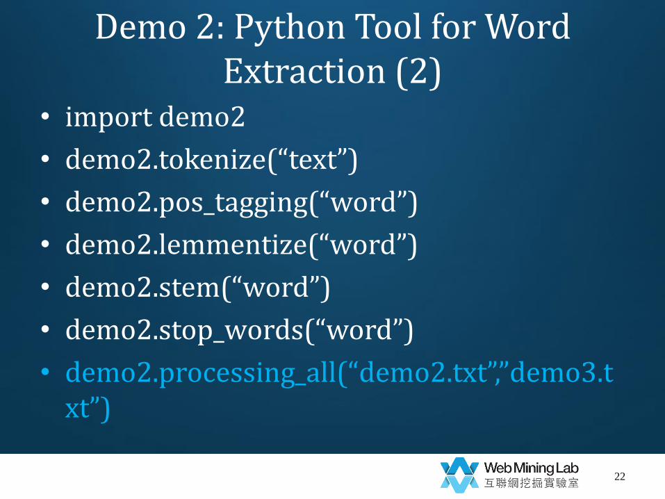
Demo 2: Python Tool for Word Extraction (2)
• import demo2
• demo2.tokenize(“text”)
• demo2.pos_tagging(“word”)
• demo2.lemmentize(“word”)
• demo2.stem(“word”)
• demo2.stop_words(“word”)
• demo2.processing_all(“demo2.txt”,”demo3.txt”)
22

Demo 2: Python Tool for Word Extraction (3)
23
24
Category
Topic
Topic Topic Models
Naive Bayes Classification
Feature Selection
Have a nice day
Known
Known
Unknown
Unknown
Unknown
Known
Topic Extraction and Document Classification
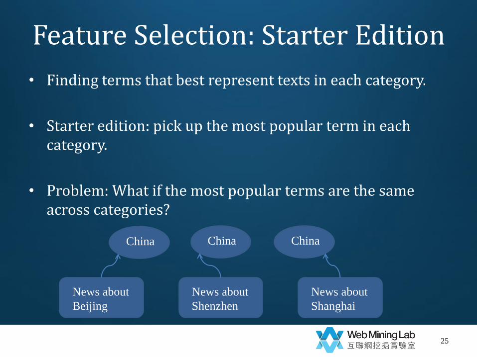
Feature Selection: Starter Edition
• Finding terms that best represent texts in each category.
• Starter edition: pick up the most popular term in each category.
• Problem: What if the most popular terms are the same across categories?
25
News about
Beijing
News about
Shenzhen
News about
Shanghai
China China China

Feature Selection: Advanced Edition
• Picking up the most discriminant terms in each category.
• χ2 calculates whether the occurrence of the term and occurrence of the category are independent.
26
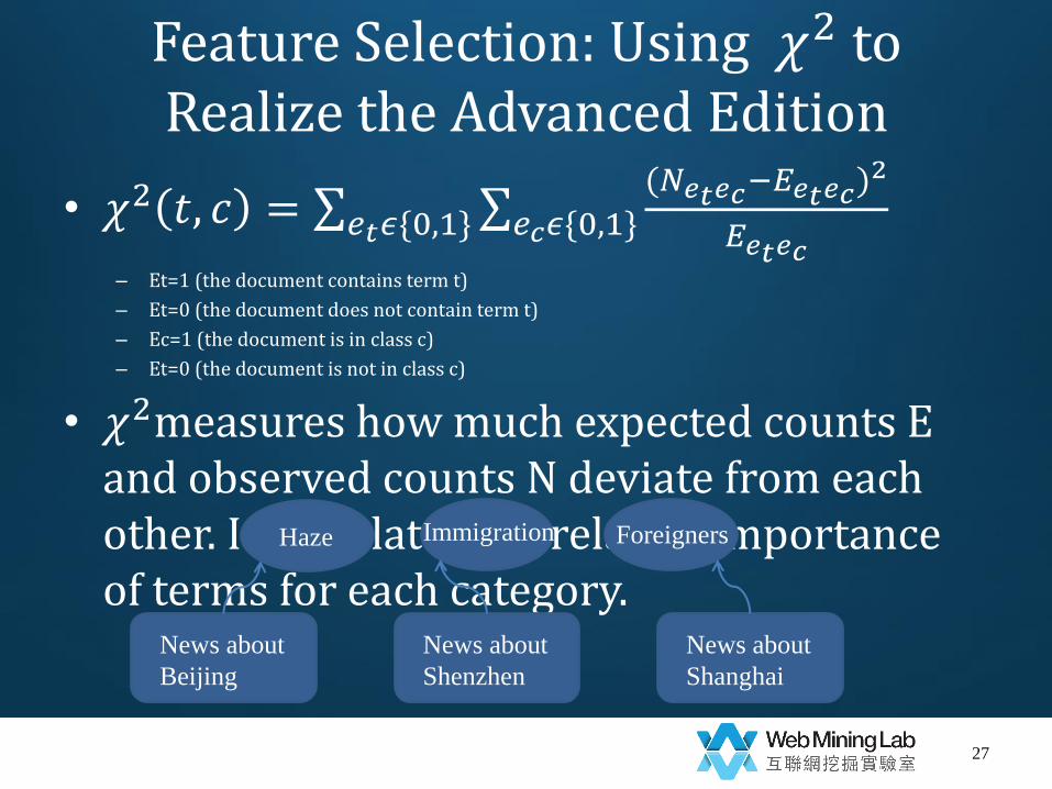
Feature Selection: Using 𝜒2 to Realize the Advanced Edition
• 𝜒2 𝑡, 𝑐 = (𝑁𝑒𝑡𝑒𝑐
−𝐸𝑒𝑡𝑒𝑐)2
𝐸𝑒𝑡𝑒𝑐𝑒𝑐𝜖{0,1}𝑒𝑡𝜖{0,1}
– Et=1 (the document contains term t)
– Et=0 (the document does not contain term t)
– Ec=1 (the document is in class c)
– Et=0 (the document is not in class c)
• 𝜒2measures how much expected counts E and observed counts N deviate from each other. It calculates the relative importance of terms for each category.
27
News about
Beijing
News about
Shenzhen
News about
Shanghai
Haze Immigration Foreigners
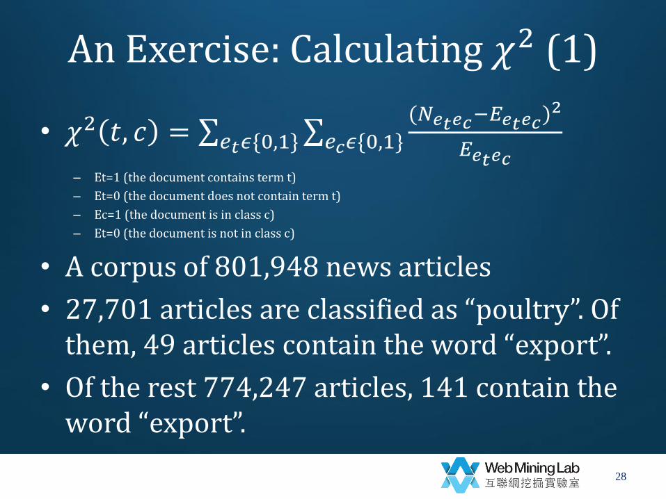
An Exercise: Calculating 𝜒2 (1)
• 𝜒2 𝑡, 𝑐 = (𝑁𝑒𝑡𝑒𝑐
−𝐸𝑒𝑡𝑒𝑐)2
𝐸𝑒𝑡𝑒𝑐𝑒𝑐𝜖{0,1}𝑒𝑡𝜖{0,1}
– Et=1 (the document contains term t)
– Et=0 (the document does not contain term t)
– Ec=1 (the document is in class c)
– Et=0 (the document is not in class c)
• A corpus of 801,948 news articles
• 27,701 articles are classified as “poultry”. Of them, 49 articles contain the word “export”.
• Of the rest 774,247 articles, 141 contain the word “export”.
28
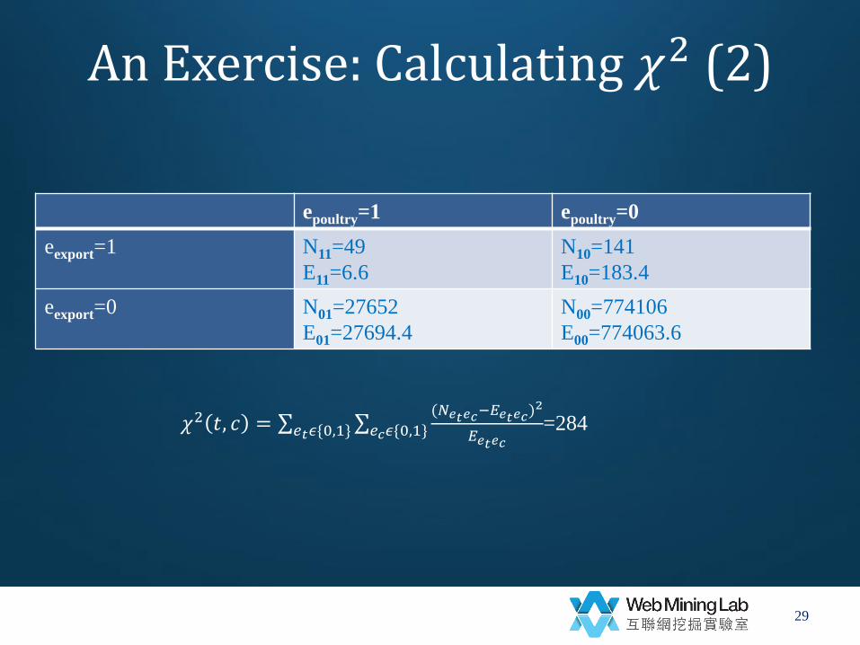
An Exercise: Calculating 𝜒2 (2)
epoultry=1 epoultry=0
eexport=1 N11=49
E11=6.6
N10=141
E10=183.4
eexport=0 N01=27652
E01=27694.4
N00=774106
E00=774063.6
29
𝜒2 𝑡, 𝑐 = (𝑁𝑒𝑡𝑒𝑐
−𝐸𝑒𝑡𝑒𝑐)2
𝐸𝑒𝑡𝑒𝑐𝑒𝑐𝜖{0,1}𝑒𝑡𝜖{0,1}
=284
• Data: 225 pieces of economic news from Reuters (51 about China, 174 about Japan).
• RQ: What’s the focus of Reuters for each country?
30
Demo 3: Use SPSS to Do Feature Selection
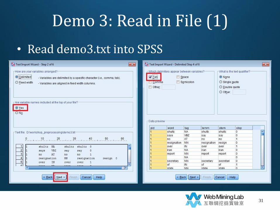
Demo 3: Read in File (1)
• Read demo3.txt into SPSS
31
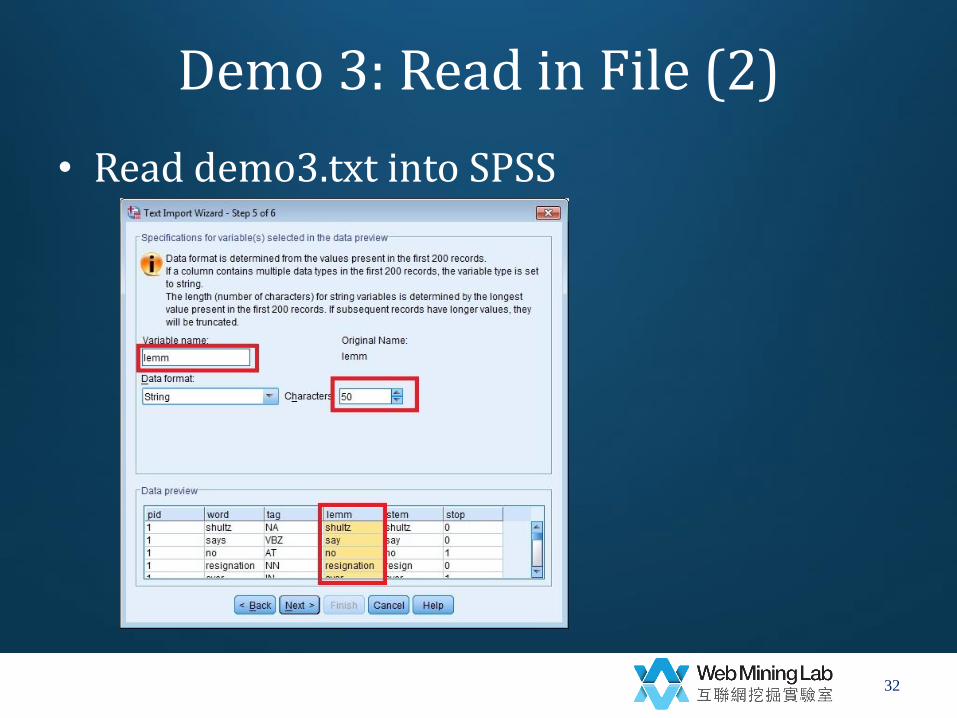
Demo 3: Read in File (2)
• Read demo3.txt into SPSS
32
Demo 3: Select Words(1)
• Filter out stop words and spaces
– Data->
– Select cases->
• stop=0 and word~=" "
• Delete unselected cases
33

Demo 3: Select Words(2)
34

Demo 3: Select Words(3)
35

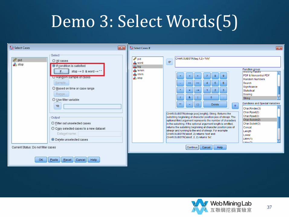
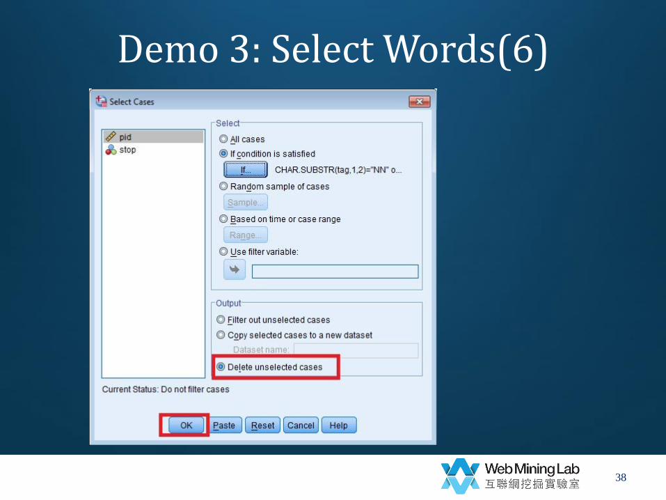
Demo 3: Select Words(4)
• Select nouns only
– Data->
– Select cases->
• CHAR.SUBSTR(tag,1,2)="NN" or CHAR.SUBSTR(tag,1,2)="NA"
• Delete unselected cases
36
Demo 3: Select Words(5)
37
Demo 3: Select Words(6)
38

Demo 3: Calculate Term Frequency (Prepare for Demo 4) (1)
• Calculate term frequency
– Data->
– Aggregate->
• break variables=pid & lemm
• Number of cases=tf
• Create a new dataset containing only the aggregated variables
• Save the file as “demo4.sav”
39

Demo 3: Calculate Term Frequency (Prepare for Demo 4) (2)
40
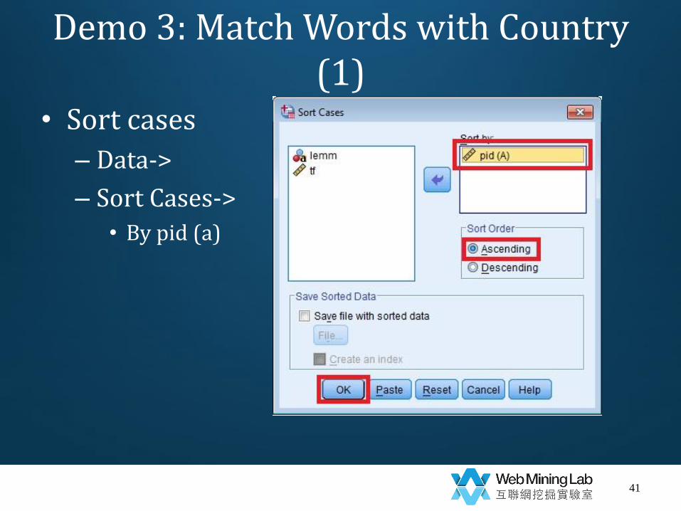
Demo 3: Match Words with Country (1)
• Sort cases
– Data->
– Sort Cases->
• By pid (a)
41

Demo 3: Match Words with Country (2)
• Match words with country
– Data->
– Merge Files->
– Add Variables->
– Merge with “demo2.sav”
• Key variable=pid
• Non-active data set is keyed table
• Exclude variable=news tf
42
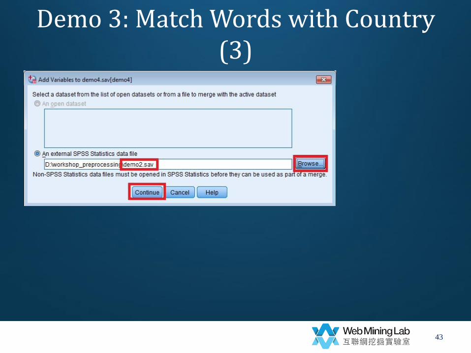
Demo 3: Match Words with Country (3)
43
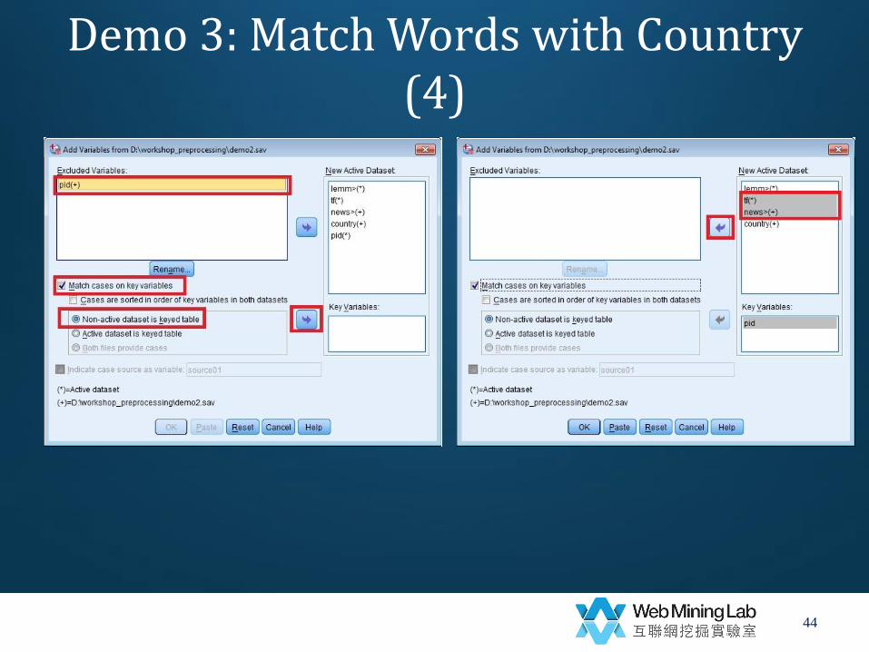
Demo 3: Match Words with Country (4)
44
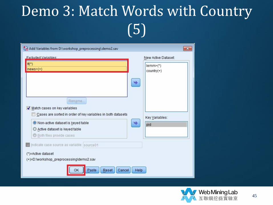
Demo 3: Match Words with Country (5)
45
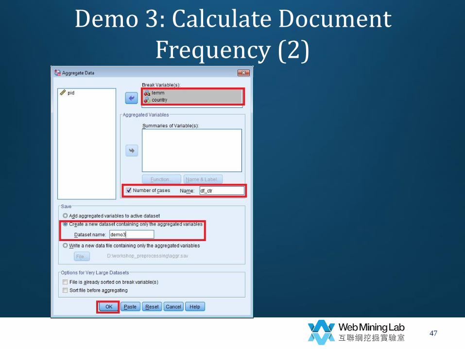
Demo 3: Calculate Document Frequency (1)
• Calculate document frequency for each country
– Data->
– Aggregate->
• break variables=lemm & country
• Number of cases=df_ctr
• Create a new dataset containing only the aggregated variables
• Dataset name: demo3
46
Demo 3: Calculate Document Frequency (2)
47
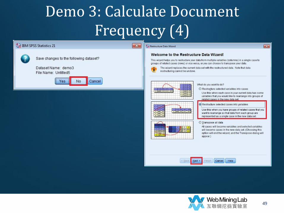
Demo 3: Calculate Document Frequency (3)
• Transform long data to wide data
– Data->
– Reconstructure ->
– Reconstructure selected cases into variables->
• Identified variables=lemm
• Index variables=country
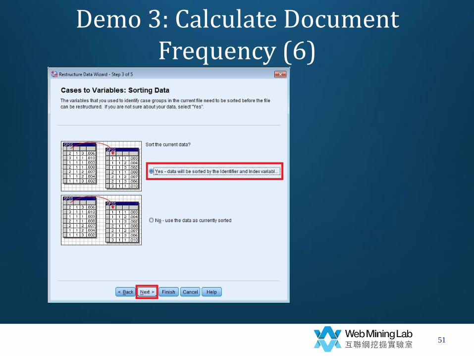
• Sort
• Group by original values
48
Demo 3: Calculate Document Frequency (4)
49

Demo 3: Calculate Document Frequency (5)
50
Demo 3: Calculate Document Frequency (6)
51
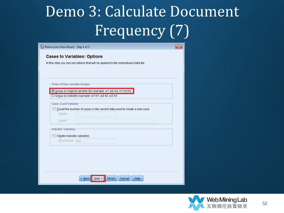
Demo 3: Calculate Document Frequency (7)
52
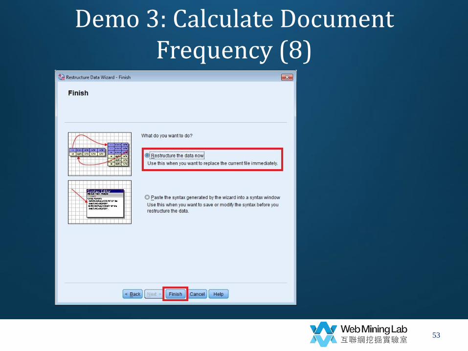
Demo 3: Calculate Document Frequency (8)
53
Demo 3: Calculate Document Frequency (9)
• Add missing values
– Transform->
– Compute Variables->
• df_ctr.1=0
• if (include if cases satisfied condition) MISSING(df_ctr.1)
54
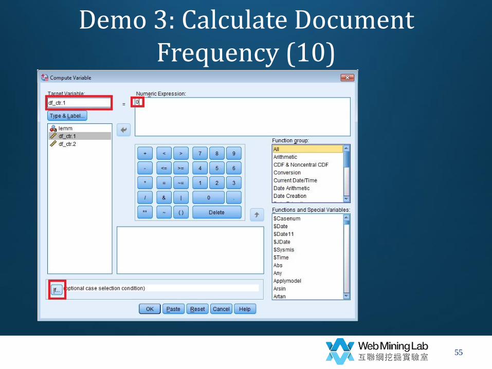
Demo 3: Calculate Document Frequency (10)
55
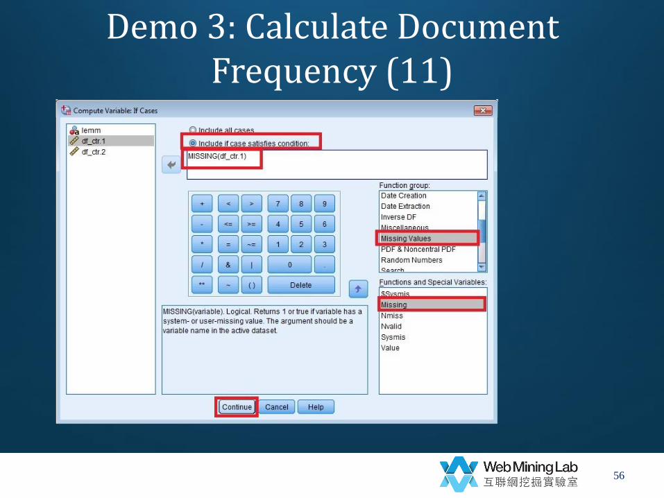
Demo 3: Calculate Document Frequency (11)
56

Demo 3: Calculate χ2 • Compute expected values
– Transform-> – Compute Variables->
• N11=df_ctr.1 • N10=df_ctr.2 • E11=(df_ctr.1+df_ctr.2)*(51/225) • E10=(df_ctr.1+df_ctr.2)*(174/225) • N01=51-df_ctr.1 • N00=174-df_ctr.2 • E01=N11+N01-E11 • E00=N10+N00-E10
• Compute χ2
– Transform-> – Compute Variables->
• kai=(N11-E11)**2/E11+(N11-E10)**2/E10+(N11-E01)**2/E01+(N11-E00)**2/E00+ (N10-E11)**2/E11+(N10-E10)**2/E10+(N10-E01)**2/E01+(N10-E00)**2/E00+ (N01-E11)**2/E11+(N01-E10)**2/E10+(N01-E01)**2/E01+(N01-E00)**2/E00+ (N00-E11)**2/E11+(N00-E10)**2/E10+(N00-E01)**2/E01+(N00-E00)**2/E00
57

Demo 3: Select Words
• Sort by χ2
– Data-> – Sort Cases->
• By kai (D)
• Filter out rare words – Data-> – Select cases->
• (df_ctr.1+df_ctr.2)>=7 • Delete unselected cases
• Compute expected values – Transform-> – Compute Variables->
• portion1=df_ctr.1/51 • portion2=df_ctr.2/174
58
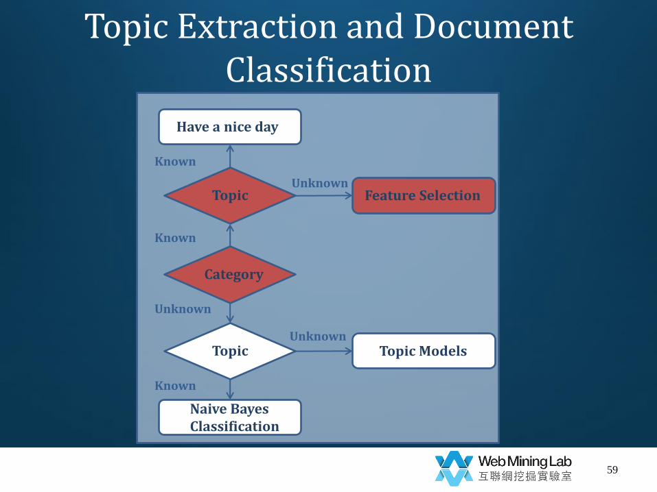
Topic Extraction and Document Classification
59
Category
Topic
Topic Topic Models
Naive Bayes Classification
Feature Selection
Have a nice day
Known
Known
Unknown
Unknown
Unknown
Known
Naive Bayes (NB) Classification: Process
1. Retrieving a training set (usually manually), with texts already assigned to a known list of categories.
2. Based on the training set, determining the contribution of each term for each category.
3. Based on the terms in texts, assigning new texts into categories.
60
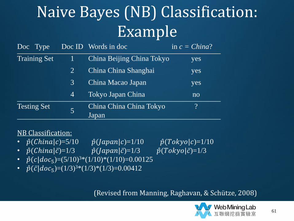
Naive Bayes (NB) Classification: Example
61
(Revised from Manning, Raghavan, & Schütze, 2008)
Doc Type Doc ID Words in doc in c = China?
Training Set 1 China Beijing China Tokyo yes
2 China China Shanghai yes
3 China Macao Japan yes
4 Tokyo Japan China no
Testing Set 5
China China China Tokyo
Japan
?
NB Classification: • 𝑝 (𝐶ℎ𝑖𝑛𝑎|𝑐)=5/10 𝑝 (𝐽𝑎𝑝𝑎𝑛|𝑐)=1/10 𝑝 (𝑇𝑜𝑘𝑦𝑜|𝑐)=1/10 • 𝑝 (𝐶ℎ𝑖𝑛𝑎|𝑐 )=1/3 𝑝 (𝐽𝑎𝑝𝑎𝑛|𝑐 )=1/3 𝑝 (𝑇𝑜𝑘𝑦𝑜|𝑐 )=1/3
• 𝑝 (𝑐|𝑑𝑜𝑐5)=(5/10)3*(1/10)*(1/10)=0.00125
• 𝑝 (𝑐 |𝑑𝑜𝑐5)=(1/3)3*(1/3)*(1/3)=0.00412
Topic Extraction and Document Classification
62
Category
Topic
Topic Topic Models
Naive Bayes Classification
Feature Selection
Have a nice day
Known
Known
Unknown
Unknown
Unknown
Known

Topic Models: Assumptions
• Documents are mixtures of topics, where a topic is a probability distribution over words.
63
(Steyvers & Griffiths, 2007)
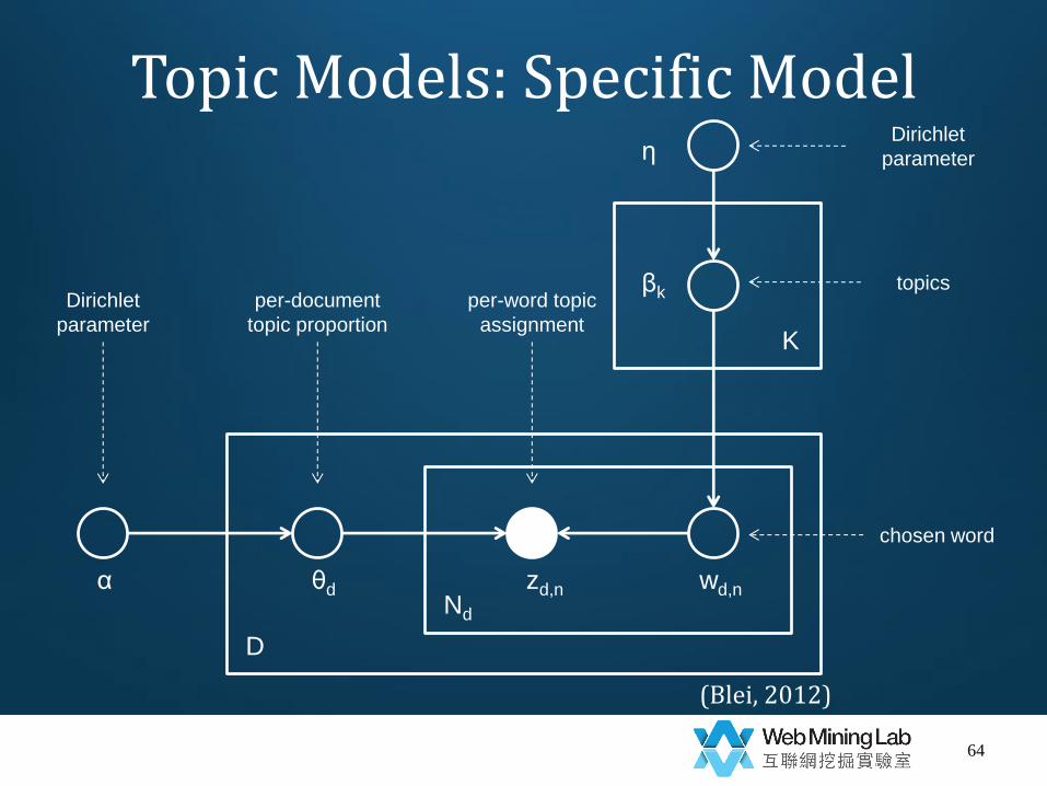
Topic Models: Specific Model
64
(Blei, 2012)
zd,n wd,n θd
βk
α
η
D
Nd
K
Dirichlet
parameter
per-document
topic proportion
per-word topic
assignment
chosen word
topics
Dirichlet
parameter
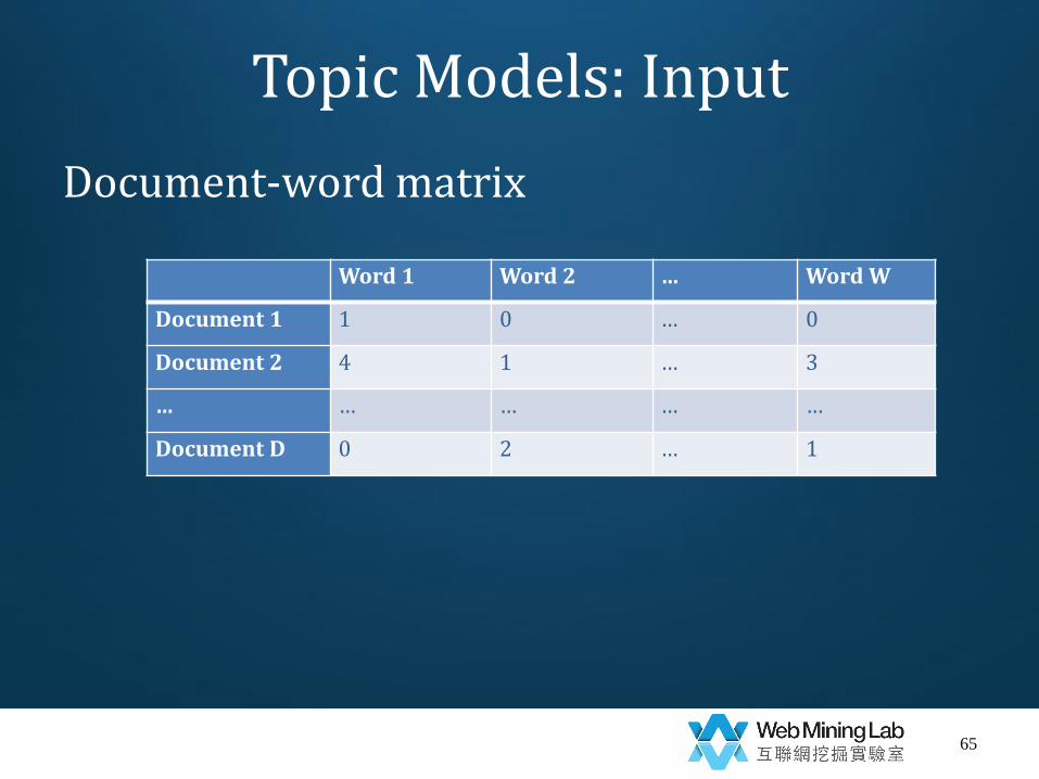
Topic Models: Input
Document-word matrix
65
Word 1 Word 2 … Word W
Document 1 1 0 … 0
Document 2 4 1 … 3
… … … … …
Document D 0 2 … 1
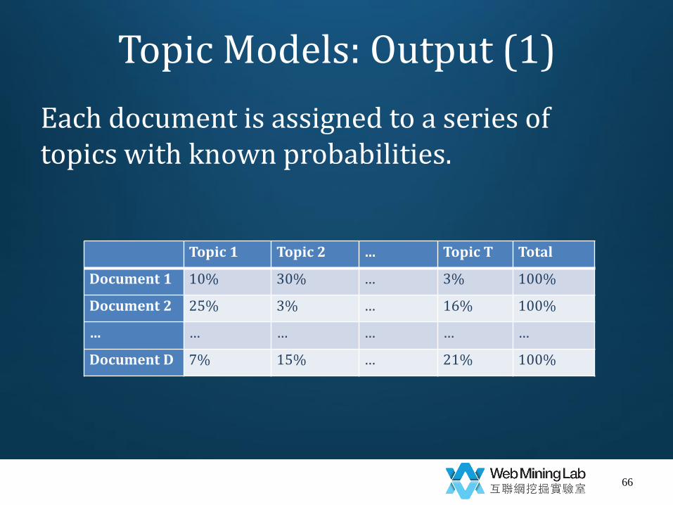
Topic Models: Output (1)
Each document is assigned to a series of topics with known probabilities.
66
Topic 1 Topic 2 … Topic T Total
Document 1 10% 30% … 3% 100%
Document 2 25% 3% … 16% 100%
… … … … … …
Document D 7% 15% … 21% 100%

Topic Models: Output (2)
Each topic is composed of a series of words with known probabilities.
67
Word 1 Word 2 … Word W Total
Topic 1 1% 6% … 3% 100%
Topic 2 2% 3% … 8% 100%
… … … … … …
Topic T 9% 15% … 2% 100%
Demo 4: Use SPSS to Prepare Data for Topic Models
• Data: 225 Reuters news stories
• Task: generate a document-word matrix
68

Demo 4: Load File and Select Words
• Load “demo4.sav” • Filter out rare words
– Data-> – Aggregate->
• break variables=lemm • Number of cases=df • Create a new dataset containing only the aggregated
variables • Add aggregated variables to active dataset
– Data-> – Select cases->
• df>=10 • Delete unselected cases
69
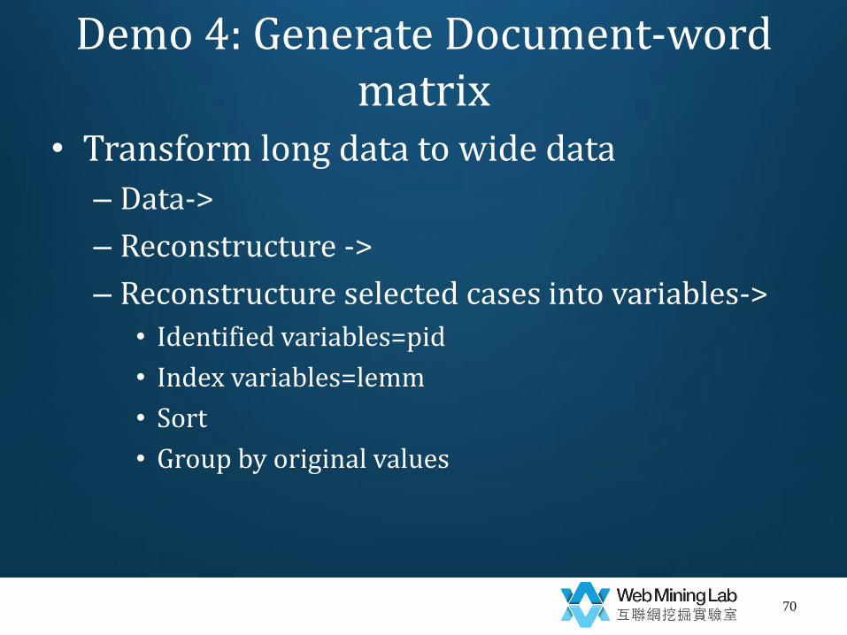
Demo 4: Generate Document-word matrix
• Transform long data to wide data
– Data->
– Reconstructure ->
– Reconstructure selected cases into variables->
• Identified variables=pid
• Index variables=lemm
• Sort
• Group by original values
70

TOOLS
71
List of Tools
• Word Extraction – R tm
– Python NLTK
• Feature selection – Any statistical software capable of calculating
frequency
• Naive Bayes classification: – R e1071
• Topic modeling – R topicmodels
72


