
Weak Cartels and Collusion-Proof Auctions
Yeon-Koo Che∗ Daniele Condorelli† Jinwoo Kim‡
August 13, 2010
Abstract
We study the problem of collusion in private value auctions by cartels whose
members cannot exchange monetary transfers among themselves (i.e. weak cartels).
We restrict attention to a large class of auctions that includes standard auctions,
which we call “winner-payable auctions”. Restricting attention to winner payable
auctions, we provide a complete characterization of collusion-proof auctions. We show
that an auction is collusion-proof if and only if each bidder’s equilibrium probability
of winning the object is constant whenever the value of that bidder lies in an interval
of his type-space, in which the ex-ante distribution of values is convex. Using this
characterization, we are able to identify the optimal collusion-proof auctions for a
broad class of value distributions.
1 Introduction
Collusion is a pervasive problem in auctions. Particularly so in the auctioning of pro-
curement contracts. Despite (or perhaps because of) the increasing use of incentives for
whistleblowing and defection, many cases of bidding irregularities came to light in recent
∗Economics Department, Columbia University, and YERI, Yonsei University†MEDS Department, Northwestern University and Department of Economics, University of Essex‡School of Economics, Yonsei University.
1

years.1 In the UK, the Office of Fair Trading (OFT) alleged 240 cases of bid-rigging in
contracts for building schools, hospitals and universities, involving the country’s biggest
construction firms, with the estimated loss of more than 300 million pounds to taxpayers.2
The Dutch Construction cartel, whose revelation became a TV documentary as well as
one of the biggest financial scandals in the Netherlands, allegedly involved 3,500 rigged
bids and annual overcharges of 500million euros during 1986-1998.3 In the US, bid rigging
accounts for 75% of the antitrust cases (Krishna, 2009).
Many bid-rigging cases fall into the category of what McAfee and McMillan labeled
weak cartels, namely cartels that do not involve exchange of side payments among cartel
members.4 For instance, the most common cartel practices uncovered by OFT were “cover
pricing,” “bid suppression” and “bid rotation”. Cover pricing in procurement occurs when
a bidder posts an artificially inflated bid to generate a false impression of competition. In
bid rotation, members of a cartel take turns, according to some predetermined order, to win
with the auction, with the other bidders refraining from competing aggressively.5 Market
sharing is another typical form collusion without side-payments. In the construction of
Subway Line 7 in Seoul, six different major companies won six different sections of the
subway line construction and they also each submitted six different losing (cover) bids for
the others.
Cartels have good reasons to avoid side payments: monetary transfers leave a trail
of evidence that can expose a cartel and lead to its prosecution. Compensating losing
bidders in money can also lure “pretenders” who join a cartel solely to collect “the loser
compensation” without ever intending to win. At the same time, it is not clear how
1The reward for whistle-blowers are being instituted as a system of encouraging employees and partici-
pants to expose contracts fraud. Leniency programs offer reduce penalties for the firms that come forward
early in exchange for aiding prosecution.2See “Construction cartel may have cost taxpayer 300 million pounds,” Apr 17, 2008, Telegraph.co.uk.3In 2001, a TV program, Zembla, made an investigative report on fraud inquiries in Netherlands. See
Doree (2004).4The cartel is called a strong cartel when its members exchange side payments. See McAfee and
McMillan (1992).5Monetary payment to losers was much less common (...). Compensation to losers was quite rampant
in the Dutch construction cartel, but the compensation was typically a fixed amount, so it is unlikely to
have served the purpose of mediating “efficient” selection of a winning bidder, a feature often associated
with strong cartel.
2

cartel may successfully operate without employing monetary transfers. After all, members
agreeing to lose must be compensated, and compensating in nonmonetary forms entails
efficiency loss. For instance, Pesendorfer (2000)’s study of Texas School Milk Supply cartel
suggests that the sharing of the market among cartel members may not have been adjusted
based on their realized costs. Several questions arise: can weak cartels form and operate
effectively? If so, under what circumstances and what auction formats? What are their
effects? How should auctions be designed to deter weak cartels? We answer these questions.
Our analysis begins where the seminal contribution by McAfee and McMillan (1992;
henceforth MM) left off. They were the first to recognize that weak cartels can operate
successfully, even with extreme allocative inefficiencies. They showed in a model of first-
price auction that bidders with symmetrically distributed values will benefit from agreeing
ex-ante to a completely random assignment of the good at a reserve price, if their com-
mon distribution function exhibits an increasing hazard rate. We follow their modeling
framework, but we advance the analysis in several ways.
First, we consider a more general class of auctions called “winner-payable auctions.”
These are the auctions in which bidders can coordinate, if they so choose, so that only one
bidder can pay to win the object. Winner-payable auctions include all standard auctions
such as first-price sealed-bid, second-price sealed-bid, Dutch and English auctions, or any
hybrid forms, and sequential negotiation. Considering such a general class of auctions helps
to isolate the features of auctions that make them vulnerable to cartels. Second, we relax
the monotone hazard rate and symmetry assumptions. One may view bidder symmetry as
favoring the emergence of a cartel especially when the use of transfers is limited. In practice,
however, bidders are unlikely to be symmetric, so it is useful to know to what extent bidder
asymmetry affects the sustainability of weak cartels. Third, and most important, we study
a bidder’s interim incentive to participate in a cartel. McAfee and McMillan do not consider
this issue, for they focus on bidders’ ex ante payoffs, namely their expected payoffs prior
to knowing their own types. Instead we argue that what matters for the incentive for
participating in cartel is a bidder’s interim payoff, his payoff after realizing his type. A
cartel may promise a higher ex ante payoff for a bidder than his reservation payoff; yet
that bidder will not participate if it does not promise a higher interim payoff than what
he expects to get when refusing to participate. Hence, focusing only on ex ante payoffs
3

can overstate the profitability, and thus the emergence, of a cartel, as is confirmed by our
result.
We first characterize the circumstances that makes winner payable auctions vulnerable
to weak cartels. Specifically, a winner-payable auction is susceptible to a weak cartel unless
the bidder’s winning probability is constant in any interval of his value space where the
distribution of his values is not strictly concave. This characterization generalizes MM’s
and is tight in that our condition is both necessary and sufficient for collusion-proofness.
Importantly, our result suggests that, given non-concave distribution functions, efficient
outcomes are not compatible with collusion-proofness: namely, an inefficient allocation
must be a necessary consequence of weak cartels.
We next solve for an optimal collusion-proof auctions — an auction that generates
the maximum revenue among all winner-payable and collusion-proof auctions. We do so
for the case of symmetric bidders whose types are distributed according to a single-peak
density. In this case, the optimal collusion-proof mechanism combines the features of
the Myerson auction and sequential one-on-one negotiation: the auctioneer begins with a
Myerson auction with a reserve price set at the maximum of the standard optimal reserve
price and the peak of the density. If no bidder’s type is above that reserve price so the
auction yields no sale, then the seller engages in a take-it-or-leave-it negotiation with each
of the bidder in a predetermined order. This mechanism collapses to two special forms in
the case the density is everywhere decreasing and in the case it is everywhere nondecreasing.
In the former case, the Myerson auction remains collusion-proof so it is optimal. In the
latter case, the the optimal collusion-proof mechanism reduces to a sequential negotiation.
Aside from MM, the current paper relates to a broader literature that studies collusion-
proof mechanism design. This literature, pioneered by Laffont and Martimort (1997, 2000;
henceforth LM) and further generalized by Che and Kim (2006, henceforth CK), models
cartel as designing an optimal mechanism for its members (given the underlying auction
mechanism they face), assuming that the members have necessary wherewithal to enforce
whatever agreement they make.6 Like them, we set aside the issue of how a cartel agreement
can be enforced. Doing so allows us to focus on the issue of main interest — when does
6The likely scenario of enforcement involves the threat of retaliation through future interaction, multi-
market contact, or organized crime.
4
weak cartel undermines an auction — in a relatively tractable model.7
Similar to LM (1997, 2000) and CK (2006), we explicitly consider the bidders’ incentives
for participating the cartel. These models however allow a cartel to be formed only after
bidders enter into the grand auction noncooperatively. This modeling assumption, while
realistic some internal organization setting, is not applicable to auction environments where
the collusion often centers around the participation into auction. Che and Kim (2009) and
Pavlov (2008) do consider allow for collusion on participation. And they find in some cases
a mechanism that in fact implements the second-best outcome (i.e., the Myerson (1981)
benchmark) even in the presence of strong cartel. The mechanism that accomplishes this
has features not shared by the standard auctions. For instance, it requires losing bidders
not only to pay the winning bidders but also to incur strict loss in some states.
While these studies add useful knowledge about the upper bound of the payoff the seller
can attain in the presence of collusion, the upper bound may not be the most relevant
benchmark. The feature of the mechanism attaining that upper bound — particularly the
failure of the ex post individual rationality — may be problematic in practice. By contrast,
the current paper restricts attention to a more realistic, albeit broad, class of auctions rules
particularly those that ensures ex post individual rationality. The results we obtain here
are more in line with the casual empiricism. That is, (even) weak cartels become a serious
and pervasive problem. These two approaches ultimately complement each other in the
sense that they clarify the feature that was crucial for the markedly different implications
about the sense in which collusion is a problem.
Our focus on weak cartels also distinguishes the current paper from the existing pa-
pers on collusion (with possible exception of MM). How bidders coordinate their behavior
without transfers presents a new analytical challenge we address in this paper. In this re-
spect, the current model is related to mechanism design without transfers in private value
environments (e.g. see Condorelli 2009).
7One clear benefit is that our results can be easily compared with those papers within the literature. Ex-
plicitly considering the enforcement mechanism, say via repeated interaction, will introduce new elements;
for instance, the cartel members may use future market sharing in a way similar to monetary transfers.
Tampering with future market sharing involves efficiency loss, particularly when the types of bidders are
highly persistent over time (see Athey and Bagwell, 2008). The current modeling approach is justified as
long as market share cannot be adjusted frictionlessly without welfare consequences.
5

The rest of the paper is organized as follows. Section 2 introduces a broad class of
auction rules and the model of collusion. Section 3 characterizes the condition for the
auction rules to be susceptible to weak cartel. Section 4 characterizes the optimal weak
cartel collusion-proof auctions. Section 5 presents a more robust concept of collusion-
proofness. Appendix B and C contain all the proofs not presented in the main body of
the paper, except the generalization of Border (1991, 2007)’s result on the reduced-form
auctions implementation, which is provided in Appendix A.
2 Model
2.1 Environment
A risk neutral auctioneer has a single object for sale. The seller’s monetary valuation of the
object is normalized at zero. There are n ≥ 2 risk neutral bidders, who face non-binding
budget constraints. Let N := 1, ..., n denote the set of bidders. We assume that bidder i’s
private monetary evaluation for the object, vi, is drawn from the interval Vi := [vi, vi] ∈ R+
according to a strictly increasing cumulative distribution function Fi (with density fi).
We let V := ×i∈NVi and assume that bidders’ valuations are independently distributed.
When a bidder does not obtain the object, makes no payment and receives no transfer, his
reservation utility is normalized to zero.
The sale of the object takes place through an auction (i.e. a selling mechanism). In
general, an auction is defined by a a triple, A := (B, ξ, τ), where B := ×i∈NBi is a profile
of message spaces (one for each bidder), ξ : B 7→ Q is the rule mapping a vector of
messages (typically the “bids”) to a (possibly random) allocation of the object in Q :=
(x1, ..., xn) ∈ [0, 1]n|∑
i∈N xi ≤ 1, and τ : B 7→ Rn is the rule determining expected
payments as a function of messages.8 We assume that the auctioneer can not force bidders
to participate in the auction. Therefore, we require that for each bidder the message space
Bi includes a non-participation option, b0i , which results in ξi(b
0i , ·) = τi(b
0i , ·) = 0.
Whether and how a cartel can operate in an auction depends crucially, not only on
8Because agents are risk neutral it is without loss of generality to restrict attention to the expectation
of the (possibly random) payment rule.
6

the properties of its equilibrium outcome, but also on the fine details of its allocation and
payment rule. In order to make our problem tractable, we need to restrict attention to a
smaller, but large enough, set of auction rules. We call this set A∗ and include in it all
auctions that satisfy the following definition.
Definition 1. An auction rule A := (B, ξ, τ) is winner payable if for any b ∈ B and for
i ∈ N (i) ξi(b) = 0 implies τi(b) = 0 and (ii) ξi(b) > 0 implies that there exists b′ ∈ B such
that ξi(b′) = 1, τi(b
′) = τi(b)ξi(b)
and τj(b′) = 0 for all j 6= i.
In words, (i) requires that only those bidders that have a positive chance of obtaining
the object may receive a transfer or make a payment to the auctioneer (e.g. all-pay auctions
are not winner payable), while (ii) guarantees that if a player can obtain the object with
some probability, then there exists a profile of bids that makes him win it for sure and pay
the amount that he was expecting to pay.
We say that the set A∗ is large enough, since any interim equilibrium outcome that the
auctioneer can achieve without collusion using a generic auction, can be achieved using
an auction in A∗ (this is established formally in the next subsection). Furthermore, we
say that A∗ is large enough since it includes the selling mechanisms that are most used in
practice”.
• First-Price (or Dutch Auctions) with reserve price: (i) holds if we assume that
in case of ties only the bidder who receives the object pay his bid to the auctioneer;
(ii) holds since each bidder can obtain the object for sure at any positive price above
the reserve price, if he places a bid at that price and all the other bidders place lower
bids or do not participate in the auction.9
• Second-Price (or English Auctions) with reserve price: (i) holds if we assume
that in case of ties only the bidder who receives the object pay his bid to the auc-
tioneer; (ii) holds since each bidder i can be guaranteed the good at any price above
the reserve price, if one other bidder bids exactly that price, i bids anything above
that price, and all other bidders bid strictly lower or do not participate.
9Formally, suppose b is such that ξi(b) > 0. Then, bi ≥ bj ,∀j 6= i, and τi(b) = biξi(b) (where ξi(b) =1
#j∈N |bj=bi ). Now consider b′ with b′i = bi and b′j < b′i for all j 6= i. Then, ξi(b′) = 1 and τi(b
′) = bi = τi(b)ξi(b)
.
7
• Sequential Bargaining: Suppose the seller approaches the buyers in the order given
by an arbitrary permutation π : N → N of their indices, and make take-or-leave-it
offers of price pπ(j) recursively, moving to buyer π(j + 1) only if buyer π(j) rejects
that offer. (i) holds since only bidders that receive the object make payments. (ii)
holds since, for any price pi a bidder i can obtain the object (in fact there is only one
price for each bidder), it is possible for him to obtain that object for sure at pi by
having all other bidders who get offers prior to him to reject the seller’s offers.
While we are able to generalize most of the existing literature on weak cartels, re-
stricting attention to the set A∗ is not without loss of generality. In particular, in some
cases the winner payability requirement proves crucial for a weak cartel to implement a
collusive scheme. CK (2009) suggest that, without invoking this restriction, any outcome
that involves sufficient exclusion, possibly including Myerson second-best outcome, can be
implemented even in the presence of a cartel that can enforce side payment and reallocate
objects among its members. The collusion-proof mechanism employed to achieve this result
violates the winner payability in that the mechanism designer insists upon multiple bidders
to pay (or receive transfers) as a condition for any of them to receive the good. Such feature
is rarely observed in practice and is problematic if bidders are risk averse.
2.2 Characterization of Collusion-Free Outcomes
When no cartel is active each auction induces a game of incomplete information about the
valuations, where bidders simultaneously submit a message (i.e. a bid) to the auctioneer.
Formally, a strategy for player i is βi : Vi 7→ Bi, and a profile of strategies is a mapping
β : V 7→ B, where for each v ∈ V we have β(v) = (β1(v1), ..., βn(vn))).
Call MA an equilibrium outcome of an auction A and let β∗(·) be the corresponding
profile of equilibrium bidding strategies. That is, MA ≡ q, t : V 7→ Q × Rn where for all
v ∈ V , q(v) = ξ(β∗(v)) is the allocation rule for the object, and t(v) = τ(β∗(v)) is the
payment rules. Finally, for each player we define the reduced form allocation Qi(vi) =
Ev−i [qi(vi, v−i)] and payment Ti(vi) = Ev−i [ti(vi, v−i)] rules. For each i ∈ N and vi ∈ Vi, we
can now express the equilibrium utility of player i with value vi in a given equilibrium of
auction A, as:
8

UMAi (vi) = Qi(vi)vi − Ti(vi).
It is possible, and very useful, to characterize more parsimoniously the set of equilibrium
outcomes that can be achieved by any arbitrary auction A. We know that any equilibrium
outcome MA in A∗ must be incentive compatible and individually rational (since bidders
are offered the non-participation option). That is, for all i ∈ N and vi ∈ Vi:
(IC) UMAi (vi) ≥ viQi(vi)− Ti(vi), for all vi ∈ Vi,
(IR) UMAi (vi) ≥ 0
It is well known that an outcome MA will satisfy (IC) and (IR) if and only if the
following three conditions hold for all vi ∈ Vi and i ∈ N :
(MN) Qi(vi) is nondecreasing;
(TR) Ti(vi) = viQi(vi)−∫ vi
vi
Qi(s)ds+ T (vi)− viQi(vi);
(LW ) UMAi (vi) = viQi(vi)− T (vi) ≥ 0.
Furthermore, by generalizing a result in Border (1991) we prove that if an arbitrary set
of n function Q : V 7→ [0, 1]n satisfies, in addition to (MN) a further condition (B), then
there exists a winner payable auction rule which possesses an equilibrium that results in
the reduced form allocation probabilities Q.
Lemma 1. There exists an auction rule A in A∗ having an equilibrium outcome MA with
reduced form allocation Q if and only if Q satisfies (MN) and
(B)∑i∈N
∫ vi
vi
Qi(s)dFi(s) ≤ 1−∏i∈N
Fi(vi),∀v = (v1, · · · , vn) ∈ V .
Proof. See Appendix A (page 29).
9

The necessity of (B) is intuitive: for any profile of values, the probability that the object
is allocated to one of the bidders whose values are in certain set (the left hand side of (B)),
must be less or equal to the probability that there exist a bidder with a value from that
set (the right hand side of (B)).
In summary, we have established that a profile of interim allocation functions Q and a
set of interim transfers functions T : V 7→ Rn arise as equilibrium outcome of some auction
rule A in A∗ if and only if (B), (M), (TR) and (LW ) are satisfied.
We conclude this section by presenting two useful definitions. First, define the sale price
(or per-unit-price) paid by type vi as the function:
Bi(vi) =
Ti(vi)Qi(vi)
if Qi(vi) > 0
0 otherwise
Second, we define the reserve price faced by bidder i as:
ri = infBi(vi) : Qi(vi) > 0.
The winner payability requirement and the (IR) conditions imply that Ti(vi) = 0 whenever
Q(vi) = 0. Therefore the function Bi must be non-decreasing.10 It follows that for vi < ri
we must have Qi(vi) = 0.
2.3 Model of Collusion
Our analysis of collusion focuses on coordinated behavior that does not involve exchanges
of side-payments among the cartel members. Instead, we assume that the members of a
cartel can only collude, if they wish so, by coordinating their messages in the auction. Since
each auction also includes a non-participation message, bidders are also able to coordinate
their participation decisions. We assume that the cartel faces no enforcement problem and
we focus instead on the impact of informational asymmetries on the success or failure of
weak cartel operations.11
10To see that Bi(vi) is non-decreasing, suppose to the contrary that there are two types vi and vi < v′i such
that Qi(v′i) ≥ Qi(vi) > 0 but Bi(v
′i) < Bi(vi). Then, UMA
i (vi) = Qi(vi)(vi−Bi(vi)) < Qi(v′i)(vi−Bi(v′i)) =
uMAi (v′i, vi) so vi finds it profitable to deviate to v′i’s strategy.11This is consistent with MM and LM and most of the literature on single auction collusion.
10

In a very general formulation, a weak-cartel agreement A takes the form of a commit-
ment, taken by some non-empty subset of the bidders, to play in the auction A according
to the binding recommendation of a mediator. The mediator delivers his recommendations
on how to play, based on a well defined function of the private information submitted to
him by the bidders (i.e. the private values), and based on the identities and acceptance
decisions of the bidders who are offered to join the cartel. If bidders have accepted to join
the collusive scheme they must obey the mediator’s recommendation, but cannot be forced
to reveal their private information (i.e. their values) truthfully.
Assuming that those who are not offered to join a cartel will rationally anticipate the
existence of the cartel, a weak-cartel agreement defines a game of incomplete information,
which results in a certain distribution of bids being placed in the auction by the participants
in the cartel and by the outsiders. We call MA an equilibrium outcome of some agreement
A in force at auction A.
Our goal is to investigate which auctions are susceptible to collusion and what a de-
signer can reasonably expects to achieve when bidders can collude by forming a weak cartel
as described above. Henceforth we will assume that an equilibrium outcome of an auction
is susceptible to a weak cartel manipulation when it is common knowledge within all bid-
ders that if everyone accepted some weak-cartel agreement, then this would possess an
equilibrium that would make every bidder better off than playing the equilibrium of the
auction. To complete this definition, however, we need to specify the conjectures of bidders
about what would happen if some bidder refused to accept the collusive agreement. Con-
sistently with LM we assume that the acceptance behavior of bidders is sustained by the
out-of-equilibrium conjectures that: (i) no further agreement is reached if any of the bidder
rejects the initial proposal and (ii) beliefs about defectors remain equal to prior following a
rejection of the offer. Keeping in mind these assumptions, we can say that an equilibrium
of an auction is weakly collusion proof if and only there exists no weak cartel agreement
which, conditional on being accepted by all bidders, has an equilibrium that interim Pareto
dominate the equilibrium of the auction (i.e. satisfies the cartel individual rationality).
Definition 2. Given an auction rule A, its collusion-free equilibrium outcome MA is
weakly collusion-proof if there exists no weak cartel manipulation A with equilibrium MA
11

such that:
(CIRMA) U MA
i (vi) ≥ UMAi (vi) for all i ∈ N and vi ∈ Bi
U MAi (vi) > UMA
i (vi) for some i ∈ N and vi ∈ Bi
This notion of collusion-proofness should be interpreted as a necessary requirement for
an auction rule to be robust against weak cartel manipulation. If an auction rule fails to be
weakly collusion proof, then one should expect the weak cartel to be a concern. Observe
that our definition of collusion proofness is substantially weaker than that introduced by
MM (i.e. when an action is collusion proof in MM it will be collusion proof in our sense,
but not the converse), since it places more burden on the cartel by requiring that collusion
must be agreed upon at the interim stage, after bidders already received information about
their valuations for the object, and not not at the ex-ante stage, a point in which bidders
are symmetric.
Conversely, can we expect any outcome which is collusion-proof in our sense to be
always implementable by the sellers when bidders do no play competitively? Answering
this question in the affirmative may be putting too much faith in the particularities of
the collusion scenario assumed above. Fortunately, the notion of collusion proofness can
be strengthened significantly without altering any conclusions drawn based on the weak
notion. In particular, we will show in section 5 that any collusion proof outcome can
be made robustly collusion proof, meaning that any such outcome can be implemented
regardless of the possible presence of a non-inclusive cartels, the ability of the cartel to
commit to a different outcome in case of non-unanimous acceptance, and the possibility
that players form non passive beliefs out of equilibrium.
3 When Are Auctions Susceptible to Weak Cartels?
In this section, we study the conditions that make an auction in the class A∗ collusion proof.
First, we provide a necessary conditions for an auction to be collusion-proof (Theorem 1).
Next we prove that this condition is also sufficient, when we consider auctions that satisfy
two further natural requirements (Theorem 2).
12
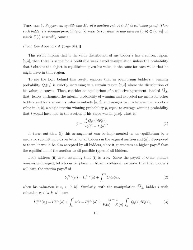
Theorem 1. Suppose an equilibrium MA of a auction rule A ∈ A∗ is collusion-proof. Then
each bidder i’s winning probability Qi(·) must be constant in any interval (a, b) ⊂ (ri, vi] on
which Fi(·) is weakly convex.
Proof. See Appendix A (page 34).
This result implies that if the value distribution of say bidder i has a convex region,
[a, b], then there is scope for a profitable weak cartel manipulation unless the probability
that i obtains the object in equilibrium given his value, is the same for each value that he
might have in that region.
To see the logic behind this result, suppose that in equilibrium bidder’s i winning
probability Qi(vi) is strictly increasing in a certain region [a, b] where the distribution of
his values is convex. Then, consider an equilibrium of a collusive agreement, labeled MA,
that: leaves unchanged the interim probability of winning and expected payments for other
bidders and for i when his value is outside [a, b]; and assigns to i, whenever he reports a
value in [a, b], a single interim winning probability p, equal to average winning probability
that i would have had in the auction if his value was in [a, b]. That is,
p =
∫ baQi(s)dFi(s)
Fi(b)− Fi(a). (1)
It turns out that (i) this arrangement can be implemented as an equilibrium by a
mediator submitting bids on behalf of all bidders in the original auction and (ii), if proposed
to them, it would be also accepted by all bidders, since it guarantees an higher payoff than
the equilibrium of the auction to all possible types of all bidders.
Let’s address (ii) first, assuming that (i) is true. Since the payoff of other bidders
remains unchanged, let’s focus on player i. Absent collusion, we know that that bidder i
will earn the interim payoff of
UMAi (vi) = UMA
i (a) +
∫ vi
a
Qi(s)ds, (2)
when his valuation is vi ∈ [a, b]. Similarly, with the manipulation MA, bidder i with
valuation vi ∈ [a, b] will earn
U MAi (vi) = UMA
i (a) +
∫ b
a
pds = UMAi (a) +
vi − aFi(b)− Fi(a)
∫ vi
a
Qi(s)dFi(s), (3)
13

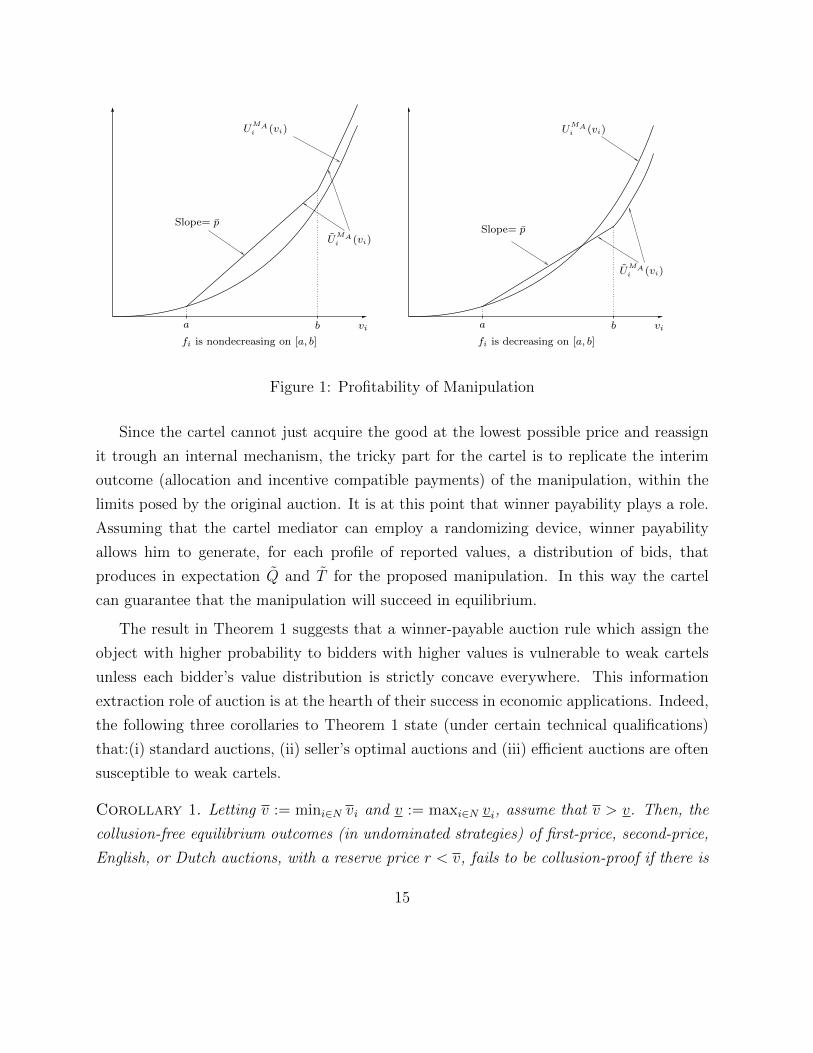
where the last equality follows from (1). Note that the payoff in both cases rises at a
speed equal to the winning probability. Since Qi rises strictly whereas p is constant, the
payoff without manipulation is strictly convex whereas the payoff under manipulation rises
linearly, as depicted by Figure 1. Essentially the manipulation speeds up the rate of payoff
increase for lower value and slows down the rate for the higher value. Since Fi is convex in
[a, b] and since Qi is strictly increasing,∫ b
a
Qi(s)dFi(s) ≥Fi(b)− Fi(a)
b− a
∫ b
a
Qi(s)ds. (4)
Substituting (4) into (3) for vi = b, we get
U MAi (b) ≥ UMA
i (a) +
∫ b
a
Qi(s)ds = UMAi (b). (5)
In other words, bidder i with valuation vi = b will be at least weakly better off from the
manipulation. Given the curvatures of these two utility functions, then the bidder will be
strictly better off from the manipulation for any intermediate value vi ∈ (a, b) (see the left
panel of Figure 1).
The same argument explains why this weak cartel manipulation may not work if the
bidder’s value distribution is strictly concave. In this latter case, the inequality of (4) is
reversed. Hence, as shown in the right panel of Figure 1, bidder with sufficiently high type
vi ≈ b will be strictly worse off from the manipulation. In other words, in this case the
weak cartel will not be able to induce high value bidders to join the collusive agreement.
Finally, to complete our argument we need to show that the proposed manipulation
of the original auction can be implemented by the cartel in a technologically feasible and
incentive compatible fashion. In fact, pooling requires shifting the winning probability
away from high types toward low value types of bidder i, and it is not clear whether and
how the shifting of the winning probabilities can be engineered to occur in equilibrium,
especially without altering the payoffs of the other bidders.
As a first step, observe that the proposed agreement could be implemented as an equi-
librium if bidders were able to design an auction themselves. In fact it can be verified that
the proposed profile of interim probabilities functions Q in MA satisfies the conditions set
forth at the end of in Section 2, that is (MN) and (B).
14
a b vi
UMAi (vi)
fi is decreasing on [a, b]
a b vi
UMAi (vi)
fi is nondecreasing on [a, b]
UMAi (vi)
UMAi (vi)
Slope= pSlope= p
Figure 1: Profitability of Manipulation
Since the cartel cannot just acquire the good at the lowest possible price and reassign
it trough an internal mechanism, the tricky part for the cartel is to replicate the interim
outcome (allocation and incentive compatible payments) of the manipulation, within the
limits posed by the original auction. It is at this point that winner payability plays a role.
Assuming that the cartel mediator can employ a randomizing device, winner payability
allows him to generate, for each profile of reported values, a distribution of bids, that
produces in expectation Q and T for the proposed manipulation. In this way the cartel
can guarantee that the manipulation will succeed in equilibrium.
The result in Theorem 1 suggests that a winner-payable auction rule which assign the
object with higher probability to bidders with higher values is vulnerable to weak cartels
unless each bidder’s value distribution is strictly concave everywhere. This information
extraction role of auction is at the hearth of their success in economic applications. Indeed,
the following three corollaries to Theorem 1 state (under certain technical qualifications)
that:(i) standard auctions, (ii) seller’s optimal auctions and (iii) efficient auctions are often
susceptible to weak cartels.
Corollary 1. Letting v := mini∈N vi and v := maxi∈N vi, assume that v > v. Then, the
collusion-free equilibrium outcomes (in undominated strategies) of first-price, second-price,
English, or Dutch auctions, with a reserve price r < v, fails to be collusion-proof if there is
15

a bidder i for whom fi is non-increasing on some interval (a, b) ⊂ Vi with b > r and a ≥ v.
Proof. See Appendix A (page 37).
Corollary 2. Assume that the virtual valuations, Ji(vi) = vi − 1−Fi(vi)fi(vi)
, are absolutely
continuous, always positive, and strictly increasing for all i ∈ N . Furthermore, assume
that there exists a player i and an interval of his value space [a, b] ∈ Vi where fi is non-
increasing such that Ji(b) > maxj 6=i Jj(vj). Then, the equilibrium outcome that maximizes
the seller’s revenues (i.e. the equilibrium of Myerson’s optimal auction) fails to be collusion
proof.
Proof. The hypotheses guarantee that there exists an interval [b− ε, b], with ε > 0, where
Qi(vi) is strictly increasing. The result then follows from Theorem 1.
Corollary 3. Suppose that there is some bidder i such that [vi, vi]∩[minj 6=i vj,maxj 6=i vj] 6=∅ and fi is nonincreasing somewhere in the interval [vi, vi] ∩ [minj 6=i vj,maxj 6=i vj]. Then,
any ex-post efficient equilibrium outcome of an auction rule is fails to be collusion-proof.
Proof. The result follows from the Theorem 1 and the observation that given the efficient
allocation, the interim winning probability of bidder i is increasing in the interval [vi, vi]∩[minj 6=i vj,maxj 6=i vj].
The next result establishes a converse of Theorem 1. Sufficiency requires that two
further conditions are added, representing minimal optimality requirements from the seller’s
perspective.
Theorem 2. Suppose an auction rule A ∈ A∗ satisfies τi(b) ≥ ξi(b)vi,∀b ∈ B,∀i and
satisfies condition (B) with equality at r1, . . . , rn. If its collusion-free equilibrium outcome
has the interim allocation Qi(·) constant wherever Fi(·) is locally convex, for each i ∈ N ,
then the chosen equilibrium outcome is collusion proof.
Proof. See Appendix A (page 38).
The two preliminary conditions rule out auctions that are clearly inefficient from the
seller’s perspective, in the sense that do not exploit all allocation capacity available to
16

the seller above the reserve price, and that sell the good to a bidder at a price below his
lowest possible value.12 Once these technical conditions are taken into account, the intuition
behind this result is essentially the same as for Theorem 1. In other words, starting from the
suggested equilibrium, any manipulation including, but not limited to, those that involve
pooling of some types, must leave some bidder types strictly worse off. This explains that
successful collusion will be very difficult to mount on the part of bidders.
Theorem 2 has the following immediate corollary, which collects in a single statement
the natural counterparts to the three previous corollaries to Theorem 1.
Corollary 4. If fi is strictly decreasing for all i ∈ N , then the following equilibria
are collusion proof: (i) the collusion-free equilibrium equilibria of first-price, second-price,
English, or Dutch auctions, with a reserve price r ≥ maxi∈N vi (ii) any equilibrium of any
auction τi(b) ≥ ξi(b)vi,∀b ∈ B,∀i that results in an a efficient allocation, and (iii) any
equilibrium of any auction that maximizes the seller’s revenue.
Proof. The proof is immediate given Theorem 2 and the fact that fi is strictly decreasing
for all i ∈ N .
We conclude this section by outlining a more precise comparison of our result with those
of MM. Recall from MM that if symmetric bidders make an ex-ante decision to participate
in a cartel, the first-price auction is susceptible (unsusceptible) to weak cartel if the inverse
hazard rate 1−F (·)f(·) is decreasing (increasing) and that, if it is increasing, the only collusion-
proof mechanism is a completely random allocation rule. First of all, in contrast to MM we
consider asymmetric bidders and distribution with non-monotonic hazard rate. However,
even if we maintain the monotonic inverse hazard rate assumption, their condition for
auctions to be susceptible to weak cartels does not coincide with ours. In particular, note
that a nondecreasing density f(·) is sufficient, but not necessary, for the inverse hazard rate
12It is easy to see that without a reserve price high enough when the lowest possible valuation is sufficiently
high, all standard auctions are susceptible to weak cartels. Consider, for instance, a first-price auction in
which the lower bound of value support, v, is very high while there is no reserve price. Then, bidders will
find it Pareto-improving to identically bid zero and share the object with equal probability.
17
to be decreasing.13 Thus, according to Corollary 1 and 4, standard auctions are susceptible
to weak cartel in MM’s sense whenever it is so in our sense, but the converse does not hold.
In this sense our definition is weaker. The distinction arises from whether the incentives
for participating to a cartel is ex ante or interim. Since interim incentives for participation
are more difficult to satisfy then ex ante incentives, MM’s theory tends to overstate the
susceptibility of auctions to collusion.
4 Optimal Collusion-Proof Auctions
For many typical distributions the corresponding density is not nondecreasing in the entire
support. In these cases, requiring collusion-proofness need not prescribe a completely
random allocation of the good. This suggests that in most cases there is a scope for
designing a reasonably well-performing auction rule that is collusion proof. In this section,
we take up this issue and look for the the auction that maximizes the seller’s revenue among
all collusion-proof auctions.
To obtain an optimal collusion proof auction we make use of the characterization re-
sults from the previous section, especially the necessary condition given in the Theorem 1.
Without loss of generality, we proceed by restricting attention to incentive compatible di-
rect revelation mechanisms. Once an optimal direct mechanism is found, a corresponding
winner payable auction can always be obtained.
Recall that Ji(v) = v − 1−Fi(v)fi(v)
is the virtual valuation function for player i. Using
the characterization of implementable outcomes provided in section 2 we can write our
maximization problem as follows:
[P ] max(Qi(·),Ti(vi))ni=1
∑i∈N
∫ vi
ri
Ji(s)Qi(s)dFi(s)−∑i∈N
[Qi(vi)vi − Ti(vi)],
13To see it, note
d
dv
(1− F (v)
f(v)
)=−f(v)2 − f ′(v)(1− F (v))
f(v)2< 0 if f ′(v) ≥ 0.
18

subject to (B), (MN), (IR) and the collusion-proof constraint:
Qi(·) is constant where fi(·) is nondecreasing,∀i ∈ N. (6)
The objective function is the (well-known) expression of the seller’s expected revenue
that derives from using the incentive compatibility condition (TR) to substitute the al-
location rule for the payment rule. The constraints (MN) and (IR) are required for the
incentive compatibility and individual rationality, respectively. Lastly, the constraint (6)
corresponds to the necessary condition for the weak collusion-proofness drawn from the
Theorem 1. Henceforth assume that T (vi) = viQi(vi) since this is the best that the auc-
tioneer can do subject to (IR) being always satisfied.
Unfortunately, the program [P ] is not subject to our analysis in its full generality. In
order to obtain an analytical solution we need to focus on the class of symmetric distribu-
tions whose density is single-peaked. That is we assume that for each i ∈ N , Fi(·) = F (·)for some F (·) and there is a value v∗ ∈ V = [v, v] such that the density f(v) is continuously
increasing if v < v∗ and decreasing otherwise. Furthermore, we restrict attention to the so
called regular case and therefore assume that the virtual valuation J(v) is non-decreasing.
There are many distributions belonging to this class, including Cauchy, Exponential, Lo-
gistic, Normal, Uniform, Weibull, and others. Our analysis extends later on to the case of
asymmetric bidders if fi is either increasing or decreasing over the entire range Vi for all
i ∈ N .
First, let v = maxJ−1(0), v. When v∗ ≤ v, then the density is strictly decreasing.
In this case we already know that, according to Corollary 4 (iii), the Myerson’s optimal
auction is collusion proof. Therefore, henceforth assume that v∗ > v. To make our main
result more transparent, we derive it in four lemmas.
Lemma 2. At the optimum of [P ], it must be that v∗ > ri ≥ v for all i ∈ N
Proof. Refer to the Appendix B (page 40).
Recalling the definition of ri (i.e. supv : Qi(v) = 0), and the fact that the virtual
valuation function is increasing, the lemma states that at the optimum bidders who have
negative virtual value must have a zero probability of obtaining the object in equilibrium.
19

This property is shared with the optimal mechanism when collusion is not present. Fur-
thermore the lemma provides an upper bound, equal to v∗, to set of values that can be
assigned zero probability at the optimum.
Collusion proofness requires that Qi(·) is constant in the interval [ri, v∗). Therefore,
define pi = Qi(v) for v ∈ [ri, v∗). Note that we can then rewrite the objective as:
maxmax(Qi(·),pi,ri)ni=1
∑i∈N
pi ·∫ v∗
ri
J(v)f(v)dv +∑i∈N
∫ v
v∗J(v)Qi(v)f(v)dv
Ignore for a moment the monotonicity constraint (MN), which will turn out to be satis-
fied at the optimum. Since the collusion proof constraint (6) constraint is now embedded in
the objective, the only constraint that the auctioneer needs to take care of is the feasibility
constraint (B). In particular, under this constraint the designer faces a trade-off between
assigning more often the object to low values and high value bidders. The next Lemma
shows that since since J(·) is increasing, at the optimum of [P ] the seller will want to shift
as much probability as possible toward high value bidders. Therefore the constraint (B)
will be binding at (at least) at all profiles (v, . . . , v) for each v > v∗.
Lemma 3. At the optimum of [P ], it must be that∑
i∈N∫ vvQi(s)f(s)ds = 1 − F (v)n for
all v ∈ [v∗, v]
Proof. Refer to the Appendix B (page 20).
It turns out that the condition in the above Lemma uniquely identify a profile of alloca-
tion rules for the interval [v∗, v]. In particular, the interim allocation rule restricted to the
interval [v∗, v] must be the one arising from an efficient allocation of the object. In fact, the
only way to assign to each interval to the left of the highest valuation, for each player, an
average probability of getting the object equal to the probability that he has value above
the lower bound of the interval is to assign always the good to the player with the highest
valuation.
Lemma 4. Suppose that∑
i∈N∫ vvQi(s)f(s)ds = 1 − F (v)n,∀v ∈ [v∗, v]. Then, the only
interim allocation rule that satisfies (B) and (MN) is
Qi(v) = F (v)n−1,∀v ∈ (v∗, v],∀i ∈ N. (7)
20
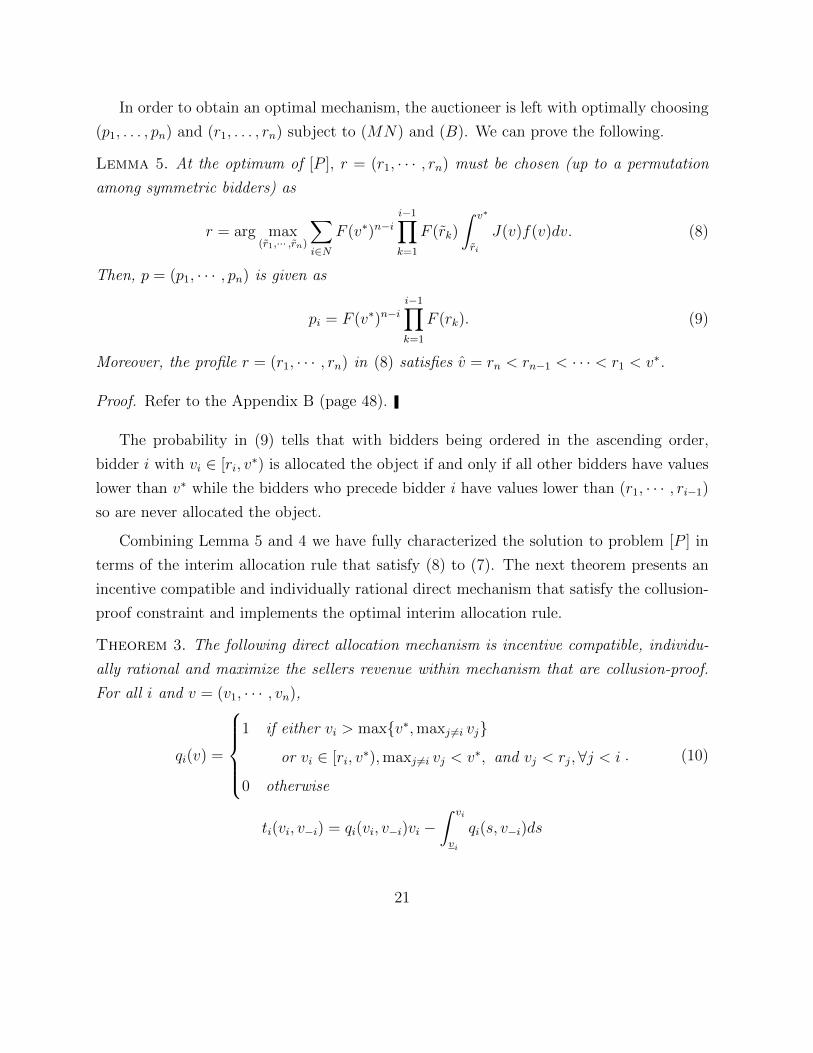
In order to obtain an optimal mechanism, the auctioneer is left with optimally choosing
(p1, . . . , pn) and (r1, . . . , rn) subject to (MN) and (B). We can prove the following.
Lemma 5. At the optimum of [P ], r = (r1, · · · , rn) must be chosen (up to a permutation
among symmetric bidders) as
r = arg max(r1,··· ,rn)
∑i∈N
F (v∗)n−ii−1∏k=1
F (rk)
∫ v∗
ri
J(v)f(v)dv. (8)
Then, p = (p1, · · · , pn) is given as
pi = F (v∗)n−ii−1∏k=1
F (rk). (9)
Moreover, the profile r = (r1, · · · , rn) in (8) satisfies v = rn < rn−1 < · · · < r1 < v∗.
Proof. Refer to the Appendix B (page 48).
The probability in (9) tells that with bidders being ordered in the ascending order,
bidder i with vi ∈ [ri, v∗) is allocated the object if and only if all other bidders have values
lower than v∗ while the bidders who precede bidder i have values lower than (r1, · · · , ri−1)
so are never allocated the object.
Combining Lemma 5 and 4 we have fully characterized the solution to problem [P ] in
terms of the interim allocation rule that satisfy (8) to (7). The next theorem presents an
incentive compatible and individually rational direct mechanism that satisfy the collusion-
proof constraint and implements the optimal interim allocation rule.
Theorem 3. The following direct allocation mechanism is incentive compatible, individu-
ally rational and maximize the sellers revenue within mechanism that are collusion-proof.
For all i and v = (v1, · · · , vn),
qi(v) =
1 if either vi > maxv∗,maxj 6=i vj
or vi ∈ [ri, v∗),maxj 6=i vj < v∗, and vj < rj,∀j < i
0 otherwise
. (10)
ti(vi, v−i) = qi(vi, v−i)vi −∫ vi
vi
qi(s, v−i)ds
21

Proof. By Lemma 3 and 5, the allocation (Q, p, r) given in (7) to (8) solves [P ]. It suffices to
check that the ex-post allocation rule in (10) generates (Q, p, r), which is straightforward.
The allocation in (10) can be interpreted as the procedure where the seller first tries to
sell the object to an efficient bidder if there is some bidder with value above v∗. If all bidders
have values falling short of v∗, then the seller turns to sequentially approach bidders in the
ascending order and sell the object to whomever first claims that his value is no lower than
his reserve price. This direct mechanism can be implemented by a simple winner-payable
auction rule combining the second-price auction and sequential take-it-or-leave offers, as
seen in the following result:
Corollary 5. Consider ri and pi defined in (8) and (9), and define Ri to satisfy
(v∗ −Ri)F (v∗)n−1 = (v∗ − ri)pi. (11)
Then, the solution of the program [P ] can be implemented via the equilibrium of a second-
price (or English) auction with the individualized minimum price Ri for each bidder i that
is followed by the sequential take-it-or-leave offers with ri being offered to bidder i.
Proof. The left and right hand sides of (11) correspond to the payoffs that bidder i with
value v∗ can obtain in the second-price auction and in the sequential take-it-or leave offers,
respectively, provided that all other bidder j bids his value in the second-price auction if
vj ≥ v∗ while bidding zero to accept the offer rj afterwards if vj ∈ [rj, v∗). Since bidder
i with value v∗ is indifferent between two payoffs, it is straightforward to see that absent
collusion, the optimal strategy for bidder i is also to bid his value in the second-price
auction if vi ≥ v∗, and to bid zero and accept the offer ri afterwards if vi ∈ [ri, v∗). Clearly,
this auction rule and its equilibrium outcome satisfy the requirement in the Theorem 2 and
thus is collusion-proof.
An interesting feature of our optimal auction rule is that it treats bidders asymmet-
rically though they are ex-ante symmetric. This feature arises because the seller cannot
perform screening of values in a certain interval of the value space due to the collusion-proof
constraint, but finds profitable to implement a partial screening by discriminating values
across ex-ante identical bidders instead. In this light, the asymmetric mechanisms can be
a useful device to increase revenues against collusive bidders.
22

However, the mechanisms that treat the ex-ante symmetric bidders asymmetrically
might not be allowed for some exogenous reason such as the fairness consideration. The
following result provides the optimal allocation rule under the restriction that the auction
rule has to be symmetric.
Proposition 1. An optimal symmetric collusion-proof auction rule has the interim allo-
cation rule Qs(·) such that
Qs(v) =
F (v)n−1 if v ≥ v∗
ps if v ∈ [rs, v∗)
0 otherwise
,
where
rs = arg maxr∈[v,v∗]
( n∑i=1
F (v∗)n−iF (r)i−1)∫ v∗
r
J(s)f(s)ds
and
ps :=F (v∗)n − F (rs)
n
n[F (v∗)− F (rs)]=
∑ni=1 F (v∗)n−iF (rs)
i−1
n.
This interim allocation can be implemented by the following ex-post incentive compatible
direct mechanism: For all i and v = (v1, · · · , vn),
qi(v) =
1 if vi > maxv∗,maxj 6=i vj
1#j∈N | vj∈[rs,v∗) if vi ∈ [rs, v
∗) and maxj 6=i vj < v∗
0 otherwise
. (12)
ti(vi, v−i) = qi(vi, v−i)vi −∫ vi
vi
qi(s, v−i)ds
Proof. Refer to the Appendix B (page 50).
The common reserve price rs is chosen to maximize the seller’s revenue in the posted-
price sale that arises when he fails to sell the object to the types above v∗. As in the
Corollary 5, this allocation rule can also be implemented via the second-price auction with
23

an appropriate, symmetric, minimum price that is followed by the sale at the posted-price
rs.14
Before closing this section, we discuss the case of asymmetric bidders in which the
density fi is decreasing or nondecreasing for all i ∈ N . In case all fi’s are decreasing,
we have seen that Corollary 4 shows that the non-collusive optimal auction is collusion-
proof, implying that the collusion entails no loss for the seller. Turning to the case of
nondecreasing fi’s, Theorem 1 requires the interim winning probability for each bidder i
to be constant at some pi in the range [ri, vi] and to be equal to zero in [vi, ri). Thus, the
seller’s problem is
max(ri)i∈N
∑i∈N
pi
∫ vi
ri
Ji(s)fi(s)ds =∑i∈N
pi(1− Fi(ri))ri (13)
subject to p = (p1, · · · , pn) satisfying (B). The following result characterize the solution of
this problem.
Proposition 2. Suppose that all fi’s are nondecreasing. Then, the seller’s problem amounts
to solving
maxπ∈Π
[max
(ri)i∈N
∑i∈N
( ∏j:π(j)<π(i)
Fj(rj))
(1− Fi(ri)) ri], (14)
where Π the set of all permutation functions π : N → N .
Proof. Refer to the Appendix B (page 51).
Here π represents the order according to which the seller makes the sequential take-it-or-
leave offers (r1, · · · , rn). Given an order π, each bidder i will receive the seller’s offer if all
bidders before him turn down, which occurs with probability∏
j:π(j)<π(i) Fj(rj). The term in
the square bracket of (14) corresponds to the expected revenue from the sequential take-it-
or-leave-it offers optimally chosen under the given order π. Once the revenue is maximized
14Speaking precisely, the minimum price R has to be at such level that v∗ is indifferent between bidding
v∗ in the auction and paying rs in the posted price sale, namely
(v∗ −R)F (v∗)n−1 = (v∗ − rs)ps.
24

under each possible order, the seller chooses the order that achieves the highest revenue,
which is what the maximization problem outside the square bracket does. Obviously, when
agents are ex-ante identical the order will not matter.
5 Strengthening the Notion of Collusion-Proofness
The notion of collusion-proofness that we outlined assumes that a cartel will form if and
only if it can benefit all the bidders for sure, compared to the payoff that they would obtain
by playing the equilibrium of the auction. Our definition is weaker than that set forth in
MM, whereby a cartel will form whenever it makes all player better off in expectation.
However, it is still somewhat restrictive, since one can think at the possibility that a cartel
forms that benefits only some of the players, only some of the time. How this would come
about can be modeled by modifying the cartel formation game that we envisaged in section
2.3. We said there that whenever some cartel member decided whether or not to join the
cartel, he would do so conjecturing that the others would infer nothing in case of refusal
and that his refusal would hamper any further dialogue within the rest of the bidders,
which for this reason would not agree on forming a different cartel. Instead, one might give
the cartel a better chance if one assumes that a defector has reasons to believe that indeed
the other bidders will be able to infer his value and be also able to coordinate and punish
him. This consideration motivates the notion of robust collusion proofness, which we now
present in more details.
In what follows, we limit our discussion to truthful and individually rational equilibria
of direct auction mechanisms. Let the truthful equilibrium of one such mechanism be
MD = (q, t). We want to define a lower bound to the payoff that each bidder can expect
to get in an equilibrium of the continuation game ensuing if he does not join any cartel.
First, fix any bidder i ∈ N with valuation vi and assume that i has rejected a collusive
proposal. Consider a partition πi = C1, ..., Ck of N \i. Let Πi be the set of all possible
partitions of N \ i. Each Ci indicates a group of bidders forming a cartel and a singleton
element will mean a bidder who is not part of a cartel. We assume that bidder i assesses
that any partition of weak cartels may be active in the continuation equilibrium.
Furthermore, we assume that bidder i conjectures that all the other bidders will infer
25

his type precisely (the worst possible case for him) and punish him in a coordinated way
by playing cartel undominated strategies. We define the latter concept as follows. For any
subset C ⊂ N , let vC = (vi)i∈C and vN\C = (vi)i 6∈C(v) be the profiles of values within the
set and outside that set. Let uMi (v|vi) = viqi(v)− ti(v). We say a profile v′C of strategies is
dominated in MD if there is another profile v′′C such that for all i ∈ C and vN\C :
uMi (v′C , vN\C |vi) ≤ uMi (v′′C , vN\C |vi)
Let Ω(vC) ⊂∏
i∈C Vi be the set of undominated strategies for type profile vC , i.e.,
strategies that do not satisfy the above condition. Then, the lower bound can be described
as
UM
(vi) := supv′i∈Vi
Ev−i[
infuMi (v′i, v
′C1 , ..., v′Ck |vi)
∣∣∣v′Cj ∈ Ω(vCj), Cj ∈ πi, πi ∈ Πi
].
This lower bound is the expected payoff for bidder i in the worst-case-scenario where, in
case he defects, the other bidders precisely infer his type and form a partition of weak
cartels and choose undominated strategy profiles as to minimize his payoff.
We can now state our definition of robust collusion proofness. We presume that each
bidder will be willing to join the cartel if it promises him no less payoff than the that lower
bound, which will have the effect of making it easier for cartels to form and more difficult
for the seller to fight against it. As before, MD represents a manipulation of the original
auction by weak cartels, though if acceptance is not unanimous the continuation is different
from the default auction outcome.
Definition 3. A direct auction mechanism M is robustly collusion-proof if there exists no
weak cartel manipulation MA of A satisfying (IC) and
(R− CIRMA) U M
i (vi) ≥ UM
i (vi), ∀vi, i, with strict inequality for some vi, i.
It is important to note that we are now able to manage the possibility that only a
group of bidders is actively engaged in a collusive agreement, provided that they never
employ dominated strategies and other bidders can rationally expect this. In fact, it is
without loss of generality to assume that the cartel is all inclusive (i.e. that all bidders are
offered to participate and that all types will accept the offer). Consider any equilibrium
26

where the cartel only consists in a subset of bidders, some types possibly reject the offer,
and everyone plays undominated strategies. Then there is a payoff-equivalent equilibrium
where all bidders join a cartel, designed in a such a way that everyone is requested to make
the same report in the mechanism that he would have made in the other equilibrium, or
in case he refused to join. Finally, note that the assumption of rational expectation for
non-cartel bidders is unnecessary if the original mechanism is dominant strategy incentive
compatible (DSIC).15 In this case, non-cartel bidders need not know about what cartels
are existing or who is in what cartel.
Next, we define a property of incentive compatible direct mechanisms, which we call
monotone dominant strategy incentive compatibility (mDSIC) and we show that it is suffi-
cient to guarantee that whenever an equilibrium of an auction is collusion proof, then it is
also robustly collusion proof. Therefore any outcome that is collusion proof, including the
optimal collusion proof auction, can be robustly collusion proof implemented.
Definition 4. A direct auction mechanism (q, t) is monotonic DSIC (or mDSIC) if qi is
nondecreasing in vi and nonincreasing in v−i, and
ti(vi, v−i) = qi(vi, v−i)vi −∫ vi
vi
qi(s, v−i)ds. (15)
Note that this property is slightly stronger than the usual DSIC property since it requires
qi to be nonincreasing with v−i. As anticipated, the following establishes the sufficiency of
the mDSIC property for an auction that is collusion proof to be also robustly so.
Theorem 4. If an direct auction mechanism MD := (q, t) is mDSIC and collusion-proof,
then it is robustly collusion-proof.
Proof. Fix a bidder i with any value vi. If he reports truthfully, and others report any
arbitrary v−i, then he earns
uMi (vi, v−i|vi) = viqi(vi, v−i)− ti(vi, v−i) =
∫ vi
vi
qi(s, v−i)ds.
Since qi is decreasing in v−i, his payoff is decreasing in v−i.
15The obvious reason is that they can simply use their dominant strategies regardless of what cartels do.
27

Now fix any coalition C of bidders and their types vC . Consider any strategy profile of
that coalition v′C . Suppose that v′i > vi for some i ∈ C. Then,∑j∈C
uMj (v′C , vN\C |vj) ≤∑j∈C
uMj (vi, v′C\i, vN\C |vj),∀vN\C , (16)
since dominant strategy incentive compatibility M for bidder i means that
uMi (v′C , vN\C |vi) ≤ uMi (vi, v′C\i, vN\C |vi),∀vN\C ,
and since, for j ∈ C \ i, vi < v′i implies that:
uMj (v′C , vN\C |vj) ≤ uMj (vi, v′C\i, vN\C |vj),∀vN\C .
[Need to change the definition of dominance with respect to strict inequalities vs. weak
inequalities.]Then, (16) implies that if v′C ∈ Ω(vC), then we must have v′C ≤ vC (in weak
vector inequalities).
Then, for each possible profile v−i of the remaining bidders and for any arbitrary πi =
C1, ..., Ck ∈ Πi. if v′Cj ∈ Ω(vCj), then v′Cj ≤ vCj , so we have
uMi (vi, v′C1 , ..., v′Ck |vi) ≥ uMi (vi, v−i|vi).
It thus follows that
UM
i (vi) ≥ Ev−i [uMi (vi, v−i|vi)] = UMi (vi). (17)
Let us now suppose for a contradiction that M is not robustly WC collusion-proof, which
means there exists a manipulation M satisfying (IC) and (R−CIRMA). Combining (R−
CIRMA) and (17), we have M interim Pareto dominating the auction, which contradicts
the collusion-proofness of M .
Since it turns out that the optimal collusion-proof auctions we characterized in the
previous section has an mDSIC allocation rule, we can conclude that it is also robustly
collusion-proof.
Corollary 6. The optimal allocation rules described in Theorem 3 and Proposition 1 can
be implemented via a robustly collusion-proof auction mechanism.
Proof. It suffices to check that the ex-post allocation rules in (10) and (12) are mDSIC,
which is straightforward.
28

Appendix A: Proof of Lemma 1
Since the revelation principle shows that any equilibrium of any auction can be achieved
as an equilibrium of an incentive compatible direct mechanism, we only need to show two
things. First, we show that any outcome of an incentive compatible direct mechanism
can be achieved as an equilibrium of a winner payable auction. Second, following Border
(1991,2007) we will show that that there exists an incentive compatible direct mechanism
that induces interim winning probability as in Q if and only if Q satisfies (MN) and (B)
The first point is easy to prove. Take an incentive compatible direct mechanism ex-post
allocation rule and use the following payment rule:
ti(vi, v−i) = qi(vi, v−i)vi −∫ vi
vi
qi(s, v−i)ds,
modifying it to require that, in case of randomization, only the winner of the object wins.
It is well known that the auction rule constructed in this way will satisfy (LW ) and (TR)
if Q satisfies (MN). Then, modify the direct mechanism by adding a set of profile of
reports that make the auction winner payable. Do so in a way that does not eliminate the
original equilibrium of the mechanism. One can do this, for example, by adding, for each
possible payment and bidder, a profile of signals (one for each bidder) which makes that
bidder pay that payment and win the object, while everyone else gets nothing. The original
equilibrium is not altered since these added profiles are never played in equilibrium and do
not represent, individually, a profitable deviation.
Our proof for the second statement is an extension of the proofs in Border (1991,2007)
to the case of asymmetric bidders and continuous distributions. Without loss of generality,
we restrict attention to direct revelation mechanisms. The fact that doing so is without
loss is clear for the if part: if we find a direct mechanism, we have found an auction. The
only if part follows from the revelation principle. We say that Q is implementable if there
exists a direct revelation mechanisms that implements it.
We let λi denote the probability measure associated with the distribution Fi. We first
prove the result when there are finite types and extend it to the case of continuum of types.
29

Finite Type Case Each bidder i ∈ N independently draws his value vi from the support
Vi = vi1, vi2, · · · , vimi following a probability measure λi. With function Qi : Vi → [0, 1]
denoting bidder i’s interim winning probability, we assume that16
Qi(vi1) ≥ · · · ≥ Qi(vimi), ∀i ∈ N. (18)
Given any set A =∏
i∈N Ai ⊂ V , let
B(A) := 1−∏i∈N
(1− λi(Ai)),
that is the probability that at least one bidder i draws his value from Ai. Then, Border
(2007) proves the following result:17
Result 1. A profile of interim winning probabilities Q1, · · · , Qn is implementable if and
only if ∑i∈N
∑vi∈Ai
Qi(vi)λi(vi) ≤ B(A),∀A =∏i∈N
Ai ⊂ V . (19)
Proof. See Border (2007).
Border’s condition is not very convenient for applications since it has to be checked
for all subsets of types. Hence, we relax this condition to require (19) to be satisfied
for hierarchical sets only: Letting Eik := vi1, · · · , vik for each i and k, define E :=
∏
i∈N Eiki ⊂ V | ki = 1, · · · ,mi,∀i ∈ N. The following Result extends Lemma 5.5 of
Border (1991) to the case of asymmetric bidders.
Result 2. Consider any profile of interim winning probabilities Q1, · · · , Qn satisfying (18).
Then, (19) holds if and only if it holds for any profile of hierarchical subsets∏
i∈N Eiki ∈ E,
that is ∑i∈N
∑j≤ki
Qi(vij)λi(vij) ≤ B(∏i∈N
Eiki
),∀k1, · · · , kn. (20)
16Note that Qi need not be increasing in value since values vi1, · · · , vimiare not necessarily ordered
according to their magnitude.17In fact, Border (2007) proves this result by allowing for correlated types.
30
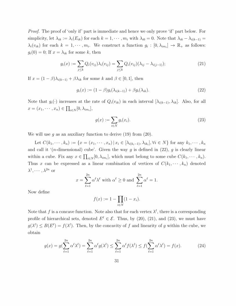
Proof. The proof of ‘only if’ part is immediate and hence we only prove ‘if’ part below. For
simplicity, let λik := λi(Eik) for each k = 1, · · · ,mi with λi0 = 0. Note that λik − λi(k−1) =
λi(vik) for each k = 1, · · · ,mi. We construct a function gi : [0, λimi ] → R+ as follows:
gi(0) = 0; If x = λik for some k, then
gi(x) :=∑j≤k
Qi(vij)λi(vij) =∑j≤k
Qi(vij)(λij − λi(j−1)); (21)
If x = (1− β)λi(k−1) + βλik for some k and β ∈ [0, 1], then
gi(x) := (1− β)gi(λi(k−1)) + βgi(λik). (22)
Note that gi(·) increases at the rate of Qi(vik) in each interval [λi(k−1), λik]. Also, for all
x = (x1, · · · , xn) ∈∏
i∈N [0, λimi ],
g(x) :=∑i∈N
gi(xi). (23)
We will use g as an auxiliary function to derive (19) from (20).
Let C(k1, · · · , kn) := x = (x1, · · · , xn) |xi ∈ [λi(ki−1), λiki ],∀i ∈ N for any k1, · · · , knand call it ‘(n-dimensional) cube’. Given the way g is defined in (22), g is clearly linear
within a cube. Fix any x ∈∏
i∈N [0, λimi ], which must belong to some cube C(k1, · · · , kn).
Thus x can be expressed as a linear combination of vertices of C(k1, · · · , kn) denoted
λ1, · · · , λ2n or
x =2n∑`=1
α`λ` with α` ≥ 0 and2n∑`=1
α` = 1.
Now define
f(x) := 1−∏i∈N
(1− xi).
Note that f is a concave function. Note also that for each vertex λ`, there is a corresponding
profile of hierarchical sets, denoted E` ∈ E . Thus, by (20), (21), and (23), we must have
g(λ`) ≤ B(E`) = f(λ`). Then, by the concavity of f and linearity of g within the cube, we
obtain
g(x) = g(2n∑`=1
α`λ`) =2n∑`=1
α`g(λ`) ≤2n∑`=1
α`f(λ`) ≤ f(2n∑`=1
α`λ`) = f(x). (24)
31

To show (19), pick any set A = (A1, · · · , An) ⊂ V . Letting λik := λi(Eik ∩ Ai) and
λi0 = 0, we construct another function hi : [0, λimi ] → R+ analogously to gi: hi(0) = 0; If
x = λik for some k, then
hi(x) :=∑j≤k
Qi(vij)λi(vij ∩ Ai) =∑j≤k
Qi(vij)(λij − λi(j−1));
If x = (1− β)λi(k−1) + βλik for some k and β ∈ [0, 1], then
hi(x) := (1− β)hi(λi(k−1)) + βhi(λik).
Also, for all x = (x1, · · · , xn) ∈∏
i∈N [0, λimi ],
h(x) :=∑i∈N
hi(xi).
We show hi(x) ≤ gi(x),∀x ∈ [0, λimi ]. Note first that λik − λi(k−1) ≤ λik − λi(k−1) for all
k = 1, · · · ,mi. Thus, if x ∈ [λi(k−1), λik] for some k, then we must have x ∈ [λi(k′−1), λik′ ] for
some k′ ≤ k, which implies that when hi(·) increases at the rate of Qi(vik), gi(·) increases
at the rate of Qi(vik′) ≥ Qi(vik). This implies gi(x) ≥ hi(x) for all x ∈ [0, λimi ] given
gi(0) = hi(0) = 0.
Given the arguments above, it is straightforward that h(x) ≤ g(x) ≤ f(x) for all
x ∈∏
i∈N [0, λimi ]. To conclude, note that Eimi ∩ Ai = Ai and thus λimi = λi(Ai), which
implies∑vi∈Ai
Qi(vi)λi(vi) =∑j≤mi
Qi(vij)λi(vij ∩ Ai) = hi(λimi) = hi(λi(Ai)) ≤ gi(λi(Ai)).
This in turn implies∑i∈N
∑vi∈Ai
Qi(vi)λi(vi) = h(λ1(A1), · · · , λn(An))
≤ g(λ1(A1), · · · , λn(An))
≤ f(λ1(A1), · · · , λn(An)) = B(A)
as desired.
Result 3. A profile of interim winning probabilities Q1, · · · , Qn is implementable if and
only if (20) holds.
32

Continuum Type Case Suppose now that Vi ⊂ R is any compact space with (non-
atomic) probability measure λi. Let vi and vi denote the upper and lower bounds of Vi.Given any (nondecreasing) interim probability Qi : Vi → [0, 1] for each i ∈ N , we rewrite
the condition (B) here
∑i∈N
∫ vi
vi
Qi(ti)dλi(ti) ≤ B(∏i∈N
[vi, vi])
= 1−∏i∈N
(1− λi([vi, vi])),∀(v1, · · · , vn) ∈ V . (25)
Result 4 (Necessity). The condition (25) is necessary for Q to be implementable.
Proof. The result immediately follows from noting that∑i∈N
∫ vi
vi
Qi(ti)dλi(ti) = E[∑i∈N
qi(t) · 1t∈[vi,vi]×V−i
]≤ E
[(∑i∈N
qi(t))· 1t∈∪i∈N [vi,vi]×V−i
]≤ E
[1t∈∪i∈N [vi,vi]×V−i
]= 1−
∏i∈N
(1− λi([vi, vi])).
To prove sufficiency, we borrow the argument of Border (1991). To do so, define
D := Q = (Q1, · · · , Qn) |Q is implementable. (26)
Treat D as a subset of LN∞ =∏
i∈N L∞(λi), the (product) set of (λ1, · · · , λn)-essentially
bounded measurable functions on V . Topologize LN∞ with its weak∗, or σ(LN∞, LN1 ) topology.
Border (1991) defines D for symmetric interim probabilities and proves in the Lemma 5.4
that D is σ(L∞, L1)-compact. Since the proof easily goes through to the asymmetric case
(and is thus omitted), we can see that the set D defined in (26) is σ(LN∞, LN1 )-compact. (In
fact, the proof here can be made easier than in Border (1991) since we do not require the
auction rule implementing Q to be symmetric.)
Following Border (1991), we now approximate any asymmetric interim probabilities Q
from below by step functions: For s = 1, 2, · · · , define Qsi : Vi → [0, 1] for each i ∈ N
by setting Qsi (vi) = (2s − j)/2s if vi ∈ Vi,j/2s := ti ∈ Vi | (2s − j − 1)/2s < Qi(ti) ≤
(2s − j)/2s, j = 0, · · · , 2s. One can consider as if the set Vi,j/2s is a single type (denoted
vij), and assign it the probability equal to λi(Vi,j/2s) =: λsi (vij). Since this is equivalent to a
33

finite type case and each Qsi (vij) = (2s − j)/2s is decreasing in j, Corollary 3 is applicable,
implying that Qs = (Qs1, · · · , Qs
n) is implementable if (20) holds for Qs and λs. To verify
(20), let Eik = vi1, · · · , vik as before and then λsi (Eik) = λi(∪j≤kVi,j/2s). Letting vi,k/2s
denote the lower bound of Vi,k/2s , we obtain as desired
∑i∈N
∑j≤ki
Qsi (vij)λ
si (vij) ≤
∑i∈N
∫ vi
vi,ki/2s
Qi(ti)dλi(ti)
≤ 1−∏i∈N
(1− λi([vi,ki/2s , vi]))
= 1−∏i∈N
(1− λi(∪j≤kiVi,j/2s))
= 1−∏i∈N
(1− λsi (Eiki)),
where the first inequality follows from the fact that Qsi (vi) ≤ Qi(vi),∀vi,∀i and the second
from (25). As Border (1991) did in Proposition 3.2, we conclude that by the Lebesgue
dominated convergence theorem, Qs converges in the σ(LN∞, LN1 ) topology to Q and thus
Q is implementable since D is σ(LN∞, LN1 )-closed and each Qs belongs to D by the above
argument.
Appendix B: Proofs for Section 3
Proof of Theorem 1: Suppose for a contradiction that MA = (q, t) is collusion-proof
but Qk(·) is not constant in an interval (a,b) ⊂ (rk, vk] for some k ∈ N . Without loss of
generality consider an a > rk.
Let us define Q(·) = (Q1, · · · , Qn) as follows:
Qi(vi) =
p if i = k and vi ∈ (a, b)
Qi(vi) otherwise, (27)
where p is defined to satisfy
p(Fk(b)− Fk(a)) =
∫ b
a
Qk(s)dFk(s). (28)
34

First, note then Q satisfies (MN). At this purpose, we only need to check that:
Q(a) ≤∫ baQk(s)dFk(s)
(Fk(b)− Fk(a))≤ Q(b). (29)
The condition above holds since since F (·) is convex in (a, b). The next claim shows that,
in addition to (MN), Q also satisfies (B):
Claim 1. The interim allocation rule Q(·) satisfies (B).
Proof. Since Q(·) satisfies (B), it suffices to show that for all v ∈∏
i∈N [vi, vi],∑i∈N
∫ vi
vi
Qi(s)dFi(s) ≤∑i∈N
∫ vi
vi
Qi(s)dFi(s),
which, given (27), will hold if for all vk ∈ [vk, vk],∫ vk
vk
Qk(s)dFk(s) ≤∫ vk
vk
Qk(s)dFk(s). (30)
Note that (30) clearly holds for vk ≥ b since Qk(s) = Qk(s),∀s ∈ [b, vk]. Let us pick
vk ∈ [a, b) and then we obtain as desired∫ vk
vk
Qk(s)dFk(s) =
∫ b
vk
pdFk(s) +
∫ vk
b
Qk(s)dFk(s)
=
[Fk(b)− Fk(vk)Fk(b)− Fk(a)
] ∫ b
a
Qk(s)dFk(s) +
∫ vk
b
Qk(s)dFk(s)
≤∫ b
vk
Qk(s)dFk(s) +
∫ vk
b
Qk(s)dFk(s) =
∫ vk
vk
Qk(s)dFk(s), (31)
where the second equality follows from the definition of p, and the inequality from the fact
that Qk(·) is nondecreasing and thus∫ b
a
Qk(s)
Fk(b)− Fk(a)dFk(s) ≤
∫ b
vk
Qk(s)
Fk(b)− Fk(vk)dFk(s).
Also, for vk < a, we have∫ vk
vk
Qk(s)dFk(s) =
∫ a
vk
Qk(s)dFk(s) +
∫ vk
a
Qk(s)dFk(s)
≤∫ a
vk
Qk(s)dFk(s) +
∫ vk
a
Qk(s)dFk(s) =
∫ vk
vk
Qk(s)dFk(s),
where the inequality follows from (31).
35

At this point, we can appeal to Lemma 1 to prove that there exists a direct revelation
mechanism MA = (q, t), which has equilibrium interim winning probabilities equal to Q.
Since the direct mechanisms implements Q in equilibrium, it must be that t satisfies (TR).
Therefore, once we fix Ti(ri) = Ti(ri) for all i ∈ N , we can, by using (TR), completely
derive the interim payment rule T from Q. Finally, we can single out a specific ex-post
payment rule t, by requiring that only the bidder selected to win according to q pays a
fixed sum, which is independent of the reports submitted by all other bidders. That is, we
set the payment for player i with value vi equal to Bi(vi) = Ti(vi)
Qi(vi)in all cases in which he
wins the object according to mechanism.
It is easy to see that the mechanism MA = (q, t) defined in this way satisfies also the
individual rationality constraints for the lowest type (LW ). Therefore, the derived direct
collusive mechanism is incentive compatible (IC) and individually rational (IR).
Next, we show that this collusive mechanism that we just described interim Pareto
dominates the original equilibrium of the auction (i.e. satisfies (CIRMA). That is, we prove
that if the cartel could implement the outcome MA = (q, t) as a weak cartel agreement,
then the auction MA would not be weekly collusion proof. First, it is easy to see that all
players other than k will not have their payoff affected by the weak cartel manipulation.
Moreover, player k will only be affected when his value is above a. To show that U MAk (v) ≥
UMAk (v) for all v ∈ [a, vk], with strict inequality for some v, it is sufficient to show that
U MAk (vk) ≥ UMA
k (vk) since U MAk is linear in [a, b] while UMA
k (vk) is convex but not linear.
To check the condition that U MAk (vk) ≥ UMA
k (vk), note that
p(Fk(b)− Fk(a))
b− a=
∫ b
a
Qk(s)fk(s)
b− ads ≥
∫ b
a
Qk(s)
b− ads
∫ a
b
fk(s)
b− ads,
where the inequality follows since both Qk(·) and fk(·) are nondecreasing in the interval
(a, b). Rearranging yields
U MAk (b)− U MA
k (a) = p(b− a) ≥∫ b
a
Qk(s)ds = UMAk (b)− UMA
k (a).
or U MAk (b) ≥ UMA
k (b) since U MAk (a) = UMA
k (a).
We have shown that the proposed cartel agreement is feasible, individually rational,
incentive compatible and interim Pareto dominates the equilibrium of the auction. It
36

remain to show that the proposed cartel agreement is indeed implementable by a mediator
by manipulating the messages in the auction. This will conclude the proof by presenting
the proposed contradiction. The next claim exploits the winner payability property to show
that the mediator can count on a set of messages large enough to implement the original
auction.
Claim 2. Define Bi = b = (b1, · · · , bn) ∈ B | ξi(b) = 1, τj(b) = 0,∀j 6= i. Given the
winner payability, for any given vi > ri, there exists a randomization over messages µi,vi ∈∆Bi such that
Eµi,vi [τi(b1, · · · , bn)] = Bi(vi).
Proof. Note first that for any vi > ri,
infτi(b)ξi(b)
| ξi(b) > 0, b ∈ B≤ Bi(vi) =
Ti(vi)
Qi(vi)≤ sup
τi(b)ξi(b)
| ξi(b) > 0, b ∈ B.
By the winner payability, it must be that τi(b)ξi(b)| ξi(b) > 0, b ∈ B
=τi(b) | b ∈ Bi
. This
fact and the above inequality imply that there exists a randomization over bid profiles in
Bi that generates Bi(vi) in expectation.
Next, note that Bi(v) = Bi(v) for all i 6= k and v. Then observe that Bk(a) = Bk(a).
Finally note that Bk(vk) ≥ Bk(vk). The latter inequality hold trivially if vk = b since
Bk(a) = Bk(b). When vk > b we have that Qk(vk) = Qk(vk) and it remains to show that
Tk(vk) ≥ Tk(vk). In fact:
T (vk)− T (vk) = −∫ vk
a
(Qk(s)− Q(s))ds = U MAk (vk)− U
MAk (vk) ≥ 0
Then, the mediator can make each player i ∈ N with value vi ∈ Vi win the auction and
pay Bi(v), by using convex combinations of two randomization over messages: one that
make make bidder i win and pay Bk(a) and the other that makes bidder i win and pay
Bk(vk). In particular we construct the implementation as follows. The mediator selects the
winner according to q and places a bid that makes him pay B(v). If there is no selected
winner, that is vi ≤ ri,∀i ∈ N , then the cartel can announce (b01, · · · , b0
n).
Proof of Corollary 1: Fix a bidder k for whom fk is nondecreasing on some interval
(a, b) with b > r and a ≥ v. We show that in any standard auction, the winning probability
37

of bidder k is non-constant in the interval (maxa, r, b), which will imply by Theorem 1
that the auction is not collusion-proof. Consider first the second-price and English auc-
tions where each bidder bids his value in the undominated strategy. The interim winning
probability of bidder k with vk ∈ (maxa, r, b) is equal to Qk(vk) =∏
i 6=k Fi(vk), which is
strictly increasing in the interval (maxa, r, b).
Consider next the first-price auction (or Dutch auction since the two auctions are strate-
gically equivalent). Note first that in undominated strategy equilibrium, (i) no bidder bids
more than his value and (ii) no bidder puts an atom at any bid B if B wins with posi-
tive probability. Letting βi(·) denote bidder i’s equilibrium strategy, note also that βi(·)is non-decreasing. Given (i), we must have Qk(vk) > 0 for all vk ∈ (maxa, r, b) since he
can always bid some amount B ∈ (maxa, r, vk) and enjoy a positive payoff. Next, by
(ii), there must be some vk ∈ (maxa, r, b) such that βk(vk) < βk(b) since otherwise βk(b)
would be an atom bid. For such vk, we must have Qk(vk) < Qk(b) so Qk(·) is non-constant
in (maxa, r, b). To see why, suppose to the contrary that Qk(vk) = Qk(b), which implies
that no one else is submitting any bid between βk(vk) and βk(b). Then, bidder k with value
b can profitably deviate to lower his bid below βk(b) but above βk(vk), a contradiction.
Proof of Theorem 2: To begin, for each i ∈ N , we partition V i = [ri, vi] into a two
families, V ji j∈J+
iand V j
i j∈J−i , of countably many intervals such that f ′i(v) ≥ 0 for a.e.
v ∈ V ji for j ∈ J+
i , and f ′i(v) < 0 for a.e. v ∈ V ji for j ∈ J−i . In particular, each interval
V ji , j ∈ J−i can be taken to be an open interval. (One of the index sets J+
i and J−i can be
empty as fi can be everywhere nondecreasing or everywhere increasing.) This partitioning
is well-defined since fi is absolutely continuous. Let V+i := ∪j∈J+
iV ji and V−i := ∪j∈J−i V
ji .
Consider an auction A which induces an equilibrium whose interim allocation probabil-
ity satisfies Q′i(v) = 0 for all v ∈ V+i and
1−∏i∈N
Fi(ri) =∑i∈N
∫ vi
ri
Qi(vi)fi(vi)dvi.
We prove that A is unsusceptible to collusion.
Define Gi to be the locally concave hull of Fi, defined as follows: For each v ∈ V ji ,∀j ∈
J+i ∪ J−i ,
Gi(v) := maxsFi(v′) + (1− s)Fi(v′′)|s ∈ [0, 1], v′, v′′ ∈ V ji , and sv′ + (1− s)v′′ = v.
38

In words, Gi is the lowest function such that Gi(·) ≥ Fi(·) and that it satisfies concavity in
each interval V ji . Clearly, if V j
i ⊂ V−i , then Gi(v) = Fi(v) for all v ∈ V ji , and if V j
i ⊂ V+i ,
then Gi(v) is linear in v for all v ∈ V ji . Clearly, Gi admits density, denoted gi, for almost
every v ∈ Vi. More importantly, while Gi need not be globally concave, g′i(v) ≤ 0 for
almost every v ∈ Vi.
Consider any any weak cartel manipulation MA = (q, t) implementing an interim Pareto
improvement. Since by assumption τi(b) ≥ ξi(b)vi,∀i ∈ N, ∀b ∈ B and MA is a weak
manipulation of A, we must have
U MAi (vi) ≤ max
b∈Bξi(b)vi − τi(b) ≤ max
b∈Bξi(b)vi − ξi(b)vi = 0
so due to (CIRMA), U MA
i (vi) = 0 for each i ∈ N . A similar reasoning also yields UMAi (vi) =
0 for each i ∈ N . Then, interim Pareto domination implies that
Xi(vi) := U MAi (vi)− UMA
i (vi) =
∫ vi
ri
(Qi(s)−Qi(s))ds ≥ 0,∀i, vi. (32)
Next, it follows from Lemma 1 that∑i∈N
∫ vi
ri
Qi(vi)fi(vi)dvi ≤ 1−∏i∈N
Fi(ri) =∑i∈N
∫ vi
ri
Qi(vi)fi(vi)dvi,
or ∑i∈N
∫ vi
ri
(Qi(vi)−Qi(vi))fi(vi)dvi ≤ 0. (33)
Meanwhile,∑i∈N
∫ vi
ri
(Qi(vi)−Qi(vi))fi(vi)dvi
=∑i∈N
∫ vi
ri
(Qi(vi)−Qi(vi))gi(vi)dvi −(∑i∈N
∫ vi
ri
(Qi(vi)−Qi(vi))[gi(vi)− fi(vi)]dvi)
=∑i∈N
(Xi(vi)gi(vi)−
∫ vi
ri
Xi(vi)gi′(vi)dvi
)+∑i∈N
∫ vi
ri
(Gi(vi)− Fi(vi))[Q′i(vi)−Q′i(vi)]dvi
≥ 0
39
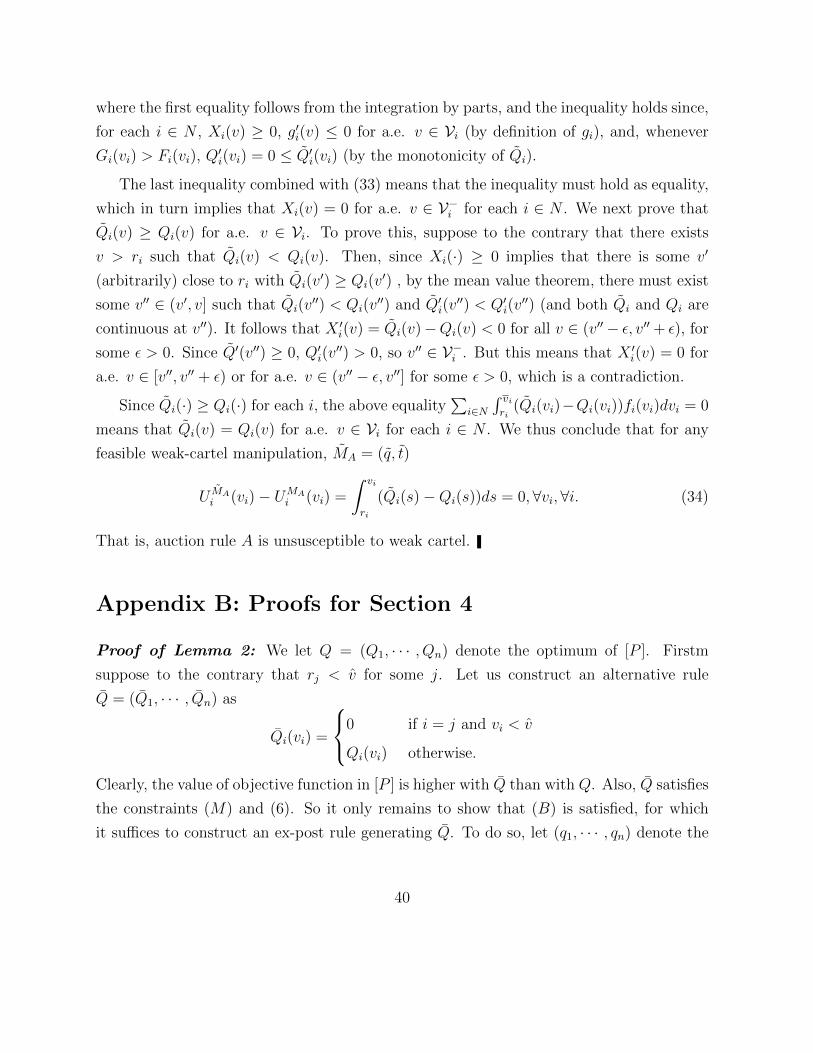
where the first equality follows from the integration by parts, and the inequality holds since,
for each i ∈ N , Xi(v) ≥ 0, g′i(v) ≤ 0 for a.e. v ∈ Vi (by definition of gi), and, whenever
Gi(vi) > Fi(vi), Q′i(vi) = 0 ≤ Q′i(vi) (by the monotonicity of Qi).
The last inequality combined with (33) means that the inequality must hold as equality,
which in turn implies that Xi(v) = 0 for a.e. v ∈ V−i for each i ∈ N . We next prove that
Qi(v) ≥ Qi(v) for a.e. v ∈ Vi. To prove this, suppose to the contrary that there exists
v > ri such that Qi(v) < Qi(v). Then, since Xi(·) ≥ 0 implies that there is some v′
(arbitrarily) close to ri with Qi(v′) ≥ Qi(v
′) , by the mean value theorem, there must exist
some v′′ ∈ (v′, v] such that Qi(v′′) < Qi(v
′′) and Q′i(v′′) < Q′i(v
′′) (and both Qi and Qi are
continuous at v′′). It follows that X ′i(v) = Qi(v)−Qi(v) < 0 for all v ∈ (v′′− ε, v′′ + ε), for
some ε > 0. Since Q′(v′′) ≥ 0, Q′i(v′′) > 0, so v′′ ∈ V−i . But this means that X ′i(v) = 0 for
a.e. v ∈ [v′′, v′′ + ε) or for a.e. v ∈ (v′′ − ε, v′′] for some ε > 0, which is a contradiction.
Since Qi(·) ≥ Qi(·) for each i, the above equality∑
i∈N∫ viri
(Qi(vi)−Qi(vi))fi(vi)dvi = 0
means that Qi(v) = Qi(v) for a.e. v ∈ Vi for each i ∈ N . We thus conclude that for any
feasible weak-cartel manipulation, MA = (q, t)
U MAi (vi)− UMA
i (vi) =
∫ vi
ri
(Qi(s)−Qi(s))ds = 0,∀vi,∀i. (34)
That is, auction rule A is unsusceptible to weak cartel.
Appendix B: Proofs for Section 4
Proof of Lemma 2: We let Q = (Q1, · · · , Qn) denote the optimum of [P ]. Firstm
suppose to the contrary that rj < v for some j. Let us construct an alternative rule
Q = (Q1, · · · , Qn) as
Qi(vi) =
0 if i = j and vi < v
Qi(vi) otherwise.
Clearly, the value of objective function in [P ] is higher with Q than with Q. Also, Q satisfies
the constraints (M) and (6). So it only remains to show that (B) is satisfied, for which
it suffices to construct an ex-post rule generating Q. To do so, let (q1, · · · , qn) denote the
40

ex-post allocation rule for Q and we can construct the ex-post rule for Q as
qi(v) =
0 if i = j and vj < v
qi(v) otherwise.
Second, suppose to the contrary that ri ≥ v∗ for some i ∈ N , that is the object is never
allocated to some bidder whose types are lower than v∗. In this case, consider reducing
slightly ri below v∗. Either (B) does not become binding and then trivially the new auction
is implementable and increases revenue, since J(v) is positive at values slightly below v∗.
Or (B) is binding, in which case it is possible to shift probability away by some player j
toward i and increase the objective, since J(v) is increasing and the same for all players
Proof of Lemma 3: First, let’s define for any v ∈ [v∗, v]
Y (v) := 1− F (v)n −∑i∈N
∫ v
v
Qi(s)f(s)ds. (35)
The function Y (v) represents the probability that the object is not assigned to a bidder
whose value is at least v, even though there exists at least one such bidder. In other words,
Y (v) is the capacity that is not exhausted by the types above v. Given this function and
any subset M ⊂ N , the constraint (B) at a value profile v = (v1, · · · , vn) with vi = ri for
i ∈M and vi = v∗ for i ∈ N\M , can be written as
0 ≤ 1− F (v∗)n−|M |∏i∈M
F (ri)−∑i∈N
∫ v
v∗Qi(v)f(v)dv −
∑i∈M
pi[F (v∗)− F (ri)]
= Y (v∗)−∑i∈M
pi[F (v∗)− F (ri)] + F (v∗)n − F (v∗)n−|M |∏i∈M
F (ri). (36)
Let us relax some constraints of [P ] and consider an alternative problem as follows:
[P ′] max(Q,p,ri)
∑i∈N
∫ v
v∗J(v)Qi(v)f(v)dv +
∑i∈N
pi ·∫ v∗
ri
J(v)f(v)dv
subject to
Y (v) ≥ 0,∀v ∈ [v∗, v] and Y (v) = 0, (37)
41

and ∑i∈M
pi[F (v∗)− F (ri)] ≤ Y (v∗) + F (v∗)n − F (v∗)n−|M |∏i∈M
F (ri),∀M ∈ 2N . (38)
To compare the constraints of [P ′] to those of [P ], note first that the monotonicity
constraint (MN) is dropped in [P ′]. Also, the capacity constraints (B) is imposed on
a much smaller set of value profiles: The inequality in (37) corresponds to the capacity
constraint along the diagonal where vi = v ∈ [v∗, v],∀i ∈ N ; In light of (36), the inequality
(38) corresponds to the capacity constraint at the profile v where vi = ri if i ∈ M and
vi = v∗ otherwise.
To solve [P ′], let us fix r for a while at any level satisfying r (v∗, · · · , v∗). Given
Y (v∗), the second term of the objective function in [P ′] can be independently maximized
as follows: Given Y (v∗) = y for some y ≥ 0,
[R; y] maxpii∈N
∑i∈N
pi ·∫ v∗
ri
J(v)f(v)dv
subject to (38). Let φ(y; r) denote the value function obtained from solving [R; y].
At this point, we need to present the following definitions and result. Define
P :=p = (p1, · · · , pn)
∣∣∣∑i∈S
pi(1− Fi(ri)) ≤ 1−∏
i∈S Fi(ri),∀S ⊂ N. (39)
denote the set of all constant wining probability vectors that are implementable. Note that
the inequalities in (39) corresponds to the capacity constraint associated with the constant
interim allocation rule: Qi(vi) = pi ∈ [0, 1] if vi ≥ ri and Qi(vi) = 0 otherwise. So, P is
the set of all such allocation rules that are implementable (in the sense of being a reduced
form). Clearly, P is a convex polytope since the inequalities defining (39) are all linear.
The following lemma gives a characterization for extreme points of P .
Result 5. A vector p = (p1, · · · , pN) ∈ [0, 1]N is an extreme point of P defined in (39) if
and only if it can be expressed as follows: For some permutation function π : N → N ,
pi =∏
j:π(j)<π(i)
Fj(rj) (40)
with pi = 1 for i = π−1(1). Moreover, at each extreme point, there are exactly n sets,
S1 ( · · · ( Sn, for which (39) is satisfied as equality.
42

Proof. Let us denote by IT , the inequality (39) with S = T ⊂ N . We first show that any
p satisfying (40) is an extreme point of P . Note that the allocation probability p can be
achieved in a feasible way by assigning the k-th order to each agent π(k) and then allocating
the object in this order as long as the agents have values no lower than their reserve prices,
which implies that p is a reduced form. Thus Lemma 1 implies that p must satisfy (39) so
p ∈ PN . Suppose for a contradiction that p is not an extreme point of P . Then, we can
write p = λp′+(1−λ)p′′ for some p′ 6= p and p′′ 6= p. Since pπ(1) = 1 and p′π(1), p′′π(1) ≤ 1 (by
Iπ(1)), we must have p′π(1) = p′′π(1) = 1. Using this and applying Iπ(1),π(2) to p′ and p′′, we
obtain p′π(2), p′′π(2) ≤ Fπ(1)(rπ(1)) = pπ(2), which implies p′π(2) = p′′π(2) = Fπ(1)(rπ(1)) = pπ(2).
Proceeding in this fashion, one can easily verify that p′π(k) = p′′π(k) =∏
j<k Fπ(j)(rπ(j)) = pπ(k)
for all k ∈ N , a contradiction. To show that any extreme point p ∈ P can be expressed as
in (40) for some π, we first establish the following claim.
Claim 3. If for any two sets S, T ⊂ N , IS and IT hold as equality, then either S ⊂ T or
T ⊂ S.
Proof. Suppose for a contradiction that for some S, T ⊂ N , IS and IT hold as equality but
S * T and T * S. Then, we must have S ∩T ( T and S\T 6= ∅. To draw a contradiction,
let us first show ∑i∈T\S
pi(1− Fi(ri)) ≤∏i∈S
Fi(ri)(
1−∏i∈T\S
Fi(ri)). (41)
For this, note that by IS∪T and the assumption,∑i∈S∪T
pi(1− Fi(ri)) ≤ 1−∏i∈S∪T
Fi(ri) (42)∑i∈S
pi(1− Fi(ri)) = 1−∏i∈S
Fi(ri). (43)
It is straightforward to see that (41) results from subtracting (43) from (42) side by side.
Also, by IS∩T , we have ∑i∈S∩T
pi(1− Fi(ri)) ≤ 1−∏i∈S∩T
Fi(ri).
Adding this inequality and (41) side by side yields∑i∈T
pi(1− Fi(ri)) ≤ 1 +∏i∈S
Fi(ri)−∏i∈S∩T
Fi(ri)−∏i∈S∪T
Fi(ri) < 1−∏i∈T
Fi(ri), (44)
43

where the strict inequality follows since S ∩ T ( T and S\T 6= ∅, and thus∏i∈S∩T
Fi(ri) +∏i∈S∪T
Fi(ri)−∏i∈S
Fi(ri)−∏i∈T
Fi(ri)
=( ∏i∈S∩T
Fi(ri)−∏i∈T
Fi(ri))(
1−∏i∈S\T
Fi(ri))> 0.
However, (44) contradicts the assumption that IT holds as equality.
Pick any extreme point p ∈ P satisfying (39). Let us denote by S1, · · · , Sm, all subsets
of N for which (39) is satisfied as equality given p. Due to the above Claim, these subsets
must have a nested structure, that is S1 ⊂ S2 ⊂ · · · ⊂ Sm. Since N contains n elements,
m cannot be greater than n. Suppose for a contradiction that m < n. Then, there must
be some k and h, j ∈ N with h 6= j such that h, j /∈ S` if ` < k and h, j ∈ S` if ` ≥ k. We
now show that p can be obtained by linearly combining some p′ and p′′ ∈ P , contradicting
that p is an extreme point. To do so, we denote by ei, n-dimensional vector with its i-the
element being 1 and all others being zero. Let p′ = p − εeh + δej and p′′ = p + εeh − δej,where ε and δ are sufficiently small positive real numbers satisfying
ε(1− Fh(rh)) = δ(1− Fj(rj)),
which implies that for all ` < k,∑
i∈S` p′i(1−Fi(ri)) =
∑i∈S` pi(1−Fi(ri)) and for all ` ≥ k,∑
i∈S`
p′i(1− Fi(ri)) =∑i∈S`
pi(1− Fi(ri))− ε(1− Fh(rh)) + δ(1− Fj(rj)) =∑i∈S`
pi(1− Fi(ri))
and similarly for p′′. From this, we see that whether p satisfies (39) as equality or strict
inequality, the same is true for p′ and p′′, provided that ε and δ are sufficiently small, which
means p′, p′′ ∈ P . However, p = 12p′ + 1
2p′′, resulting in the desired contradiction. Thus, we
must have m = n, which implies |Sk\Sk−1| = 1 for all k = 1, · · · , n with S0 = ∅.
To complete the proof, define the permutation function π : N → N such that π(i) = k if
i = Sk\Sk−1. Then, by definition of S1, IS1 holds as equality or pi(1−Fi(ri)) = 1−Fi(ri)for i = π−1(1), which yields pi = 1 for i = π−1(1). For an induction argument, suppose
that
pi =∏
j:π(j)<π(i)
Fj(rj) for i = π−1(k′),∀k′ = 1, · · · , k − 1. (45)
44

Then, by definition of Sk and π, we must have for i = π−1(k)∑j:π(j)≤π(i)=k
pj[1− Fj(rj)] = 1−∏
j:π(j)≤π(i)=k
Fj(rj),
which after substituting (45) and canceling the terms, leads us to obtain pi =∏
j:π(j)<π(i) Fj(rj),
as desired.
Claim 4. Given any r (v∗, · · · , v∗), the function φ(·; r) is (weakly) concave and also
satisfies ∂φ(0;r)∂y
< J(v∗).
Proof. To prove the concavity of φ, consider any y and y′, and let p and p′ denote the
solution of [R; y] and [R; y′], respectively. Since the constraint (38) is linear in y and p, for
any λ ∈ [0, 1], we have λp+ (1− λ)p′ satisfying the constraint of [R;λy+ (1− λ)y′]. Given
this and the linearity of the objective function in p, we must have φ(λy + (1 − λ)y′; r) ≥λφ(y; r) + (1− λ)φ(y′; r), as desired.
To prove ∂φ(0;r)∂y
< J(v∗), first redefine N = i ∈ N | ri < v∗ (with some abuse of
notation) and n = |N |. Then, define for each i ∈ N ,
qi :=pi
F (v∗)n−1, G(v) :=
F (v)
F (v∗), and g(v) :=
dG(v)
dv.
Given this, one can rewrite the program [R; y] as
maxqii∈N
F (v∗)n(∑i∈N
qi
∫ v∗
ri
J(v)g(v)dv)
(46)
subject to ∑i∈M
qi[1−G(ri)] ≤y
F (v∗)n+ 1−
∏i∈M
G(ri),∀M ∈ 2N . (47)
Set up the Lagrangian for this problem as
L = F (v∗)n(∑i∈N
qi ·∫ v∗
ri
J(v)g(v)ds)
+∑M∈2N
λM [y
F (v∗)n+ 1−
∏i∈M
G(ri)−∑i∈M
qi[1−G(ri)]],
45
Letting λ0M denote the Lagrangian multiplier when y = 0, by the envelope theorem, we
have ∂φ(0,ri)∂y
= ∂L∂y
=∑M∈2N
λ0M
F (v∗)n. The proof will be done if
∑M∈2N
λ0M
F (v∗)n< J(v∗).
Suppose to the contrary that∑M∈2N
λ0M
F (v∗)n≥ J(v∗). To draw a contradiction, we inves-
tigate the program [R; 0]. First of all, since the objective and constraints are all linear in
(q1, · · · , qn), the optimum arises at one of vertices of the constraint set, which is a polytope
given by the inequalities in (47). Denote that vertex by q0. Note next that the constraints
in (47) are identical to those in (39) with F and pi being replaced by G and qi, respectively.
So, according to Result 5, at the vertex q0, there are exactly n subsets of N , M1, · · · ,Mn,
for which (47) holds as equality, and some j ∈ N for whom j ∈ Mk, ∀k = 1, · · · , n. Also,
letting M := M1, · · · ,Mn, (47) holds as strict inequality for all M ∈ 2N\M, which
implies that λ0M = 0 for M ∈ 2N\M and thus
∑M∈2N λ
0M =
∑M∈M λ0
M . Given this and
y = 0, we have
∂L∂qj
= F (v∗)n∫ v∗
rj
J(v)g(v)ds−∑M∈M
λ0M [1−G(rj)]
= F (v∗)n[1−G(rj)][ ∫ v∗
rj
J(v)g(v)
1−G(rj)ds−
∑M∈2N λ
0M
F (v∗)n
]< F (v∗)n[1−G(rj)]
[J(v∗)−
∑M∈2N λ
0M
F (v∗)n
]≤ 0,
which implies that q0j = 0. This cannot happen, however, due to the fact that the (47)
holds as equality for M = j since j ∈ M.
To understand this result, note that increasing Y (v∗) above 0 means that some winning
probabilities are being transferred from the types above v∗ to the types below v∗.18 While
this transfer will increase the seller’s revenue, φ, from the latter types, Claim 4 says its
marginal impact is smaller than J(v∗), as should be expected. Such transfer, on the other
hand, will entail a loss in the revenue from the types above v∗, which is at least J(v∗). This
implies that at the optimum, the types above v∗ must exhaust their capacity or Y (v∗) = 0.
We now shows that the same is true for all v ≥ v∗. Suppose that ri is fixed at the
optimal level. Then, the allocation rule Q that solves [P ′] can be found as a solution of the
18Since the capacity must be exhausted at the boundary types ri, a decrease in some types’ winning
probability will be matched by an increase in other types’ winning probability.
46

following problem:
[P ′′] maxQi(·)i∈N
∑i∈N
∫ v
v∗J(v)Qi(v)f(v)dv + φ(Y (v∗); r)
subject to (37). Consider this as an optimal control problem with control variable Q(·),state variable Y (·), and salvage value φ(Y (v∗); r). Note that
Y ′(v) = f(v)[∑i∈N
Qi(v)− nF (v)n−1].
Letting γ and λ denote the costate variable and the multiplier for (37), one can write the
Hamiltonian (or Lagrangian) for [P ′′] (exclusive of the salvage value) as
H(v,Q, Y, γ, λ) =∑i∈N
J(v)Qi(v)f(v) + γ(v)f(v)[∑i∈N
Qi(v)− nF (v)n−1]
+ λ(v)Y (v).
Since both objective and constraint functions are concave (in particular, φ(·; r) is concave
by Claim 4), the necessary and sufficient condition for the optimum is given as follows19:
∂H
∂Qi
= (J(v) + γ(v))f(v) = 0, ∀i ∈ N (48)
γ′(v) = −∂H∂Y
= −λ(v) (49)
Y (v∗) ≥ 0, γ(v∗) +∂φ(Y (v∗); r)
∂y≤ 0, and Y (v∗)
[∂φ(Y (v∗); r)
∂y+ γ(v∗)
]= 0 (50)
Y (v), λ(v) ≥ 0 and Y (v)λ(v) = 0, (51)
where γ(v∗) is the derivative of the value function (exclusive of the salvage value) for [P ′′].
From (48), J(v) = −γ(v) and thus using (49), we obtain λ(v) = −γ′(v) = J ′(v) > 0, which
implies by (51) that Y (v) = 0,∀v ∈ [v∗, v]. One can now verify (50) since Y (v∗) = 0 and∂φ(0;r)∂y
< J(v∗) = −γ(v∗) by Lemma 4.
Next, observe that since this feature of the solution holds for problem [P ′] and does not
imply any violation of the extra border constraints or the monotonicity constraint, then it
must also hold at [P ].
Proof of Lemma 4: We first establish the following claim.
19Refer to Leonard and Van Long (1992) or Kamien and Shwartz (1991), for instance.
47
Claim 5. If (B) is binding at some v = (v1, · · · , vn) ∈ V, then we have Qi(vi−) ≤∏j 6=i Fj(vj) ≤ Qi(vi+), where Qi(vi+) = limε→0+ Qi(vi + ε) and Qi(vi−) = limε→0+Qi(vi−
ε);
Proof. Define for any type profile v ∈ V ,
L(v;Q) := 1−∏i∈N
Fi(vi)−∑i∈N
∫ vi
vi
Qi(si)fi(si)dsi. (52)
Note that L(·) is continuous but need not be differentiable where Qi’s are discontinuous.
Given that (B) is binding at v or L(vi, v−i;Q) = 0, we have
vi ∈ arg minsi∈[vi,vi]
L(si, v−i). (53)
This implies that
0 ≤ limε→0+
L(vi + ε, v−i;Q)− L(vi, v−i;Q)
ε= lim
ε→0+
dL(vi + ε, v−i, Q)
dε
= fi(vi)(Qi(vi+)−
∏j 6=i
Fj(vj))
or Qi(vi+) ≥∏
j 6=i Fj(vj). That Qi(vi−) ≤∏
j 6=i Fj(vj) follows similarly.
Consider v ∈ (v∗, v) and suppose to the contrary that Qi(v) > F (v)n−1 for some i.(A
similar argument applies for the case Qi(v) < F (v)n−1.) Then, the above claim implies
that for any v′ > v such that F (v′)n−1 < Qi(v), we must have Qi(v′−) ≤ F (v′)n−1 < Qi(v),
which is a contradiction since Qi(·) is nondecreasing. Thus, Qi(v) = F (v)n−1,∀(v∗, v),∀i ∈N. Given this, the monotonicity of Qi implies that Qi(v) ≥ limε→0Qi(v−ε) = 1 so Qi(v) = 1
since Qi(v) cannot exceed 1.
Proof of Lemma 5:
By Lemma 3, whatever r is chosen, we must have Y (v∗) = 0 at the optimum. Thus,
in order for (p, r) to solve [P ′], the pair (q, r) must solve the problem given by (46) and
(47) with y = 0 and r being included as choice variable. As mentioned in Result 4, the
optimum of that problem arises at one of the vertices in the constraint set. This implies
that given any vector r, we can relabel the (symmetric) bidders so that qi =∏i−1
k=1G(rk)
48

or pi = F (v∗)n−1qi = F (v∗)n−i∏i−1
k=1 F (rk). Plugging this into (46) yields the objective
function in (8), which can then be maximized by choosing r optimally.
We now show that v = rn < rn−1 < · · · < r1 < v∗. Define first
Πn :=
∫ v∗
rn
J(v)f(v)dv, (54)
and define recursively
Πi(ri, Πi+1) := F (v∗)n−i∫ v∗
ri
J(v)f(v)dv + F (ri)Πi+1, i = 1, · · · , n− 1.
One can easily verify that the objective function in (8) is the same as the function Π1 defined
above. Also, the terms in the objective function that involve ri are entirely represented
by Πi (multiplied by some expression unrelated to ri.). Thus, maximizing the objective
function corresponds to choosing ri for each i ∈ N that maximizes Πi, given the maximized
value of Πi+1. Let us recursively define ri and Πi to be respectively the maximizer and
maximized value of Πi with Πi+1 given. From (54), it is immediate that rn = v.
In order to complete the proof, we adopt the induction argument to show the followings:
For all i = 1, · · · , n − 1, (i) Πi+1 < F (v∗)n−iJ(v∗); (ii) ri+1 < ri < v∗. Consider i = n − 1
for the initial step. Then, Πn =∫ v∗vJ(s)f(s)ds < F (v∗)J(v∗) so (i) is satisfied. For (ii),
note that ∂Πn−1(rn−1,Πn)∂rn−1
= f(rn−1)[Πn − F (v∗)J(rn−1)], which is negative if rn−1 = v∗ and
positive if rn−1 = v = rn. So we must have rn < rn−1 < v∗. Let us now assume that (i)
and (ii) hold for some k > 1, that is Πk+1 < F (v∗)n−kJ(v∗) and rk+1 < rk < v∗. We show
that Πk < F (v∗)n−k+1J(v∗) and rk < rk−1 < v∗. First, the fact that Πk < F (v∗)n−k+1J(v∗)
follows from
Πk − F (v∗)n−k+1J(v∗) = F (rk)Πk+1 − F (v∗)n−k+1J(v∗) + F (v∗)n−k∫ v∗
rk
J(v)f(v)dv
< F (v∗)n−k[J(v∗)(F (rk)− F (v∗)) +
∫ v∗
rk
J(v)f(v)dv]< 0, (55)
where the first inequality is due to the inductive assumption and the second inequality
holds since v∗ > rk and J(v∗) > J(v),∀v < v∗. To show rk−1 < v∗, note that by (55),∂Πk−1(v∗,Πk)
∂rk−1= f(v∗)[Πk − F (v∗)n−k+1J(v∗)] < 0, which implies rk−1 < v∗. To show lastly
that rk < rk−1, notice that the first-order conditions w.r.t. rk and rk−1 yield J(rk) =
49

Πk+1
F (v∗)n−kand J(rk−1) = Πk
F (v∗)n−k+1 , respectively. So the result will follow if Πk+1
F (v∗)n−k<
ΠkF (v∗)n−k+1 or F (v∗)Πk+1 < Πk, which is true since Πk = Πk(rk,Πk+1) > Πk(v
∗,Πk+1) =
F (v∗)Πk+1.
Proof of Proposition 1: Assuming the symmetry of allocation rule Qi(·) = Q(·), we
can express the seller’s revenue maximization problem as20:
[Ps] maxQ:[v,v]→[0,1]
n
∫ v
v
J(v)Q(v)f(v)dv
subject to [M ], ∫ v
v
Q(s)f(s)ds ≤ 1− F (v)n
n, ∀v ∈ [v, v], (56)
and Q′(v) = 0, ∀v ∈ [r, v∗). (57)
Note that (56) is the capacity constraint for the symmetric auction rule (which follows from
Border) while (57) is the collusion-proofness constraint. The proof hereafter follows the
steps similar to the ones we took in Lemma 4 through 4.
Letting p = Q(v),∀v ∈ [v, v∗) and defining as in (35)
Y (v) = 1− F (v)n − n∫ v
v
Q(s)f(s)ds,
we write a relaxed program
[P ′s] maxQ:[v,v]→[0,1]
n
∫ v
v∗J(v)Q(v)f(v)dv + np
∫ v∗
r
J(v)f(v)dv
subject to
Y (v) ≥ 0, ∀v ∈ [v∗, v], and Y (v) = 0 (58)
and np[F (v∗)− F (r)] ≤ Y (v∗) + F (v∗)n − F (r)n. (59)
Here (58) and (59) are the capacity constraint (56) applied at v ∈ [v∗, v] and v = r,
respectively. Taking r as given and fixing Y (v∗) = y, let
φ(y; r) = maxp
np
∫ v∗
r
J(v)f(v)dv (60)
20Here U(v) has already been set at zero for the optimality.
50

subject to
np[F (v∗)− F (r)] ≤ y + F (v∗)n − F (r)n. (61)
One can easily verify that φ(·, r) is concave and ∂φ(0;r)∂y
< J(v∗).
Now we can replace by φ(Y (v∗); r) the second term of the objective function in [P ′s] and
eliminate the constraint (59). So the program [P ′s] can be turned into an optimal control
problem with with control variable Q(·), state variable Y (·), and salvage value φ(Y (v∗); r),
whose Hamiltonian is written as
H(v,Q, Y, γ, λ) = nJ(v)Q(v)f(v) + γ(v)nf(v)[Q(v)− F (v)n−1
]+ λ(v)Y (v).
From this, one can obtain the same first-order conditions as in (48) to (51), which are
necessary and sufficient for the optimum, given the concavity of the program. Also using
the same argument as the one following (51), it can be seen that Y (v) = 0,∀v ∈ [v∗, v].
From this, it follows that Q(v) = F (v)n−1,∀v ∈ [v∗, v]. Since the constraint (61) must be
binding with Y (v∗) = y = 0, we have
p =F (v∗)n − F (r)n
n[F (v∗)− F (r)]=
∑ni=1 F (v∗)n−iF (r)i−1
n. (62)
Plugging this into (60) and maximizing φ(0; r) with respect to r yields rs, which in turn
can be substituted into (62) to yield ps. It is straightforward that the ex-post allocation
described in (12) yields the desired interim allocation.
Proof of Proposition 2: Given the interim winning probability profile (p1, · · · , pn), the
capacity constraint (B) is the same as requiring p ∈ P defined in (39). Then, using the
characterization in Lemma 5, we can express any p ∈ P as a convex combination of extreme
points given in (40). In other words, letting pπi :=∏
j:π(j)<π(i) Fi(ri) and pπ = (pπ1 , · · · , pπn),
we can find some weighting vector (λπ)π∈Π ∈ ∆Π for each p ∈ P such that
p =∑π∈Π
λπpπ.
Given this, (13) can be rewritten as
max(λπ)π∈Π(ri)i∈N
∑π∈Π
λπ∑i∈N
pπi ri(1− Fi(ri))
51

= max(λπ)π∈Π
∑π∈Π
λπ[
max(ri)i∈N
∑i∈N
pπi ri(1− Fi(ri))]
= maxπ∈Π
[max
(ri)i∈N
∑i∈N
pπi ri(1− Fi(ri))]
(63)
as desired, where the second equality follows since the objective function is linear with
respect to the weighting vector (λπ)π∈Π so the entire weight can be be assigned to a function
π that maximizes the term in the square bracket.
References
[1] Athey, S. and K. Bagwell (2008): “ Collusion with Persistent Cost Shocks,”
Econometrica, 76, 493-540.
[2] Border, K.C. (1991): “Implementation of Reduced Form Auctions: A Geometric
Approach,” Econometrica, 59, 1175-1187.
[3] Border, K.C. (2007): “Reduced Form Auctions Revisited,” Economic Theory, 31,
167-181.
[4] Che, Y.-K. and J. Kim (2006): “Robustly Collusion-Proof Implementation,” Econo-
metrica, 74, 1063-1107.
[5] Che, Y.-K. and J. Kim (2009): “Optimal Collusion-Proof Auctions,” Journal of
Economic Theory, 144, 565-603.
[6] Condorelli, D (2009): “What money can’t buy: allocations with priority lists,
lotteries and queues” mimeo Northwestern University 144, 565-603.
[7] Doree, A.G. (2004): “Collusion in the Dutch Construction Industry: An Industrial
Organization Perspective,” Building Research & Information 32(2), 146-156.
[8] Kamien, M. and N. Schwartz (1980): “ Dynamic Optimization: The Calculus of
Variations and Optimal Control in Economics and Management” North Holland.
[9] Krishna, V.:(2009) “Auction Theory,” Academic Press.
52

[10] Leonard, D. and N. Van Long (1992): “Optimal Control Theory and Static
Optimization in Economics ,” Cambridge University Press.
[11] Laffont, J.-J. and D. Martimort (1997): “Collusion under Asymmetric Infor-
mation,” Econometrica, 65, 875-911.
[12] Laffont, J.-J. and D. Martimort (2000): “Mechanism Design with Collusion
and Correlation,” Econometrica, 68, 309-342.
[13] McAfee, R.P. and J. McMilan (1992): “Bidding Rings,” American Economic
Review, 82, 579-599.
[14] Myerson, M. (1981): “Optimal Auction Design,” Mathematics of Operations Re-
search, 6, 58-73.
[15] Pavlov, G. (2008): “Auction Design in the Presence of Collusion,” Theoretical Eco-
nomics, 3, 383-429.
[16] Pesendorfer, M. (2000): “A Study of Collusion in First-price Auctions,” Review
of Economic Studies, 67, 381-411.
53


