Loughborough UniversityInstitutional Repository
Water bath modelling oftransient and timedependent naturalventilation flows
This item was submitted to Loughborough University's Institutional Repositoryby the/an author.
Additional Information:
• A Doctoral Thesis. Submitted in partial fulfillment of the requirementsfor the award of Doctor of Philosophy of Loughborough University.
Metadata Record: https://dspace.lboro.ac.uk/2134/23245
Publisher: c© Stephen Philip Todd
Rights: This work is made available according to the conditions of the Cre-ative Commons Attribution-NonCommercial-NoDerivatives 4.0 International(CC BY-NC-ND 4.0) licence. Full details of this licence are available at:https://creativecommons.org/licenses/by-nc-nd/4.0/
Please cite the published version.
School of Civil and Building Engineering
Water Bath Modelling of Transient and Time Dependent Natural Ventilation Flows
by
Stephen Philip Todd
Submitted in partial fulfilment of the requirements for the award of
Doctoral Thesis of Loughborough University
July 2016
© Stephen Philip Todd 2016

i
Abstract
Since electricity was first harnessed, humanity has developed a lifestyle which can
not exist without it. Traditionally, electricity has been created by burning fossil fuels
which produces waste gases including carbon dioxide. These waste gases have
accumulated in our atmosphere and are theorised to have contributed to a warming
of the earth, causing a 0.4°C rise in average surface temperature since the 1970’s
(DECC 2013). A warming of the earth is thought to lead to increased frequency of
catastrophic weather events such as droughts and heat waves, leading to many
deaths (Met Office 2015).
In recent years, there has been a drive to reduce our dependence on the burning of
fossil fuels by making technologies more efficient, developing methods of electricity
generation which do not involve the burning of fossil fuels as well as replacing
techniques requiring high energy demands with low energy techniques. Natural
ventilation is one such low energy technique which can replace more electricity
intensive strategies such as mechanical ventilation and air conditioning whilst still
ensuring a room which is neither too cold nor too warm and removes pollutants.
Natural ventilation (NV) has smaller driving forces than mechanical ventilation and
air conditioning techniques. As a result, wind, location of heat sources and/or
openings and even the room geometry can influence any internal natural air flow
patterns, potentially causing a NV strategy to behave in a way for which it was not
designed. In the event of such circumstances, this can lead to a naturally ventilated
room becoming much warmer or much colder than what an occupant would find
comfortable and in such events, the NV strategy's ability to remove pollutants from
the space may also reduce, which can be detrimental to the occupants health. Such
unintended consequences are not desirable and should be avoided where ever
possible. Understanding how NV strategies can behave in ways that is not intended
is important to ensure that NV is a strategy which can replace more electricity
intensive ventilation strategies.
To better understand NV, physical modelling techniques can be employed. One
technique, known as water bath modelling (WBM) uses salt water and fresh water to
simulate the density differences between ambient and warmer than ambient air. This
study uses WBM to better understand NV, specifically looking at traditional and non-

ii
traditional NV strategies along with simulating circumstances which can cause a NV
strategy to behave in an unintended way.
Initially, comparisons are made between simple simulations within the WBM facility
at Loughborough University with current NV theory to provide confidence that results
from more complicated scenarios represent real life scenarios. Results from simple
scenarios were generally shown to agree closely with NV theory and results from
previous researches. For scenarios where there was no agreement, explanations are
provided based on visual observations and data collected during WBM simulations.
Simulations conducted within this research show the importance of any interactions
between incoming ambient fluid, heat sources, internal geometry of the space and
air flow patterns. Such interactions were shown to cause significant change in
temperatures within the space, leading to results disagreeing with theoretical
predictions. The consequences of such interactions were also shown to significantly
increase the time required for the ventilation strategy to fully purge the space of
warmer-than-ambient air when all heat sources leave the room. A temporary gust of
wind was shown to be able to overpower the buoyancy forces of a NV strategy such
that the air flow patterns within the space would fundamentally change, resulting in
very different internal temperatures. The position of a heat source was also shown to
be of great significance, with different interactions occurring between the heat source
locations resulting in different temperatures within the space.
Perhaps most importantly, this research has shown that the location of openings can
be more critical than the number of openings. A room with well placed openings was
shown to have lower internal temperatures than an identical room with double the
number of openings placed in a different position.
Considerable insight has been gained into the complexities of NV. Further
understanding has also been achieved for scenarios which can cause NV strategies
to behave in fundamentally different ways than intended and the work presented
within this research suggests ways to reduce such risks, increasing the applicability
of NV within buildings, therefore reducing the energy requirements from buildings.

iii
Acknowledgements
I would like to firstly thank Mark Harrod, Mick Barker, Jayshree Bhuptani, Geoffrey
Russel and Mick Shonk who are the lab technicians at Loughborough University who
helped build the foundations of my experiments. Without them, I would not have
been able to produce the results that I have
Secondly, my Ph.D supervisor, Prof. Malcolm Cook who gave me considerable trust,
understanding, support and time. You gave me the chance to fulfil one of my biggest
dreams (to get a doctorate) and every step of the way you were there to help me.
Thirdly, I would like to thank my parents. You taught me to always aim high and
regardless of any situation I may be in, you gave me the skills, support and the
strength to achieve all that I have. In particular, I enjoyed our late night conversations
when trying to solve a physical problem
Lastly, I would like to thank my partner, Gloria who has given me considerable help
and support throughout the process of this research. Whilst the PhD has been
difficult and you have often borne the brunt of it, you have always been strong.
Without you all, I would not have been able to complete this research and therefore
one of my life long ambitions, thank you.

iv
List of figures
Figure 1.1.Natural Ventilation strategies and principles.
Figure 1.2.Water bath modelling simulation.
Figure 2.1.Wind and temperature driven Natural Ventilation
Figure 2.2. Principle forces acting upon a particle.
Figure 2.3.Principles of buoyancy-driven Natural Ventilation with a single heat source.
Figure 2.4.Basic Natural Ventilation Strategies: a) Single opening, b) cross
ventilation and c) stack natural ventilation.
Figure 2.5. Pressure variation with height within a stack ventilated room, where '+'
refers to an area of higher pressure and '-' refers to an area of lower pressure.
Figure 2.6. Emptying space, initially filled with warmer than ambient air based on a
night purging strategy.
Figure 2.7. Four possible flow regimes for an emptying space.
Figure 2.8. Pictures of a space emptying with flow regime 2. Figure a), b), c) and d) show draining at times 0, 15, 60 and 120 seconds consecutively where time to empty, te = 375s.
Figure 2.9. Pictures of a space emptying with flow regime 3. Figure a), b), c) and d)
show draining at times 0, 140, 280 and 350 seconds consecutively where time to
empty, te = 700s.
Figure 2.10. Pictures of a space emptying with flow regime 4. Figure 1), b) and c)
show draining at times 0, 480 and 1200s consecutively where time to empty, te=
16000s.
Figure 2.11.Displacement ventilation with a continuous single point source.
Figure 2.12.Virtual origin of a heat source.
Figure 2.13.Displacement ventilation with two heat sources of different strengths.
Figure 2.14.The merging of two identical plumes separated by some distance Xo.

v
Figure 2.15. Flow regimes for a room with a single point heat source within it, venting into a large atrium with an outlet at high level. The atrium contained no inlet in a), but contained a low level inlet in b).
Figure 2.16.An area heat source showing the effect of ‘necking’.
Figure 2.17.a) A schematic of an experimental set-up used to form a turbulent lazy plume over a large area with a water bath using brine and b) the resulting brine plume flowing out of the nozzle.
Figure 2.18.Measured temperatures within a model simulating an area ‘cold source’.
Figure 2.19. Possible NV flow regimes with the interaction of wind, a) wind reinforcing buoyancy, b) a weak wind opposing buoyancy, and c) a strong wind opposing buoyancy, and causing a change in flow direction
Figure 2.20.Effect of strong opposing wind from WBM using salt.
Figure 2.21. Experimental set up to simulate wind in WBM using salt.
Figure 2.22. Water bath modelling showing how a change in the buoyancy of a brine source causes a temporary change in interface height. With non-dimensional time as the x-axis, and non-dimensional height of the interface as the y axis.
Figure 2.23.Effect of source strength being changed from its original strength (In orange) to an increased strength (blue).
Figure 2.24. The transient changes of two simulations with different heat sources within an identical model with time.
Figure 2.25.Water bath modelling showing the development of transitional flows during pre-cooling of a room.
Figure 2.26.Formation of four different flow regimes in a pre-heated room.
Figure 2.27.The four different transitional flows which can form depending on the opening area (A) and the reduced gravity of the original fluid within the space g1.
Figure 2.28.The effect on interface height within a room with a heat source and distributed cooling on the ceiling.
Figure 2.29. Three possible flow regimes within the same space. Arrows indicate direction of flow through openings
Figure 2.30.Theoretical and experimental dimensionless room temperatures for each
of the three regimes depending on the area of the bottom opening.
Figure 2.31. Possible flow regimes for two interconnected rooms with identical area
heat sources and openings at high level.
vi
Figure 2.32. Flow regime and development of internal temperatures within
geometrically identical interconnected rooms with different area heat sources.
Figure 2.33.Temperature within room A and B depending on the history of flow with varying heat source strength in room A.
Figure 2.34. Change in flow regime and internal temperatures when the heat source
strength of the upstream room is increased.
Figure 3.1. Plume formation for: a) A hot air plume caused by a human within a room,
b) a heated wire (Orange box) heating water around it and c) brine is fed into the
model filled with water by a pipe.
Figure 3.2. Experimental set up of water bath facility at Loughborough University.
Figure 3.3.Build-up of brine (dyed red) in the large acrylic tank during a simulation.
Figure 3.4. Experimental set up allowing for removal of brine and replacement with
fresh water during a simulation. Not to scale
Figure 3.5.Reservoir tank for storage and continued mixing of brine during water
bath simulations.
Figure 3.6.Header tank with visible over-flow pipe, allowing for a constant head
within the system, providing a constant flow rate.
Figure 3.7. Analogue flow meter, used for manual control of the flow rate of brine into
the model
Figure 3.8. Variations in colour observed when using a red food dye.
Figure 3.9.The effect of a brine plume being laminar instead of turbulent for a
distance ‘x’ on the interface.
Figure 3.10.Flow of brine from nozzle showing transition from laminar to turbulent
flow. a) High speed plume exiting from a pipe, b) Slow speed plume exiting from the
same pipe as in a).
Figure 3.11.Objects were inserted into the tip of the pipe where brine flowed into the
model in an attempt to induce turbulence.
vii
Figure 3.12. Nozzles with the intent to induce turbulent flow into a fluid exiting the
nozzle. a) nozzle schematic (Source J. McCarthy and A. Molloy 1974), b) Standard
plastic nozzle (Often used with silicone tubes) with similar characteristics to the
nozzle schematic in a).
Figure 3.13.Nozzle design for inducing turbulence into fluid which allows for virtual
origin corrections.
Figure 3.14.Change in laminar region of plume depending on mesh size within
nozzle design used by Hunt and Linden (2001). (a) 40µm mesh, (b) 75 µm mesh, (c)
2 pieces of 75µm mesh on top of each other, (d) 200 µm mesh.
Figure 3.15. Cap with 200 µm mesh and a nut glued to it to form a nozzle with the
dimensions described by Hunt and Linden (2001) to form a turbulent plume.
Figure 3.16. Mesh blocked with particulates and algae.
Figure 3.17. Placement of nozzle and effect on plume development, a) nozzle is
placed on the outside of the model and b) nozzle is placed within the perspex.
Figure 3.18. Ruler attached to model to allow for height readings during experiments.
Figure 3.19. View of brine within model when eye level is (a) above interface height,
(b) below interface height and (c) at interface height level. The top of the brine is
marked in red.
Figure 3.20. Anton Parr DM-35a density meter used to sample and measure fluid
density.
Figure 3.21. Set up of conductivity probes and meters.
Figure 3.22.Conductivity to density conversion chart.
Figure 3.23. Conductivities measured during a draining simulation
Figure 3.24. Possible temperature/density gradients within a naturally ventilated
model, (a) vertical gradient and (b) diagonal gradient
Figure 3.25. Schematic for Schleiren double pass technique
Figure 3.26. Artificial Schlieren set up.

viii
Figure 3.27. Resulting detectable diffraction depending on line sizing on mask where
(a) lines are too thin, (b) lines are too thick and (c) lines are perfectly sized.
Figure 3.28. Schlieren photograph of brine plume flowing through model.
Figure 3.29.Schlieren photograph of disruption of the interface due to incoming
ambient fluid from low level (see section 5.2.5.3).
Figure 4.1.Photographs and diagrams of Benchmark 1, the ‘simple’ box used to
validate the water bath facility. Internal dimensions given where appropriate.
Figure 4.2 shows the normalised converted density, ρ of the water within the
tank but outside of the model during a simulation.
Figure 4.3.Converted density profile of test simulation at position P2.
Figure 4.4. 4No. filling density profiles at P2 with an undisturbed plume.
Figure 4.5.Filling density profiles at P1 and P2 with a disturbed plume.
Figure 4.6.Draining methodology 1 and 2.
Figure 4.7.Interface heights following draining methodology 1 when initially a) fully
filled and b) partially filled.
Figure 4.8. Interface heights during draining following methodology 1.
Figure 4.9.Interface heights during draining following methodology 1 with 4No. side
openings at low and high level.
Figure 4.10.Interface heights during draining following methodology 2 with 2No. side
openings at low and high level.
Figure 4.11.Interface heights during draining following methodology 2 with 4No.
lower side openings and 2No. upper side openings.
Figure 4.12.Interface heights during draining following methodology 2 with 4No. side
openings at low and high level.
Figure 4.13.Interface heights and internal densities at high level during draining
following methodology 1 with 2No. side openings at low and high level.

ix
Figure 4.14.Density profile of a steady displacement flow
Figure 4.15. Different H measurements used for theoretical and experimental
comparisons for interface height and density. Diagram not to scale.
Figure 4.16.Depth of ambient layer for displacement ventilation where a) there is a
negligible mixed layer and b) where there is a significant mixed layer below the
interface.
Figure 5.1. Density 'filling' profiles for non-disturbed heat sources with side openings
at high and low level.
Figure 5.2.The side openings in line with the location of the plume with a) and b)
showing different side view points.
Figure 5.3.Densities measured at P1 and P2 for filling simulations with side openings.
Figure 5.4. Disturbance of brine plume with time during a simulation
Figure 5.5.Measured densities during filling for i) at P2 and ii) at P1 for simulations
with openings on the floor and ceiling.
Figure 5.6. Diagram showing how increased F through space leads to greater
penetration of ambient fluid from inlet which can lead to completed disruption of
interface.
Figure 5.7. Measured densities during filling for i) at P2 and ii) at P1 for simulations
with openings on the floor and ceiling with stacks.
Figure 5.8. Densities profiles at P1 and P2 for 2No. openings located on each side.
Figure 5.9.Densities at P1 and P2 for side simulations with 4No. lower openings and
4No. upper openings.
Figure 5.10.Density profile at P1 and P2 for simulations with 1No.openings on the
floor and ceiling.
Figure 5.11.Density profile at P1 and P2 for simulations with 2No.openings on the
floor and ceiling.
Figure 5.12.Density profile at P1 and P2 with 3No.openings on the floor and ceiling.

x
Figure 5.13.Density profile at P1 and P2 with 4No. openings on the floor and ceiling.
Figure 5.14. Filling simulations with openings on the side or on the floor and ceiling
which have two inlets and two outlets
Figure 5.15.Filling simulations with openings on the side or on the floor and ceiling
which have 4No. openings at low and high level.
Figure 5.16. Draining simulations with 2 lower and 2 upper openings at a) densities
recorded at P2 and b) densities recorded at P1
Figure 5.17.Penetration of incoming ambient fluid through a draining simulation with
openings on the top and bottom of the model.
Figure 5.18. Draining simulations with 4 lower and 4 upper openings at a) densities
recorded at P2 and b) densities recorded at P1
Figure 6.1. A naturally ventilated space where a), the driving forces are undisturbed
by external forces, b) driving forces are reduced in strength by a weak wind and c)
where driving forces are overpowered and the flow regime is fundamentally changed.
The size of an arrow represents the quantity of air flowing through an opening.
Figure 6.2. Three possible flow regimes, arrows show direction of fluid flow.
Figure 6.3. Diagram of model used to produce 'mechanically induced' time
dependant flows.
Figure 6.4 Flow diagram for the three flow regimes where the large arrows state the
required action to force flow regime change.
Figure 6.5.Density measurements during flow regime transitions.
Figure 6.6. Emptying simulation with densities at low and high level with flow regime
automatically changing.
Figure 7.1: Internal dimensions of (a) Picture of model and (b) the Perspex model at scale 1:20
Figure 7.2.Plan view of hospital model with number locations of heat sources.

xi
Figure 6.3: Transitional development of internal thermal environment shown in
clockwise direction from (a) initialisation to (d) attainment of maximum interface
height.
Figure 7.4. The scaled model at steady state (arrow indicates flow of fresh air from
the duct) for the scenario where there is one heat source at position 1.
Figure 7.5: The interface layer in (a) WBM and (b) CFD equivalent
Figure 7.6: Formation of build up of fluid around the duct in (a) CFD and (b) WBM .
Figure 7.7. Density profile for scenarios where individual heat sources are within the
space where a) density recorded at high level and b) density recorded at low level.
Figure 7.8.Development of flow characteristics for heat source location 3. The size
and direction of the blue arrow represents the relative strength and direction of
incoming ambient fluid.
Figure 7.9.Converted densities at a) high level and b) low level during the draining of
scenarios.
Figure 8.1.Opening strategies for filling simulations used in Chapter 4 and 5.
Figure 8.2. Three possible flow regimes for model used in Chapter 6
Figure 8.3.Benchmark 3 model.
Figure 8.4.Theatre model which was intended to form Benchmark 4.
List of Tables

xii
Table4.1.Theoretical and experimental data for interface heights and densities for
different opening arrangements.* refers to simulation where upper opening had its
area reduced by 50% to allow for another simulation.
Table 5.2. Speed of incoming ambient fluid into the model when disruption to
interface occurs with openings on the floor and ceiling of the model.
Table 5.3.Speed of incoming fluid through when significant disruption to interface
occurs with openings on the floor and ceiling.
Table 5.4.Speed of incoming fluid through when disruption to interface occurs with
openings on the floor and stacks on the ceiling.
Table 5.5. Speed of incoming fluid through when significant disruption to interface
occurs with openings on the floor and stacks on the ceiling.
Table 5.6Speed of incoming fluid through when significant disruption to interface
occurs with openings on the floor and ceiling.
Table 5.7.Experimental and theoretical data for density and time to reach steady
state for simulations with openings on the bottom and top of model.
Table 6.1.Predictions for flow regime A, B and C to occur with varying effective lower
opening area.
Table 6.2. Experimental regimes observed with varying lower opening area.
Table 7.1.Converted densities at high and low level for individual heat source
scenarios.
Table 7.2.Region of protraction for each of the four simulations.
List of symbols

xiii
A Opening area (m2)
An Nozzle opening area (cm2)
A* Effective opening area
Ar Archimedes number
b0 Radius of large area plume at floor level (cm)
B Buoyancy (m4s-3)
B1 Buoyancy of plume 1 (m4s-3)
B2 Buoyancy of plume 2 (m4s-3)
Bf Initial buoyancy of plume
C Entrainment coefficient
Cd Discharge coefficient
Ce Coefficient of expansion (K-1)
Cp Specific heat capacity (kJ/kg K)
d Internal diameter of a nozzle (cm)
dc Diameter of nozzle after contraction (cm)
F Volume flux
f Denotes full scale
g Acceleration due to gravity (9.81 m/s2)
g’ Reduced gravity (m/s2)
h Height of the interface (m)
h1 Height of lower interface (m)
h2 Height of upper interface (m)
H Height between lower opening and upper opening (m)
Ha Height of atrium (m)
Hx Distance from the plume source ‘x’ (m)
Ln Length of nozzle (cm)
La Source flow rate length (cm)
Lm Momentum jet length (cm)
Lq Length scale (m)

xiv
m Denotes model scale
M Momentum (cm4s-2)
Pe Peclet numbers
Pr Prandtl Number
Q Flow rate (cm3/s)
Qx Flow rate at height ‘x’ (cm3/s)
Qper opening Flow rate through individual opening of model (cm3/s)
P Pressure (Pa)
R Ratio of lower opening and upper opening areas
Re Reynolds numbers
S Floor area of the space (m2)
T Temperature (K)
Ta Ambient temperature (K)
T0 Initial temperature (K)
t Time taken (s)
td Time spent draining (s)
te Time to empty (s)
tss Time to steady state (s)
tts Timescale to converge to steady state
u Velocity of fluid (m/s)
uper opening Velocity of fluid (m/s)
kinematic viscosity of the fluid (m2/s)
V Volume of a space (m3)
W Heat flux produced from the heat source (W)
X Length travelled by the plume (m)
X0 Horizontal distance between plumes (cm)
z Height between the interface and the NPL (m)
Zm The vertical height at which two plumes merge (cm)
z*avs Asymptotic virtual origin (cm)

xv
The change in.
λt Temperature coefficient
ξ0 Ratio between interface height and height between lower and upper openings
ξa Non-dimensional opening area
ξb Non-dimensional buoyancy flux
ξh Non-dimensions interface height
ξq Non-dimensional flow rate
ξt Non-dimensional temperature
ξRatiobetweendistancefromtheplumesourceandlengthscale
Density (kg/m3)
0 Initial density (kg/m3)
normalised Normalised density (kg/m3)
Coefficient of expansion (T-1)
δ Non-dimensional reduced gravity of the Buoyant Layer
δinitial Non-dimensional reduced gravity of the initially buoyant layer
Entrainment constant
αc Angle of convergence (°)
αtd Thermal diffusivity (m2/s)
Γ Source parameter
Π PI
λ Ratio of height and height at which 2 plumes merge (cm)
μ Dynamic viscosity (kg/m.s)
Dimensionless time for temperature to converge to steady state
Glossary and abbreviations
xvi
BRI – Building Related Illness
CFD – Computational Fluid Dynamics
CO2 – Carbon dioxide
GHG – Greenhouse gases
HVAC – Heating, ventilation and air conditioning
MRT – Mean radiant temperature
NPL – Neutral pressure level
NV – Natural ventilation
PMV – Predictive Mean Vote
SBS – Sick Building Syndrome
UK – United Kingdom
VOC’s - Volatile Organic Compounds
WBM – Water Bath Modelling
xvii
Table of Contents
Chapter 1. Introduction ........................................................................................................................ 1
1.1 Background ................................................................................................................... 1
1.2 Natural Ventilation ........................................................................................................ 3
1.3 Water Bath Modelling ................................................................................................... 4
1.4 Justifications for work ................................................................................................... 5
1.5 Aims and Objectives .................................................................................................... 6
1.6 Contribution to knowledge ........................................................................................... 7
Chapter 2. Literature Review and Background Theory .................................................................. 8
2.1 Preamble ........................................................................................................................ 8
2.2 Designing a thermally comfortable and healthy building ........................................ 8
2.3 Low energy building design ...................................................................................... 10
2.4 Natural ventilation ....................................................................................................... 11
2.5 Simulating Natural Ventilation .................................................................................. 14
2.6 Principles of buoyancy driven natural ventilation ................................................... 16
2.7 Analytical Models for Natural Ventilation and Plume Theory ............................... 20
2.7.1 Emptying space with no continuous heat source ........................................................ 20
2.7.2 Emptying space with continuous heat sources ............................................................ 27
2.7.2.1 Single heat source .................................................................................................... 27
2.7.2.2 Virtual origin ............................................................................................................... 29
2.7.2.3 Two heat sources within a room which do not interact ....................................... 32
2.7.2.4 Interacting turbulent plumes with identical buoyancies ....................................... 34
2.7.2.5 Interconnected spaces ............................................................................................. 36
2.7.2.6 Open area heat source ............................................................................................ 37
2.8 Transient and time dependant flows ........................................................................ 40
2.8.1 Time dependant and transient air flows caused by the effect of wind. .................... 41
2.8.2 Time dependent and transient flows caused by effects other than wind ................. 44
2.8.2.1 Transient Flows ......................................................................................................... 44
2.8.2.2 Summary of Transient Flows .................................................................................. 53
2.8.2.3 Time dependant flows .............................................................................................. 54
2.8.2.3 Summary of time dependant flows ......................................................................... 60
2.9 Conclusion of Chapter ............................................................................................... 61
Chapter 3. Experimental set up and methodology ........................................................................ 62
xviii
3.1 Preamble ...................................................................................................................... 62
3.2 Introduction .................................................................................................................. 62
3.3 Scaling equations ....................................................................................................... 64
3.3.1 Exact simulation scaling .................................................................................................. 64
3.3.2 Non dimensional scaling ................................................................................................. 70
3.4. Experimental set up .................................................................................................. 70
3.4.1 Large water reservoir ....................................................................................................... 72
3.4.2 Reservoir tank ................................................................................................................... 73
3.4.3 Pumps ................................................................................................................................ 75
3.4.4 Header tank and flow meter............................................................................................ 75
3.4.5 Dyes ................................................................................................................................... 77
3.4.6 Nozzles and permeable plates. ...................................................................................... 78
3.4.7 Measuring interface heights within the model .............................................................. 87
3.5 Density and conductivity measuring devices ......................................................... 88
3.5.1 Anton Parr DM-35a density meter ................................................................................. 88
3.5.2 Conductivity probes. ........................................................................................................ 89
3.6 Photography ................................................................................................................ 93
3.6.1 Schlieren camera technique ........................................................................................... 94
3.6.2 Artificial Schlieren ............................................................................................................. 96
Chapter 4. Benchmark 1 (Simple box) - Validation ..................................................................... 100
4.1 Preamble .................................................................................................................... 100
4.2 Description of Benchmark 1 .................................................................................... 100
4.3 Validation of water bath facility ............................................................................... 102
4.3.1 Initial checks that model behaves correctly ................................................................ 102
4.3.2 Experimental and Theoretical comparisons for a draining space. .......................... 107
4.3.2.1 Methodology for simulating a draining space with classical displacement .... 107
4.3.2.2 Classical displacement draining of a space (Draining method 1) .................... 109
4.3.2.3 Classical displacement draining of a space when initially at steady state with a brine source (Draining method 2) ...................................................................................... 113
4.3.3 Experimental and Theoretical comparisons at steady state .................................... 118
4.4. Summary ................................................................................................................... 123
Chapter 5. Benchmark 1 (Simple box) - Analysis ....................................................................... 124
5.1 Preamble .................................................................................................................... 125
5.2 Filling comparisons of note ..................................................................................... 125
xix
5.2.1 Geometries with side inlets and outlets ...................................................................... 126
5.2.1.1 Geometries without a disturbed heat source ...................................................... 126
5.2.1.2 Geometries with a disturbed heat source plume ................................................ 127
5.2.1.3 Geometries with openings on the floor and ceiling ............................................ 131
5.2.2. Geometries with bottom inlets and top stack outlets .......................................... 136
5.2.3. Comparisons of different opening strategies but same effective opening area .. 139
5.5 Draining comparisons of note ................................................................................. 151
5.6 Summary .................................................................................................................... 157
Chapter 6. Benchmark 2 (Open plan office) ................................................................................ 160
6.1. Preamble. ................................................................................................................. 160
6.2. Introduction ............................................................................................................... 160
6.3 Methodology .............................................................................................................. 163
6.4. Results and discussion ........................................................................................... 167
6.4.1 Observed flow behaviour .............................................................................................. 167
6.4.2. Filling simulation ............................................................................................................ 167
6.4.3 Draining simulations ....................................................................................................... 170
6.5 Summary of Benchmark 2 ....................................................................................... 171
Chapter 7. Benchmark 3 (Hospital) ............................................................................................... 173
7.1. Preamble ................................................................................................................... 173
7.2. Introduction ............................................................................................................... 173
7.3. Methodology ............................................................................................................. 175
7.4 Results and discussion ............................................................................................ 176
7.4.1 Observed flow behaviour ........................................................................................ 176
7.4.2 Comparison with CFD .............................................................................................. 180
7.3.1 Filling simulations ........................................................................................................... 182
7.3.2 Emptying simulations ..................................................................................................... 187
Chapter 8.Discussion Chapter ....................................................................................................... 191
8.1. Preamble. ................................................................................................................. 191
8.2. Discussion of results ............................................................................................... 191
8.2.1. Benchmark 1 (Simple model) ...................................................................................... 191
8.2.1.1. Filling simulations within simple model ............................................................... 191
8.2.1.2. Discussion of emptying simulations within simple model ................................ 194
8.2.2. Benchmark 2 (Open plan office) ................................................................................. 194
8.2.3. Benchmark 3 (Hospital ward) ...................................................................................... 195

xx
8.3.1. Benchmark 2 with a distributed heat source. ............................................................ 198
8.3.2 Benchmark 4 (Theatre).................................................................................................. 199
Chapter 9. Conclusions and suggestions for further work ......................................................... 202
9.1. Conclusions from this work .................................................................................... 202
9.2. Future work ............................................................................................................... 204
9.3 Limitations of the work ............................................................................................. 205
1
Chapter 1. Introduction
1.1 Background
Human lifestyle is heavily influenced by economics and is an important driving force
which has led to buildings having increased insulation levels over the last century.
This has become increasingly true as the price of gas, oil and coal has increased
(CastleCover 2011), due to rising global demand, the difficulties with pumping oil
from ever increasingly deeper wells (Scientific American 2012) along with political
unrest or changes in government policy. For example, a political standoff between
Russia and Ukraine led to gas shortages in Europe and could have had severe
consequences had the situation not been resolved sooner (Reuters 2013).
Recently however, another driving force has spurred researchers into designing
buildings which require even less energy to function and has led to considerable
increases in insulation levels set in building design standards. Climate change is an
environmental process noticeably occurring within our life spans. Increasing levels of
gases resulting from the burning of fossil fuels within our atmosphere and oceans
has resulted in global temperature increases and increasingly acidic oceans. This
has led to sensitive species that reside within the oceans becoming under threat of
extinction, the melting of the polar ice caps, increasing quantity and severity of
droughts and heat waves, desertification of arable land and many other effects.
These all negatively affects humans in different ways but can be split into several
groups: reducing our food supply, reducing habitable places to live and life-
threatening weather events.
Heating and electrical usage within UK buildings accounts for 40% of total UK
energy consumption (Department for communities and local government 2013) and
has meant that considerable focus is on building design with the intent on reducing
energy usage by buildings. To reduce heating requirements for buildings, there has
been a significant drive in recent years to better insulate existing and future buildings,
which has had the consequence of making them significantly more airtight. This
means that without any form of ventilation design, buildings can over-heat and be
filled with harmful pollutants. Such environments not only cause occupants to
2
become uncomfortable, but can also lead to them becoming ill (Designing Quality
Learning Spaces: Heating & Insulation BRANZ 2007, CIBSE TM40: 2006). As a
result, ventilation is required to ensure comfortable temperatures within a building
while also removing harmful pollutants. In light of the importance of ventilation,
design guides such as CIBSE Guide C (2007) state minimum required ventilation
rates in a space for a person.
Ventilation strategies such as mechanical ventilation and air conditioning can use
significant energy and be expensive to install. As a result, natural ventilation (NV) is
increasingly being considered as a way to ventilate buildings. Such a strategy will
reduce energy consumption for a building compared to mechanical ventilation and
air conditioning techniques, reducing running costs and associated greenhouse gas
emissions. However, because NV strategies rely solely on temperature differences
between inside the room and outside along with, in some cases, wind, the driving
forces to get clean air into the space and stale air out of the space can be much
smaller than with mechanical and air conditioned means. This means that the
quantity of clean air entering a space may not always be sufficient. In certain
circumstances, wind can over-power the small NV driving forces, resulting in NV
strategies behaving in ways not intended. This can result in the room becoming
cooler or warmer than what occupants find comfortable and can lead to increased
energy requirements for heating.
A better understanding of NV will allow building designers to use more robust NV
designs, ensuring a comfortable internal temperature which is free from excessive
pollutants. However building a room and monitoring how the NV strategy works for
that building is impractical and expensive. As a result, modelling techniques are
generally used to simulate NV in buildings, they are considerably cheaper, faster to
run and allow for greater flexibility. Linden et al (1990) showed that Water Bath
Modelling (WBM) is a modelling technique which can accurately simulate NV in
buildings. Models which can be 1:20, 1:30 in scale from a full sized building are used,
with fresh water and salt water being used to simulate density differences between
ambient air and warmer than ambient air.
3
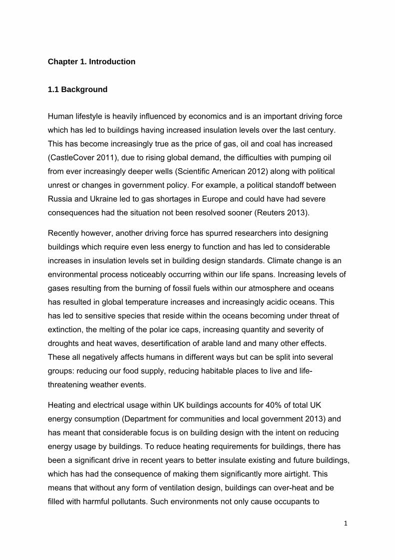
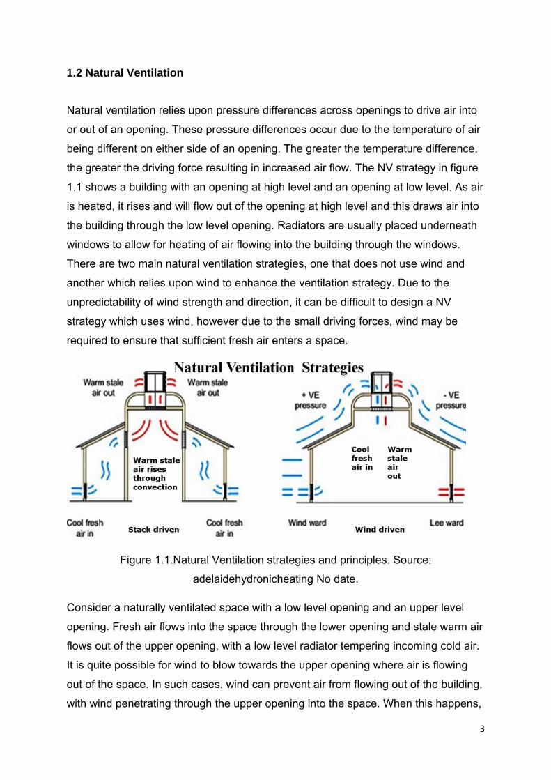
1.2 Natural Ventilation
Natural ventilation relies upon pressure differences across openings to drive air into
or out of an opening. These pressure differences occur due to the temperature of air
being different on either side of an opening. The greater the temperature difference,
the greater the driving force resulting in increased air flow. The NV strategy in figure
1.1 shows a building with an opening at high level and an opening at low level. As air
is heated, it rises and will flow out of the opening at high level and this draws air into
the building through the low level opening. Radiators are usually placed underneath
windows to allow for heating of air flowing into the building through the windows.
There are two main natural ventilation strategies, one that does not use wind and
another which relies upon wind to enhance the ventilation strategy. Due to the
unpredictability of wind strength and direction, it can be difficult to design a NV
strategy which uses wind, however due to the small driving forces, wind may be
required to ensure that sufficient fresh air enters a space.
Figure 1.1.Natural Ventilation strategies and principles. Source:
adelaidehydronicheating No date.
Consider a naturally ventilated space with a low level opening and an upper level
opening. Fresh air flows into the space through the lower opening and stale warm air
flows out of the upper opening, with a low level radiator tempering incoming cold air.
It is quite possible for wind to blow towards the upper opening where air is flowing
out of the space. In such cases, wind can prevent air from flowing out of the building,
with wind penetrating through the upper opening into the space. When this happens,
4
the lower opening which initially had air flowing through it into the space can
experience a flow reversal. This means that air within the space is now flowing past
the radiators directly out to the external environment. With cold external air flowing
into the space at high level the internal temperature can decrease rapidly resulting in
occupants feeling uncomfortable. This problem is exacerbated as internal air flows
past the radiator directly to outside, which renders the radiator ineffective at
providing heat to the space and also increased heating energy used. When such
events occur, the NV strategy is deemed to have failed.
1.3 Water Bath Modelling
WBM is a technique that allows for the simulation of events which has caused a NV
strategy to fail or behave in a way that was not intended. This is because unlike
computational simulations which produce results for only a moment in time,
simulations occur in real time, providing a greater visual understanding of how
airflows develop and form. Chenvidyakarn and Woods (2005) used WBM to show
how wind can fundamentally and permanently change the air flows within a NV
building, leading to substantially different internal temperatures and ventilation rates.
Air flows that vary in time, with no change in driving pressure are deemed to be time-
dependant.
Because the WBM simulations are run in real time, natural variations can be
observed within airflow. These variations are termed transient flows and occur either
due to turbulence within the room or due to some change such as heat source
strength occurring within the building. Monitoring them can vastly improve our
understanding of how NV air flows develop and change with time.
Figure 1.2.shows a WBM simulation, with a model suspended within a large body of
fresh water. Salt water which is dyed blue flows into the model through the top and
because salt water is more dense than fresh water, travels to the bottom of the
model. However, salt water in WBM represents heat in real life scenarios, in effect
meaning that WBM simulations are conducted up-side-down. This simulation has the
floor of the model located at the top of the picture where the salt water flows into the
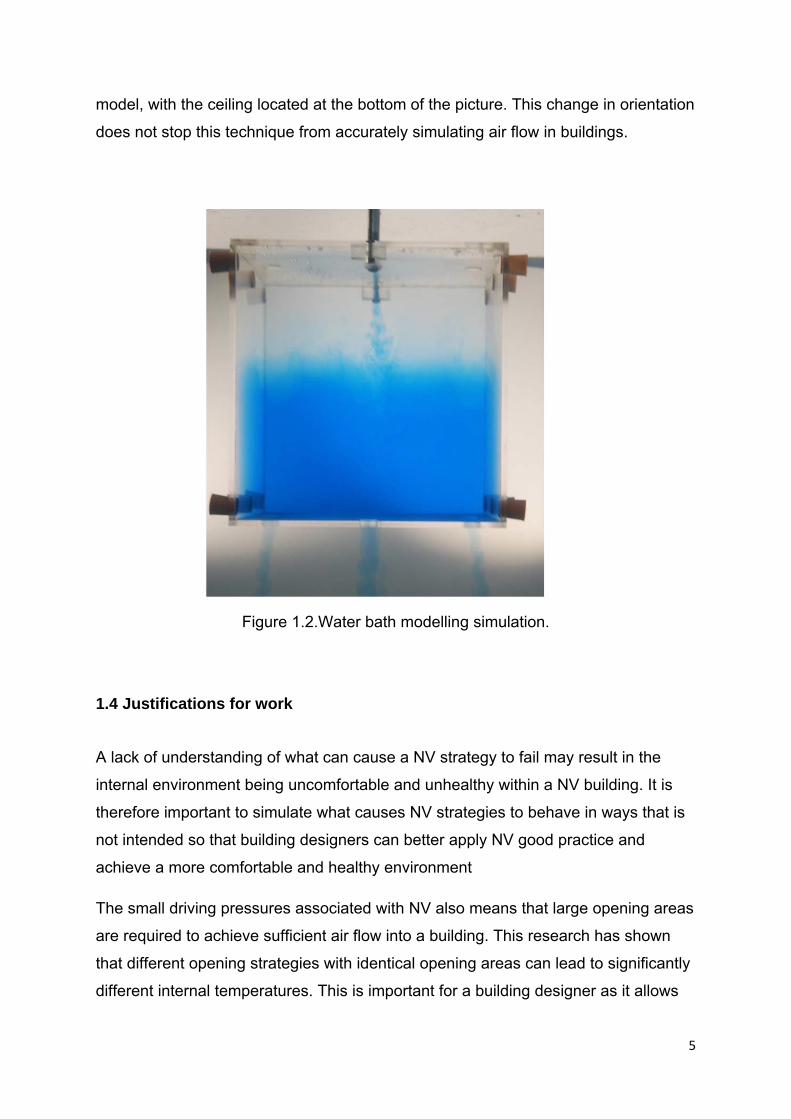
5
model, with the ceiling located at the bottom of the picture. This change in orientation
does not stop this technique from accurately simulating air flow in buildings.
Figure 1.2.Water bath modelling simulation.
1.4 Justifications for work
A lack of understanding of what can cause a NV strategy to fail may result in the
internal environment being uncomfortable and unhealthy within a NV building. It is
therefore important to simulate what causes NV strategies to behave in ways that is
not intended so that building designers can better apply NV good practice and
achieve a more comfortable and healthy environment
The small driving pressures associated with NV also means that large opening areas
are required to achieve sufficient air flow into a building. This research has shown
that different opening strategies with identical opening areas can lead to significantly
different internal temperatures. This is important for a building designer as it allows

6
for a specific NV opening strategy to be selected to achieve certain internal
temperatures which makes the internal environment more comfortable for the
occupants.
Improving our understanding of how to design an efficient and reliable NV strategy
will reduce the need to design buildings with mechanical ventilation or air
conditioning. This will not only save the tenant money with running costs, but also
reduce CO2 emissions resulting in a smaller contribution to global warming.
1.5 Aims and Objectives
This research concentrates on the use of Water Bath Modelling to simulate natural
air flows within reduced scale models of rooms and buildings. The aim of this work is
to better understand the effect that different opening strategies have on internal
temperatures while also analysing transient and time dependant air flows
The objectives of this research are:
‐ Construct a Water Bath Facility (Chapter 2).
‐ Demonstrate agreement between a simple model within the Water Bath using
brine and that of Natural Ventilation theory (Chapter 4).
‐ Compare different opening strategies and their effect on internal temperatures,
interface heights and draining times (Chapter 5).
‐ Force flow regime change and analyse the change in internal temperatures
(Chapter 6).
‐ Simulate a novel ventilation technique with openings at high level for a
hospital ward and analyse the interactions between heat source location and
the rooms geometry (Chapter 7)
7
1.6 Contribution to knowledge
This research has a considerable contribution to ensuring a thermally comfortable space by Natural Ventilation. Such contributions are summarised below:
‐ Chapter 4 o The significantly increased draining times resulting from a small mixed
layer below the interface. o Which theoretical constants to use to accurately predict experimental
results. ‐ Chapter 5
o The resulting internal temperature and flow regime due to different opening strategies and when each strategy is most effective at ensuring a thermally comfortable internal environment.
o Which opening strategies are most effective at ensuring an efficient night purging solution.
‐ Chapter 6 o Manipulating time dependant flow regimes to ensure a Natural
Ventilation Strategy achieves thermal comfort throughout the year. ‐ Chapter 7
o How transient flow interactions between heat source location, opening location and physical geometry of a space can cause significantly different internal temperatures and flow regimes and how to take advantage of such interactions.
8
Chapter 2. Literature Review and Background Theory
2.1 Preamble
This chapter reviews the literature that was used to justify this research and also
presents the context of this work. Principles of Natural Ventilation and the possible
modelling techniques are discussed. The theory behind natural ventilation relating to
the experiments conducted within this research is then presented. Finally, physical
modelling results from previous researchers looking at transient and time dependent
flows in naturally ventilated buildings are discussed. A better understanding of both
of these flows are key features within this research.
2.2 Designing a thermally comfortable and healthy building
In the Middle East, building designs were developed which minimised heat gain,
whilst still allowing daylight into a room. These included the use of bodies of water to
provide cooling, and vegetation to provide shade (Khatami, personal communication
2009). The Romans developed central heating, using a furnace to heat air which was
then circulated around the building (BBC 2011a). For the last few thousand years,
humanity around the world has sought to use building design, technology and
clothing to improve their thermal comfort within their environment. In the past, only
the rich could afford such building designs and technologies, with the majority likely
only having shading to keep cool, or small fires to stay warm. However, with the
introduction of cheap and readily available technology and clothing in the 20th
Century, the rest of the majority of humanity could then similarly improve their
thermal comfort levels.
In modern time, ventilation is used to provide cooling to a space by introducing fresh
air whilst stale warm air flows out of the space. The three main categories of
ventilation are Natural Ventilation (NV), Mechanical Ventilation and air conditioning.
Air conditioning is generally more effective at cooling a space than NV, however
running costs can be considerably more expensive than NV.
Fanger's Predicted Mean Vote (PMV) was developed to quantify comfort in buildings
(Fanger 1970). His equation estimates what percentage of people within a room

9
would likely be thermally comfortable. It is used for building design purposes to
ensure that the thermal environment within a space is acceptable. The equation uses
air temperature, mean radiant temperature (MRT), air velocity and humidity of the
room, along with the metabolic rate and clothing insulation of the people within the
room. Many building standards, including ASHRAE standard 55 (2013), CIBSE
Guide A (2015) and ISO 7730:2005, provide temperature recommendations, based
on Fanger's PMV for the thermal environment of a space. These recommendations
are often a very narrow range of temperatures, and are very difficult to achieve
without some form of Heating, Ventilation and Air Conditioning (HVAC) system. As a
result, many office and school buildings are designed with air conditioning to ensure
a comfortable thermal environment, as predicted by Fanger’s PMV.
The use of air conditioning is increasing around the world, not only in tropical/sub-
tropical areas such as South East Asia (for example Hong Kong and Singapore), but
also in places with a more moderate environment, such as London. In Singapore,
use of air conditioning has increased from 19% of households in 1988, to 58% in
1998 (Wong, Li 2005), with a typical household using 50% of its electricity for air
conditioning (CIBSE Guide F 2012, Low and Cheong 2008). It can be surmised that
as external temperatures continue to rise, more energy will be used to cool down
buildings, and if trends continue, more air conditioning units will come into operation.
However, many field studies have shown that PMV over predicts the thermal
sensation of occupants within a room, often leading to the room being over-cooled,
reducing thermal comfort and wasting energy (Al-ajmi and Loveday 2009, Nicole
2004, Feriadi et al 2003, Busch 1992 and Dear, Leow, and Ameen1991). It has
been suggested that thermal comfort can be achieved in office spaces at much
higher temperatures than what international standards suggest by increasing indoor
air speed (Cho et all 2010 and Candido et al 2008). PMV is even less accurate when
predicting the thermal sensation of occupants within a naturally ventilated building,
especially in hot and humid climates, likely due to behavioural and psychological
adaptations which are not accounted for within the PMV calculation (Brager and
Dear 1998andHumpreys 1978). This suggests that some buildings may be better
suited to implement a natural ventilation strategy, instead of an air conditioning
system. Variants of the PMV model have been implemented to attempt to include the
10
effect of behavioural and psychological adaptations, however they still do not
accurately predict thermal sensation (S. P. Todd 2010).
In light of the inaccuracies that PMV can have when predicting thermal comfort
levels, recent standards have changed internal temperature requirements so that it is
easier for a naturally ventilated building to pass building compliance. For example,
CIBSE Guide A (2006) states that rooms are allowed to have their internal air
temperature to exceed 28°C for 1% of occupied hours per day.
Ventilation is required not only to control the thermal environment within a room, but
also to remove contaminants. Within a space, CO2, Volatile Organic Compounds
(VOCs) such as Formaldehydeand other pollutants can build up, and are linked to
causing Sick Building Syndrome (SBS) and Building Related Illness (BRI) to the
occupants (BRANZ 2007, CIBSE TM40: 2006). The symptoms for SBS and BRI
include headaches, lethargy, skin irritations, fatigue and more (Collet da Graça 2005,
Krogstad et al. 1991). Studies have also shown that excess temperatures, poor
ventilation rates, and poor indoor air quality all reduce the learning ability of students,
along with diminished productivityof office workers (CIBSE Guide A 2007, Kameda
2007, Wargocki 2006, Collet da Graca 2005, Wargocki 2005 Schneider 2002).
Natural ventilation was also shown to be more effective at removing radon gases
than mechanical forms of ventilation in housing (T. Reponen et al 1987).
2.3 Low energy building design
In recent years, substantial evidence has emerged linking the emission of
greenhouse gases (GHG’s) such as carbon dioxide with climate change. These
GHG’s are theorised to contribute to a warming of the earth, causing a 0.4°C rise in
average surface temperature since the 1970s (DECC 2011). Such increases in
temperature, which are not evenly spread across the earth’s surface (Met Office
2009) are thought to be causing the melting of the polar ice caps, rising sea levels,
changing weather patterns and more. It is thought that there will also be an increase
in severe weather events, such as the European heat wave of 2003, which caused
approximately 35,000 deaths throughout Europe (The Stern review 2007). It is also
suggested that the earth faces irreversible damage if temperatures increase beyond

11
2 °C, which is thought to occur if CO2 concentrations increase beyond 400ppm
(Lomas, 2009). In February 2011, CO2 concentrations were measured by the Mauna
Loa Observatory in Hawaii at roughly 391.76 ppm (ESRL, No date).
Buildings are thought to account for 8% of world GHG emissions (Stern review 2007),
whilst 30% of UK GHG emissions are from residential homes, and 20% from
commercial buildings (BBC 2006). In an attempt to reduce CO2 emissions in the
building sector, building regulations are frequently updated to further reduce
associated GHG emissions for new homes. This is achieved by requiring higher
levels of insulation for new buildings and in some cases, the use of renewables such
as photo voltaic (PV). However The Energy Saving trust suggests that a third of new
built homes do not meet the current standards (BBC 2006).
This drive for more sustainable buildings has also looked at ways to reduce our
reliance on energy intensive ventilation systems such as air conditioning and
mechanical ventilation in an attempt to reduce the energy usage of buildings. It is
ironic then, that natural ventilation, a low-energy form of building ventilation which
has been used since buildings were first built, is being encouraged again. The cost
savings of running a naturally ventilated building can be quite substantial compared
to an air conditioned building, with NV buildings typically using 40% or less energy
compared to AC buildings (Energy Consumption Guide 19 1993). The cost of
constructing an AC building may also be substantially more than a NV building due
to costs of air conditioning plant, although this may not always be the case if
advanced facades and other expensive features are used in the NV building design.
2.4 Natural ventilation
Natural ventilation (NV) is a ventilation strategy which relies on temperature
differences or wind to drive a flow of fresh air into a space (Figure 2.1). As air is
heated, it becomes less dense and rises, ultimately flowing out of an opening at high
level. This draws air into the space from another opening usually at a lower level to
replace air which is leaving the space. NV strategies may attempt to minimise the
effect of wind to allow for greater ventilation control or manipulate the effect of wind
to increase the ventilation of a space. Designers often attempt to mitigate the chance
12
of wind interacting with a natural ventilation strategy of a building due to its
unpredictability (with both strength and direction) and also because it is generally a
‘stronger’ force than the driving forces generated from temperature differences which
occur within a NV strategy. Where the force of wind aids or counteracts the NV
buoyancy forces, an increase or decrease in ventilation rate will likely occur which
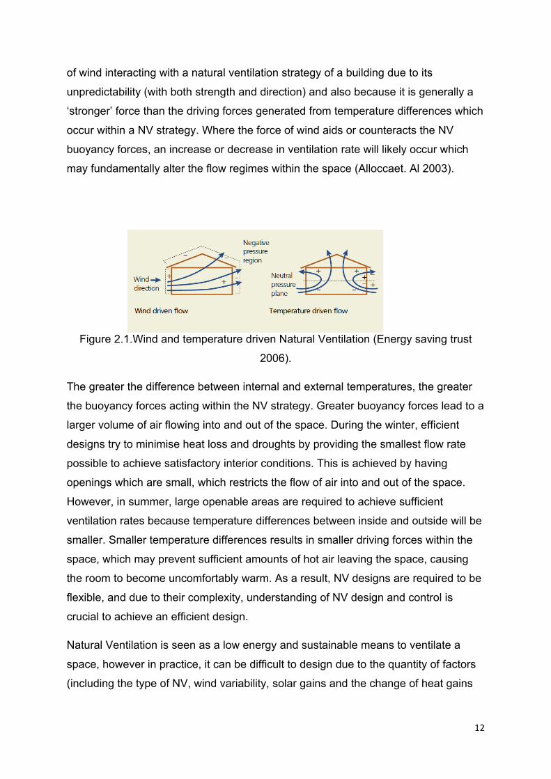
may fundamentally alter the flow regimes within the space (Alloccaet. Al 2003).
Figure 2.1.Wind and temperature driven Natural Ventilation (Energy saving trust
2006).
The greater the difference between internal and external temperatures, the greater
the buoyancy forces acting within the NV strategy. Greater buoyancy forces lead to a
larger volume of air flowing into and out of the space. During the winter, efficient
designs try to minimise heat loss and droughts by providing the smallest flow rate
possible to achieve satisfactory interior conditions. This is achieved by having
openings which are small, which restricts the flow of air into and out of the space.
However, in summer, large openable areas are required to achieve sufficient
ventilation rates because temperature differences between inside and outside will be
smaller. Smaller temperature differences results in smaller driving forces within the
space, which may prevent sufficient amounts of hot air leaving the space, causing
the room to become uncomfortably warm. As a result, NV designs are required to be
flexible, and due to their complexity, understanding of NV design and control is
crucial to achieve an efficient design.
Natural Ventilation is seen as a low energy and sustainable means to ventilate a
space, however in practice, it can be difficult to design due to the quantity of factors
(including the type of NV, wind variability, solar gains and the change of heat gains
13
strength and location)which affect the flow rate (Collet da Graça 2005, Allocca2003),
and offers limited control to the occupants compared to other ventilation strategies.
Due to the small driving forces involved in a temperature-driven NV strategy, low
flow rates can result. This means that there may have to be very large opening areas
to ensure sufficient ventilation, especially when internal and external temperature
differences are quite small. Such large opening areas can be difficult to achieve due
to the geometry of the room and building and are difficult to control, which may lead
to significant energy losses and droughts which will reduce thermal comfort during
the winter (Becker et al. 2006). The placement of these openings is also important,
not only affecting the effectiveness of the ventilation strategy (Mumovicet al. 2009,
Janssen et al. 1982), but also leading to potential problems of outside noise and air
pollution. If relatively small driving forces are achieved within an NV strategy, it is
likely that insufficient ventilation will occur with a certain design. In such cases, the
design of the building may attempt to incorporate wind where possible, by using
technologies such as ‘wind towers’, which are designed to allow wind to flow into a
space, therefore increasing ventilation rates (Hughes and Cheuk-ming 2011, Khan et
al 2008). However, such designs which rely on wind may struggle during warm
summers where less wind occurs, and as a result, buildings may have to incorporate
extra opening windows or low powered fans to increase air flow (Lomas 2007).
Because a building shell can last for 60 years (Bordasset al 1996), along with the
likelihood of increased external temperatures in the future due to global warming, NV
strategies need to be designed to be resilient to changes in weather conditions. They
must also take into consideration that the usage of the space may change with time,
resulting in varying ventilation requirements. Such long term conditions can further
complicate the ability to provide a suitable NV strategy, which demonstrates the
importance of this research.
A low energy building design which uses NV will likely be more expensive to build
than a cheap ‘no frills’ alternative, but it is likely that the increased construction costs
will be recouped by lower running costs, along with improving occupant satisfaction
and productivity (Akimoto 2009, CIBSE Guide A 2007, Wagner et al. 2007, and
Menzies et al 2004). For example, Facebook’s new data centre uses 38% less
14
power than existing data centres, where much of the savings are said to have come
from replacing air conditioning units with a form of natural ventilation (BBC 2011b).
2.5 Simulating Natural Ventilation
During the design phase of a yet to be constructed building, simulations are
undertaken to assess the effectiveness of proposed ventilation systems. These
simulations may provide estimates of indoor temperatures, thermal stratification and
flow rates through openings allowing for an indication as to whether a NV design
allows for a space to achieve internal temperature and ventilation rates dictated by
the client and building regulations. There are three main types of simulation
techniques, analytical, experimental and computer simulations.
Analytical models are often employed at very early stages of design. These involve a
small number of simple equations. Such models can provide results which are
applicable to just one moment in time (Andersen 2004, Hunt and Linden 2004, Li
2000). It has been suggested that the applicability of analytical equations is limited
(Allocca et al 2003) because they do not take account of the form of the building
design, the building surroundings, along with the interior space and any other
complexities (Jiang and Chen 2003, Gangoiti et al. 1997). However these equations
are easy to compute and apply, and can be used to determine the required opening
areas that should be used when looking at initial designs (Lomas 2007). It should
also be noted that there has been close agreement between empirical modelling with
Computational Fluid Dynamics (CFD) simulations (Allocca 2003), wind tunnel testing
(Andersen 2007) and water bath modelling (Linden et al 1990) when looking at
simple cases.
There are two main types of computer simulations: zonal/network and CFD. Zonal
and network air flow simulations simulate a building over a period of time, varying
conditions including weather, heating & cooling, and occupancy (Adamu et al. 2011).
Such programmes are used to check for compliance with temperature, indoor air
quality and ventilation rates with building regulations. However, data is provided in
intervals, perhaps every 15 minutes, and assumes that the air within each room is
15
well mixed. Computational Fluid Dynamics (CFD) uses a very large number of
equations to iteratively solve a steady state (in some cases transient simulations can
be achieved if sufficient computing resource is available) solution and requires the
user to choose many boundary conditions, mathematical models and assumptions.
CFD simulations can generally only simulate a moment in time, but is however, able
to provide a large amount of precise information, including temperature, air speed
and humidity at any position within the room.
Physical modelling techniques involve the construction of scaled models. There are
two main types of physical modelling techniques; those that use air as a working
medium, and those that use water. When using air as the working medium, flow
patterns of the air within the model are observed by using smoke, with pressures on
facades due to wind, along with the effect of wind on flow patterns within the room
generally being simulated (Zhen Bu et al 2010, Andrew et al 2009, Karava et al 2007,
Walker 2005, Yi Jiang and Chen 2003). A heat source is simulated within the room
by using a heater. Water based simulations known as water bath modelling will
either use heaters, or use a fluid of a density different from that of the fresh water to
simulate a heat source within the model. Often, brine (water with dissolved salt in
concentrations up to 20%) is used to simulate air which has been heated by a heat
source within the room. This is achieved by brine flowing into the model at the
location where a heat source would be. The density differences between water and
brine allow for conversions into temperature differences in air. Water bath modelling
using brine is explained in detail in chapter 3.
Experimental techniques do not provide as much information as computer
simulations, however, they allow for visualisation of the flow as it develops. This is
important as it helps better understand the transient development of flows and how
ventilation systems react to changes within the space. Such changes could involve a
change in heat source strength/location or wind blowing through an opening and can
cause fundamental changes to the thermal environment within the space. If a
temporary change (for example a gust of wind) causes a permanent change in the
thermal environment within the space, then the flow is described as time dependent.
Such flows can result in disastrous consequences for the thermal environment within
a space, resulting in occupants being thermally uncomfortable whilst also increasing
energy consumption during winter heating.

16
2.6 Principles of buoyancy driven natural ventilation
Consider the forces of gravity and buoyancy acting upon a volume of air (Figure 2.2).
If there is no initial velocity in any direction acting upon the volume of air, then gravity
and buoyancy will determine if the air rises, falls, or remains at the same height. The
forces of gravity, along with the mass of the volume of air, are constants, however
the buoyancy of the air will change depending on the density of the air, and the
density of the fluid around the air.
Figure 2.2. Principle forces acting upon a volume of air.
If the temperature of the volume of air is increased, then its density decreases. If the
air's density decreases, its buoyancy increases. The increase in buoyancy means
that the air will rise if the surrounding fluid has a lower buoyancy. Conversely, if the
air cools down, its density increases, and therefore its buoyancy decreases.
Natural ventilation strategies are usually designed to take advantage of this
buoyancy force within the space, to drive flow out of the room, drawing in fresh air
from the inlet. The greater the temperature difference within the room, the greater
the buoyancy force within the space, meaning that more fresh air will be driven into
and stale air out of the space.
Buoyancy
Gravity

17
Figure 2.3 illustrates a simple displacement NV strategy (Linden et al 1990). A low
level opening allows cool outside air to enter and a high outlet allows hot air to exit.
Displacement ventilation forms a warmer than ambient stratified layer at a height ‘h’
above the heat source, with ambient temperature below the stratified layer. H is the
height difference between the inlet, and the outlet, for this case with vertical
openings, the midpoint in height of each opening is used. A plume of warm air rises
above the heat source and as it rises, turbulent mixing between the plume and the
ambient fluid around the plume causes the plume to increase in width as it rises.
This process is referred to as “entrainment” and will be discussed in section 2.7.2.1.
The air within the plume below the stratified layer rises due to it having a lower
density than the ambient air around the plume. However, when the plume passes
through the stratified layer, the particles from the plume continue to rise even though
the density above the stratified layer and that of the plume is similar. This can be
attributed to the upward momentum that the particles gained due to buoyancy
differences while below the stratified layer.
Figure 2.3.Principles of buoyancy-driven Natural Ventilation with a single heat source.
Displacement NV strategies are designed to keep the stratified layer at a height
above the occupants to ensure that the occupants are thermally comfortable.
Importantly, the concentration of contaminants within a space using displacement
ventilation is at its greatest within the stratified layer, so if the stratified layer was at a
low height, the occupants may be exposed to ‘dirty air’ (Bolster and Linden 2007).
Lower
opening
Upper
opening
Heat source
Stratified
layer
h
H

18
Figure 2.4 shows the main strategies for natural ventilation. A single opening
strategy means that a single window, door or other opening with access to fresh air
will have air flowing into and out of it at the same time. Single sided NV is generally
employed in small rooms (where the depth of the room is less than 2.5H) with low
heat gains, with air flowing both into and out of the room through the single opening.
However, during summer, small buildings may have to rely upon wind to drive the
flow due to small temperature difference between internal and external air (Khan et
al 2008). A cross ventilation strategy uses two or more openings on opposite sides of
the room. Some of the openings will be designed to be inlets, which will allow fresh
air into the room, while other openings will be outlets, allowing warm and polluted air
to leave the room. Cross ventilation is used for larger rooms with increased heat gain,
but when there is very large heat gains, a stack ventilation strategy will be used to
further increase the flow rate within a room. Stack ventilation strategies increase the
height difference between lower and upper openings, resulting in increased flow rate
through the building.
a) b) c)
Figure 2.4.Basic Natural Ventilation Strategies: a) Single opening, b) cross
ventilation and c) stack natural ventilation.
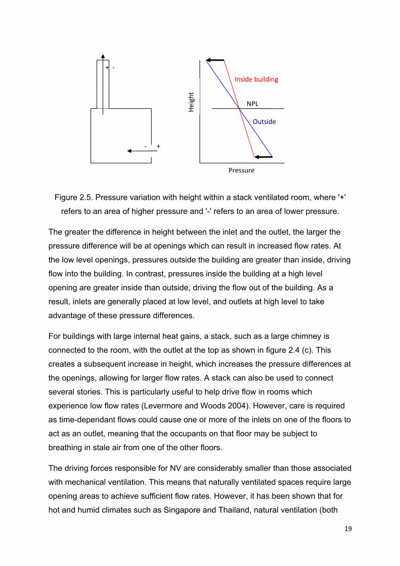
The pressure difference across an opening is a force that draws air through an
opening. This pressure difference varies with height, but is equal to zero at some
height known as the Neutral Pressure Level (NPL), between the inlets and outlets,
and increases with distance from this point (Figure 2.5). Any openings close to the
NPL will experience little or no air flow into or out of the space due to the lack of any
pressure difference.
H H
19
Figure 2.5. Pressure variation with height within a stack ventilated room, where '+'
refers to an area of higher pressure and '-' refers to an area of lower pressure.
The greater the difference in height between the inlet and the outlet, the larger the
pressure difference will be at openings which can result in increased flow rates. At
the low level openings, pressures outside the building are greater than inside, driving
flow into the building. In contrast, pressures inside the building at a high level
opening are greater inside than outside, driving the flow out of the building. As a
result, inlets are generally placed at low level, and outlets at high level to take
advantage of these pressure differences.
For buildings with large internal heat gains, a stack, such as a large chimney is
connected to the room, with the outlet at the top as shown in figure 2.4 (c). This
creates a subsequent increase in height, which increases the pressure differences at
the openings, allowing for larger flow rates. A stack can also be used to connect
several stories. This is particularly useful to help drive flow in rooms which
experience low flow rates (Levermore and Woods 2004). However, care is required
as time-dependant flows could cause one or more of the inlets on one of the floors to
act as an outlet, meaning that the occupants on that floor may be subject to
breathing in stale air from one of the other floors.
The driving forces responsible for NV are considerably smaller than those associated
with mechanical ventilation. This means that naturally ventilated spaces require large
opening areas to achieve sufficient flow rates. However, it has been shown that for
hot and humid climates such as Singapore and Thailand, natural ventilation (both
Pressure
Height
NPL
Inside building
Outside
‐ +
+ ‐

20
stack and cross) can provide sufficient ventilation rates to allow for appropriate levels
of thermal comfort for domestic applications (Prajongsan and Sharples 2012,
Stephen Todd 2010, R. Priyadarsini et al 2004, Tantasavasdi 2001). As a result, in
more temperate climates such as western Europe and Northern America, natural
ventilation strategies can also be applied.
2.7 Analytical Models for Natural Ventilation and Plume Theory
2.7.1 Emptying space with no continuous heat source
Linden et al (1990) produced an analytical model which described a room which is
initially filled with warmer than ambient air, with no heat source and with inlet and
outlet openings. Such a scenario could occur when people leave a room, or when a
night cooling strategy is being used (Figure 2.6). The theory and resulting equations
in this section are taken from Linden et al (1990) unless otherwise stated.
Figure 2.6. Emptying space, initially filled with warmer than ambient air based on a
night purging strategy.
The interface height is the height at which a separation between warmer than
ambient air and ambient air occurs (Figure 2.6).H is the height between inlet and
outlet, h is the height of the interface measured from the inlet, z is the distance
between the interface height and the NPL and u represents the flow rate of air
through an opening. Because there is no heat source, the interface height, h, will
increase as the warmer than ambient air leaves through the top opening. As hot air
leaves through the outlet, cool ambient air is drawn in through the inlet.
NPL H
u2(lower opening)
u1 (upper opening)
z
h

21
The flow rates, u, through high level and low level openings are given by equation
2.1 and 2.2 respectively:
2.1
2.2
where Cd is the coefficient of discharge, describing the expansion of the fluid going
through the opening, and is equal to 0.5 for sharp expansion at the inlet and 1 for a
perfectly smooth expansion. g’ is the reduced gravity, which is a simple way to
represent buoyancy.
The flow rate through a space can also be calculated using equation 2.3 (Etheridge
and Sandberg 1996).
q C A 2∆P/ϱ 2.3
where∆p is the pressure difference across an opening calculated by equation 2.4.
∆P ∆ϱgH 2.4
Equation 2.3 assumes that if the openings are on a vertical plane, they are
sufficiently small in height that there is only a small pressure difference along the
vertical axis across the height of the opening. When the openings are sufficiently
large enough such that the pressure drops across the vertical plane, this should be
taken into account using work provided by Li et al (2000).
By increasing the temperature of a particle, its density decreases causing the particle
to increase in altitude. To describe the change in buoyancy of a particle when its
temperature changes, equation 2.5 is used which calculates the reduced gravity, g'.
Calculating the reduced gravity of a particle assumes that as the temperature
changes, the density remains constant and instead the force of gravity acting upon
the particle changes. For example, a particle gains energy, resulting in an increase in
temperature causing the particle to rise. Equation 2.5 assumes that the force of
gravity reduced to allow the particle to rise, becoming more buoyant as a result.
2.5
dzCgu
zhHgu
'22
'21
2
)(2
T
Tggg
'
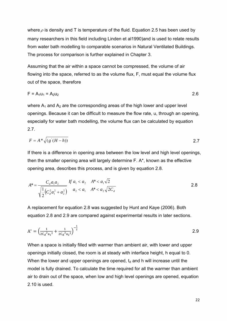
22
where is density and T is temperature of the fluid. Equation 2.5 has been used by
many researchers in this field including Linden et al1990)and is used to relate results
from water bath modelling to comparable scenarios in Natural Ventilated Buildings.
The process for comparison is further explained in Chapter 3.
Assuming that the air within a space cannot be compressed, the volume of air
flowing into the space, referred to as the volume flux, F, must equal the volume flux
out of the space, therefore
F = A1u1 = A2u2 2.6
where A1 and A2 are the corresponding areas of the high lower and upper level
openings. Because it can be difficult to measure the flow rate, u, through an opening,
especially for water bath modelling, the volume flux can be calculated by equation
2.7.
2.7
If there is a difference in opening area between the low level and high level openings,
then the smaller opening area will largely determine F. A*, known as the effective
opening area, describes this process, and is given by equation 2.8.
22
21
2
21
2
1*
aaC
aaCA
d
d
dCaAaa
aAaaIf
2*
2*
212
121
2.8
A replacement for equation 2.8 was suggested by Hunt and Kaye (2006). Both
equation 2.8 and 2.9 are compared against experimental results in later sections.
A∗ 2.9
When a space is initially filled with warmer than ambient air, with lower and upper
openings initially closed, the room is at steady with interface height, h equal to 0.
When the lower and upper openings are opened, td and h will increase until the
model is fully drained. To calculate the time required for all the warmer than ambient
air to drain out of the space, when low and high level openings are opened, equation
2.10 is used.
))((* ' hHgAF
23
2
11
et
t
H
h 2.10
where te is the time that it would take for the space to empty, given by:
'*
2
g
H
A
Ste
2.11
where S is the floor area of the space. If the interface height is at some height other
than 0, the room can be considered to have been draining for some time. Equation
2.12 calculates the amount of time draining has been occurring for the interface to
reach that height.
2
11
e
t
t
t
H
h 2.12
where ht is the interface height at time t.
The theory presented so far has been for classical displacement draining flows,
which involves an interface height steadily increasing in height as hot air flows out of
the outlets. Hunt and Coffey (2010) showed that there can be four possible flow
regimes for a space which can occur when a space is draining including classical
displacement flow which they term as flow regime 1(Figure 2.7).
To show the four different draining flow regimes, Hunt and Coffey (2010) conducted
experiments in a water bath, simulating the scenario where the room is initially filled
with warmer than ambient air, upper openings are initially closed and with no heat
source. The model used was a simple box with openings on the floor and ceiling of
the model. Certain openings placed on the ceiling were then opened. Hunt and
Coffey (2010) then showed how the flow within the space varied depending on the
ratio between the opening areas of the lower and upper openings, R, along with the
ratio between interface height and the height of the room,ξ0.

24
1 2 3 4
Figure 2.7. Four possible flow regimes for an emptying space. Source: Hunt and
Coffey (2010).
For flow regime 2, fluid was observed to flow through the lower openings such that it
penetrates the interface and mixes with the initially uniform warmer than ambient
fluid above the interface causing a three layer stratification (Figure 2.8). The top
layer has the same temperature as the layer above the interface at initial starting
conditions. The middle layer has a temperature which is less than that of the top
layer but is greater than ambient. This layer increases in size vertically upwards and
downwards until it fills the entire space and the top layer has entirely vented through
the outlet. At this point, the space is fully mixed and the temperature decreases until
ambient temperature is reached.
1
ξ0
0 1/4
R

25
a) t=0s b) t=15s c) t= 60s d) t= 120s
Figure 2.8.Images of a space emptying with flow regime 2. Figure a), b), c) and d)
show draining at times 0, 15, 60 and 120 seconds consecutively where time to empty,
te = 375s. Source: Hunt and Coffey (2010).
Flow regimes 3 (Figure 2.9) and 4 (Figure 2.10) involve bi-directional flow through
the upper opening because the opening area of the lower opening is considerably
smaller than the upper opening. Such bi-directional flows occur when the upper
opening area, a2> 4a1. Perhaps the most important observation between the four
flow patterns is that the ones with bi-directional flow take considerably longer to drain
than those with mono-directional flow through the openings.
Except for the observed bi-directional flow, flow regime 3 is similar to flow regime 2
while flow regime 4 can be described as a very slow draining version of flow regime
1.
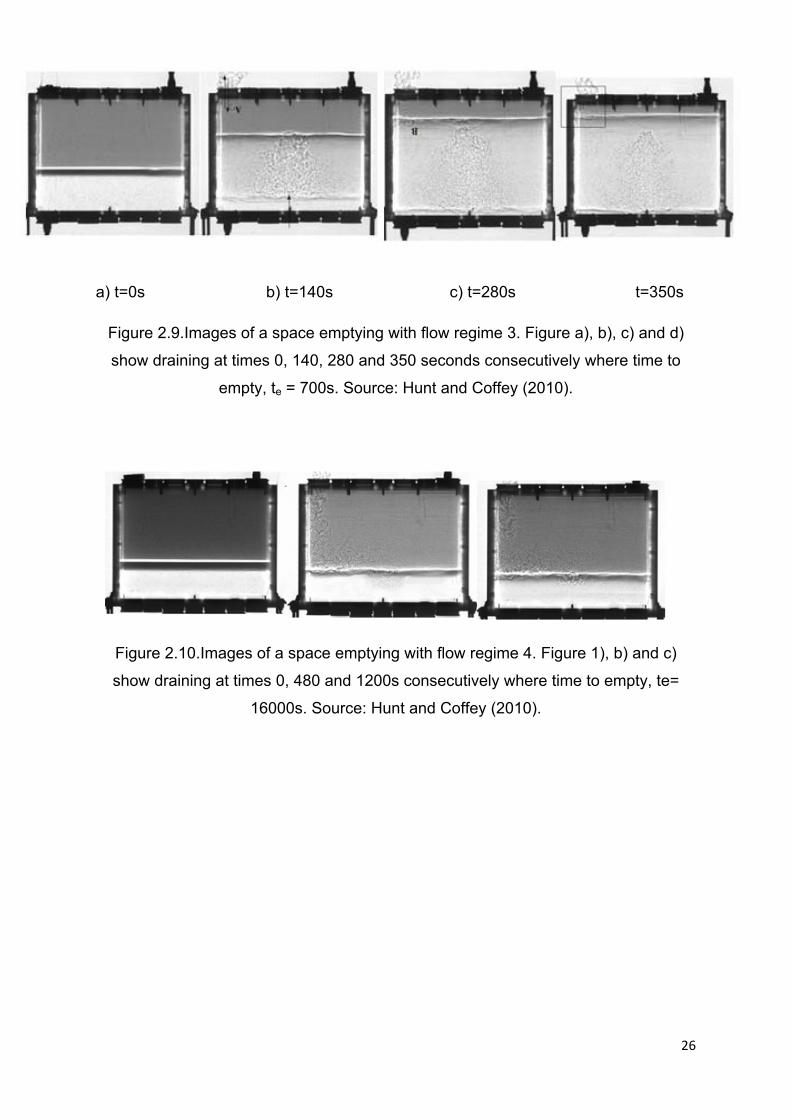
26
a) t=0s b) t=140s c) t=280s t=350s
Figure 2.9.Images of a space emptying with flow regime 3. Figure a), b), c) and d)
show draining at times 0, 140, 280 and 350 seconds consecutively where time to
empty, te = 700s. Source: Hunt and Coffey (2010).
Figure 2.10.Images of a space emptying with flow regime 4. Figure 1), b) and c)
show draining at times 0, 480 and 1200s consecutively where time to empty, te=
16000s. Source: Hunt and Coffey (2010).
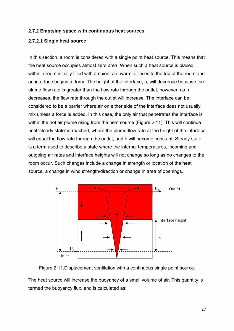
27
2.7.2 Emptying space with continuous heat sources
2.7.2.1 Single heat source
In this section, a room is considered with a single point heat source. This means that
the heat source occupies almost zero area. When such a heat source is placed
within a room initially filled with ambient air, warm air rises to the top of the room and
an interface begins to form. The height of the interface, h, will decrease because the
plume flow rate is greater than the flow rate through the outlet, however, as h
decreases, the flow rate through the outlet will increase. The interface can be
considered to be a barrier where air on either side of the interface does not usually
mix unless a force is added. In this case, the only air that penetrates the interface is
within the hot air plume rising from the heat source (Figure 2.11). This will continue
until ‘steady state’ is reached, where the plume flow rate at the height of the interface
will equal the flow rate through the outlet, and h will become constant. Steady state
is a term used to describe a state where the internal temperatures, incoming and
outgoing air rates and interface heights will not change so long as no changes to the
room occur. Such changes include a change in strength or location of the heat
source, a change in wind strength/direction or change in area of openings.
Figure 2.11.Displacement ventilation with a continuous single point source.
The heat source will increase the buoyancy of a small volume of air. This quantity is
termed the buoyancy flux, and is calculated as:
H
U2
U1
h
Interface height
Outlet
Inlet
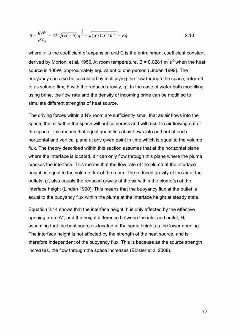
28
'/)/'(')(*' 532
3
FghCgghHAc
WgB
p
2.13
where is the coefficient of expansion and C is the entrainment coefficient constant
derived by Morton, et al. 1956. At room temperature, B = 0.0281 m4s-3 when the heat
source is 100W, approximately equivalent to one person (Linden 1999). The
buoyancy can also be calculated by multiplying the flow through the space, referred
to as volume flux, F with the reduced gravity, g’. In the case of water bath modelling
using brine, the flow rate and the density of incoming brine can be modified to
simulate different strengths of heat source.
The driving forces within a NV room are sufficiently small that as air flows into the
space, the air within the space will not compress and will result in air flowing out of
the space. This means that equal quantities of air flows into and out of each
horizontal and vertical plane at any given point in time which is equal to the volume
flux. The theory described within this section assumes that at the horizontal plane
where the interface is located, air can only flow through this plane where the plume
crosses the interface. This means that the flow rate of the plume at the interface
height, is equal to the volume flux of the room. The reduced gravity of the air at the
outlets, g’, also equals the reduced gravity of the air within the plume(s) at the
interface height (Linden 1990). This means that the buoyancy flux at the outlet is
equal to the buoyancy flux within the plume at the interface height at steady state.
Equation 2.14 shows that the interface height, h is only affected by the effective
opening area, A*, and the height difference between the inlet and outlet, H,
assuming that the heat source is located at the same height as the lower opening.
The interface height is not affected by the strength of the heat source, and is
therefore independent of the buoyancy flux. This is because as the source strength
increases, the flow through the space increases (Bolster et al 2008).
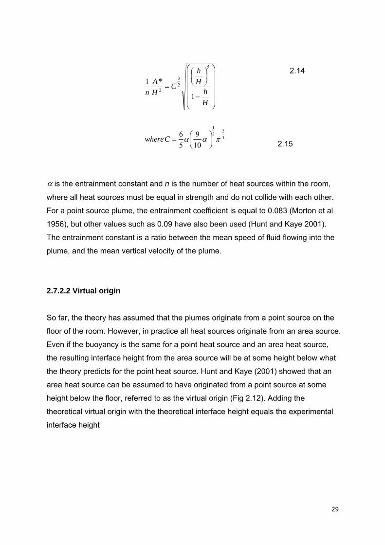
29
2.14
2.15
is the entrainment constant and n is the number of heat sources within the room,
where all heat sources must be equal in strength and do not collide with each other.
For a point source plume, the entrainment coefficient is equal to 0.083 (Morton et al
1956), but other values such as 0.09 have also been used (Hunt and Kaye 2001).
The entrainment constant is a ratio between the mean speed of fluid flowing into the
plume, and the mean vertical velocity of the plume.
2.7.2.2 Virtual origin
So far, the theory has assumed that the plumes originate from a point source on the
floor of the room. However, in practice all heat sources originate from an area source.
Even if the buoyancy is the same for a point heat source and an area heat source,
the resulting interface height from the area source will be at some height below what
the theory predicts for the point heat source. Hunt and Kaye (2001) showed that an
area heat source can be assumed to have originated from a point source at some
height below the floor, referred to as the virtual origin (Fig 2.12). Adding the
theoretical virtual origin with the theoretical interface height equals the experimental
interface height
3
23
1
5
2
3
2
10
9
5
6
1
*1
Cwhere
H
hH
h
CH
A
n

30
.
Figure 2.12.Virtual origin of a heat source.
Hunt and Kaye (2001) showed how to calculate the virtual origin for a plume. Their
method takes into account the source conditions of the plume, including flow rate,
buoyancy and momentum. To calculate the asymptotic virtual origin, z*avs, the
following method can be employed. The initial buoyancy flux of the plume, Bf is
calculated by multiplying the volume flux, F with the reduced gravity, g’ as shown in
equation 2.16.
Bf = Fg’ 2.16
Then the momentum flux of the plume, m is calculated:
m = F2 / A 2.17
where An is the nozzle area (cm2). The momentum jet length, Lm is given by:
2
1
4
3
4
1
2
1
4
5
2
f
m
B
mL
2.18
and the source flow rate length, La:
2
12
112
31 523
B
FLa
2.19
Hot air plume
rising
Heat source
Ground
Virtual origin location of
the ‘point source’ of the
heat source
z
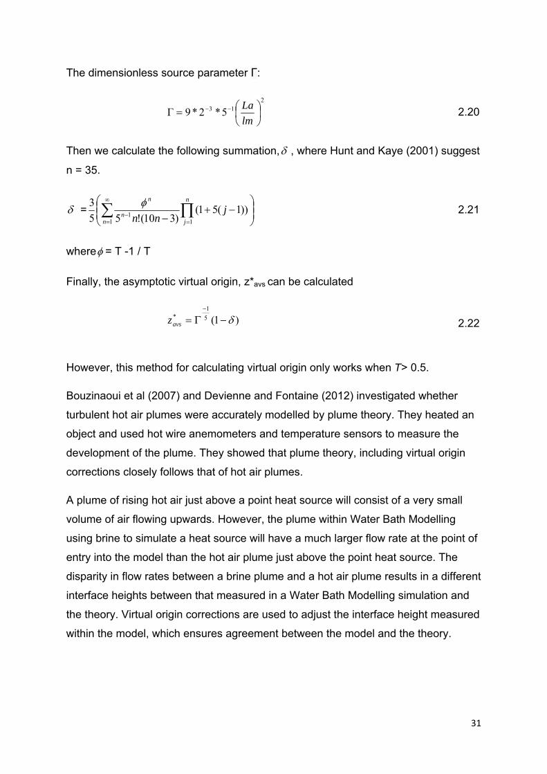
31
The dimensionless source parameter Γ:
213 5*2*9Γ
lm
La 2.20
Then we calculate the following summation, , where Hunt and Kaye (2001) suggest
n = 35.
=
1 11
))1(51()310(!55
3
n
n
jn
n
jnn
2.21
where = T -1 / T
Finally, the asymptotic virtual origin, z*avs can be calculated
)1(5
1*
avsz 2.22
However, this method for calculating virtual origin only works when T> 0.5.
Bouzinaoui et al (2007) and Devienne and Fontaine (2012) investigated whether
turbulent hot air plumes were accurately modelled by plume theory. They heated an
object and used hot wire anemometers and temperature sensors to measure the
development of the plume. They showed that plume theory, including virtual origin
corrections closely follows that of hot air plumes.
A plume of rising hot air just above a point heat source will consist of a very small
volume of air flowing upwards. However, the plume within Water Bath Modelling
using brine to simulate a heat source will have a much larger flow rate at the point of
entry into the model than the hot air plume just above the point heat source. The
disparity in flow rates between a brine plume and a hot air plume results in a different
interface heights between that measured in a Water Bath Modelling simulation and
the theory. Virtual origin corrections are used to adjust the interface height measured
within the model, which ensures agreement between the model and the theory.
32
2.7.2.3 Two heat sources within a room which do not interact
Cooper and Linden (1996) showed that for the case where there are two or more
identical heat sources sufficiently separated so that the plumes rising above the heat
sources do not collide, then the interface height will be the same as if there was just
one of those heat sources within the space.
When two or more sources within a room have different source strengths, multiple
interfaces form. For the case in figure 2.13, P1 represents a plume which is less
buoyant than plume P2. As a result, a plume of warm air rises above both heat
sources, and entrainment occurs as normal. Because there are two heat sources of
different source strengths, two interfaces form (Figure 2.13).
Both plumes pass through interface A. As a result, adding both volume fluxes of the
plumes at the interface height A equals the total volume flux through the space. The
lower region of warm air above interface A is caused by a build-up of warmer than
ambient air from plume 1, of temperature T1. The plume P2 will be less dense than
P2. As a result, P2 penetrates the first warm layer and forms another layer of warmer
than ambient air, at temperature T2, where T2 > T1. P2 entrains warm air from the
lower warm air region and passes through interface B with volume flux F. As a result,
when a steady state is reached, the difference in volume flux, F, for P1 at interface A
and interface B is equal to the volume flux of P2 at interface A.
33
Figure 2.13.Displacement ventilation with two heat sources of different strengths.
The analytical models for volume flux through the space (2.23) and the interface
heights (2.24) derived by Cooper and Linden (1996) closely agreed with their water
bath simulations.
))()((* 12'12
'2 hhghHgAF 2.23
H
hh
B
B
B
B
H
h
H
h
B
B
B
B
CH
A
12
2
1
3
2
2
1
1
5
2
1
2
3
3
2
1
2
32
1
1
1
1
1*
2.24
P2P1
U2
U1
h
Interface A
Outlet
Inlet
Interface B
T1
T2
h2
h1
g2’
g1’
H
34
2.7.2.4 Interacting turbulent plumes with identical buoyancies
Kaye and linden (2004) investigated the case of two identical plumes, with their
sources horizontally separated at a distance, Xo which was sufficiently close to allow
for the plumes to collide and coalesce at some height. They showed that the height
at which the two plumes of equal buoyancy merge (height Zm) is equal to 4.8χ0,
where χ0 is the initial separation between the two plumes. If the plumes do not have
the same buoyancy, Zm decreases as the difference in buoyancy between the two
plumes decreases.
At the point where two equal plumes combine, the resulting plume can be
considered to be a single plume. The virtual origin of this plume is calculated in the
same way as a normal point source plume (see section 2.7.2.2). As a result, the
virtual origin will be 1.37 plume separations below the two original plumes (Figure
2.14).
Kaye and Linden (2004) observed in their water bath experiments that when two
equal plumes converged, the resulting plume stopped entraining for a brief period of
time and therefore had vertical sides, before entrainment continued.
They surmised that the resulting plume had a Γ value greater than 1 (therefore lazy),
and the plume edges remained vertical while Γ of the plume decreased to 1 (pure
plume), before entrainment continued. As a result, Kaye and Hunt (2004) surmised
that when using brine plumes, it is better for Γ at the source to be as close to 1 as
possible.
35
Figure 2.14.The merging of two identical plumes separated by some distance
Xo.Source: Kaye and linden 2004.
The flow rate and momentum flux of the merged plume is given by equation 2.25:
3
5
03
1
5
6
4
52
F
Q 2.25
3
4
03
2
5
6
4
52
F
M 2.26
Where o
z
2.27
The buoyancy fluxof the merged plume is equal to the sum of the two buoyancy flux
of the plumes before merging.
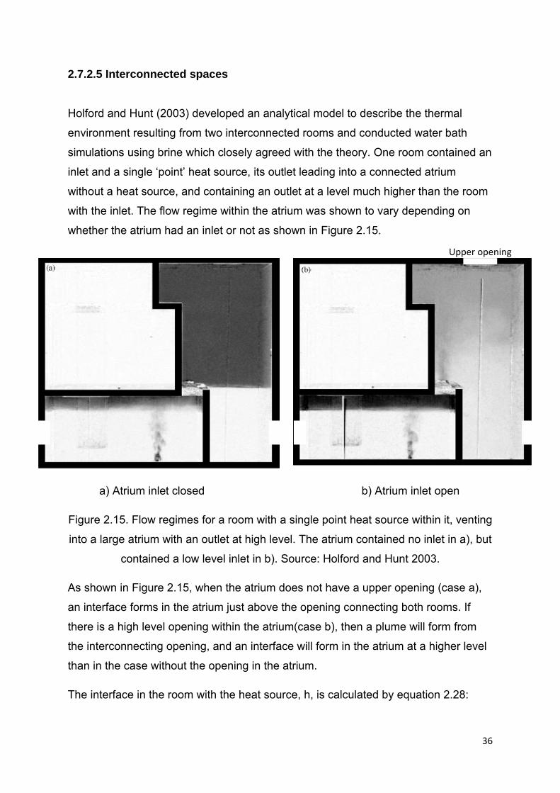
36
2.7.2.5 Interconnected spaces
Holford and Hunt (2003) developed an analytical model to describe the thermal
environment resulting from two interconnected rooms and conducted water bath
simulations using brine which closely agreed with the theory. One room contained an
inlet and a single ‘point’ heat source, its outlet leading into a connected atrium
without a heat source, and containing an outlet at a level much higher than the room
with the inlet. The flow regime within the atrium was shown to vary depending on
whether the atrium had an inlet or not as shown in Figure 2.15.
a) Atrium inlet closed b) Atrium inlet open
Figure 2.15. Flow regimes for a room with a single point heat source within it, venting
into a large atrium with an outlet at high level. The atrium contained no inlet in a), but
contained a low level inlet in b). Source: Holford and Hunt 2003.
As shown in Figure 2.15, when the atrium does not have a upper opening (case a),
an interface forms in the atrium just above the opening connecting both rooms. If
there is a high level opening within the atrium(case b), then a plume will form from
the interconnecting opening, and an interface will form in the atrium at a higher level
than in the case without the opening in the atrium.
The interface in the room with the heat source, h, is calculated by equation 2.28:
Upper opening
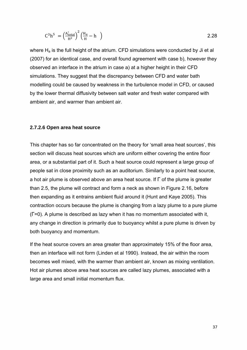
37
C h∗
h 2.28
where Ha is the full height of the atrium. CFD simulations were conducted by Ji et al
(2007) for an identical case, and overall found agreement with case b), however they
observed an interface in the atrium in case a) at a higher height in their CFD
simulations. They suggest that the discrepancy between CFD and water bath
modelling could be caused by weakness in the turbulence model in CFD, or caused
by the lower thermal diffusivity between salt water and fresh water compared with
ambient air, and warmer than ambient air.
2.7.2.6 Open area heat source
This chapter has so far concentrated on the theory for ‘small area heat sources’, this
section will discuss heat sources which are uniform either covering the entire floor
area, or a substantial part of it. Such a heat source could represent a large group of
people sat in close proximity such as an auditorium. Similarly to a point heat source,
a hot air plume is observed above an area heat source. If Γ of the plume is greater
than 2.5, the plume will contract and form a neck as shown in Figure 2.16, before
then expanding as it entrains ambient fluid around it (Hunt and Kaye 2005). This
contraction occurs because the plume is changing from a lazy plume to a pure plume
(Γ=0). A plume is described as lazy when it has no momentum associated with it,
any change in direction is primarily due to buoyancy whilst a pure plume is driven by
both buoyancy and momentum.
If the heat source covers an area greater than approximately 15% of the floor area,
then an interface will not form (Linden et al 1990). Instead, the air within the room
becomes well mixed, with the warmer than ambient air, known as mixing ventilation.
Hot air plumes above area heat sources are called lazy plumes, associated with a
large area and small initial momentum flux.
38
Figure 2.16.An area heat source showing the effect of ‘necking’. Source: Kaye and
Hunt (2009).
Kaye and Hunt (2009) developed a model to calculate the flow rate of a lazy plume
which is still entraining, at any height, Qx, using equation 2.29:
Q Γ Γ 3.4ξforξ 0.055 2.29
ξ0.31 forξ 0.055
ξ 2.30
where Hx is the distance from the plume source and Lq, a length scale is given by

39
L∝
2.31
They were able to produce a large area lazy plume within a water bath with brine by
using a sintered disc as shown in Figure 2.17. The flow of the plume closely followed
the theory described above and they showed that for highly lazy plumes,T >102, the
virtual origin is always -0.31cm from the neck height of the plume.
a) b)
Figure 2.17.a) A schematic of an experimental set-up used to form a turbulent lazy
plume over a large area with a water bath using brine and b) the resulting brine
plume flowing out of the nozzle. Source: Kaye and Hunt (2009).
Gladstone and Woods (2001) conducted an experiment to simulate a uniform heat
source across the entire floor. They used a water bath with heat to simulate an area
heat source. Antifreeze was used to cool a metal plate located on the floor of the
model which created the required density differences within the model.
When steady state was reached, thermocouples placed at different heights within the
model measured approximately the same temperature (The higher the thermocouple,
the higher the steady state temperature, but variation was within 1°C. The lowest
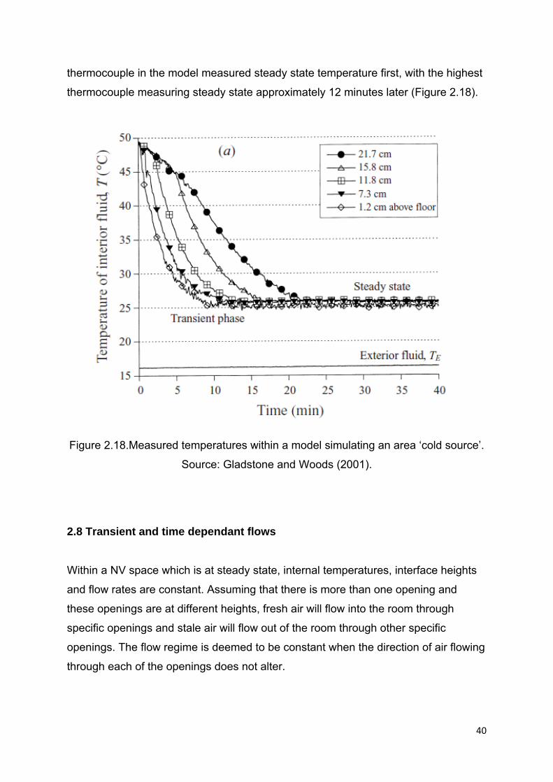
40
thermocouple in the model measured steady state temperature first, with the highest
thermocouple measuring steady state approximately 12 minutes later (Figure 2.18).
Figure 2.18.Measured temperatures within a model simulating an area ‘cold source’.
Source: Gladstone and Woods (2001).
2.8 Transient and time dependant flows
Within a NV space which is at steady state, internal temperatures, interface heights
and flow rates are constant. Assuming that there is more than one opening and
these openings are at different heights, fresh air will flow into the room through
specific openings and stale air will flow out of the room through other specific
openings. The flow regime is deemed to be constant when the direction of air flowing
through each of the openings does not alter.

41
If a change occurs within a space such as heat source strength or opening area,
then internal temperatures and flow rates through the space will change over time
until steady state is reached once more. In certain cases, the flow regime may switch
to a different one before reverting back. In such cases, the nature of the adjustment
in air flow and internal temperature is deemed to be transient. Whilst temporary,
transient flows may cause the internal thermal environment to become
uncomfortable for occupants until steady state is again reached. A better
understanding of transient flows may allow NV strategies to limit or prevent
occupants becoming uncomfortable during transient flows.
Specific circumstances such as a gust of wind or a change in location of heat source
may cause a flow regime at steady state to change permanently to a different one.
The new steady state will have different internal temperatures, flow rates and/or
interface heights from the original flow regime and could result in occupants having
an improved or worsened thermal comfort.
If a NV strategy is designed for a building with the intention to achieve a specific flow
regime ensuring a thermally comfortable and healthy environment for occupants, but
a different flow regime occurs, it can be very difficult to remedy. As a result, it is
important to better understand time dependent flows as this may inform as to
whether a NV design is susceptible to them. If multiple flow regimes at steady state
can exist in a natural ventilation strategy, then it is deemed to have multiple solutions,
which can be difficult to design for (Heiselberg et al. 2004).
2.8.1 Time dependant and transient air flows caused by the effect of wind.
This section describes how time dependant and transient air flows can be caused by
wind. Analytical methods (Yuan and Glicksman 2008, Heiselberg et al. 2004, Li et al.
2001, Li and Delsante 2001, Etheridge and Sandberg 1984), wind tunnel testing
(Chui and Etheridge 2004), CFD (Evola and Popov 2006, Jiang and Chen 2003,
Allocca et al 2003) and water bath modelling (Heiselberg et al 2003, Hunt and
Linden 1999) have been used to model the effects of wind on the air flow within a
building. In all models, there was significant agreement.
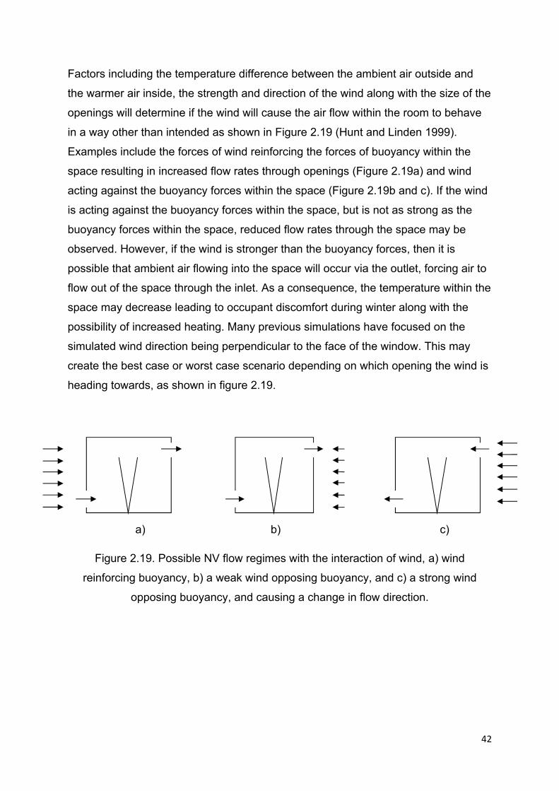
42
Factors including the temperature difference between the ambient air outside and
the warmer air inside, the strength and direction of the wind along with the size of the
openings will determine if the wind will cause the air flow within the room to behave
in a way other than intended as shown in Figure 2.19 (Hunt and Linden 1999).
Examples include the forces of wind reinforcing the forces of buoyancy within the
space resulting in increased flow rates through openings (Figure 2.19a) and wind
acting against the buoyancy forces within the space (Figure 2.19b and c). If the wind
is acting against the buoyancy forces within the space, but is not as strong as the
buoyancy forces within the space, reduced flow rates through the space may be
observed. However, if the wind is stronger than the buoyancy forces, then it is
possible that ambient air flowing into the space will occur via the outlet, forcing air to
flow out of the space through the inlet. As a consequence, the temperature within the
space may decrease leading to occupant discomfort during winter along with the
possibility of increased heating. Many previous simulations have focused on the
simulated wind direction being perpendicular to the face of the window. This may
create the best case or worst case scenario depending on which opening the wind is
heading towards, as shown in figure 2.19.
a) b) c)
Figure 2.19. Possible NV flow regimes with the interaction of wind, a) wind
reinforcing buoyancy, b) a weak wind opposing buoyancy, and c) a strong wind
opposing buoyancy, and causing a change in flow direction.

43
Figure 2.20.Effect of strong opposing wind from WBM using salt. (Source Hunt and
Linden 1999).
Figure 2.20 shows the effect of wind acting against the buoyancy forces within the
room, when the interior is at a fully mixed steady state. An interface forms as the
wind pushes the warmer than ambient internal air through the bottom opening, which
was originally acting as an inlet. For as long as the wind continues to blow in the
same direction, at a strength greater than the buoyancy forces of the warmer than
ambient air, the interface will continue to fall, until reaching the bottom of the room. If
the interface height lowers to a point where it interacts with the occupants, then it is
likely that the occupants will begin to feel thermally uncomfortable due to droughts.
Hunt and Linden (2004) modelled a simple room using water bath modelling with
brine to see if the effect of wind was different depending on if an interface had
already formed or not. Using a simple model and a single ‘point’ source, they allowed
an interface to form before directing wind towards the outlet. For low wind speed, the
flow rate through the space was simply reduced. Interestingly, they showed that with
an identical room, if the same heat source is used after the same wind source has
already started penetrating the outlet into the space, then instead of displacement
ventilation forming, the space became fully mixed. This is an important design
consideration for natural ventilation, showing that the effect of wind is considerably
stronger before an interface has formed. The laboratory configuration which
simulated wind within the salt bath experiment can be seen in Figure 2.21.
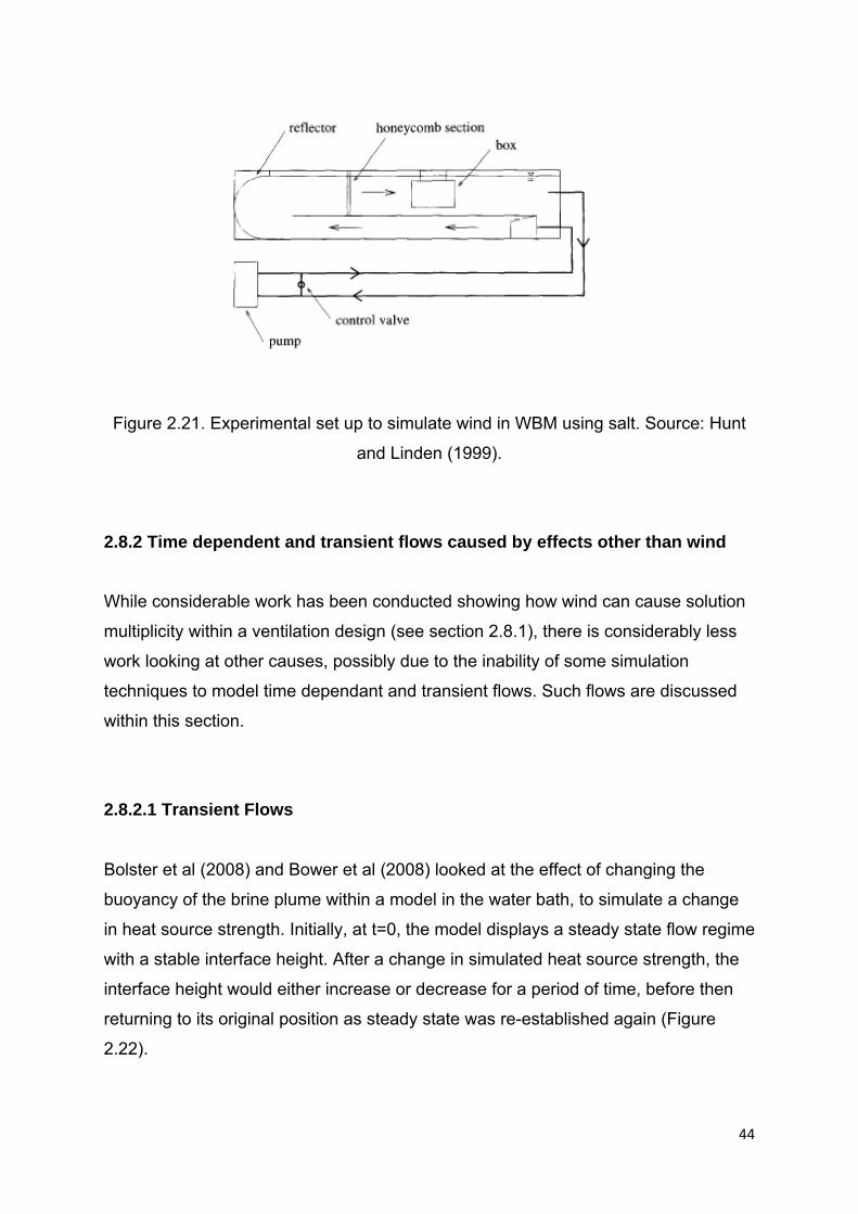
44
Figure 2.21. Experimental set up to simulate wind in WBM using salt. Source: Hunt
and Linden (1999).
2.8.2 Time dependent and transient flows caused by effects other than wind
While considerable work has been conducted showing how wind can cause solution
multiplicity within a ventilation design (see section 2.8.1), there is considerably less
work looking at other causes, possibly due to the inability of some simulation
techniques to model time dependant and transient flows. Such flows are discussed
within this section.
2.8.2.1 Transient Flows
Bolster et al (2008) and Bower et al (2008) looked at the effect of changing the
buoyancy of the brine plume within a model in the water bath, to simulate a change
in heat source strength. Initially, at t=0, the model displays a steady state flow regime
with a stable interface height. After a change in simulated heat source strength, the
interface height would either increase or decrease for a period of time, before then
returning to its original position as steady state was re-established again (Figure
2.22).
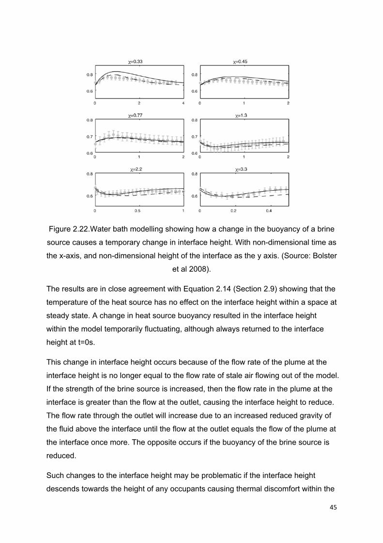
45
Figure 2.22.Water bath modelling showing how a change in the buoyancy of a brine
source causes a temporary change in interface height. With non-dimensional time as
the x-axis, and non-dimensional height of the interface as the y axis. (Source: Bolster
et al 2008).
The results are in close agreement with Equation 2.14 (Section 2.9) showing that the
temperature of the heat source has no effect on the interface height within a space at
steady state. A change in heat source buoyancy resulted in the interface height
within the model temporarily fluctuating, although always returned to the interface
height at t=0s.
This change in interface height occurs because of the flow rate of the plume at the
interface height is no longer equal to the flow rate of stale air flowing out of the model.
If the strength of the brine source is increased, then the flow rate in the plume at the
interface is greater than the flow at the outlet, causing the interface height to reduce.
The flow rate through the outlet will increase due to an increased reduced gravity of
the fluid above the interface until the flow at the outlet equals the flow of the plume at
the interface once more. The opposite occurs if the buoyancy of the brine source is
reduced.
Such changes to the interface height may be problematic if the interface height
descends towards the height of any occupants causing thermal discomfort within the
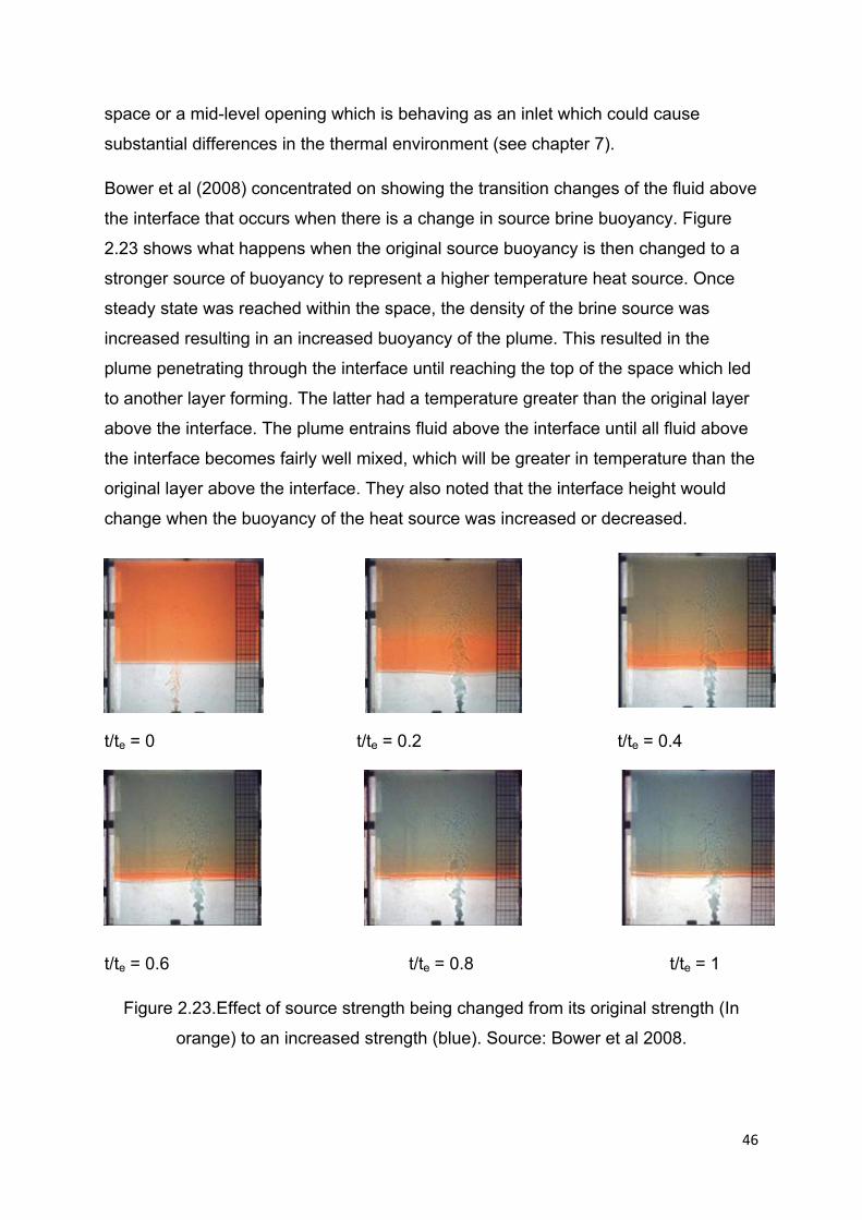
46
space or a mid-level opening which is behaving as an inlet which could cause
substantial differences in the thermal environment (see chapter 7).
Bower et al (2008) concentrated on showing the transition changes of the fluid above
the interface that occurs when there is a change in source brine buoyancy. Figure
2.23 shows what happens when the original source buoyancy is then changed to a
stronger source of buoyancy to represent a higher temperature heat source. Once
steady state was reached within the space, the density of the brine source was
increased resulting in an increased buoyancy of the plume. This resulted in the
plume penetrating through the interface until reaching the top of the space which led
to another layer forming. The latter had a temperature greater than the original layer
above the interface. The plume entrains fluid above the interface until all fluid above
the interface becomes fairly well mixed, which will be greater in temperature than the
original layer above the interface. They also noted that the interface height would
change when the buoyancy of the heat source was increased or decreased.
t/te = 0 t/te = 0.2 t/te = 0.4
t/te = 0.6 t/te = 0.8 t/te = 1
Figure 2.23.Effect of source strength being changed from its original strength (In
orange) to an increased strength (blue). Source: Bower et al 2008.
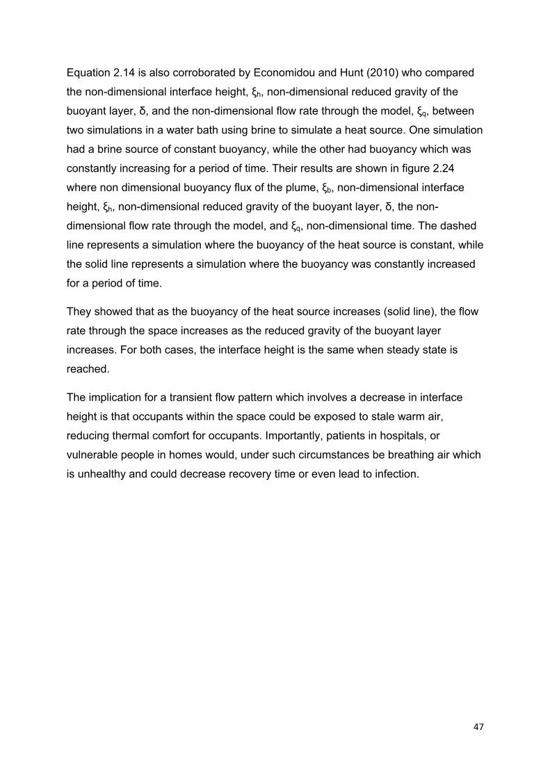
47
Equation 2.14 is also corroborated by Economidou and Hunt (2010) who compared
the non-dimensional interface height, ξh, non-dimensional reduced gravity of the
buoyant layer, δ, and the non-dimensional flow rate through the model, ξq, between
two simulations in a water bath using brine to simulate a heat source. One simulation
had a brine source of constant buoyancy, while the other had buoyancy which was
constantly increasing for a period of time. Their results are shown in figure 2.24
where non dimensional buoyancy flux of the plume, ξb, non-dimensional interface
height, ξh, non-dimensional reduced gravity of the buoyant layer, δ, the non-
dimensional flow rate through the model, and ξq, non-dimensional time. The dashed
line represents a simulation where the buoyancy of the heat source is constant, while
the solid line represents a simulation where the buoyancy was constantly increased
for a period of time.
They showed that as the buoyancy of the heat source increases (solid line), the flow
rate through the space increases as the reduced gravity of the buoyant layer
increases. For both cases, the interface height is the same when steady state is
reached.
The implication for a transient flow pattern which involves a decrease in interface
height is that occupants within the space could be exposed to stale warm air,
reducing thermal comfort for occupants. Importantly, patients in hospitals, or
vulnerable people in homes would, under such circumstances be breathing air which
is unhealthy and could decrease recovery time or even lead to infection.
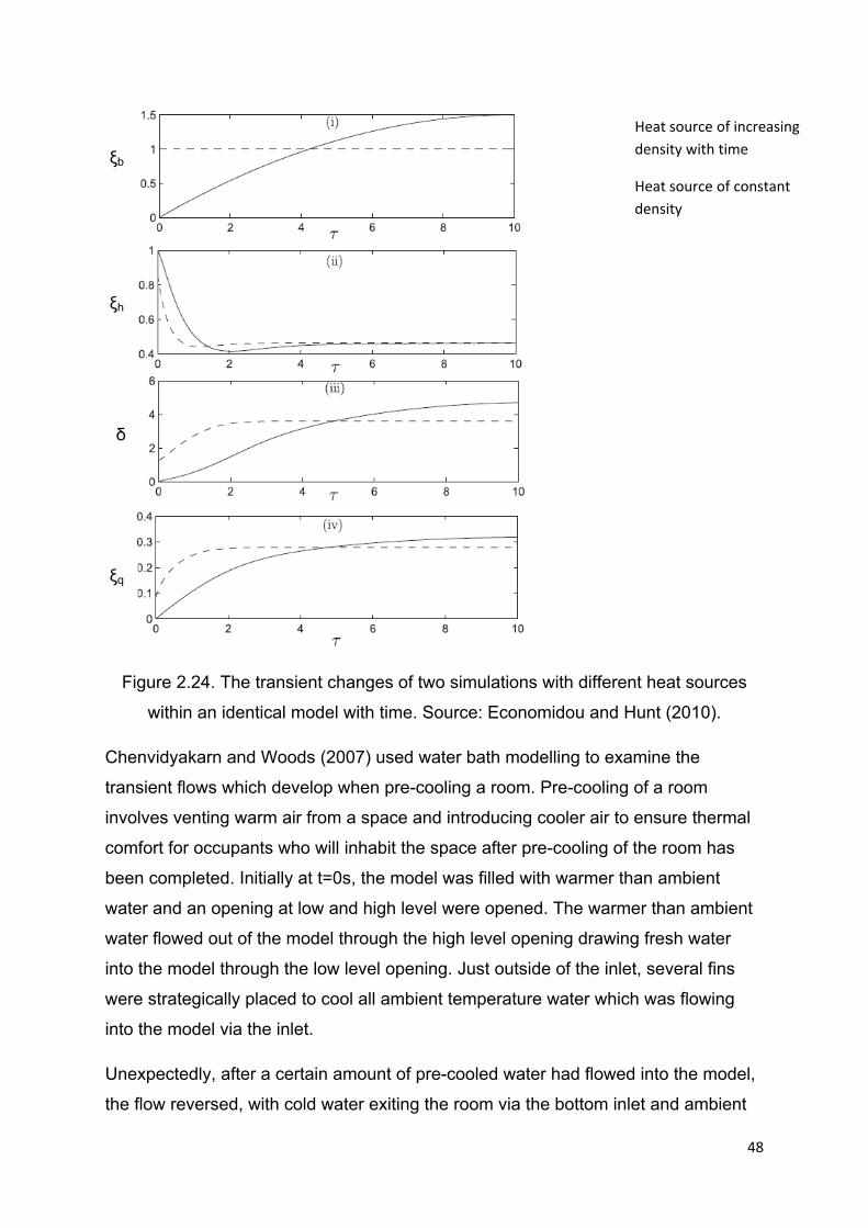
48
Figure 2.24. The transient changes of two simulations with different heat sources
within an identical model with time. Source: Economidou and Hunt (2010).
Chenvidyakarn and Woods (2007) used water bath modelling to examine the
transient flows which develop when pre-cooling a room. Pre-cooling of a room
involves venting warm air from a space and introducing cooler air to ensure thermal
comfort for occupants who will inhabit the space after pre-cooling of the room has
been completed. Initially at t=0s, the model was filled with warmer than ambient
water and an opening at low and high level were opened. The warmer than ambient
water flowed out of the model through the high level opening drawing fresh water
into the model through the low level opening. Just outside of the inlet, several fins
were strategically placed to cool all ambient temperature water which was flowing
into the model via the inlet.
Unexpectedly, after a certain amount of pre-cooled water had flowed into the model,
the flow reversed, with cold water exiting the room via the bottom inlet and ambient
Heat source of increasing
density with time
Heat source of constant
density
ξb
ξh
ξq
δ
49
outside water being drawn into the room through the outlet. After a certain point, the
flow reversed again and such flow reversals continued to occur until all the warmer
than ambient air had left the room. This switching between flow regimes resulted in
the space taking considerably longer to cool, and also resulted in increased energy
usage due to pre cooling of water which would flow out of the model through the low
level opening. Figure 2.25 shows this process in detail, with the red dyed
waterrepresenting warmer than ambient air within the model and black dyed fresh
water representing ambient exterior air which was sucked into the room via the outlet.
Figure 2.25.Water bath modelling showing the development of transitional flows
during pre-cooling of a room. (Source Chenvidyakarn, Woods 2007).
Fitzgerald and Woods (2010) considered a pre-heated room and conducted water
bath simulations with brine to analyse the transient flows which develop when a point
heat source is put into the room and openings at high and low level are opened.
They showed that one of four ‘modes’ can occur when a low and high opening are
opened simultaneously with a single point heat source being put into the room,
depending on the opening area, and the reduced gravity of the original fluid. This is
shown below in Figure 2.26.

50
Figure 2.26.Formation of four different flow regimes in a pre-heated room. Source:
Fitzegerald and Woods (2010).
The model was initially filled with brine to simulate the room being pre-heated and
brine of a greater density (representing a temperature higher than that of the pre-
heated room) flowed in to simulate a heat source within the space. In modes A and B,
the brine plume from the point brine source initially penetrates the brine layer within
the room and reaches the ceiling, but instead of a layer of denser brine forming at
the top of the model, all the brine from the brine source initially vents through the
outlet. At the same time fresh water starts flowing into the model through an inlet and
an interface forms and rises towards the ceiling.
After some time, a layer of denser brine begins to form just below the ceiling in Mode
A causing the formation of two interfaces within the model. The brine plume initially
entrains fresh water, then penetrates the lower interface and entrains the brine within
this layer before penetrating the upper interface. Eventually all the brine representing
the pre-heated air is entrained by the brine plume resulting in a single interface.
In Mode B, the density of the brine initially within the model is greater than in Mode A.
As a result, the brine plume entrains fresh water and becomes less dense than the
brine which was initially within the space. Two interfaces are observed again,
however the brine plume does not penetrate into the initial brine layer which vents
through the outlet. Instead, an ‘intrusion’ layer of brine forms below the original layer
of brine and builds up. Eventually, the initial brine layer fully vents out of the space
resulting in a single interface.

51
In modes C and D, the brine plume also penetrates the initial brine layer, but a layer
of dense brine forms immediately just below the ceiling. Except for this difference,
A&C, and B&D have similar transient flows.
Figure 2.27 shows when each of the modes will form depending on the non-
dimensional opening area ξa (Equation 2.32) and the non-dimensional reduced
gravity of the initial brine layer,δinitial(Equation 2.33). It should also be noted that the
different modes reached steady state at different times. Mode B was first to reach
steady state, followed by Mode D. Mode A and C reached steady state considerably
later.
Figure 2.27.The four different transitional flows which can form depending on the
non-dimensional opening area (ξa) and the reduced gravity of the original fluid within
the space g1. Source: Fitzegerald and Woods (2010).
ξa∗
2.32
δ g′ 2.33
δinitial
ξa
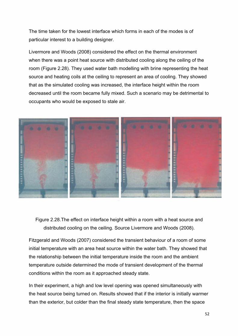
52
The time taken for the lowest interface which forms in each of the modes is of
particular interest to a building designer.
Livermore and Woods (2008) considered the effect on the thermal environment
when there was a point heat source with distributed cooling along the ceiling of the
room (Figure 2.28). They used water bath modelling with brine representing the heat
source and heating coils at the ceiling to represent an area of cooling. They showed
that as the simulated cooling was increased, the interface height within the room
decreased until the room became fully mixed. Such a scenario may be detrimental to
occupants who would be exposed to stale air.
Figure 2.28.The effect on interface height within a room with a heat source and
distributed cooling on the ceiling. Source Livermore and Woods (2008).
Fitzgerald and Woods (2007) considered the transient behaviour of a room of some
initial temperature with an area heat source within the water bath. They showed that
the relationship between the initial temperature inside the room and the ambient
temperature outside determined the mode of transient development of the thermal
conditions within the room as it approached steady state.
In their experiment, a high and low level opening was opened simultaneously with
the heat source being turned on. Results showed that if the interior is initially warmer
than the exterior, but colder than the final steady state temperature, then the space
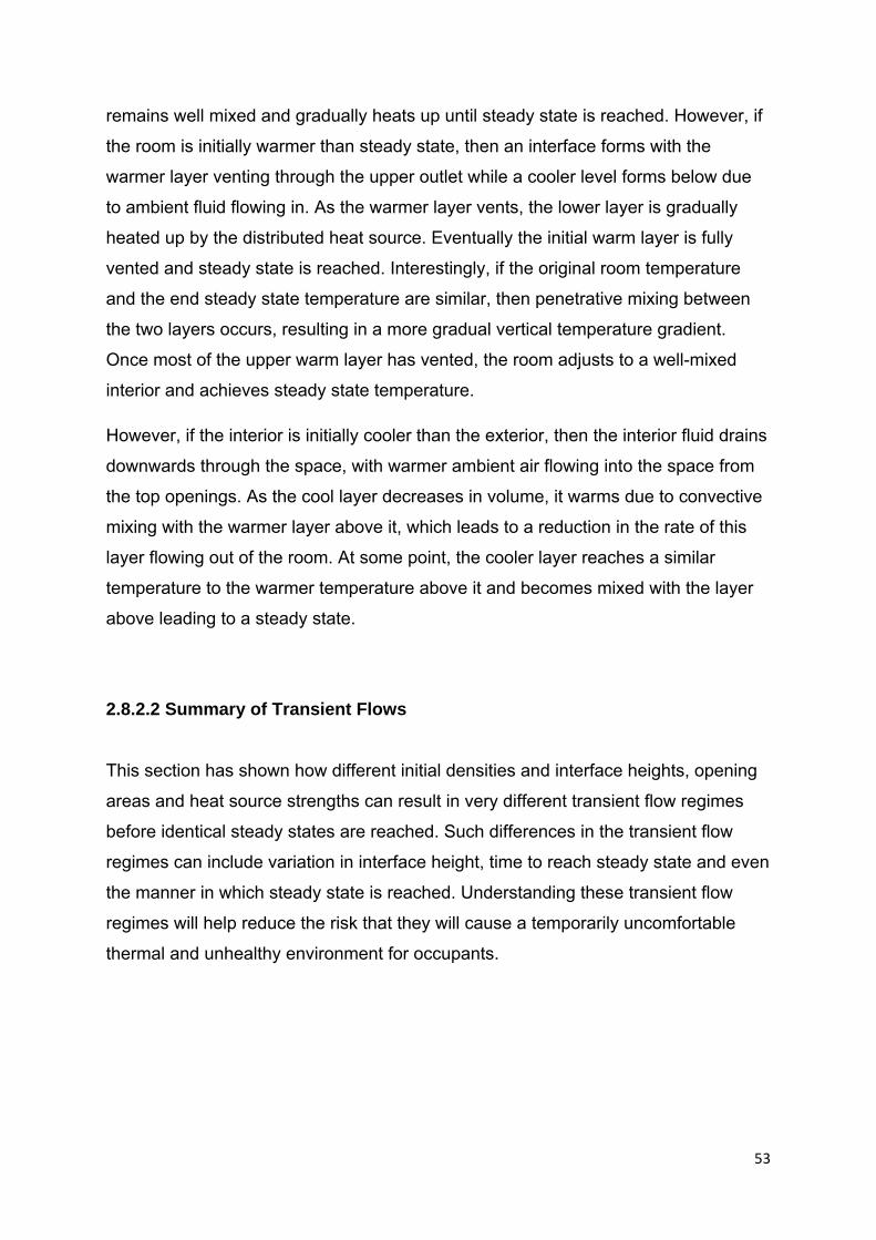
53
remains well mixed and gradually heats up until steady state is reached. However, if
the room is initially warmer than steady state, then an interface forms with the
warmer layer venting through the upper outlet while a cooler level forms below due
to ambient fluid flowing in. As the warmer layer vents, the lower layer is gradually
heated up by the distributed heat source. Eventually the initial warm layer is fully
vented and steady state is reached. Interestingly, if the original room temperature
and the end steady state temperature are similar, then penetrative mixing between
the two layers occurs, resulting in a more gradual vertical temperature gradient.
Once most of the upper warm layer has vented, the room adjusts to a well-mixed
interior and achieves steady state temperature.
However, if the interior is initially cooler than the exterior, then the interior fluid drains
downwards through the space, with warmer ambient air flowing into the space from
the top openings. As the cool layer decreases in volume, it warms due to convective
mixing with the warmer layer above it, which leads to a reduction in the rate of this
layer flowing out of the room. At some point, the cooler layer reaches a similar
temperature to the warmer temperature above it and becomes mixed with the layer
above leading to a steady state.
2.8.2.2 Summary of Transient Flows
This section has shown how different initial densities and interface heights, opening
areas and heat source strengths can result in very different transient flow regimes
before identical steady states are reached. Such differences in the transient flow
regimes can include variation in interface height, time to reach steady state and even
the manner in which steady state is reached. Understanding these transient flow
regimes will help reduce the risk that they will cause a temporarily uncomfortable
thermal and unhealthy environment for occupants.

54
2.8.2.3 Time dependant flows
If a ventilation strategy has achieved steady state, and a permanent or temporary
change occurs within the space, then the internal thermal conditions will change until
steady state is regained. If after steady state is reached again the flow regime is
different to the initial flow regime then the space is considered to have experienced a
time dependant flow.
Such changes could involve a change in strength or direction of wind entering the
space. These could cause a flow regime at steady state which has fresh air flowing
in at low level and stale air flowing out through a high level opening to reverse. This
means that fresh air begins to enter the room through a high level opening, and stale
air to flow out through the low level opening, which could, again, reduce thermal
comfort within the space as well as potentially increasing energy usage. As a result,
time dependent flows can cause a ventilation strategy to fail; ie: to act in a way that it
was not intended. Understanding these time dependent flows is important so that
future NV building designs can prevent them from occurring, or can be designed in
such a way to take advantage of these flows.
Chenvidyakarn and Woods (2005) used water bath simulations with an area heat
source to show how up to three different flow regimes can occur within a space due
to the effect of wind. Their model had two stacks of different heights, and a small low
level opening (Figure 2.29). Flow regime A involved fresh air flowing into the model
through the low level opening and short stack with stale air flowing out of the large
stack. Flow regime B had stale air flowing out of both stacks while in Regime C, stale
air only flowed out of the short stack.
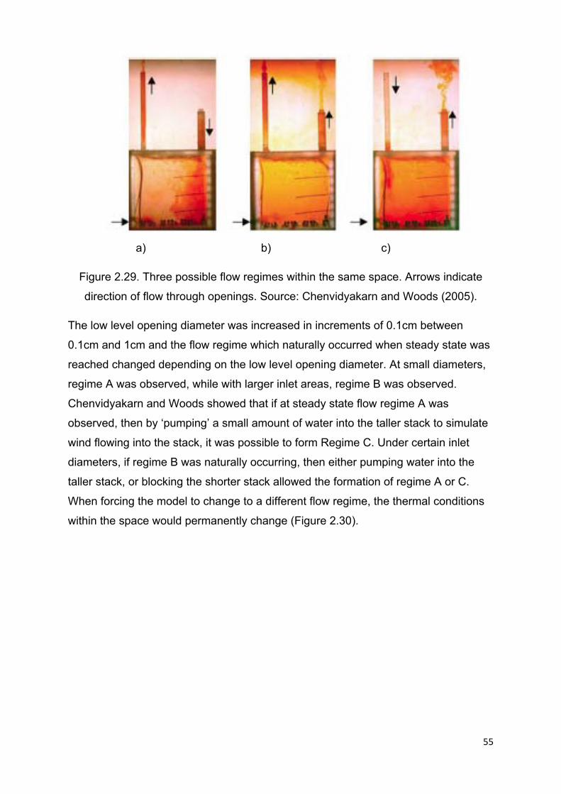
55
a) b) c)
Figure 2.29. Three possible flow regimes within the same space. Arrows indicate
direction of flow through openings. Source: Chenvidyakarn and Woods (2005).
The low level opening diameter was increased in increments of 0.1cm between
0.1cm and 1cm and the flow regime which naturally occurred when steady state was
reached changed depending on the low level opening diameter. At small diameters,
regime A was observed, while with larger inlet areas, regime B was observed.
Chenvidyakarn and Woods showed that if at steady state flow regime A was
observed, then by ‘pumping’ a small amount of water into the taller stack to simulate
wind flowing into the stack, it was possible to form Regime C. Under certain inlet
diameters, if regime B was naturally occurring, then either pumping water into the
taller stack, or blocking the shorter stack allowed the formation of regime A or C.
When forcing the model to change to a different flow regime, the thermal conditions
within the space would permanently change (Figure 2.30).

56
Figure 2.30.Theoretical and experimental dimensionless room temperatures for each
of the three regimes depending on the area of the bottom opening. Source:
Chenvidyakarn and Woods (2005).
Of note, it is tempting as a building designer to ensure that a shift in flow regimes is
prevented. However, on closer thought, being able to take advantage of such flow
regimes potentially enables improved thermal comfort within the space depending on
heat load and ambient temperatures.
Chenvidyakarn and Woods (2010) further considered two rooms connected by an
opening at low level, with both rooms having an opening at high level at the same
height. They used water bath modelling with an area heat source to simulate
different flow regimes within the space. They showed that if both rooms had an
identical heat source within it, then flow through the space could happen in either
direction (Figure 2.31). It was then possible to reverse the flow regime by simulating
wind entering the outlet of the room downstream of the flow.
Dim
ensi
onle
ss r
oom
tem
pera
ture
Area of bottom opening A*3/A
*1
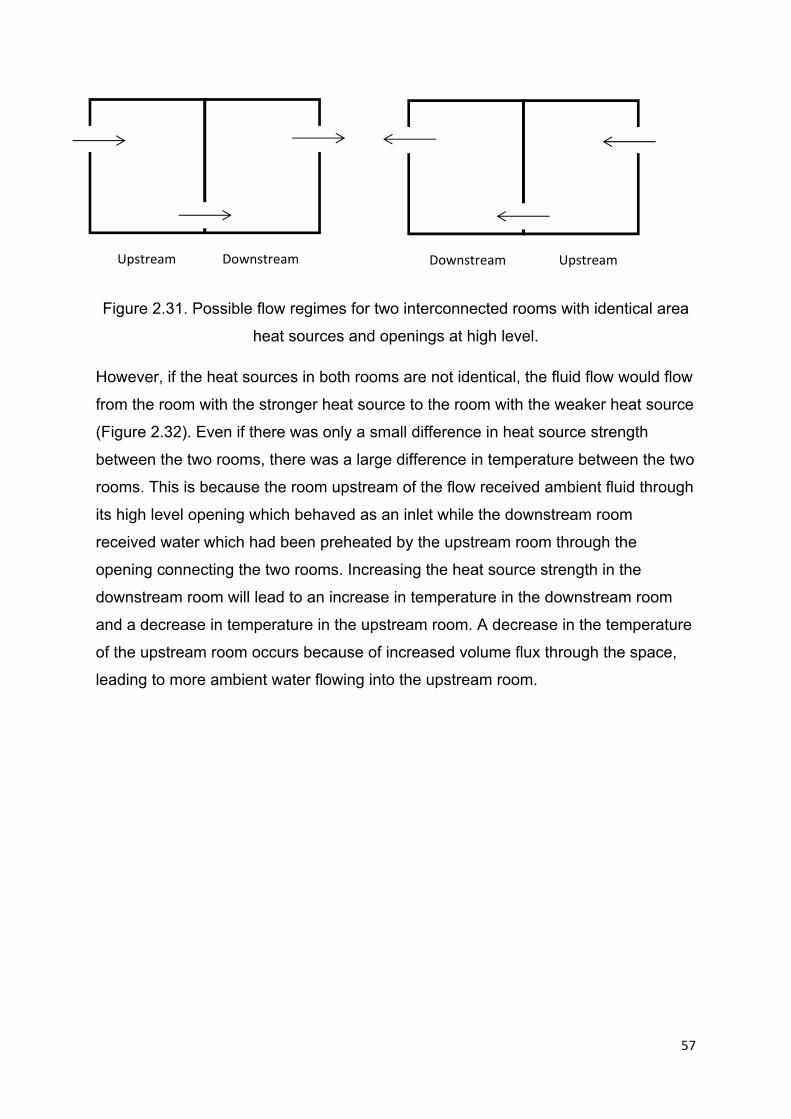
57
Figure
Figure 2.31. Possible flow regimes for two interconnected rooms with identical area
heat sources and openings at high level.
However, if the heat sources in both rooms are not identical, the fluid flow would flow
from the room with the stronger heat source to the room with the weaker heat source
(Figure 2.32). Even if there was only a small difference in heat source strength
between the two rooms, there was a large difference in temperature between the two
rooms. This is because the room upstream of the flow received ambient fluid through
its high level opening which behaved as an inlet while the downstream room
received water which had been preheated by the upstream room through the
opening connecting the two rooms. Increasing the heat source strength in the
downstream room will lead to an increase in temperature in the downstream room
and a decrease in temperature in the upstream room. A decrease in the temperature
of the upstream room occurs because of increased volume flux through the space,
leading to more ambient water flowing into the upstream room.
Upstream Downstream Downstream Upstream

58
Figure 2.32. Flow regime and development of internal temperatures within
geometrically identical interconnected rooms with different area heat sources.
Source: Chenvidyakarn and Woods (2010).
Interestingly, the history of the flow also determines whether or not a change in flow
regime occurs. Initially room B had a larger heat source than room A to ensure that
room B was downstream of the flow. After steady state was reached, the heat source
strength in room A was then increased beyond the heat source strength in room B
but the flow regime did not change and room A remained lower in temperature than
in room B. Only when the heat source in room A was 100W greater than in room B,
did the temperature in room A increase beyond that of room B and did the flow
regime switch so that room A became downstream of the flow (Figure 2.33).

59
Figure 2.33.Temperature within room A and B depending on the history of flow with
varying heat source strength in room A. Source: Chenvidyakarn and Woods (2010).
Increasing the heat source strength in the upstream room will lead to a temperature
increase in both rooms, however such increases may lead to a switch in flow regime
which can then lead to a significant cooling effect in the room which was originally
downstream (Figure 2.34). As the flow regime switches, there is a transitional period,
where the upper openings in both rooms experience bi-directional flow. During this
time, there is a significant change in temperature in both rooms resulting in flow
regime changing.
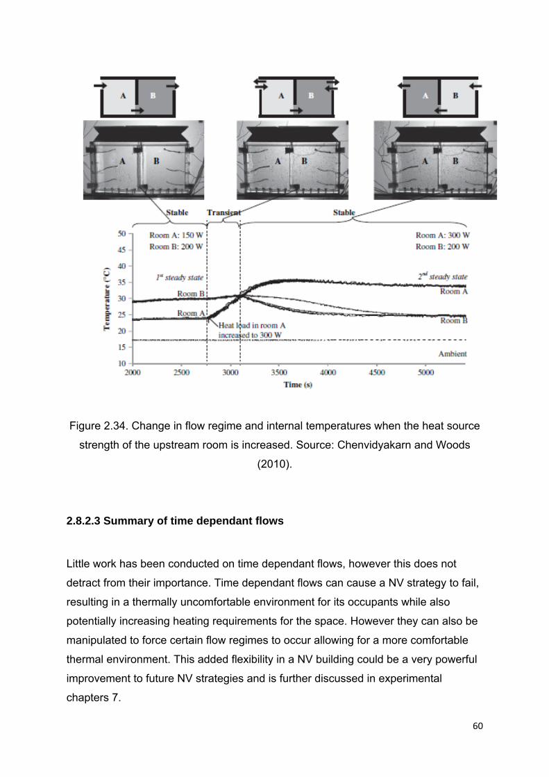
60
Figure 2.34. Change in flow regime and internal temperatures when the heat source
strength of the upstream room is increased. Source: Chenvidyakarn and Woods
(2010).
2.8.2.3 Summary of time dependant flows
Little work has been conducted on time dependant flows, however this does not
detract from their importance. Time dependant flows can cause a NV strategy to fail,
resulting in a thermally uncomfortable environment for its occupants while also
potentially increasing heating requirements for the space. However they can also be
manipulated to force certain flow regimes to occur allowing for a more comfortable
thermal environment. This added flexibility in a NV building could be a very powerful
improvement to future NV strategies and is further discussed in experimental
chapters 7.

61
2.9 Conclusion of Chapter
This chapter has briefly looked at the history of how humans have always tried to
control their living environment to make it as comfortable as possible. For the latter
part of the 20th Century, air conditioning became the predominant technology used
to control ventilation, especially in hot and humid climates such as Singapore.
However, as our awareness of global warming developed in the latter part of the
century and early 21st century, it is apparent that natural ventilation offers a better
future.
The principles of natural ventilation were explored with particular attention to the
research of Linden, Woods, Chenvidyakarn, Kaye, Fitzgerald and Hunt. Transient
and time dependant flow regimes were discussed with a focus on how they can
cause internal temperatures, air flow rates and interface heights within a naturally
ventilated building to be different than what was intended during the design of the
ventilation strategy. While transient flow regimes are temporary they can still cause
occupants to be exposed to thermal uncomfortable and stale air for a short period of
time and are important to limit. Time dependant flow regimes can be catastrophic for
a naturally ventilated building leading to steady state flows being completely different
to what was intended.
The experimental results from simulations conducted within this research will be
compared with the theory discussed within this section. This is important to provide
confidence that the Water Bath Modelling Facility is accurately simulating a NV
space.
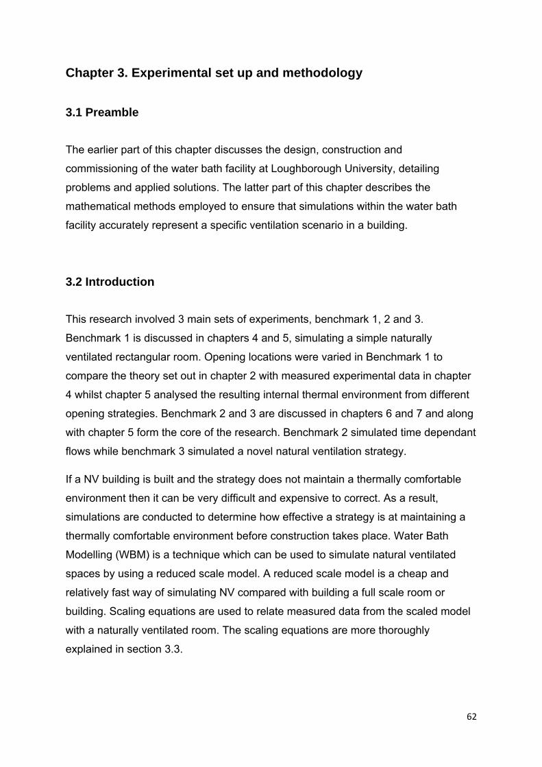
62
Chapter 3. Experimental set up and methodology
3.1 Preamble
The earlier part of this chapter discusses the design, construction and
commissioning of the water bath facility at Loughborough University, detailing
problems and applied solutions. The latter part of this chapter describes the
mathematical methods employed to ensure that simulations within the water bath
facility accurately represent a specific ventilation scenario in a building.
3.2 Introduction
This research involved 3 main sets of experiments, benchmark 1, 2 and 3.
Benchmark 1 is discussed in chapters 4 and 5, simulating a simple naturally
ventilated rectangular room. Opening locations were varied in Benchmark 1 to
compare the theory set out in chapter 2 with measured experimental data in chapter
4 whilst chapter 5 analysed the resulting internal thermal environment from different
opening strategies. Benchmark 2 and 3 are discussed in chapters 6 and 7 and along
with chapter 5 form the core of the research. Benchmark 2 simulated time dependant
flows while benchmark 3 simulated a novel natural ventilation strategy.
If a NV building is built and the strategy does not maintain a thermally comfortable
environment then it can be very difficult and expensive to correct. As a result,
simulations are conducted to determine how effective a strategy is at maintaining a
thermally comfortable environment before construction takes place. Water Bath
Modelling (WBM) is a technique which can be used to simulate natural ventilated
spaces by using a reduced scale model. A reduced scale model is a cheap and
relatively fast way of simulating NV compared with building a full scale room or
building. Scaling equations are used to relate measured data from the scaled model
with a naturally ventilated room. The scaling equations are more thoroughly
explained in section 3.3.

63
Within a NV room, a heat source will heat the air around it causing density
differences which leads to the warmer than ambient air rising. Similar density
differences must also be created within the reduced scale model to simulate a heat
source. WBM can simulate a heat source by either injecting another fluid of a
different density to water within the model, or by installing heating/cooling wires
within the model to create density differences. Both methods can cause the
formation of a plume of fluid which is of a different density to fresh water within the
model. Brine (salt water) is usually chosen as the fluid to be injected into the model
because it is cheap to produce, and large density differences can be created (brine
can be 30% denser than fresh water). The importance of being able to achieve such
large density differences is further explained in section 3.3.
Figure 3.1 shows that as air or water is heated by a person or other heat source, the
fluid rises because of a reduction in density. Brine is denser than fresh water and will
sink to the bottom of the model while hot air and hot water will float towards the top
of the model. As a result, models which use brine to simulate a heat source are
inverted, so that the floor of the model is at the top, and the roof of the model is at
the bottom. Assuming that the heat source is on the floor, the plume produced by a
heat source travels vertically upwards, but the plume produced by brine travels
vertically downwards. This means that the brine plume is negatively buoyant. This
reversal in buoyancy means that flows occur upside down.

64
a) b) c)
Figure 3.1. Plume formation for: a) a hot air plume caused by a human within a room,
b) a heated wire (Orange box) heating water around it and c) a brine source.
From this point onwards in this chapter, the NV room or building which is to be
simulated will be described as ‘full scale’, and the model within the water bath
described as ‘reduced scale’. Where in an equation, subscript ‘f’ refers to full scale
and subscript ‘m’ refers to reduced scale. In all simulations presented in this work, a
heat source was represented by injecting brine into the model. The brine was dyed
using food dye to improve visualisation. In all future schematic diagrams, brine is
represented in red, while fresh water is represented in blue.
3.3 Scaling equations
Brine within a reduced scale model is used to represent heated air at full scale.
Scaling equations relate the density of the brine at reduced scale, to the density of
air at full scale.
3.3.1 Exact simulation scaling
In order to ensure that the WBM simulation is accurately representing the full scale
scenario that we wish to simulate, the model’s dimensions must be scaled to the full
sized room dimensions. Next, kinematic similarity between the model and the full
Floor
Roof
Floor Roof
Roof Roof

65
sized scenario is required. To achieve kinematic similarity, it is suggested that
Prandtl numbers (Pr – ratio of viscous diffusion and thermal diffusion), Reynolds
numbers (Re – ratio of inertial forces and viscous forces), and Archimedes numbers
(Ar – ratio of buoyancy forces to viscous forces) should be made equal between the
model and full scales (Awbi 2003). However, because the fluid changes between full
scale and model scale (air to water), it is impossible to match Pr. It is possible to
match Re and Ar and this is noted in other research as being sufficient to ensure that
a full scale scenario is accurately represented within model scale (Walker 2005). To
calculate Reynolds numbers, Archimedes numbers and Prandtl, equation 3.1, 3.2
and 3.3 can be used, where subscripts ‘m’ and ‘f’ refer to model and full scale values:
, 3.1
, ∆ ∆ 3.2
, 3.3
Where is the kinematic viscosity (m2/s), μ is the dynamic viscosity (kg/m.s) and α is
the thermal diffusivity (m2/s). By calculating the Reynolds number and the
Archimedes number for the reduced scale simulation, the equations can be re-
arranged to calculate or ∆ .
To ensure that and , a four-step iterative procedure was
followed and is described below. Following this procedure will ensure that the flow
within the model is accurately represented by air flow at full scale.
Step 1: Calculate the Archimedes (Ar) and Reynolds (Re) numbers for the scaled
model
The effective opening area ( ∗ ) of the model needs be calculated and is found using
Equation 3.4 which is provided by Linden et al. (1990) as:

66
∗ .
3.4
where Cd1 and Cd2 is the discharge coefficient to account for vena contracta through
openings a1 at low level and a2 at high level. In order to achieve kinematic similarity,
initial values for density of the brine, ρ0 and flow rate, Fm must be chosen. These
values will likely be changed later on in this four step process. The buoyancy flux of
brine plume Bm, is calculated using Equation 3.5:
, 3.5
where subscript ‘o’ denotes initial values of brine before it enters the scaled model, ρ
is the density of the ambient fluid (kg/m3) and T is the temperature of the ambient
fluid (K). To calculate the approximate interface height to be observed within the
scaled model, hm, the ratio between effective opening area ( ∗ ) and the height
between the heat source (including the virtual origin) and upper opening ( ∗ ) was
utilised as shown in Equation 3.6(Linden et al. 1990).
∗ 3.6
The reduced gravity (g’) of the brine below the interface can then be calculated using
Equation 3.7.
3.7
Where C is a constant derived by Morton, et al. 1956 and can be taken to be 0.158.
The source Archimedes equation to account for the addition of brine into the space is
shown as Equation 3.8(Hunt et al. 2001):
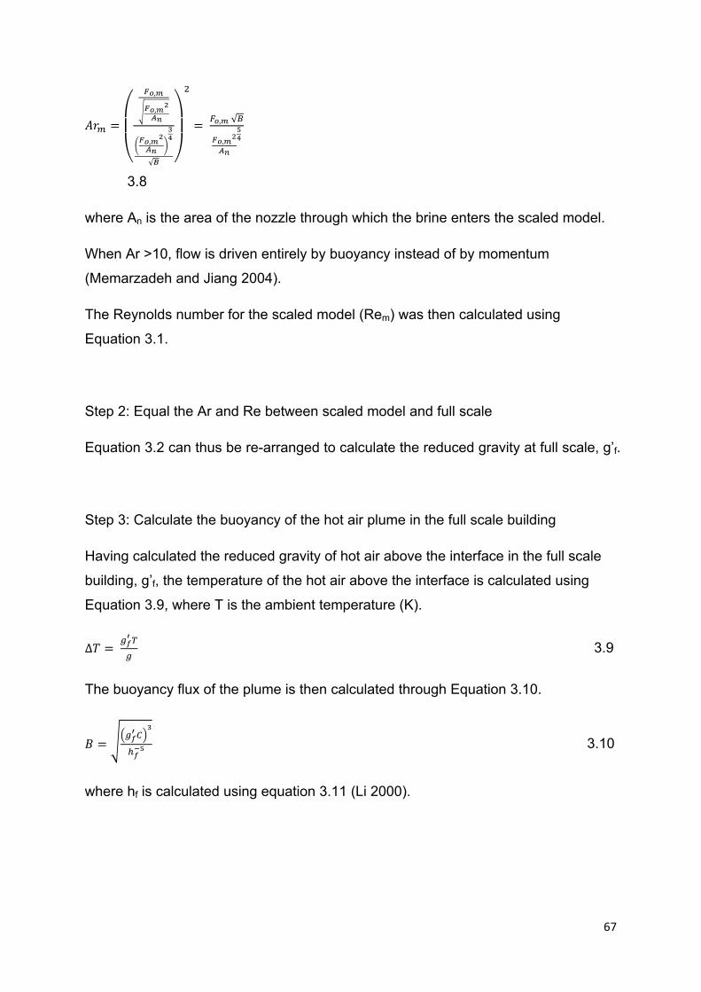
67
,
,
,
√
, √
,
3.8
where An is the area of the nozzle through which the brine enters the scaled model.
When Ar >10, flow is driven entirely by buoyancy instead of by momentum
(Memarzadeh and Jiang 2004).
The Reynolds number for the scaled model (Rem) was then calculated using
Equation 3.1.
Step 2: Equal the Ar and Re between scaled model and full scale
Equation 3.2 can thus be re-arranged to calculate the reduced gravity at full scale, g’f.
Step 3: Calculate the buoyancy of the hot air plume in the full scale building
Having calculated the reduced gravity of hot air above the interface in the full scale
building, g’f, the temperature of the hot air above the interface is calculated using
Equation 3.9, where T is the ambient temperature (K).
∆ 3.9
The buoyancy flux of the plume is then calculated through Equation 3.10.
3.10
where hf is calculated using equation 3.11 (Li 2000).
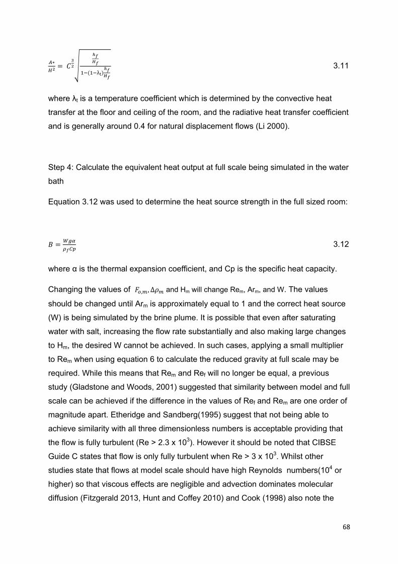
68
∗
λt 3.11
where λt is a temperature coefficient which is determined by the convective heat
transfer at the floor and ceiling of the room, and the radiative heat transfer coefficient
and is generally around 0.4 for natural displacement flows (Li 2000).
Step 4: Calculate the equivalent heat output at full scale being simulated in the water
bath
Equation 3.12 was used to determine the heat source strength in the full sized room:
3.12
where α is the thermal expansion coefficient, and Cp is the specific heat capacity.
Changing the values of , , ∆ and Hm will change Rem, Arm, and W. The values
should be changed until Arm is approximately equal to 1 and the correct heat source
(W) is being simulated by the brine plume. It is possible that even after saturating
water with salt, increasing the flow rate substantially and also making large changes
to Hm, the desired W cannot be achieved. In such cases, applying a small multiplier
to Rem when using equation 6 to calculate the reduced gravity at full scale may be
required. While this means that Rem and Ref will no longer be equal, a previous
study (Gladstone and Woods, 2001) suggested that similarity between model and full
scale can be achieved if the difference in the values of Ref and Rem are one order of
magnitude apart. Etheridge and Sandberg(1995) suggest that not being able to
achieve similarity with all three dimensionless numbers is acceptable providing that
the flow is fully turbulent (Re > 2.3 x 10³). However it should be noted that CIBSE
Guide C states that flow is only fully turbulent when Re > 3 x 10³. Whilst other
studies state that flows at model scale should have high Reynolds numbers(104 or
higher) so that viscous effects are negligible and advection dominates molecular
diffusion (Fitzgerald 2013, Hunt and Coffey 2010) and Cook (1998) also note the

69
importance of achieving dynamic similarity between model and full scale. This can
be achieved by using equations which form ratios, including equation 3.14.
3.14
where and are the velocity of the fluid within model and full scale (m/s).
The example below shows that similar Archimedes and Rayleigh numbers between
model and full scale can be achieved, whilst ensuring sufficiently turbulent flow.
If Hm is 0.3m, A* = 0.0001564m2, density of brine at the source is 1100 kg/m3 with
a flow rate of 2 cm3/s, the theoretical interface height (before virtual origin
correction) is 0.09m (equation 2.13).
The virtual origin is calculated as 0.015m (equation 2.22) when the nozzle has a
0.005m diameter.
Arm becomes 1.29 and Re is 2.64 x 10⁴, meaning that the flow within the scaled
model is predominantly driven by buoyancy forces and the flow is fully turbulent. If Hf
is 3m, with an ambient air temperature of 20 °C and a multiplier of 6.5 is applied to
Ref, (Ref = 1.9 x 10⁵) then hf = 0.74m, the temperature above the interface is 26°C
and the heat source at full scale is 50W.
If brine is observed to flow out of the model at 0.05m/s, then according to the ratio
scaling, the speed of hot air flowing out at full scale should be about 0.15m/s.
If a simulation has been run, with interface heights and density below the interface
measured at steady state, it is possible to rearrange the above four step process to
determine the simulated thermal environment at full scale including internal
temperatures and the strength of the heat source.

70
3.3.2 Non dimensional scaling
For simulations where the four step process can not be successfully calculated (for
example when similarity can not be achieved), dimensionless quantities are used to
compare data between simulations and theory. Fitzgerald and Woods (2007) and
Woods and Chenvidyakarn (2005) used non-dimensional temperatures, with the
latter using equation 3.15 to compare a 90W heat source within a small model with
theoretical equations for a full scale room with a very large heat source.
ξ,
3.15
∗, , 3.16
where Tin is the internal temperature, Te is the external temperature, Tin,ssis the
internal temperature at steady state and Th is the observed temperature at the heat
source. Equation 3.15 allows for comparisons with how the internal temperature
varies with time until steady state is reached, while equation 3.16 allows for
comparisons with the final steady state temperature.
3.4. Experimental set up
Figure 3.2 shows the experimental set up of the water bath facility. Brine is stored in
a reservoir tank which has a capacity of 30 litres. The tank is at low level to allow for
easy access for density measurements to ensure that the brine is of the intended
density calculated in section 3.3.1. The brine is then pumped to a header tank
suspended at 3.5m. The header tank contains an overflow pipe which feeds brine
back to the reservoir, ensuring a constant amount of brine within the header tank. An
analogue flow meter is used to control the volume flow rate of brine into the model
from the header tank. The model was suspended in a large acrylic tank.
The acrylic tank has dimensions 1 x 1.4 x 1.6m with a thickness of 0.03m. This
thickness caused very small parallax errors, which meant that objects within the tank
appeared to be in different positions when looking at the object from different angles.
The parallax errors were significantly increased when the tank was filled with water.

71
Such large errors can potentially cause inaccuracies when attempting to determine
the interface height within the model. Parallax errors affecting the accuracy of
interface readings were minimized by having eye level at a perpendicular position to
the interface height.
Figure 3.2. Experimental set up of water bath facility at Loughborough University.
Plinth
Water tank
Model
Header tank
Overflow pipe
1.4m
1.6m
1.1m
0.2m
Reservoir tank
Pump
Flow meter
0.5m

72
3.4.1 Large water reservoir
The reduced scale perspex model was suspended near the top of the acrylic tank.
During simulations, brine would build up inside the model, creating a layer of dense
fluid which would drive flow through the openings of the model. Brine flowing out of
the model flowed to the bottom of the acrylic tank and with time, a layer of brine built
up at the bottom of the tank as shown in figure 3.3. The tank was tall, allowing for as
many simulations to be conducted as possible until the build-up of brine at the
bottom of the tank had risen to a point where the spent brine was interacting with the
suspended model.
Figure 3.3.Build-up of brine (dyed red) in the large acrylic tank during a simulation.
As the brine fell towards the bottom of the tank, more than expected mixing between
the brine and fresh water took place. This meant that a layer of brine at the bottom of
the tank built up much more quickly than anticipated. This limited how many
simulations could be run before the tank would have to be emptied and refilled, a
process which takes approximately two hours. This was noted by other researchers
conducting water bath simulations (Kaye and Hunt 2009), and they overcame this by
using pipes to siphon off the brine at the bottom of the tank, replacing this brine with
fresh water, carefully inserted near the top of the tank to limit turbulence (Figure 3.4).
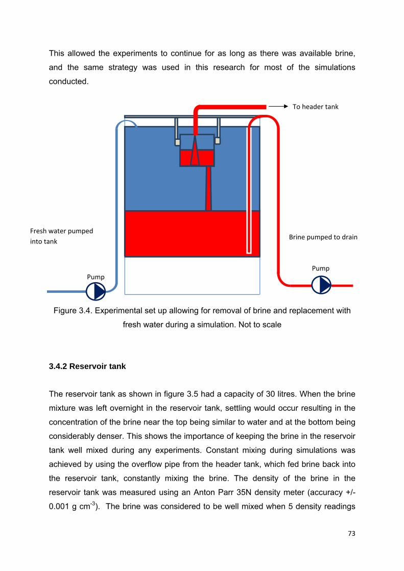
73
This allowed the experiments to continue for as long as there was available brine,
and the same strategy was used in this research for most of the simulations
conducted.
Figure 3.4. Experimental set up allowing for removal of brine and replacement with
fresh water during a simulation. Not to scale
3.4.2 Reservoir tank
The reservoir tank as shown in figure 3.5 had a capacity of 30 litres. When the brine
mixture was left overnight in the reservoir tank, settling would occur resulting in the
concentration of the brine near the top being similar to water and at the bottom being
considerably denser. This shows the importance of keeping the brine in the reservoir
tank well mixed during any experiments. Constant mixing during simulations was
achieved by using the overflow pipe from the header tank, which fed brine back into
the reservoir tank, constantly mixing the brine. The density of the brine in the
reservoir tank was measured using an Anton Parr 35N density meter (accuracy +/-
0.001 g cm-3). The brine was considered to be well mixed when 5 density readings
Brine pumped to drain Fresh water pumped
into tank
To header tank
Pump Pump

74
from the Anton Parr device varied by no more than ± 0.0003g/cm3; this was usually
achieved after 20 minutes of mixing caused by the overflow pipe. If the density of the
brine in the reservoir was not constant, then the buoyancy of the brine plume within
the model will vary as shown by equation 3.5. If the buoyancy at the brine source
varies throughout the simulation, then the equivalent heat source at full scale will
vary with time. This will cause fluctuations in the interface (described in section
2.7.2.1) along with variations in density above the interface.
‘
Figure 3.5.Reservoir tank for storage and continued mixing of brine during water
bath simulations.
The reservoir tank was ideal for simulations lasting up to an hour with no more than
4 nozzles, each representing a 50W heat source.
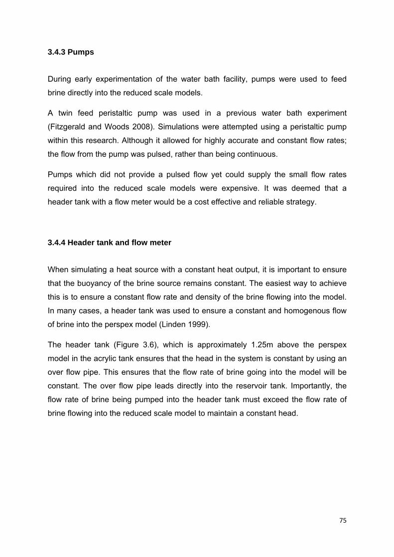
75
3.4.3 Pumps
During early experimentation of the water bath facility, pumps were used to feed
brine directly into the reduced scale models.
A twin feed peristaltic pump was used in a previous water bath experiment
(Fitzgerald and Woods 2008). Simulations were attempted using a peristaltic pump
within this research. Although it allowed for highly accurate and constant flow rates;
the flow from the pump was pulsed, rather than being continuous.
Pumps which did not provide a pulsed flow yet could supply the small flow rates
required into the reduced scale models were expensive. It was deemed that a
header tank with a flow meter would be a cost effective and reliable strategy.
3.4.4 Header tank and flow meter
When simulating a heat source with a constant heat output, it is important to ensure
that the buoyancy of the brine source remains constant. The easiest way to achieve
this is to ensure a constant flow rate and density of the brine flowing into the model.
In many cases, a header tank was used to ensure a constant and homogenous flow
of brine into the perspex model (Linden 1999).
The header tank (Figure 3.6), which is approximately 1.25m above the perspex
model in the acrylic tank ensures that the head in the system is constant by using an
over flow pipe. This ensures that the flow rate of brine going into the model will be
constant. The over flow pipe leads directly into the reservoir tank. Importantly, the
flow rate of brine being pumped into the header tank must exceed the flow rate of
brine flowing into the reduced scale model to maintain a constant head.
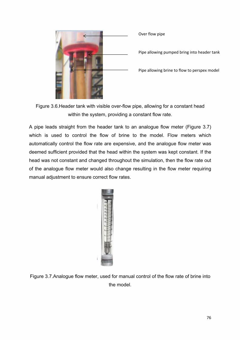
76
Figure 3.6.Header tank with visible over-flow pipe, allowing for a constant head
within the system, providing a constant flow rate.
A pipe leads straight from the header tank to an analogue flow meter (Figure 3.7)
which is used to control the flow of brine to the model. Flow meters which
automatically control the flow rate are expensive, and the analogue flow meter was
deemed sufficient provided that the head within the system was kept constant. If the
head was not constant and changed throughout the simulation, then the flow rate out
of the analogue flow meter would also change resulting in the flow meter requiring
manual adjustment to ensure correct flow rates.
Figure 3.7.Analogue flow meter, used for manual control of the flow rate of brine into
the model.
Over flow pipe
Pipe allowing pumped bring into header tank
Pipe allowing brine to flow to perspex model
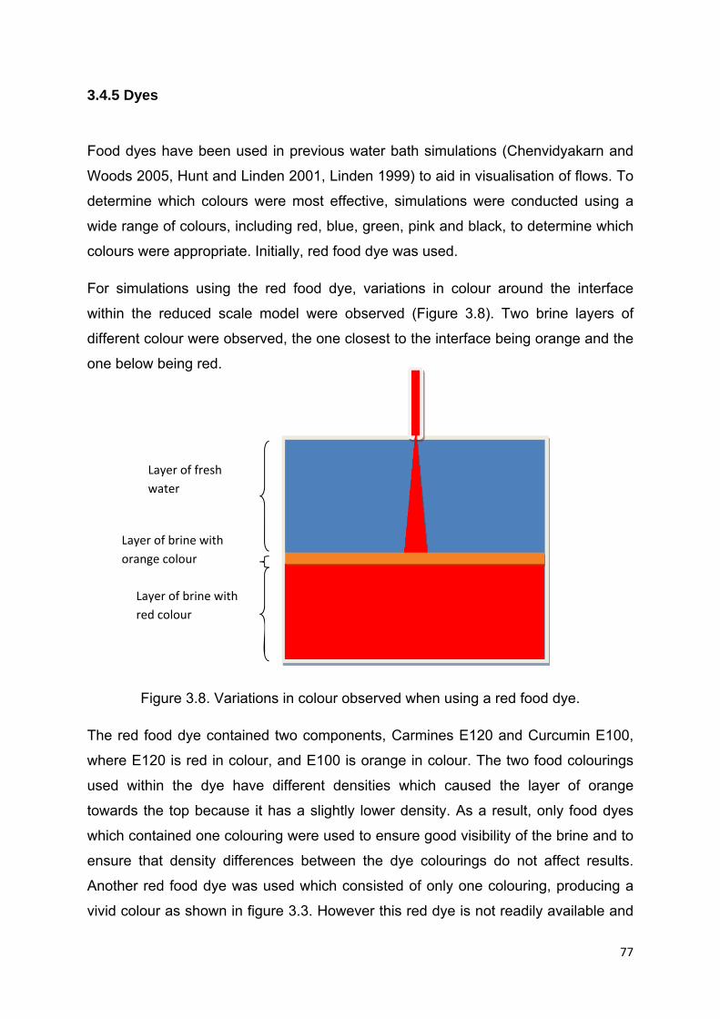
77
3.4.5 Dyes
Food dyes have been used in previous water bath simulations (Chenvidyakarn and
Woods 2005, Hunt and Linden 2001, Linden 1999) to aid in visualisation of flows. To
determine which colours were most effective, simulations were conducted using a
wide range of colours, including red, blue, green, pink and black, to determine which
colours were appropriate. Initially, red food dye was used.
For simulations using the red food dye, variations in colour around the interface
within the reduced scale model were observed (Figure 3.8). Two brine layers of
different colour were observed, the one closest to the interface being orange and the
one below being red.
Figure 3.8. Variations in colour observed when using a red food dye.
The red food dye contained two components, Carmines E120 and Curcumin E100,
where E120 is red in colour, and E100 is orange in colour. The two food colourings
used within the dye have different densities which caused the layer of orange
towards the top because it has a slightly lower density. As a result, only food dyes
which contained one colouring were used to ensure good visibility of the brine and to
ensure that density differences between the dye colourings do not affect results.
Another red food dye was used which consisted of only one colouring, producing a
vivid colour as shown in figure 3.3. However this red dye is not readily available and
Layer of fresh
water
Layer of brine with
orange colour
Layer of brine with
red colour
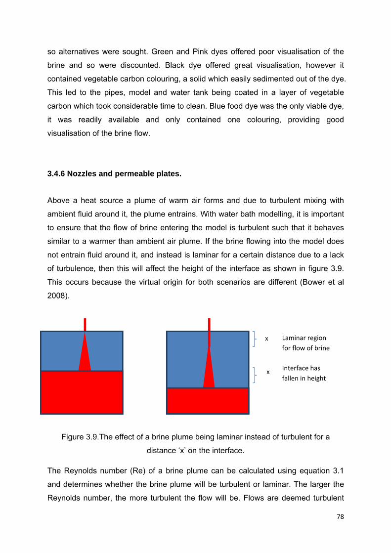
78
so alternatives were sought. Green and Pink dyes offered poor visualisation of the
brine and so were discounted. Black dye offered great visualisation, however it
contained vegetable carbon colouring, a solid which easily sedimented out of the dye.
This led to the pipes, model and water tank being coated in a layer of vegetable
carbon which took considerable time to clean. Blue food dye was the only viable dye,
it was readily available and only contained one colouring, providing good
visualisation of the brine flow.
3.4.6 Nozzles and permeable plates.
Above a heat source a plume of warm air forms and due to turbulent mixing with
ambient fluid around it, the plume entrains. With water bath modelling, it is important
to ensure that the flow of brine entering the model is turbulent such that it behaves
similar to a warmer than ambient air plume. If the brine flowing into the model does
not entrain fluid around it, and instead is laminar for a certain distance due to a lack
of turbulence, then this will affect the height of the interface as shown in figure 3.9.
This occurs because the virtual origin for both scenarios are different (Bower et al
2008).
Figure 3.9.The effect of a brine plume being laminar instead of turbulent for a
distance ‘x’ on the interface.
The Reynolds number (Re) of a brine plume can be calculated using equation 3.1
and determines whether the brine plume will be turbulent or laminar. The larger the
Reynolds number, the more turbulent the flow will be. Flows are deemed turbulent
Laminar region
for flow of brine
Interface has
fallen in height
x
x

79
when Re > 2.3 x 10³ (Etheridge and Sandberg, 1995). Upon leaving the nozzle, the
plume needs to be turbulent to ensure entrainment of the ambient fluid. Equation 3.1
shows that an increase in density, velocity and length, and a reduction in dynamic
viscosity will lead to larger values in Re, resulting in a more turbulent flow of fluid.
However, since the density and dynamic viscosity, along with the velocity of the brine
are determined by the scaling equations, and the length travelled by the plume upon
leaving the nozzle must be very small, turbulence will likely have to be induced as
the Re number may be smaller than 2.3 x 10³.
Figure 3.10 shows two brine plumes of similar densities, flowing from the same
nozzle in different simulations. The turbulence of the plume increases with distance
travelled. In case (a), due to the high speed of the brine, the plume quickly becomes
turbulent after spending a short period of laminar flow. When the plume is in laminar
flow, minimal mixing occurs with the fluid surrounding the plume; as a result, no
entrainment is observed and this will affect resulting densities and interface heights
observed within the model. Case (b) uses brine of a similar density to case (a), but
with a smaller velocity, causing a much larger laminar region.
(a) (b)
Figure 3.10.Flow of brine from nozzle showing transition from laminar to turbulent
flow. a) High speed plume exiting from a pipe, b) Slow speed plume exiting from the
same pipe as in a).
Laminar region
Turbulent region
Laminar region
Turbulent region
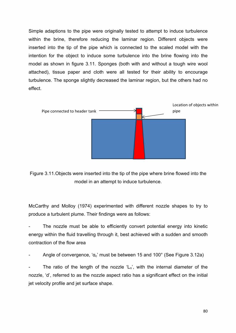
80
Simple adaptions to the pipe were originally tested to attempt to induce turbulence
within the brine, therefore reducing the laminar region. Different objects were
inserted into the tip of the pipe which is connected to the scaled model with the
intention for the object to induce some turbulence into the brine flowing into the
model as shown in figure 3.11. Sponges (both with and without a tough wire wool
attached), tissue paper and cloth were all tested for their ability to encourage
turbulence. The sponge slightly decreased the laminar region, but the others had no
effect.
Figure 3.11.Objects were inserted into the tip of the pipe where brine flowed into the
model in an attempt to induce turbulence.
McCarthy and Molloy (1974) experimented with different nozzle shapes to try to
produce a turbulent plume. Their findings were as follows:
- The nozzle must be able to efficiently convert potential energy into kinetic
energy within the fluid travelling through it, best achieved with a sudden and smooth
contraction of the flow area
- Angle of convergence, ‘αc’ must be between 15 and 100° (See Figure 3.12a)
- The ratio of the length of the nozzle ‘Ln’, with the internal diameter of the
nozzle, ‘d’, referred to as the nozzle aspect ratio has a significant effect on the initial
jet velocity profile and jet surface shape.
Pipe connected to header tank
Location of objects within
pipe

81
- As the ratio of the diameter of the nozzle after contraction ‘d’, with the
diameter of the nozzle before the contraction ‘D’ decreases, the turbulence of the
plume also decreases.
(a) (b)
Figure 3.12.Nozzles with the intent to induce turbulent flow into a fluid exiting the
nozzle. a) nozzle schematic (Source J. McCarthy and A. Molloy 1974), b) Standard
plastic nozzle (Often used with silicone tubes) with similar characteristics to the
nozzle schematic in a).
Figure 3.12 shows that a standard silicone nozzle (b), is similar to the nozzle
schematic (a) produced by McCarthy and Molloy (1974). For the silicone nozzle, D is
substantially larger than d, and there is a smooth contraction. The nozzle was
connected between the pipe and the model, and the laminar region was considerably
reduced. However, when using virtual origin calculations, there is a requirement for
T (see section 2.7.2.6) to be greater than 0.5. When using this nozzle, T is less than
d
D
α
D
d Ln

82
0.5 for all situations where a turbulent plume is produced. As a result, it was deemed
unsuitable.
Hunt and Linden (2001) produced a nozzle designed to generate turbulence within
the brine whilst flowing through the nozzle (see Figure 3.13).This was achieved with
the brine flowing through a 0.1cm diameter opening into a central chamber within the
nozzle and then flowing out of the nozzle through a 0.5cm diameter opening with a
fine mesh across the opening. When the Reynolds number of the brine leaving this
nozzle is 220, the plume was shown to become fully turbulent after a distance of
0.5cm from having nozzle.
Figure 3.13.Nozzle design for inducing turbulence into fluid which allows for virtual
origin corrections. (Source Hunt and Linden (2001)
The outlet of the nozzle contains a fine mesh. To determine which sized mesh was
required to produce a turbulent flow, the nozzle was constructed in three sections,
enabling for access inside the nozzle to change the mesh. Testing of different mesh
sizes within the nozzle proposed is shown in figure 3.14.
Fine mesh

83
(a) (b) (c) (d)
Figure 3.14.Change in laminar region of plume depending on mesh size within
nozzle design used by Hunt and Linden (2001). (a) 40µm mesh, (b) 75 µm mesh, (c)
2 pieces of 75µm mesh on top of each other, (d) 200 µm mesh.
The 200 µm mesh produced the smallest laminar region, with the 40 µm mesh
producing the largest laminar region. Only a small difference was observed between
case (b), with a single piece of 75 µm mesh, and case (c), with two pieces of 75 µm
with a gap between them.
Initially, the nozzles were built in bronze, however this was expensive and time
consuming. Plastic caps (figure 3.15) were used so that ‘mass production’ of the
nozzles was possible, which was important to replace damaged and blocked nozzles.
The internal dimensions of the caps are identical to the dimensions stated in figure
3.13. A 1mm hole was drilled into the top of the cap, and a 1mm thick stainless steel
nut with a 5mm diameter hole at its centre is glued onto the other end of the cap.
The 200 µm mesh is glued between the nut and the cap.
Laminar flow
Laminar flow Laminar flow
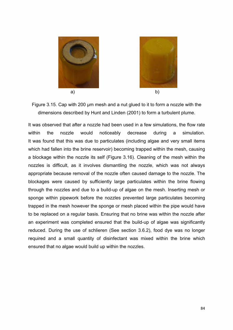
84
a) b)
Figure 3.15. Cap with 200 µm mesh and a nut glued to it to form a nozzle with the
dimensions described by Hunt and Linden (2001) to form a turbulent plume.
It was observed that after a nozzle had been used in a few simulations, the flow rate
within the nozzle would noticeably decrease during a simulation.
It was found that this was due to particulates (including algae and very small items
which had fallen into the brine reservoir) becoming trapped within the mesh, causing
a blockage within the nozzle its self (Figure 3.16). Cleaning of the mesh within the
nozzles is difficult, as it involves dismantling the nozzle, which was not always
appropriate because removal of the nozzle often caused damage to the nozzle. The
blockages were caused by sufficiently large particulates within the brine flowing
through the nozzles and due to a build-up of algae on the mesh. Inserting mesh or
sponge within pipework before the nozzles prevented large particulates becoming
trapped in the mesh however the sponge or mesh placed within the pipe would have
to be replaced on a regular basis. Ensuring that no brine was within the nozzle after
an experiment was completed ensured that the build-up of algae was significantly
reduced. During the use of schlieren (See section 3.6.2), food dye was no longer
required and a small quantity of disinfectant was mixed within the brine which
ensured that no algae would build up within the nozzles.
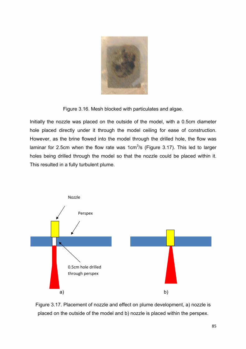
85
Figure 3.16. Mesh blocked with particulates and algae.
Initially the nozzle was placed on the outside of the model, with a 0.5cm diameter
hole placed directly under it through the model ceiling for ease of construction.
However, as the brine flowed into the model through the drilled hole, the flow was
laminar for 2.5cm when the flow rate was 1cm3/s (Figure 3.17). This led to larger
holes being drilled through the model so that the nozzle could be placed within it.
This resulted in a fully turbulent plume.
a) b)
Figure 3.17. Placement of nozzle and effect on plume development, a) nozzle is
placed on the outside of the model and b) nozzle is placed within the perspex.
Nozzle
Perspex
0.5cm hole drilled
through perspex
86
For certain simulations, after steady state was reached, the brine flowing into the
model was turned off. The density throughout the space and the interface height
were then monitored to assess the behaviour of an emptying space. Throughout the
'emptying' phase it was noticed that very small quantities of brine continued to flow
out of the nozzle and into the model. In theory, all the brine within the nozzle and the
piping between the nozzle and the tap which is used to turn off the brine flow into the
model is able to flow into the model. The volume of brine leaking into the model is
small (0.018% of total volume within model). While impossible to completely prevent,
the quantities of brine leaking into the model was deemed sufficiently small to not
have any effect on draining time or alter the draining flow regime.
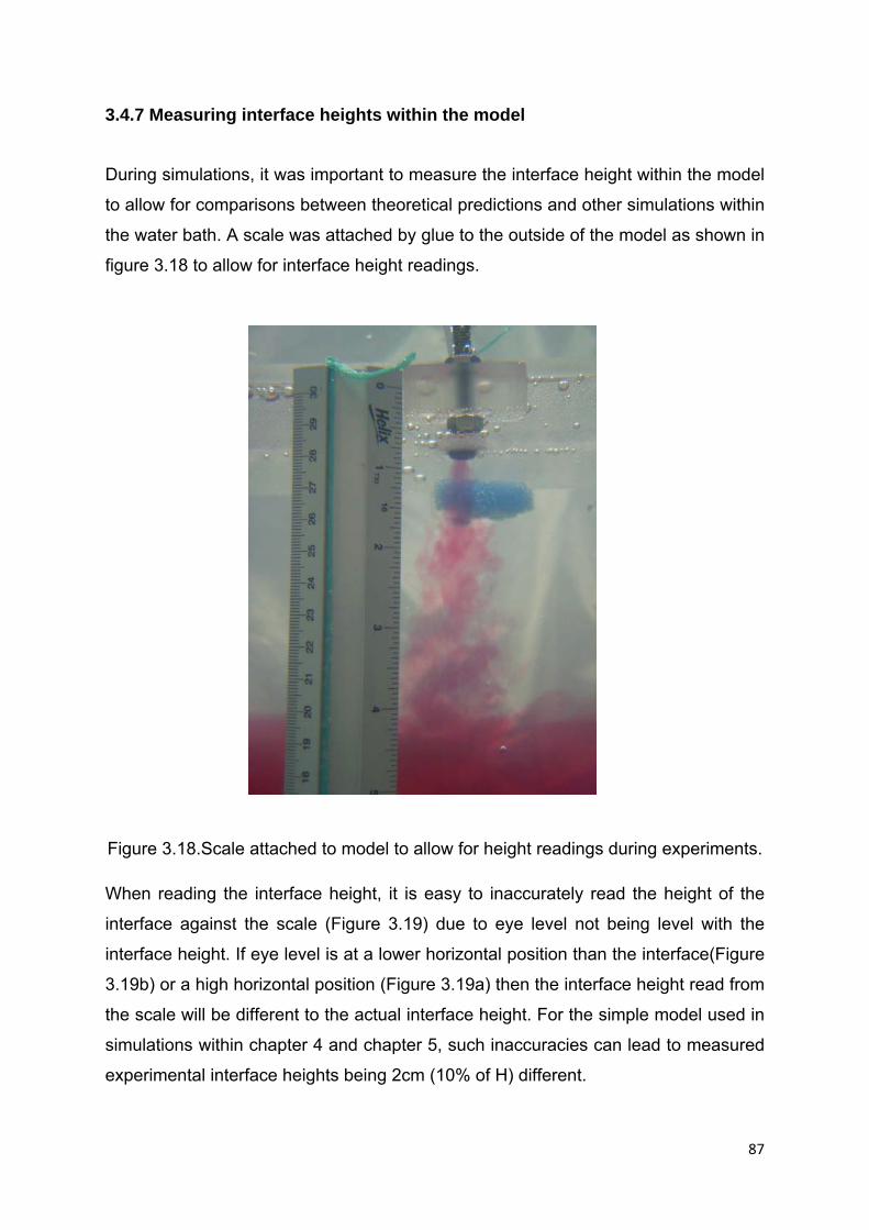
87
3.4.7 Measuring interface heights within the model
During simulations, it was important to measure the interface height within the model
to allow for comparisons between theoretical predictions and other simulations within
the water bath. A scale was attached by glue to the outside of the model as shown in
figure 3.18 to allow for interface height readings.
Figure 3.18.Scale attached to model to allow for height readings during experiments.
When reading the interface height, it is easy to inaccurately read the height of the
interface against the scale (Figure 3.19) due to eye level not being level with the
interface height. If eye level is at a lower horizontal position than the interface(Figure
3.19b) or a high horizontal position (Figure 3.19a) then the interface height read from
the scale will be different to the actual interface height. For the simple model used in
simulations within chapter 4 and chapter 5, such inaccuracies can lead to measured
experimental interface heights being 2cm (10% of H) different.

88
(a) (b) (c)
Figure 3.19. View of brine within model when eye level is (a) above interface height,
(b) below interface height and (c) at interface height level. The top of the brine is
marked in red.
3.5 Density and conductivity measuring devices
Measuring the brine density within the scaled models is important to allow for
comparisons between different opening strategies and with theoretical predictions.
Densities were measured using conductivity probes and a DM-35a density meter.
3.5.1 Anton Parr DM-35a density meter
The DM-35a density meter is a hand held device which collects and dispels samples
by a pump action (Figure 3.20). It has a sensitivity of to 0.001g/cm3 and is able to
store results on its internal memory. The density meter was calibrated using de-
ionised water and was calibrated every week to ensure reliable and accurate density
measurements. It is however not possible to automatically transfer measurements to
a computer as they are taken. The pump action which collects and dispels a sample
can also be quite disruptive which means that it is not appropriate for this density
meter to be used to take density measurements within a reduced scale model during
simulations. This is to avoid the possibility of the collection and dispelling of a sample
causing a change in flow regime or causing mixing across an interface. However, the

89
meter is ideally suited for determining the density of brine in the reservoir tank and to
confirm measurements by the conductivity probes when steady state is reached and
the simulation is about to be stopped.
Figure 3.20. Anton Parr DM-35a density meter used to sample and measure fluid
density.
3.5.2 Conductivity probes.
Conductivity probes were placed within the reduced scale models for the duration of
the simulations. The probes were connected to conductivity meters, which in turn
transferred measured conductivities from the probes in real time to a laptop (Figure
3.21). A measurement was taken every 5 seconds which resulted in a large quantity
of readings throughout the duration of a simulation. For all simulations conducted
within this research, a probe was placed at high level and another at low level.

90
Figure 3.21. Set up of conductivity probes and meters.
The conductivity probes used measured the conductance of the ions present within
the fluid in Siemens (S). Both the type of ion present and their quantity will affect the
conductance, however standard probes are not capable of measuring both the type
of ion and the concentration of the ions present within a fluid, which would allow for
direct conversion into density.
Many equations formed from experimental data are available allowing for the
conversion between conductivity and concentration (Figure 3.22). It should be noted
that the correlation between conductivity and salt concentration is a linear one.
However, each experiment will have different conditions which can affect the
measured conductance, for example the type of fresh water used will have different
quantities of ions present within it even before the salt is added.
.
Conductivity probe
Conductivity meters Laptops
Reduced scale Model
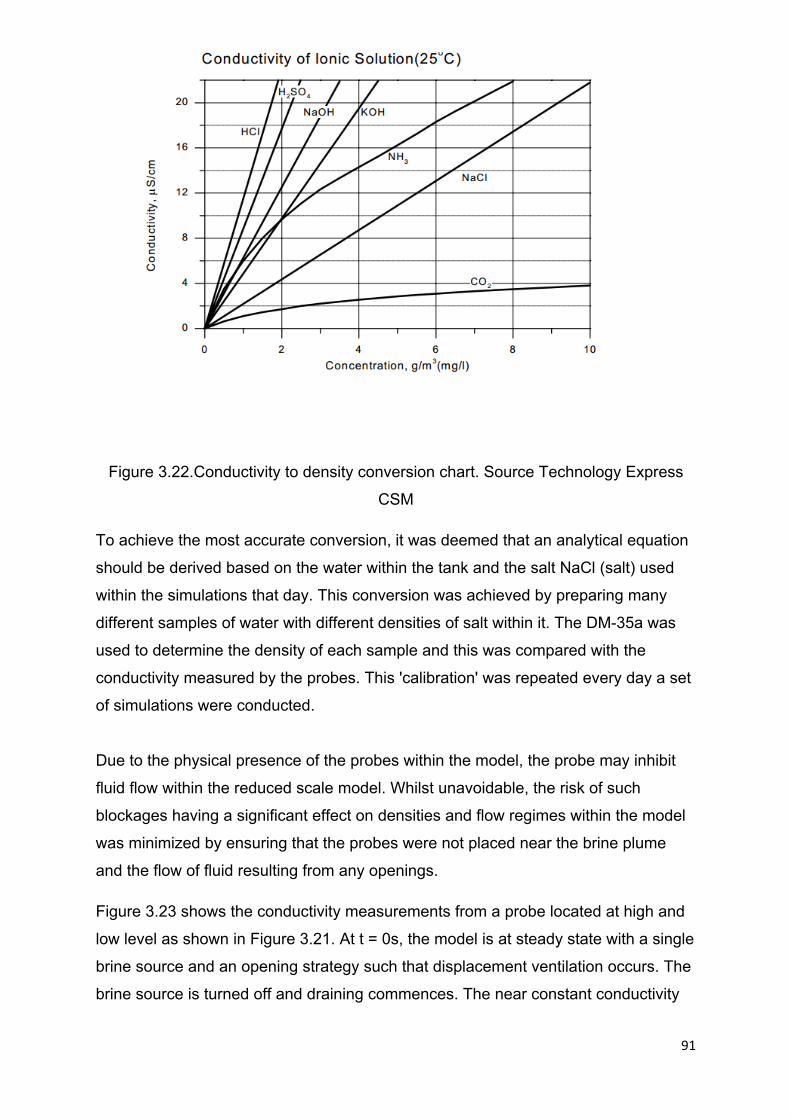
91
Figure 3.22.Conductivity to density conversion chart. Source Technology Express
CSM
To achieve the most accurate conversion, it was deemed that an analytical equation
should be derived based on the water within the tank and the salt NaCl (salt) used
within the simulations that day. This conversion was achieved by preparing many
different samples of water with different densities of salt within it. The DM-35a was
used to determine the density of each sample and this was compared with the
conductivity measured by the probes. This 'calibration' was repeated every day a set
of simulations were conducted.
Due to the physical presence of the probes within the model, the probe may inhibit
fluid flow within the reduced scale model. Whilst unavoidable, the risk of such
blockages having a significant effect on densities and flow regimes within the model
was minimized by ensuring that the probes were not placed near the brine plume
and the flow of fluid resulting from any openings.
Figure 3.23 shows the conductivity measurements from a probe located at high and
low level as shown in Figure 3.21. At t = 0s, the model is at steady state with a single
brine source and an opening strategy such that displacement ventilation occurs. The
brine source is turned off and draining commences. The near constant conductivity
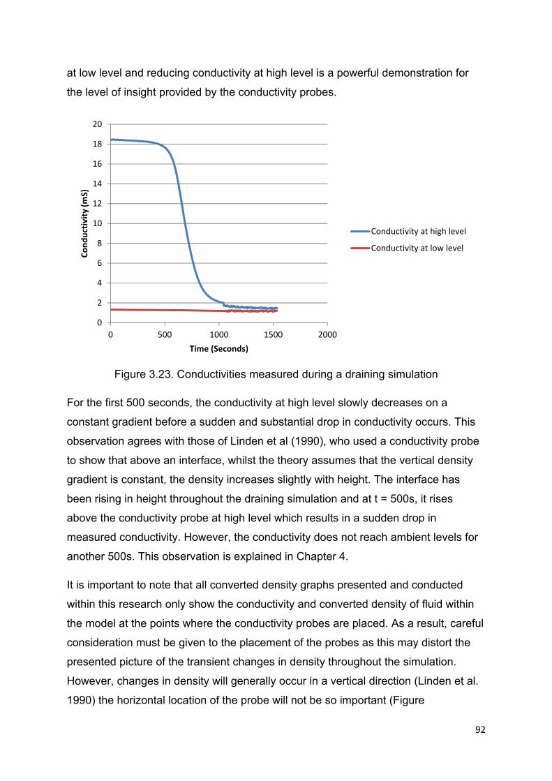
92
at low level and reducing conductivity at high level is a powerful demonstration for
the level of insight provided by the conductivity probes.
Figure 3.23. Conductivities measured during a draining simulation
For the first 500 seconds, the conductivity at high level slowly decreases on a
constant gradient before a sudden and substantial drop in conductivity occurs. This
observation agrees with those of Linden et al (1990), who used a conductivity probe
to show that above an interface, whilst the theory assumes that the vertical density
gradient is constant, the density increases slightly with height. The interface has
been rising in height throughout the draining simulation and at t = 500s, it rises
above the conductivity probe at high level which results in a sudden drop in
measured conductivity. However, the conductivity does not reach ambient levels for
another 500s. This observation is explained in Chapter 4.
It is important to note that all converted density graphs presented and conducted
within this research only show the conductivity and converted density of fluid within
the model at the points where the conductivity probes are placed. As a result, careful
consideration must be given to the placement of the probes as this may distort the
presented picture of the transient changes in density throughout the simulation.
However, changes in density will generally occur in a vertical direction (Linden et al.
1990) the horizontal location of the probe will not be so important (Figure
0
2
4
6
8
10
12
14
16
18
20
0 500 1000 1500 2000
Conductivity (m
S)
Time (Seconds)
Conductivity at high level
Conductivity at low level

93
3.24a).Linden et al. observed horizontal temperature gradients when lower and
upper openings are both located on the same side of a space, resulting in air
temperatures being cooler on the side of the room near the openings (Figure 3.24b).
This results in regions of ‘dead space’ which comprises of a pocket of fluid where
there is little dilution from incoming fresh air. Within a naturally ventilated room, such
regions will likely have higher concentrations of pollutants including CO2 and
temperatures. If occupants inhabit the space where such a region subsides then it
could be detrimental to the health and thermal comfort of the occupant. Dead spaces
were found during initial simulations by the injection of a small amount of dye which
was of a different colour to the dye used within the brine. It was ensured that the
density probes were not located within any dead space areas as this could be
detrimental to the comparison of densities between simulations..
(a) (b)
Figure 3.24. Possible temperature/density gradients within a naturally ventilated
model, (a) vertical gradient and (b) diagonal gradient
For both situations, it is important to consider which probe positions within the model
will provide the most useful data. The placement of probes within this research is
further discussed in the chapters showing the experimental results.
3.6 Photography
Water bath modelling facilitates excellent opportunities for flow visualisation of
transient flows. However, it can be difficult to take a picture or a recording of a flow of
interest within the model, due to camera focussing and the ever changing flow
patterns.

94
The use of screens and lighting was used to improve visualisation of the flow within
the model, which also improves picture and recording quality. However, there is a
limit to the amount that can be captured with traditional techniques. The schleiren
photography technique allows for much more powerful and informative pictures and
recordings, although is quite complex to set up(A. Davidhazy, no date).
3.6.1 Schlieren camera technique
The Schlieren technique uses the principle of light refracting as it travels through
fluids of varying densities to produce shadows on a screen. These shadows
represent areas where light has been refracted due to a change in density.
There are several Schleiren techniques, however, the double pass technique (Figure
3.25) was chosen due to the simplicity of set up, high level of sensitivity to density
change and unlike other Schlieren techniques, it only requires one concave mirror,
which substantially reduces costs (A. Davidhazy, no date). This technique requires a
small light source next to the camera lens, with a concave mirror placed on the far
side of the fluid in question. The high level of sensitivity occurs because light must
travel through the fluid twice before reaching the camera, in effect doubling the
amount of refraction that occurs. The concave mirror reflects the light back towards
the camera and a 6 inch diameter Edmund Scientific concave mirror with a focal
length of 60 inches was used.
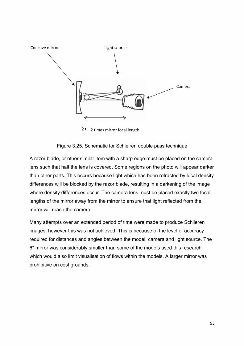
95
Figure 3.25. Schematic for Schleiren double pass technique
A razor blade, or other similar item with a sharp edge must be placed on the camera
lens such that half the lens is covered. Some regions on the photo will appear darker
than other parts. This occurs because light which has been refracted by local density
differences will be blocked by the razor blade, resulting in a darkening of the image
where density differences occur. The camera lens must be placed exactly two focal
lengths of the mirror away from the mirror to ensure that light reflected from the
mirror will reach the camera.
Many attempts over an extended period of time were made to produce Schlieren
images, however this was not achieved. This is because of the level of accuracy
required for distances and angles between the model, camera and light source. The
6" mirror was considerably smaller than some of the models used this research
which would also limit visualisation of flows within the models. A larger mirror was
prohibitive on cost grounds.
Light source Concave mirror
Camera
2 times mirror focal length
Concave mirror Light source
Camera
2 times mirror focal length
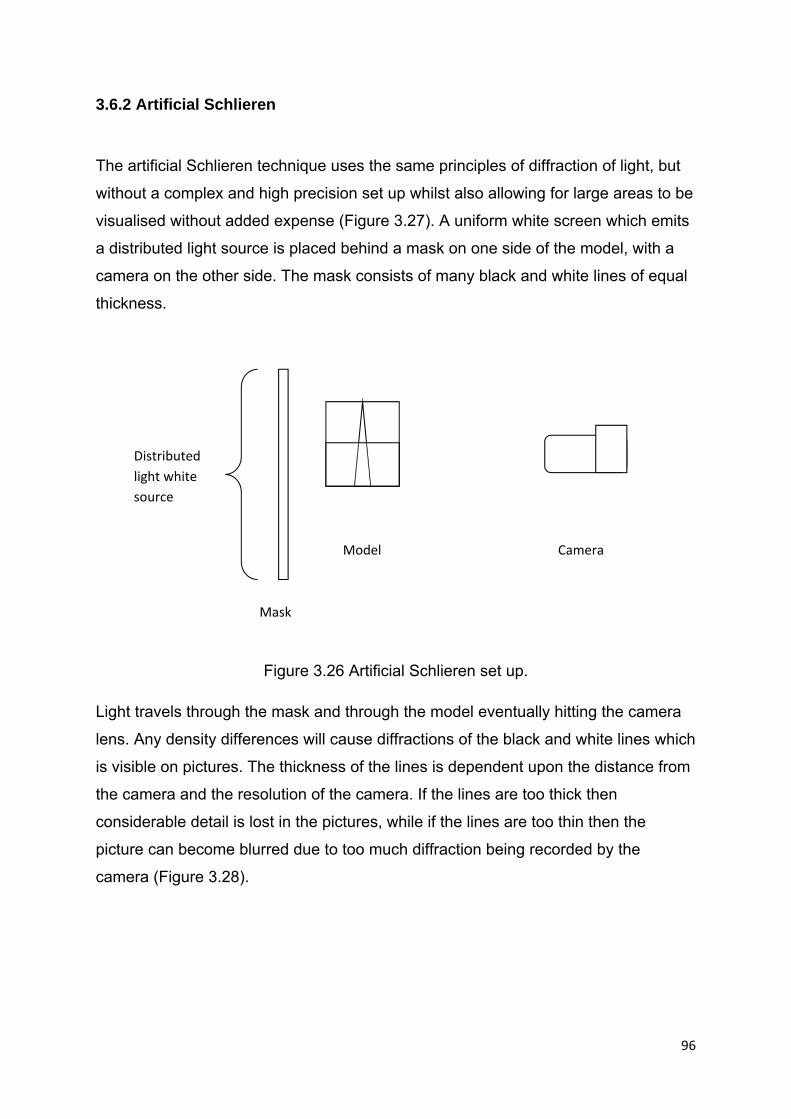
96
3.6.2 Artificial Schlieren
The artificial Schlieren technique uses the same principles of diffraction of light, but
without a complex and high precision set up whilst also allowing for large areas to be
visualised without added expense (Figure 3.27). A uniform white screen which emits
a distributed light source is placed behind a mask on one side of the model, with a
camera on the other side. The mask consists of many black and white lines of equal
thickness.
Figure 3.26 Artificial Schlieren set up.
Light travels through the mask and through the model eventually hitting the camera
lens. Any density differences will cause diffractions of the black and white lines which
is visible on pictures. The thickness of the lines is dependent upon the distance from
the camera and the resolution of the camera. If the lines are too thick then
considerable detail is lost in the pictures, while if the lines are too thin then the
picture can become blurred due to too much diffraction being recorded by the
camera (Figure 3.28).
Mask
Model Camera
Distributed
light white
source
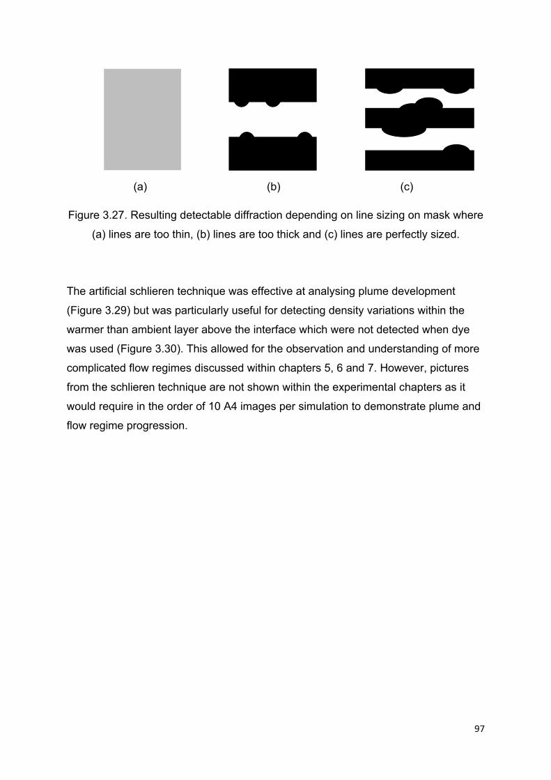
97
(a) (b) (c)
Figure 3.27. Resulting detectable diffraction depending on line sizing on mask where
(a) lines are too thin, (b) lines are too thick and (c) lines are perfectly sized.
The artificial schlieren technique was effective at analysing plume development
(Figure 3.29) but was particularly useful for detecting density variations within the
warmer than ambient layer above the interface which were not detected when dye
was used (Figure 3.30). This allowed for the observation and understanding of more
complicated flow regimes discussed within chapters 5, 6 and 7. However, pictures
from the schlieren technique are not shown within the experimental chapters as it
would require in the order of 10 A4 images per simulation to demonstrate plume and
flow regime progression.

98
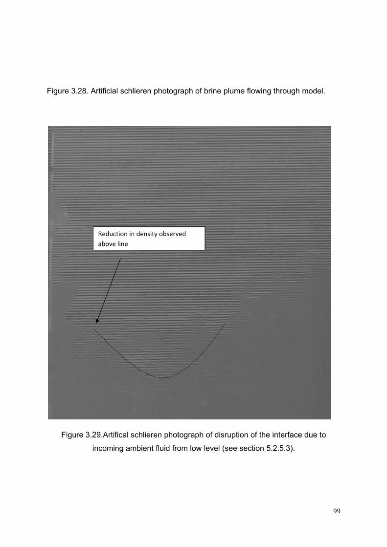
99
Figure 3.28. Artificial schlieren photograph of brine plume flowing through model.
Figure 3.29.Artifical schlieren photograph of disruption of the interface due to
incoming ambient fluid from low level (see section 5.2.5.3).
Reduction in density observed
above line

100
Chapter 4. Benchmark 1 (Simple box) - Validation
4.1 Preamble
This chapter presents the results of experiments conducted using a simple box
which is referred to as Benchmark 1.The results provide validation of the
experimental facility against natural ventilation theory, which includes the effect of
opening area on interface height and internal densities.
4.2 Description of Benchmark 1
Figure 4.1 shows the opening locations, and general geometry of the simple box
model used to validate the water bath facility.
As discussed in chapter 3, the model is inverted, resulting in the heat source being
on the top of the inside of the model. The top of the model is referred to as the floor
and the bottom model is referred to as the ceiling. The model has 4No.2cm diameter
holes located on the floor, 4No.2cm diameter holes and 4No.2.5cm diameter holes
located on the ceiling and 6No. 2cm diameter located on two opposite side walls.
The 4No. 2.5cm diameter holes located on the ceiling are designed to have 2cm
diameter stacks inserted within them. From now on, within the model, high level
refers to an area towards the ceiling and low level refers to an area nearing the floor.
P1 and P2 represent the positions of conductivity probes used to produce converted
density readings. The probe at position P1 is placed 1.5cm above the floor and the
probe at position P2 is placed 1.5cm below the ceiling. Both probes protrude into the
space by 5 cm.
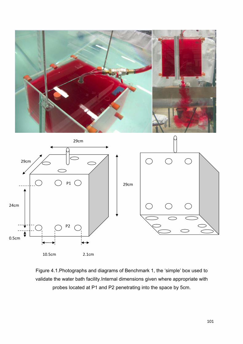
101
Figure 4.1.Photographs and diagrams of Benchmark 1, the ‘simple’ box used to
validate the water bath facility.Internal dimensions given where appropriate with
probes located at P1 and P2 penetrating into the space by 5cm.
TI
SI
SO BO
29cm
29cm
29cm
2.1cm 10.5cm
0.5cm
24cm
P1
P2
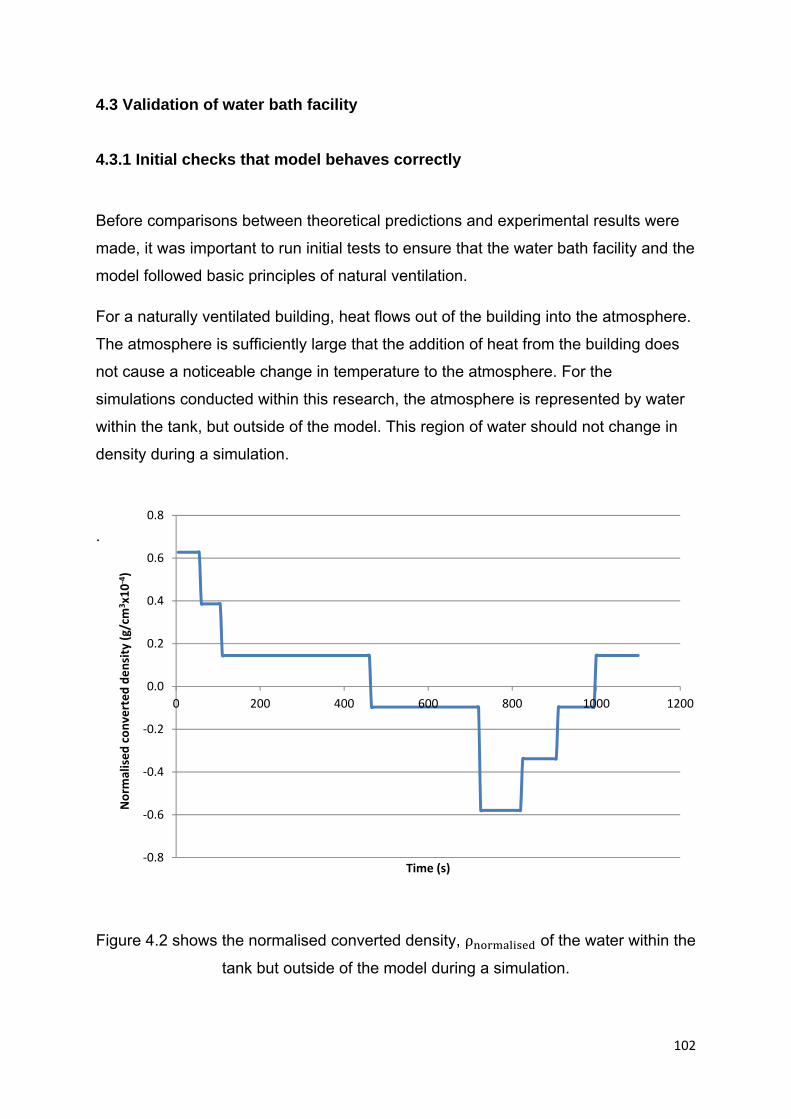
102
‐0.8
‐0.6
‐0.4
‐0.2
0.0
0.2
0.4
0.6
0.8
0 200 400 600 800 1000 1200
Norm
alised converted density (g/cm
3x10‐4)
Time (s)
4.3 Validation of water bath facility
4.3.1 Initial checks that model behaves correctly
Before comparisons between theoretical predictions and experimental results were
made, it was important to run initial tests to ensure that the water bath facility and the
model followed basic principles of natural ventilation.
For a naturally ventilated building, heat flows out of the building into the atmosphere.
The atmosphere is sufficiently large that the addition of heat from the building does
not cause a noticeable change in temperature to the atmosphere. For the
simulations conducted within this research, the atmosphere is represented by water
within the tank, but outside of the model. This region of water should not change in
density during a simulation.
.
Figure 4.2 shows the normalised converted density, ρ of the water within the
tank but outside of the model during a simulation.

103
The normalised converted density is calculated by:
ρ ρ ρ /ρ 4.1
whereρ is the initial density within the model and ρ is the measured converted
density.
Converted densities throughout the 1100 seconds of measurement varied by a
maximum of 1.205 x 10⁻⁴ kg/m3, which is approximately 4000 times smaller than the
change in density that occurred within the model during the simulation. This provides
confidence that the small change in converted density for external ambient water is
due to natural variation within the water and can be assumed to be constant through
simulations.
Densities were also measured during simulations inside the model to ensure that
densities increased from ambient in such a manner to agree with NV theory. Figure
4.3 shows the converted density at high level within a model which is initially filled
with ambient water with openings at both high and low level. When 0 <t< 200s, the
converted density remains constant. At t = 200s, a brine source is turned on within
the model at low level and there is a sudden increase in converted density as the
fluid within the model becomes more dense. At t = 1200s the density stops
increasing and becomes constant with minor fluctuations within 0.05g/cm3. The
thermal environment within the model can be assumed to have reached steady state
at this point in time because the minor fluctuations in density are caused by the
turbulent nature of natural ventilation, which is discussed later in this chapter. The
simulation was run for a further 1500s to show that converted density does not
change once steady state is reached.
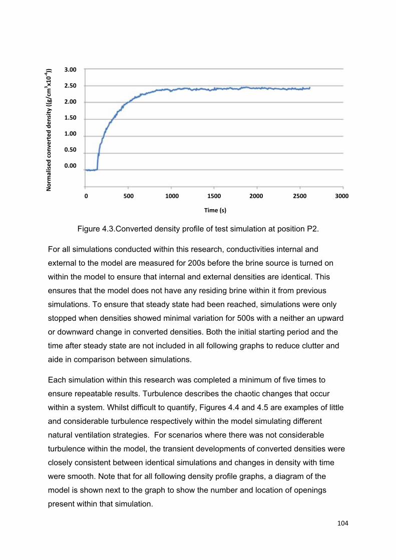
104
Figure 4.3.Converted density profile of test simulation at position P2.
For all simulations conducted within this research, conductivities internal and
external to the model are measured for 200s before the brine source is turned on
within the model to ensure that internal and external densities are identical. This
ensures that the model does not have any residing brine within it from previous
simulations. To ensure that steady state had been reached, simulations were only
stopped when densities showed minimal variation for 500s with a neither an upward
or downward change in converted densities. Both the initial starting period and the
time after steady state are not included in all following graphs to reduce clutter and
aide in comparison between simulations.
Each simulation within this research was completed a minimum of five times to
ensure repeatable results. Turbulence describes the chaotic changes that occur
within a system. Whilst difficult to quantify, Figures 4.4 and 4.5 are examples of little
and considerable turbulence respectively within the model simulating different
natural ventilation strategies. For scenarios where there was not considerable
turbulence within the model, the transient developments of converted densities were
closely consistent between identical simulations and changes in density with time
were smooth. Note that for all following density profile graphs, a diagram of the
model is shown next to the graph to show the number and location of openings
present within that simulation.
Norm
alised
converted den
sity ((g/cm
3x10‐4))
Time (s)
0 500 1000 1500 2000 2500 3000
3.00
2.50
2.00
1.50
1.00
0.50
0.00

105
Figure 4.4 shows the converted density profiles for four simulations with opening
configuration shown in Figure 4.4. Whilst 5No. simulations are conducted, only 4 are
shown to aid in visualisation of all the curves. All 4No.curves are very similar, all
ending at a steady state converted density within 3.3 x10⁻⁵ kg/m3 of each other (0.8%
of the increase from ambient densities to steady state densities). The rates of
increase in density within all five simulations are similar and the time to reach steady
state varies by 25 seconds (approximately 1% of the time to reach steady state). The
near identical density profiles for all 4 simulations suggests minimal turbulence within
the ventilation system.
Figure 4.4. 4No. filling density profiles at P2 with an undisturbed plume.
0.0
0.5
1.0
1.5
2.0
2.5
3.0
3.5
4.0
0 500 1000 1500 2000
Norm
alised converted density ((g/cm
3x10‐4)
Time (s)
1 (P2)
2 (P2)
3 (P2)
4 (P2)
Simulations
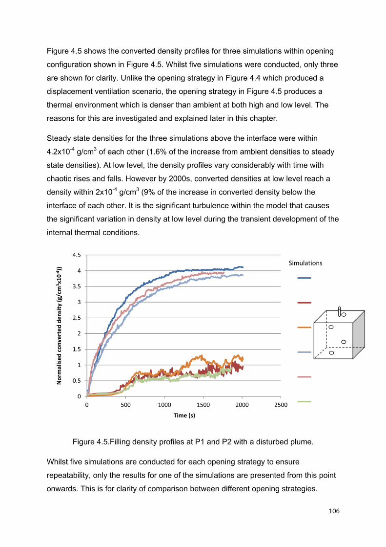
106
Figure 4.5 shows the converted density profiles for three simulations within opening
configuration shown in Figure 4.5. Whilst five simulations were conducted, only three
are shown for clarity. Unlike the opening strategy in Figure 4.4 which produced a
displacement ventilation scenario, the opening strategy in Figure 4.5 produces a
thermal environment which is denser than ambient at both high and low level. The
reasons for this are investigated and explained later in this chapter.
Steady state densities for the three simulations above the interface were within
4.2x10⁻⁴ g/cm3 of each other (1.6% of the increase from ambient densities to steady
state densities). At low level, the density profiles vary considerably with time with
chaotic rises and falls. However by 2000s, converted densities at low level reach a
density within 2x10⁻⁴ g/cm3 (9% of the increase in converted density below the
interface of each other. It is the significant turbulence within the model that causes
the significant variation in density at low level during the transient development of the
internal thermal conditions.
Figure 4.5.Filling density profiles at P1 and P2 with a disturbed plume.
Whilst five simulations are conducted for each opening strategy to ensure
repeatability, only the results for one of the simulations are presented from this point
onwards. This is for clarity of comparison between different opening strategies.
0
0.5
1
1.5
2
2.5
3
3.5
4
4.5
0 500 1000 1500 2000 2500
Norm
alised converted density (g/cm
3x10‐4))
Time (s)
1 (P2)
2 (P1)
3 (P1)
4 (P2)
5 (P2)
6 (P1)
Simulations
107
4.3.2 Experimental and Theoretical comparisons for a draining space.
The theory describing a space initially filled with warmer than ambient air which had
openings such that hot air was flowing out of the model at high level and ambient air
was flowing into the model at low level but has no heat source within it, was
described by Linden et al (1990) and the associated equations 2.1 to 2.10 are in
section 2.7.1. They showed that the water bath technique using brine closely
followed the theory for an emptying space. This section compares the results from
the water bath facility at Loughborough University for draining scenarios with
theoretical predictions. Agreement between theoretical predictions and experimental
results provides confidence in the WBM facility.
4.3.2.1 Methodology for simulating a draining space with classical displacement
Hunt and Coffey (2010 and 2007) and Linden et al (1990) both used water bath
simulations to better understand how the initial interface height, opening area, and
initial internal density within the space affects the time to drain and the flow regime
that occurs whilst draining. In their simulations, the model’s openings were initially
closed and the model was filled with brine of a specific density to a specific height
within the model. Openings at both low and high level were opened at t = 0s.
Simulations following the same methodology are classed as draining methodology 1
(Figure 4.6a). Another set of draining simulations were also conducted and involved
the model being at steady state with low and high level openings and a brine source.
At t = 0s, the brine source is turned off and the model drains. This set of draining
simulations is classed as draining methodology 2 (Figure 4.6b).
During each simulation, the interface height was recorded every 10 seconds. Due to
parallax errors, there was potential for the measured interface height to be incorrect
by up to 10% of H (see 3.4.7). This was minimised by ensuring that eye level was at
a similar level to the interface height, which likely meant that parallax errors were
considerably smaller than 10% of H. However, the maximum potential error in
interface height is shown in Figure 4.7 to demonstrate the potential inaccuracies.

108
Initial t = 0 t > 0 t >> 0
a) Draining methodology1
Initial t = 0 t> 0 t >> 0
b) Draining methodology 2
Figure 4.6.The two different draining methodologies used, i) draining methodology 1
and ii) draining methodology 2.
The reason for conducting draining methodology 2 simulations is to see if the initial
state of the ventilation which would exist in methodology 2 draining simulations but
not in methodology 1 draining simulations had any effect on the draining profile. The
literature review conducted within this research could not find any mention of
experiments following methodology 2.
To ensure that the initial densities within the model for draining methodology 1
draining simulations were homogenous with height, a conductivity probe was slowly
lowered through an inlet, measuring densities throughout the vertical plane of the
model. If densities were not homogenous then a stick was used carefully to mix the
brine. For the scenarios where the model was only partially filled, great care was
taken to ensure that the interface was not disturbed. When draining commenced,
interface heights were measured every minute, which ensured sufficient data plots
and accurate measurements.
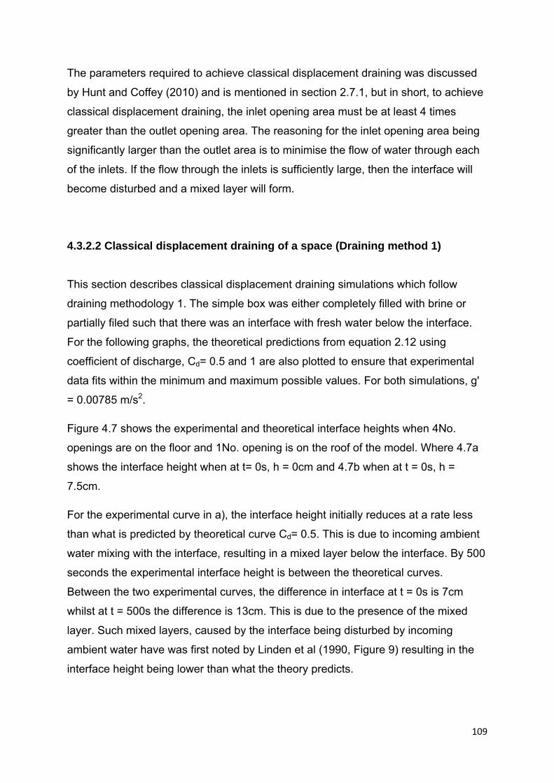
109
The parameters required to achieve classical displacement draining was discussed
by Hunt and Coffey (2010) and is mentioned in section 2.7.1, but in short, to achieve
classical displacement draining, the inlet opening area must be at least 4 times
greater than the outlet opening area. The reasoning for the inlet opening area being
significantly larger than the outlet area is to minimise the flow of water through each
of the inlets. If the flow through the inlets is sufficiently large, then the interface will
become disturbed and a mixed layer will form.
4.3.2.2 Classical displacement draining of a space (Draining method 1)
This section describes classical displacement draining simulations which follow
draining methodology 1. The simple box was either completely filled with brine or
partially filed such that there was an interface with fresh water below the interface.
For the following graphs, the theoretical predictions from equation 2.12 using
coefficient of discharge, Cd= 0.5 and 1 are also plotted to ensure that experimental
data fits within the minimum and maximum possible values. For both simulations, g'
= 0.00785 m/s2.
Figure 4.7 shows the experimental and theoretical interface heights when 4No.
openings are on the floor and 1No. opening is on the roof of the model. Where 4.7a
shows the interface height when at t= 0s, h = 0cm and 4.7b when at t = 0s, h =
7.5cm.
For the experimental curve in a), the interface height initially reduces at a rate less
than what is predicted by theoretical curve Cd= 0.5. This is due to incoming ambient
water mixing with the interface, resulting in a mixed layer below the interface. By 500
seconds the experimental interface height is between the theoretical curves.
Between the two experimental curves, the difference in interface at t = 0s is 7cm
whilst at t = 500s the difference is 13cm. This is due to the presence of the mixed
layer. Such mixed layers, caused by the interface being disturbed by incoming
ambient water have was first noted by Linden et al (1990, Figure 9) resulting in the
interface height being lower than what the theory predicts.
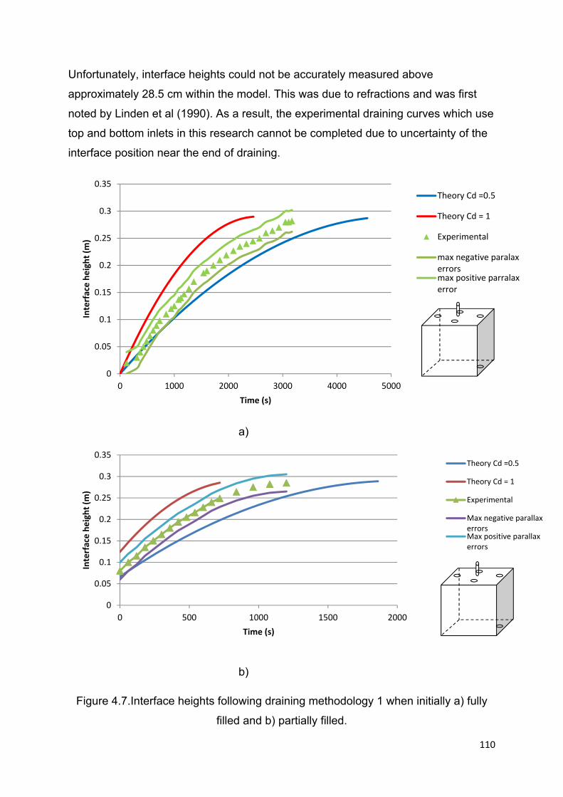
110
Unfortunately, interface heights could not be accurately measured above
approximately 28.5 cm within the model. This was due to refractions and was first
noted by Linden et al (1990). As a result, the experimental draining curves which use
top and bottom inlets in this research cannot be completed due to uncertainty of the
interface position near the end of draining.
a)
b)
Figure 4.7.Interface heights following draining methodology 1 when initially a) fully
filled and b) partially filled.
0
0.05
0.1
0.15
0.2
0.25
0.3
0.35
0 1000 2000 3000 4000 5000
Interface height (m
)
Time (s)
Theory Cd =0.5
Theory Cd = 1
Experimental
max negative paralaxerrorsmax positive parralaxerror
0
0.05
0.1
0.15
0.2
0.25
0.3
0.35
0 500 1000 1500 2000
Interface height (m
)
Time (s)
Theory Cd =0.5
Theory Cd = 1
Experimental
Max negative parallaxerrorsMax positive parallaxerrors

111
Similar simulations except with two outlets on the roof of the model (A* = 6.28 x10-
4m2).Considerable mixing occurred making it impossible to measure interface heights
accurately for the scenario where the model is fully filled. An interface did not form
within the model because there was significant incoming fresh water as predicted by
Hunt and Coffey (2010)and the model was observed to drain with displacement flow
with interfacial mixing. Due to the limited number of openings on the top and bottom
of the model, no more draining simulations could be conducted which ensured
classical displacement with openings on the top and bottom of the model. However,
draining simulations were also conducted using the openings on the side of the
model.
The graphs within Figure 4.7 include the maximum parallax errors which could affect
the interface height reading by + or - 2cm. Whilst significant (10% of H), even with
maximum parallax errors, the interface height readings are within Cd = 1 and 0.5
theoretical curves. Further graphs in this section are plotted with theatrical curve Cd
= 0.61, if the experimental curve closely follows this curve then it can be assumed
that parallax errors were minimal during interface height measurements.
Figures 4.8 and 4.9 show the interface heights whilst draining when the model has
2No.openings on the wall at low and high level and 4 openings on the wall at low and
high level respectively with an initial reduced gravity within the model, g' = 6.44cm/s2.
Li (2000) states that when an opening is on a vertical face like a wall, its midpoint
should be used to represent the height of the opening in all calculations. Because
the model could not be filled with brine beyond the top of the lowest openings as
brine would flow out of the model, the centre of the lower openings was assumed to
also be the lowest point within the model (where H measurements are taken from).
As a result, H = 26cm and when t = 0s, h = 1cm. The theoretical curves using
equation 2.1 were plotted such that at t = 0s, h = 1cm to allow for comparisons
between theoretical predictions and experimental results.
The experimental interface curve for the scenario with 2No.openings at low and high
level is slightly closer to the lower theoretical curve (Cd = 0.61) than the upper
theoretical curve (Cd = 1). The opposite occurs for the scenario with 4No. openings
for the first 200s and can be attributed to a mixed layer forming due to increased F
through the model.

112
.
Figure 4.8. Interface heights during draining following methodology 1.
Figure 4.9.Interface heights during draining following methodology 1 with 4No. side
openings at low and high level.
0
0.05
0.1
0.15
0.2
0.25
0.3
0 200 400 600 800 1000 1200
Interface height (m
)
Time (s)
Theory Cd =0.5
Theory Cd = 1
Experimental
Theory Cd = 0.61
0
0.05
0.1
0.15
0.2
0.25
0.3
0 100 200 300 400 500 600 700
Interface height (m
)
Time (s)
Theory Cd = 0.5
Theory Cd = 1
Experimental
Theory Cd= 0.61

113
Draining simulations both from filled and partially filled positions presented in this
section using draining methodology 1 closely agree with theoretical predictions and
this provides confidence for further draining simulations presented later on within this
research. For simulations with significant F, mixed layers formed as predicted by
Hunt and Coffey (2010). The experimental interface height measurements reported
in this section shows that such mixed layers can cause the interface height to
increase at a slower rate. The literature review for this research found no mention of
how a mixed layer can affect the thermal environment within a space. Mixed layers
and their effects on experimental results will be further discussed in later parts of this
chapter.
4.3.2.3 Classical displacement draining of a space when initially at steady state with a brine source (Draining method 2)
The opening arrangements used in section 4.3.1.2 which had openings on the walls
are repeated using draining methodology 2 with the addition of using the
arrangement with 4No. lower openings and 2No. upper openings. In all cases, a
plume with flow rate = 1cm3/s and density = 1.12g/cm3 was used. The theoretical line
with Cd = 0.61 is also added to allow for comparisons.
For the simulations with side openings (Figures 4.10, 4.11 and 4.12), the
experimental interface height closely follows the theory (when Cd = 0.61) until 25cm.
At this point, the rise in interface height significantly slows in comparison to the
theoretical curves. This slowdown did not occur for the simulations with identical
opening strategies which instead used draining methodology 1 and upon completing
the literature review for this research, no mention of this slowdown was found.
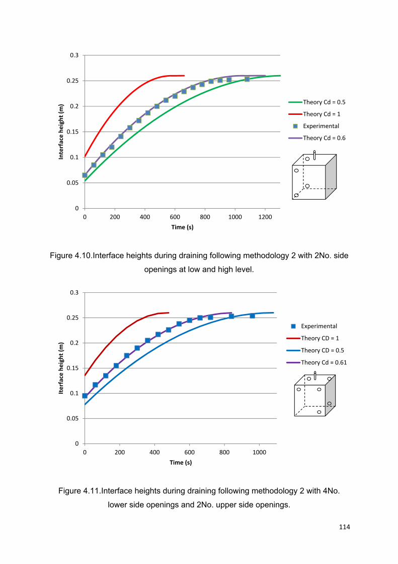
114
Figure 4.10.Interface heights during draining following methodology 2 with 2No. side
openings at low and high level.
Figure 4.11.Interface heights during draining following methodology 2 with 4No.
lower side openings and 2No. upper side openings.
0
0.05
0.1
0.15
0.2
0.25
0.3
0 200 400 600 800 1000 1200
Interface height (m
)
Time (s)
Theory Cd = 0.5
Theory Cd = 1
Experimental
Theory Cd = 0.6
0
0.05
0.1
0.15
0.2
0.25
0.3
0 200 400 600 800 1000
Iterface height (m
)
Time (s)
Experimental
Theory CD = 1
Theory CD = 0.5
Theory Cd = 0.61
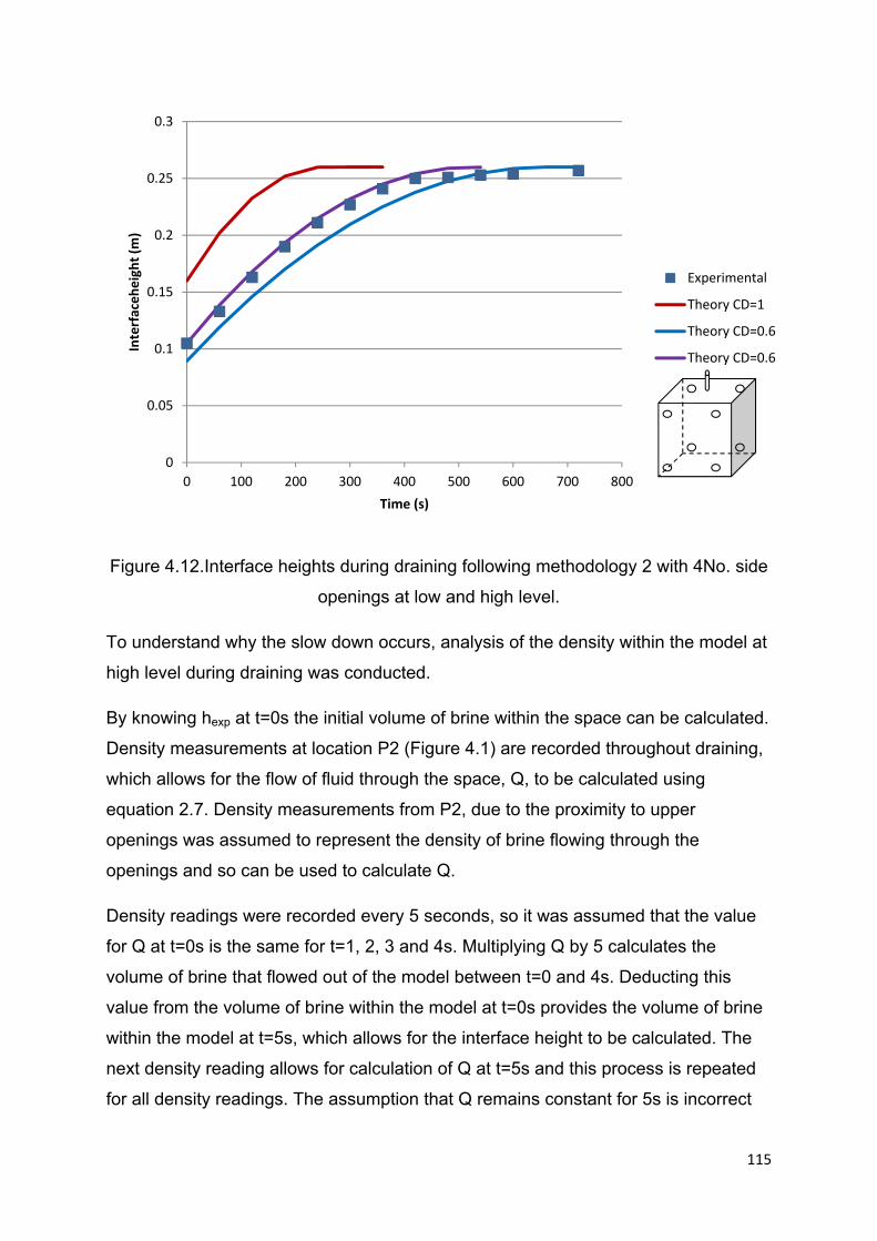
115
Figure 4.12.Interface heights during draining following methodology 2 with 4No. side
openings at low and high level.
To understand why the slow down occurs, analysis of the density within the model at
high level during draining was conducted.
By knowing hexp at t=0s the initial volume of brine within the space can be calculated.
Density measurements at location P2 (Figure 4.1) are recorded throughout draining,
which allows for the flow of fluid through the space, Q, to be calculated using
equation 2.7. Density measurements from P2, due to the proximity to upper
openings was assumed to represent the density of brine flowing through the
openings and so can be used to calculate Q.
Density readings were recorded every 5 seconds, so it was assumed that the value
for Q at t=0s is the same for t=1, 2, 3 and 4s. Multiplying Q by 5 calculates the
volume of brine that flowed out of the model between t=0 and 4s. Deducting this
value from the volume of brine within the model at t=0s provides the volume of brine
within the model at t=5s, which allows for the interface height to be calculated. The
next density reading allows for calculation of Q at t=5s and this process is repeated
for all density readings. The assumption that Q remains constant for 5s is incorrect
0
0.05
0.1
0.15
0.2
0.25
0.3
0 100 200 300 400 500 600 700 800
Interfaceheight (m
)
Time (s)
Experimental
Theory CD=1
Theory CD=0.6
Theory CD=0.6

116
as Q will decrease as the density of the brine flowing through the openings at high
level decreases. This assumption will predict that h is slightly larger than
experimental h because this method assumes a larger volume flowing through the
upper openings than what actually occurs. However the assumption is deemed
adequate for this analysis.
For the scenario where there are 2No. openings at low and high level on the walls,
theoretical interface values calculated in the method described above, theoretical
predictions using Cd = 0.61, experimental h values along with the density recorded at
P2 throughout draining are plotted on Figure 4.13. Whilst theoretical and
experimental interface heights disagree in Figure 4.10 from 23.5cm, close
agreement occurs when the interface height is calculated using experimental
densities.
The theoretical line using Cd = 0.61 assumes that the density throughout the layer of
brine is homogenous. This assumption is applicable to simulations conducted using
draining methodology 1, however it is not applicable to simulations using draining
methodology 2. The density graph in Figure 4.13 shows the density at high level
reducing from approximately 500s. It is at this point that theoretical line using Cd =
0.61 and experimental h recordings begin to differ. Whilst the density at high level
continues to decrease, it is not until 1600s that the model has completely drained.
The decrease in density reduces Q, which causes a reduction in the increase of h.
The prolonged reduced density which is observed in draining methodology 2 does
not occur in draining methodology 1.
The region of prolonged reduced density is actually caused by a mixed layer which
forms below the interface before steady state (t = 0) is reached. This mixed region
causes draining to occur for 300s longer (18%) than the theory predicts. The mixed
region was also experienced in the simulations with openings on the floor and roof of
the model.
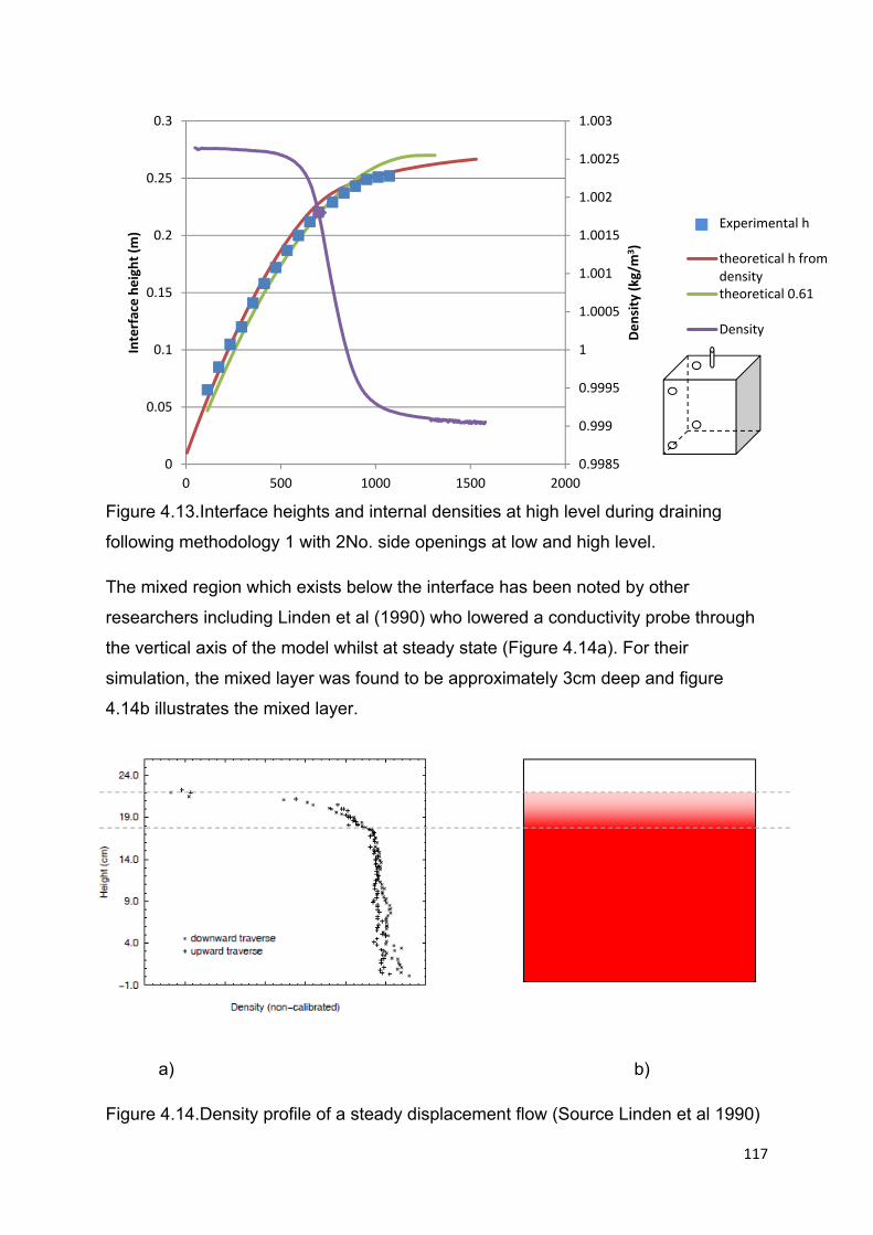
117
Figure 4.13.Interface heights and internal densities at high level during draining
following methodology 1 with 2No. side openings at low and high level.
The mixed region which exists below the interface has been noted by other
researchers including Linden et al (1990) who lowered a conductivity probe through
the vertical axis of the model whilst at steady state (Figure 4.14a). For their
simulation, the mixed layer was found to be approximately 3cm deep and figure
4.14b illustrates the mixed layer.
a) b)
Figure 4.14.Density profile of a steady displacement flow (Source Linden et al 1990)
0.9985
0.999
0.9995
1
1.0005
1.001
1.0015
1.002
1.0025
1.003
0
0.05
0.1
0.15
0.2
0.25
0.3
0 500 1000 1500 2000
Density (kg/m
3)
Interface height (m
)
Experimental h
theoretical h fromdensitytheoretical 0.61
Density

118
The implications of this reduced draining rate could be significant in a NV room, in
particular if a room uses high level openings to allow fresh air to flow into the space
and stale air to flow out of the space (see Chapter 7). For example, if a purging
strategy is designed to remove all excess heat and pollutants from within a space in
between uses, but is unsuccessful due to the reduced draining rate. Such a scenario
would cause high level stale air to mix with fresh incoming air reducing indoor air
quality.
Mixed layers may also be detrimental to thermal comfort of occupants within a space.
This could be particularly true if the NV space relies upon thermal mass to reduce
internal temperatures during the day. This is because thermal mass requires a night
time cooling strategy to reduce its temperature in a process referred to as recharging.
Thermal mass is often placed at high level within a space, usually at ceiling level and
so requires all warm stale air to flow out of the space and cool ambient air to flow
into the space. If a mixed layer is present, the thermal mass within a space will be in
contact with warm air for a longer period of time, reducing its ability to recharge. It is
entirely possible that by the next morning when the space becomes occupied again,
the mixed layer is still present within the space meaning that the thermal mass within
the space is still warm. This will be detrimental to the thermal comfort of a space
during periods of hot weather but may be successful in winter at reducing heating.
4.3.3 Experimental and Theoretical comparisons at steady state
Linden et al (1990) showed that experimental interface heights and densities for a
model simulating a displacement ventilation strategy within a water bath closely
agreed with theoretical predictions at steady state. In this section, the same
comparisons will be conducted to provide further confidence that interface heights
and densities are correctly modelled within the water bath facility.
Whilst there was agreement with density above the interface (Linden et al 1990,
Figure 12b), the experimental interface heights were noted to be lower than the
theoretical heights (Figure 12a). The discrepancy between theoretical and
experimental interface heights was due to virtual origin corrections not being applied.
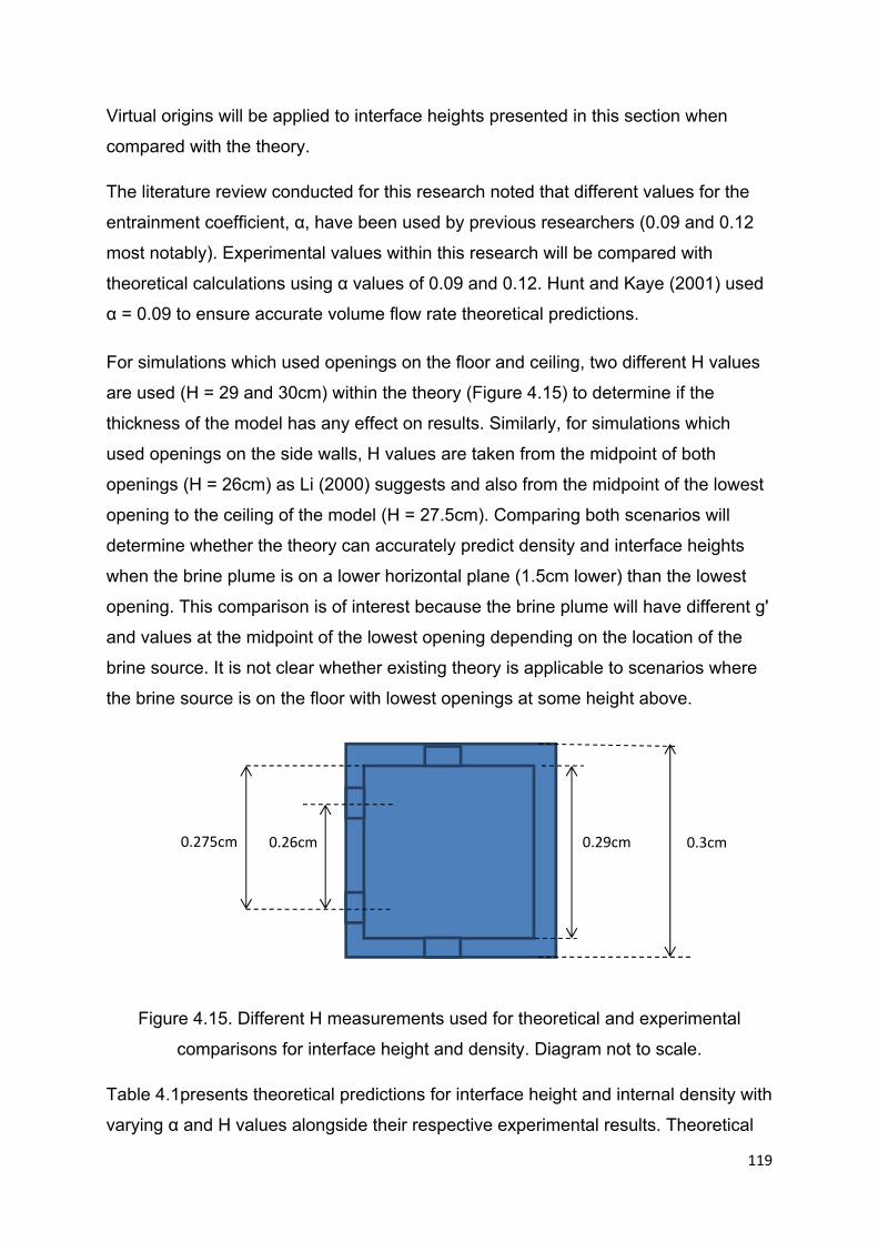
119
Virtual origins will be applied to interface heights presented in this section when
compared with the theory.
The literature review conducted for this research noted that different values for the
entrainment coefficient, α, have been used by previous researchers (0.09 and 0.12
most notably). Experimental values within this research will be compared with
theoretical calculations using α values of 0.09 and 0.12. Hunt and Kaye (2001) used
α = 0.09 to ensure accurate volume flow rate theoretical predictions.
For simulations which used openings on the floor and ceiling, two different H values
are used (H = 29 and 30cm) within the theory (Figure 4.15) to determine if the
thickness of the model has any effect on results. Similarly, for simulations which
used openings on the side walls, H values are taken from the midpoint of both
openings (H = 26cm) as Li (2000) suggests and also from the midpoint of the lowest
opening to the ceiling of the model (H = 27.5cm). Comparing both scenarios will
determine whether the theory can accurately predict density and interface heights
when the brine plume is on a lower horizontal plane (1.5cm lower) than the lowest
opening. This comparison is of interest because the brine plume will have different g'
and values at the midpoint of the lowest opening depending on the location of the
brine source. It is not clear whether existing theory is applicable to scenarios where
the brine source is on the floor with lowest openings at some height above.
Figure 4.15. Different H measurements used for theoretical and experimental
comparisons for interface height and density. Diagram not to scale.
Table 4.1presents theoretical predictions for interface height and internal density with
varying α and H values alongside their respective experimental results. Theoretical
0.26cm 0.275cm 0.29cm 0.3cm
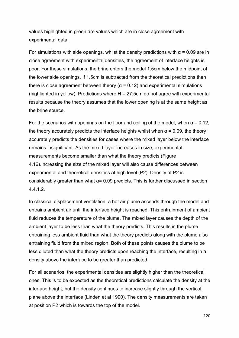
120
values highlighted in green are values which are in close agreement with
experimental data.
For simulations with side openings, whilst the density predictions with α = 0.09 are in
close agreement with experimental densities, the agreement of interface heights is
poor. For these simulations, the brine enters the model 1.5cm below the midpoint of
the lower side openings. If 1.5cm is subtracted from the theoretical predictions then
there is close agreement between theory (α = 0.12) and experimental simulations
(highlighted in yellow). Predictions where H = 27.5cm do not agree with experimental
results because the theory assumes that the lower opening is at the same height as
the brine source.
For the scenarios with openings on the floor and ceiling of the model, when α = 0.12,
the theory accurately predicts the interface heights whilst when α = 0.09, the theory
accurately predicts the densities for cases where the mixed layer below the interface
remains insignificant. As the mixed layer increases in size, experimental
measurements become smaller than what the theory predicts (Figure
4.16).Increasing the size of the mixed layer will also cause differences between
experimental and theoretical densities at high level (P2). Density at P2 is
considerably greater than what α= 0.09 predicts. This is further discussed in section
4.4.1.2.
In classical displacement ventilation, a hot air plume ascends through the model and
entrains ambient air until the interface height is reached. This entrainment of ambient
fluid reduces the temperature of the plume. The mixed layer causes the depth of the
ambient layer to be less than what the theory predicts. This results in the plume
entraining less ambient fluid than what the theory predicts along with the plume also
entraining fluid from the mixed region. Both of these points causes the plume to be
less diluted than what the theory predicts upon reaching the interface, resulting in a
density above the interface to be greater than predicted.
For all scenarios, the experimental densities are slightly higher than the theoretical
ones. This is to be expected as the theoretical predictions calculate the density at the
interface height, but the density continues to increase slightly through the vertical
plane above the interface (Linden et al 1990). The density measurements are taken
at position P2 which is towards the top of the model.

121
The number of simulations was restricted to upper and lower openings where there
was minimal mixing near the interface to allow for accurate interface measurements.
For one of the simulations, the upper opening was reduced in area by 50% to allow
for an additional simulation to be compared within the table.
Opening
arrangement
hexp(m) exp
(kg/m3)
Htheory(m) α htheory(m) theory(kg/m3)

122
0.86-
0.91
1.0025 0.275 0.09 0.128 1.00238
0275 0.12 0.106 1.00213
0.26 0.09 0.126 1.00247
0.26 0.12 0.105 1.00224
0.10 1.002 0.275 0.09 0.138 1.00197
0.275 0.12 0.115 1.00174
0.26 0.09 0.136 1.00206
0.26 0.12 0.113 1.00182
0.117-
0.12
1.0012 0.275 0.09 0.159 1.0013
0.275 0.12 0.133 1.00113
0.26 0.09 0.156 1.001407
0.26 0.12 0.131 1.00119
* 0.082 1.00437 0.3 0.09 0.099 1.00428
0.3 0.12 0.082 1.00393
0.29 0.09 0.098 1.00435
0.29 0.12 0.081 1.0039
0.096 1.0031 0.3 0.09 0.118 1.00287
0.3 0.12 0.098 1.00261
0.29 0.09 0.117 1.00293
0.29 0.12 0.097 1.00266
0.111 1.00161 0.3 0.09 0.144 1.00175
0.3 0.12 0.120 1.00155
0.29 0.09 0.143 1.00180
0.29 0.12 0.119 1.00159
Table4.1.Theoretical and experimental data for interface heights and densities for
different opening arrangements.* refers to the simulation where the upper opening
had its area reduced by 50% to allow for another simulation. Green highlighting
signifies close theoretical and experimental agreement.
Mixed layer
Interface
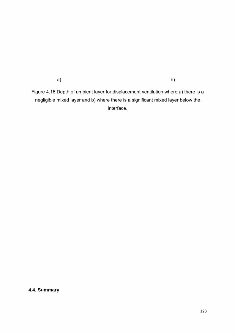
123
a) b)
Figure 4.16.Depth of ambient layer for displacement ventilation where a) there is a
negligible mixed layer and b) where there is a significant mixed layer below the
interface.
4.4. Summary
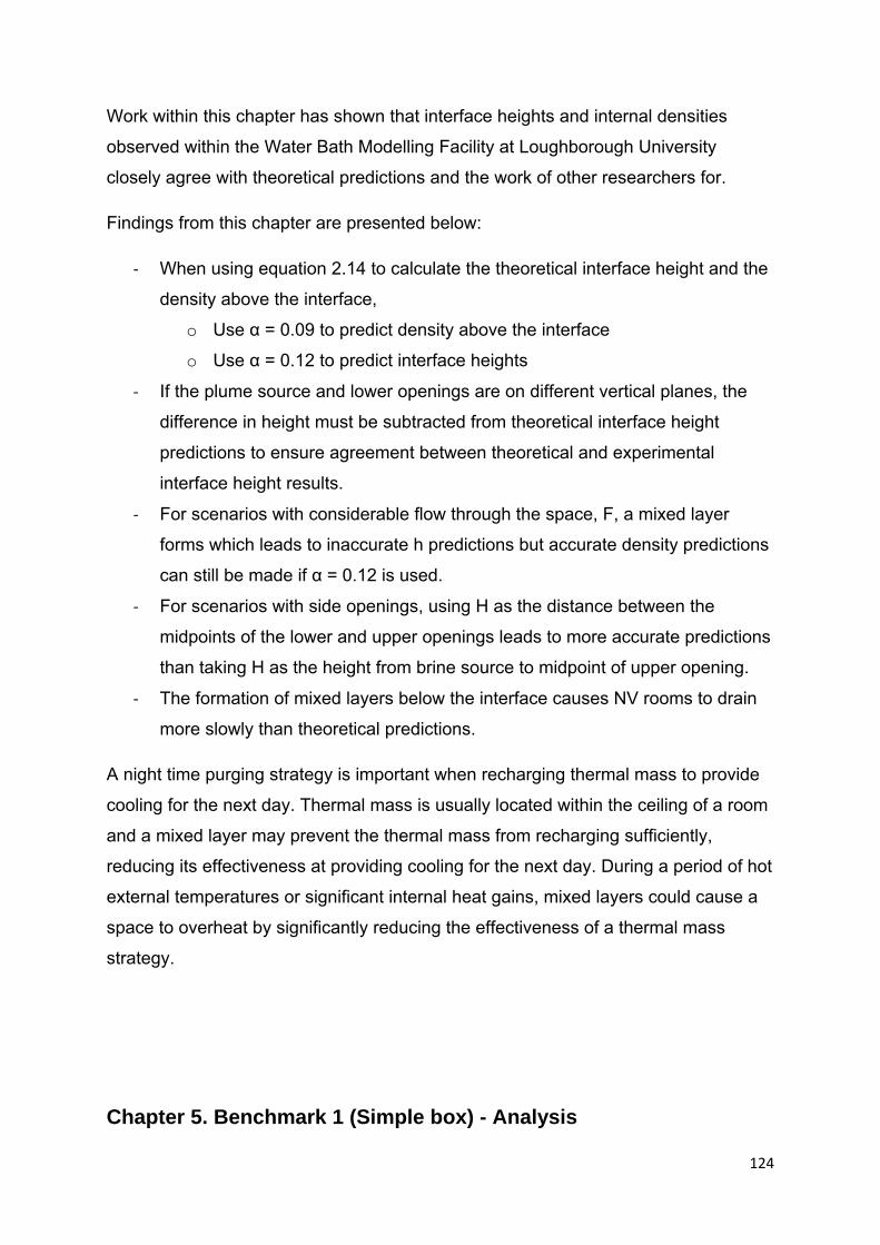
124
Work within this chapter has shown that interface heights and internal densities
observed within the Water Bath Modelling Facility at Loughborough University
closely agree with theoretical predictions and the work of other researchers for.
Findings from this chapter are presented below:
‐ When using equation 2.14 to calculate the theoretical interface height and the
density above the interface,
o Use α = 0.09 to predict density above the interface
o Use α = 0.12 to predict interface heights
‐ If the plume source and lower openings are on different vertical planes, the
difference in height must be subtracted from theoretical interface height
predictions to ensure agreement between theoretical and experimental
interface height results.
‐ For scenarios with considerable flow through the space, F, a mixed layer
forms which leads to inaccurate h predictions but accurate density predictions
can still be made if α = 0.12 is used.
‐ For scenarios with side openings, using H as the distance between the
midpoints of the lower and upper openings leads to more accurate predictions
than taking H as the height from brine source to midpoint of upper opening.
‐ The formation of mixed layers below the interface causes NV rooms to drain
more slowly than theoretical predictions.
A night time purging strategy is important when recharging thermal mass to provide
cooling for the next day. Thermal mass is usually located within the ceiling of a room
and a mixed layer may prevent the thermal mass from recharging sufficiently,
reducing its effectiveness at providing cooling for the next day. During a period of hot
external temperatures or significant internal heat gains, mixed layers could cause a
space to overheat by significantly reducing the effectiveness of a thermal mass
strategy.
Chapter 5. Benchmark 1 (Simple box) - Analysis

125
5.1 Preamble
This chapter presents the results of experiments conducted using a simple box
which is identical to that used in Chapter 4.Whilst Chapter 4 validated the Water
Bath Modelling Facility, Chapter 5 analyses the effect that different ventilation
strategies have on internal temperatures, interface heights and flow regimes. The
results from these simulations allows for an assessment of the effectiveness of
different opening strategies at achieving comfortable internal temperatures and fast
draining times during cooler external temperatures (e.g. winter) and warmer external
temperatures (e.g. summer).
5.2 Filling comparisons of note
Sections 5.2 and 5.3 describe simulations which were conducted to compare flow
regimes, densities and interface heights with the findings of other researchers and
theoretical predictions. Close agreement was observed which provides confidence
that the water bath modelling facility at Loughborough University closely simulates
natural ventilation in buildings. This confidence allows for more complicated
investigations into NV strategies to be conducted.
Fitzgerald and Woods (2008) investigated the effect that varying the position of the
lower and upper openings had on the thermal environment within their water bath
modelling simulations (See chapter 2.8.2). The effect of opening locations is further
investigated in this section with an emphasis on investigating the effectiveness of
different ventilation strategies at providing ventilation to a space.
Filling density profiles are analysed for a wide range of opening areas and strategies
to analyse the effect on flow regimes and densities throughout the model. Initially,
density profiles for simulations using the same ventilation strategy, but with different
opening areas are compared. Towards the end of this chapter, density profiles are
compared between different opening strategies with the same opening area. Such
comparisons may help future NV building designers to select appropriate NV
126
strategies based on the flow regimes and densities that they believe would make the
occupants most comfortable.
For all simulations, at t = 0s, the model is filled only with ambient water and the brine
source is turned on. Using scaling methods from chapter 3, the brine source in all
simulations conducted in this section simulates a 50W heat source.
5.2.1 Geometries with side inlets and outlets
Density profiles from simulations using side openings only are discussed and
compared in this section. Simulations are divided into two types and compared
separately:
‐ The brine plume is not disturbed leading to displacement ventilation.
‐ The brine plume is disturbed by incoming fresh fluid leading to mixed layer
ventilation
The brine plume becomes disturbed when a specific opening at low level is used as
discussed in 4.4.3.
5.2.1.1 Geometries without a disturbed heat source
Figure 5.1 shows the density profile from a conductivity probe placed at P2 for
simulations with openings on opposing side walls at low and high level. Simulation a)
has 4No. openings at low and high level, whilst b) has 2No. openings, c) has 2No. at
low level and 4No. at high level and d) has 4No. at low level and 2No. at high level.
Throughout the simulations, the probe at P1 recorded densities which varied by
1x10⁻⁷ kg/m3 (0.0001% of the density difference measured in simulations) throughout
all simulations and is comparable to measurements taken within the tank but outside
of the model. In all four cases, the density increases at the same rate with time up
until approximately 100 seconds. At this point in time, the density within the
simulation which had 4No.openings at high and low level increased at a reduced rate
to the other three simulations. After 500 seconds, the density within the two
127
simulations which had 2No. and 4No. openings at high and low level increased at a
reduced rate compared with the simulation with 2No. openings at high and low level.
Figure 5.1.Filling simulations with openings on the walls at low and high level
positioned such to ensure an un-disturbed plume, where density profiles are at high
level and low level.
Whilst simulations c) and d) can be described as being half way in between
simulations a) and b) with regards to number of openings, however densities at
steady state and time to reach steady state are closer to those of simulation b) than
simulation a). This agrees with Equation 2.8 which states that if there is a difference
in area between upper and lower openings, the smaller area will mostly determine
interface heights and flow through the space.
5.2.1.2 Geometries with a disturbed heat source plume
0
0.5
1
1.5
2
2.5
3
3.5
4
0 500 1000 1500
Norm
alised converted density
Time (s)
4SI 4SO
2SI 2SO
4SI 2SO
2SI 4SO
a)
b)
c)
d)
Simulations

128
Simulations investigated in 5.2.1.1 used only 4No. of the available 6No. side
openings at high and low level. The opening which was not used is located half way
across the wall (Figure 5.2). The location causes incoming fresh water to collide with
the brine plume which causes the thermal environment within the model to vary from
a traditional stratified state which occurs under displacement ventilation. Such a
collision occurs in all simulations described in this section and density profile graphs
show measured densities at both P1 (low level) and P2 (high level).
a) b)
Figure 5.2.The side openings in line with the location of the plume with a) and b)
showing different side view points.
Figure 5.3 presents the density filling profiles at P1 and P2 during three filling
simulations for the opening strategies with openings placed on opposing side walls
at low and high level. Simulation a) has 4No. openings placed at low and high level,
b) has 2No. and c) has 6No. At high level, densities follow a similar trend to that
described in 5.2.1.1. However, at low level, densities increase beyond ambient.
For all three simulations, densities at low level remain at ambient density until 230s
(simulation b), 400s (Simulation a) and 450s (simulation c) at which point densities
begin to rise. The rate of increase in density is greatest for simulation c)
(0.0017kg/m3 increase from ambient when steady state is reached) and is smallest
for simulation a) (0.0001kg/m3 increase from ambient when steady state is reached).
An increase in density at low level suggests that for this ventilation strategy, there

129
will be a warming of the air at low level. This could be desirable for scenarios where
incoming ambient air is cold and would cause thermal discomfort with droughts
which is of particular use during winter. Whilst incoming ambient water collides with
the brine plume during all three simulations, the time for densities at low level to
increase and the extent that they increase by vary between the three simulations.
Figure 5.3.Filling simulations with openings on the walls at low and high level
positioned such to ensure a disturbed plume, where density profiles are at high level
and low level.
An interface was observed during all three simulations, with a mixed layer below the
interface which formed due to incoming ambient fluid colliding with the plume (Figure
5.4). When brine first starts flowing into the space, a high level interface forms and
slowly decreases in height. At the same time the density of the brine above the
interface increases resulting in increased volume flux, F throughout the space. This
increased flow causes the ambient fluid flowing through the lower opening to have
an increased velocity resulting in increased penetration of ambient fluid through the
space. At some point in time, the penetration is such that the incoming ambient fluid
collides with the plume causing it to partially lose its conical structure and begin
oscillating side to side. However it should be noted that F was not large enough
0
0.5
1
1.5
2
2.5
3
3.5
4
4.5
0 500 1000 1500 2000 2500
Norm
alised converted density
Time (s)
1
2
3
4
5
6
a)
b)
c)
Simulations

130
within the simulations conducted to cause the plume to completely lose its shape.
The plume was observed during simulations to expanding in size with height, this
was likely due to a mix of entrainment and the collision with incoming fluid.
A degree of mixing occurs during the collision resulting in an increase in density of
the area below the interface. As F increases throughout a simulation until steady
state, the resulting collision increases the deformation of the conical structure of the
plume and further increases the density below the interface with increased mixing.
As the density at low level increases, the incoming fresh fluid obtains increased
density before the collision with the plume. At the same time, the increase in density
at low level also reduces buoyancy of the plume lost due to entrainment because the
plume is entraining fluid of increased density. Both of these factors results in the
plume carrying additional buoyancy when penetrating the interface compared with
the simulations conducted in 5.2.1.1 with undisturbed plumes. Upon steady state
being reached, the simulations with disturbed heat sources achieves greater
densities than the simulations without a disturbed heat source.
a) t/tss=0.1 b) t/tss= 0.5 c) t/tss = 1
Figure 5.4. Disturbance of brine plume with time during a simulation

131
5.2.1.3 Geometries with openings on the floor and ceiling
Within this section, density profiles are compared for simulations which have
openings on the floor and ceiling of the model (Figure 5.5). Simulation a) consists of
4No. openings at low and high level, b) consists of 3No. c) consists of 2No. and d)
consists of 1No.
Initially, as brine flows into the model, traditional displacement ventilation occurs with
a layer of brine at high level increasing in depth. However for the 4No.simulations,
the layer of ambient density below the interface begins to gain density in the region
of 350-500s.
Steady state is reached at 600, 800, 1500 and 1700 seconds for simulation a), b), c)
and d) consecutively (Figure 5.5).
The manner in which densities at P1 increase is significantly different to scenarios
with side openings which include the middle inlet. There is a small but gradual
increase in density between 200 and 500 seconds at which point the densities
increase very quickly. Time to reach steady state at P1 is also longer than at the P2
within the model, with times 1100, 1250, 1500 and 1900 seconds for simulations a),
b), c) and d) consecutively.
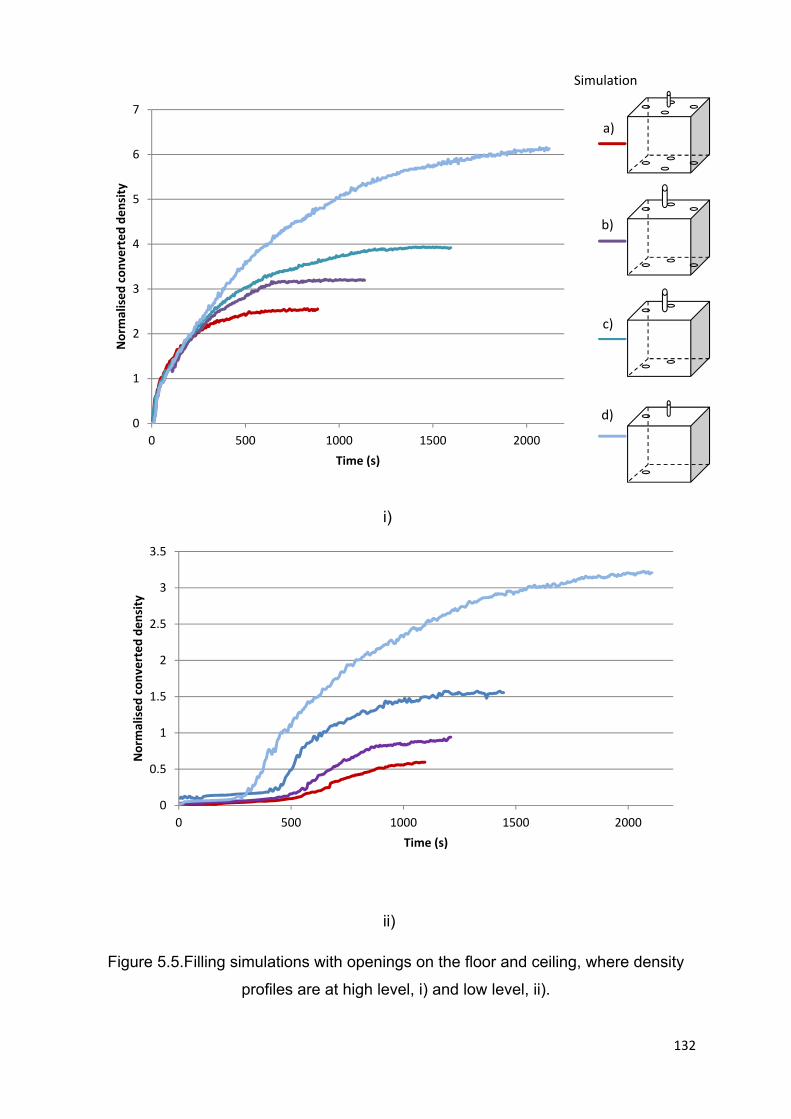
132
0
0.5
1
1.5
2
2.5
3
3.5
0 500 1000 1500 2000
Norm
alised converted density
Time (s)
i)
ii)
Figure 5.5.Filling simulations with openings on the floor and ceiling, where density
profiles are at high level, i) and low level, ii).
0
1
2
3
4
5
6
7
0 500 1000 1500 2000
Norm
alised converted density
Time (s)
4TI:4BO
3TI:3BO
2TI:2BO
1TI:1BO
a)
b)
c)
d)
Simulation

133
The reason why displacement ventilation does not occur when openings are located
on the floor and ceiling while having equal opening areas at steady state is explained
in Figure 5.6.
The blue triangle used within Figure 5.6i represents the plume of ambient fluid
flowing into the space while the red triangle represents the hot air plume resulting
from a heat source. A shade of red is used to represent the extent than an area has
observed an increase in temperature from ambient temperature. Internal
temperatures and F both increase throughout the simulation until steady state, the
penetration of ambient fluid through the lower openings increases. Internal
temperatures increase throughout the duration of the simulation until steady state is
reached which causes F to also increase until steady state is reached. As F
increases, the incoming ambient air has an increased velocity associated with it,
resulting in the incoming ambient air penetrating further into the space. F becomes
sufficiently large that the incoming ambient air collides with the interface and
penetrates into the region of warmer than ambient air and results in the ventilation
strategy becoming disturbed. This disturbance was noted in 4.3.1.2 however
because the lower opening area is equal to the upper opening area, the penetration
is sufficient such that the space becomes filled with brine. The density profile of such
scenarios is discussed in 5.4.3 however, above the point where there is penetration
of ambient fluid, the density is reasonably constant and below this point, the density
decreases the closer fluid is to the floor.
Figure 5.6ii is a photo of a simulation within the WBM facility taken at t=250s.
Incoming fresh water at openings within the floor can be observed to penetrate
through the interface, creating conical shapes within the denser than ambient region.
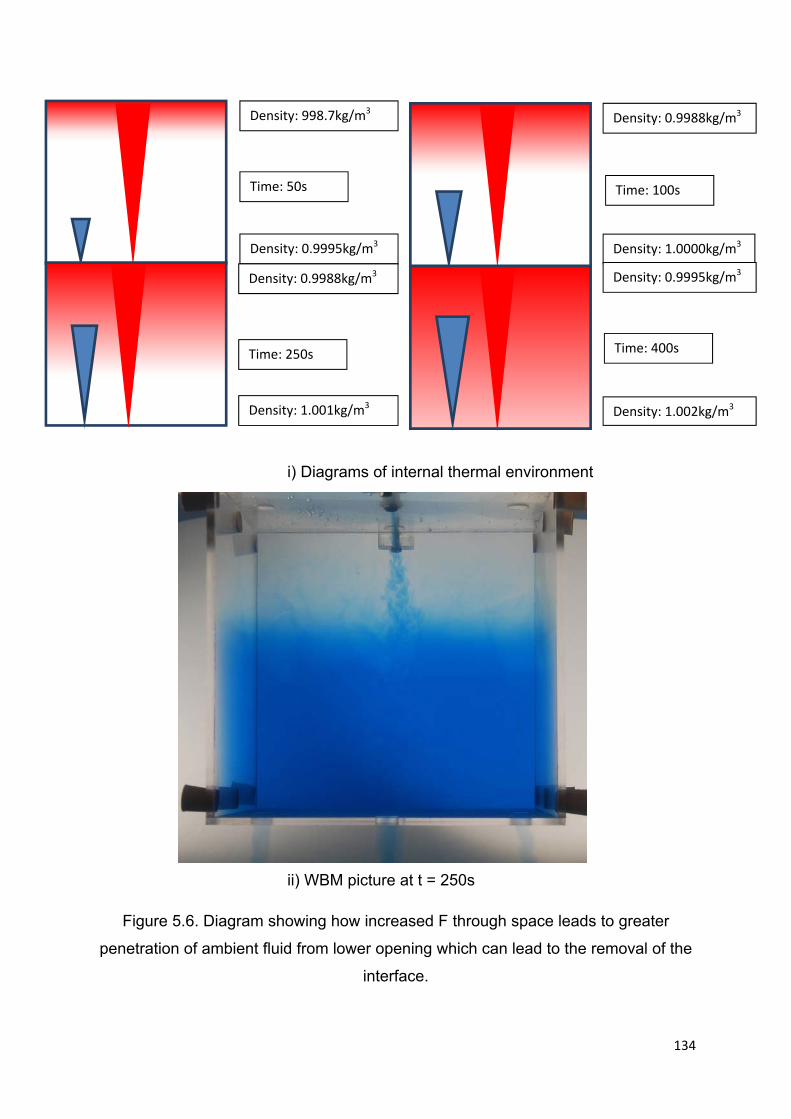
134
i) Diagrams of internal thermal environment
ii) WBM picture at t = 250s
Figure 5.6. Diagram showing how increased F through space leads to greater
penetration of ambient fluid from lower opening which can lead to the removal of the
interface.
Density: 998.7kg/m3
Density: 0.9995kg/m3
Time: 50s
Density: 0.9988kg/m3
Density: 1.0000kg/m3
Time: 100s
Density: 0.9988kg/m3
Density: 1.001kg/m3
Time: 250s
Density: 0.9995kg/m3
Density: 1.002kg/m3
Time: 400s
135
Using equation 2.3, it is possible to calculate Q (and therefore the speed) of
incoming ambient fluid into the space by using equation 2.3. Table 5.2 shows the
times at which density increases beyond ambient are recorded at low level within the
model. Interestingly, when an increase in density from ambient density at low level
occurs for all four simulations, the flow rate and therefore the speed of incoming
ambient fluid through each of the openings into the model for all four simulations is
25.1cm3/s and 10.8cm/s respectively (Table 5.2). For example, when density at low
level is measured to increase beyond ambient, simulation a) which has 4No.
openings at low and high level has a flow rate through the model, Q, of 100.4cm3/s
whilst simulation c) which has 2No. openings has a flow rate through the model of
50.2cm3/s. This means that the flow through each opening, Qopening and the velocity
of fluid through each opening, Uopening for each of the four simulations when densities
at low level increases from ambient are identical.
Table 5.2. Speed of incoming ambient fluid into the model when disruption to
interface occurs with openings on the floor and ceiling of the model.
Simulation a b c d
t (s) 175 190 210 225
(g/cm3) (density at probe 1) 1.00075 1.000764 1.000726 1.000721
Qper opening (using equation 2.3)
(cm3/s)
25.1 25.1 25.1 25.1
Uper opening (cm/s) 10.7 10.8 10.8 10.8
However, it is only in the interval between 340 and 505s that the rate of increase in
density significantly increases between the four simulations at low level and as such,
Table 5.3 shows the speed of incoming fluid during this time. Unlike in Table 5.2
where all four simulations had similar densities at high level resulting in near identical
speeds, there is more variation. Densities and interface heights vary between all four
simulations at the point at which significant disruption of the interface occurs. This
closely agrees with the findings of Hunt and Coffey (2010) who showed that
increasing the incoming velocity or decreasing the density of the stratified layer
would both lend towards disruption of the interface, resulting in a mixed internal
environment.
136
As the number of openings at low and high level decreases, the density above the
interface increases, therefore the incoming fluid velocity requires a greater U to be
able to disrupt and penetrate the interface. However, the requirement for increased
fluid velocity is partially offset by the decreasing interface height due to reduced
openings. This is demonstrated by Table 5.3, which shows simulation d) with the
highest U and highest density above the interface, but also has the lowest h due to
having the smallest number of upper and lower openings. This is in comparison with
simulation a), which has the lowest U, lowest density above the interface with the
highest h. The results suggest that interface height plays a less significant role than
density above the interface for determining when significant disruption occurs.
Table 5.3.Speed of incoming fluid through when significant disruption to interface
occurs with openings on the floor and ceiling.
a b c d
t (s) 505 425 370 340
(g/cm3) (density at probe upper
probe)
1.0012 1.00143 1.001562 1.001605
Qper opening (using equation 2.3)
(cm3/s)
16.14 17.14 17.55 17.68
Uper opening (cm/s) 11.8 12.4 12.7 12.9
5.2.2. Geometries with bottom inlets and top stack outlets
Figure 5.7 shows the density profile for scenarios where openings are located on the
floor and stacks extrude from the ceiling. Simulation a) consists of 1No. openings at
low and high level, b) 2No. openings, c) 3No. openings and d) 4No. openings.
Steady state is reached at 1500, 1300, 1100 and 1000s for simulations a), b), c) and
d) consecutively.
The way the brine builds up in this region is identical to the scenario with openings
on the floor and ceiling without stacks discussed in 5.4.2.
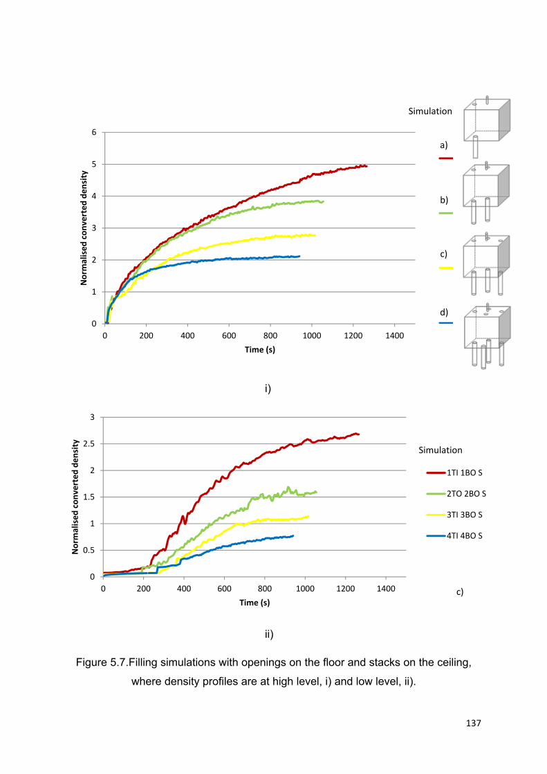
137
0
0.5
1
1.5
2
2.5
3
0 200 400 600 800 1000 1200 1400
Norm
alised converted density
Time (s)
1TI 1BO S
2TO 2BO S
3TI 3BO S
4TI 4BO S
Simulation
i)
ii)
Figure 5.7.Filling simulations with openings on the floor and stacks on the ceiling,
where density profiles are at high level, i) and low level, ii).
0
1
2
3
4
5
6
0 200 400 600 800 1000 1200 1400
Norm
alised converted density
Time (s)
a)
b)
c)
d)
c)
Simulation

138
Density filling profiles at low level follows the same trend as noted in 5.4.2 where
there is a small increase in densities until a certain time at which point densities at
low level begin to increase at a much faster rate. Mean inlet velocity calculations are
conducted in the same manner as in section 5.4.2.
Table 5.4 shows mean velocities for all four simulations at the moment an increase
in density at low level is noted. There is a variance of 0.2cm/s between the four
simulations which is comparable to 0.1cm/s noted in table 5.2.
The stack plays a significant role in increasing flow through the space (see equation
2.3 and 2.4), which results in larger flow speeds for the incoming fresh fluid, which
results in increased penetration. This causes the interface to become disrupted
much earlier in the simulation than experienced in the simulations without stacks. As
a result, U in table 4.5 is approximately 3cm/s faster than U for the case without
stacks.
Table 5.4.Speed of incoming fluid through when disruption to interface occurs with
openings on the floor and stacks on the ceiling.
a b c d
t (s) 90 100 105 115
(g/cm3) (density at probe 1) 1.000304 1.000344 1.00033 1.000328
Qper opening (using equation 2.3)
(cm3/s)
31.1 31.5 31.3 31.3
Uper opening (cm/s) 13.4 13.6 13.5 13.5
Table 5.5 shows the U values when densities at low level begin to increase at a
faster rate. There is close agreement with table 5.3; as the number of openings
increases, U decreases at the moment the interface is significantly disturbed.
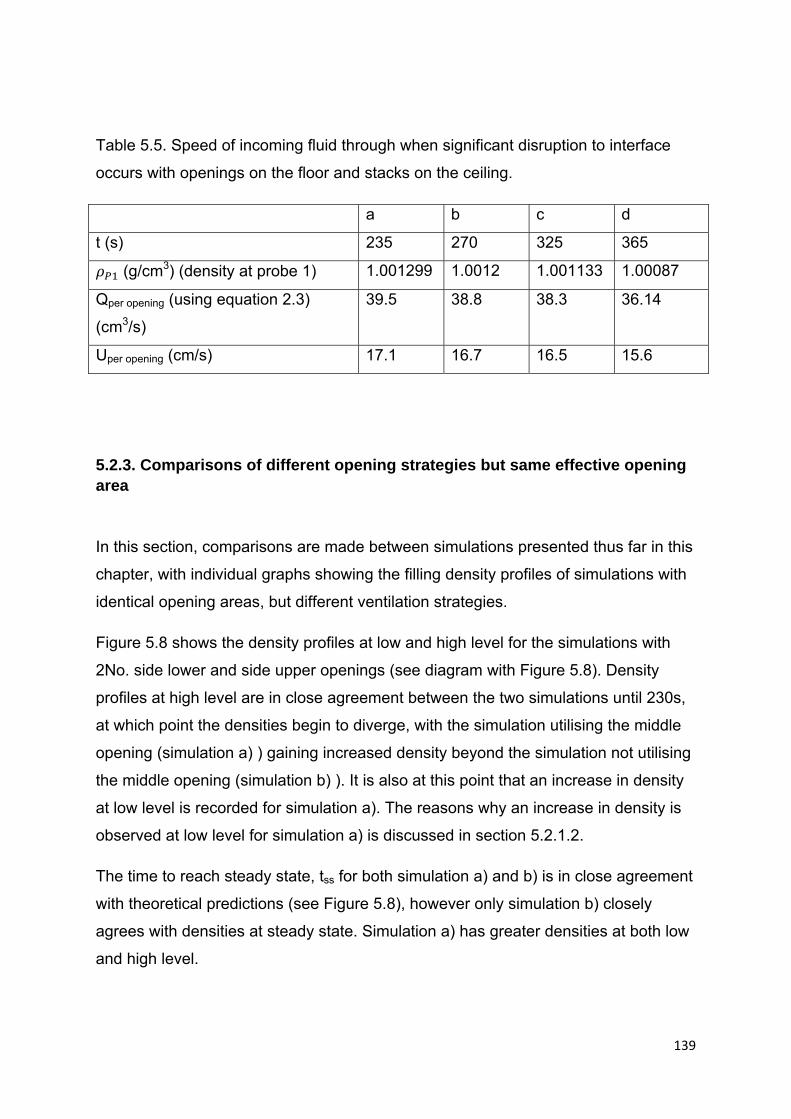
139
Table 5.5. Speed of incoming fluid through when significant disruption to interface
occurs with openings on the floor and stacks on the ceiling.
a b c d
t (s) 235 270 325 365
(g/cm3) (density at probe 1) 1.001299 1.0012 1.001133 1.00087
Qper opening (using equation 2.3)
(cm3/s)
39.5 38.8 38.3 36.14
Uper opening (cm/s) 17.1 16.7 16.5 15.6
5.2.3. Comparisons of different opening strategies but same effective opening area
In this section, comparisons are made between simulations presented thus far in this
chapter, with individual graphs showing the filling density profiles of simulations with
identical opening areas, but different ventilation strategies.
Figure 5.8 shows the density profiles at low and high level for the simulations with
2No. side lower and side upper openings (see diagram with Figure 5.8). Density
profiles at high level are in close agreement between the two simulations until 230s,
at which point the densities begin to diverge, with the simulation utilising the middle
opening (simulation a) ) gaining increased density beyond the simulation not utilising
the middle opening (simulation b) ). It is also at this point that an increase in density
at low level is recorded for simulation a). The reasons why an increase in density is
observed at low level for simulation a) is discussed in section 5.2.1.2.
The time to reach steady state, tss for both simulation a) and b) is in close agreement
with theoretical predictions (see Figure 5.8), however only simulation b) closely
agrees with densities at steady state. Simulation a) has greater densities at both low
and high level.

140
Because of the warmer internal environment, the mixing strategy might be more
appropriate during winter, as incoming fresh air is pre warmed reducing droughts.
This may also reduce heating requirements for the space.
Figure 5.8.Filling simulations with openings on the walls which have 2No. openings
at low and high level, where density profiles are at high level and low level.
Figure 5.9 shows the density profiles at low and high level for the simulations with
4No. side lower and side upper openings (see Figure 5.9). Density profiles at high
level are in close agreement between the two simulations until 400s, at which point
the densities begin to diverge, with the simulation utilising the middle opening
(simulation a) ) gaining increased density beyond the simulation not utilising the
middle opening (simulation b) ). Both simulation a) and b) closely agree with
theoretical time to reach steady state predictions, however only simulation b) shows
close agreement with theoretical steady state densities.
The divergence at high level between simulations a) and b) is smaller between the
simulations with 4No. openings than 2No. openings. This is due to increased dilution
by the non-middle openings in simulation a).
Simulation
Norm
alised
converted den
sity

141
0
0.5
1
1.5
2
2.5
3
0 200 400 600 800 1000 1200 1400
Norm
alised converted density
Time (s)
4[SI(2)&MI(2):4[SO(2)&MO(2)] P1
4[SI(2)&MI(2):4[SO(2)&MO(2)] P2
4SI:4SO P1
4SI:4SO P2
Theoretical density SS
Theoretical Tss
Theoretical density at steady state
Theoretical time to steady state
Figure 5.9.Filling simulations with openings on the walls which have 4No.openings at
low and high level, where density profiles are at high level and low level.
Figure 5.10, 5.11, 5.12 and 5.13 shows the density profiles at low and high level for
the simulations with openings located on the floor and ceiling, with stack and non-
stack simulations with the same openable area compared in each figure.
Simulation
a)
b)

142
0
1
2
3
4
5
6
7
0 500 1000 1500 2000 2500
Norm
alised converted density
Time (s)
1TI:1BO (S) P1
1TI:1BO( S) P2
1TI:1BO P2
1TI:1BO P1
Figure
5.10.Filling simulations with openings on the floor and ceiling which have
1No.openings at low and high level, where density profiles are at high level and low
level.
Figure 5.11.Filling simulations with openings on the floor and ceiling which have
2No.openings at low and high level, where density profiles are at high level and low
level.
a)
b)
a)
Simulation
0
0.5
1
1.5
2
2.5
3
3.5
4
4.5
0 200 400 600 800 1000 1200 1400 1600 1800
Norm
alised converted density (kg/m
3x1
0‐5)
Time (s)
2TI:2BO(S) P2
2TI:2BO(S) P1
2TI:2BOP2
2TI:2BOP1
a)
b)
Simulation
Norm
alised
converted den
sity

143
Figure 5.12.Filling simulations with openings on the floor and ceiling which have
3No.openings at low and high level, where density profiles are at high level and low
level.
Figure 5.13.Filling simulations with openings on the floor and ceiling which have
4No.openings at low and high level, where density profiles are at high level and low
level.
0
0.5
1
1.5
2
2.5
3
3.5
0 200 400 600 800 1000 1200
Norm
alised converted density
Time (s)
Series1
Series2
Series3
Series4
0
0.5
1
1.5
2
2.5
0 200 400 600 800 1000 1200
Norm
alised converted density
Time (s)
4TI:4BO (S) P1
4TI:4BO (S) P2
4TI:4BO P1
4TI:4BO P2
a)
b)
a)
b)
Simulation
Simulation

144
Stacks are often used in natural ventilation strategies to increase the flow through
the space, F, theoretically resulting in a higher interface and lower internal
temperatures. Table 5.6 details the steady state densities at low and high level
shown in Figures 5.10-5.13. For the simulations with 1No.opening at low and high
level, steady state densities at both low and high level are greater for the scenario
without stacks. This suggests that temperatures at both low and high level are cooler
as a result of the installation of the stack, which is in agreement with the theory
discussed in Chapter 2.
However, this is not observed when the number of openings is increased at both low
and high level to 2No. openings. This results in densities at low and high level
matching between non stack and stack simulations when steady state is reached.
Further increasing the number of openings at low and high level to 3No.and
4No.results in the density at low level being greater for the scenarios with the stacks,
however the density at high level is greater for the scenario without the stacks. The
increased flow due to stacks results in significant disturbance of the interface such
that the density at low level increases beyond that of the non-stack scenario. Results
from section 5.2.1.2 showed that when a mixed layer at low level forms, the plume
will lose less buoyancy compared with a scenario without the mixed layer resulting in
a layer at high level with increased buoyancy. This does not occur because F is
significantly greater due to stacks.

145
Table 5.6. Speed of incoming fluid through opening when significant disruption to
interface occurs with openings on the floor and ceiling.
Comparisons between theoretical and experimental values for time to reach steady
state and density are made in Table 5.7 for the simulations detailed up to this point
within this section. Chenvidyakarn and Woods (2005) used equation 5.1 to calculate
tts, which is a timescale to converge to steady state and this was used to compare
theoretical and experimental values within table 5.7.
∗ 5.1
where V is the volume of the model including any stacks, tss is the temperature at
steady state and Ta is the ambient temperature. The use of this equation requires a
conversion between temperature and density to be useful for water bath simulations.
Care is required when using equation 5.1 as it is very sensitive to changes in .
Chenvidyakarn and Woods (2005) used a value of 0.0003.
Theory predicts that time to reach steady state is greater for simulations with stacks
than the simulations without. This is due to the theory calculating a larger difference
in density within the model between stack and non-stack scenarios of the same
opening area than what experimentally occurs. The reason why experimental
densities are significantly greater than theoretical values is due to the mixed layer
leading to reduced dilution of the plume. This in turn leads to shorter Tss values.
No. Lower
openings
No. Upper
openings
Stack? Density at
low (kg/m3)
Density at
high (kg/m3)
1 1 No 1.002 1.005
1 1 Yes 1.0015 1.004
2 2 No 1.0004 1.0027
2 2 Yes 1.0004 1.0027
3 3 No 0.9997 1.0021
3 3 Yes 0.9999 1.0018
4 4 No 0.9994 1.0013
4 4 Yes 0.9996 1.0011

146
There is no correlation between the theory and experimental results, which suggests
that the theory does not describe scenarios with a non-traditional flow regime.
Table 5.7.Experimental and theoretical data for density and time to reach steady
state for simulations with openings on the bottom and top of model.
Experimental values Theoretical
Density at P2
(g/cm3)
tss(s) Density below interface
(g/cm3)
tss (s)
1BI:1TO 1.005 2000 1.00337 3006
1BI:1TO (S) 1.004 1300 1.00235 3404
2BI:2TO 1.0028 1350 1.001961 1759
2BI:2TO (S) 1.0028 1050 1.001238 1949
3BI:3TO 1.0021 900 1.00144 1384
3BI:3TO (S) 1.0019 900 1.000813 1444
4BI:4TO 1.0013 900 1.00109 1181
4BI:4TO (S) 1.0011 900 1.000518 1223
Two final comparisons are produced in this section:
- all simulations with 2No. openings at low and high level
- all simulations with 4No. openings at low and high level.
Figure 5.14 shows the filling densities for all 2No. opening at low and high level
simulations so far mentioned in this chapter. Simulation a) has openings on the floor
and stacks on the ceiling, b) has openings on the floor and ceiling, c) uses openings
at low and high level on the side positioned such to disturb the plume and d) has low
and high level openings on the side which will not disturb the plume.
Between all four simulations, the only variable is the location of the openings.
According to the theory described in chapter 2, simulation a) should have the highest
interface and lowest internal density due to its significantly larger H. Simulations c)
and d) should have the lowest interface and highest internal density due to their
reduced H. However, the experiments show that simulation c) has the greatest
density and simulation d) has the lowest density at high level. The mixing regimes
147
that occur in simulations a) and b) cause internal densities to increase beyond what
the theory predicts, negating the effect of increased H.
At low level, the densities are greatest for simulations a) and b) with no increase in
density measured for simulation d).

148
0
0.5
1
1.5
2
2.5
3
3.5
4
4.5
0 500 1000 1500 2000
Norm
alised converted density
Time (s)
2BI:2TO (S)
2BI:2TO
2MI:2MO
2SI:2SO
0
0.2
0.4
0.6
0.8
1
1.2
1.4
1.6
1.8
0 500 1000 1500 2000
Norm
alised converted density (g/cm
3x1
0‐4)
Time (s)
2BI:2TO (S)
2BI:2TO
2MI:2MO
2SI:2SO
i)
ii)
Figure 5.14.Filling simulations with openings on the side or on the floor and ceiling
which have 2No. openings at low and high level, where density profiles are at high
level, i) and low level, ii).
a)
b)
c)
d)
a)
b)
c)
d)
Simulation
Simulation
149
Figure 5.15 shows the filling densities for all 4No. opening at low and high level
simulations so far mentioned in this chapter. Simulation a) has openings on the side
wall such to ensure incoming fresh water collides with the plume, b), has openings
on the floor and ceiling of the model, c) has openings on the floor and stacks on the
ceiling and d) has openings on the side wall placed such to ensure no collision with
the plume.
The theory would predict that simulation a) and d) will achieve the highest internal
densities due to their lower H, with simulation c) achieving the lowest internal
densities due to greatest H. At high level, a) achieves the highest density (1.00135
g/cm3) however this is largely due to the mixing that takes places rather than smaller
H (see section 4.4.1.2) which is closely followed by simulation b) (1.0013 g/cm3).
Simulation c) achieves the lowest density at high level.
At low level, simulation c) achieves the greatest internal density, followed by
simulation a and then b). Simulation d) records no change in density. Importantly, for
the 2No.opening simulations discussed earlier in this section, densities at low level
for simulation c) is the same for the 4No. opening simulation c). This suggests whilst
increasing opening area will reduce internal densities, a different ventilation strategy
with a smaller opening area can achieve the same results.
Whilst simulation c) will theoretically have the greatest F through the space, internal
densities at low level are also greatest. This suggests that simulation c) and to a
lesser degree, simulation a) and b) will be appropriate during winter months, causing
a warming of the environment at low level. However, during the summer months,
these strategies would not be appropriate for a naturally ventilated strategy as they
would likely result in increased overheating for the occupants. Simulation d) is more
appropriate for summer months.

150
0
0.1
0.2
0.3
0.4
0.5
0.6
0.7
0.8
0.9
1
0 200 400 600 800 1000 1200 1400
Norm
alised converted density
Time (s)
0
0.5
1
1.5
2
2.5
3
0 200 400 600 800 1000 1200 1400
Norm
alised converted density
Time (s)
1
2
3
4
Figure 5.15.Filling simulations with openings on the side or on the floor and ceiling
which have 4No. openings at low and high level, where density profiles are at high
level, i) and low level, ii).
c)
d)
a)
Simulation
Simulation
i)
ii)
151
5.5 Draining comparisons of note
Section 5.4 showed the density profiles for simulations with different opening areas
and ventilation strategies until steady state was reached. After steady state was
reached, the flow of brine into the model was turned off and this section reports of
the density profiles of draining until ambient densities are reached at P1 and P2.
Understanding how effective a ventilation strategy is at ensuring a thermally
comfortable environment is imperative to reduce the requirements for air conditioning,
heating and flushing pollutants. However it is also important to select a ventilation
strategy which ensures that the space is purged quickly of warmer than ambient air
and pollutants when not in use, so that it is ready to be used again.
This section aims to show which opening strategies provide the best capability for
purging. It was shown in section 4.3 that the draining of the model closely follows
theoretical predictions and the observations of other researchers, which provides
confidence that the more complicated draining scenarios shown in this section will
also simulate real life conditions. Firstly, simulations using the same ventilation
strategy and towards the end of this section, simulations using different ventilation
strategies, but identical opening areas are compared.
Figure 5.16 compares the density draining profiles for all opening strategies which
have 2No. openings at low and high level. Simulation a) has openings on the floor
and ceiling, simulation b) has openings on the floor and stacks on the ceiling,
simulation c) has openings on the side placed such to ensure traditional
displacement ventilation and d) openings on the side placed such to ensure mixing.

152
i)
ii)
Figure 5.16.Emptying simulations with openings on the side or on the floor and
ceiling which have 2No.openings at low and high level, where density profiles are at
high level, i) and low level, ii).
Simulation
Simulation
Norm
alised
converted den
sity
Norm
alised
converted den
sity

153
At high level, the densities at t = 0s for the four simulations are all within 0.0004g/cm3,
however, the time to drain is quite varied. Simulation c) is completely drained by
1500s, with a) and b) draining by 2400s and simulation d) draining by 3500s. The
difference in draining time between all four simulations is due to the different
ventilation regimes that occur.
At the beginning of each draining density profile, densities are reasonably stable and
do not fluctuate. This means that the fluid at high level is homogenous and assuming
that the interface was not disrupted, this homogenous layer will extend from the
ceiling down to the interface. After the layer above the interface has drained, the
measured density begins to reduce, but remains above ambient for over 50% of the
total time of draining. For simulation c), the mixed layer is approximately 1cm deep
which is considerably smaller than the depth of the layer above the interface but
takes longer to drain. This is because the mixed layer has a lower density, resulting
in reduced buoyancy forces. However, for the other scenarios, draining takes
considerably longer due to the mixed layer being considerably larger (Simulations b),
c) and d)) and/or ventilation regime continues to cause mixing within the internal
space ((simulations a) and b)).
The density profile for the simulation b) which has the stack shows a considerably
smaller homogenous layer above the interface compared with the simulations
without stacks. This can be explained by Figure 5.17 which shows how the
penetration of incoming fluid is sufficiently significant that it manages to penetrate
through most of the model. This results in a shallow homogenous layer at the top of
the model, with a non-homogenous layer below the interface which increases in
buoyancy with height. Because the stacks encourages more flow through the
openings, there is a greater penetration with the stack scenario.
The penetration of incoming fluid decreases with time due to reduced F throughout
the model. It is the penetration of fluid which causes mixing below the interface
resulting in draining where an interface does not form. This leads to a considerably
longer period for draining to be completed at low level in the building compared with
opening strategies which use side inlets. Stacks exacerbate this mixing which results
in the stack strategy taking considerably longer to drain.

154
Figure 5.17.Penetration of incoming ambient fluid through a draining simulation with
openings on the top and bottom of the model.
Figure 5.18 compares the density draining profiles for all opening strategies which
have 4No. openings at low and high level. Simulation a) has lower and upper
openings on the side placed such to avoid disruption of the plume, b) has openings
on the floor and ceiling, c) has openings on the floor and stacks on the ceiling and d)
has lower and upper openings on the side placed such to ensure disruption of the
plume.
The simulations with 4No.openings at low and high level follow the trends noted for
the 2No. opening simulations noted earlier in this section. The simulations which
followed a mixing strategy rather than traditional displacement took longer to drain.
The extent at which mixed regions increase draining time becomes clear when
comparing the 2No. opening simulation c) and the 4No. opening simulations which
used mixing strategies. The 2No.opening simulation drains by 1500s whilst the 4No.
opening simulations drains by 1800s.

155
In conclusion, whilst increasing opening areas does decrease draining time,
depending on the draining strategy and initial thermal environment, a smaller
opening area could achieve faster draining times if a different draining strategy was
used. In particular, stacks which are usually applied to naturally ventilated strategies
to increase F and therefore reduce draining times may not be as effective compared
with openings at low and high level on the walls.
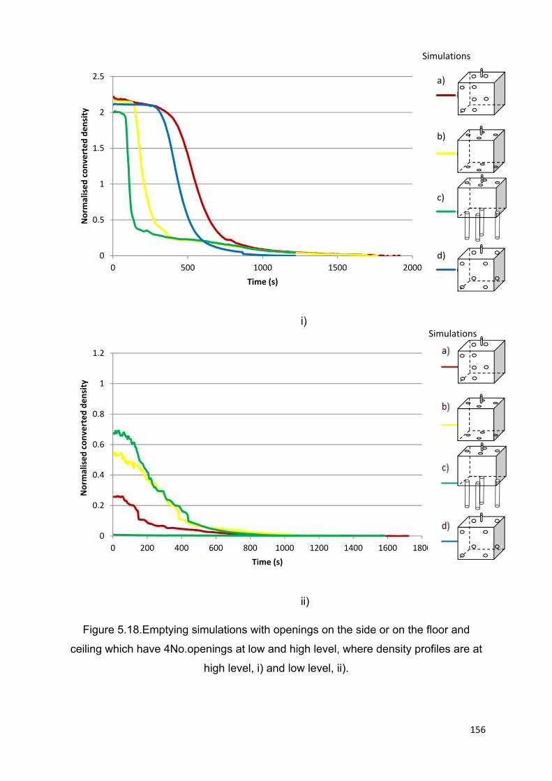
156
i)
ii)
Figure 5.18.Emptying simulations with openings on the side or on the floor and
ceiling which have 4No.openings at low and high level, where density profiles are at
high level, i) and low level, ii).
0
0.5
1
1.5
2
2.5
0 500 1000 1500 2000
Norm
alised converted density
Time (s)
b
c
d
e
0
0.2
0.4
0.6
0.8
1
1.2
0 200 400 600 800 1000 1200 1400 1600 1800
Norm
alised converted density
Time (s)
d)
b)
c)
a)
Simulations
Simulations

157
5.6 Summary
This chapter has compared water bath model experiments with natural ventilation
theory for a simple cube shaped room with openings positioned on its side, floor,
ceiling and stacks. It was shown that for cases where the brine plume is not
disturbed by incoming fluid and where a mixed layer below the interface remains
small in magnitude, interface heights, time to empty, time to reach steady state, and
densities above the interface all closely agree with the theory. However, when the
interface is disturbed, experimental results differ from theoretical predictions.
Natural ventilation within a simple room was simulated in the water bath using
several opening strategies. The four types of ventilation strategies assessed in this
chapter have openings located as follows:
Strategy 1: Floor and ceiling
Strategy 2: Floor and stacks on the roof
Strategy 3: Low and high level openings on the wall (not inline with the plume)
Strategy 4: Low and high level openings on the wall (inline with the plume)
Density profiles for each of these strategies were compared, allowing for densities,
time to reach steady state and time to drain to be investigated to determine the
effectiveness of each strategy. The theory presented in chapter 2 states that as H
increases, F will increase resulting in reduced internal temperatures. As a result, the
theory predicts that when all parameters are identical except opening location,
strategy 2 will have the lowest internal densities, followed by 1 with 3 and 4 having
identical internal densities.
Simulations presented in this chapter showed that the increase in F for strategy 1
and 2 causes significant penetration and disruption of the interface, resulting in
increased densities at low level. Strategy 4 achieves densities at low level which was
approximately halfway between ambient densities and those recorded by strategy 1
and 2. No increase in density beyond ambient was measured in strategy 3. If this
also occurs within a naturally ventilated building, it suggests that the stack ventilation
strategy is detrimental to a building designer's aim to reduce internal temperatures.

158
However, during winter, strategies 1, 2 and 4 could be preferable as it would reduce
heating requirements whilst also limiting droughts which can cause thermal
discomfort.
It was also found that whilst increasing the opening area for a strategy will reduce
the internal densities, a different strategy with a reduced opening area could achieve
similar internal densities. This is an important consideration because naturally
ventilated buildings usually require large openable areas to achieve a thermally
comfortable environment, which is not always easily achieved. For example, strategy
4 achieves the same densities at low level as strategy 1 and 2 but with half the
openable area at both low and high level.
Purging a space of warmer-than-ambient air is an important strategy to reduce
overheating, especially during summer which will often include night purging. The
speed at which the strategies drain was investigated as a result of this importance.
When comparing identical opening areas, strategy 3 was always the fastest to drain,
with strategies 1 and 2 draining at the equally slowest times. Slower purging
occurred due to mixed layers of density less than the homogenous layer above the
interface and also the continued mixing of the internal space during draining. For
example, strategy 3 with half the openable area at both low and high level of strategy
1 and 2 drains 300s faster.
The work in this chapter highlights the limitations of current theoretical equations,
with particular reference to mixed layers and disrupted interfaces resulting in
significantly different temperatures and draining times. Both mixed layers and
disrupted interfaces causes strategies 1, 2 and 4 to perform considerably worse than
what the theory predicts. The results obtained from simulations of strategy 3 were
found to be in close agreement with the theory and the findings of other researchers
due to the mixed layer being insignificant in depth and there being no disrupted
interfaces.
Perhaps most importantly, this chapter has shown that different opening strategies
can be implemented to achieve specific internal thermal environments. For example,
the use of openings low level openings with stacks causes significant disruption to
the stratified layer of warm air at high level, resulting in warm air at high level being
forced downwards. Such a strategy could be effective when heating is required.

159
Importantly, much of the work in the latter part of this chapter shows little agreement
with current theory and this is due to mixed layers and the interface and plumes
becoming disrupted by incoming fluid.

160
Chapter 6. Benchmark 2 (Open plan office)
6.1. Preamble.
Time dependant flows can cause permanent changes to the flow regime of a natural
ventilation strategy, resulting in increases or decreases in internal temperatures and
flow rates. Such changes could be detrimental or favourable depending on internal
and external temperatures. This chapter assesses the possibility of controlling
different flow regimes within a space to influence internal temperatures with the aim
to ensure a thermally comfortable naturally ventilated space.
6.2. Introduction
For a naturally ventilated room, if wind with strength less than the NV driving forces
blows towards the upper opening, then the volume of air flowing through the upper
opening will reduce compared with the scenario where there is no wind (Figure 6.1a
and b). This will result in a lower interface height, which may cause thermal
discomfort to occupants whilst also exposing them to stale air. If the force of wind is
greater than the NV driving forces, then the NV flow regime is changed, with ambient
air flowing through the upper opening, forcing internal air to flow through the lower
opening (Figure 6.1c). If such an event occurred during winter, it is likely that the
heater placed at the lower opening will continuously heat air which is flowing out of
the room, resulting in significant heating costs whilst the room remains cold and
likely uncomfortable for any occupants. Such flow regime changes can be
permanent, even if the wind was temporary and in such situations, are termed 'time
dependant flows'.

161
.
a) b) c)
Figure 6.1. A naturally ventilated space where a), the driving forces are undisturbed
by external forces, b) driving forces are reduced in strength by a weak wind and c)
where driving forces are overpowered and the flow regime is fundamentally changed.
The size of an arrow represents the quantity of air flowing through an opening.
Work was undertaken by Chenvidyakarn and Woods (2004) to better understand the
principles of wind overpowering the driving forces of naturally ventilated air flow,
forcing the direction of flow to permanently change. It was shown that for a model
with an opening at low level and two stacks at high level, it was possible for three
flow regimes to occur (Figure 6.2), each causing different internal temperatures.
Flow regime A and C involved only one of the two stacks behaving as an outlet
whilst flow regime B involved both stacks acting as outlets. The effective opening
area of an opening, ∗ , is calculated by multiplying the opening area by the
coefficient of discharge, Cd, which was taken as 0.61 within this work.
wind wind
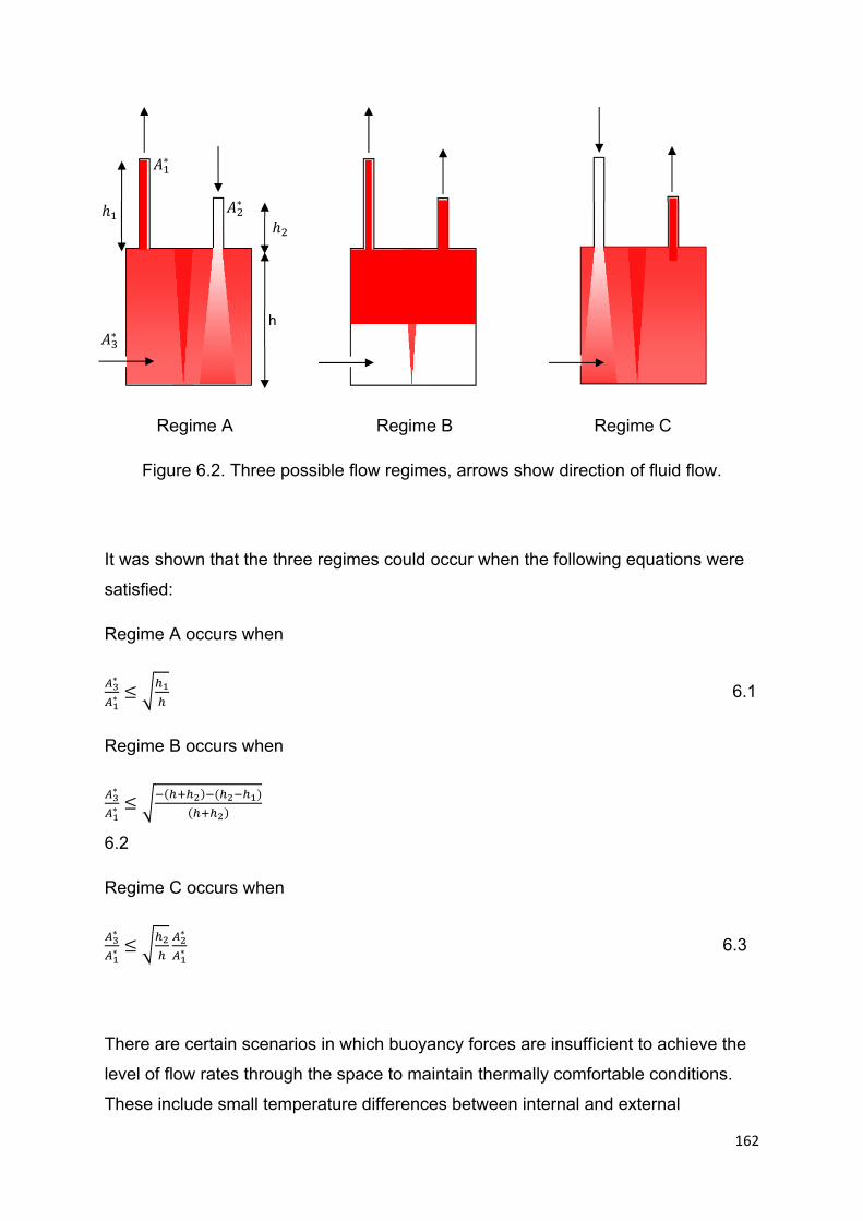
162
Regime A Regime B Regime C
Figure 6.2. Three possible flow regimes, arrows show direction of fluid flow.
It was shown that the three regimes could occur when the following equations were
satisfied:
Regime A occurs when
∗
∗ 6.1
Regime B occurs when
∗
∗
6.2
Regime C occurs when
∗
∗
∗
∗ 6.3
There are certain scenarios in which buoyancy forces are insufficient to achieve the
level of flow rates through the space to maintain thermally comfortable conditions.
These include small temperature differences between internal and external
h ∗
∗
∗

163
temperatures or inadequate opening areas. These problems can be overcome by
taking advantage of different flow regimes which can cause different internal
temperatures. Whilst the forces of wind can cause unpredictable and potentially
undesirable changes in flow regimes within a naturally ventilated space, this chapter
assesses the plausibility of intentionally forcing regime change within a naturally
ventilated space with the intention to improve the thermal environment of the space.
6.3 Methodology
The simulations conducted within this chapter were undertaken within a 29cm cube
box with 1No. 1.6cm diameter opening at low level and 2No.stacks with 1.9cm
internal diameters extending beyond the ceiling (Figure 6.3). The brine source is
located within the centre of the floor of the model using the nozzle described in
chapter 3.4.6. and simulates a 50W heat source, which was calculated using the
scaling equations described in section 3.3.1. The lower level opening was
strategically placed to ensure incoming ambient fluid did not collide with the plume.
Probe located at low level
within the model
Probe located at high level
within the model
Figure 6.3. Diagram of model used to produce 'mechanically induced' time
dependant flows.
Regimes A, B and C occur when their respective equations (5.1, 5.2 and 5.3) are
found to be true. Table 6.1 shows when each of the three flow regimes can occur if
29cm
29cm 20cm
Floor
Ceiling

164
the height of the short stack, is 20cm, height of the tall stack, is 29cm and the
floor to ceiling height, h is 29cm. These heights remained the same for all
simulations conducted within this chapter. If a cell is highlighted in green, then the
flow regime can occur for that specific lower opening area, whilst red states that the
flow regime can not occur. Conductivities were measured at both low and high level,
with measurements automatically recorded every 5 seconds.
Table 6.1.Predictions for flow regime A, B and C to occur with varying effective lower
opening area.
Flow regime A Flow regime B Flow regime C
∗ ∗
∗ <
∗
∗ ∗
∗ ∗
∗
0.019 0.01 < 1 0.01 0.43 0.01 0.83
0.076 0.04 < 1 0.04 0.43 0.04 0.83
0.17 0.09 < 1 0.09 0.43 0.09 0.83
0.30 0.16 < 1 0.16 0.43 0.16 0.83
0.48 0.25 < 1 0.25 0.43 0.25 0.83
0.69 0.36 < 1 0.36 0.43 0.36 0.83
0.94 0.49 < 1 0.49 0.43 0.49 0.83
1.22 0.64 < 1 0.64 0.43 0.64 0.83
1.55 0.81 < 1 0.81 0.43 0.81 0.83
1.91 1 < 1 1 0.43 1 0.83
Fan assisted natural ventilation is a strategy which is increasingly being used to
ensure adequate flow rates when the buoyancy effect is insufficient to provide free
cooling (Breathing Buildings 2014). This could occur when internal and external
temperatures are similar (e.g. in the summer) or when there is an unusually high
heat gain within the space and the openings are insufficiently sized. Whilst
Chenvidyakarn and Woods (2004) assumed that wind would cause the change in
flow regime, it is entirely possible that fans located within the stacks can
automatically activate for a short period of time to force the flow regime within the

165
space to change. This would allow for a controlled approach which would negate the
unpredictability of wind.
In the water bath model, fans were simulated within each of the stacks by injecting or
extracting fluid from one of the stacks using an adjustable volume pipette which was
capable of injecting or extracting up to 20ml. Extracting fluid simulated a fan
expelling air from the space into the environment, whilst injecting fluid simulated a
fan supplying ambient air into the space. An adjustable volume pipette was used to
ensure accurate control of the volume of fluid injected or extracted into/from the
stacks.
Initial simulations were conducted with varying the lower opening radius between 0.2,
0.4 0.8 and 1cm. When steady state was reached, one of the three flow regimes was
observed (Table 6.2) and attempts to force the flow regime to change were made.
Switching flow regimes between A and B required the supply or extraction of 5ml of
fluid, B and C the supply or extraction of 20ml and C to A, the supply or extraction of
10ml of fluid (Figure 6.4). For scenarios where the flow regime would not change,
due to lower opening area to another flow regime (refer to Table 6.1), large
quantities (up to 200ml) of fluid were injected or extracted from a stack in an attempt
to force the regime to change, however this was never successful.
Table 6.2. Experimental regimes observed with varying lower opening area.
∗ Initial regime New regimes Theoretical agreement
0.076 A C Yes
0.30 A C Yes
1.22 A C and A Yes
1.91 B A Yes
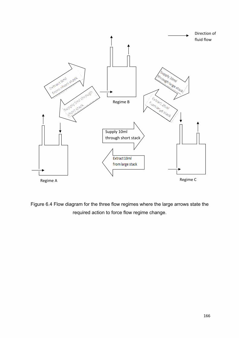
166
Supply 10ml
through short stack
Figure 6.4 Flow diagram for the three flow regimes where the large arrows state the
required action to force flow regime change.
Direction of
fluid flow
Regime A
Regime B
Regime C
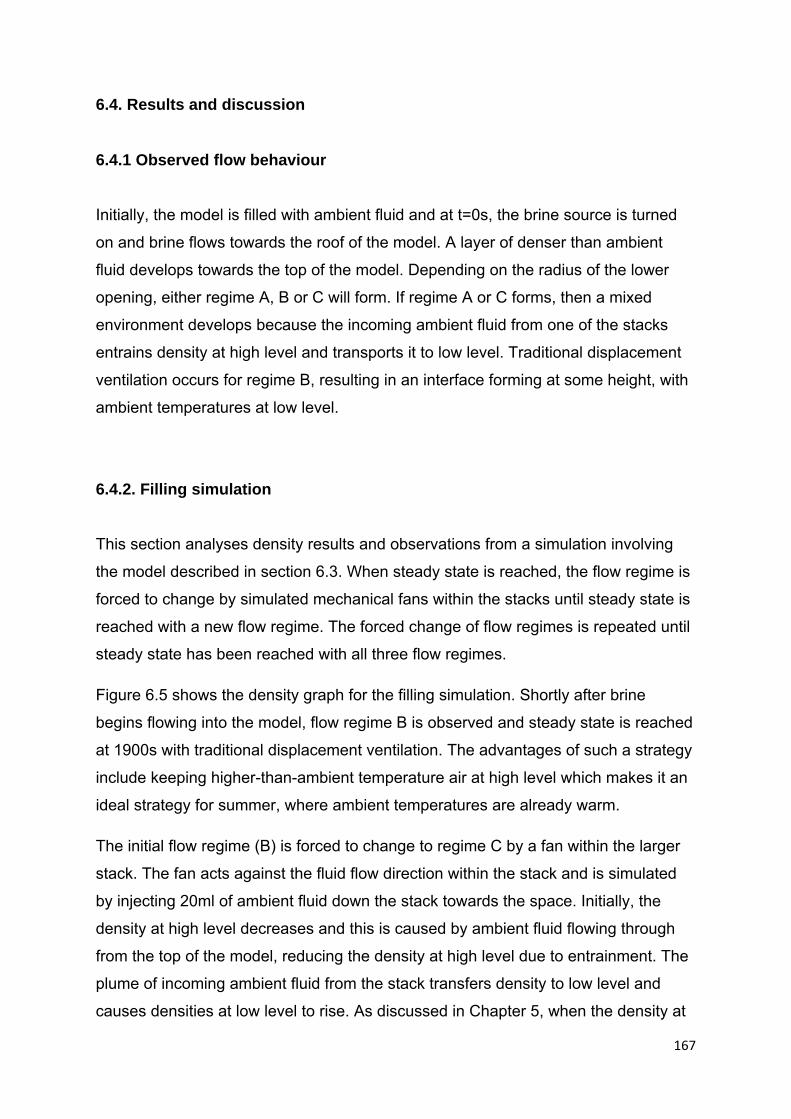
167
6.4. Results and discussion
6.4.1 Observed flow behaviour
Initially, the model is filled with ambient fluid and at t=0s, the brine source is turned
on and brine flows towards the roof of the model. A layer of denser than ambient
fluid develops towards the top of the model. Depending on the radius of the lower
opening, either regime A, B or C will form. If regime A or C forms, then a mixed
environment develops because the incoming ambient fluid from one of the stacks
entrains density at high level and transports it to low level. Traditional displacement
ventilation occurs for regime B, resulting in an interface forming at some height, with
ambient temperatures at low level.
6.4.2. Filling simulation
This section analyses density results and observations from a simulation involving
the model described in section 6.3. When steady state is reached, the flow regime is
forced to change by simulated mechanical fans within the stacks until steady state is
reached with a new flow regime. The forced change of flow regimes is repeated until
steady state has been reached with all three flow regimes.
Figure 6.5 shows the density graph for the filling simulation. Shortly after brine
begins flowing into the model, flow regime B is observed and steady state is reached
at 1900s with traditional displacement ventilation. The advantages of such a strategy
include keeping higher-than-ambient temperature air at high level which makes it an
ideal strategy for summer, where ambient temperatures are already warm.
The initial flow regime (B) is forced to change to regime C by a fan within the larger
stack. The fan acts against the fluid flow direction within the stack and is simulated
by injecting 20ml of ambient fluid down the stack towards the space. Initially, the
density at high level decreases and this is caused by ambient fluid flowing through
from the top of the model, reducing the density at high level due to entrainment. The
plume of incoming ambient fluid from the stack transfers density to low level and
causes densities at low level to rise. As discussed in Chapter 5, when the density at
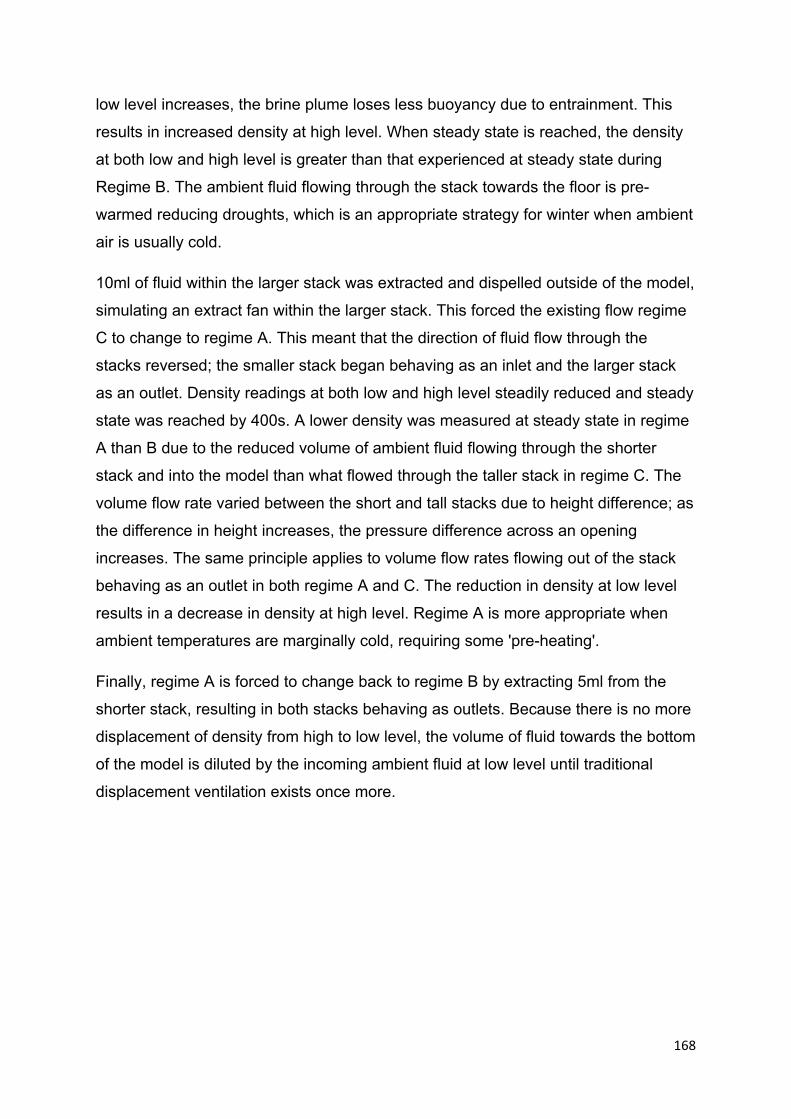
168
low level increases, the brine plume loses less buoyancy due to entrainment. This
results in increased density at high level. When steady state is reached, the density
at both low and high level is greater than that experienced at steady state during
Regime B. The ambient fluid flowing through the stack towards the floor is pre-
warmed reducing droughts, which is an appropriate strategy for winter when ambient
air is usually cold.
10ml of fluid within the larger stack was extracted and dispelled outside of the model,
simulating an extract fan within the larger stack. This forced the existing flow regime
C to change to regime A. This meant that the direction of fluid flow through the
stacks reversed; the smaller stack began behaving as an inlet and the larger stack
as an outlet. Density readings at both low and high level steadily reduced and steady
state was reached by 400s. A lower density was measured at steady state in regime
A than B due to the reduced volume of ambient fluid flowing through the shorter
stack and into the model than what flowed through the taller stack in regime C. The
volume flow rate varied between the short and tall stacks due to height difference; as
the difference in height increases, the pressure difference across an opening
increases. The same principle applies to volume flow rates flowing out of the stack
behaving as an outlet in both regime A and C. The reduction in density at low level
results in a decrease in density at high level. Regime A is more appropriate when
ambient temperatures are marginally cold, requiring some 'pre-heating'.
Finally, regime A is forced to change back to regime B by extracting 5ml from the
shorter stack, resulting in both stacks behaving as outlets. Because there is no more
displacement of density from high to low level, the volume of fluid towards the bottom
of the model is diluted by the incoming ambient fluid at low level until traditional
displacement ventilation exists once more.
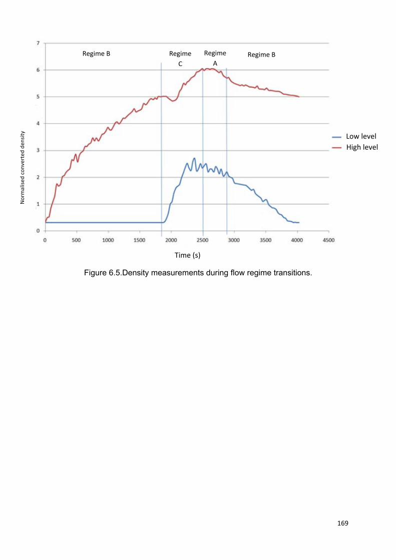
169
Figure 6.5.Density measurements during flow regime transitions.
Regime B Regime
C
Regime
ARegime B
Time (s)
Low level
High level
Norm
alised converted den
sity
170
6.4.3 Draining simulations
After steady state is reached for the simulation discussed in section 6.4.2, with the
active flow regime being regime B, the brine source is turned off and the model is
allowed to empty. Densities at low and high level are measured and the density
profiles are shown in Figure 6.6.
At t=0s, the brine source is turned off and draining begins with Regime B. The
density at high level remains constant for the first 480 seconds and density at low
level remains at ambient levels, which shows that traditional displacement ventilation
occurred as discussed in chapter 4. However, at 480 seconds, the flow regime
switches to flow regime C and the taller stack begins to behave as an inlet.
The natural switching in flow regime has a consequential effect on draining and
results in the denser-than-ambient layer above the interface being diluted by the
incoming ambient fluid. This causes draining to take considerably longer than if
draining occurred with traditional displacement ventilation (see section 5.3.2.3). Fans
could be employed to ensure that the natural switching does not occur, but this may
require the fans to be active throughout the draining process, resulting in significant
energy requirements.
Due to the significant effect on time that the natural switching of flow regimes could
have whilst draining, further simulations were conducted with other lower opening
areas. It was found that the flow regime would change only when the lower opening
area was such that it was possible for all three flow regimes to occur. For example,
when ∗ = 1.91cm2, regime B naturally occurs when steady state is reached and the
model also drains with regime B. Because this regime causes an interface to form, it
is a considerably more efficient draining strategy than A and C which cause a mixed
internal environment (see section 5.4.4). A lower opening effective area of 1.22 cm2
is required to ensure that all three flow regimes can occur, which is important to
ensure thermally comfortable internal temperatures. To ensure both an efficient
draining solution and a thermally comfortable internal environment, the lower
opening area should be controlled by an automated louvre. This louvre should be
sized to ensure draining naturally occurs with regime B, but automatically reduce in
size to ensure that all three flow regimes can occur when draining is not in operation.
171
Figure 6.6. Emptying simulation with densities at low and high level with flow regime
automatically changing.
6.5 Summary of Benchmark 2
Chenvidyakarn and Woods (2004) showed that by using water bath modelling with
heated wires to simulate a distributed heat source, it was possible for up to three
different flow regimes to occur which resulted in different internal temperatures.
Simulations reported in this chapter show that water bath modelling using a point
source of brine can produce the same three flow regimes, resulting in different
internal temperatures in agreement with Chenvidyakarn and Woods (2004).
A simulation was conducted with a lower opening radius of 0.8cm and all three flow
regimes were simulated, forcing a change between the flow regimes by simulating
fans which extracted from a stack or expelled ambient air into a stack. Regime C
was shown to have the greatest internal densities at both low and high level within
the model followed by regime A. Regime B followed traditional displacement
ventilation and resulted in the lowest densities at high level and ambient densities at
low level. As a result, regime B is most appropriate for use during summer, whilst
0
1
2
3
4
5
6
0 500 1000 1500 2000 2500
Norm
alised converted density
Time (s)
Low level
high level
Time (s)
Regime
B Regime C

172
regime C is most effective when ambient temperatures are very cold (for example
winter) and regime A during cool ambient conditions (for example spring/autumn).
A draining simulation was also conducted when regime B was the active flow regime.
It was shown that after 8 minutes of draining, the flow regime switched to flow regime
C which resulted in considerably slower draining times due to the layer above the
interface within the model becoming diluted by the incoming ambient fluid from the
stack. The diluting of the incoming layer of higher-than-ambient density was also
observed in flow regime A simulations, with flow regime B simulations draining faster
than flow regimes A and C. To prevent the natural switch in flow regimes,
mechanical fans would be required, although this may significantly increase energy
usage of the natural ventilation strategy.
To ensure three flow regimes could occur and the space naturally drained with flow
regime B, a mechanical louvre would have to be used on the low level opening. This
louvre would automatically adjust its openable area to ensure that the flow regime
which would produce the most thermally comfortable thermal environment whilst the
room is occupied is active. The mechanical louvre will increase in size to ensure
draining with regime B when unoccupied occurs, which is the most efficient flow
regime for draining. The use of a mechanical louvre is a lower energy strategy than
relying on mechanical fans to maintain draining with flow regime B.

173
Chapter 7. Benchmark 3 (Hospital)
7.1. Preamble.
Natural personalised ventilation (NPV) strategies attempt to deliver fresh air to the
location of occupants within a room. This chapter investigates a NPV strategy
proposed for use within hospital wards, in particular looking at the influence that heat
source location has on the internal thermal environment. Results from CFD
simulations and the analytical model described in section 3 are also compared with
those from water bath simulations to provide validation. CFD simulations were
carried out by Z. Adamu, see Todd et al. (2014).
7.2. Introduction
Traditionally, naturally ventilated (NV) buildings are designed in such a way to
provide sufficient fresh air to a room, with little or no thought to the location of the
occupants. As a result, whilst sufficient fresh air might be delivered to the room, the
occupants, due to their location, may not actually receive sufficient fresh air. Natural
Personalised Ventilation (NPV) is a strategy where the ventilation design attempts to
provide fresh air directly to the occupants within the space, instead of just to the
room.
Such a design was successfully demonstrated for hospitals by Adamu et al. (2011),
using dynamic modelling (zonal airflow) and steady state computational fluid
dynamics (CFD). Both of these numerical methods are widely used in research and
industry, ensuring conservation of mass, energy, momentum and chemical and
biological species (Chen, 2009; Li and Nielsen, 2011).Computer simulations, whilst a
very powerful tool, is subject to its assumptions, and to the equations which they use.
Similarly, WBM uses water to simulate air and it is entirely possible that water does
not behave in the exact way that air does due to differences in viscosity. As a result,
comparing results from different simulation techniques will validate their results if
there is close agreement, providing confidence that the naturally ventilated hospital
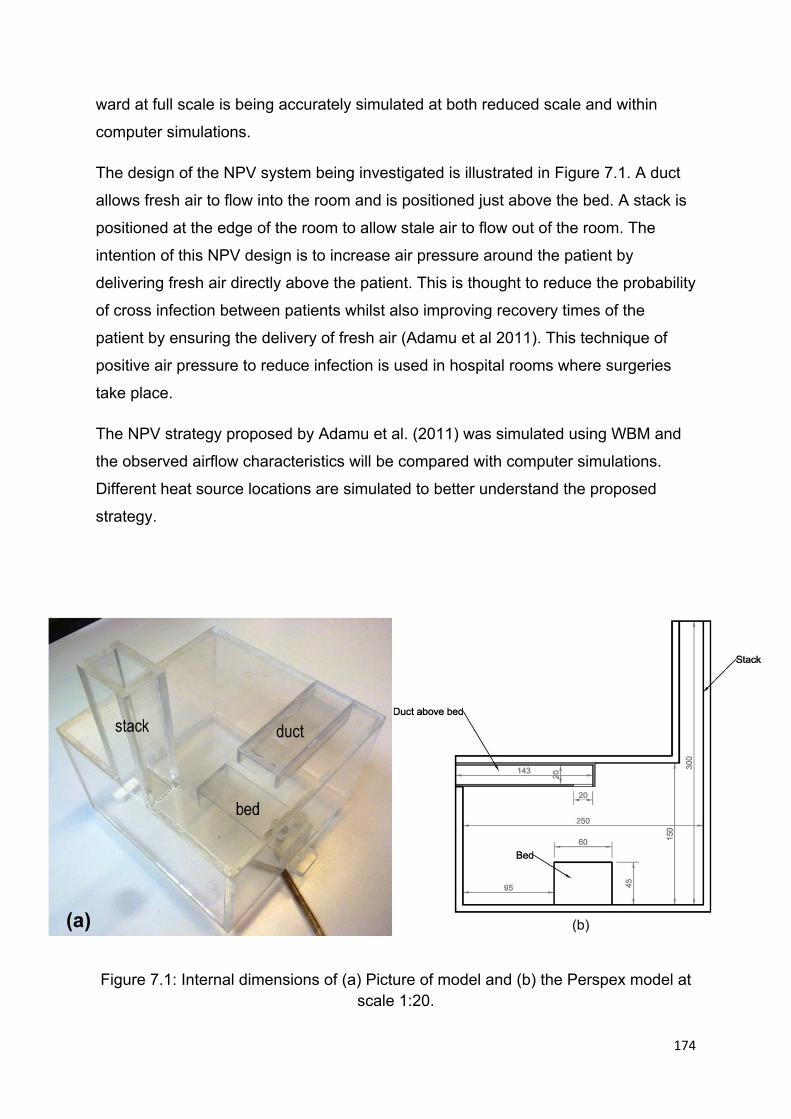
174
ward at full scale is being accurately simulated at both reduced scale and within
computer simulations.
The design of the NPV system being investigated is illustrated in Figure 7.1. A duct
allows fresh air to flow into the room and is positioned just above the bed. A stack is
positioned at the edge of the room to allow stale air to flow out of the room. The
intention of this NPV design is to increase air pressure around the patient by
delivering fresh air directly above the patient. This is thought to reduce the probability
of cross infection between patients whilst also improving recovery times of the
patient by ensuring the delivery of fresh air (Adamu et al 2011). This technique of
positive air pressure to reduce infection is used in hospital rooms where surgeries
take place.
The NPV strategy proposed by Adamu et al. (2011) was simulated using WBM and
the observed airflow characteristics will be compared with computer simulations.
Different heat source locations are simulated to better understand the proposed
strategy.
Figure 7.1: Internal dimensions of (a) Picture of model and (b) the Perspex model at scale 1:20.
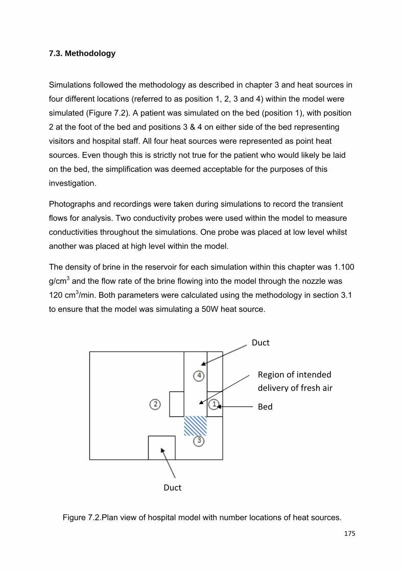
175
7.3. Methodology
Simulations followed the methodology as described in chapter 3 and heat sources in
four different locations (referred to as position 1, 2, 3 and 4) within the model were
simulated (Figure 7.2). A patient was simulated on the bed (position 1), with position
2 at the foot of the bed and positions 3 & 4 on either side of the bed representing
visitors and hospital staff. All four heat sources were represented as point heat
sources. Even though this is strictly not true for the patient who would likely be laid
on the bed, the simplification was deemed acceptable for the purposes of this
investigation.
Photographs and recordings were taken during simulations to record the transient
flows for analysis. Two conductivity probes were used within the model to measure
conductivities throughout the simulations. One probe was placed at low level whilst
another was placed at high level within the model.
The density of brine in the reservoir for each simulation within this chapter was 1.100
g/cm3 and the flow rate of the brine flowing into the model through the nozzle was
120 cm3/min. Both parameters were calculated using the methodology in section 3.1
to ensure that the model was simulating a 50W heat source.
Figure 7.2.Plan view of hospital model with number locations of heat sources.
Region of intended
delivery of fresh air
Duct
Bed
Duct
176
7.4 Results and discussion
Initial simulations were conducted with the heat source at position 1 or 2 to ensure
that the model was correctly working. The development of flows within these initial
simulations are described and compared with CFD simulations. The development of
internal converted densities at high and low level are then compared between the 4
heat source locations for both filling and draining simulations.
7.4.1 Observed flow behaviour
Initially, the model is filled with ambient fluid, both openings are opened and at t = 0s,
the brine source at position 2 (foot of the bed) is turned on. Brine flowed out of the
nozzle fully turbulent, resulting in the brine plume entraining ambient fluid (fresh
water). The brine plume reached the bottom of the model and began to horizontally
spread outwards (Figure. 7.3a). The brine at the bottom of the model began to build
up (Figure. 7.3b) to a point where an interface began to form (Figure. 7.3c).
After the interface fell below the duct opening (Figure 7.3d), the converted density at
low level below the interface began to increase beyond ambient. This occurred
because the inlet duct was above the interface, resulting in the incoming ‘fresh’ water
mixing with the brine above the interface, before flowing into the space near the bed.
Steady state was reached when the interface reached approximately 9cm. This
means that for a real hospital room using this ventilation technique, the fresh air is
pre-warmed before coming into contact with the patient, reducing the chance of
thermal discomfort due to droughts, while also potentially reducing heating
requirements during winter.
However, this mixing of incoming air with warm air at high level within the space may
increase the risk of infection to patients within the space if the ventilation system is
used for rooms with more than one patient. The intention of the incoming air to flow
onto the patient is to reduce air from other patients in the form of coughs and
sneezes being breathed in by the patient due to positive air pressure in the vicinity
around the patient. However, because the incoming air mixes with air that may
177
contain particulates from other patient's coughs and sneezes, it becomes possible
for another patient to become infected. To prevent this, the duct height must be
reduced such that it is below the interface. However, the trade-off will be increased
heating requirements and potential for thermal discomfort with droughts.
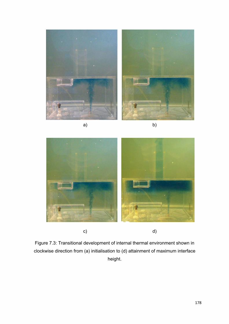
178
a) b)
c) d)
Figure 7.3: Transitional development of internal thermal environment shown in
clockwise direction from (a) initialisation to (d) attainment of maximum interface
height.
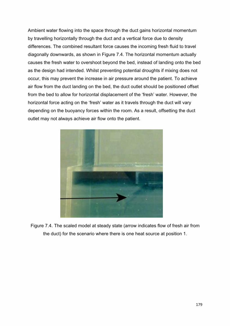
179
Ambient water flowing into the space through the duct gains horizontal momentum
by travelling horizontally through the duct and a vertical force due to density
differences. The combined resultant force causes the incoming fresh fluid to travel
diagonally downwards, as shown in Figure 7.4. The horizontal momentum actually
causes the fresh water to overshoot beyond the bed, instead of landing onto the bed
as the design had intended. Whilst preventing potential droughts if mixing does not
occur, this may prevent the increase in air pressure around the patient. To achieve
air flow from the duct landing on the bed, the duct outlet should be positioned offset
from the bed to allow for horizontal displacement of the ‘fresh’ water. However, the
horizontal force acting on the ‘fresh’ water as it travels through the duct will vary
depending on the buoyancy forces within the room. As a result, offsetting the duct
outlet may not always achieve air flow onto the patient.
Figure 7.4. The scaled model at steady state (arrow indicates flow of fresh air from
the duct) for the scenario where there is one heat source at position 1.
180
7.4.2 Comparison with CFD
Experimental and CFD simulations are compared for the scenario where the only
heat source in the room is a patient on the bed (scenario 1). The CFD simulation
modelled full scale with a 50W heat source. This comparison intends to aide in the
validation of both simulation techniques. The interface height in the Perspex model
was approximately 13cm at steady state, with CFD simulations (Figure 7.5) and the
analytical model described in Chapter 3 in close agreement (with h/H = 0.52 and
0.54 respectively).
When the heat source is at position 1, the interface height remains above the duct
opening where fresh fluid flows into the room for the patient scenario. This would
mean that incoming ambient water should not be pre-warmed as it enters the space.
However, a build-up of brine (in WBM) and hot air (CFD) is observed (Figure 7.6)
behind the duct. This build up caused the fluid to flow over the duct opening causing
pre-warming of the incoming ambient fluid. Close agreement between CFD and
WBM for interface heights and the building up of brine provides confidence for both
simulation techniques, even for complicated ventilation designs.
As a result, the fluid flowing into the room from the vent mixed with the overflowing
brine/hot air, causing the region below the interface to become warmer than ambient.
Future ventilation designs could attempt to incorporate designs which allow for hot
air to build up around and flow over an inlet to ‘pre-warm incoming cold air.

181
Figure 7.5: The interface layer in (a) WBM and (b) CFD equivalent.
Figure 7.6: Formation of build up of fluid around the duct in (a) CFD and (b) WBM .
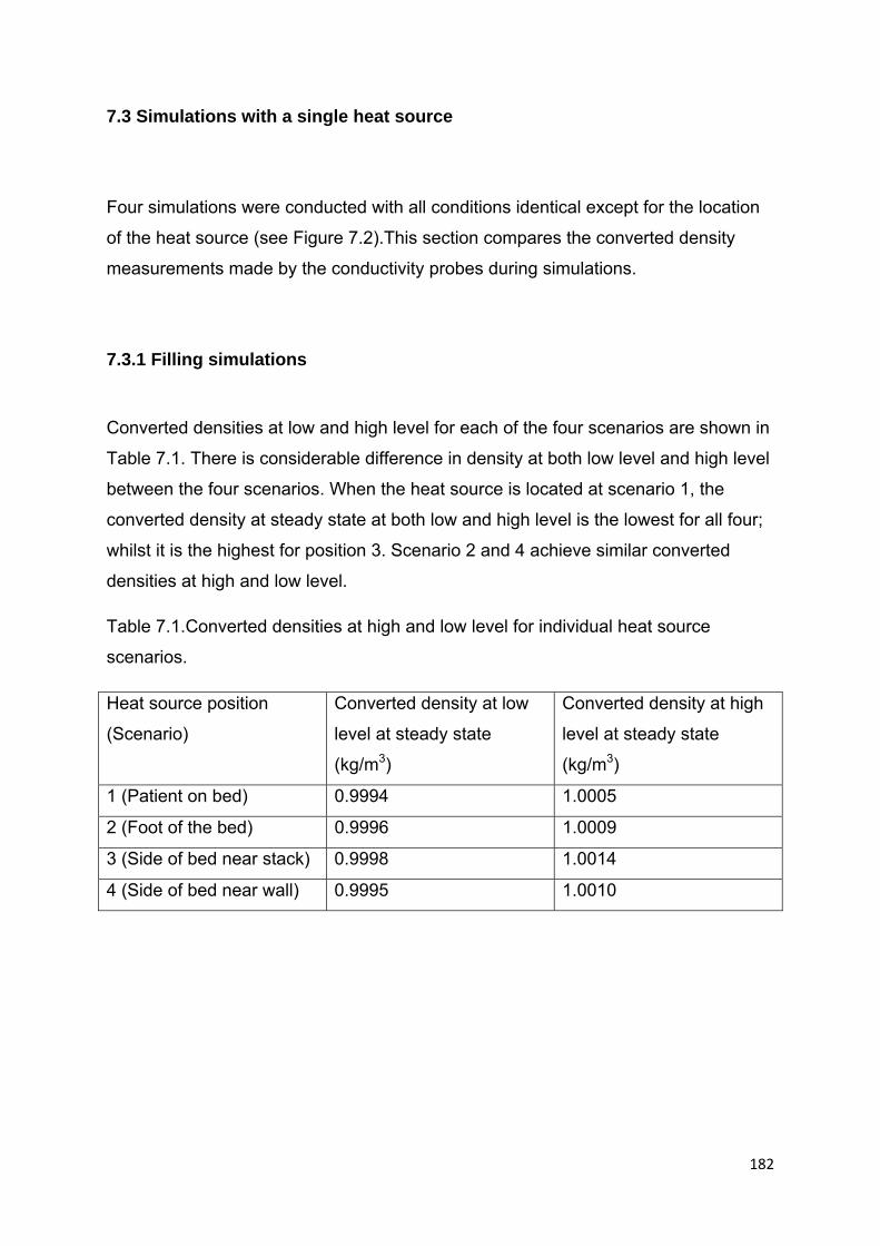
182
7.3 Simulations with a single heat source
Four simulations were conducted with all conditions identical except for the location
of the heat source (see Figure 7.2).This section compares the converted density
measurements made by the conductivity probes during simulations.
7.3.1 Filling simulations
Converted densities at low and high level for each of the four scenarios are shown in
Table 7.1. There is considerable difference in density at both low level and high level
between the four scenarios. When the heat source is located at scenario 1, the
converted density at steady state at both low and high level is the lowest for all four;
whilst it is the highest for position 3. Scenario 2 and 4 achieve similar converted
densities at high and low level.
Table 7.1.Converted densities at high and low level for individual heat source
scenarios.
Heat source position
(Scenario)
Converted density at low
level at steady state
(kg/m3)
Converted density at high
level at steady state
(kg/m3)
1 (Patient on bed) 0.9994 1.0005
2 (Foot of the bed) 0.9996 1.0009
3 (Side of bed near stack) 0.9998 1.0014
4 (Side of bed near wall) 0.9995 1.0010

183
a)
b)
Figure 7.7. Filling simulations for scenarios where individual heat sources are within
the space where a) density recorded at high level and b) density recorded at low
level.
‐0.2
0
0.2
0.4
0.6
0.8
1
1.2
1.4
0 200 400 600 800 1000 1200 1400
Norm
alised converted density
Time (s)
1
2
3
4
0
0.5
1
1.5
2
2.5
3
0 200 400 600 800 1000 1200 1400
Norm
alised converted density
Time (s)
1
2
3
4
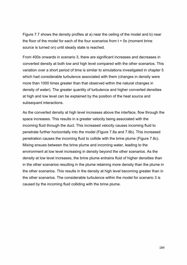
184
Figure 7.7 shows the density profiles at a) near the ceiling of the model and b) near
the floor of the model for each of the four scenarios from t = 0s (moment brine
source is turned on) until steady state is reached.
From 400s onwards in scenario 3, there are significant increases and decreases in
converted density at both low and high level compared with the other scenarios. This
variation over a short period of time is similar to simulations investigated in chapter 5
which had considerable turbulence associated with them (changes in density were
more than 1000 times greater than that observed within the natural changes in
density of water). The greater quantity of turbulence and higher converted densities
at high and low level can be explained by the position of the heat source and
subsequent interactions.
As the converted density at high level increases above the interface, flow through the
space increases. This results in a greater velocity being associated with the
incoming fluid through the duct. This increased velocity causes incoming fluid to
penetrate further horizontally into the model (Figure 7.8a and 7.8b). This increased
penetration causes the incoming fluid to collide with the brine plume (Figure 7.8c).
Mixing ensues between the brine plume and incoming water, leading to the
environment at low level increasing in density beyond the other scenarios. As the
density at low level increases, the brine plume entrains fluid of higher densities than
in the other scenarios resulting in the plume retaining more density than the plume in
the other scenarios. This results in the density at high level becoming greater than in
the other scenarios. The considerable turbulence within the model for scenario 3 is
caused by the incoming fluid colliding with the brine plume.
185
a) t = 0s b) t = 200s c) t = 650s
Figure 7.8.Development of flow characteristics for heat source location 3. The size
and direction of the blue arrow represents the relative strength and direction of
incoming ambient fluid.
There are two locations where the exchange in fluid across the interface in all four
simulations occurs. The first is the brine plume which penetrates the interface,
therefore increasing the density above the interface. The second occurs where the
incoming fresh water from above the interface mixes with denser than ambient fluid
above the interface before penetrating through the interface resulting in an increase
in density below the interface. As the density below the interface increases, the brine
plume entrains fluid of a greater density before penetrating the interface. This results
in the brine plume losing less density compared to a scenario where the fluid below
the interface has a density identical to ambient fluid. Because the brine plume has a
higher density when penetrating the interface, the density above the interface
increases. Due to mixing between the incoming fresh water and denser than ambient
fluid above the interface, the incoming water entrains fluid of greater density resulting
in a further increase to densities below the interface. Because of this two way
exchange of fluid, densities below and above the interface stabilise at the same time.
Scenario 1 has the lowest steady state density at both low and high level within the
model and takes up to 40% longer to achieve steady state than the other three
scenarios. During the simulation at 0 < t> 300s, converted densities at high level rise
at a rate similar to that in the other three scenarios reaching 1.0005 kg/m3 by 300s.
However, it takes another 700s to reach steady state densities at 1.00055kg/m3. This
period of small increase in density over a long period of time will be referred to as the
region of protraction, where the duration tp and density increase of the protracted
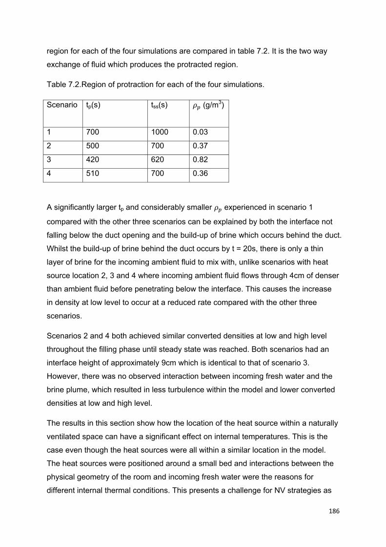
186
region for each of the four simulations are compared in table 7.2. It is the two way
exchange of fluid which produces the protracted region.
Table 7.2.Region of protraction for each of the four simulations.
Scenario tp(s)
tss(s)
(g/m3)
1 700 1000 0.03
2 500 700 0.37
3 420 620 0.82
4 510 700 0.36
A significantly larger tp and considerably smaller experienced in scenario 1
compared with the other three scenarios can be explained by both the interface not
falling below the duct opening and the build-up of brine which occurs behind the duct.
Whilst the build-up of brine behind the duct occurs by t = 20s, there is only a thin
layer of brine for the incoming ambient fluid to mix with, unlike scenarios with heat
source location 2, 3 and 4 where incoming ambient fluid flows through 4cm of denser
than ambient fluid before penetrating below the interface. This causes the increase
in density at low level to occur at a reduced rate compared with the other three
scenarios.
Scenarios 2 and 4 both achieved similar converted densities at low and high level
throughout the filling phase until steady state was reached. Both scenarios had an
interface height of approximately 9cm which is identical to that of scenario 3.
However, there was no observed interaction between incoming fresh water and the
brine plume, which resulted in less turbulence within the model and lower converted
densities at low and high level.
The results in this section show how the location of the heat source within a naturally
ventilated space can have a significant effect on internal temperatures. This is the
case even though the heat sources were all within a similar location in the model.
The heat sources were positioned around a small bed and interactions between the
physical geometry of the room and incoming fresh water were the reasons for
different internal thermal conditions. This presents a challenge for NV strategies as

187
the location of people within a space can be very transient. However it is possible to
take advantage of the interactions observed to achieve thermal environments which
ensure a more comfortable environment in NV buildings. The results also question
the applicability of this NV strategy during summer, where pre-warming of already
very warm ambient air may not lead to comfortable internal temperatures.
7.3.2 Emptying simulations
After the simulations reported in 7.3.1 reached steady state, the brine source is
turned off and the model then drains. Figure 7.9 shows the converted density graphs
for all four scenarios draining from steady state conditions, where a) is at high level
and b) is at low level. At t = 0s, the brine source in each simulation is turned off.
As shown in chapter 5, converted density profiles during draining can provide
significant insight into layers and their density profiles which exist at steady state
whilst a brine source is on.
For all four scenarios, there are three different layers within the model. The first layer
which drained during the first 100 seconds in all four scenarios was homogenous.
Initially, before the brine source is turned off, this first layers extent is from the
bottom of the duct upwards. The second layer which drained between 100 to 150s
(for scenarios 1, 2 and 4) and 100 to 300s (for scenario 3) sees a significant
reduction in density (approximately 50% of ) from the top of the layer to the bottom.
Initially, this layer was located from the interface to the bottom of the duct. From t =
0s, fresh water flows into the layer diluting layer 2. Because the brine source is
turned off, this layer significantly reduces in density during draining. From 150s
onwards, only the layer which was initially below the interface at t = 0s remains in the
model. Flow from the duct continues to mix and dilute this layer, causing an
extended period before the model has fully drained. Similar extended periods of
draining due to mixing is discussed in chapter 4.

188
i)
ii)
Figure 7.9.Converted densities at i) high level and ii) low level during the draining of
scenarios 1, 2, 3 and 4.
0
0.5
1
1.5
2
2.5
3
0 200 400 600 800 1000 1200 1400
Norm
alised converted density
Time (s)
1
2
3
4
Scenario
0
0.2
0.4
0.6
0.8
1
1.2
0 200 400 600 800 1000 1200 1400
Norm
alised converted density
Time (s)
1
2
3
4
Scenario

189
Interestingly, the time for the model to empty for each of the scenarios is
approximately the same. Equation 2.11 (Section 2.7.1) states that as the density
within the model increases, draining time will decrease. For each of the scenarios,
the density at t = 0s is different in the top layer. The greater the density in this layer,
the greater the flow through the space resulting in a larger volume of fresh water
flowing into the space. This causes increasing amounts of dilution in the bottom two
layers. Over time, the densities within the bottom two layers become equal across
the scenarios resulting in an identical time to drain. This means that it will not be a
quick process to completely ventilate the room using this ventilation design, which
could cause cross infection between patients, especially if there is a high turnover of
patients.
7.4 Summary of Benchmark 3
This chapter reported WBM simulations to investigate a novel ventilation strategy
which intends to reduce cross infection between patients. This involves a stack
which allows hot air to flow out of the room, with a high level duct allowing ambient
air to flow into the room. It is the intention of the design to have fresh air flowing
directly into the vicinity of the patient to create a positive air pressure to reduce cross
infection.
Importantly, this chapter sets out to further understand this ventilation technique and
four simulations were conducted, each with the brine source at a different location.
Densities were measured at high and low level within the model and it was shown
that with identical physical parameters between all simulations except the location of
the heat source, significant variation in internal densities at low and high level occurs.
The time to reach steady state within the model is also shown to vary. Such variation
is caused by the interaction between the brine plume and the duct or incoming fresh
water.
Agreement has been shown for the flow regimes within the model between CFD and
WBM simulations, which provides confidence in the simulation techniques.
190
For the scenario where a heat source is located such that direct interaction between
incoming fluid and the brine plume occurred, significantly higher internal
temperatures were observed at both low and high level. For the case where only the
patient is in the room, lowest internal temperatures were observed and this is
attributed to interface remaining above the duct. Interestingly, due to the location of
the duct, a build-up of brine behind the duct was observed which caused brine to
flow over the opening resulting in a mixed environment. This mixed environment
reduces heating requirements for the room as incoming fluid is pre-warmed.
However, the suitability for this strategy to reduce infection of patients is
questionable unless the height of the duct is reduced to ensure that mixing between
incoming fluid and stale air does not occur.

191
Chapter 8.Discussion Chapter
8.1. Preamble.
The purpose of this chapter is to discuss the implications of the experimental findings
of the previous three chapters for natural ventilation design and performance. The
latter part of the chapter refers to other models which were used during this research
with the intention to further improve our understanding of natural ventilation.
8.2. Discussion of results
8.2.1. Benchmark 1 (Simple model)
Chapters 4 and 5 discussed and analysed results from a cube shaped model
measuring 0.29 x 0.29 x 0.29m with openings on the floor, ceiling, and two opposite
sides. Hollow cylinders were fabricated such that they could slide into the openings
on the ceiling of the model to form stacks allowing for stack ventilation to also be
simulated. The simulations conducted can be categorised as ‘filling’ simulations or
‘emptying simulations.
8.2.1.1. Filling simulations within simple model
Filling simulations were all initially set up such that the model was filled with ambient
fluid and there was no brine flowing into the model. At time, t = 0s, the brine source
was turned on and one of several flow regimes began depending on the location of
the openings used during each simulation. In total, there were 4 different opening
location strategies simulated with several simulations conducted within a strategy
with varying number of openings (Figure 8.1). The location of the openings within
strategy 2 and 3 caused incoming fluid to collide with the hot air plume, resulting in a
disturbed plume. The resulting thermal environment caused by a disturbed plume is
further discussed later within this section.
192
Strategy 1: Openings on side (non-disturbed plume)
Strategy 2: Openings on side (disturbed plume)
Strategy 3: Openings on floor and ceiling
Strategy 4: Openings on floor and stacks on ceiling
Figure 8.1.Opening strategies for filling simulations used in Chapter 4 and 5.
Simulations following strategy 1 followed traditional displacement ventilation flow
which results in a layer of ambient temperature at low level, with an interface at high
level and a layer of warmer-than-ambient temperatures above the interface. Such a
193
strategy is useful when ambient temperatures are already warm. However care is
required to ensure that the interface height is above the occupants within the space
to avoid thermal discomfort.
At the time of writing the literature review for this research, work by others could not
be found which simulated strategies 2, 3 and 4.
The opening locations in strategy 2 are similar to those in strategy 1, except that the
lower openings are placed such that incoming ambient fluid collides with the brine
plume. Such interactions cause the temperature at low level to rise above ambient
levels, which will be an attractive solution when ambient temperatures are cool.
The theory discussed in Chapter 2 states that as the height difference between lower
and upper openings increases, the flow rate through the space increases, which
results in reduced internal temperatures and a higher interface. As a result, this
suggests that strategy 3 and 4 should produce a thermal environment which is more
attractive when ambient temperatures are warmer. However, incoming ambient fluid
had sufficient velocity that it penetrated the interface, dispelling warmer-than-ambient
fluid towards the floor, resulting in a mixed environment similar to ventilation strategy
2. However, low level temperatures were observed to be greater than that of
ventilation strategy 2 which would mean that ventilation strategies 3 and 4 were
suitable when ambient temperatures were cold. Interestingly, almost identical
temperatures at low level were observed between a ventilation strategy 2 simulations
using 2No. openings at low and high level and a ventilation strategy 4 simulation
using 4No. openings. This suggests that the location of the openings can have a
more significant impact on internal temperatures than opening area.
Care is required when applying the results from the filling simulations discussed
above to real world natural ventilation. This is because water bath modelling with
brine does not simulate gravity currents at the start of the model. Gravity currents
describe cool air flowing into a warmer space through an opening. As the air flows
into the space, the air becomes less buoyant due to it being cooler in temperature
and as a result, flows into the space whilst decreasing in height towards the floor.
This did not occur within the simulations as water external from the model was at the
same density as water within the model at near the floor. However, for a number of
simulations conducted, part way through the simulation, densities at low level began
194
to increase resulting in a density difference between incoming fresh water and the
low density brine near the floor of the model. In such cases, the incoming water was
not observed to flow to the floor of the model and this is likely due to the following
reasons. Firstly, when the openings were on the floor and ceiling, the velocity
associated with the incoming fresh water was sufficient to overcome any reduction in
buoyancy. Secondly, the velocity associated with the incoming fresh water resulted
in rapid mixing, resulting in the density of the incoming fluid tending towards the
buoyancy at low level.
8.2.1.2. Discussion of emptying simulations within simple model
For initial draining simulations, interface heights were measured with time and
results compared with theoretic predictions for traditional displacement flow regimes.
Close agreement was achieved until the interface height approached the upper
openings, when a significant reduction in draining rate occurred. It was found that
this was caused by a mixed layer below the interface, which comprised of a lower
temperature than the layer of fluid above the interface. Night purging ventilation
strategies rely upon openings to dispel built up heat within a room during periods
where the room is unoccupied (for example at night). If a mixed layer exists within
the space, then draining times will significantly increase (greater than double the
time required to drain), greatly diminishing the effectiveness of the purging strategy.
Ventilation strategy 1 simulations were observed to have relatively small mixed
layers, while ventilation strategies 2, 3 and 4 had significantly larger mixed layers.
The effect of the mixed layer is sufficient to ensure that a ventilation strategy 1
simulation with 2No. openings at low and high level achieved a faster draining time
than ventilation strategies 3 and 4 with 4No. openings at low and high level.
8.2.2. Benchmark 2 (Open plan office)
Three different flow regimes were confirmed to exist for a model with a single low
level opening and 2No. stacks of different lengths (Figure 8.2). Varying the lower
opening area dictates which of the three flow regimes develops when brine begins to

195
flow into the model and depending on the size of the lower opening, it is possible to
force the flow regime to change to one or both other flow regimes. This was
achieved by simulating fans which could eject warmer-than-ambient fluid from within
the model to flow out of the stack, or force ambient fluid to flow into the stack. The
simulated fans were required to inject or expel a specific volume of fluid which
equated to between 10 and 20% of the stack volume to change the flow regime. The
simulated fans can then be turned off, allowing natural ventilation to drive the flow
through the space without the flow regime reverting back to the previous flow regime.
Regime i) Regime ii) Regime iii)
Figure 8.2. Three possible flow regimes for model used in Chapter 6.
When steady state was reached for each of the three flow regimes, varying internal
temperatures and flow patterns existed. Regime ii) followed traditional displacement
ventilation whilst i) and iii) had mixed environments, with Regime iii) achieving the
highest temperatures at both low and high level.
A naturally ventilated building using this stack strategy with automated fans is an
effective method of changing the flow regime of a space to decrease or increase
temperatures at low level, adapting to different heat loads and ambient temperatures.
8.2.3. Benchmark 3 (Hospital ward)
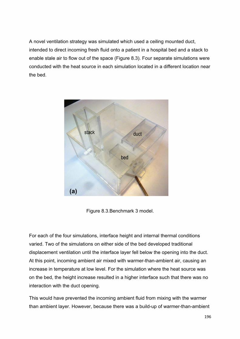
196
A novel ventilation strategy was simulated which used a ceiling mounted duct,
intended to direct incoming fresh fluid onto a patient in a hospital bed and a stack to
enable stale air to flow out of the space (Figure 8.3). Four separate simulations were
conducted with the heat source in each simulation located in a different location near
the bed.
Figure 8.3.Benchmark 3 model.
For each of the four simulations, interface height and internal thermal conditions
varied. Two of the simulations on either side of the bed developed traditional
displacement ventilation until the interface layer fell below the opening into the duct.
At this point, incoming ambient air mixed with warmer-than-ambient air, causing an
increase in temperature at low level. For the simulation where the heat source was
on the bed, the height increase resulted in a higher interface such that there was no
interaction with the duct opening.
This would have prevented the incoming ambient fluid from mixing with the warmer
than ambient layer. However, because there was a build-up of warmer-than-ambient

197
fluid behind the duct. This built up layer of warmer-than-ambient fluid began flowing
over the duct opening and mixing was able to occur. For the case where the brine
source was located on the side of the bed furthest from the duct, incoming ambient
fluid collided with the plume from the simulated heat source, resulting in significant
mixing at low level which resulted in the greatest temperatures at both low and high
level.
8.2.4. Natural ventilation design implications
The small driving forces associated with NV buildings will often result in large
opening areas to ensure sufficient flow rates to prevent overheating. The
practicalities of such large opening areas are not always possible for buildings,
resulting in air conditioning being used instead of an NV strategy. This results in an
increase in energy usage and importantly, an increase in carbon equivalent
emissions.
When sufficiently large opening areas are achieved within an NV strategy, internal
temperatures can still become warmer than theoretical assumptions under certain
circumstances. These can include interactions between incoming ambient fluid and a
heat source plume or wind overpowering the NV driving forces, both examples result
in different internal temperatures which may cause occupants to experience
discomfort. Uncomfortable thermal conditions within a NV building may result in
occupants and building owners having a negative perspective of natural ventilation,
which may further increase the usage of air conditioning within buildings.
Importantly, this research has shown that different NV strategies within a water bath
model can result in very different internal thermal environments. Certain strategies
can achieve comfortable internal temperatures with considerably smaller opening
areas, suggesting that building designers need to carefully select the most suited NV
strategy.
Once an NV building is constructed, it is often expensive and difficult to change the
NV strategy or increase the opening area. Ensuring that there is flexibility is
important to ensure a more thermally comfortable space. Traditionally, this has
involved windows which can be opened by varying degrees ensuring that occupants

198
can vary the amount of ventilation to the space. This will result in increases or
decreases in internal temperatures, however may cause cold droughts during winter.
Positioning openings such that incoming ambient fluid is pre-heated by warmer than
ambient air within the room reduces the risk of cold droughts whilst also reducing
heating requirements. Interestingly, this research suggests that it may be possible to
mechanically force different flow regimes to ensure thermally comfortable internal
conditions with both varying external temperatures and number of people/internal
heat gains. This could ensure that NV buildings can be adaptive to the often flexible
occupancy
8.3. Other models
In addition to the three models described in chapters 4, 5, 6 and 7, the research
looked at two other models in order to further understand mechanically forcing
specific flow regimes and complicated interactions between geometry and heat
sources within a NV building.
8.3.1. Benchmark 2 with a distributed heat source.
Chenvidyakarn and Woods (2004) reported on a model with a distributed heat
source and showed that it was possible for multiple flow regimes to occur. Their
simulations were conducted within a water bath using heated wires to simulate a
heat source. A model was fabricated with a sintered bronze plate (see 2.7.2.6),
initially to determine if multiple flows could also occur within water bath modelling
using brine to simulate a heat source.
The sintered bronze plate used to simulate the distributed heat source closely
followed theoretic predictions, at steady state, the space was filled with warmer than
ambient fluid. By varying the lower opening area and simulating wind, three different
flow regimes were observed. Further simulations were conducted to analyse the
effect on the internal thermal environment when the lower opening position is varied

199
and the consequences to the emptying of the space. However, limitations with the
sintered bronze plate prevented sufficient simulations for further analysis. This was
due to algae forming within the bronze plate which over time reduced the volume
flow rate of brine which could flow through the plate. After several simulations,
sufficient quantity of algae was present that even with the use of a pump, brine could
not be pumped through the plate. The high price of a bronze sintered plate (approx.
£150 per sheet) meant that it was not feasible to run further simulations with new
sintered bronze plates.
8.3.2 Benchmark 4 (Theatre)
Originally, it was intended for this research to discuss four benchmarks, with the
fourth consisting of a highly complicated theatre model (Figure 8.4). Involving over
100 nozzles on raked seating, the model was complex,taking over 6 months to
construct. Initial simulations showed highly promising results, with varying flow
regimes caused by the location of heat sources around the space resulting in poor
ventilation in certain areas of the model. For example, when occupants were located
on the lower seating tier, brine flowed onto the upper seating tier, resulting in the
exposure of stale warm air which would reduce thermal comfort and health. Brine
from the stage heat sources were also shown to flow onto the upper seating area.
Stage Lower seating tier Upper seating tier
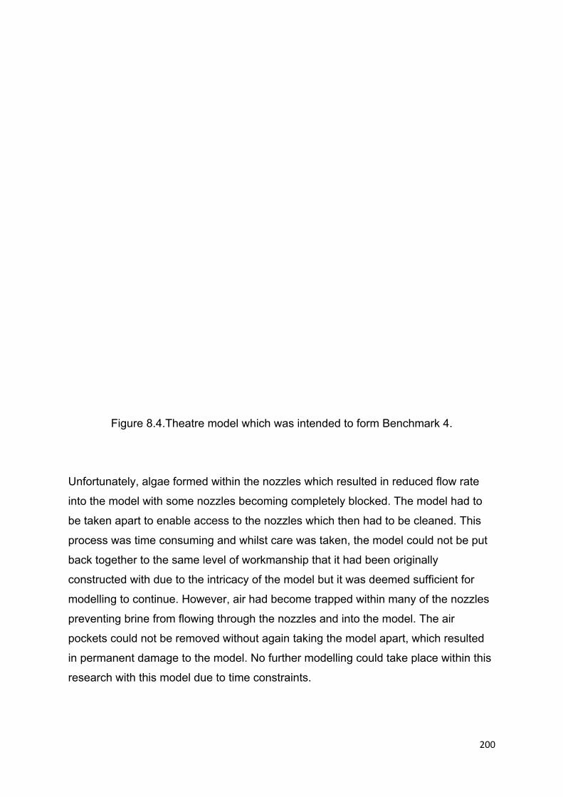
200
Figure 8.4.Theatre model which was intended to form Benchmark 4.
Unfortunately, algae formed within the nozzles which resulted in reduced flow rate
into the model with some nozzles becoming completely blocked. The model had to
be taken apart to enable access to the nozzles which then had to be cleaned. This
process was time consuming and whilst care was taken, the model could not be put
back together to the same level of workmanship that it had been originally
constructed with due to the intricacy of the model but it was deemed sufficient for
modelling to continue. However, air had become trapped within many of the nozzles
preventing brine from flowing through the nozzles and into the model. The air
pockets could not be removed without again taking the model apart, which resulted
in permanent damage to the model. No further modelling could take place within this
research with this model due to time constraints.
201
Benchmark 4 pushed the boundaries of Water Bath Modelling with the use of brine,
although it is recommended that if future research is conducted on Benchmark 4,
that brine is not used and instead, electric filaments are used to produce density
differences within the model. The use of electric filaments instead of brine will have
the advantage that there will be no nozzles, preventing the issues of air pockets and
algae.
202
Chapter 9. Conclusions and suggestions for further work
9.1. Conclusions from this work
Low energy solutions to our everyday needs have become increasingly important
with increased understanding of global warming. UK and European legislation is
updated every few years to encourage building designers to ensure that the
buildings they design use increasingly less energy. Natural ventilation offers a low
energy alternative to mechanical ventilation and air conditioning for the control of
internal temperatures and pollutants.
This work was concerned with the application of natural ventilation as a strategy to
achieve a thermally comfortable internal environment. The aims of this research can
be split into two: firstly to design and build a water bath facility and show agreement
with existing theory and secondly, to use the facility to compare the effect of opening
strategies on the thermal environment and simulate time dependent flows.
A water bath modelling facility was constructed and simple simulations were run
which demonstrated that there was close agreement between experimental,
theoretical and observations from other researchers for interface heights, flow
regimes and internal temperatures. Such close agreement provided confidence that
the WBM facility modelled natural ventilation accurately and allowed for more
complicated simulations to be conducted.
This research provides some guidance for building designers by demonstrating the
effect that different opening strategies has on internal temperatures, flow regimes
and energy use within a space. This will help ensure that the correct opening
strategy for a naturally ventilated space will be selected, reducing the risk of thermal
discomfort whilst also increasing the use of natural ventilation and minimising
mechanical ventilation and air conditioning.
Firstly, building designers must select whether a displacement or mixed natural
ventilation strategy provides a more favourable thermal environment. The former
ensures that ambient air is at low level and hot air is at high level whilst the latter has
a thermal environment which is warmer than ambient throughout. A displaced
203
thermal environment is well suited to ventilating a space when ambient temperatures
are high (i.e. during summer), whilst a mixed environment is most effective in winter
by reducing the requirement for heating. Both thermal environments are achieved
primarily with different opening strategies. It is apparent that a trade off is required
when a naturally ventilated space is designed: building designers will have to
determine whether cooler temperatures at low level in summer or smaller heating
requirements in winter is a priority. A space with substantial heat gains will likely
require less heating during winter, but thermal comfort of occupants will significantly
improve during summer with a displacement ventilation strategy. The opposite is true
for a space with small heat gains, where differences between ambient and internal
temperatures are much smaller during summer, but substantial savings in heating
can be made in winter.
Secondly, the position of openings and the potential use of stacks must be carefully
considered to ensure that the desired thermal environment is achieved (Chapter 4).
If openings are placed on the floor of a room or if stacks are used, it is likely that a
mixed thermal environment will occur. Whereas a displacement thermal environment
will likely occur when the openings are placed on the walls of the room. Stacks are
often used by building designers to increase air flow into a space compared to a
cross ventilated strategy with the intention of reducing internal temperatures.
However stacks have been shown to cause a mixed thermal environment, resulting
in greater temperatures at low levels than cross ventilated spaces.
Thirdly the position of any heat sources within a space should be carefully
considered. Incoming ambient air from an opening may collide within a hot air plume,
resulting in a thermally mixed environment. This poses considerable difficulty with
building designers as the location of heat sources is unlikely to be fixed throughout
the lifetime of a building.
Fourthly, building designers will have to ascertain whether a night time draining
strategy is required to cool any thermal mass within a room. The draining of a
naturally ventilated space with a mixed thermal environment takes more than double
the amount of time to reach ambient temperatures compared with the draining of a
displaced thermal environment. This could prevent any thermal mass being fully
204
recharged, resulting in a space becoming warmer and warmer throughout the
summer.
Finally, interactions between resulting heat plumes and the geometry of a space
must be considered if high level openings are used to allow fresh air to flow into a
space (Chapter 6). It has been shown that in specific cases, warmer than ambient air
can build up in localised regions around the fresh air inlet, resulting in a mixed
thermal environment instead of displacement occurring.
An experimental ventilation technique was demonstrated which was able to produce
both a displaced and mixed thermal environment within a room by taking advantage
of time dependent flows (Chapter 7). This was achieved by using intermittent
temporary fans within the stacks of a room which would be controlled by temperature
sensors. The energy requirements of the intermittent fans and temperature sensors
would be very small in comparison to the energy costs of a mechanical or air
conditioned system. Such a design enables larger spaces with high heat gains to
become naturally ventilated with displacement ventilation during summer, whilst in
winter, a mixed mode ventilation strategy saves considerable energy in heating.
9.2. Future work
Initial simulations of raked-seat auditoriums with stacks provided insight into time
dependent flows which were dictated by the location of the heat sources. However,
the complex nature of the model prevented a complete analysis. Instead of
simulating a heat source with brine, heated wires could be used. The results from
this will likely provide a stronger understanding of time dependant flows and also
show how flow regimes form within a complicated NV space.
Further analysis of the resulting thermal environment and flow regimes with different
opening locations whilst controlling time dependent flows is required. This will further
our understanding of the most effective strategies for ensuring thermally comfortable
conditions in large spaces with large heat gains whilst reducing heating requirements.
The control mechanism for controlling time dependent flows is also required to
produce a working prototype. This would likely consist of internal and temperature
205
sensors along with automatic controlled louvres at low and high level, with the ability
to determine which flow regime would most likely achieve the greatest thermal
comfort for occupants within the space.
Within Chapter 3, poorly ventilated zones were briefly discussed. Simulating different
ventilation strategies and determining any dead spaces will highlight any poorly
ventilated areas within a space. This will lead to further research on how to reduce,
and if possible eliminate such zones.
Further comparisons between CFD and water bath modelling would work towards
providing further confidence in the results of both simulating techniques, of particular
interest is whether gravity currents occur in the CFD model at times when within the
water bath, it does not even though there is a density difference between the fluid at
low level in the model and incoming fluid with a high associated velocity.
This work has shown that different entrainment values can be used to ensure close
theoretical agreement with interface heights and internal densities. Further
investigation is required to ascertain if more understanding is required in this area of
research.
9.3 Limitations of the work
Water Bath Modelling (WBM) is a physical modelling technique. As a result,
breakages should be expected and did invariably occur during this research. These
included nozzles becoming filled with algae, sensors failing and even models
breaking. Whilst the replacement or cleaning of the nozzles was a quick process,
replacement of sensors and repairing of models was time consuming and in some
cases expensive.
The natural ventilation equations within Chapter 2 do not account for heat loss
through the fabric or the additional heating within a space due to radiation which is
emitted by most heat sources. If brine is used to model a heat source within WBM,
there is no simple way to model heat loss through the fabric or radiation and as a
result, neither of these were modelled within this research. It should be noted that
206
other researchers who use Brine within WBM do not take these factors into account.
As buildings become increasingly insulated, the effect that heat losses have on the
thermal conditions within a space is reduced and therefore reduces the importance
of this limitation on WBM. As discussed in Chapter 2, not simulating the radiant heat
within a space is likely to result in a marginally increased interface height. This will
not have an impact on results unless interactions between the interface and the
geometry of the space leads to different thermal environments (see Chapter 7).
Assuming a displacement ventilation strategy, fresh water occupies the area within
the model below the interface and is of the same density as the fresh water flowing
into the model from the lower opening(s). At full scale, air flowing into the model is
usually more dense (cooler) than air within the room at low level. This can result in
what is referred to as density currents, where the incoming, denser fluid flows
towards the floor due to its decreased buoyancy. Further investigation is required to
ascertain whether this has any significant effect on results within water bath
modelling.

207
References
Adamu ZA, Cook MJ, Price ADF (2011). Natural Personalised Ventilation: A novel
approach, International Journal of Ventilation, 10(3): 263-275.
Adelaidehydronicheating, If it ain't broke, don't fix it.
http://www.adelaidehydronicheating.com.au/boilers.html[Accessed March 2011]
Akimoto T, 2009, Thermal comfort and productivity – Evaluation of workplace
environment in a task conditioned office. Building and Environment 45.1 45 - 50
Allocca C, Qingyan Chen and Glicksman LR 2003. Design analysis of single-sided
natural ventilation. Energy and Buildings 35 785-795
Andersen K. T, 2007. Airflow rates by combined natural ventilation with opposing
wind – umambiguous solutions for practical use. Building and Environment 42534 -
542
Andersen K. T, 2003.Theory for natural ventilation by thermal buoyancy in one zone
with uniform temperature. Building and Environment 38 (2003) 1281 - 1289
ASHRAE Standard 55 2004. Thermal environment conditions for human occupancy.
American Society of Heating, Refrigerating and Air-conditioning Engineers.
Awbi H.B. (2003) Ventilation of Buildings, Second Edition, 2003, ISBN 0415270553,
Taylor and Francis (E&FN Spon).
BBC 2006, Buildings and climate policy [Online].
www.news.bbc.co.uk/1/hi/sci/tech/4837008.stm [Accessed March 2011]
BBC 2010, ‘Paltry’ Copenhagen carbon pledges point to 3C world [Online].
http://news.bbc.co.uk/2/hi/science/nature/8635765.stm [Accessed April 2010]
BBC 2011a, Romans: technology [Online].
www.bbc.co.uk/schools/primaryhistory/romans/technology/ [Accessed January 2011]
BBC 2011b, Facebook shares green data centre technology [Online].
http://www.bbc.co.uk/news/technology-13010766 [Accessed April 2011]
208
Becker R, Goldbergera I, Paciuk M, 2006. Improving energy performance of school
buildings while ensuring indoor air quality ventilation. Building and Environment 42
3261-3276
Bolster D, Maillard A, Linden PF, 2008.The response of displacement ventilation to
time-varying heat sources. Energy and Buildings 40 2009-2110
Bolster D. T, Linden P. F, 2007. Contaminants in ventilated filling boxes.Journal of
Fluid mechanics. Vol 591, pp. 97-116..
Bordass W. T, Bormley A. K. R. and Leaman A. J. 1996. Comfort, control and energy
efficiency in offices, BSRIA IP395 (London construction Research Communications)
Bower D. J, Caulfield C. P, Fitzgerals S. D, Woods A. W, 2008. Transient ventilation
dynamics following a change in strength of a point source of heat. J. Fluid Mech.
(2008), vol 614, pp 15-37.
Brager G. S, and Dear R. J. de, 1998. Thermal adaption in the build environment: A
literature review. Energy and Buildings 27 83 - 96
Breathing Buildings 2014 http://www.breathingbuildings.com/home website
[Accessed June 2014]
Bouzinaoui A, Devienne R and Fontaine J 2007 An experimental study of the
thermal plume developed above a finite cylindrical heat source to validate the point
source model Experimental Thermal and Fluid Science, Volume 31, Issue 7, July
2007, Pages 649-659
Busch J.F, 1992. A tale of two populations: Thermal comfort in air- conditioned and
naturally ventilated offices in Thailand. Energy and Buildings 18(3-4):235 - 249
Candido C, Dear R. de, Lamberts R, Bittencourt L, 2008. Natural ventilation and
thermal comfort.Air movement acceptability limits and thermal comfort in Brazil’s hot
humid zone. 5th Windsor Conference: Air-Conditioning & The Low Carbon Cooling
Challenge, London: Network for Comfort and Energy Use in Buildings.
209
Castle Cover , the changing costs of utility prices in the UK
http://www.castlecover.co.uk/historic-home-utility-prices/ accessed April 2012
Chen, Q. (2009) Ventilation performance prediction for buildings: a method overview
and recent applications, Building and Environment, 44 (4), pp. 848–858
Chenvidyakarn T, Woods A, 2007. Stratification and oscillations produced by pre-
cooling during transient natural ventilation. Building and Environment 42 99–112
Chenvidyakarn T, Woods A, 2005. Multiple steady states in stack ventilation.
Building and Environment 40 399 - 410
Cho T.T, Fong K. F, Givoni B, Lin Z, Chan A. L. S, 2010. Thermal sensation of Hong
Kong people with increased air speed and humidity in air conditioned environment.
Building and Environment 45, issue 10 (2177-2183)
Chui Y. H, Etheridge D. W, 2004. Experimental technique to determine unsteady
flow in natural ventilation stacks at model scale. Journal of Wind Engineering and
Industrial Aerodynamics 92 291-313
CIBSE Guide A 2007, Environmental Design: CIBSE Guide a. 7th Edition. London:
The chartered institution of Building services Engineers. ISBN: 1903287669
CIBSE Guide C, 2007, Reference Data. Butterworth-Heinemann
CIBSE Guide F: Energy Efficiency in Buildings NEW 2012 ISBN 9781906846220
CIBSE TM40: 2006, Health issues in building services. London: The Chartered
Institution of Building Services Engineers.
Collet da Graça V.A, Kowaltowskia D. C. C. K, and Petreche J. R. D 2005. An
evaluation method for schoolbuilding design at the preliminary phase with
optimisation of aspects of environmental comfort for the school system of the State
São Paulo in Brazil. Building and Environment 42 984 - 999.
Cook MJ, 1998, An Evaluation of Computation Fluid Dynamic for Modelling
Buoyancy-Driven Displacement Ventilation [PhD thesis]

210
Cook M. J, 2009, Physical modelling [Lecture]. Advanced airflow modelling
09CVP311, Loughborough University, Civil and Building department, 11 December
2009
Cooper P, and Linden P.F, 1996.Natural ventilation of an enclosure containing two
buoyancy sources. J. Fluid mech, vol. 311, pp. 153-176
Dalziel S. B,1993. Rayleigh-Taylow instability: experiments with image analysis.
Dynamics of Atmospheres and Oceans, Volume 20, Issues 1-2, 30, Pages 127-153
Dalziel S. B, Lane-Serff G. F, 1991. The hydraulics of doorway exchange flows.
Building and environment, Vol 26, No. 2, pp 121-135.
Davidhazy A. no date, [online] Available at: http://people.rit.edu/andpph/text-schlieren.html). [Accessed October 2012]
Dear R. J. de, Leow K. G, Ameen A, 1991. Thermal comfort in the humid tropics –
part 1: Climate chamber experiments on temperature preferences in Singapore. Part
2: Climate chamber experiments on thermal acceptability in Singapore. ASHRAE
Transactions, 97 (1) 874-879, 880-886.
DECC 2011, Department of Energy and climage change, What is climate change?
[Online].
www.decc.gov.uk/en/content/cms/what_we_do/change_energy/what_is_cc/What_is_
cc.aspx [Accessed January 2011]
Department for Communities and Local Government 2013, Improving energy
efficiency of buildings and using planning to protect the environment.
https://www.gov.uk/government/policies/improving-the-energy-efficiency-of-buildings-
and-using-planning-to-protect-the-environment/supporting-pages/energy-
performance-of-buildings. [Accessed December 2013]
Designing Quality Learning Spaces: Heating & Insulation BRANZ 2007
Devienne R and Fontaine J, 2012 Experimental characterisation of a plume above
rectangular thermal sources. Effect of aspect ratio Building and Environment,
Volume 49, Pages 17-24

211
M. Economidou, G.R. Hunt 2010 Transient flows in enclosures: A generalised
approach for modelling the effects of geometry, heat gains and wind Original
Research Article Building and Environment, Volume 45, Issue 12, Pages 2607-2619
Energy Saving Trust, Energy efficient ventilation in dwellings – a guide for specifiers
2006
Energy Saving Trust, Energy efficient ventilation in dwellings – a guide for specifiers
2006. Can be downloaded from: http://www.beama.org.uk/en/publications/sector-
publications/index.cfm/GPG268
Energy Consumption Guide 19, 1993, Energy Efficiency in Offices, Energy Efficiency
Office/HMSO, London,
ESRL - Earth System Research Laboratory, Trends in Atmospheric Carbon Dioxide
[Online]. www.esrl.noaa.gov/gmd/ccg/trends/ [Accessed March 2011]
Etheridge D and Sandberg M 1996.Building Ventilation: Theory and Measurement.
Chichester, John Wiley and Sons, Inc
Etheridge D, Sandberg M A simple parametric study of ventilationOriginal Research
Article Building and Environment, Volume 19, Issue 3, 1984, Pages 163-173
Evola G. and Popov V, 2006.Computational analysis of wind driven natural
ventilation in buildings. Energy and Buildings 38 491 – 501.
Feriadi H, Wong N.H, Chandra S, Cheong K.W,2003. Adaptive behaviour and
thermal comfort in Singapore’s naturally ventilated housing. Building Research and
Information.
Fitzgerald, Shaun (2013), The science of Water Bath Modelling. Last accessed on
20/11/2013.http://www.breathingbuildings.com/news/natural-ventilation-blog/the-
science-of-water-bath-
modelling?utm_medium=email&utm_campaign=Breathing%20Buildings%20Septem
ber%202013&utm_content=Breathing%20Buildings%20September%202013+CID_9
d693cdd4307adef29f957cd77df241d&utm_source=CplusNewsletter [Accessed
December 2013]
212
Fitzgerald, SD and Woods, AW (2010) Transient natural ventilation of a space with
localised heating. BUILD ENVIRON 45 (12): 2778-2789 DEC 2010
Fitzgerald S. D, Woods A. W, 2008. The influence of stacks on flow patterns and
stratification associated with natural ventilation. Building and Environment 43 (2008)
1719-1733
Fitzgerald SD and Woods, AW (2007) On the transition from displacement to mixing
ventilation with a localized heat source. BUILD ENVIRON 42 (6): 2210-2217 JUN
2007
Fitzgerald S. D, Woods A. W, 2003. Natural ventilation of a room with vents at
multiple levels. Building and Environment 39 (2004) 505 – 521
Gangoiti G, Sancho J, Ibarra G, Alonso L, Garcia J. A, Navoza M, Durana N and
Ilardia J.L, 1997. Rise of moist plumes from tall stacks in turbulent and stratified
atmospheres. Atmospheric Environment, Volume 31, Issue 2, January 1997, Pages
253-269
Gladstone C, and Woods AW, 2001. On a buoyancy-driven natural ventilation of a
room with a heated floor. J. Fluid Mech. (2001), vol. 441, pp. 293{314.
Gladstone C, and Woods AW, 2001. On a buoyancy-driven natural ventilation of a
room with a heated floor. J. Fluid Mech, vol. 441, pp. 29
Heiselberg P, Li Y, Anderson A, Bjerre M, Chan Z, 2004, Experimental and CFD
evidence of multiple solutions in a naturally ventilation building. Indoor Air; 14: 43-54
Holford JM and Hunt GR 2003. Fundamental atrium design for natural ventilation.
Building and Environment 2003;38:409–26.
Hughes BR, Cheuk-ming M, 2011. A study of Wind and Buoyancy Driven Flows
through commercial wind towers. Energy and Buildings,
doi:10.1016/j.enbuild.2011.03.022 [Accepted Manuscript]
Humpreys M. 1978. Outdoor temperatures and comfort indoors.Building Research
and Practice, Vol 6. No. 2, pp. 92-105

213
Hunt G. R and Coffey, C. J. Emptying boxes – classifying transient natural ventilation
flows, Fluid Mech, (2010) vol 646 pp 137-168
Hunt G.R, and Linden P.F, 2004, displacement and mixing ventilation driven by
opposing wind and buoyancy. J. Fluid Mech, vol 527, pp. 27-55
Hunt G.R and Kaye N 2005. Lazy plumes. J Fluid Mech;533:329–38
Hunt G.R, and Kaye N. G, 2001. Virtual origin correction for lazy turbulent plumes. J.
Fluid Mech, vol, 435, pp. 377-396.
Hunt G.R, and Linden P.F, 2001, Steady-state flows in an enclosure ventilated by
buoyancy forces assisted by wind. J. Fluid Mech, vol 426, pp 355-386.
Hunt G.R, Cooper P and Linden PF 2001. Thermal stratification produced by plumes
and jets in enclosed spaces. Building and Environment 36 871 – 882
Hunt G.R,, Linden P.F, 1999. The fluid mechanics of natural ventilation –
displacement ventilation by buoyancy-driven flows assisted by wind. Building and
Environment 31 707 720
ISO, international Standard 7730, 2005.Analytical determination and interpretation of
thermal comfort using calculation of the PMV and PPD indices and local thermal
comfort criteria.
Janssen J. E, Hill T. J, Woods J. E, Maldonado E. A. B, 1982. Ventilation for control
of indoor air quality: A Case study. Environment Internationals, Vol 8, pp 487 – 496
Jinchao Yuan, Glicksman L.R, 2008, Multiple steady states in combined buoyancy
and wind driven natural ventilation: The conditions for multiple solutions and the
critical point for initial conditions. Building and Environment 4362-69
Kameda K, Murakami S, Ito K, Kaneko T, 2007. Study on Productivity in the
Classroom (Part 3) Nationwide Questionnaire Survey on the Effects of IEQ on
Learning Performance
Karava P, Stathopoulos T, Atheienitis A. K, 2007. Wind-induced natural ventilation
analysis. Solar Energy 81 20-30
214
Kaye N.B, and Hunt G.R, 2009. An experimental study of large area source turbulent
plumes. International journal of Heat and Fluid Flow Volume 30, Issue 6, December,
Pages 1099-1105
Kaye N and Linden P, 2004.Coalescing axisymmetric turbulent plumes. Journal of
Fluid Mechanics, 502, pp 41-63 doi:10.1017/S0022112003007250
Khan N, Su Y, Riffat S. B, 2008.A review on wind driven ventilation techniques.
Energy and Buildings 40 1586 - 1604
Khatami N, 2009. Natural ventilation in hot climates [lecture].Advanced Airflow
Modelling 09CVP311, Loughborough University, Civil and Building department, 10
December.
Krogstad AL, Swanbeck G, Barregård L, Hagberg S, Rynell KB, Ran A. 1991 “A
prospective study of indoor climate problems at different temperatures in offices, in
Swedish
Li, Y., A. Delsante, et al. (2000). "Prediction of natural ventilation in buildings with
large openings."Building and Environment 35.
Li Y, 2000 Buoyancy-driven natural ventilation in a thermally stratified one-zone
building, Building and Environment 35 207–214.
Linden, P. F 1999. The fluid mechanics of natural ventilation.Annual Review. Fluid
Mech. 31, 201-38
Linden PF, Lane-Serff GF, Smeed DA. 1990. Emptying filling spaces: the fluid
mechanics of natural ventilation. J. Fluid Mech. 212:300–35
Livermore S. R, Woods A. W, 2004, Natural ventilation of multiple storey buildings:
The use of stacks for secondary ventilation. Building and Environment 41 1339–1351
Li Y, Delsante A, 2001, Natural ventilation induced by combined wind and thermal
forces. Building and Environment 36 (2001) 59-71
Li Y, Delsante A, ZhengdongChenb, Sandbergc M, Andersend A, Bjerree M, Per
Heiselbergf, 2001. Some examples of solution multiplicity in natural ventilation.
Building and Environment 36 851 – 858
215
Li, Y. and Nielsen, P.V. 2011. CFD and ventilation research, Indoor Air, 21 (6), pp.
442–453
Li Y, 2000. Buoyancy-driven natural ventilation in a thermally stratified one-zone
building, Building and Environment 35 207–214.
Li, Y. and Nielsen, P.V. (2011) CFD and ventilation research, Indoor Air, 21 (6), pp.
442–453
Lomas K. J, Cook M, Fiala D 2005 Low energy architecture for a severe US climate:
Design and evaluation of a hybrid ventilation strategy
Lomas K.J, 2007. Architectural designs of an advanced naturally ventilated building
form. Energy and Buildings 39 166-181
Lomas K. J, 2009. Climate change, energy and buildings: A bried overview
[presentation]. Building Energy systems (09CVP303), Loughborough University,
page 13
Low S. C, and Cheong K. T, 2008. Invited Keynote Lecture – Singapore Clean
Energy Policy, ASEAN Cost +3. New Energy forum for Sustainable Environment
(NEFSE) 26-27, Kyoto University, Japan.
Mathews E. H, Rousseau PG, 1994. A new integrated Design Tool for Naturally
Ventilated Buildings Part 1: Ventilation Model. Building and Environment, Vol. 29, No.
4, pp. 461-471, 1994. A new integrated Design Tool for Naturally Ventilated
Buildings Part 2. Integration and Application. Building and Environment, Vol. 29, No.
4, pp. 473-484
McCarthy J, and Molloy A, 1974. Review of stability of liquid jets and the influence of
nozzle design. The chemical Engineering Journal, 7 1-20
Memarzadeh F, and Jiang Z, 2004. Effect of operation room geometry and
ventilation system parameter variations on the protection of the surgical site. Indoor
Air Quality 2004
Menzies G. F, and Wherrett J. R, 2004. Windows in the workplace; Examining issues
of environmental sustainability and occupant comfort in the selection of multi-glazed
windows. Energy and Buildings 37 623 - 630

216
Met Office 2009. Mapping climate impacts [Online]. Available:
http://www.metoffice.go.uk/corporate/pressoffice/2009/pr20091002.html [Accessed
April 2010]
Met Office 2015, The heatwave of 2003 [Online]. Available:
http://www.metoffice.gov.uk/learning/learn-about-the-weather/weather-
phenomena/case-studies/heatwave [Accessed February 2016]
Morton B.R, Taylor G. I, Turner J. S, 1956.Turbulent gravitational convection from
maintained and instantaneous sources. Proc. R. Soc. A 234:1-23
Mumovic D, Palmerb J, Daviesa M, Ormeb M, Ridleya I, Oreszczyna T, Juddc C,
Critchlowd R, Medinaa HA, Pilmoorc G, Pearsonc C and Wayd P, 2009. Winter
indoor air quality, thermal comfort and acoustic performance of newly built secondary
schools in England. Building and Environment 44 1466 - 1477
Nicole F, 2004. Adaptive thermal comfort standards in the hot-humid tropics, Oxford
centre for Sustainable Development.
Paul W. L, Taylor P. A, 2007.A comparison of occupant comfort and satisfaction
between a green building and a conventional building. Building and Environment 43
1858 - 1870
Reponen, T., Kokotti, H., Savolainen, T., Raunemaa, T. (1987).Indoor air quality in
three small housing flats with different ventilation systems. J.Aerosol Science (18),
701, 704.
Reuters. Update 3- Russia demands Ukraine payment, raising fears of new gas war.
2013 http://www.reuters.com/article/2013/10/29/russia-ukraine-gas-
idUSL5N0IJ0AE20131029
Sandberg, 1995.Etheridge.D and Sandberg, M. (1995) Building Ventilation: Theory
and measurement, Wiley Press, New York.
Schneider, M. 2002. Survey of Chicago teachers. Unpublished manuscript, State
University of New York, Stony Brook, Department of Political Science
217
Scientific American Has petroleum production peaked, ending the era of easy oil?
2012 http://www.scientificamerican.com/article.cfm?id=has-peak-oil-already-
happened
Standard 55-2013 -- Thermal Environmental Conditions for Human Occupancy
Stern Review: The economics of climate change 2007. Nicholas Herbert Stern,
Great Britain Treasury.
Tantasavasdi C, Screbric J and Chen q 2001, Natural ventilation design for houses
in Thailand. Energy and Building 33 815 -824
UNFCCC 2011, United Nations Framework Convention on Climate Change, Kyoto
Protocol [Online]. www.unfccc.int/kyoto_protocol/items/3145.php [Accessed January
20110]
US DOE – Energy Smart Schools [Online].
http://www1.eere.energy.gov/buildings/energysmartschools/design.html [Accessed
March 2010]
Todd S, Adamu Z, Cook M and Price A. (2014). Natural personalised ventilation for
hospital wards: Experimental validation. CIBSE/ASHRAE Technical Symposium
Todd S. (2010).Investigation of indoor environmental and thermal comfort in
domestic residences in Singapore. Unpublished master's thesis. Loughborough
University, Loughborough, UK.
Wagner A, Gossauer E, Moosmann C, Gropp T and Leanhart R.2007. Thermal
comfort and workplace occupant satisfaction – Results and field studies in German
low energy office buildings. Energy and Buildings 39, 758-769
Walker CE, 2005, Methodology for the Evaluation of Natural Ventilation in Buildings.
Using a Reduced-Scale Air Model, Ph.D thesis, Massachusetts Institute of
Technology
Wong N. H,, S. Li 2005. A study of the effectiveness of passive climate control in
naturally ventilated residential buildings in Singapore. Building and Environment 42,
1395 - 1405

218
Woods AW, Fitzgerald S, Livermore S 2009. A comparison of winter pre-heating
requirements for natural displacement and natural mixing ventilation. Energy and
Buildings 41 1306–1312
Wargocki P. and Wyon, D. P. (2006) ‘Effects of HVAC on Student Performance’.
ASHRAE journal 48.10: 22.
Wargocki P. Wyon D.P, Matysiak B and Irgens S (2005), The effects of classroom
air temperature and outdoor air supply rate on the performance of school work by
children. Proceedings of Indoor Air 01/2005.
Yi J and Chen Q, 2003. Buoyancy-driven single sided natural ventilation in buildings
with large openings. International Journal of Heat and Mass transfer 46 973-988
Zhen B*, Kato S, Takahashi T, 2010, Wind tunnel experiments on wind-Induced
natural ventilation rate in residential basements with areaway space. Building and
Environment 45 2263 - 2272
219
Appendix A. Experimental uncertainty
With all experimental research, there is an associated uncertainty with the results. It is important to document this uncertainty to provide confidence that the measured data within this research reflects what actually occurred within the experiments of this research.
There are several main areas of uncertainty and they are as follows:
‐ The effect of parallax errors on interface height measurements ‐ The accuracy of density measurements for both brine within the model and
within the reservoir.
Parallax errors are discussed in section 3.4.7 (page 87) of this research. They introduce an uncertainty of interface height measurements by +/- 10% of H and this uncertainty is plotted on graphs within section 4.3.2.2 (page 110). Whilst significant, the graphs showed that even with maximum uncertainty, the interface heights were still within maximum and minimum coefficient of discharge theoretical plots. When plotted against theoretical coefficient of discharge 0.61, the experiment measured interface height closely follows the theoretical curve. As a result, whilst the maximum possible parallax error is large and significant, it is likely that the actual parallax error within the measured interface height results is much smaller.
The accuracy of the density measurements during simulations are important to ensure that the results and consequent analysis follows what actually occurred within the simulation. Density probes were located at low and high level within the models to measure the density of brine during simulations and they had a corresponding accuracy to 1 x 10⁻⁷g/cm3. The difference between the brine flowing into the model of many simulations within this research and fresh water was 0.1011g/cm3 whilst the difference between steady state densities and fresh water was in the region of 3x10⁻³ g/cm3. The probes were recalibrated before every set of simulations and the level of accuracy from the probes is deemed more than sufficient for the level of change in density throughout the simulation.


