Water footprints of nations
Volume 1: Main Report
Value of Water
A.K. Chapagain
A.Y. Hoekstra
November 2004
Research Report Series No. 16


Water footprints of nationsVolume 1: Main Report
A.K. Chapagain
A.Y. Hoekstra
November 2004
Value of Water Research Report Series No. 16
UNESCO-IHE DelftP.O. Box 30152601 DA DelftThe Netherlands
Contact author:
Arjen HoekstraE-mail [email protected]

Value of Water Research Report Series (Downloadable from http://www.waterfootprint.org) 1. Exploring methods to assess the value of water: A case study on the Zambezi basin.
A.K. Chapagain − February 2000
2. Water value flows: A case study on the Zambezi basin.
A.Y. Hoekstra, H.H.G. Savenije and A.K. Chapagain − March 2000
3. The water value-flow concept.
I.M. Seyam and A.Y. Hoekstra − December 2000
4. The value of irrigation water in Nyanyadzi smallholder irrigation scheme, Zimbabwe.
G.T. Pazvakawambwa and P. van der Zaag – January 2001
5. The economic valuation of water: Principles and methods
J.I. Agudelo – August 2001
6. The economic valuation of water for agriculture: A simple method applied to the eight Zambezi basin countries
J.I. Agudelo and A.Y. Hoekstra – August 2001
7. The value of freshwater wetlands in the Zambezi basin
I.M. Seyam, A.Y. Hoekstra, G.S. Ngabirano and H.H.G. Savenije – August 2001
8. ‘Demand management’ and ‘Water as an economic good’: Paradigms with pitfalls
H.H.G. Savenije and P. van der Zaag – October 2001
9. Why water is not an ordinary economic good
H.H.G. Savenije – October 2001
10. Calculation methods to assess the value of upstream water flows and storage as a function of downstream benefits
I.M. Seyam, A.Y. Hoekstra and H.H.G. Savenije – October 2001
11. Virtual water trade: A quantification of virtual water flows between nations in relation to international crop trade
A.Y. Hoekstra and P.Q. Hung – September 2002
12. Virtual water trade: Proceedings of the international expert meeting on virtual water trade
A.Y. Hoekstra (ed.) – February 2003
13. Virtual water flows between nations in relation to trade in livestock and livestock products
A.K. Chapagain and A.Y. Hoekstra – July 2003
14. The water needed to have the Dutch drink coffee
A.K. Chapagain and A.Y. Hoekstra – August 2003
15. The water needed to have the Dutch drink tea
A.K. Chapagain and A.Y. Hoekstra – August 2003
16. Water footprints of nations
Volume 1: Main Report, Volume 2: Appendices
A.K. Chapagain and A.Y. Hoekstra – November 2004
Acknowledgement This work has been sponsored by the National Institute of Public Health and the Environment (RIVM), Bilthoven, the Netherlands.


Contents
Summary................................................................................................................................. 9
1. Introduction...................................................................................................................... 11
1.1. The water footprint concept: an indicator of water use in relation to consumption................................ 11
1.2. Virtual water flows between nations: countries making use of water resources elsewhere in the world ........... 12
1.3. Objective of the study............................................................................................................................. 13
2. Method.............................................................................................................................. 15
2.1. Calculation of the water footprint of a nation......................................................................................... 15
2.2. Use of domestic water resources ............................................................................................................ 17 2.2.1. Water use for crop production................................................................................................... 17 2.2.2. Water use in the industrial and domestic sectors ...................................................................... 24
2.3. The export of domestic water resources and the import of foreign water resources............................... 25 2.3.1. Virtual water content of primary crops ..................................................................................... 25 2.3.2. Virtual water content of live animals......................................................................................... 25 2.3.3. Virtual water content of processed crop and livestock products ............................................... 26 2.3.4. Virtual water flows related to the trade in agricultural products.............................................. 28 2.3.5. Virtual water flows related to the trade in industrial products ................................................. 29 2.3.6. Virtual water balance of a country ............................................................................................ 30
2.4. Water scarcity, water self-sufficiency and water import dependency of a nation .................................. 32
3. Scope and data ................................................................................................................ 33
3.1. Country coverage.................................................................................................................................... 33
3.2. Product coverage .................................................................................................................................... 33
3.3. Input data................................................................................................................................................ 35 3.3.1. Population, land and water resources....................................................................................... 35 3.3.2. Gross national income, gross domestic production and added value in the industrial sector...35 3.3.3. International trade data............................................................................................................. 35 3.3.4. Climate data .............................................................................................................................. 36 3.3.5. Crop parameters........................................................................................................................ 36 3.3.6. Crop production volumes and crop yields ................................................................................. 38 3.3.7. Product fractions and value fractions of crop and livestock products ...................................... 38 3.3.8. Process water requirements ...................................................................................................... 38
4. Water footprints............................................................................................................... 39
4.1. Water needs by product .......................................................................................................................... 39 4.1.1. Reference evapotranspiration and crop water requirement ...................................................... 39 4.1.2. Virtual water content of primary crops ..................................................................................... 40 4.1.3. Virtual water content of processed crop and livestock products ............................................... 41 4.1.4. Virtual water content of industrial products.............................................................................. 43

4.2. Virtual water flows and balances............................................................................................................ 43 4.2.1. International virtual water flows ............................................................................................... 43 4.2.2. National and regional virtual water balances ........................................................................... 46 4.2.3. Global virtual water flows by product ....................................................................................... 49
4.3. Water footprints of nations ..................................................................................................................... 52
4.4. Details of the water footprint for a few selected countries ..................................................................... 57
4.5. Correlation between water footprints of nations and a few selected determinants ................................. 59 4.5.1. Water footprints in relation to gross national income............................................................... 59 4.5.2. Water footprints in relation to meat consumption ..................................................................... 61 4.5.3. Water footprints in relation to climate ...................................................................................... 62 4.5.4. Water footprints in relation to the yield of some major crops ................................................... 62 4.5.5. Water footprints in relation to the average virtual water content of cereals............................. 63
4.6. Dependence on external water resources in relation to national water scarcity...................................... 64
5. Conclusion ....................................................................................................................... 69
References............................................................................................................................ 73

Contents of Volume 2 (Appendices) Available in a separate volume. Also downloadable from http://www.waterfootprint.org/Reports/Report16Vol2.pdf.
I. Symbols
II. Data availability for the countries of the world
III. List of primary crops in FAOSTAT
IV. Global trade volumes, trade values and average world market prices of crop and livestock products in
the period 1997-2001
V. Population, gross national income, arable land, renewable water resources and water withdrawals per
country (averages over the period 1997-2001)
VI. Crop parameters per climatic region
VII. Average crop yield (hg/ha) per country (1997-2001)
VIII. Average crop production (ton/yr) per country (1997-2001)
IX. Selected set of product trees for crop and livestock products
X. Product fractions and value fractions of crop and livestock products
XI. Reference evapotranspiration per country (mm/day)
XII. Crop water requirement per crop per country (mm/crop period)
XIII. Virtual water content of primary crops per country (m3/ton)
XIV. Volume of water (m3/yr) used for crop production per crop per country (1997-2001)
XV. Global average virtual water content of primary crops (m3/ton)
XVI. Virtual water content of crop and livestock products for some selected countries (1997-2001)
XVII. Virtual water content of industrial products and virtual water flows related to the trade of industrial
products (1997-2001)
XVIII. Virtual water flows per country related to international trade of crop, livestock and industrial products
(1997-2001)
XIX. International virtual water flows by product (1997-2001)
XX. Water footprints of nations
XXI. Water footprint versus water scarcity, self-sufficiency and water import dependency per country
XXII. Overview of extensions and refinements with respect to earlier studies
XXIII. Glossary


Summary
The water footprint concept has been developed in order to have an indicator of water use in relation to
consumption of people. The water footprint of a country is defined as the volume of water needed for the
production of the goods and services consumed by the inhabitants of the country. Closely linked to the water
footprint concept is the virtual water concept. Virtual water is defined as the volume of water required to
produce a commodity or service. International trade of commodities implies flows of virtual water over large
distances. The water footprint of a nation can be assessed by taking the use of domestic water resources, subtract
the virtual water flow that leaves the country and add the virtual water flow that enters the country.
The internal water footprint of a nation is the volume of water used from domestic water resources to produce
the goods and services consumed by the inhabitants of the country. The external water footprint of a country is
the volume of water used in other countries to produce goods and services imported and consumed by the
inhabitants of the country. The study aims to calculate the water footprint for each nation of the world for the
period 1997-2001.
The use of domestic water resources comprises water use in the agricultural, industrial and domestic sectors. The
total volume of water use in the agricultural sector is calculated based on the total volume of crop produced and
its corresponding virtual water content. The virtual water content (m3/ton) of primary crops is calculated based
on crop water requirements and yields. The crop water requirement of each crop is calculated using the
methodology developed by FAO. The virtual water content of crop products is calculated based on product
fractions (ton of crop product obtained per ton of primary crop) and value fractions (the market value of one
crop product divided by the aggregated market value of all crop products derived from one primary crop). The
virtual water content (m3/ton) of live animals is calculated based on the virtual water content of their feed and
the volumes of drinking and service water consumed during their lifetime. The calculation of the virtual water
content of livestock products is again based on product fractions and value fractions. Virtual water flows
between nations are derived from statistics on international product trade and the virtual water content per
product in the exporting country.
The global volume of water used for crop production, including both effective rainfall and irrigation water, is
6390 Gm3/yr. In general, crop products have lower virtual water content than livestock products. For example,
the global average virtual water content of maize, wheat and rice (husked) is 900, 1300 and 3000 m3/ton
respectively, whereas the virtual water content of chicken meat, pork and beef is 3900, 4900 and 15500 m3/ton
respectively. However, the virtual water content of products strongly varies from place to place, depending upon
the climate, technology adopted for farming and corresponding yields. The global volume of virtual water flows
related to the international trade in commodities is 1625 Gm3/yr. About 80% of these virtual water flows relate
to the trade in agricultural products, while the remainder is related to industrial product trade.
The global water footprint is 7450 Gm3/yr, which is 1240 m3/cap/yr. The differences between countries are
large: the USA has an average water footprint of 2480 m3/cap/yr, while China has an average footprint of 700
m3/cap/yr. The four major factors determining the water footprint of a country are: volume of consumption

a
(related to the gross national income); consumption pattern (e.g. high versus low meat consumption); climate
(growth conditions); and agricultural practice (water use efficiency).
The countries with a relatively high rate of evapotranspiration and a high gross national income per capita
(which often results in large consumption of meat and industrial goods) have large water footprints, such as:
Portugal (2260 m3/yr/cap), Italy (2330 m3/yr/cap) and Greece (2390 m3/yr/cap). Some countries with a high
gross national income per capita can have a relatively low water footprint due to favourable climatic conditions
for crop production, such as the United Kingdom (1245 m3/yr/cap), the Netherlands (1220 m3/yr/cap), Denmark
(1440 m3/yr/cap) and Australia (1390 m3/yr/cap). Some countries can exhibit a high water footprint because of
high meat proportions in the diet of the people and high consumption of industrial products, such as the USA
(2480 m3/yr/cap) and Canada (2050 m3/yr/cap).
International water dependency is substantial. An estimated 16% of the global water use is not for producing
domestically consumed products but products for export. With increasing globalisation of trade, global water
interdependencies are likely to increase.

Water footprints of nations / 11
1. Introduction
1.1. The water footprint concept: an indicator of water use in relation to consumption
People use lots of water for drinking, cooking and washing, but even more for producing things such as food,
paper, cotton clothes, etc. The water footprint of an individual, business or nation is defined as the total volume
of freshwater that is used to produce the goods and services consumed by the individual, business or nation.
Since not all goods consumed in one particular country are produced in that country, the water footprint consists
of two parts: use of domestic water resources and use of water outside the borders of the country. In order to
give a complete picture of water use, the water footprint includes both the water withdrawn from surface and
groundwater and the use of soil water (in agricultural production).
The water footprint concept was introduced by Hoekstra in 2002 in order to have a consumption-based indicator
of water use that could provide useful information in addition to the traditional production-sector-based
indicators of water use. Databases on water use traditionally show three columns of water use: water
withdrawals in the domestic, agricultural and industrial sector respectively. A water expert being asked to assess
the water demand in a particular country will generally add the water withdrawals for the different sectors of the
economy. Although useful information, this does not tell much about the water actually needed by the people in
the country in relation to their consumption pattern. The fact is that many goods consumed by the inhabitants of
a country are produced in other countries, which means that it can happen that the real water demand of a
population is much higher than the national water withdrawals do suggest. The reverse can be the case as well:
national water withdrawals are substantial, but a large amount of the products are being exported for
consumption elsewhere.
The water footprint has been developed in analogy to the ecological footprint concept as was introduced in the
second half of the 1990s (Wackernagel and Rees, 1996; Wackernagel et al, 1997; Wackernagel and Jonathan,
2001). The ‘ecological footprint’ of a population represents the area of productive land and aquatic ecosystems
required to produce the resources used, and to assimilate the wastes produced, by a certain population at a
specified material standard of living, wherever on earth that land may be located. Whereas the ‘ecological
footprint’ thus shows the area needed to sustain people’s living, the ‘water footprint’ indicates the annual water
volume required to sustain a population.
The first assessment of water footprints of nations was carried out by Hoekstra and Hung (2002). A more
extended assessment was done by Chapagain and Hoekstra (2003a). We can now easily say that the previous
studies should be considered as rudimentary. The current study attempts to improve the assessment through
using more accurate basic data, covering more products than before and by refining the methodology where it
appeared necessary.

12 / Water footprints of nations a
1.2. Virtual water flows between nations: countries making use of water resources elsewhere in the world
The water footprint concept is closely linked to the virtual water concept. Virtual water is defined as the volume
of water required to produce a commodity or service. The concept was introduced by Allan in the early 1990s
(Allan, 1993, 1994) when studying the option of importing virtual water (as opposed to real water) as a partial
solution to problems of water scarcity in the Middle East. Allan elaborated on the idea of using virtual water
import (coming along with food imports) as a tool to release the pressure on the scarcely available domestic
water resources. Virtual water import thus becomes an alternative water source, next to endogenous water
sources. Imported virtual water has therefore also been called ‘exogenous water’ (Haddadin, 2003).
When assessing the water footprint of a nation, it is essential to quantify the flows of virtual water leaving and
entering the country. If one takes the use of domestic water resources as a starting point for the assessment of a
nation’s water footprint, one should subtract the virtual water flow that leaves the country and add the virtual
water flow that enters the country.
In the past few years a number of studies have become available that show that the virtual water flows between
nations are substantial. All studies showed that the global sum of international virtual water flows must exceed
1000 billion cubic metres per year (Hoekstra and Hung, 2002; Chapagain and Hoekstra, 2003a; Zimmer and
Renault, 2003; Oki et al., 2003).
Knowing the virtual water flows entering and leaving a country can put a completely new light on the actual
water scarcity of a country. Jordan, as an example, imports about 5 to 7 billion cubic metre of virtual water per
year (Chapagain and Hoekstra, 2003a; Haddadin, 2003), which is in sheer contrast with the 1 billion cubic metre
of annual water withdrawal from domestic water sources. As another example, Egypt, with water self-
sufficiency high on the political agenda and with a total water withdrawal inside the country of 65 billion cubic
metre per year, still has an estimated net virtual water import of 10 to 20 billion cubic metre per year (Yang and
Zehnder, 2002; Chapagain and Hoekstra, 2003a; Zimmer and Renault, 2003).
In an open world economy, according to international trade theory, the people of a nation will seek profit by
trading products that are produced with resources that are abundantly available within the country for products
that need resources that are scarcely available. People in countries where water is a comparatively scarce
resource, could thus aim at importing products that require a lot of water in their production (water-intensive
products) and exporting products or services that require less water (water-extensive products). This import of
virtual water (as opposed to import of real water, which is generally too expensive) will relieve the pressure on
the nation’s own water resources. For water-abundant countries an argumentation can be made for export of
virtual water.
Water footprints of nations / 13
1.3. Objective of the study
The objective of this study is to assess and analyse the water footprints of nations. Given the available data, it
has been chosen to use the years 1997-2001 as the period of analysis. National water footprints can be assessed
in two ways. The bottom-up approach is to consider the sum of all goods and services consumed multiplied with
their respective virtual water content, where the virtual water content of a good will vary as a function of place
and conditions of production. In the top-down approach, the water footprint of a nation is calculated as the total
use of domestic water resources plus the virtual water flows entering the country minus the virtual water flows
leaving the country. This study aims to apply the top-down approach. Subsequent study will be aimed to adopt
the bottom-up approach.
This study builds on two earlier studies. Hoekstra and Hung (2002) have quantified the virtual water flows
related to the international trade of crop products. Chapagain and Hoekstra (2003a) have done a similar study for
livestock and livestock products. The concerned time period in these two studies is 1995-99. The present study
takes the period of 1997-2001 and refines the earlier studies by making improvements and extensions as
explained in Appendix XXII.

Water footprints of nations / 15
2. Method
2.1. Calculation of the water footprint of a nation
The water footprint of a country (WFP, m3/yr) is equal to the total volume of water used, directly or indirectly,
to produce the goods and services consumed by the inhabitants of the country. A national water footprint has
two components, the internal and the external water footprint:
EWFPIWFPWFP += (1)
The internal water footprint (IWFP) is defined as the use of domestic water resources to produce goods and
services consumed by inhabitants of the country. It is the sum of the total water volume used from the domestic
water resources in the national economy minus the volume of virtual water export to other countries insofar
related to export of domestically produced products (VWEdom, m3/yr).
domVWEDWWIWWAWUIWFP −++= (2)
The first three components represent the total water volume used in the national economy (in m3/yr): AWU is the
agricultural water use, taken equal to the evaporative water demand of the crops, and IWW and DWW are the
water withdrawals in the industrial and domestic sectors respectively. The agricultural water use includes both
effective rainfall (the portion of the total precipitation which is retained by the soil so that it is available for use
for crop production (FAO, 2004) and the part of irrigation water used effectively for crop production. Here we
do not include irrigation losses in the term of agricultural water use assuming that they largely return to the
resource base and thus can be reused.
The external water footprint (EWFP) of a country is defined as the annual volume of water resources used in
other countries to produce goods and services consumed by the inhabitants of the country concerned. It is equal
to the so-called virtual water import into the country (VWI, m3/yr) minus the volume of virtual water exported to
other countries as a result of re-export of imported products (VWEre-export).
exportreVWEVWIEWFP −−= (3)
Both the internal and the external water footprint include the use of blue water (ground and surface water) and
the use of green water (moisture stored in soil strata).
In order to make cross-country comparisons, it is useful to calculate the average water footprint per capita per
country (WFPpc, m3/cap/yr):
populationTotalWFPWFP pc = (4)
s 16 / Water footprints of nation
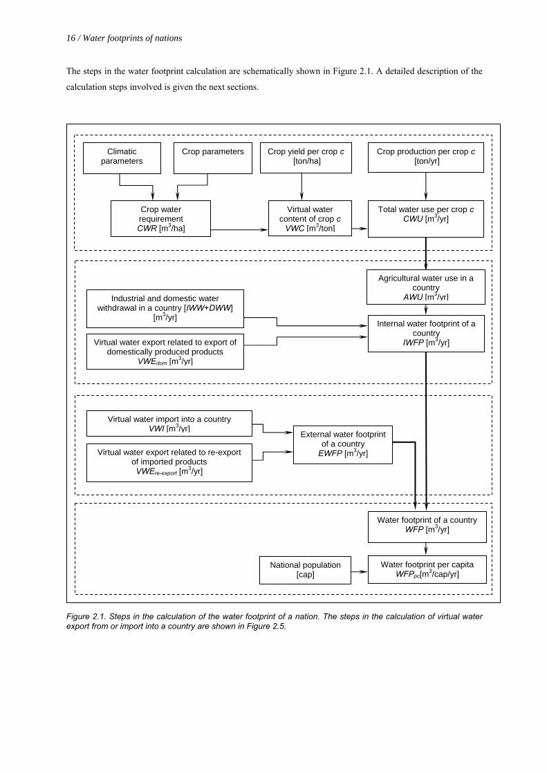
The steps in the water footprint calculation are schematically shown in Figure 2.1. A detailed description of the
calculation steps involved is given the next sections.
Crop production per crop c [ton/yr]
Crop parameters Climatic parameters
Industrial and domestic water withdrawal in a country [IWW+DWW]
[m3/yr]
Crop water requirement CWR [m3/ha]
Total water use per crop c CWU [m3/yr]
Virtual water content of crop c
VWC [m3/ton]
Crop yield per crop c [ton/ha]
Internal water footprint of a country
IWFP [m3/yr]
Figureexport
Virtual water export related to export ofdomestically produced products
VWEdom [m3/yr]
V
2.1 fro
Virtual water import into a countryVWI [m3/yr]
External water footpof a country
EWFP [m3/yr]
National population [cap]
irtual water export related to re-export of imported products VWEre-export [m3/yr]
. Steps in the calculation of the water footprint of a nation. The steps in tm or import into a country are shown in Figure 2.5.
Agricultural water use in a country
AWU [m3/yr]
Water footprint of a country WFP [m3/yr]
Water footprint per capita WFPpc[m3/cap/yr]
rint
he calculation of virtual water

Water footprints of nations / 17
2.2. Use of domestic water resources
2.2.1. Water use for crop production
The total volume of water use to produce crops in a country (AWU, m3/yr), is calculated as:
∑=
=n
cCWUAWUc
c 1][ (5)
where CWU (m3/yr), crop water use, is the total volume of water used in order to produce a particular crop.
][][][][
cYieldcProductioncCWRcCWU ×= (6)
Here, CWR is the crop water requirement measured at field level (m3/ha), Production the total volume of crop c
produced (ton/yr) and Yield the production volume of crop c per unit area of production (ton/ha).
‘Crop water requirement’ is defined as the total water needed for evapotranspiration, from planting to harvest for
a given crop in a specific climate regime, when adequate soil water is maintained by rainfall and/or irrigation so
that it does not limit plant growth and crop yield (Allen et al., 1998). Under standard conditions when a crop
grows without any shortage of water, the crop evapotranspiration is equal to the CWR of a crop. By taking crop
water requirements as an indicator of actual crop water use, we implicitly assume that the crop water
requirements are fully met. This leads to an overestimation of actual crop water use. On the other hand,
however, we underestimate the water needs to grow crops by excluding irrigation losses and drainage
requirements from our analysis. In order to reduce the error made when taking crop water use a function of crop
water requirement, countries where crop yields are very low due to water constraints have been left out from the
analysis.
The crop water requirement is calculated by accumulation of data on daily crop evapotranspiration ETc
(mm/day) over the complete growing period.
∑=
×=lp
dc dcETcCWR
1
],[10][ (7)
Where the factor 10 is meant to convert mm into m3/ha and where the summation is done over the period from
day 1 to the final day at the end of the growing period (lp stands for length of growing period in days). The crop
water requirement of rice cannot be calculated directly using Equation 7. In addition to evapotranspiration from
the paddy field, there is a considerable amount of percolation from the field, which varies with the soil type and
ground water table at the farm. Assuming that rice is normally grown in a loam and loamy clay, we have added
300 mm of water for percolation during plantation period.
s 18 / Water footprints of nation
The crop evapotranspiration per day follows from multiplying the reference crop evapotranspiration ET0 with
the crop coefficient Kc:
0][][ ETcKcET cc ×= (8)
The reference crop evapotranspiration is the evapotranspiration rate from a reference surface, not short of water.
The reference is a hypothetical surface with extensive green grass cover with specific characteristics. The only
factors affecting ETo are climatic parameters. ETo expresses the evaporating power of the atmosphere at a
specific location and time of the year and does not consider the crop characteristics and soil factors. The actual
crop evapotranspiration differs distinctly from the reference evapotranspiration, as the ground cover, canopy
properties and aerodynamic resistance of the crop are different from grass. The effects of characteristics that
distinguish field crops from grass are integrated into the crop coefficient (Kc).
The major factors determining Kc are crop variety, climate and crop growth stage. For instance, more arid
climates and conditions of greater wind speed will have higher values for Kc. More humid climates and
conditions of lower wind speed will have lower values for Kc.
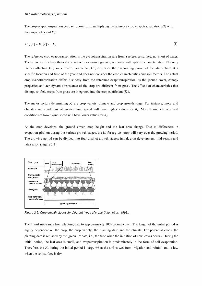
As the crop develops, the ground cover, crop height and the leaf area change. Due to differences in
evapotranspiration during the various growth stages, the Kc for a given crop will vary over the growing period.
The growing period can be divided into four distinct growth stages: initial, crop development, mid-season and
late season (Figure 2.2).
Figure 2.2. Crop growth stages for different types of crops (Allen et al., 1998).
The initial stage runs from planting date to approximately 10% ground cover. The length of the initial period is
highly dependent on the crop, the crop variety, the planting date and the climate. For perennial crops, the
planting date is replaced by the 'green up' date, i.e., the time when the initiation of new leaves occurs. During the
initial period, the leaf area is small, and evapotranspiration is predominately in the form of soil evaporation.
Therefore, the Kc during the initial period is large when the soil is wet from irrigation and rainfall and is low
when the soil surface is dry.
Water footprints of nations / 19
The crop development stage runs from 10% ground cover to effective full cover, which for many crops occurs at
the initiation of flowering. As the crop develops and shades more and more of the ground, evaporation becomes
more restricted and transpiration gradually becomes the major process. During the crop development stage, the
Kc value corresponds to the extent of ground cover. Typically, if the soil surface is dry, Kc = 0.5 corresponds to
about 25-40% of the ground surface covered by vegetation. A Kc value of 0.7 often corresponds to about 40-60%
ground cover. These values will vary, depending on the crop, frequency of wetting and whether the crop uses
more water than the reference crop at full ground cover.
The mid-season stage runs from effective full cover to the start of maturity. The start of maturity is often
indicated by the beginning of the ageing, yellowing or senescence of leaves, leaf drop, or the browning of fruit
to the degree that the crop evapotranspiration is reduced relative to the reference ETo. The mid-season stage is
the longest stage for perennials and for many annuals, but it may be relatively short for vegetable crops that are
harvested fresh for their green vegetation. In the mid-season stage Kc has its maximum value and remains
constant. Deviation of Kc from the reference value '1' is primarily due to differences in crop height and resistance
between the grass reference surface and the actual crop surface.
The late season stage runs from the start of maturity to harvest or full senescence. The calculation of crop
evapotranspiration is presumed to end when the crop is harvested, dries out naturally, reaches full senescence, or
experiences leaf drop. For some perennial vegetation in frost-free climates, crops may grow year round so that
the date of termination may be taken the same as the date of 'planting'. The Kc value at the end of the late season
stage reflects crop and water management practices. The Kc value is high if the crop is frequently irrigated until
harvested fresh. If the crop is allowed to senesce and to dry out in the field before harvest, the Kc value will be
small.
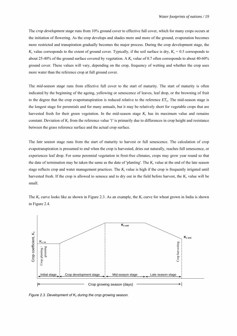
The Kc curve looks like as shown in Figure 2.3. As an example, the Kc curve for wheat grown in India is shown
in Figure 2.4.
Kc end
Kc ini
Cro
p pl
antin
g /
gree
ning
Kc mid
Cro
p ha
rves
ting
Cro
p co
effic
ient
, Kc
Initial stage Crop development stage Mid-season stage Late season stage
Crop growing season (days)
Figure 2.3. Development of Kc during the crop growing season.

s 20 / Water footprints of nation
0.0
1.0
2.0
3.0
4.0
5.0
6.0
01-J
an
21-J
an
10-F
eb
02-M
ar
22-M
ar
11-A
pr
01-M
ay
21-M
ay
10-J
un
30-J
un
20-J
ul
09-A
ug
29-A
ug
18-S
ep
08-O
ct
28-O
ct
17-N
ov
07-D
ec
27-D
ec
Evap
otra
nspi
ratio
n (m
m/d
ay)
0.00
0.50
1.00
1.50
2.00
2.50
3.00
Cro
p co
effic
ient
(Kc)
Total annual crop evapotranspiration ( Wheat, India) = 438 mm/yr
Kc
ETo
ETc
Cro
p pl
antin
g
Cro
p ha
rves
ting
Figure 2.4. Calculation of ETc for wheat grown in India. It also shows the daily distribution of ET0 (mm/day) for India and Kc for wheat planted on 15th of December in India.
Reference crop evapotranspiration
The FAO Penman-Monteith method is used to estimate the reference evapotranspiration ET0. Below we
summarize the method from FAO (Allen et al., 1998),
summarize the method from FAO (Allen et al., 1998),
)34.01(
)(273
900)(408.0
2
2
0 U
eeUT
GRET
asn
++∆
−+
+−∆=
γ
γ (9)
Where
ET0 = reference crop evapotranspiration [mm/day],
∆ = slope of the vapour pressure curve [kPa/°C] (Equation 10),
T = average air temperature [°C] (Equation 11),
γ = psychrometric constant [kPa/°C] (Equation 12),
es = saturation vapour pressure [kPa] (Equation 14),
Rn = net radiation at the crop surface [MJ/m2/day] (Equation 16),
G = soil heat flux [MJ/m2/day] (Equation 26),
U2 = wind speed measured at 2 m height [m/s],
ea = actual vapour pressure [kPa],
es-ea = vapour pressure deficit [kPa].
Equation 9 is applied with a time step of a month. For all input data, monthly averages have been taken. A
smooth graph of ET0 over the year has been obtained by assuming that the calculated monthly averages hold for
the 15th of the month and by assuming linear development in between the 15th of one month and 15th of next
month. The various parameters in Equation 9 are calculated in different steps.
Water footprints of nations / 21
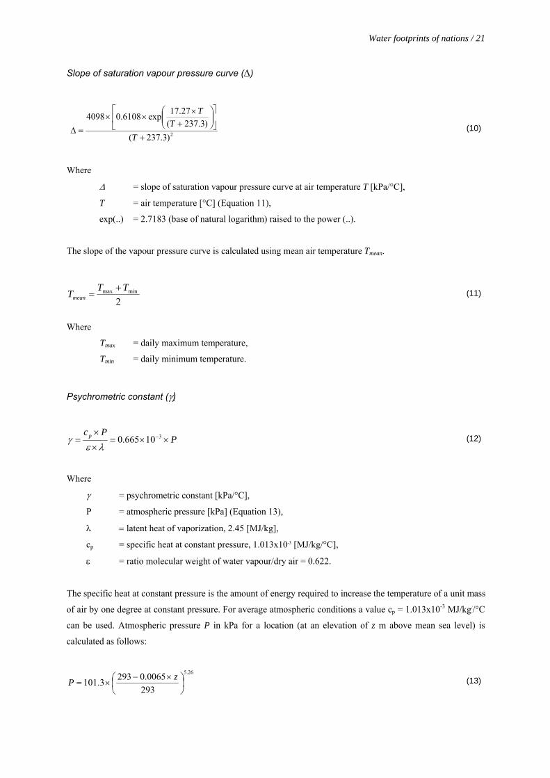
Slope of saturation vapour pressure curve (∆)
2)3.237(
)3.237(27.17exp6108.04098
+
⎥⎦
⎤⎢⎣
⎡⎟⎟⎠
⎞⎜⎜⎝
⎛+
×××
=∆T
TT
(10)
Where
∆ = slope of saturation vapour pressure curve at air temperature T [kPa/°C],
T = air temperature [°C] (Equation 11),
exp(..) = 2.7183 (base of natural logarithm) raised to the power (..).
The slope of the vapour pressure curve is calculated using mean air temperature Tmean.
2minmax TTTmean
+= (11)
Where
Tmax = daily maximum temperature,
Tmin = daily minimum temperature.
Psychrometric constant (γ)
PPcp ××=
×
×= −310665.0
λεγ (12)
Where
γ = psychrometric constant [kPa/°C],
P = atmospheric pressure [kPa] (Equation 13),
λ = latent heat of vaporization, 2.45 [MJ/kg],
cp = specific heat at constant pressure, 1.013x10⁻³ [MJ/kg/°C],
ε = ratio molecular weight of water vapour/dry air = 0.622.
The specific heat at constant pressure is the amount of energy required to increase the temperature of a unit mass
of air by one degree at constant pressure. For average atmospheric conditions a value cp = 1.013x10⁻³ MJ/kg//°C
can be used. Atmospheric pressure P in kPa for a location (at an elevation of z m above mean sea level) is
calculated as follows:
26.5
2930065.02933.101 ⎟
⎠⎞
⎜⎝⎛ ×−
×=zP (13)
s 22 / Water footprints of nation
Mean saturation vapour pressure (es)
2min)(
0max)(
0TT
seee +
= (14)
Where e0(Tmax) and e0
(Tmin) are calculated as follows:
⎟⎟⎠
⎞⎜⎜⎝
⎛+
××=
)3.237(27.17exp6108.0)(
0
TTe T (15)
Net radiation (Rn) The net radiation is the difference between the incoming net shortwave radiation (Rns) and the outgoing net
longwave radiation (Rnl):
nlnsn RRR −= (16)
The net shortwave radiation (Rns,) resulting from the balance between incoming and reflected solar radiation is
given by:
( ) sns RR ×−= α1 (17)
Where
Rns = net solar or shortwave radiation [MJ/m2/day],
α = albedo or canopy reflection coefficient, which is 0.23 for the hypothetical grass reference crop,
Rs = the incoming solar radiation [MJ/m2/day] (Equation 19).
Net longwave radiation (Rnl) is given by the Stefan-Boltzmann equation.
( ) ( ) ( ) ⎟⎟⎠
⎞⎜⎜⎝
⎛−××−×⎥
⎦
⎤⎢⎣
⎡ +×= 35.035.114.034.0
2 0
min,4
max,4
s
sa
KKnl R
ReTTR σ (18)
Where
Rnl = net outgoing longwave radiation [MJ/m2/day],
σ = Stefan-Boltzmann constant [4.903 x 10⁻⁹ MJ/K4/m2/day],
Tmax, K = maximum absolute temperature during the 24-hour period [K = °C + 273.16],
Tmin, K = minimum absolute temperature during the 24-hour period [K = °C + 273.16],
ea = actual vapour pressure [kPa],
Rs/Rso = relative shortwave radiation (limited to ≤ 1.0),
Rs = solar radiation [MJ/m2/day] (Equation 19),
Rso = clear-sky radiation [MJ/m2/day] (Equation 20).

Water footprints of nations / 23
Solar radiation (Rs) can be calculated with the Angstrom formula, which relates solar radiation to extraterrestrial
radiation and relative sunshine duration:
asss RNnbaR ×⎟
⎠⎞
⎜⎝⎛ ×+= (19)
Where
Rs = solar or shortwave radiation [MJ/m2/day],
n = actual duration of sunshine [hour],
N = maximum possible duration of sunshine or daylight hours [hour],
n/N = relative sunshine duration = (1-Percentage cloud cover expressed in fraction) [dimensionless],
Ra = extraterrestrial radiation [MJ/m2/day] (Equation 21),
as = regression constant, expressing the fraction of extraterrestrial radiation reaching the earth on
overcast days (n = 0),
as+bs = fraction of extraterrestrial radiation reaching the earth on clear days (when n = N).
Depending on atmospheric conditions (humidity, dust) and solar declination (latitude and month), the Angstrom
values as and bs will vary. Where no actual solar radiation data are available and no calibration has been carried
out for improved as and bs parameters, the values as = 0.25 and bs = 0.50 are taken as recommended by Allen et
al. (1998).
The clear-sky radiation, Rso, when n = N, is calculated as:
( ) as RzR ×××+= −60 10275.0 (20)
Where, Ra is extraterrestrial radiation (MJ/m2/day, Equation 21) and z is the elevation above mean sea level (m).
The extraterrestrial radiation, Ra, for each day of the year and for different latitudes can be estimated from the
solar constant, the solar declination and the time of the year.
( ) [ ])sin()cos()cos()sin()sin(6024ssrsca dGR ωδϕδϕω
π+×
×= (21)
Where
Ra = extraterrestrial radiation [MJ/m2/day],
Gsc = solar constant = 0.0820 [MJ/m2/day],
dr = inverse relative distance Earth-Sun (Equation 22),
ω s = sunset hour angle [rad] (Equation 25),
ϕ = latitude [rad] (Equation 24),
δ = solar decimation [rad] (Equation 23).
s 24 / Water footprints of nation
The inverse relative distance Earth-Sun, dr, and the solar declination, δ, are given by:
⎟⎠⎞
⎜⎝⎛×+= Jd r 365
2cos033.01 π (22)
⎟⎠⎞
⎜⎝⎛ −×= 39.1
3652sin409.0 Jπδ (23)
Where J is the number of the day in the year between 1 (1 January) and 365 or 366 (31 December). The latitude,
ϕ, expressed in radians is positive for the northern hemisphere and negative for the southern hemisphere.
[ ] [ ]degrees decimal180
radians πϕ = (24)
The sunset hour angle, ωs, is given by:
)]tan()tan(arccos[ δϕω −=s (25)
Soil heat flux (G) Complex models are available to describe soil heat flux. Because soil heat flux is small compared to Rn,
particularly when the surface is covered by vegetation, for monthly average G, we can use the following:
( )1,1,, 07.0 −+ −×= imonthimonthimonth TTG (26)
Where
Tmonth, i = mean air temperature of month i [°C] (Equation 11),
Tmonth, i-1 = mean air temperature of previous month [°C] (Equation 11),
Tmonth, i+1 = mean air temperature of next month [°C] (Equation 11).
2.2.2. Water use in the industrial and domestic sectors
For data on water use in the industrial and domestic sectors we use available statistics. The industrial water
withdrawal includes process water required in different stages of production. Domestic water withdrawal
incorporates the blue water withdrawn to meet the per capita demand for household and municipal consumption.

Water footprints of nations / 25
2.3. The export of domestic water resources and the import of foreign water resources
2.3.1. Virtual water content of primary crops
The virtual water content of a crop c in a country (m3/ton) is calculated as the ratio of total water used for the
production of crop c to the total volume of crop produced in that country.
][][][
cProductioncCWUcVWC = (27)
where CWU [c] is the volume of water use at farm level for the production of crop c in the country (m3/yr) and
Production [c] the total volume of crop c produced per year in the country (ton/yr).
2.3.2. Virtual water content of live animals
The virtual water content of an animal at the end of its life span is defined as the total volume of water that was
used to grow and process its feed, to provide its drinking water, and to clean its housing and the like. It depends
on the breed of an animal, the farming system, the feed consumption and the climatic conditions of the place
where the feed is grown.
There are three components to the virtual water content (VWC) of a live animal a:
][][][][ aVWCaVWCaVWCaVWC servdrinkfeed ++= (28)
VWCfeed[a], VWCdrink[a] and VWCserv[a] represent the virtual water content of animal a related to feed, drinking
water and service water consumption respectively, expressed in cubic metres of water per ton of live animal.
The virtual water content of an animal at the end of its life span from the feed consumed has two parts. The first
is the actual water that is required to prepare the feed mix and the second is the virtual water incorporated in the
various feed ingredients.
][
],[][][
][1
aW
dtn
caFeedcVWCaq
aVWC
slaughter
birth cmixing
feed
c
∫ ∑⎪⎭
⎪⎬⎫
⎪⎩
⎪⎨⎧
×+
==
(29)
The variable qmixing [a] represents the volume of water required for mixing the feed (m3/day). Feed[a,c] is the
quantity of feed crop c consumed by the animal, expressed in tons per day. W [a] is the live weight of the animal
at the end of its life span, expressed in tons.
s 26 / Water footprints of nation
The virtual water content of an animal originating from drinking is equal to the total volume of water withdrawn
for drinking water supply, calculated over the entire life span of the animal.
][
][][
aW
dtaqaVWC
slaughter
birthd
drink
∫= (30)
The virtual water content of an animal from the service water used is equal to the total volume of water used to
clean the farmyard, wash the animal and other services necessary to maintain the environment during the entire
life span of the animal.
][
][][
aW
dtaqaVWC
slaughter
birthserv
serv
∫=
(31)
qd[a] and qserv[a] are the daily drinking water requirement and the daily service water requirement of the animal
respectively (m3/day).
2.3.3. Virtual water content of processed crop and livestock products
The virtual water content of a processed product depends on the virtual water content of the primary crop or live
animal from which it is derived. The virtual water content of the primary crop or live animal is distributed over
the different products from that specific crop or animal. We have assumed that each individual crop or livestock
product p comes from one and only one particular type of primary crop c or live animal a. For simplification it
is further assumed that a product p exported from a certain country e is actually produced from a primary crop c
or animal a grown within that country using the domestic resources only.
For the sake of systematic analysis we assume ‘levels of production’. The products derived directly from a
primary crop or a live animal are called primary products. For example, cows produce milk, a carcass and skin
as their primary products. From paddy (rice) we get husked rice as a primary crop product. From soybean we
get soybean crude oil and soybean oil cakes as primary crop products. Some of these primary products are
further processed into so-called secondary products, such as cheese and butter made from the primary product
milk, flour made from husked rice and meat and sausage processed from the carcass.
The virtual water content of a processed product from a primary crop or a live animal includes (part of) the
virtual water content of the primary crop or live animal plus the processing water needed. The processing water
requirement is calculated as follows:

Water footprints of nations / 27
][][
][aorcW
aorcQaorcPWR proc=
(32)
Here PWR[c or a] is the processing water requirement per ton of primary crop c or live animal a for producing
primary products in a country (m3/ton). Qproc[c or a] is the total volume of processing water required (m3) to
process crop c or animal a. W[c or a] is the total weight of the primary crop or live animal processed.
The sum of processing water requirement (PWR) and the virtual water content of the primary crop (VWCc) or the
virtual water content of the live animal (VWCa) should be attributed to the processed products in a logical way.
To do this we introduce the terms product fraction and value fraction. The product fraction pf[p] of product p is
defined as the weight of the primary product obtained per ton of primary crop or live animal (Chapagain and
Hoekstra, 2003a). For example, if one ton of paddy (rice) produces 0.62 ton of husked rice, the product fraction
of husked rice is 0.62. The pf’s for crop and livestock products are calculated respectively as follows:
][][
][cWpW
ppf p= (33a)
][][
][aWpW
ppf p= (33b)
Here Wp[p] is the weight of primary product p obtained from processing W[c] ton of primary crop c or W[a] ton
of live animal a. Generally the product fraction is less than one, because the product is derived from just part of
the animal or crop. However, if a product is obtained during the lifetime of an animal, as in the case of milk and
eggs, the pf can be greater than one (Chapagain and Hoekstra, 2003a).
If there are more than two products obtained while processing a primary crop or a live animal, we need to
distribute the virtual water content of the primary crop or the live animal to its products based on value fractions
and product fractions. The value fraction, vf[p], of a product is the ratio of the market value of the product to the
aggregated market value of all the products obtained from the primary crop or live animal:
( )∑ ×
×=
][][
][][][ppfpv
ppfpvpvf
(34)
The denominator is totalled over the primary products that originate from the primary crop c or the animal a.
The variable v[p] is the market value of product p (US$/ton). Hence, the virtual water content (VWC) of primary
product p in m3/ton is:

s 28 / Water footprints of nation
( )][][]or[]or[][
ppfpvfacPWRacVWCpVWC ×+= (35)
In a similar way we can calculate the virtual water content for secondary and tertiary products, etc. The first step
is always to obtain the virtual water content of the input (root) product and the water necessary to process it. The
total of these two elements is then distributed over the various output products, based on their product fraction
and value fraction. The list of crop products and their product fractions is presented in Appendix X.
For example, 1 ton of soybean produces 0.85 tons of soybean flour. If the virtual water content of soybean is
1789 m3/ton, the virtual water content of soybean flour is 2105 (= 1789/0.85) m3/ton. Instead of processing
soybeans into soybean flour, we can also process soybeans into soybean crude oil (pfsoybean crude oil = 0.18 ton per
ton of soybean) and soybean oil cake (pfsoybean oil cake = 0.79 ton per ton of soybean). The global average market
value of soybean crude oil is 502 US$/ton and soybean oil cake is 219 US$/ton. The total market value of
soybean crude oil is, thus, 90 US$ (= 502*0.18) and the market value of soybean oil cake produced is 173 US$
(=0.79*219). The total market value produced is 263 US$ (= 90+173). Hence, the value fraction of soybean
crude oil is 0.343 (vfsoybean crude oil = 90/263) and for the soybean oil cake it is 0.657 (vfsoybean oil cake = 173/263).
Neglecting process water requirements, the virtual water content of the two products from soybean can be
calculated as:
VWCsoybean * vfsoybean crude oil Virtual water content of soybean crude oil =
pfsoybean crude oil
=
1789 * 0.343
0.18 ≈ 3410 m3/ton
VWCsoybean * vfsoybean oi cake Virtual water content of soybean oil cake =
pfsoybean oil cake
=
1789 * 0.657
0.79 ≈ 1490 m3/ton
2.3.4. Virtual water flows related to the trade in agricultural products
International virtual water flows related to trade in agricultural products are calculated by multiplying the trade
volumes with their respective virtual water content. The virtual water content of a traded crop or livestock
product depends on where and how the product has been produced. We assume here that the products have been
produced in the exporting country.
The virtual water flow VWF (m3/yr) from exporting country e to importing country i as a result of export of an
agricultural product p can be calculated as:

Water footprints of nations / 29
[ ] [ ] [ ] peVWCpiePTpieVWF ,,,,, ×= (36)
Here, PT represents the product trade (ton/yr) from exporting country e to importing country i while VWC is the
virtual water content (m3/ton) of product p in the exporting country.
2.3.5. Virtual water flows related to the trade in industrial products
The virtual water content of an industrial product can be calculated in a similar way as described earlier for
agricultural products. There are however numerous categories of industrial products with a diverse range of
production methods and detailed standardised national statistics related to the production and consumption of
industrial products are hard to find. As the global volume of water withdrawn in the industrial sector is only 716
Gm3/yr (≈ 10% of total global water use), we have – per country – simply calculated an average virtual water
content per dollar added value in the industrial sector (VWC, m3/US$) as:
][][][
eGDPeIWWeVWC
i
= (37)
Here IWW is the industrial water withdrawal (m3/yr) in a country, while GDPi is the added value of the industrial
sector, which is one component of the national GDP (US$/yr).
The global average virtual water content of industrial products (VWCg) is defined as:
[ ]
∑
∑
=
== n
ei
n
eg
eGDP
eIWWVWC
1
1
][
(38)
The total volume of virtual water exported from country e as a result of export of industrial products (VWE) is
obtained by multiplying the export value of industrial products by the virtual water content per dollar (VWC).
[ ] ][][ eproductsindustrialofvalueExporteVWCeVWE ×= (39)
The virtual water import related to the import of industrial products (VWI) is calculated using the global average
virtual water content in the industrial sector (VWCg).
[ ] ][eproductsindustrialofvalueImportVWCeVWI g ×= (40)

30 / Water footprints of nations
2.3.6. Virtual water balance of a country
The difference between total virtual water import and total virtual water export is the virtual water flow balance
of the country in the time period concerned. If the balance is positive it implies net virtual water being imported
and if it is negative there is net export of virtual water.
The various steps in the calculation of virtual water flows leaving and entering a country are presented
schematically in Figure 2.5.

Water footprints of nations / 31
Figure 2.5. Steps in the calculation of virtual water flowindustrial products.
Production fraction pf and
Value fraction vf
Crop parameters
Climatic parameters
Trade in crop and livestock products
[ton/yr]
Crop water requirement CWR [m3/ha]
Feed volume per feed crop [ton/animal]
Drinking and servicing water requirement
[ton/animal]
Virtual water content of primary crop c VWC [m3/ton]
Crop yield per crop c [ton/ha]
s re
late
d to
trad
e in
e
prod
ucts
ltu
ral [
m3 /y
r]
Virtual water content of crop products VWC [m3/ton]
Process water requirement PWR[m3/ton]
Production fraction pf and
value fraction vf
Value added from industrial sector GDPi [US$/yr]
Industrial water withdrawal
IWW [m3/yr]
Virtual waind
Global-avcontent of
VW
Value of exported industrial products
[US$/yr]
Country-acontent of
VW
Virtual water content of liveanimal a [m3/ton]
s
Virt
ual w
ater
flow
agric
ultu
rV
WF a
gric
u
teuV
er inC
ve inC
Virtual water content oflivestock products
[m3/ton]
age virtual water dustrial products
g [m3/US$]
rage virtual water dustrial products [m3/US$]
r flo
ws
rela
ted
to th
e in
tern
atio
nal
trade
of p
rodu
cts
VW
F ind
ustri
al [m
3 /yr]
Value of imported industrial products
[US$/yr]
Virtual water import with import of industrial products
VWI [m3/yr]
Process water requirementPWR [m3/ton]
of a country related to international trade of agricultural and
r export with export of strial products WE [m3/yr] V
irtua
l wat
e
s 32 / Water footprints of nation
2.4. Water scarcity, water self-sufficiency and water import dependency of a nation
We define water scarcity (WS) of a nation as the ratio of the nation’s water footprint (WFP) to the nation’s water
availability (WA).
100×=WA
WFPWS (41)
The national water scarcity can be more than 100% if there is more water needed for producing the foods and
services consumed by the people of a nation than is available in the country. As a measure of water availability
we take here the ‘total renewable water resources (actual)’ as defined by FAO in their AQUASTAT database.
We define water import dependency (WD, %) of a nation as the ratio of the external water footprint (EWFP,
m3/yr) to the total water footprint (WFP, m3/yr) of a country.
100×=WFPEWFPWD (42)
National water self-sufficiency (WSS, %) is defined as the internal water footprint (IWFP, m3/yr) divided by the
total water footprint.
100×=WFPIWFPWSS (43)
Self-sufficiency is 100% if all the water needed is available and indeed taken from within the own territory.
Water self-sufficiency approaches zero if the demands of goods and services in a country are heavily met with
gross virtual water imports, i.e. it has relatively large external water footprint in comparison to its internal water
footprint.
Water footprints of nations / 33
3. Scope and data
3.1. Country coverage
For the calculation of reference evapotranspiration, crop water requirement and consequently virtual water
content of different primary crops we have taken 210 countries (see Appendix II) for which the production and
yield data are available in the on-line database of FAO (FAOSTAT, 2004).
For the calculation of international virtual water flows, that determine the external water footprints, we have
taken into account the trade between 243 countries and territories for which international trade data are available
in the Personal Computer Trade Analysis System (PC-TAS, 2004) of the International Trade Centre,
UNCTAD/WTO. It covers trade data from 146 reporting countries and territories disaggregated by product and
partner countries (UNSD, 2004a). The list of reporting and partner countries and territories as available in PC-
TAS (2004) is presented in Appendix II.
For the 97 countries and territories that are not reporting country but are included as partner country
nevertheless, the export and import data are estimated using mirror statistic from the trade data of the reporting
countries. For example, if we want to estimate Viet Nam’s exports to Indonesia, we look at what Indonesia
reports about its imports from Viet Nam. This role reversal is used in cases where the concerned country has not
been providing up-to-date information on its trade flow. It can also help as a means to double-check the
reporter’s information. The international trade flows between non-reporting countries are not covered in this
study.
3.2. Product coverage
The total water footprint is calculated as the sum of the use of domestic water resources and virtual water import
minus virtual water export. The use of domestic water resources is the sum of three components: volume of
industrial water withdrawal, volume of domestic water withdrawal and crop evapotranspiration. Data on
domestic water withdrawals have been taken from AQUASTAT (FAO, 2003f, g). We have assumed that the
domestic water withdrawal is equal to the consumption. The study covers all the industrial products through a
relatively simple approach. Per country, we simply consider total industrial water withdrawal as reported in
AQUASTAT (FAO, 2003f, g). The volume of water used for crop production (crop evapotranspiration) in a
country is estimated using the production data per country covering 164 types of primary crops (as defined in
FAOSTAT, 2004). The list of primary crops and their product codes in FAOSTAT is presented in Appendix III.
The volume of virtual water export or import is calculated based on the international trade of products and their
virtual water content. As for trade in agricultural products, we have taken trade data from PC-TAS (2004). The
28 relevant product groups in PC-TAS are presented in Table 3.1. We have calculated the virtual water content
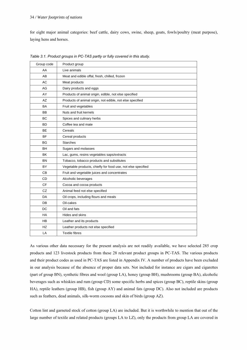
34 / Water footprints of nationso
for eight major animal categories: beef cattle, dairy cows, swine, sheep, goats, fowls/poultry (meat purpose),
laying hens and horses.
Table 3.1. Product groups in PC-TAS partly or fully covered in this study.
Group code Product group
AA Live animals
AB Meat and edible offal, fresh, chilled, frozen
AC Meat products
AG Dairy products and eggs
AY Products of animal origin, edible, not else specified
AZ Products of animal origin, not edible, not else specified
BA Fruit and vegetables
BB Nuts and fruit kernels
BC Spices and culinary herbs
BD Coffee tea and mate
BE Cereals
BF Cereal products
BG Starches
BH Sugars and molasses
BK Lac, gums, resins vegetables saps/extracts
BN Tobacco, tobacco products and substitutes
BY Vegetable products, chiefly for food use, not else specified
CB Fruit and vegetable juices and concentrates
CD Alcoholic beverages
CF Cocoa and cocoa products
CZ Animal feed not else specified
DA Oil crops, including flours and meals
DB Oil-cakes
DC Oil and fats
HA Hides and skins
HB Leather and its products
HZ Leather products not else specified
LA Textile fibres
As various other data necessary for the present analysis are not readily available, we have selected 285 crop
products and 123 livestock products from these 28 relevant product groups in PC-TAS. The various products
and their product codes as used in PC-TAS are listed in Appendix IV. A number of products have been excluded
in our analysis because of the absence of proper data sets. Not included for instance are cigars and cigarettes
(part of group BN), synthetic fibres and wool (group LA), honey (group BH), mushrooms (group BA), alcoholic
beverages such as whiskies and rum (group CD) some specific herbs and spices (group BC), reptile skins (group
HA), reptile leathers (group HB), fish (group AY) and animal fats (group DC). Also not included are products
such as feathers, dead animals, silk-worm cocoons and skin of birds (group AZ).
Cotton lint and garneted stock of cotton (group LA) are included. But it is worthwhile to mention that out of the
large number of textile and related products (groups LA to LZ), only the products from group LA are covered in

Water footprints of nations / 35
the present study. Textile products in the groups fibre waste (LB), textile yarns and threads (LC), textile fabrics
(LD) etc. include products derived from different primary products such as cotton, artificial fibres, wool or a mix
of different materials. These products are quite diverse in nature and are made up of from crop and artificial
fibres which are not categorically specified in the trade database.
As for trade in industrial products, we have taken trade data from the World Trade Organisation (WTO, 2004a,
b). Virtual water imports and exports are calculated by multiplying monetary data on international trade of
industrial products by country specific data on the average virtual water content per dollar of industrial products.
In this approach, all industrial products are included implicitly.
3.3. Input data
3.3.1. Population, land and water resources
Data on population per country have been taken from the World Bank online database (World Bank, 2004).
Wherever the population data are not available in this database, data have been taken from FAO (FAOSTAT,
2004). The available data have been averaged for the period 1997-2001. Arable land is taken from FAO
(FAOSTAT, 2004) for the period 1997-2001. Data on total renewable water resources and water withdrawals
per country have also been taken from FAO (FAO, 2003f, g). The input data used have been summarised in
Appendix V.
3.3.2. Gross national income, gross domestic production and added value in the industrial sector
The average gross national income (GNI in US$/yr) for the period 1998-2001 have been taken from the World
Bank on-line database (World Bank, 2004). The gross domestic products are taken from the UNSD for current
US$ (UNSD, 2004b) for the period of 1997-2001. Data for the countries missing in the list of UNSD are taken
from IMF (2004).
Data on the contribution of the industrial sector to the gross domestic product have been taken from the on-line
data source of the World Bank (2004). There are still some countries missing in the database. For these
countries, the percentage share of industrial sector to the national GDP has been taken from the on-line data
source of Frederick S. Pardee Centre (2004) and CIA (2004).
3.3.3. International trade data
Data on international trade in agricultural products have been taken from the Personal Computer Trade Analysis
System (PC-TAS, 2004) of the International Trade Centre. Data on international trade in industrial products
have been taken from the World Trade Organisation (WTO, 2004a,b).

36 / Water footprints of nationso
The export data do not categorically specify whether they refer to the export of goods that are produced
domestically or the re-export of imported products. The virtual water export VWE (m3/yr) from a country is
however made up of two components: virtual water export related to the export of domestic products (VWEdom)
and virtual water export related to the re-export of imported from other countries (VWEre-export).
ortredom VWEVWEVWE exp−+= (44)
We have assumed that the two components can be estimated based on the relative share of the use of domestic
water resources and the virtual water import respectively.
VWIDWWIWWAWU
DWWIWWAWUVWEVWEdom +++++
×=
(45)
VWIDWWIWWAWUVWIVWEVWE ortre +++
×=−exp
(46)
3.3.4. Climate data
The country average data for actual vapour pressure (ea), daily maximum temperature (Tmax), daily minimum
temperature (Tmin) and percentage cloud cover (1-n/N) for each country are taken from the on-line database of
the Tyndall Centre for Climate Change and Research (Mitchell, 2003). The data available here are averages over
the recent past (1961-90) for nine climate variables. The latitude (ϕ) and the average elevation (z) are taken for
the capital of each country.
The data for wind speed (U2) are taken from the database CLIMWAT (FAO, 2003b) for 140 countries and
territories (Appendix II). For many countries climatic data are available for a number of climate stations. In this
study we have taken the wind speed data for the climate station at or nearby the capital of the country. For
countries where wind speed data were absent at all, we have taken data from the neighbouring country with
similar climate. In some remaining cases we have adopted an average wind speed of 2 m/s as recommended by
Allen et al. (1998).
3.3.5. Crop parameters
Countries in different climatic regions generally grow different crop varieties, which often have different crop
parameters. The planting date also varies from country to country. The selection of crop type and suitable
growing period for a particular type of crop in a country largely depends upon the climate of the country and
many other factors like local customs, traditions, social structure, existing norms and policies. Here we have
broadly assumed that the current practices adopted by the farmers are already best alternatives and the crops
grown in similar climatic regions share similar crop parameters.

Water footprints of nations / 37
We have grouped countries into 10 different groups based on their climatic character. The different climates and
their characteristics are presented in Table 3.2. This classification is based on the definition of different thermal
climatic regions given by FAO (2003c).
Table 3.2. Criteria for thermal climate classification.
Climate region Criteria1
Tropics − All months with monthly mean temperatures, corrected to sea level, above 18° C.
Subtropics summer rainfall
− One or more months with monthly mean temperatures, corrected to sea level, below 18 °C but above 5 °C.
− Northern hemisphere: rainfall in April-September rainfall in October-March.
− Southern hemisphere: rainfall in October-March rainfall in April-September.
Subtropics winter rainfall
− One or more months with monthly mean temperatures, corrected to sea level, below 18 °C but above 5 °C.
− Northern hemisphere: rainfall in October-March rainfall in April-September.
− Southern hemisphere: rainfall in April-September rainfall in October-March.
Oceanic temperate − At least one month with monthly mean temperatures, corrected to sea level, below 5°
C and four or more months above 10° C. − Seasonality2 less than 20° C.
Sub-continental temperate − At least one month with monthly mean temperatures, corrected to sea level, below 5°
C and four or more months above 10° C. − Seasonality2 20-35° C.
Continental temperate − At least one month with monthly mean temperatures, corrected to sea level, below 5°
C and four or more months above 10° C. − Seasonality2 more than 35° C.
Oceanic boreal − At least one month with monthly mean temperatures, corrected to sea level, below 5°
C and more than one but less than four months above 10° C. − Seasonality2 less than 20° C.
Sub-continental boreal − At least one month with monthly mean temperatures, corrected to sea level, below 5°
C and more than one but less than four months above 10° C. − Seasonality2 20-35° C.
Continental boreal − At least one month with monthly mean temperatures, corrected to sea level, below 5°
C and more than one but less than four months above 10° C. − Seasonality2 more than 35° C.
Polar/Artic − All months with monthly mean temperatures, corrected to sea level, below 10° C. 1 Source: FAO (2003c) 2 Seasonality refers to the difference in mean temperature of the warmest and coldest month.
Crop coefficients Kc for different crops are taken from FAO (Table 12 in Allen et al., 1998). Whenever data for
different crop parameters are not available for a particular crop type, the crops are first sorted out into different
crop groups as defined by Allen et al. (1998) such as legumes, small vegetables, tropical tree and others. Then
group average values of crop parameters for these crops are taken. The planting dates and cropping calendar are
chosen based on the best available data. Crop calendars for some important crops are available for 90 countries
in a study made by FAO (2003e). Data for crop lengths of different crops grown in different parts of the globe
are available in FAO (Table 11 in Allen et al., 1998). The crop parameters per primary crop per climatic region
are tabulated in Appendix VI.
38 / Water footprints of nationso
3.3.6. Crop production volumes and crop yields
Data on average crop yield per primary crop (ton/ha) per country during 1997-2001 are taken from the on-line
database of FAO (FAOSTAT, 2004) (Appendix VII). If crop yield is not available for that period we have used
the global average crop yield for the concerned crop for the same period. The annual production data (ton/yr) for
164 primary crops are also taken from FAOSTAT (2004) for the period 1997-2001 and are presented in
Appendix VIII.
3.3.7. Product fractions and value fractions of crop and livestock products
Crop and livestock products have been arranged in product trees, some of which are presented in Appendix IX.
For each product, we have assumed a constant set of product fractions pf and value fractions vf across the globe.
The product fractions for various crop and livestock products are derived from different commodity trees as
defined in FAO (2003h) and production data from other sources. Based on the average world market price
(Appendix IV) the value fraction vf for each product is calculated using Equation 34 and the results are
presented in Appendix X. The virtual water content of a product is directly proportional to its vf and inversely
proportional to its pf.
3.3.8. Process water requirements
The volume of process water requirement depends upon the type of product processed and the technology
involved. For any specific product the processing water requirement is more or less the same across different
countries. There are minor variations, based on the efficiency of water use depending on recycling percentage,
cooling processes, etc. As the processing water is only a small part of the virtual water content of a crop or a
livestock product, it will not affect the end results of the study if we assume one constant value for a specific
product across the globe. The data for processing of livestock products are taken from Chapagain and Hoekstra
(2003a). For crop products we have assumed that the processing water requirement is relatively small compared
to the virtual water content of the primary crop and we have neglected these values in the subsequent calculation
of the virtual water content of the processed crop products.

Water footprints of nations / 39
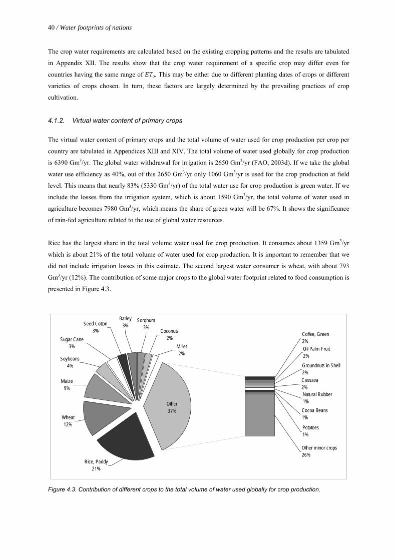
4. Water footprints
4.1. Water needs by product
4.1.1. Reference evapotranspiration and crop water requirement
The monthly average reference evapotranspiration ET0 (mm/day) per country has been calculated as presented in
Appendix XI. ET0 is a climatic parameter expressing the evaporative power of the atmosphere. As we have taken
country average climatic data for the calculation of ET0 we see abrupt changes at the borders of different
countries (Figure 4.1 and 4.2). It is clear that the countries near the tropics have in general higher reference
evapotranspiration rates around the year. As a consequence of this climatic effect, the crop water requirements
of crops grown in these areas are also generally high.
ETo (mm/day)0 - 11 - 22 - 33 - 44 - 55 - 66 - 77 - 12No Data
Figure 4.1. Monthly average reference evapotranspiration per country (mm/day) in June.
ETo (mm/day)0 - 11 - 22 - 33 - 44 - 55 - 66 - 77 - 12No Data
Figure 4.2. Monthly average reference evapotranspiration per country (mm/day) in December.
40 / Water footprints of nationso
The crop water requirements are calculated based on the existing cropping patterns and the results are tabulated
in Appendix XII. The results show that the crop water requirement of a specific crop may differ even for
countries having the same range of ETo. This may be either due to different planting dates of crops or different
varieties of crops chosen. In turn, these factors are largely determined by the prevailing practices of crop
cultivation.
4.1.2. Virtual water content of primary crops
The virtual water content of primary crops and the total volume of water used for crop production per crop per
country are tabulated in Appendices XIII and XIV. The total volume of water used globally for crop production
is 6390 Gm3/yr. The global water withdrawal for irrigation is 2650 Gm3/yr (FAO, 2003d). If we take the global
water use efficiency as 40%, out of this 2650 Gm3/yr only 1060 Gm3/yr is used for the crop production at field
level. This means that nearly 83% (5330 Gm3/yr) of the total water use for crop production is green water. If we
include the losses from the irrigation system, which is about 1590 Gm3/yr, the total volume of water used in
agriculture becomes 7980 Gm3/yr, which means the share of green water will be 67%. It shows the significance
of rain-fed agriculture related to the use of global water resources.
Rice has the largest share in the total volume water used for crop production. It consumes about 1359 Gm3/yr
which is about 21% of the total volume of water used for crop production. It is important to remember that we
did not include irrigation losses in this estimate. The second largest water consumer is wheat, with about 793
Gm3/yr (12%). The contribution of some major crops to the global water footprint related to food consumption is
presented in Figure 4.3.
Cassava2%Natural Rubber1%
Oil Palm Fruit2%
Groundnuts in Shell2%
Rice, Paddy21%
Other37%
Other minor crops26%
Potatoes1%
Cocoa Beans1%Wheat
12%
Maize9%
Soybeans4%
Sugar Cane3%
Seed Cotton3%
Barley3%
Sorghum3%
Coconuts2%
Millet2%
Coffee, Green2%
Figure 4.3. Contribution of different crops to the total volume of water used globally for crop production.
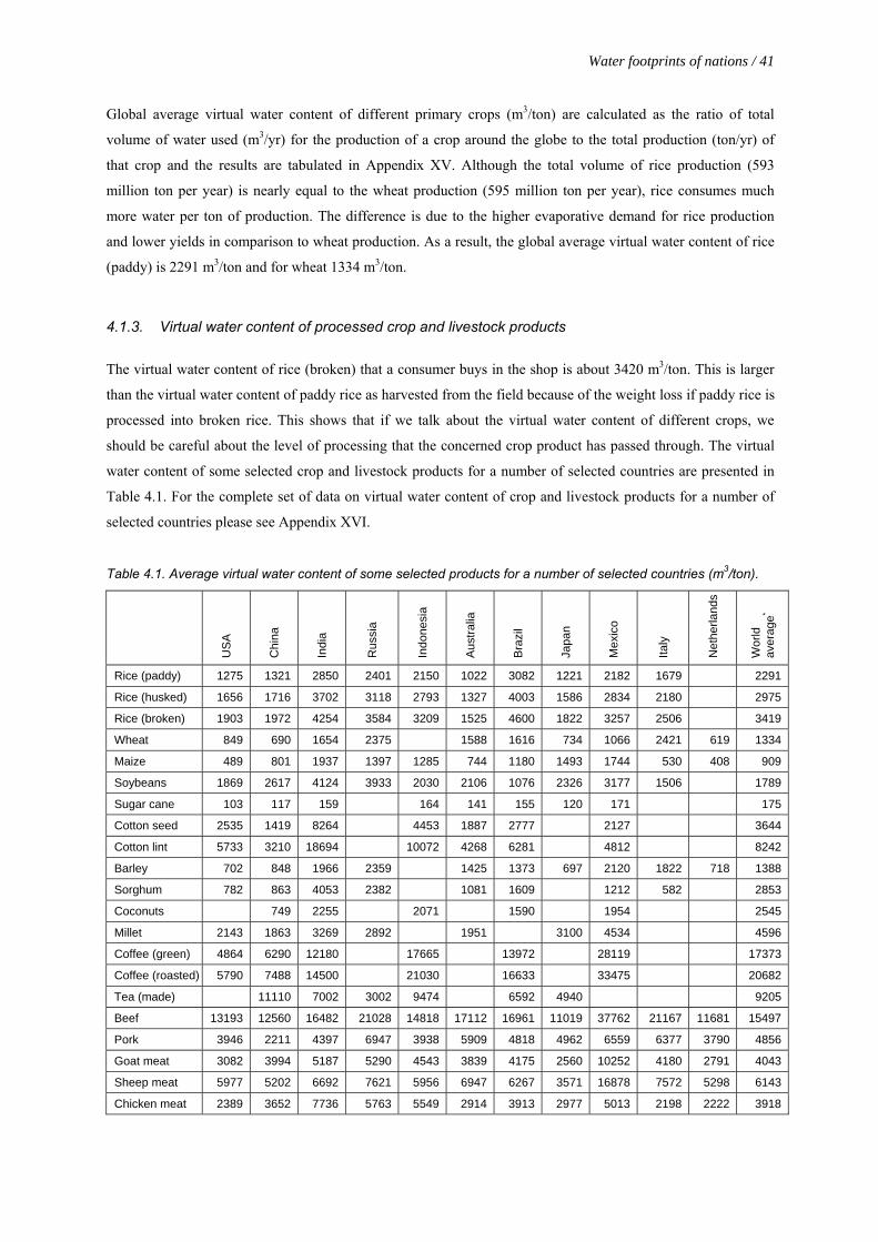
Water footprints of nations / 41
Global average virtual water content of different primary crops (m3/ton) are calculated as the ratio of total
volume of water used (m3/yr) for the production of a crop around the globe to the total production (ton/yr) of
that crop and the results are tabulated in Appendix XV. Although the total volume of rice production (593
million ton per year) is nearly equal to the wheat production (595 million ton per year), rice consumes much
more water per ton of production. The difference is due to the higher evaporative demand for rice production
and lower yields in comparison to wheat production. As a result, the global average virtual water content of rice
(paddy) is 2291 m3/ton and for wheat 1334 m3/ton.
4.1.3. Virtual water content of processed crop and livestock products
The virtual water content of rice (broken) that a consumer buys in the shop is about 3420 m3/ton. This is larger
than the virtual water content of paddy rice as harvested from the field because of the weight loss if paddy rice is
processed into broken rice. This shows that if we talk about the virtual water content of different crops, we
should be careful about the level of processing that the concerned crop product has passed through. The virtual
water content of some selected crop and livestock products for a number of selected countries are presented in
Table 4.1. For the complete set of data on virtual water content of crop and livestock products for a number of
selected countries please see Appendix XVI.
Table 4.1. Average virtual water content of some selected products for a number of selected countries (m3/ton).
US
A
Chi
na
Indi
a
Rus
sia
Indo
nesi
a
Aus
tralia
Bra
zil
Japa
n
Mex
ico
Italy
Net
herla
nds
Wor
ld
aver
age*
Rice (paddy) 1275 1321 2850 2401 2150 1022 3082 1221 2182 1679 2291
Rice (husked) 1656 1716 3702 3118 2793 1327 4003 1586 2834 2180 2975
Rice (broken) 1903 1972 4254 3584 3209 1525 4600 1822 3257 2506 3419
Wheat 849 690 1654 2375 1588 1616 734 1066 2421 619 1334
Maize 489 801 1937 1397 1285 744 1180 1493 1744 530 408 909
Soybeans 1869 2617 4124 3933 2030 2106 1076 2326 3177 1506 1789
Sugar cane 103 117 159 164 141 155 120 171 175
Cotton seed 2535 1419 8264 4453 1887 2777 2127 3644
Cotton lint 5733 3210 18694 10072 4268 6281 4812 8242
Barley 702 848 1966 2359 1425 1373 697 2120 1822 718 1388
Sorghum 782 863 4053 2382 1081 1609 1212 582 2853
Coconuts 749 2255 2071 1590 1954 2545
Millet 2143 1863 3269 2892 1951 3100 4534 4596
Coffee (green) 4864 6290 12180 17665 13972 28119 17373
Coffee (roasted) 5790 7488 14500 21030 16633 33475 20682
Tea (made) 11110 7002 3002 9474 6592 4940 9205
Beef 13193 12560 16482 21028 14818 17112 16961 11019 37762 21167 11681 15497
Pork 3946 2211 4397 6947 3938 5909 4818 4962 6559 6377 3790 4856
Goat meat 3082 3994 5187 5290 4543 3839 4175 2560 10252 4180 2791 4043
Sheep meat 5977 5202 6692 7621 5956 6947 6267 3571 16878 7572 5298 6143
Chicken meat 2389 3652 7736 5763 5549 2914 3913 2977 5013 2198 2222 3918

42 / Water footprints of nationso
US
A
Chi
na
Indi
a
Rus
sia
Indo
nesi
a
Aus
tralia
Bra
zil
Japa
n
Mex
ico
Italy
Net
herla
nds
Wor
ld
aver
age*
Eggs 1510 3550 7531 4919 5400 1844 3337 1884 4277 1389 1404 3340
Milk 695 1000 1369 1345 1143 915 1001 812 2382 861 641 990
Milk powder 3234 4648 6368 6253 5317 4255 4654 3774 11077 4005 2982 4602
Cheese 3457 4963 6793 6671 5675 4544 4969 4032 11805 4278 3190 4914
Leather (bovine) 14190 13513 17710 22575 15929 18384 18222 11864 40482 22724 12572 16656
* For the primary crops, world averages have been calculated as the ratio of the global water use for the production of a crop to the global production volume. For processed products, the global averages have been calculated as the ratio of the global virtual water trade volume to the global product trade volume.
In general livestock products have higher virtual water content than crop products. This is because a live animal
consumes a lot of feed crops, drinking water and service water in its lifetime before it produces some output. Let
us consider an example of beef produced in an industrial farming system. It takes in average 3 years before it is
slaughtered to produce about 200 kg of boneless beef. It consumes nearly 1300 kg of grains (wheat, oats, barley,
corn, dry peas, soybean meal and other small grains), 7200 kg of roughages (pasture, dry hay, silage and other
roughages), 24 cubic meter of water for drinking and 7 cubic meter of water for servicing. This means that to
produce one kilogram of boneless beef, we use about 6.5 kg of grain, 36 kg of roughages, and 155 litres of water
(only for drinking and servicing). Producing the volume of feed requires about 15340 litres of water in average.
With every step of food processing we loose part of the material as a result of selection and inefficiencies. The
higher we go up in the product chain, the higher will be the virtual water content of the product.
The units used so far to express the virtual water content of various products are in terms of cubic meters of
water per ton of the product (=litres/kg). A consumer might be more interested to know how much water it
consumes per unit of consumption. For example, what is the virtual water content of one cup of coffee, one glass
of wine, one A4 sheet of paper or a slice of bread? Table 4.2 gives the global average virtual water content of
some selected consumer goods expressed in water volumes per unit of product.
Table 4.2. Global average virtual water content of some selected products, per unit of product.
Product Virtual water
content (litres)
Product
Virtual water content (litres)
1 glass of beer (250 ml) 75 1 glass of wine (125 ml) 120
1 glass of milk (200 ml) 200 1 glass of apple juice (200 ml) 190
1 cup of coffee (125 ml) 140 1 glass of orange juice (200 ml) 170
1 cup of tea (250 ml) 35 1 bag of potato crisps (200 g) 185
1 slice of bread (30 g) 40 1 egg (40 g) 135
1 slice of bread (30 g) with cheese(10 g) 90 1 hamburger (150 g) 2400
1 potato (100 g) 25 1 tomato (70 g) 13
1 apple (100 g) 70 1 orange (100 g) 50
1 cotton T-shirt (medium sized, 500 g) 4100 1 pair of shoes (bovine leather) 8000
1 sheet of A4-paper (80 g/m2) 10 1 microchip (2 g) 32
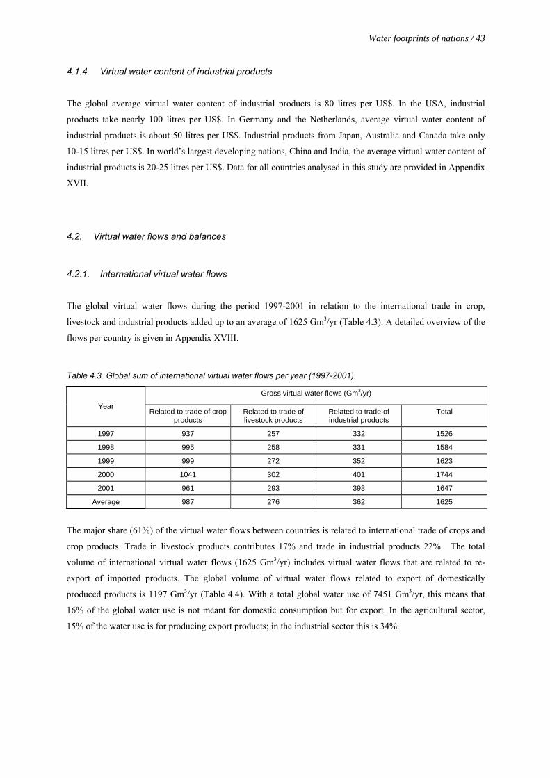
Water footprints of nations / 43
4.1.4. Virtual water content of industrial products
The global average virtual water content of industrial products is 80 litres per US$. In the USA, industrial
products take nearly 100 litres per US$. In Germany and the Netherlands, average virtual water content of
industrial products is about 50 litres per US$. Industrial products from Japan, Australia and Canada take only
10-15 litres per US$. In world’s largest developing nations, China and India, the average virtual water content of
industrial products is 20-25 litres per US$. Data for all countries analysed in this study are provided in Appendix
XVII.
4.2. Virtual water flows and balances
4.2.1. International virtual water flows
The global virtual water flows during the period 1997-2001 in relation to the international trade in crop,
livestock and industrial products added up to an average of 1625 Gm3/yr (Table 4.3). A detailed overview of the
flows per country is given in Appendix XVIII.
Table 4.3. Global sum of international virtual water flows per year (1997-2001).
Gross virtual water flows (Gm3/yr)
Year Related to trade of crop
products Related to trade of livestock products
Related to trade of industrial products
Total
1997 937 257 332 1526
1998 995 258 331 1584
1999 999 272 352 1623
2000 1041 302 401 1744
2001 961 293 393 1647
Average 987 276 362 1625
The major share (61%) of the virtual water flows between countries is related to international trade of crops and
crop products. Trade in livestock products contributes 17% and trade in industrial products 22%. The total
volume of international virtual water flows (1625 Gm3/yr) includes virtual water flows that are related to re-
export of imported products. The global volume of virtual water flows related to export of domestically
produced products is 1197 Gm3/yr (Table 4.4). With a total global water use of 7451 Gm3/yr, this means that
16% of the global water use is not meant for domestic consumption but for export. In the agricultural sector,
15% of the water use is for producing export products; in the industrial sector this is 34%.
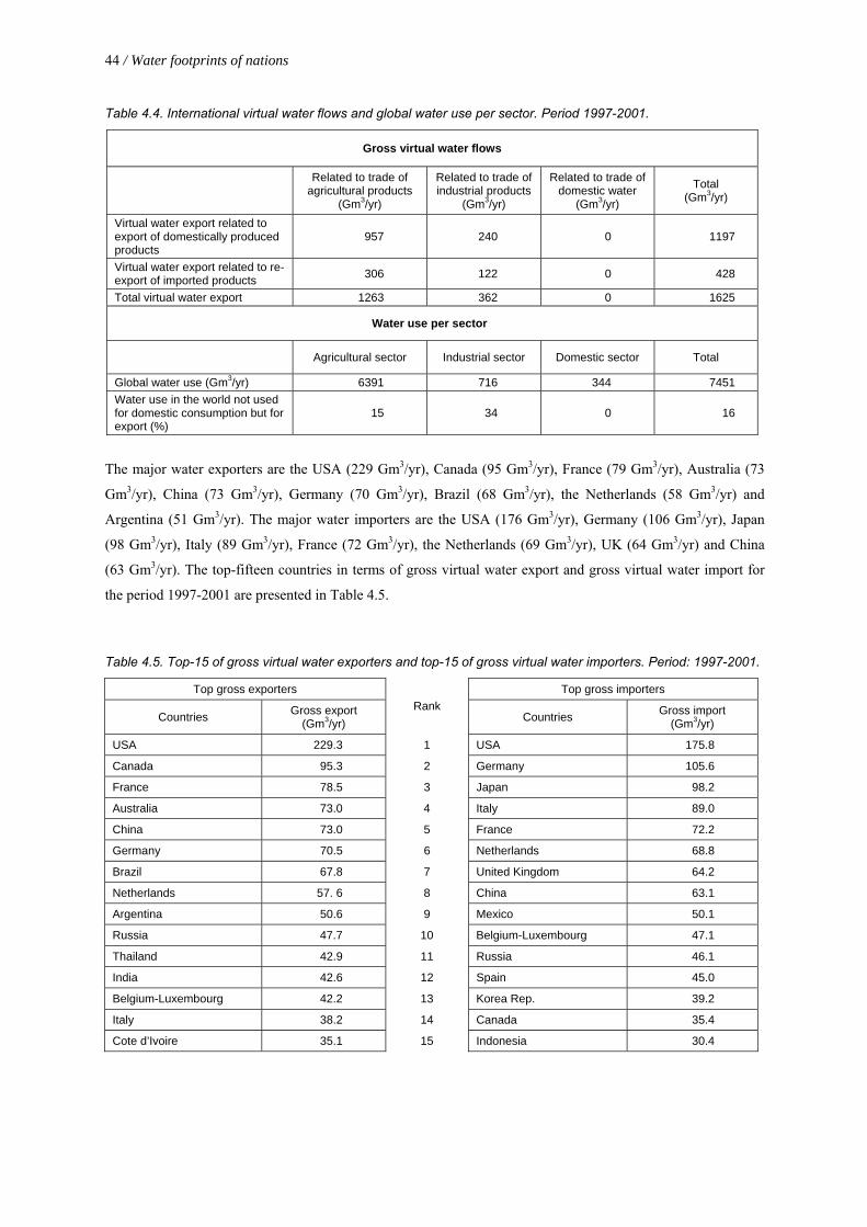
44 / Water footprints of nationso
Table 4.4. International virtual water flows and global water use per sector. Period 1997-2001.
Gross virtual water flows
Related to trade of agricultural products
(Gm3/yr)
Related to trade of industrial products
(Gm3/yr)
Related to trade of domestic water
(Gm3/yr)
Total (Gm3/yr)
Virtual water export related to export of domestically produced products
957 240 0 1197
Virtual water export related to re-export of imported products 306 122 0 428
Total virtual water export 1263 362 0 1625
Water use per sector
Agricultural sector Industrial sector Domestic sector Total
Global water use (Gm3/yr) 6391 716 344 7451 Water use in the world not used for domestic consumption but for export (%)
15 34 0 16
The major water exporters are the USA (229 Gm3/yr), Canada (95 Gm3/yr), France (79 Gm3/yr), Australia (73
Gm3/yr), China (73 Gm3/yr), Germany (70 Gm3/yr), Brazil (68 Gm3/yr), the Netherlands (58 Gm3/yr) and
Argentina (51 Gm3/yr). The major water importers are the USA (176 Gm3/yr), Germany (106 Gm3/yr), Japan
(98 Gm3/yr), Italy (89 Gm3/yr), France (72 Gm3/yr), the Netherlands (69 Gm3/yr), UK (64 Gm3/yr) and China
(63 Gm3/yr). The top-fifteen countries in terms of gross virtual water export and gross virtual water import for
the period 1997-2001 are presented in Table 4.5.
Table 4.5. Top-15 of gross virtual water exporters and top-15 of gross virtual water importers. Period: 1997-2001.
Top gross exporters Top gross importers
Countries Gross export (Gm3/yr)
Rank Countries Gross import
(Gm3/yr)
USA 229.3 1 USA 175.8
Canada 95.3 2 Germany 105.6
France 78.5 3 Japan 98.2
Australia 73.0 4 Italy 89.0
China 73.0 5 France 72.2
Germany 70.5 6 Netherlands 68.8
Brazil 67.8 7 United Kingdom 64.2
Netherlands 57. 6 8 China 63.1
Argentina 50.6 9 Mexico 50.1
Russia 47.7 10 Belgium-Luxembourg 47.1
Thailand 42.9 11 Russia 46.1
India 42.6 12 Spain 45.0
Belgium-Luxembourg 42.2 13 Korea Rep. 39.2
Italy 38.2 14 Canada 35.4
Cote d’Ivoire 35.1 15 Indonesia 30.4
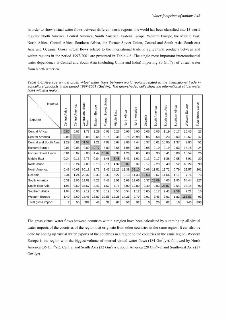
Water footprints of nations / 45
In order to show virtual water flows between different world regions, the world has been classified into 13 world
regions: North America, Central America, South America, Eastern Europe, Western Europe, the Middle East,
North Africa, Central Africa, Southern Africa, the Former Soviet Union, Central and South Asia, South-east
Asia and Oceania. Gross virtual flows related to the international trade in agricultural products between and
within regions in the period 1997-2001 are presented in Table 4.6. The single most important intercontinental
water dependency is Central and South Asia (including China and India) importing 80 Gm3/yr of virtual water
from North America.
Table 4.6. Average annual gross virtual water flows between world regions related to the international trade in agricultural products in the period 1997-2001 (Gm3/yr). The grey-shaded cells show the international virtual water flows within a region.
Importer
Exporter
Cen
tral A
frica
Cen
tral A
mer
ica
Cen
tral a
nd S
outh
A
sia
Eas
tern
Eur
ope
Form
er S
ovie
t Uni
on
Mid
dle
Eas
t
Nor
th A
frica
Nor
th A
mer
ica
Oce
ania
Sou
th A
mer
ica
Sou
th-e
ast A
sia
Sou
ther
n A
frica
Wes
tern
Eur
ope
Tota
l gro
ss e
xpor
t
Central Africa 0.80 0.07 1.73 1.29 0.03 0.26 0.96 0.90 0.06 0.05 1.19 0.17 16.45 23
Central America 0.08 3.13 3.88 0.65 6.14 0.38 0.75 23.98 0.06 0.58 0.23 0.03 10.67 47
Central and South Asia 1.29 0.81 31.53 1.21 4.08 6.67 3.86 4.44 0.37 0.61 16.90 1.37 9.80 51
Eastern Europe 0.01 0.08 0.69 10.77 4.80 2.65 1.08 0.55 0.08 0.10 0.19 0.03 14.15 24
Former Soviet Union 0.01 0.07 3.06 4.47 16.67 5.38 1.26 0.05 0.00 0.30 0.41 0.00 10.54 26
Middle East 0.24 0.11 2.73 0.84 1.46 8.45 3.43 1.01 0.13 0.17 1.86 0.05 6.91 20
North Africa 0.10 0.24 7.09 6.15 2.11 4.32 5.87 8.37 0.17 2.29 3.49 0.52 63.22 98
North America 0.46 40.65 80.18 1.71 2.43 11.22 11.38 35.10 0.96 11.51 13.72 0.79 25.57 201
Oceania 0.34 1.24 29.32 0.33 0.33 6.22 2.13 11.33 12.63 0.67 14.64 1.11 7.76 75
South America 0.39 3.06 19.82 4.23 4.46 8.92 5.08 19.65 0.37 28.09 4.63 1.93 54.44 127
South-east Asia 1.96 0.50 35.57 2.43 1.52 7.75 8.00 10.89 2.49 0.93 26.87 2.54 18.14 93
Southern Africa 1.04 0.06 2.12 0.38 0.19 0.53 0.54 1.12 0.05 0.17 2.41 2.59 7.21 16
Western Europe 1.40 2.60 15.45 18.87 10.56 12.28 14.26 9.79 0.91 2.45 2.61 1.82 183.51 93
Total gross import 7 50 202 43 38 67 53 92 6 20 62 10 245 895
The gross virtual water flows between countries within a region have been calculated by summing up all virtual
water imports of the countries of the region that originate from other countries in the same region. It can also be
done by adding up virtual water exports of the countries in a region to the countries in the same region. Western
Europe is the region with the biggest volume of internal virtual water flows (184 Gm3/yr), followed by North
America (35 Gm3/yr), Central and South Asia (32 Gm3/yr), South America (28 Gm3/yr) and South-east Asia (27
Gm3/yr).
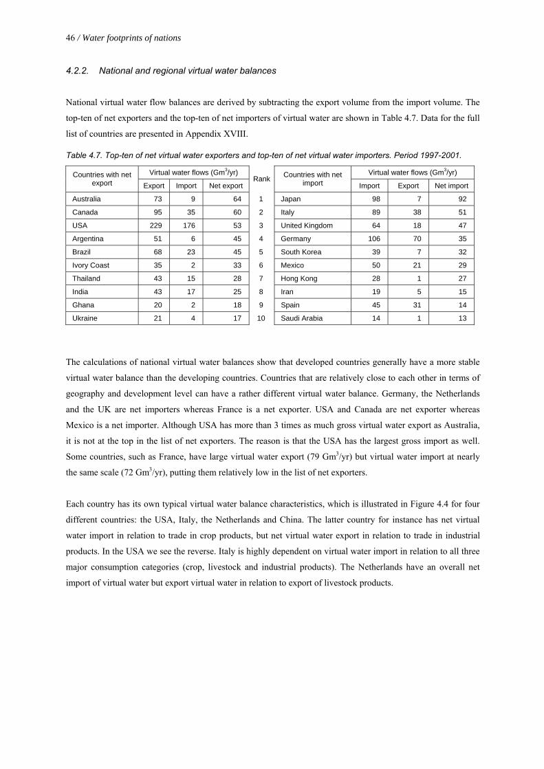
46 / Water footprints of nationso
4.2.2. National and regional virtual water balances
National virtual water flow balances are derived by subtracting the export volume from the import volume. The
top-ten of net exporters and the top-ten of net importers of virtual water are shown in Table 4.7. Data for the full
list of countries are presented in Appendix XVIII.
Table 4.7. Top-ten of net virtual water exporters and top-ten of net virtual water importers. Period 1997-2001.
Virtual water flows (Gm3/yr) Virtual water flows (Gm3/yr) Countries with net export Export Import Net export
Rank Countries with net import Import Export Net import
Australia 73 9 64 1 Japan 98 7 92
Canada 95 35 60 2 Italy 89 38 51
USA 229 176 53 3 United Kingdom 64 18 47
Argentina 51 6 45 4 Germany 106 70 35
Brazil 68 23 45 5 South Korea 39 7 32
Ivory Coast 35 2 33 6 Mexico 50 21 29
Thailand 43 15 28 7 Hong Kong 28 1 27
India 43 17 25 8 Iran 19 5 15
Ghana 20 2 18 9 Spain 45 31 14
Ukraine 21 4 17 10 Saudi Arabia 14 1 13
The calculations of national virtual water balances show that developed countries generally have a more stable
virtual water balance than the developing countries. Countries that are relatively close to each other in terms of
geography and development level can have a rather different virtual water balance. Germany, the Netherlands
and the UK are net importers whereas France is a net exporter. USA and Canada are net exporter whereas
Mexico is a net importer. Although USA has more than 3 times as much gross virtual water export as Australia,
it is not at the top in the list of net exporters. The reason is that the USA has the largest gross import as well.
Some countries, such as France, have large virtual water export (79 Gm3/yr) but virtual water import at nearly
the same scale (72 Gm3/yr), putting them relatively low in the list of net exporters.
Each country has its own typical virtual water balance characteristics, which is illustrated in Figure 4.4 for four
different countries: the USA, Italy, the Netherlands and China. The latter country for instance has net virtual
water import in relation to trade in crop products, but net virtual water export in relation to trade in industrial
products. In the USA we see the reverse. Italy is highly dependent on virtual water import in relation to all three
major consumption categories (crop, livestock and industrial products). The Netherlands have an overall net
import of virtual water but export virtual water in relation to export of livestock products.
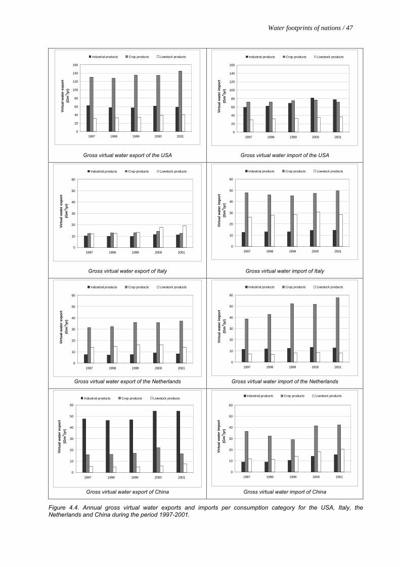
Water footprints of nations / 47
0
20
40
60
80
100
120
140
160
1997 1998 1999 2000 2001
Virt
ual w
ater
exp
ort
(Gm
3 /yr)
Industrial products Crop products Livestock products
0
20
40
60
80
100
120
140
160
1997 1998 1999 2000 2001
Virt
ual w
ater
impo
rt(G
m3 /y
r)
Industrial products Crop products Livestock products
Gross virtual water export of the USA Gross virtual water import of the USA
0
10
20
30
40
50
60
1997 1998 1999 2000 2001
Virt
ual w
ater
exp
ort
(Gm
3 /yr)
Industrial products Crop products Livestock products
0
10
20
30
40
50
60
1997 1998 1999 2000 2001
Virt
ual w
ater
impo
rt(G
m3 /y
r)
Industrial products Crop products Livestock products
Gross virtual water export of Italy Gross virtual water import of Italy
0
10
20
30
40
50
60
1997 1998 1999 2000 2001
Virt
ual w
ater
exp
ort
(Gm
3 /yr)
Industrial products Crop products Livestock products
0
10
20
30
40
50
60
1997 1998 1999 2000 2001
Virt
ual w
ater
impo
rt(G
m3 /y
r)
Industrial products Crop products Livestock products
Gross virtual water export of the Netherlands Gross virtual water import of the Netherlands
0
10
20
30
40
50
60
1997 1998 1999 2000 2001
Virt
ual w
ater
exp
ort
(Gm
3 /yr)
Industrial products Crop products Livestock products
0
10
20
30
40
50
60
1997 1998 1999 2000 2001
Virt
ual w
ater
impo
rt(G
m3 /y
r)
Industrial products Crop products Livestock products
Gross virtual water export of China Gross virtual water import of China
Figure 4.4. Annual gross virtual water exports and imports per consumption category for the USA, Italy, the Netherlands and China during the period 1997-2001.

48 / Water footprints of nationso
Average national virtual water balances over the period 1997-2001 are shown in Figure 4.5. The green coloured
countries in the map have net virtual water export, the red coloured ones net virtual water import. Figure 4.6
shows average virtual water balances over the period 1997-2001 at the level of 13 world regions. The figure also
shows the biggest virtual water flows between the different regions of the world insofar related to trade in
agricultural products. The regional analysis shows that the largest virtual water exporters are North America
(109 Gm3/yr) and South America (107 Gm3/yr) and the largest importers are Western Europe (152 Gm3/yr) and
Central and South Asia (151 Gm3/yr).
Net virtual water import (Gm3/yr)-100 - -50-50 - -25-25 - -10-10 - -5-5 - 00 - 55 - 2525 - 5050 - 100No Data
Figure 4.5. National virtual water balances related to the international trade of products. Period 1997-2001.
South America
Central America
North America
Southern Africa
North Africa
WesternEurope
Eastern EuropeFormer Soviet Union
Oceania
South-east Asia
Central and South Asia
MiddleEast
Central AfricaNet virtual water import (Gm3/yr)
-108-107-70-45-30-16-52131847150152No Data
Figure 4.6. Regional virtual water balances and net interregional virtual water flows related to the trade in agricultural products. Period: 1997-2001. Only the biggest net flows (>10 Gm3/yr) are shown.

Water footprints of nations / 49
4.2.3. Global virtual water flows by product
Bovine meat is the product with the single largest contribution to the global virtual water flows, followed by
soybean and wheat. The volumes of virtual water flows by product are presented in Appendix XIX. The major
products and their share to the total global virtual water flows are shown in the Figure 4.7.
Although the global volume of water consumption for producing rice is more than for wheat the global virtual
water flows related to the international trade of wheat are higher than for rice. However for some major rice
exporting countries the use of domestic water resources for producing rice for export can be significant. For
example, Thailand uses 28 Gm3/yr of water from its domestic resources to produce rice for export, which is
equal to 7% of the total renewable water resources.
Maize3%
Other41%
Raw sugar cane3%
Pork3%
Coffee7%
Rice6% Cotton
4%
Milk products2%
Barley2%
Cocoa9%
Wheat9%
Soyabean11%
Bovine meat13%
Other25%
Palm oil3%
Global volume of virtual water flow related to the trade of agricultural products = 1263 Gm3/yr
Figure 4.7. Contribution of various agricultural products to the global average virtual water flows related to the international trade of agricultural products over the period 1997-2001.
It varies very much from country to country which products and product groups contribute most to the ingoing
and outgoing virtual water flows (Table 4.8). The products behind the gross virtual water exports are generally
different from the products behind the virtual water imports, which means that ingoing and outgoing virtual
water flows can not simply be crossed out against each other. For example, in the USA 48% of the gross virtual
water export related to crop trade is from the export of oil crops and oils and 38% in the form of cereal products,
whereas 50% of its gross virtual water import related to crop trade is from the import of coffee, tea and cocoa
products. China is a net exporter of virtual water in terms of cereal products (8.5 Gm3/yr export and 5.8 Gm3/yr
import), but a net importer with respect to the oil crop, oil-cakes and oil products (3.1 Gm3/yr export and 24.4
Gm3/yr import). China is a net exporter of industrial products with 38.3 Gm3/yr which makes it a net exporter
country. France has nearly balanced virtual water flows with respect to the trade in crop products, but it mainly
exports cereals (24 Gm3/yr) and imports coffee, tea, cocoa, oil crops and oil-cakes (30.5 Gm3/yr).

50 / Water footprints of nationso
In the Netherlands the main products responsible for the import and export are from the same crop categories;
coffee, tea, cocoa, oil crops, oil-cakes and oil products. With the trade of products from these categories, it
imports 37 Gm3/yr and export 29 Gm3/yr. A large part of export is re-export of imported products (the
Netherlands even does not produce products like coffee, tea and cocoa). Australia mainly exports cereals (31
Gm3/yr) and imports coffee, tea, cocoa, oil crops, oil-cakes and oil products (3.0 Gm3/yr). Australia also has a
large net export of livestock products, which is 26 Gm3/yr. Thailand uses 28 Gm3/yr for producing rice for
export, which is quite significant if compared to the total agricultural water withdrawal in Thailand, which is 81
Gm3/yr.

Table 4.8. The contributions of individual products or product categories to the virtual water flows of a nation and their main trade partners for some selected nations. Period 1997-2001.
Gross export 134.6 43.4 46.1 17.4 48.3 34.5 38.4 32.4 12.9Oilcrops/oil-cakes/oil 65.9 Cereals 23.9 Cereals 31.1 Cereals 8.5 Cereals 31.1 Oilcrops/oil-cakes/oil 14.5 Cereals 29.2 Oilcrops/oil-cakes/oil 17.3 Cereals 4.2Cereals 50.8 Sugar/molasses 6.0 Oilcrops/oil-cakes/oil 6.1 Oilcrops/oil-cakes/oil 2.9 Oilcrops/oil-cakes/oil 13.4 Coffee/Tea/Cocoa 14.4 Sugar/molasses 5.1 Cereals 7.8 Oilcrops/oil-cakes/oil 3.6Textile fibres 9.1 Oilcrops/oil-cakes/oil 5.9 Sugar/molasses 4.3 Fruit/Veg/Juices 2.6 Fruit/Veg/Juices 2.4 Cereals 2.3 Fruit/Veg/Juices 2.5 Coffee/Tea 3.2 Fruit/Veg/Juices 2.0
Textile fibres 3.0 Coffee/Tea/Cocoa 1.8 Fruit/Veg/Juices 1.6 Textile fibres 1.5 Coffee/Tea/Cocoa 1.2Textile fibres 0.4 Spices etc 1.0
Soybean 56.9 Wheat 14.7 Sugar 16.4 Maize 4.1 Wheat 25.3 Cocoa 14.0 Rice 27.9 Soybean 8.8 Olive 2.8Maize 21.0 Sugar 4.6 Rice 8.5 Rice 3.6 Soybean 1.4 Soybean 6.9 Sugar 4.8 Rice 7.2 Rice 1.6Wheat 15.0 Maize 3.5 Wheat 4.3 Soybean 1.5 Barley 2.0 Tea 1.3 Coffee 0.9Cotton 9.1 Sugar 0.7 Coffee 1.9Rice 4.2 Wheat 0.4Mexico 21.2 Bel-lux 8.2 P.NewGunea 7.9 Korea Rep 3.4 USA 11.7 Germany 8.3 Indonesia 4.8 Indonesia 2.5 Germany 1.9Japan 21.0 Italy 4.6 Japan 7.1 Japan 2.0 Mexico 2.9 Bel-lux 5.6 Malaysia 2.7 China 2.1 France 1.7China 8.9 Germany 4.5 China 4.2 Indonesia 1.4 Japan 6.7 UK 4.7 Iran 2.6 USA 2.0 USA 1.6Canada 8.1 Netherlands 4.2 Indonesia 4.2 Malaysia 1.2 Iran 3.7 France 2.5 Japan 2.3 Saudi Arabia 2.0 Yemen 0.7Taiwan 7.3 Spain 3.4 Iran 3.3 China 3.4 China 2.2 Korea 1.8 UK 0.6
UK 2.9 Malaysia 2.2 Algeria 2.1 USA 1.9 Japan 1.6Gross export 35.5 13.2 26.4 5.6 17.4 15.1 2.9 3.4 14.9
Meat and ediable offals 17.0 Meat and ediable offals 4.8 Meat and ediable offals 17.2 Hides/skins/leather 2.7 Meat and ediable offals 8.3 Meat and ediable offals 7.5 Meat and ediable offals 2.4 Hides/skins/leather 10.3Hides/skins/leather 10.0 Dairy products 3.3 Hides/skins/leather 3.3 Meat and ediable offals 0.6 Live animals 5.8 Dairy products 1.5 Hides/skins/leather 0.7 Meat and ediable offals 2.0
Live animals 2.5 Dairy products 2.2 Live animals 0.6 Hides/skins/leather 2.0 Live animals 1.1 Dairy products 0.3 Dairy products 1.2Hides/skins/leather 1.3 Live animals 1.9 Hides/skins/leather 0.9 Live animals 0.2
Bovine 25.1 Bovine 6.3 Bovine 20.0 Bovine 2.6 Bovine 11.8 Bovine 4.4 Bovine 2.8 Bovine 11.0Swine 3.4 Dairy cow 3.2 Dairy cow 2.2 Swine 1.0 Swine 4.4 Swine 5.8 Laying hens 0.3 Swine 0.8Dairy cow 1.0 Swine 2.4 Sheep 2.1 Dairy cow 0.3 Dairy cow 2.9 Dairy cow 0.7
59.0 21.9 0.5 49.9 29.6 7.9 1.7 6.7 10.4Gross import 73.0 40.6 3.9 36.3 16.2 48.6 9.8 13.9 47.2
Coffee/Tea/Cocoa 36.8 Coffee/Tea/Cocoa 15.7 Coffee/Tea/Cocoa 1.8 Oilcrops/oil-cakes/oil 24.4 Coffee/Tea/Cocoa 5.4 Coffee/Tea/Cocoa 18.6 Oilcrops/oil-cakes/oil 4.4 Oilcrops/oil-cakes/oil 8.0 Oilcrops/oil-cakes/oil 21.4Oilcrops/oil-cakes/oil 11.2 Oilcrops/oil-cakes/oil 14.8 Oilcrops/oil-cakes/oil 1.4 Cereals 5.8 Oilcrops/oil-cakes/oil 3.4 Oilcrops/oil-cakes/oil 18.2 Textile fibres 3.7 Fruit/Veg/Juices 1.7 Coffee/Tea/Cocoa 10.2Cereals 9.3 Fruit/Veg/Juices 3.7 Cereals 0.3 Textile fibres 2.2 Sugar/Molasses 3.3 Cereals 6.5 Cereals 1.3 Cereals 1.4 Cereals 8.5Fruit/Veg/Juices 7.0 Cereals 2.6 Cereals 1.8 Spices etc 0.5 Textile fibres 3.3
Textile fibres 1.2 Fruit/Veg/Juices 1.4Textile fibres 0.6
Coffee 20.0 Cocoa 8.9 Soyabean 14.8 Sugar 3.2 Cocoa 15.9 Soyabean 3.6 Palm oil 5.0 Olive 13.3Cocoa 15.7 Coffee 6.7 Barley 2.5 Cocoa 2.9 Soyabean 8.3 Cotton 3.6 Wheat 1.3 Coffee 6.9Wheat 3.6 Soyabean 5.4 Sugar 1.6 Coffee 2.3 Wheat 3.2 Wheat 1.0 Soyabean 0.8 Wheat 6.7Oats 2.5 Rice 1.3 Wheat 1.5 Soyabean 2.2 Coffee 2.5 Sugar 0.9 Cotton 3.5Rice 1.7 Rice 1.5 Maize 0.9 Rice 0.7 Cocoa 3.3
Rice 0.8 Soyabean 3.3Canada 11.7 Cote d'ivore 5.1 USA 8.9 USA 8.1 Cote d'Ivore 5.7 USA 2.2 Malaysia 3.3 Tunisia 7.7Mexico 8.3 Brazil 4.2 Malaysia 2.6 Brazil 1.0 Germany 4.5 India 1.4 Indonesia 2.1 France 4.6Brazil 5.4 Spain 3.1 Brazil 2.6 USA 4.2 Australia 0.9 Argentina 1.3 Spain 4.2Cote d'ivore 4.7 India 1.5 India 2.1 France 4.2 Argentina 1.0 Pakistan 0.6 Brazil 2.1Colombia 3.5 USA 1.0 Thailand 2.2 Ghana 3.6 Greece 2.1India 2.0 Australia 4.3 Brazil 3.4 Argentina 1.9Thailand 1.9 Argentina 2.9 USA 1.7
Gross import 33.0 11.8 0.7 15.2 5.0 7.9 1.8 0.3 28.3Meat and ediable offals 14.6 Meat and ediable offals 6.4 Hides/skins/leather 13.1 Meat and ediable offals 2.9 Dairy cow 2.4 Hides/skins/leather 11.6Live animals 9.1 Dairy products 2.1 Meat and ediable offals 0.8 Hides/skins/leather 0.7 Meat and ediable offals 2.3 Meat and ediable offals 8.4Hides/skins/leather 6.0 Hides/skins/leather 0.9 Live animals 0.5 Live animals 0.8 Live animals 4.0Dairy products 0.9 Live animals 0.6 Hides/skins/leather 0.8 Dairy products 3.3Bovine 25.0 Bovine 4.7 Bovine 11.8 Bovine 3.9 Bovine 3.2 Bovine 17.4Swine 3.4 Swine 2.4 Swine 0.7 Swine 0.3 Dairy cow 2.4 Swine 4.8Dairy cow 0.9 Dairy cow 2.1 Sheep 0.6 Dairy cow 0.2 Swine 0.8 Dairy cow 3.3Horse 0.4 Sheep 0.7 Sheep 1.1
70.0 19.8 4.4 11.6 14.3 12.3 3.6 2.9 13.5Total gross export (Gm3/yr) 229.1 78.5 73.0 72.9 95.3 57.5 43.0 42.5 38.2Total gross import (Gm3/yr) 176.0 72.2 9.0 63.1 35.5 68.8 15.2 17.1 89.0
-53.1 -6.3 -64.0 -9.8 -59.8 11.3 -27.8 -25.4 50.8
Main livestock product groups
Main crop categories
Main livestock product groups
Main animal categories
Industrial products
Main crops
Main partners
Main animal categories
France China Canada
Main partners
Australia
Expo
rt (G
m3 /y
r)
Net import (Gm3/yr)
Livestock
Crop
Industrial products
Italy
Impo
rt (G
m3 /y
r)
Thailand India
Crop
livestock
Netherlands
Main crop categories
Main crops
USA

52 / Water footprints of nations o
4.3. Water footprints of nations
The global water footprint is 7450 Gm3/yr, which is 1240 m3/cap/yr in average. In absolute terms, India is the
country with the largest footprint in the world, with a total footprint of 987 Gm3/yr. However, while India
contributes 17% to the global population, the people in India contribute only 13% to the global water footprint.
On a relative basis, it is the people of the USA that have the largest water footprint, with 2480 m3/yr per capita,
followed by the people in south European countries such as Greece, Italy and Spain (2300-2400 m3/yr per
capita). High water footprints can also be found in Malaysia and Thailand. At the other side of the scale, the
Chinese people have a relatively low water footprint with an average of 700 m3/yr per capita.
The average per capita water footprints of nations are shown in Figure 4.8. The data are shown in Table 4.9 for
hundred selected countries and in Appendix XX for all countries considered in this study.
Figure 4.8. Average national water footprint per capita (m3/capita/yr). Green means that the nation’s water footprint is equal to or smaller than global average. Countries with red have a water footprint beyond the global average.
WFP(m3/cap/yr)600 - 800800 - 10001000 - 12001200 - 13001300 - 15001500 - 18001800 - 21002100 - 2500No Data
The size of the global water footprint is largely determined by the consumption of food and other agricultural
products (Figure 4.9). Our estimate of the contribution of agriculture to the total water use is even bigger than
most other statistics due to the inclusion of green water use (use of soil water).
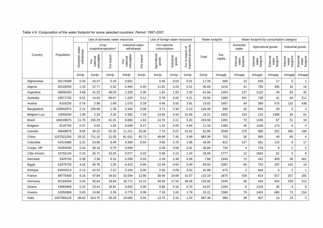
Table 4.9. Composition of the water footprint for some selected countries. Period: 1997-2001.
Use of domestic water resources Use of foreign water resources Water footprint Water footprint by consumption category
Crop evapotranspiration*
Industrial water withdrawal
For national consumption
Domestic water Agricultural goods Industrial goods
Dom
estic
wat
er
with
draw
al
For
natio
nal
cons
umpti
on
For e
xpor
t
For
natio
nal
cons
umpti
on
For e
xpor
t
Agr
icul
tura
l go
ods
Indu
stria
l go
ods
For r
e-ex
port
of
impo
rted
prod
ucts
Total Per capita
Inte
rnal
w
ater
fo
otpr
int
Inte
rnal
w
ater
fo
otpr
int
Ext
erna
l w
ater
fo
otpr
int
Inte
rnal
w
ater
fo
otpr
int
Ext
erna
l w
ater
fo
otpr
int Country
Population
Gm3/yr Gm3/yr Gm3/yr Gm3/yr Gm3/yr Gm3/yr Gm3/yr Gm3/yr Gm3/yr m3/cap/yr m3/cap/yr m3/cap/yr m3/cap/yr m3/cap/yr m3/cap/yr
Afghanistan 26179398 0.34 16.47 0.19 0.001 0.45 0.03 0.01 17.29 660 13 629 17 0 1
Algeria 30169250 1.23 22.77 0.32 0.494 0.25 11.91 0.29 0.31 36.69 1216 41 755 395 16 10
Argentina 36806250 4.68 41.31 48.03 2.328 0.30 1.81 1.53 2.30 51.66 1404 127 1122 49 63 42
Australia 19071705 6.51 14.03 68.67 1.229 0.12 0.78 4.02 4.21 26.56 1393 341 736 41 64 211
Austria 8103235 0.76 2.98 1.89 1.070 0.29 4.66 3.55 3.91 13.02 1607 94 368 575 132 438
Bangladesh 129942975 2.12 109.98 1.38 0.344 0.08 3.71 0.34 0.13 116.49 896 16 846 29 3 3
Belgium-Lux. 10659200 1.09 2.29 3.26 0.382 7.29 14.90 0.54 31.66 19.21 1802 103 215 1398 36 51
Brazil 169109675 11.76 195.29 61.01 8.666 1.63 14.76 3.11 5.20 233.59 1381 70 1155 87 51 18
Bulgaria 8125750 0.37 9.50 1.92 0.048 9.27 1.42 0.00 0.66 11.33 1395 45 1169 174 6 0
Canada 30649675 8.55 30.22 52.34 11.211 20.36 7.74 5.07 22.62 62.80 2049 279 986 252 366 166
China 1257521250 33.32 711.10 21.55 81.531 45.73 49.99 7.45 5.69 883.39 702 26 565 40 65 6
Colombia 41919368 5.31 23.08 9.40 0.358 0.04 4.60 0.70 1.96 34.05 812 127 551 110 9 17
Congo, DR 50264530 0.20 36.16 0.79 0.058 0.39 0.08 0.01 36.89 734 4 719 8 1 2
Côte d'Ivoire 15792145 0.19 26.71 33.83 0.077 0.02 0.96 0.13 1.24 28.06 1777 12 1692 61 5 8
Denmark 5329750 0.38 2.36 6.31 0.296 0.03 2.18 2.46 6.08 7.68 1440 72 442 409 56 461
Egypt 63375735 4.16 45.78 1.55 6.423 0.66 12.49 0.64 0.49 69.50 1097 66 722 197 101 10
Ethiopia 63540513 0.13 42.22 2.22 0.104 0.00 0.33 0.09 0.02 42.88 675 2 664 5 2 1
France 58775400 6.16 47.84 34.63 15.094 12.80 30.40 10.69 31.07 110.19 1875 105 814 517 257 182
Germany 82169250 5.45 35.64 18.84 18.771 13.15 49.59 17.50 38.48 126.95 1545 66 434 604 228 213
Ghana 19082858 0.15 23.44 18.81 0.054 0.00 0.86 0.16 0.70 24.67 1293 8 1229 45 3 8
Greece 10550968 0.83 14.80 3.35 0.775 0.08 7.18 1.62 1.79 25.21 2389 79 1403 680 73 154
India 1007369125 38.62 913.70 35.29 19.065 6.04 13.75 2.24 1.24 987.38 980 38 907 14 19 2
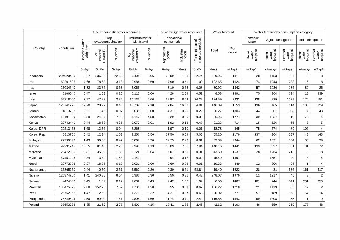
s
Use of domestic water resources Use of foreign water resources Water footprint Water footprint by consumption category
Crop evapotranspiration*
Industrial water withdrawal
For national consumption
Domestic water Agricultural goods Industrial goods
Dom
estic
wat
er
with
draw
al
For
natio
nal
cons
umpti
on
For e
xpor
t
For
natio
nal
cons
umpti
on
For e
xpor
t
Agr
icul
tura
l go
ods
Indu
stria
l go
ods
For r
e-ex
port
of
impo
rted
prod
ucts
Total Per capita
Inte
rnal
w
ater
fo
otpr
int
Inte
rnal
w
ater
fo
otpr
int
Ext
erna
l w
ater
fo
otpr
int
Inte
rnal
w
ater
fo
otpr
int
Ext
erna
l w
ater
fo
otpr
int Country
Population
Gm3/yr Gm3/yr Gm3/yr Gm3/yr Gm3/yr Gm3/yr Gm3/yr Gm3/yr Gm3/yr m3/cap/yr m3/cap/yr m3/cap/yr m3/cap/yr m3/cap/yr m3/cap/yr
Indonesia 204920450 5.67 236.22 22.62 0.404 0.06 26.09 1.58 2.74 269.96 1317 28 1153 127 2 8
Iran 63201525 4.68 78.58 3.18 0.984 0.60 17.90 0.51 1.03 102.65 1624 74 1243 283 16 8
Iraq 23034540 1.32 23.86 0.63 2.055 3.10 0.58 0.08 30.92 1342 57 1036 135 89 25
Israel 6166040 0.47 1.63 0.20 0.112 0.00 4.28 2.09 0.59 8.58 1391 75 264 694 18 339
Italy 57718000 7.97 47.82 12.35 10.133 5.60 59.97 8.69 20.29 134.59 2332 138 829 1039 176 151
Japan 126741225 17.20 20.97 0.40 13.702 2.10 77.84 16.38 4.01 146.09 1153 136 165 614 108 129
Jordan 4813708 0.21 1.45 0.07 0.035 0.00 4.37 0.21 0.22 6.27 1303 44 301 908 7 43
Kazakhstan 15191620 0.59 24.87 7.92 1.147 4.58 0.29 0.06 0.33 26.96 1774 39 1637 19 76 4
Kenya 29742440 0.44 18.63 4.35 0.079 0.01 1.92 0.16 0.47 21.23 714 15 626 65 3 5
Korea, DPR 22213458 1.68 12.76 0.04 2.268 1.97 0.10 0.01 18.78 845 75 574 89 102 4
Korea, Rep 46813750 6.42 12.34 1.53 2.256 0.56 27.50 6.69 5.06 55.20 1179 137 264 587 48 143
Malaysia 22990590 1.43 36.58 18.47 0.867 0.90 12.73 2.28 8.81 53.89 2344 62 1591 554 38 99
Mexico 97291745 13.55 81.48 12.26 2.998 1.13 35.09 7.05 7.94 140.16 1441 139 837 361 31 72
Morocco 28472000 0.81 35.99 1.33 0.224 0.04 6.07 0.51 0.31 43.60 1531 28 1264 213 8 18
Myanmar 47451298 0.34 73.89 1.53 0.149 0.94 0.17 0.02 75.49 1591 7 1557 20 3 4
Nepal 22772793 0.27 18.35 0.19 0.031 0.00 0.60 0.08 0.01 19.33 849 12 806 26 1 4
Netherlands 15865250 0.44 0.50 2.51 2.562 2.20 9.30 6.61 52.84 19.40 1223 28 31 586 161 417
Nigeria 125374700 1.41 240.38 8.54 0.383 0.30 5.59 0.31 0.43 248.07 1979 11 1917 45 3 2
Norway 4474000 0.45 1.09 0.17 1.032 0.43 2.42 1.57 1.02 6.56 1467 101 244 541 231 350
Pakistan 136475525 2.88 152.75 7.57 1.706 1.28 8.55 0.33 0.67 166.22 1218 21 1119 63 12 2
Peru 25752968 1.47 12.59 1.82 1.379 0.32 4.21 0.37 0.69 20.02 777 57 489 163 54 14
Philippines 75749645 4.50 99.09 7.61 0.805 1.69 11.74 0.71 2.40 116.85 1543 59 1308 155 11 9
Poland 38653288 1.85 21.62 2.78 6.890 4.15 10.41 1.85 2.45 42.62 1103 48 559 269 178 48

Use of domestic water resources Use of foreign water resources Water footprint Water footprint by consumption category
Crop evapotranspiration*
Industrial water withdrawal
For national consumption
Domestic water Agricultural goods Industrial goods
Dom
estic
wat
er
with
draw
al
For
natio
nal
cons
umpti
on
For e
xpor
t
For
natio
nal
cons
umpti
on
For e
xpor
t
Agr
icul
tura
l go
ods
Indu
stria
l go
ods
For r
e-ex
port
of
impo
rted
prod
ucts
Total Per capita
Inte
rnal
w
ater
fo
otpr
int
Inte
rnal
w
ater
fo
otpr
int
Ext
erna
l w
ater
fo
otpr
int
Inte
rnal
w
ater
fo
otpr
int
Ext
erna
l w
ater
fo
otpr
int Country
Population
Gm3/yr Gm3/yr Gm3/yr Gm3/yr Gm3/yr Gm3/yr Gm3/yr Gm3/yr Gm3/yr m3/cap/yr m3/cap/yr m3/cap/yr m3/cap/yr m3/cap/yr m3/cap/yr
Portugal 9997250 1.09 8.00 1.47 1.411 0.62 10.55 1.59 2.64 22.63 2264 109 800 1055 141 159
Romania 22450998 2.04 29.03 2.51 3.527 4.75 3.99 0.34 0.80 38.92 1734 91 1293 178 157 15
Russia 145878750 14.34 201.26 8.96 13.251 34.83 41.33 0.80 3.94 270.98 1858 98 1380 283 91 5
Saudi Arabia 20503670 1.61 10.42 0.42 0.181 0.01 12.11 1.58 0.62 25.90 1263 78 508 591 9 77
South Africa 42387403 2.43 27.32 6.05 1.123 0.40 7.18 1.42 2.10 39.47 931 57 644 169 26 33
Spain 40417948 4.24 50.57 17.44 5.567 1.73 27.11 6.50 11.37 93.98 2325 105 1251 671 138 161
Sri Lanka 18335500 0.25 21.72 2.29 0.165 0.09 1.32 0.24 0.26 23.69 1292 14 1185 72 9 13
Sudan 30832808 0.89 66.62 7.47 0.189 0.04 0.48 0.07 0.07 68.25 2214 29 2161 15 6 2
Sweden 8868050 1.07 4.49 1.42 1.166 0.45 4.52 3.12 2.62 14.37 1621 121 507 509 132 352
Switzerland 7165250 0.45 0.97 0.23 1.057 0.33 5.59 3.98 2.56 12.05 1682 63 136 780 148 555
Tanzania 33299168 0.11 36.39 3.15 0.024 0.00 0.90 0.08 0.08 37.51 1127 3 1093 27 1 3
Thailand 60487800 1.83 120.17 38.49 1.239 0.55 8.73 2.49 3.90 134.46 2223 30 1987 144 20 41
Turkey 66849750 5.38 84.05 9.81 2.731 1.07 13.68 2.11 2.43 107.95 1615 80 1257 205 41 32
Turkmenistan 5184250 0.38 8.39 1.07 0.118 0.05 0.18 0.07 0.05 9.14 1764 74 1619 36 23 13
Ukraine 49700750 4.60 54.14 10.09 3.673 9.71 2.72 0.26 1.21 65.40 1316 93 1089 55 74 5
United Kingdom 58669403 2.21 12.79 3.38 6.673 1.46 34.73 16.67 12.83 73.07 1245 38 218 592 114 284
USA 280343325 60.80 334.24 138.96 170.777 44.72 74.91 55.29 45.62 696.01 2483 217 1192 267 609 197
Uzbekistan 24567500 2.68 18.93 6.24 1.151 1.06 0.23 0.35 24.04 979 109 771 43 47 9
Venezuela 23937750 2.80 12.42 1.28 0.360 0.13 4.86 0.70 0.76 21.14 883 117 519 203 15 29
Viet Nam 78020938 3.77 85.16 11.00 11.280 2.27 0.85 0.29 103.33 1324 48 1091 29 145 11
Global total/average 5994251631 344 5434 957 476 240 957 240 427 7452 1243 57 907 160 79 40* Includes both blue and green water use in agriculture.

56 / Water footprints of nations a
85.8%
4.6%
9.6%
Water footprint related to consumption of industrial goods
Water footprint related to domestic water consumption
Water footprint related to consumption of agricultural goods
Figure 4.9. Global water footprint per consumption category.
The major factors determining the per capita water footprint of a country are:
− the average consumption volume per capita, generally related to gross national income per country,
− the consumption habits of the inhabitants of the country,
− climate, in particular evaporative demand, and
− agricultural practice.
In rich countries, people generally consume more goods and services, which immediately translate into
increased water footprints. But it is not consumption volume alone that determines the water demand of people.
The composition of the consumption package is relevant too, because some goods in particular require a lot of
water (bovine meat, rice). In many poor countries it is a combination of unfavourable climatic conditions (high
evaporative demand) and bad agricultural practice (resulting in low water productivity) that contributes to a high
water footprint.
The influence of the various determinants varies from country to country. The water footprint of USA is high
(2480 m3/cap/yr) partly because of large meat consumption per capita and high consumption of industrial
products. The water footprint of Iran is relatively high (1624 m3/cap/yr) partly because of low yields in crop
production and partly because of high evapotranspiration. In the USA the industrial component of the water
footprint is 806 m3/cap/yr whereas in Iran it is only 24 m3/cap/yr.
The aggregated external water footprints of nations in the world constitute 16% of the total global water
footprint (Figure 4.10). However, the share of the external water footprint strongly varies from country to
country. Some African countries, such as Sudan, Mali, Nigeria, Ethiopia, Malawi and Chad have hardly any
external water footprint, simply because they have little import. Some European countries on the other hand, e.g.
Italy, Germany, the UK and the Netherlands have external water footprints contributing 50-80% to the total
water footprint. The agricultural products that contribute most to the external water footprints of nations are:
bovine meat, soybean, wheat, cocoa, rice, cotton and maize.
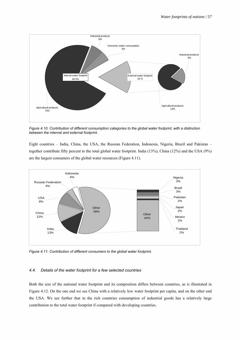
Water footprints of nations / 57
Domestic water consumption5%
Industrial products6%
Agricultural products73%
External water footprint16 %
Industrial products3%
Agricultural products13%
Internal water footprint84.0%
Figure 4.10. Contribution of different consumption categories to the global water footprint, with a distinction between the internal and external footprint.
Eight countries – India, China, the USA, the Russian Federation, Indonesia, Nigeria, Brazil and Pakistan –
together contribute fifty percent to the total global water footprint. India (13%), China (12%) and the USA (9%)
are the largest consumers of the global water resources (Figure 4.11).
Mexico2%
Thailand2%
Other44%
Other58%
Japan2%
Pakistan2%
Brazil3%
Nigeria3%
Indonesia4%
Russian Federation4%
USA9%
China12%
India13%
Figure 4.11. Contribution of different consumers to the global water footprint.
4.4. Details of the water footprint for a few selected countries
Both the size of the national water footprint and its composition differs between countries, as is illustrated in
Figure 4.12. On the one end we see China with a relatively low water footprint per capita, and on the other end
the USA. We see further that in the rich countries consumption of industrial goods has a relatively large
contribution to the total water footprint if compared with developing countries.
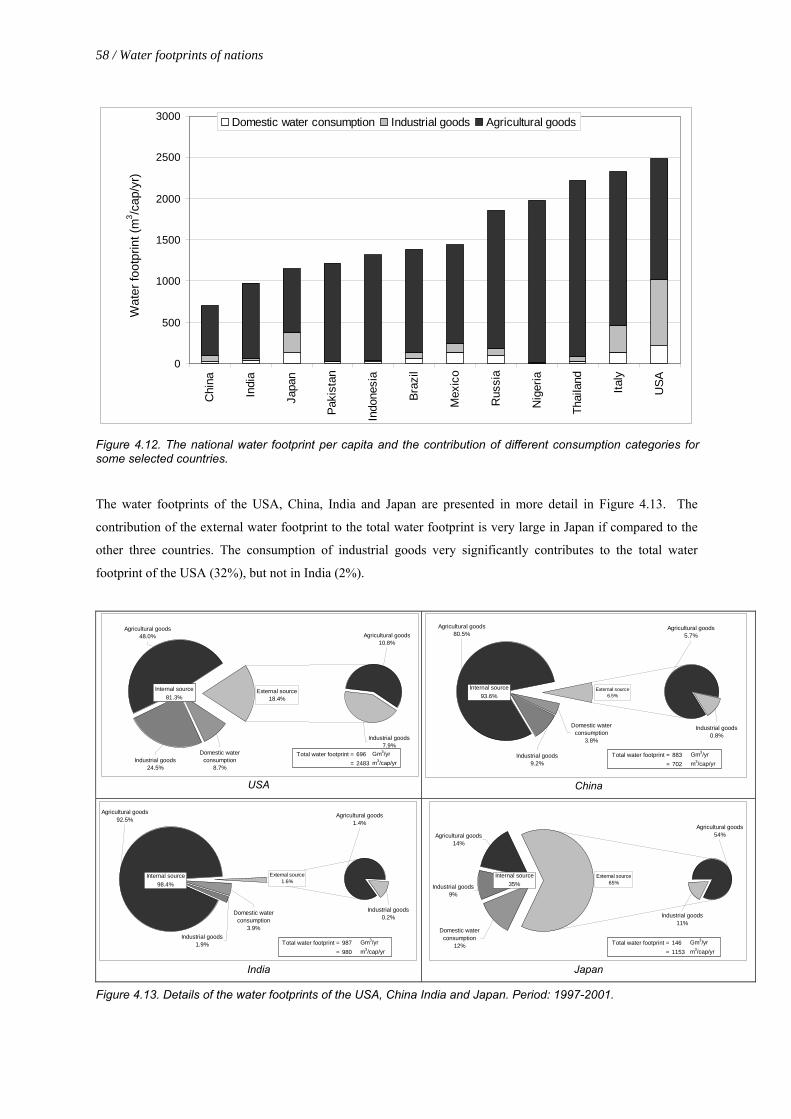
58 / Water footprints of nations a
0
500
1000
1500
2000
2500
3000
Chi
na
Indi
a
Japa
n
Paki
stan
Indo
nesi
a
Braz
il
Mex
ico
Rus
sia
Nig
eria
Thai
land
Italy
USA
Wat
er fo
otpr
int (
m3 /c
ap/y
r)Domestic water consumption Industrial goods Agricultural goods
Figure 4.12. The national water footprint per capita and the contribution of different consumption categories for some selected countries.
The water footprints of the USA, China, India and Japan are presented in more detail in Figure 4.13. The
contribution of the external water footprint to the total water footprint is very large in Japan if compared to the
other three countries. The consumption of industrial goods very significantly contributes to the total water
footprint of the USA (32%), but not in India (2%).
Industrial goods7.9%
External source18.4%
Agricultural goods48.0%
Domestic water consumption
8.7%Industrial goods
24.5%
Agricultural goods10.8%
Internal source81.3%
Total water footprint = 696 Gm3/yr= 2483 m3/cap/yr
USA China
India Japan
Industrial goods0.8%
External source6.5%
Agricultural goods80.5%
Domestic water consumption
3.8%
Industrial goods9.2%
Agricultural goods5.7%
Internal source93.6%
Total water footprint = 883 Gm3/yr= 702 m3/cap/yr
Industrial goods0.2%
External source1.6%
Agricultural goods92.5%
Domestic water consumption
3.9%Industrial goods
1.9%
Agricultural goods1.4%
Internal source98.4%
Total water footprint = 987 Gm3/yr= 980 m3/cap/yr
Industrial goods11%
External source65%
Agricultural goods14%
Domestic water consumption
12%
Industrial goods9%
Agricultural goods54%
Internal source35%
Total water footprint = 146 Gm3/yr= 1153 m3/cap/yr
Figure 4.13. Details of the water footprints of the USA, China India and Japan. Period: 1997-2001.

Water footprints of nations / 59
4.5. Correlation between water footprints of nations and a few selected determinants
4.5.1. Water footprints in relation to gross national income
The national water footprints related to domestic water consumption have been plotted against gross national
income (GNI) per capita in Figure 4.14. The same has been done for national water footprints due to the
consumption of industrial products in Figure 4.15. In both cases we see a positive relation between water
footprint per capita and GNI per capita. Note that we have used logarithmic scales in the plots. The effect of
GNI on water footprint diminishes at larger GNI per capita. National water footprints related to the consumption
of agricultural products have been plotted against GNI per capita in Figure 4.16. We do not see a positive
relation as in the previous two figures. The reason is that other factors – climate, agricultural practice and
consumption pattern – interfere to such extent that these factors should be filtered out first before we can see the
individual effect of GNI per capita. We have not done that in this phase of the study yet.

60 / Water footprints of nations a
Switzerland
Norway
Japan
USA
Denmark
Iceland
SwedenAustria
Germany
Netherlands
France
Finland
UK
CanadaAustralia
Italy
Kuwait
Israel
Spain
CyprusGreece
Portugal
BahrainKorea, Rep
Saudi Arabia
Argentina
Oman
Czech Republic
EcuadorMexico
ChileHungary
Poland
VenezuelaLebanon
Brazil
Panama
Mauritius
Costa Rica
Malaysia
Gabon
Botswana
South Africa
TurkeyLatviaBelizeJamaica
Fiji
Colombia
Peru
TunisiaThailand
Suriname
El Salvador
Russia
Guatemala
Jordan
IranRomania
Paraguay
Algeria
Belarus
Swaziland
Cape Verde
Morocco
Albania
Philippines
Bolivia
Syria
Sri Lanka
Guyana
Honduras
China
UkraineTurkmenistan
Papua New Guinea
Côte d'Ivoire
Georgia
Indonesia
Armenia
UzbekistanAzerbaijan
Zimbabwe
Senegal
AngolaHaiti
Pakistan
India
Yemen
Mauritania
Benin
Viet Nam
Bangladesh
Nicaragua
Moldova
Ghana
Gambia
Sudan
Kyrgyzstan
Laos
Central African Republic
Nigeria
Cambodia
Rwanda
Tanzania
Nepal
Burkina Faso
Chad
Malawi
Tajikistan
Sierra Leone
Liberia
Burundi
Ethiopia
Congo, DRy = 0.74x0.53
R2 = 0.51
1
10
100
1000
10 100 1000 10000 100000
GNI per capita (US$/cap/yr)
Wat
er fo
otpr
int r
elat
ed to
dom
estic
wat
erco
nsum
ptio
n (m
3 /cap
/yr)
Figure 4.14. Relation between water footprint due to domestic water consumption and gross national income.
Figure 4.15. Relation between water footprint due to consumption of industrial goods and gross national income.
Figure 4.16.Relation between water footprint due to consumption of agricultural products and gross national income.
Congo DR
Ethiopia
Burundi
Liberia
Sierra Leone
Tajikistan
Malawi
Chad
Mozambique
Burkina Faso
Nepal
TanzaniaMadagascar
Rwanda
Cambodia
Nigeria
Central African Republic
Laos
Kyrgyzstan
SudanZambia
GambiaGhana
Kenya
Nicaragua
Bangladesh
Viet Nam
Benin
Mauritania
YemenIndia
Pakistan
HaitiAngola
SenegalBhutan
Zimbabwe
Azerbaijan
Cameroon
Uzbekistan
Armenia
IndonesiaGeorgiaCôte d'Ivoire
Ukraine
China
Honduras
Guyana
Sri Lanka
Syria
BoliviaPhilippines
Albania
Morocco
Kazakhstan
Swaziland
Belarus
Bulgaria
AlgeriaParaguay
Romania
Iran
Jordan
Guatemala
Russia
El SalvadorSuriname
ThailandTunisiaNamibiaPeru
Colombia
Jamaica
BelizeLatvia
Turkey
Lithuania
South AfricaBotswana
Gabon
MalaysiaMauritius
PanamaBrazil
Lebanon
Venezuela
Poland
Hungary
Chile
Mexico
Ecuador
Trinidad and TobagoCzech Republic
Oman
ArgentinaSaudi Arabia
Korea, Rep.
Barbados
MaltaBahrain
Portugal
Greece
SpainIsrael
Kuwait
Italy
Australia
Canada
UKFinlandFrance
Netherlands
Germany
AustriaSwedenIceland
Denmark
USA
Japan
NorwaySwitzerland
y = 0.21x0.73
R2 = 0.62
1
10
100
1000
10 100 1000 10000 100000
GNI per capita (US$/cap/yr)
Wat
er fo
otpr
int r
elat
ed to
con
sum
ptio
n of
in
dust
rial g
oods
(m3 /c
ap/y
r)
Ethiopia
Burundi
Liberia
Sierra LeoneTajikistan
Malawi
Chad
Burkina Faso
Nepal
Mali
Tanzania
Madagascar
Rwanda
Cambodia
Nigeria
Laos
Togo
Sudan
Zambia
GambiaGhanaMoldova
KenyaNicaragua
Bangladesh
Viet Nam
Benin
Mauritania
Yemen
India
Pakistan
Haiti
Angola
Senegal
BhutanZimbabwe
Azerbaijan
Cameroon
Uzbekistan
Armenia
Indonesia
Georgia
Côte d'Ivoire
Papua New Guinea
Turkmenistan
Ukraine
China
Honduras
Guyana
Sri Lanka
Syria
BoliviaAlbania
Morocco
Kazakhstan
Cape Verde
SwazilandBelarus
Bulgaria
Paraguay
RomaniaIran
Jordan
Guatemala
Russia
El Salvador
Suriname
Thailand
Tunisia
NamibiaColombia
Jamaica
Belize
Latvia
Turkey
Lithuania
South Africa
Botswana
Gabon
Malaysia
Mauritius
Panama
BrazilLebanon
Venezuela
PolandHungary
Chile
Mexico
Ecuador
Czech Republic
Oman
ArgentinaSaudi Arabia
Korea RepBarbados
Malta
Bahrain
Portugal
Greece
CyprusSpain
Israel
Kuwait
Italy
Australia
Canada
UK
FinlandFrance
Netherlands
GermanyAustria
Sweden
Iceland
Denmark
USA
JapanNorway
Switzerland
0
500
1000
1500
2000
2500
100 1000 10000 100000GNI per capita (US$/cap/yr)
Wat
er fo
otpr
int r
elat
ed to
con
sum
ptio
n of
ag
ricul
tura
l goo
ds (m
3 /cap
/yr)
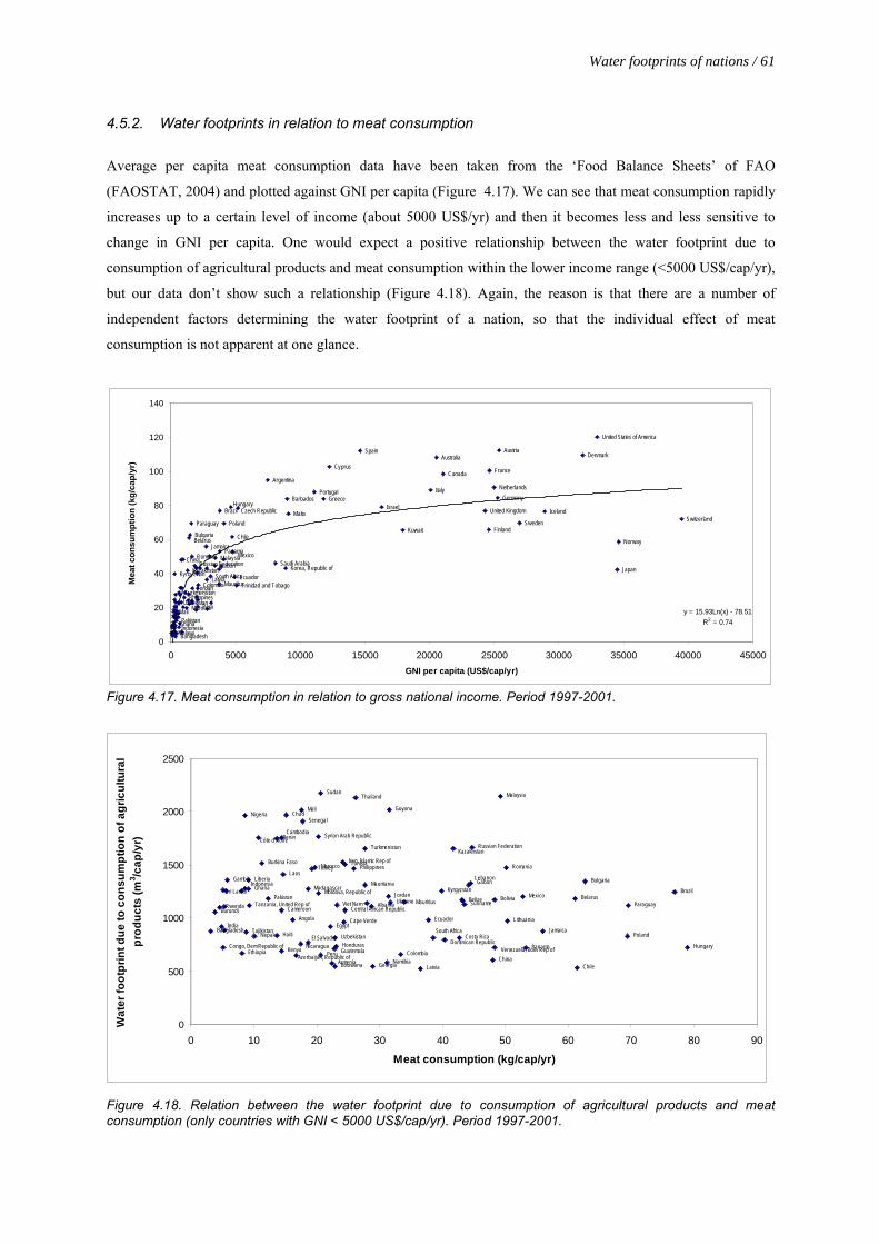
Water footprints of nations / 61
4.5.2. Water footprints in relation to meat consumption
Average per capita meat consumption data have been taken from the ‘Food Balance Sheets’ of FAO
(FAOSTAT, 2004) and plotted against GNI per capita (Figure 4.17). We can see that meat consumption rapidly
increases up to a certain level of income (about 5000 US$/yr) and then it becomes less and less sensitive to
change in GNI per capita. One would expect a positive relationship between the water footprint due to
consumption of agricultural products and meat consumption within the lower income range (<5000 US$/cap/yr),
but our data don’t show such a relationship (Figure 4.18). Again, the reason is that there are a number of
independent factors determining the water footprint of a nation, so that the individual effect of meat
consumption is not apparent at one glance.
Switzerland
Norway
Japan
United States of America
Denmark
Iceland
Sweden
Austria
GermanyNetherlands
France
Finland
United Kingdom
Canada
Australia
Italy
Kuwait
Israel
Spain
Cyprus
GreecePortugal
Malta
Barbados
Korea, Republic ofSaudi Arabia
Argentina
Czech Republic
Trinidad and TobagoEcuador
Mexico
Chile
Hungary
Poland
Brazil
Panama
Mauritius
MalaysiaGabon
South AfricaLatvia
Jamaica
Colombia
Peru
Russian Federation
Jordan
Romania
Paraguay
BulgariaBelarus
Kazakhstan
MoroccoPhilippines
China
Turkmenistan
Indonesia
Uzbekistan
Pakistan
Bangladesh
Ghana
Kyrgyzstan
Mali
Malawi
y = 15.93Ln(x) - 78.51R2 = 0.74
0
20
40
60
80
100
120
140
0 5000 10000 15000 20000 25000 30000 35000 40000 45000GNI per capita (US$/cap/yr)
Mea
t con
sum
ptio
n (k
g/ca
p/yr
)
Figure 4.17. Meat consumption in relation to gross national income. Period 1997-2001.
Hungary
Brazil
Paraguay
Poland
Bulgaria
Chile
Belarus
Jamaica
Panama
Mexico
Lithuania
Romania
Malaysia
Venezuela, Boliv Rep of
Bolivia
China
Russian Federation
GabonLebanon
SurinameBelize
Costa Rica
Kazakhstan
Dominican Republic
Kyrgyzstan
South Africa
Ecuador
Latvia
Mauritius
Colombia
Ukraine
Guyana
Jordan
NamibiaGeorgia
Albania
Turkmenistan
Mauritania
Thailand
PhilippinesTunisia
Central African Republic
Cape Verde
Iran, Islamic Rep of
Viet Nam
Honduras
Botswana
Uzbekistan
Guatemala
Armenia
Egypt
Peru
Sudan
Syrian Arab Republic
Moldova, Republic of
MoroccoTurkey
El Salvador
Madagascar
Senegal
Mali
Nicaragua
Azerbaijan, Republic of
Angola
Chad
Laos
Cameroon
Kenya
Cambodia
Haiti
Benin
Pakistan
Burkina Faso
Côte d'Ivoire
Nepal
Tanzania, United Rep of
GhanaLiberia
Tajikistan
Indonesia
Nigeria
Ethiopia
Gambia
Sri Lanka
Congo, Dem Republic of
India
RwandaBurundi
Bangladesh
0
500
1000
1500
2000
2500
0 10 20 30 40 50 60 70 80 9
Meat consumption (kg/cap/yr)
Wat
er fo
otpr
int d
ue to
con
sum
ptio
n of
agr
icul
tura
l pr
oduc
ts (m
3 /cap
/yr)
0
Figure 4.18. Relation between the water footprint due to consumption of agricultural products and meat consumption (only countries with GNI < 5000 US$/cap/yr). Period 1997-2001.

62 / Water footprints of nations a
4.5.3. Water footprints in relation to climate
The evaporative demand in a country determines the natural volume of water needed to grow crops. One would
expect that warmer countries have a relatively high water footprint related to the consumption of foods produced
within the country. Figure 4.19 shows that this is indeed true for nations such as Senegal, Mali, Sudan and Chad.
The overall picture however is diffuse, which is caused by the fact that climate is not the sole determinant of the
internal water footprint. Countries such as Bahrain, Kuwait and Qatar for instance have a high evaporative
demand but a low internal water footprint, because the major share of their agricultural demands are met by
import from outside.
Senegal
Mauritania
Saudi Arabia
KuwaitBahrain
Qatar
Mali
Sudan
Somalia
Burkina Faso
Iraq
Libya
Gambia
Chad
Algeria
Oman
Syria
JordanYemen
Nigeria
Egypt
Cape Verde
Benin
Zambia
Zimbabwe
Pakistan
South AfricaKenya
Ghana
Israel
Barbados
Namibia
Iran
Australia
Sri Lanka
Guyana
Dominican Republic
Paraguay
Angola
Venezuela
Mozambique
Botswana
Morocco
Mexico
Turkmenistan
Malawi
Thailand
Cuba
Jamaica
Bolivia
Lebanon
Haiti
Swaziland
CyprusUzbekistan
CambodiaCôte d'Ivoire
Cameroon
Sierra Leone
Panama
Congo, DR
India
Myanmar
Indonesia
Philippines
ArgentinaBrazil
Malta
Burundi
Laos
Malaysia
Greece
Turkey
Bangladesh
Peru
Spain
Viet Nam
Mauritius
Ecuador
Armenia
Tajikistan
Kyrgyzstan
Portugal
Kazakhstan
Korea, Rep.
ItalyAlbania
Chile
Georgia
Nepal
Bhutan
Bulgaria
Korea, DPRChina
USA
Japan
Moldova
France
Hungary
Romania
Ukraine
Germany
Lithuania
Czech Republic
Poland
Switzerland
Belarus
Sweden
Austria
Netherlands
Latvia
Denmark
UK
Finland
Russia
Norway
Canada
Iceland0
500
1000
1500
2000
2500
0.00 1.00 2.00 3.00 4.00 5.00 6.00 7.00 8.00
Reference evapotranspiration (mm/day)
Inte
rnal
wat
er fo
otpr
int d
ue to
the
cons
umpt
ion
of
agric
ultu
ral p
rodu
cts
(m3 /c
ap/y
r)
Figure 4.19. Relation between the water footprint due to the consumption of agricultural products and average reference evapotranspiration (average for 12 months from Appendix VI).
4.5.4. Water footprints in relation to the yield of some major crops
The effect of yield on the water footprint insofar related to the consumption of internally produced agriculture
products is shown in Figures 4.20 and 4.21 for wheat and rice respectively. As one would expect, some countries
with low yields have indeed a high internal water footprint, see for instance Thailand, Sudan, Nigeria and Mali.
The picture as a whole however doesn’t show a straightforward relation between yield and water footprint,
which is understood by the fact that yield is just one determinant, next to climate, food consumption volumes,
diet of people and the ratio of import versus domestic production.

Water footprints of nations / 63
Canada
Tunisia
Finland
Czech Republic
Belarus
Lithuania
Sweden
Cyprus
Poland
Namibia
Armenia
Norway
Georgia
Denmark Germany
Lebanon Latvia
Yemen
Austria
Oman
Israel Botswana
Jordan
United Kingdom
Belgium-Luxembourg
Qatar
Switzerland
Malta
Kuwait
Netherlands
Egypt
Australia
Greece Spain United States of America
Korea, Republic of Japan
Peru
China
Italy
Portugal
France
Turkey Argentina
Colombia
Morocco
Chile
Mexico
Iran, Islamic Rep of
Bulgaria
Paraguay
Kenya
Ecuador
Myanmar
Ukraine
Hungary
Bangladesh
Burundi
Tajikistan
Russian Federation
Kazakhstan
India
Brazil
Pakistan
Nepal
Thailand
Kyrgyzstan
Honduras
Romania South Africa
Zimbabwe
Mali
Bolivia
Uzbekistan
Malawi
Bhutan
Somalia Iraq
Algeria
Nigeria Chad
Mozambique
Zambia
Sudan Turkmenistan
Ethiopia
Syrian Arab Republic
Albania
Saudi Arabia
0
10000
20000
30000
40000
50000
60000
70000
80000
90000
0 500 1000 1500 2000 2500
Internal water footprint due to the consumption of agricultural products (m3/cap/yr)
Whe
at y
ield
(hg/
ha)
Figure 4.20. The effect of wheat yield on the internal water footprint due to consumption of agricultural products.
Egypt Australia
Greece Spain
United States of America Korea, Republic of Japan
Peru China Italy
Portugal France Turkey
El Salvador Argentina Swaziland
Colombia Dominican Republic Morocco Chile Mexico Indonesia Costa Rica
Mauritania Viet Nam Iran, Islamic Rep of Bulgaria Paraguay Guyana Suriname Kenya
Ecuador Korea, Dem People's Rep Sri Lanka Cameroon Myanmar Ukraine Nicaragua Bangladesh Burundi Russian Federation Malaysia Trinidad and Tobago Kazakhstan India Philippines Brazil Pakistan Guatemala Belize Nepal Senegal Rwanda Thailand Kyrgyzstan Honduras Côte d'Ivoire Panama Romania South Africa Afghanistan Haiti Madagascar Burkina Faso Zimbabwe Mali Benin Cambodia Bolivia Uzbekistan Gambia Malawi Bhutan Central African Republic Somalia Iraq Algeria Nigeria Jamaica Chad Liberia Sierra Leone
Mozambique Zambia Sudan Angola Turkmenistan Congo, Dem Republic of
Ethiopia
0
10000
20000
30000
40000
50000
60000
70000
80000
90000
100000
0 500 1000 1500 2000 2500
Internal water footprint due to consumption of agricultural products (m3/cap/yr)
Ric
e yi
eld
(hg/
ha)
Figure 4.21. The effect of rice yield on the internal water footprint due to consumption of agricultural products.
4.5.5. Water footprints in relation to the average virtual water content of cereals
The relation between the average virtual water content of cereal crops and the water footprint related to the
consumption of internally produced agriculture products is presented in Figure 4.22. Generally, the higher the
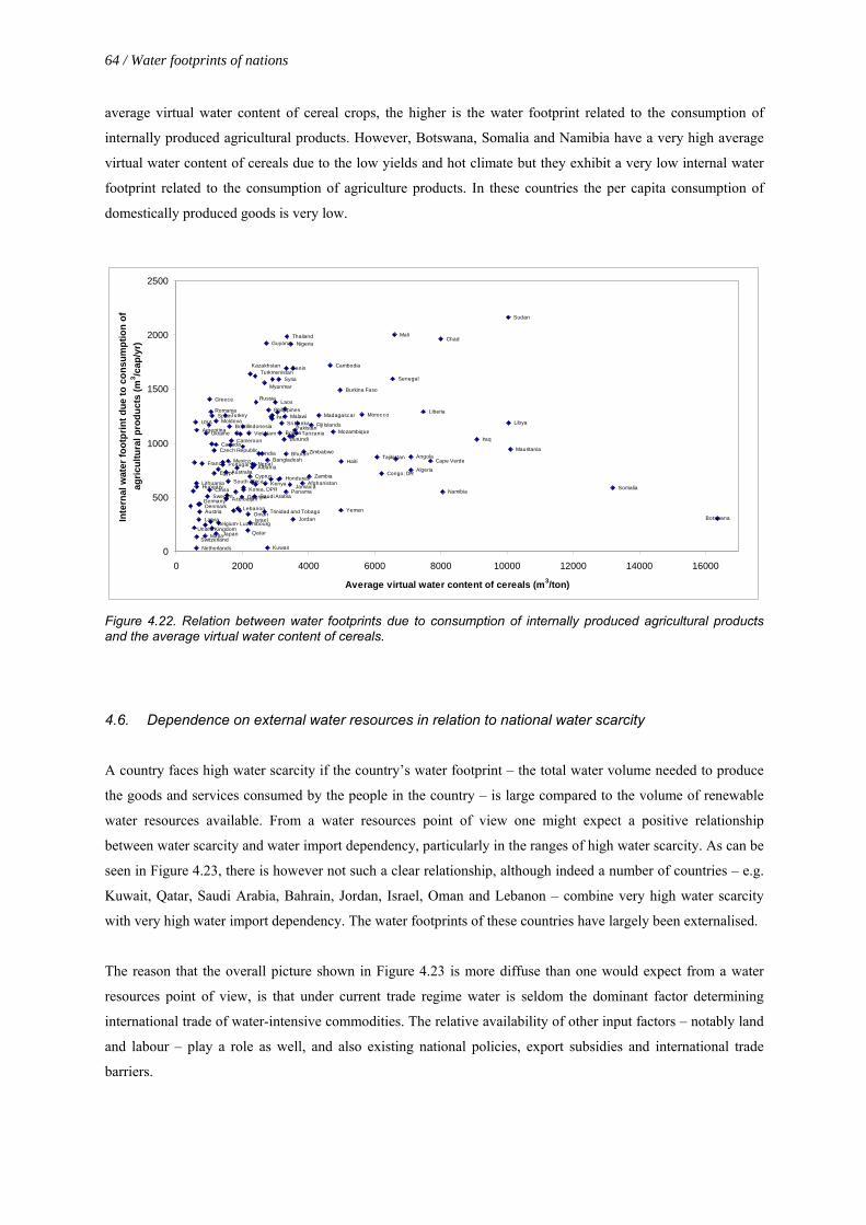
64 / Water footprints of nations a
average virtual water content of cereal crops, the higher is the water footprint related to the consumption of
internally produced agricultural products. However, Botswana, Somalia and Namibia have a very high average
virtual water content of cereals due to the low yields and hot climate but they exhibit a very low internal water
footprint related to the consumption of agriculture products. In these countries the per capita consumption of
domestically produced goods is very low.
United Kingdom
USA
Netherlands
Lithuania
Argentina
Hungary
Switzerland
Germany
LatviaAustriaDenmark
France
Malta
Ukraine
Sweden
Greece
China
RomaniaSpain
Belgium- Luxembourg
Czech Republic
Egypt
Moldova
Japan
Canada
Portugal
Turkey
Australia
Azerbaijan
Mexico
South Africa
Brazil
Cameroon
Lebanon
Georgia
Indonesia
Korea, DPR
Qatar
Oman
Viet Nam
Cyprus
Israel
Kazakhstan
NepalAlbania
Saudi Arabia
Turkmenistan
Russia
India
Trinidad and Tobago
Myanmar
Kenya
Guyana
Kuwait
Bangladesh
PhilippinesIran
Laos
Syria
Honduras
Bolivia
Sri Lanka
Burundi
Malawi
Panama
Bhutan
Benin
Thailand
Jamaica
Nigeria
Jordan
PakistanTanzania
Afghanistan
Zimbabwe
Zambia
Fiji Islands
Madagascar
Cambodia
Mozambique
Burkina Faso
Yemen
Haiti
Morocco
Tajikistan
Congo, DR
Senegal
Mali
Angola
Algeria
Liberia
Cape Verde
Chad
Namibia
Iraq
Sudan
Libya
Mauritania
Somalia
Botswana
0
500
1000
1500
2000
2500
0 2000 4000 6000 8000 10000 12000 14000 16000
Average virtual water content of cereals (m3/ton)
Inte
rnal
wat
er fo
otpr
int d
ue to
con
sum
ptio
n of
ag
ricul
tura
l pro
duct
s (m
3 /cap
/yr)
Figure 4.22. Relation between water footprints due to consumption of internally produced agricultural products and the average virtual water content of cereals.
4.6. Dependence on external water resources in relation to national water scarcity
A country faces high water scarcity if the country’s water footprint – the total water volume needed to produce
the goods and services consumed by the people in the country – is large compared to the volume of renewable
water resources available. From a water resources point of view one might expect a positive relationship
between water scarcity and water import dependency, particularly in the ranges of high water scarcity. As can be
seen in Figure 4.23, there is however not such a clear relationship, although indeed a number of countries – e.g.
Kuwait, Qatar, Saudi Arabia, Bahrain, Jordan, Israel, Oman and Lebanon – combine very high water scarcity
with very high water import dependency. The water footprints of these countries have largely been externalised.
The reason that the overall picture shown in Figure 4.23 is more diffuse than one would expect from a water
resources point of view, is that under current trade regime water is seldom the dominant factor determining
international trade of water-intensive commodities. The relative availability of other input factors – notably land
and labour – play a role as well, and also existing national policies, export subsidies and international trade
barriers.
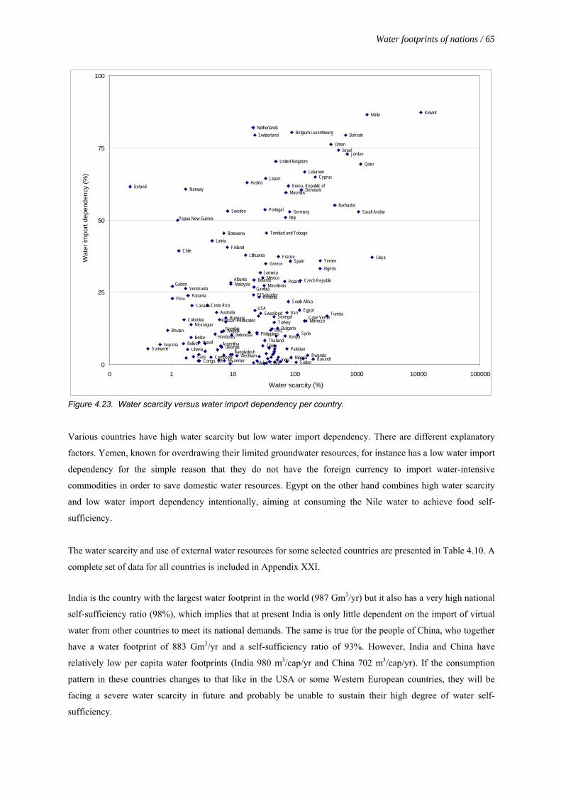
Water footprints of nations / 65
Kuwait
Libya
Malta
Qatar
Saudi Arabia
Jordan
Bahrain
Israel
Barbados
Oman
Tunisia
YemenAlgeria
Cyprus
BurundiRwanda
Morocco
Lebanon
Cape Verde
Denmark
Czech Republic
Egypt
Syria
Sudan
Belgium-Luxembourg
Nigeria
Spain
Germany
Korea, Republic of
South Africa
Iran
Pakistan
Mauritius
Italy
Kenya
Poland
France
Bulgaria
India
United Kingdom
TurkeySenegal
Iraq
Trinidad and Tobago
Chad
Japan
Greece
Portugal
Thailand
MauritaniaMexico
China
Swaziland
Jamaica
Armenia
Philippines
USA
Switzerland
Belarus
Hungary
Gambia
Mali
El Salvador
Netherlands
Austria
Lithuania
Viet NamBangladesh
Indonesia
MalaysiaAlbania
Sweden
Finland
Myanmar
Botswana
AngolaNamibia
GeorgiaArgentina
Russian FederationAustralia
Honduras
Latvia
Cambodia
Costa Rica
Congo, DR
Brazil
Laos
Canada
Belize
Nicaragua
Panama
Liberia
Norway
Venezuela
Colombia
Bolivia
Chile
Papua New Guinea
Gabon
Peru
Bhutan
GuyanaSuriname
Iceland
0
25
50
75
100
0 1 10 100 1000 10000 100000
Water scarcity (%)
Wat
er im
port
depe
nden
cy (%
)
Figure 4.23. Water scarcity versus water import dependency per country.
Various countries have high water scarcity but low water import dependency. There are different explanatory
factors. Yemen, known for overdrawing their limited groundwater resources, for instance has a low water import
dependency for the simple reason that they do not have the foreign currency to import water-intensive
commodities in order to save domestic water resources. Egypt on the other hand combines high water scarcity
and low water import dependency intentionally, aiming at consuming the Nile water to achieve food self-
sufficiency.
The water scarcity and use of external water resources for some selected countries are presented in Table 4.10. A
complete set of data for all countries is included in Appendix XXI.
India is the country with the largest water footprint in the world (987 Gm3/yr) but it also has a very high national
self-sufficiency ratio (98%), which implies that at present India is only little dependent on the import of virtual
water from other countries to meet its national demands. The same is true for the people of China, who together
have a water footprint of 883 Gm3/yr and a self-sufficiency ratio of 93%. However, India and China have
relatively low per capita water footprints (India 980 m3/cap/yr and China 702 m3/cap/yr). If the consumption
pattern in these countries changes to that like in the USA or some Western European countries, they will be
facing a severe water scarcity in future and probably be unable to sustain their high degree of water self-
sufficiency.
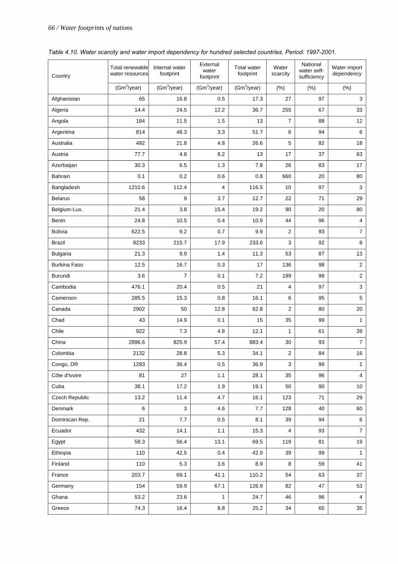
66 / Water footprints of nations a
Table 4.10. Water scarcity and water import dependency for hundred selected countries. Period: 1997-2001.
Total renewable water resources
Internal water footprint
External water
footprint
Total water footprint
Water scarcity
National water self-sufficiency
Water import dependency Country
(Gm3/year) (Gm3/year) (Gm3/year) (Gm3/year) (%) (%) (%)
Afghanistan 65 16.8 0.5 17.3 27 97 3
Algeria 14.4 24.5 12.2 36.7 255 67 33
Angola 184 11.5 1.5 13 7 88 12
Argentina 814 48.3 3.3 51.7 6 94 6
Australia 492 21.8 4.8 26.6 5 82 18
Austria 77.7 4.8 8.2 13 17 37 63
Azerbaijan 30.3 6.5 1.3 7.8 26 83 17
Bahrain 0.1 0.2 0.6 0.8 660 20 80
Bangladesh 1210.6 112.4 4 116.5 10 97 3
Belarus 58 9 3.7 12.7 22 71 29
Belgium-Lux. 21.4 3.8 15.4 19.2 90 20 80
Benin 24.8 10.5 0.4 10.9 44 96 4
Bolivia 622.5 9.2 0.7 9.9 2 93 7
Brazil 8233 215.7 17.9 233.6 3 92 8
Bulgaria 21.3 9.9 1.4 11.3 53 87 13
Burkina Faso 12.5 16.7 0.3 17 136 98 2
Burundi 3.6 7 0.1 7.2 199 98 2
Cambodia 476.1 20.4 0.5 21 4 97 3
Cameroon 285.5 15.3 0.8 16.1 6 95 5
Canada 2902 50 12.8 62.8 2 80 20
Chad 43 14.9 0.1 15 35 99 1
Chile 922 7.3 4.8 12.1 1 61 39
China 2896.6 825.9 57.4 883.4 30 93 7
Colombia 2132 28.8 5.3 34.1 2 84 16
Congo, DR 1283 36.4 0.5 36.9 3 99 1
Côte d'Ivoire 81 27 1.1 28.1 35 96 4
Cuba 38.1 17.2 1.9 19.1 50 90 10
Czech Republic 13.2 11.4 4.7 16.1 123 71 29
Denmark 6 3 4.6 7.7 128 40 60
Dominican Rep. 21 7.7 0.5 8.1 39 94 6
Ecuador 432 14.1 1.1 15.3 4 93 7
Egypt 58.3 56.4 13.1 69.5 119 81 19
Ethiopia 110 42.5 0.4 42.9 39 99 1
Finland 110 5.3 3.6 8.9 8 59 41
France 203.7 69.1 41.1 110.2 54 63 37
Germany 154 59.9 67.1 126.9 82 47 53
Ghana 53.2 23.6 1 24.7 46 96 4
Greece 74.3 16.4 8.8 25.2 34 65 35

Water footprints of nations / 67
Total renewable water resources
Internal water footprint
External water
footprint
Total water footprint
Water scarcity
National water self-sufficiency
Water import dependency
India 1896.7 971.4 16 987.4 52 98 2
Indonesia 2838 242.3 27.7 270 10 90 10
Iran 137.5 84.2 18.4 102.7 75 82 18
Iraq 75.4 27.2 3.7 30.9 41 88 12
Israel 1.7 2.2 6.4 8.6 514 26 74
Italy 191.3 65.9 68.7 134.6 70 49 51
Japan 430 51.9 94.2 146.1 34 36 64
Jordan 0.9 1.7 4.6 6.3 713 27 73
Kazakhstan 109.6 26.6 0.4 27 25 99 1
Kenya 30.2 19.1 2.1 21.2 70 90 10
Korea Rep. 69.7 21 34.2 55.2 79 38 62
Korea, DPR 77.1 16.7 2.1 18.8 24 89 11
Kuwait 0 0.3 1.9 2.2 10895 13 87
Kyrgyzstan 20.6 6.6 0 6.6 32 100 0
Lebanon 4.4 2.1 4.3 6.4 146 33 67
Libya 0.6 6.8 4 10.8 1793 63 37
Madagascar 337 19.5 0.3 19.8 6 98 2
Malawi 17.3 12.9 0.1 13 75 99 1
Malaysia 580 38.9 15 53.9 9 72 28
Mali 100 21.5 0.1 21.6 22 99 1
Malta 0.1 0.1 0.6 0.7 1478 13 87
Mexico 457.2 98 42.1 140.2 31 70 30
Morocco 29 37 6.6 43.6 150 85 15
Mozambique 216.1 19.4 0.1 19.5 9 100 0
Myanmar 1045.6 74.4 1.1 75.5 7 99 1
Nepal 210.2 18.7 0.7 19.3 9 96 4
Netherlands 91 3.5 15.9 19.4 21 18 82
Nigeria 286.2 242.2 5.9 248.1 87 98 2
Oman 1 0.9 2.9 3.8 389 24 76
Pakistan 222.7 157.3 8.9 166.2 75 95 5
Papua New Guinea 801 5.1 5.1 10.2 1 50 50
Paraguay 336 5.8 0.1 5.9 2 98 2
Peru 1913 15.4 4.6 20 1 77 23
Philippines 479 104.4 12.5 116.8 24 89 11
Poland 61.6 30.4 12.3 42.6 69 71 29
Portugal 68.7 10.5 12.1 22.6 33 46 54
Qatar 0.1 0.2 0.4 0.6 1176 31 69
Romania 211.9 34.6 4.3 38.9 18 89 11
Russia 4507.3 228.9 42.1 271 6 84 16
Rwanda 5.2 8.2 0.3 8.4 162 97 3
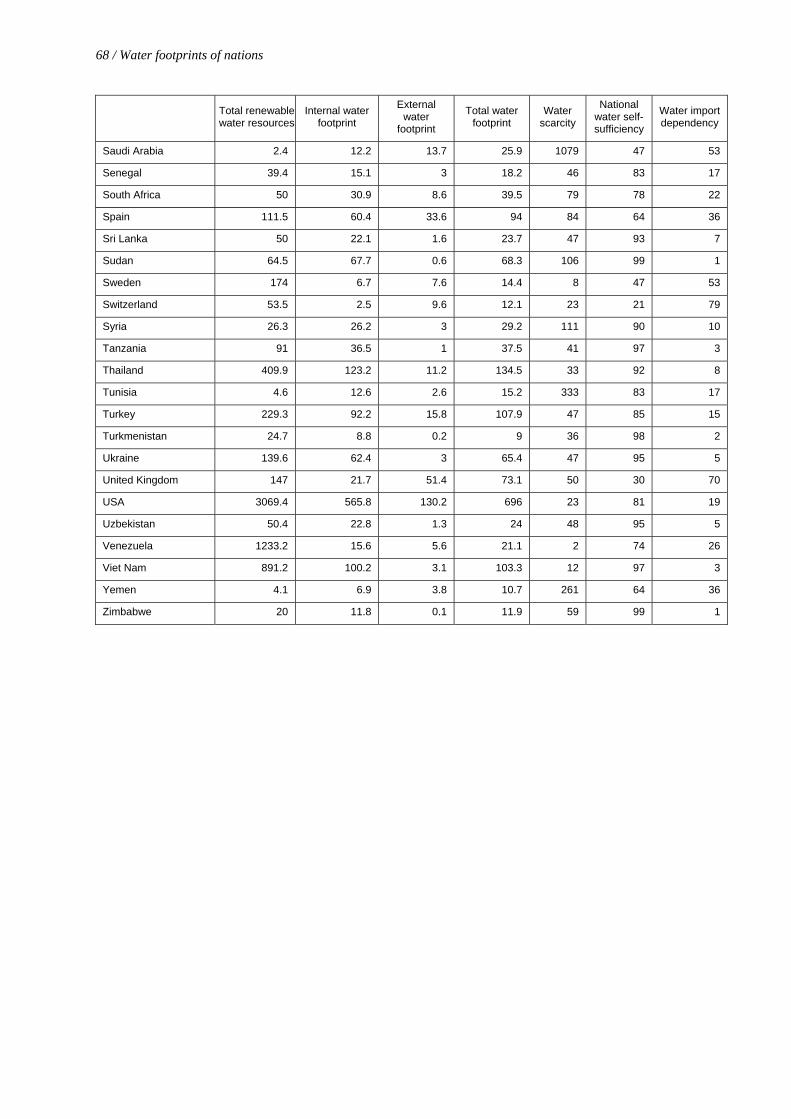
68 / Water footprints of nations a
Total renewable water resources
Internal water footprint
External water
footprint
Total water footprint
Water scarcity
National water self-sufficiency
Water import dependency
Saudi Arabia 2.4 12.2 13.7 25.9 1079 47 53
Senegal 39.4 15.1 3 18.2 46 83 17
South Africa 50 30.9 8.6 39.5 79 78 22
Spain 111.5 60.4 33.6 94 84 64 36
Sri Lanka 50 22.1 1.6 23.7 47 93 7
Sudan 64.5 67.7 0.6 68.3 106 99 1
Sweden 174 6.7 7.6 14.4 8 47 53
Switzerland 53.5 2.5 9.6 12.1 23 21 79
Syria 26.3 26.2 3 29.2 111 90 10
Tanzania 91 36.5 1 37.5 41 97 3
Thailand 409.9 123.2 11.2 134.5 33 92 8
Tunisia 4.6 12.6 2.6 15.2 333 83 17
Turkey 229.3 92.2 15.8 107.9 47 85 15
Turkmenistan 24.7 8.8 0.2 9 36 98 2
Ukraine 139.6 62.4 3 65.4 47 95 5
United Kingdom 147 21.7 51.4 73.1 50 30 70
USA 3069.4 565.8 130.2 696 23 81 19
Uzbekistan 50.4 22.8 1.3 24 48 95 5
Venezuela 1233.2 15.6 5.6 21.1 2 74 26
Viet Nam 891.2 100.2 3.1 103.3 12 97 3
Yemen 4.1 6.9 3.8 10.7 261 64 36
Zimbabwe 20 11.8 0.1 11.9 59 99 1
Water footprints of nations / 69
5. Conclusion
The global water footprint is 7450 Gm3/yr, which is 1240 m3/cap/yr. The differences between countries are
large: the USA has an average water footprint of 2480 m3/cap/yr whereas China has an average water footprint
of 700 m3/cap/yr. There are four most important factors explaining high water footprints. A first factor is the
total volume of consumption, which is generally related to gross national income of a country. This partially
explains the high water footprints of for instance the USA, Italy and Switzerland. A second factor behind a high
water footprint can be that people have a water-intensive consumption pattern. Particularly high consumption of
meat significantly contributes to a high water footprint. This factor partially explains the high water footprints of
countries such as the USA, Canada, France, Spain, Portugal, Italy and Greece. The average meat consumption in
the United States is for instance 120 kg/yr, more than three times the world-average meat consumption. Next to
meat consumption, high consumption of industrial goods significantly contributes to the total water footprints of
rich countries. The third factor is climate. In regions with a high evaporative demand, the water requirement per
unit of crop production is relatively large. This factor partially explains the high water footprints in countries
such as Senegal, Mali, Sudan, Chad, Nigeria and Syria. A fourth factor that can explain high water footprints is
water-inefficient agricultural practice, which means that water productivity in terms of output per drop of water
is relatively low. This factor partly explains the high water footprints of countries such as Thailand, Cambodia,
Turkmenistan, Sudan, Mali and Nigeria. In Thailand for instance, rice yields averaged 2.5 ton/ha in the period
1997-2001, while the global average in the same period was 3.9 ton/ha.
Reducing water footprints can be done in various ways. A first way is to break the seemingly obvious link
between economic growth and increased water use, for instance by adopting production techniques that require
less water per unit of product. Water productivity in agriculture can be improved for instance by applying
advanced techniques of rainwater harvesting and supplementary irrigation. A second way of reducing water
footprints is to shift to consumptions patterns that require less water, for instance by reducing meat consumption.
However, it has been debated whether this is a feasible road to go, since the world-wide trend has been that meat
consumption increases rather than decreases. Probably a broader and subtler approach will be needed, where
consumption patterns are influenced by pricing, awareness raising, labelling of products or introduction of other
incentives that make people change their consumption behaviour. Water costs are generally not well reflected in
the price of products due to the subsidies in the water sector. Besides, the general public is – although often
aware of energy requirements – hardly aware of the water requirements in producing their goods and services.
A third method that can be used – not yet broadly recognized as such – is to shift production from areas with low
water-productivity to areas with high water productivity, thus increasing global water use efficiency. For
instance, Jordan has successfully externalised its water footprint by importing wheat and rice products from the
USA, which has higher water productivity than Jordan.
The water footprint of a nation is an indicator of water use in relation to the consumption volume and pattern of
the people. As an aggregated indicator it shows the total water requirement of a nation, a rough measure of the
impact of human consumption on the natural water environment. More information about the precise
components and characteristics of the total water footprint will be needed, however, before one can make a more

70 / Water footprints of nations a
balanced assessment of the effects on the natural water systems. For instance, one has to look at what is blue
versus green water use, because use of blue water often affects the environment more than green water use. Also
it is relevant to consider the internal versus the external water footprint. Externalising the water footprint for
instance means externalising the environmental impacts. Also one has to realise that some parts of the total
water footprint concern use of water for which no alternative use is possible, while other parts relate to water
that could have been used for other purposes with higher added value. There is a difference for instance between
beef produced in extensively grazed grasslands of Botswana (use of green water without alternative use) and
beef produced in an industrial livestock farm in the Netherlands (partially fed with imported irrigated feed
crops).
International water dependencies are substantial and are likely to increase with continued global trade
liberalisation. Today, 16% of global water use is not for producing products for domestic consumption but for
making products for export. Considering this substantial percentage and the upward trend, we suggest that future
national and regional water policy studies should include an analysis of international or interregional virtual
water flows.
Virtual water can be regarded as an alternative source of water. Virtual water import can be used by national
governments as a tool to release the pressure on their domestic water resources. Jordan for instance annually
imports a virtual water volume that is more than five times its own annually renewable water resources.
Although saving their own domestic water resources, it increases Jordan’s dependency on other nations. Other
water-scarce countries such as Israel, Lebanon, Kuwait, Qatar, Bahrain, Oman and Malta have a similar high
water import dependency.
Global virtual water trade can effectively save water if products are traded from countries with high to countries
with low water productivity. For example, Mexico imports wheat, maize and sorghum from the USA (equivalent
to 7.1 Gm3/yr). If Mexico would produce the imported crops domestically, it would require 15.6 Gm3 of water
per year. Thus, from a global perspective, the trade of cereals from the USA to Mexico saves 8.5 Gm3/yr.
The current assessment of water footprints of nations carries a number of shortcomings, even though a number
of improvements have been carried through if compared to our earlier assessments (Hoekstra and Hung, 2002;
Chapagain and Hoekstra, 2003a). An important shortcoming is that the estimates of virtual water content of
crops are based on crop water requirements, which leads to overestimates in those cases where actual water
availability is lower than the crop water requirement. The calculations could be improved by using the actual
water use by crops as a basis, which however will require more specific data per crop per country (that we did
not have for the current study).
A matter for future consideration is the issue of including or excluding irrigation losses from the water footprint
definition. In the current study we have not included them mainly for the practical reason that data on irrigation
losses are generally not specified per crop, so that they cannot be included in the calculation of the virtual water
content of specific crops. But it can be argued that it is indeed right to exclude irrigation losses, because these
losses largely return to the system again. The counter-arguments in favour of including the losses are that the
Water footprints of nations / 71
withdrawal in itself has an impact already that should not be neglected (the return flows do not return to the
precise place where to were withdrawn), that a fraction of the total loss really gets lost for further use through
evaporation, and that return flows are often polluted and cannot be reused without treatment or dilution.
A second shortcoming in the current assessment of water footprints is that we have focused on expressing the
impact of human activities on the quantitative use of water resources. The water footprint concept has been
defined in this study as the quantity of water required to fulfil human’s demand for goods and services. Further
development of the water footprint concept would expand the water footprint definition in order to include
impacts of human activities on water quality as well.
Besides improvements, there is also room for refinements. The water footprint related to the consumption of
industrial products has been estimated for instance in a relatively quick and crude way, without specifically
looking at the specific water requirements for all kind of different industrial products. The methodology
currently applied yields results that suffice as overall estimates, but gives little product-specific information.
Finally, the challenge is to start using the water footprint concept as a practical tool to analyse how consumption
patterns affect water use, how future changes in consumption patterns are likely to impact on water, how
countries can externalise their water footprint in order to reduce the pressure on the domestic water resources
and how other countries can profit from their relative abundance of water by exporting water-rich commodities.


Water footprints of nations / 73
References Allan, J.A. (1993) ‘Fortunately there are substitutes for water otherwise our hydro-political futures would be
impossible’ In: Priorities for water resources allocation and management, ODA, London, pp. 13-26.
Allan, J.A. (1994) ‘Overall perspectives on countries and regions’ In: Rogers, P. and Lydon, P. Water in the
Arab World: perspectives and prognoses, Harvard University Press, Cambridge, Massachusetts, pp. 65-100.
Allen, R.G., Pereira, L.S., Raes, D., and Smith, M. (1998) ‘Crop evapotranspiration - Guidelines for computing
crop water requirements - FAO Irrigation and drainage paper 56’. Food and Agriculture Organization of the
United Nations, Rome, Italy. http://www.fao.org/docrep/X0490E/x0490e00.htm 1 April 2004.
Chapagain, A.K. and Hoekstra, A.Y. (2003a) ‘Virtual water flows between nations in relation to trade in
livestock and livestock products’, Value of Water Research Report Series No. 13, UNESCO-IHE, Delft, the
Netherlands. http://www.waterfootprint.org/Reports/Report13.pdf
Chapagain, A.K. and Hoekstra, A.Y. (2003b) ‘The water needed to have the Dutch drink coffee’, Value of Water
Research Report Series No. 14, UNESCO-IHE, Delft, the Netherlands.
http://www.waterfootprint.org/Reports/Report14.pdf
Chapagain, A.K. and Hoekstra, A.Y. (2003c) ‘The water needed to have the Dutch drink tea’, Value of Water
Research Report Series No. 15, UNESCO-IHE, Delft, the Netherlands.
http://www.waterfootprint.org/Reports/Report15.pdf
CIA (2004). ‘The World Fact Book’ USA. http://www.odci.gov/cia/publications/factbook/
FAO (2003a) ‘CROPWAT model’, Food and Agriculture Organization of the United Nations, Rome, Italy.
http://www.fao.org/ag/AGL/aglw/cropwat.htm
FAO (2003b) ‘CLIMWAT database’, Food and Agriculture Organization of the United Nations, Rome, Italy.
http://www.fao.org/ag/AGL/aglw/climwat.stm
FAO (2003c) ‘Thermal climate classification’, Food and Agriculture Organization of the United Nations, Rome,
Italy. http://www.fao.org/ag/AGL/agll/gaez/tab/t3.htm
FAO (2003d) ‘Review of global agricultural water use per country, irrigation water withdrawal’, Food and
Agriculture Organization of the United Nations, Rome, Italy.
http://www.fao.org/landandwater/aglw/aquastat/water_use/index5.stm

74 / Water footprints of nations a
FAO (2003e) ‘Review of global agricultural water use per country, crop water requirements’, Food and
Agriculture Organization of the United Nations, Rome, Italy.
http://www.fao.org/ag/agl/aglw/aquastat/water_use/index4.stm
FAO (2003f) ‘AQUASTAT 2002’, Food and Agriculture Organization of the United Nations, Rome, Italy.
ftp://ftp.fao.org/agl/aglw/aquastat/aquastat2002.xls.
FAO (2003g) ‘AQUASTAT 2003’, Food and Agriculture Organization of the United Nations, Rome, Italy.
ftp://ftp.fao.org/agl/aglw/aquastat/aquastat2003.xls.
FAO (2003h), ‘Technical Conversion Factors for Agricultural Commodities’, Food and Agriculture Organization
of the United Nations, Rome, Italy. http://www.fao.org/WAICENT/FAOINFO/ECONOMIC/ESS/pdf/tcf.pdf
FAO (2004) ‘Glossary of Land Water Terms’, Food and Agriculture Organization of the United Nations, Rome,
Italy. http://www.fao.org/landandwater/glossary/lwglos.jsp, 1 April 2004.
FAOSTAT (2004) ‘FAOSTAT on-line database’, Food and Agriculture Organization of the United Nations,
Rome, Italy. http://apps.fao.org/default.jsp. 15 February 2004.
Frederick S. Pardee Centre (2004) ‘The project on human development’ Boston University.
http://humandevelopment.bu.edu/
Haddadin, M.J. (2003) ‘Exogenous water: A conduit to globalization of water resources’. In: Hoekstra, A.Y.
‘Virtual water trade: Proceedings of the International Expert Meeting on Virtual Water Trade’, Value of Water
Research Report Series No. 12, UNESCO-IHE, Delft, the Netherlands.
http://www.waterfootprint.org/Reports/Report12.pdf
Hoekstra, A.Y. and Hung, P.Q. (2002) ‘Virtual water trade: A quantification of virtual water flows between
nations in relation to international crop trade’, Value of Water Research Report Series No. 11, UNESCO-IHE
Institute for Water Education, Delft, the Netherlands. http://www.waterfootprint.org/Reports/Report11.pdf
IMF (2004) ‘World Economic Outlook Database’, International Monetary Fund.
Mitchel, T. (2003) ‘TYN CY 1.1’, Tyndall Centre for Climate Change Research, Climatic Research Unit,
University of East Anglia, UK. http://www.cru.uea.ac.uk/~timm/cty/obs/TYN_CY_1_1.html. 21 August 2003.
Oki, T.; Sato, M.; Kawamura, A.; Miyake, M.; Kanae, S., and Musiake, K. (2003) 'Virtual water trade to Japan
and in the world'. In: Hoekstra, A.Y. ‘Virtual water trade: Proceedings of the International Expert Meeting on
Virtual Water Trade’, Value of Water Research Report Series No. 12, UNESCO-IHE, Delft, the Netherlands.
http://www.waterfootprint.org/Reports/Report12.pdf
Water footprints of nations / 75
PC-TAS (2000) ‘PC-TAS version 1995-99 in HS or SITC’, CD-ROM, United Nations Statistics Division, New
York, USA.
PC-TAS (2004) ‘PC-TAS version 1997-2001 in HS or SITC’, CD-ROM, United Nations Statistics Division,
New York, USA.
Raskin, P., Gleick, P., Kirshen, P., Pontius, G., and Strzepek, K. (1997) Water futures: Assessment of long-range
patterns and problems Comprehensive assessment of the freshwater resources of the world, Stockholm
Environment Institute, Stockholm, Sweden.
UNSD (2004a) ‘Commodity Trade Statistics (COMTRADE) on CD-ROM (1997-2001)’
http://unstats.un.org/unsd/trade/dataextract/datapctas.htm.
UNSD (2004b) National Accounts Main Aggregates, United Nations Statistical division.
http://unstats.un.org/unsd/snaama/resultsGDP.asp
Wackernagel, M. and Jonathan, L. (2001) Measuring sustainable development: Ecological footprints. Centre for
Sustainability Studies, Universidad Anahuac de Xalapa, Mexico.
Wackernagel, M., Onisto, L., Linares, A.C., Falfan, I.S.L., Garcia, J.M., Guerrero, I.S., and Guerrero, M.G.S.
(1997) Ecological footprints of nations: How much nature do they use? - How much nature do they have?
Centre for Sustainability Studies, Universidad Anahuac de Xalapa, Mexico.
Wackernagel, M. and Rees, W. (1996) ‘Our ecological footprint: Reducing human impact on the Earth’, New
Society Publishers, Gabriola Island, B.C., Canada.
World Bank (2004) ‘World Development Indicator Data-Query’, The World Bank Group.
http://devdata.worldbank.org/data-query/, 1 March 2004.
WTO (2004a) Statistical database.
http://stat.wto.org/StatisticalProgram/WSDBStatProgramHome.aspx?Language=E E
WTO (2004b) “WTO Statistical datasets-Technical notes” Geneva, Switzerland.
http://stat.wto.org/StatisticalProgram/WSDBStatProgramTechNotes.aspx?Language=E
Yang, H. and Zehnder, A.J.B. (2002) Water scarcity and food import: A case study for Southern Mediterranean
countries, World Development 30(8): 1413-1430.
Zimmer, D. and Renault, D. (2003) ‘Virtual water in food production and global trade: Review of
methodological issues and preliminary results’ In: Hoekstra, A.Y. ‘Virtual water trade: Proceedings of the
International Expert Meeting on Virtual Water Trade’, Value of Water Research Report Series No. 12,
UNESCO-IHE, Delft, the Netherlands. http://www.waterfootprint.org/Reports/Report12.pdf

76 / Water footprints of nations a

National Institute for Public Health and the Environment
UNESCO-IHEP.O. Box 30152601 DA DelftThe Netherlands
Website www.unesco-ihe.orgPhone +31 15 2151715


