
i
i
CRANFIED UNIVERSITY
XIAODONG LI
VISUAL NAVIGATION IN
UNMANNED AIR VEHICLES WITH
SIMULTANEOUS LOCATION AND
MAPPING (SLAM)
CRANFIELD DEFENCE AND SECURITY
PhD

Cranfield University
Cranfield Defence and Security
PhD Thesis
Academic Year 2013-2014
Xiaodong Li
Visual Navigation in Unmanned Air
Vehicles with SLAM
Supervisor: Dr Nabil Aouf
January 2014
© Cranfield University, 2014. All rights reserved. No part of this publication
may be reproduced without the written permission of the copyright holder.

Abstract
This thesis focuses on the theory and implementation of visual navigation
techniques for Autonomous Air Vehicles in outdoor environments. The target of this
study is to fuse and cooperatively develop an incremental map for multiple air vehicles
under the application of Simultaneous Location and Mapping (SLAM).
Without loss of generality, two unmanned air vehicles (UAVs) are investigated
for the generation of ground maps from current and a priori data. Each individual UAV
is equipped with inertial navigation systems and external sensitive elements which can
provide the possible mixture of visible, thermal infrared (IR) image sensors, with a
special emphasis on the stereo digital cameras. The corresponding stereopsis is able to
provide the crucial three-dimensional (3-D) measurements. Therefore, the visual aerial
navigation problems tacked here are interpreted as stereo vision based SLAM (vSLAM)
for both single and multiple UAVs applications.
To begin with, the investigation is devoted to the methodologies of feature
extraction. Potential landmarks are selected from airborne camera images as distinctive
points identified in the images are the prerequisite for the rest.
Feasible feature extraction algorithms have large influence over feature
matching/association in 3-D mapping. To this end, effective variants of scale-invariant
feature transform (SIFT) algorithms are employed to conduct comprehensive
experiments on feature extraction for both visible and infrared aerial images.
As the UAV is quite often in an uncertain location within complex and cluttered
environments, dense and blurred images are practically inevitable. Thus, it becomes a
challenge to find feature correspondences, which involves feature matching between 1st
and 2nd
image in the same frame, and data association of mapped landmarks and camera
measurements. A number of tests with different techniques are conducted by
incorporating the idea of graph theory and graph matching. The novel approaches,
which could be tagged as classification and hypergraph transformation (HGTM) based
respectively, have been proposed to solve the data association in stereo vision based
navigation. These strategies are then utilised and investigated for UAV application
within SLAM so as to achieve robust matching/association in highly cluttered
environments.
The unknown nonlinearities in the system model, including noise would introduce
undesirable INS drift and errors. Therefore, appropriate appraisals on the pros and cons
of various potential data filtering algorithms to resolve this issue are undertaken in order
to meet the specific requirements of the applications. These filters within visual SLAM
were put under investigation for data filtering and fusion of both single and cooperative
navigation. Hence updated information required for construction and maintenance of a
globally consistent map can be provided by using a suitable algorithm with the
compromise between computational accuracy and intensity imposed by the increasing
map size. The research provides an overview of the feasible filters, such as extended
Kalman Filter, extended Information Filter, unscented Kalman Filter and unscented H
Infinity Filter.
As visual intuition always plays an important role for humans to recognise objects,
research on 3-D mapping in textures is conducted in order to fulfil the purpose of both
statistical and visual analysis for aerial navigation. Various techniques are proposed to
smooth texture and minimise mosaicing errors during the reconstruction of 3-D textured
maps with vSLAM for UAVs.
Finally, with covariance intersection (CI) techniques adopted on multiple sensors,
various cooperative and data fusion strategies are introduced for the distributed and
decentralised UAVs for Cooperative vSLAM (C-vSLAM). Together with the complex
structure of high nonlinear system models that reside in cooperative platforms, the
robustness and accuracy of the estimations in collaborative mapping and location are
achieved through HGTM association and communication strategies. Data fusion among
UAVs and estimation for visual navigation via SLAM were impressively verified and
validated in conditions of both simulation and real data sets.

Acknowledgments
This work was benefitted greatly from the support of many people over the past
years, and it is not possible to list everyone here. My gratitude at this completion is
extended especially to those mentioned below.
First of all, I would like to give thanks to my supervisor Dr Nabil Aouf. Thanks to
you for giving me this research opportunity, your availability, your expertise and
advice. To Professor Mark Richardson, my thesis committee member, thanks for your
motivation and encouragement. Special thanks for your reviews of this thesis, helpful
comments and wise counsel.
I really appreciated the help from Dr Fei, Dr Cheng, Dr Luke, Miss Ann, David
and good team mate Saad, Tarek and Dr Greer.
The team members of this unmanned Autonomous System Laboratory have made
my time enjoyable and rewarding, and have often provided a welcome respite from
research. Their names are Lounis, Karim, Steven, Redouane, Diego, Mohammed, Riad,
Oualid, Abdenour, Saif, Ivan, Luke.
I would like also to acknowledge and thank all the staff at the Defence Academy,
especially to Library and Learning Services.
My most valuable support by far has come from my family. Thank you, Min, for
your constant support and understanding.
Finally, I would like to thank all the people who have contributed to the
achievement of this work.
Shrivenham, 13th
January 2014 Xiaodong Li
i
Contents
CHAPTER 1 __________________________________________________________1
Introduction __________________________________________________________1 1.1 PhD Challenges ______________________________________________________________ 2 1.2 Research Motivation __________________________________________________________ 6 1.3 Thesis overview and Contribution ________________________________________________ 7
1.4 Publications _________________________________________________________________ 9
CHAPTER 2 _________________________________________________________11
SLAM Problem in General _____________________________________________11
2.1 Overview _____________________________________________________________ 12 2.1.1 SLAM in Robotics Navigation ________________________________________________ 12 2.1.2 Unscrambling Mapping and Localisation in SLAM ________________________________ 13 2.1.3 Data Fusion in SLAM _______________________________________________________ 14 2.1.4 Data Association in SLAM ___________________________________________________ 15
2.2 Overall Process of SLAM/vSLAM in Aerial Vehicles ________________________ 17
2.3 Technical Challenges in SLAM __________________________________________ 19
2.4 State of Art on the Specific Vision based SLAM _____________________________ 22
2.5 Cooperative SLAM ____________________________________________________ 25
2.6 Summary and Conclusion _______________________________________________ 30
CHAPTER 3 _________________________________________________________31
Camera Imaging, Modelling and Vision Processing _________________________31
3.1 Introduction __________________________________________________________ 31
3.2 Camera Imaging and Modelling __________________________________________ 32 3.2.1 Camera Image Formation ____________________________________________________ 32 3.2.2 Pinhole Camera Model – Perspective Model _____________________________________ 33 3.2.3 General Camera Matrix and Calibration _________________________________________ 36
3.3 Epipolar Geometry ____________________________________________________ 38 3.3.1 Introducing Epipolar Geometry _______________________________________________ 38 3.3.2 Stereo Camera Calibration ___________________________________________________ 42
3.4 Camera Imaging based Vision Processing __________________________________ 44 3.4.1 SIFT-Scale Invariance Feature Transform _______________________________________ 45 3.4.2 Affine-SIFT ______________________________________________________________ 47 3.4.3. Variants SIFT in VLFeat ____________________________________________________ 48 3.4.3.1 VL_SIFT ______________________________________________________________ 48 3.4.3.2 VL_DSIFT _____________________________________________________________ 48 3.4.3.3 VL_PHOW(Pyramid Histogram of Visual Words) ______________________________ 49
3.4.4 SURF-Speed Up Robust Features ______________________________________________ 50 3.4.5 Feature Matching and RANSAC Outlier Removal _________________________________ 52
3.5 Vision Processing in SLAM______________________________________________ 54
ii
3.6 Investigation on SIFT Features in Visible and Infrared Images ________________ 55 3.6.1. Experiment Requirements and Parameter Settings ________________________________ 55
3.6.2 Initial Tests _______________________________________________________________ 56 3.6.2.1 Sample Images __________________________________________________________ 56 3.6.2.2 Matching with RANSAC __________________________________________________ 56 3.6.2.3 Matching Comparision in Various Threshold __________________________________ 58
3.6.3 Feature Extraction/Matching cross Imaging Bands ________________________________ 59 3.6.4 Comprehensive Tests on Images in Different Environment __________________________ 62 3.6.5 Test for Feature Invariance ___________________________________________________ 65
3.7 Summary and Discussion _______________________________________________ 70
CHAPTER 4 _________________________________________________________72
Data Filtering and Estimation Analysis in vSLAM _________________________72
4.1 Introduction ______________________________________________________72
4.2 Extended Kalman Filter_____________________________________________76
4.3 Unscented Kalman Filter ____________________________________________77
4.3.1 Unscented Transform(UT) Technique ___________________________________ 77
4.3.2 Unscented Kalman Filter(UKF) ________________________________________ 79
4.3.3 Advantage of Unscented Kalman Filter __________________________________ 80
4.4 Unscented H Infinity Filter __________________________________________80
4.4.1 Advantage of Unscented H Filter ______________________________________ 82
4.5 Extended Informatin Filter(EIF) _____________________________________83
4.5.1 Advantage of Informatin Filter _________________________________________ 84
4.6 System Models in Aerial vSLAM _____________________________________85
4.6.1 Introduction _________________________________________________________ 85
4.6.2 Process Model _______________________________________________________ 85
4.6.3 Observation Model ___________________________________________________ 86 4.6.3.1 3D Coodinates in Camera Model _____________________________________________ 87 4.6.3.2 Airborne Stereo Vision-Observation Model ____________________________________ 90 4.6.3.3 The State Structure of UAV vSLAM __________________________________________ 91
4.7 Experimental Study ________________________________________________92
4.7.1 Experiment Setup ____________________________________________________ 92
4.7.2 Filters test with SIFT _________________________________________________ 93
4.7.3 Filters test with SURF ________________________________________________ 94
4.8 Summary and Discussion ____________________________________________96
CHAPTER 5 _________________________________________________________98
3D Reconstruction with Textured Mapping in vSLAM ______________________98
5.1 Introduction __________________________________________________________ 98
5.2 3D Reconstruciton Pipeline Process ______________________________________ 100

iii
5.3 Homogeneous Coordinates and Homography ______________________________ 103
5.4 3D Texured Mapping __________________________________________________ 105 5.4.1 3D Surface Meshing _______________________________________________________ 105 5.4.2 Textured Mapping _________________________________________________________ 108
5.5 Image Mosaicing _____________________________________________________ 110 5.5.1 Technique Overview _______________________________________________________ 111 5.5.2 Homography Transformation in Image Registration ______________________________ 112
5.5.3 Mosaicing Compositing ____________________________________________________ 114 5.5.4 Mosaic Imaging __________________________________________________________ 115
5.6 Textured 3D Reconstruction with vSLAM ________________________________ 118 5.6.1 Textured Mapping Pipeline in vSLAM _________________________________________ 118 5.6.2 Synchronised Textured Mapping within vSLAM _________________________________ 120 5.6.3 Textured Mapping Based on Mosaic Imaging ___________________________________ 123
5.6.3.1 3D Reconstruction Textured with Mosaic Imaging _____________________________ 123
5.7 Summary and Conclusion ______________________________________________ 125
CHAPTER 6 ________________________________________________________127
Feature Matching and Association in Airborne Binocular vSLAM ___________127
6.1 Overview of Image Feature Matching and Association in vSLAM _____________ 127
6.2 Basic Notation and Terminology in Graph Theory _________________________ 129 6.2.1 Graph Concept ___________________________________________________________ 129 6.2.2 Graph Representation ______________________________________________________ 131 6.2.3 Dominating Set Concept ____________________________________________________ 131 6.2.4 Tests on Finding Dominating Set in Camera Image _______________________________ 132
6.3 Graph Matching ______________________________________________________ 134 6.3.1 Graph Matching Concept ___________________________________________________ 134
6.3.2 Emprical Investigation on Graph Matching _____________________________________ 136
6.3.3 Proposed Graph Matching __________________________________________________ 136 6.3.4 Graph Transformation ______________________________________________________ 136 6.3.5 Various Tests on Graph Based Feature Matching _________________________________ 138 6.3.6 Use of Graph Theory in vSLAM _____________________________________________ 141
6.4 Novel Proposals of Data Association Schema ______________________________ 144 6.4.1 Classification Based Data Association Strategy __________________________________ 145 6.4.2 Graph Based Data Association Strategy ________________________________________ 148
6.5 Summary and Discussion ______________________________________________ 151
CHAPTER 7 ________________________________________________________152
Collaborative Navigation of UAVs with vSLAM __________________________152
7.1 Overview ____________________________________________________________ 152
7.2 Covariance Intersection(CI) ____________________________________________ 154
7.3 Decentralised Cooperative Aerial vSLAM ________________________________ 156 7.3.1 State Structure in C-vSLAM _________________________________________________ 156 7.3.2 Experimental Results in Simulation ___________________________________________ 157
7.4 Experiments Conducted for C-vSLAM with Real Data Sets __________________ 161 7.4.1 Environment Configuration _________________________________________________ 162
7.4.2 Experimental Implementation ________________________________________________ 164

iv
7.4.3 Wideband Communication Model ____________________________________________ 166 7.4.4 Narrowband Communication Model ___________________________________________ 169
7.5 Summary and Discussion ______________________________________________ 172
CHAPTER 8 ________________________________________________________174
Conclusions and Future work __________________________________________174
References __________________________________________________________177
Time (s)
X p
ositio
n (
m)
True position
INS position
DC-VSLAM position

v
List of Figures
Figure 2.2.1 Overview Process of SLAM for UAV ....................................................... 19
Figure 2.4.1 General structure of visual SLAM workflow ............................................ 24
Figure 2.5.1 Distributed Centralised Multi-Platform ..................................................... 28
Figure 2.5.2 Distributed Decentralised Multi-Platform.................................................. 29
Figure 3.2.1 Camera coordinates, Image plane and Perspective Projection ................... 34
Figure 3.3.1 Epipolar Geometry ..................................................................................... 39
Figure 3.3.2 Pencils of Epipolar Lines ........................................................................... 39
Figure 3.6.1 EO images .................................................................................................. 56
Figure 3.6.2 IR iamges ................................................................................................... 56
Figure 3.6.3 EO images .................................................................................................. 56
Figure 3.6.4 IR images ................................................................................................... 56
Figure 3.6.5 Features matching with SIFT for EO images ............................................. 57
Figure 3.6.6 Features matching with SIFT for IR images .............................................. 57
Figure 3.6.7 Features matching with SURF for EO images ........................................... 57
Figure 3.6.8 Features matching with SURF for IR images ............................................ 57
Figure 3.6.9 EO tracking images .................................................................................... 59
Figure 3.6.10 IR tracking imgaes ................................................................................... 59
Figure 3.6.11 Visible and Corresponding Infrared images ............................................ 62
Figure 3.6.12 Visible images taken from MBDA TV with re-sample rates 0.2s ........... 66
Figure 3.6.13 Infrared images taken from MBDA TV with re-sample rates 0.2s .......... 66
Figure 3.6.14 Matched Features from visible images with 0.2s sampe rate................... 68
Figure 3.6.15 Matched Features from infrared images with 0.2s sampe rate................. 68
Figure 3.6.16a Matching rates (MR)(to 1st image) for EO images with 0.2s sampe
rate(without RANSAC) .................................................................................................. 68
Figure 3.6.17a Matching rates (MR)(to 1st image) for IR images with 0.2s sampe
rate(without RANSAC) .................................................................................................. 68
Figure 3.6.16b Matching rates (MR)(to 2nd
image) for EO images with 0.2s sampe
rate(without RANSAC) .................................................................................................. 69
Figure 3.6.17b Matching rates (MR)(to 2nd
image) for IR images with 0.2s sampe
rate(without RANSAC) .................................................................................................. 69
Figure 3.6.18a Matching rates (MR)(to 1st image) for EO images with 0.2s sampe
rate(with RANSAC) ....................................................................................................... 69
Figure 3.6.18b Matching rates (MR)(to 2nd
image) for EO images with 0.2s sampe
rate(with RANSAC) ....................................................................................................... 69
Figure 3.6.19a Matching rates (MR)(to 1st image) for IR images with 0.2s sampe
rate(with RANSAC) ....................................................................................................... 69
Figure 3.6.19b Matching rates (MR)(to 2nd
image) for IR images with 0.2s sampe
rate(with RANSAC) ....................................................................................................... 69
Figure 4.6.1 Camera model ............................................................................................ 87
Figure 4.6.2 Triangulation principle in 3D estimation ................................................... 88
Figure 4.6.3 Perspective camera model .......................................................................... 89
Figure 4.7.1 UAV used in the tests ................................................................................. 92
Figure 5.2.1 Process of 3D Reconstruction .................................................................. 102

vi
Figure 5.4.1 Delaunay Triangulation (DT) and messing grid by DT ........................... 107
Figure 5.4.2 Delaunay Triangulation (DT), Maximises smallest angles ..................... 107
Figure 5.4.3 Voronoi diagram (black) formulated based on DT (red) ......................... 107
Figure 5.4.4a Projective transformation of triangular section in concept ................... 109
Figure 5.4.4b Projective transformation of triangular section in real image ................ 109
Figure 5.4.5 Texture Plating on 3D Triangle surface .................................................. 109
Figure 5.5.1 Image mosaic flowchar based on SIFT/SURF ......................................... 114
Figure 5.5.2 Mosaicing ground images (top) in two frames with results (bottom) ...... 116
Figure 5.5.3a Example airborne images ....................................................................... 116
Figure 5.5.3b Mosaicing with airborne images in 2 frames ......................................... 116
Figure 5.5.3c Mosaicing with airborne images in 4 frames ......................................... 117
Figure 5.5.3d Mosaicing with airborne images in 10 frames ....................................... 117
Figure 5.5.3e Mosaicing with airborne images in 30 frames ....................................... 117
Figure 5.5.3f Mosaicing with airborne images in 100 frames ..................................... 117
Figure 5.6.1 Texture Mapping in vSLAM ................................................................... 119
Figure 5.6.2 3D clound points construction under real scene in vSLAM .................... 121
Figure 5.6.3 Texture 3D mapping in vSLAM with SIFT ........................................... 121
Figure 5.6.4 Texture 3D mapping in vSLAM with SURF .......................................... 122
Figure 5.6.5 Texture 3D mapping in vSLAM with SIFT without extra features ....... 122
Figure 5.6.6a Mosaicing image in 30 frames (images) ............................................... 124
Figure 5.6.6b 3D texture mapping on mosaic imaging in 2 frames ............................ 125
Figure 5.6.6c 3D texture mapping on mosaic imaging with SIFT .............................. 125
Figure 6.2.1 Hypergraph representation ....................................................................... 130
Figure 6.2.2 LHS: (1) the network graph, RHS: (2) the dominating set ...................... 132
Figure 6.2.3 CDS based on the features from aerial image .......................................... 134
Figure 6.3.1 GTM based feature matching on highly blurred aerial images ................ 138
Figure 6.3.2 Dominating data sets and graph matching in stereo images .................... 139
Figure 6.3.3 CDS+ GTM based feature matching on highly blurred aerial images ..... 140
Figure 6.3.4 NN principle based feature matching on highly blurred aerial images .... 140
Figure 6.3.5 NN+GTM based feature matching on highly blurred aerial images ........ 141
Figure 6.3.6 NN+RANSAC based feature matching on highly blurred aerial images 141
Figure 6.3.7a vSLAM with conventional matching strategy........................................ 142
Figure 6.3.7b vSLAM with CDS in matching strategy ................................................ 143
Figure 6.3.7c vSLAM with GTM in matching strategy ............................................... 144
Figure 6.4.1Classification based data association ........................................................ 146
Figure 6.4.1a Estimation of vSLAM with conventional association methods ............. 147
Figure 6.4.1b Estimation of vSLAM with proposed association strategy .................... 148
Figure 6.4.2 HGTM based data association ................................................................. 149
Figure 6.4.2a Estimation of vSLAM with conventional association methods ............. 150
Figure 6.4.2b Estimation of vSLAM with proposed GTM association strategy .......... 151
Figure 7.3.1a C-vSLAM trajectory............................................................................... 158
Figure 7.3.1b Error comparison of C-vSLAM and single vSLAM .............................. 159
Figure 7.3.1c Corresponding 2σ points of covariance 3D distribution for UAV1 ....... 159
Figure 7.3.1d Corresponding 2σ points of covariance 3D distribution for UAV2 ....... 159
Figure 7.3.2a C-vSLAM trajectory............................................................................... 160
Figure 7.3.2b Error comparison of C-vSLAM and single vSLAM .............................. 160

vii
Figure 7.3.2c Corresponding 2σ points of covariance 3D distribution for UAV1 ....... 160
Figure 7.3.2d Corresponding 2σ points of covariance 3D distribution for UAV2 ....... 161
Figure 7.4.1 UAV used in experiment .......................................................................... 162
Figure 7.4.1a Fight path and UAV configuration ......................................................... 163
Figure 7.4.1b Flight trajectory and Sectioned trajectory .............................................. 163
Figure 7.4.1c Example of stereo image pair taken on scene ........................................ 164
Figure 7.4.2a The validation of CI based data fusion for proposed C-SLAM model
(Conventional data association) under wideband network(UAV1) ............................. 166
Figure 7.4.2b The validation of CI based data fusion for proposed C-SLAM model
(Conventional data association) under wideband network(UAV2) ............................ 167
Figure 7.4.3a The validation of CI based data fusion for general C-SLAM model
(HGTM based data association) under wideband network(UAV1) ............................. 168
Figure 7.4.3b The validation of CI based data fusion for general C-SLAM model
(HGTM based data association) under wideband network(UAV2) ............................. 169
Figure 7.4.4a The validation of CI based data fusion for proposed C-SLAM model
(Conventional data association) under narrowband network(UAV1) ......................... 170
Figure 7.4.4b The validation of CI based data fusion for proposed C-SLAM model
(Conventional data association) under narrowband network(UAV2) .......................... 170
Figure 7.4.5a The validation of CI based data fusion for general C-SLAM model
(HGTM based data association) under narrowband network(UAV1).......................... 171
Figure 7.4.5b The validation of CI based data fusion for general C-SLAM model
(HGTM based data association) under narrowband network(UAV2).......................... 172
List of Tables
Table 3.6.1 Matching threshold based comparsion in SIFT and SURF ......................... 58
Table 3.6.2 Comparison for Feature Extraction and Matching cross Imaging Bands.... 59
Table.3.6.3 Feature Extraction and Matching from images in different Environments . 62
Table 3.6.4 Overview of Invariance comparision for Feature Extraction and Matching
from Visible and Infrared Images ................................................................................... 66
Table 4.7.1 RERs (SLAM-INS) of Filters with SIFT applied........................................ 94
Table 4.7.2 RERs (SLAM-INS) of Filters with SURF applied ...................................... 95
Table 7.4.1 Intrinsic parameters configured in the experiment .................................... 164
Table 7.4.2 Extrinsic parameters configured in the experiment ................................... 164

Nomenclature
xiv
xiv
Nomenclature
Roman symbols
azayax ,, IMU acceleration
rqp ,, IMU angular rates
ZYX ,, UAV position in navigation frame
WVU ,, UAV velocity in body frame
bnC Direct cosine transform matrix that rotates a vector from body frame
to the navigation frame
kP Variance covariance matrix
kkx /ˆ Estimated state at time step k
1/ˆ
kkx Predicted state
kw Process noise
kv Observation noise
kQ Process noise covariance matrix
kR Observation noise covariance matrix
ky Observation
(·, ·, ·) f Continuous Process model
(·, ·, ·)h Continuous Observation model
kK Kalman Gain
k Scale factor for image pyramid
I Original image
f Focal length
b Baseline
),( ll vu Feature coordinate in left image
),( rr vu Feature coordinate in right image
H Homography matrix
bin Orientation sampling

Nomenclature
xv
1cI , 2cI Intrinsic parameters of camera 1 and 2 respectively
vk Horizontal scale factor
uk Vertical scale factor
),( 00 vu Coordinate of optical centre
n
bC Rotation matrix from body to navigation frame
b
sC Rotation matrix from IMU to body frame
1
s
cC (2
s
cC ) Rotation matrix from the right (left) camera to the IMU frame
Greek symbols
,, UAV orientation in navigation frame
Jacobean
i High order term in Taylor development
H infinity bound
i Bounds of high order terms in Taylor development
Image scale
Acronyms
ASIFT Affine SIFT
CI Covariance intersection
CCD Charge-Coupled Device
CL Cooperative Localisation
CMOS Complementary Metal–Oxide–Semiconductor
C/S Client/Server
C-vSLAM Cooperative visual SLAM
DistRatio Distance ratio
DoD Department of Defence
DoF Degree of Freedom
DoG Difference of Gaussian
DT Delauney Triangulation
EKF Extended Kalman Filter

Nomenclature
xvi
EO Electro Optical
HD Horizontal Disparity
HGTM Hyper Graph Transformation Matching
HOG Histogram Of Gaussian
HSV Hue, Saturation, Value
HVS Human Vision System
IF Information Filter
IMU Inertial Measurement Unit
IR Infra-Red
INS Inertial Measurement System
GNSS Global Navigation Satellite System
GPS Global Positioning System
GTM Graph Transformation Matching
GRV Gaussian Random Variable
KF Kalman Filter
LoG Laplacian of Gaussian
MMSE Minimum Mean Square Error
NED North East Down
NH Nonlinear H
NN Nearest Neighbour
pdf Probalility distribution function
P2P Peer to Peer
RGB Red, Green, Blue
SIFT Scale Invariant Feature Transform
SURF Speeded Up Robust Features
SLAM Simultaneous Localisation And Mapping
S-SLAM Single Simultaneous Localisation And Mapping
SVD Singular Value Decomposition
S-vSLAM Single Visual Simultaneous Localisation And Mapping
UAV Unmanned Aerial Vehicle

Nomenclature
xvii
UAV1 Unmanned Aerial Vehicle 1
UAV2 Unmanned Aerial Vehicle 2
UKF Unscented Kalman Filter
UHF Unscented H infinity Filter
UT Unscented Transform
v(V)SLAM Visual Simultaneous Localisation And Mapping
VL Vision Library
VL_DSIFT Vision Library Dense SIFT
VL_PHOW Vision Library_ Pyramid Histogram of Visual Words
VL_SIFT Vision Library SIFT

Chapter 1 Introduction
1
CHAPTER 1
Introduction
In the fields of robotics, navigation is the process of determining locations of the
robot travelling safely from a starting point to its destination. To fulfil this purpose,
different sensors are normally employed so that a varied spectrum of solutions could be
obtained. Over the last decades, a lot of effort has been devoted to visual navigation for
mobile robots and numerous contributions have been made by many researchers [1-3,5-
12]. Since an autonomous mobile vehicle has to construct a map of the surrounding
environment and simultaneously track its own motion through the map for navigation,
vision based navigation strategies could significantly broaden the scope of the
application.
Many solutions to the intricate problem of autonomous navigation have been
proposed. Simultaneous localisation and mapping (SLAM) also known as Concurrent
Mapping and Localisation (CML) [1-3], which intends to build a map of an unknown
environment while simultaneously determining the location of the robot within this
map, is continually drawing considerable attention to the robotics community.
Traditionally, vision-based navigation solutions have mostly been devised for
Autonomous Ground Vehicles (AGV). In recent years, the higher mobility and
manoeuvrability of Unmanned Air Vehicles (UAVs) has attracted significant interest in
many fields of military and civilian sectors. On such occasions, UAVs offer great
perspectives in missions like surveillance, patrolling, search and rescue, outdoor and
indoor building inspection, where there are considerable shortcomings for ground robots
due to their limited ability to access.
Besides, the typical solution of SLAM with sensing facilities like range-bearing
radar, laser or certain brands of sonar, may not be feasible with a UAV. This is due to
the reduced size of the UAV which limits its payload capabilities so that it is unable to
carry such sensors available for ground vehicles. In contrast, low cost, light weight
digital cameras which provide an information enriched perception of the environment in

Chapter 1 Introduction
2
a single shot become very competitive in visual navigation of vehicles. These merits
have given vision systems growing importance in mobile robotics during the last years.
In vSLAM (SLAM with vision sensing - vSLAM), vision-based processing
methods drawn from computer vision play an important role. They provide
measurements through features extraction from the observations of environment to
achieve simultaneous mapping and localising. This makes vSLAM approach highly
dependent on the available visual information.
However, the image resolution could be restricted due to the flight of UAVs with
vibration at condition of high altitudes. Moreover, the inherent errors in the image
formation and in the detection of features can further increase uncertainty in the
observed landmarks or other objects of interest. All these issues introduce many
challenges to this research.
Initially, SLAM methods were developed for a single vehicle. However, in reality,
the complexity of some applications requires cooperation among several robots. This
imposes multiple vehicles or multi-sensors collaborative SLAM (C-SLAM) [7, 8]. It is
also understood that the use of multiple co-operating vehicles for missions (e.g.
mapping or exploration) has many advantages over single-vehicle architecture. The
main contribution is the enhancement of estimation accuracy given by optimised
weights obtained from fusing algorithms [7, 8].
These practical requirements mark the key motivation for this research, which
aims to have multiple unmanned air vehicles with their own sensors and navigation
systems, to collaboratively generate a navigating map. Their utilisation is based on their
robust and flexible perception system that can provide broad visual environmental
information for navigation. In addition, the available sensors and systems may not need
to be identical. The architecture of the sensors system allows both single-UAV and
cooperating UAVs perception to be fulfilled. It considers, within the scope of this
research, infrared and visual cameras. However, it can later be adapted to other sensors.
1.1 PhD Challenges
In this research, the main concerns focus on the investigation and implementation
of navigation with visual SLAM to enable multiple UAVs operating in their
Chapter 1 Introduction
3
environments to collaborate without external intervention. There is doomed to have
more difficulties encountered when utilising navigation and guidance algorithms for the
air vehicle’ autonomy in the aerial environment, where the sensing operation is
conducted for obtaining information through measurement to meet the requirement of
self-localisation and map building. This is supposed to occur in the 6 DoF vibration of a
vehicle, where erratic motion and rough terrain tend to generate image features which
are more blurred and less distinctive. In this case, the development of a feasible and
reliable airborne cooperative visual SLAM system on the decentralised cooperative
architecture is largely dependent on how to address some issues given as follows.
1. System modelling. Scalable representation - system modelling for complex
kinematics, observation and environments, etc. Literally, the implementation of 3D
SLAM for UAV is an extension of the 2D case. It has significant complexity with 6
DoF aerial motion model. Consequently, the complexity of sensing and landmark
modelling would considerably increase as well. Therefore, the system nonlinearity
can cause severe problems for system robustness and accuracy while data filtering
is applied. The challenge here is to overcome those disadvantages with the
demonstration of proven solutions for both single and cooperative UAVs
autonomously navigating real scenes without the aid of global positioning system
(GPS).
2. Feature acquisition. In this vSLAM research, stereo camera systems were
adopted as an appealing external sensor embedded onto the UAVs to obtain 2D
images of the environment. For aerial imaging, it is generally unable to have online
rectification or further enhancement. The directly extracted landmarks from those
onboard obtained images will provide observed information for both local and cross
platform filter updating. Under this circumstance, the cooperative measurements of
the target zone features need to be shared so that the decentralised mapping
algorithms can generate the enhanced ground map. The corresponding observation
model reflecting the relation of 2D images and 3D landmarks is drawn from
computer vision processing techniques for the 3D reconstruction. It places a
significant accuracy and consistency requirement on the features extraction and
matching. This is due to the fact that video cameras are generally sensitive to
Chapter 1 Introduction
4
lighting conditions (e.g. sun light reflections) whose abrupt illumination changes
present a great challenge for the vision system. It makes feature extraction and
matching methods playing a key role in providing high quality perception subjects
from real images. It is decisive in determining the effectiveness and accuracy of
vSLAM. The right feature detector/descriptor must be investigated and adopted for
further performance of data association in vSLAM. This may cover current image
processing and computer vision state of art methods such as variants of SIFT [12,
17].
3. Data association. Successful SLAM depends prevailingly on correct
correspondences between measurements from the sensors and the data currently
stored in the map. In practice, the various distributed recognisable objects (features)
require the robustness of a data association algorithm for both high feature density
and less distinctive or stable features. Possibly a certain proportion of dynamic
objects and spurious sensor measurements can further accentuate the difficulties of
data association under uncertainty of vehicle position.
4. Data filtering and fusion. The enhancement of estimation accuracy is achieved via
data filtering and fusing which are indispensable components of SLAM. Therefore,
in-depth investigation and evaluation of filtering and fusion algorithms need to be
conducted for the optimal selection of those methods. Consistent optimised
estimation based on different sensor modalities requires the effective data
filtering/fusion methods to account for the information integration from distributed
platforms.
5. Efficient cooperative localisation and mapping. In principle, SLAM mapping in
3D is an extension of the 2D mapping methods. However 3D mapping involves
significant complexity added due to the increased complexity of algorithms and
modelling for sensing and feature extraction. Textured 3D mapping - visual sensing
and mapping of the environment, is a fundamental issue in navigation of unmanned
air vehicle with SLAM [1-3]. The presence of a textured map is essential for many
UAV tasks, which can be a powerful tool to provide enriched environmental
information for both navigation and visualisation. The accurate photometrical 3D
model of the environment allows the users to interact with acquired data during the

Chapter 1 Introduction
5
mission and to understand the spatial distribution and character of the
environmental structure for the guidance of the UAV. The challenge here also lies
in how to smooth the meshed appearance of real scene with the unavoidable
accumulated errors of states estimation from the limited number of landmarks
within SLAM processing.
6. Practical and real time oriented. Overall, the techniques we propose must be
robust and real time–oriented. Under real-time consideration, operation in large
environments, the computational cost and storage requirements of the SLAM
algorithm must scale reasonably in the process of constructing an incremental map
meanwhile localising UAVs poses with significant operation involved. It is
necessary to establish certain map management strategies while maintaining the
SLAM algorithm in a mathematically consistent manner during its execution.
The objectives of this project are to develop navigation solutions with visual
SLAM/C-SLAM for the issues specified above and to demonstrate the corresponding
functionality subject to applications in outdoor environments.
The methodologies of this research went through investigation, experimental test,
and comparative analysis with recently published approaches in the literature, to
propose alternative effective algorithms that are robust, stable and adapted to UAV
applications.
The thesis covers a series of research findings and proposals for the above
objectives. These include the exploration on the most popular classical and emerging
imaging algorithms for the detection of distinctive, invariant and stable features to
provide feature matching and association for the final map construction of the
environment.
One important and fundamental aspect is the investigation of data association
strategies. The remarkable contribution was made by introducing graph theory and
incorporating hyper graph matching within data association in the presentation of highly
blurred, ambiguous and similar features. In this case, it was verified that graph theory
and matching can be a useful tool to obtain distinctive points given graph attributed
edges with labels of Euclidian distances in the attributes of pixel or descriptor
properties.
Chapter 1 Introduction
6
Another contribution was made to tackle the problem of both single and
collaborative visual SLAM is the investigation and utilisation of data fusion techniques
in this work. Various approaches and algorithms were utilised and compared against
each other. At the end, the Extended Information Filter was selected and a covariance
intersection technique is incorporated to fulfil the collaborative navigation task under
distributed and decentralised cooperative vSLAM. This has been further verified
through a series of simulation and real data tests to be an effective solution. This can be
regarded as one of the most valuable contributions in this research.
At the same time, a lot of research workloads were also put on textured 3D
mapping in visual navigation of air vehicles. The proposed techniques provided very
good viewing sense, which were effectively presented and validated in the
corresponding experiments.
1.2 Research Motivation
The main motivation behind this research, as mentioned in the introduction, is the
development of a visual navigation solution with SLAM for autonomous unmanned
aerial vehicles. Nowadays, UAVs represent the most challenging application of SLAM.
Their freedom of movement with 6 DoF makes this research more challenging than for
the ground mobile robots.
Besides, the search for the solution of the UAV navigation problem with
supporting digitalised visual sensing information is still the subject of ongoing research.
Moreover, to investigate such a subject in C-vSLAM with the aim of 3D mapping will
largely enrich the value of SLAM in practical applications.
Furthermore, as the onboard sensors the UAV could include both visible and
infrared cameras, this leads to new challenges of feature extraction due to the different
natures of the images provided by the UAV perception system. This yields one of the
key requirements of the vSLAM solution - the feature extraction algorithms selection
during observation process to be more considered. However, the lack of data sets from
infrared sensors had imposed constraints on our conducted experiments.
Another challenge and indispensable aspect of the cooperative vSLAM is how to
fuse data from different platforms in order to improve the common estimation accuracy.

Chapter 1 Introduction
7
The data fusion algorithms are key issues and their performances have an strong
interdependence with the performances of the constructed map and accuracy of the
UAV position within the map. It is a must-be requirement that the optimal and robust
filter should be utilised and validated in use.
To fulfil the goal of cooperative mapping and targeting for navigation of
autonomous air vehicles, the multiple airborne vSLAM utilising robust filter and fusion
is a challenging task to explore.
The work presented in this thesis constitutes incremental work for visual
navigation in UAV with SLAM.
1.3 Thesis Overview and Contributions
This thesis is axed around the investigation and the development of the robustness
and accuracy for autonomous airborne visual navigation with SLAM/C-SLAM in large-
scale outdoor environments. The principal contributions are made towards reliable
feature extraction and matching, data filtering and fusion methodology cross platforms,
data association and textured 3D mapping.
The overview and a brief summary of the contribution presented in this thesis are
as follows:
Chapter 2 presents the background required to carry out this research by
discussing related techniques and corresponding pros and cons when applied to SLAM,
visual SLAM and cooperative vSLAM. The discussion on feature-based localisation
and mapping with SLAM algorithm is then presented including experimental issues for
performing airborne outdoor cooperative SLAM.
Chapter 3 gives an insight into how the most popular feature extraction methods,
i.e., variants of SIFT, will behave on both visual and infrared aerial images. A detailed
comparative analysis of the experiments was conducted. This includes the
matching/association (or alignment) of unprocessed data without using geometric
feature models. The contribution of this work were summarised and presented in papers
(1) and paper (2) respectively.
Chapter 4 implements and analyses different data filter algorithms to select the
optimal filtering methods in terms of validity and feasibility in this research scheme.

Chapter 1 Introduction
8
The statistics were conducted on the merits of accuracy and robustness of EKF
(Extended Kalman Filter), EIF (Extended Information Filter), UKF(Unscented Kalman
Filter) and UHF(Unscented H infinity Filter) subject to real scene encountered in
vSLAM for UAVs with outdoor dataset. The contribution on this work is summarised in
paper (3).
Chapter 5 addresses the textured mapping techniques for sparse features obtained
in airborne visual SLAM process to reconstruct a 3D scene from a sequence of aerial
images. Due to the computing cost and storage limitation, only sparse 3D point cloud is
generally available during SLAM execution, which was extracted from multi-view
stereo calibrated images. The proposed methodology combines 3D maps reconstruction
with surface meshing via restricted Delaunay Triangulation. A few issues on seamless
surface blending and expanding surface covering are raised and resolved to improve the
mosaicing quality. They are applied to efficiently tackle the problem of consistently
aligning the sequences of overlapping 3D point clouds in consecutive frames under
lower number of features, and at the same time to maintain SLAM being executed at
low memory demanding. Besides, the empirical non trial investigation was given
mosaic imaging or panorama based texture mapping. Those remarkable mosaic effects
achieved within SLAM on outdoor airborne images have been verified and contributed
in paper (4).
Chapter 6 depicts an in-depth examination and empirical tests on the current state-
of-the-art image matching and association techniques. The state of art graph clustering
was introduced in vSLAM. The investigation on incorporation of structure based graph
theory and matching techniques within canonical feature descriptor domain are
proposed. Successful alignment was obtained from the images full of non-salient
landmarks with high similarity in outdoor fields. It was achieved by taking
consideration of geometrical relations in descriptor space to have the best matches. The
presented methodologies are successful in obtaining the prominent points to be the
candidates for point correspondences in order to tackle the high similar features in
blurred images which can yield ambiguous matches.
Two potential alternative methods for only feature descriptor based data
association were submitted by employing the concept of classification and hyper graph
Chapter 1 Introduction
9
with conventional data association strategy. It provides novel proposals for feature
association in the image domain, where a geometric feature is utilised to refine the
conventional data association in the presence of low spatial resolution images. The
corresponding tests on vSLAM illustrate their effectiveness and validations.
Chapter 7 was mainly motivated by the fact that enhancement in sensing can be
gained through optimised informative multiple sensors. The novel strategy taking
account of a covariance intersection technique was adopted within the framework of
distributed and decentralized Cooperative visual SLAM(C-vSLAM). The approaches
and strategies on C-vSLAM for UAVs were proposed providing an effective approach
on the data fusion cross UAV platforms.
Furthermore, we utilised different feature management techniques to limit the
addition of unreliable features, remove obsolete features and control feature density.
These methods are vital for the adaptability and efficiency of enduring SLAM with
consistency in the real scene.
The presented methodologies in C-vSLAM were successfully demonstrated on
both simulation and preliminary outdoor data sets. The implementation comprised
techniques corresponding to stereo camera-based dead reckoning (INS-free) for use in
rough-terrain aerial environments. It also comprised EIF with covariance intersection
for data fusion cross platforms of distributed and decentralised collaborative stochastic
SLAM architecture.
It is noted that the contribution from this work is summarised and presented in
paper (5 - 7), which illustrate and exemplify our proposed methods and research
findings with convincing results.
Chapter 8 summarises and concludes this research findings and innovations with
suggestions on future directions for the extension of this work.
1.4 Publications
Major findings of this research have been presented at high calibre conferences
and published in the related journals. The list below is the summary of the key
publications:
Chapter 1 Introduction
10
(1) Xiaodong Li and Nabil Aouf, “SIFT and SURF Feature Analysis for UAV's
Visual Navigation Based on Visible and Infrared Data”, IEEE proceedings, 11th
International Conference on Cybernetic Intelligent Systems (CIS2012), August, 2012.
(2) Xiaodong Li, Nabil Aouf and Mark Richardson, “Comparative Analysis on SIFT
Features in Visible and Infrared Aerial Imaging”, accepted for publishing in
International Journal of Applied Pattern Recognition, "Intelligent Approaches to Pattern
Recognition", August, 2013.
(3) Xiaodong Li and Nabil Aouf, “Estimation analysis in VSLAM based on UAV
application”, IEEE proceedings, IEEE International Conference on Multisensor Fusion
and Information Integration (MFI2012), September, 2012.
(4) Xiaodong Li, Nabil Aouf and Abdelkrim Nemra, “3D Mapping based VSLAM
for UAVs”, IEEE proceedings, 20th Mediterranean Conference on Control and
Automation (MED2012), July, 2012.
(5) Xiaodong Li and Nabil Aouf, “Cooperative vSLAM based on UAV Application”,
IEEE proceedings, IEEE International Conference on Robotics and Biomimetics
(ROBIO 2012), December, 2012.
(6) Xiaodong Li and Nabil Aouf, “Experimental Research on Cooperative vSLAM
for UAVs”, IEEE proceedings, 5th International Conference on Computational
Intelligence, Communication Systems and Networks (CICSyN 2013), June, 2013.
(7) Xiaodong Li, Nabil Aouf, Mark Richardson and Luis Mejias Alvarez,
“Collaborative Visual SLAM of UAVs with Enhanced Data Association in Dense
Cluttering Environment”, Journal of Aerospace Engineering (ImechE), submitted, Jan,
2014.

Chapter 2 SLAM Problem in General
11
CHAPTER 2
SLAM Problem in General
Simultaneous localisation and mapping (SLAM) is the problem of determining the
pose of an entity (e.g., robot) in an unknown terrain, while geometrically mapping the
augmented structure of the close by territory [1, 2]. It is also known as Concurrent
Mapping and Localization (CML) [1- 3, 85]. For decades this has been the main focus
of research in the robotics community to attain autonomous navigation [1-3]. Its central
challenge lies in facilitating navigation in previously unknown circumstance, and has
been gaining popularity with many types of unmanned vehicles in various environments
e.g., ground, underwater, air, and even human bodies.
It has also been recognised that SLAM is capable of providing autonomous ability
without external intervention (e.g., GPS) by offsetting the inherent cumulative drifts of
error-prone onboard odometer (ground robot) or inertial navigation system (INS) (air
vehicle). This is a remarkable milestone to meet essential requirements to fully perform
autonomous navigation operations.
The potential prospects of SLAM have attracted the interest of many researchers
and have subsequently led to great efforts in the development of the fundamental
theoretical aspects [1-3]. It is still an ongoing and active field of research drawing great
attention in the mobile robotics community.
The principle formulation originally called stochastic map describes the basis for
the majority of SLAM algorithms proposed to date. It gives the profound outcome that a
high degree of correlation exists between estimates of the location of landmarks in a
map and the robot [85], which grows with successive observations. Indeed, these
correlations also exist among landmarks in consecutive measurements due to the pair-
wise observation-estimation procedure within the system model. This presented a whole
new structure towards the understanding of the problem of navigation in an unknown
environment. Subsequently, it resulted in an important conclusion that the solution to
robot localisation and environment map building must be resolved simultaneously [85].
Therefore, this problem is formulated as a Bayesian state estimator where the state is a

Chapter 2 SLAM Problem in General
12
joint vector of robot pose and the locations landmarks, with correlation expressed as
error covariance. The optimised estimation can thus be obtained in probabilistic
Bayesian filtering, such as Extended Kalman Filter in nonlinear systems, which is the
mechanism and the classical solution to SLAM.
Over the last decade, many researchers have proposed various theoretical and
practical developments on SLAM. Despite a significant number of research publications
on the subject, the majority of early progress was achieved in single SLAM on ground
vehicles with conventional typical sensors such as radar, sonar rings, laser range
scanners, in range-bearing measurement or other non-visual sensory systems [1, 86].
When SLAM was considered for unmanned air vehicles (UAV), those proposed
conventional sensing facilities were likely to be infeasible due to payload constraints
and limitation of power consumption on UAVs.
With the evolution of imaging electronics and processing techniques, another type
of economical and flexible sensors emerging in SLAM sensing domain were digital
cameras. Based on calibrated cameras, a solution to have distance and orientation
estimated for visual landmarks was first proposed by A.J. Davison and N. Kita in [87].
Following on, the author developed and added a binocular system to have fruitful gain
in vision SLAM [45]. These outstanding achievements have greatly strengthened
research in the robot community and motivated other researchers.
2.1 Overview
2.1.1 SLAM in Robotics Navigation
Accurate and reliable localisation in unknown environments is one of the most
challenging problems for vehicles requiring autonomous navigation system in
applications such as search and rescue service, surveillance and planetary exploration
[3, 85]. In an unknown territory where external assistance (GPS or manual control) is
unavailable, and a robot being assigned an exploration task, would require the
generation and maintenance of a geometrical mapping of its surroundings. In this case, a
convincing technique - SLAM can provide an effective solution [1, 2].
To date, although typical applications of single SLAM architecture is still mostly
for ground robots moving on 2D flat terrain (2D translation and yaw), the conceptual
Chapter 2 SLAM Problem in General
13
maturity of classical SLAM drives the research to extend its application to high degrees
of freedom and multiple air vehicles involved. In this case, the state dimensions for
UAV covers 3D translation, roll, pitch and yaw.
There is a realistic demand of collaborative operations for a group of vehicles
operating as a team, such as the case where the area is too large for any single vehicle.
Meanwhile the increased accuracy and efficiency of collaborative estimation can be
obtained given the optimised shared information.
The realistic fact emerging from above has motivated the research in the
development and demonstration of autonomous cooperative localisation and mapping
algorithms (named C-SLAM in this work) based on multiple unmanned airborne
vehicles (UAVs). The navigation process of C-SLAM is to determine each UAV’s
position, velocity and attitude information, and the map for navigating among the
multiple platforms. There is no priori information about the environment (only known
start off origin) available to the platform except the sensing data. The main challenge
for C-SLAM lies in the means to achieve optimisation of the data fusion from multiple
platforms. This requires comprehensive consideration of network structure and
communication strategy for multiple UAVs. This will be covered in greater detail in a
later section.
Utilizing SLAM within multiple vehicles with respect to six DoF and binocular
vision sensing, the complexity and nonlinearity of system structure increases
dramatically to construct a single joint map of the environment.
This problem becomes more challenging when effective and efficient data fusion,
data association, smart communication and spatial transformation are to be
simultaneously implemented cross the platforms on a distributed and decentralised
architecture.
2.1.2 Unscrambling Mapping and Localisation in SLAM
In SLAM/vSLAM, maps are used to determine a location within an environment
and to illustrate an environment for planning and navigation. In this sense, mapping is
the problem of integration/interpretation of the information obtained by sensors into a
consistent model and depicting that information as a given representation [1-3, 5].
Chapter 2 SLAM Problem in General
14
In contrast to mapping, localisation is the problem of estimating the place (and
pose) of the UAV relative to a map. In other words, the UAV needs to find and know
where it is in relation to the environment. Typically, it is necessary to know the initial
location of the UAV and global localisation, where none or just some priori knowledge
about the ambience of the starting position is available.
Mapping and localisation are the combined processing in a consecutive procedure
of SLAM, where the inputs to this algorithm are never accurate as the initial robot pose
that is provided by the output of the imprecise internal INS or odometry. Based on this
incorrect robot pose, the measurement of landmarks' location would never be accurate,
and vice versa. Therefore, both of these algorithms will diverge severely with time
given no interference due to vehicle pose estimate and approximate map influence. To
have mathematically converging estimation, it is necessary to introduce data filtering
techniques that fuse the measurements to achieve coherent solution of both mapping
and localisation.
2.1.3 Data Fusion in SLAM
The core part of SLAM problem can be summarised as knowing and utilising the
relationship among errors in both landmark locations and vehicle attitudes so as to have
errors minimised at the end. This is the motivation behind seeking a solution for
localisation and mapping concurrently.
To fulfil this purpose, stochastic filters are intuitively chosen as an inherent
solution which sequentially fuses the sensing information and prediction from onboard
error-prone INS or odometry, which resides within system models.
Therefore data fusion can be regarded as the two piece sets of operation in SLAM.
Filter algorithm. Extended Kalman Filter (EKF) is the classical rigorous algorithm
in SLAM with nonlinear system modelling. It provides the updating function for
states filtering with measurements from sensors. There are other candidates as
alternatives to EKF e.g., Unscented Kalman Filter (UKF), Extended Information
Filter (EIF) [4], Unscented H infinity Filter. These will be given further
consideration in a later chapter. Those filters will, eventually, give the estimated
states thought to be the real ones that UAV needs while keeping track of an estimate

Chapter 2 SLAM Problem in General
15
of the uncertainty both in the positions of UAV and landmarks. Data fusion can
therefore be regarded as the engine of the SLAM process.
Measurement. In SLAM, the landmarks captured by sensors are also commonly
called features which need to be processed through system model-related extraction
methods and algorithms. They are later used as input measurements in the filters to
perform estimation updating for localisation and mapping. There are different ways
to extract features from different sensing characters. The ones adopted in this vision
based model are variants of SIFT w.r.t camera imaging. The investigation on those
feature extraction methods is given in later chapters.
In addition, with filters employed, SLAM is able to carry out its processes in an
iterative manner and to support the continuity of both aspects (mapping and
localisation) in separated processes, and to have iterative feedback from one process to
another. The integration of data filter algorithms relies on the correct modelling of
system, which can be summarised as
Process model - to deal with vehicle kinematics.
Observation model - to deal with sensor character and its relation with carrier.
We can then define SLAM as the mechanism of building a model leading to a
new map or repetitively improving an existing map and localising the robot within that
map. To use SLAM in solving the problem above, some presuppositions are needed.
UAV’ kinematics models used for establishing state matrix of process model.
The description for the qualities of the autonomous acquisition of information, such
as noise characters, i.e. covariance, etc. for both process models and observation
models.
Observation models based on sensor character and coordinate transformation with
vehicles in world frame.
Information updating gain from corresponding observation via effective data
association.
2.1.4 Data Association in SLAM
In SLAM, data association [3, 9, 11, 12] is a must for performing the filter update
step with either inter-vehicle or feature measurements. It is arguably still the weaker
Chapter 2 SLAM Problem in General
16
part in the feature map localisation, and yet not a fully resolved problem, especially in
vision based SLAM. The correct pose estimation relies on finding correct
correspondence between a feature observation and its associated predicted map feature.
The implementation of those mapped features can be susceptible to data association
failure in SLAM.
Data association is a procedure to link newly observed features with currently
existing (mapped) ones in the system by identifying and distinguishing features from
one another. It is a nontrivial problem to match observed landmarks from different
sensors to each other. This is also referred to as re-observing landmarks.
Practical data association can be done in proper procedures as follows:
Using landmark extraction algorithms to extract all visible landmarks from all newly
captured images.
Associate each extracted landmark to the closest landmarks that have been seen
before (possible several times already) in the store.
Pass each of these pairs of associations (extracted landmark, landmark in database)
through a validation gate (threshold).
If the pair passes the set threshold (validation gate) it can be regarded as the same
landmark we have re-observed. Thus, just update the estimation with new observed
data (not new features).
If there is no match in the database records, add this landmark as a new landmark in
the database (vector augmentation).
This technique is called the nearest-neighbour (NN) approach [3, 9, 12] to
associate a landmark with the closest landmark in store. It also suggests that calculating
Euclidean distance is the simplest way to obtain the nearest landmark.
There is counterpart of data association in visual SLAM. Feature matching in
stereo vision is the foundation for the depth estimation using triangulation. In this case,
feature matching occurs between left and right image in the same frame. While data
association is conducted among whole frames within the SLAM process, it is even
harder to solve. Data association will have a direct impact on the estimation accuracy as
an inconsistency of estimation can be largely affected by a misassociation.
Consequently, the estimated vehicle pose errors will grow with corresponding increased
Chapter 2 SLAM Problem in General
17
uncertainty. The significant false associations can cause a dramatic increase in the pose
estimate error and fail any subsequent map registration. Eventually, the vehicle gets
lost.
In practice, some problems arising in data association can be summarised as:
Landmarks may not be re-observed every time step.
Landmarks may not be identified again.
Landmark may be wrongly associated with the one previously observed.
To solve these problems, a very good landmark extraction algorithm plus the right
criterion for a suitable data-association policy is needed to minimise errors such as
wrong matching or failing of re-observation. In our application, wrongly associating a
landmark means the UAV would think it is somewhere different from where it actually
is. This can be a devastating result. In the other domain such as tracking, data
association has also been a challenging problem for a long time, and lot of effort has
been put in this area. Unfortunately, up to now, there is not yet a universally applicable
method, especially for camera image features based association. In the case of high
feature density present in visual SLAM, this will further prevent effective association
realisation.
Seeking the possible solutions in this situation is one of our research targets e.g.,
combining association likelihoods and effectively utilising the geometric character of
the local region. This will be further investigated in later chapters.
2.2 Overall Process of SLAM/vSLAM in Aerial Vehicles
The nature of SLAM deployed onboard a UAV lies in how to achieve full
decision autonomy by accurate localisation within a reliable map.
The process of SLAM resides in combining iterative steps to have successful
execution of SLAM with autonomous vehicles. The overall goal of the process is to
integrate the environmental information so as to precisely update the position of the
vehicles.
From an initial starting position, a UAV travels through a sequence of positions
and obtains a set of measurements at each step. The purpose of SLAM is to drive the
uninhabited vehicle to process the sensing data to obtain an estimate of its position

Chapter 2 SLAM Problem in General
18
while concurrently building a map of the close by environment. SLAM consists of
multiple parts: Landmark extraction, data association, state estimation, state update and
landmark update. The difference between UAV and ground vehicle is the number of the
degrees of freedom which are known through system modelling. This results in the
difference for their motion dimension and parameter that are used in the description for
kinematics modelling [62]. UAVs have more complicated modelling with 6 DoF. The
INS (Inertial Navigation System) is normally used as the internal navigation sensor for a
UAV, which only provides approximate position and velocity through the integral of the
IMU (Inertial Measurement Unit). In reality, the parameters from INS are imprecise and
unreliable. Therefore, other tools of the environment are needed to correct the position
of the UAV. With SLAM embedded, this can be usually accomplished by combining
extracting features from the environment with their re-observation in UAV's next
movement to have landmark information gain enforced on pose correctness.
The SLAM process based on UAV application is outlined in Figure2.2.1.
When the INS output changes with the movement of the UAV, the uncertainty
related to new position is updated in the filter using INS prediction. Landmarks are
then extracted from the environment in the UAV new position. The attempting
association of these newly extracted landmarks to those of previously stored in the
feature data base (in memory) will be performed. The associated re-observed
landmarks are then used to update the UAV position in the filter. Landmarks not
being seen previously, which are obviously not associated to the stored features, are
added to the database as new observations waiting for a possible later re-
observation.
After completing the last step of the SLAM loop, the UAV is now ready to move
again, and the same operation is to be repeated: observe landmarks, associate
landmarks, predict the system state using INS, update the system state using re-
observed landmarks and finally add new landmarks. When it comes to the
implementation in programming, this is achieved with a series of iterations. Its
practical fashion will be depicted in later chapter.
The observation data for SLAM is obtained by onboard sensors. If a digital
camera is in use, apart from providing intuitively appealing views with rich information,

Chapter 2 SLAM Problem in General
19
it is also more computationally intensive and error prone due to changes in lighting
conditions. In this case, the feature extraction is even more challenging and crucial. A
feature can be defined as a unique point detected in the environment by onboard
sensors. Selecting, identifying, and distinguishing features from one another is a
nontrivial task, especially in vision based SLAM, where image snapped by a camera is
normally much denser and blurred in the wild area than that from other sensors (e.g.,
radar, sonar). Therefore, there are more challenges to be tackled in visual SLAM. Those
extracted distinctive and distinguishable features will later artificially form into the
vector of the so called map in three dimensions.
2.3 Technical Challenges in SLAM
In SLAM, localisation and mapping are the problems bound with alternate mode
[6]. An unbiased map is needed for localisation while an accurate pose estimate is
needed to build that map. This is the initial condition for iterative mathematical solution
strategies. There is no straightforward answer to those two questions due to inherent
uncertainties in discerning the UAV’s relative movement from its various sensors.
Generally, due to noise and errors in the technical environment, SLAM is not served
Figure 2.2.1 Overview Process of SLAM for UAV
Filter Prediction
(INS Update)
Filter Update
(Re-Observation)
Update
(New-
Observation)
Landmarks
Extraction
External Sensing
(Observation)
DATA
Association
Previous observed
Features
Internal Sensing
(INS)

Chapter 2 SLAM Problem in General
20
with just compact solutions, but with a range of physical concepts contributing to results
[1-3, 5].
Filtering
If at the next iteration of map building, the measurements have a budget of
inaccuracies, which is caused by limited inherent precision of sensors and additional
ambient noise, then any features being added to the map will contain corresponding
errors. Over time and motion, locating and mapping errors are built cumulatively. Then
the gross distortion will be applied in the map and therefore the ability for UAVs to
determine its actual location with sufficient accuracy will be definitely deteriorated.
For these reasons, there are various techniques to offset errors. They are generally
managed by means of probabilistic Bayesian filtering, including Kalman filters,
Unscented Kalman filter, NH∞ filter, Information filter [4, 7]. They state how to update
a priori belief about a state x given a new observation z. The underlying principle of
those filters is the Bayes’ rule. It has been a long-term challenge in seeking the optimal
filters in terms of robustness and accuracy. Those filters are the engines of the SLAM
algorithm for the estimation and updating of the uncertainty in an iterative manner
conducted with available measurements.
Mapping
SLAM in the mobile robotics community generally refers to the process of
creating geometrically consistent maps of the environment, which is nothing but a
vector representation of 3D positions of estimated landmarks. Topological maps are
excluded, and not referred to as SLAM. With known vehicle pose of same sampling
time, the process is mapping - to have the estimated location of landmarks after filtering
of input noise in the real world. The main challenge on ultimate map convergence is
achieved by the efforts from all sides of the system. Among those optimal filtering is a
key element to be considered according to dynamics, observation and noise characters.
Meanwhile, one must take into account of real time requirements on computational cost
both in processing and memory, which can be largely affected by size of the map.
Sensing
There are normally built in sensing devices in robots to provide coarse
interoceptive attitude. For an aerial vehicle, inertial measurement unit (IMU) is the
Chapter 2 SLAM Problem in General
21
sensing part within Inertial Navigation System (INS). It provides onboard motion state
parameters as an approximation of real data for the UAV. The inherent imprecision of
those internal sensors make exteroceptive sensors absolutely necessary to offset those
unavoidable errors.
There are several types of external sensors utilised within SLAM to acquire data
with statistically independent errors. Statistical independence is the mandatory
requirement in coping with metric bias and with noise in measures. Such sensors may
include one dimensional single beam or 2D sweeping laser rangefinders, 2D or 3D
sonar sensors and one or more 2D cameras. The main challenges in sensing
incorporating with SLAM lie in how to obtain the features which are distinctive,
recognisable and consistent from different viewpoints, and to perfect features matching
and association given established external sensors. In stereo camera system, the camera
alignment and online calibration for air vehicles are other challenges to meet in our
research.
Localising
The results from sensing will feed the algorithm for localising. This algorithm is
based on the sensor models provided additional a priori knowledge about relative
systems of coordinates with rotation and mirroring (e.g., projection through camera
model). After integrating both state parameters and observation data, removing noise by
filtering, the output data will be the poses for vehicle and maps. It is challenged by how
to accurately describe the relation between vehicle's states and observation, i.e., motion
and sensor models, given updated representation of all parties' attitudes in SLAM.
Modelling
SLAM is regarded as a model based algorithm. Its overall contribution to
mapping can work in 2D or 3D modelling. The modelling is the mathematic description
of function, character and structure of the relevant parts so as to perform kinematics,
measurement, fusion and other relative data processing functions. The accurate
modelling is one of the key steps to conduct correct operation on state estimates of
movement and measurement, subject to conditions of inherent and ambient noise. The
measurement model is to extract the necessary sensing information with relation to the
corresponding inhabitants. The dynamic model balances the contributions from various

Chapter 2 SLAM Problem in General
22
sensors and partial error models, and finally comprises a map with the location.
Mapping is the final depicting of such model.
2.4 State of art on the Specific Vision based SLAM
It must be emphasized that the term vision in robot circumstance refers to the use
of camera imaging solution. The obvious advantages e.g., lightness, compactness and
energy saving, make cameras suitable to be embedded in most robots. This provides the
feasibility for the development of more functionality in robot (obstacle detection,
tracking, visual servoing, etc.).
Integrated with SLAM, vision can offer benefits in the following aspects:
providing convenience in constructing 3D SLAM with 6DoF states vector. Precise robot
motion estimates can then be obtained through visual motion estimation techniques.
Apart from this, and more importantly, robust data matching/association can be utilised
in effective and convenient way with distinctive features extracted from images.
It was also noted that regarding the overall SLAM estimation process, vision does
not raise any particular problem. The probabilistic Bayesian's rule still provides the
implementation as traditional.
Therefore, visual SLAM (vSLAM) enables localisation and mapping using a
single or multiple low-cost vision sensors and dead reckoning through visual
measurements of the environment.
In this case, the sensor is represented by the camera itself and the observations are
2D images from projections of 3D landmarks. The observed features are the points of
interest, and data association is simply performed by the keypoints matching process.
Generally, the states in vSLAM comprise a camera position (vehicle position by
transformation) and a map of 3D landmarks. The solution to this sequential problem can
be still performed by stochastic filtering. The pioneering work was proposed by
Davsion [87] with a single camera. He raised issues with stereo vision later on [45],
where the states vector X was partitioned in the robot states vx (ground plane position
and orientation) and ith
landmark positionim in 3D. They can be written in a state
vector form T
v xzx )ˆ,ˆ,ˆ(ˆ , and Tm
i
m
i
m
i
m
i zyxx )ˆ,ˆ,ˆ(ˆ respectively. The overall

Chapter 2 SLAM Problem in General
23
system states ,X and corresponding error covariance have the following structure:
Tmm
v xxxX 21ˆˆˆˆ and error covariance
mmmv
vm
vv
xxxx
xxxx
. Nevertheless, a
state vector is not limited to only above estimates, other feature and robot attributes
(such as velocity, etc.) can be included as well. A general work flow of the visual
SLAM system is given in Figure 2.4.1.
Since then, the first innovation has inspired other researchers to achieve improved work
with vision based SLAM such as in [29, 30, 91, 92].
Among those vision systems, stereo vision has growing importance for many
applications ranging from automotive driver assistance systems over autonomous
navigation of robot to 3-D metrology for aerial vehicles [40]. The capability of
providing both instantaneous 3-D measurements and rich texture information is the
most prominent advantage of stereopsis. It is natural to be chosen as the most common
way to estimate the depth of objects. More importantly, stereo vision-based techniques
allow to estimate full six DoF egomotion (3D translation, roll, pitch, yaw). A pair of
two-dimensional images is enough in order to retrieve the third dimension of a feature
in the scene under observation. The importance of this method is overall great, apart
from the possible resolution constraint on the accuracy of estimated depth imposed by
baseline of binocular system.
The stereo vision is distinguished from single camera as follows:
With stereovision, the states in 3D coordinates of the features with respect to the
robot are readily estimated through correspondences in an image pair from a single
observation: a feature (interest point) is transformed into a landmark (3D point). While
endowed with single camera, only the bearings of the landmarks are observed, a
dedicated landmark initialization procedure is required for a robot to obtain the same
metrics, which may integrate several observations over time.
The sensors for visual SLAM can be optical or infrared camera and synthetic
aperture radar. All will provide observation data for the need in mapping and
localisation. The exclusive properties of visual sensing (rich appearance information,

Chapter 2 SLAM Problem in General
24
low cost, computationally intensive) have their own impact on the proper estimation
procedures used in SLAM [1-3,5, 6].
Embedded with visual sensor, vehicles such as UAVs capture visual landmarks
and use them to build a map of close by environment. As the vehicle moves through the
mapped area, the navigation is conducted based on recognised visual landmarks on its
map.
When entering a new environment, vSLAM-enabled UAV can either load an
existing map of that area or start creating a new map. The UAV then continues to move,
detect old landmarks, create new ones, and correct its position information as necessary
using its map. Additionally, a navigation map developed by vSLAM can be used for
other purposes such as a unique user interface to the product, or a historical record of
the UAV's flights. vSLAM system fuses images and INS (for UAV) data in a way that
enables robust map building and localisation. Robustness is crucial for vSLAM since
the acquired sensor data contains issues of modelling noise [9, 10]. As the INS data is
incremental, it will accumulate error over time. Furthermore, the navigation sensors
such as INS can never be perfectly calibrated since the UAV may slip or may be lifted
and moved. INS is also prone to discrete events of dramatic errors [9, 10].
Initialization
Features
Extraction/Matching
State Prediction
(INS Update)
Figure 2.4.1 General structure of visual SLAM workflow
Measurement Prediction
(Inverse Observation model)
Filter Update
(Re-Observation)
Update Feature Vector
(New-Observation)
Data Association
Yes
No
Camera Imaging
(Stereo Vision)

Chapter 2 SLAM Problem in General
25
It is also noted that non-ideal environmental circumstances, such as differentiation
in viewpoint, illumination condition, heavily affect the vision based algorithms’
performance.
The image in vSLAM data is more complex to process compared to traditional
sensing because of the existence of image blur, occlusions, limited image resolution,
imperfect camera calibration, variable lighting conditions and limited processing power
[10]. Therefore, there are more challenges for mapping and localisation in vSLAM.
Nevertheless, vSLAM offers a breakthrough SLAM algorithm that allows
navigation with good accuracy in various real-world environments and provides an
accurate and robust way of achieving localisation and mapping [10].
Currently, the maturity of fast and reliable image processing algorithms and tools
for the extraction of the relevant geometrical information from images, has speeded up
the research work of real time application of vSLAM.
2.5 Cooperative SLAM
In high dynamic and uncertain environmental conditions, multi-vehicle systems
are handier for exploration missions under autonomous robotics application. It is no
doubt that the environment exploration carried out by a team of those vehicles can be
more efficient and reliable than a single one.
Nevertheless, there are also some constraints when a group of platforms is
required to cooperatively accomplish a task. The solution for navigation of each
platform is not isolated if the same landmarks are adopted by different platforms for
self-localisation, or if inter-platform observations cannot be executed independently as
well. In these cases, cooperative (or collaborative) navigation is required.
To improve the navigation accuracy of multi-vehicle scenarios, collaborative
Simultaneous Localisation and Mapping algorithm (C-SLAM) is an effective strategy
given the solution for its specific problems, such as communication framework, cross
platforms data association and data fusion problems, etc. In this section, we are going to
address these issues.
As it has been depicted above, the benefit of C-SLAM algorithm lies in its
determination of the accuracy of both platform and target locations co-operatively. It

Chapter 2 SLAM Problem in General
26
improves as a function of feature/target re-observation or sharing of maps between
various platforms [13, 14].
Taking UAVs as example, with the support of sufficient communication, multiple
UAV platforms can combine their individual measurements from proprioceptive
(motion) sensors (e.g., IMU) and exteroceptive sensors such as cameras, and jointly
estimate their poses. The improved localisation accuracy of the entire group of UAVs
can be established [13, 14]. By sharing the mapping resources, in return, more accurate
map can then be achieved as well.
This process is named as Cooperative Localisation (CL), which has fundamental
advantages over independent navigation of each platform [13, 14]. If all the platforms
are homogeneous, integrating their measurements at different locations can achieve
better estimates of external landmarks. This can, in turn, improve the individual
platforms navigation accuracy. For the heterogeneous platforms, one single platform
embedded with low-precision navigation sensors can make use of high-precision
navigation sensors hosted on the other platforms to improve its navigation performance.
By this, a single platform which may not accomplish a navigation task by itself, due to
limits in sensing environments, can even navigate through collaboration with others.
We can generally address the process for multi-UAV C-SLAM problem in the
distributed and decentralised network as given below [13, 14].
1. A group of UAV employed with SLAM algorithms moves in an environment. An
independent movement is executed on each platform according to a local
dynamic model.
2. Each platform is equipped with dead-reckoning sensors to measure self-motion
and output imprecise corresponding attitudes.
3. External sensors can be equipped on some platform, such as GPS, to correct
dead-reckoning estimates. These sensors provide measurements involving only
one platform as initialisation in certain circumstances.
4. Sensors hosted on individual platform provide inter-platform measurements such
as electronic optical cameras, range or bearing to each other or to a common
landmark. These sensors provide observations involving two or more platforms
in the group.

Chapter 2 SLAM Problem in General
27
5. Communication devices are equipped on all platforms, which allow team
members to exchange information with each other.
6. All the platforms perform distributed computing, and exchange information
through the network.
7. State (position, orientation, velocity, etc.) will be estimated on each platform by
making use of both its own observations and those observations made by others,
where data association and optimised fusion maybe enforced. When needed, a
platform can maintain estimates of the states of the others.
8. Under the condition of GPS failure, the output of SLAM algorithm is to be the
reliable input of navigation guidance.
It is a complex problem for cooperative navigation as the estimated states of the
team members are correlated through measurements of common states. Conversely, it
also makes correlations valuable for cooperative navigation to improve navigation
accuracy for the whole group of UAVs and enabling platforms without sufficient
sensing to navigate using information from the others.
The emphasis of C-SLAM is the enhanced ability to navigate reliably and
efficiently in environments for which there is little or no a priori information. To
achieve this, we have to take into account of communication constraint (bandwidth
limitation) among platforms, which is a barrier to CL. This yields a significant
challenging issue related to the network (communication) infrastructure.
It is understandable that sensor networks offer a degree of flexibility and
robustness, the possibility of building scalable, modular, system complementarities,
redundancy and improved survivability. At the same time, the limited communication
bandwidth brings the limitation to the amount of transported information.
Those sensor network architectures are generally classified in two categories -
centralized and hierarchical structures (decentralised) [6, 15]. Both of them are required
to deal with rapid data rates, high degrees of uncertainty and intermittent
communications between sensor platforms. Centralised and decentralised architectures
are illustrated in Figure 2.5.1and Figure 2.5.2 respectively.
They are mainly represented by the difference of communication and data fusion
processing. With centralised model, data is communicated to the central nodes for
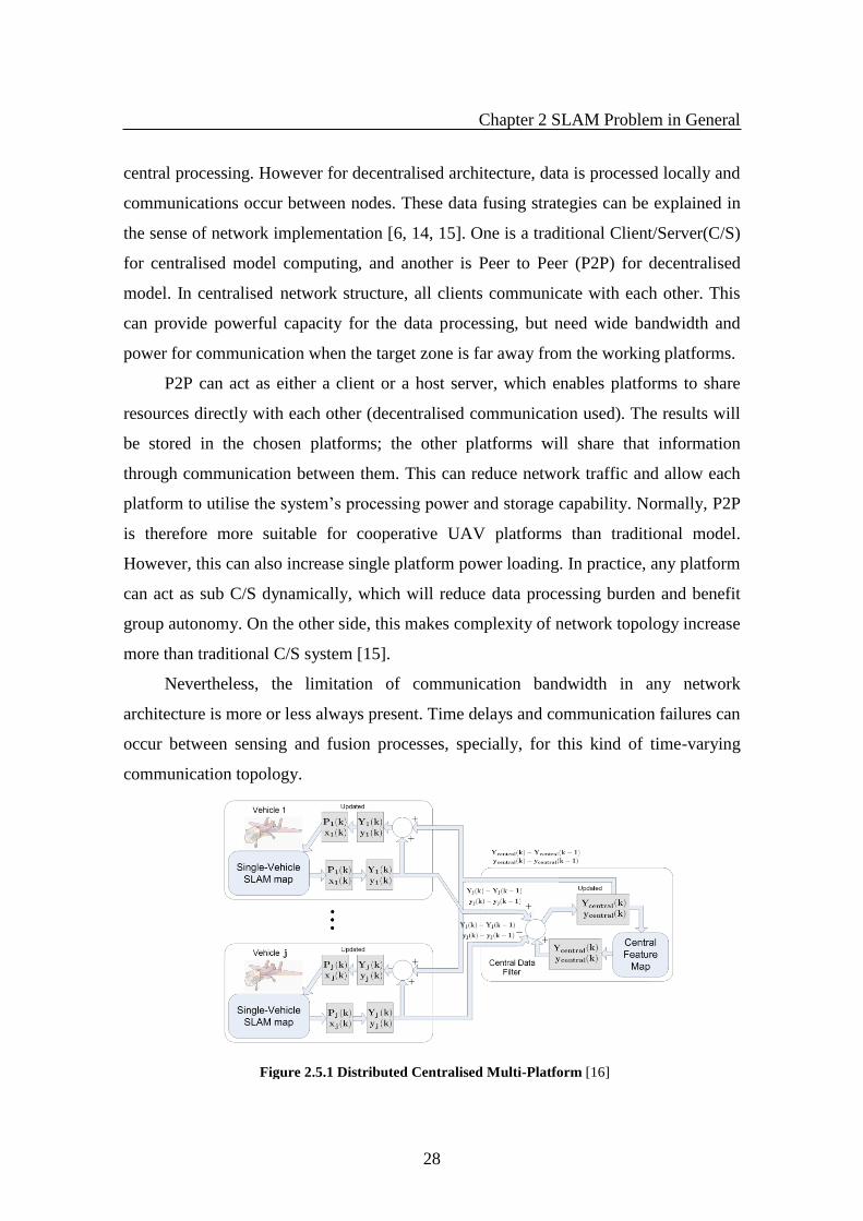
Chapter 2 SLAM Problem in General
28
central processing. However for decentralised architecture, data is processed locally and
communications occur between nodes. These data fusing strategies can be explained in
the sense of network implementation [6, 14, 15]. One is a traditional Client/Server(C/S)
for centralised model computing, and another is Peer to Peer (P2P) for decentralised
model. In centralised network structure, all clients communicate with each other. This
can provide powerful capacity for the data processing, but need wide bandwidth and
power for communication when the target zone is far away from the working platforms.
P2P can act as either a client or a host server, which enables platforms to share
resources directly with each other (decentralised communication used). The results will
be stored in the chosen platforms; the other platforms will share that information
through communication between them. This can reduce network traffic and allow each
platform to utilise the system’s processing power and storage capability. Normally, P2P
is therefore more suitable for cooperative UAV platforms than traditional model.
However, this can also increase single platform power loading. In practice, any platform
can act as sub C/S dynamically, which will reduce data processing burden and benefit
group autonomy. On the other side, this makes complexity of network topology increase
more than traditional C/S system [15].
Nevertheless, the limitation of communication bandwidth in any network
architecture is more or less always present. Time delays and communication failures can
occur between sensing and fusion processes, specially, for this kind of time-varying
communication topology.
Figure 2.5.1 Distributed Centralised Multi-Platform [16]

Chapter 2 SLAM Problem in General
29
In centralised data fusion framework, normally there is a public server acting as a
data center embedded with data processing algorithm providing a centralised platform
for data exchanging among UAVs. On the other hand in decentralised framework data
fusion is carried out based on non-control center and the platform member is able to
reorganise it when any single platform fails. The algorithm inhabited can be equally
distributed inside the group.
Normally, centralised architectures provides better precision of the UAVs
positions and constructed map while the decentralised model is more suitable for real
time and embedded system applications [62]. A decentralised structure is adopted in this
research.
There are some ideas and solutions to reduce communication cost for real time
applications. For example, we can make sub groups of platforms when chosen platforms
can communicate outside of the group. Meanwhile, we reduce information sharing to
only individual estimates of pose and covariance with part of the measurements. In
addition, we can use point to point communication instead of broadcast, and
compression by means of quantisation of sensor observations. Overall, it is open to
incorporating different methods or strategies to overcome this bottle-neck.
With network communication constraints enforced, the challenge from data fusion
for cooperative SLAM operating on the distributed platforms is much greater than that
of single SLAM. This is needed to fulfill its purpose of building a map of terrain
landmarks whilst simultaneously using these to determine self-location of the platforms.
Figure 2.5.2 Distributed Decentralised Multi-Platform [16]

Chapter 2 SLAM Problem in General
30
Apart from how to allocate and balance the loading of computation and data
communication, which largely depends on the network structure and individual platform
performance, the challenge will be mainly in fusion algorithm and methodology utilised
with distributed multi sensors.
2.6 Summary and Conclusion
The introduction of the SLAM state of the art gives an overview of SLAM,
background of this research, technical challenges with SLAM/vSLAM. A special
emphasis is given to cooperative visual SLAM, which is the focus of this research. It
acknowledges that the cooperative visual airborne SLAM is an open and challenging
area that needs to be investigated and explored for its application in real world scenario.
Therefore there is still a huge need for further research efforts in this area.
Chapter 3 Camera Imaging, Modelling and Vision Processing
31
CHAPTER 3
Camera Imaging, Modelling and Vision Processing
In this chapter, we present the theoretical and conceptual image processing
foundations. We carried out investigation on feature extraction methods suitable for
aerial imaging in terms of number of extracted features, matching rates, running time
and feature invariance. This was done for both visual and infrared bands in different
environments. Various feature extraction methods, especially variants of SIFT
algorithms were studied in-depth with comparative analysis.
3.1 Introduction
Ultimately, mapping in camera vision based SLAM is the process of inferring
three-dimensional information from 2D images captured from different viewpoints.
Therefore, understanding the camera model and vision processing is absolutely
necessary in the implementation of visual SLAM. Through camera modelling [3, 60, 61,
69] and other specific vision tools [12, 17, 22], vision information is then used to
compute properties of the 3-D world from stereo digital images. Thus this is a
fundamental aspect of this research.
As the data measured in images are just coordinates in pixels, to obtain the
relationship between 3D space and 2D images, the basic approach is to use camera
calibration (Tsai, 1986; Faugeras and Toscani, 1986)[151, 152], to establish a model (3
x 4 projection matrix) which relates pixel coordinates to 3D coordinates.
There are 12 entries with 11 camera parameters in this projection matrix. Its
parameters describe the internal geometry of the camera as well as its position and
orientation in space with regards to a fixed chosen reference frame. Therefore the
directions in 3D space from pixel measurements can be obtained through the knowledge
of the internal geometry of the camera. Furthermore, the rigid displacement - the
relative Euclidean positioning of cameras, corresponding pose in metric quantities
described in the work frame can be deduced from those calibration parameters.

Chapter 3 Camera Imaging, Modelling and Vision Processing
32
This calibration methodology is universal although it is not always practical to
have off-line camera calibration during UAV flight in the air where the deformation of
rigid body infrastructure could occur.
Furthermore, in the case of a stereo rig, there is the drawback of independent
calibration on each camera, which makes the estimated parameters redundant with a
workload of up to 11 + 11. To have further rigid displacement between the cameras
would still require a minimum estimation of 15 parameters.
Thus, an approach [146] with a non-metric nature using projective information
has emerged. This makes it suitable for utilisation with cameras of unknown internal
parameters. Only a small number of parameters need to be estimated with just geometric
information required from the different viewpoints. Applying this approach, one can
have even better understanding of the fundamental elements in the geometry of two
cameras, and naturally leading to the image formation process. It can describe the stereo
cameras' geometric relations in projective space rather than in Euclidean terms, where
only 7 parameters are used. Information is encapsulated in a fundamental matrix, which
can be obtained through stereo camera calibration.
The following section presents a brief description of the concepts and techniques
described above which are embedded in this research.
3.2 Camera Imaging and Modelling
It is a complex process to have image formation and acquisition with modern
digital technology. In the context of this research, a brief introduction is given for
camera imaging, the tailored and suited camera model, and the epipolar or two-view
geometry. This section continues with the description of the perspective camera model
corresponding to a pinhole camera. An explanation of camera parameters and their
calibration issues is presented. It is assumed throughout this section that effects such as
negligible radial distortion are ignored.
3.2.1 Camera Image Formation
In a digital camera, image formation mechanism is quite similar to that of human
vision, i.e., images are formed by light rays that are coming through the pupil, going
through the lens which then focus the light on the photo sensors of the retina for a sharp

Chapter 3 Camera Imaging, Modelling and Vision Processing
33
image. Within a camera, a CCD (charge-coupled device) or a CMOS (complementary
metal oxide) is used as photosensitive sensor, which works as Optical-Electric
Transducer, receiving light ray, and converting it as digit intensity matrix. It is
represented by monochromatic or chromatic data (RGB or CYMG filter array). Those
incident rays are the mixture of reflections (majority) from various objects within a
scene and light source.
The apparent brightness of different objects is generally assumed to be the same
regardless of the observer's angle of view under constant illumination. Such behavior is
described by lambertian reflectance model (Johann Heinrich Lambert, 1760)[147-149]
which defines an ideal diffusely reflecting surface. More technically, the
surface's luminance is isotropic, i.e., each visible point of an object appears equally
bright from all viewing, and the luminous intensity obeys Lambert's cosine law [148,
149]. The introduction of the concept for this perfect diffusion provides both theory and
well approximated mathematical model which has seen wide application in camera
imaging and computer graphics.
3.2.2 Pinhole Camera Model - Perspective Model
In order to have any point on the scene for image focusing, theoretically, a
complicated optical system is required to gather all rays from such point and accumulate
them into a single imaging point. In reality, a simpler model of focusing is introduced
by reducing the camera aperture to a point in order to have only one ray from a given
point entering the camera and hitting the image plane. In this way, a one-to-one
correspondence can be established through projection between a scene point and an
image point. In computer vision, this camera model is usually named as a perspective or
a pin-hole camera model [61], where the existing collineation maps the projective space
to the camera’s retinal plane (image reference frame): 2PP 3 . Then, in a Euclidean
world coordinate system, the coordinates of a 3D point TZYXM ],,[ and the retinal
image coordinates Tvum ],[ have the following relation: MPms~~ where s is a scale
factor, Tvum ]1,,[ and TZYXM ]1,,,[ are the homogeneous coordinates for vector m
and M respectively. P is a 3x4 matrix which can represent the collineation: 2PP 3 .
Namely, P is defined as the perspective projection matrix.
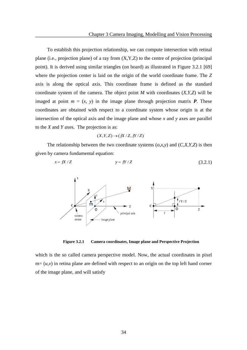
Chapter 3 Camera Imaging, Modelling and Vision Processing
34
To establish this projection relationship, we can compute intersection with retinal
plane (i.e., projection plane) of a ray from (X,Y,Z) to the centre of projection (principal
point). It is derived using similar triangles (on board) as illustrated in Figure 3.2.1 [69]
where the projection center is laid on the origin of the world coordinate frame. The Z
axis is along the optical axis. This coordinate frame is defined as the standard
coordinate system of the camera. The object point M with coordinates (X,Y,Z) will be
imaged at point m = (x, y) in the image plane through projection matrix P. These
coordinates are obtained with respect to a coordinate system whose origin is at the
intersection of the optical axis and the image plane and whose x and y axes are parallel
to the X and Y axes. The projection is as:
)/,/(),,( ZfYZfXZYX
The relationship between the two coordinate systems (o,x,y) and (C,X,Y,Z) is then
given by camera fundamental equation:
ZfXx / ZfYy / (3.2.1)
which is the so called camera perspective model. Now, the actual coordinates in pixel
m= (u,v) in retina plane are defined with respect to an origin on the top left hand corner
of the image plane, and will satisfy
Figure 3.2.1 Camera coordinates, Image plane and Perspective Projection

Chapter 3 Camera Imaging, Modelling and Vision Processing
35
replacing with (3.2.1), we can have
where pixel size xs and
ys are in width and height respectively; optical centre O is with
image coordinates (ou, ov) in pixels. Their coordinate’s relation is shown in Figure 3.2.1.
The natural deduction above is based on geometry principle; we can then simply apply
homogeneous coordinates as homogenous image coordinate )1,,(),( vuvu and
homogenous 3D real scene coordinate )1,,,(),,( ZYXZYX . More generally, the
converting between homogeneous coordinates and Euclidean ones can be depicted in
the relation written as )/,/( wvwu
w
v
u
and
)/,/,/( wZwYwX
w
Z
Y
X
, where the scale (or
space) w is applied for the universal ratio from homogenous space to Euclidean space.
Thus, the geometric projection is easily obtained using homogeneous coordinates
)3.2.3( , which can be rewritten as:
MPmZ
Y
X
o
o
w
wv
wu
vv
uu~~
10100
00
00
)4.2.3(
This is known as perspective projection with perspective projection matrix
u
x
os
xu
v
y
os
yv
u
x
Zos
fXZu
v
y
Zos
fYZv
)2.2.3( b
)3.2.3( b
)2.2.3( a
)3.2.3( a

Chapter 3 Camera Imaging, Modelling and Vision Processing
36
0100
00
00
vv
uu
o
o
P
, w is scaling factor with value Z, where the symbol m~ represents the
homogeneous vector of image pixel coordinates, and M~
is the homogeneous vector of
world coordinates. Thus, a camera can be considered as a system that performs a linear
projective transformation from the projective space 3P into the projective plane 2P .
There are only four separable projection parameters in )4.2.3( that needs to be solved, as
an arbitrary scale factor is involved in f and in the pixel size. Thus we can only solve for
the ratios x
u sf
and y
v sf
. The independent parameters vuvu oo ,,, are named
intrinsic parameters independent on the position and orientation of the camera in space.
The optical axis passes through the center of projection (camera) C, which is
orthogonal to the retinal plane. The known focal length f of the camera is the distance
between the center of projection and the retinal plane.
With the availability of the perspective projection matrix P, it is possible to recover the
coordinates of the optical center or camera.
3.2.3 General Camera Matrix and Calibration
In computer vision, a camera matrix or perspective projection matrix is a 3x4
matrix as indicated above contains the intrinsic parameters. It describes the mapping of
a pinhole camera from 3D points in the world to 2D points in an image [69, 89, 90], i.e.,
the transformation between the world frame and retinal plane (image plane).
Generally, the world coordinates in 3D a point will not be specified in a frame
whose origin is at the centre of projection and whose Z axis lies along the optical axis. If
other frames to be specified, we then have to include a change of coordinates from other
frames to the standard coordinate system by coordinates matrix transformations. Thus
we have
MPKm~~ (3.2.5)
where K is a 4x4 homogeneous transformation matrix:
103
T
T tRtRK
(3.2.6)
Chapter 3 Camera Imaging, Modelling and Vision Processing
37
The top 3x3 corner is a rotation matrix R (details in next section) that encodes the
camera orientation with respect to a given reference or world frame while the final
column is a homogeneous vector t which captures the displacement of camera from the
reference frame origin. There are 6 DoF in matrix K, of which, three for the orientation,
and other three for the translation of the camera. These parameters are known as the
extrinsic camera parameters. The 3x4 camera matrix P and the 4x4 homogeneous
transform K combine together to produce a general single 3x4 matrix C with rank three
called the camera calibration matrix ][ tRPPKC as a function of the intrinsic and
extrinsic parameters in [77]:
z
zvyv
zuxu
vv
uu
t
tot
tot
r
ror
ror
C
3
32
31
(3.2.7)
where the vectors 321 ,, rrr are the row vectors of the matrix R, and t = (tx, ty, tz). The
camera calibration matrix can then be used to transform points from the retinal plane to
points on the image plane in arbitrary space and vice versa.
The nature of camera calibration is to relate the locations of pixels in the image
array to scene points. Each pixel is imaged by perspective projection, which
corresponds to a ray of points in the scene. Camera calibration is the first step towards
computational computer vision.
The camera calibration problem is then mathematically required to determine the
equation for this ray in absolute world coordinate system of the scene. This includes the
solution of both the exterior and interior orientation parameters which are the position
and orientation of the camera and the camera constant. In order to obtain the relation of
image plane coordinates and absolute coordinates, the location of the principal point, the
aspect ratio and lens distortions must be determined. The camera calibration problem
normally involves determining two sets of parameters: the extrinsic parameters for rigid
body transformation (exterior orientation) and the intrinsic parameters for the camera
itself (interior orientation).
Generally, in camera calibration, the exterior orientation problem should be
solved before attempting to solve the interior orientation problem, since we must know

Chapter 3 Camera Imaging, Modelling and Vision Processing
38
how the camera is positioned and oriented in order to know where the calibration points
project into the image plane. Once we know where the projected points should be, we
can use the projected locations and the measured locations in image, to determine the
lens distortions and correct the location of the principal point and the image aspect ratio.
The solution to the exterior orientation problem must be based on constraints that are
invariant to the lens distortions and camera constant, which will not be known at the
time that the problem is solved.
The estimation of the camera calibration matrix has detailed description in [69, 89,
90].
3.3 Epipolar Geometry
3.3.1 Introducing Epipolar Geometry
In this section, we use references [23, 70, 78].
The epipolar geometry is the projective geometry of two views, which exists
between two-camera systems (stereo vision). As depicted in Figure 3.3.1, it is formed
by the intersection of the image planes. The shape of the plane is like a pencil, which
has a baseline as an axis. The baseline is the collinear link of the two camera centres.
This geometry is independent of scene structure, and only relies on the cameras' internal
parameters and relative pose.
Having the pinhole camera model in epipolar geometry, there are a number of
geometric relations between the 3D points and their projections onto the 2D images that
lead to constraints between the image points. With references to Figure 3.3.1, the two
cameras are represented by C1 and C2. Point m1 in the first image and m2 in the second
image are the imaged points of the 3D point M. Points e1 and e2 are the so-called
epipoles, which are the intersections of the line joining the two cameras C1 and C2 with
both image planes or the projection of the cameras in the opposite image.

Chapter 3 Camera Imaging, Modelling and Vision Processing
39
An epipolar pencil plane is formed by triangulated points C1, M and C2. The lines
lm1 and lm2 are named epipolar lines which are formed when the epipoles (e1,e2) and
image points (m1,m2) are linked respectively, i.e., the intersection of epipolar plane and
two image planes. Different world points can have different epipolar lines which all go
through the same two epipoles forming the so called pencils of epipolar lines as
depicted in Figure 3.3.2.
The image point m2 of M is restricted to lie on the epipolar line lm1 of point m1.
Same to the image point m1 of M on I1, it is restricted to lie on the epipolar line lm2 of
point m2. This corresponds to the epipolar constraint which is usually the motivation of
epipolar geometry to search for corresponding points in stereo matching. To visualise it
in difference, the epipolar line lm1 is the intersection of the epipolar plane with the
second image plane I2. This means that image point m1 can correspond to any 3D point
(even at infinity) on the line C1M and that the projection of C1M in the second image I2
is the line lm1. The same principle is applied to image point m2 as well. All epipolar lines
of the points in the first image pass through the epipole e2. The pencil of planes
containing the baseline C1C2 is formed thereafter.
Figure 3.3.1 Epipolar Geometry
Figure 3.3.2 Pencils of Epipolar Lines

Chapter 3 Camera Imaging, Modelling and Vision Processing
40
The above definitions are symmetric in a way that the point m1 must lie on the
epipolar line lm2 of point m2. To have algebraical expression of epipolar constraint when
matching m1 and m2, the following equation in image coordinates (pixels) needs to be
satisfied with colinearity:
0~~12 mFmT (3.3.1)
where F is the 3 × 3 fundamental matrix. With fundamental matrix in its transpose
form [69], combining equation (3.2.5) in the case of first camera coincides with the
world coordinate system, we can then have
MICms x
~0~
333111 (3.3.2)
MtRCms~~
222 (3.3.3)
here C1 and C2 are used to represent the camera calibration matrices (with intrinsic
parameters only) for each camera as in previous section. R and t describe a
transformation (rotation and translation) from the first coordinate system to the second
one. The fundamental matrix can then be written in the form:
1
12
RCtCF x
T (3.3.4)
where xt is the antisymmetric matrix representation of the cross product translation
vector [t] in projective space [69].
The fundamental matrix satisfies the condition of any pair of points corresponding
as21 mm in the two images. Defined up to a scalar factor, the fundamental matrix F is
of rank 2 with 7 DoF(7 independent parameters among the 9 elements), where R is a
3x3 rotation matrix and [t]is a 3D translation vector.
In the fundamental matrix, if the intrinsic parameters of the camera are known in
equation (3.3.4), then from the fundamental matrix, the essential matrix [69] can be
decomposed as:
RtE x (3.3.5)
E is the essential matrix if and only if two singular values are equal (and third=0)
T0)VUdiag(1,1,

Chapter 3 Camera Imaging, Modelling and Vision Processing
41
which has 5 DoF (3 for R, 2 for t up to scale).
Both E and F enable full reconstruction of the epipolar geometry. E only encodes
information on the extrinsic parameter which gives the pose relationship of the two
cameras. F encodes information on both intrinsic and extrinsic parameter. We can also
have the compact relationship expressed in intrinsic, essential and fundamental matrices
as:
1
12
ECCF T (3.3.6)
12 FCCE T (3.3.7)
The details to estimate fundamental martix and essential matrix can be found in the
literature [69, 70, 78].
Fundamental matrix [61, 63] is used to describe the projective structure of stereo
images. Camera extrinsic parameters define the relation between image plane and world
frame, which can be expressed by essential matrix [61] that is the natural link between
the epipolar constraint and extrinsic parameter of the stereo system.
If a set of point correspondences from two views can determine the fundamental
matrix uniquely, then the scene and cameras position can be reconstructed from these
correspondences alone. Any of those two reconstructions based on these
correspondences has projective equivalence. Therefore, robust methods for determining
the correspondences from two images are especially important in order to have accurate
camera calibration. These correspondences in image data are usually in the form of
corners (high curvature points), as they can be easily represented and manipulated in
projective geometry. There are various corner detection algorithms. In our research,
instead of using epipolar constraint, we employ SIFT [12, 21] and SURF [17] algorithm
for feature extraction and matching in order to have correct correspondences from two
images.
Finding corresponding corners from two images is a key step and form a
fundamental part of epipolar analysis. Features are estimated in two images
independently, and the matching algorithm needs to pair up the same feature or corner
points correctly. Thereafter, we can build up corresponding triangulation in depth
estimation. The accuracy of feature matching will largely determine the end results of
depth estimation, which is crucial to 3D reconstruction.
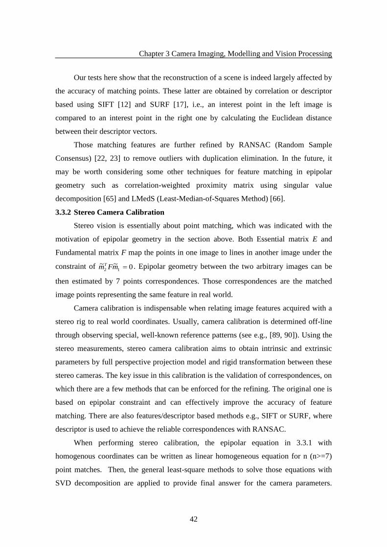
Chapter 3 Camera Imaging, Modelling and Vision Processing
42
Our tests here show that the reconstruction of a scene is indeed largely affected by
the accuracy of matching points. These latter are obtained by correlation or descriptor
based using SIFT [12] and SURF [17], i.e., an interest point in the left image is
compared to an interest point in the right one by calculating the Euclidean distance
between their descriptor vectors.
Those matching features are further refined by RANSAC (Random Sample
Consensus) [22, 23] to remove outliers with duplication elimination. In the future, it
may be worth considering some other techniques for feature matching in epipolar
geometry such as correlation-weighted proximity matrix using singular value
decomposition [65] and LMedS (Least-Median-of-Squares Method) [66].
3.3.2 Stereo Camera Calibration
Stereo vision is essentially about point matching, which was indicated with the
motivation of epipolar geometry in the section above. Both Essential matrix E and
Fundamental matrix F map the points in one image to lines in another image under the
constraint of 0~~12 mFmT . Epipolar geometry between the two arbitrary images can be
then estimated by 7 points correspondences. Those correspondences are the matched
image points representing the same feature in real world.
Camera calibration is indispensable when relating image features acquired with a
stereo rig to real world coordinates. Usually, camera calibration is determined off-line
through observing special, well-known reference patterns (see e.g., [89, 90]). Using the
stereo measurements, stereo camera calibration aims to obtain intrinsic and extrinsic
parameters by full perspective projection model and rigid transformation between these
stereo cameras. The key issue in this calibration is the validation of correspondences, on
which there are a few methods that can be enforced for the refining. The original one is
based on epipolar constraint and can effectively improve the accuracy of feature
matching. There are also features/descriptor based methods e.g., SIFT or SURF, where
descriptor is used to achieve the reliable correspondences with RANSAC.
When performing stereo calibration, the epipolar equation in 3.3.1 with
homogenous coordinates can be written as linear homogeneous equation for n (n>=7)
point matches. Then, the general least-square methods to solve those equations with
SVD decomposition are applied to provide final answer for the camera parameters.

Chapter 3 Camera Imaging, Modelling and Vision Processing
43
There are many methods, such as linear, nonlinear and robust methods in literature [69,
89, 90], which can be applied to get this solution.
Apart from the above, we can also integrate the single camera calibration methods
with stereo measurements for the calibration of stereo camera task.
Following this approach, each camera starts with its own calibration to determine
the camera constants, location of the principal point, correction table for lens distortions,
and other intrinsic parameters. Once finished, it is possible to solve the relative
orientation problem and determine the baseline by other means, such as using the stereo
cameras to measure points that are a known distance apart. This fully calibrates the rigid
body transformation between the two cameras. Point measurements can then be
gathered in the local coordinate system of the stereo cameras. Since the baseline has
been calibrated, the point measurements will be in real units and the stereo system can
be used to measure the relationships between points on objects in the scene. It is not
necessary to solve the absolute orientation problem, unless the point measurements
must be transformed into another coordinate system.
It is important to note that camera calibration methods for both single and stereo
in many ways have similar technical and theoretical background using the 3D
calibration target, i.e., conducting camera calibration is via observing a calibration
target which consists of two or three planes orthogonal to each other, whose 3D
geometry dimension is known with good precision. However, this approach requires
expensive equipment and elaborate installation.
When it comes to extrinsic parameters, stereo cameras have the relationship
between two cameras which should be reflected in extrinsic parameters.
In recent years, there has been seen increasing interest in camera self-calibration
methods. Self-calibration for stereo cameras refers to the automatic determination of
extrinsic and intrinsic camera parameters of a stereo rig from almost arbitrary image
sequences. Therefore, such methods allow the camera parameters to be recovered while
the sensor is still in use without presenting of any special calibration object. This is
considered more effective and practical, and is available and handy to use. Most of
available tools can meet both stereo and single camera calibration requirements. One of
them is the Matlab calibration toolbox given in [150].

Chapter 3 Camera Imaging, Modelling and Vision Processing
44
3.4 Camera Imaging based Vision Processing
Image features extraction and matching is the prerequisite and fundamental aspect
of vSLAM application. The success of vSLAM largely relies on the accuracy of features
extracted from the corresponding images taken from the geographical environment by
electronic optical cameras.
A feature could be classified as a corner, edge, or a pixel region with a large
histogram of different colours [12]. To identify the corresponding points in two
different images is the premise for further processing. In vSLAM, they are used to solve
for 3D structure from multiple images, stereo correspondence, and motion tracking,
where a feature is used to reference the vehicle's position to a known location.
In this thesis, the most popular feature tracking algorithm SIFT and its variants
[12, 17] are to be investigated on both visual and infrared images in vision based
airborne navigation problems.
Nowadays, high performance imaging sensors have become the common facilities
on unmanned vehicles, including both visible spectrum and infrared cameras.
In order to make utmost of the informative imaging, it is necessary to have the
good understanding of feature characteristics, which is presented by certain image
processing techniques (SIFT and its variants in this research). The contrast of thermal
infrared imaging is generally lower compared to that of traditional visible images. This
gives rise to a new challenge when infrared images (i.e. thermal infrared in this
research) are to be used in autonomous vision based navigation tasks. Therefore, the
study conducted on images of both visible and infrared bands can give insight views of
their natures. It is the premise of the later application in the mapping for the navigation.
This chapter presents a comprehensive analysis on the most popular robust
feature detection/description methods - Scale Invariant Feature Transform (SIFT) and
careful selections of its various implementation including Speeded-Up Robust Features
(SURF)[17], ASIFT[102], VL_SIFT, VL_DSIFT, VL_PHOW (GRG, HSV,
OPPONENT) [93].
Lowe presented standard SIFT in [12], which was successfully used in image
mosaic, recognition, and lately visual based navigation [40]. On the other hand, SURF
and other various SIFT provided alternatives to either speed up, or provide more
Chapter 3 Camera Imaging, Modelling and Vision Processing
45
accurate descriptors as claimed originally for automatic feature extraction and matching.
The use of such alternatives has been taken into considerations in terms of their
application in various environments within the literature [94-98]. Those experimental
analyses are valuable to other users for specific application. However, there are limited
research works in the literature that studied the automatic feature processing in infrared
images for target recognition and tracking applications in vision based navigation
applications [104, 105] from aerial platforms [106, 107]. No in depth investigations
linked to feature processing in different modalities of infrared and visible imaging
bands have been conducted.
Understanding the performance of the main robust feature detectors/descriptors
such as SIFT over these imaging modalities becomes inevitable in our research.
Affine-SIFT is a successful modification of the standard SIFT, as it is an affine
transformation based algorithm. We believe it can be more suitable for aerial images
snapped onboard. VL_FEAT is a feasible and creditable library tool that provides
several SIFT implementations including colour descriptor of SIFT. This can be
conceptually a potential competitor to the original SIFT. The investigation is therefore
carried out with a batch of SIFT variants in aerial imaging environment aiming to seek
the best candidate for our application.
In particular, the analysis will focus on the performance of feature extraction and
matching algorithms.
3.4.1 SIFT- Scale Invariant Features Transform
According to David G. Lowe [12], the properties of image features make them
suitable for matching differing images of an object or scene. Those features are
generally invariant to image scaling and rotation, and partially invariant to changes in
illumination and camera viewpoint. Those features are well localised in both the spatial
and frequency domains. This reduces the probability of disruption by occlusion, clutter
or noise.
The SIFT algorithm was published by David Lowe [12] who was inspired by
response properties of complex neurons in visual cortex, to detect distinctive keypoints
from images with a corresponding computed descriptor.
Chapter 3 Camera Imaging, Modelling and Vision Processing
46
Firstly, it uses scale-space extrema to efficiently detect the location of those stable
keypoints located at maxima and minima of a difference of Gaussians (DoG) function
applied in scale space. The latter means that an image pyramid is built using resampling
between each level. Then, a very distinctive descriptor is created based on an orientation
histogram at cells (each is a 4x4 squared grid subregion around the interest point),
which results in a 128 dimensional vector. This vector is formed by the gradient in
different directions (the gradient orientation is quantised to 8 angles in each cell, and the
sum of gradient magnitude is conducted and binned along each direction) and the
keypoint orientations are represented by dominant orientations. Thus, each keypoint is
represented by the scale, orientation, location and the gradient descriptor, so that it can
achieve invariance to image translation, scaling and rotation. Therefore, such distinct
descriptors make it possible to find a match under variations in illumination, 3D
projection and even six degree of freedom affine transform. This makes SIFT a very
competitive candidate for an automatic feature detection task. The following outlines
the major stages of computation that generate the set of SIFT features [12]:
Scale-space extrema detection: The first stage of computation searches over all
scales and image locations, which is implemented efficiently using a DoG function,
to identify potential interest points that are invariant to both scale and orientation.
Keypoint localisation: At each candidate location, a detailed model is fit to
determine location and scale. Keypoints are selected based on measures of their
stability.
Orientation assignment: One or more orientations are assigned to each keypoint
location based on local image gradient directions. All future operations are
performed on image data that have been transformed relative to the assigned
orientation, scale, and location for each feature. Therefore, it can provide invariance
to these transformations.
Keypoint descriptor: Local image gradients are measured at the selected scale in the
region around each keypoint. These are transformed into a representation that
accommodates for significant levels of local shape distortion and change in
illumination.

Chapter 3 Camera Imaging, Modelling and Vision Processing
47
The name of SIFT comes from the fact that it transforms image data into scale-
invariant coordinates relative to local features. It can generate large numbers of features
that densely cover the image over the full range of scales and locations, which is very
important for feature extraction.
The quantity of features is particularly important for object recognition, where the
ability to detect small objects in cluttered backgrounds requires that at least three
features be correctly matched from each object for reliable identification [12].
3.4.2 Affine- SIFT
Since Lowe's initial work on SIFT, there have been several variants of SIFT
developed through either modification of keypoints or descriptor formulation. Those
variants of SIFT show various responses in the presence of different environments [94-
98]. Some of them are either a bit obsolete or have been already examined under various
combinations in the literature [94-98]. In our application, aerial images acquired from
UAV are far from the normal condition, where strong affinity transformation and 3D
illumination changes are involved. This motivated us to carefully test several of SIFT
variants such as Affine-SIFT.
As a member of SIFT family, Affine-SIFT (ASIFT) was proposed by J. M. Morel
[102]. In ASIFT, affine transformation parameters are adopted to correct images with
the intension of resolving strong affine issues. The latter is one of the weaknesses of
standard SIFT. ASIFT takes the common sense of local deformations in a single view
can be approximated by several different local affine transforms by simulating the
rotation of camera's optical axis. An image affine transformation model in the concise
form of fdvcuebvauIvuI ,),( is used to simulate the variation of
viewpoint from remote distance. The parameters of fdceba ,,,,, are determined by
a series of translation, scaling, rotation, shearing, squeezing of image affine deformation.
In ASIFT, all those parameters are actually approximated by rotation in first place
followed by tilt )(t transformation as ),(, vtuIvuI . They are practically achieved
by means of changing the longitude angle ø and the latitude angle θ within a certain
range.

Chapter 3 Camera Imaging, Modelling and Vision Processing
48
The longitude angle ø is formed by the normal plane of the measured object and
the mapping plane of the camera optical axis due to the movement of camera causing
the deformation of the object imaging. The camera optical axis then makes a latitude
angle θ with the normal to the image plane I. Both parameters are classical coordinates
on the observation hemisphere. By applying a dense set of rotation and simulated tilts,
the affine transformation of images can be obtained, where keypoints detection and
description are to be carried out.
3.4.3 Variants SIFT in VLFeat
The VLFeat is an open source library [93] implementing various algorithms of
SIFT, including VL_SIFT, fast SIFT- VL_DSIFT, and VL_PHOW with visual
descriptors of RGB (Red, Green, Blue), HSV (Hue, Saturation, Value) and Opponent
based respectively.
3.4.3.1 VL_SIFT
VL_SIFT is an alternative version of standard SIFT, where SIFT frames are
expressed in the standard image reference with the y axis pointing downward and x axis
facing right forward. The frame orientation θ and descriptor are calculated in the same
reference, a bin for each descriptor element is indexed by yx,, , and the histogram is
vectorised in a way so that the fastest varying index is for orientation θ and the slowest
one is y.
3.4.3.2 VL_DSIFT
According to [93], VL_DSIFT is the fast version of SIFT based on dense SIFT. It
is equivalent to running SIFT on a dense gird of locations (a regular grid with a spacing
of M pixels, where M rely on the size of the image and richness of features) at a fixed
scale and orientation. There are a few issues in VL_DSIFT.
Bin size vs keypoint scale. The descriptor size in DSIFT is specified by a single
parameter, size, which is a controller for the size of a SIFT spatial bin in pixels.
However in Lowe's standard SIFT descriptor, a multiplier (magnify) links the bin
size to the SIFT keypoint scale, is defaults to 3. Therefore, bin size of 5 in a DSIFT
descriptor matches a scale 5/3=1.66 of standard SIFT keypoint.

Chapter 3 Camera Imaging, Modelling and Vision Processing
49
Smoothing. The standard SIFT descriptor uses Gaussian scale (s) to smooth the
image, which is in default in DSIFT, equivalent to a convolution by a Gaussian of
variance 25.02 s . The nominal numerical adjustment 0.25 is accounted for the
smoothing induced by the camera CCD.
3.4.3.3 VL_PHOW (Pyramid Histogram of visual Words)
PHOW features [28, 29] are actually a variant of dense SIFT descriptors extracted
at multiple scales. Its visual version combines colour information in generating
descriptors of image directly based on colour channels of the images through the
decompositions in HSV or RGB or Opponent channels and stacks them up. Histogram
calculation in standard SIFT is on gray image combining intensity in 1D from three
RGB channels. It is not invariant to colour changes. Taking advantage of intensity of 3
channels is therefore able to have better description on key points. For feasible and
efficient computing, VL_PHOW is the wrapper of PHOW features. These colour
descriptors have their specific distinct nature with increasing wide-spread use in certain
area such as object classification.
Colour information could contribute to the improvement of the identification for
binocular disparities in order to recover the original three-dimensional scene from two-
dimensional images. Colour makes the matches less sensitive to occlusion knowing that
occlusion most often causes colour discontinuities.
There is no local spatial information in colour histograms which are inherently
pixel-based. It is different from derivative-based standard SIFT descriptors which
makes use of local spatial information. Each of these three types of colour descriptor
has 3x128 dimensions per descriptor, 128 per channel, with histogram calculated
separately in each channel of corresponding colour space with no invariance properties
in descriptors.
The large descriptor may probably have side effects such as being time consuming
on matching computation. The basic principles related to this technique are given here:
HSV-SIFT, HSV (Hue, Saturation, Value) as a colour model, describes colours
(hue or tint) in terms of their shade (saturation or amount of gray) and their
brightness (value or luminance). HSV is one of the two (another is HSL stands for

Chapter 3 Camera Imaging, Modelling and Vision Processing
50
hue, saturation, and lightness) most common cylindrical-coordinate representations
of points in an RGB colour model. These two representations transform the
geometry of device-dependent RGB models to be more intuitive and perceptually
relevant than the Cartesian (cube) representation. The HSV descriptor [29]
computes SIFT descriptors over all three channels.
RGB-SIFT, RGB stands for the colours of Red, Green and Blue, which is the
most common additive primaries on-screen colour mode. Colours on a screen are
displayed by mixing varying amounts of red, green and blue light. Each unique
RGB device has unique HSL and HSV spaces to accompany it. Numerical HSL or
HSV values describe a different colour for each base RGB space [27]. For the RGB-
SIFT descriptor, SIFT descriptors are computed for every RGB channel
independently.
Opponent-SIFT, Opponent colour model is the better model of HVS (Human visual
system) due to the fact that perception of colour is usually not best represented in
RGB.
Opponent colour space has three components [97]: luminance component
2/1 GRO in red space, blue-yellow channel .6/22 BGRO
Both of them describe the colour information in the image. The channel
3/3 BGRO is equal to the intensity information, and there is no invariance
property inside.
Two opponent SIFT descriptors are computed independently on channels O1 and O2.
The SIFT descriptor computed on O3 is identical to the geometrical descriptor.
The PHOW descriptor combines these colour information to have the more
informative description of distinctive features. It is useful in scene classification
with colour information included, and differ from just dense SIFT only with
different bin sizes and smoothing to achieve scale invariance.
3.4.4 SURF- Speed up Robust Features
Partly inspired by SIFT, SURF utilises corners and blobs for their robustness to
image transformations. It was first presented by Herbert Bay et al. in 2006 with the
objective of developing both a detector and a descriptor that is faster to compute while

Chapter 3 Camera Imaging, Modelling and Vision Processing
51
not sacrificing performance [17].
Its detection process is based on the Hessian matrix. Instead of constructing the
Hessian using Gaussians and second order partial derivatives, SURF approximates this
operation with encapsulated rectangular box filters using integral images by the
convolution of the original image. Using a box filter on the integral image as a fast
approximation to the determinant of the Hessian - a very basic Laplacian-based
detector, SURF offers improved speed at the feature detection stage. When it comes to
feature description, SURF has been tuned towards high recognition rates with Haar
wavelet transform to provide a valid alternative to the SIFT descriptor. Same as SIFT,
SURF descriptor is generated through Histogram of Gradients (HoG) by capturing the
distribution of gradients within the assembling pixels. This is then constructed on the
sums of 2D Haar wavelet responses where the calculation takes place in a 4x4 subregion
around each interest point. It consists of the sum of gradients dx, dy, |dx|, |dy| for each
cell.
SURF relies on integral images to reduce the computation time and is therefore
called the 'Fast-Hessian' detector. On the other hand, it describes a distribution of Haar-
wavelet responses within the interest point neighborhood, again, using integral images
for speed.
SIFT and SURF algorithms employ slightly different ways of detecting features
[12, 17]. SIFT builds an image pyramids by filtering each layer with Gaussians of
increasing sigma values and taking the difference. On the other hand, SURF creates a
'stack' without adopting 2:1 down sampling for higher levels in the pyramid, resulting in
images of the same resolution [20, 21]. Based on integral images, the stack is filtered in
SURF by a box filter approximation of second-order Gaussian partial derivatives, as
integral images allowing computation of rectangular box filters in near constant time
[21].
Moreover, only 64 dimensions are used in SURF, reducing the time for feature
computation and matching, and increasing simultaneously the robustness. A new
indexing step is presented based on the sign of the Laplacian, which increases not only
the matching speed, but also the robustness of the descriptor.
The major stage for computing features extraction with SURF method is

Chapter 3 Camera Imaging, Modelling and Vision Processing
52
summarised as follows [17].
1. Calculate the integral image representation for fast box filtering.
2. Calculate the determinant response for the search of candidate feature points
under a Hessian based scale-space pyramid constructed by fast filtering. This
is later performed by approximating the Hessian as a combination of box
filters.
3. Perform non-maximal suppression for further filtering and reduction of the
obtained candidates in order to refine stable points with high contrast [12].
Assign each remaining point with its position and scale.
4. Calculate and assign the orientation to each interest point by finding a
characteristic direction using Haar-wavelet responses with Gaussian weights.
5. Feature descriptor is obtained based on the characteristic direction to provide
rotation invariance.
6. Normalisation is applied to the descriptor vector for luminance invariance.
3.4.5 Feature Matching and RANSAC Outlier Removal
In stereo vision based navigation tasks, the core for features detection and
description is to find correspondences between two images of the same scene or object.
This is achieved by the process of feature matching.
The search for discrete image correspondences generally includes three main
steps. First, “interest points” are selected at distinctive locations in the image, such as
corners, blobs, edges and T-junctions. The most valuable property of an interest point
detector is its repeatability, i.e., whether it reliably finds the same interest points under
different viewing conditions.
Then, a feature vector is created to represent the neighborhood of every interest
point. This descriptor has to be distinctive and, at the same time, robust to noise,
detection errors as well as geometric and photometric deformations.
Finally, the descriptor vectors are matched between different images. The
methods used in features matching are still based on a distance between the vectors e.g.,
the Mahalanobis or Euclidean distance.

Chapter 3 Camera Imaging, Modelling and Vision Processing
53
Descriptors constructed in SIFT and SURF can provide up to 128 and 64 elements
vector respectively for each salient feature. The dimension of the descriptor has a direct
impact on the time this process takes. A lower dimension (SURF) is therefore desirable
for speeding up, which is crucial for on-line applications. However, the accuracy may
not be as for SIFT whose descriptor is distinctive and relatively fast. The high
dimensionality of the descriptor is a drawback of SIFT for real time applications.
Based on those distinctive and unique descriptors, matched features can be
obtained through least Euclidean distance between descriptors according to the nearest
neighbour's principle.
The nearest neighbour is defined as the keypoint with minimum Euclidean
distance to the feature of interest. Practically, this normally uses a more effective
measure obtained by comparing the distance of the closest neighbour to that of the
second-closest neighbour [12].
Generally, the obtained and the matched features cannot be guaranteed to be
perfect due to the similarity of dense features or errors caused by inherent noise.
Therefore, to further refine the matching accuracy, RANSAC [19] is used to discard
outliers in order to find the best matches.
Random Sample Consensus (RANSAC) [22, 23] is a general framework for
model fitting in the presence of outliers. It is an iterative method of finding the best
model for a set of data by generating a hypothesis from random samples and verifying it
on the data. To apply RANSAC for the removal of outliers, the following steps are
followed:
1 A set of points (minimum four feature pairs) are randomly selected as free
parameters.
2. Generate affine model (e.g. Homography matrix H) on sample data points.
3. Test other points against this model.
4. Get inliers as points complying with the model and reject the rest as outliers.
5. Compute average error of all inliers.
6. Re-estimate model with inliers included.
7. Repeat steps 3-6 until error is tolerably small (or non-decreasing).

Chapter 3 Camera Imaging, Modelling and Vision Processing
54
In SLAM, the matched features can be refined in certain cases when the descriptor
failed to provide enough feature accuracy.
3.5 Vision Processing in SLAM
In visual SLAM, vision processing via feature extraction and matching provides
the measurement fed to the data filtering for updating the estimation. The good
integration of vision and SLAM will pave a path for the success of the mapping and
navigation.
In visual SLAM, features are first extracted from a set of reference images and
stored in a database. A new image is matched by individually comparing each feature
from the new image to this previous database and finding candidate matching features
based on Euclidean distance of their feature descriptor using nearest-neighbour
principle.
Keypoint descriptors are normally distinctive, allowing a single feature to find its
correct match with good probability in a large database of features. In addition,
RANSAC is utilised in order to further refine the matching accuracy in presence of the
outliers.
With landmarks (features in images) extraction and data association in place,
vSLAM process can be considered as a three steps scheme:
1. Predict the current state estimate using the INS data.
2. Update the estimated state from re-observing landmarks.
3. Add new landmarks to the current state.
The first step is to use data filtering for prediction with new data from INS and to
obtain the possible state for next step. It is simply the initialisation for the control of
UAV based on previous estimated state.
In the second step the re-observed landmarks are combined with the estimate of
the current position to estimate where the landmark should be. There is usually some
difference that is called the innovation [4]. The innovation is basically the difference
between the estimate value and the actual value based on what the UAV is able to see.
Usually, the uncertainty of each observed landmark is also updated to reflect recent
changes.

Chapter 3 Camera Imaging, Modelling and Vision Processing
55
In the third step, new landmarks are added to the state to augment state
matrix/vector. This is done using information about the current position and information
the relation relating new landmark and old landmarks.
The above procedure will be executed iteratively in a loop.
3.6 Investigation on SIFT Features in Visible and Infrared Images
For the purpose of visual navigation for air vehicles, the aerial image
characteristics were examined through the performance of the above feature extraction
methods. A series of experiments were carried out under different image format
captured by different sensors, i.e., visible and thermal infrared camera respectively.
Thermal infrared image normally has much lower contrast compare to the traditional
visible images. It can introduce much more blur on the visual quality of pictures. This
will probably give more challenges for features extraction and matching when applied
to vSLAM, especially in aerial scenarios.
Experiments presented in this thesis aimed to investigate both visible and infrared
aerial imaging and the overall performance of those feature extraction methods under
changes in scale, rotation, blur, illumination and affine transformation through varying
image sampling rates.
3.6.1 Experiment Requirements and Parameters Settings
Several metrics are used to evaluate the detection performance for each method,
i.e., processing time, number of matching points and matching rates.
The processing time is one of the analysis criteria of this experiment. The
evaluation time is a relative result, which only shows the tendency of those methods’
time cost. It has a tight relationship with the size of the test images and the parameters
of the algorithm, such as the distance ratio [25]. The experiments were based on an Intel
Core i5-M450 2.40GHz CPU platform. The total time is counted for the complete
processing, including feature detection and matching. A algorithm parameters are set
according to the original works [12, 17, 93, 102] with varying feature matching distance
threshold. In addition, to verify the correctness of the feature matching, RANSAC [22-
24] has been utilised in the tests to detect inliers and to reject inconsistent matches.
Results for both processing with and without RANSAC are included in the experiments

Chapter 3 Camera Imaging, Modelling and Vision Processing
56
3.6.2 Initial Tests
Both RANSAC and matching distance threshold directly affect the final number
of matched points and matching rates in vSLAM. We start with the validation of
features extraction and corresponding matches based on various distance threshold
settings using with RANSAC. These initial tests was conducted on selected standard
SIFT and OpenSURF (v1.0) with default parameters as in [12, 17]. The achieved results
will be used as a reference later when optimising parameters.
3.6.2.1 Sample Images
Images used comprise both visible and infrared as indicated in Figure 3.6.1 and
Figure 3.6.2 [26], Figure 3.6.3 and Figure 3.6.4 [27]. They were sampled in EO
(Electro-Optical) and infrared videos respectively. These images were taken from
websites [26] and [27]. Two groups of examples have been chosen as samples for our
experiments.
1802v.bmp
1810v.bmp
1802i.bmp
1810i.bmp
Figure 3.6.1EO images Figure 3.6.2 IR images
Figure 3.6.1 shows visible aerial images [26], while Figure 3.6.2 shows infrared
counterparts taken by infrared cameras. The further test is carried out with Figure 3.6.3,
and Figure 3.6.4 [27]. Table 3.6.1 shows test results.
UAVEOFrame 1.jpg
UAVEOFrame 2.jpg
UAVIRFrame 1.jpg
UAVIRFrame 2.jpg
Figure 3.6.3 EO images Figure 3.6.4 IR images
3.6.2.2 Matching with RANSAC
Figure 3.6.5 and Figure 3.6.6 present with the effects of RANSAC applied with
SIFT while Figure 3.6.7 and Figure 3.6.8 show results with SURF. The pictures clearly
show the effectiveness of RANSAC algorithm that can remove false matches during
this processing.

Chapter 3 Camera Imaging, Modelling and Vision Processing
57
Figure 3.6.5 Features matching with SIFT for EO images: LHS without
RANSAC(313matches), RHS with RANSAC(295matches)
Figure 3.6.6 Features matching with SIFT for IR images: LHS without RANSAC
(98matches), RHS with RANSAC (94matches)
Figure 3.6.7 Features matching with SURF for EO images: LHS without
RANSAC(69 matches), RHS with RANSAC(65 matches)
Figure 3.6.8 Features matching with SURF for IR images: LHS without RANSAC(46
matches), RHS with RANSAC(42 matches)
100 200 300 400 500 600 700
50
100
150
200
250
100 200 300 400 500 600 700
50
100
150
200
250
100 200 300 400 500 600 700
50
100
150
200
250
100 200 300 400 500 600 700
50
100
150
200
250
100 200 300 400 500 600
50
100
150
200
100 200 300 400 500 600
50
100
150
200
100 200 300 400 500 600
50
100
150
200
100 200 300 400 500 600
50
100
150
200

Chapter 3 Camera Imaging, Modelling and Vision Processing
58
3.6.2.3 Matching Comparison in Various Thresholds
The matching distance threshold directly affects both final number of matches and
matching rates, which are key issues in vision processing when utilised in vSLAM.
Tests here were only conducted for the inherent relation of matching – threshold. The
initial tests were implemented to evaluate matching performance of the two chosen
algorithms by varying the distance threshold with and without application of RANSAC.
Parameters of the algorithms are set to default values in [12, 17]. Table 3.6.1 gives the
results of varying matching threshold.
Table 3.6.1 Matching threshold based comparison in SIFT and SURF (without/with RANSAC) for
EO and IR images
Algorithm
Images/threshold
SIFT (without/with Ransac)
SURF (without/with Ransac)
Total time
(s) (1st/2nd
image)
Total
keypoints
(1st/2nd
image)
Matched points/rate
(to 1st/2nd image)
Total time
(s) (1st/2nd
image)
Total
keypoints
(1st/2nd
image)
Matched
points/rate
(to 1st/2nd image)
EO pictures:
Visible – Visible
1802v.bmp–
1810v.bmp
0.55
9.688 /10.00
853/728
238(.28/.33)
/234(.28/.3)
0.421/0.608
74/76
64(0.86/0.84)
/59(.8/.78)
0.75
9.578/10.448
853/728
332(.39/.46)
/291(.33/.4)
0.390/0.640
74/76
67(.9/.88)
/59(.8/.78)
0.95
10.374/10.503
853/728
619(.724/.85)
/325(.38/.45)
0.637/0.638
74/76
71(.96/.93)
/59(.8/.78)
EO pictures:
Visible – Visible
UAVEOFrame
1.jpg –UAV
EOFrame 2.jpg
0.55
6.006/6.1
484/457
8(.017/.018)
/5(.01/.011)
0.718/0.905
100/95
18(.18/0.19)
/7(.07/.074)
0.75
5.944/6.646
484/457
42(.087/.092)
/16(.03/.03)
0.686/0.842
100/95
36(.36/0.38)
/7(.07/.074)
0.95
6.302/6.708
484/457
275(.568/.6)
/41(.08/.09)
0.796 /0.858
100/95
77(.77/0.81)
/7(.07/.074)
Infrared
pictures:
Infrared–
Infrared
1802i.bmp
1810i.bmp
0.55
11.232/11.788
849/1076
318(.38/.3)
/304(.35/.28)
0.421/0.577
54/56
39(0.722/0.7)
/37(.68/.66)
0.75
11.279/12.308
849/1076
394(.46/.37)
/344(.4/.32)
0.452/0.562
54/56
41(.76/0.732)
/37(.68/.66)
0.95
11.981/12.277
849/1076
632(.74/.59)
/373(.4/.35)
0.390/0.546
54/56
47(.87/.84)
/38(.7/.68)
Infrared
pictures:
Infrared–
Infrared
UAVIRFrame
1.jpg
UAVIRFrame
2.jpg
0.55
11.887/12.496
769/1377
3(0.0039/0.0021)
/0
0.858/0.905
240/239
35(.146/.145)
/20(.08/.08)
0.75
12.277/12.199
769/1377
58(.075/.042)
/29(.04/.02)
0.905/1.092
240/239
72(0.3/0.3)
/24(.1/.1)
0.95
12.979/12.652
769/1377
396(.5/.29)
/105(.14/.08)
1.014/1.108
240/239
185(.77/.774)
/16(.07/.07)
Looking at the results of the above experiment, we can see that matching
threshold had a big impact on the final matches. By increasing the threshold we could
have more matches. However, the number of outliers could also increase. It is also
noted that good number of features were extracted from infrared images with good
matching rate. RANSAC works well with both SIFT and SURF under both image types

Chapter 3 Camera Imaging, Modelling and Vision Processing
59
since the number of false-matching has been reduced effectively. Overall, the setting of
matching threshold is more empirically dependent on the nature of images, such as the
feature similarity and density …, etc. Thus, keeping that distance threshold as proposed
in the original works of SIFT [12] (0.8 suggested by Lowe) could be reasonable for a
matching process as in this test.
3.6.3 Feature Extraction/Matching Cross Imaging Bands
This test is investigated on aerial image sets [26, 27] under variants of SIFT
algorithms, where the characters of both EO and IR image were analyzed in terms
of series of metrics. More importantly, a specific investigation was carried out cross
image bands, which is potentially a necessary precondition for the navigation of air
vehicles embedding both EO and IR camera systems.
Applying feature extraction and matching algorithms on colour aerial images
selected in Figure 3.6.9 and Figure 3.6.10, the test results are given in Table 3.6.2.
Figure 3.6.9 EO tracking images
(UAVEO 3 and 4)
Figure 3.6.10 IR tracking images
(UAVIR 3 and 4)
Table 3.6.2 Comparisons for Features Extraction and Matching cross Imaging Bands
Images/Extraction &
Matching
Algorithms/Sections
EO: UAVEO 3.png –
EO: UAVEO 4.png
IR: UAVIR 3.png -
IR: UAVIR 4.png
EO: UAVEO 3.png –
IR: UAVIR 4.png
IR: UAVIR 3.png -
EO: UAVEO 4.png
ASIFT
Total time
on features extraction (s)
14.0
18.0
16.0
16.0
Total keypoints
(1st/2nd image)
11899/11705
31987/31667
11898/31666
31988/11706
Time on features matching (s)
(without/with RANSAC) 26.021/37.167 190.089/222.156 69.856/70.212 69.578/70.086
Matched points
(without/with RANSAC) 7416/6560 21456/19345 100/9 275/5
Matching rates
(to 1st/2nd image) (without
RANSAC)
0.623/0.634 0.671/0.678 0.008/0.003 0.009/0.023
Matching rates
(to 1st/2nd image) (with
RANSAC)
0.551/0.560
0.605/0.611
0.001/0.000
0.000/0.000
SURF
Total time
on features extraction (s) 0.7 0.842/0.764 1.6 1.0
Total keypoints
(1st/2nd image) 486/468 1560/1535 486/1535 1560/468
Time on features matching (s)
(without/with RANSAC) 0.031/0.827 0.281/2.636 0.125/0.515 0.094/0.702
Matched points
(without/with RANSAC) 230/198 851/753 30/3 124/4
Matching rates
(to 1st/2nd image) (without
RANSAC)
0.473/0.491 0.546/0.554 0.062/0.020 0.079/0.265
Matching rates (to 1st/2nd 0.407/0.423 0.483/0.491 0.006/0.002 0.003/0.009
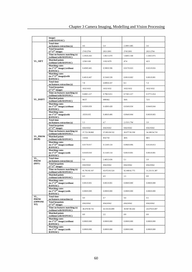
Chapter 3 Camera Imaging, Modelling and Vision Processing
60
image)
(with RANSAC)
VL_SIFT
Total time
on features extraction (s)
4.6
3.4
2.309/1.685
3.6
Total keypoints
(1st/2nd image)
2745/2704
2021/2001
2745/2001
2021/2704
Time on features matching (s)
(without/with RANSAC) 2.293/6.443 1.061/5.070 1.669/2.168 1.544/2.075
Matched points
(without/with RANSAC) 1258/1100 1192/1079 47/4 42/3
Matching rates
(to 1st/2nd image) (without
RANSAC)
0.458/0.465 0.590/0.596 0.017/0.023 0.021/0.016
Matching rates
(to 1st/2nd image)(with
RANSAC)
0.401/0.407
0.534/0.539
0.001/0.002
0.001/0.001
VL_DSIFT
Total time
on features extraction (s) 7.8 4.009/4.337 8.3 7.4
Total keypoints
(1st/2nd image) 1632/1632 1632/1632 1632/1632 1632/1632
Time on features matching (s)
(without/with RANSAC) 0.608/1.217 0.796/3.011 0.718/1.217 0.577/1.014
Matched points
(without/with RANSAC) 96/57 698/662 56/6 72/5
Matching rates
(to 1st/2nd image) (without
RANSAC)
0.059/0.059 0.428/0.428 0.034/0.034 0.044/0.044
Matching rates
(to 1st/2nd image)(with
RANSAC)
.035/0.035 0.406/0.406 0.004/0.004 0.003/0.003
VL_PHOW
(RGB)
Total time
on features extraction (s)
5.3
4.7
2.153/1.794
3.9
Total keypoints
(1st/2nd image)
6562/6562
6562/6562
6562/6562
6562/6562
Time on features matching (s)
(without/with RANSAC) 37.721/38.860 37.003/38.532 30.077/30.358 34.180/34.710
Matched points
(without/with RANSAC) 110/64 816/750 40/6 88/5
Matching rates
(to 1st/2nd image) (without
RANSAC)
0.017/0.017 0.124/0.124 0.006/0.006 0.013/0.013
Matching rates
(to 1st/2nd image) (with
RANSAC)
0.010/0.010 0.114/0.114 0.001/0.001 0.001/0.001
VL_
PHOW
(HSV)
Total time
on features extraction (s) 5.0 2.465/2.636 5.1 3.9
Total keypoints
(1st/2nd image) 6562/6562 6562/6562 6562/6562 6562/6562
Time on features matching (s)
(without/with RANSAC) 41.761/42.167 43.072/43.524 42.448/42.775 31.231/31.387
Matched points
(without/with RANSAC) 6/3 4/3 1/1 0/0
Matching rates
(to 1st/2nd image) (without
RANSAC)
0.001/0.001 0.001/0.001 0.000/0.000 0.000/0.000
Matching rates
(to 1st/2nd image) (with
RANSAC)
0.000/0.000 0.000/0.000 0.000/0.000 0.000/0.000
VL_
PHOW
(OPPONE
NT)
Total time
on features extraction (s) 4.0 4.7 4.6 4.5
Total keypoints
(1st/2nd image) 6562/6562 6562/6562 6562/6562 6562/6562
Time on features matching (s)
(without/with RANSAC) 38.470/38.735 43.555/43.899 39.967/40.264 24.679/25.007
Matched points
(without/with RANSAC) 0/0 2/2 0/0 0/0
Matching rates
(to 1st/2nd image) (without
RANSAC)
0.000/0.000 0.000/0.000 0.000/0.000 0.000/0.000
Matching rates
(to 1st/2nd image) (with
RANSAC)
0.000/0.000 0.000/0.000 0.000/0.000 0.000/0.000

Chapter 3 Camera Imaging, Modelling and Vision Processing
61
Results in Table 3.6.2 show that good number of features can be extracted from
both visible and infrared images. In most cases, even higher matching rate in infrared
images compared to EO images is obtained. When the number of matched points
increases, RANSAC works effectively for both image types given the number of
rejected false-matches.
ASIFT showed very impressive results regarding the highest number of matched
features and matching rates. However, it’s running time costs more than other
algorithms. This is partly due to the large number of features to be extracted.
As the fastest implementation, for the same band images, SURF has quite similar
matching rates as high as VL_SIFT. The latter had more number of features
extracted and matched.
Matching rates in IR images are generally higher than their EO counterparts with
more matched features obtained in most cases. This means that infrared images can
generate a good number of distinguished features based on SIFT.
As fast version of SIFT, VL_DSIFT did not provide remarkable outcomes in either
speed or matched points except relative good number of matched points on infrared
images. However, its performance can be slightly improved by adjusting the steps in
features extraction, with the price to pay for higher matching computation time. This
may not be accepted in our application.
The performance of visual descriptors based on SIFT were overall poor, except
RGB descriptor which was the only one giving convincing outcomes. None of the
other two algorithms worked well as predicted. Overall all colour based descriptors
were not satisfying with these highly blurred (poor spatial resolution) EO and IR
aerial images in contrary to the conclusion in [97].
The nontrivial matching tests cross EO and IR images would not perform well as
expected with methods enumerated in this research. The different characters of
intensity in both EO and IR bands lead to current matching methods not to be really
valid in finding correct correspondences. Many tentative correspondences were
rejected after applying with RANSAC as matches obtained originally might not be
reliable. To meet the practical request, an alternative effective solution needs to be
looked into in the future.

Chapter 3 Camera Imaging, Modelling and Vision Processing
62
In addition, it was noted that although the same matching methodology was
adopted for all algorithms, the matching time may not be comparable as it largely relies
on the number of features extracted. Practically, the trade-off between the number of
features to be extracted and matching time should be taken into account. Subject to the
current matching method utilised in this research, the rest of the tests were conducted
only between images of EO-EO and IR-IR bands.
3.6.4 Comprehensive Tests on Images in Different Environment
These tests were based on the images taken in different environments, i.e., rural
and urban area. We aim to look into the performance of variants of SIFT in different
nature of images in various environments. These environments offer different
challenges with rural image sequences (VI/IR 2&3) appearing quite uniform with
minimal landmarks in comparison to that (VI/IR 32&33) of urban areas, as shown in
Figure 3.6.11. Both the visible and infrared image sequences were re-sampled using 10
frames (0.4s) interval from the video of 25 frames per second. These images were
provided by the industrial partner (MBDA).The test results are presented in Table 3.6.3.
VI 2.JPG VI 3.JPG IR 2.JPG IR 3.JPG
VI 32.JPG VI 33.JPG IR 32.JPG IR 33.JPG
Figure 3.6.11 Visible (LHS: two columns) and Corresponding Infrared images
(RHS: two columns)
Table 3.6.3 Features Extraction and Matching from images in different Environments
Images/Extraction &
Matching
Algorithms/Sections
Rural EO:
VI 2.JPG - VI 3.JPG
Rural IR:
IR 2.JPG - IR 3.JPG Urban EO:
VI 32.JPG - VI 33.JPG
Urban IR:
IR 32.JPG - IR
33.JPG
ASIFT
Total time
on features extraction (s)
14.0
13.0
17.0
15.0
Total keypoints
(1st/2nd image)
1540/1599
3600/1530
20225/19919
16984/15297
Time on features matching (s)
(without/with RANSAC) 0.712/2.723 0.801/1.723 75.697/88. 988 0.764/2.777
Matched points
(without/with RANSAC) 720/477 538/229 8894/6742 8821/6936
Matching rates
(to 1st/2nd image) (without
RANSAC)
0.468/0.450 0.149/0.352 0.440/0.447 0.519/0.577

Chapter 3 Camera Imaging, Modelling and Vision Processing
63
Matching rates
(to 1st/2nd image) (with
RANSAC)
0.310/0.298 0.064/0.150 0.333/0.338 0.408/0.453
SURF
Total time
on features extraction (s) 0.6 0.5 1.0 1.0
Total keypoints
(1st/2nd image) 19/28 68/20 901/1038 530/481
Time on features matching (s)
(without/with RANSAC) 0.000/0.468 0.000/0.359 0.109/1.108 0.047/1.186
Matched points
(without/with RANSAC) 14/7 20/6 309/192 268/183
Matching rates
(to 1st/2nd image) (without
RANSAC)
0.737/0.500 0.294/1.000 0.343/0.298 0.506/0.557
Matching rates
(to 1st/2nd image) (with
RANSAC)
0.368/0.250 0.088/0.300 0.213/0.185 0.345/0.380
VL_SIFT
Total time
on features extraction (s) 3.9 3.4 3.6 3.2
Total keypoints
(1st/2nd image) 2437/2447 1972/1973 2010/1957 1466/1533
Time on features matching (s)
(without/with RANSAC) 1.264/2.168 1.201/1.919 1.186/2.808 0.702/2.200
Matched points
(without/with RANSAC) 198/96 113/36 475/278 433/290
Matching rates
(to 1st/2nd image) (without
RANSAC)
0.081/0.081 0.057/0.057 0.236/0.243 0.295/0.282
Matching rates
(to 1st/2nd image) (with
RANSAC)
0.039/0.039 0.018/0.018 0.138/0.142 0.198/0.189
VL_DSIFT
Total time
on features extraction (s) 11.4 13.4 12.2 12.0
Total keypoints
(1st/2nd image) 1715/1715 1776/1776 1715/1715 1776/1776
Time on features matching (s)
(without/with RANSAC) 0.562/1.061 0.967/1.529 0.749/2.153 0.874/2.028
Matched points
(without/with RANSAC) 152/49 68/16 486/220 308/124
Matching rates
(to 1st/2nd image) (without
RANSAC)
0.089/0.089 0.038/0.038 0.283/0.283 0.173/0.173
Matching rates
(to 1st/2nd image) (with
RANSAC)
0.029/0.029 0.009/0.009 0.128/0.128 0.070/0.070
VL_PHOW
(RGB)
Total time
on features extraction (s) 5.4 5.5 5.6 5.7
Total keypoints
(1st/2nd image) 6909/6909 7045/7045 6909/6909 7045/7045
Time on features matching (s)
(without/with RANSAC) 44.913/45.303 45.131/45.583 46.707/48.314 45.537/46.925
Matched points
(without/with RANSAC) 26/16 25/15 482/257 394/178
Matching rates
(to 1st/2nd image) (without
RANSAC)
0.004/0.004 0.004/0.004 0.070/0.070 0.056/0.056
Matching rates
(to 1st/2nd image) (with
RANSAC)
0.002/0.002 0.002/0.002 0.037/0.037 0.025/0.025
VL_
PHOW
(HSV)
Total time
on features extraction (s) 4.6 6.2 5.7 4.8
Total keypoints
(1st/2nd image) 6909/6909 7045/7045 6909/6909 7045/7045
Time on features matching (s)
(without/with RANSAC) 40.482/40.747 40.342/40.701 47.799/48.267 48.423/49.702
Matched points
(without/with RANSAC) 13/4 26/18 31/23 310/177
Matching rates
(to 1st/2nd image) (without
RANSAC)
0.002/0.002 0.004/0.004 0.004/0.004 0.044/0.044
Matching rates
(to 1st/2nd image) (with
RANSAC)
0.001/0.001 0.003/0.003 0.003/0.003 0.025/0.025
VL_
PHOW
Total time
on features extraction (s) 4.7 6.8 5.0 5.2

Chapter 3 Camera Imaging, Modelling and Vision Processing
64
(OPPONE
NT)
Total keypoints
(1st/2nd image) 6909/6909 7045/7045 6909/6909 7045/7045
Time on features matching (s)
(without/with RANSAC) 37.846/38.049 45.443/45.755 42.885/43.306 27.799/27.955
Matched points
(without/with RANSAC) 0/0 0/0 9/4 0/0
Matching rates
(to 1st/2nd image) (without
RANSAC)
0.000/0.000 0.000/0.000 0.001/0.001 0.000/0.000
Matching rates
(to 1st/2nd image) (with
RANSAC)
0.000/0.000 0.000/0.000 0.001/0.001 0.000/0.000
Table 3.6.3 details the results obtained for this experiment. The following analysis
for these results is given:
More features obtained were from urban images (VI/IR 32&33) than the rural ones
(VI/IR 2&3). Same with matched points as there are more contrast changes with
more distinctive landmarks such as buildings and trees, etc., in the urban area than
the rural area. These results look reasonable.
The consistency of performance is noticed for the first three algorithms, where
SURF was quicker and generated slightly higher matching rates in urban area.
However, less number of extracted and matched points available from all areas are
obtained. Comparing with other algorithms, the matched points in urban area from
SURF may not be good enough to meet real time application.
Again, ASIFT was outstanding compared to the others in terms of number of
features extracted, matched and matching rates. However, computation time was the
highest.
Overall, the standard VL_SIFT was in third place in terms of the above criteria. It
can be a strong competitor for visual navigation taking account the number of
matches and running time. It outperformed VL_DSIFT which achieved reasonable
matched features and rates, but ran slower.
VL_PHOW (RGB) can work better in features rich rural area. The matched points
and rates are acceptable, and it is the best among those colour based SIFTs.
However, its overall rank is still second to non-visual descriptor of SIFT under the
aerial images. Other colour descriptor based SIFTs failed to show the convincing
performance again.
Once more, IR image can provide even higher matching rates (in the case of urban
images) than its visible counterpart.

Chapter 3 Camera Imaging, Modelling and Vision Processing
65
RANSAC played an effective role in eliminating false matches. Wrong matches
could still be present if a large number of features were extracted without
optimisation of the feature detector parameters.
It can be seen that, the studies here show consistency with initial tests under these
specific aerial images. The most convincing results were obtained by ASIFT, SURF and
VL_SIFT. Therefore, the research next will only focus on those more convincing
methods including VL_DSIFT and VL_PHOW (RGB) which is actually the
combination of VL_DSIFT with RGB colour descriptor.
3.6.5 Test for Feature Invariance
This experiment aimed to test the invariance of SIFT variants by changing image
sampling rates. In this scenario, large scene changes via successive images were
induced.
The images used in this test come from the same sequences as the above taken in
rural area, where relatively less number of distinctive landmarks exist. The discrete
image sequences are acquired with sampling rates of 0.2s from the video of 25 frames
per second. Image sequences considered (visible and infrared) in this experiment
contains 10 sampled images. Tests were carried out by comparing between 1st
image
and the other 9 images. Images paired up at different frames can reflect the change of
deformation, illumination and blur. With those images pairs, the feature invariance will
be investigated through the incremental interval of image sampling. The latter is not
only able to verify the effectiveness of feature extraction algorithms but also a useful
reference for real time processing in determining sampling rates for visual navigation.
Parameter settings for dense SIFTs are the trade-off between matching rate and
maximum number of extracted features for the tested images. This is the most important
criteria in our research as it largely determines the number of matched features needed
and related real time consuming. This sub-optimisation setting is utilised for the
parameter suitability among the whole image sequences and to provide a fair
comparison among various feature extraction methods.
Images used in this test are shown in Figure 3.6.12-13 including both visible and
infrared bands. Table 3.6.4 gives overviews of performance for various algorithms. The

Chapter 3 Camera Imaging, Modelling and Vision Processing
66
types of images were represented by only two pairs of images (image 1 and image 2,
image 1 and image 10).
The complete performance in terms of matched features and matching rates for
the whole image sequence are presented in Figure 3.6.14-19.
Figure 3.6.12 Visible images taken from MBDA TV with re-sample rate 0.2s (5 sample interval).
VI 1.JPG
VI 2.JPG
VI 3.JPG
VI 4.JPG
VI 5.JPG
VI 6.JPG
VI 7.JPG
VI 8.JPG
VI 9.JPG
VI 10.JPG
Figure 3.6.12 Visible images taken from MBDA TV(0.2s)
Figure 3.6.13 Infrared images taken from MBDA TV with re-sample rate 0.2s (5 sample interval).
IR 1.JPG
IR 2.JPG
IR 3.JPG
IR 4.JPG
IR 5.JPG
IR 6.JPG
IR 7.JPG
IR 8.JPG
IR 9.JPG
IR 10.JPG
Figure 3.6.13 Infrared images taken from MBDA TV (0.2s)
Table 3.6.4 Overview of Invariance comparison for Feature Extraction and Matching from Visible
and Infrared Images
Images/Extraction &
Matching
Algorithms/Sections
EO (0.2s) :
VI 1.JPG -VI 2.JPG
EO (0.2s) :
VI 1.JPG -VI10.JPG IR (0.2s) :
IR 1.JPG -IR 2.JPG
IR (0.2s) :
IR 1.JPG -IR 10.JPG
ASIFT
Total time
on features extraction (s)
13.0
14.0
14.0
14.0
Total keypoints
(1st/2nd image)
1570/1596
1570/2637
3660/2916
3660/1473
Time on features matching (s)
(without/with RANSAC) 0.733/3.073 0.593/0.827 4.009/8.362 1.700/2.465
Matched points
(without/with RANSAC) 882/624 54/4 1186/748 145/13
Matching rates
(to 1st/2nd image) (without
RANSAC)
0.562/0.553 0.034/0.020 0.324/0.407 0.040/0.098
Matching rates
(to 1st/2nd image) (with
RANSAC)
0.397/0.391 0.003/0.002 0.204/0.257 0.004/0.009
SURF
Total time
on features extraction (s) 0.6 0.6 0.7 0.7
Total keypoints 20/17 20/50 57/56 57/24
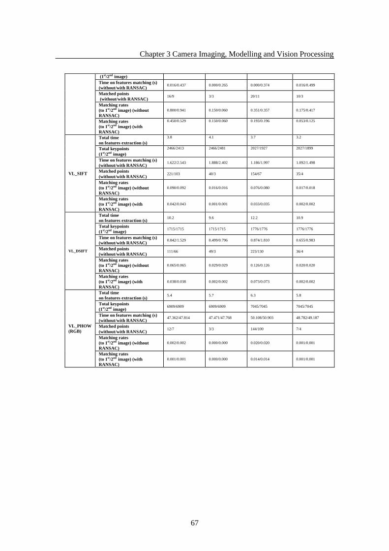
Chapter 3 Camera Imaging, Modelling and Vision Processing
67
(1st/2nd image)
Time on features matching (s)
(without/with RANSAC) 0.016/0.437 0.000/0.265 0.000/0.374 0.016/0.499
Matched points
(without/with RANSAC) 16/9 3/3 20/11 10/3
Matching rates
(to 1st/2nd image) (without
RANSAC)
0.800/0.941 0.150/0.060 0.351/0.357 0.175/0.417
Matching rates
(to 1st/2nd image) (with
RANSAC)
0.450/0.529 0.150/0.060 0.193/0.196 0.053/0.125
VL_SIFT
Total time
on features extraction (s)
3.8 4.1 3.7 3.2
Total keypoints
(1st/2nd image)
2466/2413 2466/2481 2027/1927 2027/1899
Time on features matching (s)
(without/with RANSAC) 1.622/2.543 1.888/2.402 1.186/1.997 1.092/1.498
Matched points
(without/with RANSAC) 221/103 40/3 154/67 35/4
Matching rates
(to 1st/2nd image) (without
RANSAC)
0.090/0.092 0.016/0.016 0.076/0.080 0.017/0.018
Matching rates
(to 1st/2nd image) (with
RANSAC)
0.042/0.043 0.001/0.001 0.033/0.035 0.002/0.002
VL_DSIFT
Total time
on features extraction (s) 10.2 9.6 12.2 10.9
Total keypoints
(1st/2nd image) 1715/1715 1715/1715 1776/1776 1776/1776
Time on features matching (s)
(without/with RANSAC) 0.842/1.529 0.499/0.796 0.874/1.810 0.655/0.983
Matched points
(without/with RANSAC) 111/66 49/3 223/130 36/4
Matching rates
(to 1st/2nd image) (without
RANSAC)
0.065/0.065 0.029/0.029 0.126/0.126 0.020/0.020
Matching rates
(to 1st/2nd image) (with
RANSAC)
0.038/0.038 0.002/0.002 0.073/0.073 0.002/0.002
VL_PHOW
(RGB)
Total time
on features extraction (s) 5.4 5.7 6.3 5.8
Total keypoints
(1st/2nd image) 6909/6909 6909/6909 7045/7045 7045/7045
Time on features matching (s)
(without/with RANSAC) 47.362/47.814 47.471/47.768 50.108/50.903 48.782/49.187
Matched points
(without/with RANSAC) 12/7 3/3 144/100 7/4
Matching rates
(to 1st/2nd image) (without
RANSAC)
0.002/0.002 0.000/0.000 0.020/0.020 0.001/0.001
Matching rates
(to 1st/2nd image) (with
RANSAC)
0.001/0.001 0.000/0.000 0.014/0.014 0.001/0.001

Chapter 3 Camera Imaging, Modelling and Vision Processing
68
Figure 3.6.14 Matched Features from visible
images with 0.2s sample rate(top: without
RANSAC, bottom: with RANSAC)
Figure 3.6.15 Matched Features from infrared
images with 0.2s sample rate(top: without
RANSAC, bottom: with RANSAC)
Figure 3.6.16a Matching rates (MR) (to 1st
image) for EO images with 0.2s sample rate
(without RANSAC)
Figure 3.6.17a Matching rates (MR) (to 1st
image) for IR images with 0.2s sample rate
(without RANSAC)
1 2 3 4 5 6 7 8 90
100
200
300
400
500
600
700
800
900Matched Features without RANSAC
Image frames
Num
ber
of
featu
res m
atc
hed
MF-ASIFT
MF-SURF
MF-VLSIFT
MF-VLDSIFT
MF-VLPHOW(RGB)
1 2 3 4 5 6 7 8 90
200
400
600
800
1000
1200Matched Features without RANSAC
Image frames
Num
ber
of
featu
res m
atc
hed
MF-ASIFT
MF-SURF
MF-VLSIFT
MF-VLDSIFT
MF-VLPHOW(RGB)
1 2 3 4 5 6 7 8 90
100
200
300
400
500
600
700Matched Features with RANSAC
Image frames
Num
ber
of
featu
res m
atc
hed
MF-ASIFT
MF-SURF
MF-VLSIFT
MF-VLDSIFT
MF-VLPHOW(RGB)
1 2 3 4 5 6 7 8 90
100
200
300
400
500
600
700
800Matched Features with RANSAC
Image frames
Num
ber
of
featu
res m
atc
hed
MF-ASIFT
MF-SURF
MF-VLSIFT
MF-VLDSIFT
MF-VLPHOW(RGB)
1 2 3 4 5 6 7 8 90
0.5
1MR-image1 by ASIFT without RANSAC
1 2 3 4 5 6 7 8 90
0.5
1MR-image1 by SURF without RANSAC
1 2 3 4 5 6 7 8 90
0.05
0.1MR-image1 by VLSIFT without RANSAC
1 2 3 4 5 6 7 8 90
0.05
0.1MR-image1 by VLDSIFT without RANSAC
1 2 3 4 5 6 7 8 90
0.005
0.01MR-image1 by VLPHOW(RGB) without RANSAC
1 2 3 4 5 6 7 8 90
0.2
0.4MR-image1 by ASIFT without RANSAC
1 2 3 4 5 6 7 8 90
0.5
1MR-image1 by SURF without RANSAC
1 2 3 4 5 6 7 8 90
0.05
0.1MR-image1 by VLSIFT without RANSAC
1 2 3 4 5 6 7 8 90
0.1
0.2MR-image1 by VLDSIFT without RANSAC
1 2 3 4 5 6 7 8 90
0.01
0.02MR-image1 by VLPHOW(RGB) without RANSAC

Chapter 3 Camera Imaging, Modelling and Vision Processing
69
Figure 3.6.16b Matching rates (MR) (to 2nd
image) for EO images with 0.2s sample rate
(without RANSAC)
Figure 3.6.17b Matching rates (MR) (to 2nd
image) for IR images with 0.2s sample rate
(without RANSAC)
Figure 3.6.18a Matching rates (MR) (to 1st
image) for EO images with 0.2s sample rate
(with RANSAC)
Figure 3.6.19a Matching rates (MR) (to 1st
image) for IR images with 0.2s sample rate
(with RANSAC)
Figure 3.6.18b Matching rates (MR) (to 2nd
image) for EO images with 0.2s sample rate
(with RANSAC)
Figure 3.6.19b Matching rates (MR) (to 2nd
image) for IR images with 0.2s sample rate
(with RANSAC)
1 2 3 4 5 6 7 8 90
0.5
1MR-image2 by ASIFT without RANSAC
1 2 3 4 5 6 7 8 90
0.5
1MR-image2 by SURF without RANSAC
1 2 3 4 5 6 7 8 90
0.05
0.1MR-image2 by VLSIFT without RANSAC
1 2 3 4 5 6 7 8 90
0.05
0.1MR-image2 by VLDSIFT without RANSAC
1 2 3 4 5 6 7 8 90
0.005
0.01MR-image2 by VLPHOW(RGB) without RANSAC
1 2 3 4 5 6 7 8 90
0.5MR-image2 by ASIFT without RANSAC
1 2 3 4 5 6 7 8 90
5
10MR-image2 by SURF without RANSAC
1 2 3 4 5 6 7 8 90
0.05
0.1MR-image2 by VLSIFT without RANSAC
1 2 3 4 5 6 7 8 90
0.1
0.2MR-image2 by VLDSIFT without RANSAC
1 2 3 4 5 6 7 8 90
0.01
0.02MR-image2 by VLPHOW(RGB) without RANSAC
1 2 3 4 5 6 7 8 90
0.5MR-image1 by ASIFT with RANSAC
1 2 3 4 5 6 7 8 90
0.5MR-image1 by SURF with RANSAC
1 2 3 4 5 6 7 8 90
0.05MR-image1 by VLSIFT with RANSAC
1 2 3 4 5 6 7 8 90
0.020.04
MR-image1 by VLDSIFT with RANSAC
1 2 3 4 5 6 7 8 90
2
4x 10
-3 MR-image1 by VLPHOW(RGB) with RANSAC
1 2 3 4 5 6 7 8 90
0.1
0.2MR-image1 by ASIFT with RANSAC
1 2 3 4 5 6 7 8 90
0.2
0.4MR-image1 by SURF with RANSAC
1 2 3 4 5 6 7 8 90
0.02
0.04MR-image1 by VLSIFT with RANSAC
1 2 3 4 5 6 7 8 90
0.05
0.1MR-image1 by VLDSIFT with RANSAC
1 2 3 4 5 6 7 8 90
0.01
0.02MR-image1 by VLPHOW(RGB) with RANSAC
1 2 3 4 5 6 7 8 90
0.5MR-image2 by ASIFT with RANSAC
1 2 3 4 5 6 7 8 90
0.51
MR-image2 by SURF with RANSAC
1 2 3 4 5 6 7 8 90
0.05MR-image2 by VLSIFT with RANSAC
1 2 3 4 5 6 7 8 90
0.020.04
MR-image2 by VLDSIFT with RANSAC
1 2 3 4 5 6 7 8 90
2
4x 10
-3 MR-image2 by VLPHOW(RGB) with RANSAC
1 2 3 4 5 6 7 8 90
0.2
0.4MR-image2 by ASIFT with RANSAC
1 2 3 4 5 6 7 8 90
2
4MR-image2 by SURF with RANSAC
1 2 3 4 5 6 7 8 90
0.02
0.04MR-image2 by VLSIFT with RANSAC
1 2 3 4 5 6 7 8 90
0.05
0.1MR-image2 by VLDSIFT with RANSAC
1 2 3 4 5 6 7 8 90
0.01
0.02MR-image2 by VLPHOW(RGB) with RANSAC

Chapter 3 Camera Imaging, Modelling and Vision Processing
70
In the above table and graphs, we can see that individual performance of
algorithms on matched numbers has quite similar trends from EO to IR images as
shown in Figure 3.6.14-19. The number of matched features in descending order was
obtained by ASIFT, VL_SIFT, VL_DSIFT, VL_PHOW (RGB) and SURF respectively.
In Table 3.6.4 and Figure 3.6.14-19, the number of matched features and
matching rates are both decreasing with increase of interval time. Generally, the 1st, 2
nd,
and 3rd
image pairs can have more common features. The rest are unsoundness and the
overall performance on matching rates after 3rd
frame is rather poor. As the number of
features obtained in rural images is naturally less than images, this further degenerate
the matching performance when the sampling rates dropped down. Overall the
performance of the first three methods in the table can utilise more frames and hence
permit more viewpoint changes in the image sequence.
SIFT and ASIFT have the largest number of matched keypoints. SURF is still less
time consuming with quite similar matching rates as ASIFT. There was a little bit of
uneven stability for its performance in IR images.
Once again, there was an intuitive impression of increasing matched points and
matching rates obtained in infrared images. The even more convincing pattern
illustrating such trends was obtained by VL_DSIFT and VL_PHOW (RGB). This
further proved that infrared images can indeed provide good number features for
matching. It also can be seen in this test that the application of RANSAC helped to
remove outliers, and generally matching accuracy can be improved as well.
Through this experiment conducted on images from a specific environment, the
overall first three algorithms (SIFT, ASIFT, SURF) are indeed convincing. This
provides good candidates to select in our application real-world visual navigation
problem.
3.7 Summary and Discussion
In this chapter, the concept and theory background regarding imaging and vision
processing related to our project was presented. This includes camera imaging,
modelling, calibration and epipolar geometry.

Chapter 3 Camera Imaging, Modelling and Vision Processing
71
The focus was down to image processing algorithms and techniques - variants of
SIFT. A number of experiments were conducted in order to have in-depth insights into
various aerial images. This covered both visible and infrared images with successful
utilisation of various SIFT algorithms.
This comprehensive analysis of both visible and infrared images with variants of
SIFT is novel, and up to the reviewed literatures, no such research was ever conducted.
Current aerial visual navigation and mapping requirements spurred us to carry out these
studies. We have concluded the findings below.
It is usually known that SIFT provides more features and slightly better feature
descriptors for matching. Among variants of SIFT, ASIFT outperforms the others in
terms of matched points and rates. SURF is generally intended to speed up the process
and provides higher matching rates for both visible and infrared image sequences.
However, the matching points are somehow below the expectation for our application in
certain cases.
Most of the methods adopted in this research can work well on infrared images.
We believe that infrared images can provide good number of matched points with
matching rate in some cases even higher than that of visible counterparts for certain
methods. It is the significative investigation that there is feasibility to have reliable
matches for the purpose of application with cross image bands given appropriate
matching methods. Overall, it is encouraging that infrared images can provide robust
and effective matches with usual feature extraction methods to meet the challenges of
visual navigation and mapping tasks. All these are, of course, subject to appropriate
sampling intervals that are determined by the stereo rig and image processor on board.
The application of RANSAC algorithm can remove false feature matches
effectively. This has been proved to be a useful technique in refining the matches and it
was utilised well in feature matching for this research. However, its mechanism can
prevent its effectiveness in the presence of large numbers of outliers in data set. This
will be the motivation to our research on effective methods for descriptor based
matching problems.

Chapter 4 Data Filtering and Estimation Analysis in vSLAM
72
CHAPTER 4
Data Filtering and Estimation Analysis in vSLAM
In this chapter, the theory and algorithm of several novel filters are presented. The
process model for air vehicle and stereo vision based camera observation model were
fitted for those filters. A comprehensive analysis was drawn from the experiments of
these filtering methods utilised with vSLAM.
4.1 Introduction
In recent years, sensing and computing technology in both the research and
application domains has made tremendous progress. Rewarded by those advancements,
the original concepts of SLAM [1, 2] has been extended and many special cases have
arisen [111-113] since then. Some of them can be classified with the various sensors
and different filters categories. The former are based on range-bearing of Laser, Radar,
Sonar, digital camera …, etc., while the latter adopted Extended KF/IF, UKF, H
infinity, Particle Filters…, etc. Among those, passive camera based SLAM, named as
visual SLAM, refers to the information from images as the sole external sensor data.
Although SLAM has been widely studied by the robotics and the computer vision
communities in past decades, visual SLAM is still an active area for researchers due to
the advantages of low cost cameras in providing flexible, enriched information for
visual navigation. The use of cameras as sensing devices on robots allows the
development of accurate autonomous systems meanwhile decreasing costs and overall
energy consumption.
The fundamental principle of SLAM was derived from Bayesian framework.
Being the primitive mechanism, state estimation can be regarded as an objective cost
function for optimisation in EKF-SLAM (Durrant-Whyte & Bailey, 2006) [108].
However, the inherent drawback from truncation of Tailor series leads to EKF-SLAM's
failure in large environments caused by the problem of the linearisation process (this
can results in inconsistent estimation) (Rodriguez-Losada et al., 2006) (Bailey et al.,
2006) (Shoudong & Gamini, 2007), [53, 109, 110] especially when high nonlinearity
system models are adopted.

Chapter 4 Data Filtering and Estimation Analysis in vSLAM
73
Therefore, the accuracy and robustness of estimation for SLAM have been
attracting significant efforts from researchers since the establishment of EKF-SLAM. It
is common sense that data fusing is the indispensable part of the SLAM. Extended
Kalman filter (EKF) [4] has been the conventional filter employed with SLAM. It is a
convenient with feasible implementation. Its first-order linearisation as an
approximation to the optimal solution, the nonlinear function, the substantial errors will
be introduced in the estimates of true posterior mean and covariance of the transformed
distribution. Sometime this may lead to the divergence of the filter. This is the inherent
reason of sub-optimal performance and even divergence of the EKF resulted from high
nonlinear system, such as vSLAM incorporated with UAV. Therefore, those errors
caused by linearisation may yield to an inconsistent map [34].
Although there are various filtering algorithms available in data fusion [4], such
as particle filters which has impressive performance in many areas. However, the high
computation cost is generally a bottleneck [4] of its implementation in highly
dimensional, complex and nonlinear system, e.g. 6 DoF vSLAM for UAVs. We usually
need to have the trade-offs in computation efforts and high performance. Therefore, a
few carefully selected alternatives were investigated in this research.
Unscented Kalman filter (UKF) which has some similar features as particle filter
[4] is one of those alternatives for EKF. It addresses the approximation issues of the
EKF and the linearity assumptions of the KF. Same as EKF, in the UKF the state
distribution is again represented by a Gaussian Random Variable (GRV). It is
understood that Unscented transform (UT) uses a minimal set of deterministically
chosen sample points to approximate a probability distribution [33, 35, 36]. These
sample points completely capture the true mean and covariance of the GRV and are then
propagated through the true nonlinear system. This allows estimation of the posterior
mean and covariance to the third order for any nonlinearity. This distinctive
characteristic of the UT has attracted interest of scholars for the purpose of
incorporation in high nonlinear system.
The Unscented Kalman Filter (UKF) adopts the UT for the transformations
required by the Kalman filter. In linear models, UKF is equivalent to the KF with
similar computational complexity. However, it is theoretically more accurate for

Chapter 4 Data Filtering and Estimation Analysis in vSLAM
74
nonlinear system and can provide better fusing data by tuning parameters setting with
sigma points in best approximation to the true distribution. It also does not require the
derivation of any Jacobians.
There have been some successful applications in ground robots with UKF [31].
Occasional examples in UAV where DoF is high [32] under specific sensing system in
either range bearing, or monocular vision system on board are noticed.
There is a factor to be aware of when utilising the Cholesky decomposition with
UT. Apart from its inherently heavy computational demands, it is known that the
numerically unstable matrix operation normally tends to cause the covariance matrix to
be a negative definite. Therefore, it is hard to meet the conditions demanded by
successful conduction of a Cholesky decomposition on a high dimension matrix. This
generally occurs in a high nonlinear system such as UAV with vSLAM, which yields to
the failure when carrying out UT in the standard way. The alternative approximated
methods like SVD decomposition brings in errors when it is used to obtain UT.
UKF is the combination of UT and Kalman filter in the correction stage. Usually,
this defect cannot be overcome by simply updating with the observation.
Recent years, H∞ filters have received considerable attention [4]. In contrast to
the conventional Kalman filter that requires an exact and accurate system model as well
as perfect knowledge of the noise statistics, H∞ filter requires no prior knowledge of the
noise statistics but finite bounded energies. In particular, unlike Kalman filter that aims
to give the minimum mean-square estimate, the optimal H∞ filter tries to minimise the
effect of the worst possible disturbances on the estimation errors, Hence, it is more
robust against model uncertainty [4]. Taking this merit, incorporating unscented
transform in H∞ to obtain a different data fusing technique for the navigation of UAV
with vSLAM is certainly worth attempting. In our experiments, this was conducted by
the comparison of Unscented Transform H∞ (UHF) and other filters, which is one of
objectives in this thesis [37, 38].
In addition to the theoretical maturity of single vehicle SLAM [1, 2, 28], one of
the research agendas for SLAM has been directed to multi-vehicles or multi-sensors
SLAM. Because of the distribution of the co-operative vehicles, to deal with the process
or the observation information from the environment, and to estimate the specific states
Chapter 4 Data Filtering and Estimation Analysis in vSLAM
75
of interest by relating these observations to the states through the process or
environment models, data-fusing algorithms become the considerable aspect to be re-
investigated for the sake of efficiency and accuracy. The active research has focus on
this area for many years. For SLAM, Extended Kalman Filter (EKF)[4] is still a
valuable and a feasible implementation, but another alternative - Information Filter most
likely can bring more benefits as its correction form makes it more suitable for multi-
sensors data fusion.
The Information Filter (IF) is utilised by propagating the inverse of the state error
covariance matrix. Its theoretical advantages over the Kalman filter can be summarised
[111] as follows: the more accurate estimates can be obtained through simply summing
the information matrices and vector [114]. It is generally more stable than KF [115] and
relatively quicker in estimating high dimensional maps [116]. This is because updates
can be batch processed in IF, while KF needs to individually deal with the effects to all
Gaussian parameters by single measurement which is time consuming when handling
rich landmarks environments.
However, the recovery of states estimate in both prediction and update steps when
needed are the primary disadvantage of IF in nonlinear systems. This step requires the
inversion of the information matrix. In high dimensional state spaces, computation cost
can be normally be the main limitation to be utilised comparing with the Kalman filter.
There are some contributions to solve this problem by using sparse extended
information filter [114, 116], where the information matrix is approximately sparse, and
developed extended information filter is significantly more efficient than conventional
KF and IF. As in most robotics problems, the local interaction of state variables results
the sparse information matrix, where states are connected only when the corresponding
off-diagonal element in the information matrix is non-zero. There are some successful
algorithms to give the efficient updating and estimation performance [117, 118].
To verify the effectiveness of EIF with current and forthcoming application in
cooperative vSLAM (C-vSLAM), we conducted an investigation of the standard
Extended Information Filter (EIF) [7]. Comparing with EKF in terms of accuracy and
robustness for single UAV vSLAM will help in the selection of the suitable filter later
on for co-operative vSLAM.

Chapter 4 Data Filtering and Estimation Analysis in vSLAM
76
The external sensors for vSLAM are the binocular vision system to obtain space
coordinates of the landmarks drawn from computer vision. This makes the feature
extraction methods play an important role in providing high quality perception to UAVs
all through this mission.
Scale Invariant Feature Transform (SIFT) [12], and Speeded-Up Robust Features
(SURF) [17] are utilized in our vSLAM experiment. SIFT presented by Lowe, apart
from the success in application with many images processing area such as image
mosaic, recognition, retrieval, has also been successfully applied to vSLAM [40]. SURF
is presented by Bay and al, which is regarded as a faster method with good a quality of
feature extraction to theoretically meet the real time requirement. We, therefore, test
their performance by utilising both of them in vSLAM to have convincing performance
for this project.
In next sections, several comparisons among data filters of EKF, UKF, UHF and
EIF under different noise settings were conducted comprehensively with the above
features extraction methods.
4.2 Extended Kalman Filter
As one of the main paradigms in SLAM, EKF has been widely used for nonlinear
system, but it is using the approximation of 1st order Taylor extension. This is later the
fountainhead of estimation errors and the Jacob matrix calculation is the big burden for
high nonlinear system like vSLAM for UAV. Nevertheless, EKF is still the priority
choice in vSLAM and the following steps present the implementation of EKF as an
iterative prediction-sense-update process with its widely known formulation:
Prediction
(4.2.1)
Observation
)(,,1 kwkukxFkxe
)(, kvkxHkz ee
)()(1 kJkQkJkJkPkJkP T
FwFw
T
FxFxe
kzkzki em )(

Chapter 4 Data Filtering and Estimation Analysis in vSLAM
77
(4.2.2)
Update
(4.2.3)
where Jacob matrixes are denoted as
where F(:) and H(:) are processing and measurement model respectively, which are
described by INS [40] and the projection or landmarks from world frame to camera
coordinates [40] ,which will be explained later.
4.3 Unscented Kalman Filter
4.3.1 Unscented Transform (UT) Technique
The UT is a method to calculate the statistics of a random variable that undergoes
a nonlinear transformation [33]. To carry out unscented transform, under certain state
distribution assumption, we suppose that an L dimensional random vector, having a
mean and a covariance propagates through an arbitrary nonlinear function.
The unscented transform creates 2L+1 sigma vectors and weights W. These sigma
points can completely capture the true mean and covariance of the supposed pdf
(probability of distribution function) of random variable. With propagation of these
sigma points through the true non-linear system, the captured posterior mean and
covariance are accurate up to the 3rd order Taylor series expansion [33].
Considering propagating a random variable X (dimension L) through a discrete
time nonlinear transition equation
kkk wxFxequationState )(: 1
kkk vxHyequationtMeasuremen )(: 11
(4.2.4)
)()()()()( kJkRkJkJkPkJkS T
HxHv
T
HxeHx
kSJkPkK T
Hxe
1)(
kikKkxkx e )(
kKkSkKkPkP T
e )(
,xFJ Fx ,wFJ Fw ,xHJ Hx ,vHJ Hv
)1.3.4(

Chapter 4 Data Filtering and Estimation Analysis in vSLAM
78
where F(x) and H(x) represent system process and observation model respectively. xk is
n-dimensional state of the system and y k is m dimensional observation sequence. w k is
p dimensional process noise sequence. v k is m-dimensional observation noise sequence.
The general procedure in (4.3.2) is used to obtain the unscented transformation.
(4.3.2)
When taken into account of the scaling parameter k, which determines the
approximated accuracy for the order of Taylor series expansion, we have:
(4.3.3)
• is a constant to determine the spread of the sigma points around x and is
usually set to a small positive value (e.g., 4101 ).
• is a secondary scaling constant usually set to 3-L or 0 for a Gaussian.
• The constant is used to incorporate prior knowledge of the distribution of x
(for Gaussian distributions, =2 is optimal).
• ixPL is the i
th column of the matrix square root of xPL .
Through the measurement model H(x), we have observation updating as
(4.3.4)
LL )(2
0
( )
0
( ) ( ) 2
0 0
( )( ) ( ) 0
2
( ) 1,...,
( ) 1,..., 2
( )
(1 )
1,..., 22
( 1)
( )
i i
i i L
m
c m
mm c
i i
i L
i L L
WL
W W
WW W i L
L
L
x
x
x
x P
x P
2( )
0
2( )
0
( ) 0,..., 2
( )( )
i i
i Lm
i i
i
i Lc T
i i i
i
h i L
W
W
y
y
P y y

Chapter 4 Data Filtering and Estimation Analysis in vSLAM
79
4.3.2 Unscented Kalman Filter (UKF)
UKF is a straightforward prediction-sense-update application of the unscented
transformation. It is an extension of UT to the Kalman Filter framework by using UT to
implement the transformations for both time and measurement updating. There is no
need for explicit calculation of Jacobians or Hessians to implement this algorithm. This
is the most important advantage of the UKF apart from that it addresses the
approximation issues up to 3rd
order of Taylor extension [33] compared to EKF.
Summarisation of UKF is following in the same system model as in the above section.
Initialisation for state mean and covariance:
][ˆ00 XEX , ])ˆ)(ˆ[( 00000
TXXXXEP (4.3.5)
Time update equations:
(4.3.6)
kx : States prediction.
:
kP Predicted state covariance matrix.
ky : Measurement prediction.
Qk : Process noise covariance matrix.
Computed sigma point of states.
Computed sigma point of measurements. The prediction of the state variable (output) at time instant based on the state
variable (input) at time k-1 is denoted by subscript k/k-1.
Measurement update equations:
, 1, 1
2( )
, 10
2( )
, 1 , 10
, 1 , 1
2( )
, 10
( ) 0,1,..., 2
( )( )
i ki k k
Lm
k i i k ki
Lc T
k kk i ki k k i k ki
i k k i k k
Lm
ik i k ki
i L
W
W
W
F
x
P x x Q
H
y
~ ~
~ ~
~ ~ ~ ~
~ ~
2( )
, 1 , 10
2( )
, 1 , 10
1
( )( )
( )( )
( )
k k
k k
k k k k
k k
Lc T
i kk ki k k i k ky y
i
Lc T
ki ki k k i k kx y
i
kx y y y
k k k k k
T
k k k ky y
W
W
K
K y
K K
P y y R
P x y
P P
x x y
P P P
)7.3.4(
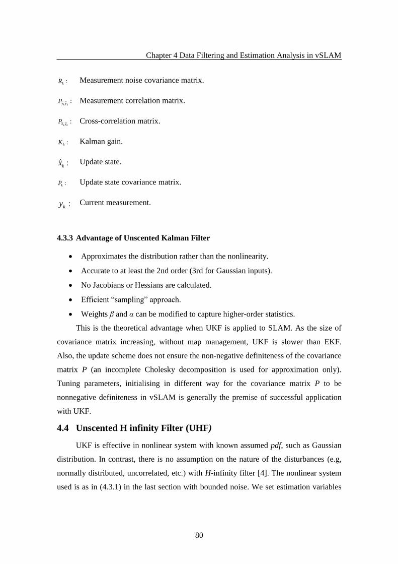
Chapter 4 Data Filtering and Estimation Analysis in vSLAM
80
:kR Measurement noise covariance matrix.
:~~kk yyP Measurement correlation matrix.
:~~kk yxP Cross-correlation matrix.
:kK Kalman gain.
:ˆkx Update state.
:kP Update state covariance matrix.
:ky Current measurement.
4.3.3 Advantage of Unscented Kalman Filter
Approximates the distribution rather than the nonlinearity.
Accurate to at least the 2nd order (3rd for Gaussian inputs).
No Jacobians or Hessians are calculated.
Efficient “sampling” approach.
Weights β and α can be modified to capture higher-order statistics.
This is the theoretical advantage when UKF is applied to SLAM. As the size of
covariance matrix increasing, without map management, UKF is slower than EKF.
Also, the update scheme does not ensure the non-negative definiteness of the covariance
matrix P (an incomplete Cholesky decomposition is used for approximation only).
Tuning parameters, initialising in different way for the covariance matrix P to be
nonnegative definiteness in vSLAM is generally the premise of successful application
with UKF.
4.4 Unscented H infinity Filter (UHF)
UKF is effective in nonlinear system with known assumed pdf, such as Gaussian
distribution. In contrast, there is no assumption on the nature of the disturbances (e.g,
normally distributed, uncorrelated, etc.) with H-infinity filter [4]. The nonlinear system
used is as in (4.3.1) in the last section with bounded noise. We set estimation variables

Chapter 4 Data Filtering and Estimation Analysis in vSLAM
81
kkk xLz , where kL is user-defined matrix ( kL is identity if only the states are estimated).
In the game theory approach for H∞ filtering, the following cost function is defined [4]:
1
0
222
00
1
0
2
10
ˆˆN
kRkQkP
N
kSkk
kkk
vwxxzzJ (4.4.1)
where 0P is positive definite matrix, which reflects a prior knowledge as how close 0x is
to the initial estimate 0x that is a priori estimate of 0x . ke = ( 0x - 0x ) represents
unknown initial estimation error. 2
Wa is the square of weighted 2l norm of a as WaaT .
Q>0 and R>0 are weighting matrices to be determined by the satisfaction performance
requirements. In practical systems, Q and R can be chosen as the estimates of the
covariance matrices of the corresponding noises.
Let )(FTkdenotes the transfer operator mapping the unknown disturbance
kk vwxx ,),ˆ( 00 to filtering error { ke }. The H-infinity norm [37,38] )(FTk is from
disturbance input to the filtering error output:
2,2,
2
0
supinf)(inflvlwxF
kF KK
JFT
(4.4.2)
where γ>0 is a given scalar. The optimal H filter can be obtained to the desired
accuracy by iterating on γ for the suboptimal solution.
The above definitions indicate that, H filter is designed to ensure the minimum
estimation error energy gain induced by all the disturbance importations that having
identified energy [4].
It is noted that, for the nonlinear system, the extended H filter has an observer
structure similar to that of the extended Kalman filter [4, 37, 38]. Q and R play the same
role as the covariance matrices of the process noise and the measurement noise as when
using the extended Kalman filtering. It is more robust than EKF as it does not take any
assumption on noise. Moreover, the extended H filter reduces to the extended Kalman
filter when [4]. Thus, γ may be thought of as a tuning parameter to control the
trade-off between H performance and minimum variance performance.
Incorporating the same merits with unscented transform of UKF [33] results in
sigma point H filter (UHF) [37, 38] which takes the advantages both of unscented

Chapter 4 Data Filtering and Estimation Analysis in vSLAM
82
transform and non-requirement for assumption pdf. From theoretical point of view,
more accuracy estimation should be achieved by UHF filtering.
We take the same process and measurement model as (4.3.1), and approximately
adopting following formula [41] as the replacement of measurement covariance and
corresponding cross-covariance:
T
kkkyy HPHPkk
~~
T
kkkyx HPPk
~~
Instead of using Kalman gain directly, we substitute the state covariance
correction in UKF as follows [37]:
T
kyx
k
T
yx
yx
yy
kyxkk PPIP
P
P
IPPPPP
kk
kk
kk
kk
kk][
)(][ ~~
1
2
~~
~~
~~
~~
(4.4.4)
The value of the tuning parameter is chosen to guarantee the positiveness of
covariance matrix P and control the performance of H filter. For the practical use,
determines the H infinity is sub optimal. It is usually set to smaller value (0<<2) which
indicates the filter with better performance [38].
:~~kk yyP Measurement correlation matrix.
:~~kk yxP Cross-correlation matrix.
:kP Update state covariance matrix.
:
kP Predicted state covariance matrix.
:I Identity matrix.
4.4.1 Advantage of Unscented H Filter
Besides having the same advantages as UKF, there is no constraint to the
assumption of pdf. This is more suitable for the practical application as the noise is
usually uncertain in practical environment.
)3.4.4(

Chapter 4 Data Filtering and Estimation Analysis in vSLAM
83
4.5 Extended Information Filter (EIF)
The information filter is essentially a Kalman filter expressed in terms of
measures of information about the parameters (state) of interest rather than direct state
estimates and their associated covariance [7]. It is also called the inverse covariance
form of the Kalman filter [7]. The system indicated above is having the following EIF
form:
Prediction
))1(),1(),1/1(ˆ,()1/()1/(ˆ kkukkxkFkkYkky (4.5.1)
11 )]()()1/1()([)1/( kQkFkkYkFkkYT
xx (4.5.2)
Estimation
)()1/(ˆ)/(ˆ kikkykky (4.5.3)
)()1/()/( kIkkYkkY (4.5.4)
where, )1/(ˆ),/(ˆ kkykky are information state vector, with information state contribution
)]1/(ˆ)()()[()()( 1 kkxkHkkRkHki x
T
x (4.5.5)
and innovation
))1/(ˆ()()( kkxHkzk (4.5.6)
)1/(),/( kkYkkY are information matrix with
)()()()( 1 kHkRkHkI x
T
x (4.5.7)
where
1)(ˆ)/(ˆ),/(ˆ)/(ˆ)/(ˆ kPkkYkkxkkYkky (4.5.8)
are the connection between EIF and EKF.
The prediction of the state variable (output )/(ˆ kky , )/(ˆ kkY , )/(ˆ kkx , )/(ˆ kkP ) at time
instant k based on the state variable (input )1/(ˆ kky , )1/(ˆ kkY , )1/(ˆ kkx , )1/(ˆ kkP ) at time
k-1 is denoted by subscript k/k-1.
:kY Information matrix.
:ky Information state vector.
:kP State covariance.

Chapter 4 Data Filtering and Estimation Analysis in vSLAM
84
:ˆkx State vector.
:kz Current measurement.
:kQ Processing noise covariance matrix.
:kR Measurement noise covariance matrix.
4.5.1 Advantage of Information Filter
An overall information filter can provide advantages in following aspects.
First of all, estimation equation is computationally simpler than EKF estimation
equation. It is easier to distribute and fuse because of the orthonormality of information
space. Moreover, using the decentralised form of EIF, the observation made by several
sensors at a particular time, can be combined to obtain more accurate estimates. This
can be indicated in below:
Suppose the number of UAVs is M and for the jth UAV where j = 1... M, each
UAV maintains a record of the information sent during the last communication (i.e.,
)1/1(),1/1( kkykkY jj). This is subtracted from the current information to form the
new information that UAV has about the feature map [8]:
)1/1()/()/()(, kkYkkYkkY jjknewj (4.5.9)
)1/1()/()/()(, kkykkykky jjknewj (4.5.10)
This new information will be then transferred among the other UAVs. After each
UAV receives all of the information updated from the other UAVs, these information
are summed together along with the current UAV information to form the updated
estimation of the UAV location and map features in information form:
)/()/()/(
1
,)(, kkYkkYkkYM
j
newjjkupdatej
)/()/()/(
1
,)(, kkykkykkyM
j
newjjkupdatej
)11.5.4(

Chapter 4 Data Filtering and Estimation Analysis in vSLAM
85
Once all of the information from other UAVs is combined in the update, a state
space estimate of the map feature locations and covariance can be recovered back into
the states in EKF using equation as definition:
1)/(ˆ)(ˆ),/(ˆ)/(ˆ)/(ˆ kkYkPkkykkPkkx (4.5.12)
EIF still has the drawbacks inherent in EKF. However, the updating form of EIF
is more suitable for multi-sensor cooperative system. With the experiment carried out
next, the filtering accuracy in EIF is quite similar to EKF. This makes EIF the favourite
candidate for cooperative vSLAM.
4.6 System Models in Aerial vSLAM
4.6.1 Introduction
In airborne applications, an inertial navigation system (INS) makes use of an
Inertial Measurement Unit (IMU) to sense the vehicle’s rotation rates and accelerations
to further obtaining UAV’s states such as position, velocity and attitude at high
sampling rates. However, INS diverging errors caused by unavoidable IMU drifting
requires the rectification through all possible data filtering methods.
Camera, another quickly emerging sensor in the last decade [40] for autonomous
vehicles, is economical and with unique characteristics. It can provide images for the
construction of an environment map based on computer vision. This formulates the
essential foundation for the research area in autonomous system applications, where the
measurement comes from camera imaging for the updating during the data filtering.
System models [4, 40] cover process model and observation model, which
formulate foundation of data fusing in vSLAM.
4.6.2 Process Model
Process model is built up on the core sensing device- inertial measurement unit
(IMU). This unit measures the acceleration (ax, ay, az) and the rotation rates (p, q, r) of
the UAV platform with high update rates. These quantities are then transformed and
processed to provide the aerial vehicle position (X,Y,Z), velocity (U, V, W), and attitude
(φ, θ, ψ) resulting in an Inertial Navigation System (INS). Let us represent the INS with
the following nonlinear model,
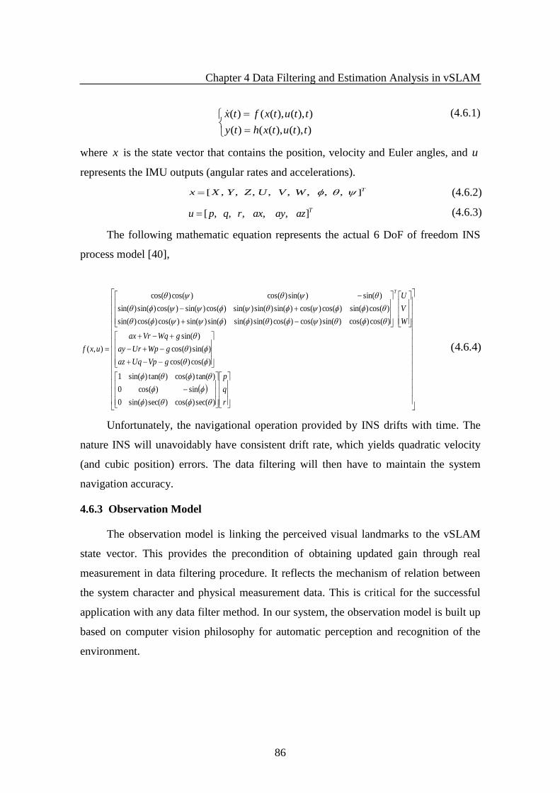
Chapter 4 Data Filtering and Estimation Analysis in vSLAM
86
)),(),(()(
)),(),(()(
ttutxhty
ttutxftx
(4.6.1)
where x is the state vector that contains the position, velocity and Euler angles, and u
represents the IMU outputs (angular rates and accelerations).
TWVUZYXx ],,,,,,,,[ (4.6.2)
Tazayaxrqpu ],,,,,[ (4.6.3)
The following mathematic equation represents the actual 6 DoF of freedom INS
process model [40],
r
q
p
gVpUqaz
gWpUray
gWqVrax
W
V
U
uxf
T
)sec()cos()sec()sin(0
sin)cos(0
)tan()cos()tan()sin(1
)cos()cos(
)sin()cos(
)sin(
)cos()cos()sin()cos()cos()sin()sin()sin()sin()cos()cos()sin(
)cos()sin()cos()cos()sin()sin()sin()cos()sin()cos()sin()sin(
)sin()sin()cos()cos()cos(
),(
Unfortunately, the navigational operation provided by INS drifts with time. The
nature INS will unavoidably have consistent drift rate, which yields quadratic velocity
(and cubic position) errors. The data filtering will then have to maintain the system
navigation accuracy.
4.6.3 Observation Model
The observation model is linking the perceived visual landmarks to the vSLAM
state vector. This provides the precondition of obtaining updated gain through real
measurement in data filtering procedure. It reflects the mechanism of relation between
the system character and physical measurement data. This is critical for the successful
application with any data filter method. In our system, the observation model is built up
based on computer vision philosophy for automatic perception and recognition of the
environment.
)4.6.4(

Chapter 4 Data Filtering and Estimation Analysis in vSLAM
87
4.6.3.1 3D Coordinates in Camera Model
As indicated in Chapter3, perspective camera model is formulated by intrinsic and
extrinsic parameters, which ensures the geometric transformation between
camera/image and world/camera reference frames respectively as shown in Figure
(4.6.1).
Figure 4.6.1 Camera model [40]
The intrinsic parameters of a camera can be simply consist of the horizontal and
vertical scale factor ( vk and uk ), the image centre coordinates ( 0u , 0v ) given in the
image frame and the focal distance f . Thus, the concise intrinsic parameters in a camera
matrix used in this research are defined as:
0
0
0 0
0 0
0 0 1 0
u
c v
u
I v
where u u
v v
f k
f k
Extrinsic parameters define the transformation relation from the world to camera
frame given by the homogeneity matrix A .
11 12 13
21 22 23
31 32 33 0 1
0 0 0 1
x
y
z
r r r t
r r r t R tA
r r r t
The matrix A is a combination of a rotation matrix R and a translation t from
the world frame to the camera frame. Obviously, the matrix A changes with the camera
(UAV) displacement.
On the precondition that the necessary parameters of camera are ready through
camera calibration methods [6, 24, 69, 90] in Chapter 3, the coordinates in
corresponding frames can be achieved by triangulation principle [61, 69] in epipolar
geometry as Figure 4.6.2.
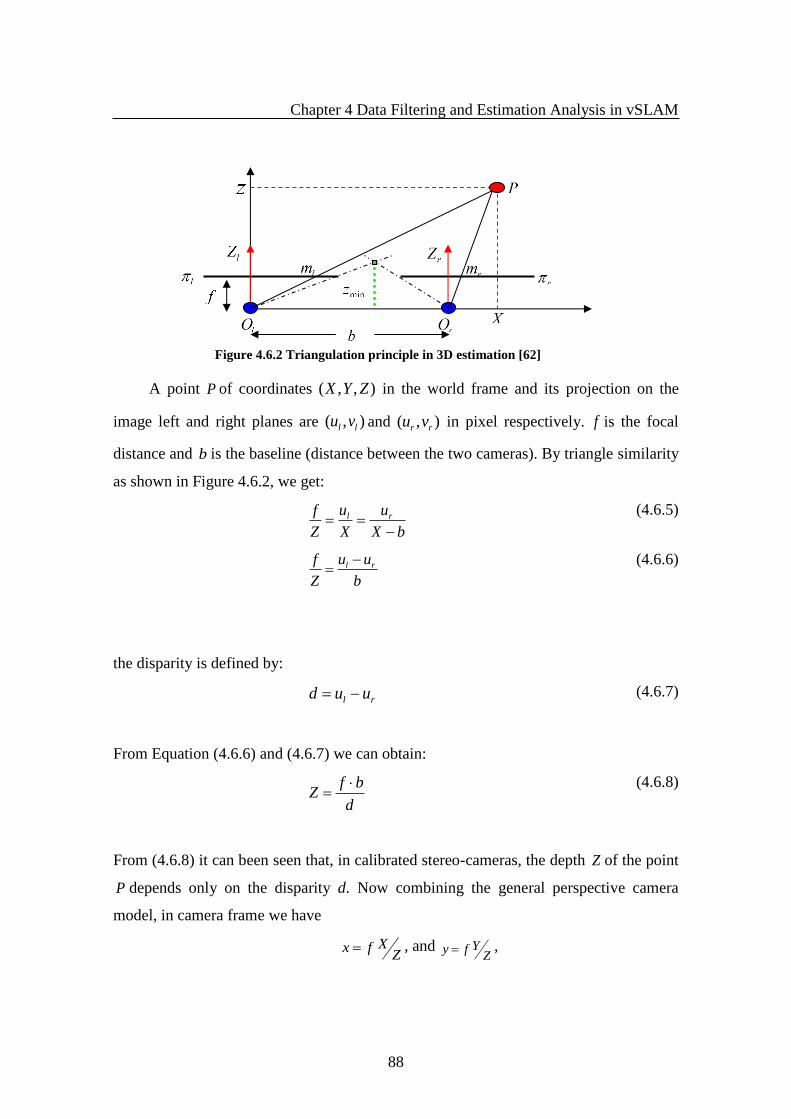
Chapter 4 Data Filtering and Estimation Analysis in vSLAM
88
A point P of coordinates ),,( ZYX in the world frame and its projection on the
image left and right planes are ),( ll vu and ),( rr vu in pixel respectively. f is the focal
distance and b is the baseline (distance between the two cameras). By triangle similarity
as shown in Figure 4.6.2, we get:
bX
u
X
u
Z
f rl
(4.6.5)
b
uu
Z
f rl (4.6.6)
the disparity is defined by:
rl uud (4.6.7)
From Equation (4.6.6) and (4.6.7) we can obtain:
d
bfZ
(4.6.8)
From (4.6.8) it can been seen that, in calibrated stereo-cameras, the depth Z of the point
P depends only on the disparity d. Now combining the general perspective camera
model, in camera frame we have
ZXfx , and
ZYfy ,
Figure 4.6.2 Triangulation principle in 3D estimation [62]

Chapter 4 Data Filtering and Estimation Analysis in vSLAM
89
which can be translated to retinal plane with pixel coordinates in the perspective camera
as shown in Figure 4.6.3 to have
(4.6.9)
where, the focal length is f, pixel size is sx and sy in two dimensions, the image centre ox
and oy , ),( imim yx is image coordinates in pixels.
The relation presented above depicts that two images from one 3D point are
needed to determine the 3D coordinates in Euclidean space. Given those two images
obtained by two cameras, both the intrinsic and extrinsic parameters as Tand,,,
need to be available in one consistent reference frame.
Below, we summarise the procedure for calculation of the 3D coordinates and
image coordinates [61, 69].
Step 1: Transform into camera coordinates
(4.6.10)
Step 2: Transform into image coordinates in pixels
x
x
im oZ
X
s
fx
y
y
im oZ
Y
s
fy
f Z
Z
Xfx
X
O
x
Figure 4.6.3 Perspective camera model
Z
Y
X
W
W
W
C
C
C
T
T
T
Z
Y
X
Z
Y
X
cossin0
sincos0
001
cos0sin
010
sin0cos
100
0cossin
0sincos
~
~
~
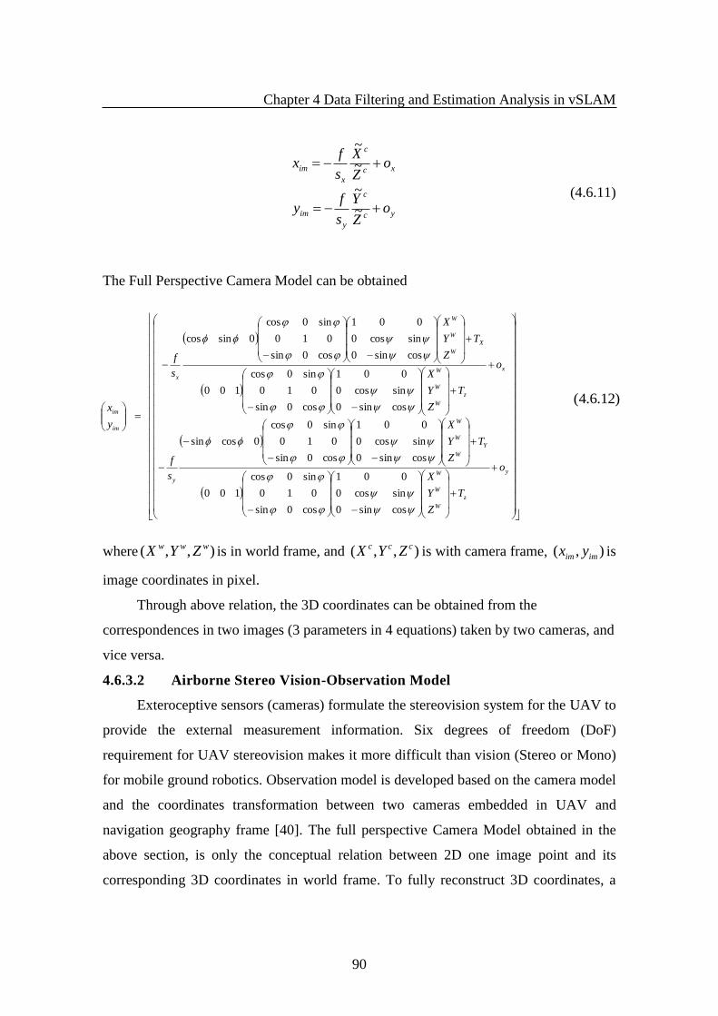
Chapter 4 Data Filtering and Estimation Analysis in vSLAM
90
(4.6.11)
The Full Perspective Camera Model can be obtained
where ),,( www ZYX is in world frame, and ),,( ccc ZYX is with camera frame, ),( imim yx is
image coordinates in pixel.
Through above relation, the 3D coordinates can be obtained from the
correspondences in two images (3 parameters in 4 equations) taken by two cameras, and
vice versa.
4.6.3.2 Airborne Stereo Vision-Observation Model
Exteroceptive sensors (cameras) formulate the stereovision system for the UAV to
provide the external measurement information. Six degrees of freedom (DoF)
requirement for UAV stereovision makes it more difficult than vision (Stereo or Mono)
for mobile ground robotics. Observation model is developed based on the camera model
and the coordinates transformation between two cameras embedded in UAV and
navigation geography frame [40]. The full perspective Camera Model obtained in the
above section, is only the conceptual relation between 2D one image point and its
corresponding 3D coordinates in world frame. To fully reconstruct 3D coordinates, a
yc
c
y
im
xc
c
x
im
oZ
Y
s
fy
oZ
X
s
fx
~
~
~
~
y
z
W
W
W
Y
W
W
W
y
x
z
W
W
W
X
W
W
W
x
im
im
o
T
Z
Y
X
T
Z
Y
X
s
f
o
T
Z
Y
X
T
Z
Y
X
s
f
y
x
cossin0
sincos0
001
cos0sin
010
sin0cos
100
cossin0
sincos0
001
cos0sin
010
sin0cos
0cossin
cossin0
sincos0
001
cos0sin
010
sin0cos
100
cossin0
sincos0
001
cos0sin
010
sin0cos
0sincos
)12.6.4(

Chapter 4 Data Filtering and Estimation Analysis in vSLAM
91
pair of image features are required based on feature matching methods in Chapter 3.
Therefore, the observation model, linking the perceived visual landmarks to the vSLAM
states vector is given by [40]:
1 1 1 1
11 12 13 141 1 1 1 1
31 32 33 34
1 1 1 1
21 22 23 241 1 1 1 1
31 32 33 34
2 2 2 2
11 12 13 142 2 2
31 32
c n c n c n c
mi mi mi
c n c n c n c
mi mi mi
c n c n c n c
mi mi mi
c n c n c n c
mi mi mi
c n c n c n c
mi mi mi
c n c
mi
m x m y m z mu
m x m y m z m
m x m y m z mv
m x m y m z m
m x m y m z mu
m x m y
2 2
33 34
2 2 2 2
21 22 23 242 2 2 2 2
31 32 33 34
n c n c
mi mi
c n c n c n c
mi mi mi
c n c n c n c
mi mi mi
m z m
m x m y m z mv
m x m y m z m
(4.6.13)
where [ ]n n n T
mi mi mix y z is the coordinate of the landmark im in the navigation frame
(NED). 1c
ijm and 2c
ijm are the components of 1
1 1( )n
c cI Mh and 1
2 2( )n
c cI Mh , which are
defined by camera intrinsic and extrinsic parameters respectively. This model can
provide the relation of image coordinates to coordinates in navigation frame and vice
versa with its inverse form.
In fully connected C-vSLAM, those system models residing on individual nodes
are the same, the estimates obtained by each node are exactly the same for all nodes. By
information filter (EIF), each node receives all information contribution from the other
nodes, the global estimates obtained locally by EIF are all the same as centralised C-
vSLAM under full rate communication available [7].
4.6.3.3 The State Structure of UAV vSLAM
The state vector in UAV vSLAM in this research is given in as [ ]v mx x x , where
[ , , , , , , , , ]T
x X Y Z U V Wv and
1 2 3[ ... ]m Nx m m m m with xv is the
state vector of the UAV; mx is the state vector of the landmark observed. The estimated
error covariance kkP / for the system can be written as:

Chapter 4 Data Filtering and Estimation Analysis in vSLAM
92
1
1 11 1
/
1
( / ) ( / ) ... ( / )
( / ) ( / ) ... ( / )
( / ) ( / ) ... ( / )
vv v vN
v N
k k
Nv N NN
P k k P k k P k k
P k k P k k P k kP
P k k P k k P k k
(4.6.14)
The sub-matrices ( / )vvP k k , ( / )viP k k , ( / )iiP k k Ni ,...1 , sampling at time k , are the
vehicle-to-vehicle, vehicle-to-landmark and landmark-to-landmark covariances.
4.7 Experimental Study
In this section, experiment tests were carried out for the estimation of position and
attitudes of a UAV through vSLAM with both process and binocular observation
models detailed in the previous section. This implemented aerial vSLAM has an
iterative procedure as shown in Figure 2.4.1.
4.7.1 Experiment Setup
The tests were performed on the segmented data set taken by Colibri III mini
UAV (Figure 4.7.1) during flight trials conducted at UPM (Universidad Polit´ecnica de
Madrid).
Figure 4.7.1 UAV used in the tests [153]
The testbed Colibri III [153] is fitted with internal sensors (GPS, IMU) and a
firewire color camera for acquiring the images.
The settings in the feature extraction algorithms of SIFT/SURF were default as in
[12, 17]. The relative estimation error rates (RERs) were calculated by a set of runs (‘R-
’ in table) for the quantitative analysis to determine the relative performance of the
filtering algorithms described in the preceding sections.
The test was conducted over a 100 time steps per run, with a sequence of 100
calibrated stereo aerial images captured synchronously in the air during an actual flight.

Chapter 4 Data Filtering and Estimation Analysis in vSLAM
93
The real flight trajectory was recorded from a GPS derived navigation solution. GPS
measurement was used as a ground truth, which is actually a differential GPS (it is
default in this thesis).
The noise was applied on the input control vector for the flight's rotation and
acceleration rates as . The corresponding noise scale was ranged
in vector 1w = [pi/180, pi/180, pi/180, 1.8, 1.8, 1.8]T which was referenced from the real
system. 2w is twice of 1w . 3w =2*[pi/180, pi/180, pi/180, 2.8, 2.8, 2.8] with 4w is
twice of 3w . Each scale was repeatedly used by 10 runs with different noise utilised by a
random coefficient for each run. The same noise setting was consistent cross the
different algorithms to facilitate direct comparison and statistics against their
performance.
The observation noise was applied by a value of 10 on the diagonal element of the
covariance of a 4×4 matrix derived from the stereo camera model.
The relative error rates (RERs) were calculated as following:
Firstly, the SLAM/INS error rate was noted for each run respectively. Then those
error rates were summed against the ground truth in the whole (10 runs) along 3
dimensional axis separately. The results were then divided by the total number of time
steps (100) to get the average error rate along each dimension. Finally, the relative error
rate was calculated using the average error rate of (x,y,z) in SLAM and dividing it by
the average INS error. After this, the error rate for all dimensions was divided by the
total number of dimensions (three in this case). The smallest ratio is corresponded to the
best estimate.
4.7.2 Filters Test with SIFT
In this test, estimation algorithms (EKF, EIF, UKF and UHF) were combined with
the SIFT feature extraction method and tested against a sequence of noise scales with
results in Table 4.7.1.
The relative error rate obtained in Table 4.7.1 shows that EIF and EKF were more
impressive than the other two filters (UKF, UHF) in this experiment. This was assessed
against each run’s criteria and average error result (denoted as initial ‘ave’ in the table).
Overall the best filtering results were obtained by EIF.
Tazayaxrqpu ],,,,,[

Chapter 4 Data Filtering and Estimation Analysis in vSLAM
94
UHF slightly outperformed UKF which had the highest error rates. This is
consistent with the analysis in the theory section. Both UKF and UHF did not obtain the
convincing results expected, although this can be somehow compensated by the merits
of UHF that has no constraint with noise assumption.
When the noise scale was increased, it was interesting to note that the relative
error rates did not go up accordingly. Instead, in most of cases, the RERs were seen to
decrease. This leads us to conclude that those filters have enhanced tolerance to noise.
Their relative performance was even improved instead of deteriorating.
In this evaluation, both EIF and EKF demonstrated quite similar robust
consistency characteristics, and proved to be more reliable and robust than UHF and
UKF.
Table 4.7.1 RERs (SLAM-INS) of Filters with SIFT applied
Noise scale/test
Algorithm/
Run
w1-test1 w2-test2 w3-test3 w4-test4
EIF R1 .068 .049 .045 .028
R2 .091 .058 .049 .055
R3 .223 .150 .055 .058
Ave .127 .086 .050 .047
EKF R1 .113 .055 .055 .088
R2 .160 .088 .095 .088
R3 .419 .151 .148 .101
Ave .231 .098 .099 .092
UHF R1 .257 .140 .109 .161
R2 .317 .237 .124 .162
R3 .615 .283 .124 .221
Ave .396 .220 .119 .182
UKF R1 .177 .150 .176 .134
R2 .267 .281 .191 .317
R3 .734 .299 .205 .442
Ave .392 .243 .191 .298
4.7.3 Filters test with SURF
In this evaluation, the SURF method was used and the relative error rates obtained
are in Table 4.7.2.

Chapter 4 Data Filtering and Estimation Analysis in vSLAM
95
Table 4.7.2 RERs (SLAM-INS) of Filters with SURF applied
Noise scale/test
Algorithm/
Run
w1-test1 w2-test2 w3-test3 w4 -test4
EIF R1 .139 .138 .132 .278
R2 .177 .139 .175 .297
R3 .181 .178 .192 .368
Ave .166 .152 .166 .308
EKF R1 .091 .091 .097 .239
R2 .093 .121 .100 .427
R3 .299 .174 .550 .849
Ave .161 .129 .249 .505
UHF R1 .144 .163 .158 .162
R2 .345 .215 .173 .216
R3 .378 .300 .181 .251
Ave .289 .226 .171 .210
UKF R1 .383 .146 .141 .134
R2 .479 .186 .199 .317
R3 .589 .195 .207 .442
Ave .484 .175 .182 .298
The test data obtained in Table 4.7.2 showed that, when SURF method is utilised
for feature extraction and matching, the overall performance of EIF and EKF are very
similar. EKF is slightly better than EIF under the lower noise scale condition of test1
and test 2, while EIF outperformed EKF when noise scale was increased as in last two
tests.
When compared with UKF, UHF demonstrated better performance although both
techniques are ranked below EIF/EKF. However, under certain conditions, such as test
2 (Table 4.7.2), UKF slightly out performs UHF, but on average, UHF performances
overtook UKF. This is the same impression as when the comparison was conducted
with SIFT.
To comprehensively conclude all the evaluations above, the overall estimation
accuracy of all filters is slightly inferior when SURF is utilised. This implies that the
SIFT is the more advantageous than SURF in this specific stereo vision scenario based
aerial vSLAM.

Chapter 4 Data Filtering and Estimation Analysis in vSLAM
96
4.8 Summary and Discussion
The successful utilisation of various filter algorithms with SIFT/SURF feature
extraction techniques in this visual SLAM scheme opened the door for evaluation of
their feasibility and effectiveness in terms of relative error rates.
The overall results were encouraging, especially for the EIF and EKF in this
vSLAM application, implying their performance was consistent with that predicted in
the literature [37, 38]. In most cases, EIF demonstrated the overwhelming performance
advantage over the other filters. This result points to the potential suitability for the use
of EIF in C-vSLAM in preference to the other filter implementation methods. It was
noted a slight performance difference when utilising SIFT over SURF for feature
matching.
The evaluation results presented for UKF seem inconsistent with the literatures [4,
33]. As theoretically, UKF should perform better against nonlinear environments. In our
case, UKF did not behave ideally as expected. After examining the study, we have the
following conclusions:
During the UKF test, we found that the error covariance was always ill-
conditioned and non-negative definiteness was not guaranteed even with “diagonal
loading” [42] used as the treatment for singularity. Covariance was still not invertible,
due to the negative definiteness. Therefore, Cholesky decomposition could not be
fulfilled as the theory demands, and the alternative methods, such as SVD
decomposition were utilised. High singularity of error covariance and negative
definiteness frequently occurred during the filtering procedure. We believe this was
caused by the inherent high non-linearity of our system.
The same was found to occur for UHF processing, although it did produce better
results than UKF, because of its fundamental merits [4] that can only make up to certain
extent for the effects derived from an ill-conditioned error covariance matrix. However,
the overall errors cannot be dismissed simply by its merits above.
Against these criteria, UKF/UHF are both the least suitable candidates for the
proposed UAV vSLAM application. Ongoing efforts need to be given on producing the
optimal UKF/UHF combination, to improve their combined filtering performance,
through elimination of any ill-conditioned covariance matrices.

Chapter 4 Data Filtering and Estimation Analysis in vSLAM
97
As feature extraction methods, both SIFT and SURF performed reasonably well.
The overall slightly superior performance of SIFT may have resulted from the effects of
the differing matched feature pairs extracted by the respective algorithm. Apart from the
inherent advantage of 128- element SIFT descriptor. They also rely on parameters such
as matching thresholds which need to be tuned to meet the various application
environments. SURF was undoubtedly proved the faster method. The further tuning of
all such parameters is crucial for their successful application with the different filter
combinations and corresponding feature extraction and matching method. All such
parameters had a large effect on the filters’ performance. As such, the need to ascertain
and maintain a certain number of appropriate landmarks in the state vector is necessary
for EIF/EKF. Both of them demonstrate deteriorated performance while small
covariance matrix turned up under low number of available features.
The actual running time did not form part of the analysis in those programming
codes. However, EIF/EKF was both similar in run time and faster than the equivalent
pair of UKF/UHF which ran in similar execution periods.
From the experimental evaluation results presented, we can conclude that the
proposed algorithms EIF/EKF are valid for handling real data sets in aerial vSLAM.
Whilst the current results appear promising, there are still certain limitations of the
proposed filtering method due to factors such as the inherent limited robustness of both
the filters and the performance/suitability of the feature extraction algorithms under the
stress of uncertainty, as found in real world environments. Thus, it is evident that there
are still challenges to overcome.

Chapter 5 3D Reconstruction with Textured Mapping in Aerial vSLAM
98
CHAPTER 5
3D Reconstruction with Textured Mapping in Aerial vSLAM
In this chapter, the goal is to recover a meshed model from a multi-view image
sequence taken by onboard stereo cameras from an air vehicle, and to perform a surface
reconstruction based on the 3D points obtained within SLAM procedure. We aim to
combine various techniques and propose effective methods to provide a panorama style
textured mapping to handle large-scale scenes. This not only provides viewers with
well visualised view, but also provides enriched environmental information for visual
navigation.
5.1 Introduction
3D reconstruction, aiming to develop a three-dimensional model of an object from
several two-dimensional views, can be defined as the process of capturing the shape and
appearance of real objects. It has long attracted the efforts of researchers from areas of
computer vision and photogrammetry, and found various applications in surface
reconstruction based on 3D point clouds drawn from the fields of computer vision,
graphics and computational geometry. This application has been traditionally focusing
on virtual reality or the preservation of historical heritage type of application.
Most of the data acquisition in early works was through laser devices whose
probing points are dense and well distributed [82]. Although these reconstructions have
been reported as successful, they have normally targeted urban environments or
archaeological sites. The limitation of cost and weight makes laser scanners unable to be
loaded on all platforms. Furthermore, the outdoor environmental constraints make its
application non-universal under various situations.
Multi-view stereovision with digital cameras is a valuable alternative for outdoor
scene reconstruction. However, the challenges are still there. Features are likely to be
entangled with errors, redundancies, excessive outliers and noise, due to the image
quality and the process of the feature extraction and matching. This is especially true
when the 2D images are obtained from airborne vehicles. The vibration of the vehicles

Chapter 5 3D Reconstruction with Textured Mapping in Aerial vSLAM
99
can unexpectedly cause deterioration of the quality of images snapped in the air and
thus can degrade the final 3D presentation. Even more challenges are to be expected
when textured 3D mapping is performed using aerial images. Air vehicles present
challenges related to the 6DoF (Euclidian position and yaw, pitch, roll angles) motion
involved in its dynamics. This has largely increased the nonlinearity of system
modelling, which lowers the expected robustness. General reconstruction methods
cannot therefore be simply transferred to terrain environments within an air vehicle
based application.
Nowadays, impressive progress has been made in 3D reconstruction in the
computer vision community as well as vSLAM (Simultaneous Localisation and
Mapping) in the robotics community [57]. In visual SLAM, tracking and reconstruction
have a high inter-dependency [58], i.e., a good 3D reconstruction of the environment is
necessary for correct tracking, and good tracking is required for a correct reconstruction
of the environment. Therefore, a good integration of 3D reconstruction from computer
vision with vSLAM can deliver effective visualisation of large scale models based on
onboard vision systems and can improve the accuracy of depth estimation by optimised
triangulation angles. It can also increase the reliability for localisation.
We thus introduce textured 3D mapping of the scene for an air vehicle-based
vSLAM models in this research project. The obtained visualisations using such data are
possible in the form of panoramic mosaics [59, 60] or simple geometric models [61].
Texture mapping with 3D reconstruction in vSLAM, is the process of integrating
the information (spatial and shade) obtained by visual sensors (cameras) into a
consistent model and describing that information as a given representation. The
estimated 3D poses of landmarks are obtained by the vSLAM algorithm [12] with an
observation model [5] based on the principle of 3D reconstruction in epipolar geometry
[13]. The 3D reconstruction in this case is, then, under interaction between vSLAM and
epipolar geometry [13], where the camera viewpoints are provided by data fusing
methods used in vSLAM embedded on air vehicles. With a space transformation in
corresponding reference frames (image → air vehicle → world frame) and mapping

Chapter 5 3D Reconstruction with Textured Mapping in Aerial vSLAM
100
algorithms employed in the stereo camera model [13], both landmarks and an air vehicle
3D coordinates can be reconstructed.
In this research, we give insights into the landmark-based map that represents the
world as a set of spatially located features. One thing to be noted is that, due to the
limitation on power, memory and computation cost, the number of correspondences
used within vSLAM (especially on air vehicle) cannot be enough dense to form rich
texture for visualisation. Therefore, in this research, one emphasis is on the
reconstruction of sparse distinct terrain features to present a wider view of the scene,
hence, covering more field information. Such representation is compact to meet the
need for operating in large environments [62].
The construction of a robust and reliable 3D map of the environment requires
invariant and distinctive features from the images. As a solution, both SIFT (Scale
Invariant Feature Transform)[12] and SURF (Speeded up robust features) [17]
algorithms, described in chapter 2, were adopted for comparison purposes.
With these extracted 2D correspondences and the triangulation principle,
calibrated stereo cameras with known internal (intrinsic) and external (extrinsic)
parameters of each camera are used to reconstruct 3D points from 2D calibrated images
synchronised with a set of tracks. With these known calibration parameters, the location
of a 2D marker image on a camera can be converted into a ray as shown in Figure3.2.1
in Chapter 3. The ray originates at the focal point of the camera (without errors
considered) and intersects the 3D position of the marker in space. By using two cameras,
we can therefore pinpoint the location of a marker through the inverse camera model
described in chapter 4.6. This is the principle of 3D reconstruction developed in
epipolar geometry [61] as in Figure 5.6.1. The position of cameras is obtained through
the estimation with vSLAM during data fusion processing, which has been specified in
chapter 3 and chapter 4.
5.2 3D Reconstruction Pipeline Process
In this section, we use references [62, 64, 65, 69].
3D reconstruction from images or photographs has undergone a revolution during
the last decades. Coupled with rapid developments in digital imaging technology, the
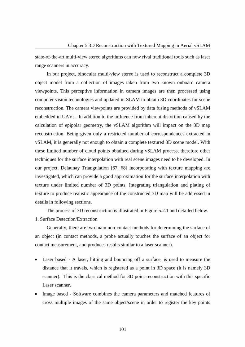
Chapter 5 3D Reconstruction with Textured Mapping in Aerial vSLAM
101
state-of-the-art multi-view stereo algorithms can now rival traditional tools such as laser
range scanners in accuracy.
In our project, binocular multi-view stereo is used to reconstruct a complete 3D
object model from a collection of images taken from two known onboard camera
viewpoints. This perceptive information in camera images are then processed using
computer vision technologies and updated in SLAM to obtain 3D coordinates for scene
reconstruction. The camera viewpoints are provided by data fusing methods of vSLAM
embedded in UAVs. In addition to the influence from inherent distortion caused by the
calculation of epipolar geometry, the vSLAM algorithm will impact on the 3D map
reconstruction. Being given only a restricted number of correspondences extracted in
vSLAM, it is generally not enough to obtain a complete textured 3D scene model. With
these limited number of cloud points obtained during vSLAM process, therefore other
techniques for the surface interpolation with real scene images need to be developed. In
our project, Delaunay Triangulation [67, 68] incorporating with texture mapping are
investigated, which can provide a good approximation for the surface interpolation with
texture under limited number of 3D points. Integrating triangulation and plating of
texture to produce realistic appearance of the constructed 3D map will be addressed in
details in following sections.
The process of 3D reconstruction is illustrated in Figure 5.2.1 and detailed below.
1. Surface Detection/Extraction
Generally, there are two main non-contact methods for determining the surface of
an object (in contact methods, a probe actually touches the surface of an object for
contact measurement, and produces results similar to a laser scanner).
Laser based - A laser, hitting and bouncing off a surface, is used to measure the
distance that it travels, which is registered as a point in 3D space (it is namely 3D
scanner). This is the classical method for 3D point reconstruction with this specific
Laser scanner.
Image based - Software combines the camera parameters and matched features of
cross multiple images of the same object/scene in order to register the key points

Chapter 5 3D Reconstruction with Textured Mapping in Aerial vSLAM
102
with the known cameras position and its relation to the object. This image based
method is adopted in our application.
2. Points cloud creation
A set of vertices in 3D space is created to form a dense cloud. The more points
that are available, the more vivid the picture is. This cloud includes the normals (the
direction that each point is “facing”) and/or colour data (RGB values) of each point.
3. Surface Reconstruction
Complex mathematics is used to connect the dots to create numerous polygons or
faces, namely a surface mesh or wire frame. This process may include mesh repair/hole
filling if the features are not close by in traditional surface building. This may not be
practical when dynamical construction is involved within real time vSLAM (In this
research, we developed a strategy to make up by adding extra non salient features).
4. Texture Mapping/Rendering
Texture mapping/Rendering or Plating is a method for adding surface texture
(images) or colour to each face on the surface mesh. This process includes UV (where
UV refers to pixel axes of the 2D texture) mapping which means to “unwrapping” the
surface mesh to create a 2D image file and mapping the surface texture to the UV file.
In our research, image based methods are engaged. Surface Detection/Extraction
based on related techniques are the first step in order to find correspondences in two
images. With those correspondences, the triangulation algorithm in epipolar geometry is
then applied to produce the 3D point cloud with space transformation in the
corresponding reference frames (image → UAV→ world frame, etc.). The limited
number of points then needs to be interpolated for the reconstruction of the surface. To
do so, the triangulation based 3D reconstructed vertices are used to create the faces of
Points Cloud
Creation
Surface
Reconstruction
Surface
Detection/Extraction
Texture
Mapping/Rendering
Figure 5.2.1 Process of 3D Reconstruction

Chapter 5 3D Reconstruction with Textured Mapping in Aerial vSLAM
103
the object. Texture mapping is then used to plate the triangulated surface with
corresponding real images in the 2D image plane for a realistic scene. This means filling
the triangulation surface in 3D space with their triangulated 2D image formed by the
same vertices via projection between 3D coordinates and 2D pixels using projection
transformation. The reconstructed faces are thereafter directly displayed in 3D points
overview or the rendered 3D coordinates window on the display screen.
5.3 Homogeneous Coordinates and Homography
Homogeneous coordinates [69,70] are a system of coordinates used in projective
geometry much as Cartesian coordinates are used in Euclidean geometry. This is the
basis of transformation between 3D space and 2D images. Their main advantage is that
the coordinates of points at infinity can be represented using finite coordinates.
Formulas involving homogeneous coordinates are often simpler and more symmetric
than their Cartesian counterparts. Homogeneous coordinates have found wide
applications in computer graphics and 3D computer vision, where both affine and
projective transformations can be easily represented by a matrix.
Homogeneous coordinates have a natural application to computer graphics, which
provide a basic formation for the extensively used projective geometry to project a
three-dimensional scene onto a two-dimensional image plane. With homogeneous
coordinates, if a point is multiplied by a non-zero scalar, the resulting coordinates still
represent the same point. With an additional condition added on the coordinates, it can
be ensured that only one set of coordinates corresponds to a given point. The number of
coordinates required is generally one more than the dimension of the projective space
being considered. One needs two homogeneous coordinates to specify a point on the
projective line, while three homogeneous coordinates are required to specify a point on
the projective plane.
To simplify the concept, a 2D point (x, y) in an image can be represented as a 3D
vector ''' ,z,yx where '/','/' zyyzxx . This is called the homogeneous
representation of the point and it lies on the projective plane 2P . The point (x, y)
corresponds to the triple ''' ,z,yx = ''' ,kz,kykx where z ≠ 0. Such a triple is a set of

Chapter 5 3D Reconstruction with Textured Mapping in Aerial vSLAM
104
homogeneous coordinates for the point (x, y). Homogeneous representation of lines can
be written as
It is the equivalence class of vectors, and any vector is a representative set of all
equivalence classes in R3(0,0,0)
T forms P
2.
Homogeneous representation of points:
x=(x,y)T on l=(a,b,c)
T if and only if ax+by+c=0
(x,y,1)(a,b,c)T=(x,y,1)l=0 (x,y,1)
T~ k(x,y,1)
T, k 0
Summary of homogenous representation:
A triple (X, Y, Z) is needed to represent a point in the projective plane, which is
the homogeneous coordinates of the point with at least one of X, Y and Z not 0.
Multiplied by a common scale/factor, homogeneous coordinates still represent
the same point.
The homogenous representation represents the point (X/Z, Y/Z) in the Euclidean
plane when Z ≠ 0.
The homogenous representation represents the point at infinity while Z = 0.
The omitted triple (0, 0, 0) does not represent any point. The origin is depicted at
instead.
A homography [23, 69] is an invertible mapping of points and lines on the
projective plane 2P . In homogeneous coordinate notation, the homography is a plane to
plane transformation represented by the formulas in projective space – 3x3 matrix H
such that vector HXX ' implements the corresponding points from 2D image
coordinate to 3D real world(see below).
Tcbacbyax ),,(0
0,0)()( kkcykbxka TTa,b,cka,b,c ~
Homogeneous representation of points
on if and only if

Chapter 5 3D Reconstruction with Textured Mapping in Aerial vSLAM
105
The matrix H can be changed by multiplying an arbitrary non-zero constant
without altering the projective transformation. Thus, H is considered as a homogeneous
matrix with only 8 degrees of freedom even though it contains 9 elements. This means
there are 8 unknowns that need to be solved for. Therefore, converting a homogenous
point (x,y,1) (camera reference frame) to image coordinate (u,v,1) (image reference
frame) can be implemented by the homogenous matrix H.
There are a few different methods to obtain H, and the Direct Linear Transform
(DLT) algorithm is the classical algorithm used to solve for the homography matrix H
given a sufficient set of point correspondences. 4 pairs of 2-D points are sufficient to
determine it. Details can be found in [23, 69, 70].
5.4 3D Textured Mapping
In practice, the 3D model built up based on the principles in the above section can
only generate a certain number of sparse cloud points, and may not be able to present a
good visualisation of the actual object in the stereo image pair. Those cloud points are
normally only able to verify whether the 3D coordinates needed for the reconstruction
were successful, and are not enough to show the real scene. For the sake of visualisation,
the limited number of 3D points obtained from the above algorithm then need to be
interpolated to produce triangulated surface that can further be plated with images taken
by camera. Each point is reconstructed and assigned with the pixel value from image
textures. With the interpolation technique, we can achieve more accurate and vivid
results.
5.4.1 3D Surface Meshing
The construction of a 3D map is based on meshing and texture wrapping. Two
ways are usually used to achieve this [71, 72]. One is based on the wrap of the 2D
image texture onto a 3D mesh. This requires a dense representation of the scene.
11
y
x
Hv
u
333232
232222
131211
,
hhh
hhh
hhh
Hand

Chapter 5 3D Reconstruction with Textured Mapping in Aerial vSLAM
106
Otherwise, the texture will not be well aligned on the geometric form of the scene. The
other method is based on the triangulation of the 3D feature points (extracted by
SIFT/SURF and optimised with vSLAM in our project). Through the projection of the
corresponding image to texture each triangle, this method performs better in terms of
visualisation and is more accurate when building a texture map. The plating (or
mapping) of colour (or texture) consists of covering the surfaces of an object by the
corresponding images. The plating of textures is largely used in image synthesis in
order to improve the quality of the constructed map. It requires a grid that is a
geometrical arrangement of the pixels in the image, which consists of different types of
geometrical shapes, such as square, hexagonal, or triangular. In our research, the
triangulation (grid) of “Delaunay” [73] is incorporated due to its advantage on
contiguous non-overlapping triangles, which are as equi-angular as possible. Thus, it
can reduce potential numerical precision problems created by long skinny triangles. It is
independence of the order the points processed, which also ensures that any point on the
surface is as close as possible to a node. Benefitting from those advantages, we can then
approximate the peaks and valleys of a surface with a limited number of sample points
efficiently and produce something that appears natural.
The principle of Delaunay Triangulation (DT) for N points is that the single
triangulation with corresponding circumcircle passing by the three points of a triangle
does not contain any other point (see Figure 5.4.1). The DT is the best in terms of
maximising the smallest internal angles shown in Figure 5.4.2 to form a "mesh" as
depicted in RHS of Figure 5.4.1.
DT is the dual of the Voronoï diagram (Figure 5.4.3 in black solid) that is
formulated by the linking of the circumcircle centrals of the Delaunay Triangulation.
The Voronoï diagram is generated from a set of points E, called sites or germs, in
the same plan. Each point of E is inside a convex polygon (Figure 5.4.3). This latter
delimits a surface constructed by points of the plan, which are closer to this site than
other sites. Each obtained a polygon is called polygon of Voronoï [74, 75]. The nodes of
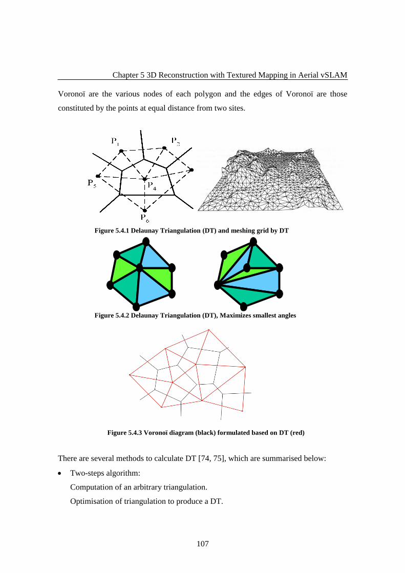
Chapter 5 3D Reconstruction with Textured Mapping in Aerial vSLAM
107
Voronoï are the various nodes of each polygon and the edges of Voronoï are those
constituted by the points at equal distance from two sites.
There are several methods to calculate DT [74, 75], which are summarised below:
Two-steps algorithm:
Computation of an arbitrary triangulation.
Optimisation of triangulation to produce a DT.
Figure 5.4.1 Delaunay Triangulation (DT) and meshing grid by DT
Figure 5.4.3 Voronoï diagram (black) formulated based on DT (red)
Figure 5.4.2 Delaunay Triangulation (DT), Maximizes smallest angles
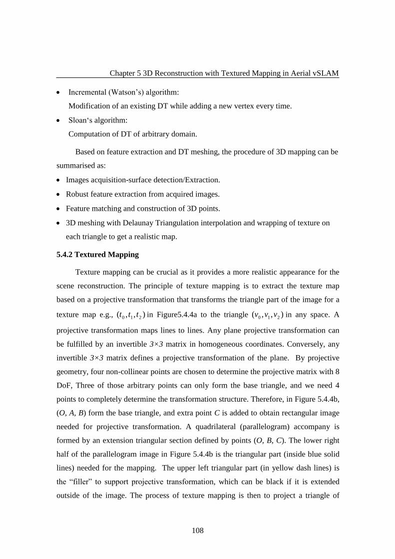
Chapter 5 3D Reconstruction with Textured Mapping in Aerial vSLAM
108
Incremental (Watson’s) algorithm:
Modification of an existing DT while adding a new vertex every time.
Sloan‘s algorithm:
Computation of DT of arbitrary domain.
Based on feature extraction and DT meshing, the procedure of 3D mapping can be
summarised as:
Images acquisition-surface detection/Extraction.
Robust feature extraction from acquired images.
Feature matching and construction of 3D points.
3D meshing with Delaunay Triangulation interpolation and wrapping of texture on
each triangle to get a realistic map.
5.4.2 Textured Mapping
Texture mapping can be crucial as it provides a more realistic appearance for the
scene reconstruction. The principle of texture mapping is to extract the texture map
based on a projective transformation that transforms the triangle part of the image for a
texture map e.g., ),,( 210 ttt in Figure5.4.4a to the triangle ),,( 210 vvv in any space. A
projective transformation maps lines to lines. Any plane projective transformation can
be fulfilled by an invertible 3×3 matrix in homogeneous coordinates. Conversely, any
invertible 3×3 matrix defines a projective transformation of the plane. By projective
geometry, four non-collinear points are chosen to determine the projective matrix with 8
DoF, Three of those arbitrary points can only form the base triangle, and we need 4
points to completely determine the transformation structure. Therefore, in Figure 5.4.4b,
(O, A, B) form the base triangle, and extra point C is added to obtain rectangular image
needed for projective transformation. A quadrilateral (parallelogram) accompany is
formed by an extension triangular section defined by points (O, B, C). The lower right
half of the parallelogram image in Figure 5.4.4b is the triangular part (inside blue solid
lines) needed for the mapping. The upper left triangular part (in yellow dash lines) is
the “filler” to support projective transformation, which can be black if it is extended
outside of the image. The process of texture mapping is then to project a triangle of
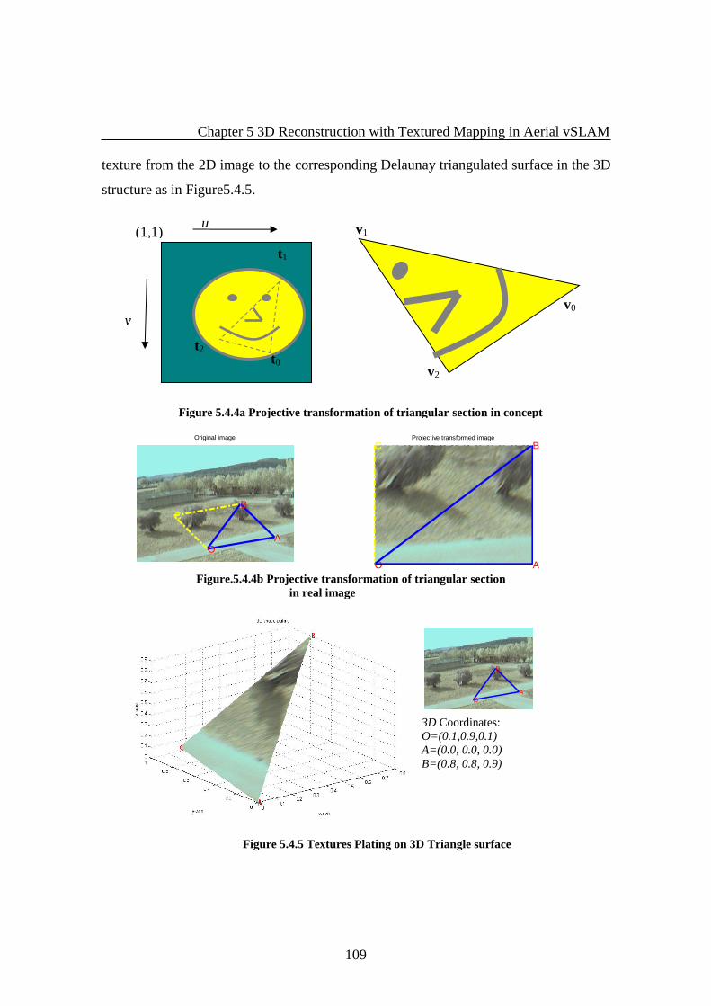
Chapter 5 3D Reconstruction with Textured Mapping in Aerial vSLAM
109
texture from the 2D image to the corresponding Delaunay triangulated surface in the 3D
structure as in Figure5.4.5.
Figure.5.4.4b Projective transformation of triangular section
in real image
3D Coordinates:
O=(0.1,0.9,0.1)
A=(0.0, 0.0, 0.0)
B=(0.8, 0.8, 0.9)
Figure 5.4.5 Textures Plating on 3D Triangle surface
Original image
OA
BC
Projective transformed image
O A
BC
OA
B
t2
t0
t1
(1,1) u
v
v0
v1
v2
Figure 5.4.4a Projective transformation of triangular section in concept

Chapter 5 3D Reconstruction with Textured Mapping in Aerial vSLAM
110
In detail rendering a texture mapped triangle is to assign the texture coordinates
(tx, ty) to the vertices. Then the tx and ty texture coordinates are interpolated across the
triangle, where a matrix transformation is used to transform the vertices from 2D image
space to 3D object space, and vice versa.
To use the above technique in a real application, we first select a piece (“cut off”)
from a reference image in the sequence of images as a texture, which is the lower right
triangle part in Figure.5.4.4b. Each triangular surface of the object is then covered with
a corresponding triangular image by interpolation. Since the position of the camera and
the position of the image of the object in 3D space are known, using the principle in
Figure 5.4.4, the result in Figure5.4.5 can be obtained consequentially.
The texture colour is usually blended with the interpolated RGB colour to
generate the final pixel colour. During this procedure, a sample texture is used to
determine the colour at each pixel in the image, and the elliptically shaped convolution
filters can be used for dealing with the aliasing problem [68, 69].
The effectiveness of the proposed techniques for textured 3D mapping with
verified later in section 5.6, where textured meshing is utilised with 3D construction
using real scene incorporating vSLAM.
5.5 Image Mosaicing
Image mosaicing has been an active research area in computer vision for many
years. Originally, the term image (photo) mosaic referred to compound images created
by stitching together a series of adjacent pictures of a scene. It is generally a process of
transforming different sets of data into one coordinate system – an image registration
which visually overlays two or more images of the same scene taken at different times
and different viewpoints, and/or by different sensors. Image mosaicing is a less
hardware-intensive technique to construct full view panoramas by aligning and pasting
images to cover a wider field of view image with "zipped" features that across over the
images [62]. Therefore, large scene images can be composited in a single form or
panorama when the cameras do not have wide fields of view, in order to capture large
real world scenes in one picture.

Chapter 5 3D Reconstruction with Textured Mapping in Aerial vSLAM
111
There have been a few recognized methods for image mosaicing, which can be
classified into two categories [Mallick, 83]:
Direct methods [142, 143], these are more applicable for mosaicing large
overlapping regions with small translations and rotations;
Feature based methods [69, 144, 145], these can usually tackle images with less
overlapped region and in general tend to be a bit more accurate but at the price
of intensive computation.
5.5.1 Technique Overview
In this research, a feature based image mosaicing technique for the UAV
environment will be constructed. Combining 3D mapping with images in different
frames is one of the applications of image mosaicing technique. The images acquired on
the UAV vary under both geometric and photometric changes, as 6 the DoF of UAV
leads to different geometrical transformations between the current and next image
frame. There may be also changes of the luminosity and contrast of the images with
UAV navigation in varying environments. To deal with these problems, we hence
conducted an investigation into the mosaic algorithm based on robust features
SIFT/SURF [12, 17], aiming to obtain a whole scene of the environment from the image
sequence, to generate a panorama for texturing the 3D scenario of the UAV trajectory.
The main challenges of image mosaicing can be summarised as follows:
Correction of geometric deformations using image data and/or camera models.
Image registration by image data and/or camera models.
Elimination of seams from image mosaics.
As introduced above, the main technique of image registration in image
mosaicking [62, 76, 79] is to match two or more images, i.e., project different images
to same reference (image) creating ‘one’ scene. This generally includes geometric
registration and photometric registration:
Geometric registration is the projective correspondence into one geographic
reference (common plane) to form a mosaic –by homography, FFT, correlation,
wavelet, etc.

Chapter 5 3D Reconstruction with Textured Mapping in Aerial vSLAM
112
Photometric registration is the projective correspondence into the same illumination
scale by linear regression.
The overall procedure of conducting mosaic imaging in our research can be
described as follows:
Take a sequence of overlapping images of a scene.
Compute the global transformation between the sensed image and the chosen
reference.
Transform the current image to overlap with the previous.
Blend the two images together at each step to create a mosaic.
Repeat if there are more images.
Here, the transformations of images can be classified as corresponding geometric
and photometric transformations with elements described as [62, 76, 79]:
• Geometric transformations
– Rotation
– Similarity (translation + uniform scale)
– Affine (scale dependent on direction)
• Photometric transformations
– Luminosity
– Contrast
– Affine intensity change.
5.5.2 Homography Transformation in Image Registration
In the context of this section, to register images geometrically refers to the process
of obtaining a dense correspondence (or registration) between multiple views of a planar
surface, where one of the images is referred to as the reference or source and the other
image is referred to as the target or sensed. In this case, the geometric transformation
between any two such views is obtained with an 8 DoF planar projective transformation
or homography [23, 24].

Chapter 5 3D Reconstruction with Textured Mapping in Aerial vSLAM
113
The homography transformation between two images is a linear transformation,
which only holds exactly when the imaged scene is planar or almost planar. This applies
to the situation of UAV at high altitude.
The homography that relates two given images is computed from sets of matches
between point features given by a feature tracker [62, 80, 81]. First we need to find all
matching (i.e., overlapping) images. Connected sets of image matches will later become
panoramas via mosaicing. RANSAC is applied to select a set of inliers that are
compatible with a homography between the images. The homography transformation
can then be obtained thereafter as well.
Depending on the frame-rate and the vehicle motion, the overlap between images
in the sequence is sometimes small. This generates a non-uniform distribution of the
features in the images [62, 76, 79, 80]. Hence, there may exist multiple solutions for the
homography matrix H.
In this research, feature based registration methods are adopted, which generally
have advantages over their direct correlation counterparts in terms of computation
speed, and the scope that they offer for the application of robust statistical methods for
outlier rejection [23]. As the planar homography has 8 DoF, each point correspondence
generates 2 linear equations for the elements of H and 4 correspondences are enough to
estimate the homography directly. If more than 4 points are available, a least-squares
solution can be found by linear methods. From the definition of H, we have
11
'
'
333231
232221
131211
y
x
hhh
hhh
hhh
y
x
(5.5.2)
where the equal sign “=” is equality up to scale. Each inhomogeneous 2D point
correspondence generates two linear equations in the elements of H.
0)('
0)('
232221333231
131211333231
hyhxhhyhxhy
hyhxhhyhxhx (5.5.3)
Hence, N points generate 2N linear equations, which may be arranged in a “design
matrix” [62] as:
AH=0

Chapter 5 3D Reconstruction with Textured Mapping in Aerial vSLAM
114
The solution for H is the one-dimensional kernel of A and is obtained from the SVD.
Under the condition that more than 4 points are obtained, a solution may be obtained by
minimising the algebraic residuals, r=AH, in the least-squares sense, then taking the
singular vector corresponding to the smallest singular value [84].
5.5.3 Mosaicing Compositing
In this section, we use references [79-81].
When applied within vSLAM, the first step in the image mosaicing technique is to
extract and match features between the consecutive onboard images based on
SIFT/SURF [12, 17] methods. The feature performances allow robust image
registrations that are necessary to compare or integrate the images obtained by cameras
in different time, position, etc.
The main problem in image compositing is the problem of determining how the
pixels in an overlapping area should be represented. The proposed mosaicing algorithm
is based on the SIFT/SURF detector/descriptor [12, 17, 76] for a robust matching
followed by estimating the homography for geometric registration. Figure 5.5.1 gives
the general steps of the mosaicing based homography approach incorporating with
SIFT/SURF detector/descriptor.
Image acquisition on UAV
Feature extraction
from image sequences
Homograhy H Estimation
Mosaicing images
Project the images
referencing to the 1st one
Feature correspondences finding
Figure 5.5.1 Image mosaicing flow chart based on SIFT/SURF

Chapter 5 3D Reconstruction with Textured Mapping in Aerial vSLAM
115
5.5.4 Mosaic Imaging
Using the approaches detailed in the above section, some experiments were
performed as follows.
Figure 5.5.2 is an initial test based on two sample images with the left one as the
reference image, to indicate the principle of the image mosaicing technique. It is
obvious that the mosaic imaging has been obtained successfully with one well overlaid
alignment from two overlapped sub-views.
With the initial motivation of using a panoramic strip image in the textured 3D
mapping, we investigated and developed relative techniques in this chapter. Further
tests were conducted on multiple aerial images taken by on-board cameras. Figure
5.5.3a is part of an image data set of a total of 100 frames taken from a real flight. The
outcome of the different image mosaicing results are displayed in Figure 5.5.3b, Figure
5.5.3c, Figure 5.5.3d, Figure 5.5.3e (please note the image applied here for mosaicing
may not be of consecutive frames). Figure 5.5.3f is the overall mosaic with 100 frames.
In all cases, the global transformation was applied with the first image as reference.
Firstly 2 and 4 respective image frames were tested with both SIFT and SURF. Their
performances are visually quite consistent. Then, due to the heavy computation cost, the
subsequent tests were carried out with SIFT only. It is seen that good results are
achieved only with limited number of frames. With the number of frames increased,
more noises were accumulated inside the mosaic strip, which caused errors in the
process of image transformation. Therefore, the mosaic imaging became distorted, and
was not sufficient enough to be accepted as a texture for mapping. Consequently such
resolution of the panoramic strip image may not be good enough to be applied as a
texture in 3D reconstruction. In addition, the homograhpy transformation
mathematically generates invalid values which were eliminated technically. The lack of
pixels due to elimination causes the black or white holes forming the “lines” seen in
Figure 5.5.3d and Figure 5.5.3e. Although this can be rectified by increasing the number
of correspondences matched, we may need to look into an alternative way that is more
effective and accurate for the application in this research.

Chapter 5 3D Reconstruction with Textured Mapping in Aerial vSLAM
116
Figure 5.5.2 Mosaicing ground images (top) in two frames with result (bottom)
Figure 5.5.3a Example airborne images
Figure 5.5.3b Mosaicing with airborne images in 2 frames (LHS: SIFT, RHS: SURF)
Mosaicing scene !
Mosaicing scene ! Mosaicing scene !

Chapter 5 3D Reconstruction with Textured Mapping in Aerial vSLAM
117
Figure 5.5.3c Mosaicing with airborne images in 4 frames (LHS: SIFT, RHS: SURF)
Figure 5.5.3d Mosaicing with airborne images in 10 frames with SIFT
Figure 5.5.3e Mosaicing with airborne images in 30 frames with SIFT
Figure 5.5.3f Mosaicing with airborne images in 100 frames with SIFT
Mosaicing scene ! Mosaicing scene !
Mosaicing scene !
Mosaicing scene !

Chapter 5 3D Reconstruction with Textured Mapping in Aerial vSLAM
118
5.6 Textured 3D Reconstruction with vSLAM
Based on the proposed techniques for texture mapping in the previous sections,
the research here is to address 3D texture mapping for Unmanned Aerial Vehicle
(UAV) applications.
5.6.1 Texture Mapping Pipeline in vSLAM
The realistic appearance of the constructed 3D map was achieved by incorporating
surface triangulation and texture plating within vSLAM. Figure 5.6.1 gives the
flowchart depicting this procedure. It is summarised and explained following points:
Feature Detection/Extraction/matching
As indicated before, a stereo vision system consisting of two calibrated cameras
was embedded on board to capture the UAV environment scenes from different
perspectives. To extract features, the popular feature extraction methods SIFT/SURF
were chosen and utilised over multiple images of the same object. These features (key
points) were then registered in a 2D coordinate frame.
In the case of having a textureless surface in the area where no features are
extracted by SIFT/SURF in the image plane, an extra number of 2D pixel points are
added through the selection of random points uniformly distributed cross the whole
image (normally from the left image of the image pair) at a certain pixel interval. With
these additional features, the whole scale of the scene could be then covered and
characterised in texture for mapping.
With the UAV moving, the new regions of the scene are covered by the view of
camera, and the terrain features are tracked in subsequent images by feature matching as
above in order to deal with photo-consistency in image pairs for the purpose of seamless
mapping requirement. The new landmarks from these views are aggregated in the
augmented feature vector (landmark database) in the same fashion to keep a record of
the registered terrain surface model features. Therefore, the matched pairs in this
application are not only between the left to right image of current frame for 3D
reconstruction in vSLAM, but also between current features extracted and those in
previous frames as indicated by Landmark pose matching discussed in Chapter 2.

Chapter 5 3D Reconstruction with Textured Mapping in Aerial vSLAM
119
Figure 5.6.1 Texture Mapping in vSLAM
Cloud Points Creation for Landmarks
With measurement and optimised estimation of camera position through data
fusion in vSLAM, a set of vertices (representing features' position) in 3D space were
then generated based on the correspondences (matches). These matches are extracted by
SIFT/SURF, plus those those obtained through homography transformation on the
additional selected features. These correspondences were used as input of inverse
observation model to generate 3D cloud points. It is also noted that the combination of
features was necessary for producing quasi-dense 3D coordinates for mapping as it is
impossible to have dense reconstructed 3D points with SIFT/SURF while vSLAM was
being executed because of the real-time demand and limited view of the cameras in
vSLAM.
Mapping
Display
Initialization of
vSLAM
Extra Features Selection
Extra Correspondences
Features Extraction by
SIFT/SURF
Observation
Model
Input Image
Pairs
Homography
Computation
Landmarks Database
Stereo Matching
3D estimation in
VSLAM
Landmark Poses Matching
Texture Plating

Chapter 5 3D Reconstruction with Textured Mapping in Aerial vSLAM
120
Indeed, as the features extracted by SIFT/SURF are mainly from distinct areas of
images, to plate texture with these features will generally only yield very limited vision
of the ground field, and typically produce unsatisfactory results with the normal 3D
reconstruction methods in this challenging UAV environment.
Surface Reconstruction
To have a textured 3D mapping model based on the sparse cloud points obtained
during the vSLAM process, Delaunay Triangulation (DT) for surface interpolation was
employed to take the 3D points and create numerous polygons or faces, namely, a mesh.
This is a recognised algorithm to provide a good approximation for the surface structure
in geographic geometry and computer graphics, etc.
Mapping/Rendering on Triangle Surface
Texture Mapping/Rendering or Plating is a method for adding surface texture
(images) or colour to each face on the surface mesh. The texture here is image based
and Delaunay Triangulation was used to create the faces of the objects in 3D space. It
was implemented though a 2D Delaunay Triangulation applied in the x-y plane of the
3D space to produce 2D mesh faces. Textures clipped from the real images were also
triangulated based on the corresponding feature points of 3D points in the realistic
scene. These textures were then plated on the 2D mesh faces of the 3D space generated
with the principles as detailed in section 5.4.2.
5.6.2 Synchronised Texture Mapping within vSLAM
In this experiment, 3D reconstruction with texture mapping models is conducted
within the procedure of vSLAM. Models are constructed from a synchronised stereo
aerial image data set as described in section 5.4.2 together with estimated UAV
navigation data. Images are colour with a low pixel resolution of (240x320) suffering
from the distortion of motion blur caused by the UAV’s flight. This distortion may have
side-effects on the feature detection and matching and consequently on 3D triangulated
estimation and texture mapping. Figure 5.6.2 shows an example of 3D cloud points of
landmarks obtained in vSLAM using SURF. Figure 5.6.3 to Figure 5.6.5 present the 3D
mapping results obtained with this mapping strategy using SIFT and SURF feature
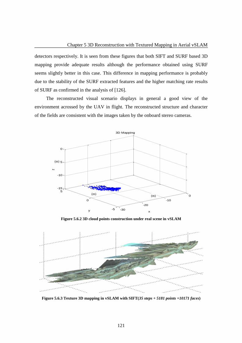
Chapter 5 3D Reconstruction with Textured Mapping in Aerial vSLAM
121
detectors respectively. It is seen from these figures that both SIFT and SURF based 3D
mapping provide adequate results although the performance obtained using SURF
seems slightly better in this case. This difference in mapping performance is probably
due to the stability of the SURF extracted features and the higher matching rate results
of SURF as confirmed in the analysis of [126].
The reconstructed visual scenario displays in general a good view of the
environment acrossed by the UAV in flight. The reconstructed structure and character
of the fields are consistent with the images taken by the onboard stereo cameras.
Figure 5.6.2 3D cloud points construction under real scene in vSLAM
Figure 5.6.3 Texture 3D mapping in vSLAM with SIFT(35 steps + 5181 points +10171 faces)
-30
-20
-10
0
-5
0
5-15
-10
-5
0
x
3D Mapping
y
z
(m)
(m) (m)

Chapter 5 3D Reconstruction with Textured Mapping in Aerial vSLAM
122
Figure 5.6.4 Texture 3D mapping in vSLAM with SURF(35 steps + 5670 points
+11162 faces)
Figure 5.6.5 Texture 3D mapping in vSLAM with SIFT without extra features added (35 steps +
3741 points +7305 faces)
Although, the above principle and algorithms for 3D reconstruction with texture
mapping are successful in this application, we also noted that it is possible to obtain a
distorted reconstruction when the plane at infinity acrosses the scene. This can result in
a failure. The solution to this is to use oriented projective geometry [68, 69], which is
not included here.
In addition, obtaining a perfect texture map may be very difficult in the case of
existing co-linearity of features in the image plane when matching the corresponding
image points to the triangulated surface. This can be caused by either distortion of
feature extraction, computing accuracy, or the independent calculation of Delaunay
Triangulation. The latter can yield a number of vertexes not consistent with those of
feature sequences in the image plane due to the elimination of co-linear points by

Chapter 5 3D Reconstruction with Textured Mapping in Aerial vSLAM
123
Delaunay Triangulation for reconstructing the surface of 3D space. RANSAC algorithm
was utilised to improve the inlier accuracy with the elimination of multiple matching,
which has effects on both data fusing and texture plating.
The mapping performance can also be affected by the number of corresponding
cloud points. An increased matching threshold can cause more error in obtaining
correspondences in the 3D calculation, but a smaller number of correspondences will
yield poorer visualisation in texture plating. The compromise currently conducted is to
refinine the correspondences through arranging sequences of features in order, and by
applying only the certain number of correspondences with the smallest Euclidean
distance for data fusing, while large amount of those is used for textured meshing.
5.6.3 Texture Mapping Based on Mosaic Imaging
As explained before, the initial intention of using mosaic imaging as a potential
texture was to apply it with vSLAM in textured mapping. The mosaicing finds its first
application in the case where a large scene is required. The second possible use could be
post processing for improving the quality of the reconstructed whole scene as a replay
after the real time flight. As a trial test, a run in a couple of frames is performed to
illustrate this purpose.
5.6.3.1 3D Reconstruction Textured with Mosaic Imaging
Mosaicing technology of constructing high resolution images that cover a wide
field of view using inexpensive equipment has won credits in various application areas.
Now, one of these is its theoretical capability of creating completely navigable
“virtualised” environments by using images from different camera views at different
frames. Based on these virtual environments, the 3D reconstruction of the whole scene
could be then created within one process, i.e., independently running vSLAM to obtain
a set of 3D reconstructed cloud points, storing both 3D points and 2D pixels of
landmarks in corresponding vectors, and then texture mapping conducting when
demanded in the end. To investigate this active research area, some empirical tests of
mapping with texture from mosaic aerial imaging (30 continuing frames shown in
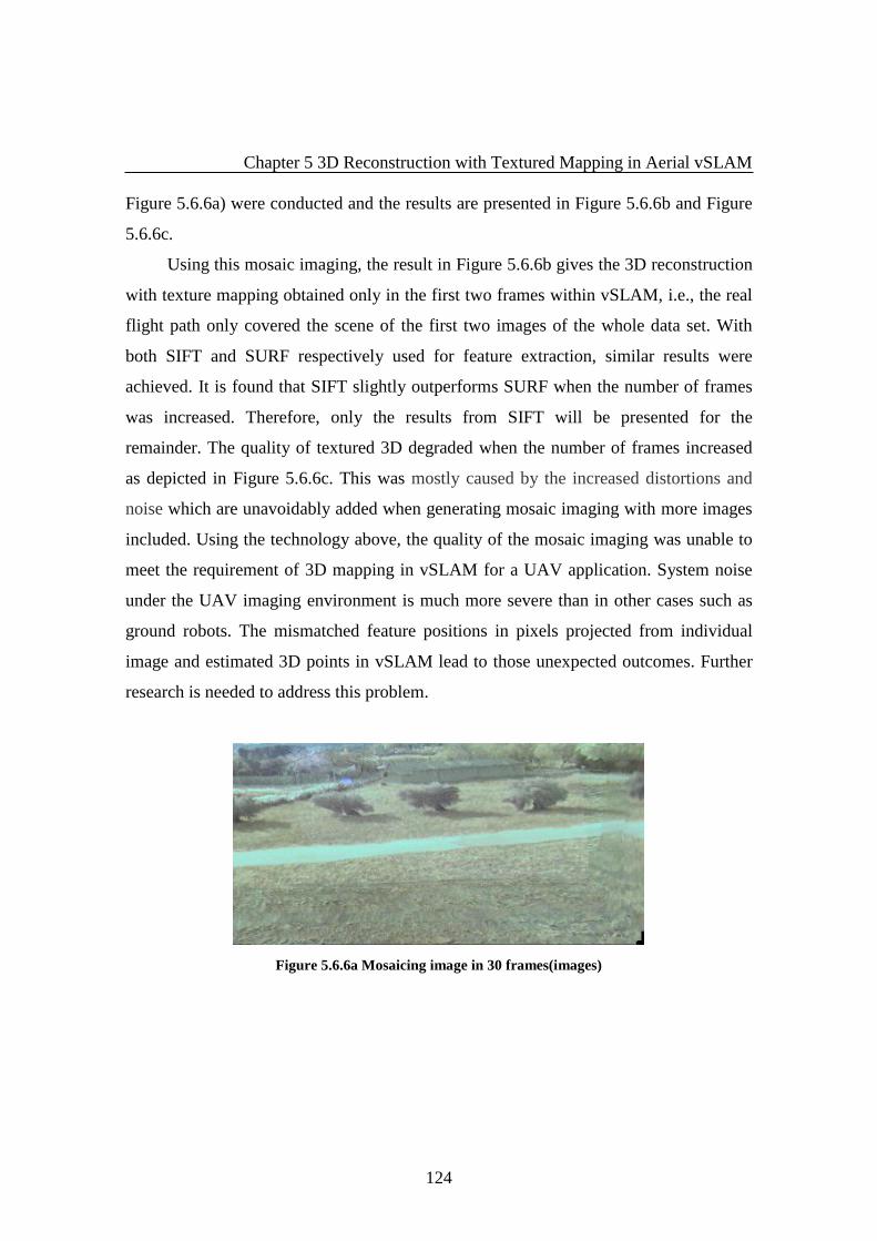
Chapter 5 3D Reconstruction with Textured Mapping in Aerial vSLAM
124
Figure 5.6.6a) were conducted and the results are presented in Figure 5.6.6b and Figure
5.6.6c.
Using this mosaic imaging, the result in Figure 5.6.6b gives the 3D reconstruction
with texture mapping obtained only in the first two frames within vSLAM, i.e., the real
flight path only covered the scene of the first two images of the whole data set. With
both SIFT and SURF respectively used for feature extraction, similar results were
achieved. It is found that SIFT slightly outperforms SURF when the number of frames
was increased. Therefore, only the results from SIFT will be presented for the
remainder. The quality of textured 3D degraded when the number of frames increased
as depicted in Figure 5.6.6c. This was mostly caused by the increased distortions and
noise which are unavoidably added when generating mosaic imaging with more images
included. Using the technology above, the quality of the mosaic imaging was unable to
meet the requirement of 3D mapping in vSLAM for a UAV application. System noise
under the UAV imaging environment is much more severe than in other cases such as
ground robots. The mismatched feature positions in pixels projected from individual
image and estimated 3D points in vSLAM lead to those unexpected outcomes. Further
research is needed to address this problem.
Figure 5.6.6a Mosaicing image in 30 frames(images)

Chapter 5 3D Reconstruction with Textured Mapping in Aerial vSLAM
125
Figure 5.6.6b 3D texture mapping on mosaic imaging in 2 frames(LHS: SIFT, RHS: SURF)
Figure 5.6.6c 3D texture mapping on mosaic imaging with SIFT (LHS: 5 frames, RHS: 10 frames)
5.7 Summary and Discussion
In this chapter, we have proposed a novel 3D mesh reconstruction methodology
combining the advantages of stereovision with the power of Delaunay triangulation of a
3D surface.
3D reconstruction with texture mapping provides a visualised way for vSLAM
map building for a on UAV application. The principle of the related techniques was
presented, with necessary details and process given for its application in this project.
Our technique computes locations of 3D points in the environment of landmarks based
on UAV position estimated with vSLAM in the global frame. By a number of extra
correspondences added based on homography transformation technique, and an
effective strategy of feature matching in consecutive frames, the smoothed and extended
view of the field is reconstructed. This vivid scenario is produced dynamically and
synchronised with the movement of the UAV.
Y(m)
Z(m)
Z(m)
Z(m)
Y(m)
Y(m) X(m)
X(m)
X(m)
Y(m)
X(m)
Z(m)
Chapter 5 3D Reconstruction with Textured Mapping in Aerial vSLAM
126
The texture mapping technique presented here provides a convincing performance
incorporating with vSLAM for a UAV application with a trade-off between sparse 3D
points and sufficient estimation accuracy, and yields substantial computational savings
to meet the requirement of real time application. The experimental results are
encouraging although the quality of images taken on the UAV platform is not of high
enough spatial resolution. The distortion caused by vibration is always severe, and the
estimation errors in vSLAM generally worsen the quality of 3D reconstruction.
As indicated by the newly developed applications, mosaic imaging has been an
attractive area of both commercial and military research. Therefore, we conducted an
investigation on mosaic imaging based on both geometric registration and photometric
registration to deal with contrast and luminosity changes with empirical tests carried
out. We expect the use of mosaic imaging to make a significant impact on textured 3D
reconstruction. The complete representation of static scenes resulting from mosaic
imaging frames in conjunction with an efficient representation for dynamic changes
aimed to provide a versatile environment for visualising, accessing, and analysing
information by large scene reconstruction in post processing of vSLAM.
The initial results show that this technique can be successful in providing quality
mosaic imaging by only using a limited number of frames within vSLAM process.
Unfortunately, because the distortion of images taken by moving on-board cameras is
always more severe than that taken by still cameras, and errors are unavoidably caused
by the image transformation, the quality of final mosaic imaging is degraded with
increasing number of frames. The quality of 3D reconstruction with the texture from
mosaic imaging is inevitably affected as well. Therefore, more efforts are required to
improve mosaic imaging techniques to meet the need of texture mapping for large
scenes in visual SLAM.

Chapter 6 Future Matching and Association in Airborne Binocular vSLAM
127
CHAPTER 6
Feature Matching and Association in Airborne Binocular
vSLAM
Feature matching and association are both indispensable parts in vision based
SLAM, especially in binocular systems. It is even more challenging when facing low
spatial resolution and blurred images taken from aerial vehicles. Hence, it is a must to
study it in detail to provide robust and validated methodologies in vSLAM scheme.
In this chapter, a SIFT algorithm was utilised as a features extraction algorithm in
the highly blurred aerial images, followed by the investigation of dense feature
matching and data association techniques with stereo camera imaging. Novel proposals
and tests are subsequently presented.
6.1 Overview of Image Features Matching and Association in vSLAM
One of most challenging and difficult issues of features matching and association
in SLAM, especially in visual SLAM is how to deal with the presence of dense and low
spatial resolution images. The efficient techniques of finding consistent
correspondences between two sets of features are absolutely necessary for the
successful operation of visual navigation.
It has been recognised that the emergence of visual SLAM (vSLAM) has huge
potential in terms of proving lower cost, richer informative and flexible sensing, capable
of operating with various previously unseen environments.
To fulfil this potential, system feasibility in the presence of various changes due to
both vehicles motion and environmental variation, must be solid. Those changes can
alter the effectiveness of feature matching and association.
Therefore, it is crucial to investigate the issues of feature matching and data
association in order to conduct robust, accurate and effective operation in visual SLAM.
This research endeavours to do so.
In stereo vision, feature matching is generally conducted between two camera
images, where the matches can be obtained through various approaches, such as cross
correlation with epipolar constraints or descriptor measurements as indicated in Chapter

Chapter 6 Future Matching and Association in Airborne Binocular vSLAM
128
3. The obtained matches can therefore be used for other purposes, such as triangulation
based 3D reconstruction in vSLAM.
Data association is the process of obtaining correct feature correspondences
between any image and previous existing features in store. There is the generality in the
nature of matching and association.
Data association relies on very discriminative feature matching as incorrect
matching leads to the selection of erroneous measurements. This easily occurs during
fast, or erratic motions, or in high altitude which largely affect the spatial resolution of
images captured onboard.
Traditionally, automatic image matching/geometry estimation falls into two
categories: direct and feature based. The former based on the assumption of fragile
'brightness constancy' is achieved through attempting to iteratively estimate the camera
parameters by minimising an error function based on the intensity difference in the
overlaping area. This is sometimes known as bundle adjustment [82, 83, 119].
Feature based methods are used to establish correspondences between lines or
other geometrical entities, which can be done, for example, by applying a normalised
cross-correlation of the local intensity values to match them, or by using distinctive
image descriptors. Improved matching speed and accuracy can be achieved through
epipolar constraint or RANSAC techniques. However, the application of epipolar
constraints usually requires online image rectification and a proper calibration. This
may not be feasible with aerial imaging, where the on air calibration is not practical.
This is part of the reason that it is more challenging to obtain good feature
matching and association in real time vSLAM for UAV application.
As depicted in Chapter 3, it is known that feature matching and association with
SIFT descriptors constructed on a histogram of spatial gradients representation to
provide a degree of invariance to the camera viewpoint, can be conducted with nearest
neighbour principle by the measurement of Euclidean distance as metrics of features
correlation based similarity. Given a good resolution in sparse images, this is usually an
efficient data association mechanism. However, in environments with highly dense
features, or low resolution images, this fails, as the high similarity and closeness of
feature imaging will largely blur the distinctive images.

Chapter 6 Future Matching and Association in Airborne Binocular vSLAM
129
Unfortunately, an effective solution to this problem is yet to be proposed.
Therefore, this work will attempt to find different alternative strategies incorporating
current techniques. One empirical effort is to reduce the disunity of features by
introducing the graph theory and matching approaches, and geometrically select
distinctive features in each image. We intended to take advantage of features’ pairwise
geometric information via graphs to find the right correspondence in the case of the
features are non-discriminative (e.g., points). When discriminative features are extracted
(e.g., interest points) then both the geometry and the individual properties of each
feature can be used. These matched features can be found more repeatedly and reliably.
When it comes to association, different methods will be employed, which will be
examined in subsequent sections.
We also demonstrate that the proposed matching approach and strategy shows the
improved performance of vSLAM in the presence of highly blurred aerial images.
6.2 Basic Notation and Terminology in Graph Theory
Graphs provide a natural structure to represent a wide array of data including
various real data structures in a wide variety of areas such as community networks,
biological diversity and computational workflows. This motivated the application of this
technique in imaging clustering for identifying distinctive landmarks in non-ideal
environment.
6.2.1 Graph Concept
In this section, we follow the references [120, 121].
Graph is used to characterise data geometry (e.g., manifold) and thus plays an
important role in data analysis.
Basically, a graph G = (V, E) consists of vertices and edges. Vertices V is the set
of points or nodes and the E is set of edges, which is also called lines or arcs of graph G.
E is defined E ⊂ V × V (or as in the literature E ⊂ [V]2).
The definition of order (or size) of a graph G is the number of vertices of G,
which is represented as |V | and the number of edges as |E|.
Two vertices u, v ∈ V in G are said to be adjacent or neighbours when they are
connected by an edge e ∈ E, this is denoted by e = (u, v). Undirected Edges have no

Chapter 6 Future Matching and Association in Airborne Binocular vSLAM
130
direction, and an undirected graph G contains only such types of edges. In directed
graph, all edges are assigned with directions. This makes the notation (u, v) and (v, u)
distinguished. Usually, the term 'arc' is for directed graph, and the 'edge' is for
undirected one. Undirected edges have end-vertices, and directed edges have a source
(head, origin) and target (tail, destination) vertices. A complete directed graph G = (V,
E) is named if an edge (u, u') ∈ E = V × V is always existing between any two vertices
in the graph.
There is information which can be held by vertices and edges of a Graph. A
labelled Graph is named if this information is a simple label (i.e., a number or name).
Otherwise, if more information is contained in vertices and edges, they are called vertex
and edge attributes. Consequently, the graph is called an attributed graph. More often,
this concept is given a specified definition by identifying between vertex-attributed (or
weighted graphs) and edge-attributed graphs.
A path between any two vertices u, u'∈ V is a non-empty sequence of k different
vertices < v0,v1,...,vk> where u = v0, u'=vk and (vi-1,vi)∈ E, i = 1, 2, . . . , k. At last, a
acyclic graph G is defined without cycles between its edges, no matter graph G is
directed or not.
There is an extended complex definition of Graph named Hypergraphs: E ⊆ 2V
(all subsets of elements of V), i.e., each edge (hyperedge) is a subset of vertices, such as
V={v1, v2, v3, v4, v5, v6, v7}, E={e1, e2, e3, e4}={{v1, v2, v3}, {v2, v3}, {v3, v5, v6}, {v4}}.
This is the fundamental motivation to construct hyper graph from camera images, in
order to obtain a feasible infrastructure for feature matching and data association with
stereo vision based vSLAM.
Figure 6. 2.1 Hypergraph representation

Chapter 6 Future Matching and Association in Airborne Binocular vSLAM
131
6.2.2 Graph Representation:
There are various ways in the representation of Graphs for graphs to be
computationally useful in practice. Although each way has its own pros and cons, the
different data structures for the convenient representation of graphs are summarised
below [120, 121]:
Adjacency list
Vertices are identified and stored as objects or records, and each vertex has
stockpile for a list of adjacent vertices, which provides a data structure of the
storage of additional data on the vertices.
Incidence list
Vertices and edges are identified and stored as objects or records. Each vertex
stores its incident edges, and each edge stores its incident vertices. The data
structure like this provides a feasible the storage of additional data on vertices
and edges.
Adjacency matrix
It is a two-dimensional matrix where the rows represent source vertices and
columns represent destination vertices. There is an external storage for data on
edges and vertices. Only the cost or attribute for one edge is to be stored
between each pair of vertices. This form of representation is usually applied in
graph matching.
Incidence matrix
It is also a two-dimensional Boolean matrix, in which the rows represent the
vertices and columns represent the edges. The entries indicate whether the vertex
at a row is incident to the edge at a column. Incidence matrix is also suitable in
graph matching application.
6.2.3 Dominating Set Concept
The proposed empirical approach of finding discriminative correspondences is
via Connected Dominate Set (CDS) in graph theory by considering the geometric
constraints in pixel or descriptor distance.
A dominating set of a graph is a subset of all the nodes S such that each node
is either in the dominating set or adjacent to some node in the dominating set. Here
is an example.
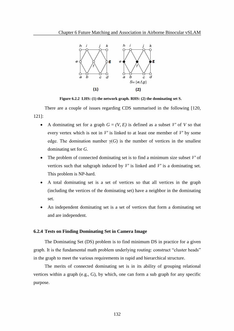
Chapter 6 Future Matching and Association in Airborne Binocular vSLAM
132
Figure 6.2.2 LHS: (1) the network graph. RHS: (2) the dominating set S.
There are a couple of issues regarding CDS summarised in the following [120,
121]:
A dominating set for a graph G = (V, E) is defined as a subset V′ of V so that
every vertex which is not in V′ is linked to at least one member of V′ by some
edge. The domination number γ(G) is the number of vertices in the smallest
dominating set for G.
The problem of connected dominating set is to find a minimum size subset V′ of
vertices such that subgraph induced by V′ is linked and V′ is a dominating set.
This problem is NP-hard.
A total dominating set is a set of vertices so that all vertices in the graph
(including the vertices of the dominating set) have a neighbor in the dominating
set.
An independent dominating set is a set of vertices that form a dominating set
and are independent.
6.2.4 Tests on Finding Dominating Set in Camera Image
The Dominating Set (DS) problem is to find minimum DS in practice for a given
graph. It is the fundamental math problem underlying routing: construct “cluster heads”
in the graph to meet the various requirements in rapid and hierarchical structure.
The merits of connected dominating set is in its ability of grouping relational
vertices within a graph (e.g., G), by which, one can form a sub graph for any specific
purpose.

Chapter 6 Future Matching and Association in Airborne Binocular vSLAM
133
For instance, given a connected dominating set S, spanning tree of G can be
generated, where S forms the set of non-leaf nodes of the tree. On the other hand, given
T as any spanning tree in a graph with more than two vertices, the non-leaf nodes of T
can therefore form a connected dominating set. It is then understood that, finding
minimum connected dominating sets is same as finding spanning trees with the
maximum possible number of leaves.
A fundamental problem of CDS is to divide a graph into clusters so that points in
different clusters are far apart.
The summarised elements for CDS utilised for the graph clustering in a sparse
data set:
Clustering. Given a set U of n objects labeled p1… pn, classify into coherent groups.
Distance function. Identity in numeric value specifying “closeness” of two
objects/vertices.
Before searching the minimum Dominating Set, usually the general domination
set can be found at first place, which is done via the greedy central algorithm [121] to
find DS:
1. First, select the vertex (or vertices) with the most neighbors (The vertex or vertices
with the largest degree), stop if a dominating set is made.
2. Otherwise, choose the vertices with the next largest degree, to see if it is done.
3. Do this iteratively until a dominating set is found.
The minimum dominating set is NP-hard problem in finding a minimum. An
existing efficient approximation algorithm Guha and Khuller Algorithm to find CDS,
1996[154], is the widely recognised pioneer.
Guha and Khuller Algorithm
Approach: Starting from the vertex with the highest degree to grow a tree T, at
each step, scan a node by adding all of its edges and neighbors to T. At the end, all non-
leaf nodes are in CDS.
Since Guha and Khuller algorithm appeared, a few other widely influencing ones
were developed such as:
• Das et al’s algorithm (1997) [155]
• Wu and Li’s algorithm (1999) [156]
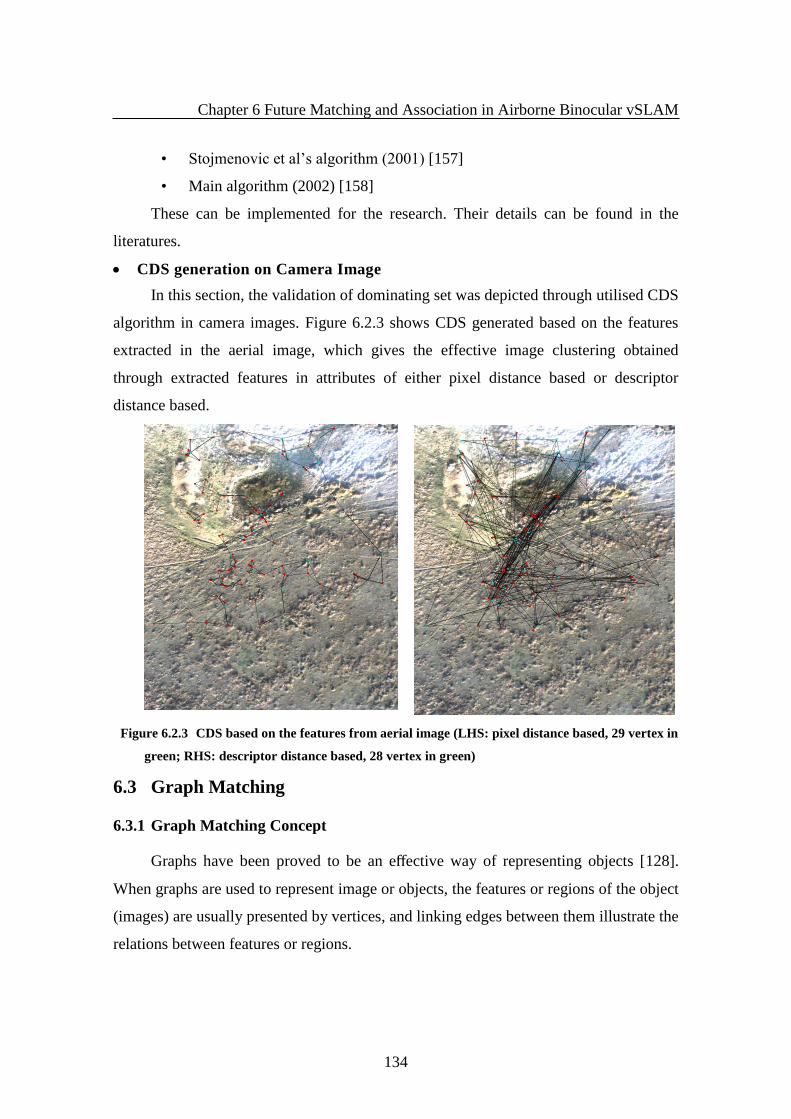
Chapter 6 Future Matching and Association in Airborne Binocular vSLAM
134
• Stojmenovic et al’s algorithm (2001) [157]
• Main algorithm (2002) [158]
These can be implemented for the research. Their details can be found in the
literatures.
CDS generation on Camera Image
In this section, the validation of dominating set was depicted through utilised CDS
algorithm in camera images. Figure 6.2.3 shows CDS generated based on the features
extracted in the aerial image, which gives the effective image clustering obtained
through extracted features in attributes of either pixel distance based or descriptor
distance based.
Figure 6.2.3 CDS based on the features from aerial image (LHS: pixel distance based, 29 vertex in
green; RHS: descriptor distance based, 28 vertex in green)
6.3 Graph Matching
6.3.1 Graph Matching Concept
Graphs have been proved to be an effective way of representing objects [128].
When graphs are used to represent image or objects, the features or regions of the object
(images) are usually presented by vertices, and linking edges between them illustrate the
relations between features or regions.
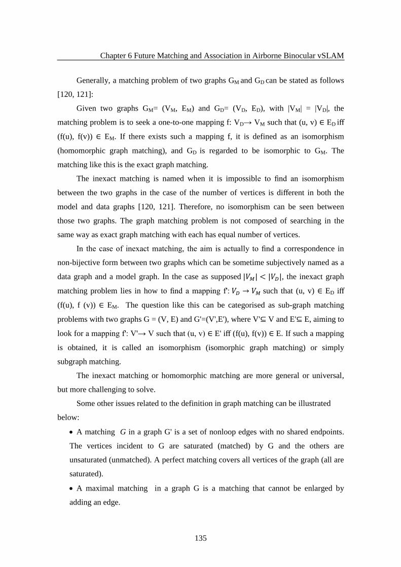
Chapter 6 Future Matching and Association in Airborne Binocular vSLAM
135
Generally, a matching problem of two graphs GM and GD can be stated as follows
[120, 121]:
Given two graphs GM= (VM, EM) and GD= (VD, ED), with |VM| = |VD|, the
matching problem is to seek a one-to-one mapping f: VD→ VM such that (u, v) ∈ ED iff
(f(u), f(v)) ∈ EM. If there exists such a mapping f, it is defined as an isomorphism
(homomorphic graph matching), and GD is regarded to be isomorphic to GM. The
matching like this is the exact graph matching.
The inexact matching is named when it is impossible to find an isomorphism
between the two graphs in the case of the number of vertices is different in both the
model and data graphs [120, 121]. Therefore, no isomorphism can be seen between
those two graphs. The graph matching problem is not composed of searching in the
same way as exact graph matching with each has equal number of vertices.
In the case of inexact matching, the aim is actually to find a correspondence in
non-bijective form between two graphs which can be sometime subjectively named as a
data graph and a model graph. In the case as supposed , the inexact graph
matching problem lies in how to find a mapping f': such that (u, v) ∈ ED iff
(f(u), f (v)) ∈ EM. The question like this can be categorised as sub-graph matching
problems with two graphs G = (V, E) and G'=(V',E'), where V'⊆ V and E'⊆ E, aiming to
look for a mapping f': V'→ V such that (u, v) ∈ E' iff (f(u), f(v)) ∈ E. If such a mapping
is obtained, it is called an isomorphism (isomorphic graph matching) or simply
subgraph matching.
The inexact matching or homomorphic matching are more general or universal,
but more challenging to solve.
Some other issues related to the definition in graph matching can be illustrated
below:
A matching G in a graph G' is a set of nonloop edges with no shared endpoints.
The vertices incident to G are saturated (matched) by G and the others are
unsaturated (unmatched). A perfect matching covers all vertices of the graph (all are
saturated).
A maximal matching in a graph G is a matching that cannot be enlarged by
adding an edge.

Chapter 6 Future Matching and Association in Airborne Binocular vSLAM
136
A maximum matching in a graph G is a matching of maximum size among all
matchings.
6.3.2 Empirical Investigation on Graph Matching
Recent decades have seen significant efforts by many researchers to develop a
number of graph matching algorithms based on several approaches. These can be
mainly summarised as genetic theory based and probability theory based [122]. These
have been utilised with additional techniques such as [122]:
Applying probabilistic relaxation to graph matching [129-132].
Applying the EM (Expectation Maximization algorithm) to graph matching [133-
134].
Applying decision trees to graph matching [135-136].
Graph matching using neural networks [137-139].
Graph matching using clustering techniques [140-141].
6.3.3 Proposed Graph Matching
Motivated by graph theory, we conceived the feature matching problem in camera
imaging as an ordinary graph matching problem. The features can be represented
through vertices as objects in the graph model. Therefore, the graph is generated within
an image and the corresponding feature matching will be executed as graph matching.
We look at utilising various techniques in order to find the solution of providing
and validating correct matching in highly dense feature images. Although, many graph
matching methods were utilised and tested during this research, we only show the
results of one of recent state of art graph transformation matching (GTM).
6.3.4 Graph Transformation
Most recent advanced graph matching algorithms adopt the general quadratic
programming formulation. It generally takes into consideration of both unary and
second-order terms which can represent the similarities in local appearance, and also the
geometric relationships of pairwise between the matches. It is an NP-hard problem.
Hence to make a compromise, the approximation solutions for sub-optimisation are
usually obtained by relaxing the original algorithm.
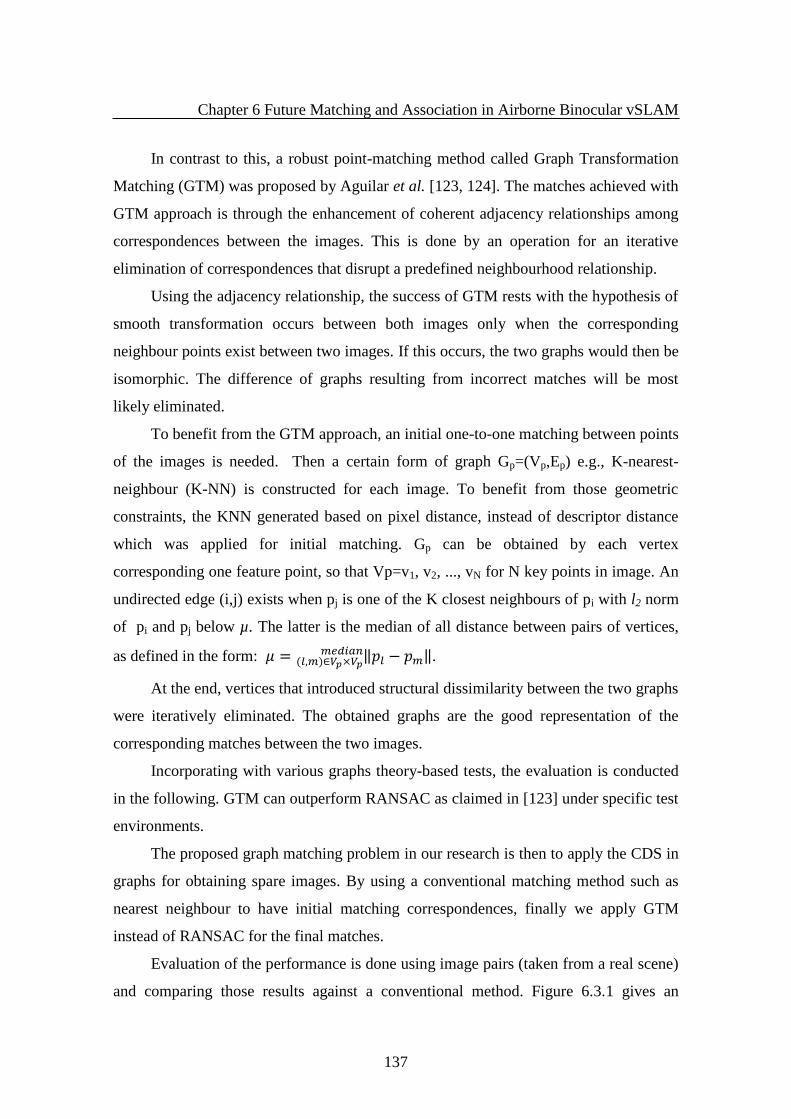
Chapter 6 Future Matching and Association in Airborne Binocular vSLAM
137
In contrast to this, a robust point-matching method called Graph Transformation
Matching (GTM) was proposed by Aguilar et al. [123, 124]. The matches achieved with
GTM approach is through the enhancement of coherent adjacency relationships among
correspondences between the images. This is done by an operation for an iterative
elimination of correspondences that disrupt a predefined neighbourhood relationship.
Using the adjacency relationship, the success of GTM rests with the hypothesis of
smooth transformation occurs between both images only when the corresponding
neighbour points exist between two images. If this occurs, the two graphs would then be
isomorphic. The difference of graphs resulting from incorrect matches will be most
likely eliminated.
To benefit from the GTM approach, an initial one-to-one matching between points
of the images is needed. Then a certain form of graph Gp=(Vp,Ep) e.g., K-nearest-
neighbour (K-NN) is constructed for each image. To benefit from those geometric
constraints, the KNN generated based on pixel distance, instead of descriptor distance
which was applied for initial matching. Gp can be obtained by each vertex
corresponding one feature point, so that Vp=v1, v2, ..., vN for N key points in image. An
undirected edge (i,j) exists when pj is one of the K closest neighbours of pi with l2 norm
of pi and pj below µ. The latter is the median of all distance between pairs of vertices,
as defined in the form: ‖ ‖ ∈ .
At the end, vertices that introduced structural dissimilarity between the two graphs
were iteratively eliminated. The obtained graphs are the good representation of the
corresponding matches between the two images.
Incorporating with various graphs theory-based tests, the evaluation is conducted
in the following. GTM can outperform RANSAC as claimed in [123] under specific test
environments.
The proposed graph matching problem in our research is then to apply the CDS in
graphs for obtaining spare images. By using a conventional matching method such as
nearest neighbour to have initial matching correspondences, finally we apply GTM
instead of RANSAC for the final matches.
Evaluation of the performance is done using image pairs (taken from a real scene)
and comparing those results against a conventional method. Figure 6.3.1 gives an
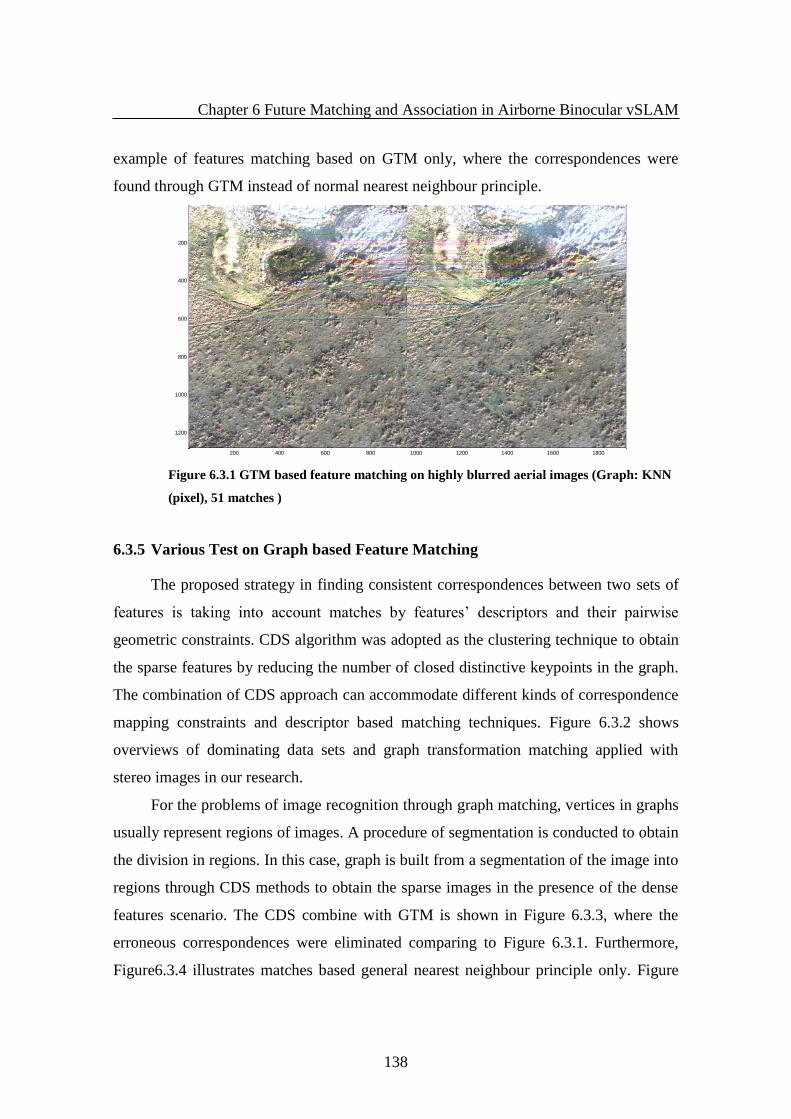
Chapter 6 Future Matching and Association in Airborne Binocular vSLAM
138
example of features matching based on GTM only, where the correspondences were
found through GTM instead of normal nearest neighbour principle.
Figure 6.3.1 GTM based feature matching on highly blurred aerial images (Graph: KNN
(pixel), 51 matches )
6.3.5 Various Test on Graph based Feature Matching
The proposed strategy in finding consistent correspondences between two sets of
features is taking into account matches by features’ descriptors and their pairwise
geometric constraints. CDS algorithm was adopted as the clustering technique to obtain
the sparse features by reducing the number of closed distinctive keypoints in the graph.
The combination of CDS approach can accommodate different kinds of correspondence
mapping constraints and descriptor based matching techniques. Figure 6.3.2 shows
overviews of dominating data sets and graph transformation matching applied with
stereo images in our research.
For the problems of image recognition through graph matching, vertices in graphs
usually represent regions of images. A procedure of segmentation is conducted to obtain
the division in regions. In this case, graph is built from a segmentation of the image into
regions through CDS methods to obtain the sparse images in the presence of the dense
features scenario. The CDS combine with GTM is shown in Figure 6.3.3, where the
erroneous correspondences were eliminated comparing to Figure 6.3.1. Furthermore,
Figure6.3.4 illustrates matches based general nearest neighbour principle only. Figure
200 400 600 800 1000 1200 1400 1600 1800
200
400
600
800
1000
1200

Chapter 6 Future Matching and Association in Airborne Binocular vSLAM
139
6.3.5 presents the result of using GTM as refining role after nearest neighbour (NN)
principle adopted given comparison to the matching with RANSAC as presented in
Figure 6.3.6. Due to the limited resolution of image, results look quite similar except
more matches can be obtained with RANSAC given the appropriate settings. There is
one thing worth mentioning that matches with GTM are sparser and uniformly
distributed cross images, from which depth calculation can benefit later. Please note that
the graph generation here is based on pixels distance instead of feature descriptors. As
GTM is a geometrical transformation, the descriptor-based graph/CDS could not yield
good matches. But descriptor based graph/CDS can be applied with NN principle alone
without GTM being included.
Initialization
1st
image 2nd
image
Features
extraction
Features
extraction
Graph Generation Graph Generation
CDS? CDS?
Yes Yes
No No
Dominating Sets Dominating Sets
Graph
Matching NN Matching
Figure 6.3.2 Dominating data sets and graph matching in stereo images

Chapter 6 Future Matching and Association in Airborne Binocular vSLAM
140
Figure 6.3.3 CDS+GTM based feature matching on highly blurred aerial images (Graph:
KNN (pixel), 12 matches )
Figure 6.3.4 General Nearest Neighbour (NN) principle based feature matching on highly
blurred aerial images (110 matches )
200 400 600 800 1000 1200 1400 1600 1800
200
400
600
800
1000
1200
200 400 600 800 1000 1200 1400 1600 1800
200
400
600
800
1000
1200
Chapter 6 Future Matching and Association in Airborne Binocular vSLAM
141
Figure 6.3.5 NN+GTM based feature matching on highly blurred aerial images (Graph:
KNN (pixels); 67 matches )
Figure 6.3.6 NN+RANSAC based feature matching on highly blurred aerial images (80
matches )
6.3.6 Use of Graph Theory in vSLAM
Aiming to overcome the non-distinctive landmarks in highly blurred images, we
carried out an experimental study on graph theory-based matching utilised with
vSLAM. The data sets used were the same as the one in a later Chapter 7 used for the
investigation on C-vSLAM.
200 400 600 800 1000 1200 1400 1600 1800
200
400
600
800
1000
1200
200 400 600 800 1000 1200 1400 1600 1800
200
400
600
800
1000
1200

Chapter 6 Future Matching and Association in Airborne Binocular vSLAM
142
The comparison conducted is with non-graph theory matching schema using
conventional Euclidean distance based Nearest Neighbor principle.
Conventional vSLAM
For the purpose of comparison, the estimation in aerial vSLAM was conducted
with only Feature based Euclidean distance with Nearest Neighbour principle, which is
presented in Figure 6.3.7a.
Figure 6.3.7a vSLAM with conventional matching strategy (Red-INS; Cyan- SLAM)(above:
Trajectory in 3 dimension, below: Error comparison)
Test on CDS in vSLAM
This test was carried out for the validation of utilising CDS in vSLAM during the
feature matching process. The obtained results in Figure 6.3.7b show that the estimation
0 20 40 60 80 100 120 140 1600
200
400
600Position X error !
Err
o
Time step
SLAM
INS
0 20 40 60 80 100 120 140 1600
200
400
600Position Y error !
Err
o
Time step
SLAM
INS
0 20 40 60 80 100 120 140 1600
200
400
600Position Z error !
Err
o
Time step
SLAM
INS
0 20 40 60 80 100 120 140 1600
200
400Position overall error !
Err
o
Time step
SLAM
INS

Chapter 6 Future Matching and Association in Airborne Binocular vSLAM
143
for vSLAM can be improved with integration of CDS, compared with the results in
Figure 6.3.7a.
Figure 6.3.7b vSLAM with CDS in matching strategy (Red-INS; Cyan- SLAM) (above: Trajectory
in 3 dimension, below: error comparison with INS)
Test on GTM in vSLAM
This test was carried out for the validation of utilising GTM in vSLAM during the
feature matching process. The results in Figure 6.3.7c show that the overall accuracy of
estimation for vSLAM can also be improved using GTM in feature matching
procedures, compared with the results in Figure 6.3.7a.
In addition, the possible use of CDS and GTM is not shown here, even we are
confident that they can definitely improve overall performances of estimation in
0 20 40 60 80 100 120 140 1600
200
400
600Position X error !
Err
o
Time step
SLAM
INS
0 20 40 60 80 100 120 140 1600
50
100Position Y error !
Err
o
Time step
SLAM
INS
0 20 40 60 80 100 120 140 1600
200
400
600Position Z error !
Err
o
Time step
SLAM
INS
0 20 40 60 80 100 120 140 1600
200
400Position overall error !
Err
o
Time step
SLAM
INS

Chapter 6 Future Matching and Association in Airborne Binocular vSLAM
144
vSLAM. This use may not be practical due to computation cost on graph generation in
real time under normal conditions.
Figure6.3.7c vSLAM with GTM in matching strategy (Red-INS; Cyan- SLAM) (above: Trajectory
in 3 dimension, below: error comparison with INS)
6.4 Novel Proposals of Data Association Schema
The updating navigation relies on how to decide if the external observation
corresponds to a previous existing mapped landmark or to a newly captured different
landmark. The decision made is rooted in data association technologies.
In visual SLAM the widely used approach for data association is based on the
matched features. Matching the observed feature points to the predicted ones is usually
done in a "pointwise" manner. This methodology can work reasonably well on sparse
features. Unfortunately, due to the high volume of feature vectors being tracked in
SLAM, especially in the sensing of camera imaging, the well-established data
association techniques in the multiple target tracking of "point" targets e.g., joint
0 20 40 60 80 100 120 140 1600
200
400
600Position X error !
Err
o
Time step
SLAM
INS
0 20 40 60 80 100 120 140 1600
100
200
300Position Y error !
Err
o
Time step
SLAM
INS
0 20 40 60 80 100 120 140 1600
200
400
600Position Z error !
Err
o
Time step
SLAM
INS
0 20 40 60 80 100 120 140 1600
200
400Position overall error !
Err
o
Time step
SLAM
INS

Chapter 6 Future Matching and Association in Airborne Binocular vSLAM
145
probability data association (JPDA), multiple hypothesis tracking (MHT) [4], or
multiform assignment algorithm [15] do not provide effectiveness.
In existing approaches for camera imaging, for an example of feature extraction
by SIFT (see chapter 3), the most acceptable one is still based on NN principle
incorporating with the Euclidean distance between SIFT descriptors expressed as E =
(di − dj)(di − dj)T , where di and dj are the SIFT descriptors. In this case, the landmark of
the map that minimises the distance E is regarded as the correct data association subject
to whenever the distance E is below a certain threshold. If the condition is met in this
case, the two landmarks are considered to be the same. Otherwise, a new landmark is
created.
As explained in chapter 3, SIFT descriptor is invariant to slightly viewpoints and
distance changing, i.e., features’ SIFT descriptor remains quite similar. However, when
significant changes happened, the difference in the descriptor is remarkable and the
check using the Euclidian distance is likely to produce an incorrect data association.
This is an issue facing data association within vSLAM. There is no perfect solution yet,
but different strategies may be suitable for utilisation in certain circumstances.
6.4.1 Classification Based Data Association Strategy
We propose an alternative way in the data association with the context of SIFT
features. The method was proposed and utilised independently although it is later seen
the similarity in [127]. The idea is conceptually introduced from pattern classification.
We regard the aggregation of re-observations of a landmark (by stereo cameras) in
vSLAM can be considered as class Ci modelling of a landmark with attributes of
previously estimated location, error covariance ∑i (256x256), the mean µi (256x1) of its
descriptor. The classification obtained using a new observation measured in descriptor
as a pattern dj to assign in the class Ci. This is done by comparing dj with the mean µi of
class Ci via Mahalanobious distance or Euclidean distance. Within the presetting
criteria, the decision can then be made if the association exists.
Having multiple observations of the same landmark from several view points
along consecutive frames, we extract SIFT features from stereo images as different
elements of class Ci, and we store them. Whenever a new landmark dj is found, by using
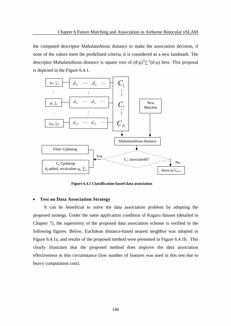
Chapter 6 Future Matching and Association in Airborne Binocular vSLAM
146
the computed descriptor Mahalanobious distance to make the association decision, if
none of the values meet the predefined criteria, it is considered as a new landmark. The
descriptor Mahalanobious distance is square root of (d-µ)T∑
-1(d-µ) here. This proposal
is depicted in the Figure 6.4.1.
Test on Data Association Strategy
It can be beneficial to solve the data association problem by adopting the
proposed strategy. Under the same application condition of Kagaru dataset (detailed in
Chapter 7), the superiority of the proposed data association scheme is verified in the
following figures. Below, Euclidean distance-based nearest neighbor was adopted in
Figure 6.4.1a, and results of the proposed method were presented in Figure 6.4.1b. This
clearly illustrates that the proposed method does improve the data association
effectiveness in this circumstance (low number of features was used in this test due to
heavy computation cost).
Figure 6.4.1 Classification based data association
µi, ∑i
Initiali
µN, ∑N
µ1, ∑1
New
Matches
Filter Updating
Mahalanobious distance
No
No
Yes
Cj Updating
dj added, recalculate µj, ∑j
Store in CN+1
Cj associatedd?

Chapter 6 Future Matching and Association in Airborne Binocular vSLAM
147
Figure 6.4.1a Estimation of vSLAM with conventional association methods (above: Trajectory in 3
dimension, below: Error comparison)

Chapter 6 Future Matching and Association in Airborne Binocular vSLAM
148
Figure 6.4.1b Estimation of vSLAM with proposed association strategy (above: Trajectory in 3
dimension, below: Error comparisons)
6.4.2 Graph Based Data Association Strategy
Another proposal in terms of Graph based data association with the context of
SIFT features schema is given in this section. Taking into consideration of both
geometric information in graphs and photometric perception in SIFT descriptor, we
utilised hyper graph transformation matching (HGTM) algorithm within conventional
data association method in stereo aerial images based visual SLAM. The same Kagraru
data sets as above section are used. The graph is described in hyper graph concept,
where each vertex is attributed by pair of matches obtained by coarse matching through
conventional data association scheme. The graph is then to be formed by Euclidean
distance of those vertexes. This HGTM based proposal is presented in Figure 6.4.2.
The empirical study will be given next.

Chapter 6 Future Matching and Association in Airborne Binocular vSLAM
149
Test on Data Association Strategy
The test conducted here is to show the benefit of this proposed association
strategy. A group of Figures show the superiority of the proposed data association
scheme. Under same settings, the adoption of graph transformation in data association
presented better performance in terms of overall estimation accuracy. It outperforms
INS, while conventional NN based is inferior to INS. These results were obtained with
dense number of features in SLAM, where the proposed data association strategy show
its advantages.
Figure 6.4.2 HGTM based data association
Stored
Matches
New
Matches
Filter Updating Continue
Associated?
Corse Association
Hyper Graph Generation
HGTM
Yes No
Initialisation

Chapter 6 Future Matching and Association in Airborne Binocular vSLAM
150
Figure 6.4.2a Estimation of vSLAM with conventional association methods (above: Trajectory in 3
dimension, below: Error comparisons)
0 20 40 60 80 100 120 140 1600
50
100
150Position X error !
Err
o
Time step
SLAM
INS
0 20 40 60 80 100 120 140 1600
50
100
150Position Y error !
Err
o
Time step
SLAM
INS
0 20 40 60 80 100 120 140 1600
200
400
600Position Z error !
Err
o
Time step
SLAM
INS
0 20 40 60 80 100 120 140 1600
100
200Position overall error !
Err
o
Time step
SLAM
INS

Chapter 6 Future Matching and Association in Airborne Binocular vSLAM
151
Figure 6.4.2b Estimation of vSLAM with proposed GTM association strategy (above: Trajectory in
3 dimension, below: Error comparisons)
6.5 Summary and Discussion
In this chapter, methodologies and validation of alternative feature matching and
association utilised in the vSLAM were presented.
An in-depth investigation was given of the graph-based features matching
methods taking consideration of the mixture models of information in SIFT descriptor
and geometrical arrangement of pixels represented by graph nodes and their structural
relationships (consistency).
To obtain robust data association in camera stereo image based visual SLAM, two
novel data associations were proposed. One is based on Mahalanobi distance calculation
in a classification concept. The second one is hyper graph transformation based.
Their superiority was verified by a number of tests conducted on the very low
resolution images sets, which show that both of them outperform the conventional
Euclidean distance-based nearest neighbour principle in this case. They are novel in the
literature. The latter has not been seen from reviewed literature where vSLAM in stereo
vision matching association was utilised.
Other merits of HGMT based association can run even quicker given appropriate
number selected correspondences. While the classification based method has advantages
in the situation of lower number of features, the computation cost prevents its utilisation
with dense features in vSLAM.
0 20 40 60 80 100 120 140 1600
50
100
150Position X error !
Err
o
Time step
SLAM
INS
0 20 40 60 80 100 120 140 1600
50
100Position Y error !
Err
o
Time step
SLAM
INS
0 20 40 60 80 100 120 140 1600
50
100
150Position Z error !
Err
o
Time step
SLAM
INS
0 20 40 60 80 100 120 140 1600
50
100Position overall error !
Err
o
Time step
SLAM
INS

Chapter 7 Collaborative Navigation of UAVs with vSLAM
152
CHAPTER 7
Collaborative Navigation of UAVs with vSLAM
In this chapter, the investigation of various collaborative techniques for multiple
UAVs is presented to achieve the objectives of C-vSLAM based navigation.
Navigation for multiple air vehicles is the central and most challenging part in our
research. Here, we are going to address the feasible solution of distributed and
decentralised cooperative visual SLAM for utilisation within UAVs. The proposal of
fusion strategy with covariance intersection technique for multiple UAVs equipped with
stereo vision camera system is given.
This experimental study utilised a decentralised cooperative data fusion strategy
with stereo vision camera systems. The collaborative estimation was implemented with
an information filter and covariance intersection algorithm to investigate potential
improvements in robustness to noise and accuracy of location, when compared to a
single UAV employing vSLAM alone.
The study and research work then focused on methodologies in collaborative
visual SLAM for multiple UAVs navigation incorporating novel HGTM data
association method. A comparative analysis on the proposed feasible strategies and
algorithms in cooperation of multiple UAVs is given.
7.1 Overview
Simultaneous localisation and mapping (SLAM) [1, 2, 28] has theoretically
reached a sufficient maturity, which, thereafter, leads to multiple vehicles or multi-
sensors cooperative SLAM (C-SLAM) [7, 8]. It is believed that the use of multiple co-
operating vehicles for a mission such as mapping or exploration has many advantages
over single-vehicle architecture [7, 8]. To achieve this, the remaining challenges for
improving the accuracy and robustness of the collaborative filter estimation
performance must be overcome to enable the application of C-SLAM. The physical
distribution of the co-operating vehicles induces the need to deal with the processing
observation information from physically distributed nodes sensing the environment in
different perspectives. There is therefore the requirement to estimate the specific states
Chapter 7 Collaborative Navigation of UAVs with vSLAM
153
of interest by relating multi-observation to the states through system process and
environment models. To achieve this, the high performance data-fusion algorithm
becomes a crucial component of the cooperative system to meet performance
requirement.
The mechanism and current preferred enabler for SLAM, Extended Kalman Filter
(EKF)[4] is still valuable. Its feasible implementation embedded in SLAM during local
estimation procedure is a plus. Information Filter displays properties that would appear
to make it a more optimal solution. Its correction form has characteristics which
implicates it would be more suitable for the multi-sensor/ platform data fusion
application task as analysed in Chapter 4.
Under the application of decentralised SLAM on Unmanned Air Vehicle (UAV)
platforms in 6 DoF rather than on 3D ground robots, the highly non-linear INS model
together with camera observation models tends to cause severe problems on the
condition and convergence of the filtering. Furthermore, the possible aggressive
dynamics e.g., excessive roll rates can easily affect sensing directivity, and both flight
speeds and vibration will naturally deteriorate the imaging quality and quantity of the
landmarks observed. Apart from above, the excessive vibrations also worsen the inertial
drift rates, let alone memory and computational burden due to the massive state vector
covering both vehicles and landmarks observed.
In the decentralised C-SLAM, most of the data fusion challenges come from the
cooperation among multiple UAVs. Information filter can make multi-sensor data
fusion easier for the information gain to be shared by different cooperative nodes based
on consistent feature of observation enhancement provided that the architecture of states
and its uncertainty are distributed equally in different nodes. The estimation of the states
is carried out by combining states of platforms and landmarks in joined updating
manner. Common shared observation of landmarks is augmented in different position of
the states vector on different nodes. The only contribution to increase the estimation
accuracy comes from those observed landmarks that are now or ever observed by
corresponding UAV peers. The updating through those commonly shared observations
cannot be normally fulfilled in batch under platforms distribution. The application of
fully connected decentralised C-vSLAM can overcome this issue and implemented it.

Chapter 7 Collaborative Navigation of UAVs with vSLAM
154
A decentralised system is required to process all data locally and therefore no
central processing. Under this architecture, given fully connected network, C-vSLAM
will have the same system model residing on each node. Hence, the state vector and
corresponding state covariance that determine the uncertainty of vSLAM will be
identical on all nodes in the network. This makes information assimilation easy. At the
same time, it will still have advantage in modularity, survivability, flexibility and
extensibility [7, 8].
Fully connected decentralised cooperative vSLAM have inherent limitations due
to communication constraints. The communication among the nodes in high or full rates
as demanded in centralised data fusion prevents it from application in the large scale
network. To solve this problem with an effective communication in limited bandwidth,
only the necessary map information of the corresponding shared landmarks and their
relative uncertainty are communicated among distributed nodes. Covariance intersection
[51] provides a flexible and scalable fashion for the network of platforms to exchange
information and coordinate activities during decentralised data fusion. We take
advantages of both information filter and covariance intersection technique in
distributed and decentralised cooperative vSLAM (C-vSLAM).
The external sensors on the individual platform for our C-vSLAM are the
binocular vision system formulated by two cameras to obtain space coordinates of the
landmarks drawn from computer vision.
The experiments are carried out based on the system model in Chapter 4 with the
expectation of the remarkable achievements in decentralised data fusion in C-vSLAM.
7.2 Covariance Intersection (CI)
In the decentralised SLAM architecture, among nodes or platforms in network,
there is a need to exchange map information of landmarks determined through local
filtering. Map information received by one node from other heterogeneous nodes has to
be fused and optimised with its local map to have a better estimate for navigation. One
effective method discovered is CI which is a fusion algorithm for combining two or
more estimates (e.g., state estimates and sensor measurements from different platforms)
[33, 51] when the correlation among those estimates are unknown. As in distributed

Chapter 7 Collaborative Navigation of UAVs with vSLAM
155
SLAM, the measurements come from different platforms. In terms of algorithmic
performance alone, CI can provide a solution for the data fusion of unknown
correlations from distributed multiple platforms subject to nonuniform resident system
models – requirement of decentralised C-vSLAM. Here, only the common observed
features are available for fusion in order to contribute to the improvement of the overall
estimation of state accuracy cross the multiple UAV platforms. Therefore, if powered
by computer vision algorithms to provide accurate identification and positioning of
corresponding features for data fusion, CI presents itself as a potential primary
candidate for the task of data fusion in specific role of decentralised C-SLAM.
The CI algorithm, and its underpinning mathematical principles presented by
Simon Julier and Jeffrey K. Uhlmann [33, 51], is introduced as follows:
In the generic form of CI, the algorithm utilises a convex combination of mean
and covariance estimates representing information (inverse covariance) space. The
approach is intuitively motivated from a geometric interpretation of the Kalman filter
equations [33, 51]. Suppose random variables a and b with corresponding error
covariance aaP and
bbP written in the form {a,aaP } and {b,
bbP }, the fused variable c and its
corresponding error covariance ccP are in the form {c,
ccP } can be defined as:
111 )1( bbaacc PPP
(7.1) bPaPcP bbaacc111 )1(
The weighting parameter 0≤ 1 is used to optimise the weights assigned to a and
b with respect to different performance criteria such as minimising the trace or the
determinant of ccP by the cost function,
])1(det[
1min)det(min
11
bbaa
ccPP
PJ
(7.2)
It is clear that the inverse form aaP 1 , bbP 1 and ccP 1 are exactly the information
form of the covariance. This is extracted via the common features shared cross the
UAVs, as captured via the feature matching (in simulation model, for comparison, it
was utilised through an index). The inverse information covariance ccP 1 is optimised

Chapter 7 Collaborative Navigation of UAVs with vSLAM
156
through weighting parameter obtained in (7.2), which is then used as the replacement
for the corresponding original value. This adjustment makes the information filter more
optimal in the data fusion procedure.
7.3 Decentralised Cooperative Aerial vSLAM
This section presents our research on distributed UAV cooperative vSLAM and
its location and map accuracy comparing with single vSLAM. Performance in terms of
error comparison and robustness is demonstrated. Relative merits are discussed to
conclude this research.
7.3.1 State Structure in C-vSLAM
For fully connected cooperative vSLAM, the overall system has the same model
as a centralised architecture. The states vector and corresponding error covariance are
the joint optimised states and covariance extended from single UAV solution proposed
as in Chapter 4. Therefore, in cooperative multi-UAV vSLAM problems, the estimated
states are the jointed optimizated vectors of position, velocity and altitude of each
vehicle with respect to corresponding individual observation to the environment.
The general discrete time state transition equation for non-linear system in the
multiple UAVs case can be conceptually written as [62]:
),(
)(),( 1111
kkk
kkkkk
vXhY
wXgUXfX
f (:) is the discrete time state transition function, at time step k , kX is the state vector
with the same elements presented for UAV in Chapter 4, kw is additive process noises
with )( kXg as time variant weight, kY is the observation made at time k by UAVs at
each platform, kv is additive observation noises. The objective of the cooperative data
fusion is, then, to estimate kX using available observation kY independently based on
individual platform with the sharing information through communication. Each

Chapter 7 Collaborative Navigation of UAVs with vSLAM
157
platform will have individual state structure as
i
kl
i
k
i
k
kuavi
ki
m
m
m
X
X
,
,2
,1
,
,
where l denotes the
number of observed landmarks in single ith
UAV up to navigation frame k. Individual
landmark is denoted as m in 3 dimensions. The main merit of the decentralised C-
vSLAM is the flexibility of data fusion and communication in practice. By adopting CI
algorithm, only the individual state would be involved in data fusion, therefore, the cost
of system computation and communication would be ideally reduced to minimum for
decentralised platforms.
7.3.2 Experimental Results in Simulation
To depict C-vSLAM with data fusion via CI, two sets of results are shown in
Figure7.3.1 and Figure7.3.2 - demonstrating against randomly generated landmarks
based on a cooperative formation of two UAVs. As can be seen from these Figures, the
proposed schema produced impressive results with enhanced performance under the
specified test conditions. A processing noise deviation magnitude of w and a
measurement deviation m for a run of up to 360 time steps are given.
Figure7.3.1 presents an example of this schema. Exceptional results were obtained
in C-vSLAM (‘cUAV’) over single SLAM (‘sUAV’), with magnitude of processing
noise at w =0.5, observation error deviation at
m = 6 pixels. With a compacted, smaller
error covariance distribution, C-vSLAM has achieved less estimation errors than single
SLAM in all dimensions.
This same superiority in performance was also evident in Figure7.3.2 when the
scenario’s conditions were modified to accommodate an increase in the noise
environment withm of up to 10 pixels, and the processing noise set to
w =0.5 as before.
Figure7.3.2 clearly shows that even with the effect of increased observation error, C-
vSLAM integrated with CI will outperform a single vSLAM system that suffers from
the same severe divergence of the INS. This provides further evidence to illustrate that
C-vSLAM has advantages through improved filtering performance, even under
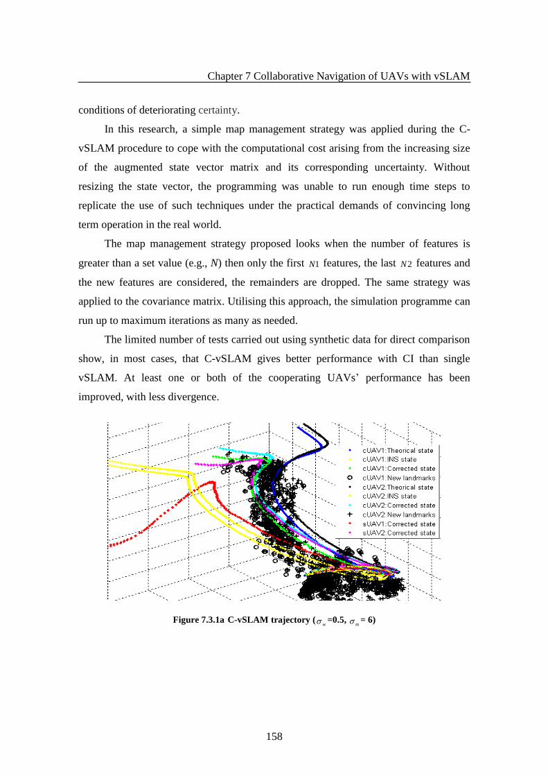
Chapter 7 Collaborative Navigation of UAVs with vSLAM
158
conditions of deteriorating certainty.
In this research, a simple map management strategy was applied during the C-
vSLAM procedure to cope with the computational cost arising from the increasing size
of the augmented state vector matrix and its corresponding uncertainty. Without
resizing the state vector, the programming was unable to run enough time steps to
replicate the use of such techniques under the practical demands of convincing long
term operation in the real world.
The map management strategy proposed looks when the number of features is
greater than a set value (e.g., N) then only the first 1N features, the last 2N features and
the new features are considered, the remainders are dropped. The same strategy was
applied to the covariance matrix. Utilising this approach, the simulation programme can
run up to maximum iterations as many as needed.
The limited number of tests carried out using synthetic data for direct comparison
show, in most cases, that C-vSLAM gives better performance with CI than single
vSLAM. At least one or both of the cooperating UAVs’ performance has been
improved, with less divergence.
Figure 7.3.1a C-vSLAM trajectory (w =0.5,
m = 6)

Chapter 7 Collaborative Navigation of UAVs with vSLAM
159
Figure 7.3.1b Error comparison of c-vSLAM (blue) and single vSLAM (red) (
w =0.5, m = 6)
Figure 7.3.1c Corresponding 2σ points of covariance 3D distribution for UAV1(
w =0.5, m = 6)
Figure 7.3.1d Corresponding 2σ points of covariance 3D distribution for UAV2(w =0.5,
m = 6)
-0.1
-0.05
0
0.05
0.1
-0.1
-0.05
0
0.05
0.1-0.1
-0.05
0
0.05
0.1
East(m)
2-Sigma position error covariance of UAV1-C(green)/S(blue)
North(m)
Dow
n(m
)
-0.1
-0.05
0
0.05
0.1
-0.2
-0.1
0
0.1
0.2-0.2
-0.1
0
0.1
0.2
East(m)
2-Sigma position error covariance of UAV2-C(cyan)/S(black)
North(m)
Dow
n(m
)

Chapter 7 Collaborative Navigation of UAVs with vSLAM
160
Figure 7.3.2a C-vSLAM trajectory (w =0.5,
m = 10)
Figure 7.3.2b Error comparison of C-vSLAM (blue) and single vSLAM (red) (w =0.5,
m = 10)
Figure 7.3.2c Corresponding 2σ points of covariance 3D distribution for UAV1 (w =0.5,
m = 10)
0 100 200 300 4000
1020
C(blue)/S(red)UAV1 Error x
0 100 200 300 4000
510
C(blue)/S(red)UAV2 Error x
0 100 200 300 4000
1020
C(blue)/S(red)UAV1 Error y
Err
or(m
)
0 100 200 300 4000
1020
C(blue)/S(red)UAV2 Error y
Err
or(m
)
0 100 200 300 4000
510
C(blue)/S(red)UAV1 Error z
0 100 200 300 4000
5C(blue)/S(red)UAV2 Error z
0 100 200 300 4000
510
C(blue)/S(red)UAV1 overall Error
Time Steps
0 100 200 300 4000
510
C(blue)/S(red)UAV2 overall Error
Time Steps
-0.2
-0.1
0
0.1
0.2
-0.2
-0.1
0
0.1
0.2-0.2
-0.1
0
0.1
0.2
East(m)
2-Sigma position error covariance of UAV1-C(green)/S(blue)
North(m)
Dow
n(m
)

Chapter 7 Collaborative Navigation of UAVs with vSLAM
161
Figure 7.3.2d Corresponding 2σ points of covariance 3D distribution for UAV2 (w =0.5,
m = 10)
7.4 Experiments conducted for C-vSLAM with Real Data Sets
The real dataset used for the test of decentralised C-vSLAM is taken from a single
flight generated by multiple paths of a remote control UAV (Figure 7.4.1) above
outdoor field, in Kagrau, Queensland, Australia [125].
The selected overlapping trajectories were allocated to independent UAV models
which acted as two UAVs going through the area at the same time. According to the
real flight, each UAV was equipped with inertial sensors (IMU), GPS and a pair of
stereo Grey Flea2firewire camera. It is a downward facing camera, lengthwise in the
fuselage with baseline of 0.75m with a resolution of 1280x960, 6mm focal length lenses
and BayerGR8 image format. After post processing of the raw data obtained from the
real flight, and synchronised with ground truth of GPS in NED frame, the experiments
were conducted afterwards. This was done via placing simultaneously both the single
UAV architecture and the multi-vehicle C-vSLAM in these scenarios with expectation
of demonstrating improved performance for the proposed decentralised C-vSLAM of
UAVs over the single one.
In this test, Scale Invariant Feature Transform (SIFT) was adopted. Matched
features were obtained through least Euclidean distance between SIFT descriptors
according to NN principle. RANSAC (Random Sample Consensus) was used to discard
outliers for further refining the matches.
-0.2
-0.1
0
0.1
0.2
-0.1
-0.05
0
0.05
0.1-0.2
-0.1
0
0.1
0.2
East(m)
2-Sigma position error covariance of UAV2-C(cyan)/S(black)
North(m)
Dow
n(m
)

Chapter 7 Collaborative Navigation of UAVs with vSLAM
162
A map management strategy was also applied during the C-vSLAM procedure to
cope with the memory and computational cost arising from the increasing size of the
augmented state vector matrix and its corresponding uncertainty. In this real data set test
based Map management strategy, SLAM was continually executed by eliminating
certain number of features based on largest error covariance. Each sampling step, we
sum each feature’s error covariance along diagonals obtained from last steps (not
including current one). Then a certain percentage (say 5%) of features with the largest
errors will be dumped. The test shows that it is an effective strategy.
7.4.1 Environment Configuration
The camera parameters are set up upon the information in introduction [125]
shown in Table 7.4.1 and 7.4.2. The team of UAV1 and UAV2 acted as a cooperative
pair undergoing individual paths as presented in Figure 7.4.1a-c. At the same time, both
UAVs were accompanied with a single SLAM model. The experiment compares the
performance of C-SLAM (communication conducted), S-SLAM (no communication)
and corresponding INS against the recorded ground truth from GPS.
Those aerial stereo images were taken at about 70m height with vibration of
extrinsic parameters. Image size in pixels is as large as 1280x960, which can easily
yield much more errors on disparities. The images are high in similarity and dense in
distribution with less distinctive landmarks (all grass by view). This makes it a very
challenging dataset for the application of vSLAM.
Figure 7.4.1 UAV used in the experiment

Chapter 7 Collaborative Navigation of UAVs with vSLAM
163
Figure 7.4.1a Top: Flight path and Bottom: UAV configuration
Figure 7.4.1b LHS: Flight trajectory (1000 steps) and RHS: Sectioned trajectory(160 steps)
Overlapping area for cooperation

Chapter 7 Collaborative Navigation of UAVs with vSLAM
164
Figure 7.4.1c Example of stereo image pair taken on scene
Table 7.4.1 Intrinsic parameters configured in the experiment Camera Focal Length X, Y (pixels) Pricinple Points X, Y (pixels) Front 1641.99751
1642.30964
642.15139 470.34929
Back 1646.07299 1645.39302 620.74483 477.47527
Table 7.4.2 Extrinsic parameters configured in the experiment
Translation t (x,y, z, in mm) Rotation, r (radians)
6.09478 -775.96641 7.36704 -0.01112 0.03024 0.00331
The simulation parameters in Table 7.4.1 and Table 7.4.2 were obtained from
actual implemented sensor specifications with the rotation and translation homography
between the stereo pair. Front camera is at the origin. The camera co-ordinate system is
defined as follows: X left, Y up, Z forward (along optical axis). Only the data for the
vision sensors are shown here.
While this calibration is correct on the ground, vibration and stress conditions in
the air mean that the extrinsic calibration is not correct while in flight. Thus, rectifying
or using epipolar line matching will not work with this dataset in flight. The numbers
provided here are intended as a guide only.
7.4.2 Experimental Implementation
A decentralised C-SLAM algorithm was implemented on this two UAVs off line
platform, where overlapped parallel flight paths segmented from the trajectory in
Figure7.4.1b (160 frames) are used. The selected overlapping paths are assured to have

Chapter 7 Collaborative Navigation of UAVs with vSLAM
165
common landmarks shared during the procedure, so that, the certain number of features
can be associated during the execution to ensure the information enhancement being
fulfilled via CI.
Unfortunately, only the conventional data association scheme (Euclidean distance
based NN principle) cannot work on those oversized stereo images with highly blurred,
dense, similarity features subject to tended changing extrinsic parameters due to non-
absolute rigid body structure in the air. We then proposed a compromised two-step
feature selection strategy for data association from pre-extracted features for the sake of
offline execution.
Coarse selection – tentative correspondences binned based on the descriptor based
minimum Euclidean distance dynamically calculating in each frame.
Fine choosing – only the first certain number of pairs dynamically sorted in
ascending order with minimum distances from coarse selection will be used for the
association in each time step. Meanwhile, in general SLAM model, this procedure
was done with Hyper Graph Transformation (HGTM) techniques for novel graph
theory based data association schema depicted in Chapter 6.
To have abroad tests on this data fusion strategy, three different communication
methodologies were proposed:
Full communication (wideband) - the observations are exchanged among all the
nodes. Updated information is sent back to the UAV peers. All peers can benefit
from those optimisations. In this case, no consideration was taken of
communication bandwidth.
Semi communication (Narrowband) - each vehicle only updated its own map with
receiving observation, and no optimised feedback given to UAV peers.
No communication imposed (Single SLAM), each vehicle operates independently
using only its own observations, which was implemented as S-SLAM.
To depict our cooperative strategy, the results of the experiments are illustrated in
the following figures (plotted by colours: Blue-Ground truth, Cyan-C-SLAM, Black-S-
SLAM, Red-INS). These provide a three-dimensional position and the corresponding
absolute errors for each UAV.
Figure7.4.2-5 shows the states estimation of the algorithms embed in C-vSLAM

Chapter 7 Collaborative Navigation of UAVs with vSLAM
166
outperforming that in S-SLAM given no a priori knowledge of the environment and
despite offsets (errors) caused by the accuracy of the vision system. The proposed
schema produced impressive results with enhanced performance under the test
conditions for a run of up to 160 time steps.
7.4.3 Wideband Communication Model
Figure7.4.2 (UAV1) and Figure7.4.3 (UAV2) show examples of this schema
which gave exceptional results in C-vSLAM (‘cUAV’) over single SLAM (‘sUAV’),
where C-vSLAM has achieved much less estimation errors than S-SLAM in full
communication strategy. The comparison is conducted in 3D in terms of trajectory and
errors.
Figure 7.4.2a The validation of CI based data fusion for proposed C-SLAM model (Conventional
data association) under wideband network (UA1 Top:3D Trajectory, Bottom: Position Errors)
0 20 40 60 80 100 120 140 160200
300
400
500X position: Red-INS, Blue-Real, Cyan-cSLAM
0 20 40 60 80 100 120 140 160150
200
250
300Y position: Red-INS, Blue-Real, Cyan-cSLAM
0 20 40 60 80 100 120 140 160-100
-50
0
50Z position: Red-INS, Blue-Real, Cyan-cSLAM
0 20 40 60 80 100 120 140 1600
10
20
30
40
50
60
70
80Position error !
Erro
Time step
cSLAM
sSLAM
INS

Chapter 7 Collaborative Navigation of UAVs with vSLAM
167
Figure 7.4.2b The validation of CI based data fusion for proposed C-SLAM model (Conventional
data association) under wideband network (UA2 Top:3D Trajectory, Bottom: Position Errors)
Figure7.4.3a (UAV1) and Figure7.4.3b (UAV2) present further examples of this
schema implemented in general SLAM model with HGTM based data association
method as a compromised strategy to overcome the highly blurred dense features
presented in severe overlapped images. The results are apparently not exceptional, but
they are still the best ever achieved to abided by proper SLAM mechanism, which is
showing the optimisation and robustness of estimation with covariance intersection (CI)
over single SLAM (‘sUAV’).
0 20 40 60 80 100 120 140 160200
300
400
500X position: Red-INS, Blue-Real, Cyan-cSLAM
0 20 40 60 80 100 120 140 160150
200
250
300Y position: Red-INS, Blue-Real, Cyan-cSLAM
0 20 40 60 80 100 120 140 160-100
-50
0
50Z position: Red-INS, Blue-Real, Cyan-cSLAM
0 20 40 60 80 100 120 140 1600
10
20
30
40
50
60
70
80
90Position error !
Err
o
Time step
cSLAM
sSLAM
INS

Chapter 7 Collaborative Navigation of UAVs with vSLAM
168
Figure 7.4.3a The validation of CI based data fusion for general C-SLAM model (HGTM based
data association) under wideband network (UAV1 Top:3D Trajectory, Bottom: Position Errors)
0 20 40 60 80 100 120 140 160-200
0
200
400X position: Red-INS, Blue-Real, Cyan-cSLAM
0 20 40 60 80 100 120 140 160100
200
300
400Y position: Red-INS, Blue-Real, Cyan-cSLAM
0 20 40 60 80 100 120 140 160-400
-200
0Z position: Red-INS, Blue-Real, Cyan-cSLAM
0 20 40 60 80 100 120 140 1600
50
100
150
200
250Position error !
Erro
Time step
cSLAM
sSLAM
INS
0 20 40 60 80 100 120 140 1600
200
400X position: Red-INS, Blue-Real, Cyan-cSLAM
0 20 40 60 80 100 120 140 160100
200
300
400Y position: Red-INS, Blue-Real, Cyan-cSLAM
0 20 40 60 80 100 120 140 160-600
-400
-200
0Z position: Red-INS, Blue-Real, Cyan-cSLAM

Chapter 7 Collaborative Navigation of UAVs with vSLAM
169
Figure 7.4.3b The validation of CI based data fusion for general C-SLAM model (HGTM based
data association) under wideband network (UAV2 Top:3D Trajectory, Bottom: Position Errors)
7.4.4 Narrowband Communication Model
The same superiority in performance was also noticed in the set of Figure7.4.4
and Figure7.4.5 when communication constraint was imposed, i.e., the optimisation of
the shared information of common features only contributed to the receiver being
without feedback to the provider.
Nevertheless, in this case, the estimation of C-SLAM was not outstanding as
before, it can still illustrates CI based C-SLAM does have advantages over S-SLAM
whenever the communication is available. In the general SLAM model, it also gives the
convincing views of the overall effectiveness of CI strategy when normal S-SLAM had
unsuccessful performance.
0 20 40 60 80 100 120 140 1600
50
100
150
200
250Position error !
Erro
Time step
cSLAM
sSLAM
INS
0 20 40 60 80 100 120 140 160200
300
400
500X position: Red-INS, Blue-Real, Cyan-cSLAM
0 20 40 60 80 100 120 140 160150
200
250
300Y position: Red-INS, Blue-Real, Cyan-cSLAM
0 20 40 60 80 100 120 140 160-100
-50
0
50Z position: Red-INS, Blue-Real, Cyan-cSLAM

Chapter 7 Collaborative Navigation of UAVs with vSLAM
170
Figure7.4.4a The validation of CI based data fusion for proposed C-SLAM model (Conventional
data association) under narrowband network (UAV1 Top:3D Trajectory, Bottom: Position Errors)
Figure7.4.4b The validation of CI based data fusion for proposed C-SLAM model (Conventional
data association) under narrowband network (UAV2 Top:3D Trajectory, Bottom: Position Errors)
Figure7.4.5a and Figure7.4.5b present HGTM based data association applied with
0 20 40 60 80 100 120 140 1600
10
20
30
40
50
60
70
80Position error !
Erro
Time step
cSLAM
sSLAM
INS
0 20 40 60 80 100 120 140 160200
300
400
500X position: Red-INS, Blue-Real, Cyan-cSLAM
0 20 40 60 80 100 120 140 160150
200
250
300Y position: Red-INS, Blue-Real, Cyan-cSLAM
0 20 40 60 80 100 120 140 160-100
-50
0
50Z position: Red-INS, Blue-Real, Cyan-cSLAM
0 20 40 60 80 100 120 140 1600
10
20
30
40
50
60
70
80
90Position error !
Erro
Time step
cSLAM
sSLAM
INS

Chapter 7 Collaborative Navigation of UAVs with vSLAM
171
C-vSLAM in narrowband network. The superiority of CI data fusion is validated once
again as it is quite similar to wideband communication models.
Figure 7.4.5a The validation of CI based data fusion for general C-SLAM model (HGTM based
data association) under narrowband network (UAV1 LHS:3D Trajectory, RHS: Position Errors)
0 20 40 60 80 100 120 140 160-200
0
200
400X position: Red-INS, Blue-Real, Cyan-cSLAM
0 20 40 60 80 100 120 140 160100
200
300
400Y position: Red-INS, Blue-Real, Cyan-cSLAM
0 20 40 60 80 100 120 140 160-400
-200
0Z position: Red-INS, Blue-Real, Cyan-cSLAM
0 20 40 60 80 100 120 140 1600
50
100
150
200
250Position error !
Erro
Time step
cSLAM
sSLAM
INS

Chapter 7 Collaborative Navigation of UAVs with vSLAM
172
Figure 7.4.5b The validation of CI based data fusion for general C-SLAM model (HGTM based
data association) under narrowband network (UAV2 Top:3D Trajectory, Bottom: Position Errors)
Through those tests, it is clear that navigation errors of two highly non-linear 6
DoF UAVs can be further restricted using CI based C-SLAM techniques. Although
wideband communication is more performing, and narrow band strategy is more
practical in reality.
7.5 Summary and Discussion
In this chapter, we have summarised our research findings and solutions for an
investigation into cooperative vSLAM implemented on UAVs utilising the EIF and CI
algorithm for data fusion. Tests were done under both simulation mode and real data
conditions.
0 20 40 60 80 100 120 140 1600
200
400X position: Red-INS, Blue-Real, Cyan-cSLAM
0 20 40 60 80 100 120 140 160150
200
250
300Y position: Red-INS, Blue-Real, Cyan-cSLAM
0 20 40 60 80 100 120 140 160-600
-400
-200
0Z position: Red-INS, Blue-Real, Cyan-cSLAM
0 20 40 60 80 100 120 140 1600
50
100
150
200
250Position error !
Erro
Time step
cSLAM
sSLAM
INS

Chapter 7 Collaborative Navigation of UAVs with vSLAM
173
Encouraging results were obtained together with successful validation of the
proposed C-vSLAM approach. The experimental results have verified the techniques
and algorithms utilised in the application with both simulation and real datasets.
The real datasets used in the tests are actually not very challenging for the
operation of vSLAM, as the images enclosed are oversized in very poor spatial
resolution. Therefore, the usual data association scheme was unable to be implemented.
The proposed HGMT data association schema shows its superiority over conventional
methods with the general SLAM mechanism. It is achieved through the improvement of
accuracy of associated correspondences, which can be applied in handling dense and
ambiguous features for the future research.
In addition, map management may affect the robustness and accuracy of
estimation. Although it does have advantages over the running program under limited
store memory, it can also filter the useful information (with side effects) i.e., correlation
among states may lose its contribution to the estimation accuracy. This is yet another
subject for the study in SLAM as map management is always an interesting subject to
explore.
There is no doubt that the proposed cooperative methodologies in vSLAM can
improve the navigation accuracy given that data fusion is done in the proper way and
the correct environment models available.

Chapter 8 Conclusion and Future work
174
CHAPTER 8
Conclusions and Future work
This thesis has made a study on various vision based techniques for robust and
accurate autonomous navigation for UAVs. With in-depth investigation and
comparative analysis, corresponding proposals were given to meet the requirement and
challenges in this area.
In chapter 3, a series of algorithms were utilised to tackle the vision processing in
camera imaging including both visible and infrared bands. The novel exploration is the
useful references in finding suitable feature extraction methods for the visual SLAM
application. The main contribution comes from the utilisation and comprehensive
analysis of variants of SIFT based feature extraction algorithms, providing valuable
conclusions on both algorithms and image types. Both visible and infrared imaging
based aerial navigation were looked at.
Chapter 4 reviewed and utilised a series of novel data filter algorithms in visual
SLAM. The deep analysis was conducted on the performance of those filters
incorporated with vSLAM. The conclusion summarised the strong and weak points of
the approach in order to achieve the application’s demands. The implementation and
comprehensive analysis are our contributions. They provide a helpful reference for
intelligent selection of data filters in vSLAM.
Chapter 5 is another novel study on texture matching utilised in vSLAM for UAV
application. The proposed techniques are effective and validated in providing enriched
visual information within 3D reconstruction for air vehicles. It can be imported into
various application scenarios. Novel strategies and techniques in smoothing the mesh
surface within vSLAM where only sparse cloud points are available are verified by the
convincing results achieved on real data sets.
Chapter 6 presents the research finding and innovation on image feature matching
and association for stereo vSLAM application. The adopted graph theory and matching
concepts in visual SLAM was nontrivial. The test on real data sets shows its
effectiveness in presenting low resolution images for visual SLAM. The proposed

Chapter 8 Conclusion and Future work
175
classification and graph transformation based feature association in vSLAM give very
encouraging results in the case of failing conventional data association.
Chapter 7 gives a novel solution for the cooperative estimation of distributed and
decentralised multiple UAVs embedded with visual SLAM. The proposed and utilised
covariance intersection technique integrated with extended information filter technique
has been proved to be valid on both simulation and real data sets. The tests conducted
with both narrow and wide band communication strategies show its effectiveness in
each case. This promising result was the motivation to real time application in
collaborative large mapping applications for navigation. Our contribution in this part is
therefore stemmed from the proposed data fusion strategy together with HGTM
association method in collaborative decentralised vSLAM.
Future work
As with every research work, there has always been the limitation of time and
funds. Therefore, there is still room for the further investigation.
In Chapter (3), the main challenge remains solving the matching strategy or
method cross image band to provide the practical application on integration of both
vision and infrared bands.
In Chapter (4), as indicated in the experiments, the requirement of finding the
solution of offset negative error covariance triggered by system high nonlinearity is still
there. More efforts into this direction could be done.
In Chapter (5), reducing the computational cost on the memory storage given
sufficient estimation accuracy in SLAM is a must in the real application. It may require
us to take further consideration of the optimisation in both of system structure and the
coding technique. In addition, the mosaic imaging-based textured mapping need efforts
to utilise alternative techniques to overcome the errors generated within SLAM for the
high quality mosaic imaging. In the current research, only rigid scenes are considered in
the reconstruction. Moving objects in a scene would cause the data fusion
reconstruction algorithm to fail. Possibly this is the area to be geared towards to
synchronically tracking and mapping moving objects in the future.
In Chapter (6), various solution strategies were intuitively proposed for dense and
low resolution image feature matching/association using the graph concept. The results

Chapter 8 Conclusion and Future work
176
were encouraging. Data association is still an unsolved problem for various
applications. Thus, experiments on various data sets from different environments are
required for consolidating these proposals.
In Chapter (7), collaborative vSLAM is still an ongoing research area being
explored in the robot community, the focus on effective and robust data fusion is still
attractive to many researchers. The proposed strategy generally allows C-vSLAM to
operate, but additional tests under various environments are required. Meanwhile, other
issues such as communication, network structure and map management are also not a
fully-understood area. The robust alternative solution for data fusion on decentralised
C-vSLAM will be the motivation for driving this research to move on. It will be
interesting and challenging to utilise those techniques in real world applications.
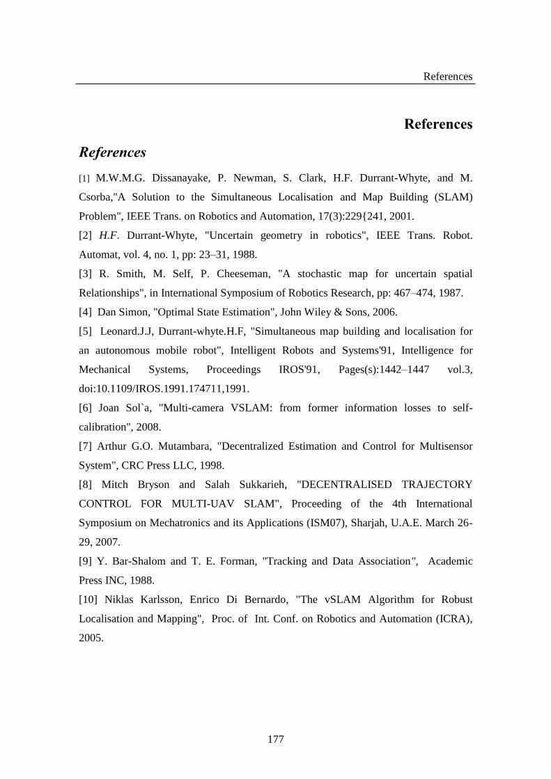
References
177
References
References
[1] M.W.M.G. Dissanayake, P. Newman, S. Clark, H.F. Durrant-Whyte, and M.
Csorba,"A Solution to the Simultaneous Localisation and Map Building (SLAM)
Problem", IEEE Trans. on Robotics and Automation, 17(3):229{241, 2001.
[2] H.F. Durrant-Whyte, "Uncertain geometry in robotics", IEEE Trans. Robot.
Automat, vol. 4, no. 1, pp: 23–31, 1988.
[3] R. Smith, M. Self, P. Cheeseman, "A stochastic map for uncertain spatial
Relationships", in International Symposium of Robotics Research, pp: 467–474, 1987.
[4] Dan Simon, "Optimal State Estimation", John Wiley & Sons, 2006.
[5] Leonard.J.J, Durrant-whyte.H.F, "Simultaneous map building and localisation for
an autonomous mobile robot", Intelligent Robots and Systems'91, Intelligence for
Mechanical Systems, Proceedings IROS'91, Pages(s):1442–1447 vol.3,
doi:10.1109/IROS.1991.174711,1991.
[6] Joan Sol`a, "Multi-camera VSLAM: from former information losses to self-
calibration", 2008.
[7] Arthur G.O. Mutambara, "Decentralized Estimation and Control for Multisensor
System", CRC Press LLC, 1998.
[8] Mitch Bryson and Salah Sukkarieh, "DECENTRALISED TRAJECTORY
CONTROL FOR MULTI-UAV SLAM", Proceeding of the 4th International
Symposium on Mechatronics and its Applications (ISM07), Sharjah, U.A.E. March 26-
29, 2007.
[9] Y. Bar-Shalom and T. E. Forman, "Tracking and Data Association", Academic
Press INC, 1988.
[10] Niklas Karlsson, Enrico Di Bernardo, "The vSLAM Algorithm for Robust
Localisation and Mapping", Proc. of Int. Conf. on Robotics and Automation (ICRA),
2005.

References
178
[11]. Luis Merino1, Fernando Caballero2, etc., "Multi-UAV Cooperative Perception
Techniques", Multiple Heterogeneous Unmanned Aerial Vehicles, Springer Tracts in
Advanced Robotics Volume 37, 2007, pp: 67-110.
[12] D. G. Lowe, "Distinctive image features from scale-invariant keypoints",
International Journal of Computer Vision, 60:91–110, 2004.
[13] Luis Merino, Fernando Caballero, J. R. Martínez-de Dios, etc., "A cooperative
perception system for multiple UAVs: Application to automatic detection of forest
fires", Field Robotics, Vol. 23, Iss 3-4, pp: 165-184, 2006.
[14] Mu Huaa, Tim Bailey, etc., "Decentralised Solutions to the Cooperative Multi-
Platform Navigation Problem", 2006.
[15] Julie Zhu, "A Peer-to-Peer Software Framework for Cooperative Robotic System",
Thesis for Master Degree, 2006.
[16] Mitch Bryson, Salah Sukkarieh, "Architectures for Cooperative Airborne
Simultaneous Localisation and Mapping", Journal of Intelligent and Robotics Systems,
Special Issue on Airborne SLAM, 2009.
[17] Bay H, Tuytelaars T,Van Gool L, "SURF: Speeded up robust features", In
Proceedings of the European Conference on Computer Vision, Graz, Austria, 2006.
[18] Lindeberg, T, "Feature detection with automatic scale selection", International
Journal of Computer Vision 30(2), pp: 79 – 116,1998.
[19] Mikolajczyk, K., Schmid, C, "Indexing based on scale invariant interest points",
ICCV, Volume 1, pp525 – 531, 2001.
[20] Luo Juan, "Comparison of SIFT, PCA-SIFT and SURF", Chonbuk National
University, Jeonju 561-756, South Korea, 2008.
[21] Eric Chu, Erin Hsu, Sandy Yu, "IMAGE-GUIDED TOURS: FAST-
APPROXIMATED SIFT WITH U-SURF FEATURES", Department of Electrical
Engineering Stanford University, 2008.
[22] Martin A. Fischler and Robert C. Bolles, "Random Sample Consensus: A
Paradigm for Model Fitting with Applications to Image Analysis and Automated
Cartography", Comm. of the ACM 24, pp: 381–395, 1981.
[23] Elan Dubrofsky, " Homography Estimation", MASTER Thesis, University of
Carleton, 2007.

References
179
[24] K.Kanatani, "Geometric information criterion for model selection",
IJCV,26(3):171-189,1998.
[25] KIM J, SUKKARIEH S, "Airborne simultaneous localisation and map
building[A]", In Proc. IEEE Int. Conf. Robotics and Automation[C]. 2003.406-411.
[26] Online, "SURVEILLANCE IMAGES",
http://www.imagefusion.org/images/octec/octec.html
[27] Online, "Fusion of EO and IR Video Streams", "http://iris.usc.edu/Vision-
Users /index.html.
[28] R. Smith, M. Self, P. Cheeseman, "A stochastic map for uncertain spatial
Relationships", International Symposium of Robotics Research, pp: 467–474, 1987.
[29] Andrew J. Davison, Ian Reid, Nicholas Molton and Olivier Stases, "MonoSLAM:
Real-Time Single Camera SLAM", IEEE Trans. PAMI 2007.
[30] Javier Civera, Andrew J. Davison and J. M. M. Montiel, "Inverse Depth to Depth
Conversion for Monocular SLAM" , ICRA 2007.
[31] Steven Holmes, Georg Klein and David W Murray, "A Square Root Unscented
Kalman Filter for visual monoSLAM", in Proc. of the IEEE International Conference on
Robotics and Automation, 2008.
[32] Niko Suinderhauf, Sven Lange and Peter Protzel, "Using the Unscented Kalman
Filter in Mono-SLAM with Inverse Depth Parametrisation for Autonomous Airship
Control", Proceedings of the 2007 IEEE International Workshop on Safety, Security and
Rescue Robotics, Rome, Italy, September 2007.
[33] Simon J. Julier Jeffrey K. Uhlmann, "A New Extension of the Kalman Filter to
Nonlinear systems", The University of Oxford, OX1 3PJ, UK
[34] R. Smith and P. Cheesman, "On the representation of spatial uncertainty", Int.
J.Robot. Res., vol. 5, no. 4, pp: 56–68, 1987.
[35]. S. Julier and J. K. Uhlmann, "A general method for approximating nonlinear
transformations of probability distributions", tech. rep., Robotics Research Group,
Department of Engineering Science, University of Oxford,1996.
[36] S. J. Julier, "The scaled unscented transformation", American Control Conference,
Proceedings of the 2002 (Volume:6 ), 2002.
[37] Houdai wen, Yinfu Liang, Chen Zhe, "Sigma Point H∞ Filtering Method for
References
180
Speaker Tracking", S IGNA L P R OC E SS INC, V 25 . No.3, Mar. 2009.
[38] Jun-hou Wang, Chun-lei Song, Xing-tai Yao, Jia-bin Chen,"Sigma Point H-infinity
Filter for Initial Alignment in Marine Strapdown Inertial Navigation System", 2nd
International Conference on Signal Processing Systems (ICSPS), 2010.
[39] Mitch Bryson and Salah Sukkarieh,"DECENTRALISED TRAJECTORY
CONTROL FOR MULTI-UAV SLAM", In 4th International Symposium on Mechanics
and its Application (ISMA), Shajah, UAE, 2007.
[40] A. Nemra and N. Aouf, "Experimental airborne NH∞ vision-based simultaneous
localisation and mapping in unknown environments" , Proceedings of the Institution of
Mechanical Engineers, Part G: Journal of Aerospace Engineering, Vol:224, no: 12,
2010.
[41] G. Sibley, G.S. Sukhatme, L. Matthies, "The iterated sigma point Kalman filter
with applications to long range stereo", in: Proceedings of the Second Robotics: Science
and Systems Conference, Philadelphia, PA, pp: 16–19, 2006.
[42] Thomas L. Marzetta, Gabriel H. Tucci and Steven H. Simon, "A Random Matrix–
Theoretic Approach to Handling Singular Covariance Estimates", IEEE
TRANSACTIONS ON INFORMATION THEORY, Volume 57, Issue 9, SEPT, 2011.
[43-1] M.W.M.G. Dissanayake, P. Newman, S. Clark, H. Durrant-Whyte and M.
Csorba, "A Solution to the Simultaneous Localisation and Map Building (SLAM)
Problem", IEEE Trans. on Robotics and Automation,vol:17, pp:229-241, 2001.
[44] H. Durrant-Whyte, "Uncertain geometry in robotics", IEEE Trans. Robot and
Automation, Vol4, pp:23-31, 1988.
[45] Andrew J. Davison and David W. Murray, Member, IEEE "Simultaneous
localisation and Map-Building Using Active Vision", IEEE transactions on pattern
analysis and machine intelligence, vol. 24, no. 7, July 2002.
[46] A. J. Davison, "Real-Time Simultaneous Localisation and Mapping with a Single
Camera", Proceedings of the 9th International Conference on Computer Vision,
pp:1403-1410, 2003.
[47] Jong-Hyuk Kim, Salah Sukkarieh: "Real-time implementation of airborne inertial-
SLAM", Robotics and Autonomous Systems 55(1): 62-71, 2007.

References
181
[48] Jungho Kim, Kuk-Jin Yoon, Jun-Sik Kim and Inso Kweon, "Visual SLAM by
Single-Camera Catadioptric Stereo SICE-ICASE", International Joint Conference, Oct.
18-21, Bexco, Busan, Korea, 2006.
[49] Arturo Gil, O´ scar Reinoso, etc., "Estimation of Visual Maps with a Robot
Network Equipped with Vision Sensors", In Proceedings of the European Conference
on Computer Vision, Graz, Austria, 2006.
[50] Lindeberg, T., Bretzner, L, "Real-time scale selection in hybrid multi-scale
representations", Scale-Space, 148–163,2003.
[51] Simon Julier (IDAK Industries), Jeffrey K. Uhlmann(University of Missour),
"General Decentralised Data Fusion with Covariance Intersection (CI)", In: Hall, D and
Llinas, J, (eds.), Handbook of Data Fusion, Chapter 12, pp: 12-1 to 12-25, CRC Press:
Boca Raton FL, USA, 2001.
[52] Seungkeun Kim, "Multi-sensor Fusion", Cranfield University of United Kingdom,
Lecture notes, 2010.
[53] T. Bailey, J. Nieto, M. Guivant, J. Stevens and E. Nebot, "Consistency of the EKF-
SLAM Algorithm", IEEE/RSJ International Conference on Intelligent Robots and
Systems, pp: 3562 – 3568, China, 2006.
[54] Brown, M., Lowe, D, "Invariant features from interest point groups", BMVC.
2002: 13th British Machine Vision Conference, Cardiff, 2002.
[55] Mikolajczyk, K., Schmid, C, "A performance evaluation of local descriptors",
PAMI 27 (2005), pp1615–1630, 2005.
[56] Dimitris Bouris , Antonis Nikitakis , etc., "Fast and Efficient FPGA-based Feature
Detection employing the SURF, algorithm", 18th IEEE Annual International
Symposium on Field-Programmable Custom Computing Machines, 2010.
[57] Zhou Kai, "Structure & Motion", Automation and Control Institute, ACIN, 2010.
[58] Marion Langer, Selim BenHimane, "An Interactive Vision-based 3D
Reconstruction Workflow for Industrial AR Applications", Metaio GmbH, 2010.
[59] Szeliski, Richard and Heung-Yeung Shum, "Creating Full View Panoramic Image
Mosaics and Environment Maps," Microsoft Research. SIGGRAPH 1997.
[60] Brown, M. and D. G. Lowe, "Recognising Panoramas", Department of Computer
Science, University of British Columbia, Vancouver, Canada. ICCV 2003.

References
182
[61] E Trucco,"Introductory techniques for 3-D computer vision", ISBN-13: 978-
0132611084 March 16, 1998.
[62] Abdelkrim Nemra,"Robust Airborne 3D Visual Simultaneous Localisation And
Map", PhD thesis, Cranfield University, UK, 2010.
[63] O. Faugeras, "What can be seen in three dimensions with an uncalibrated stereo
rig?", Computer Vision-ECCV’92, Springer Verlag, Lecture Notes in Computer Science,
588:563–578, 1992.
[64] Z. Zhang,"Determining the Epipolar Geometry and its Uncertainty: A Review",
The International Journal of Computer Vision, 27(2):161–195, March 1998. Also
Research Report No.2927, INRIA Sophia-Antipolis.
[65] M. Pilu, "Uncalibrated Stereo Correspondence by Singular Value Decomposition",
Technical Report HPL-97-96, Digital Media Department, HP Laboratories Bristol,
August 1997.
[66] Z. Zhang, R. Deriche, O. Faugeras, and Q.-T. Luong, "A Robust Technique for
Matching Two Uncalibrated Images Through the Recovery of the Unknown Epipolar
Geometry", Artificial Intelligence Journal, 78:87–119, 1995.
[67] Nira Dyn, David Levin, and Samuel Rippa, "Data Dependent Triangulations for
IPiecewise Linear Interpolation", IMA Journal of Numerical Analysis, Vol 10, pp137-
154, 1990.
[68] De Berg, Mark, Otfried Cheong, Marc van Kreveld, Mark Overmars,
"Computational Geometry: Algorithms and Applications", Springer-Verlag. ISBN 978-
3-540-77973-5, 2008.
[69] R. Hartley and A. Zisserman, "Multiple View Geomerty in Computer Vision",
Cambridge University Press, second edition, 2003.
[70] McConnell, Jeffrey J, "Computer Graphics: Theory into Practice", Jones &
Bartlett Learning, p 120. ISBN 0-7637-2250-2, 2006.
[71] Berger, Edmond Boyer et M.-O, "3D Surface Reconstruction Using Occluding
Contours", International Journal of Computer Vision, 22(3):219–233, 1997.
[72] Laurentini, Aldo, "How far 3D Shapes Can be Understood from 2D Silhouettes",
IEEE Transactions on Pattern Analysis and Machine Intelligence, 17(2):188–195, 1995.

References
183
[73] Xiaodong Li, Nabil Aouf, Abdelkrim Nemra, "3D Mapping based on VSLAM for
UAVs", IEEE Proceeding, Euro-Mediterranean Conference, MED2012, Barcelona,
Spain, 2012.
[74] Ruslana Mys, " Delaunay Triangulation (DT)", seminar, 2007
[75] Peter Su, Robert L. Scot Drysdale, "A Comparison of Sequential Delaunay
Triangulation Algorithms", Imperative Internet Technologies, 1986.
[76] David Capel, "Image Mosaicing and Super-resolution", Edition: illustrated.
Published by Springer ISBN 1852337710, 9781852337711, 2004.
[77] Robyn Owens, "Computer Vision", School of Informatics, University of
Edinburgh, Lecture Notes,
http://homepages.inf.ed.ac.uk/rbf/CVonline/LOCAL_COPIES/OWENS/LECT9/node2.
html, 1997.
[78] Arne Henrichsen,"3D Reconstruction and Camera Calibration from 2D Images",
thesis, University of Cape Town, 2000.
[79] P.R. Wolf, "Elements of Photogrammetry", McGraw-Hill, 2 edition, 1983.
[80] A. Watt, "3D Computer Graphics", Addison-Wesley, 2nd edition, 1995.
[81] S.B. Kang, "A survey of image-based rendering techniques", Technical Report
CRL 97/4, Digital Equipment Corp. Cambridge Research Lab, Aug 1997.
[82] Nader Salman, Mariette Yvinec, "Surface Reconstruction from Multi-View
Stereo", IEEE Trans. on Robotics and Automation, 17(3):pp229-241, 2001.
[83] Satya Prakash Mallick, "Feature Based Image Mosaicing", IEEE Trans. on
Robotics and Automation, 17(3), pp: 229-241, 2001.
[84] C.R. Rao, H. Toutenburg, A. Fieger, C. Heumann, T. Nittner and S. Scheid,
"Linear Models: Least Squares and Alternatives", Springer Series in Statistics,1999.
[85] Miguel Angel Garcia and Agusti Solanas, "3D Simultaneous Localisation and
Modelling from Stereo Vision", Proceedings of the 2004 IEEE, International
Conference on Robotics & Automation, New Orleans, LA ,April 2004.
[86] P. Newman, J. Leonard, J.D. Tardos and J. Neira, "Explore and Return:
Experimental Validation of Real-Time Concurrent Mapping and Localisation", IEEE
Int. Conf. on Robotics and Automation, pp: 1802 -1809, 2002.

References
184
[87] A.J. Davison and N. Kita, "3D Simultaneous Localisation and Map-Building
Using Active Vision for a Robot Moving on Undulated Terrain", IEEE Int. Conf. of
Computer Vision and Pattern Recognition. vol.1, pp: 384-391, 2002.
[88] Williams, S.B, Dissanayake, G. and Durrant-Whyte, H, "Towards multivehicle
simultaneous localisation and mapping", in Proc. International Conference on Robotics
and Automation (ICRA’02), 2002.
[89] Gang Xu, Zhengyou, Zhang, "Epipolar Geometry in Stereo Motion and Object
Recognition", Computational Imaging and Vision, Vol, 6, Springer,1996.
[90] Zhengyou, Zhang, "Camera Calibration", In G, editors: Medioni and S.B.Kang,
Emerging Topics in Computer Vision, Chapter 2, pp: 4-43. Prentice Hall, 2005.
[91] N. D. Molton, A. J. Davison, and I. D. Reid, "Locally planar patch features for
realtime structure from motion", In Proc. British Machine Vision Conference. BMVC,
Sep 2004.
[92] J.M.M.Montiel, J.Civera, and A.J.Davison," Unified Inverse Depth Parametrisation
for Monocular slam", In Proc Robotics: Science and Systems Conf., 2006.
[93] Andrea Vedaldi, Brian Fulkerson", VLFeat - An open and portable library of
computer vision", http://www.vlfeat.org/overview/sift.html.
[94] Jian Wu, Zhiming Cui, Victor S. Sheng, etc., "A Comparative Study of SIFT and
its Variants", MEASUREMENT SCIENCE REVIEW, Volume 13, No. 3, 2013.
[95] Baptiste Mazin, Julie Delon and Yann Gousseau, "Combining colour and geometry
for local image matching", MEASUREMENT SCIENCE REVIEW, 21st International
Conference on Pattern Recognition (ICPR 2012), November 11-15,Tsukuba, Japan,
2012.
[96] Tinne Tuytelaars and Krystian Mikolajczyk, "Local Invariant Feature Detectors: A
Survey", Foundations and Trends Computer Graphics and Vision, Vol. 3, No. 3, pp:
177–280, 2007.
[97] Koen E. A. van de Sande, Theo Gevers, and Cees G. M. Snoek. M, "Local
Evaluating Colour Descriptors for Object and Scene Recognition", IEEE Transactions
on Pattern Analysis and Machine Intelligence, Volume 32 (9), page 1582--1596, 2010.
[98] Luo Juan, Oubong Gwon, "A comparison of SIFT, PCA-SIFT and SURF",
Computer Graphics Lab, Chonbuk National University, South Korea, 2008.
References
185
[99] Max K. Agoston, " Computer Graphics and Geometric Modelling: Implementation
and Algorithms", London: Springer, ISBN 1-85233-818-0, 2005.
[100] A. Bosch, A. Zisserman, and X. Munoz, "Image classification using random
forests and ferns", In Proc. ICCV, 2007.
[101] A. Bosch, A. Zisserman, and X. Munoz, "Scene classification using a hybrid
generative/discriminative approach," IEEE Transactions on Pattern Analysis and
Machine Intelligence, vol. 30, no. 04, pp: 712–727, 2008.
[102] Morel, J.M, Yu, G, "ASIFT: A new framework for fully affine invariant image
comparison", SIAM Journal on Imaging Sciences, 2 (2), 438-469, 2009.
[103] P. Quelhas and J.-M. Odobez, "A Colour and Gradient Local Descriptor Fusion
Scheme For Object Recognition", In Proceedings of WIAMIS04, IDIAP, 2004.
[104] Jorge Artieda, Jose M. Sebastian, etc., "Visual 3-D SLAM from UAVs", Journal
of Intelligent & Robotic Systems, Volume 55, Numbers 4-5, pp: 299-321, 2009.
[105] Grisetti. G, Stachniss. C, Burgard. W, "Visual SLAM for Flying Vehicles", IEEE
Transactions on Robotics, Volume: 24, Issue: 5 pp: 1088 – 1093, 2008.
[106] Greer. J, Aouf Nabil, Richardson Mark A, etc., "Feature-based tracking
algorithms for imaging infrared anti-ship missiles", Proceedings of the SPIE Conference,
Volume 8187, pp: 81870T-81870T-15 (2011).
[107] Changhan Park, "SIFT-based object recognition for tracking in infrared imaging
system", 34th IEEE International Conference on Infrared, Millimeter, and Terahertz
Waves, 2009. IRMMW-THz, pp:1-2, 2009.
[108] Durrant-Whyte. H, Bailey.T, "Simultaneous Localisation and Mapping (SLAM):
Part I The Essential Algorithms", Robotics and Automation Magazine , June, 2006.
[109] Durrant-Whyte.H, Bailey.T, "Simultaneous Localisation and Mapping (SLAM):
Part II State of the Art", Robotics and Automation Magazine , September, 2006.
[110] Francesco Conte1,etc., "Cooperative Localisation and SLAM Based on the
Extended Information Filter", University degli Studi dell’Aquila, Italy.
[111] Josep AULINAS, Yvan PETILLOT, Joaquim SALVI and Xavier LLADÓ", The
SLAM Problem: A Survey ", Proceedings of the 11th International Conference of the
Catalan Association for Artificial Intelligence, pp363-371 IOS Press Amsterdam, 2008.

References
186
[112] Heon-Cheol Lee, Seung-Hwan Lee , Tae-Seok Lee , Doo-Jin Kim," A survey of
map merging techniques for cooperative-SLAM ", 2012 9th International Conference on
Ubiquitous Robots and Ambient Intelligence (URAI) , daejeon, Korea, 2012.
[113] J Fuentes-Pacheco, J.M. Rendon-Mancha, "Visual simultaneous localisation and
mapping: a survey", Online publishing, Springer Science+ Business Media Dordrecht,
2012.
[114] S. Thrun and Y. Liu, "Multi-robot SLAM with sparse extended information
filers", Proceedings of the 11th International Symposium of Robotics Research
(ISRR’03), Springer ,Sienna, Italy, 2003.
[115] S. Thrun, C. Martin, Y. Liu, D. Hähnel, R. Emery-Montemerlo, D. Chakrabarti,
and W. Burgard , "A real-time expectation maximisation algorithm for acquiring multi-
planar maps of indoor environments with mobile robots", IEEE Transactions on
Robotics and Automation, 20(3):433–442, 2004.
[116] S. Thrun, Y. Liu, D. Koller, A.Y. Ng, Z. Ghahramani and H. Durrant-Whyte,
"Simultaneous localisation and mapping with sparse extended information filters",
International Journal of Robotics Research, 23(7-8):693–716, 2004.
[117] M.R.Walter, R.M. Eustice and J.J. Leonard, "A provably consistent method for
imposing exact sparsity in feature-based SLAM information filters", Proceedings of the
12th International Symposium of Robotics Research (ISRR), pp: 241–234, 2007.
[118] M.R. Walter, R.M. Eustice and J.J. Leonard, " Exactly sparse extended
information filters for feature based SLAM", The International Journal of Robotics
Research, 26(4):335–359, 2007.
[119] B. Triggs, P. McLauchlan , R. Hartley and A. Fitzgibbon, "Bundle Adjustment -
A Modern Synthesis", ICCV 99: Proceedings of the International Workshop on Vision
Algorithms. Springer-Verlag. pp: 298–372. doi:10.1007/3-540-44480-7_21. ISBN 3-
540-67973-1, 1999.
[120] Douglas West, "Introduction to Graph Theory" , Prentice Hall, 2000.
[121] Gross and Yellen, "Graph Theory and Its Applications", CRC Press, 1998.
[122] D. Conte, P. Foggia, C. Sansone and M. Vento, "THIRTY YEARS OF GRAPH
MATCHING IN PATTERN RECOGNITION", International Journal of Pattern
References
187
Recognition and Artificial Intelligence, Vol. 18, No. 3, pp: 265-298, World Scientific
Publishing Company, 2004.
[123] Wendy Aguilar, Yann Frauel, Francisco Escolano,etc.,"A robust Graph
Transformation Matching for non-rigid registration", Image and Vision Computing 27
pp: 897–910, 2009.
[124] Mohammad Izadi and Parvaneh Saeedi ," Robust Weighted Graph Transformation
Matching for Rigid and Nonrigid Image Registration ", IEEE TRANSACTIONS ON
IMAGE PROCESSING, VOL. 21, NO. 10, OCTOBER 2012.
[125] Michael Warren, etc., "Large Scale Monocular Vision-only Mapping from a
Fixed-Wing sUAS " ,QUT, Australia, 2010.
[126] Xiaodong Li, Nabil Aouf, "SIFT/SURF Feature Analysis in Visible and Infrared
Imaging for UAVs " ,CIS2012, Ireland, 2012.
[127] Arturo Gil, Óscar Reinoso, Mónica Ballesta , David Úbeda, "Dealing with Data
Association in Visual SLAM " ,Computer Vision, Editor: Xiong Zhihui, ISBN 978-
953-7619-21-3, pp: 538, I-Tech, Vienna, Austria, November 2008.
[128] A Eshera, K S Fu, "An image understanding system using attributed
symbolic representation and inexact graph-matching ", IEEE PAMI, Volume 8, Issue 5
pp: 604-618,1986.
[129] Christmas W J, J Kittler and M Petrou, "Structural Matching in computer vision
using probabilistic relaxation", IEEE TRANSACTIONS ON PATTERN ANALYSIS
A N D MACHINE INTELLIGENCE, VOL. 17, NO. 8, pp749-764, AUGUST 1995.
[130] RC Wilson, ER Hancock, "Structural matching by discrete relaxation", IEEE,
Pattern Analysis and Machine Intelligence, IEEE Transactions on Volume 19 Issue 6,
pp: 634-648, 1997.
[131 PL Worthington, ER Hancock, "New Constraints on data-closeness and needle
map consistency for shape-from-shading", IEEE, Pattern Analysis and Machine
Intelligence , IEEE Transactions on Volume 21 Issue 12, pp: 1250-1267, 1999.
[132]Antonella Branca, Ettore Stella, Arcangelo Distante: "Feature matching
constrained by cross ratio invariance ", IEEE, Pattern Recognition, Volume 33 Issue 3,
pp: 465-481, 2000.

References
188
[133]Andrew DJ Cross, RC Wilson, ER Hancock, "Inexact graph matching using
genetic search ", Pattern Recognition, Volume 30 Issue 6, pp: 953-970, 1997.
[134] Lars Jacobsen and Kim S. Larsen, "Variants of (a,b)-Trees with Relaxed
Balance", International Journal of Foundations of Computer Science, 12(4): 455-478,
2001.
[135] Kim Shearer, Horst Bunke, Svetha Venkatesh ,"Video indexing and similarity
retrieval by largest common subgraph detection using decision trees", Pattern
Recognition, Volume 34, Issue 5, pp: 1075–1091, May 2001.
[136] Bruno T. Messmer, Horst Bunke, "A decision tree approach to graph and
subgraph isomorphism detection ", Pattern Recognition, 32 (12), 1998.
[137] Yang-Lyul Lee, Rae-Hong Park, " A surface-based approach to 3-D object
recognition using a mean field annealing neural network ", Pattern Recognition, 35
(2),pp299-316 , 2002.
[138] Denis Rivière, Jean-François Mangin, Dimitri Papadopoulos-Orfanos, Jean-Marc
Martinez, Vincent Frouin, Jean Régis, "Automatic recognition of cortical sulci of the
human brain using a congregation of neural networks ", Medical Image Analysis,
Volume 6, Issue 2, pp: 77–92, June 2002.
[139] Denis Rivière, et al, "Automatic recognition of cortical sulci using a congregation
of neural networks ", Medical Image Computing and Computer-Assisted Intervention–
MICCAI 2000. pp:40-49, Springer Berlin Heidelberg, 2000.
[140]Marco Carcassoni, Edwin R Hancock, "Correspondence matching with modal
clusters", Pattern Analysis and Machine Intelligence, IEEE Transaction on 25(12),
pp:1609-1615, 2003.
[141] Alberto Sanfeliu, Francesc Serratosa, René Alquézar, "Clustering of attributed
graphs and unsupervised synthesis of function-described graphs ", Pattern Recognition,
Proceedings, 15th International Conference on Vol:2, ISSN: 1051-4651, pp:1022 -
1025, 10.1109/ICPR.2000.906248, 2000.

References
189
[142] Szeliski, Richard, and Heung-Yeung Shum, "Creating full view panoramic image
mosaics and environment maps." Proceedings of the 24th annual conference on
Computer graphics and interactive techniques. ACM Press/Addison-Wesley Publishing
Co., 1997.
[143] Shum, H. & Szeliski, R, "Construction and refinement of panoramic mosaic with
global and local alignment", IEEE Int'l Conf. Computer Vision, ISBN: 81-7319-221-9
pp: 953-958, 10.1109/ICCV.1998.710831, 1998.
[144] Zoghlami, I. & Faugeras,O. & Deriche, R, "Using geometric corners to build a
2D mosaic from as set of images", Computer Vision and Pattern Recognition,
Proceedings, IEEE Computer Society Conference , ISSN : 1063-6919, pp: 420-425,
10.1109/CVPR.1997.609359, 1997.
[145] Capel, David, and Andrew Zisserman. "Automated mosaicing with super-
resolution zoom", Computer Vision and Pattern Recognition, Proceedings, 1998 IEEE
Computer Society Conference, ISSN: 1063-6919, pp:885-891, 10.1109/
CVPR.1998.698709, 1998.
[146] J.L Mundy, Andrew Zisserman, "Geometric Invariance in Computer
Vision", MIT Press, Cambridge, Massachusetts, USA, 1992.
[147] Lambert, J. H, " Photometria", sive de Mensura et Gradibus Luminis, Colourum
et Umbrae, Augsburg, 1760.
[148] Mach, E, " The Principles of Physical Optics: An Historical and Philosophical
Treatment ", , trans. J.S. Anderson and A.F.A. Young, Dutton, New York, 1926.
[149] F.L Pedrotti, L.M Pedrotti, "Introduction to Optics ", Prentice
Hall, ISBN 0135015456, 1993.
[150] Online, "Camera Calibration Toolbox for Matlab",
http://robots.stanford.edu/cs223b04/JeanYvesCalib/htmls/links.html.
[151] Tsai Roger Y, Online, " An Efficient and Accurate Camera Calibration Technique
for 3D Machine Vision", Proceedings of IEEE Conference on Computer Vision and
Pattern Recognition, Miami Beach, FL, pp: 364–374, 1986.
[152] O.D. Faugeras, G. Toscani, " The calibration problem for stereo", Proceedings of
the IEEE Computer Vision and Pattern Recognition, Florida, USA, pp: 15 –20, 1986.
References
190
[153] Luis Mej´ıas, Juan F. Correa, Ivan Mondrag, "COLIBRI: A vision-Guided UAV
for Surveillance and Visual Inspection", 2007 IEEE International Conference on
Robotics and Automation, Roma, Italy, 10-14 April 2007.
[154] S. Guha and S. Khuller, "Approximation algorithms for connected dominating
sets", Algorithmica 20(4), pp:374–387, April 1998.
[155] B Das, E Sivakumar and V Bhargavan, "Routing in ad hoc networks using a
virtual backbone", Proc. of the 6th Internat, Conf. on Computer Communications and
Networks (IC3N ’97), pp: 1–20, 1997.
[156]Wu J, Li H, "On calculating connected dominating set for efficient routing in ad
hoc wireless networks", Proceedings of the 3rd International Workshop on Discrete
Algorithms and Methods for Mobile Computing and Communications, ACM, pp:7–14,
1999.
[157] Stojmenovic I , Seddigh M, Zunic J, "Dominating sets and neighbor elimination-
based broadcasting algorithms in wireless networks", Parallel and Distributed Systems,
IEEE Transactions 13(1), pp:14 - 25 , 2002.
[158] J Alber, H L Bodlaender, H Fernau, T Kloks and R. Niedermeier, "Fixed
Parameter Algorithms for Dominating Set and Related Problems on Planar Graphs",
Algorithmica 33, pp: 461–493, DOI: 10.1007/s00453-001-0116-5, 2002.


