
University of New MexicoUNM Digital Repository
Physics & Astronomy ETDs Electronic Theses and Dissertations
Spring 5-10-2018
Vibrational Relaxation Theory for SystemsEmbedded in Microscopically Specified ReservoirsAnastasia Aemilia IeridesUniversity of New Mexico
Follow this and additional works at: https://digitalrepository.unm.edu/phyc_etds
Part of the Condensed Matter Physics Commons, Other Physics Commons, Quantum PhysicsCommons, and the Statistical, Nonlinear, and Soft Matter Physics Commons
This Dissertation is brought to you for free and open access by the Electronic Theses and Dissertations at UNM Digital Repository. It has beenaccepted for inclusion in Physics & Astronomy ETDs by an authorized administrator of UNM Digital Repository. For more information, please [email protected].
Recommended CitationIerides, Anastasia Aemilia. "Vibrational Relaxation Theory for Systems Embedded in Microscopically Specified Reservoirs." (2018).https://digitalrepository.unm.edu/phyc_etds/178

Anastasia Aemilia Ierides
Candidate
Physics and Astronomy
Department
This dissertation is approved, and it is acceptable in quality and form for publication:
Approved by the Dissertation Committee:
V. M. Kenkre, Chairperson
Arash Mafi
James Thomas
Anil Prinja

Vibrational Relaxation Theory for SystemsEmbedded in Microscopically Specified
Reservoirs
by
ANASTASIA AEMILIA IERIDES
B.S., Physics and Applied Mathematics, University of New Mexico,2011
M.S., Physics, University of New Mexico, 2014
DISSERTATION
Submitted in Partial Fulfillment of the
Requirements for the Degree of
Doctor of PhilosophyPhysics
The University of New Mexico
Albuquerque, New Mexico
May, 2018
c©2018, ANASTASIA AEMILIA IERIDES
iii

Dedication
To my sisters, Niki and Eleni, and my father, Loutsios,
for their support and encouragement of my endeavors, and for being my inspiration
to aspire to think differently and to afford compassion and understanding for
alternate perspectives or perceptions;
and to my mother, Maria, a mother’s love never dies.
“Now is the time to understand more, so that we may fear less.”
– Marie Curie
“I would rather have a mind opened by wonder than one closed by belief.”
– Gerry Spence
iv
Acknowledgments
The decision one makes as they enter the chaotic cobweb of career choices, whilstnot always permanent, can lead a student on a journey of discovery; discovery of theself, the world, and of the interconnectedness of the many aspects and subjects oflife. The path that hails itself before a student as they embark on such a journeycan lead to many triumphs and failures which would not be valued if it were not forthe obstacles which inspire originality, creativity, discipline, and dedication in one’swork.
Throughout my journey on such a path I have been fortunate enough to meetmany friends who have taken the active role of teaching, guiding, and fostering methrough the arduous tasks put before me. For me, the most esteemed of thesefriends, and the one who has inspired me most, is my adviser, Professor V. M.(Nitant) Kenkre. His artistry and the poetic form with which he presents, analyzes,and solves problems are only mirrored by the enthusiasm and care with which heteaches and counsels his students. For his support, tireless attention, and for themany great discussions and laughs had, I would like to extend my gratitude to him.
I am also grateful to Professor David Dunlap for his attentiveness in our groupmeetings and his guidance and help with various research projects. His tenacity inunderstanding the fundamentals of problems through physically meaningful conceptsand ideas is, in my opinion, unparalleled.
I would also like to extend my gratitude to Professor Susan Atlas for her keeninsights and valuable discussions as a fellow female scientist and mentor.
v

I would like to thank my friends and research group members without whosesupport and discussions this endeavor would almost be impossible: Satomi, Matt,and Tzu-Cheng. I would also like to thank my friends outside of the department whohave been patient and understanding of the demands of being a graduate student.
I am grateful to my committee members who have so graciously given up theirvaluable time to be a part of this process. I value their input and contributions toimproving the quality of my dissertation.
Lastly, I am immensely grateful to my sisters and father for their endless love,support, and encouragement during this journey, and to Mehmet, for brightening upeven the darkest days.
vi

Vibrational Relaxation Theory for SystemsEmbedded in Microscopically Specified
Reservoirs
by
ANASTASIA AEMILIA IERIDES
B.S., Physics and Applied Mathematics, University of New Mexico,
2011M.S., Physics, University of New Mexico, 2014
Ph.D., Physics, University of New Mexico, 2017
Abstract
This dissertation is a study of the theoretical framework of the practical as well as
fundamental problem of the process of relaxation to equilibrium of quantum mechan-
ical systems. The fundamental aspect is concerned with the simultaneous occurrence
of decoherence and population equilibration. The practical aspect deals with exper-
imental observations of vibrational relaxation of molecules embedded in liquids or
solids. The systems include, but are not limited to, the nondegenerate dimer and har-
monic oscillator, in one case weak and in the other strong, interaction with a thermal
bath. The time dependence of the energy and the temperature dependence of the
relaxation rate are the specific observables addressed in this dissertation. The anal-
ysis is based on the method of generalized master equations (GMEs). The memory
functions in the GME are derived from specified Hamiltonians with given, micro-
scopically formulated, interactions with specific reservoirs. The theory is developed
vii

with the help of projections and coarse-graining operator techniques with the as-
sumption of initial random phases. These memories are documented in the general
sense in terms of the time-correlation function of the interaction potential which is
the thermal average over bath states. For simple types of interaction potential, the
memories can be further written in terms of components contributed separately by
the system and bath. The bath contribution is an equilibrium thermal correlation
function. The memories and bath correlation functions are used to calculate the time
dependence of the energy of the system and the temperature dependence of the bath
spectral function or relaxation rate of the system, respectively. Predictions include
an interesting, perhaps unexpected, nonmonotonicity effect and oscillations of a re-
laxation memory with respect to temperature. The theory is briefly discussed in the
context of observations of the relaxation of specified molecular-bath interactions done
via pump-probe experiments. An interpolation formula for the time dependence of
the energy of the relaxing molecule is developed on the basis of the half-Markoffian
approximation and a result relating relaxation rates to hypergeometric functions is
presented. The thesis also contains a research contribution, unrelated to its primary
topic, concerning the macroscopic classical problem of the flow of granular materials.
viii

CONTENTS
Contents
Glossary xiii
1 Introduction 1
2 Background 6
2.1 Introduction . . . . . . . . . . . . . . . . . . . . . . . . . . . . . . . . 7
2.2 Experimental Observables . . . . . . . . . . . . . . . . . . . . . . . . 9
2.2.1 Relaxation of the Average Energy of a Molecule . . . . . . . . 11
2.2.2 Temperature Dependence of the Relaxation Rate . . . . . . . 13
2.3 Inverted Temperature Dependence in a
Reported Experiment . . . . . . . . . . . . . . . . . . . . . . . . . . . 14
2.4 The Master Equation of Montroll and Shuler . . . . . . . . . . . . . . 16
2.5 The Generalized Master Equations . . . . . . . . . . . . . . . . . . . 19
2.5.1 The GME via Projection . . . . . . . . . . . . . . . . . . . . . 20
2.5.2 Coarse-Graining . . . . . . . . . . . . . . . . . . . . . . . . . . 23
2.5.3 Transition Rates: Time Integrals of the Memories . . . . . . . 25
2.6 Generalization of the MSE: Kenkre and Chase . . . . . . . . . . . . . 27
2.7 Dressing or Polaronic Transformation . . . . . . . . . . . . . . . . . . 29
2.8 Concluding Remarks . . . . . . . . . . . . . . . . . . . . . . . . . . . 31
ix

CONTENTS
3 Calculation of Bath Correlations and Transition Rates for Explicitly
Given Microscopic Interactions 33
3.1 Introduction to Bath Correlations . . . . . . . . . . . . . . . . . . . . 33
3.2 Memories In Terms of Bath Correlations . . . . . . . . . . . . . . . . 35
3.2.1 Bath Spectral Function . . . . . . . . . . . . . . . . . . . . . . 36
3.2.2 Interaction Types . . . . . . . . . . . . . . . . . . . . . . . . . 38
3.3 Generalized Bath Correlation Functions . . . . . . . . . . . . . . . . . 41
3.3.1 Phonon Baths . . . . . . . . . . . . . . . . . . . . . . . . . . . 43
3.3.2 Optical Phonon Band . . . . . . . . . . . . . . . . . . . . . . . 45
3.3.3 Acoustic Phonon Band . . . . . . . . . . . . . . . . . . . . . . 46
3.4 Effects of Strong Coupling - Dressed Bath Correlation Functions . . . 50
3.4.1 Optical Phonon Band . . . . . . . . . . . . . . . . . . . . . . . 54
3.4.2 Acoustic Phonon Band . . . . . . . . . . . . . . . . . . . . . . 62
3.5 Effects of Weak Coupling - Bare Bath Correlation Functions . . . . . 65
3.5.1 Optical Phonon Band . . . . . . . . . . . . . . . . . . . . . . . 65
3.5.2 Acoustic Phonon Band . . . . . . . . . . . . . . . . . . . . . . 70
3.6 Concluding Remarks . . . . . . . . . . . . . . . . . . . . . . . . . . . 73
4 Application of the Theory to Vibrational Relaxation and Related
Topics 75
4.1 Introduction . . . . . . . . . . . . . . . . . . . . . . . . . . . . . . . . 75
x
CONTENTS
4.2 Equilibration of the Nondegenerate Dimer . . . . . . . . . . . . . . . 79
4.2.1 Multiphonon Temperature Effects on the Equilibration of a
Dimer . . . . . . . . . . . . . . . . . . . . . . . . . . . . . . . 83
4.2.2 Weak Coupling (Single-Phonon) Temperature Effects . . . . . 85
4.3 Charge in a 1-d Crystal Under a Strong Electric Field . . . . . . . . . 87
4.4 Energy of a Relaxing Molecule Modeled as a Harmonic Oscillator . . 94
4.4.1 Introduction of a Relaxation Memory and an Effective Rate . 100
4.4.2 The Half-Markoffian Approximation: Developing an Interpo-
lation Formula . . . . . . . . . . . . . . . . . . . . . . . . . . 102
4.5 Concluding Remarks . . . . . . . . . . . . . . . . . . . . . . . . . . . 104
5 Single-Mode Approximation and Connection to Hypergeometric
Functions 107
5.1 Proof of Strict Detailed Balance . . . . . . . . . . . . . . . . . . . . . 108
5.2 Approximate Detailed Balance After the Introduction of Disorder . . 113
5.3 Analytic Expression for a Special Case . . . . . . . . . . . . . . . . . 117
5.3.1 Hypergeometric Function 2F2 . . . . . . . . . . . . . . . . . . 118
5.3.2 Temperature Dependence of the Relaxation Rate: Investiga-
tions of the Effect of I` Propagators . . . . . . . . . . . . . . . 121
6 Concluding Remarks 124
Appendices 127
xi
CONTENTS
A Microscopic Connection to Phenomenological Memories 128
A.1 Single Mode of Vibration . . . . . . . . . . . . . . . . . . . . . . . . . 129
A.2 Lorentzian Spectral Function . . . . . . . . . . . . . . . . . . . . . . . 131
A.3 Gaussian Spectral Function . . . . . . . . . . . . . . . . . . . . . . . 132
B Investigation of the Classical Problem of Granular Materials 135
B.1 Introduction . . . . . . . . . . . . . . . . . . . . . . . . . . . . . . . . 136
B.2 Surface Profile Calculations In The Rotating Drum . . . . . . . . . . 138
B.2.1 Theory for Profile Prediction . . . . . . . . . . . . . . . . . . . 139
B.2.2 Present Analysis and Results . . . . . . . . . . . . . . . . . . 144
B.3 Comparison to Experiment . . . . . . . . . . . . . . . . . . . . . . . . 149
xii

Glossary
a Lattice constant
α Disorder in the crystal
B(t) Bath correlation function
β Thermodynamic beta which is the reciprocal of the product of the
product of the temperature T and Boltzmann constant kB
EM The energy of M -th state of the system
ε The Laplace domain variable
εm The energy of state m of the bath
FMN The relaxation rate from state N toM as defined by Fermi’s Golden
Rule or in terms of the memories or bath correlation functions
g(q) Dimensionless coupling constant (corresponding to phonons of wave-
vector q) or acceleration due to gravity (depending on the context)
H The complete Hamiltonian involved
HS(B) The component of the Hamiltonian contributed by the system S
(bath B)
xiii

Glossary
kB The Boltzmann constant
κ The relaxation rate of the system defined as κ = πY(0)
MSE Acronym for the Montroll-Shuler equation
ωmax The maximum or cutoff frequency as determined by the Debye
model and deformation potential approximation of the acoustic
phonon density of states
ω0 The peak or average frequency of the optical phonon band
Ω(MN) The characteristic system frequency defined by the energy difference
between system energy levels M and N
q The phonon mode, wavevector, or charge (depending on the context)
SE Acronym for the Schrödinger equation
σ The Gaussian width or dispersion of the optical phonon band
T Temperature
θ The scaled inverse temperature, θ = ~Ω/kBT , or angle between the
horizontal and arc (depending on the context)
V The system-bath interaction Hamiltonian
V(B,S),j The j-th contribution to the system-bath interaction contributed by
the bath (B) or system (S)
WMN(t) The memory function describing the transition from state N to M
Y(z) Bath spectral function
Z The bath partition function
xiv

Chapter 1
Introduction
The motivation for the work undertaken in this dissertation lies in the complexity
of the process of the irreversible relaxation to equilibrium of quantum systems, a
problem of both practical and fundamental importance. The practical aspect involves
the study of vibrational relaxation of molecules embedded in a liquid or solid in
chemical physics, wherein the time and temperature dependences of various system
relaxation properties are analyzed. The fundamental aspect involves the investigation
of the subtleties of the relaxation of a quantum system through processes including
decoherence and population equilibration after an external excitation of the system
has been turned off, necessitating a careful application of the principles of quantum
statistical mechanics.
Vibrational relaxation is the process by which a molecule, which has been ener-
getically excited by some external source, returns to its equilibrium state wherein
the occupation population of the energy states is Boltzmann-distributed. If the
system is embedded in a solid or liquid (thermal bath), the process consists of an
energy exchange and population equilibration from the internally excited vibrational
mode(s) via internal or external interactions to other modes in the system or “bath”
1

Chapter 1. Introduction
with which it is in contact. The process of vibrational relaxation is usually studied
through a specific type of time resolved spectroscopy known as “pump-probe” spec-
troscopy, wherein an initial pulse pumps the molecule to an excited state, while a
time-delayed pulse probes into the molecule, detecting the absorbance or transmit-
tance of the molecule over time as compared to the absorbance or transmittance of
the molecule in its equilibrium state. This type of spectroscopy allows for the analy-
sis of specific observables associated with the relaxation, the main two being the time
dependence of the average energy of the excited mode, E(t), and the temperature
dependence of the relaxation rate, κ = T−11 . Typically it is observed that the time
evolution of the average energy is of exponential form, decaying over time, while the
relaxation rate increases with temperature with a dependence on the phonon occu-
pation factor. However, some experimental results have shown that this “intuitive”
temperature dependence is not necessarily always true. These results provide one of
the motivations for the study of vibrational relaxation.
Understanding the relaxation behavior of a quantum system for all time, as a
result of interactions with its environment, is of fundamental importance. In partic-
ular, understanding how the simultaneous processes of decoherence and population
equilibration occur is essential. Take, for instance, an isolated quantum system with
Hamiltonian HS placed in one of its eigenstates. If left alone, it will remain in that
eigenstate, only the phase changing in time. At longer times, if the system is not
isolated but in interaction with a reservoir, the postulate of equilibrium statistical
mechanics states that the system is taken back to equilibrium, wherein its density
matrix will be diagonal in the representation of HS eigenstates, the diagonal terms
having corresponding Boltzmann weights. Understanding how the two processes oc-
cur simultaneously, that is, the phase relaxation through decoherence, wherein the
off-diagonal elements of the density matrix tend to zero in the representation of
the eigenstates of the Hamiltonian, and population relaxation, wherein the occupa-
tion probabilities are Boltzmann-weighted, requires the introduction of a model of a
2

Chapter 1. Introduction
system in interaction with a thermal reservoir or bath.
With the above in mind, the Schrödinger equation (SE) which is used to study
the behavior of a system, either in isolation or in interaction with its environment or
some potential, is applied in an effort to find the system’s spectrum of energies and
the system’s eigenstates or wavefunctions through the relation
HS|N〉 = EN |N〉.
In the case of a system in interaction with some external potential or environment,
call it a reservoir or bath, the full Hamiltonian is a sum of terms of the system, bath,
and interaction components
H = HS +HB + V .
Since there are very few systems for which the SE is exactly solvable, and particularly
for situations in which an interaction with some external potential exists, the SE
problem becomes extremely difficult to solve exactly due to the complex nature of
the quantum properties and processes involved. In order to simplify the method for
solving the SE for more complicated problems, theoreticians involved in chemical
and/or quantum physics and quantum chemistry, have developed many intricate
and sophisticated methods to calculate the wave functions and energy levels of the
specified problems. Perturbation theory is one such method wherein the Hamiltonian
is taken to be one that is slightly different from one whose SE solution is known, i.e.,
whose energies and wavefunctions are known, with the slight difference being treated
as a weak perturbation.
The weak perturbative treatment is usually viewed as a shortcoming in quantum
mechanics. However, when discussing the problem of relaxation to equilibrium from a
statistical mechanics standpoint, the weakness of the coupling between the bath and
the system described in the term V is actually a requirement. It arises from the need
that the bath should leave no signature of itself on the system density matrix at long
3

Chapter 1. Introduction
times, except for the value of the bath temperature on the Boltzmann population.
Yet the coupling must be strong enough to guide the system to its equilibrium state
through population and phase relaxation.
This dissertation aims to answer questions which arise from experimentally ob-
served time- and temperature-dependent quantities. An overview is given of the
experimental observations and theoretical framework for studying the vibrational
relaxation/relaxation to equilibrium of molecules in interaction with thermally in-
ert baths, followed by descriptions of new developments in, and applications of, the
theory. In Chapter 2, experimental techniques used in the study of vibrational re-
laxation are introduced briefly, followed by spectroscopic observations along with a
discussion of some important observables of interest. A brief introduction is also
made to the problem of irreversible relaxation to equilibrium and to the theoretical
tools used in the present study. Within the description, some basic quantum me-
chanical methods, the projection operator technique, and polaronic transformations
of interest are introduced and discussed.
In Chapter 3, microscopically formulated interactions between a nondegenerate
system and bath are discussed through the calculation of the corresponding separable
interaction correlation functions from microscopically specified Hamiltonians. The
focus, in part, is on the case in which a strong system-bath interaction necessitates
a dressing transformation which is discussed in the later part of Chapter 2. This is
followed by a brief discussion of the bath correlation functions in the weak interac-
tion case wherein the Hamiltonian is directly amenable to a perturbative treatment.
In Chapter 4, the theory is used to study the relaxation behavior of three quantum
systems in both interaction strength regimes through the time-evolution of their cor-
responding observables. The temperature effect on that relaxation behavior, which
shows a noteworthy effect in the relaxation behavior for all three systems, is also
discussed. The observables (and the three systems) are the occupation probability
4

Chapter 1. Introduction
difference for the nondegenerate dimer, the velocity (as it approaches a steady-state
value) of a charged particle moving in a crystal under electric fields strong enough
to produce a Stark ladder, and the energy of a relaxing molecule represented by a
harmonic oscillator. Surprising effects are uncovered in the relaxation of strongly in-
teracting systems. Special theoretical techniques are developed to investigate these
effects. In Chapter 5, the analysis of the strong interaction with a single mode of vi-
bration is made with connections to a specific case of the generalized hypergeometric
functions depicting unique behavior with the variation of microscopically specified
parameters. In Chapter 6, a summary is provided. In Appendix A, comparisons of
three cases of bath interactions, introduced earlier phenomenologically, are compared
to microscopically specified counterparts in this dissertation. Finally, some research
unrelated to other Chapters is presented as Appendix B. It describes the classical
problem of the flow of granular material inside a rotating drum.
5

Chapter 2
Background
In this Chapter, essential features of the background necessary to understand the
new results obtained in this dissertation are described, including a discussion of
experiments on vibrational relaxation and the introduction of the theoretical tools
employed, along with a review of some more recent contributions and generalizations
to the theory. In Section 2.1, a brief mention is made of the experimental techniques
used in obtaining data pertaining to vibrational relaxation; a more in-depth discus-
sion of experimental methods and more can be found in texts such as refs. [1,2] and
reviews such as refs. [3, 4]. In Section 2.2, an introduction is given of two experi-
mental observables, the time-dependent energy E(t) and the temperature-dependent
relaxation rate T−11 , in terms of the methods used to obtain them. Following that,
in Section 2.3 the experimental results reported in 1994 by Fayer and collaborators
are discussed which detail the temperature-dependence of the relaxation rate for two
molecules embedded in solvents, wherein an “inverted ” temperature-dependence was
observed [5].
Section 2.4 briefly introduces the reader to Master Equations (MEs) and the
specific master equation used to describe the vibrational relaxation of a relaxing
6

Chapter 2. Background
molecule represented as a harmonic oscillator by Montroll and Shuler in ref. [6].
In Section 2.5, discussed are the generalized master equations (GMEs), the tools
in nonequilibrium statistical mechanics used to bridge the gap between microscopic
(complex, many-body, with a large number of variables) and macroscopic (simple,
typically one-body) system dynamics. The projection operator technique of Zwanzig
through which GMEs may be obtained is outlined, with a summary of the coarse-
graining extension made by Kenkre for practical [7] and fundamental [8] purposes.
In Section 2.6, the recent generalization of the Montroll-Shuler equation is reviewed,
along with the generalization of equations describing the time evolution of observables
relevant in this study. Then in Section 2.7, an overview is given of the transformation
made when a system is in strong interaction with its environment in order to bring
the associated Hamiltonian into a representation in which the interaction is made
weak. In Section 2.8, concluding remarks are presented.
2.1 Introduction
Spectroscopy, in its simplest and encompassing description, is the study of the inter-
action of light with matter. The simplest example, for instance, is the study of how,
given specified environmental conditions, either a beam of light or molecular struc-
ture may be affected as light passes through the medium in question, the light being
refracted (absorbed, emitted, etc.) by the molecule or molecular aggregate surface.
The scope of spectroscopy spans several subcategories including, but not limited
to, absorption and emission, electronic, resonance, rotational, and vibrational spec-
troscopy. Of interest in this study is the time- and temperature-dependent behavior
of molecules undergoing vibrational relaxation through their interaction with micro-
scopically specified environments. In theory, the statistical mechanics involved in the
irreversible relaxation to equilibrium is governed by some interaction with a thermal
7

Chapter 2. Background
bath. Given that the interaction is weak enough, if it is true that the bath leaves no
signature on the system other than its temperature, the behavior of the relaxation
can be attributed entirely to the molecule. In experiment, vibrational spectroscopy
is the study of the relaxation of excitations in molecules (or crystal aggregates) after
some external influence has been turned off, usually the external source being a high
intensity laser or impact with some external agency.
The relaxation process involves the dissipation of the average energy and energy
level occupation of the molecule through dephasing and population equilibration
processes, including damping of the nuclear motion as energy is transferred among
chemical bonds [4,9]. In gases, relaxation processes occur through collisions between
molecules, while such processes in solids (which can be described as frozen out liq-
uids) manifest through interactions of (de-)localized charge-carriers (or excitations)
with lattice vibrations described by quasi-particles known as phonons [3,9,10]. In liq-
uids, however, it has been argued (and experimentally observed) that the vibrational
relaxation differs quite considerably from the aforementioned case. The anharmonic-
ity of the corresponding liquid phonons and the liquid density of states are thought
to play a vital role in the temperature dependences and time scales of the relax-
ation behavior of molecules [3,5]. These effects limit the types of processes that can
take place as well as the allowed relaxation pathways through which energy may be
transferred [4, 11,12].
In refs. [3,4], concise and summarizing reviews of theories, the types of computa-
tional simulations used, and experimental results are given for vibrational relaxation
in liquids. In particular, in ref. [3], Oxtoby gives an extensive discussion of obtain-
ing spectral lineshapes of molecules (two-level and multi-level systems) dissolved in
solvents along with a summary of hypothesized explanations of the potential mech-
anisms by which relaxation may occur as described by many in the literature; for
more in-depth reading, the reader is referred to ref. [3]. Since Oxtoby’s review, many
8
Chapter 2. Background
experiments have been conducted, attempting to validate or invalidate the various
theories introduced in order to understand the process of vibrational relaxation in
liquids and the temperature effects on the relaxation behavior.
In a more recent review discussing advancements in experimental techniques as
well as theoretical treatments of such processes, Owrutsky et. al. give a list of
experimentally obtained vibrational relaxation times for various small molecules (di-
atomics and triatomics) in corresponding solutions and liquids [4]. The importance
of studying small molecules is emphasized due to their simplicity in terms of theoret-
ical modeling and the mechanisms involved in their relaxation when in interaction
with a surrounding solvent or liquid. It is argued that the simple mode coupling
between smaller molecules and the liquid limits the number of pathways through
which energy can flow, as the energy of the excited molecule is dissipated directly by
such coupling. This aligns with theoretical arguments in which the simplest case of
analyzing the relaxation rates of such molecules will depend on the direct coupling
of the molecule’s vibrational mode(s) to the modes of the liquid.
2.2 Experimental Observables
Various techniques have been developed in the past few decades in order to study the
vibrational relaxation dynamics of molecules in solvents. The most popular method
is that of transient vibrational spectroscopy or pump-probe (IR or Raman) spec-
troscopy in which a pump pulse, tuned to the frequency of the vibrational transition
being investigated, is sent to the material, creating a nonequilibrium distribution of
the vibrational states, while the transient decay back to equilibrium is monitored by
a time-delayed and weaker probe pulse tuned to the same frequency [1, 2, 4, 11].
As mentioned above, there are two observables that are of interest in vibrational
relaxation studies, one being the decay time (or its reciprocal, the relaxation rate)
9

Chapter 2. Background
ln T
/T0
IR pump
probe
t < 0 t = 0
Vn
t = t1
Time Delay, 𝜏D
t = tn
Vf
Vi
IR pump
Vf
Vi
Solute
Intramolecular Solute Vibrations
Intermolecular Solvent Vibrations
Solvent Phonon ModesSolvent
Figure 2.1: Schematic depicting a typical pump and probe technique applied for thestudy of the vibrational relaxation within the ground electronic state [1, 2, 5, 11, 12].Visible are the occupation dynamics of the vibrational levels Vn as the molecule isprobed at intermediate delay times tn as the data is obtained during experiment. Theenergy level diagram (bottom) shows the various energy dissipation pathways thatthe nonradiative relaxation process might take, starting from the initially excitedvibrational level Vf .
associated with the approach to equilibrium of the average energy, and usually de-
noted by T1 (also known as longitudinal time), and the other the dephasing time,
denoted by T2 (also known as transverse time), which is usually much shorter than
the energy relaxation time, and is associated with decoherence. Both of these vari-
ables are known to be affected not only by the solvent in which the molecules are
placed and the strength of the coupling between the molecular aggregate and solvent
modes, but also the temperature at which the measurements are made.
10

Chapter 2. Background
2.2.1 Relaxation of the Average Energy of a Molecule
If a molecule is excited vibrationally in some manner such as by a laser in a pump-
probe arrangement in the laboratory or through impact with an external agency, it
would typically undergo relaxation resulting in the dissipation of the energy put into
the molecule by the excitation process through vibrational energy transfer. Such a
relaxation process can often occur on a timescale of a few hundred picoseconds (ps) or
less [3,4,9]. When discussing energy or population relaxation the variable of interest
is the relaxation time involved, denoted in the literature as T1, as the lifetime of
population equilibration is longer than that of the phase relaxation time, denoted by
T2, which describes the loss of phase coherence. The energy or population relaxation
rate is governed by the Bethe-Teller [13] equation
dE(t)
dt= − 1
T1
[E(t)− Eth] , (2.1)
which models the relaxation of a molecule represented by an oscillator through the
associated time-dependent observable, the average non-equilibrium energy E(t) as
it approaches its equilibrium value Eth. The assumption of this model is that the
interactions are of Landau-Teller type, wherein the coupling between the solvent and
solute modes is considered linear in the molecular displacement [4, 6].
In the typical experiment in which the energy relaxation time is obtained, the
changes in the pumped or excited optical quantities of the sample (such as ab-
sorbance, transmission, or reflectivity) are monitored over time and compared to
the corresponding equilibrium state values of the sample. These changes are mea-
sured through the time-delayed probe pulse and analyzed as functions of the delay
time τD between the pump and each consecutive probe pulse [1,2,9], yielding a direct
measurement of the relaxation rate T−11 . A gauge for the relaxation time may be
obtained, for instance, through the simple expression relating the log of the ratios
of the non-equilibrium and equilibrium transmissions, T/T0, and the delay time τD
11

Chapter 2. Background
Figure 2.2: Shown are representative decay time T1 data for the CO(ν = 1) stretchingvibration mode of metal carbonyl complexes in several solvents at room temperature(295 K). The data were taken from Fig. 2 of ref. [14] and Figs. 3 and 4 of ref.[15] and replotted to show how the relaxation time may be extrapolated from trans-mission data using Eq. (2.2). The data represent solute/solvent combintations asfollows: solid circles (•) are for W(CO)6/CCl4 with T1 = 1030± 70 ps; squares withcrosses () are for Cr(CO)6/n-Hexane with T1 = 144 ± 4 ps; triangles (N) are forIr(CO)Cl(TPP)2/CHCl3 with T1 = 58±3 ps; stars (F) are for Rh2(CO)4Cl2/CHCl3with T1 = 690 ps; and diamonds (♦) are for Co4(CO)12/CHCl3 with T1 = 390 ps.
[1,9]. The quantity describing such a relation is the signal detected S(t) as a function
of delay time τD,
S(τD) = ln
(T
T0
)= S(t0)e−τD/T1 , (2.2)
where t0 is the initial time at which the system is probed [9,14]. Eq. (2.2) is derived
through the use of rate equations which model the time evolution of the occupation
populations of the vibrational states and is detailed in refs. [1, 9]. The second
equality in Eq. (2.2) is most appropriate for the relaxation of lower vibrational modes,
12
Chapter 2. Background
where the anharmonicity of molecules does not affect the relaxation process, and the
exponential decay is considered to be a quite reasonable fit to the signal. Indeed,
most Raman and IR studies made involve the relaxation of high frequency vibrational
modes > 1800 cm−1, with the relaxation occurring in the ground electronic state,
between various vibrational levels, such as transitions between the ν = 1 and ν = 0
vibrational levels [4]. Fig. 2.2 shows examples of experimentally obtained relaxation
times using the relation in Eq. (2.2). Replotted there are data taken from refs.
[5, 9, 14] to show how the corresponding vibrational relaxation times (T1) may be
obtained from exponential fits to the experimental values for various solute/solvent
combinations undergoing population relaxation of the lower vibrational modes such
as the ν = 1 mode of CO in metal carbonyl complexes embedded in liquid solvents
[5, 14–16].
2.2.2 Temperature Dependence of the Relaxation Rate
The vibrational relaxation rate of a molecule or molecular aggregate dissolved (or
embedded) in a specified solvent or liquid depends on the temperature of whatever
(reservoir, bath, etc.) is in contact or interacting with it. It has been shown in exper-
iments that the relaxation rate can have various temperature dependences depending
on the system, the solvent, and interactions involved in the relaxation process [5].
In processes such as chemical reactions, an Arrhenius temperature dependence
of the relaxation rate is intuitively expected, the rate increasing with an increase in
the temperature of the bath. The qualitative reason for this expectation is that the
pathways for interaction are thought to increase in number along with the motion of
entities such as atoms or molecules constituting the bath. The increase introduces
a vibrational complexity in the system. Intuitively, when harmonic oscillators are
involved in the reservoir, one would expect the relaxation rate to be proportional
to the number of quantized excitations of the oscillator, more appropriately to the
13

Chapter 2. Background
factor, n(Ω) or n(Ω) + 1, where n(Ω) =(eβ~Ω − 1
)−1 depending on the energetic
direction. Here Ω is the frequency of the oscillator. The presence of the additive
1 is representative of spontaneous emission [6, 17]. The factor n(Ω) + 1 essentially
becomes proportional to the temperature for high values of T (i.e., T ~Ω/kB).
However, the situation is generally much more complex. Depending on the values
of the various parameters of the molecule and the solvent, the assumption that the
temperature dependence of the rate is solely described by the factor n(Ω) + 1 may
be invalid. It has been shown in experiment [14] that an increase in the solvent
vibrational complexity, results in a decrease in the vibrational lifetime of the excited
mode under study for various polyatomic molecules. As a result, it appears that
the intuitive expectation of the relationship of the rates to temperature may not
necessarily be so straightforward.
2.3 Inverted Temperature Dependence in a
Reported Experiment
In 1994, Fayer and collaborators began the experimental investigation of this and
related issues on the basis of picosecond pump-probe observations of a variety of
large molecules dissolved in several different solvents which constituted the bath. In
particular, they reported [5] the temperature dependence of the relaxation lifetime
of the T1u stretching mode of CO in two metal carbonyls, chromium hexacarbonyl,
Cr(CO)6, and tungsten hexacarbonyl, W(CO)6, in two solvents, carbon tetrachloride,
CCl4, and chloroform, CHCl3, in the temperature range of 220 K to 340 K. The
remarkable finding was that, while the relaxation rate followed “normal” behavior
(an increase of the relaxation rate with an increase in temperature), in three of the
four solvent-molecule combinations, it decreased with an increase in temperature for
14

Chapter 2. Background
Figure 2.3: Shown are the reciprocal of the vibrational relaxation time, T1, exper-imentally obtained through pump-probe experiments of the two metal carbonyls,Cr(CO)6 (left) and W(CO)6 (right), in chloroform, CHCl3. The data were takenfrom Fig. 5 of ref. [5] and replotted showing the temperature dependence of thecorresponding vibrational relaxation rates (κ = T−1
1 ).
W(CO)6 dissolved in CHCl3. This departure from what is typically expected has
been sometimes thought of as counter-intuitive. There seems to be no simple way to
connect the departure to properties of either solvent or either molecule.
Fayer and collaborators ascribed the breakdown of the simple assumption of the
n(Ω) + 1 temperature dependence to the temperature dependence of the liquid den-
sity of states of the solvent. This may well be the actual source of the observed
behavior with similar arguments of the solvent properties’ effects on the behavior of
the relaxation process being found in refs. [3, 4, 9, 14]. On the other hand, we be-
lieve that simpler considerations based on well-known polaron concepts can, perhaps
more naturally, lead to the “counter-intuitive” temperature dependence. Although
a discussion of this inverted trend of the temperature dependence of the relaxation
rates has not been seen in the literature in the last two decades or so since the in-
15

Chapter 2. Background
teresting observation made in refs. [5, 12], we have found it appropriate to consider
it an important question and address it in Chapters 3 and 4 in terms of a theory we
have constructed.
Our work in Chapters 3 and 4 investigates polaronic processes arising from strong
coupling to phonons and show how such processes can provide an alternative expla-
nation of the peculiar “inverted” temperature dependence of the relaxation rate of
W(CO)6 dissolved in CHCl3. The source suggested here, is similar to that shown [18]
to give rise to the observed T -dependence of the mobility of photo-injected holes in
aromatic hydrocarbon crystals [19]. It stems from oppositely trending effects of vir-
tual phonons and appears to be at least as natural and physical as the T -dependence
of the liquid phonon density of states of solvents. In the next few Sections, the
theoretical framework underlying the basis of such theory is discussed.
2.4 The Master Equation of Montroll and Shuler
An endeavor in nonequilibrium statistical mechanics is to close the gap that exists
in describing the dynamics of a system between the macroscopic and microscopic
worlds. In statistical mechanics, when the dynamics of a many-body system at any
given time are studied, the system is described as being in a probabilistic mixture of
states, wherein the time-evolution of the occupation probability PM(t) of each state
M is governed by a set of time differential equations known as master equations
dPM(t)
dt=∑N
[FMNPN(t)− FNMPM(t)] . (2.3)
Here the FMN ’s are the time-independent transition rate constants between the sys-
tem states N and M , the evolution among states being determined by a transition
rate or interaction matrix, F, composed of the rate constants.
In the 1950’s the theoretical groundwork for understanding vibrational relaxation
16

Chapter 2. Background
was laid out through the use of a particular Master equation developed by Kurt E.
Shuler, a chemical physicist. He began work on studying the dynamics of the relax-
ation to equilibrium of an externally induced non-equilibrium distribution of a system
of harmonic oscillators, first in collaboration with Robert J. Rubin, a mathemati-
cian and physicist, and later with Elliott W. Montroll, a chemist and mathematician
[6, 20]. The system analyzed to represent the relaxing molecule was a harmonic os-
cillator in interaction with a thermal bath. The bath was taken to remain at its
equilibrium temperature, T , throughout any energy exchange between the system
and bath molecules.
The time-independent transition rate constants FMN describing transitions be-
tween states N and M in Eq. (2.3), were derived through the use of Landau-Teller
type transition probabilities [21] wherein the perturbations inducing the transitions
between states were taken to be linear in the displacement of the harmonic oscillator
and sufficiently small, such that only nearest-neighbor transitions are possible. The
resulting set of differential difference equations
1
κ
dPMdt
= (M + 1)PM+1 + e−β~ΩMPM−1 −[M + e−β~Ω(M + 1)
]PM ,
for M = 0, 1, 2, · · · , (2.4)
now known as the Montroll-Shuler equation (MSE) [6, 20], describes the time evo-
lution of the occupation probability of a given vibrational level, M . In Eq. (2.4),
β = 1/kBT with kB being the Boltzmann constant and T the temperature, and
~Ω is the oscillator energy, with ~ being the Planck constant and Ω the oscillator
frequency.
17
Chapter 2. Background
Through the use of the technique of factorial moments,
fN(t) =∞∑
M=0
M(M − 1) · · · (M −N + 1)PM(t) =∞∑
M=0
M !
(M −N)!PM(t),
for N = 1, 2, · · · ,
f0(t) =∞∑
M=0
PM(t) = 1, (2.5)
Montroll and Shuler were able to calculate the energy of a vibrationally relaxing
molecule represented by a harmonic oscillator as
E(t) = ~Ω∞∑
M=0
(M +
1
2
)PM(t) = ~Ω
[f1(t) +
1
2
](2.6)
and were able to re-obtain the Bethe-Teller relation [13] for the average energy,
dE(t)
dt= −κ
(1− e−β~Ω
)[E(t)− Eth] (2.7)
where
Eth =~Ω
2coth
(β~Ω
2
)(2.8)
is the thermal or steady-state value of the energy of the oscillator. It was noted by
Montoll and Shuler that the average energy is independent of the initial distribution
of the oscillators at all times and that it only depends on the initial energy of the
system [22,23].
Throughout their series of papers, Shuler, Montroll, et. al. [6, 20, 22, 24–28],
studied the effects of the initial non-equilibrium distribution on the dynamics of the
approach to equlibrium, focusing on the time-evolution of various distributions of the
system of harmonic oscillators. These studies included the use of various conjectured
transition probabilities incorporating inter- and intra-electronic-level vibrational and
vibration-rotation interactions [20,24,25,28–30], and the anharmonicity of the oscil-
lator through the Morse oscillator model [26, 27]. The reached consensus was that,
18
Chapter 2. Background
in addition to the need for more accurate experimental data and an extension of the
theoretical tools involved, knowledge or precise prediction of the transition types con-
sidered, the microscopic parameters involved in the relaxation process (such as the
characteristic vibrational temperature ~Ω/kB and temperature T ), and relaxation
mechanisms involved is necessary for an accurate understanding of the relaxation
behavior of the system being investigated.
2.5 The Generalized Master Equations
While the ME is particularly useful in describing the long-time evolution of a system
to equilibrium, furnishing the user with the long-time and steady-state behavior of
variables under question, it fails to account for the short-time response of a system to
its surroundings before the decoherence of quantum phases has occured. Beginning
in the late 1950’s and extending into the 1960’s, many contributions were made in
the generalization of MEs in order to connect short-time and long-time evolutionary
behavior [31–39]. A significant contribution made by Zwanzig in ref. [38], shows con-
nections between the many generalizations of MEs, deriving the generalized master
equation (GME) from the Schrödinger equation as
dPM(t)
dt=
∫ t
0
ds∑N
[WMN(t− s)PN(s)−WNM(t− s)PM(s)] , (2.9)
where PM(t) is the occupation probability of state M , and the W(t) functions are
the memory possessing transition functions describing the behavior and evolution of
a system to equilibrium for all time through transitions between states [8]. Here the
subscript MN of the memory WMN(t) denotes the transition from N to M . The
memory functions inherent in the GME have the advantage of containing memory
of the behavior of the system for all time, enabling the GME to produce results for
short-time events as well as long-time behavior through the incorporation of the time
integral over the memory functions between states.
19

Chapter 2. Background
It is easy to see how the ME in Eq. (2.3) can be obtained from the GME in
Eq. (2.9), as the ME is the Markoffian limit of the GME, that is, it is the case for
which the memory functions are approximated as delta functions in time with inte-
grals equal to the transition rate between states, WMN(t) = FMNδ(t). However, Eq.
(2.9) becomes particularly useful in understanding how the process of decoherence
occurs at the initial stages of vibrational relaxation while undergoing simultaneous
population equilibration, the fundamental problem alluded to earlier in Chapter 1.
In the following Subsections, a derivation of the GME is outlined via projection op-
erators with coarse-graining included through which the evolution of the occupation
probability of level M can be derived in terms of the interaction from microscopic
descriptions. The memories are derived in terms of interaction correlation functions,
followed by derivations of the transition rates as time integrals of the memory func-
tions.
2.5.1 The GME via Projection
One way through which the GME may be derived is through the use of the projection
operator technique introduced in the literature by Zwanzig [33]. The projection
operator technique has as its basis the Von Neumann equation,
i~∂ρ
∂t= [H , ρ] = Lρ, (2.10)
where L is the Liouville operator, which may be broken up into its components, i.e.,
L = L0 + Lstimulus, (2.11)
where the stimulus component Lstimulus corresponds to the perturbation or external
influences on the system and L0 corresponds to the unperturbed component.
The projection operator technique begins, first with the definition of a projection
operator P that is idempotent (i.e., P2 = P), self-adjoint (i.e., P = P†) and,
20

Chapter 2. Background
when allowed to operate on any arbitrary operator O, picks only the terms of that
operator which are diagonal in the representation of the eigenstates |M〉, |N〉, of the
unperturbed Hamiltonian H0, i.e.,
〈M |PO|N〉 = 〈M |O|M〉δM,N . (2.12)
If, for instance, the projection operator P is applied to the density operator,
〈M |Pρ|N〉 = 〈M |ρ|M〉δM,N = PMδM,N , (2.13)
the occupation probability PM of the system to be in state |M〉 is extracted, where PMis the diagonal element of the density matrix in the representation of the unperturbed
Hamiltonian H0 eigenbasis.
The projection technique continues with the application of the projection opera-
tor, P, and the projection operator subtracted from the identity, I−P, successively,
to the Von Neumann equation to obtain two equations, one for ρ′ = Pρ which yields
equations for the diagonal terms of ρ, and one for ρ′′ = (I −P)ρ, which holds for
the off-diagonal terms, such that,
ρ = Pρ+ (I−P)ρ = ρ′ + ρ′′ (2.14)
is satisfied. Two first order differential equations are generated, one for the diagonal
term of the density matrix
i~∂ρ′
∂t= PL (ρ′ + ρ′′) , (2.15)
and the second for the off-diagonal term
i~∂ρ′′
∂t= (I−P)L (ρ′ + ρ′′) . (2.16)
Solving the off-diagonal equation first, via Laplace transformation, a solution is found
ρ′′ = − i~
∫ t
0
ds e−i~ (t−s)(I−P)L(I−P)Lρ′ + e−
i~ t(I−P)Lρ′′(0). (2.17)
21

Chapter 2. Background
Substituting this into the first of the projection equations, Eq. (2.15), a first order
differential equation is obtained for the diagonal part of the density
∂ρ′
∂t= − i
~PLρ′ − 1
~2PL
∫ t
0
ds e−i~ (t−s)(I−P)L(I−P)Lρ′(s)
− i
~PLe−
i~ t(I−P)Lρ′′(0) (2.18)
with a dependence only on the initial condition of the off-diagonal terms. The last
part of the projection technique involves the elimination of the terms ρ′′ ≡ (I−P)ρ,
using techniques such as more Laplace transforms. This will not be done here, as
the goal is to continue onto the memory formalism of the GME.
Notice here, however, that if the initial condition is that of the initial random-
phase approximation (so that when the projection operator is applied to the initial
density, it remains unchanged) the last term on the right hand side of Eq. (2.18)
is identically zero, i.e., ρ′′(0) ≡ 0. This is important because if we have a system
in which the initial density relation is ρ(0) = ρ′(0) + ρ′′(0) = ρ′(0), then the M -
th element of Eq. (2.18) above is the GME in Eq. (2.9). With this in mind the
initial random phase approximation is used and the derivation continues with the
application of the various properties of the Liouville operator.
Applying the projection operation definition in Eq. (2.12) to Eq. (2.18), an
equation for the time evolution of the occupation probability of level M is derived
dPMdt
=1
~2
∑N
∫ t
0
ds [〈V V †(t− s)〉+ 〈V (t− s)V †〉
]PN(s)
−[〈V V †(t− s)〉+ 〈V (t− s)V †〉
]PM(s)
, (2.19)
where
〈V (t)V †〉 ≡ 〈M |V (t)|N〉〈N |V †|M〉, (2.20a)
〈V V †(t)〉 ≡ 〈M |V |N〉〈N |V †(t)|M〉, (2.20b)
22

Chapter 2. Background
are the time-correlation functions of the interaction. These functions are of particu-
lar importance in this study as they describe the lifetime of a given system property
before it is averaged out by microscopic motions and interactions with its surround-
ings and describe how and when a statistical relationship has vanished in the process
of relaxation.
2.5.2 Coarse-Graining
The Zwanzig projection technique was further extended and generalized by Kenkre
[7,8] via coarse-graining to incorporate both the macroscopic |M〉 and the microscopic
states |m〉 involved in the relaxation process. As performed on the density matrix ρ,
the occupation probability of the system in state |M,m〉 = |M〉 ⊗ |m〉 is defined as
PM ≡∑m
〈M,m|ρ|M,m〉, (2.21)
where the states are the eigenstates of the unperturbed Hamiltonian, H0 = HS +
HB, HS and HB denoting the system and bath components of the unperturbed
Hamiltonian, respectively. The Kenkre projection operator is defined such that,
when applied to an arbitrary operator O, it diagonalizes it in the representation of
the eigenstates |M,m〉, |N, n〉, of the unperturbed Hamiltonian H0, takes a trace
over the microscopic states |m〉, |n〉, and multiplies the result by the thermalized
equilibrium bath density matrix, i.e.,
〈M,m|PO|N, n〉 =e−βεm
Z∑q
〈M, q|O|M, q〉δM,Nδm,n, (2.22)
where
Z =∑p
e−βεp , (2.23)
is the partition function of the bath whose states are represented by lower-case letters.
In other words, the coarse-graining method erases the off-diagonal elements and
23

Chapter 2. Background
replaces the diagonal ones by their thermal bath averages [7, 8]. In terms of the
density matrix, an application of such a projection operator would result in
〈M,m|Pρ|N, n〉 =e−βεm
Z∑p
〈M, p|ρ|M, p〉δM,Nδm,n =e−βεm
ZPMδM,Nδm,n, (2.24)
where the delta functions over M , N , and m, n, ensure the diagonalization in both
the macro- and microscopic states.
Applying the projection operation definition in Eq. (2.22) to Eq. (2.18), divid-
ing through by the factor of e−βεm/Z, expanding the commutator, and after some
arduous calculations, an alternate equation for the time evolution of the occupation
probability of level M is obtained
dPMdt
=1
~2
∑N
∫ t
0
ds [〈V V †(t− s)〉+ 〈V (t− s)V †〉
]PN(s)
−[〈V V †(t− s)〉+ 〈V (t− s)V †〉
]PM(s)
, (2.25)
where
〈V (t)V †〉 ≡∑m,n
e−βεm
Z〈M,m|V (t)|N, n〉〈N, n|V †|M,m〉, (2.26a)
〈V V †(t)〉 ≡∑m,n
e−βεm
Z〈M,m|V |N, n〉〈N, n|V †(t)|M,m〉, (2.26b)
are the time-correlation functions (or thermal averages over the microscopic states)
of the interaction. The memory functions can then be written explicitly as
WMN(t) =1
~2
∑m,n
e−βεn
Z
[〈N, n|V |M,m〉〈M,m|V †(t)|N, n〉
+ 〈N, n|V |M,m〉〈M,m|V †(t)|N, n〉]
(2.27a)
WNM(t) =1
~2
∑m,n
e−βεm
Z
[〈M,m|V |N, n〉〈N, n|V †(t)|M,m〉
+ 〈M,m|V |N, n〉〈N, n|V †(t)|M,m〉], (2.27b)
24

Chapter 2. Background
where, depending on the type of interaction involved, the memories can be derived
from microscopic prescriptions. Here the interaction, necessitated to be weak through
the assumptions placed upon the problem at hand through the projection operator
formalism, results in the system eventually settling in a Boltzmann-weighted and
random-phased density matrix in the eigenstates of HS and HB. What is important
to note here is that, although the memory functions depend on the characteristics of
the bath, they do not leave any signature of the bath on the system other than the
bath’s temperature which is evident in the existence of β = 1/kBT in the thermal
average calculation. This satisfies the conditional restriction placed upon the inter-
action of the system with the thermal bath in that the interaction must be weak
enough so that no signature of the bath, other than its temperature, must be left on
the system at equilibrium.
2.5.3 Transition Rates: Time Integrals of the Memories
In order to understand the transfer mechanism through which excitations move from
one site to another (e.g., exciton transport in a lattice), a study of the transition rates
for a system in interaction with its environment must be made. Given a Hamitonian
of the general form
H = H0 + V = HS +HB + V , (2.28)
governing the behavior of a system in interaction with a bath, the transition rates
may be found via Fermi’s Golden Rule as expressions in terms of the time correlation
function of the interaction term V as
FMN =1
~2
∫ ∞−∞
dt∑m,n
e−βεn
Z〈N, n|V |M,m〉〈M,m|V †|N, n〉ei(EM,m−EN,n)t/~
=1
~2
∫ ∞−∞
dt∑m,n
e−βεn
Z〈N, n|V |M,m〉〈M,m|V †(t)|N, n〉, (2.29)
25

Chapter 2. Background
where EM,m = EM + εm are the eigenvalues of the unperturbed Hamiltonian H0
H0|M,m〉 = EM,m|M,m〉, (2.30)
and M and m represent the system and bath states, respectively. The system-bath
interaction V is, by the assumptions placed through Fermi’s Golden Rule, weak such
that a perturbative treatment may be made, fitting the requirements of the problem
at hand.
In ref. [7], a discussion of the various formalisms made by Förster [40] and Dexter
[41] for the rates of excitation transfer as compared to the GME in Eq. (2.9) which
incorporates a time convolution of the occupation probabilities was made. It is shown
that a relationship between the spectra and the memory functions calculated through
the GME derivation can be obtained, that relationship being
WMN(t) =
∫ ∞−∞
dz Y(z) cos(zt), (2.31)
where Y(z) (FMN(z)/π in ref. [8]) is the spectral function. It is discussed that in
the zero frequency region, i.e., z = 0, the steady-state behavior of the memories is
obtained and FMN = πY(0) yields the transition rate of the system from state N to
M in the case of degeneracy between states. Indeed, looking at Eq. (2.29), it is easy
to see how one can arrive at the transition rate FMN from the memory WMN(t) as
the spectral function Y(z) and the memoriesW are Fourier transforms of each other
[7]. Taking the Fourier transform of Eq. (2.31) with z = 0 results in the relation for
the transition rate as obtained via Fermi’s Golden Rule:
FMN =1
2
∫ ∞−∞
dtWMN(t). (2.32)
When an energy difference between the two states exists with a corresponding fre-
quency of ΩMN = (EM − EN)/~, more general expressions for the relationship be-
tween the memory functions and the spectral function may be obtained in the forms
26

Chapter 2. Background
of
WMN(t) =
∫ ∞−∞
dz Y(z) cos [(z + ΩMN)t] , (2.33a)
WNM(t) =
∫ ∞−∞
dz Y(z) cos [(z − ΩMN)t] , (2.33b)
the latter of which may be rewritten via detailed balance considerations as
WNM(t) =
∫ ∞−∞
dz e−β~zY(z) cos [(z + ΩMN)t] . (2.34)
2.6 Generalization of the MSE: Kenkre and Chase
While Montroll and Shuler used a master equation to derive the MSE in Eq. (2.4), a
more general prescription of the problem has been recently introduced by Kenkre and
Chase [23], through the use of the GME in Eq. (2.9). Just as in the MSE, the system
considered is that of the harmonic oscillator representing a vibrationally relaxing
molecule in interaction with a thermal bath. In their study, Kenkre and Chase
generalize the MSE to incorporate the short-time behavior of the system through
the introduction of, and convolution of the occupation probabilities with, memory
functions W±(t) = κφ±(t), the plus and minus signs representing the energetically
upward and downward transitions, respectively, and κ is, again, the relaxation rate.
These memory functions depend on the characteristics of the bath, taking the MSE
from the familiar form of
1
κ
dPMdt
= [(M + 1)PM+1 −MPM ]− e−β~Ω [(M + 1)PM −MPM−1] (2.35)
to the generalized form of
1
κ
dPMdt
=
∫ t
0
ds(φ−(t− s) [(M + 1)PM+1(s)−MPM(s)]
− φ+(t− s) [(M + 1)PM(s)−MPM−1(s)]), (2.36)
27

Chapter 2. Background
where again PM is the occupation probability of the M -th state, κ is the relaxation
rate, ~Ω is the energy of the molecular oscillator involved, and β = 1/kBT . The
time integrals of the memories introduced satisfy the detailed balance condition,
i.e.,∫∞
0ds φ−(s)/
∫∞0ds φ+(s) = eβ~Ω, as required by statistical mechanics. The
introduction of these memories allows for the description of short time behavior such
as fluctuations about the steady state due to decoherence phenomena.
Through the generalization of the MSE, a similar analysis to that of Montroll
and Shuler in ref. [6] is used in an effort to find the solution to Eq. (2.36) in
terms of generating functions, and a general equation for the relaxation of the direct
moments incorporating the memory functions φ±(t) is reported. With the use of
the general equation for the relaxation of the first moment, a more general form
of the Bethe-Teller relation [13] (Eq. (2.7)), for the average energy of the relaxing
molecule is reported in ref. [23] in terms of the sum and difference of the memories,
φS(t) = φ−(t) + φ+(t) and φD(t) = φ−(t)− φ+(t), respectively, as
E(t) = E(0)η(t) + Eth
∫ t
0
ds ξ(t− s) [1− η(s)] , (2.37)
where E(0) and Eth are the same as in the MSE prescription, the initial and thermal
(or steady-state) values of the oscillator energy, respectively, and η(t) and ξ(t) are
the Laplace inverses of
η(ε) =1
ε+ κφD(ε), (2.38)
and
ξ(ε) =φS(ε)
φD(ε)tanh
(βΩ
2
), (2.39)
respectively. The above generalization was shown by Kenkre and Chase to be able
to predict the short-time oscillations of the energy of the system and the long-time
decay to the thermal energy, reaching the incoherent limit.
28

Chapter 2. Background
While their work consisted of phenomenological baths, there is an obvious interest
in analyzing explicit microscopically formulated interactions with specified reservoirs.
This is done in the present dissertation with the help of microscopically specified
Hamiltonians (discussed in Section 2.5).
2.7 Dressing or Polaronic Transformation
The actual use of GMEs often relies on the interaction between the system and bath
being weak enough so that perturbative approximations may be made. There are
cases, however, in which a strong coupling between a system and its environment pre-
vents the direct perturbative treatment of the interaction. In such cases, a polaronic
dressing transformation is sometimes useful: the microscopically specified Hamilto-
nian is brought into a representation in which it is diagonal in the eigenbasis of the
interaction picture, with the interaction made weak. This method is particularly
useful in the context of harmonic oscillators.
In classical mechanics, the harmonic oscillator is depicted as a mass m attached
by a “massless” spring of spring constant k to a wall of infinite mass. The general
Hamiltonian used to represent this system is
H = T + U =p2
2m+
1
2kx2, (2.40)
where p and x are the momentum and position operators, respectively. When the
oscillator is displaced by some finite amplitude x0 from its equilibrium position,
the total energy of the oscillator is found to be constant and dependent on the
amplitude of the displacement, while the mass oscillates at a frequency Ω =√k/m
about its equilibrium position. In quantum mechanics (see for instance any textbook
such as Griffith’s [42], Sakurai [43]), the position and momentum operators in the
Hamiltonian are replaced by their representation in terms of the raising and lowering
29
Chapter 2. Background
operators, b† and b, respectively, the Hamiltonian taking the form of
H = ~Ω
(b†b+
1
2
). (2.41)
Unlike the energy spectrum of the classical harmonic oscillator which is described by
a continuum including the zero value, the energy of a quantum harmonic oscillator
is quantized with discrete inter-level energy spacing determined by the oscillator
characteristic frequency of oscillation with a nonzero zero-point energy of ~Ω/2.
In modeling molecules, the validity of the representation of the potential by a har-
monic oscillator model breaks down as higher energy levels or larger displacements
from the equilibrium position are taken into consideration, and the anharmonic os-
cillator model is typically chosen to take into account physical effects such as the
dissociation of a molecular bond. However, in the case of small displacements from
equilibrium and transitions involving only the lowest energy levels, the harmonic os-
cillator model may be adopted as a good representation in modeling the potentials of
molecules and the vibrations that occur about equilibrium in molecular aggregates
and/or lattices.
With the above in mind, we consider now a simple harmonic oscillator exhibiting
a displacement due to a small externally applied constant force, such as an electric
field, coupling to a bath, or otherwise. The equilibrium position of the harmonic
oscillator is shifted by an amount proportional to the magnitude of the applied force,
and the quantum mechanical Hamiltonian, in second quantized notation, is written
as
H = ~Ω
(b†b+
1
2
)+ g~Ω
(b+ b†
). (2.42)
Here Ω is the oscillator frequency and g, taken here to be real so that |g|2 = g2,
is a dimensionless quantity describing the strength of the force, and therefore the
amount by which the oscillator is shifted.
30

Chapter 2. Background
In order to bring the Hamiltonian into the shifted representation [44–48], a trans-
lation operator U = eS where S = g(b− b†
), is applied to the “bare” system opera-
tors, performing the canonical transformation of an arbitrary operator o as
O = U oU † = o + [S, o] +1
2![S, [S, o]] + · · · . (2.43)
In the new representation, the Hamiltonian may be written in terms of the shifted
operators
B = eSbe−S = b+ g, A† = eSb†e−S = b† + g (2.44)
and a c-number constant −g2~Ω as
H = ~Ω
(B†B +
1
2
)− g2~Ω, (2.45)
where the commutation relations in one representation
[b, b†
]= 1,
[B, B†
]= 1,
are the same for the shifted and unshifted ladder operators. The Hamiltonian in the
representation of Eq. (2.45) represents the eigenstates of a displaced harmonic oscil-
lator, whose equilibrium position x0 =√~/2mΩ
(b+ b†
)(with no externally applied
force) is shifted by an amount 2g√
~/2mΩ and whose energy levels are uniformly
lowered by g2~Ω.
2.8 Concluding Remarks
In this Chapter, the experimental background and theoretical framework underlying
the research in this study have been introduced and summarized. The motivation for
this research involving the counter-intuitive relaxation behavior with temperature of
a system embedded in a liquid solvent, has been introduced along with methods by
31

Chapter 2. Background
which two experimental observables of interest may be obtained. General as well
as specific formulations necessary for the progression of the remaining discussions
presented here have been made. The Zwanzig projection technique was outlined in
order to create the foundation for obtaining memory functions from a microscopic
prescription given a Hamiltonian incorporating an interaction necessitated to be weak
in order for a perturbative treatment to be viable. The time-dependent observable
pertaining to the vibrational relaxation of a molecule represented by a harmonic
oscillator, the average energy, was reviewed as derived from the Montroll-Shuler
equation, a specific case of the Master equation. The generalized forms derived in
ref. [23] of the Bethe-Teller relation describing the time evolution of the molecular
energy and the Montroll-Shuler equation were described, the forms incorporating
short-time effects not included in the Montroll-Shuler formalism through the use of
memory functions. For situations in which the interaction of a system with a ther-
mal bath is strong, the dressing transformation has been illustrated as a necessary
step for bringing a Hamiltonian describing such an interaction into a representation
in which the interaction is made weak. In Chapters 3 and 4, the tools outlined in
this Chapter are further extended and explored with application to specified micro-
scopic interactions in both the strong and weak interaction regimes for nondegenerate
systems and their related observables.
32

Chapter 3
Calculation of Bath Correlations and
Transition Rates for Explicitly Given
Microscopic Interactions
3.1 Introduction to Bath Correlations
As seen in the previous Chapter, the general expressions for the memories W(t)
present in the GME (Eq. 2.9) can be derived from a microscopically specified Hamil-
tonian of the general form
H = HS +HB + V , (3.1)
where HS and HB are the unperturbed Hamiltonians describing the non-interacting
system and bath, respectively, given that the system-bath interaction V is weak
enough to allow for a perturbative treatment. The memories are found to depend
on the interaction correlation functions 〈V V †(t)〉 and 〈V †V (t)〉. If the system-bath
interaction is strong such that a direct perturbative treatment is not possible, sit-
uations sometimes exist in which one may make the interaction weak enough for
33
Chapter 3. Calculation of Bath Correlations and Transition Rates
perturbation. This is done through the use of a standard polaronic transformation,
which recasts the Hamiltonian in terms of dressed operators, i.e., operators repre-
senting the shifted equilibrium positions of the oscillators constituting the bath. In
this Chapter, the interaction of interest in this study is specified and the transforma-
tion implemented. With the separable forms of the memories produced, the specifics
of the bath and strength of interaction may be applied with the use of Eq. (2.9) to
explore the effect of the bath on the dynamics of a given system due to its interaction
with the bath.
This Chapter is outlined as follows. In Section 3.2, a formalism outlined in Sec-
tion 2.5 is applied for the case in which the system-bath interaction is separable
into independently contributing system and bath components. The derivation of
the three entities of interest, the memories, bath spectral function, and transition
rates, is given in terms of bath correlation functions which are independent of sys-
tem parameters. In Section 3.3, the perturbative treatment of the interaction is
used to calculate the generalized bath correlation functions for the two interaction
strength regimes assumed, followed by a discussion of the types of baths considered
in terms of their corresponding density of states. In Sections 3.4 and 3.5, an analysis
of the behavior of the time-dependent memories and temperature-dependent tran-
sition rates is given in general for an unspecified nondegenerate system exhibiting
nearest-neighbor transitions for the strong and weak system-bath interaction cases,
respectively, the main focus being on the strong interaction case; the case of weak
interaction is quite straightforward. Finally, in Section 3.6 concluding remarks are
made.
34

Chapter 3. Calculation of Bath Correlations and Transition Rates
3.2 Memories In Terms of Bath Correlations
Among the many forms which the interaction term in Eq. (3.1) may take, the one
of particular interest in this study is the case in which the interaction is of product
form, the most general expression for which is a sum of products of independently
contributing bath and system components, i.e.,
V =∑j
VS,jVB,j. (3.2)
Here, VS,j and VB,j are the j-th system- and bath-contributed interaction terms to
the system-bath interaction, each having only operators corresponding to the system
or bath, respectively. The separability feature of the interaction term allows for the
memories to be written as products of pure system and pure bath factors, the bath
factors being the bath correlation function(s), Bj(t) = 〈VB,jV †B,j(t)〉, and its (their)
complex conjugate(s), B∗j (t) = 〈VB,j(t)V †B,j〉. For the case in which a single j is
considered the bath correlation function has the form
B(t) =∑m,n
e−βεn
Z〈m|VB|n〉〈n|V †B(t)|m〉 =
Tr(e−βHBVBeiHB t/~V
†Be−iHB t/~
)Tr (e−βHB)
, (3.3)
and the memories may be written as
WMN(t) =1
~2|〈M |VS|N〉|2
[eiΩMN tB(t) + e−iΩMN tB∗(t)
], (3.4a)
WNM(t) =1
~2|〈M |VS|N〉|2
[e−iΩMN tB(t) + eiΩMN tB∗(t)
], (3.4b)
or
WMN(t) =2
~2|〈M |VS|N〉|2
× cos (ΩMN t)< [B(t)]− sin (ΩMN t)= [B(t)] , (3.5a)
WNM(t) =2
~2|〈M |VS|N〉|2
× cos (ΩMN t)< [B(t)] + sin (ΩMN t)= [B(t)] . (3.5b)
35
Chapter 3. Calculation of Bath Correlations and Transition Rates
The time correlation functions 〈V V †(t)〉 and 〈V (t)V †〉 in Eqs. (2.27) have been
reduced here to their system and bath contributing components as
〈V V †(t)〉 = eiΩMN t|〈M |VS|N〉|2B(t), (3.6a)
〈V (t)V †〉 = e−iΩMN t|〈M |VS|N〉|2B∗(t), (3.6b)
where ΩMN = (EM − EN) /~ is the frequency defined by the energy difference be-
tween the system energy levels M and N , and the term |〈M |VS|N〉|2 is the system
interaction matrix element, different and unique for each representative system con-
sidered. In the case in which the system is degenerate, i.e., wherein no energy
difference exists between states and ΩMN = ΩNM = 0, the memory functions in Eqs.
(3.4) are equal to each other,
WMN(t) =WNM(t) =1
~2|〈M |VS|N〉|2 [B(t) + B∗(t)] . (3.7)
The simplification of the memories into system and bath components which are
independent of each other allows for a generalization of the memories in Eqs. (3.4)
for a specified bath, irrespective of the system considered as the system specifics do
not affect the form of the bath correlation function.
3.2.1 Bath Spectral Function
Just as the memory functions may be written in terms of the bath correlation func-
tions, so too can the bath spectral function and the transition rates. In Chapter
2, the spectral function was introduced as the Fourier transform of the memories
and the generalization of Förster’s famous prescription made in ref. [7] was briefly
introduced and discussed. It is known [8] that the transition rates are special cases
of the corresponding bath spectral function Y(z) evaluated at zero frequency, this
function being of particular importance in describing the mechanism by which the
quantum dissipation of energy occurs. At equilibrium Y(z) satisfies the detailed
36

Chapter 3. Calculation of Bath Correlations and Transition Rates
balance condition,
Y(z) = eβ~zY(−z), (3.8)
which relates the energetically upward and downward transition rates at equilibrium
to the difference in thermal occupation between states.
The microscopic prescription of these functions, as relations to the memories, was
derived by Kenkre [8] to be Fourier transforms of one another,
WMN(t) =
∫ ∞−∞
dz Y(z) cos [(z + ΩMN)t] , (3.9a)
WNM(t) =
∫ ∞−∞
dz e−βzY(z) cos [(z + ΩMN)t] . (3.9b)
While the relation between Y(z) and the memories W(t) in ref. [7] (see Section
2.5.3) is specific to the case of degenerate systems, the forms in Eqs. (3.9) are a
generalization and extension of the relation to the case of nondegeneracy with the
incorporation of the energy difference between states M and N .
Once the product form of the interaction potential is considered, the relationship
between Y(z) and the bath correlation function B(t) may be found through the
relationships in Eqs. (3.9). The bath spectral function Y(z) and bath correlation
function B(t) are found to be direct Fourier transforms of each other, i.e.,
Y(z) =|〈N |VS|M〉|2
π~2
∫ ∞−∞
dt e−i(z−ΩMN )tB(t). (3.10)
The form of Eq. (3.10) permits the user to employ any microscopically derived
bath correlation function to find the corresponding bath spectral function for a given
interaction with a system. The reverse is also true as the bath correlation functions
may be derived from phenomenologically obtained bath spectral functions by taking
their inverse Fourier transform as seen in refs. [23, 49].
By evaluating the spectral function in Eq. (3.10) at zero frequency, the transition
37

Chapter 3. Calculation of Bath Correlations and Transition Rates
rate from state N to M may be found as
FMN = πY(0) =1
~2|〈N |VS|M〉|2
∫ ∞−∞
dt eiΩMN tB(t), (3.11)
resulting in a function of independently contributing system and bath terms. The
reverse transition rate FNM may be found by taking the same integral but of the
complex conjugate of the system-dependent terms in the integrand. With the use of
the forms of the memories in Eq. (3.4) or the more general forms in Eqs. (2.27) and
their respective bath spectral functions in Eqs. (2.33) and (3.10), any microscopically
formulated Hamiltonian incorporating a weak interaction, or a strong interaction
after a polaronic transformation, may be implemented with the GME (Eq. (2.9)) to
analyze the effect of the thermal reservoir on the vibrational relaxation behavior of
a given system interacting with the specified bath.
3.2.2 Interaction Types
The third term in Eq. (3.1) specified for this study by the general representation of
Eq. (3.2) has to be weak relative to the other terms such that the interaction will
guide the system to eventually settle into a Boltzmann-weighted and random-phased
density matrix in the eigenstates of HS and HB with the bath leaving no trace on
the equilibrium state of the system other than its temperature. Although the system
Hamiltonian HS and system-contributed interaction terms VS,j may vary with the
respective system being investigated, the associated bath Hamiltonian HB and bath
contributed terms to the interaction potential VB,j are taken in this study to be the
same in each case of interaction strength. The baths considered are taken to be
characterized by bosonic properties—in particular they are taken to be composed of
phonons.
In the weak-coupling (single-phonon) interaction case, the coupling between the
system and bath is taken to be displacement-dependent and weak enough for a direct
38

Chapter 3. Calculation of Bath Correlations and Transition Rates
perturbative treatment. The two bath-operator-dependent terms are defined as
HB =∑q
~ωq(b†qbq +
1
2
), (3.12a)
VB =∑q
gq~ωq(bq + b†q
), (3.12b)
where the bq’s describe bath bosons, for instance phonons, of frequency ωq and
wavevector q, and the gq’s are dimensionless coupling constants which determine
the strength of the interaction. The unperturbed bath Hamiltonian HB in Eq. (3.1)
is taken to be equal to HB and a single bath contribution j in the interaction is
assumed with VB,j = VB, which is weak enough in this case so that the calculational
procedure can use a perturbation in orders of the third term of Eq. (3.1). Here, the
Hamiltonian has the general form
H = HS +HB + VSVB, (3.13)
where HS is the system Hamiltonian and VS is the single-j system contribution to
the interaction term of Eq. (3.2), both of which depend on the system operators,
HS describing the energy of the states of the system and VS the displacement of a
quasiparticle between states.
In the strong-coupling (multiphonon) interaction case, the force on the system
is displacement-independent, but the bath has the additional effect that it strongly
modulates the energy of the system. This makes the interaction terms (Eq. (3.2))
not amenable to a direct perturbative treatment. For each system, before transfor-
mation, the system and bath Hamiltonians, HS and HB, are the same as in the weak
interaction case, i.e., HS = HS and HB = HB, but the system-bath interaction is
different, the non-transformed Hamiltonian having the general form of
H = HS +HB + uVS + USVB, (3.14)
where u is a c-number describing the weak constant force exerted by the bath on
the system and US is a dimensionless system-contributed interaction term, which
39

Chapter 3. Calculation of Bath Correlations and Transition Rates
is a function of only system operators and describes the modulation of the system
energy. Here, VB is not weak because the coupling constants gq (see Eq. (3.12b)) are
taken to be large and the term proportional to VB cannot be treated in this second
case perturbatively. In order to take as much of its effects into account exactly, the
standard polaronic transformation [44, 45, 50–55] is performed, taking the Hamilto-
nian from a representation in terms of the bare operators (in this study represented
as a, b, · · · ), to a representation in terms of their dressed versions (A, B, · · · ) (see
Section 2.7). The transformation, as is well known [44, 45, 50–55], corresponds to a
shift of the equilibrium position of the bath oscillators and allows the Hamiltonian
to be written as
H = HS +∑q
~ωq(B†qBq +
1
2
)+ u
[VS,1e
∑q gq(Bq−B
†q) + VS,2e
−∑q gq(Bq−B
†q)], (3.15)
where HS and VS,j are the system Hamiltonian and system contributions to the
interaction in terms of transformed system operators. The representation of the
Hamiltonian in Eq. (3.15) is such that it is diagonal in the eigenbasis of the interac-
tion picture.
The presence of the so-called phonon clouds (the exponentials of the dressed
bath operators Bq, B†q) forces the transformed Hamiltonian of Eq. (3.15) to have
a multiphonon nature although the original Hamiltonian before the transformation
(Eq. (3.14)) has only single-phonon interactions. The resulting expression of Eq.
(3.15) may be viewed as the multiphonon counterpart of Eq. (3.13), with the in-
teraction term in the second line of Eq. (3.15) being amenable to a perturbative
treatment due to the assumed smallness of the c-number u. Here, the dressed op-
erators O are given by the unitary transformation (as in Section 2.7) O = eSoe−S
where S =∑
g gq(bq − b†q
)NS, such that the dressed bath operators Bq, for example,
are given by Bq = bq + gqNS. In this description, NS is a dimensionless operator
40

Chapter 3. Calculation of Bath Correlations and Transition Rates
in terms of bare system operators (different for each respective system) and is the
system contribution to the shifting operator S.
With the above context in mind, both system-bath interaction strengths ex-
pressed are considered in this Chapter in order to derive the corresponding micro-
scopic bath correlation functions and respective transition memories and rates. The
case in which the system energies are modulated (strong interaction) is considered
first, followed by the second case in which the bath modulates the displacing force
(weak interaction). In the following Section, using the tools laid out in this and
the previous Chapter, the generalized bath correlation functions will be calculated
for two microscopically specified baths in each of the two coupling strength regimes
considered.
3.3 Generalized Bath Correlation Functions
Beginning with the case in which a strong coupling exists between the system and
bath, the interaction term (the third line of Eq. (3.15)) is given as
V = u[VS,1e
∑q gq(Bq−B
†q) + VS,2e
−∑q gq(Bq−B
†q)]. (3.16)
Taking the thermal average of Eq. (3.16) over the bath states as in Eqs. (2.26) or Eq.
(3.3), it can be easily shown that the cross terms involving the products VS,jV†S,i6=j
contribute zero to the correlation functions and the generalized correlation functions
have the forms
〈V V †(t)〉 = u2[|〈M |VS,1|N〉|2 + |〈M |VS,2|N〉|2
]eiΩMN te
−∑q g
2q coth
(β~ωq
2
)
× e12
∑q g
2qcsch
(β~ωq
2
)(eβ~ωq
2 eiωqt+e−β~ωq
2 e−iωqt), (3.17a)
〈V (t)V †〉 = u2[|〈M |VS,1|N〉|2 + |〈M |VS,2|N〉|2
]e−iΩMN te
−∑q g
2q coth
(β~ωq
2
)
× e12
∑q g
2qcsch
(β~ωq
2
)(eβ~ωq
2 e−iωqt+e−β~ωq
2 eiωqt), (3.17b)
41
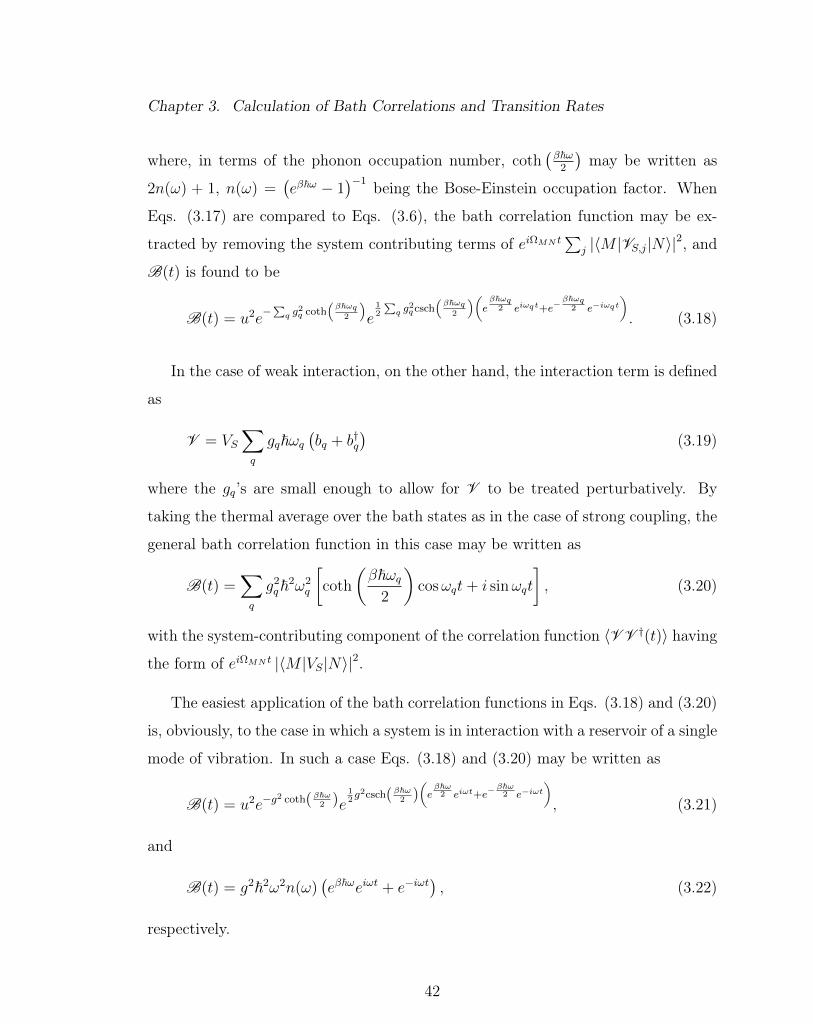
Chapter 3. Calculation of Bath Correlations and Transition Rates
where, in terms of the phonon occupation number, coth(β~ω
2
)may be written as
2n(ω) + 1, n(ω) =(eβ~ω − 1
)−1 being the Bose-Einstein occupation factor. When
Eqs. (3.17) are compared to Eqs. (3.6), the bath correlation function may be ex-
tracted by removing the system contributing terms of eiΩMN t∑
j |〈M |VS,j|N〉|2, and
B(t) is found to be
B(t) = u2e−∑q g
2q coth
(β~ωq
2
)e
12
∑q g
2qcsch
(β~ωq
2
)(eβ~ωq
2 eiωqt+e−β~ωq
2 e−iωqt). (3.18)
In the case of weak interaction, on the other hand, the interaction term is defined
as
V = VS∑q
gq~ωq(bq + b†q
)(3.19)
where the gq’s are small enough to allow for V to be treated perturbatively. By
taking the thermal average over the bath states as in the case of strong coupling, the
general bath correlation function in this case may be written as
B(t) =∑q
g2q~2ω2
q
[coth
(β~ωq
2
)cosωqt+ i sinωqt
], (3.20)
with the system-contributing component of the correlation function 〈V V †(t)〉 having
the form of eiΩMN t |〈M |VS|N〉|2.
The easiest application of the bath correlation functions in Eqs. (3.18) and (3.20)
is, obviously, to the case in which a system is in interaction with a reservoir of a single
mode of vibration. In such a case Eqs. (3.18) and (3.20) may be written as
B(t) = u2e−g2 coth(β~ω2 )e
12g2csch(β~ω2 )
(eβ~ω
2 eiωt+e−β~ω
2 e−iωt), (3.21)
and
B(t) = g2~2ω2n(ω)(eβ~ωeiωt + e−iωt
), (3.22)
respectively.
42

Chapter 3. Calculation of Bath Correlations and Transition Rates
Although the generalized forms of the bath correlation functions in Eqs. (3.18)
and (3.20) in the two respective interaction regimes may be easily applied to in-
teractions with multiple discrete modes, interest also lies in the interaction with a
continuum of modes or phonon bands. In the next Section, an extension of the bath
correlations from a discrete sum to the continuum is made, explicitly.
3.3.1 Phonon Baths
In extending the interaction of a system with a bath of phonons from an inter-
action with discrete modes to an interaction with a continuous band of phonons,
quantitities such as the phonon dispersion relation and the phonon density of states
must be known. In refs. [18, 48, 56], Andersen et. al. studied the interaction of
a 1-dimensional infinite lattice with both acoustic and optical phonon bands for
physically relevant dispersion relations, typical examples of which may be found in
textbooks such as refs. [10] or [57] (see Fig. 3.1). One naturally extends the discrete
sum over the modes to the continuum description, wherein an integration of the
modes over the first Brillouin zone is made,∑q
→ Vν(2π)ν
∫BZ
dq. (3.23)
Here the mode is represented in its wavevector form on the right hand side of Eq.
(3.23) to generalize the transformation corresponding to the dimensionality ν of
the problem, with Vν being the ν-dimensional volume. For simplicity, the coupling
constants gq are taken to be mode-independent in the transformation for the case
of interaction with optical phonons and are taken to be represented by an average
coupling constant g. In general, however, the gq’s are functions of the modes and
associated frequency and are here taken to be represented by an average coupling
constant g multiplied by a frequency dependent function, or, put simply, gq → g(ωq).
In this process all of the ωq’s in the discrete sum are replaced by the corresponding
43

Chapter 3. Calculation of Bath Correlations and Transition Rates
Figure 3.1: Plotted are examples of the one- and two-dimensional dispersion rela-tions commonly found in texts such [10] for optical and acoustic phonons for thefirst Brillouin zone. Seen in the figure are the peak (ω0) and maximum (ωmax,(x,y))frequencies of the optical and acoustic branches, respectively.
dispersion relation ω(q) for the type of phonons considered. General results for the
multi-dimensional memories may be found, for instance, in refs. [18, 48], the results
of which are of particular interest in analyzing charge transport along a specific
principal axis or crystallographic direction of a molecular aggregate.
Further progress is made by the continuum approximation over the modes
∑q
g2q →
∫dω′ g2 (ω′) ρ (ω′) , (3.24)
where ρ (ω′) represents the expression for the frequency density of states involved.
The limits on the integration are placed according to the context of the problem.
With the approximation made in Eq. (3.24), the general bath correlation functions
in Eqs. (3.18) and (3.20) may be written as
B(t) = u2e−∫dω′ g2(ω′)ρ(ω′) coth
(β~ω′
2
)
× e12
∫dω′ g2(ω′)ρ(ω′) csch
(β~ω′
2
)(eβ~ω′
2 eiω′t+e−
β~ω′2 e−iω
′t), (3.25)
44

Chapter 3. Calculation of Bath Correlations and Transition Rates
and
B(t) = ~2
∫dω′ g2 (ω′) ρ (ω′) ω′2
[coth
(β~ω′
2
)cos (ω′t) + i sin (ω′t)
], (3.26)
respectively.
In the next two sections, discussions of the interaction of a system with an optical
and an acoustic phonon band will be made through the use of corresponding density
of states relations, and calculations of the bath correlation functions will be reported
for both interaction strength regimes.
3.3.2 Optical Phonon Band
In the case in which the reservoir is composed of optical phonons, the density of
states may be considered to be that of a Gaussian peaked at a frequency ω0 and
width σ ω0, and the coupling constants gq to be represented by their average, g,
such that
g2(ω)ρ(ω′) =g2
√2π σ
e−(ω′−ω0)2
2σ2 . (3.27)
If σ is small enough with respect to ω0, one may ignore the cutoff of ρ(ω′) and invoke
the approximation that ω′ extends to ±∞. On substituting this density of states
into the expressions for the bath correlation functions in Eqs. (3.18) and (3.20), we
get
B(t) = u2e−g2 coth(β~ω0
2 )(
1−e−σ2t2
2 cosω0t
)eig
2e−σ2t2
2 sinω0t, (3.28)
in the strong-coupling case [58] and
B(t) = g2~2ω20e−σ
2t2
2
×
coth
(β~ω0
2
)[(1 +
σ2
ω20
− σ4t2
ω20
)cos (ω0t)− 2
σ2
ω0
t sin (ω0t)
]
+ i
[(1 +
σ2
ω20
− σ4t2
ω20
)sin (ω0t) + 2
σ2
ω0
t cos (ω0t)
], (3.29)
45
Chapter 3. Calculation of Bath Correlations and Transition Rates
in the weak-coupling case, respectively. The forms of the functions in Eq. (3.28) and
(3.29) are obtained after the integration limits are appropriately taken to be infinite
through the narrow band assumption placed on the Gaussian form of the phonon
density of states, σ ω0 [58]. If the Gaussian width σ is taken to be infinitesimally
small such that the Gaussian density of states may be faithfully represented by a
delta function and all dependence on the width σ disappears, the forms of the bath
correlation functions describing the interaction with a single mode of vibration in Eqs.
(3.21) and (3.22) are faithfully reproduced from Eqs. (3.28) and (3.57), respectively.
Another form which may be considered for the frequency density of states to
represent a band of optical phonons peaked at a frequency ω0 is that of a Lorentzian
with narrow width α ω0:
ρ(ω′) =1
π
α
α2 + (ω′ − ω0)2 . (3.30)
This particular density of states yields similar expressions for the bath correlation
functions to those in Eqs. (3.28) and (3.29) of
B(t) = u2e−g2 coth(β~ω0
2 )(1−e−αt cosω0t)eig2e−αt sinω0t, (3.31)
in the strong-coupling case [58] and
B(t) = g2~2ω20
(1− i α
ω0
)2
e−αt[coth
(β~ω0
2
)cos (ω0t) + i sin (ω0t)
], (3.32)
in the weak-coupling case, respectively. Under the right circumstances, the interac-
tion with a band of optical phonons may be appropriately described and represented
by the interaction with a single mode of vibration [18] as will be seen later on in this
study.
3.3.3 Acoustic Phonon Band
While the focus in this thesis is mainly on the interaction of a nondegenerate system
with optical phonons, interesting results are obtained when a bath consisting of
46

Chapter 3. Calculation of Bath Correlations and Transition Rates
acoustic phonons is considered. In the case of an interaction with an acoustic phonon
band, the product of the coupling constant with the phonon density of states may
be taken, in combination with the deformation potential approximation [56], to be
that depicted by the Debye model
g2(ω)ρ(ω′) =g2
ωmax
(ω′
ωmax
)dΘ (ωmax − ω′) (3.33)
where ωmax is the maximum cutoff frequency determined by the characteristics of
the bath and ν = d + 1 determines the dimensionality of the problem (e.g., if the
problem is 1-dimensional, d = 0 and ν = 1), consistent with the Debye formulation.
Substitution of Eq. (3.33) into the bath correlation functions of Eqs. (3.20) and
(3.18) yields
B(t) = u2e−g2
ν e−2g2 Γ(ν)
(β~ωmax)ν
[ζ(ν)−
∑ν−1n=0
(β~ωmax)n
n!Liν−n(e−β~ωmax)
]
× eg2 Γ(ν)
(β~ωmax)ν (ζ(ν,−i tβ~)+ζ(ν,1+i tβ~))
× e−g2Γ(ν)
∑ν−1n=0
(β~ωmax)n−νn!
eiωmaxtΦ(e−β~ωmax ,ν−n,−i tβ~)
× e−g2Γ(ν)
∑ν−1n=0
(β~ωmax)n−νn!
e−β~ωmaxe−iωmaxtΦ(e−β~ωmax ,ν−n,1+i tβ~), (3.34)
in the case of a strong coupling between the system and phonons and
B(t) =g2~2ω2
max
(β~ωmax)ν+2 Γ (ν + 2)
×
ζ
(ν + 2,−i t
β~
)+ ζ
(ν + 2, 1 + i
t
β~
)
−ν+1∑n=0
(β~ωmax)n
n!
[e−iωmaxte−β~ωmaxΦ
(e−β~ωmax , ν − n+ 2, 1 + i
t
β~
)
+ eiωmaxtΦ
(e−β~ωmax , ν − n+ 2,−i t
β~
)], (3.35)
in the case of weak coupling. In both cases Γ(ν) is the gamma function, γ (n, x) is the
lower incomplete gamma function, ζ(ν) =∑∞
k=1 k−ν is the Riemann zeta function,
ζ(ν, x) =∑∞
k=0 (k + x)−ν is the Hurwitz zeta function, Lis(x) =∑∞
k=1 xk k−ν is the
47

Chapter 3. Calculation of Bath Correlations and Transition Rates
Figure 3.2: The real (solid) and imaginary (dashed) components of the Lerch tran-scendent (top left), Hurwitz zeta (bottom left), polylogarithm (top right), and lowerincomplete gamma (bottom right) functions are plotted for three dimensions, ν = 1,2, and 3. The two components of the Lerch transcendent for a fixed finite temperaturedecay with time for all three dimensions. The Hurwitz zeta function, correspondingto the Lerch transendent with the first argument being unity, has similar behaviorfor the two higher dimensions, but for 1 dimension, the imaginary component has anonzero asymptotic value. The real and imaginary components of the lower incom-plete gamma function are seen to oscillate, increasing in amplitude, with time, whilethe polylogarithm function increases from zero at zero temperature to an associatedasymptotic value for each dimension with zero imaginary component.
polylogarithm function, and Φ(x, ν, a) =∑∞
k=0 xk (k + a)−ν is the Lerch transcen-
dent. It is worthy to note here that while the Riemann zeta function evaluated at
ν = 1 diverges, its Cauchy principal value determined by
limε→0
ζ (1 + ε) + ζ (1− ε)2
(3.36)
is a finite value given by the Euler–Mascheroni constant γ = 0.5772... [59].
The Lerch transcendent as a function is the generalization of both the Hurwitz
zeta and polylogarithm functions. For the particular case under study here the first
term in the Lerch transcendent varies only between 0 and 1, eliminating certain
48
Chapter 3. Calculation of Bath Correlations and Transition Rates
behaviors and allowing for more straightforward analysis. In this case the general
form of the first term in the Lerch transcendent is e−β~ωmax . If the first term is 1
corresponding to the case of high temperature, the behavior is governed by that of
the Hurwitz zeta function. If, on the other hand, the first argument approaches 0
corresponding to low temperature, the Lerch transcendent approaches a−ν and the
time-dependence of the bath correlation functions in this case would be defined by
the behavior of their temperature independent components, i.e.,
B(t) = u2e−g2
[1ν−Γ(ν)eiωmaxt
∑ν−1n=0
(−iωmaxt)n−ν
n!
], (3.37)
in the case of strong coupling and
B(t) = g2~2ω2maxΓ (ν + 2) eiωmaxt
ν+1∑n=0
(−i)n−ν (ωmaxt)n−ν−2
n!, (3.38)
in the case of weak coupling, respectively.
If the temperature dependence of the last term in the Lerch transcendent and
Hurwitz zeta functions in Eqs. (3.34) and (3.35) is also considered, it is made clear
that the limiting forms of the Lerch transcendent for this particular applied case
are 1 for the case of zero temperature and the corresponding value of the Hurwitz
zeta function in the case of high temperature, which is either zero or a finite value
depending on the dimensionality of the problem considered. For finite temperatures,
the real part of the Lerch transcendent has the specific property that it decreases
from a finite, nonzero value and eventually decays to zero with time. The imaginary
part, on the other hand, starts at a zero value, becomes either positive or negative
depending on the sign in front of t in the third argument of the Lerch transcendent,
and returns to zero with time. Combining the behavior of the four special functions
considered in the definition of the associated bath correlation functions along with
their products with time- and temperature-dependent algebraic functions reveals
intriguing properties in the behavior of the memories and transition rates for the
case of the interaction with acoustic phonons as will be seen in later Sections.
49

Chapter 3. Calculation of Bath Correlations and Transition Rates
3.4 Effects of Strong Coupling - Dressed Bath Cor-
relation Functions
In much of the previous literature [48, 58, 60–62] used as guidance in present calcu-
lations, the strong interaction of a system with a single mode of vibration has been
analyzed with some extensions made later to approximate and exact forms of the
interactions with optical phonon bands. The system particular to all of the calcula-
tions present in the literature is that of the spin-boson [61] or nondegenerate dimer
[62]. For such systems (as will be seen in Chapter 4), the system matrix elements,
|〈M |VS|N〉|2 in the weak-coupling case and∑
j |〈M |VS,j|N〉|2 in the strong-coupling
case, when summed over all states N 6= M in the GME (Eq. (2.9)) reduce to either
unity or state dependent terms which do not contribute to the post-summation re-
sulting memories which describe the energetically upward and downward transitions.
In the case in which only nearest-neighbor transitions are considered, a perturba-
tive treatment involving powers of the interaction results in vanishing memories if
M − N 6= ±1. In such a prescribed situation, the frequency ΩMN defined by the
energy difference between the system energy levels M and N is taken as ±Ω if M
and N are neighboring energy states and is taken to be the same throughout. The
memories describing the energetically upward and downward transitions of a system
coupled to a single mode of vibration may then be written as [58]
W±(t) = 2u2
~2e−g
2 coth(β~ω2 )(1−cosωt) cos(g2 sinωt± Ωt
), (3.39)
in the strong-coupling regime and
W±(t) = 2g2ω2
[coth
(β~ω
2
)cos (ωt) cos (Ωt)∓ sin (ωt) sin (Ωt)
], (3.40)
in the weak-coupling regime, where the + and − signs indicate energetically upward
and downward transitions, respectively.
It is expected that the memory functions resulting from the use of Eqs. (3.39)
50

Chapter 3. Calculation of Bath Correlations and Transition Rates
Figure 3.3: The memories corresponding to the energetically upward and downwardtransitions of a system of characteristic frequency Ω in strong interaction (g = 2)with a single mode of vibration of frequency ω = Ω, non-decaying (left) and thoseincorporating disorder α = 0.01ω (right), are plotted with respect to time withT = ~ω/kB. The plots for the degenerate case are given in ref. [58].
and (3.40) would decay to zero at long times due to the interaction of the system
with the thermal reservoir, however, the linear interactions considered in this study
cannot broaden the zero-phonon lines present in optical spectra [17, 55], and the
memories produced never quite decay to zero, producing infinite rates. The solution
to this problem, discussed in the literature earlier [18,55], lies in the unavoidable in-
troduction of sources of disorder not taken explicitly into account in the microscopic
description of the Hamiltonian [44, 45, 50–55]. This is done through the incorpora-
tion of an extra time-dependent decay factor f(t) introduced into the memories [18]
which takes into account both the phonon spectral line shape and sources of disor-
der mentioned above. The most convenient representation of f(t) is the exponential
e−αt which is compatible with the derivation of the GME in the presence of disorder
[63, 64] and corresponds to an ideal spectral line shape of a Lorentzian in the fre-
quency domain [17]. This form of f(t) allows for the memories in Eqs. (3.39) and
51

Chapter 3. Calculation of Bath Correlations and Transition Rates
Figure 3.4: The memories corresponding to the energetically upward and downwardtransitions of a system of characteristic frequency Ω in weak interaction (g = 0.02)with a single mode of vibration of frequency ω = Ω, non-decaying (left) and thoseincorporating disorder α = 0.01ω (right), are plotted with respect to time withT = ~ω/kB.
(3.40) to be better represented by the forms
W±(t) = 2u2
~2e−g
2 coth(β~ω2 )(1−cosωt) cos(g2 sinωt± Ωt
)e−αt, (3.41)
in the strong-coupling regime and
W±(t) = 2g2ω2
[coth
(β~ω
2
)cos (ωt) cos (Ωt)∓ sin (ωt) sin (Ωt)
]e−αt, (3.42)
in the weak-coupling regime, respectively.
While the unavoidable introduction of the damping factor e−αt in Eqs. (3.39)
and (3.40) is essential to avoid infinities, which corresponds to the nonzero steady-
state value of the memories in the time-domain [17, 55], the use of a single α for
all transitions introduces its own inaccuracy. In particular, when the respective
energetically upward (+) and downward (−) transition rates Γ± are calculated, it is
evident that strict detailed balance fails for certain temperature intervals. As will be
discussed in Chapter 5, the remedy lies in coarsening the description in ω-space and
52
Chapter 3. Calculation of Bath Correlations and Transition Rates
considering the Lorentzians present in the transition rates as rectangular functions of
narrow width α centered about each corresponding frequency $ along the spectrum,
i.e.,
1
π
α
α2 +$2≈ 1
αrect
($α
)=
1
α
[Θ($ +
α
2
)−Θ
($ − α
2
)]. (3.43)
The transition rates Γ±, found by taking the Fourier transform of the specified mem-
ories in Eqs. (3.41) and (3.42), as
Γ± =2
π
u2
~2e−g
2 coth(β~ω02 )
∞∑`=−∞
I`[2g2n (ω0)
] ∞∑k=0
g2k
k!
α
α2 + [(k + `)ω0 ± Ω]2(3.44)
in the multiphonon (strong-coupling) interaction case, and
Γ± =2
πg2ω2
0
[n (ω0) + 1]
α
α2 + (ω0 ± Ω)2 + n (ω0)α
α2 + (ω0 ∓ Ω)2
(3.45)
in the single-phonon (weak-coupling) interaction case, respectively, may be written
in terms of rectangular functions as
Γ± = 2u2
~2αe−g
2 coth(β~ω02 )
∞∑`=−∞
I`[2g2n (ω0)
] ∞∑k=0
g2k
k!rect
((k + `)ω0 ± Ω
α
)(3.46)
in the multiphonon (strong-coupling) interaction case, and
Γ± = 2g2ω20
α
[n (ω0) + 1] rect
(ω0 ± Ω
α
)+ n (ω0) rect
(ω0 ∓ Ω
α
)(3.47)
in the single-phonon (weak-coupling) case, respectively.
With the forms of the rates in Eqs. (3.46) and (3.47) detailed balance between
the energetically upward and downward transition rates is restored (see discussion
in Chapter 5) as the narrow peaks (or table tops) and sharp drop off of the rectangu-
lar functions to zero ensure that detailed balance is maintained along the frequency
spectrum for all T . Both representations of the transition rates in each of the two
interaction regimes exhibit the same behavior in terms of their temperature depen-
dence (see Fig. 3.5). In the case of weak interaction with the bath (single-phonon
53

Chapter 3. Calculation of Bath Correlations and Transition Rates
Figure 3.5: The transitions rates Γ are plotted with respect to temperature T in unitsof ~Ω/kB for a system of characteristic frequency Ω in strong (g = 2, left panel) andweak (g = 0.02, right panel) interaction with a single mode of vibration of frequencyω = Ω with the incorporation of disorder α = 0.01ω. A monotonic increase of therate with increasing T is observed for the weak-coupling (single-phonon) interactioncase, while the behavior of the rate in the strong-coupling (multiphonon) case exhibitsdistinctive nonmonotonic behavior with increasing T , making the T interval overwhich the rate is observed of particular importance.
interaction), the rates exhibit an Arrhenius behavior with temperature wherein the
rate is activated and increases with increasing temperature. In the case of a strong-
coupling (multiphonon) interaction the Arrhenius behavior is also present but then a
nonmonotonic behavior of the rate is observed, the increasing and decreasing behav-
ior of the transition rates for both representative versions (Eqs. (3.44) and (3.46))
being determined by the temperature interval over which the rates are observed.
3.4.1 Optical Phonon Band
In the case in which there is a strong interaction between a system of characteristic
frequency Ω and an optical band of phonons described by a Gaussian density of
54

Chapter 3. Calculation of Bath Correlations and Transition Rates
states, the bath correlation function in Eq. (3.28) is substituted into Eqs. (3.4)
to find expressions for the memories describing energetically upward and downward
transitions, the memories having the forms
W±(t) = 2u2
~2e−g2 coth(β~ω0
2 )(
1−e−σ2t2
2 cosω0t
)cos(g2e−
σ2t2
2 sinω0t± Ωt). (3.48)
Here, it is easy to show that as σ tends to 0 the expressions for the memories for the
case of strong interaction with a single mode of vibration may be reproduced (see
Eq. (3.39)). Unlike in the case of strong interaction with a single mode of vibration,
wherein the memories obtained in Eqs. (3.39) and (3.40) never decay, it appears
that the “natural” decay introduced through the dispersion evident in the shape of
the phonon spectral line allows for a more physical result to be obtained without the
need for the insertion of a superficial decay parameter such as that of the disorder
introduced in Eqs. (3.41) and (3.42) [18].
The memories in Eqs. (3.48) exhibit an overall decay of their peak amplitudes
(see Fig. 3.6), as the decay is governed by a Gaussian-like envelope function of the
form,
Wenvelope(t) 2u2
~2e−g
2 coth(β~ω02 )σ2t2 . (3.49)
This type of decay limits the fluctuations between transitions to a time scale that
is temperature-dependent and of the form τγ =[g2 coth
(β~ω0
2
)σ2]−1/2
. Inside the
decay envelope, muted and revived oscillations are apparent, each corresponding to
a specific time scale, the period of the rapid oscillations being characterized by the
argument inside of the downstairs cosine of the memories in Eq. (3.48) [58,61].
It is important to note here that, although it seems that the memories decay
to zero at long times (see Fig. 3.6), the memories produced via the direct Fourier
transform of the phonon density of states never quite dissipate to zero (see lower
left inset of Fig. 3.6). This type of non-decaying behavior corresponds to a closed
system which inhibits the full dissipation of the system’s energy to the surroundings.
55
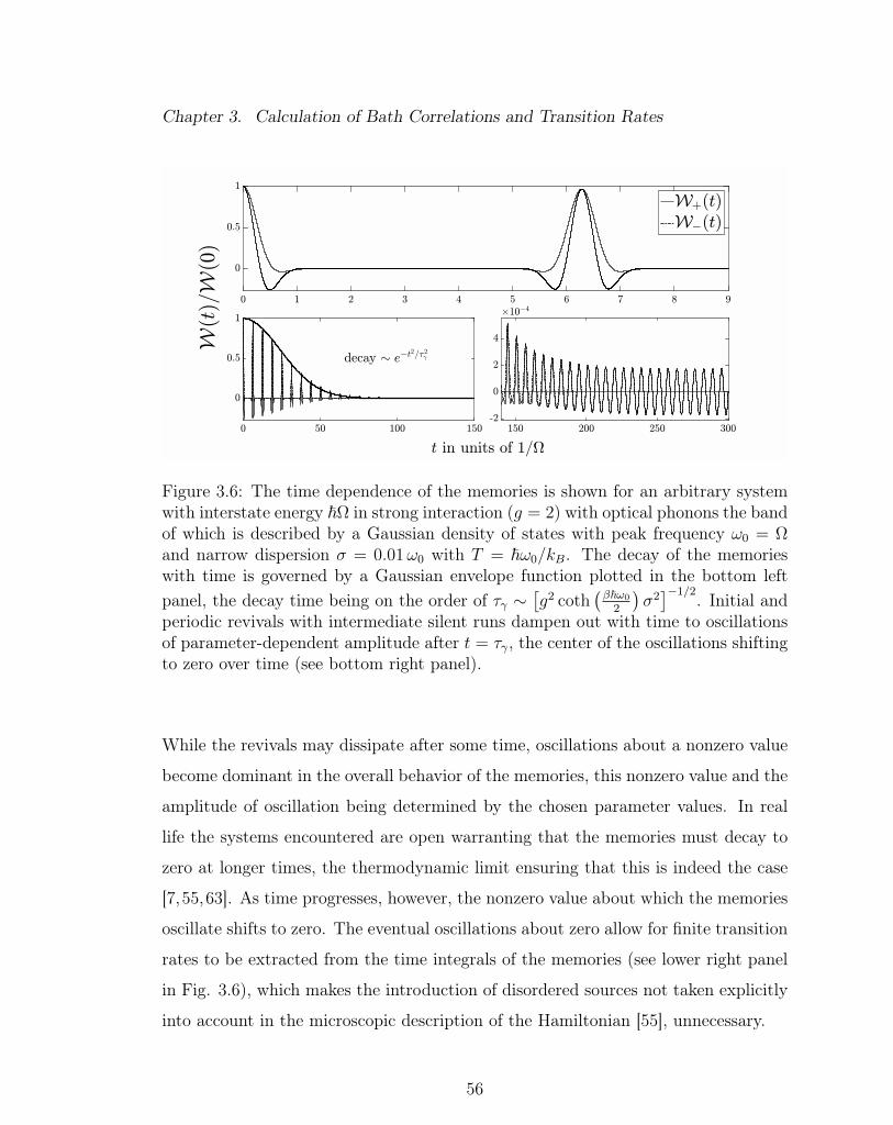
Chapter 3. Calculation of Bath Correlations and Transition Rates
Figure 3.6: The time dependence of the memories is shown for an arbitrary systemwith interstate energy ~Ω in strong interaction (g = 2) with optical phonons the bandof which is described by a Gaussian density of states with peak frequency ω0 = Ωand narrow dispersion σ = 0.01ω0 with T = ~ω0/kB. The decay of the memorieswith time is governed by a Gaussian envelope function plotted in the bottom leftpanel, the decay time being on the order of τγ ∼
[g2 coth
(β~ω0
2
)σ2]−1/2
. Initial andperiodic revivals with intermediate silent runs dampen out with time to oscillationsof parameter-dependent amplitude after t = τγ, the center of the oscillations shiftingto zero over time (see bottom right panel).
While the revivals may dissipate after some time, oscillations about a nonzero value
become dominant in the overall behavior of the memories, this nonzero value and the
amplitude of oscillation being determined by the chosen parameter values. In real
life the systems encountered are open warranting that the memories must decay to
zero at longer times, the thermodynamic limit ensuring that this is indeed the case
[7,55,63]. As time progresses, however, the nonzero value about which the memories
oscillate shifts to zero. The eventual oscillations about zero allow for finite transition
rates to be extracted from the time integrals of the memories (see lower right panel
in Fig. 3.6), which makes the introduction of disordered sources not taken explicitly
into account in the microscopic description of the Hamiltonian [55], unnecessary.
56
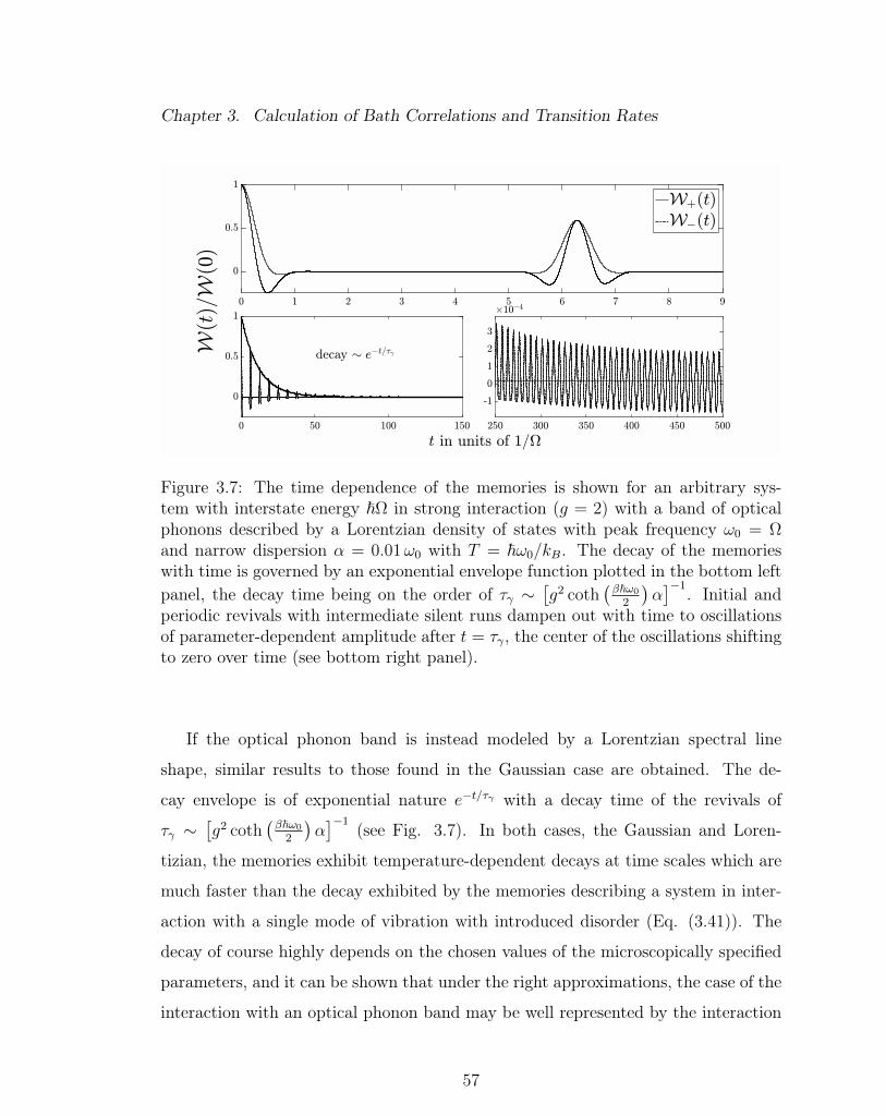
Chapter 3. Calculation of Bath Correlations and Transition Rates
Figure 3.7: The time dependence of the memories is shown for an arbitrary sys-tem with interstate energy ~Ω in strong interaction (g = 2) with a band of opticalphonons described by a Lorentzian density of states with peak frequency ω0 = Ωand narrow dispersion α = 0.01ω0 with T = ~ω0/kB. The decay of the memorieswith time is governed by an exponential envelope function plotted in the bottom leftpanel, the decay time being on the order of τγ ∼
[g2 coth
(β~ω0
2
)α]−1
. Initial andperiodic revivals with intermediate silent runs dampen out with time to oscillationsof parameter-dependent amplitude after t = τγ, the center of the oscillations shiftingto zero over time (see bottom right panel).
If the optical phonon band is instead modeled by a Lorentzian spectral line
shape, similar results to those found in the Gaussian case are obtained. The de-
cay envelope is of exponential nature e−t/τγ with a decay time of the revivals of
τγ ∼[g2 coth
(β~ω0
2
)α]−1
(see Fig. 3.7). In both cases, the Gaussian and Loren-
tizian, the memories exhibit temperature-dependent decays at time scales which are
much faster than the decay exhibited by the memories describing a system in inter-
action with a single mode of vibration with introduced disorder (Eq. (3.41)). The
decay of course highly depends on the chosen values of the microscopically specified
parameters, and it can be shown that under the right approximations, the case of the
interaction with an optical phonon band may be well represented by the interaction
57

Chapter 3. Calculation of Bath Correlations and Transition Rates
Figure 3.8: Plots of the spectral function (left panel) and energetically upward (Γ+)and downward (Γ−) transition rates (right panels) are presented for the case of asystem of characteristic frequency Ω in strong interaction (g = 2) with a bath ofoptical phonons with average frequency ω0 = Ω and narrow dispersion σ = 0.01ω0
for T = ~ω0/kB. The spectral function and rates are plotted with respect to thefrequency z in units of ω0, and temperature T in units of T0, respectively, whereT0 = ~ω0/kB is the vibrational temperature. Multiple peaks are visible in Y(z), eachpeak with a corresponding center, width, and magnitude. The upward and downwardtransition rates are shown to satisfy detailed balance for all T . A nonmonotonicbehavior with T is evident in the rates, showing the importance of the chosen Tinterval over which the rates are observed.
with a single mode of vibration with the interaction of disorder to the model [18].
Transition Rates
The bath spectral function corresponding to the bath correlation function of Eq.
(3.28) describing a system in strong interaction with a bath of optical phonons of
peak frequency ω0 and narrow dispersion σ, with a continuous and infinite band of
frequencies, has the general form of
58

Chapter 3. Calculation of Bath Correlations and Transition Rates
Y(z) = 2u2
~2
e−g2 coth(β~ω0
2 )√
2π
×∞∑
`=−∞
∞∑m=0
[g2
2csch
(β~ω0
2
)]2m+|`|
m!Γ (m+ |`|+ 1)
e`β~ω0
2 e− [z−(Ω+`ω0)]2
2(2m+|`|)σ2√2m+ |`|σ
. (3.50)
The shape of the spectral function is governed by multiple Gaussian peaks (see Fig.
3.8), which are equidistant from each other in the frequency domain by one unit of ω0
and describe transitions between quantized vibrational states. Each peak corresponds
to a particular vibrational transition within the phonon bath and the associated
peak magnitude, which is related to the transition probability of the occurrence of
the corresponding transition, reveals information about the occupation population of
the levels involved in the transition. The center of each peak nω0 = ∆ε is the central
frequency corresponding to the associated vibrational transtion involved and the
natural linewidth of each peak determines the lifetime of the associated vibrational
state which is on the order of ∼[2√
2 ln 2σ]−1
. The narrow linewidths presented in
Fig. 3.8 correspond to long lifetimes which is in agreement with the experimental
observations of long-lived spontaneous vibrational states [1].
The associated rates describing the rate of the energetically upward or downward
transitions for a given system of equally spaced energy levels have the forms
Γ± =√
2πu2
~2e−g
2 coth(β~ω02 )
×∞∑
`=−∞
∞∑m=0
[12g2csch
(β~ω0
2
)]2m+|`|e±`
β~ω02 e
− (Ω+`ω0)2
2(2m+|`|)σ2
m!Γ (m+ |`|+ 1)√
(2m+ |`|)σ. (3.51)
The right two panels of Fig. 3.8 show the temperature dependence of the rates
described in the expressions of Eqs. (3.51). The nonmonotonic temperature depen-
dence of the rates is reminiscent of that observed for the case of a strong interaction
with a single mode of vibration with the inclusion of disordered sources. Here, how-
ever, the nonmonotonicity is further exaggerated as the rates change and shift more
abruptly with varying temperature further emphasizing how the relaxation behavior
59

Chapter 3. Calculation of Bath Correlations and Transition Rates
of a system may be affected by the strength of the interaction with and the details
of the microscopically specified reservoir. The bottom right panel of Fig. 3.8 verifies
that strict detailed balance is conserved for all temperatures as guaranteed by the
shape of the properties of the Gaussian peaks in Y(z), a feature which is not present
in Lorentzian functions.
If, instead, use is made of the bath correlation function in Eq. (3.31), wherein
the spectral line shape of the optical phonons is described by a Lorentzian, the bath
spectral function is found to have the form
Y(z) =2
π
u2
~2e−g
2 coth(β~ω02 )
×∞∑
`=−∞
∞∑m=0
[g2
2csch
(β~ω0
2
)]2m+|`|
m!Γ (m+ |`|+ 1)
(2m+ |`|)α e`β~ω0
2
(2m+ |`|)2 α2 + [z − (Ω + `ω0)]2.
(3.52)
The shape of the spectral function in this case is governed by multiple Lorentzian
peaks in the frequency domain as seen in the left panel of Fig. 3.9, each with a center
at a corresponding value of z = nω0 and a width determined by a respective value
which determines the lifetime of the associated transition. In this model, the lifetime
is on the order of (2α)−1. The rates associated with the energetically upward or
downward transitions for a given system of equally spaced energy levels in this case
have the forms
Γ± = 2u2
~2e−g
2 coth(β~ω02 )
×∞∑
`=−∞
∞∑m=0
[12g2csch
(β~ω0
2
)]2m+|`|
m!Γ (m+ |`|+ 1)
(2m+ |`|)α e±`β~ω0
2
(2m+ |`|)2 α2 + (Ω + `ω0)2 . (3.53)
The right two panels of Fig. 3.9 show the temperature dependence of the rates
described in the expressions of Eqs. (3.51). As in the case of a strong interaction
with a single mode with the inclusion of disordered sources and the case in which
the optical phonons are represented by a Gaussian spectral line shape, the rates are
60
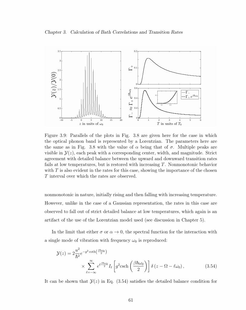
Chapter 3. Calculation of Bath Correlations and Transition Rates
Figure 3.9: Parallels of the plots in Fig. 3.8 are given here for the case in whichthe optical phonon band is represented by a Lorentzian. The parameters here arethe same as in Fig. 3.8 with the value of α being that of σ. Multiple peaks arevisible in Y(z), each peak with a corresponding center, width, and magnitude. Strictagreement with detailed balance between the upward and downward transition ratesfails at low temperatures, but is restored with increasing T . Nonmonotonic behaviorwith T is also evident in the rates for this case, showing the importance of the chosenT interval over which the rates are observed.
nonmonotonic in nature, initially rising and then falling with increasing temperature.
However, unlike in the case of a Gaussian representation, the rates in this case are
observed to fall out of strict detailed balance at low temperatures, which again is an
artifact of the use of the Lorentzian model used (see discussion in Chapter 5).
In the limit that either σ or α→ 0, the spectral function for the interaction with
a single mode of vibration with frequency ω0 is reproduced:
Y(z) = 2u2
~2e−g
2 coth(β~ω02 )
×∞∑
`=−∞
e`β~ω0
2 I`
[g2csch
(β~ω0
2
)]δ (z − Ω− `ω0) , (3.54)
It can be shown that Y(z) in Eq. (3.54) satisfies the detailed balance condition for
61
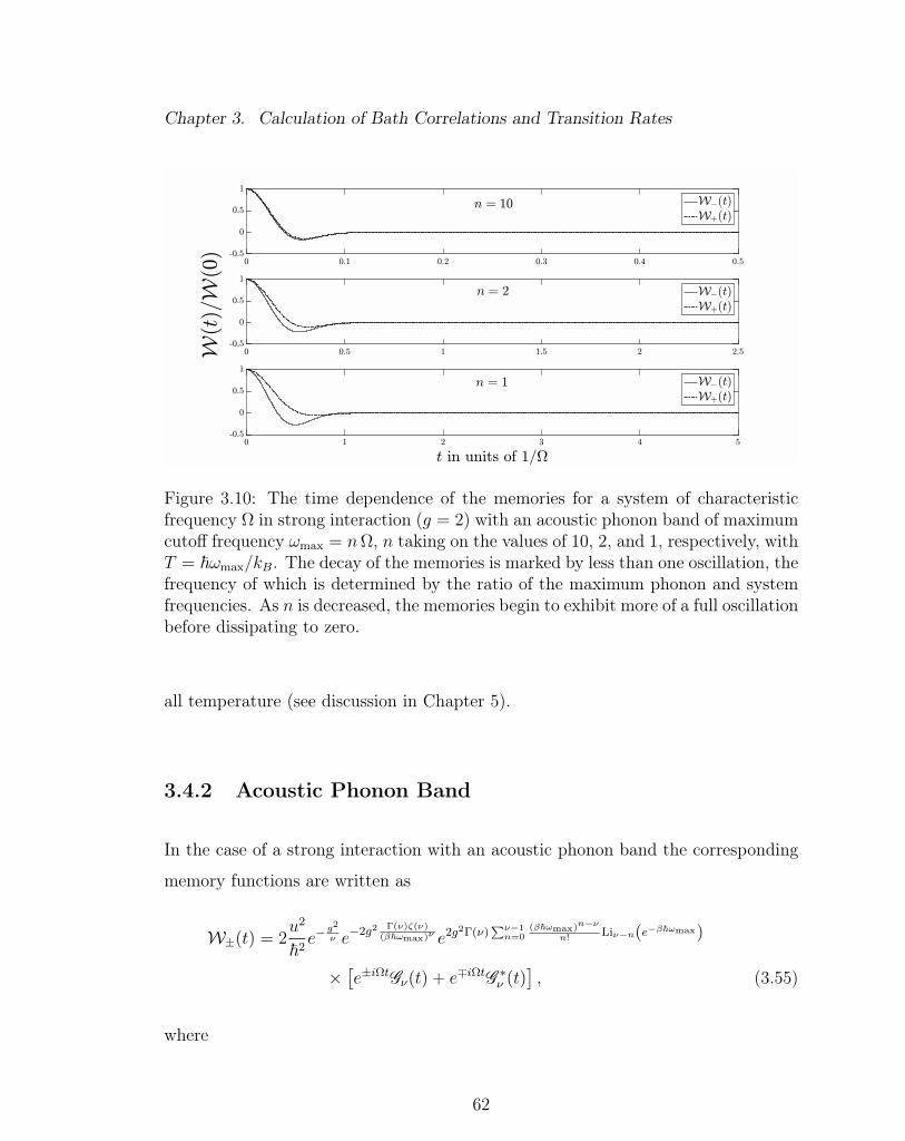
Chapter 3. Calculation of Bath Correlations and Transition Rates
Figure 3.10: The time dependence of the memories for a system of characteristicfrequency Ω in strong interaction (g = 2) with an acoustic phonon band of maximumcutoff frequency ωmax = nΩ, n taking on the values of 10, 2, and 1, respectively, withT = ~ωmax/kB. The decay of the memories is marked by less than one oscillation, thefrequency of which is determined by the ratio of the maximum phonon and systemfrequencies. As n is decreased, the memories begin to exhibit more of a full oscillationbefore dissipating to zero.
all temperature (see discussion in Chapter 5).
3.4.2 Acoustic Phonon Band
In the case of a strong interaction with an acoustic phonon band the corresponding
memory functions are written as
W±(t) = 2u2
~2e−
g2
ν e−2g2 Γ(ν)ζ(ν)(β~ωmax)ν e2g2Γ(ν)
∑ν−1n=0
(β~ωmax)n−νn!
Liν−n(e−β~ωmax)
×[e±iΩtGν(t) + e∓iΩtG ∗ν (t)
], (3.55)
where
62

Chapter 3. Calculation of Bath Correlations and Transition Rates
Gν(t) = eg2 Γ(ν)
(β~ωmax)ν (ζ(ν,−i tβ~)+ζ(ν,1+i tβ~))
× e−g2Γ(ν)
∑ν−1n=0
(β~ωmax)n−νn!
eiωmaxtΦ(e−β~ωmax ,ν−n,−i tβ~)
× e−g2Γ(ν)
∑ν−1n=0
(β~ωmax)n−νn!
e−β~ωmaxe−iωmaxtΦ(e−β~ωmax ,ν−n,1+i tβ~). (3.56)
The 1-dimensional case of Eq. (3.55) is shown in Fig. 3.10 for three respective values
of n = ωmax/Ω. In each case, the memories dissipate to zero in about one oscillation
with a period of oscillation determined by the ratio of the maximum phonon fre-
quency to the system frequency. In all three cases the memory corresponding to the
energetically upward transition decays faster to zero than its energetically upward
counterpart. The decay cutoff apparent in all cases is a consequence of the proper-
ties of the bath considered, reinforcing the idea that the characteristics of the bath
determine the behavior of the relaxation of the system.
Transition Rates
The intricate nature of the analytic form of the bath correlation function in Eq.
(3.34) associated with this type of interaction prevents the derivation of an analytic
form for the spectral function, however, the Fourier transform of Eq. (3.34) may
be numerically performed to obtain results for the associated spectral function and
transition rates. Fig. 3.11 shows the numerically obtained spectral function and
transition rates plotted for an arbitrary system exhibiting nearest neighbor transi-
tions.
The form of the spectral function exhibits a single peak that is Gaussian in
nature, having a finite width and a peak value centered at a respective maximum
frequency determined by the value of the parameters. An interesting feature arises
in the behavior of the rates which exhibit an expected Arrhenius-like behavior with
temperature, differing from the nonmonotonic temperature dependence evident in
the case of strong interaction with optical phonons. This is a direct consequence of
63

Chapter 3. Calculation of Bath Correlations and Transition Rates
Figure 3.11: The spectral function (left) and the transition rates (right) for a sys-tem with characteristic frequency Ω in strong interaction (g = 2) with an acousticphonon band of maximum cutoff frequency ωmax = Ω are plotted with respect tothe frequency z in units of ωmax with T = ~ωmax/kB and temperature T in unitsof T0 = ~ωmax/kB, respectively, for ν = 1. The spectral function is marked by asingle peak of finite width which behaves much like a Gaussian, corresponding toa short-lived vibrational state. The rates are shown to exhibit an Arrhenius-likedependence on the temperature and follow, to some extent, detailed balance for agiven T interval.
the form of the density of states considered, which in the 1-dimensional case yields
a constant value along the frequency domain for all frequencies, sampling over the
range between 0 and ωmax. While in most cases it is expected that there will be a
Boltzmann factor resulting from the n(ω) terms determining the behavior of the rates
with temperature, the Debye model chosen to describe the acoustic phonons offers,
much like in the standard statistical mechanics problem of the Debye specific heat but
inverted, a power law in the temperature dependence in addition to the corresponding
Boltzmann factors. This results in the Arrhenius-like nature of the rates observed,
as they increase with increasing temperature. The temperature dependence of the
rates in this case illustrates that the relaxation behavior is not only dependent on
64

Chapter 3. Calculation of Bath Correlations and Transition Rates
the strength of the interaction, but also on the properties of the bath with which the
system is in contact.
3.5 Effects of Weak Coupling - Bare Bath Correla-
tion Functions
For illustration, the simpler and well-understood case in which a system is in weak
interaction with a thermal reservoir will be considered in this Section. In this type
of interaction the rates are generally found to have an Arrhenius temperature de-
pendence through direct dependence on the Bose occupation factors involved in the
prescription, and in turn a direct dependence on the temperature is observed at
higher T . The baths considered will be those mentioned so far in this Chapter which
consist of either optical or acoustic phonons and the resulting memories, bath spec-
tral functions, and rates will be briefly introduced and discussed. As before, the
general system considered is nondegenerate and exhibits only nearest-neighbor tran-
sitions, the energy difference between subsequent states being of equal magnitude
such that the system is characterized by a frequency Ω. Unlike the case of a system
interacting with phonons of a single mode wherein the introduction of disorder was
deemed essential in the analysis, the memories formulated in this Section have the
property of decaying naturally over time due to the nature of the bath introduced in
each case making the introduction of disorder unnecessary.
3.5.1 Optical Phonon Band
In the case of a weak interaction with an optical phonon band, the corresponding
memory functions associated with the description of the phonon density of states by
65

Chapter 3. Calculation of Bath Correlations and Transition Rates
a Gaussian are written as
W±(t) = 2g2ω20n (ω0) e−
σ2t2
2
×
(1 +
σ2
ω20
− σ4t2
ω20
)[eβ~ω0 cos (ω0t± Ωt) + cos (ω0t∓ Ωt)
]− 2
σ2
ω0
t[eβ~ω0 sin (ω0t± Ωt) + sin (ω0t∓ Ωt)
]. (3.57)
In the case in which the band of optical phonons is described by a Lorentzian, on
the other hand, the memories take the form
W±(t) = 2g2ω20n (ω0) e−αt
×
(1− α2
ω20
)[eβ~ω0 cos (ω0t± Ωt) + cos (ω0t∓ Ωt)
]− 2
α
ω0
[eβ~ω0 sin (ω0t± Ωt) + sin (ω0t∓ Ωt)
]. (3.58)
In both cases ω0 is the peak or average frequency of the phonons and the dispersion
is represented by the narrow width which is σ in the Gaussian case and α in the
Lorentzian case. If α or σ is taken to be infinitesimally small, the resulting forms
of the expressions for the memories in both cases would yield the behavior for the
interaction with a single mode of vibration with no disorder.
In Fig. 3.12 the memories in Eqs. (3.57) and (3.58) are plotted showing an
overall decay of the maximum amplitude, the decay of the memories being governed
by either a Gaussian or exponential envelope function of the form
Wenvelope(t) 2g2ω20 coth
(β~ω0
2
)f(t),
where f(t) = e−σ2t2
2 or e−αt depending on the phonon density of states considered in
representing the bath. An interesting feature arises in the form of the memories in
both representations, that feature being the disparity in the amplitude of oscillation
between the memories describing the energetically upward and downward transitions.
66

Chapter 3. Calculation of Bath Correlations and Transition Rates
Figure 3.12: The time dependence of the memories is shown for a nondegeneratesystem with characteristic frequency Ω in weak interaction (g = 0.02) with a bathof phonons of peak frequency ω0 = Ω with T = ~ω0/kB. The overall decay ofthe maximum amplitude is governed by a Gaussian (top) and Lorentzian (bottom)envelope function with σ = 0.01ω0 and α = 0.01ω0, respectively.
This difference in the oscillation amplitudes is reflected in the transition rates calcu-
lated, which, as time integrals of the corresponding memories, must satisfy detailed
balance.
The spectral functions associated with the memories in Eqs. (3.57) and (3.58)
obtained by taking the Fourier transform of the corresponding bath correlation func-
tions have the forms
Y(z) =g2ω2
0√2πσ
n(ω0)
×
eβ~ω0e−
(z−Ω−ω0)2
2σ2
[(z − Ω
ω0
+ 1
)2
− 2− σ2
ω20
]
+ e−(z−Ω+ω0)2
2σ2
[(z − Ω
ω0
− 1
)2
− 2− σ2
ω20
], (3.59)
67

Chapter 3. Calculation of Bath Correlations and Transition Rates
Figure 3.13: The spectral function (left) and relaxation rates (right two panels) fora system of characteristic frequency Ω in weak interaction (g = 0.02) with an opticalphonon band of peak frequency ω0 = Ω are plotted with respect to the frequency z inunits of ω0 and temperature T in units of T0, respectively, where T0 = ~ω0/kB. Theoptical phonon bandwidth is taken to be σ = 0.01ω0 and T = T0 for the spectralfunction plot. The rates depict an Arrhenius behavior with increasing temperatureand their ratio in the case in which a Gaussian density of states is used to model theoptical phonon band are shown to satisfy the detailed balance condition.
and
Y(z) =2
πg2ω2
0n(ω0)
(1− α2
ω20
)×[eβ~ω0
α
α2 + [z − (Ω + ω0)]2+
α
α2 + [z − (Ω− ω0)]2
], (3.60)
respectively. Both versions of the spectral function are governed by two peaks cen-
tered at the sum and difference of the system characteristic and peak phonon frequen-
cies, the peaks being of either Gaussian (see Fig. 3.13) or Lorentzian (see Fig. 3.14)
form. The peak magnitudes are in detailed balance with each other as evidenced in
the multiplicative factors of eβ~ω0 and 1 in Eqs. (3.59) and (3.60), but the form of the
spectral function present in Eq. (3.60) falls out of strict detailed balance for values
other than those at the peaks. This is an artifact of the use of Lorentzians, much
68

Chapter 3. Calculation of Bath Correlations and Transition Rates
Figure 3.14: The spectral function (left) and relaxation rates (right two panels) forthe same system and parameter values as in Fig. 3.13 plotted with respect to z inunits of ω0 for T = ~ω0/kB and T in units of T0, respectively, for the case in whicha Lorentzian density of states is used to model the optical phonon band. The ratioof the transition rates fall out of strict detailed balance at low T , but regain detailedbalance with increasing temperature.
like in the case where disorder is introduced for the case of interaction with a single
mode of vibration. The same remedy may be applied to bring the Lorentzian form
of Y(z) back into detailed balance, by coarsening the spectral function in ω-space
via rectangular functions (see discussion in Chapter 5).
The expressions for the associated rates may be obtained through the evaluation
of the spectral functions at specific values, z = −2Ω for the rate describing the
69

Chapter 3. Calculation of Bath Correlations and Transition Rates
energetically downward transition, and z = 0 for the energetically upward:
Γ± =
√π
2g2ω
20
σn (ω0)
×
eβ~ω0e−
(Ω±ω0)2
2σ2
[(Ω
ω0
∓ 1
)2
− 2− σ2
ω20
]
+ e−(Ω∓ω0)2
2σ2
[(Ω
ω0
± 1
)2
− 2− σ2
ω20
], (3.61a)
and
Γ± = 2g2ω20n (ω0)
(1− α2
ω20
)[α eβ~ω0
α2 + (Ω± ω0)2 +α
α2 + (Ω∓ ω0)2
], (3.61b)
with detailed balance being evident in their forms, again through the Boltzmann-type
multiplicative factors.
3.5.2 Acoustic Phonon Band
In the case of a weak interaction with an acoustic phonon band as modeled by the
density of states in Eq. (3.33), the corresponding memory functions have the forms
W±(t) =g2ω2
max
(β~ωmax)ν+2 Γ (ν + 2)[e±iΩtGν+2(t) + e∓iΩtG ∗ν+2(t)
], (3.62)
where
Gν(t) = ζ
(ν,−i t
β~
)+ ζ
(ν, 1 + i
t
β~
)−
ν−1∑n=0
(β~ωmax)n
n!
[e−iωmaxte−β~ωmaxΦ
(e−β~ωmax , ν − n, 1 + i
t
β~
)
+ eiωmaxtΦ
(e−β~ωmax , ν − n,−i t
β~
)]. (3.63)
Fig. 3.15 shows the memories for the 1-dimensional case for various values of n =
ωmax/Ω. For high values of n the memories exhibit, much like in the case of strong
70

Chapter 3. Calculation of Bath Correlations and Transition Rates
Figure 3.15: The time dependence of the memories in 1 dimension for a system withcharacteristic frequency Ω in weak interaction (g = 0.02) with a bath of acousticphonons of maximum cutoff frequency ωmax = nΩ with T = ~ωmax/kB for n = 10, 2,and 1. An overall decay of the memories is observed with time for all cases, slowlydecaying to 0, unlike the behavior of the memories in the strong interaction case (seeFig. 3.10). Different behavior is observed in terms of overall oscillations, revivals,amplitude, and frequency of oscillation for each value of n.
coupling with a band of optical phonons, oscillations, almost silent runs, and revivals,
the frequency and amplitudes of the oscillations between the silent runs being less
exaggerated than those observed in spin-boson problems. As n is decreased, the
silent runs disappear and the decaying oscillatory behavior becomes more prominent
in the forms of the memories.
The bath spectral function corresponding to this type of system-bath interaction
and as derived from the bath correlation function of Eq. (3.35) with a continuous
71

Chapter 3. Calculation of Bath Correlations and Transition Rates
but finite band of frequencies, has the general form of
Y(z) = 2g2ωmaxn (z − Ω) eβ~(z−Ω)
×
[(z − Ω
ωmax
)ν+1
Θ
(1− z − Ω
ωmax
)Θ
(z − Ω
ωmax
)
−(
Ω− zωmax
)ν+1
Θ
(1 +
z − Ω
ωmax
)Θ
(Ω− zωmax
)]. (3.64)
The shape of the spectral function in Eq. (3.64) is governed not only by the dimen-
sionality of the problem but also by a restriction placed on the span of the frequencies
available in the band by the assignment cutoff frequency, ωmax. In particular, the
Debye model of the density of states in Eq. (3.33) is mirrored in the shape of Y(z)
(see Fig. 3.16), wherein the value of the function is cutoff at respective values of
|z − Ω| ≤ ωmax, which limits the maximum value of the function to having a finite
maximum value.
The associated rates describing the rate of the energetically upward or downward
transitions for a given system of equally spaced energy levels may be found by the
evaluation of the spectral function in Eq. (3.64) at specific values for the frequency,
i.e., z − Ω = ∓Ω, respectively, as
Γ± = 2g2ωmaxn (∓Ω) e∓β~Ω
×
[(∓ Ω
ωmax
)ν+1
Θ
(1± Ω
ωmax
)Θ
(∓ Ω
ωmax
)
−(± Ω
ωmax
)ν+1
Θ
(1∓ Ω
ωmax
)Θ
(± Ω
ωmax
)]. (3.65)
The right two panels of Fig. 3.16 show the temperature dependence of the rates
described in the expressions of Eqs. (3.65). An Arrhenius behavior with temperature
is observed for both transition rates, as expected from the direct dependence on the
occupation factor n(Ω). The calculated rates in Eq. (3.65) follow strict detailed
balance for all temperatures, with Γ− = Γ+eβ~ωmax .
72

Chapter 3. Calculation of Bath Correlations and Transition Rates
Figure 3.16: The spectral function (left) and the transition rates (right) for a systemwith characteristic frequency Ω in weak interaction (g = 0.02) with an acousticphonon band of maximum cutoff frequency ωmax = Ω plotted with respect to thefrequency z in units of ωmax with T = ~ωmax/kB and temperature T in units ofT0 = ~ωmax/kB, respectively, for ν = 1. The frequency domain of the spectralfunction is limited in this case to values of |z − Ω| ≤ ωmax. The behavior of the ratesis marked by an Arrhenius temperature dependence as expected for the case of weakinteraction and from the expressions in Eq. (3.65), and the rates are observed tofollow strict detailed balance for all temperatures.
3.6 Concluding Remarks
In this Chapter the introduction of microscopically specified interactions of product
form of an arbitrary nondegenerate system of characteristic frequency Ω in contact
with a reservoir in thermal equilibrium has uncovered some interesting and perhaps
unexpected results, the main feature being the nonmonotonic effects introduced via
the transition rates corresponding to the case of multiphonon interactions with a
band of optical phonons. The analysis has employed a dressing transformation, po-
laronic in nature, that treats much of the interaction exactly and then treats the
remaining (weak) interaction perturbatively [44, 45, 50–55]. The two interactions
73

Chapter 3. Calculation of Bath Correlations and Transition Rates
analyzed, which have been termed single-phonon or weak-coupling in one case and
multiphonon or strong-coupling in the other, can both be said to have the same
system-bath interaction V = VBUS + uVS, where for the case of weak interaction
VB is taken to be weak and u vanishes while in the case of strong coupling VB is
strong and u weak, respectively. The three baths considered produced both simi-
lar and dissimilar behavior in the time dependence of the associated memories and
temperature dependence of the associated rates in the two regimes. In particular,
expected congruence was found between the case of the interaction with a single
mode of vibration with disorder introduced and the case of the interaction with an
optical phonon band, while the behavior of the interaction with an acoustic phonon
band was observed to be quite different.
While expected temperature dependences were observed in the case of weak in-
teraction with all of the chosen baths, a non-intuitive behavior has been observed in
the rates in the case of a strong interaction with a single mode of vibration or opti-
cal phonons, but not for acoustic. This behavior is apparent as the temperature is
varied, shown explicitly to not arise for weak-coupling (single-phonon interactions).
Detailed balance, whilst not strictly satisfied in the case in which Lorentzians are
incorporated in ω-space, is shown (and will be shown in Chapter 5) to be satisfied
once the remedy of coarsening via rectangular functions is applied to the spectral
functions. The work presented in this Chapter is done as a step toward understand-
ing the effect of the bath on the relaxation behavior of a given system. In the next
Chapter, the relaxation behavior of three simple quantum systems in interaction with
a bath of optical phonons approximated by a bath of a single mode with introduced
disorder will be analyzed through their associated time-dependent observables.
74

Chapter 4
Application of the Theory to
Vibrational Relaxation and Related
Topics
4.1 Introduction
In the last Chapter, the results obtained for the time-dependent memories and
temperature-dependent relaxation rates were presented and discussed for an arbitrary
system of energetically inequivalent states in, respectively, either weak or strong in-
teraction with a microscopically specified reservoir. The weak interaction represents
the single-phonon modulation of the interaction matrix element while the strong
or multiphonon interaction arises from a polaronic transformation for an originally
single-phonon interaction with a strong modulation of the energy or characteristic
frequency of the system. The system considered is characterized by a frequency Ω
and taken in this study to have transitions due to the reservoir with only nearest-
neighbor states as in the Landau-Teller prescription [21] of the original relaxation
75

Chapter 4. Application of the Theory
theory for a harmonic oscillator [6]. In this Chapter, the results for the memo-
ries derived for one representative bath are used to study the effects of the thermal
reservoir on the process of the approach to equilibrium of three simple, but typical
and representative quantum systems for both interaction cases. The three systems
considered are a nondegenerate quantum dimer [62, 65] which can exist in one of
two energetically inequivalent states, differing in energy by 2∆; a charged particle
under the action of an applied strong electric field E [23, 66–68], moving across a
1-dimensional crystal of lattice constant a; and a harmonic oscillator of frequency Ω
representing a molecule relaxing vibrationally [3,6] as a result of its interaction with
the reservoir [21]. The first of these has been studied by Tiwari and Kenkre [62,65],
whereas the other two have been analyzed recently by Kenkre and Chase in ref. [23].
The reservoir considered in this Chapter is, as detailed in Sections 3.3 -3.5, a
set of phonons which, for simplicity, are taken to be optical phonons of an average
frequency ω0, and a dispersion σ, the coupling constant between system and reservoir
being g, taken to lie between 0.02 and 2, as described in Chapter 3. As also explained
there, the complexities of the phonon dispersion and other sources of decoherence
may be well represented by considering only a single mode of complex frequency by
the convolution of a time-dependent factor f(t) in the bath correlation function. This
factor takes into account both the phonon spectral line shape and sources of disorder
mentioned above (see discussion in Chapter 3). From an analytic standpoint, the
most convenient representation of f(t) is the exponential e−αt which is compatible
with the derivation of the GME in the presence of disorder [63,64]. The exponential
considered here corresponds to a Lorentzian spectral line shape with width α, α
here representing the disordered sources affecting all the spectrum frequencies. This
parameter is taken to represent the dispersion relation σ in the optical phonon band
represented by a bath of optical phonons of a single vibration mode with disorder.
An alternative form of f(t), a Gaussian of width σ may also be used as numerical
computations have shown [18], but the exponential form is taken here.
76

Chapter 4. Application of the Theory
For each of the three systems studied in this Chapter, a specific time-dependent
observable is calculated in order to study the approach to equilibrium. For the
non-resonant dimer, the time-dependent observable is the occupation probability
difference p(t) = P1(t) − P2(t) of the dimer states which, from an initial value of 1
at the start, settles into the Boltzmann ratio, − tanh (β∆), as the simultaneous pro-
cesses of decoherence and population equilibration proceed. For the electric charge
q, it is its velocity v(t) as it speeds in the direction of the applied field. For the
harmonic oscillator representing the vibrationally relaxing molecule, it is the energy
E(t) = ~Ω (〈M〉+ 1/2), where 〈M〉 is the average number of excitations in the oscil-
lator. The parameters involved in all three cases are, in addition to the temperature
T and coupling constant g, the dispersion relation of the bath phonons taken here to
be represented by the disorder variable α ω0, and the characteristic energy of each
system, 2∆ for the dimer, E = qEa for the moving charge, and ~Ω for the harmonic
oscillator.
The tools used for the theoretical investigation of these three systems are based on
generalized master equations (GMEs) of the form of Eq. (2.9) derived by extending
the methodology of Zwanzig [34,38,39] to include coarse-graining in the manner given
by Kenkre [7, 8, 23], the methods of which were briefly introduced and described in
Section 2.5. The reader is referred to refs. [23, 49, 62, 65] for the derivation of the
form of these GMEs, but their forms are displayed immediately below for use in
subsequent calculations in this study.
As stated above, each of the three systems is characterized by a single energy. It
is the difference 2∆ between the two dimer state energies in the nondegenerate dimer,
and the difference between nearest neighboring states for the other two systems, E
for the moving charge and ~Ω for the harmonic oscillator. For all three systems,
the reservoir contributes to the respective GME an energetically “upward” memory,
φ+(t) = W+(t)/Γ, and an energetically “downward” memory, φ−(t) = W−(t)/Γ,
77

Chapter 4. Application of the Theory
decided solely by the reservoir, where Γ is the associated system relaxation rate cor-
responding to Γ− in Chapter 3 and is determined by the relation Γ− =∫∞
0W−(t) dt.
As discussed and shown in Chapters 2 and 3 and in refs. [7, 8, 23], the t = 0 to
∞ time integrals of these memories are in a detailed balance ratio with each other,∫∞0ds φ−(s)/
∫∞0ds φ+(s) = eβ~Ω, with the characteristic frequency of the specified
system being represented by Ω.
For the dimer, the occupation probabilities P1(t) and P2(t) of the two states obey
dP1(t)
dt= F21
∫ t
0
ds [φ+(t− s)P2(s)− φ−(t− s)P1(s)] , (4.1a)
dP2(t)
dt= F21
∫ t
0
ds [φ−(t− s)P1(s)− φ+(t− s)P2(s)] , (4.1b)
where F21 is the relaxation rate corresponding to the energetically downward inter-
state transition. Here, 1 denotes the higher energetic state, and the ratio F12/F21 =
exp (−2β∆) satisfies the detailed balance condition. The dynamics of the charge
under the influence of a strong electric field are governed by the GME
dPM(t)
dt= κ
∫ t
0
ds [φ−(t− s)PM+1(s) + φ+(t− s)PM−1(s)]
− κ∫ t
0
ds [φ−(t− s) + φ+(t− s)]PM(s), (4.2)
where κ is the charged particle relaxation rate, similarly the transition rate in the
direction of the external field. For the relaxing molecule represented by a harmonic
oscillator, the occupation probability of the oscillator state, M , is governed by the
GME described by
dPM(t)
dt= κ
∫ t
0
dsφ−(t− s) [(M + 1)PM+1(s)−MPM(s)]
− φ+(t− s) [(M + 1)PM(s)−MPM−1(s)], (4.3)
where κ is, once again, the downward transition rate which in this study will be
called the oscillator relaxation rate. The level spectrum is discrete in all cases, being
78

Chapter 4. Application of the Theory
finite (spanning only two states) in the first, infinite in the second (M ’s are integers
from −∞ to∞), and semi-infinite (M ’s are positive integers extending from 0 to∞)
in the third system, respectively.
The GMEs in Eqs. (4.1), (4.2), and (4.3), although slightly different in form as a
result of the characteristics of each system, all have in them memories φ±(t) which
are identical because we treat identical baths influencing the systems. The difference
between the GMEs arises in the terms multiplying the φ(t)’s due to the respective
system properties. The multiplicative terms are the corresponding relaxation rates,
F21 for the dimer, κ for the charged particle, and κ (as well as site-index dependent
terms) for the harmonic oscillator.
The present Chapter is organized as follows. In the next three sections, the rele-
vant observable for each system calculated from the corresponding memories derived
from the microscopically specified sytem Hamiltonian, is analyzed and the results of
the temperature-dependent relaxation behavior are discussed. In the last Section,
concluding remarks are presented.
4.2 Equilibration of the Nondegenerate Dimer
As perhaps the simplest possible case for the study of the approach to equilibrium,
the nonresonant dimer with energy difference 2∆ is investigated in this Section. Its
spectrum is not infinite as that of the charged particle (M = −∞, · · · , ∞) or semi-
infinite as that of the vibrating molecule (M = 0, · · · , ∞), but consists of only two
states (M = 1, 2). One of the reasons for this study is that the dimer serves as a
tutorial system which exhibits the principal features of the other two systems. The
other has to do with the extended equienergetic spectrum of the harmonic oscillator.
In the modeling of a molecule by a harmonic oscillator one might obtain undesirable
harmonics in predicted signals which are actually not there. The energy difference
79
Chapter 4. Application of the Theory
between the two states of the anharmonic oscillator that are involved in the process
being probed is often large. In such cases the contribution to relaxation from states
other than two to turn out to be negligible. It is then preferable, even perhaps
advisable, to model relaxation experiments via anharmonic oscillators and therefore
via the nonresonant dimer.
An earlier treatment [62, 65] of the nonresonant dimer has provided Eq. (4.1)
whose solution may be written as
p(t) = p(0)µ(t) +
∫ t
0
dsΞ (t− s) [µ (s)− 1] , (4.4)
for the difference in the occupation probability p(t) = P1(t)− P2(t), where Ξ(t) and
µ(t) are the Laplace inverses of
Ξ(ε) =φD(ε)
φS(ε)and µ(ε) =
1
ε+ F21φS(ε), (4.5)
respectively. At long times, p(t) approaches − tanh (β∆) as expected from detailed
balance. Here φS and φD are the sum and difference (the notation φD(t) instead
of φ∆(t) is used in this dissertation for the memory difference unlike in Eq. (9) of
ref. [23]) of the microscopic memories φ, respectively, i.e., φν = φ− ± φ+, where the
‘+’ corresponds to ν = S (sum) and the ‘−’ to ν = D (difference), and F21 is the
relaxation rate or transition rate from state 1 to 2 with state 1 being the state with
higher energy.
As discussed in Chapters 2 and 3, the microscopic memories may be found through
the use of the microscopically specified Hamiltonian. The Hamiltonian describing a
system of two energetically inequivalent states with energy difference 2∆ in interac-
tion with a bath is as in Eq. (3.13) in the weak interaction case and Eq. (3.15) in the
strong interaction case after transformation with the system-contributed components
80

Chapter 4. Application of the Theory
being
HS = ∆ (|1〉〈1| − |2〉〈2|) ,
VS = |1〉〈2|+ |2〉〈1| , (4.6)
before transformation, and
HS =
(∆− 1
2
∑q
g2q~ωq
)|1〉〈1| −
(∆ +
1
2
∑q
g2q~ωq
)|2〉〈2| ,
VS,1 = |1〉〈2| and VS,2 = |2〉〈1| , (4.7)
after transformation, respectively. Here the system component to the shifting oper-
ator S which transforms the bare operators in the polaronic transformation to their
dressed counterparts is NS = 1√2
(|1〉〈1| − |2〉〈2|), and the system interaction matrix
element contribution to the memories in both interaction cases,∑
j |〈M |VS,j|N〉|2 in
the strong coupling case and |〈M |VS|N〉|2 in the weak, yield unity.
The bath contribution to the single-phonon interaction for this system includes
a shift created by the intersite matrix element u such that the bath contribution to
the interaction in Eq. (3.12b) is written as
VB = u+∑q
gq~ωq(bq + b†q
), (4.8)
while the VB,j’s in the strong interaction case are the same in both representations
of the Hamiltonian. Here, in the weak interaction regime, u is also treated pertur-
batively along with the second term of VB in Eq. (4.8) due to the small g’s, and the
bath correlation function is found to have the form
B(t) = u2 +∑q
g2q~2ω2
qn(ωq)(eβ~ωqeiωqt + e−iωqt
)(4.9)
differing only by a u2 term with respect to the generalized form of Eq. (3.20) calcu-
lated in Section 3.3 for the single-phonon interaction bath correlation function.
81

Chapter 4. Application of the Theory
The microscopically derived memories corresponding to the energetically upward
and downward transitions for this system, W± = F21φ±(t), in both strong and weak
interaction with a bath of phonons of peak frequency ω0 and an incorporated disorder
term (e−αt) may therefore be written as
F21φ±(t) = 2u2
~2e−2g2 coth(β~ω0
2 )[1−cos(ω0t)] cos
[2g2 sin (ω0t) +
2∆
~t
]e−αt, (4.10a)
F21φ±(t) = 2u2
~2cos (2∆t/~) e−αt
+ 2g2ω20n(ω0)
[eβ~ω0 cos (2∆t/~± ω0t)
+ cos (2∆t/~∓ ω0t)]e−αt, (4.10b)
respectively. On applying the microscopic memories calculated in Eqs. (4.10), the
sum and difference of the memories in the multiphonon (strong-coupling) and single-
phonon (weak-coupling) case have the forms
F21φν(t) = 4u2
~2e−g
2 coth(β~ω0/2)(1−cosω0t)Λ(g2 sinω0t
)Λ (2∆t/~) e−αt, (4.11a)
F21φν(t) = 4
[u2
~2δν,S cos (2∆t/~) + g2ω2
0 Υ(ω0)Λ (ω0t) Λ (2∆t/~)
]e−αt, (4.11b)
respectively, where if ν = S (sum), the functions Λ(x), Υ(x), and δν,S are cos(x),
coth (β~x/2), and 1, respectively, and 1, 0, and sin(x) if ν = D (difference). The
corresponding Laplace transforms of Eqs. (4.11) are
F21φν(ε) = 4u2
~2e−g
2 coth(β~ω0/2)
×∞∑
`=−∞
I`[g2csch
(β~ω0
2
)]e`
β~ω02 (ε+ α)χ` (ε)[
(ε+ α)2 + (`ω0 + 2∆/~)2] [(ε+ α)2 + (`ω0 − 2∆/~)2] ,(4.12a)
F21φν(ε) = 4u2δν,Sε+ α
~2 (ε+ α)2 + 4∆2
+2g2ω2
0 Υ(ω0)(ε+ α)χ1(ε)[(ε+ α)2 + (ω0 + 2∆/~)2] [(ε+ α)2 + (ω0 − 2∆/~)2] , (4.12b)
respectively, where if ν = S, the function χ`(ε) is (2∆/~)2 + `2ω20 + (ε+ α)2 and if
ν = D it is 2`ω0(2∆/~), and Υ(x) and δν,S are as before. When Eqs. (4.12) are
82
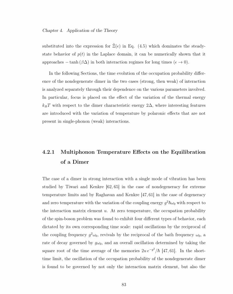
Chapter 4. Application of the Theory
substituted into the expression for Ξ(ε) in Eq. (4.5) which dominates the steady-
state behavior of p(t) in the Laplace domain, it can be numerically shown that it
approaches − tanh (β∆) in both interaction regimes for long times (ε→ 0).
In the following Sections, the time evolution of the occupation probability differ-
ence of the nondegenerate dimer in the two cases (strong, then weak) of interaction
is analyzed separately through their dependence on the various parameters involved.
In particular, focus is placed on the effect of the variation of the thermal energy
kBT with respect to the dimer characteristic energy 2∆, where interesting features
are introduced with the variation of temperature by polaronic effects that are not
present in single-phonon (weak) interactions.
4.2.1 Multiphonon Temperature Effects on the Equilibration
of a Dimer
The case of a dimer in strong interaction with a single mode of vibration has been
studied by Tiwari and Kenkre [62, 65] in the case of nondegeneracy for extreme
temperature limits and by Raghavan and Kenkre [47, 61] in the case of degeneracy
and zero temperature with the variation of the coupling energy g2~ω0 with respect to
the interaction matrix element u. At zero temperature, the occupation probability
of the spin-boson problem was found to exhibit four different types of behavior, each
dictated by its own corresponding time scale: rapid oscillations by the reciprocal of
the coupling frequency g2ω0, revivals by the reciprocal of the bath frequency ω0, a
rate of decay governed by gω0, and an overall oscillation determined by taking the
square root of the time average of the memories 2u e−g2/~ [47, 61]. In the short-
time limit, the oscillation of the occupation probability of the nondegenerate dimer
is found to be governed by not only the interaction matrix element, but also the
83
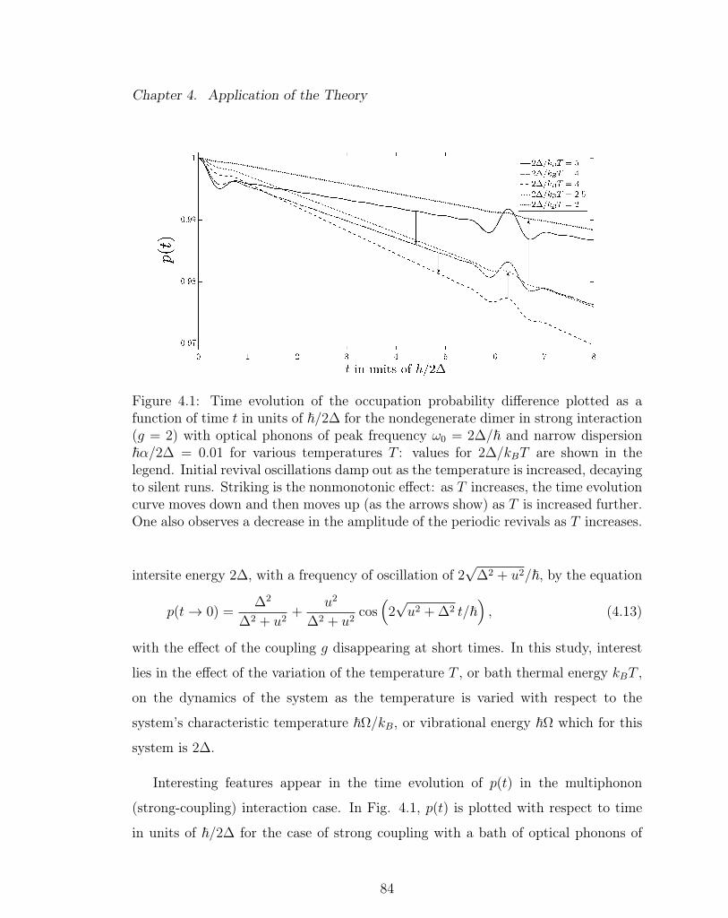
Chapter 4. Application of the Theory
Figure 4.1: Time evolution of the occupation probability difference plotted as afunction of time t in units of ~/2∆ for the nondegenerate dimer in strong interaction(g = 2) with optical phonons of peak frequency ω0 = 2∆/~ and narrow dispersion~α/2∆ = 0.01 for various temperatures T : values for 2∆/kBT are shown in thelegend. Initial revival oscillations damp out as the temperature is increased, decayingto silent runs. Striking is the nonmonotonic effect: as T increases, the time evolutioncurve moves down and then moves up (as the arrows show) as T is increased further.One also observes a decrease in the amplitude of the periodic revivals as T increases.
intersite energy 2∆, with a frequency of oscillation of 2√
∆2 + u2/~, by the equation
p(t→ 0) =∆2
∆2 + u2+
u2
∆2 + u2cos(
2√u2 + ∆2 t/~
), (4.13)
with the effect of the coupling g disappearing at short times. In this study, interest
lies in the effect of the variation of the temperature T , or bath thermal energy kBT ,
on the dynamics of the system as the temperature is varied with respect to the
system’s characteristic temperature ~Ω/kB, or vibrational energy ~Ω which for this
system is 2∆.
Interesting features appear in the time evolution of p(t) in the multiphonon
(strong-coupling) interaction case. In Fig. 4.1, p(t) is plotted with respect to time
in units of ~/2∆ for the case of strong coupling with a bath of optical phonons of
84

Chapter 4. Application of the Theory
peak frequency ω0 = 2∆/~. Both the nonmonotonicity effect brought about by the
associated relaxation rate F21 calculated in Eq. (3.44) and revivals known to exist
in spin-boson systems [61] are noticed at short times. At lower temperatures oscilla-
tions, silent runs, and revivals are evident, as discussed in spin-boson investigations
[61]. As the temperature is increased, the revivals prevalent at vanishing temper-
ature begin to dissipate with increasing T . The nonmonotonicity effect present is
depicted as the arrows show in Fig. 4.1: p(t) decreases as T increases from 1/5 to
1/3 in units of 2∆/kB, and begins to increase as T increases further from 1/3 to 1/2
in those units.
4.2.2 Weak Coupling (Single-Phonon) Temperature Effects
In the case of the single-phonon (weak-coupling) interaction, the behavior of the
occupation probability in one of the two extreme time limits is calculated by following
the Tiwari-Kenkre analysis [62,65]. While the occupation probability difference can
be analytically shown to approach the Boltzmann factor of − tanh (β∆) in the long-
time limit by taking the limit of ε→ 0 of Ξ(ε) in the Laplace domain, the behavior
may be modeled by analyzing the behavior of the sum and difference of the memories.
In the short-time limit, i.e., ω0t 1, the difference in the memories approaches 0
while the sum may be approximated to
F21φS(t) ≈ 4(u2/~2
)cos (2∆t/~) + 2g2ω2
0 coth (β~ω0/2) cos (2∆t/~) . (4.14)
The resulting short-time behavior of the occupation probability difference shows both
a temperature- and interaction-dependent oscillation
p(t→ 0) = 〈p〉+ (1− 〈p〉) cos(
2∆t/~√〈p〉), (4.15)
around the average value 〈p〉 given by
〈p〉 =∆2
∆2 + u2 + (g~ω0)2
2coth (β~ω0/2)
(4.16)
85

Chapter 4. Application of the Theory
Figure 4.2: The time dependence of the occupation probability difference for thenondegenerate dimer with energy 2∆ in weak interaction (g = 0.02) with opticalphonons of peak frequency ω0 = 2∆/~ and dispersion ~α/2∆ = 0.1 for varying tem-peratures T , i.e., for various values of 2∆/kBT . As T is increased, the occupationprobability difference approaches the corresponding equilibrium value faster, with ahigher number of oscillations about the equilibrium value as it approaches equilib-rium. The equilibrium value goes to zero for higher temperatures. No revivals ornonmonotonicity are seen in the time evolution for this weak coupling case.
If there is no interaction with the bath, i.e., g = 0, 〈p〉 reduces to the value given
earlier in ref. [62] and in Eq. (4.13) obtained for an isolated nondegenerate dimer,
i.e., 〈p〉 = ∆2/(∆2 + u2). As the temperature increases, the shifted equilibrium
position approaches zero, while the frequency of oscillation between the two states in
the occupation probability difference at short times becomes infinite. Fig. 4.2 shows
the time evolution of the occupation probability difference between the two dimer
states for various temperatures. As the temperature is increased from zero there is
an increase in the oscillations about the equilibrium value which rises from −1 to
zero with increasing temperature.
86

Chapter 4. Application of the Theory
4.3 Charge in a 1-d Crystal Under a Strong Electric
Field
In this Section, the motion of a charged particle of charge q, in interaction with a
thermal reservoir is studied as the charge moves along the N sites of a 1-dimensional
crystal of lattice constant a under the influence of a strong applied electric field E.
The charge moves in the direction of the applied electric field and the lattice is taken
to exhibit only nearest-neighbor transitions due to the interaction with the bath.
The Hamiltonian describing such an interaction is
H =∑M
EM |M〉〈M |+ u∑M
(|M〉〈M + 1|+ |M + 1〉〈M |)
+∑q
~ωq(b†qbq +
1
2
)+ V , (4.17)
where the |M〉’s are Stark ladder states produced by the action of a strong electric
field acting on the particle and are known to be localized around the sites of the
crystal [66, 67]. Here EM = qEaM is the energy of the particle at site M , u is the
inter-site matrix element between sites, ωq is the frequency the phonon with wave
vector q, the operators bq and b†q create and destroy a phonon with wave vector
q, respectively, and V describes the interaction between the bath of phonons and
particle, as discussed in Chapter 3.
This system which is comprised of an infinite state-space (−∞ < M <∞), has no
lower energy bound, and never approaches thermal equilibrium. It is distinguishable
from its counterparts (the nondegenerate dimer and harmonic oscillator) in that it
exhibits “an approach to steady state” description. This approach to the steady state
is characterized by the evolution of the motion of the charged particle, mainly by
the velocity of the charged particle from the coherent limit at short times to the
incoherent limit in the steady state. In a recent analysis [23] of the dynamics of
such a system, Eq. (4.2) was used to calculate the dependence of the velocity on
87

Chapter 4. Application of the Theory
the microscopic memories φ±(t), suppressing for simplicity the multiplicative factor
of the lattice constant a. The relation found for the velocity was that of the time
integral of the difference in the memories,
v(t) =d〈M(t)〉
dt=
∫ t
0
dsκφD(s). (4.18)
where the φ’s used in the analysis of ref. [23] were of phenomenological form. In this
Section, the derived memories from microscopically specified interactions are used
to analyze the temperature effects on the dynamics of a charged particle as it moves
along a 1-dimensional crystal through the associated time dependent observable, the
particle average velocity, for the two interaction strength regimes considered in this
study.
The system contributed components to the Hamiltonian describing a charged
particle moving along the N sites of a 1-dimensional lattice in interaction with a
bath are
HS =∑M
EM |M〉〈M |,
VS =1√N
∑M
(|M〉〈M + 1|+ |M + 1〉〈M |) , (4.19)
in the weak interaction case as described by the Hamiltonian in Eq. (3.13) and
HS =∑M
(EM − 1
N
∑M,q
g2q~ωq
)|M〉〈M |,
VS,1 =1√N
∑M
|M〉 ˜〈M + 1| and VS,2 =1√N
∑M
˜|M + 1〉〈M |, (4.20)
in the strong interaction case, after transformation, as described by the Hamiltonian
in Eq. (3.15). Here the system component to the shifting operator S which trans-
forms the bare operators in the polaronic transformation to their dressed components
is NS = 1N
∑M |M〉〈M |. The tildes denote shifted operators which may be described
in terms of the bare system and bath operators as |M〉 = |M〉e1√N
∑q gq(bq−b
†q). The
88

Chapter 4. Application of the Theory
system interaction matrix element contribution to the memories in both interaction
cases,∑
j |〈M |VS,j|N〉|2 in the strong coupling case and |〈M |VS|N〉|2 in the weak,
yield (δN,M−1 + δN,M+1). When substituted into the memories of Eqs. (3.4) and
summed over in the GME of Eq. (2.9), the result is Eq. (4.2) with the microscopic
memories κφ±(t) describing the energetically upward and downward transitions.
In taking the bath to be that of phonons with a frequency peaked at ω0 and with
disorder α, the term incorporating the number of sites is absorbed into the coupling
constant, i.e.,∑
qgqN→ g and the microscopic memories, W±(t) = Γφ±(t), obtained
in this study for the interaction with a single mode of vibration (Eqs. (3.41) and
(3.42)) in the two interaction regimes are used in this Section with Ω = E/~ and
Γ = κ, to investigate the approach to equilibrium of the charged particle through
the time evolution of its velocity.
The difference in the memories, κφD(t) = κφ−(t)− κφ+(t) has the form
κφD(t) = 8u2
~2e−g
2 coth(β~ω02 )
∞∑`=1
I`
[g2csch
(β~ω0
2
)]sinh
(`β~ω0
2
)× sin (`ω0t) sin (Et/~) e−αt, (4.21)
in the multiphonon (strong-coupling) case, which when time-integrated yields the
relation for the velocity
v(t) = 4u2
~2e−g
2 coth(β~ω02 )
×∞∑`=1
I`
[g2csch
(β~ω0
2
)]sinh
(`β~ω0
2
)× [f`,−(ω0, t)− f`,−(ω0, 0)− f`,+(ω0, t) + f`,+(ω0, 0)] , (4.22)
where
f`,±(ω0, t) = e−αt(`ω0 ± E/~) sin (`ω0t± E/~t)− α cos (`ω0t± E/~t)
α2 + (`ω0 ± E/~)2 , (4.23)
89
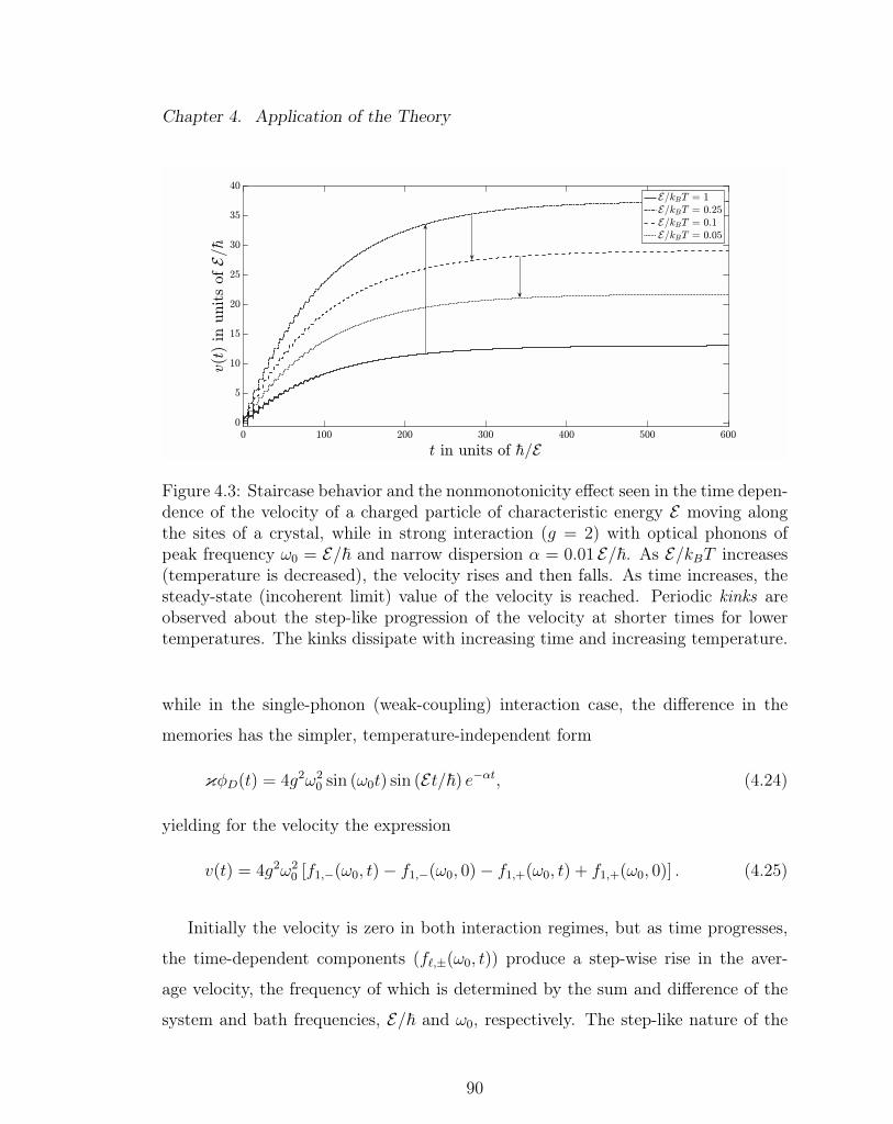
Chapter 4. Application of the Theory
Figure 4.3: Staircase behavior and the nonmonotonicity effect seen in the time depen-dence of the velocity of a charged particle of characteristic energy E moving alongthe sites of a crystal, while in strong interaction (g = 2) with optical phonons ofpeak frequency ω0 = E/~ and narrow dispersion α = 0.01 E/~. As E/kBT increases(temperature is decreased), the velocity rises and then falls. As time increases, thesteady-state (incoherent limit) value of the velocity is reached. Periodic kinks areobserved about the step-like progression of the velocity at shorter times for lowertemperatures. The kinks dissipate with increasing time and increasing temperature.
while in the single-phonon (weak-coupling) interaction case, the difference in the
memories has the simpler, temperature-independent form
κφD(t) = 4g2ω20 sin (ω0t) sin (Et/~) e−αt, (4.24)
yielding for the velocity the expression
v(t) = 4g2ω20 [f1,−(ω0, t)− f1,−(ω0, 0)− f1,+(ω0, t) + f1,+(ω0, 0)] . (4.25)
Initially the velocity is zero in both interaction regimes, but as time progresses,
the time-dependent components (f`,±(ω0, t)) produce a step-wise rise in the aver-
age velocity, the frequency of which is determined by the sum and difference of the
system and bath frequencies, E/~ and ω0, respectively. The step-like nature of the
90
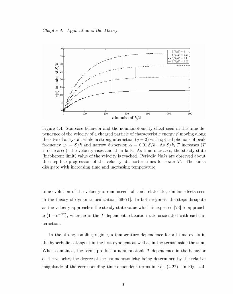
Chapter 4. Application of the Theory
Figure 4.4: Staircase behavior and the nonmonotonicity effect seen in the time de-pendence of the velocity of a charged particle of characteristic energy E moving alongthe sites of a crystal, while in strong interaction (g = 2) with optical phonons of peakfrequency ω0 = E/~ and narrow dispersion α = 0.01 E/~. As E/kBT increases (Tis decreased), the velocity rises and then falls. As time increases, the steady-state(incoherent limit) value of the velocity is reached. Periodic kinks are observed aboutthe step-like progression of the velocity at shorter times for lower T . The kinksdissipate with increasing time and increasing temperature.
time-evolution of the velocity is reminiscent of, and related to, similar effects seen
in the theory of dynamic localization [69–71]. In both regimes, the steps dissipate
as the velocity approaches the steady-state value which is expected [23] to approach
κ(1− e−βE
), where κ is the T -dependent relaxation rate associated with each in-
teraction.
In the strong-coupling regime, a temperature dependence for all time exists in
the hyperbolic cotangent in the first exponent as well as in the terms inside the sum.
When combined, the terms produce a nonmonotonic T dependence in the behavior
of the velocity, the degree of the nonmonotonicity being determined by the relative
magnitude of the corresponding time-dependent terms in Eq. (4.22). In Fig. 4.4,
91

Chapter 4. Application of the Theory
this nonmonotonic effect can be seen in the approach to steady state of the velocity
with time. In the multiphonon (strong-coupling) case, the velocity approaches
vss =2u2
~2e−g
2 coth(β~ω02 )
∞∑`=−∞
I`[2g2n (ω0)
]×∞∑k=0
g2k
k!
[α
α2 + [(k + `)ω0 − E/~]2− α
α2 + [(k + `)ω0 + E/~]2
](4.26)
wherein the expression can be shown to have a direct dependence on the associated
relaxation rate (Eq. (3.44) with Ω = E/~) and approaches the expected steady-state
value.
The steady-state value of the velocity in the single-phonon (weak-coupling) case,
on the other hand, has a temperature independent form
vss = 4g2ω20
[α
α2 + (ω0 − E/~)2 −α
α2 + (ω0 + E/~)2
]. (4.27)
When written in terms of its associated relaxation rate (Eq. (3.45 with Ω = E/~),
this can be easily shown to reproduce the expected steady-state value of κ(1− e−βE
).
One of the factors responsible for the temperature independence evident in Eq. (4.27)
is that there is only a single phonon band involved. We therefore investigated the case
that two phonon bands are involved, following the description detailed in ref. [12].
The result is displayed in Fig. 4.5. The inset shows the T independence arising from
the single phonon band. The main figure, however, displays the expected dependence
on T . The two phonon bands are peaked at frequency ω1 and ω2, respectively, and
are of narrow width. The resulting memories are of the form
κφ±(t) = 2g21g
22~2ω2
1ω22n(ω1)n(ω2)e−αt
×eβ~(ω1+ω2) cos [(ω1 + ω2 ± E/~) t] + cos [(ω1 + ω2 ∓ E/~) t]
+ eβ~ω1 cos [(ω1 − ω2 ± E/~) t] + eβ~ω2 cos [(ω1 − ω2 ∓ E/~) t],
(4.28)
92
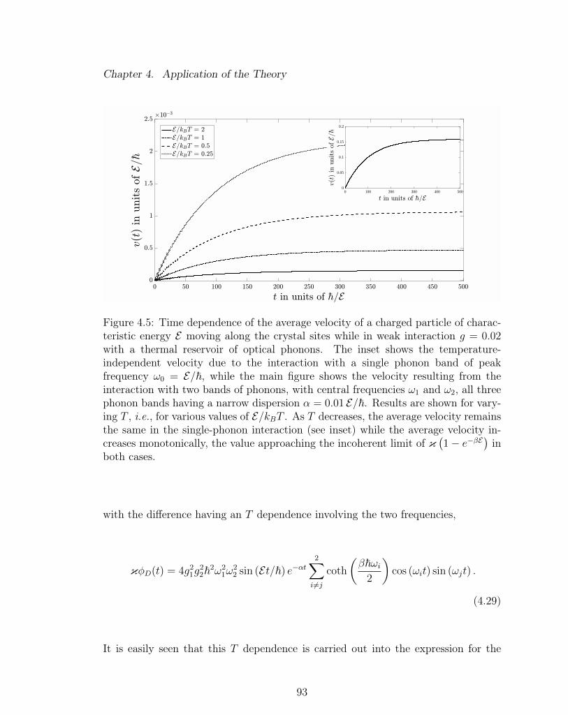
Chapter 4. Application of the Theory
Figure 4.5: Time dependence of the average velocity of a charged particle of charac-teristic energy E moving along the crystal sites while in weak interaction g = 0.02with a thermal reservoir of optical phonons. The inset shows the temperature-independent velocity due to the interaction with a single phonon band of peakfrequency ω0 = E/~, while the main figure shows the velocity resulting from theinteraction with two bands of phonons, with central frequencies ω1 and ω2, all threephonon bands having a narrow dispersion α = 0.01 E/~. Results are shown for vary-ing T , i.e., for various values of E/kBT . As T decreases, the average velocity remainsthe same in the single-phonon interaction (see inset) while the average velocity in-creases monotonically, the value approaching the incoherent limit of κ
(1− e−βE
)in
both cases.
with the difference having an T dependence involving the two frequencies,
κφD(t) = 4g21g
22~2ω2
1ω22 sin (Et/~) e−αt
2∑i 6=j
coth
(β~ωi
2
)cos (ωit) sin (ωjt) .
(4.29)
It is easily seen that this T dependence is carried out into the expression for the
93

Chapter 4. Application of the Theory
velocity
v(t) = g21g
22~2ω2
1ω22
1∑k=0
[coth
(β~ω2
2
)+ (−1)k coth
(β~ω1
2
)]
×
f1,− (xk, t)− f1,− (xk, 0)− f1,+ (xk, t) + f1,+ (xk, 0)
,
(4.30)
where f`,± (xk, t) is as in Eq. (4.23) with xk = ω1 + (−1)kω2. The temperature
dependence present in the expression for the velocity in this weak interaction with
two phonons displays a monotonic behavior with T (see Fig. 4.5).
4.4 Energy of a Relaxing Molecule Modeled as a
Harmonic Oscillator
The recent generalization of Kenkre and Chase in ref. [23] of the Montroll-Shuler
equation (MSE) [6] evident in Eq. (4.3) has led to the result that the molecular
energy E(t) = ~Ω∑
M (M + 1/2)PM(t) obeys
E(t) = E(0)η(t) + Eth
∫ t
0
ds ξ(t− s) [1− η(s)] (4.31)
where E(0) is the initial energy of the system, Eth = ~Ω2
coth(β~Ω
2
)is its thermal or
steady-state value, and η(t) and ξ(t) are the Laplace inverses of
η(ε) =1
ε+ κφD(ε)and ξ(ε) =
φS(ε)
φD(ε)tanh
(β~Ω
2
), (4.32)
respectively. Eq. (4.31) extends the traditional (incoherent) result of
E(t) = E(0)e−κ(1−e−β~Ω)t + Eth
[1− e−κ(1−e−β~Ω)t
](4.33)
to arbitrary coherence. That result is recovered from Eq. (4.31) in the Markoffian
limit that φ(ε)’s are replaced by the corresponding φ(0)’s. In this Section, the forms
94
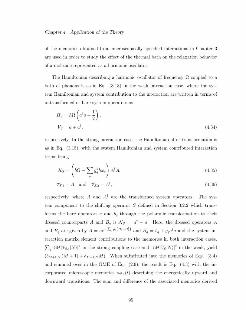
Chapter 4. Application of the Theory
of the memories obtained from microscopically specified interactions in Chapter 3
are used in order to study the effect of the thermal bath on the relaxation behavior
of a molecule represented as a harmonic oscillator.
The Hamiltonian describing a harmonic oscillator of frequency Ω coupled to a
bath of phonons is as in Eq. (3.13) in the weak interaction case, where the sys-
tem Hamiltonian and system contribution to the interaction are written in terms of
untransformed or bare system operators as
HS = ~Ω
(a†a+
1
2
),
VS = a+ a†, (4.34)
respectively. In the strong interaction case, the Hamiltonian after transformation is
as in Eq. (3.15), with the system Hamiltonian and system contributed interaction
terms being
HS =
(~Ω−
∑q
g2q~ωq
)A†A, (4.35)
VS,1 = A and VS,2 = A†, (4.36)
respectively, where A and A† are the transformed system operators. The sys-
tem component to the shifting operator S defined in Section 3.2.2 which trans-
forms the bare operators a and bq through the polaronic transformation to their
dressed counterparts A and Bq is NS = a† − a. Here, the dressed operators A
and Bq are given by A = ae−∑q gq(Bq−B
†q) and Bq = bq + gqa
†a and the system in-
teraction matrix element contributions to the memories in both interaction cases,∑j |〈M |VS,j|N〉|2 in the strong coupling case and |〈M |VS|N〉|2 in the weak, yield
(δM+1,N (M + 1) + δM−1,NM). When substituted into the memories of Eqs. (3.4)
and summed over in the GME of Eq. (2.9), the result is Eq. (4.3) with the in-
corporated microscopic memories κφ±(t) describing the energetically upward and
downward transitions. The sum and difference of the associated memories derived
95
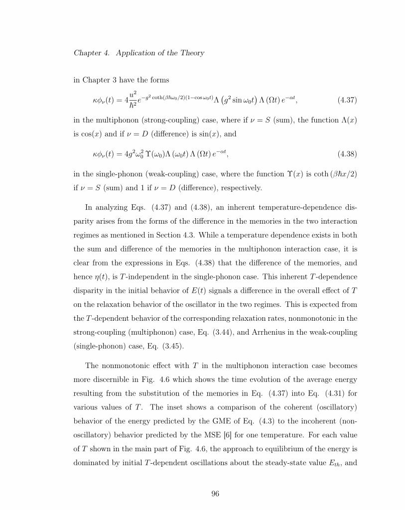
Chapter 4. Application of the Theory
in Chapter 3 have the forms
κφν(t) = 4u2
~2e−g
2 coth(β~ω0/2)(1−cosω0t)Λ(g2 sinω0t
)Λ (Ωt) e−αt, (4.37)
in the multiphonon (strong-coupling) case, where if ν = S (sum), the function Λ(x)
is cos(x) and if ν = D (difference) is sin(x), and
κφν(t) = 4g2ω20 Υ(ω0)Λ (ω0t) Λ (Ωt) e−αt, (4.38)
in the single-phonon (weak-coupling) case, where the function Υ(x) is coth (β~x/2)
if ν = S (sum) and 1 if ν = D (difference), respectively.
In analyzing Eqs. (4.37) and (4.38), an inherent temperature-dependence dis-
parity arises from the forms of the difference in the memories in the two interaction
regimes as mentioned in Section 4.3. While a temperature dependence exists in both
the sum and difference of the memories in the multiphonon interaction case, it is
clear from the expressions in Eqs. (4.38) that the difference of the memories, and
hence η(t), is T -independent in the single-phonon case. This inherent T -dependence
disparity in the initial behavior of E(t) signals a difference in the overall effect of T
on the relaxation behavior of the oscillator in the two regimes. This is expected from
the T -dependent behavior of the corresponding relaxation rates, nonmonotonic in the
strong-coupling (multiphonon) case, Eq. (3.44), and Arrhenius in the weak-coupling
(single-phonon) case, Eq. (3.45).
The nonmonotonic effect with T in the multiphonon interaction case becomes
more discernible in Fig. 4.6 which shows the time evolution of the average energy
resulting from the substitution of the memories in Eq. (4.37) into Eq. (4.31) for
various values of T . The inset shows a comparison of the coherent (oscillatory)
behavior of the energy predicted by the GME of Eq. (4.3) to the incoherent (non-
oscillatory) behavior predicted by the MSE [6] for one temperature. For each value
of T shown in the main part of Fig. 4.6, the approach to equilibrium of the energy is
dominated by initial T -dependent oscillations about the steady-state value Eth, and
96

Chapter 4. Application of the Theory
Figure 4.6: Nonmonotonic temperature dependence of the molecular energy for thestrong-coupling case shown via the time evolution of the energy E(t) scaled to itsthermal value Eth. Here the molecular frequency Ω equals the peak frequency of thebath phonons ω0, g = 2, and α/ω0 = 0.01. We plot E(t) for varying T/T0 whereT0 = ~ω0/kB (see legend). A nonmonotonic T -dependence is observed as T increases,first a rise and then a drop (see arrows). The inset shows the difference between theincoherent limit (Montroll-Shuler, see text) (dash-dot line) and our GME predictions(solid line) for one representative case, T/T0 = 1.
then dissipating to it. The nonmonotonic T dependence is seen clearly in the rise and
fall of the peak amplitude of the energy as T is increased. As the figure shows, the
peak value of the energy rises initially (from a to b) with increasing T and then falls
(from c to d) as the period of oscillation increases monotonically. This nonmonotonic
behavior may be explained by the temperature dependence of the relaxation rate in
Eq. (3.44).
Another noteworthy feature which is emphasized particularly at low tempera-
tures is the existence of periodic kinks observed along the main curve of E(t), the
kink amplitudes dissipating with the progression of time (see Fig. 4.9). As the tem-
perature is increased the time interval over which the kinks are visible is decreased.
97

Chapter 4. Application of the Theory
These kinks result from the competition between the periods inside each of the two
cosines in the memories of Eqs. (4.37) and are related to the revivals which are
known to exist in spin-boson systems [61, 72]. An explanation for the kinks arises
when analyzing the zero temperature behavior of the difference in the memories in
the multiphonon regime which may be written in its series representation as
κφD(t) = 4u2
~2e−g
2∞∑m=0
g2m
m!sin (mω0t) sin (Ωt) e−αt. (4.39)
As m is increased, the sign and magnitude of the amplitude of the product of the two
sines in the sum changes more rapidly with time. When all these terms are added
together, the small changes in the amplitude which form the kinks start to negate
each other at longer times, allowing for smooth overall oscillations in the behavior
of E(t). As the temperature is turned on, the lifetime of the interplay between the
two amplitudes is decreased, allowing for a smoothing over in the curve defined by
the energy.
In the Laplace domain Eqs. (4.37) and Eqs. (4.38) have the forms, respectively,
of
κφν(ε) = 4u2
~2e−g
2 coth(β~ω0/2)
∞∑`=−∞
I`[g2csch
(β~ω0
2
)]e`
β~ω02 (ε+ α)χ` (ε)[
(ε+ α)2 + (`ω0 + Ω)2] [(ε+ α)2 + (`ω0 − Ω)2] , (4.40)
and
κφν(ε) = 4g2ω20 Υ(ω0)
(ε+ α)χ1(ε)[(ε+ α)2 + (ω0 + Ω)2] [(ε+ α)2 + (ω0 − Ω)2] , (4.41)
where if ν = S, the function χ`(ε) is Ω2 + `2ω20 + (ε+ α)2 and if ν = D it is 2`ω0Ω. It
can be shown, either numerically in the multiphonon case or analytically in the single-
phonon case, that in the limit ε→ 0, the ratio of the Laplace transform of the sum
and difference of these microscopically derived memories approaches coth (β~Ω/2).
98

Chapter 4. Application of the Theory
Figure 4.7: Absence of interesting results such as nonmonotonicity for weak-coupling(single-phonon interactions). The time evolution of the average energy of a harmonicoscillator of characteristic frequency Ω in weak interaction (g = 0.02) with opticalphonons of peak frequency ω0 = Ω and narrow dispersion α/ω0 = 0.01 is plottedwith respect to time t, for varying T . As T is increased, the average energy initiallyrises above the incoherent limit value, with oscillations decaying faster to Eth. Thefrequency of oscillation remains the same for all T , while the amplitude shows adirect T dependence, increasing with increasing T .
In the case of weak interaction, similar relaxation behavior of the energy to that
of the case of strong interaction is obtained, with initial oscillations about, and
dissipation to, the steady-state value Eth at long times with temperature-dependent
amplitudes (see Fig. 4.7). The energy in this case has the analytic form of
E(t) =
[E(0)− Eth
tanh(β~Ω
2
)tanh
(β~ω0
2
)Ω2 + ω20 + α2
2ω0Ω
]η(t)
+ Ethtanh
(β~Ω
2
)tanh
(β~ω0
2
)Ω2 + ω20 + α2
2ω0Ω. (4.42)
99

Chapter 4. Application of the Theory
where
η(t) = e−αtL−1
[ε2 + (ω0 + Ω)2] [ε2 + (ω0 − Ω)2][
ε2 + (ω0 + Ω)2] [ε2 + (ω0 − Ω)2] (ε− α) + 8g2ω30Ωε
.
(4.43)
While no general analytic solution exists for η(t), it is evident that it is temperature
independent in the single-phonon interaction case, and that the behavior of η(t) is
of decaying oscillatory form as expected. The decay introduced in the memories
through disorder becomes the explicit reason for the decay of the energy of the
oscillator in this regime, while the amplitude of oscillation in the energy is determined
by the temperature-dependent term ξ(t) which is a delta function in time with and
amplitude equal to the term multiplying Eth in Eq. (4.42).
4.4.1 Introduction of a Relaxation Memory and an Effective
Rate
As seen in the previous Sections, the relaxation rate can be obtained through the
Fourier transform of the microscopically derived bath correlation function B(t) eval-
uated at the oscillator frequency. In this Section, we develop an approach in terms
of a relaxation memory and an effective rate. The incoherent result [6], Eq. (2.7),
may be rewritten as
E(t)− EthE(0)− Eth
= e−κ(1−e−β~Ω)t (4.44)
to emphasize that the effective rate of relaxation is κ(1− e−β~Ω
). Although the
generalization in ref. [23] reflected in Eq. (4.31) results in a non-exponential time-
dependence of the left hand side of Eq. (4.44), its Laplace transform can always be
expressed as
E(ε)− Eth/εE(0)− Eth
=1
ε+ ζ(ε), (4.45)
100

Chapter 4. Application of the Theory
through the introduction of the Laplace transform of a relaxation memory ζ(t). In
the incoherent Master equation approximation, ζ(t) is κ(1− e−β~Ω
)δ(t), while in
the general case, ζ(t) describes coherent oscillations present in the exact result of
E(t) obtained from Eq. (4.31). The memory is found through the corresponding
relation of the energy in Eq. (4.31) in the Laplace domain as
ζ(ε) =ε[E(0)− Ethξ(ε)
][1− εη(ε)]
E(0)− Eth −[E(0)− Ethξ(ε)
][1− εη(ε)]
. (4.46)
We now provide a formula for an effective rate of relaxation in the presence of
non-exponential time evolution of the energy E(t) that can take into account the
consequences of all non-exponential features including oscillations. We define it from
Eq. (4.46) by applying the Markoffian approximation to ζ(t). This means putting
the Laplace variable equal to zero in the right hand side of Eq (4.46), and yields
ζ(0) =1∫∞
0E(t)−EthE(0)−Eth
dt(4.47)
If the evolution were totally incoherent (exponential time-dependence), there
would be no oscillations and this effective rate would equal the incoherent rate
κ(1− e−β~Ω
). But if there are oscillations due to coherence, Eq. (4.47) would take
them into account as they would enter the effective rate through the integration of
the oscillations in the denominator of its right hand side. Eq. (4.47) is a prescription
that can be used in this fashion on experimental observations of the energy time
dependence. An interesting result emerges when we use it on the numerical solutions
we have obtained above. Using the microscopic memories derived in Eqs. (2.27), the
behavior of the Markoffian rate ζ(0) is plotted with respect to temperature in Fig.
4.8 for the strong interaction case as compared to the incoherent result of Montroll
and Shuler [6]. The plot shows multiple oscillations with increasing T for the scaled
effective rate in the strong-coupling (multiphonon) case, while exhibiting a simple
and expected monotonic decay with T in the weak-coupling (single-phonon) case.
101

Chapter 4. Application of the Theory
Figure 4.8: Multiple oscillations (solid line) in the temperature dependence of thenormalized effective rate of change of the energy, ζT (0)/ζT=0(0) (see text) for thestrong-coupling case. Parameter values are g = 2, ω0 = Ω, and α/Ω = 0.01. Forcomparison, we display the same rate as calculated from the Montroll-Shuler analysisin ref. [6] which shows no oscillations and is, indeed, 1− e−~Ω/kBT .
By contrast, the original incoherent Master equation of ref. [6] results in no oscilla-
tions (dashed curve) as the ratio ζT (0)/ζT=0(0) in the Montroll-Shuler curve is simply
1− e−~Ω/kBT , with the Montroll-Shuler rate κ being equivalent to the T -independent
term ζT=0(0). An overall nonmonotonic T dependence exists in the strong interaction
regime, where the increasing or decreasing behavior is determined by the T interval
in which observations are made.
4.4.2 The Half-Markoffian Approximation: Developing an In-
terpolation Formula
In this Section, on the basis of the half-Markoffian approximation discussed in refs.
[64, 73], we develop a useful interpolation formula to describe the time evolution of
102

Chapter 4. Application of the Theory
the energy. It is found to be exact at very short and very long times, and to provide
an approximate description at intermediate times. The half-Markoffian approxima-
tion is defined by taking an expression which is a convolution of two functions and
approximating it by a convolutionless expression as∫ t
0
ds f(t− s)g(s) ≈ g(t)
∫ t
0
ds f(s). (4.48)
We begin by converting Eq. (4.31) to the integro-differential equation
dE(t)
dt+
∫ t
0
dt′ κφD(t− t′)E(t′) = Eth tanh
(β~Ω
2
)∫ t
0
dt′ κφS(t′), (4.49)
and simplifying it further to the form
dE(t)
dt+
∫ t
0
dt′ κφD(t− t′)E(t′) =~Ω
2
∫ t
0
dt′ κφS(t′). (4.50)
Eq. (4.48) is applied to the second term in Eq. (4.50) to yield
E(t) =~Ω
2+
[E(0)− ~Ω
2
]e−
∫ t0 dt′ID(t′) + ~Ω
∫ t
0
dt′I+(t′)e−∫ tt′ dsID(s), (4.51)
where Iν(t) =∫ t
0dt′κφν(t
′).
The exponential decay of the second term of the energy in Eq. (4.51) which is de-
pendent on the difference in the memories, κφD(t), parallels the inherent exponential
decay of η(t) in Eq. (4.31), starting from a finite value and decaying to zero over time.
The first term describes the zero temperature result for the energy in the steady-
state, which when combined with the third term, reveals a temperature dependence,
which in the long time limit approaches the steady-state value of the energy Eth.
When the Markoffian approximation is applied and Iν(t→∞) = κ(1± e−β~Ω
), the
‘+’ corresponding to ν = S and the ‘−’ to ν = D, the incoherent Montroll-Shuler [6]
or Bethe-Teller result [13] is reproduced from Eq. (4.51):
E(t) = E(0)e−κ(1−e−β~Ω)t + Eth
[1− e−κ(1−e−β~Ω)t
]. (4.52)
Substitution of Eq. (4.37) and Eqs. (4.37) into Eq. (4.51) shows that the kinks
visible for low temperatures and short times in the form of the exact solution indeed
103

Chapter 4. Application of the Theory
Figure 4.9: Interpolation formula developed as Eq. (4.51) on the basis of the half-Markoffian approximation (see text) showing excellent agreement at extreme (bothshort and long) times but considerable departures at intermediate times. The energy,scaled to its thermal value, is plotted for very low T for g = 2, ω0 = Ω + α/2,and α/Ω = 0.02. The kinks visible at short times (left panel) and equilibrationto the steady-state result (Bethe-Teller) of the energy (middle panel) are faithfullyreproduced by our interpolation formula. The full evolution over the three regimesof time are depicted in right panel.
arise from the behavior of the difference in the memories, at least at short times.
Fig. 4.9 shows the half-Markoffian approximation in comparison to the exact and
Bethe-Teller results. An excellent agreement is seen at both short and long times
(left and middle panels) or our interpolation formula with the exact result, but fails
to predict the intermediate behavior (right panel) accurately.
4.5 Concluding Remarks
The investigation of the relaxation to equilibrium of three simple quantum systems
has uncovered some interesting and perhaps unexpected results when the system-
104

Chapter 4. Application of the Theory
reservoir interaction is strong. One of the interesting effects is a nonmonotonic
variation of the observable associated with each system. It is apparent in the oc-
cupation probability difference for the simple nonresonant dimer (first system); in
the temperature dependence of the steady-state value of the velocity of the charged
particle moving across the sites of a crystal under the influence of a strong electric
field (second system); and in the temperature variation of the energy of the molec-
ular oscillator (third system), where the effective rate of change of the energy and
initial peak amplitude of the energy are shown to exhibit a nonmonotonic rise with
temperature. This nonmonotonic effect is seen only for strong coupling (effectively
multiphonon interactions) and has been shown explicitly that it does not arise for
weak-coupling (single-phonon interactions).
The evaluation of the occupation probability difference of the nondegenerate
dimer, the steady-state expression of the velocity of the charged particle, and the
generalization of the well-known Bethe-Teller result, when combined with the micro-
scopically calculated memories have afforded insight into the effects of the interaction
strength of the system with the thermal reservoir. The generalization of the Montroll-
Shuler equation into the GME introduced in ref. [23] and calculated explicitly as
we have done in the present study in microscopic interactions leads to an interesting
result. Multiple oscillations with respect to temperature appear in the effective rate
we have defined. It is obvious from the study presented here that bath dynamics
result not only in expected consequences of the strength of the interaction but also
in (perhaps) counter-intuitive oscillatory behavior as one varies the temperature.
A useful byproduct of the analysis is the half-Markoffian approximation that has
been developed in Section 4.4. Derived from the integro-differential equation for the
energy in Eq. (4.50), it allows the user to avoid convolutions. It is shown to be able
to predict rather well the extreme, that is short- and long-time, relaxation behavior
of the molecular oscillator, although it does not provide an accurate prescription for
105

Chapter 4. Application of the Theory
intermediate times. Its advantage lies in eliminating the necessity for excursions into
the Laplace domain.
The peculiar temperature variation of the relaxation of the last system analyzed
here (Section 4.4) may be related to observations reported by Fayer and collaborators
[5, 16] (see discussion in Chapter 2). The experimental report given a couple of
decades ago, concerned W(CO)6 dissolved in CHCl3 and provided an explanation
of an “inverted” T -dependence of relaxation on the basis of assumed properties of
the liquid phonon density of the solvent. It is possible that the analysis presented
here in Fig. 4.8 might provide an alternate explanation on the basis of the more
straight-forward polaronic features of the interaction assumed in this study.
106

Chapter 5
Single-Mode Approximation and
Connection to Hypergeometric
Functions
In this Chapter, exact calculations for the memories and rates are presented on the
basis of the single-mode approximation. It is particularly suitable for the interaction
with a bath of optical phonons of peak frequency ω and narrow bandwidth [18].
A proof of strict agreement with the detailed balance condition in the case of no
disorder is outlined through the use of the Dirac comb properties. The introduction
of disorder as a means to remedy the unphysical results of infinite rates [18,63,74–76],
which was briefly touched upon in Chapter 3, is discussed in more detail. While the
rates resulting from such a case may be finite through the introduction of decay
to the memories, a deviation from detailed balance arises in their ratios for low
temperatures. A remedy considered in restoring detailed balance for all temperature
in this case is introduced via the coarsening of the spectral function in ω-space
through the introduction of rectangular functions.
107

Chapter 5. Single-Mode Approximation
A connection of the spectral function, and hence the rates, is made to a spe-
cial case of the generalized hypergeometric function which exhibits nonmonotonic
behavior with the variation of its variables. An investigation of the 2F2 function is
presented as a means to understand the relaxation behavior of an arbitrary nonde-
generate system in interaction with a bath described by the microscopic prescriptions
presented in this dissertation and in previous literature [18, 47, 48, 58, 60–62]. The
spectral function and rates are introduced in terms of I-Bessel function propagators
and multiplicative amplitude-determining terms in order to obtain expressions for
the critical temperature at which the rates start decreasing with temperature.
5.1 Proof of Strict Detailed Balance
In much of the previous literature [48,58,60] used as guidance in present calculations,
the strong interaction of a system with a single mode of vibration has been analyzed
with some extensions made later to approximate and exact forms of interactions with
optical phonon bands [47, 58, 61]. The system particular to all of the calculations
present in the literature is that of the spin-boson [44,47,61] or nondegenerate dimer
[62].
As considered in this study, the bath correlation function describing the strong
interaction with a single mode of vibration, where the phonons are characterized by
a peak frequency ω, is as in Eq. (3.21)
B(t) = u2e−g2 coth(β~ω2 )eg
2[coth(β~ω2 ) cosωt+i sinωt], (5.1)
and the corresponding memories are written as
W±(t) = 2u2
~2e−g
2 coth(β~ω2 )(1−cosωt) cos(g2 sinωt± Ωt
), (5.2)
where Ω is the characteristic frequency of the nondegenerate system involved, the +
and − signs indicating energetically upward and downward transitions, respectively.
108

Chapter 5. Single-Mode Approximation
Figure 5.1: The time dependence of the memories corresponding to energeticallyupward and downward transitions for a nondegenerate system with characteristicfrequency Ω in strong interaction (g = 2) with a single mode of vibration of frequencyω = Ω with T = ~ω/kB. The memories are observed to exhibit nondecaying behavior.
The memories in Eqs. (3.39), as mentioned in Section 3.4, never decay to zero,
their time integrals yielding infinite transition rates, a quite unphysical result. This,
as mentioned earlier (see discussion in Chapter 3), is a consequence of the linear
interactions considered in this study, wherein the zero-phonon lines present in the
optical spectra of defects in solids are neither displaced nor broadened [17,55]. How-
ever, it can be shown that despite the unphysical results eventually obtained from
these nondecaying memories the associated spectral function does satisfy the detailed
balance condition of
Y(z) = eβ~zY(−z). (5.3)
109

Chapter 5. Single-Mode Approximation
Proof of Strict Detailed Balance Agreement
In its series representation, Eq. (5.1) may be rewritten as
B(t) = u2e−g2 coth(β~ω2 )
∞∑`=−∞
I`
[g2csch
(β~ω
2
)]e`
β~ω2 ei`ωt, (5.4)
or equivalently as
B(t) = u2e−g2 coth(β~ω2 )
∞∑`=−∞
I`[2g2n(ω)
] ∞∑k=0
g2k
k!ei(`+k)ωt. (5.5)
When Fourier-transformed with the use of the definition of the spectral function in
terms of the bath correlation fuction in Eq. (3.10), the bath spectral function is
found to have the form
Y(z) = 2u2
~2e−g
2 coth(β~ω2 )
×∞∑
`=−∞
I`[2g2n(ω)
] ∞∑k=0
g2k
k!δ (z − Ω− (`+ k)ω) . (5.6)
It is evident from the delta function expression in Eq. (5.6) that it will be zero for
all z’s except for z = Ω + (`+ k)ω, at which values it will be infinite due to the
existence of the weighted delta functions in the sum. As a result, the transition rates
are found to be infinite unless only the magnitude of the terms multiplying each of
the corresponding delta functions is considered. However, detailed balance is still
satisfied by Eq. (5.6).
In order to prove this, let us first define the Dirac comb [77]:
X (a)∞∑k=0
f(k) ≡∞∑k=0
X (k − a) f(k). (5.7)
Beginning with the spectral function expression in Eq. (5.6) and scaling the Dirac
delta function so that its argument is dimensionless, the spectral function may be
110

Chapter 5. Single-Mode Approximation
written in terms of the Dirac comb as
Y(z) =2
ω
(u~
)2
e−g2 coth(β~ω2 )
×∞∑k=0
g2k
k!X(z − Ω
ω− k)I( z−Ω
ω−k)[2g2n(ω)
]. (5.8)
As both the Dirac comb and the I-Bessel functions are even functions, one in its
argument, i.e., X(−x) = X(x), and one in its index, i.e., I`(x) = I−`(x), the
argument in the sum over k in Eq. (5.8) may be rewritten such that the spectral
function takes the form
Y(z) =2
ω
(u~
)2
e−g2 coth(β~ω2 )
×∞∑k=0
g2k
k!X(k − z − Ω
ω
)I(k− z−Ω
ω )[2g2n(ω)
]. (5.9)
The Dirac comb has the property that, when summed over, it can be extracted
from the sum and evaluated at the value at which its argument is equal to zero, i.e.,
∞∑k=0
X (k − a) f(k) ≡X (a)∞∑k=0
f(k). (5.10)
Using the above property, Eq. (5.9) may be rewritten as
Y(z) =2
ω
(u~
)2
e−g2 coth(β~ω2 )X
(z − Ω
ω
) ∞∑k=0
g2k
k!I(k− z−Ω
ω )[2g2n(ω)
]. (5.11)
Here, the identity of the sum over I-Bessel functions of
λ−νIν (λx) =∞∑k=0
[(λ2−1)x
2
]kk!
Ik+ν (x) , (5.12)
where x = 2g2n(ω) and ν = Ω−zω
, is used to rewrite the sum in Eq. (5.11) as
∞∑k=0
g2k
k!I(k− z−Ω
ω )[2g2n(ω)
]= e
β~(z−Ω)2 I( z−Ω
ω )
[g2csch
(β~ω
2
)]. (5.13)
111

Chapter 5. Single-Mode Approximation
Substituting Eq. (5.13) into Eq. (5.11) the expression for the spectral function takes
the form
Y(z) =2
ω
(u~
)2
e−g2 coth(β~ω2 )e
β~(z−Ω)2 X
(z − Ω
ω
)I( z−Ω
ω )
[g2csch
(β~ω
2
)].
(5.14)
When Eq. (5.14) is evaluated at −z it yields
Y(−z) =2
ω
(u~
)2
e−g2 coth(β~ω2 )e−
β~(z+Ω)2
×X(z + Ω
ω
)I( z+Ω
ω )
[g2csch
(β~ω
2
)]. (5.15)
and the ratio of Eqs. (5.14) and (5.15) yields
Y(z)
Y(−z)=
X(z−Ωω
)I( z−Ω
ω )(g2csch
(β~ω
2
))X(z+Ωω
)I( z+Ω
ω )(g2csch
(β~ω
2
)) eβ~z. (5.16)
The only difference between the numerator and denominator in Eq. (5.16) is the
argument of the Dirac comb and the index of the I-Bessel function. The existence
of the Dirac comb limits the values of (z − Ω)/ω to be integer values at which
delta functions exist with their corresponding magnitudes being determined by the
function multiplying them. This, in combination with the sampling property of the
Dirac comb where
X(x)f(x) =∞∑
`=−∞
f(`)δ (x− `) , (5.17)
allows for the equivalence property,
X(z − Ω
ω
)I( z−Ω
ω )
[g2csch
(β~ω
2
)]= X
(z + Ω
ω
)I( z+Ω
ω )
[g2csch
(β~ω
2
)](5.18)
to be used since a sum is taken over all the `’s in the infinite domain. Substituting
Eq. (5.18) into Eq. (5.16) the result of detailed balance, i.e.,
Y(z) = Y(−z)eβ~z, (5.19)
is obtained.
112
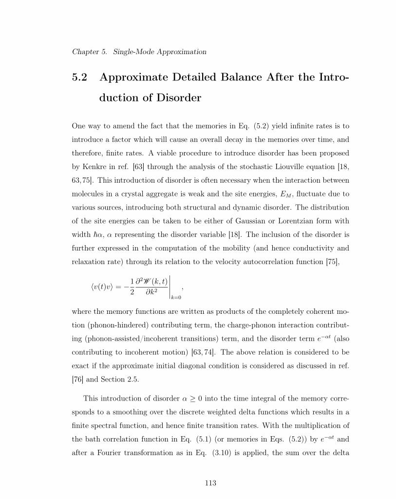
Chapter 5. Single-Mode Approximation
5.2 Approximate Detailed Balance After the Intro-
duction of Disorder
One way to amend the fact that the memories in Eq. (5.2) yield infinite rates is to
introduce a factor which will cause an overall decay in the memories over time, and
therefore, finite rates. A viable procedure to introduce disorder has been proposed
by Kenkre in ref. [63] through the analysis of the stochastic Liouville equation [18,
63,75]. This introduction of disorder is often necessary when the interaction between
molecules in a crystal aggregate is weak and the site energies, EM , fluctuate due to
various sources, introducing both structural and dynamic disorder. The distribution
of the site energies can be taken to be either of Gaussian or Lorentzian form with
width ~α, α representing the disorder variable [18]. The inclusion of the disorder is
further expressed in the computation of the mobility (and hence conductivity and
relaxation rate) through its relation to the velocity autocorrelation function [75],
〈v(t)v〉 = −1
2
∂2W (k, t)
∂k2
∣∣∣∣∣k=0
,
where the memory functions are written as products of the completely coherent mo-
tion (phonon-hindered) contributing term, the charge-phonon interaction contribut-
ing (phonon-assisted/incoherent transitions) term, and the disorder term e−αt (also
contributing to incoherent motion) [63, 74]. The above relation is considered to be
exact if the approximate initial diagonal condition is considered as discussed in ref.
[76] and Section 2.5.
This introduction of disorder α ≥ 0 into the time integral of the memory corre-
sponds to a smoothing over the discrete weighted delta functions which results in a
finite spectral function, and hence finite transition rates. With the multiplication of
the bath correlation function in Eq. (5.1) (or memories in Eqs. (5.2)) by e−αt and
after a Fourier transformation as in Eq. (3.10) is applied, the sum over the delta
113
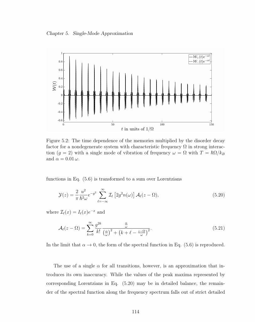
Chapter 5. Single-Mode Approximation
Figure 5.2: The time dependence of the memories multiplied by the disorder decayfactor for a nondegenerate system with characteristic frequency Ω in strong interac-tion (g = 2) with a single mode of vibration of frequency ω = Ω with T = ~Ω/kBand α = 0.01ω.
functions in Eq. (5.6) is transformed to a sum over Lorentzians
Y(z) =2
π
u2
~2ωe−g
2∞∑
`=−∞
I`[2g2n(ω)
]A`(z − Ω), (5.20)
where I`(x) = I`(x)e−x and
A`(z − Ω) =∞∑k=0
g2k
k!
αω(
αω
)2+(k + `− z−Ω
ω
)2 . (5.21)
In the limit that α→ 0, the form of the spectral function in Eq. (5.6) is reproduced.
The use of a single α for all transitions, however, is an approximation that in-
troduces its own inaccuracy. While the values of the peak maxima represented by
corresponding Lorentzians in Eq. (5.20) may be in detailed balance, the remain-
der of the spectral function along the frequency spectrum falls out of strict detailed
114

Chapter 5. Single-Mode Approximation
Figure 5.3: Plots of the spectral function (left panel) and upward (Γ+) and downward(Γ−) transition rates (right panels). The parameter values are g = 2, α = 0.01ω,ω = Ω, and T = ~ω/kB. The spectral function is plotted with respect to thefrequency z in units of ω and the rates are plotted with respect to the temperature Tin units of T0, where T0 = ~ω/kB. Multiple peaks are visible in the spectral function,each peak with a corresponding magnitude, center, and width. Strict agreement withdetailed balance is observed to fail at low temperatures for the case in which the ratesare described by Lorentzians, the effect becoming more dramatic, extending over tohigher temperatures as α/ω increases.
balance. As seen in Fig. 5.3, the corresponding rates
Γ± = 2u2
~2ωe−g
2∞∑
`=−∞
I`[2g2n(ω)
]A`(±Ω), (5.22)
satisfy detailed balance at higher temperatures, but fail to do so for low T .
The remedy in restoring detailed balance for all T lies in coarsening the descrip-
tion in ω-space and considering a rectangular function of narrow width α centered
about each corresponding frequency $ along the spectrum, i.e.,
1
π
α
α2 +$2≈ 1
αrect
($α
)=
1
α
[Θ($ +
α
2
)−Θ
($ − α
2
)], (5.23)
115
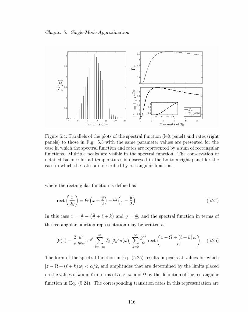
Chapter 5. Single-Mode Approximation
Figure 5.4: Parallels of the plots of the spectral function (left panel) and rates (rightpanels) to those in Fig. 5.3 with the same parameter values are presented for thecase in which the spectral function and rates are represented by a sum of rectangularfunctions. Multiple peaks are visible in the spectral function. The conservation ofdetailed balance for all temperatures is observed in the bottom right panel for thecase in which the rates are described by rectangular functions.
where the rectangular function is defined as
rect
(x
2y
)= Θ
(x+
y
2
)−Θ
(x− y
2
). (5.24)
In this case x = zω−(
Ωω
+ `+ k)and y = α
ω, and the spectral function in terms of
the rectangular function representation may be written as
Y(z) =2
π
u2
~2αe−g
2∞∑
`=−∞
I`[2g2n(ω)
] ∞∑k=0
g2k
k!rect
(z − Ω + (`+ k)ω
α
). (5.25)
The form of the spectral function in Eq. (5.25) results in peaks at values for which
|z − Ω + (`+ k)ω| < α/2, and amplitudes that are determined by the limits placed
on the values of k and ` in terms of α, z, ω, and Ω by the definition of the rectangular
function in Eq. (5.24). The corresponding transition rates in this representation are
116

Chapter 5. Single-Mode Approximation
written as
Γ± = 2u2
~2αe−g
2∞∑
`=−∞
I`[2g2n(ω)
] ∞∑k=0
g2k
k!rect
(±Ω + (`+ k)ω
α
), (5.26)
and detailed balance is restored as seen in Fig. 5.4. In the limit that α/ω → 0, the
forms of the spectral function and rates describing the interaction with phonons of
a single mode of vibration without the introduction of disorder are reproduced.
5.3 Analytic Expression for a Special Case
The form of the spectral function in Eq. (5.20) consists of the sum∑∞
`=−∞ I`(x)A`,
where I`(x) = I`(x)e−x. If A` is equal to unity for all `, then irrespective of the
argument x involved, the sum∑∞
`=−∞ I`(x) is also equal to unity as per the definition
of the Bessel function sum rule. This can be interpreted as the propagator sum of a
moving particle which is unity due to probability conservation. All I`(x) for ` 6= 0
have the same qualitative behavior which is that they start at 0 for x = 0, rise to
some maximum Imax(xc), and then fall to zero. In the case of ` = 0, I0(x) starts at
1 at x = 0 and always falls with no maximum other than at x = 0 (see left panel of
Fig. 5.5).
For the case in which theA`’s are not equal to 1, the slope of the rise or fall of each
of the I`(x)’s is determined by the corresponding weight placed by the associated A`affecting the behavior of the sum, and hence the overall behavior, with respect to the
argument x. While the temperature dependence is only evident in the propagator
terms I`(x), analysis of the behavior of the terms multiplying each I`(x), i.e.,
A`(y) =∞∑k=0
g2k
k!
αω(
αω
)2+(k + `− y
ω
)2 (5.27)
is pertinent in understanding the nonmonotonic effect on the rates in the strong
coupling regime. With this in mind, the functional form of the A`’s will be analyzed
117

Chapter 5. Single-Mode Approximation
Figure 5.5: Plots of I`(x) (left panel) and I`(x)A` (right top panel) with respectto x for ` = 1, 1, 5, ad 100, and A` with respect to `, with parameter values ofg = 2, y = ω, and α = 0.01 Ω. The variation of the nonmonotonic behavior innate inthe sum present in the spectral function and rates with and without the presence ofthe A`’s is shown. The effect that the A`’s have on the dependence of the spectralfunction and rates on x representing the dependence on the temperature, is that iteither amplifies the magnitude of the corresponding I` or drives it to zero. As `reaches some maximum value `max, the terms considered in the sum for ` 6= `max
may be ignored as A` becomes infinitesimally small compared to other componentsin the sum with increasing values of ±`.
in this Section as a function of ` for fixed values of α/ω and g2 in order to understand
the effect it has on the behavior of the associated rates and spectral function.
5.3.1 Hypergeometric Function 2F2
The sum in Eq. (5.27) reduces to a special case of the generalized hypergeometric
function family, where any sum of the form
S(x, a, c) =∞∑k=0
xk
k!
a
a2 + (k + c)2, (5.28)
118

Chapter 5. Single-Mode Approximation
may be written in terms of the 2F2 hypergeometric function [78] as
S(x, a, c) =a
c2 + a2 2F2 [c− ia, c+ ia; 1 + c− ia, 1 + c+ ia;x] , (5.29)
and the bath spectral function in Eq. (5.20) may be written as
Y(z) =2
π
u2
~2ωe−g
2∞∑
`=−∞
I`[2g2n(ω)
] αω(
αω
)2+(`− z−Ω
ω
)2
× 2F2
[c`, c
∗` ; 1 + c`, 1 + c∗` ; g
2], (5.30)
where c` = `− yω− iα
ω.
The 2F2 hypergeometric function may be expressed in terms of the lower incom-
plete gamma function as
2F2 [c− ia, c+ ia; 1 + c− ia, 1 + c+ ia;x]
= − i2
(−x)−c[(−x)iaγ (c− ia,−x)− (−x)−iaγ (c+ ia,−x)
], (5.31)
incorporating the implicit properties of the lower incomplete gamma function which
as ` is varied with c = `− y/ω, x = g2, and a = α/ω, shows nonmonotonic behavior
(see Fig. 5.6). As α/ω is increased, this specific case of the generalized hyperge-
ometric function behaves in a variable way. Depending on the value of the other
parameters involved, i.e., g, y, and `, the function
2F2 = 2F2 [c`, c∗` ; 1 + c`, 1 + c∗` ; x] , (5.32)
where c` = `− yω−iα
ωand x = g2, either begins at a finite or infinite positive value and
rises or decays either monotonically or nonmonotonically to an associated asymptotic
value as α/ω →∞ (see Fig. 5.7). On the other hand, as g is varied, the 2F2 function
increases monotonically, behaving much like the modified Bessel functions of the first
kind Iν(x) with increasing x, the rate of increase being determined by the value of
the index ν. As seen in Fig. 5.6, the slope of the increase in 2F2 depends highly on
the values chosen for `, y, and α/ω.
119

Chapter 5. Single-Mode Approximation
Figure 5.6: Plots of the 2F2 function (left), the real and imaginary componentsof lower incomplete gamma function γ(c`,−x) (middle), and the real and imaginarycomponents of the product i (−x)−c` γ (c`,−x) (right) with respect to `, where x = g2.Here the parameter values are g = 2, y = ω, and α = 0.01ω. As ` is varied fromnegative to positive, the 2F2 function rises to some maximum value at `max whichin this case with the chosen parameter values happens to be −4, and then fallsback down to an infinitesimal value. The nonmonotonic behavior innate in thelower incomplete gamma function is evident with increasing `, while the real part of(−g2)−c`γ (c`,−g2) behaves in the same manner as the 2F2 function.
While the values of α/ω in Fig. 5.7 may extend well beyond the accepted values
which would apply to physical situations, the chosen interval is such that it shows the
impact of the variation of α/ω on the behavior of the 2F2 function. The form of the
A`’s in terms of these functions may be interpreted as a variation on the functional
form of the Laplace transform of the memories in Eq. (5.2) without the introduction
of disorder, with the disorder or dispersion variable α being replaced by the Laplace
variable ε. With this in mind, the behavior of 2F2 in Fig. 5.7 may be seen as the
effect on the memories with increased damping.
120
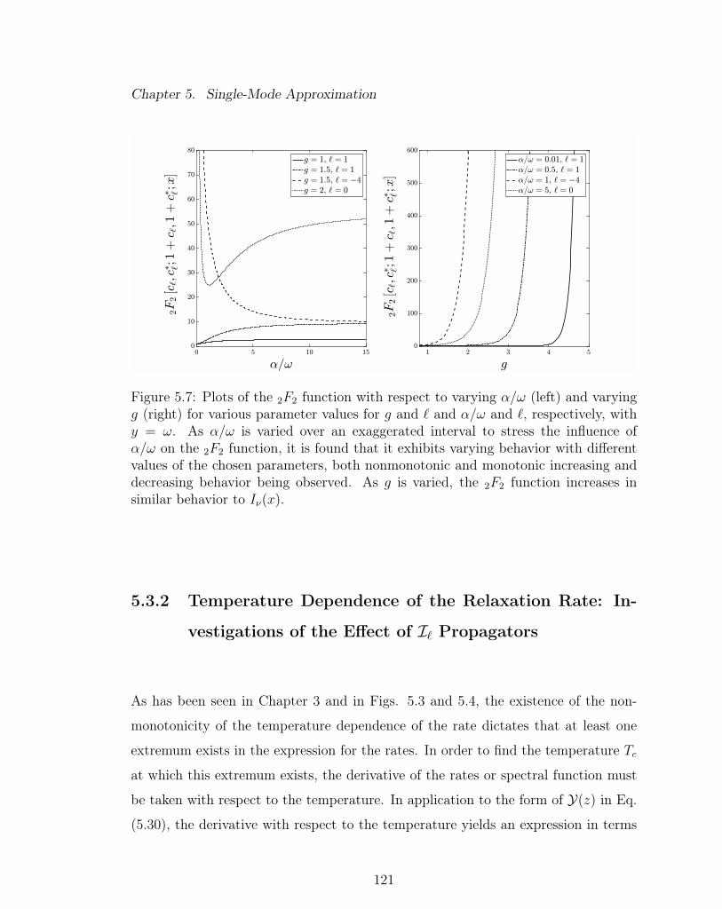
Chapter 5. Single-Mode Approximation
Figure 5.7: Plots of the 2F2 function with respect to varying α/ω (left) and varyingg (right) for various parameter values for g and ` and α/ω and `, respectively, withy = ω. As α/ω is varied over an exaggerated interval to stress the influence ofα/ω on the 2F2 function, it is found that it exhibits varying behavior with differentvalues of the chosen parameters, both nonmonotonic and monotonic increasing anddecreasing behavior being observed. As g is varied, the 2F2 function increases insimilar behavior to Iν(x).
5.3.2 Temperature Dependence of the Relaxation Rate: In-
vestigations of the Effect of I` Propagators
As has been seen in Chapter 3 and in Figs. 5.3 and 5.4, the existence of the non-
monotonicity of the temperature dependence of the rate dictates that at least one
extremum exists in the expression for the rates. In order to find the temperature Tc
at which this extremum exists, the derivative of the rates or spectral function must
be taken with respect to the temperature. In application to the form of Y(z) in Eq.
(5.30), the derivative with respect to the temperature yields an expression in terms
121

Chapter 5. Single-Mode Approximation
of the I` propagator and the corresponding A`’s as
∂Y(z)
∂ (T/T0)=g2α
2πu2e−g
2
β2csch2
(β~ω
2
)×
∞∑`=−∞
[I`−1 (x)− 2I` (x) + I`+1 (x)]A`(z − Ω). (5.33)
where T0 = ~ω/kB and x = 2g2n(ω). From the form of Eq. (5.33), it is apparent
that one of the extrema of Y(z) occurs at zero temperature due to the limiting forms
of the temperature dependent terms,
limT→0
β2csch2
(β~ω
2
)I`[2g2n(ω)
]e−2g2n(ω) → 0. (5.34)
It can also be seen that the other value(s) for which the derivative or slope of Y(z)
will be zero is dependent on the interplay of the I`(x) propagators in the sum with
the amplitude terms A`, determining the maximum value of the function at each
corresponding `.
The derivative in Eq. (5.33) may be rewritten in a different form by shifting the
indeces of the I`(x) and A` functions such that only one propagator is present in the
sum over all `’s:
∂Y(z)
∂(T/T0)=g2α
2πu2e−g
2
β2csch2
(β~ω
2
)×
∞∑`=−∞
I` (x) [A`+1(z − Ω)− 2A`(z − Ω) +A`−1(z − Ω)] . (5.35)
With the new form of the derivative it is easy to prove that all temperature dependent
components are positive for all T by the definition of the propagator as functions
of I-Bessel and decaying exponential functions of an always positive argument and
from the temperature dependent behavior of the terms outside the sum which are
also positive for all T . The sign change contribution to the derivative arises from the
sum of the A`(z)’s in the square brackets which can lead to the change in direction
of the slope depending on the value of the ` considered in conjunction with the value
of z − Ω.
122

Chapter 5. Single-Mode Approximation
For the rates, z−Ω is either ±Ω, and the value of ` is modulated in the definition
of the A`’s in Eq. (5.21) as ` ∓ Ωω. Eq. (5.35) may therefore be written to describe
the slope of the rates as
∂Γ±∂(T/T0)
=g2α
2πu2β2e−g
2
csch2
(β~ω
2
)×
∞∑`=−∞
I` (x)[A`±Ω
ω+1 − 2A`±Ω
ω+A`±Ω
ω−1
], (5.36)
the extrema for which may be found by setting the sum in Eq. (5.36) equal to zero
and solving for Tc/T0 6= 0, i.e.,
∞∑`=−∞
I` (x)[A`±Ω
ω+1 − 2A`±Ω
ω+A`±Ω
ω−1
]= 0. (5.37)
While an exact analytic form may not be possible for Tc/T0, a numerically obtained
result may be found for given values of g and Ω/ω verifying the nonmonotonic be-
havior of the rates.
123

Chapter 6
Concluding Remarks
In the main part of this dissertation, the focus has been on understanding the re-
laxation behavior of a quantum system in interaction with a thermal reservoir, the
relaxation behavior consisting of simultaneously occurring phase relaxation through
decoherence processes and population equilibration. It has been shown that the
strength of interaction, as well as the properties of the bath with which the sys-
tem is in contact, affects the relaxation of the system revealing both intuitive and
counter-intuitive behavior with changes in temperature. We have developed a theory
for understanding the short-time as well as temperature-dependent observations of
vibrational relaxation experiments of molecules embedded in thermal reservoirs.
We have given a brief introduction to the experimental methods and theoretical
tools underlying the research in this study, including a discussion of pump-probe
methods. Projection operator techniques enhanced to incorporate coarse-graining
have been employed as our theoretical tools. Both cases of weak and strong inter-
action have been considered, the strong necessitating a dressing transformation in
which the Hamiltonian is brought into a representation where the interaction is made
weak.
124

Chapter 6. Concluding Remarks
The interactions considered in this study are separable into independently con-
tributing system-operator- and bath-operator-dependent components. This results
in the expressions for the memories present in the generalized master equation to de-
pend on independent system and bath contributions. The latter simply are thermal
averages of appropriate bath quantities. Our analysis has uncovered both an intu-
itive Arrhenius temperature dependence for transition rates as well as an interesting,
and perhaps unexpected, nonmonotonic behavior.
While our focus is on optical phonon interactions, for completeness the interaction
with a bath of acoustic phonons has also been considered. Analytic results obtained
for the bath correlation functions, and hence the memories, through the use of the
Debye approximation for the acoustic phonon density of states produce expressions
in terms of special functions such as the Lerch transcendent and its variations, as
well as incomplete gamma functions, in both interaction strength regimes.
With optical phonon interactions, we have made significant progress in studying
the relaxation to equilibrium of three representative quantum systems [23,49,62,65].
We have found that the nonmonotonicity effect inherent in the relaxation rates,
Γ−, in the case of strong interaction is expressed in the temperature dependence of
the behavior of the typical observable for each system: the occupation probability
difference for the nondegenerate dimer, the steady-state value of the average velocity
of a charged particle moving across the sites of a lattice as a result of the interaction,
and the energy of the molecule represented by a harmonic oscillator.
We have derived an expression for the effective rate and relaxation memory from
the generalized form of the traditional incoherent relation for the energy of a relaxing
molecule represented by a harmonic oscillator. The effective rate derived from the
use of the microscopically derived memories in this dissertation shows interesting
behavior with increasing temperature, such as temperature dependent oscillations.
We have also applied the half-Markoffian approximation to develop a convolutionless
125

Chapter 6. Concluding Remarks
integro-differential equation which is particularly useful for analysis in extreme short-
and long-time limits.
We made a connection of the Lorentzian form of the spectral function in the strong
interaction regime to a special case of the generalized hypergeometric functions, the
2F2, which exhibits, inherently, nonmonotonic behavior that is highly dependent on
the values of the microscopically defined parameters. We showed that, in the case
of a strong interaction of a system with a bath of optical phonons approximated by
a single mode of vibration with the introduction of disorder, at least one extremum
other than at zero temperature exists in the expression for the spectral function,
and hence the transition rates. The existence of a critical temperature at which the
slope of the rates changes direction further demonstrates the existence of an inherent
nonmonotonicity in the expressions for the rates.
Planned future work following this dissertation includes the application of the
theory presented here to the experiments reported on by Fayer et. al. and, addi-
tionally in a different context, a first-principles analysis of experiments such as those
addressed in Appendix B by the methods of granular hydrodynamics.
126

Appendices
A Microscopic Connection to Phenomenological Memories 128
A.1 Single Mode of Vibration . . . . . . . . . . . . . . . . . . . . . . . . 129
A.2 Lorentzian Spectral Function . . . . . . . . . . . . . . . . . . . . . . 131
A.3 Gaussian Spectral Function . . . . . . . . . . . . . . . . . . . . . . . 132
B Investigation of the Classical Problem of Granular Materials 135
B.1 Introduction . . . . . . . . . . . . . . . . . . . . . . . . . . . . . . . 136
B.2 Surface Profile Calculations In The Rotating Drum . . . . . . . . . . 138
B.3 Comparison to Experiment . . . . . . . . . . . . . . . . . . . . . . . 149
127

Appendix A
Microscopic Connection to
Phenomenological Memories
In their study, Kenkre and Chase [23] introduce phenomenological baths, not derived
from microscopic details, in order to study the effect of the system-bath interaction
on the relaxation behavior of the system. The phenomenological baths considered
are introduced through postulated spectral functions Y(z) chosen to ensure that they
satisfy the detailed balance condition of
Y(z) = eβ~zY(−z). (A.1)
A catalog of the various spectral functions and resultant phenomenologically derived
memories is given in ref. [23], where the corresponding memories are found through
the relationship,
κφ±(t) =
∫ ∞−∞
dz Y(z) cos [(z ± Ω) t] . (A.2)
In Chapter 3 of the present dissertation, microscopically defined baths were con-
sidered for which the corresponding bath spectral functions have been derived. We
use them in this Appendix to derive relations to three phenomenologically deduced
128
Appendix A. Microscopic Connection to Phenomenological Memories
bath spectral functions in ref. [23], the three being a single mode of vibration, a
Lorentzian, and a Gaussian spectral function.
A.1 Single Mode of Vibration
In ref. [23], the first bath considered is one which is described by a triple delta
function
Y(z) =2
1 + e−β~z
[Hδ(z) + (1−H)
δ (z − Ω) + δ (z + Ω)
2
], (A.3)
(Eq. (32) in ref. [23]). Unlike in ref. [23] where H is set to 1/2, here H is set to 0.
The spectral function in this case may be rewritten as
Y(z) =1
1 + e−β~z[δ (z − Ω) + δ (z + Ω)] , (A.4)
and when the normalizing constant in Eq. (A.4) is carried out, with the application
of the arguments in the delta functions, the spectral function takes the form
Y(z) = nf (Ω)[eβ~Ωδ (z − Ω) + δ (z + Ω)
]. (A.5)
Here, nf (Ω) =(1 + eβ~Ω
)−1 is the Fermi occupation number. The corresponding
memories derived from the phenomenological bath postulated in Eq. (A.4) (setting
H = 0 in the equation following Eq. (32) in ref. [23]) have the form,
φ±(t) = cos2 (Ωt)∓ tanh
(β~Ω
2
)sin2 (Ωt) ,
or
φ±(t) = nf (Ω) eβ~Ω
2
[e±
β~Ω2 + e∓
β~Ω2 cos (2Ωt)
]. (A.6)
In Chapter 3, the microscopic memories were introduced for the case of the weak
interaction of a nondegenerate system of characteristic frequency Ω with a bath of
129

Appendix A. Microscopic Connection to Phenomenological Memories
phonons. In the case of the interaction with a single mode of vibration of frequency
ω, the bath correlation function is found in terms of the phonon occupation number,
n(ω), as
B(t) = g2~2ω2n(ω)[eβ~ωeiωt + e−iωt
], (A.7)
with the corresponding memories being
κφ±(t) = g2ω2n(ω)[eβ~ω cos ([Ω± ω] t) + cos ([Ω∓ ω] t)
]. (A.8)
In the case in which ω = Ω is considered, the microscopically derived memories in
Eq. (A.8) may be rewritten as
κφ±(t) = g2Ω2n(Ω)eβ~Ω
2
[e±
β~Ω2 + e∓
β~Ω2 cos (2Ωt)
](A.9)
which are easily comparable to the phenomenologically deduced memories in Eq.
(A.6), the two equations being equal excluding some normalization factors. The
corresponding bath spectral function which may be computed through the applica-
tion of Eq. (3.10), is found to be the sum of two shifted delta functions of different
amplitudes, the ratio of which satisfy the detailed balance condition,
Y(z) = g2ω2n(ω)eβ~ω
2
[eβ~ω
2 δ (z − [Ω + ω]) + e−β~ω
2 δ (z − [Ω− ω])]. (A.10)
When evaluated at the proper frequency values with ω = Ω, Eq. (A.10) yields for
the transition rates
Γ± = πg2ω2n(ω)eβ~ω
2
[e±
β~ω2 δ (Ω) + e∓
β~ω2 δ (0)
]. (A.11)
It is clear from the above calculations that the phenomenologically conjectured bath
obtained in Eq. (32) of ref. [23] can be substantiated by microscopic prescriptions, as
the spectral functions obtained from microscopically derived memories for the case
of the weak interaction with a single mode of vibration where ω = Ω is equivalent to
the phenomenologically obtained one, barring some normalization factors.
130

Appendix A. Microscopic Connection to Phenomenological Memories
A.2 Lorentzian Spectral Function
Another phenomenological bath deduced in ref. [23] which may be substantiated
by microscopically derived memories is that of the Lorentzian centerted about the
origin (Eq. (37) of ref. [23])
Y(z) =1
π
(1 + e−β~Ω
1 + e−β~z
)(Ω2 + α2
α2 + z2
), (A.12)
where the width w has been replaced by α. The corresponding expressions for the
memories have been derived in ref. [23] to have the forms
φ±(t) =
(1 + e−β~Ω
2
)(Ω2 + α2
α
)[(cos Ωt∓ tan
β~α2
sin Ωt
)e−αt (A.13)
∓ 4 sin Ωt∞∑n=0
[β~α
β2~2α2 − π2(2n+ 1)2
]e−π(2n+1)t
β~
]
The symmetric form of Eq. (A.12) given by
Ys(z) =(1 + e−β~z
)Y(z) = Y(z) + Y(−z) (A.14)
is given by the relation
Ys(z) =1
π
(1 + e−β~Ω
)(Ω2 + α2
α2 + z2
). (A.15)
The cosine Fourier transform over z of the symmetric form of the spectral function,
in general, yields the sum of the memories [23], i.e.,
WS(t) =W−(t) +W+(t) =
∫ ∞−∞
dz Ys(z) cos [(Ω + z) t] . (A.16)
WS(t) = κΩ2 + α2
αe−
β~Ω2 cosh
(β~Ω
2
)e−αt cos (Ωt) . (A.17)
If instead we consider the same form of the symmetric spectral function as in Eq.
(A.15), but with the center being about a nonzero bath frequency of ω, i.e.,
Ys(z) =1
π
(1 + e−β~Ω
)( Ω2 + α2
α2 + (z − ω)2
), (A.18)
131

Appendix A. Microscopic Connection to Phenomenological Memories
the corresponding expression for the sum of the memories paralleled in Eq. (A.17)
is found as
WS(t) = κΩ2 + α2
αe−
β~Ω2 cosh
(β~Ω
2
)e−αt cos [(Ω + ω) t] . (A.19)
The forms obtained in Eq. (A.19) are reminiscent of the memories obtained for the
case of weak interaction with a single mode of vibration with the introduction of
disorder not taken explicitly into account in the microscopically defined Hamiltonian
or the forms describing the weak interaction with an optical phonon band with a
Lorentzian frequency density of states with very narrow dispersion, both of which
yield the same expression for the sum of the memories
WS(t) = 2g2ω2 coth
(β~ω
2
)e−αt cos [(Ω + ω) t] + cos [(Ω− ω) t] . (A.20)
The microscopically derived memories are dependent on the sum and difference of the
system characteristic and phonon frequencies, displaying detailed balance which not
only arises in the frequency spectrum of the two components of the associated spectral
function involved but also in the ratio of the transition rates (at least for higher
temperatures as seen in Chapter 5). The phenomenologically obtained versions of
the memories depend only on the sum of the frequencies, displaying detailed balance
in the ratio of the associated transition rates. While there are differences between
the two forms, including multiplicative factors, it is clear that the behavior of the
phenomenologically obtained memories in Eqs. (A.19) have some microscopic basis
when compared to the microscopically derived forms in Eqs. (A.20).
A.3 Gaussian Spectral Function
Yet another phenomenological bath deduced in ref. [23] which may be substantiated
by microscopically derived memories is that of the Gaussian spectral function defined
132

Appendix A. Microscopic Connection to Phenomenological Memories
in Eq. (48) of ref. [23] as
Y(z) =1
π
(1 + e−β~Ω
1 + e−β~z
)e−
z2−Ω2
2σ2 , (A.21)
where the width w has been replaced by√
2σ. The corresponding expressions for
the memories have been derived in ref. [23] to have the forms
φ±(t) =1 + e−β~Ω
4
√2
πσe
Ω2
2σ2
[e−
σ2t2
2 cos Ωt± i(w(σt√
2
)− w
(− σt√
2
))sin Ωt
+ 2i sin Ωt∑n=1
(−1)n(w(σt+ inβ~σ√
2
)− w
(−σt+ inβ~σ√
2
))],
(A.22)
where w(iz) = exp(z2)erfc(z) is the Faddeeva function [59].
If we look at the symmetric form of the spectral function which has the form
Ys(z) =1
π
(1 + e−β~Ω
)e−
z2−Ω2
2σ2 , (A.23)
the expression for the sum of the memories may be found as
WS(t) = κe−β~Ω
2 cosh
(β~Ω
2
)√2
πσe
Ω2
2σ2 e−σ2t2
2 cos (Ωt) . (A.24)
For the case in which the spectral function is centered about a nonzero frequency,
i.e.,
Ys(z) =1
π
(1 + e−β~Ω
)e−
(z−ω0)2−Ω2
2σ2 , (A.25)
the expression for the sum of the memories may be found as
WS(t) ∝ cosh
(β~Ω
2
)e−
σ2t2
2
×[(
1 +σ2
ω20
− σ4t2
ω20
)cos (ω0t)− 2
σ2
ω0
t sin (ω0t)
]cos (Ωt) . (A.26)
The forms obtained in Eq. (A.24) are reminiscent of the memories obtained for
the case of weak interaction with an optical phonon band described by a Gaussian
133
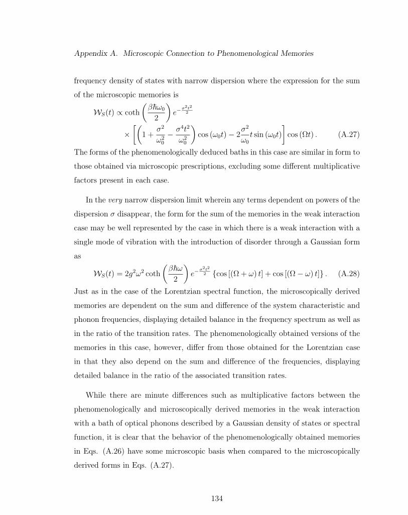
Appendix A. Microscopic Connection to Phenomenological Memories
frequency density of states with narrow dispersion where the expression for the sum
of the microscopic memories is
WS(t) ∝ coth
(β~ω0
2
)e−
σ2t2
2
×[(
1 +σ2
ω20
− σ4t2
ω20
)cos (ω0t)− 2
σ2
ω0
t sin (ω0t)
]cos (Ωt) . (A.27)
The forms of the phenomenologically deduced baths in this case are similar in form to
those obtained via microscopic prescriptions, excluding some different multiplicative
factors present in each case.
In the very narrow dispersion limit wherein any terms dependent on powers of the
dispersion σ disappear, the form for the sum of the memories in the weak interaction
case may be well represented by the case in which there is a weak interaction with a
single mode of vibration with the introduction of disorder through a Gaussian form
as
WS(t) = 2g2ω2 coth
(β~ω
2
)e−
σ2t2
2 cos [(Ω + ω) t] + cos [(Ω− ω) t] . (A.28)
Just as in the case of the Lorentzian spectral function, the microscopically derived
memories are dependent on the sum and difference of the system characteristic and
phonon frequencies, displaying detailed balance in the frequency spectrum as well as
in the ratio of the transition rates. The phenomenologically obtained versions of the
memories in this case, however, differ from those obtained for the Lorentzian case
in that they also depend on the sum and difference of the frequencies, displaying
detailed balance in the ratio of the associated transition rates.
While there are minute differences such as multiplicative factors between the
phenomenologically and microscopically derived memories in the weak interaction
with a bath of optical phonons described by a Gaussian density of states or spectral
function, it is clear that the behavior of the phenomenologically obtained memories
in Eqs. (A.26) have some microscopic basis when compared to the microscopically
derived forms in Eqs. (A.27).
134

Appendix B
Investigation of the Classical
Problem of Granular Materials
This Appendix describes research results obtained on a topic totally unrelated to
the main subject of this dissertation. The topic is the classical problem of the flow
of granular material inside a rotating drum. The research was completed before the
studies of vibrational relaxation were undertaken.
A brief introduction to the topic of granular material is given in the first Section,
discussing the importance of rheology which is the study of the flow of granular
matter. A summary is then given of some of the specific systems used in the study.
Following that, the theory involved in modeling the S-shaped profile of granular
material inside a rotating drum which has been developed by Endicott et. al. in
refs. [79, 80] is introduced along with recent analytical extensions and results in
which a radius-dependent flow layer thickness has been incorporated.
135

Appendix B. Investigation of the Classical Problem of Granular Materials
B.1 Introduction
Granular materials have attracted much attention in the past century in both the
scientific and engineering communities due to their applicability and complexity.
Engineers have interest in granular materials because of their use in industrial pro-
cesses, whereas physicists (who have only in the past few decades taken an interest
in the “matter”) are interested in the statistical mechanics and critical phenomena
that take place during such processes. The late Nobel laureate, Pierre de Gennes
stated that “[g]ranular matter, in 1998, [was] at the level of solid-state physics in
1930” [81]. Granular materials, that is, materials composed of macroscopic particles
such as sand, powders, gravel, and pills, have the unique property of experiencing not
only behavior definitive of a solid, but liquid and gas-like behavior as well [82, 83].
Within each of these material phases, granular material exhibits properties which are
unique to each of the three states. For instance, when the grains within a granular
material have strong interaction with one another and are almost stationary, the
granular material as a whole is treated as a solid. If, on the other hand, the grains
move freely with little or no interaction with each another, it may be treated as a
liquid or gas.
Ralph Alger Bagnold launched the journey into the search of an understanding
of the mechanics and dynamics of granular material in 1941 with his book “The
Physics of Blown Sand and Desert Dunes” which focuses on the physics of the pat-
tern formation and wind transportation of sand on the dunes in the Libyan desert
[84]. Since then much research and experimentation has proceeded in an effort to
understand the complexity of the mechanics and equilibrium properties of granular
material systems such as vibrated powders [85–90], stress distribution during com-
paction [91–99], surface profiles of flows of granular material within various systems
[80,100–102], segregation and/or mixing of two or more dissimilar types of granular
materials due to agitation [103–112], and studies of the theory and application of
136

Appendix B. Investigation of the Classical Problem of Granular Materials
NMR microscopy used as an experimental probe [113–121] in granular matter. Such
studies are of importance in industries that involve the processing, transportation,
and mixing of granular materials such as, for example, the mixing of powders and
transportation of pills in the pharmaceutical industry, the transportation of bulk
commodities, such as cereals, grains, coffee, and sugar in the food industry, and the
mixing of cement and concrete as well as the moving of sand and gravel in the con-
struction industry. Studies performed on the stress distribution and flow of granular
material are of interest also in avalanche, earthquake, and landslide prevention stud-
ies [83] where interest lies in initiating small avalanches or earthquakes in order to
prevent major disasters.
In the industry, many systems are used for processing, transporting, and/or stor-
ing these materials, including funnels, silos, rotary kilns, and vibration beds [83,102].
Of interest in this Appendix is the flow of granular material, in particular the shape
of the flow layer inside of a continuously rotating drum. The simpler counterpart to
this system is the illustrative sand heap or sand on an inclined plane. Texts such
as ref. [83] begin the discussion of the flow of material with examples such as that
of sand flowing along an inclined plane. If the angle of inclination α of the inclined
plane is below a certain threshold angle θc (called the “angle of repose”) the sand will
remain stationary on the surface and act as a solid. If, however, α is increased above
θc, the sand will begin to slide or flow along the surface, acting as a liquid.
Consider now instead the case of the sand heap wherein sand is added to the top,
either by pouring or some other external agitation. Here the same effect is observed.
As sand is added, the angle of inclination between the horizontal and the surface of
the sand heap increases, and once the critical angle is reached, the sand begins to flow
along the surface, and the flow continues until the heap angle of inclination decreases
to below θc. In both cases the flow layer acts as a dynamic non-Newtonian fluid,
i.e., a fluid which displays variable viscosity with applied force, exhibiting variable
137

Appendix B. Investigation of the Classical Problem of Granular Materials
phase state behavior within and along the various flow layers. The sand heap as
a whole system, for instance, has both a dynamic and static property in that the
motion only occurs at the surface, an “active layer” (liquid phase), while the rest
remains stationary, a “passive layer” (solid state). From this, it is concluded that
θc is highly dependent on the transition between the solid and liquid state of the
granular material in question [83,101].
Using this idea of the sand heap, we consider in this Appendix the practical system
of a partially filled cylindrical drum with non-slip walls found in many industries
that require mixing of materials, e.g., the construction, food, and pharmaceutical
industries. As the cylinder is rotated about its cylindrical axis similar behavior
to the sand heap and sand on an inclined plane is displayed wherein the formerly
horizontal surface begins to rise in inclination until reaching some critical angle at
which granular flow begins. As the level of one end of the surface rises due to the
rotation, it will eventually reach that threshold and undergo an avalanche, until the
speed of rotation is increased, bringing the angle of inclination to and above θc to
form a continuous flow.
B.2 Surface Profile Calculations In The Rotating
Drum
In 1990, Rajchenbach described the flow of powders within a half-filled rotating
drum of radius R as experiencing hysteresis in the transition between the discrete
avalanche and continuous regimes [100]. At low rotation speeds Ω, the slope of the
profile increases until an avalanche occurs yielding a discrete regime, and at high
rotation speeds the flow becomes continuous and a steady profile is observed. These
regimes are given characteristic rotation speeds which attribute to the fall time of
138

Appendix B. Investigation of the Classical Problem of Granular Materials
one particle in the transition between the two regimes. When the rotation speed is
then increased above the characteristic speed for a continuous flow regime, that is,
when Ω ≥ Ω+ rpm, the rectilinear profile becomes S-shaped.
The S-shaped profile of the free surface flow on the top of the granular bed of a
rotating cylinder has been examined by many in the literature such as Rao et. al.
[104], Zik et. al. [105], Kenkre et. al. [80], Orpe and Khakhar [101], Taberlet et. al.
[122], and Sanfratello et. al. [123]. Much of the literature focuses on experimental
results and fitting models/equations to the data, whereas some research focuses on
the modeling and understanding of the mechanics and dynamics involved within the
flow layer of a half-filled rotating cylinder. For simplicity in modelling, and without
loss of generality, the problem of the partially filled rotating cylinder is typically
reduced to that of a two-dimensional problem by taking a cross-sectional area of the
system. Within that cross-section the flow layer, sometimes called the “active” layer,
is taken to exhibit fluid-like motion while the rest of the material is considered to
exhibit total rigid body motion acting as a “passive” layer. This is done in agreement
with many experimental results and evidence given by Sanfratello et. al. in [121,123]
in which MRI velocimetry measurements of the velocity depth profile were made,
showing the quadratic behavior of the velocity within the active layer and the rigid
body motion of the passive layer.
B.2.1 Theory for Profile Prediction
Kenkre et. al. [80] used the fact that the system exhibits total rigid body motion after
some depth from the flow surface in their analysis of the problem of the partially filled
rotating cylinder. Their formalism begins with an assumption made in the literature
by several authors [106–108,110,122,123], wherein the motion is considered to be that
of total rigid body motion of the material within the passive layer with a continuous
source of particles to the top and a constant sink of particles in the bottom half of the
139

Appendix B. Investigation of the Classical Problem of Granular Materials
Figure B.1: Cross-sectional view of partially-filled rotating cylinder of radius R,rotation speed Ω, and layer thickness ∆.
flow layer. The flow layer is considered to be of a single species of granular material
in which the continuum expressions for the conservation of mass and momentum are
defined along the direction of flow of the material within the layer, incorporating the
properties of the material itself.
The particle density of the single species of granular material, ρ, is taken to be
constant throughout both layers. As the cylinder is rotated about its axis, the passive
portion of the material exhibits rigid body motion with velocity Ωr where Ω and r
are the rotation speed of the cylinder about and the radial distance from the axis
(see Figure B.1). The normal component of the rigid body velocity to the flow layer,
v⊥ = Ωrdr
ds, (B.1)
is taken to be constant at the transition surface which lies between the rigid body
and flow layers and is taken to decrease throughout the flow layer. Here ds is the
infinitesimal arc length along the profile and dr is the infinitesimal radial distance
140

Appendix B. Investigation of the Classical Problem of Granular Materials
Figure B.2: Zoomed-in section of profile.
defining the arc length.
On crossing the transition surface from the rigid body to the flow layer and vice
versa, the particles are assumed to take on the momentum of the particles occupying
the region in which they have entered. The flux within the flow layer has the same
form throughout
j = ρvs, (B.2)
where vs is the average particle velocity within the layer. The influx of particles,
i.e., the particles that provide the constant source into the layer coming through
the transition surface into the fluid layer at the top, and the outflow of particles
at the bottom, i.e., the particles that sink back into the rigid body region toward
the bottom half of the flow, are taken to have the same flux form, increasing in the
direction of increasing polar angle,
ji(r) = ρΩrϑ. (B.3)
While material from the passive layer emerges in the direction of ϑ which is
normal to r, its component along the normal to the profile, i.e., the n direction,
serves as the input to the active layer. Taking the dot product of the influx vector
with the normal to the surface of the profile, the relation for the normal component
141

Appendix B. Investigation of the Classical Problem of Granular Materials
of the incoming flux is found to be
ji,⊥ = ji · n = −ρΩrdr
ds. (B.4)
It is easily seen that the volume integral of flux within the flow layer (i.e., the integral
over the depth and length of the layer in the appropriate directions) is equivalent
to the surface integral of the normal component of ji. Solving these integrals for
the flux of the particles within the layer leads to the de Gennes relation for the flux
within the layer of
j(r) =1
2ρ
Ω
∆
(R2 − r2
), (B.5)
and an explicit expression for the velocity of the particles within the flow layer can
be extracted as
vs =1
2
ΩR2
∆
(1− r2
R2
). (B.6)
It is stressed in the discussion of Kenkre et. al. [80] that this particular relation
for the flux holds true for all profile geometries as the profile shape is defined within
the parameter of
dr
ds=
x+ y dydx
r
√1 +
(dydx
)2, (B.7)
where
r =√x2 + y2 (B.8)
and
dy
dx= tan θ. (B.9)
Here θ is the angle made by the free surface with the horizontal. It is also stressed
that the fraction of the cylinder that is filled with granular material, defined as the
filling fraction
f =Across-section − Afilled
Across-section= 1− 1
π
(cos−1
( cR
)− c
R
√1−
( cR
)2), (B.10)
142

Appendix B. Investigation of the Classical Problem of Granular Materials
where c is the distance between the axis of rotation and the top of the surface of the
material when the cylinder is stationary, does not affect the profile itself.
The result for the flux within the active layer reflects the idea of mass-balance
equations or, more generally, the conservation equation of
∂(Qρ)
∂t+
d
ds(Qρvs) + S = F (B.11)
in which S is the source or sink term arising from the rigid body rotation defined as
S = vsρΩ
∆rdr
ds, (B.12)
Here, F denotes the rate of creation of Qρ. With Q = 1 and F = 0, the general
steady-state equation of mass balance is recovered, whereas with Q = vs , the ve-
locity of the flowing particles along the free surface, F becomes the total force per
unit volume acting on the granular particles along the profile curve. This force is
composed of the component of gravity along the free surface, viz., g sin θ, the dry
friction which acts against the motion and equals the product of the coefficient of
kinetic friction µ and the normal reaction g cos θ, and a damping force which opposes
motion and arises from collisions of the granular particles with others, a simple model
of which gives the phenomenological force of −γρvs.
The final form of the equation used to model the flow within the layer is then
∂(ρvs)
∂t+
d
ds
(ρv2
s
)+ vsρ
Ω
∆rdr
ds= ρ [g (sin θ − µ cos θ)− γvs] (B.13)
which in steady state becomes
d(ρv2s)
ds+ vs
Ω
∆rρdr
ds= ρ [g (sin θ − µ cos θ)− γvs] . (B.14)
and has the solution for the slope dy/dx of
dy
dx= −a(x, y)b(x, y)
a2(x, y)− γ2±γ√a2(x, y) + b2(x, y)− γ2
a2(x, y)− γ2, (B.15)
143

Appendix B. Investigation of the Classical Problem of Granular Materials
where
a(x, y) =Ω
∆y +
g
vs, and b(x, y) =
Ω
∆x− µ g
vs. (B.16)
Eq. (B.16) is solved numerically and profiles of y versus x are plotted. In general,
the expression for dy/dx defines the slope all along the profile surface and would make
sense that at the boundary, where j(r = R) = 0 and hence vs(r = R) = 0, the slope
would be equal to the coefficient of kinetic friction as this is the requirement for the
particles to begin to flow down the incline, that is,
dy
dx
∣∣∣r=R
= tan θc = µ. (B.17)
This is the case for this formalism and it is found that as r → R, dy/dx→ µ.
B.2.2 Present Analysis and Results
The assumption made in Kenkre et. al. [80], that the flow layer has a constant
thickness ∆, arose from a perceived need for a simplification. The present analysis,
given below, shows that this simplification is unnecessary. It is relaxed to show that
results compatible with observations can be obtained by generalizing the arguments
to include an r-dependent ∆ taken from experimental observations [107, 118, 123].
Imaging done by Khakhar et. al. in [107] shows that the depth of the profile is
not constant throughout the layer, but should increase as a quadratic, that is, the
equation of the layer thickness should have a form similar to
∆(r) = ∆0
√1− r2
R2, (B.18)
where ∆0 is some maximum thickness measured from the top of the active layer
surface, R is the radius of the cylinder, and r is the radial distance from the cylinder’s
axis of rotation to the flow layer.
144

Appendix B. Investigation of the Classical Problem of Granular Materials
The flux within the layer, therefore, with the implementation of the newly defined
layer thickness is found to be
j(r) = ρvs =1
2ρ
ΩR2
∆(r)
(1− r2
R2
), (B.19)
where the expression for the velocity for the particles within the flow layer can be
extracted as
vs(r) =1
2
ΩR2
∆(r)
(1− r2
R2
), (B.20)
where ∆(r) is as in Eq. (B.18). At the center of the flow layer, i.e., r = 0, the
velocity takes on its maximum value of
vs,max =1
2
ΩR2
∆0
, (B.21)
This is in agreement with evidence given by Sanfratello et. al. in ref. [123], showing
the quadratic behavior of the velocity within the active layer, and experimental
results of Caprihan and Seymour [118] wherein the layer thickness, velocity vs, and
hence the flux within the layer are all 0 at the boundary, a condition with which the
de Gennes result was obtained in the first place.
Invoking the conservation of momentum in terms of macroscopic bulk flow vari-
ables as before, the above functions are implemented into the steady-state momentum
balance equation yielding
d(ρv2s)
ds+ vs
Ω
∆(r)rρdr
ds= ρ [g (sin θ − µ cos θ)− γvs] (B.22)
and a similar expression for the slope dy/dx of ref. [80] is obtained
dy
dx= − a(x, y)b(x, y)
a2(x, y)− c2(x, y)±c(x, y)
√a2(x, y) + b2(x, y)− c2(x, y)
a2(x, y)− c2(x, y), (B.23)
where, with $ = vs,max/R = ΩR/(2∆0),
a(x, y) = $2y + g, b(x, y) = $2x− µg, (B.24)
145
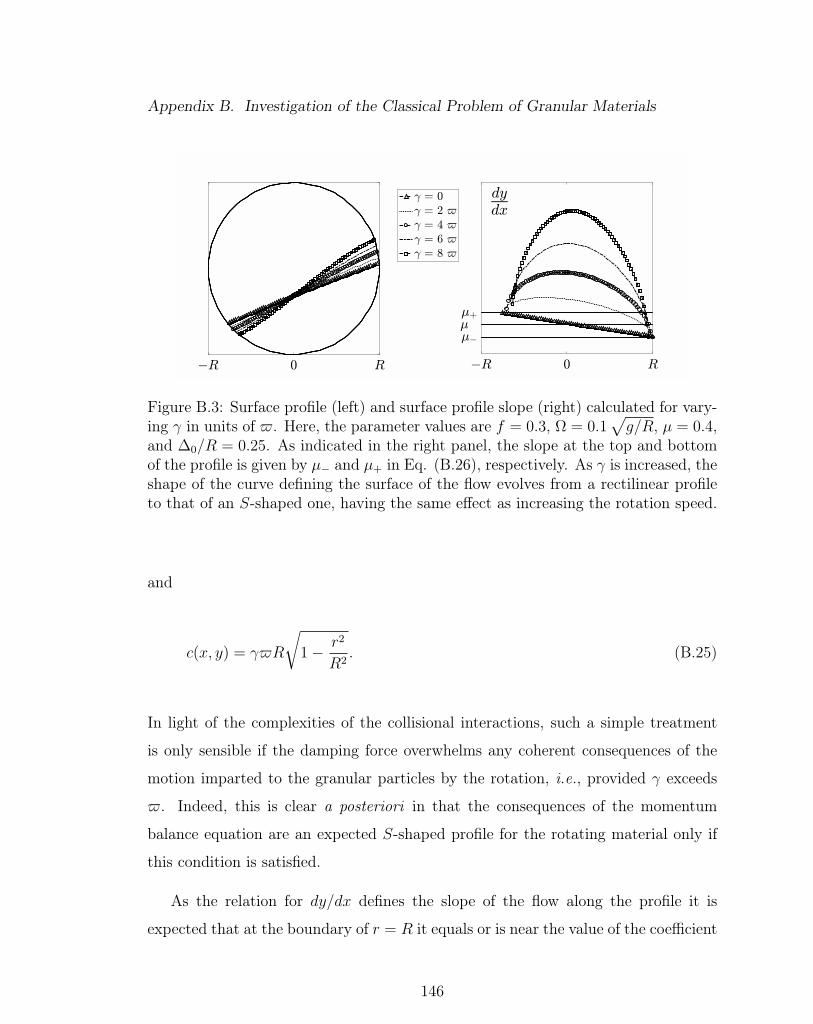
Appendix B. Investigation of the Classical Problem of Granular Materials
Figure B.3: Surface profile (left) and surface profile slope (right) calculated for vary-ing γ in units of $. Here, the parameter values are f = 0.3, Ω = 0.1
√g/R, µ = 0.4,
and ∆0/R = 0.25. As indicated in the right panel, the slope at the top and bottomof the profile is given by µ− and µ+ in Eq. (B.26), respectively. As γ is increased, theshape of the curve defining the surface of the flow evolves from a rectilinear profileto that of an S-shaped one, having the same effect as increasing the rotation speed.
and
c(x, y) = γ$R
√1− r2
R2. (B.25)
In light of the complexities of the collisional interactions, such a simple treatment
is only sensible if the damping force overwhelms any coherent consequences of the
motion imparted to the granular particles by the rotation, i.e., provided γ exceeds
$. Indeed, this is clear a posteriori in that the consequences of the momentum
balance equation are an expected S-shaped profile for the rotating material only if
this condition is satisfied.
As the relation for dy/dx defines the slope of the flow along the profile it is
expected that at the boundary of r = R it equals or is near the value of the coefficient
146

Appendix B. Investigation of the Classical Problem of Granular Materials
Figure B.4: Surface profile calculated for low (left) and high (right) rotation speeds.Here the parameter values are Ωlow/Ωhigh = 0.1, γ/Ω = 10, µ = 0.2, and ∆0/R =0.15.
of kinetic friction. It is found that its boundary value is of the form
µ± =dy
dx
∣∣∣r=±R
=µ
1−($2
gR)2
1∓ $2R
µg
√1 + µ2 −
($2
gR
)2 (B.26)
where µ± represents the slope at the bottom and top boundaries of the flow, re-
spectively. Under the right conditions, i.e., $2 µg/R, Eq. (B.26) may be ap-
proximated by µ. Indeed what is observed with the variation of rotation speed and
damping parameter is that the slope of the profile varies tremendously with respect
to µ along the horizontal, with a peak slope occurring away from x = 0 and closer
tothe top of the flow. In Fig. B.3, a filling fraction of 0.3 is chosen to show the effect
of the variation of the damping factor, γ, on the shape of the surface profile and
change in the slope along the surface. As γ is increased, the effect on the shape of
the profile is similar to that expected with an increase in the rotation speed [100],
wherein the surface profile evolves from rectilinear to an S shape.
Solving Eq. (B.23) numerically, the profile for low rotation speed Ω for a half-
147

Appendix B. Investigation of the Classical Problem of Granular Materials
Figure B.5: Surface profile and surface profile slope calculated for varying Ω in unitsof γ. Here the parameter values are f = 0.3, γ = 4
√g/R, µ = 0.4, and ∆0/R = 0.25.
As shown in the right panel, the slope along the surface of the flow layer changesdrastically with increasing rotation speed, with the peak of the slope occurring awayfrom x = 0 and close to the top of the flow layer. As the rotation speed is increased,the shape of the surface changes from rectilinear to S-shaped.
filled cylinder is plotted showing a rectilinear flow layer with quadratic depth similar
to those seen in the experiments by Khakhar et. al. [107] (see Figure B.4). As
the rotation speed is increased, the profile takes the S-shaped form as discussed in
much of the literature and experimental results [80, 100, 104, 105, 122, 123]. At the
boundaries, the layer thickness is observed to disappear or becomes infinitesimally
small which is also in agreement with much of the literature and experimental results.
The effect of the change in the rotation speed on the shape of the surface profile and
change in the slope with respect to the horizontal is shown in Fig. B.5. As the
rotation speed increases, the shape of the profile changes from a rectilinear shape to
that of an S-shape.
148

Appendix B. Investigation of the Classical Problem of Granular Materials
Figure B.6: Experimental data taken from ref. [102] and replotted in comparisonwith the profile predicted from the theoretical framework in Section B.2. In theleft panel, the surface profile is shown for the case in which the material is made ofsteel beads with a coeffiecient of kinetic friction of µ = 0.42, cylinder radius R = 20cm, layer thickness ∆0 = 4 cm, rotation speed Ω ≈ 3.13 rot/s, and the dampingcoefficient is chosen for the best fit as γ = 50$. In the left panel, the surface profileis shown for the case in which the material is made of steel and aluminum beadswith a coeffiecient of kinetic friction of µ = 0.40, cylinder radius R = 22.5 cm, layerthickness ∆0 ≈ 6.5 cm, rotation speed Ω ≈ 0.625 rot/s, and the damping coefficientis chosen for the best fit as γ = 11.75$.
B.3 Comparison to Experiment
The theory presented in this Appendix pertains to cross-sections at the center of
long cylinders wherein end wall effects are not taken into account. Many of the
experiments performed, however, were done using short cylinders where the side wall
effects were large and the theoretical accompaniment to those experiments took end
wall effects into account. The wall effects merely make the profile more pronounced
and sharper at the boundaries, that is, at r = ±R, as seen in the comparison of the
data attained by GDR MiDi [102] for steel beads and the plot of the profile using
the present formalism with the same parameters for bead diameter, rotation speed,
and cylinder radius as in ref. [102] (see Fig. B.6).
149

Appendix B. Investigation of the Classical Problem of Granular Materials
Figure B.7: Surface profile of flow layer with parameters found in recent experimentperformed by Caprihan and Seymour [118] — f = 0.5, Ω = 2.3 rad/s, R = 35 mm,∆0 ≈ 12.5 mm — according to our formalism (left) with µ = 0.4 and γ = 10$and seen by “thermal” imaging (right). The image on the right measures the axialcorrelation time calculated from image data applying the Ornstein-Uhlenbeck processdescribing Brownian particle velocity. It is a good representation of the shape of the“active” layer due to the motion of the particles (see [118]) .
The current calculation, however, only focuses on the profile shape within the
cylinder away from the end walls. Caprihan and Seymour [118] took velocity mea-
surements of a 20 mm section at the center of a long rotating half-filled cylinder with
a radius of 35 mm. The maximum depth of the profile was found to be about 12
mm and the rotation speed was taken to be 2.3 rad/s. The surface profile with such
parameters has the form (according to our formalism) which correlates to “thermal"
(pulsed-field-gradient NMR) imaging done in [118] and the predicted surface profile
using the present prescription with sed parameters is plotted in Fig. B.7, where, for
the best fit, the coefficient of kinetic friction is taken to be µ = 0.4 with a damping
parameter of γ = 10$.
It is to be stressed that the present calculations, as well as those in the earlier
work of Kenkre et. al. [80], are analytical and predict the surface profile as a slope
150

Appendix B. Investigation of the Classical Problem of Granular Materials
expression in terms of known quantities such as the cylinder radius, filling fraction,
velocity of rotation, and layer thickness. The numerical work involved is only in a
simple solution of the first order differential equation and consequent plotting. The
usefulness of the calculation is, it is hoped, in understanding further complexities
such as segregation.
151

References
[1] Wolfgang Demtröder, Laser Spectroscopy: Basic Concepts and Instrumentation,
Springer-Verlag Berlin Heidelberg, 1996.
[2] Jeanne L. McHale, Molecular Spectroscopy, Prentice Hall, University of Idaho, 1999.
[3] David W. Oxtoby, Vibrational Relaxation in Liquids, Annual Review of Physical
Chemistry 32 (1981October), 77–101.
[4] J. C. Owrutsky, D. Raftery, and R. M. Hochstrasser, Vibrational Relaxation Dynamics
in Solutions, Annual Review of Physical Chemistry 45 (1994October), 519–555.
[5] A. Tokmakoff, B. Sauter, and M. D. Fayer, Temperature-Dependent Vibrational Re-
laxation in Polyatomic Liquids: Picosecond Infrared Pump-Probe Experiments, The
Journal of Chemical Physics 100 (1994June), no. 12, 9035–9043.
[6] Elliot W. Montroll and Kurt E. Shuler, Studies in Nonequilibrium Rate Processes.
I. The Relaxation of a System of Harmonic Oscillators, The Journal of Chemical
Physics 26 (1957March), no. 3, 454–464.
[7] V. M. Kenkre and R. S. Knox, Generalized-Master-Equation Theory of Excitation
Transfer, Physical Review B 9 (1974June), no. 12, 5279–5290.
[8] V. M. Kenkre, The Generalized Master Equation and its Applications, in Statistical
Mechanics and Statistical Methods in Theory and Application, Uzi Landman (ed.),
Plenum Press, New York, NY, 1977, p. 441–461.
152

REFERENCES
[9] E. J. Heilweil, M. P. Casassa, R. R. Cavanagh, and J. C. Stephenson, Vibrational
Deactivation of Surface OH Chemisorbed on SiO2: Solvent Effects, The Journal of
Chemical Physics 82 (1985June), no. 11, 5216–5231.
[10] David W. Snoke, Solid State Physics Essential Concepts, Pearson Education, Inc.,
San Francisco, CA, 2009.
[11] Thomas Elsaesser and Wolfgang Kaiser, Vibrational and Vibronic Relaxation of Large
Polyatomic Molecules in Liquids, Annual Review of Physical Chemistry 42 (1991Oc-
tober), 83–107.
[12] V. M. Kenkre, A. Tokmakoff, and M. D. Fayer, Theory of Vibrational Relaxation of
Polyatomic Molecules in Liquids, The Journal of Chemical Physics 101 (1994Decem-
ber), no. 12, 10618–10629.
[13] H. A. Bethe and E. Teller, Deviations from Thermal Equilibrium in Shock Waves,
1941. reprinted in H. A. Bethe, Selected Works of Hans A. Bethe: With Commentary,
World Scientific Series in 20th Century Physics, World Scientific Pub., 1997.
[14] E. J. Heilweil, R. R. Cavanagh, and J. C. Stephenson, Population Relaxation of
CO(ν = 1) Vibrations in Solution Phase Metal Carbonyl Complexes, Chemical Physics
Letters 134 (1987February), no. 2, 5216–5231.
[15] E. J. Heilweil, R. R. Cavanagh, and J. C. Stephenson, CO(ν = 1) Population Life-
times of Metal–Carbonyl Cluster Compounds in Dilute CHCl3 Solution, The Journal
of Chemical Physics 89 (1988July), no. 1, 230–239.
[16] A. Tokmakoff, B. Sauter, A. S. Kwok, and M. D. Fayer, Temperature-Dependent Vi-
brational Relaxation in Polyatomic Liquids: Picosecond Infrared Pump-Probe Experi-
ments, Chemical Physics Letters 221 (1994April), no. 5–6, 412–418.
[17] D. B. Fitchen, Zero-Phonon Transitions, in Physics of Color Centers, W. Beall
Fowler (ed.), Academic Press Inc., 1968, p. 293–350.
153

REFERENCES
[18] V. M. Kenkre, John D. Andersen, D. H. Dunlap, and C. B. Duke, Unified Theory of
the Mobilities of Photoinjected Electrons in Naphthalene, Physical Review Letters 62
(1989March), no. 10, 1165–1168.
[19] Charles B. Duke and L. B. Schein, Organic Solids: Is Energy-Band Theory Enough?,
Physics Today 33 (1980February), no. 2, 42–48.
[20] Robert J. Rubin and Kurt E. Shuler, Relaxation of Vibrational Nonequilibrium Distri-
butions. I. Collisional Relaxation of a System of Harmonic Oscillators, The Journal
of Chemical Physics 25 (1956July), no. 1, 59–67.
[21] L. Landau and E. Teller, Theory of Sound Dispersion, Physikalische Zeitschrift der
Sowjetunion 10 (1936), no. 1, 34–42.
[22] Kurt E. Shuler, Studies in Nonequilibrium Rate Processes. II. The Relaxation of Vi-
brational Non-Equilibrium Distributions in Chemical Reactions and Shock Waves, The
Journal of Physical Chemistry 61 (1957July), no. 7, 849–856.
[23] V. M. Kenkre and Matthew Chase, Approach to Equilibrium of a Quantum System
and Generalization of the Montroll-Shuler Equation for Vibrational Relaxation of a
Molecular Oscillator, International Journal of Modern Physics B 31 (2017August),
no. 20, 1750244–1–1750244–33.
[24] Robert J. Rubin and Kurt E. Shuler, Relaxation of Vibrational Nonequilibrium Dis-
tributions. II. The Effect of the Collisional Transition Probabilities on the Relaxation
Behavior, The Journal of Chemical Physics 25 (1956July), no. 1, 68–74.
[25] Robert J. Rubin and Kurt E. Shuler, Relaxation of Vibrational Nonequilibrium Dis-
tributions. III. The Effect of Radiative Transitions on the Relaxation Behavior, The
Journal of Chemical Physics 26 (1957January), no. 1, 137–142.
[26] Norman W. Bazley, Elliot W. Montroll, Robert J. Rubin, and Kurt E. Shuler, Studies
in Nonequilibrium Rate Processes. III. The Vibrational Relaxation of a System of
Anharmonic Oscillators, The Journal of Chemical Physics 28 (1958November), no. 4,
700–704.
154

REFERENCES
[27] Norman W. Bazley, Elliot W. Montroll, Robert J. Rubin, and Kurt E. Shuler, Errata:
Studies in Nonequilibrium Rate Processes. III. The Vibrational Relaxation of a System
of Anharmonic Oscillators, The Journal of Chemical Physics 29 (1958November),
no. 5, 1185–1186.
[28] Robert Herman and Kurt E. Shuler, Studies in Nonequilibrium Rate Processes. IV.
The Rotational and Vibrational Relaxation of a System of Rotating Oscillators, The
Journal of Chemical Physics 29 (1958August), no. 2, 366–374.
[29] Robert C. Herman and Kurt E. Shuler, Intensities of Vibrational-Rotation Bands,
The Journal of Chemical Physics 21 (1953March), no. 2, 373–374.
[30] Robert C. Herman and Kurt E. Shuler, Vibrational Intensities in Diatomic Infrared
Transitions. The Vibrational Matrix Elements for CO, The Journal of Chemical
Physics 22 (1954March), no. 3, 481–490.
[31] Leon Van Hove, The Approach to Equilibrium in Quantum Statistics, Physica 23
(1957), no. 1, 441–480.
[32] I. Prigogine and P. Résibois, On the Approach to Equilibrium of a Quantum Gas,
Physica 24 (1958), no. 6, 795–816.
[33] Robert Zwanzig, Ensemble Method in the Theory of Irreversibility, The Journal of
Chemical Physics 5 (1960November), no. 33, 1338–1341.
[34] R. Zwanzig, Statistical Mechanics of Irreversibility, in Lectures in Theoretical
Physics, Vol. 3, Interscience New York, 1961, p. 106–141.
[35] Robert J. Swenson, Derivation of Generalized Master Equations, The Journal of
Mathematical Physics 3 (1962May), no. 5, 1017–1022.
[36] E. W. Montroll, Fundamental Problems in Statistical Mechanics, E. G. D. Cohen
(ed.), North-Holland Amsterdam, Interscience Publishers, 1962, p. 230–249.
[37] J. De Boer and G. E. Uhlenbeck, Studies in Statistical Mechanics, Vol. 1, North-
Holland Amsterdam, Interscience Publishers, 1962.
155

REFERENCES
[38] Robert Zwanzig, On the Identity of Three Generalized Master Equations, Physica 30
(1964), no. 6, 1109–1123.
[39] R. Zwanzig, Statistical Mechanics of Irreversibility, in Quantum Statistical Mechan-
ics, Interscience New York, 1966, p. 139–172.
[40] Th. Förster, Intermolecular Energy Migration and Fluorescence, Annals of Physics
437 (1948), no. 1, 55–75.
[41] D. L. Dexter, A Theory of Sensitized Luminexcence in Solids, The Journal of Chemical
Physics 21 (1953May), no. 5, 836–850.
[42] David J. Griffiths, Introduction to Quantum Mechanics, Cambridge University Press,
Cambridge, United Kingdom, 2016.
[43] J. J. Sakurai and Jim J. Napolitano, Modern Quantum Mechanics, Pearson Education
Limited, London, England, 2010.
[44] Abraham Nitzan, Chemical Dynamics in Condensed Phases: Relaxation, Transfer and
Reactions in Condensed Molecular Systems, Oxford University Press, 2006.
[45] Gerald D. Mahan, Many-Particle Physics. Physics of Solids and Liquids, Plenum
Publishers, 2000.
[46] Albert Messiah, Quantum Mechanics, Vol. 1, North-Holland Publishing Company,
1967.
[47] Srikanth Raghavan, Strongly Interacting Quasiparticle-Boson Systems: Validity of Ap-
proximation Schemes, Ph.D. Dissertation, Albuquerque, New Mexico, USA, 1996.
[48] John David Andersen, Transport Theory for Photo-Injected Electrons in Naphthalene,
Ph.D. Dissertation, Rochester, New York, USA, 1985.
[49] Matthew Chase, Memory Effects in Brownian Motion, Random Walks under Confin-
ing Potentials, and Relaxation of Quantum Systems, Ph.D. Dissertation, Albuquerque,
New Mexico, USA, 2016.
156

REFERENCES
[50] M. K. Grover and R. Silbey, Exciton-Phonon Interactions in Molecular Crystals, The
Journal of Chemical Physics 52 (1970February), no. 4, 2099–2108.
[51] S. Rackovsky and R. Silbey, Electronic Energy Transfer in Impure Solids I. Two
Molecules Embedded in a Lattice, Molecular Physics 25 (1973July), no. 1, 61–72.
[52] I. Abram and R. Silbey, Energy Transfer and Spectral Line Shapes of Impurities in
Crystals, The Journal of Chemical Physics 62 (1975September), no. 6, 2317–2328.
[53] R. W. Munn and R. Silbey, Theory of Exciton Transport With Quadratic Exci-
ton–Phonon Coupling, The Journal of Chemical Physics 68 (1978March), no. 5, 2439–
2450.
[54] R. Silbey and R. W. Munn, General Theory of Electronic Transport in Molecular
Crystals. I. Local Linear Electron–Phonon Coupling, The Journal of Chemical Physics
72 (1980February), no. 4, 2763–2773.
[55] V. M. Kenkre, Relations Among Theories of Excitation Transfer. II. Influence of
Spectral Features on Exciton Motion, Physics Review B 12 (1975September), no. 6,
2150–2160.
[56] John D. Andersen, C. B. Duke, and V. M. Kenkre, Injected Electrons in Naphthalene:
Band Motion at Low Temperatures, Physical Review Letters 51 (1983December),
no. 24, 2202–2205.
[57] J. M. Ziman, Principles of the Theory of Solids, Cambridge University Press, 1964.
[58] V. M. Kenkre, Memory Formalism, Nonlinear Techniques, and Kinetic Equation Ap-
proaches, in Proceedings of the PASI on Modern Challenges in Statistical Mechanics:
Patterns, Noise, and the Interplay of Nonlinearity and Complexity, Vol. 658, AIP,
2003, p. 63–102.
[59] Milton Abramowitz and Irene A. Stegun (eds.), Handbook of Mathematical Func-
tions: with Formulas, Graphs, and Mathematical Tables, Dover Books on Mathemat-
ics, Dover Publications, 1965.
157
REFERENCES
[60] V. M. Kenkre and T. S. Rahman, Model Calculations in the Theory of Exictation
Transfer, Physics Letters 50A (1974December), no. 3, 170–172.
[61] V. M. Kenkre, S. Raghavan, A. R. Bishop, and M. I. Salkola, Memory-Function
Approach to Interacting Quasiparticle-Boson Systems, Physical Review B 53
(1996March), no. 9, 5407–5419.
[62] M. Tiwari and V. M. Kenkre, Approach to Equilibrium of a Nondegenerate Quantum
System: Decay of Oscillations and Detailed Balance as Separate Effects of a Reservoir,
The European Physical Journal B 87 (2014April), no. 4, 86:1–86:7.
[63] V. M. Kenkre, Generalization to Spatially Extended Systems of the Relation Between
Stochastic Liouville Equations and Generalized Master Equations, Physics Letters
65A (1978April), no. 5, 6, 391–392.
[64] V. M. Kenkre and P. Reineker, The Generalized Master Equation and its Applica-
tions, in Exciton Dynamics in Molecular Crystals and Aggregates, Springer Berlin
Heidelberg, 1982, p. 1–109.
[65] Mukesh Tiwari, Quasiparticle Motion in some Classical and Quantum Mechanical
Systems: Investigations of Nanoscale Friction and Polaron Mobility., Ph.D. Disserta-
tion, Albuquerque, New Mexico, USA, 2008.
[66] C. A. Moyer, On the Green Function for a Particle in a Uniform Electric Field,
Journal of Physics C: Solid State Physics 6 (1973May), no. 9, 1461–1466.
[67] D. Emin and C. F. Hart, Phonon-Assisted Hopping of an Electron on a Wannier-
Stark Ladder in a Strong Electric Field, Physical Review B 36 (1987August), no. 5,
2530–2546.
[68] Charles Kittel, Quantum Theory of Solids, 2nd ed., John Wiley & Sons, 1987.
[69] D. H. Dunlap and V. M. Kenkre, Effect of Scattering on the Dynamic Localization of
a Particle in a Time-Independent Electric Field, Physical Review B 37 (1988April),
no. 12, 6622–6631.
158

REFERENCES
[70] V. M. Kenkre, Memory Formalism for Quantum Control of Dynamic Localization,
Journal of Physical Chemistry B 104 (2000March), no. 16, 3960–3966.
[71] V. M. Kenkre and S. Raghavan, Dynamic Localization and Related Resonance Phe-
nomena, Journal of Optics B: Quantum and Semiclassical Optics 2 (2000October),
no. 5, 686–693.
[72] V. M. Kenkre and L. Giuggioli, Study of Some Approximation Schemes in the Spin-
Boson Problem, Chemical Physics 296 (2004January), no. 2–3, 135–148.
[73] V. M. Kenkre and F. Sevilla, Thoughts about Anomalous Diffusion: Time-dependent
Coefficients versus Memory Functions, in Contributions to Mathematical Physics: A
Tribute to Gerard G. Emch, T. S. Ali and K. B. Sinha (eds.), Hindustany Book
Agency, 2007, p. 147–160.
[74] P. Reineker, V. M. Kenkre, and R. Kühne, Drift Mobility of Photo-Electrons in Or-
ganic Molecular Crystals: Quantitative Comparison Between Theory and Experiment,
Physics Letters 84A (1981August), no. 5, 294–296.
[75] R. Kühne, P. Reineker, and V. M. Kenkre, Calculation of the Frequency-Dependent
Photoconductivity of Organic Molecular Crystals, Zeitschrift für Physik B 41
(1981June), no. 2, 181–186.
[76] V. M. Kenkre, R. Kühne, and P. Reineker, Connection of the Velocity Autocorrelation
Function to the Mean-Square-Displacement and to the Memory Function of General-
ized Master Equations, Zeitschrift für Physik B 41 (1981June), no. 2, 177–180.
[77] Robert Strichartz, A Guide to Distribution Theory and Fourier Transforms, CRC
Press, Inc., 1994.
[78] I. S. Gradshteyn and I. M. Ryzhik, Table of Integrals, Series, and Products, 5th ed.,
Academic Press, Inc., 1994.
[79] Mark Russell Endicott, A Study of the Statistical Mechanics of Two Complex Systems,
Ph.D. Dissertation, 1996.
159
REFERENCES
[80] V. M. Kenkre, M. R. Endicott, A. Caprihan, and M. Nakagawa, Studies of Free Surface
Profiles in Granular Flow I: Theory, 1996. Univerisity of New Mexico preprint.
[81] P. G. de Gennes, Granular Matter: A Tentative View, Reviews of Modern Physics 71
(1999March), no. 2, S374–S382.
[82] H. M. Jaeger and Sidney R. Nagel, Physics of the Granular State, Science 255
(1992March), no. 5051, 1523–1531.
[83] Bruno Andreotti, Yoël Forterre, and Olivier Pouliquen, Granular Media, Cambridge
University Press, 2013.
[84] R. A. Bagnold, The Physics of Blown Sand and Desert Dunes, Methuen & Co., 1960.
[85] C. R. Wassgren, C. E. Brennen, and M. L. Hunt, Vertical Vibration of a Deep Bed of
Granular Material in a Container, Journal of Applied Mechanics 63 (1996September),
no. 3, 712–719.
[86] Francisco Melo, Waves and Topological Structures in Vibrated Granular Materials,
in Proceedings of the PASI on Modern Challenges in Statistical Mechanics: Patterns,
Noise, and the Interplay of Nonlinearity and Complexity, Vol. 658, AIP, 2003, p.
331–354.
[87] Atsushi Kawarada and Hisao Hayakawa, Non-Gaussian Velocity Distribution Function
in a Vibrating Granular Bed, Journal of Physical Society of Japan 73 (2004August),
no. 8, 2037–2040.
[88] Zhang Peng, Miao Guo-Qing, Huang Kai, Yun Yi, and Wei Rong-Jue, Experimental
Observation of Kink in a Perfect Bidimensional Granular System, Chinese Physics
Letters 22 (2005August), no. 8, 1961–1963.
[89] J. E. Fiscina, M. O. Cáceres, and F. Mücklich, On the Spectrum Behaviour of Vibrated
Granular Matter, Journal of Physics: Condensed Matter 17 (2005March), no. 14,
S1237–S1243.
160
REFERENCES
[90] A. Sarracino, D. Villamaina, G. Costantini, and A. Puglisi, Granular Brownian mo-
tion, Journal of Statistical Mechanics: Theory and Experiment 2010 (2010April),
no. 4, P04013.
[91] J.-P. Bouchaud, M. E. Cates, and P. Claudin, Stress Distribution in Granular Media
and Nonlinear Wave Equation, Journal de Physique I France 5 (1995June), no. 6,
639–656.
[92] V. M. Kenkre, M. R. Endicott, S. Jill Glass, and Alan J. Hurd, A Theoretical Model
for Compaction of Granular Materials, Journal of the American Ceramic Society 79
(1996December), no. 12, 3045–3054.
[93] J. Scott, V. M. Kenkre, and A. Hurd, Non-local Approach to the Analysis of Stress
Distribution in Granular Systems: II. Application to Experiment, Physical Review E:
Statistical, Nonlinear, and Soft Matter Physics 57 (1998May), no. 5, 5850–5857.
[94] V. M. Kenkre, J. Scott, E. Pease, and A. Hurd, Non-local Analysis of Stress Dis-
tribution in Granular Materials: I. Theoretical Framework, Physical Review E 57
(1998May), no. 5, 5841–5849.
[95] S. F. Edwards and D. V. Grinev, The Statistical-Mechanical Theory of Stress Trans-
mission in Granular Materials, Physica A 263 (1999February), no. 1-4, 545–553.
[96] V. M. Kenkre, Stress Distributions in Granular Materials: Memory formalism and
its Interplay with Nonlinearity, in The Granular State, S. Sen and M. L. Hunt (eds.),
Materials Research Society Symposium Proceedings, vol. 627, Cambridge University
Press, 2001, p. BB6.5.1–BB6.5.8.
[97] V. M. Kenkre, Spatial Memories and Correlations in the Theory of Stress Distribution
in Granular Materials, Granular Matter 3 (2001January), no. 1–2, 23–28.
[98] A. M. Vidales, V. M. Kenkre, and A. J. Hurd, Simulation of Granular Compacts in
Two Dimensions, Granular Matter 3 (2001January), no. 1–2, 141–144.
161
REFERENCES
[99] Lori Sanfratello, Eiichi Fukushima, and Robert P. Behringer, Using MR Elastography
to Image the 3D Force Chain Structure of a Quasi-Static Granular Assembly, Granular
Matter 11 (2009October), no. 1, 1–6.
[100] Jean Rajchenbach, Flow in Powders: From Discrete Avalanches to Continuous
Regime, Physical Review Letters 65 (1990October), no. 18, 2221–2225.
[101] Ashish V. Orpe and D.V. Khakhar, Solid-Fluid Transition in a Granular Shear Flow,
Physical Review Letters 93 (2004August), no. 6, 068001–1–068001–4.
[102] GDR MiDi, On Dense Granular Flows, The European Physical Journal E 14
(2004August), no. 4, 341–365.
[103] N. Nityanand, B. Manley, and H. Henein, An Analysis of Radial Segregation for
Different Sized Spherical Solids in Rotary Cylinders, Metallurgical Transactions B 17
(1986June), no. 2, 247–257.
[104] S. J. Rao, S. K. Bhatia, and D. V. Khakhar, Axial Transport of Granular Solids in
Rotating Cylinders. Part 2: Experiments in a Non-Flow System, Powder Technology
67 (1991August), no. 2, 153–162.
[105] O. Zik, Dov Levine, S.G. Lipson, S. Shtrikman, and J. Stavans, Rotationally Induced
Segregation of Granular Materials, Physical Review Letters 73 (1994August), no. 5,
644–649.
[106] K. M. Hill and J. Kakalios, Reversible Axial Segregation of Rotating Granular Media,
Physical Review E 52 (1995October), no. 4, 4393–4400.
[107] D. V. Khakhar, J. J. McCarthy, Troy Shinbrot, and J. M. Ottino, Transverse Flow and
Mixing of Granular Materials in a Rotating Cylinder, Physics of Fluids 9 (1997Jan-
uary), no. 1, 31–43.
[108] I. S. Aranson, L. S. Tsimring, and V. M. Vinokur, Continuum Theory of Axial Segre-
gation in a Long Rotating Drum, Physical Review E 60 (1999August), no. 2, 1975–
1987.
162

REFERENCES
[109] D. V. Khakhar, Ashish V. Orpe, and J. M. Ottino, Continuum Model of Mixing
and Size Segregation in a Rotating Cylinder: Concentration-Flow Coupling and Streak
Formation, Powder Technology 116 (2001May), no. 2–3, 232–245.
[110] R. Monetti, A. J. Hurd, and V. M. Kenkre, Simulations for Dynamics of Granular
Mixtures in a Rotating Drum, Granular Matter 3 (2001January), no. 1–2, 113–116.
[111] Nicolas Taberlet, Michael Newey, Patrick Richard, and Wolfgang Losert, On Axial
Segregation in a Tumbler: An Experimental and Numerical Study, Journal of Statis-
tical Mechanics: Theory and Experiment 2006 (2006July), no. 7, P07013–1–P07013–
17.
[112] Lori Sanfratello and Eiichi Fukushima, Experimental Studies of Density Segrega-
tion in the 3D Rotating Cylinder and the Absence of Banding, Granular Matter 11
(2009March), no. 2, 73–78.
[113] A. Caprihan and E. Fukushima, Flow Measurements by NMR, Physics Reports 198
(1990December), no. 4, 195–235.
[114] M. Nakagawa, S. A. Altobelli, A. Caprihan, E. Fukushima, and E.-K. Jeong, Non-
invasive Measurements of Granular Flows by Magnetic Resonance Imaging, Experi-
ments in Fluids 16 (1993November), no. 1, 54–60.
[115] D. Sheltraw and V. M. Kenkre, The Memory-Function Technique for the Calcula-
tion of Pulsed-Gradient NMR Signals in Confined Geometries, Journal of Magnetic
Resonance, Series A 122 (1996October), no. 2, 126–136.
[116] V. M. Kenkre, E. Fukushima, and D. Sheltraw, Simple Solutions of the Torrey–Bloch
Equations in the NMR Study of Molecular Diffusion, Journal of Magnetic Resonance
128 (1997September), no. 1, 62–69.
[117] Joseph D. Seymour, Arvind Caprihan, Stephen A. Altobelli, and Eiichi Fukushima,
Pulsed Gradient Spin Echo Nuclear Magnetiic Resonance Imaging of Diffusion in
Granular Flow, Physical Review Letters 84 (2000January), no. 2, 266–269.
163
REFERENCES
[118] Arvind Caprihan and Joseph D. Seymour, Correlation Time and Diffusion Coefficient
Imaging: Application to a Granular Flow System, Journal of Magnetic Resonance 144
(2000January), no. 1, 96–107.
[119] V. M. Kenkre and F. J. Sevilla, Analytic Considerations in the Theory of NMR Mi-
croscopy, Physica A 371 (2006November), no. 1, 139–143.
[120] F. J. Sevilla and V. M. Kenkre, Theory of the Spin Echo Signal in NMR Microscopy:
Analytic Solutions of a Generalized Torrey-Bloch Equation, Journal of Physics: Con-
densed Matter 19 (2007January), no. 6, 065113–1–065113–14.
[121] Lori L. Sanfratello, NMR Studies of Flowing and Segregating Granular Materials,
Ph.D. Dissertation, Albuquerque, New Mexico, USA, 2007.
[122] Nicolas Taberlet, Patrick Richard, and E. John Hinch, S Shape of a Granular Pile in
a Rotating Drum, Physical Review E 73 (2006May), no. 5, 050301–1–050301–4.
[123] Lori Sanfratello, Arvind Caprihan, and Eiichi Fukushima, Velocity Depth Profile of
Granular Matter in a Horizontal Rotating Drum, Granular Matter 9 (2007January),
no. 1-2, 1–6.
164


